coal market module of the national energy modeling system model

Coal Market Module of the National Energy Modeling System Model Documentation 2013

June 2013

Independent Statistics & Analysis

www.eia.gov

U.S. Department of Energy

Washington, DC 20585

U.S. Energy Information Administration | Model Documentation: Coal Market Module 2013 i

This report was prepared by the U.S. Energy Information Administration (EIA), the statistical and analytical agency within the U.S. Department of Energy. By law, EIA’s data, analyses, and forecasts are independent of approval by any other officer or employee of the United States Government. The views in this report therefore should not be construed as representing those of the Department of Energy or other federal agencies.

June 2013

U.S. Energy Information Administration | Model Documentation: Coal Market Module 2013 ii

Update Information The Coal Market Module of the National Energy Modeling System Model Documentation 2013 has been updated to include major changes to the Coal Market Module modeling structure for the Annual Energy Outlook 2013. The changes include:

• Modeling SO2 emissions per the Clean Air Interstate Rule (CAIR) after the court's announcement of intent to vacate the Cross-State Air Pollution Rule (CSAPR) assumed in AEO2012.

• For each forecast year, a three-year rolling average of the Producer Price Index PPI for rail equipment (rather than a single year’s value) was used as part of the coal transportation rate index calculation for shipments from Western coal mines.

June 2013

U.S. Energy Information Administration | Model Documentation: Coal Market Module 2013 iii

Table of Contents Executive Summary .................................................................................................................................... viii

List of Abbreviations ..................................................................................................................................... x

1. Coal Production Submodule ..................................................................................................................... 1

Introduction ............................................................................................................................................. 1

Model summary ................................................................................................................................ 1

Model archival citation and model contact ...................................................................................... 2

Organization ...................................................................................................................................... 2

Model purpose and scope ....................................................................................................................... 2

Model objectives ............................................................................................................................... 2

Classification plan .............................................................................................................................. 3

Model inputs and outputs ................................................................................................................. 4

Relationship to other components of NEMS .................................................................................... 7

Model rationale ....................................................................................................................................... 7

Theoretical approach ........................................................................................................................ 7

Underlying rationale.......................................................................................................................... 7

Model structure ..................................................................................................................................... 16

Appendix 1.A. Submodule Abstract ............................................................................................................ 20

Appendix 1.B. Detailed Mathematical Description of the Model............................................................... 24

Appendix 1.C. Inventory of Input Data, Parameter Estimates, and Model Outputs .................................. 33

Appendix 1.D. Data Quality and Estimation ............................................................................................... 44

Appendix 1.E. Bibliography ......................................................................................................................... 55

Appendix 1.F. Coal Production Submodule Program Availability ............................................................... 57

2. Coal Distribution Submodule – Domestic Component ........................................................................... 58

Introduction ........................................................................................................................................... 58

Model summary .............................................................................................................................. 58

Model archival citation and model contact .................................................................................... 58

Organization .................................................................................................................................... 59

June 2013

U.S. Energy Information Administration | Model Documentation: Coal Market Module 2013 iv

Model Purpose and Scope .......................................................................................................................... 60

Model objectives ............................................................................................................................. 60

Classification Plan ............................................................................................................................ 60

Relationship to other models .......................................................................................................... 68

Model Rationale .......................................................................................................................................... 75

Theoretical approach ...................................................................................................................... 75

Constraints limiting the theoretical approach ................................................................................ 75

Model Structure .......................................................................................................................................... 81

Computational sequence and input/output flow ........................................................................... 81

Key computations and equations .................................................................................................... 85

Transportation rate methodology .................................................................................................. 86

Appendix 2.A. Submodule Abstract ............................................................................................................ 88

Appendix 2.B. Detailed Mathematical Description of the Model ............................................................... 93

Appendix 2.C. Inventory of Input Data, Parameter Estimates, and Model Outputs ............................... 108

Appendix 2.D. Data Quality and Estimation ............................................................................................. 129

Appendix 2.E. Bibliography ...................................................................................................................... 144

Appendix 2.F. Coal Distribution Submodule Program Availability ............................................................ 148

3. Coal Distribution Submodule — International Component.................................................................. 149

Introduction ......................................................................................................................................... 149

Model summary ................................................................................................................................... 149

Model archival citation and model contact ......................................................................................... 149

Organization ........................................................................................................................................ 149

Model Purpose and Scope ........................................................................................................................ 150

Model objectives ................................................................................................................................. 150

Relationship to other modules ............................................................................................................ 150

Model rationale ................................................................................................................................... 156

Theoretical approach .................................................................................................................... 156

Model structure ................................................................................................................................... 156

Appendix 3.A. Submodule Abstract ......................................................................................................... 158

Appendix 3.B. Detailed Mathematical Description of the Model ............................................................ 161

June 2013

U.S. Energy Information Administration | Model Documentation: Coal Market Module 2013 v

Appendix 3.C. Inventory of Input Data, Parameter Estimates, and Model Outputs ............................... 177

Appendix 3.D. Data Quality and Estimation ............................................................................................. 182

Appendix 3.E. Optimization and Modeling Library (OML) Subroutines and Functions ............................ 184

Appendix 3.F. Bibliography ...................................................................................................................... 185

June 2013

U.S. Energy Information Administration | Model Documentation: Coal Market Module 2013 vi

Tables Table 1.1. Supply regions and coal/mine types used in the NEMS coal market module ............................. 5 Table 1.C-1. User-specified inputs required by the CPS ............................................................................. 34 Table 1.C-2. CPS inputs provided by other NEMS modules and submodules ............................................ 41 Table 1.C-3. CPS model outputs .................................................................................................................. 42 Table 1.C-4. Key endogenous variables ...................................................................................................... 43 Table 1.D-1. Regression statistics for the coal pricing model ..................................................................... 49 Table 1.D-2. Data sources for supply-side variables ................................................................................... 51 Table 1.D-3. Data sources for instruments excluded from the supply equation ........................................ 52

Table 2.1. Average coal quality and production by supply region and type, 2011 ..................................... 62 Table 2.2. CMM -- Domestic coal demand regions ..................................................................................... 65 Table 2. 3. Domestic CMM demand structure - sectors and subsectors ................................................... 66 Table 2. 4. Electricity subsectors ................................................................................................................. 71 Table 2.5. LFMM demand region composition for the CTL and CBTL sectors ............................................ 73

Table 2.B-1. CDS linear program structure—domestic component ........................................................... 95 Table 2.B-2. Row and column structure for the domestic component of the coal market module ........ 102

Table 2.C-1. Parameter and variable list for CDS ...................................................................................... 114

Table 2.D-1. Statistical regression results ................................................................................................. 136 Table 2.D-2. Data sources for transportation variables ............................................................................ 137 Table 2.D-3. Historical data used to calculate east index ......................................................................... 138 Table 2.D-4. Historical data used to calculate west index ........................................................................ 139 Table 2.D-5. Survey sources used to develop CMM inputs ...................................................................... 143

Table 3.1. CDS international coal export types and demand sectors ....................................................... 151 Table 3.2. CDS coal export regions ........................................................................................................... 153 Table 3.3. CDS coal import regions ........................................................................................................... 154

Table 3.B.1. CDS linear program structure – international component ................................................... 163 Table 3.B.2. Row and column structure of the international component of the coal market module .... 171

Table 3.C-1. User-specified inputs ............................................................................................................ 180 Table 3.C-2. Outputs ................................................................................................................................. 181

June 2013

U.S. Energy Information Administration | Model Documentation: Coal Market Module 2013 vii

Figures Figure 1. 1. Coal supply regions .................................................................................................................... 6 Figure 1.2. Information flow between the CPS and other components of NEMS ........................................ 8 Figure 1. 3. U. S. coal production and prices, 1978-2011 .............................. Error! Bookmark not defined. Figure 1.4. Minemouth coal prices and labor productivity for CMM regions and mine types, 1978-2011 ................................................................................................................................................... 10 Figure 1. 5. CPS flowchart ........................................................................................................................... 17

Figure 2.1. Model summary ........................................................................................................................ 59 Figure 2.2. CMM -- Domestic coal demand regions.................................................................................... 64 Figure 2. 3. General Schematic of Sectoral Structure ................................................................................ 67 Figure 2.4. General relationship to other NEMS modules ......................................................................... 73 Figure 2.5. Structure pf CDS subroutines – overview* ............................................................................... 84 Figure 2.6. Functions of subroutine – “CREMTX” ....................................................................................... 85

Figure 3. 1. International component inputs/outputs .............................................................................. 151 Figure 3.2. U.S. export and import regions used in the CDS ..................................................................... 152 Figure 3.3. Overview of the international component of the CDS ........................................................... 157

June 2013

U.S. Energy Information Administration | Model Documentation: Coal Market Module 2013 viii

Executive Summary

Purpose of this report This report documents the objectives and the conceptual and methodological approach used in the development of the National Energy Modeling System's (NEMS) Coal Market Module (CMM) used to develop the Annual Energy Outlook 2013 (AEO2013). This report catalogues and describes the assumptions, methodology, estimation techniques, and source code of the CMM's two submodules, the Coal Production Submodule (CPS) and the Coal Distribution Submodule (CDS).

This document has three purposes. It is a reference document providing a description of the CMM for model analysts and the public. It meets the legal requirement of the U.S. Energy Information Administration (EIA) to provide adequate documentation in support of its statistical and forecast reports (Public Law 93-275, Federal Energy Administration Act of 1974, Section 57(B)(1), as amended by Public Law 94-385). Finally, it facilitates continuity in model development by providing documentation from which energy analysts can undertake model evaluations, model enhancements, data updates, and parameter refinements as future goals to improve the quality of the module.

Module summary The CMM provides annual forecasts of prices, production, and consumption of coal through 2040 for NEMS. In general, the CPS provides supply curve inputs that are integrated by the CDS to satisfy demands for coal received from exogenous demand models. The international component of the CDS forecasts annual world coal trade flows from major supply to major demand regions and provides annual forecasts of U.S. coal exports for input to NEMS. Specifically, the CDS receives minemouth prices produced by the CPS, along with demand and other exogenous inputs from other NEMS components, and provides delivered coal prices and quantities to the NEMS economic sectors and regions.

Archival media The documentation is archived as part of the National Energy Modeling System production runs.

Model contact Information on individual submodules may be obtained from each submodule Model Contact.

Coal Production Submodule The CPS generates a different set of supply curves for the CMM for each year in the forecast period. The construction of these curves involves three steps for any given. First, the CPS calibrates a previously estimated regression model of minemouth prices (see Appendix 1.D) to base-year production and price levels by region, mine type, and coal type. Second, the CPS converts the regression equation into continuous coal supply curves. Finally, the supply curves are converted to step-function form, as required by the CMM’s Coal Distribution Submodule, and prices for each step are calibrated to base-year data (2011 for AEO2013).

June 2013

U.S. Energy Information Administration | Model Documentation: Coal Market Module 2013 ix

Coal Distribution Submodule The CDS has two primary functions: (1) determine the least-cost supplies of coal to meet a given set of U.S. coal demands by sector and region; and (2) determine the least-cost supplies of coal to meet a given set of international coal demands by sector and region. Domestic coal distribution The domestic distribution component of the CDS determines the least cost (minemouth price plus transportation cost plus sulfur and mercury allowance costs) supplies of coal by supply region for a given set of coal demands in each demand sector in each demand region using a linear programming algorithm. The transportation costs are assumed to change over time across all regions and demand sectors. These costs are modified over time in response to projected variations in fuel costs, labor costs, the user cost of capital for transportation equipment, and a time trend. The CDS uses the available data on existing coal contracts (tonnage, duration, coal type, origin and destination of shipments) as reported by electricity generators to represent coal under contract up to the contract’s expiration date. International coal trade The international component of the CDS provides annual forecasts of U.S. coal exports and imports in the context of world coal trade for input to NEMS. The model uses 17 coal export regions (including five U.S. export regions) and 20 coal import regions (including four U.S. import regions) to forecast steam and metallurgical coal flows which are computed by minimizing total delivered cost by a Linear Program (LP) model. The constraints on the LP model are: maximum deliveries from any one export region; sulfur dioxide limits; and international coal supply curves.

Organization of this report The report is divided into three sections. The first provides specifics of the CPS, the second describes the domestic component of the CDS, and the third section details the international component of the CDS. Within each section, the objectives, assumptions, mathematical structure, and primary input and output variables for each modeling area are described. Descriptions of the relationships within the CMM, as well as the CMM’s interactions with other modules of the NEMS integrating system are also provided.

The appendices of each of the three major sections provide supporting documentation for the CMM files. Model abstracts summarizing the features, inputs, and outputs of each model are provided in Appendix A. Within the other Appendices are more detailed descriptions of the CMM input files, parameter estimates, forecast variables, and model outputs. A mathematical description of the computational algorithms used in the respective submodules of the CMM, including model equations and variable transformations, is provided. A bibliography of reference materials used in the development process of each section is also given. Data quality and estimation methods are also described within the Appendices.

June 2013

U.S. Energy Information Administration | Model Documentation: Coal Market Module 2013 x

List of Abbreviations and Acronyms 2SLS: Two-stage least squares ACI: Activated carbon injection AEO: Annual Energy Outlook BOM: Bureau of Mines Btu: British thermal unit CAAA90: Clean Air Act Amendments of 1990 CAIR: Clean Air Interstate Rule CBTL: Coal- and Biomass-to-Liquids CDS: Coal Distribution Submodule CEUM: Coal and Electric Utilities Model CIF: Cost plus insurance and freight; the FOB cost of coal plus the cost of insurance and freight CMM: Coal Market Module CO2: Carbon Dioxide CPS: Coal Production Submodule CSTM: Coal Supply and Transportation Model CSAPR: Cross-State Air Pollution Rule CTL: Coal-to-liquids; references modeled sector in which coal is be converted from a solid to a liquid DWT: Deadweight ton (2,240 pounds) ECP: Electricity Capacity Planning Submodule EFD: Electricity Fuel Dispatch Submodule EIA: Energy Information Administration EMM: Electricity Market Module EPA: Environmental Protection Agency FERC: Federal Energy Regulatory Commission FOB: Free on Board Hg: Mercury ICR: Information Collection Request ICTM: International Coal Trade Model IFFS: Intermediate Future Forecasting System LFMM: Liquid Fuels Market Module

LP: Linear program or linear programming MAM: Macroeconomic Activity Module NCM: National Coal Model NEMS: National Energy Modeling System NOX: Nitrogen Oxides OLS: Ordinary Least Squares OML: Optimization Management Library (linear programming solver) PCI: Pulverized coal injection

June 2013

U.S. Energy Information Administration | Model Documentation: Coal Market Module 2013 xi

PIES: Project Independence Evaluation System PPI: Producer price index

PRB: Powder River Basin RAMC: Resource Allocation and Mine Costing Model RHS: Right-hand side of linear programming constraints SO2: Sulfur Dioxide WOCTES: World Coal Trade Expert System

June 2013

U.S. Energy Information Administration | Model Documentation: Coal Market Module 2013 1

1. Coal Production Submodule

Introduction Section 1 of the Coal Market Module documentation report addresses the objectives and the conceptual and methodological approach for the Coal Production Submodule (CPS). This section provides descriptions of the assumptions, methodology, estimation techniques, and source code of the CPS. As a reference document, it facilitates continuity in model development by providing documentation from which energy analysts can undertake model enhancements, data updates, and parameter refinements to improve the quality of the module.

Model summary The modeling approach to regional coal supply curve construction discussed here addresses the relationship between the minemouth price of coal and corresponding levels of capacity utilization at mines, productive capacity, labor productivity, wages, fuel costs, other mine operating costs, and a term representing the annual user cost of mining machinery and equipment. These relationships are estimated through the use of a regression model that makes use of regional level data by mine type (underground and surface) for the years 1978 through 2009. The regression equation, together with projected levels of productive capacity, labor productivity, miner wages, cost of capital, fuel prices, and other mine operating costs, produces minemouth price estimates for coal by region, mine type, and coal type for different levels of capacity utilization.

The measure used for the price of fuel in the AEO2013 coal pricing model is based on both the price of electricity to industrial consumers and the price of No. 2 diesel fuel to end users. According to data published by the U.S. Department of Commerce, electricity accounted for 86 percent of the fuel consumption at U.S. underground mines in 2002 on a British thermal unit (Btu) basis and an estimated 21 percent of the fuel consumption at surface mines. Fuel oil (distillate and residual) accounted for 14 percent of the fuel consumption at underground mines in 2002 and 79 percent of the fuel consumption at surface mines.1 The data used to calculate these percentages exclude estimated consumption of fuels for which the type of fuel consumed is unknown, and small amounts of other fuels consumed at U.S. coal mines, such as motor gasoline, natural gas, and coal.

The CPS generates a different set of supply curves for the NEMS Coal Market Module (CMM) for each year in the forecast period. The construction of these curves involves three main steps for any given forecast year. First, the CPS calibrates the regression model to base-year production and price levels by region, mine type, and coal type. Second, the CPS converts the regression equation into coal supply curves. Finally, the supply curves are converted to step-function form and prices for each step are adjusted to the year dollars required by the CMM’s Coal Distribution Submodule. The completed supply curves are input to the Coal Distribution Submodule (CDS), which finds the least cost solution (minemouth price plus transportation cost) satisfying the projected annual levels of domestic and international coal demand.

1 U.S. Census Bureau, 2002 Census of Mineral Industries, Bituminous Coal and Lignite Surface Mining 2002, EC902-211-212111(RV) (Washington, DC, December 2004); Bituminous Coal Underground Mining 2002, EC02-211-212112(RV) (Washington, DC, December 2004); Anthracite Mining 2002, EC02-211-212113 (Washington, DC, October 2004).

June 2013


Model archival citation and model contact The version of the CPS documented in this report is that archived for the forecasts presented in the Annual Energy Outlook 2013.

Name: Coal Production Submodule Abbreviation: CPS Archive Package: NEMS2013 (Available from the U.S. Energy Information Administration, Office of Electricity, Coal, Nuclear and Renewables Analysis) Model Contact: Mike Mellish, Department of Energy, EI-34 Washington, DC 20585 (202) 586-2136, or ([email protected])

Organization Section 1 of this report describes the modeling approach used in the Coal Production Submodule. The following can be found within this section:

• The model objectives, input and output, and relationship to other models • The theoretical approach, assumptions, and other approaches • The model structure, including key computations and equations.

An inventory of model inputs and outputs, detailed mathematical specifications, bibliography, and model abstract for the CPS are included in Appendices 1.A to 1.E.

Model purpose and scope

Model objectives The objective of the CPS is to develop mid-term (to 2040) annual domestic coal supply curves for the Coal Distribution Submodule (CDS) of the Coal Market Module (CMM) of the National Energy Modeling System (NEMS). The supply curves relate annual production to the marginal cost of supplying coal. Separate supply curves are developed for each unique combination of supply region, mine type (surface or underground), and coal type.

The model is part of a larger integrated National Energy Modeling System (NEMS). NEMS is a comprehensive, policy-oriented modeling system with which existing situations and alternative futures for the U.S. energy system can be described.2 A primary NEMS objective is to delineate the energy, economic, and environmental consequences of alternative energy policies by providing forecasts of alternative mid- and long-term energy futures using a unified system of models. Each production, conversion, transportation, and consumption sector is implemented as a module in NEMS, and supply and demand equilibration among these sectors is achieved through an integrating framework. Annual forecasts are provided through a 29-year horizon. NEMS is capable of providing forecasts of energy-related activities in the United States at the national and regional level. Moreover, NEMS will provide comprehensive, integrated forecasts for the Annual Energy Outlook.

2 For an overview of the National Energy Modeling System see The National Energy Modeling System: An Overview 2009. U.S. Energy Information Administration, The National Energy Modeling System: An Overview 2009 DOE/EIA-0581(2009) (Washington, DC, October 2009).

June 2013


Classification plan The CPS contains two major structural elements that categorize U.S. coal supply by region and typology (i.e., parameters that define coal quality and general mining method).

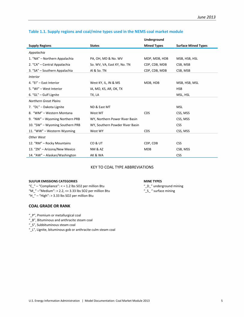
Coal supply regions Fourteen coal supply regions are represented in the CPS. The coal regions are listed in Table 1.1 and shown in Figure 1.1. The coal supply regions represented include States and regions in which prospective changes in coal use are likely to have the greatest market impacts.

The geographical split for the two Wyoming Powder River Basin (PRB) supply regions is primarily based on differences in the average heat content of the coal reserves in these regions. Production from mines in the Wyoming Northern PRB region have a heat content of approximately 16.8 million Btu per ton3 (8,400 Btu per pound), and production from mines in the Wyoming Southern PRB region have a slightly higher heat content of about 17.6 million Btu per ton (8,800 Btu per pound). In developing our base-year (2011) input data for AEO2013, the Wyoming Northern PRB supply region included production from the nine Wyoming PRB coal mines located north of the Black Thunder mine, and the Wyoming Southern PRB region included production from the three southernmost mines in Wyoming’s PRB (Arch Coal’s Black Thunder mine, Peabody’s North Antelope/Rochelle mine, and Cloud Peak Energy’s Antelope mine). In addition to heat content, the supply curves for the two Wyoming PRB supply regions have slightly different assignments for sulfur and mercury content (see Table 2.1).

Coal typology The model's coal typology includes four thermal and three sulfur grades of coal for surface and underground mining. The four thermal grades correspond generally to the three ranks of coal (bituminous, subbituminous, and lignite) and a premium grade bituminous coal used primarily for metallurgical purposes. The three sulfur grades represented are low, medium, and high. The three sulfur content categories are required to model the regulatory restrictions on SO2 emissions and to accurately estimate projected levels of SO2 emissions for the electric power sector. While each of the coal supply curves represented in the CMM are grouped into one of three sulfur grades, actual sulfur content assignments for each curve are based on regional-level data and, therefore, vary across the supply regions. For example, the average sulfur content of low-sulfur bituminous coal shipments from mines in Central Appalachia in recent years has been about 0.55 pounds per million Btu heat input, while the sulfur content of low-sulfur subbituminous coal shipped from mines in Wyoming’s Southern Powder River has averaged less than 0.35 pounds per million Btu heat input. In total, nine coal types (unique combinations of thermal grade and sulfur content) and two mine types (underground and surface) are represented in the CPS (Table 1.1).

For AEO2013, U.S. coal supply is represented through the use of 41 supply curves, reflecting the combination of supply regions, coal types, and mine types (Table 1.1). The required number of coal supply curves varies by region because not all coal types are represented in the coal reserve base for each of the 14 supply regions modeled in the CMM. For example, Northern Appalachia is represented with six supply curves, the most of any of the regions, while the Western Interior, Dakota Lignite, and

3Unless otherwise specified, tons refer to short tons (2,000 pounds) throughout this document.

June 2013


Alaska/Washington regions are each represented with a single supply curve. In some instances, the coal reserves base for a region may contain coal types that are not represented in the CMM, generally because the quantity of available reserves is felt to be of an insufficient quantity to model. An example is the small quantities of low-sulfur, bituminous coal reserves that are not modeled for the Northern Appalachian supply region.4

The primary data source for U.S. coal reserves is the demonstrated reserve base (DRB) of coal in the United States. Although the DRB was originally developed by the U.S. Bureau of Mines in 1971, EIA assumed responsibility for the DRB in 1977 and has since maintained and updated the information for this important database.5 Over time, EIA has performed two general types of updates: (1) annual downward adjustments to estimated coal reserves based on reported production from mines; and (2) regional updates to reserve estimates primarily based on new data from state geological surveys.

Model inputs and outputs Model input requirements are grouped into two categories, as follows:

• User-specified inputs • Inputs provided by other NEMS modules and submodules

User-specified inputs for the base year include capacity utilization at mines, productive capacity, minemouth coal prices, miner wages, labor productivity, cost of mining equipment, and the price of electricity. Other user-specified inputs required for the NEMS forecast years include annual growth rates for labor productivity and wages, and annual producer price indices for the cost of mining machinery and equipment, iron and steel, and explosives. Inputs obtained from other NEMS modules include coal production for year t-1, the minemouth coal price for years t and t-1, electricity prices, and the real interest rate (Figure 1.2). Appendix 1.C includes a complete list of input variables and specification levels.

The primary outputs of the model are annual coal supply curves (price/production schedules), provided for each supply region, mine type, and coal type.

4 U.S. Energy Information Administration, U.S. Coal Reserves: 1997 Update, DOE/EIA-0529(97) (Washington, DC, February 1999). 5 U.S. Energy Information Administration, Estimation of U.S. Coal Reserves by Coal Type: Heat and Sulfur Content, DOE/EIA-0529 (Washington, DC, October 1989), p. 5.

June 2013


Table 1.1. Supply regions and coal/mine types used in the NEMS coal market module

Supply Regions States

Underground

Mined Types Surface Mined Types

Appalachia

1. “NA” – Northern Appalachia

2. “CA” – Central Appalachia

3. “SA” – Southern Appalachia

PA, OH, MD & No. WV

So. WV, VA, East KY, No. TN

Al & So. TN

MDP, MDB, HDB

CDP, CDB, MDB

CDP, CDB, MDB

MSB, HSB, HSL

CSB, MSB

CSB, MSB

Interior

4. “EI” – East Interior

5. “WI” – West Interior

6. “GL” – Gulf Lignite

West KY, IL, IN & MS

IA, MO, KS, AR, OK, TX

TX, LA

MDB, HDB

MSB, HSB, MSL

HSB

MSL, HSL

Northern Great Plains

7. “DL” – Dakota Lignite

8. “WM” – Western Montana

9. “NW” – Wyoming Northern PRB

10. “SW” – Wyoming Southern PRB

11. “WW” – Westerm Wyoming

ND & East MT

West MT

WY, Northern Power River Basin

WY, Southern Powder River Basin

West WY

CDS

CDS

MSL

CSS, MSS

CSS, MSS

CSS

CSS, MSS

Other West

12. “RM” – Rocky Mountains

13. “ZN” – Arizona/New Mexico

14. “AW” – Alaskan/Washington

CO & UT

NM & AZ

AK & WA

CDP, CDB

MDB

CSS

CSB, MSS

CSS

KEY TO COAL TYPE ABBREVIATIONS

SULFUR EMISSIONS CATEGORIES MINE TYPES “C_” – “Compliance”: < = 1.2 lbs SO2 per million Btu “_D_” underground mining “M_” –“Medium”: > 2.2, <= 3.33 lbs SO2 per million Btu “_S_ “ surface mining “H_” – “High”: > 3.33 lbs SO2 per million Btu

COAL GRADE OR RANK

“_P”, Premium or metallurgical coal “_B”, Bituminous and anthracite steam coal “_S”, Subbituminous steam coal “_L”, Lignite, bituminous gob or anthracite culm steam coal

June 2013


Figure 1. 1. Coal supply regions

Source: U.S. Energy Information Administration, Office of Electricity, Coal, Nuclear and Renewables Analysis.

June 2013


Relationship to other components of NEMS The model generates regional mid-term (to 2040) coal supply curves. A distinct set of supply curves is determined for each forecast year. The supply curves are required input to the CDS submodule of the CMM, and the NEMS Electricity and Liquid Fuels Market Modules. The information flow between the model and other components of NEMS is shown in Figure 1.2. Information obtained from the CDS and other NEMS modules is as follows:

• Electricity prices by Census division are obtained from the Electricity Market Module (EMM) in year t

• National-level distillate fuel price is obtained from the Liquid Fuels Market Module (LFMM) in year t

• Real interest rate is obtained from the Macroeconomic Activity Module (MAM) in year t • Coal production by CPS supply curve in year t-1 • Minemouth coal prices by CPS supply curve in years t and t-1

Model rationale

Theoretical approach The purpose of the CPS is to construct a distinct set of coal supply curves for each forecast year in NEMS. The construction of these curves involves three main steps for any given forecast year. First, the CPS calibrates the regression model to base-year production and price levels by region, mine type, and coal type. Second, the CPS converts the regression equation into coal supply curves. Finally, the supply curves are converted to step-function form for input to the CMM’s Coal Distribution Submodule, which finds the least cost solution (minemouth price plus transportation cost) of satisfying the projected annual levels of domestic and international coal demand.

The CPS addresses the relationship between the minemouth price of coal and corresponding levels of capacity utilization at mines, productive capacity, labor productivity, wages, fuel costs, other mine operating costs, and a term representing the annual user cost of mining machinery and equipment. These relationships are estimated through the use of a regression model that makes use of annual historical regional level data. The regression equation, together with projected levels of productive capacity, labor productivity, miner wages, capital costs, fuel prices and other mine operating costs, produces minemouth price estimates for coal by region, mine type, and coal type for different levels of capacity utilization.

Underlying rationale This section presents the econometric model used to produce coal supply curves for the AEO2013 forecasts. The primary criteria guiding the development of the coal pricing model were that the model should conform to economic theory and that parameter estimates should be unbiased and statistically significant. Following economic theory, an increase in output or factor input prices should result in higher minemouth prices, and increases in coal mining productivity should result in lower minemouth prices. In addition, the model should account for a substantial portion of the variation in minemouth prices over the historical period of study.

June 2013


Figure 1.2.

Background discussion and theoretical foundation Between 1978 and 2004, the average mine price of coal in the United States, in constant 2005 dollars, fell from $54.11 per ton to $20.74 per ton, a decline of 62 percent (Figure 1.3). During the same period, total U.S. coal production increased by 66 percent, from 670 million tons to 1,112 million tons. The inverse relationship between the production of coal and its price over time is attributable to many factors, including gains in labor productivity and declines in factor input costs. Although minemouth prices and coal mining productivity remained relatively constant between 1999 and 2004, both have changed significantly during the past few years. Between 2004 and 2011, the average U.S. minemouth coal price, in inflation adjusted dollars, rose by 74 percent. During this period, coal mining productivity declined by 24 percent, falling from 6.80 tons per miner hour to 5.19 tons per miner hour.

Coal Production Submodule

Electricity Market Module

Coal Distribution Submodule Coal Production (Year t - 1)

Minemouth Price of Coal (Years t and t - 1)

Coal Supply Curves (Year t)

Electricity Prices (Year t)

Macroeconomic Activity Module

Real Interest Rate (Year t)

Liquid Fuels Market Module

Price of Distillate Fuel (Year t)

Coal Supply Curves (Year t through Year t+20)

Do While NEMS/Coal Iteration is Less Than Final

Iteration (Year t)

Coal Supply Curves (Year t)

Figure 1.2. Information flow between the CPS and other components of NEMS

June 2013


Figure 1. 3. U. S. coal production and prices, 1978-2011

Productivity has had a profound effect on competition in the U.S. coal industry. Between 1978 and 2004, labor productivity at U.S. mines rose from 1.77 tons per miner hour to 6.80 tons per miner hour, representing an increase of 5.3 percent per year. This growth contributed to a downward shift in costs over time, making additional quantities of coal available at lower prices. A graphical representation of labor productivity and the average price of coal at mines for the unique combinations of region, mine type, and year as represented in the AEO2013 coal pricing model indicates the strong negative historical correlation between prices and productivity (Figure 1.4).

0.0

0.2

0.4

0.6

0.8

1.0

1.2

1.4

1.6

1.8

2.0

1978 1982 1986 1990 1994 1998 2002 2006 2010

Index (1978=1.00)

Production (Tonnage Based Index)

Average Mine Price (Constant-Dollar Index)

June 2013


Figure 1.4. Minemouth coal prices and labor productivity for CMM regions and mine types, 1978-2011

A model of the coal market

The model of the U.S. coal market developed for the CPS recognizes that prices in a competitive market are a function of factors that affect either the supply or demand for coal.6 The general form of the model is that a competitive market converges toward equilibrium, where the quantity supplied equals the quantity demanded for region i and mining type j in year t:

Q i,j,tS = Q i,j,tD= Q i,j,t (1.1)

In this equality, Q i,j,t represents the long-run equilibrium quantity of supply and demand for coal in a competitive market.

The formal specification of the coal pricing model for AEO2013 is as follows.

For demand,

Q i,j,tD = f (P, ELECt-1, ELEC_SHAREt-1, INDUSTRYt-1, OTHPRODt-1, EXPORTSt-1, PGASi,t, (1.2)

WOPt, STOCKSt-1, DAYS_SUPt-1,BTU_TONi,j,t, SULFURi,j,t, ASHi,j,t) + ei,j,tD

For supply,

P = f ((Qi,j,tS /PRODCAPi,j,t), PRODCAPi,j,t, TPHi,j,t, WAGEt, PCAPt, PFUELi,t, OTH_OPERi,j,t) + ei,j,t

S (1.3)

6 K. Forbes and C. Minnucci, Science Applications International Corporation, “An Econometric Model of Coal Supply: Final Report” (unpublished report prepared for the U.S. Energy Information Administration, December 20, 1996).

0

10

20

30

40

50

60

70

80

90

100

0 10 20 30 40 50Short Tons per Miner Hour

2005 Dollars per Short Ton

June 2013


The term “QS/PRODCAP” is the average annual capacity utilization at coal mines. Throughout the remaining sections and appendices of Section 1, this term is referred to as “CAPUTIL.”

The demand-side variables are as follows:

QD is the quantity of coal demanded from region i, mine type j, in year t in million tons.

ELEC is U.S. coal-fired electricity generation in billion kilowatthours in year t-1.

ELEC_SHARE is the share of total U.S. electricity generation accounted for by generation at natural-gas-fired power plants in year t-1.

INDUSTRY is U.S. industrial coal consumption (steam and coking) in million short tons for each year t-1.

OTHPROD is the total U.S. coal production in million tons minus coal production for region i and mine type j for each year t-1.

EXPORTS is the level of U.S. coal exports in million tons in year t-1.

PGAS is the delivered price of natural gas to the electricity sector in constant 1992 dollars per thousand cubic feet for region i in year t.

WOP is the world oil price in constant 1992 dollars per barrel in year t.

STOCKS is the quantity of coal inventories held at plants in the electric power sector in million tons at the beginning of year t-1.

DAYS_SUP is the average days of supply of coal inventories held at electricity sector plants in year t-1.

BTU_TON is the average heat content of coal receipts at electric power sector plants in million Btu per ton for region i and mine type j, in year t.

SULFUR is the average sulfur content of coal receipts at electric power sector plants specified as pounds of sulfur per million Btu for region i and mine type j, in year t.

ASH is the average ash content of coal receipts at electric power sector plants specified as percent ash by weight for region i and mine type j, in year t.

eD is a random term representing unaccounted factors in the demand function for region i and mine type j, in year t.

The supply-side variables are as follows:

P is the average minemouth price of coal in constant 1992 dollars per ton for region i and mine type j, in year t.

QS is the quantity of coal supplied in million tons from region i, mine type j, in year t.

PRODCAP is the annual coal productive capacity in million tons for region i and mine type j, in year t.

June 2013


QS/PRODCAP (or CAPUTIL) is the average annual capacity utilization (in percent) at coal mines for region i and mine type j, in year t.

TPH is the average annual labor productivity of coal mines in tons per miner hour for region i and mine type j, in year t.

WAGE is the average annual coal industry wage in constant 1992 dollars for region i, in year t.

PCAP is the annualized user cost of mining equipment in constant 1992 dollars, for mine type j, in year t.

PFUEL is the weighted average of the price of electricity in the industrial sector and the price of No. 2 diesel fuel to end users (excluding taxes) in 1992 dollars per million Btu for region i, in year t.

OTH_OPER is a constant-dollar index representing a measure for mine operating costs other than wages and fuel specified by supply region i, mine type j, in year t. Examples of other operating costs include items such as replacement parts for equipment, roof bolts, and explosives.

eS is a random term representing unaccounted factors in the supply function for region i and mine type j, in year t.

In this model, the amount of coal demanded from region i and mine type j in year t is determined by the minemouth price of coal, electricity generation, industrial coal consumption, coal exports, the price of natural gas, the world oil price, the level of coal stocks, and the heat, sulfur and ash content of the coal. On the supply side of the market, the minemouth price is assumed to be determined by the capacity utilization at mines, productive capacity, the level of labor productivity, the average level of wages, the annualized cost of mining equipment, and the cost of fuel used by mines.

Estimation methodology

The supply function for coal cannot be evaluated in isolation when the relationship between quantity and price is being studied. The solution is to bring the demand function into the picture and estimate the demand and supply functions together. For the AEO2013 coal pricing model, the two-stage least squares (2SLS) methodology was selected for estimating the set of simultaneous equations representing the supply and demand for coal.

The rationale for using 2SLS rather than ordinary least squares (OLS) results from the structure of equations (1.2) and (1.3). In equation (1.3), the error term in the supply equation (eS) affects the minemouth price (P); however, in Equation (1.2), price influences the quantity demanded (QD). As a result, the quantity of coal supplied (QS) on the right-hand side of the supply equation is correlated with the error term in the same equation. This violates one of the fundamental assumptions underlying the use of OLS, namely, that the error term is independent from the regressors. As a result, the OLS estimator will not be consistent.

In addition, while WAGE, PCAP, PFUEL, OTH_OPER, and TPH are all hypothesized to affect the price of coal, they are also affected by the price of coal. For example, an increase in the price of coal resulting from increased demand for coal may affect the wages paid in the coal industry, the cost of mining

June 2013


equipment, and the price of fuels. Prices may also influence the level of productivity. If prices decrease (increase), marginal mines are abandoned (opened), increasing (lowering) labor productivity. This violates the assumption underlying the use of OLS, making it an inappropriate method by which to estimate the supply function.

An accepted solution to the problem of biased least squares estimators is the use of 2SLS, where the objective is to make the explanatory endogenous variable uncorrelated with the error term. 7 This is accomplished in two stages. In the first stage of the estimation, the endogenous explanatory variables are regressed on the exogenous and predetermined variables. This stage produces predicted values of the endogenous explanatory variables that are uncorrelated with the error term. The predicted values are employed in the second stage of the technique to estimate the relationship between the dependent endogenous variable and the independent variables. The result from the second-stage (structural) equation represents the model implemented in the CMM for AEO2013. The first stage (reduced form) equations are used only to obtain the predicted values for the endogenous explanatory variables included in the second stage, effectively purging the demand effects from the supply-side variables.

The structural equation for the coal pricing model was specified in log-linear form using the variables listed above. In this specification, the values for all variables (except for the constant terms) are transformed by taking their natural logarithm. All observations were pooled into a single regression equation. In addition to the overall constant term for the model, intercept dummy variables were included for all regions except Central Appalachia. Slope dummy variables were included for the productivity and productive capacity variables to allow the coefficients for those terms to vary across regions and mine types. The Durbin-Watson test for first-order positive autocorrelation indicated that the hypothesis of no autocorrelation should be rejected. As a consequence, a correction for serial correlation was incorporated. In addition, a formal test indicated that the null hypothesis of homoskedasticity (the assumption that the errors in the regression equation have a common variance) across regions should be rejected, and, as a result, a weighted regression technique to correct for heteroskedasticity in the error term was employed to obtain more efficient parameter estimates. The statistical results of the regression analysis and the equation used for predicting future levels of minemouth coal prices by region, mine type, and coal type are provided in Appendix 1.D.

In general, the results satisfy the performance criteria specified for the model. Indicative of the high R2 statistic, there is a close correspondence between the predicted and actual minemouth prices (a discussion of how the R2 statistic is calculated in the TSP statistical package is provided in Appendix 1.D). Moreover, all parameter estimates have their predicted signs and are generally statistically significant.

Average annual seam thickness by region and mine type also was tested as a supply-side variable. The model results, however, did not support the hypothesis that decreases (increases) in seam thickness have exerted upward (downward) pressure on prices.

7 G.S. Maddala, Introduction to Econometrics: Second Edition (New York, MacMillan Publishing Company, 1992), 355-403.

June 2013


Labor productivity

Historically, the U.S. coal mining industry has developed or adopted a number of technological changes in each stage of production and achieved economies of scale that have contributed to overall productivity improvements. Examples include mining equipment and materials handling in underground mines, surface mining equipment and methods, equipment monitoring and automation, and mine planning. In the future, the rate at which productivity will advance is dependent on the mix of relatively new technologies that are contributing to the gains, their individual significance in realizing productivity improvement, and their stage in the technology diffusion cycle.

In addition to gradual improvements in mining equipment and techniques, the U.S. coal industry has also experienced the introduction and penetration of fundamentally new mining systems over time. At underground mines, examples include the introduction and gradual diffusion of the continuous mining method that began in the 1940s, and, more recently, the introduction and penetration of longwall mining systems that began in this country in the 1960s. Continuous mining saw its share of total U.S. underground production increase from 2 percent in 1951 to 31 percent in 1961. By 1971, the share of continuous mining coal production was 55 percent, and, in 1990, continuous mining accounted for 64 percent of total underground production. 8 Similarly, longwall mines saw their share of total underground production increase from less than 1 percent in 1966, to 4 percent in 1976, and to approximately 16 to 20 percent by 1982.9 Recent data collected by EIA showed continuing penetration of the longwall mining technique in the U.S. coal industry for another two decades, with this mining technique’s share of underground production rising to 29 percent in 1990 and to a peak of 53 percent in 2002.10 In 2011, longwall mines accounted for 49 percent of the production from all U.S. underground coal mines. For the future, it is likely that additional penetration of the longwall mining technique will be limited by a number of factors, such as concerns about surface subsidence and reduced availability of new sites with appropriate geologic characteristics and reserve blocks. The fragmentation of reserves and relatively thin coal seams of Central Appalachia are key factors underlying the recent decline in longwall production in this major supply region, where its share of underground production has dropped from a peak of 23 percent in 2003 to 13 percent in 2011. For surface mines, the size and capacity of the various types of equipment used (including shovels, draglines, front-end loaders, and trucks) has gradually increased over time, leading to steady growth in the average productivity of these mines.

Whether technological change represents improvements to existing technologies or fundamental changes in technology systems, the change has a substantial impact on productivity and costs. With few

8 J. I. Rosenberg, et al., Manpower for the Coal Mining Industry: An Assessment of Adequacy through 2000, prepared for the U.S. Department of Energy (Washington, DC, March 1979). 9 Paul C. Merritt, "Longwalls Having Their Ups and Downs," Coal, MacLean Hunter (February 1992), pp. 26-27. 10 U.S. Energy Information Administration (EIA), Coal Data: A Reference, DOE/EIA-0064(90) (Washington, DC, November 1991), p. 10; and EIA, Form EIA-7A, “Coal Production Report.”

June 2013


exceptions, transition in the coal industry to new technology has been gradual, and the effect on productivity and cost also has been gradual.11 The gradual introduction of new technology development is expected to continue during the NEMS forecasting horizon. Potential technology improvements in underground mining during the next several years include larger motors and improved designs of longwall shearers and continuous miners, larger conveyor motors and belt sizes for coal haulage, overall improvements in the design of underground coal haulage systems, better diagnostic monitoring of production equipment for preventive maintenance via the use of sensors and computers, and more precise control of longwall shearers and shields through the use of computer-supported equipment.12 Potential improvements in surface mining technology include the increased utilization of on-board computers for equipment monitoring, the increased use of blast casting for overburden removal, and the continuation in the long-term trend toward higher capacity equipment (e.g., larger bucket sizes for draglines and loading shovels and larger trucks for overburden and coal haulage).

In the CMM, different rates of productivity improvement are input for each of the 41 coal supply curves used to represent U.S. coal supply. In addition to assumptions about incremental improvements in coal mining technologies over the forecast horizon, the productivity inputs for the CMM also take into consideration the adverse impact on productivity that results as U.S. coal producers gradually move into more difficult-to-mine coal reserves. A fairly clear-cut example of a region where mining conditions are becoming increasingly difficult is Wyoming’s Powder River Basin, where coal producers are faced with steadily increasing overburden thicknesses as their surface mining operations advance to the west. This situation has faced coal producers in this region ever since the start of major surface mining operations in this region in the early 1970s. For years, advancements in mine equipment, mining techniques, and economies of scale appeared to have been winning out over the increasing overburden thicknesses at mines, as evidenced by steady improvements in coal mining productivity. For example, data collected by EIA and the Mine Safety and Health Administration indicate that coal mining productivity at mines in Wyoming’s Powder River Basin rose from 12.18 tons per miner hour in 1978 to 46.77 tons per miner hour in 2001. Since then, however, productivity for this region has leveled off and declined, with the most recent data indicating productivity of 32.94 tons per miner hour in 2011. This seems to be an indication that the more difficult mining conditions in this region are outpacing the advancements in surface coal mining technologies.

11 Perhaps the most notable exception has been the dramatic, ongoing rise in longwall productivity, following rapidly on the heels of the introduction of a new generation of longwall equipment in the last decade. Between 1986 and 1990, longwall productivity nearly doubled, and although this increase should not be attributed solely to the improvements in longwall technology, the introduction and rapid penetration of the new longwall equipment was unquestionably a major contributing factor. 12 S. Fiscor, “U.S. Longwall Census,” Coal Age (February 2013) and prior issues; E.J. Flynn, “Impact of Technological Change and Productivity on the Coal Market,” Issues in Midterm Analysis and Forecasting 2000, U.S. Energy Information Administration, EIA/DOE-0607(2000) (Washington, DC, July 2002); S.C. Suboleski, et. al., Central Appalachia: Coal Mine Productivity and Expansion (EPRI Report Series on Low-Sulfur Coal Supplies) (Palo Alto, CA: Electric Power Research Institute (Publication Number IE-7117), September 1991).

June 2013


In the CMM, the cost effect of labor productivity change for each year is determined using the coal-pricing regression model which incorporates both regional and mine type coefficients. In each forecast year, the regression model determines the change in cost due to the changes in labor productivity and the costs of factor inputs. This calculation is based on exogenous productivity forecasts together with forecasts of the various factor input costs. The cost factor inputs to mining operations captured by the model include projected and estimated changes in real labor costs, real electricity and diesel fuel prices, other mine operating costs, and the annualized cost of capital over the forecast period.

Model structure This chapter discusses the modeling structure and approach used by the CPS to construct coal supply curves. The chapter provides a general description of the model, including a discussion of the key relationships and procedures used for constructing the supply curves. A detailed mathematical description of the CPS, showing the estimating equations and the sequence of computations, is provided in Appendix 1.B.

The model constructs a distinct set of supply curves for each forecast year in three separate steps, as follows (see Figure 1.5):

Step 1: Calibrate the regression model to base-year production and price levels by region, mine type and coal type

Step 2: Convert regression equation to continuous-function supply curves

Step 3: Construct step-function supply curves for input to the CDS

June 2013


Figure 1. 5. CPS flowchart

June 2013


Step 1: Model calibration To calibrate the model to the most recent historical data, a constant value is added to the regression equation for each CPS supply curve. Thus, when using the base-year values of the independent variables, the model solution will equal the base-year price as input by the user.

The calibration constants are automatically computed as part of a NEMS run. First, the coal-pricing equation is solved using the base-year values for the independent variables. Second, this estimated price is then subtracted from the actual base-year price input by the user. For calibration purposes the simplifying assumption is made that the lagged values of the independent variables (used in those terms of the equation needed to correct for autocorrelation) are the same as the base-year values. This assumption obviates the need to provide the model with two years of base data and is believed to yield a reasonable approximation of the “true” calibration constant.

Step 2: Convert regression equation to continuous supply curves A regression equation is used to estimate the relationship between minemouth prices and the projected or assumed values of production, productivity, wages, capital costs, and fuel prices. A distinct supply curve is developed for each combination of region, mine type, and coal type. For AEO2013, the CPS generated a set of 41 separate coal supply curves (see Table 1.1) for each year of the NEMS forecast period.

Following initial base-year calibration, the regression equations must be converted into supply curves in which price is represented as a function of production alone. This is accomplished by consolidating all of the non-capacity utilization terms in the regression equation into a single multiplier, computed using the forecast-year values of the independent variables. The value of the multiplier is computed by solving the regression equation with the capacity utilization term excluded and all other independent variables equal to their forecast-year values. A separate value of the multiplier is computed for each region, mine type, and coal type. Some of the required forecast-year values of the various independent variables are supplied endogenously by other NEMS modules, while others, including labor productivity, the average coal industry wage, and the PPI (producer price index) for mining machinery and equipment, steel and iron, and explosives are provided as user inputs. Two different PPI series are used to represent costs of mining equipment: one representing equipment used primarily at underground mines and a second representing equipment used primarily at surface mines.

It should be noted that the subroutine also contains code, currently “commented out,” which allows the user to compute the wage values based on inputs from the macroeconomic model; however, currently future wages are computed based on input data from the coal-user input data file referred to as the CLUSER file.

In the CPS, labor productivity is used as a way of capturing the effects of technological improvements on mining costs, in lieu of representing explicitly the cost impact of each potential, incremental technology improvement. In general, technological improvements affect labor productivity as follows: (1) technological improvements reduce the costs of capital; (2) the reduced capital costs lead to substitution of capital for labor; and (3) more capital per miner results in increased labor productivity. As determined by the econometric-based coal-pricing model developed for the CPS, increases in labor productivity translate into lower mining costs on a per-ton basis. Using this approach, exogenous

June 2013


estimates of labor productivity are provided to estimates of labor productivity are provided to the CPS for each year of the forecast period. Separate estimates are developed as inputs to the submodule for each region and mining method.

Step 3: Construct step-function supply curves The CDS is formulated as a linear program (LP) and cannot directly use the supply curves generated by the CPS regression model, whose functional form is logarithmic. Rather, the CDS requires step-function supply curves for input. Using an initial target quantity and percent variations from that quantity, an 11-step curve is constructed as a subset of the full CPS supply curve and is input to the CDS. For each supply curve and year, the CMM uses an iterative approach to find the target quantity that creates the optimal 11-step supply curve given the projected level of demand. The user can vary the length of the steps, and, subsequently, the vertical distances between the steps, by making adjustments to the percent variations from the target quantity via input parameters contained in the CLUSER input file. The selection of step-lengths for AEO2013 is based primarily on the premise that the model solution will lie close to the target quantity supplied by the CDS. As a result, the variation from the target quantity is fairly tight on the middle five to seven steps of the curve. The outer four steps are primarily there to assure that there is sufficient supply on the step-function curve to meet any substantial swings in coal demand that might result within a single iteration of NEMS.

The method by which these step-function curves are constructed is as follows. First, the CPS computes 11 quantities by multiplying the target quantity, obtained from the CDS, by the 11 user-specified scalars obtained from the CLUSER input file. The model then computes the prices corresponding to each of the 11 quantities, using the supply curve equations. Finally, prices for each step are adjusted to the year dollars required by the CDS using the GDP chain-type price index supplied by the NEMS Macroeconomic Activity Module. The resulting production and price values are used by the CDS to determine the least cost supplies of coal for meeting the projected levels of annual coal demand.

June 2013


\Appendix 1.A. Submodule Abstract Model name: Coal Production Submodule

Model abbreviation: CPS

Description: Produces supply-price relationships for 14 coal producing regions, nine coal types (unique combinations of thermal grade and sulfur content) and two mine types (underground and surface) addressing the relationship between the minemouth price of coal and corresponding levels of capacity utilization at coal mines, annual productive capacity, labor productivity, wages, fuel costs, other mine operating costs, and a term representing the annual user cost of mining machinery and equipment. The model serves as a major component in the National Energy Modeling System (NEMS). In the CPS, coal types are defined as unique combinations of thermal and sulfur content. This differs slightly from the NEMS Coal Distribution Submodule, where coal types are defined as unique combinations of thermal content, sulfur content, and mine type.

Purpose of the model: The purpose of the model is to produce annual domestic coal supply curves for the mid-term (to 2040) for the Coal Distribution Submodule of the Coal Market Module of NEMS.

Model update information: October 2012

Part of another model?: Yes, part of the:

• Coal Market Module • National Energy Modeling System

Model interface: The model interfaces with the following models:

• Coal Distribution Submodule • Electricity Market Module • Macroeconomic Activity Module • Liquid Fuels Market Module

Official model representative:

Office: Electricity, Coal, Nuclear and Renewables Analysis

Division: Coal and Electric Power

Model Contact: Mike Mellish

Telephone: (202) 586-2136

E-mail: [email protected]

June 2013


Documentation:

• U.S. Energy Information Administration, Coal Production Submodule Component Design Report (draft), May 1992, revised January 1993.

• U.S. Energy Information Administration, Coal Market Module of the National Energy Modeling System, Model Documentation 2013 DOE/EIA-M060(2013) (Washington, DC, June 2013).

Archive media and installation manual: NEMS13 - Annual Energy Outlook 2013

Energy system described by the model: Estimated coal supply at various FOB mine costs.

Coverage:

• Geographic: Supply curves for 14 geographic regions • Time Unit/Frequency: 2003 through 2040 • Product(s): nine coal types (unique combinations of thermal and sulfur content) and two

mine types (underground and surface) • Economic Sector(s): Coal producers and importers.

Modeling features:

• Model structure: The CPS employs a regression model to estimate price-supply relationships for underground and surface coal mines by region and coal type, using projected levels of capacity utilization at coal mines, annual productive capacity, productivity, miner wages, capital costs of mining equipment, fuel prices, and other variable mine supply costs.

• Modeling technique: Three main steps are involved in the construction of coal supply curves:

- Calibrate the regression model to base-year production and price levels by region, mine type (underground and surface), and coal type

- Convert the regression equation into supply curves

- Construct step-function supply curves for input to the CDS

• Model interfaces: Coal Distribution Submodule, Electricity Market Module, Macroeconomic

• Input data: Base-year values for U.S. coal production, capacity utilization, productive capacity, productivity, and prices. Base-year electricity prices and wages. Heat, sulfur, and mercury content averages, and carbon emission factors by supply curve. Projections of labor productivity, wages, the PPIs for mining machinery and equipment, iron and steel, and explosives.

June 2013


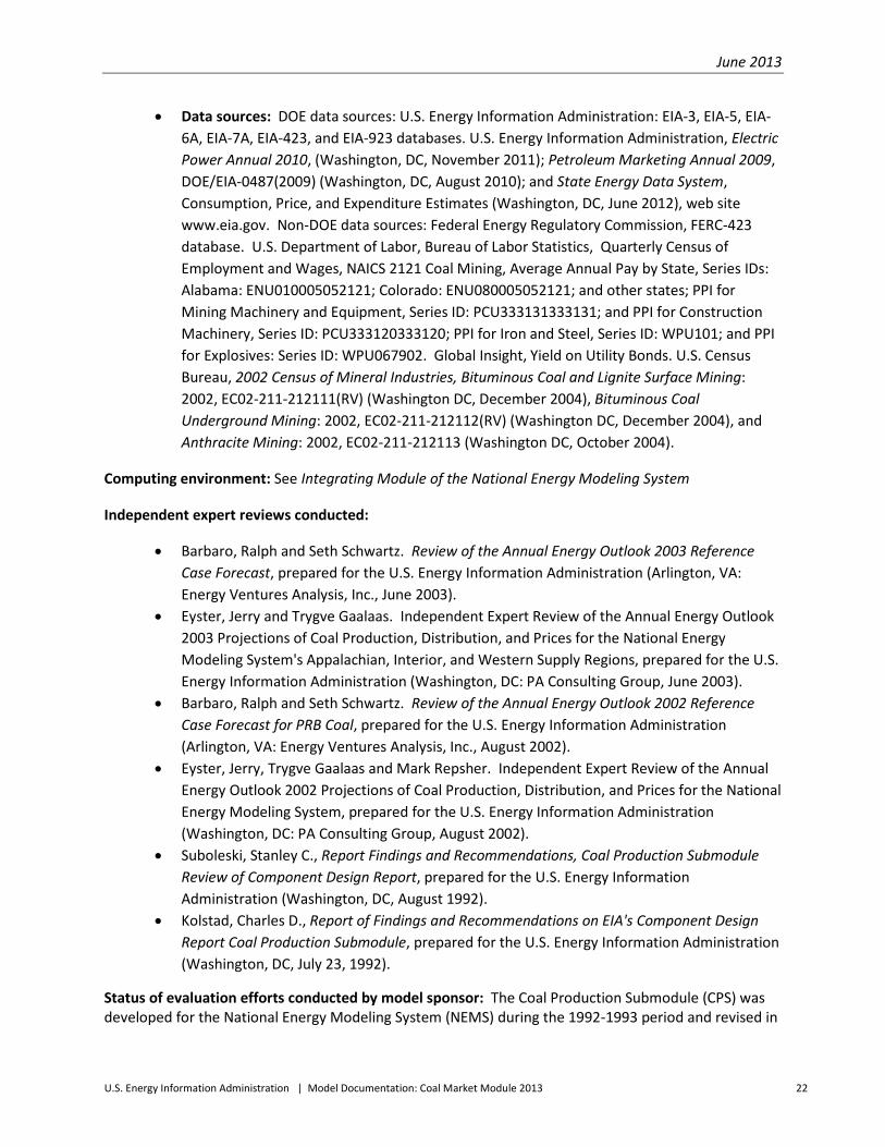
• Data sources: DOE data sources: U.S. Energy Information Administration: EIA-3, EIA-5, EIA-6A, EIA-7A, EIA-423, and EIA-923 databases. U.S. Energy Information Administration, Electric Power Annual 2010, (Washington, DC, November 2011); Petroleum Marketing Annual 2009, DOE/EIA-0487(2009) (Washington, DC, August 2010); and State Energy Data System, Consumption, Price, and Expenditure Estimates (Washington, DC, June 2012), web site www.eia.gov. Non-DOE data sources: Federal Energy Regulatory Commission, FERC-423 database. U.S. Department of Labor, Bureau of Labor Statistics, Quarterly Census of Employment and Wages, NAICS 2121 Coal Mining, Average Annual Pay by State, Series IDs: Alabama: ENU010005052121; Colorado: ENU080005052121; and other states; PPI for Mining Machinery and Equipment, Series ID: PCU333131333131; and PPI for Construction Machinery, Series ID: PCU333120333120; PPI for Iron and Steel, Series ID: WPU101; and PPI for Explosives: Series ID: WPU067902. Global Insight, Yield on Utility Bonds. U.S. Census Bureau, 2002 Census of Mineral Industries, Bituminous Coal and Lignite Surface Mining: 2002, EC02-211-212111(RV) (Washington DC, December 2004), Bituminous Coal Underground Mining: 2002, EC02-211-212112(RV) (Washington DC, December 2004), and Anthracite Mining: 2002, EC02-211-212113 (Washington DC, October 2004).

Computing environment: See Integrating Module of the National Energy Modeling System

Independent expert reviews conducted:

• Barbaro, Ralph and Seth Schwartz. Review of the Annual Energy Outlook 2003 Reference Case Forecast, prepared for the U.S. Energy Information Administration (Arlington, VA: Energy Ventures Analysis, Inc., June 2003).

• Eyster, Jerry and Trygve Gaalaas. Independent Expert Review of the Annual Energy Outlook 2003 Projections of Coal Production, Distribution, and Prices for the National Energy Modeling System's Appalachian, Interior, and Western Supply Regions, prepared for the U.S. Energy Information Administration (Washington, DC: PA Consulting Group, June 2003).

• Barbaro, Ralph and Seth Schwartz. Review of the Annual Energy Outlook 2002 Reference Case Forecast for PRB Coal, prepared for the U.S. Energy Information Administration (Arlington, VA: Energy Ventures Analysis, Inc., August 2002).

• Eyster, Jerry, Trygve Gaalaas and Mark Repsher. Independent Expert Review of the Annual Energy Outlook 2002 Projections of Coal Production, Distribution, and Prices for the National Energy Modeling System, prepared for the U.S. Energy Information Administration (Washington, DC: PA Consulting Group, August 2002).

• Suboleski, Stanley C., Report Findings and Recommendations, Coal Production Submodule Review of Component Design Report, prepared for the U.S. Energy Information Administration (Washington, DC, August 1992).

• Kolstad, Charles D., Report of Findings and Recommendations on EIA's Component Design Report Coal Production Submodule, prepared for the U.S. Energy Information Administration (Washington, DC, July 23, 1992).

Status of evaluation efforts conducted by model sponsor: The Coal Production Submodule (CPS) was developed for the National Energy Modeling System (NEMS) during the 1992-1993 period and revised in

June 2013


subsequent years. The version described in this abstract was used in support of the Annual Energy Outlook 2013.

Independent expert reviews of the Coal Market Module’s (CMM) Annual Energy Outlook 2002 and Annual Energy Outlook 2003 coal forecasts were conducted in August 2002 and June 2003, respectively, by Energy Ventures Analysis, Inc. (EVA) and the PA Consulting Group.

Last update: The CPS is updated annually for use in support of each year’s Annual Energy Outlook. The version described in this abstract was updated in October 2012.

June 2013


Appendix 1.B. Detailed Mathematical Description of the Model This appendix provides a detailed description of the model, including a specification of the model's equations and procedures for constructing the supply curves. The appendix describes the model's order of computations and main relationships. The model is described in the order in which distinct processing steps are executed in the program. These steps are as follows:

Step 1: Calibrate the regression model to base-year production and price levels by region, mine type, and coal type

Step 2: Convert the regression equation into supply curves


Indices

i = supply region

j = mining method (surface or underground)

k = coal type

t = year

by = base year (for AEO2013, the base year was 2011)

z = individual step on the step-function supply curves generated by the CPS for input to the Coal Distribution Submodule

Step 1: Initial calibration

Prior to the processing of inputs, the model calibrates the regression equation to current price levels. First, the equation for the CPS pricing model is used to calculate the minemouth price of coal for the base year as shown in equation 1.B-1. EXP represents the exponential function.

Pi,j,k,by = {EXP [(A + βj,1+ βi,2) * (1-rho)]}* [TPHi,j,t=1(TPHBM * (1-rho))] * (1.B-1)

CAPUTIL_HISTi,j,k[β

5 - (β

5 * CU_BY_SC)] * (1 - rho) *

[PROD_CAP_ADJi,j,k((β

3 + β

j,4+ PRODCAPADJ) * (1-rho))] *

[PRI_ADJi,j,k(-rho)] * [PRODCAPi,j,t=1

(PRODCAPBM * (1-rho))] *

PRODCAPi,j,k,by (β3 + β

j,4+ PCAPCADJ) * CAPUTILi,j,k,by (β5

* CU_BY_SC) *

TPHi,j,by ((β

6 + (TPHADJ)) + β

i,7 + β

j,8 + β

i,j,9) * WAGEi,by (β10

+ βj,11

) * PCAPj,by β12 * PFUELi,by β13 *

OTH_OPERi,j,by β14 * Pi,j,k,by rho * PRODCAPi,j,k,by (-rho * (β3 + β

j,4 + PRODCAPADJ) *

June 2013


CAPUTILi,j,k,by (-rho * β5 * CU_BY_SC) * TPHi,j,by (-rho * ((β6

+ (TPHADJ)) + βi,7

+ βj,8

+ βi,j,9

)) *

WAGEi,by (-rho * (β10 + β

j,11)) * PCAPj,by (-rho * β12

) * PFUELi,by (-rho * β13) *

OTH_OPERi,j,by (-rho * β14)

where CU_BY_SC = (CAPUTILi,j,k,by /CAPUTIL_HISTi,j,k) η

Variables

Pi,j,k,by - average annual minemouth price of coal for supply region i, mine type j, and coal type k, computed from the regression equation using base-year values of the independent variables

A - overall constant term for the model

TPHBM - Pricing model adjustment factor applied to overall constant term to account for user-specified revisions of the coefficient for the labor productivity regression variable

PROD_CAP_ADJi,j,k - factor used to adjust intercept for the model to account for the fact that the levels of productive capacity used to estimate the coal pricing equation were specified by mine type, while the model is implemented in NEMS by mine type and coal type

PRI_ADJi,j,k - factor used to adjust intercept for the model to account for the fact that the minemouth coal prices used to estimate the coal pricing equation were specified by mine type, while the model is implemented in NEMS by mine type and coal type

PRODCAPi,j,k,by - annual productive capacity of coal mines for supply region i, mine type j, and coal type k for the base year

PRODCAPBM - pricing model adjustment factor applied to overall constant term to account for user-specified revisions of the coefficient for the productive capacity regression variable

CAPUTILi,j,k,by - annual capacity utilization (the ratio of annual production to annual productive capacity) of coal mines for supply region i, mine type j, and coal type k for the base year (modeled as a percentage)

TPHi,j,by - coal mine labor productivity for supply region i and mine type j for the base year

TPHADJ - represents a potential user-specified change to the parameter estimate for the overall productivity term β6 (set to zero for AEO2013)

WAGEi,by - average annual wage for coal miners for supply region i for the base year

June 2013


PCAPj,by - index for the annual user cost of capital for mine type j, for the base year

PFUELi,by - weighted annual average of the electricity price and the diesel fuel price for supply region i for the base year

OTH_OPERi,j,by - constant-dollar index representing a measure for mine operating costs other than wages and fuel costs specified for supply region i and mine type j for the base year

PRODCAPADJ - represents a potential user-specified change to the parameter estimate for the productive capacity term β3 (set to 0.200 for AEO2013)

Pi,j,k,by - average minemouth price of coal for supply region i, mine type j, and coal type k for the base year

CAPUTIL_HISTi,j,k - representative coal-mine capacity utilization for the time period over which the coal pricing model is estimated for supply region i, mine type j, and coal type k

CU_BY_SC - scalar used to adjust regression coefficient for the capacity utilization term for levels of average coal-mine capacity utilization that lie outside the range of utilization rates contained in the coal pricing model’s historical database

η - exponent representing the theoretical functional form of the capacity utilization term for levels of capacity utilization that are outside the range of utilization rates contained in the coal pricing model database (for AEO2013, this term was set at 3.0)

Regression Coefficients

A overall constant for the model βj,1 for the intercept dummy variables for each mine type j βi,2 for the intercept dummy variables for each supply region i β3 for the productive capacity term βj,4 for the productive capacity term by mine type j β5 for the capacity utilization term β6 for the labor productivity term βi,7 for the labor productivity term by supply region i βj,8 for the labor productivity term by mine type j βi,j,9 for the labor productivity term by supply region i and mine type j β10 for the labor cost term βj,11 for the labor cost term by mine type j β12 for the user cost of capital term β13 for the fuel price term β14 for the other mine operating costs term rho for the first-order autocorrelation term

June 2013


For calibration purposes, base-year values of productive capacity, capacity utilization, productivity, labor costs, the fuel price, capital costs, and the average minemouth price are provided as inputs to the equation. Using these base-year values, the regression equation is solved for each CPS supply region, mining method, and coal type. Note that for calibration purposes the simplifying assumption is made that the lagged values of the independent variables (used in those terms of the equation needed to correct for autocorrelation) are the same as the base-year values. This assumption obviates the need to provide the model with two years of base data, and is believed to yield a reasonable approximation of the “true” calibration constant.

As shown in equation 1.B-2, the calibration constants are determined as the difference between the minemouth price of coal (Pi,j,k,by) calculated with the CPS pricing equation using base-year values for the independent variables and the corresponding base-year mine price of coal (BYPi,j,k), which is an input to the CLUSER file.

CAL_FACTORi,j,k = (BYPi,j,k - Pi,j,k,by) (1.B-2)

where

CAL_FACTORi,j,k - constant added to the regression equation for each supply region i, mine type j, and coal type k to calibrate the model to current price levels

BYPi,j,k - average base-year mine price for region i, mine type j, and coal type k

Pi,j,k,by - price computed from regression equation using base-year values of the independent variables, for region i, mine type j, and coal type k for the base year

The calibration constants thus calculated are used to make vertical adjustments to each CPS supply curve. Thus, when using the base-year values of the independent variables, the model solution will equal the base-year price as specified in the CLUSER file.

Step 2: Convert the regression equation into supply curves

Following initial base-year calibration, the regression equations must be converted into supply curves in which price is represented as a function of capacity utilization alone. This is accomplished by consolidating all of the non-capacity utilization terms in the regression equation into a single multiplier (Ki,j,k), computed using the forecast-year values of the independent variables as shown in equation 1.B-3.

Ki,j,k,t = {EXP [(A + βi,1+ βi,2) * (1-rhorho)]}* [TPHi,j,t=1(TPHBM * (1-rho))] * (1.B-3)

CAPUTIL_HISTi,j,k[β

5 - (β

5 * CU_FY_SC)] * ( - rho) *


3 + β

j,4+ PRODCAPADJ) * (1-rho))] *

[PRI_ADJi,j,k(-rho)] * [PRODCAPi,j,t=1

(PRODCAPBM * (1-rho))] *

PRODCAPi,j,k,t (β3 + β

j,4+ PRODCAPADJ) * TPHi,j,t

((β6

+ TPHADJ) + βi,7

+ βj,8

+ βi,j,9

) *

June 2013


WAGEi,t (β10 + β

j,11) * PCAPj,t β12 * PFUELi,t β13 *

OTH_OPERi,j,t β14 * Pi,j,k,t-1 rho * PRODCAPi,j,k,t-1 (-rho * (β3

+ βj,4

+ PRODCAPADJ)) *

CAPUTILi,j,k,t-1 (-rho * β5 * CU_FY_SC

) * TPHi,j,t-1 (-rho * ((β6

+ TPHADJ) + βi,7

+ βj,8

+ βi,j,9

)) *

WAGEi,t-1 (-rho * (β10

+ βj,11

)) * PCAPj,t-1 (-rho * β12) * PFUELi,t-1 (-rho * β13

) *

OTH_OPERi,j,t-1 (-rho * β14)

where

CU_FY_SC = (CAPUTILi,j,k,t-1 / CAPUTIL_HISTi,j,k) η

Variables

Ki,j,k,t - annual multiplier, specified by supply region i, mine type j, and coal type k, calculated by solving the CPS coal pricing equation for production equal to zero for year t equal to zero and all other independent variables set equal to their forecast-year values (for years t and t-1)

A - overall constant term for the model

TPHBM - benchmark factor used for calibrating the coal pricing equation to the actual value of the minemouth coal price in year one of the forecast period

PROD_CAP_ADJi,j,k - factor used to adjust intercept for the model to account for the fact that the levels of productive capacity used to estimate the coal pricing equation were specified by mine type, while the model is implemented in NEMS by mine type and coal type

PRI_ADJi,j,k - factor used to adjust intercept for the model to account for the fact that the minemouth coal prices used to estimate the coal pricing equation were specified by mine type, while the model is implemented in NEMS by mine type and coal type

PRODCAPi,j,k,t - annual productive capacity of coal mines for supply region i, mine type j, coal type k, and year t

PRODCAPADJ - represents a potential user-specified change to the parameter estimate for the productive capacity term β3 (set to 0.200 for AEO2013)

PRODCAPBM - pricing model adjustment factor applied to overall constant term to account for user-specified revisions of the coefficient for the productive capacity regression variable

TPHi,j,t - coal mine labor productivity for supply region i, mine type j, and year t

June 2013


TPHADJ - represents a potential user-specified change to the parameter estimate for the overall productivity term β6 (set to zero for AEO2013)

WAGEi,t - average annual wage for coal miners for supply region i, in year t

PCAPj,t - index for the annual user cost of capital for mine type j, in year t

PFUELi,t - weighted annual average of the electricity price and the diesel fuel price for supply region i and year t

OTH_OPERi,j,t - constant-dollar index representing a measure for mine operating costs other than wages and fuel costs specified for supply region i and mine type j, in year t

Pi,j,k,t-1 - average minemouth price of coal for supply region i, mine type j, coal type k, and year t-1, as determined in the final NEMS iteration for year t-1

PRODCAPi,j,k,t-1 - annual productive capacity of coal mines for supply region i, mine type j, coal type k, and year t-1

CAPUTILi,j,k,t-1 - average annual capacity utilization (the ratio of annual production to annual productive capacity) of coal mines for supply region i, mine type j, coal type k, and year t-1 (modeled as a percentage)

TPHi,j,t-1 - coal mine labor productivity for supply region i, mine type j, and year t-1

WAGEi,t-1 - average annual wage for coal miners for supply region i, in year t-1

PCAPj,t-1 - index for the annual user cost of capital for mine type j, in year t-1

PFUELi,t-1 - weighted annual average of the electricity price and the diesel fuel price for supply region i in year t-1

OTH_OPERi,j,t-1 - constant-dollar index representing a measure for mine operating costs other than wages and fuel costs specified for supply region i and mine type j, in year t-1


CU_FY_SC - scalar used to adjust regression coefficient for the capacity utilization term for levels of average coal-mine capacity utilization that lie outside the range of utilization rates contained in the coal pricing model’s historical database. This term differs from the CU_BY_SC term referenced in equation 1-B.1, in that it uses the projected levels of capacity utilization in place of the base-year capacity utilization data from the CLUSER input file.


June 2013


Regression Coefficients (values provided in Table 1.D-1)

A overall constant for the model βj,1 for the intercept dummy variables for each mine type j βi,2 for the intercept dummy variables for each supply region i β3 for the productive capacity term βj,4 for the productive capacity term by mine type j β5 for the capacity utilization term β6 for the labor productivity term βi,7 for the labor productivity term by supply region i βj,8 for the labor productivity term by mine type j βi,j,9 for the labor productivity term by supply region i and mine type j β10 for the labor cost term βj,11 for the labor cost term by mine type j β12 for the user cost of capital term β13 for the fuel price term β14 for the other mine operating costs term rho for the first-order autocorrelation term

A separate value of Ki,j,k,t is computed for each region i, mine type j, coal type k, and year t. Some of the required forecast-year values of the various independent variables are supplied endogenously by other NEMS modules (see Figure 2), while others, including labor productivity, the average coal industry wage, the PPI (producer price index) for mining machinery and equipment, the PPI for iron and steel, and the PPI for explosives, are provided as user inputs. In place of a user input for the PPI for iron and steel, the CLUSER input file also contains a switch which, if set equal to 1, provides for the use of the related PPI for metals and metal products data (series id: WPI10) supplied by the NEMS Macroeconomic Activity Module.

Incorporating the calibration constant and the production term, the CPS supply curves take on the following form (equation 1.B-4):

Pi,j,k,t = CAL_FACTORi,j,k+ [Ki,j,k,t * CAPUTILi,j,k,t β5] (1.B-4)

where

Pi,j,k,t - minemouth price of coal by supply region i, mine type j, and coal type k computed as a function of output (Qi,j,k,t)

CAL_FACTORi,j,k - constant added to the regression equation for each supply region i, mine type j, and coal type k to calibrate the model to current price levels

Ki,j,k,t - annual multiplier, specified by supply region i, mine type j, and coal type k, calculated by solving the CPS coal pricing equation for production equal to zero for year t equal to zero and all other independent variables set equal to their forecast-year values (for years t and t-1)

June 2013


CAPUTILi,j,k,t - average annual capacity utilization (the ratio of annual production to annual productive capacity) of coal mines for supply region i, mine type j, coal type k, and year t (modeled as a percentage)

β5 - regression coefficient for the capacity utilization term


The CDS is formulated as a linear program (LP) and cannot directly use the supply curves generated by the CPS regression model, whose functional form is logarithmic. Rather, the CDS requires step-function supply curves for input. Using an initial target quantity and percent variations from that quantity, an 11-step curve is constructed as a subset of the full CPS supply curve and is input to the CDS. For each supply curve and year, the CMM uses an iterative approach to find the target quantity that creates the optimal 11-step supply curve given the projected level of demand. The user can vary the length of the steps, and, subsequently, the vertical distances between the steps, by making adjustments to the percent variations from the target quantity via input parameters contained in the CLUSER input file.

The method by which these step-function curves are constructed is as follows. First, the CPS computes 11 quantities corresponding to fixed percentages of a target quantity obtained from the CDS. The model then computes the production corresponding to each of the 11 quantities, using the supply curve equations.

Equation 1.B-5 shows the CPS equation used for generating the prices for the step-function supply curves.

Pi,j,k,z,t = CAL_FACTORi,j,k + [Ki,j,k,t * CAPUTIL_HISTi,j,k ( β

5 - (β

5 * CU_STEP_SC) * (1.B-5)

(Qi,j,k,z,t / PRODCAPi,j,k,t )( β

5 * CU_STEP_SC)]

where

CU_STEP_SC = ((Qi,j,k,z,t / PRODCAPi,j,k,t ) / CAPUTIL_HISTi,j,k) η

Variables

Pi,j,k,z - price associated with step z for region i, mine type j, coal type k, and year t specified as a percent variation from the target price.

CAL_FACTORi,j,k - calibration constant for each supply curve

Qi,j,k,z - production associated with step z for region i, mine type j, coal type k, and year t (the target quantity is obtained from the CLUSER file for year one of the forecast period and from the CDS for all remaining years of the forecast period)

June 2013


β5 - regression coefficient for the capacity utilization term

Ki,j,k,t - multiplier for the non-production terms in the regression equation

PRODCAPi,j,k,t - annual productive capacity of coal mines for supply region i, mine type j, coal type k, and year t


CU_STEP_SC - scalar - used to adjust regression coefficient for the capacity utilization term for levels of average coal-mine capacity utilization that lie outside the range of utilization rates contained in the coal pricing model’s historical database


The scalar for the capacity utilization term reflects the basic premise that mining costs will increase substantially as the capacity utilization of coal mines approaches 100 percent. For most combinations of region and mine type, rates of coal-mine capacity utilization rarely approach 100 percent in the historical data series used to estimate the coal-pricing model. In general, the highest rates of capacity utilization are reported by captive lignite operations in Texas, Louisiana, and North Dakota. Between 1991 and 2011, the average annual capacity utilization for Texas lignite production ranged from a low of 90.3 percent in 1991 to a high of 98.5 percent in 2006. During this same period, the average annual capacity utilization for surface coal mines in Wyoming's Northern Powder River Basin ranged from a low of 65.1 percent in 1993 to a high of 93.2 percent in 2007.

Equation 1.B-6 shows the CPS equation used for generating the quantities for the step-function supply curves.

STEP_Qi,j,k,z,t = Qi,j,k,z,t - Qi,j,k,z-1,t (1.B-6)

where

STEP_Qi,j,k,z,t - quantity associated with step z for region i, mine type j, coal type k, and year t

Qi,j,k,z,t - production associated with step z for region i, mine type j, coal type k, and year t

Qi,j,k,z-1,t - production associated with step z-1 for region i, mine type j, coal type k, and year t

Finally, prices for each step are adjusted to the year dollars required by the CDS using the GDP chain-type price index supplied by the NEMS Macroeconomic Activity Module. The resulting production and price values are used by the CDS to determine the least cost supplies of coal for meeting the projected levels of annual coal demand. The specific outputs provided by the model are described in Appendix 1.C.

June 2013


Appendix 1.C. Inventory of Input Data, Parameter Estimates, and Model Outputs Model inputs

Model inputs are classified into two categories: user-specified inputs and inputs provided by other NEMS components.

CLUSER. User-specified inputs are listed in Table 1.C-1. The table identifies each input, the variable name, the units for the input, and the level of detail at which the input must be specified. Future levels of labor productivity are estimated by EIA. For AEO2013, productivity improvements are assumed to continue at a reduced rate over the forecast horizon. Rates of improvement are developed based on econometric estimates using historical data by region and by mine type (surface and underground). The average heat and sulfur content values are estimated from data obtained from the EIA-923 database for coal consumed at electric power plants and from the EIA-3 and EIA-5 databases for coal consumed at industrial facilities and coke plants, respectively.

The values for the input variables listed in Table 1.C-1 are contained in the file CLUSER – a single "flat" file – and are listed in the order of their appearance in this file. The CLUSER file contains six main groups of data: (1) forecast-year estimates for labor costs, coal-mine productivity, and the PPIs for mining machinery and equipment, iron and steel, and explosives; (2) base-year quantities for production, productive capacity, capacity utilization, prices, and coal quality (heat content, sulfur content, mercury content and carbon dioxide emission factors) by supply curve; (3) share of annual fuel costs at U.S. coal mines represented by electricity and diesel fuel; (4) coefficients for the CPS coal-pricing equation; (5) forecast-year production capacity limitations by supply curve (no near-term constraints on production capacity were input for AEO2013); and (6) capacity utilization trigger points by region and mine type used to determine when to add or retire coal-mining productive capacity. Each trigger point is assigned a unique multiplier used to adjust annual productive capacity either upward or downward.

The indices used in the tables are defined as follows:

i = supply region j = mine type (surface or underground) k = coal type t = year by = base year z = individual step on the step-function supply curves generated by the CPS for input to the Coal Distribution Submodule

June 2013


Table 1.C-1. User-specified inputs required by the CPS

CPS Variable

Name Description Specification Level Units

Variable Used in

this Report Source(s)

WAGE Real labor cost escalator National/year -- -- EIA projection

L_PROD Base-year productivity Supply region/

mine type/coal

type

Tons/miner hour LPi,j,by EIA-7A

FR_PROD Forecast-year productivity (as a

fraction of L_PROD)

Supply region/

mine type/coal

type/year

-- LPi,j,t EIA projection

ADJ_MMP_

MULT

Price adjustment variable

(multiplier)

Supply region/

mine type/coal

type/year

Scalar -- EIA estimate

ADJ_MMP_

ADD

Price adjustment variable

(additive)

Supply region/

mine type/coal

type/year

1987 Dollars/Ton -- EIA estimate

SBAS_REGION Alphabetic supply region code Supply region -- -- Model

definition

NBAS

Number of production records Supply region -- -- File

definition

CPROD_TYPE Alphabetic coal type code Supply region/

coal type

-- -- Model

definition

B_PROD Base-year (2011) production

(surface and deep)

Supply region/

mine type/coal

type

MMTons Pi,j,k,by EIA-7A

BTU Average heat content (surface

and deep)

Supply region/

mine type/coal

type

MMBtu/ton -- FERC-423

SULFUR Average sulfur content (surface

and deep)

Supply region/

mine type/coal

type

Lbs/MMBtu -- FERC-423

CAR Average carbon dioxide

emission factor (surface and

deep)

Supply region/

coal type

Lbs/MMBtu -- U.S. EPA

PRI Base-Year (2011) coal price

(surface and deep)

Supply region/

coal type

1987 Dollars/Ton -- EIA-7A

MERCURY Average mercury content

(surface and deep)

Supply region/

mine type/coal

type

Lbs/trillion Btu -- U.S. EPA

B_CAP_UTIL Base-Year (2011) capacity

utilization of coal mines

(surface and deep)

Supply region/

mine type

Fraction CAPUTILi,j,k,by EIA-7A

June 2013


Table 1.C-1. User-specified inputs required by the CPS (cont.)

CPS Variable

Name Description

Specification

Level Units

Variable Used in


B_PROD_CAP Base-Year (2011) productive

capacity (surface and deep)

Supply region/

mine type/coal

type

MMTons PRODCAPi,j,k,by EIA-7A

B_PROD_CAP_ADJ Factor used to adjust intercept

for the model to account for the

fact that the levels of productive

capacity used to estimate the

coal pricing equation were

specified by region and mine

type, while the model is

implemented in NEMS by

region, mine type and coal type

(unique combination of heat

and sulfur content)

Supply region/

mine type/coal

type

-- PROD_CAP_

ADJi,j,k,by

EIA-7A

PRI_ADJ Factor used to adjust intercept

for the model to account for the

fact that the minemouth coal

prices used to estimate the coal

pricing equation were specified

by region and mine type, while

the model is implemented in

NEMS by region, mine type and

coal type (unique combination

of heat and sulfur content)

Supply region/

mine type/coal

type

-- PRI_ADJi,j,k,by EIA-7A

UTIL_HIST Representative coal-mine

capacity utilization for the time

period over which the coal

pricing model is estimated

(surface and deep)

Supply region/

mine type/coal

type

Percent CAPUTIL_

HISTi,j,k

EIA specifica-

tion

ELEC_SHARE

Share of total fuel costs at mines

represented by electricity

Supply region/

mine type

Fraction -- U.S. Census

Bureau

DIST_SHARE

Share of total fuel costs at mines

represented by diesel fuel

Supply region/

mine type

Fraction -- U.S. Census

Bureau

OCONT Overall constant for CPS

regression model

National -- A Regression

analysis

LUTIL Pricing model coefficient

(capacity utilization term)

National -- β5 Regression

analysis

June 2013



CPS Variable


Variable Used in


LWAGE Pricing model coefficient (labor

cost term)


analysis

LPCAP Pricing model coefficient (cost of

capital term)


analysis

LPFUEL Pricing model coefficient (fuel

price term)


analysis

LPSTEEL Pricing model coefficient (other

operating costs term)


analysis

TPH Pricing model coefficient (overall

productivity term)


analysis

TPH_DEEP Pricing model coefficient (mine

type productivity term)

Mine type -- βj,8 Regression

analysis

LPRODCAP Pricing model coefficient (overall

productive capacity term)


analysis

RHO Pricing model coefficient (first-

order autocorrelation term)

National -- Rho Regression

analysis

PDUMM Pricing model adjustment factor

applied to overall constant term

to account for user-specified

revisions of the coefficient for

the labor productivity regression

variable

National -- TPHBM Regression

analysis

DEEPRODCAP Pricing model coefficient (mine

type productive capacity term)

Mine type -- βj,4 Regression

analysis

DEEPWAGE Pricing model coefficient (mine

type labor cost term)

Mine Type -- βj,11 Regression

analysis

LPRODCAP_ SDA Pricing model adjustment factor

applied to overall constant term

to account for user-specified

revisions of the coefficient for

the productive capacity

regression variable

National -- PRODCAPBM EIA specifica-

tion

DEEPCONT Pricing model coefficients

(intercept dummy variable for

mine type)

Mine Type -- βj,1 Regression

analysis

B_WAGE Base-year hourly wage National 1987 Dollars/Year WAGE Bureau of

Labor

Statistics

June 2013



CPS Variable


Variable Used in


F_INDEX Base-year electricity price

(industrial sector)

Supply region 1992 Dollars/

MMBtu

-- EIA

SDS Pricing model coefficients

(intercept dummy variables for

supply regions)

Supply region -- βi,2 Regression

analysis

SDD Pricing model coefficients (used

to adjust intercept terms for

underground mines in CPS

regions WM, WW and ZN)


analysis

SPROD Pricing model coefficients

(regional productivity terms)


analysis

DPROD Pricing model coefficients

(regional and mine type

productivity terms)

Supply region/

mine type

-- βi,j,9 Regression

analysis

P_EQUIP_ SURF PPI for construction machinery Year Constant-dollar

index (1992

dollars)

-- Bureau of

Labor

Statistics

P_EQUIP_

UNDG

PPI for mining machinery and

equipment

Year Constant-dollar

index (1992

dollars)

-- Bureau of

Labor

Statistics

PPI_METALS_

SWITCH

Switch to choose either the user-

specified PPI for iron and steel

(set switch to 0) or the NEMS-

generated PPI for metals and

metal products (set switch to 1)

-- -- -- --

P_STEEL PPI for iron and steel Year Constant-dollar

index (1992

dollars)

-- Bureau of

Labor

Statistics

P_EXPLO PPI for explosives Year Constant-dollar

index (1992

dollars)

-- Bureau of

Labor

Statistics

PCNT_REC Number of marginal

cost curves

National -- -- File

definition

PCNT_

REGION

Numerical supply

region identifier

Supply region -- -- Model

definition

PCNT_CTYPE Numerical coal

type identifier

Coal type -- -- Model

definition

June 2013



CPS Variable


Variable Used in


PCNT_PRICE Base-year minemouth coal price Supply region/

mine type/

coal type

1987 Dollars/ton -- EIA-7A

PCNT_PROD Initial target production used to

build step-

function curves with

11 steps

Supply region/

mine type/

coal type

MMTons -- EIA-7A

MCNT_REC Number of marginal

cost curves

National -- -- File

definition

MCNT_

REGION

Numerical supply

region identifier

Supply region -- -- Model

definition

MCNT_CTYPE Numerical coal

type identifier

Coal type -- -- Model

definition

MCNT_PRICE Initial target price

used to build

step-function curves

with 11 steps

Supply region/

mine type/

coal type

1987 Dollars/ton Pi,j,k,z=1,t EIA-7A

MCNT_PROD Base-year production

Supply region/

mine type/

coal type

MMTons -- EIA-7A

MCNT_STEP Variations from the target

price used to build

step-function curves

with 11 steps

National Fraction -- EIA

estimate

SCLIMIT_CNT Numerical supply curve code Supply curve -- -- Model

definition

SCLIMIT_REG Numerical supply region code Supply region -- -- Model

definition

SCLIMIT_

REGNAME

Alphabetic supply region code Supply region -- -- Model

definition

SCLIMIT_

CPSCT

Numerical coal type code Coal type -- -- Model

definition

SCLIMIT_

CDSCT

Alphabetic coal type code Coal type -- -- Model

definition

IYR Supply curve limit Supply curve MMTons -- EIA estimate

SCURVE_

LIMIT_MAX

Maximum supply curve limit National MMTons -- EIA specifica-

tion

June 2013



CPS Variable


Variable Used in


UTIL_EXP Real number used to revise the

coefficient for the coal pricing

model’s capacity utilization term

for levels of capacity utilization

that are outside the upper range

of utilization rates contained in

the coal pricing model database.

This factor (set to 3.0 for

AEO2013) is used for calculating

prices for each of the last six

steps of the eleven-step CPS

supply curves.

National -- η EIA specifica-

tion

UTIL_EXP_ BOT Real number used to revise the

coefficient for the coal pricing

model’s capacity utilization term

for levels of capacity utilization

that are outside the lower range

of utilization rates contained in

the coal pricing model database.

This factor (set to 1.0 for

AEO2013) is used for calculating

prices for each of the first five

steps of the eleven-step CPS

supply curves.

National -- η EIA specifica-

tion

UTIL_MAX_

SURF

Upper capacity utilization

amount used to trigger additions

to surface productive capacity

Supply region Fraction -- EIA specifica-

tion

UTIL_MAX_

UNDG

Upper capacity utilization


to underground productive

capacity


tion

UTIL_MID_

SURF

Mid-level capacity utilization


to surface productive capacity


tion

UTIL_MID_

UNDG

Mid-level capacity utilization


to underground productive

capacity


tion

June 2013



CPS Variable


Variable Used in


UTIL_MIN_

SURF

Lower capacity utilization

amount used to trigger

retirements of surface productive

capacity


tion

UTIL_MIN_

UNDG

Lower capacity utilization

amount used to trigger

retirements of underground

productive capacity


tion

UTIL_MAX_

SURF_ADJ

Factor used to increase surface

productive capacity when

capacity utilization

≥UTIL_MAX_SURF


tion

UTIL_MAX_

UNDG_ADJ

Factor used to increase

underground productive capacity

when capacity utilization

≥UTIL_MAX_UNDG


tion

UTIL_MID_

SURF_ADJ

Factor used to increase surface



≥UTIL_MAX_SURF but

UTIL_MID_SURF


tion

UTIL_MID_

UNDG_ADJ

Factor used to increase



≥UTIL_MAX_UNDG but

UTIL_MID_UNDG


tion

UTIL_MIN_

SURF_ADJ

Factor used to retire surface



≤UTIL_MIN_SURF


tion

UTIL_MIN_

UNDG_ADJ

Factor used to retire



≤UTIL_MIN_SURF


tion

MCNT_STEP Variable use to establish

production levels for each of the

11 steps represented on the CPS

step-function supply curves

National Fraction -- EIA specifica-

tion

June 2013


Inputs provided by other NEMS components. Table 1.C-2 identifies inputs obtained from other NEMS components and indicates the variable name, the units for the input, and the level of detail at which the input must be specified. Electricity prices are obtained from the Electricity Market Module, industrial distillate fuel prices are obtained from the Liquid Fuels Market Module, the real rate of interest on AA public utility bonds is received from the Macroeconomic Activity Module, and production and prices by CPS supply curve are obtained from the Coal Distribution Submodule (CDS).

Table 1.C-2. CPS inputs provided by other NEMS modules and submodules

CPS Variable Name Description

Specification

Level Units

Variable Used in

this Report

NEMS

Module/

Submodule

PELIN Average price of

electricity in the

industrial sector

Supply region/

year

1987 Dollars/

MMBtu

-- EMM

PDSIN Average price of

distillate in the

industrial sector

National/year 1987

Dollars/MMBtu

-- LFMM

MC_RLRMCORPPUAANS Real rate on AA-

rated public

utility bonds

National Percent -- MAM

LAG_PMPROD Total mine value

of coal produced

in year t-1

Supply region/

mine type/

coal type/year

1987 Dollars -- CDS

LAG_QPROD

Coal production

in year t-1

Supply region/

mine type/

coal type/year

Million tons -- CDS

MCNT_PROD

Target quantities

for years t > 1,

used to build

step-function

curves with 11

steps

Supply region/

mine type/

coal type/year

Million tons --

CDS

Model outputs

The primary outputs from the model are step-function supply curves provided to the CDS. In addition to the price and quantity values associated with the steps on each of the supply curves, the CPS provides the CDS with coal quality data that include estimates for heat, sulfur and mercury content, and for carbon dioxide emission factors (Table 1.C-3).

June 2013


Table 1.C-3. CPS model outputs

CPS Variable Name Description Units

Variable Used in this

Report

MCNT_P Minemouth coal price associated

with each CPS supply curve step

provided to the CDS

1987 dollars/ton Pi,j,k,z,t

MCNT_Q Length of each CPS supply curve step

provided to the CDS

Million tons Qi,j,k,z,t

MCNT_BTU Average Btu content for each CPS

supply curve step provided to the

CDS

MMBtu/ton --

MCNT_SULF Average sulfur content for each CPS

supply curve step provided to the

CDS

lbs/MMBtu --

MCNT_MERC Average mercury content for each

CPS supply curve step provided to

the CDS

lbs/Trillion Btu --

MCNT_CAR Average carbon dioxide emission

factor for each CPS supply curve step

provided to the CDS

lbs/MMBtu --

Endogenous variables

Variables endogenous to the model are included in Table 1.C-4. Table 1.C-4 includes the variable name used in the report, the corresponding variable name used in the CPS model, a description of the variable, and the variable's units.

June 2013


Table 1.C-4. Key endogenous variables

CPS Variable Name Description Units

Variable Used in this

Report

L_PROD Labor productivity for NEMS forecast

year t

Tons/miner hour TPHi,j,t

E_FUEL Hybrid fuel price (average of

industrial electricity and distillate

prices) for NEMS forecast year t

1992 dollars/

MMBtu

PFUELi,j,t

D_FUEL Diesel fuel prices for NEMS forecast

year t

1992 dollars/MMBtu --

R_WAGE Average coal industry wage for

NEMS forecast year t

1992 dollars/

year

WAGEi,t

PK User-cost of mining equipment for

NEMS forecast years

Constant-dollar index

(1992 dollars)

PCAPt

P_OPER_OTH Cost index representing operating

costs other than wages and fuel for

NEMS forecast year t

Constant-dollar index

(1992 dollars)

--

YINT CPS calibration constant -- Ci,j,k

FP Multiplier for non-production terms

in the CPS coal pricing equation

-- Ki,j,k,t

QTARG Target quantities for years t > 1,

used to build step-function curves

with 11 steps

Million tons

Qi,j,k,t

SC_PRICE Prices for each of the steps on the

11-step supply curves input to the

CDS

1992 dollars/ton Pi,j,k,z,t

SC_QUAN Quantities for each of the steps on

the 11-step supply curves input to

the CDS

Million tons Qi,j,k,z,t

LAG_PRI Minemouth price of coal by supply

curve in year t-1

1992 dollars/ton MMPi,j,k,t-1

LAG_PROD Coal production by supply curve in

year t-1

Million tons Qi,j,k,t-1

PROD_CAP Coal productive capacity by supply

curve in year t

Million tons PRODCAPi,j,k,t

June 2013


Appendix 1.D. Data Quality and Estimation Development of the CPS Regression Model

The two-stage least squares regression technique was used to estimate the relationship between the minemouth price of coal and the corresponding levels of capacity utilization at mines, productive capacity, labor productivity, wages, fuel costs, other mine operating costs, and a term representing the annual user cost of mining machinery and equipment. In the first stage of the estimation, the endogenous explanatory variables are regressed on the exogenous and predetermined variables. The product of this estimation is predicted values of the endogenous explanatory variables that are uncorrelated with the error term. In turn, these predicted values are employed in the second stage of the technique to estimate the relationship between the dependent endogenous variable and the independent variable(s).

The result from the second stage (structural) equation represents the model implemented in the CMM for AEO2013. The first stage (reduced form) equations are used only to obtain the predicted values for the endogenous explanatory variables included in the second stage, removing the effects on minemouth prices caused by shifts in the demand function.

The structural equation for the coal pricing model was specified in log linear (constant elasticity) form. In this specification, the values for all variables (except the constant term) are transformed by taking their natural logarithm. The CPS regression model was developed using a combination of cross-sectional and time series data. The model includes annual-level data for thirteen CPS supply regions 13 and two mine types (surface and underground) for the years 1978 through 2009, excluding the years 1986-1990.14 In all, 459 observations are included (18 observations per year (12 surface and five underground) for each of the 27 years represented in the historical data series).

13 Data for coal mines in the WI (IA,MO,KS,AR,OK,TX(Bit)) and AW (Alaska and Washington) supply regions were not included in the regression model. The average mine price of coal for most of the states in these two regions are withheld from EIA publications to avoid disclosure of individual company data. 14 The reason that data for the years 1986 through 1990 were excluded from the regression model was primarily due to lack of good quality data for U.S. coal mining productive capacity for the years 1987 through 1990. For these years, estimates of daily (1987-1989) and annual (1990) productive capacity were collected, but, because the data were not to be published, they did not go through a complete data verification process. Another complicating factor related to the coal mining productive capacity data is that for the years 1978 through 1989 EIA requested that respondents report estimated daily productive capacity on the EIA-7A “Coal Production Report” survey, while for the years 1990 and later survey respondents are asked to report estimated annual productive capacity. Because these are two very different measures of productive capacity, a methodology was developed to convert the earlier daily productive capacity data collected by EIA to annual productive capacity, thus enabling the use of additional years of data for estimating the regression model. Estimates of annual productive capacity by mine for the years 1978 through 1986 were developed using reported daily productive capacity data by mine, reported number of days worked by mine, and region/mine type estimates for maximum average number of days worked. The maximum average number of days worked represents the highest reported average number of days worked per year by region and mine type during the years 1978 through 1989. Annual productive capacity for mines that reported working less days than the maximum average number of days worked for their region and mine type were calculated by multiplying their reported daily productive capacity by the maximum average number of days worked. Alternatively, if a mine reported working more days than the maximum average number of days worked for their region/mine type, annual productive capacity was calculated by simply multiplying their reported daily productive capacity by their reported number of days worked.

June 2013


All data were pooled into a single regression equation. In addition to the overall constant term for the model, intercept dummy variables were included for most of the supply regions. Dummy variables were used for the productivity and productive capacity variables to allow slope coefficients to vary across regions and mine types. The Durbin-Watson test for first-order positive autocorrelation indicated that the hypothesis of no autocorrelation should be rejected. As a consequence, a correction for serial correlation was incorporated. In addition, a formal test indicated that the hypothesis of homoskedasticity (the assumption that the errors in the regression equation have a common variance) should be rejected, and, as a result, a weighted regression technique was employed to obtain more efficient parameter estimates.

The two-stage least squares (2SLS) regression equation for the CPS was estimated using the LSQ (general nonlinear least squares multiequation estimator) procedure in TSP 4.5 with the INST option. For a description of the LSQ procedure see the Reference Manual for TSP Version 4.5. The form of the CPS regression equation and the associated regression statistics are presented below and in Table 1.D-1, respectively. The sources for the various historical data series used in the regression model are shown in Tables 1.D-2 and 1.D-3.

Indicative of the high R2 statistic (see Table 1.D-1), there is a close correspondence between the predicted and actual minemouth prices. The calculation for the adjusted R2 statistic provided in Table 1.D-1 is documented in the User’s Guide for TSP Version 4.5. As indicated in this report, all of the statistics related to the residuals using the 2SLS regression technique are calculated in TSP with the same formulas used for ordinary least squares (OLS). A summary of the calculations used for generating the R2 and adjusted R2 statistics in TSP is provided below.

Computation of R2 with a constant term:

[ ]R e y yt t2 21 2= − −∑ ∑/ ( ) (1.D-1)

where

e y yt t t= −

and

y X bt t= Or

[ ]R SSR SST2 1= − /

where

SSR et= ∑ 2

SST y yt= −∑ ( )2

June 2013


The adjusted R2 or R 2 with a constant term is calculated as follows:

R SSR T K SST T2 1 1= − − −[ / ( )] / [ / ( )] (1.D-2)

In the above equations,

et residuals

yt observed values of the independent variable

y mean of the observed values of yt

yt predicted values of the independent variable

Xt vector of independent variables

b estimated regression coefficients

SSR sum of squared residuals

SST total sum of squares

T number of observations in the sample

K number of independent variables

Based on the regression results shown in Table 1.D-1, the equation used for predicting future levels of minemouth coal prices by region, mine type and coal type for AEO2013 is:

Pi,j,k,t = CAL_FACTORi,j,k,t + [Ci,j,k,t * PRODCAPi,j,k,t (β3 + β

j,4+ PRODCAPADJ) * (1.D-3)

CAPUTILi,j,k,t β5 * TPHi,j,t ((β

6 + TPHADJ) + β

i,7 + β

j,8 + β

i,j,9) * WAGEi,t (β10

+ βj,11

) * PCAPj,t β12 *

PFUELi,t β13 * OTH_OPERi,j,t β14 * Pi,j,k,t-1 rho * PRODCAPi,j,k,t-1 (-rho * (β3 + β

j,4+ PRODCAPADJ)) *

CAPUTILi,j,k,t-1 (-rho * β5 * CU_FY_SC

) * TPHi,j,t-1 (-rho * ((β6

+ TPHADJ) + βi,7

+ βj,8

+ βi,j,9

)) *

WAGEi,t-1 (-rho * (β10 + β

j,11)) * PCAPj,t-1 (-rho * β12

) * PFUELi,t-1 (-rho * β13) *

OTH_OPERi,j,t-1 (-rho * β14)]

First Term in Equation 1.D-3 (CAL_FACTORi,j,k,t)

CAL_FACTORi,j,k,t is a constant added to the regression equation for each supply region i, mine type j, and coal type k in each year t to calibrate the model to current price levels. For AEO2013, prices were calibrated to the average annual minemouth coal prices for 2011.

June 2013


Second Term in Equation 1.D-3 (Ci,j,k,t)

Ci,j,k,t = e(A + β1

+ βi,2

) * (1-rho) * TPHi,j,t=1 (TPHBM * (1-rho)) * CAPUTIL_HISTi,j,k

[β5

- (β5

* CU_FY_SC)] * ( - rho) * (1.D-4)


3 + β

j,4+ PRODCAPADJ) * (1-rho))] * [PRI_ADJi,j,k

(-rho)] *

[PRODCAPi,j,t=1 (PRODCAPBM * (1-rho))]

The first term in equation 1.D-4 (e(A + β1

+ βi,2

) * (1-rho)) is the intercept for the model, where "A" is an overall constant for the model, "β1" represents a mine specific constant for the model, and the term "βi,2" represents the regional specific constants for the model.

The second term in equation 1.D-4 (TPHi,j,t=1 (PCADJ * (1- rho))) represents an adjustment to the intercept term

for the coal-pricing equation to account for user-specified changes to the estimated coefficient for the overall productivity term β5. For AEO2013, PCADJ was set equal to zero reflecting the assumption that the estimated relationship between coal mining productivity and minemouth coal prices estimated for the historical period will continue to hold over the AEO2013 forecast horizon.

The third term in equation 1.D-4 (CAPUTIL_HISTi,j,k[β

5 - (β5 * CU_FY_SC)] * (- rho) ) represents a required adjustment to the intercept term for the coal-pricing equation to account for changes in the parameter estimate (β5) for the capacity utilization term. In the AEO2013 forecast scenarios, the coefficient for the capacity utilization term is revised endogenously within the Coal Market Module on the basis of how much the projected levels of capacity utilization vary from the representative historical levels of capacity utilization. This feature was added to the CPS to reflect the premise that coal mining costs will increase substantially as the average capacity utilization of coal mines approaches 100 percent. The term CU_FY_SC is equal to (CAPUTILi,j,k,t-1 / CAPUTIL_HISTi,j,k) η. In this equation, CAPUTILi,j,k,t-1 is the projected level of capacity utilization for a specific supply curve in year t-1, CAPUTIL_HISTi,j,k is the representative historical rate of capacity utilization for this same CPS supply curve, and the term η is a user-specified term. For AEO2013, the user-specified term η was set equal to 3.0.

The fourth term in equation 1.D-4 (PROD_CAP_ADJi,j,k((β

3 + β

j,4+ PRODCAPADJ) * (1-rho))) is used to adjust intercept

for the model to account for the fact that the levels of productive capacity used to estimate the coal pricing equation were specified by region and mine type, while the model is implemented in NEMS by region, mine type and coal type (unique combination of heat and sulfur content). PROD_CAP_ADJ is a user-specified input calculated by dividing base-year (2011) productive capacity for supply region i and mine type j by the estimated base-year (2011) productive capacity for supply region i, mine type j, and coal type k. The latter of these two productive capacity numbers represents data for a specific CPS supply curve, thus the additional coal type dimension for this term.

The fifth term in equation 1.D-4 (PRI_ADJi,j,k(-rho)) is used to adjust the intercept for the model to account

for the fact that the minemouth coal prices used to estimate the coal pricing equation were specified by region and mine type, while the model is implemented in NEMS by region, mine type and coal type (unique combination of heat and sulfur content). PRI_ADJ is a user-specified input calculated by dividing the average base-year (2011) minemouth coal price for supply region i and mine type j by the estimated average base-year (2011) minemouth coal price for supply region i, mine type j, and coal type k. The

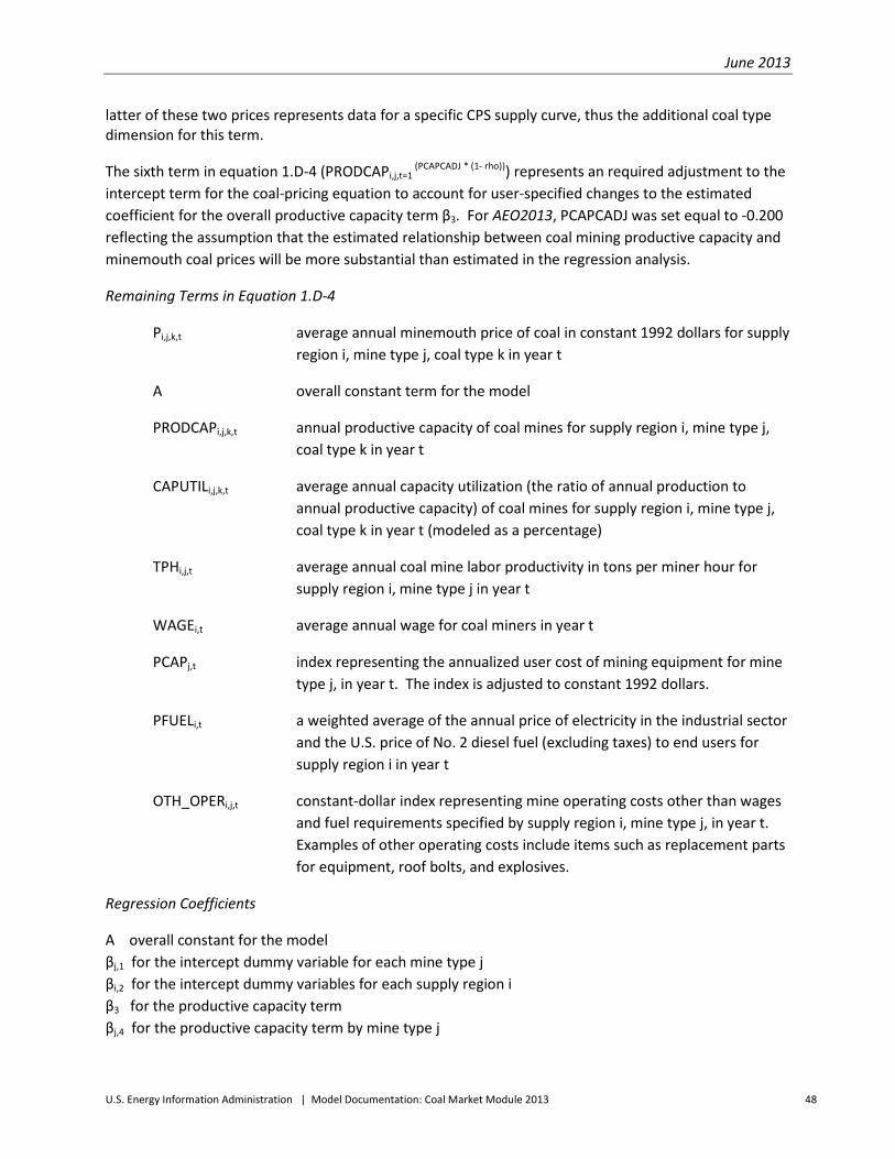
June 2013


latter of these two prices represents data for a specific CPS supply curve, thus the additional coal type dimension for this term.

The sixth term in equation 1.D-4 (PRODCAPi,j,t=1 (PCAPCADJ * (1- rho))) represents an required adjustment to the

intercept term for the coal-pricing equation to account for user-specified changes to the estimated coefficient for the overall productive capacity term β3. For AEO2013, PCAPCADJ was set equal to -0.200 reflecting the assumption that the estimated relationship between coal mining productive capacity and minemouth coal prices will be more substantial than estimated in the regression analysis.

Remaining Terms in Equation 1.D-4

Pi,j,k,t average annual minemouth price of coal in constant 1992 dollars for supply region i, mine type j, coal type k in year t

A overall constant term for the model

PRODCAPi,j,k,t annual productive capacity of coal mines for supply region i, mine type j, coal type k in year t

CAPUTILi,j,k,t average annual capacity utilization (the ratio of annual production to annual productive capacity) of coal mines for supply region i, mine type j, coal type k in year t (modeled as a percentage)

TPHi,j,t average annual coal mine labor productivity in tons per miner hour for supply region i, mine type j in year t

WAGEi,t average annual wage for coal miners in year t

PCAPj,t index representing the annualized user cost of mining equipment for mine type j, in year t. The index is adjusted to constant 1992 dollars.

PFUELi,t a weighted average of the annual price of electricity in the industrial sector and the U.S. price of No. 2 diesel fuel (excluding taxes) to end users for supply region i in year t

OTH_OPERi,j,t constant-dollar index representing mine operating costs other than wages and fuel requirements specified by supply region i, mine type j, in year t. Examples of other operating costs include items such as replacement parts for equipment, roof bolts, and explosives.

Regression Coefficients

A overall constant for the model βj,1 for the intercept dummy variable for each mine type j βi,2 for the intercept dummy variables for each supply region i β3 for the productive capacity term βj,4 for the productive capacity term by mine type j

June 2013


β5 for the capacity utilization term β6 for the labor productivity term βi,7 for the labor productivity term by supply region i βj,8 for the labor productivity term by mine type j βi,j,9 for the labor productivity term by supply region i and mine type j β10 for the labor cost term βj,11 for the labor cost term by mine type j β12 for the user cost of capital term β13 for the fuel price term β14 for the other mine operating costs term rho for the first-order autocorrelation term

Table 1.D-1. Regression statistics for the coal pricing model

Regression

Coefficient Variable

Parameter

Estimate

Standard

Error t- Statistic

A Overall Constant -3.479 1.329 -2.619*

βj=1,2 DUM_MINE_TYPE (Underground) -0.172 0.031 -5.552*

βi=3,2 DUM_REG3 (Southern Appalachia (SA)) 0.605 0.065 9.266*

βi=6,2 DUM_REG 6 (Gulf Lignite (GL)) -1.002 0.239 -4.191*

βi=7,2 DUM_REG 7 (Dakota Lignite (DL)) 0.480 0.235 2.046**

βi=8,2 DUM_REG 8 (Western Montana (WM)) 2.010 0.699 2.874*

βi=9,2 DUM_REG 9 (Wyoming, Northern PRB (NW)) 2.218 0.428 5.185*

βi=10,2 DUM_REG 10 (Wyoming, Southern PRB (SW)) 1.907 0.318 5.996*

βi=11,2 DUM_REG 11 (Western Wyoming (WW)) 0.884 0.257 3.436*

βi=12,2 DUM_REG 12 (Rocky Mountain (RM)) 0.360 0.061 5.920*

βi=13,2 DUM_REG 13 (Arizona/New Mexico (ZN)) 0.296 0.048 6.201*

β3 ln PRODCAP 0.205 0.025a 8.051*

β5 ln CAPUTIL 0.175 0.074 2.375**

β6 ln TPH -0.575 0.048 -11.994*

βi=6,7 GL*ln TPH 0.323 0.114 2.824*

βi=7,7 DL*ln TPH -0.272 0.084 -3.231*

βi=8,7 WM*ln TPH -0.670 0.236 -2.840*

βi=9,7 NW*ln TPH -0.743 0.126 -5.918*

βi=10,7 SW*ln TPH -0.613 0.097 -6.320*

βi=11,7 WW*ln TPH -0.314 0.133 -2.369**

βi=1,j=1,9 NA * DUM_ MINE_TYPE (Underground) * ln TPH 0.048 0.028 1.741***

βi=3,j=1,9 SA * DUM_ MINE_TYPE (Underground) * ln TPH -0.193 0.091 -2.132**

βi=12,j=1,9 RM * DUM_ MINE_TYPE (Underground) * ln TPH 0.238 0.043 5.600*

β10 ln WAGE 0.299 0.124 2.408**

β12 ln PCAP 0.134 0.033 4.089*

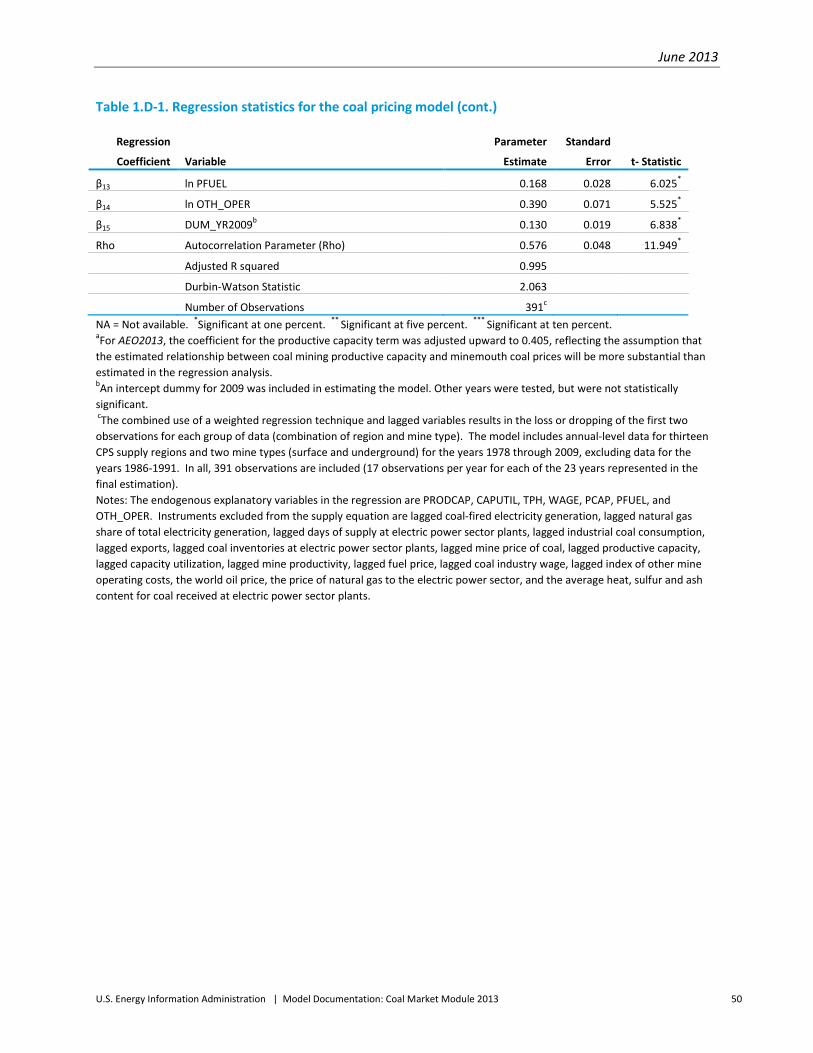
June 2013


Table 1.D-1. Regression statistics for the coal pricing model (cont.)

Regression

Coefficient Variable

Parameter

Estimate

Standard

Error t- Statistic

β13 ln PFUEL 0.168 0.028 6.025*

β14 ln OTH_OPER 0.390 0.071 5.525*

β15 DUM_YR2009b 0.130 0.019 6.838*

Rho Autocorrelation Parameter (Rho) 0.576 0.048 11.949*

Adjusted R squared 0.995

Durbin-Watson Statistic 2.063

Number of Observations 391c NA = Not available. *Significant at one percent. ** Significant at five percent. *** Significant at ten percent. aFor AEO2013, the coefficient for the productive capacity term was adjusted upward to 0.405, reflecting the assumption that the estimated relationship between coal mining productive capacity and minemouth coal prices will be more substantial than estimated in the regression analysis. bAn intercept dummy for 2009 was included in estimating the model. Other years were tested, but were not statistically significant. cThe combined use of a weighted regression technique and lagged variables results in the loss or dropping of the first two observations for each group of data (combination of region and mine type). The model includes annual-level data for thirteen CPS supply regions and two mine types (surface and underground) for the years 1978 through 2009, excluding data for the years 1986-1991. In all, 391 observations are included (17 observations per year for each of the 23 years represented in the final estimation). Notes: The endogenous explanatory variables in the regression are PRODCAP, CAPUTIL, TPH, WAGE, PCAP, PFUEL, and OTH_OPER. Instruments excluded from the supply equation are lagged coal-fired electricity generation, lagged natural gas share of total electricity generation, lagged days of supply at electric power sector plants, lagged industrial coal consumption, lagged exports, lagged coal inventories at electric power sector plants, lagged mine price of coal, lagged productive capacity, lagged capacity utilization, lagged mine productivity, lagged fuel price, lagged coal industry wage, lagged index of other mine operating costs, the world oil price, the price of natural gas to the electric power sector, and the average heat, sulfur and ash content for coal received at electric power sector plants.

June 2013


Table 1.D-2. Data sources for supply-side variables

Variable Description Units Sources

Pi,j,t Average annual minemouth

price of coal by CPS supply

region and mine type

1992

Dollars per

short ton

U.S. Energy Information Administration, Form

EIA-7A, "Coal Production Report"

PRODCAPi,j,t Annual coal productive

capacity by region and mine

type

Million

short tons



CAPUTILi,j,t Average annual capacity

utilization at coal mines by

region and mine type

Percent U.S. Energy Information Administration, Form


TPHi,j,t Average annual labor

productivity by region and

mine type

Short tons

per miner

hour



WAGEi,t Average annual coal

industry wage by region

1992

Dollars per

miner

hour

U.S. Department of Labor, Bureau of Labor

Statistics, Quarterly Census of Employment

and Wages, NAICS 2121 Coal Mining, Average

Annual Pay by State, Series IDs: Alabama:

ENU010005052121; Colorado:

ENU080005052121; and other states.

PCAPj,t15 Annualized user cost of

mining equipment (national

level)

Constant-

dollar

index

(1992

dollars)

PPI for Mining Machinery and Equipment:

U.S. Department of Labor, Bureau of Labor

Statistics, Series ID: PCU333131333131; PPI

for Construction Machinery: U.S. Department

of Labor, Bureau of Labor Statistics, Series ID:

PCU333120333120; and Yield on Utility

Bonds: Global Insight.

15 This variable was calculated as follows: PCAP = (r + δ - (pt - pt-1)/pt-1) * pt

where r is a proxy for the real rate of interest, equal to the AA Utility Bond Rate minus the percentage change in the implicit GDP deflator for year t; In equation form: rt = (AA Utility Bond Ratet/100) – [(GDP Deflatort – GDP Deflatort-1)/GDP Deflatort-1] δ is the rate of depreciation on mining equipment, assumed to equal 10 percent; and pt is the PPI for mining equipment, adjusted to constant 1987 dollars using the GDP deflator for year t. The three terms represented in the annual user cost of mining equipment are defined as follows: rpt is the opportunity cost of having funds tied up in mine capital equipment in year t; δpt is the compensation to the mine owner for depreciation in year t; and ((pt - pt-1)/ pt-1)) pt is the capital gain on mining equipment (in a period of declining capital prices, this term will take on a negative value, increasing the user cost of capital for year t).

June 2013


Table 1.D-2. Data sources for supply-side variables (cont.)

Variable Description Units Sources

PFUELi,t Weighted average annual

price of electricity in the

industrial sector and the

U.S. price of No. 2 diesel fuel

(excluding taxes)

1992

Dollars per

million Btu

U.S. Energy Information Administration,

Electric Power Annual 2010 (Washington, DC,

November 2011; U.S. Energy Information

Administration, Petroleum Marketing Annual

2009, EOE/EIA - 0487(2009) (Washington, DC,

August 2010), Table 2; and U.S. Energy

Information Administration, State Energy

Data System, Consumption, Price, and

Expenditure Estimates (Washington, DC, June

2012), website www.eia.gov.

OTH_OPERi,j,t A constant-dollar index

representing mine operating

costs other than wages and

fuel requirements

Constant-

dollar

index

(1992

dollars)

PPI for Iron and Steel: U.S. Department of

Labor, Bureau of Labor Statistics, Series ID:

WPU101; PPI for Explosives: U.S. Department

of Labor, Bureau of Labor Statistics, Series ID:

WPU067902.

Table 1.D-3. Data sources for instruments excluded from the supply equation

Data Item Description Units Sources

Total Coal-Fired

Electricity

Generation

Annual coal-fired net electricity

generation

Billion Kilowatthours U.S. Energy Information

Administration, Annual Energy

Review 2011, DOE/EIA-0384(2011)

(Washington, DC, September 2012),

Table 8.2a.

Natural Gas Share of

Total U.S. Electricity

Generation

Share of total U.S. electricity

generation accounted for by

generation at natural-gas-fired

power plants

Fraction U.S. Energy Information


Review 2011, DOE/EIA-0384(2011)


Table 8.2a.

Industrial coal

consumption

Annual industrial coal

consumption (steam and coking)

Million short tons U.S. Energy Information


Review 2011, DOE/EIA-0384(2011)


Table 7.3.

World Oil Price Refiner acquisition cost of crude

oil: imported

1992 Dollars per barrel U.S. Energy Information

Administration, Petroleum Marketing

Annual 2009, DOE/EIA-0487(2009)

(Washington, DC, August 2010), Table

1.

http://www.eia.doe.gov/

June 2013


Table 1.D-3. Data sources for instruments excluded from the supply equation (cont.)


Price of Natural Gas Annual average price of natural

gas delivered to the electricity

sector by CPS supply region

1992 Dollars per

thousand cubic feet

U.S. Energy Information

Administration, Electric Power

Monthly, March 2011, DOE/EIA-

0226(2011/03) (Washington, DC,

March 2011), Tables 4.9.B and 4.13.B.

Heat content of coal Average annual heat content of

coal for receipts at electric

power sector plants by CPS

supply region and mine type

Million Btu per short

ton

Federal Energy Regulatory

Commission, FERC Form 423,

“Monthly Report of Cost and Quality

of Fuels for Electric Plants;” U.S.

Energy Information Administration

(EIA), Form EIA-423, "Monthly Cost

and Quality of Fuels for Electric Plants

Report;" and U.S. Energy Information

Administration, Form EIA-923,

“Power Plant Operations Report”

Sulfur content of

coal

Average annual sulfur content of




Pounds of sulfur per

million Btu

Federal Energy Regulatory










Ash content of coal Average annual ash content of




Percent by weight Federal Energy Regulatory










June 2013


Table 1.D-3. Data sources for instruments excluded from the supply equation (cont.)


Exports Annual exports of U.S. coal Million short tons U.S. Energy Information


Review 2011, DOE/EIA-0384(2011)


Table 7.1.

Other Production Total U.S. production minus

production for the current

observation


Administration, Form EIA-7A, “Coal

Production Report”

Coal Inventories Coal stocks at the beginning of

the year for U.S. electric power

sector



Review 2011, DOE/EIA-0384(2011)


Table 7.5.

Days of Coal Supply

at Electric Power

Sector Plants

Year-end electric power sector

coal inventories divided by

average daily coal consumption

Days U.S. Energy Information


Review 2011, DOE/EIA-0384(2011)


Tables 7.3 and 7.5.

June 2013


Appendix 1.E. Bibliography Beck, Tony, Lindsay Jolly and Tomislav Loncar, Supply Response in the Australian Black Coal Industry, Australian Board of Agricultural and Resource Economics, Technical Paper 91.1 (Canberra, Australia: Australian Government Publishing Service, 1991).

Fiscor, S., “U.S. Longwall Census,” Coal Age (February 2013) and prior issues.

Flynn, E.J., “Impact of Technological Change and Productivity on the Coal Market,” Issues in Midterm Analysis and Forecasting 2000, U.S. Energy Information Administration, EIA/DOE-0607(2000) (Washington, DC, July 2000).

Harvey, Curtis E., Coal in Appalachia: An Economic Analysis (Lexington, KY: University Press of Kentucky, 1986).

Maddala, G.S., Introduction to Econometrics: Second Edition (New York, MacMillan Publishing Company, 1992), 355-403.

Merritt, Paul C., "Longwalls Having Their Ups and Downs," Coal, MacLean Hunter (February 1992), pp. 26-27.

Rosenberg, J. I., et. al., Manpower for the Coal Mining Industry: An Assessment of Adequacy through 2000, prepared for the U.S. Department of Energy (Washington, DC, March 1979).

Science Applications International Corporation, "Development of RAMC Longwall Model Mines: Final Summary Report" (unpublished report prepared for the U.S. Energy Information Administration, March 1991).

Science Applications International Corporation, “An Econometric Model of Coal Supply: Final Report,” (unpublished report prepared for the U.S. Energy Information Administration, December 20, 1996).

Suboleski, S. C., et. al., Central Appalachia: Coal Mine Productivity and Expansion (EPRI Report Series on Low-Sulfur Coal Supplies) (Palo Alto, CA: Electric Power Research Institute (Publication Number IE-7117), September 1991).

Suboleski, Stanley C., Report Findings and Recommendations, Coal Production Submodule Review of Component Design Report, prepared for the U.S. Energy Information Administration (Washington, DC, August 1992).

U.S. Census Bureau, 2002 Census of Mineral Industries, Bituminous Coal and Lignite Surface Mining: 2002, EC02-211-212111(RV) (Washington DC, December 2004).

U.S. Census Bureau, 2002 Census of Mineral Industries, Bituminous Coal Underground Mining: 2002, EC02-211-212112(RV) (Washington DC, December 2004).

June 2013


U.S. Census Bureau, 2002 Census of Mineral Industries, Anthracite Mining: 2002, EC02-211-212113 (Washington DC, October 2004).

U.S. Energy Information Administration, Annual Energy Review 2011, DOE/EIA-0384(2011) (Washington, DC, September 2012).

U.S. Energy Information Administration, Coal Data: A Reference, DOE/EIA-0064(93) (Washington, DC, February 1995) and prior issues.

U.S. Energy Information Administration, Annual Coal Report 2011, DOE/EIA-0584(2011) (Washington, DC, November 2012) and prior issues.

U.S. Energy Information Administration, Cost and Quality of Fuels for Electric Plants 2009, DOE/EIA-0191(2009) (Washington, DC, November 2010) and prior issues.

U.S. Energy Information Administration, Documentation of the Resource Allocation and Mine Costing (RAMC) Model, DOE/EIA-M021(92) (Washington, DC, January 1992).

U.S. Energy Information Administration, Electric Power Annual 2011 (Washington, DC, January 2013) and prior issues.

U.S. Energy Information Administration, Estimation of U.S. Coal Reserves by Coal Type: Heat and Sulfur Content, DOE/EIA-0529 (Washington, DC, October 1989).

U.S. Energy Information Administration, The U.S. Coal Industry, 1970-1990: Two Decades of Change, DOE/EIA-0559 (Washington, DC, November 1992).

U.S. Energy Information Administration, U.S. Coal Reserves: 1997 Update, DOE/EIA-0529(97) (Washington, DC, February 1999).

U.S. Environmental Protection Agency, Inventory of U.S. Greenhouse Gas Emissions and Sinks: 1990-2009, EPA 430-R-11-005 (Washington, DC, April 2011).

June 2013


Appendix 1.F. Coal Production Submodule Program Availability The source code for the Coal Production Submodule program is available from the program office:

Office of Electricity, Coal, Nuclear and Renewables Analysis U.S. Energy Information Administration EI-34 U.S. Department of Energy 1000 Independence Avenue S.W. Washington, DC 20585

June 2013


2. Coal Distribution Submodule – Domestic Component

Introduction This section of the report presents the objectives of the approach used in modeling domestic coal distribution and provides information on the model formulation and application. Section 2 is intended as a reference document for model analysts, users, and the public. Section 2 conforms to the requirements specified in Public Law 93-275, Section 57(B)(1) as amended by Public Law 94-385, Section 57.b.2.

Model summary The domestic component of the CDS forecasts coal distribution between 14 U.S. coal supply regions and 16 domestic demand regions. The model consists of a linear program with constraints representing environmental, technical and service/reliability constraints on delivered coal price minimization by consumers. Coal supply curves are input from the CPS, while coal demands are received from the Residential, Commercial, Industrial, and Electric Power components of NEMS, with export demands being provided by the international component of the CDS (Figure 2.1).

Model archival citation and model contact The version of the CDS documented in this report is that archived for the forecasts presented in the Annual Energy Outlook 2013.

Name: Coal Distribution Submodule Abbreviation: CDS Model Contact: Diane Kearney, Department of Energy, EI-34, Washington, DC 20585 (202) 586-2415; ([email protected])

mailto:[email protected]

June 2013


Figure 2.1. Model summary

Organization This section describes the modeling approach used in the domestic portion of the Coal Distribution Submodule (CDS). Within this section, the following are provided:

• The model purpose and scope, its classification structures (including the coal typology adopted, model supply and demand regions and demand sectors and subsectors), model inputs and outputs, and relationship to other NEMS modules and parts of the Coal Market Module

• The theoretical approach, assumptions, major constraints, and other key features • The structure of the model, including an outline of the CDS computational sequence and

input/output flows; a listing of the key computations and equations

This section has six appendices:

• A model abstract (Appendix 2.A) • A detailed mathematical description of the model (Appendix 2.B) • A listing of input data, variable and parameter definitions, model output, and their location

in reports (Appendix 2.C) • A discussion of data quality and estimation for model inputs (Appendix 2.D) • A bibliography of technical references for the model structure and the economic systems

modeled (Appendix 2.E) • A description of CDS program availability (Appendix 2.F).

June 2013


Model Purpose and Scope

Model objectives The purpose of the CDS is to provide annual forecasts (through 2040) of coal production and distribution within the United States. Coal supply in the CDS is modeled using a typology of 12 coal types (discrete categories of heat and sulfur content), 14 supply regions, and 16 demand regions. Exogenously generated coal demands within the demand regions are subdivided into five economic sectors and 49 economic subsectors. Coal transportation is modeled using sector-specific arrays of interregional transportation prices. Demands are met by supplies that represent the lowest delivered cost on a dollar-per-million-Btu basis. The distribution of coal is constrained by environmental, technical, and service/reliability factors characteristic of domestic coal markets.

As guided by the NEMS planning documents16 , an important design objective in modeling domestic coal distribution is to provide a simple platform that can be rapidly adapted to model policy problems, not all of which may be currently foreseeable. Incorporation of theoretical points-of-view that transcend the fundamental characteristics of the systems modeled was deliberately avoided. The general design strategy can be summarized as follows:

• Start with EIA's coal distribution model from the IFFS modeling system, the Coal Supply and Transportation Model (CSTM)

• Reduce classification detail to the minimum needed to simulate present and potentially important supply and demand patterns and transport routes

• At the same time, minimize the computational complexity of model functions, thus reducing maintenance requirements and scenario turnaround time while making the model easier to understand

• Design model structure to make maximum use of the limited existing EIA data resources as model input and calibration factors and thereby enhance the transparency of model operation and maximize the consistency of output with EIA data sources.

Classification plan The domestic component of the CDS contains four major structural elements that define the geographic and technical scale of its simulation of coal distribution. First is the typology that represents the significant variation in the heat and sulfur content of coal. The geographic categorizations of coal supply and demand comprise two more. The classification of demand into economic subsectors constitutes the fourth classification element. Each is discussed in turn below.

16 U.S. Energy Information Administration: EIA Working Group, "Requirements for a National Energy Modeling System" (July 2, 1990), pp. 7, 14, 15. Office of Integrated Analysis and Forecasting: "Draft System Design for The National Energy Modeling System" (January 16, 1991), pp. 3,11; "Working Paper: Requirements for a National Energy System (Draft)" (November 22, 1991), pp. 8, 17; "Working Paper: Requirements for A National Energy Modeling System" (December 12, 1991), pp. 7, 15, 17; "Development Plan for The NEMS" (February 10, 1992), pp. 8, 50, 51. National Research Council, Committee on the National Energy Modeling System, Energy Engineering Board, Commission on Engineering and Technical Systems, "The National Energy Modeling System" (Washington, DC, January 1992), p. 58.

June 2013


Coal typology

The coal typology contains three sulfur and four thermal grades of coal with surface and underground mining to produce the framework shown in Table 1.1 in Section 1. By applying this typology to coal reserves in the 14 supply regions, the 41 coal supply sources used in the AEO2013 result.

Coal supply and demand regions

Fourteen coal supply regions in the CMM distinguish coalfields by coal quality, typical mine prices and differential access to domestic markets as represented by the 16 demand regions. There are four supply regions east of the Mississippi River that contain 23 of the 41 coal supply sources used for the Annual Energy Outlook 2013 (Table 1.1 in Section 1). The eight supply regions west of the Mississippi River contain the remaining 12 coal sources. Production from each supply curve (and the associated heat, sulfur and ash content) as used in AEO2013 is shown in Table 2.1.

The 16 CMM domestic demand regions (Figure 2.2) represent the nine Census divisions, four of which have been divided to represent distinct sub-markets with special characteristics (Table 2.2). The South Atlantic Census division has been partitioned to create a special market region for Georgia and Florida, which have low-cost access to western supply regions via the Mississippi River system and the Gulf of Mexico. Ohio is given separate region status because of its proximity to North Appalachian coal (from Ohio), and its greater distance from the East Interior and western coalfields. Similarly, Alabama and Mississippi are separated from the other East South Central states (Kentucky and Tennessee) because of their access to South Appalachian coal, and because most coal consumption in Kentucky and Tennessee is supplied from the Central Appalachian and East Interior regions. The Mountain Census division is subdivided to create a separate demand region for Idaho, Montana, and Wyoming, in which utilities are more highly dependent on coal from the Northern Great Plains. Within the Mountain Census division, Colorado, Utah, and Nevada are also separated from Arizona and New Mexico in order to better represent transportation costs. The coal demand regions can easily be aggregated into Census divisions which are subsequently aggregated into the electricity regions by the NEMS Electricity Market Module.

June 2013


Table 2.1. Average coal quality and production by supply region and type, 2011

CMM Supply Region Coal Type

Production

(million

tons)

Average

MMBtu/Ton

Average lbs

Sulfur/MMBtu

Sulfur %

by Weight

Average

Ash %

1. "NA" (North Appalachia = PA, OH, MD,

No. WV)

MDP 18.2 26.30 0.88 1.15 7.73

MDB/MSB 36.7 25.21 1.40 1.77 9.86

HDB/HSB 78.0 24.68 2.71 3.35 10.69

HSL 12.5 11.60 3.57 2.26 48.16

2. "CA" (Central Appalachia = So. WV,

VA, East KY, No. TN)

MDP 61.7 26.30 0.66 0.87 6.54

CDB/CSB 14.0 24.72 0.54 0.67 11.19

MDB/MSB 109.3 24.64 0.92 1.13 10.75

3. "SA" (South Appalachia = AL, So. TN) CDP 10.2 26.30 0.59 0.77 6.88

CDB/CSB 0.4 25.58 0.49 0.62 9.65

MDB/MSB 8.7 24.37 1.32 1.61 12.27

4. "EI" (East Interior = IL, IN, West KY,

MS)

MDB/MSB 23.3 23.00 1.16 1.33 7.88

HDB/HSB 93.2 22.82 2.60 2.97 9.40

MSL 2.7 10.49 0.91 0.48 13.86

5. "WI" (West Interior = KS, MO, AR, OK,

TX, bituminous)

HSB 1.8 20.95 1.71 1.80 20.92

6. "GL" (TX, LA, lignite only) MSL 38.9 13.41 1.17 0.79 15.18

HSL 10.8 12.31 2.81 1.73 21.93

7. "DL" (ND, MT, lignite only) MSL 28.6 13.22 1.22 0.81 9.31

8. "WM" (MT, bituminous and

subbituminous)

CDS 5.1 20.54 0.67 0.69 5.96

CSS 19.2 17.88 0.36 0.34 5.92

MSS 17.3 17.02 0.79 0.67 9.24

9. "NW" (WY, Northern Powder River

Basin)

CSS 172.6 16.79 0.37 0.31 5.06

MSS 2.4 16.26 0.77 0.63 8.67

10. "SW" (WY, Southern Powder River

Basin)

CSS 251.1 17.63 0.29 0.26 4.91

June 2013


Table 2.1. Average coal quality and production by supply region and type, 2011 (cont.)

CMM Supply Region Coal Type

Production

(million

tons)

Average

MMBtu/Ton

Average lbs

Sulfur/MMBtu

Sulfur %

by Weight

Average

Ash %

11. "WW" (WY, Other basins, excluding

Powder River Basin)

CDS 3.0 18.51 0.64 0.59 11.83

CSS 3.7 19.12 0.48 0.46 9.29

MSS 5.9 19.12 0.82 0.78 7.26

12. "RM" (Rocky Mtn. - CO, UT) CDP * 26.30 0.43 0.57 N/A

CDB 41.1 21.86 0.47 0.54 10.36

CSS 5.4 19.81 0.49 0.54 7.48

13. "ZN" (Arizona/New Mexico- AZ, NM) CSB 8.0 21.56 0.59 0.64 10.61

MSS 18.1 18.26 1.00 0.91 18.50

MDB 4.0 19.22 0.71 0.68 22.48

14. "AW" (Alaska/Washington- AK, WA) CSS 2.1 15.76 0.25 0.20 8.49

* Indicates less than 50,000 tons of production.

June 2013


Figure 2.2. CMM -- Domestic coal demand regions

June 2013


Table 2.2. CMM -- Domestic coal demand regions

Region Census Division Name

Census Division

Number Code States Included

1. NE New England 1 CT, MA, ME, NH, RI, VT

2. YP Middle Atlantic 2 NY, PA, NJ

3. S1 South Atlantic 5 WV, MD, DC, DE

4. S2 South Atlantic 5 VA, NC, SC

5. GF South Atlantic 5 GA, FL

6. OH East North Central 3 OH

7. EN East North Central 3 IN, IL, MI, WI

8. KT East South Central 6 KY, TN

9. AM East South Central 6 AL, MS

10. C1 West North Central 4 ND, SD, MN

11. C2 West North Central 4 IA, NE, MO, KS

12. WS West South Central 7 TX, LA, OK, AR

13. MT Mountain 8 MT, WY, ID

14. CU Mountain 8 CO, UT, NV

15. ZN Mountain 8 AZ, NM

16. PC Pacific 9 AK, HI, WA, OR, CA

Coal demand sectors and subsectors

In the CDS, domestic coal demands are further divided into six major sectors and 49 subsectors, part or all of which may be utilized in each demand region in each forecast year. The six major coal demand sectors are Electricity generation, Industrial Steam, Industrial Coking, Industrial Coal-to-liquids (CTL), Residential/Commercial, and Exports. Electricity generation includes generation from utilities, independent power producers, and combined heat and power facilities whose main purpose is the sale of electricity. The Industrial Steam sector includes other combined heat and power facilities as well as industrial consumers of steam from coal. The Industrial Coking sector includes metallurgical and by-product coke ovens. The CTL sector includes facilities where coal is converted to liquid petroleum products. The Residential and Commercial sectors together represent less than one percent of coal demand, so they are modeled together in order to more closely model distribution patterns.

Coals of different types and quality, geographic availability, and prices tend to be associated with satisfying demands of particular sectors. These coals may not necessarily represent the least expensive option for a sector when factors such as quality or type are not considered, however. If minimization of costs alone is used to determine which coals satisfy a sector’s coal demand, many historical and forecasted flows would not be accurately depicted in the model. The CMM determines the mix of coals used to satisfy demand based on minimization of cost within a linear program (LP). One option to handle these examples of seemingly uneconomic coal choices is to include many constraints within the LP specifying which coals are available for consumption by certain sectors, while making others unavailable. The addition of such constraints, however, would increase the model structure’s

June 2013


complexity. In order to avoid this, subsectors are defined for each economic sector. For the non-electricity sectors, consumption by the subsectors is mainly allocated based on historical distribution patterns. The subsectoral detail used in the Annual Energy Outlook 2013 is shown in Table 2.3.

Table 2. 3. Domestic CMM demand structure - sectors and subsectors

Sector

Number of Demand

Subsectors

1. Residential/Commercial 2

2. Industrial Steam 3

3. Industrial Metallurgical 2

4. Industrial Coal-to-liquids 1

5. Export 6

6. Electricity 35

Total Number of Subsectors 49

For all of the subsectors, a “coal group” is defined for each demand region. Each of these coal groups references a particular set of coal types. An example of a coal type is medium-sulfur, surface-mined, bituminous coal from Northern Appalachia. Some of the coal groups allow unlimited choices of coal types while others are more restrictive and only allow a choice of two or three. For example, for the coking coal subsectors, only metallurgical grade coal is permitted. In general, the Electricity sector is allowed to use coal from any of the non-metallurgical grade coal supply curves modeled in the CMM. (The Electricity sector is further constrained in other ways, for example, sulfur limitations in the model structure. For more information, see “Constraints Limiting the Theoretical Approach” and “Environmental Constraints.”) A general schematic of the sectoral structure present in the coal model is displayed in Figure 2.3.

June 2013


Figure 2. 3. General Schematic of Sectoral Structure

The Electricity sector is divided into 35 subsectors. Each subsector represents a particular plant configuration generally describing the type of emission control technology employed at a group of plants. The specific categorization shown in Table 2.4 was introduced in the Annual Energy Outlook 2004. Previously there were only seven sectors, defined by plant age, sulfur use limitations, and scrubbing capability. (For more information regarding the previous subsectoral classification, please refer to the Coal Market Module Documentation, February 2003.) The expansion of the subsectors from seven to 35 improves the communication between the Electricity Capacity Planning Module (ECP) and the CMM. Coal demands are sent from the electricity model in this level of detail, so the CMM does not need to disaggregate the demands into subsectors itself.

In a mercury-constrained scenario, once a mercury control technology is chosen, the model does not allow a subsequent retrofit decision to be made to "undo" the previous choice. Since pilot tests indicate that there are no mercury removal benefits, selective non-catalytic reduction systems (SNCRs) in combination with flue gas desulfurization equipment are not represented in the model as a mercury control option. Also, a plant that is unscrubbed is only allowed to upgrade to wet flue gas desulfurization equipment within the model structure (as opposed to dry flue gas desulfurization equipment). Existing plants may be upgraded with a carbon capture and sequestration retrofit option, but this option only becomes economic under certain scenarios where carbon emissions are regulated or taxed. See Table 2.4 for a brief description of the plant configurations modeled.

The Industrial Steam sector is divided into three subsectors. Although the subsectors in the industrial sector are less formalized than in the electricity sector, the basic premise is the same. As in the electricity sector, technical requirements of certain facilities limit the types of coal that may be used. For example, “stoker” industrial steam coals are shipped to older industrial boilers that require – for

June 2013


technical reasons – coal fuels with relatively low ash and high thermal energy content. Industrial pulverized coal boilers can accept lower-quality coals in terms of ash and Btu content. In addition, there are a wide variety of other specialized technologies, for example coal-fired fluidized-bed steam boilers, Portland cement kilns, and anthracite coals used as sewage filtration medium.

The Industrial Coking sector is also divided into two subsectors. This division allows the CMM to better approximate historical consumption patterns for each demand region, as a unique coal group (i.e., set of supply curves) is assigned to each of the two subsectors. For instance, 80 percent of the coking demand for the Middle Atlantic region may be satisfied by the first subsector specifying coal group “X.” The remaining 20 percent of the coking demand for the Middle Atlantic region may be satisfied by the second subsector specifying coal group “Y.”

Since there are no historical flows for the CTL sector, the CTL sector does not require subsectors in order to represent consumption. Each new CTL facility is assumed to have a capacity of 50,000 barrels per day of liquid fuels and is located in areas where existing refineries are present. The CTL market is not limited to specific coals but chooses its fuel based upon minimization of costs. The Liquid Fuels Market Module (LFMM) sends demands to the CMM according to its five LFMM regions. The CMM assigns coal demand regions to each of these LFMM regions. For the regions LFMM1, LFMM2, LFMM3, and LFMM5, 100 percent of the CTL demand is mapped to the coal demand regions YP, EN, WS, and PC, respectively. LFMM4’s CTL demand is allocated equally to the CW and MT coal demand regions.

CTL facilities are modeled in the LFMM as indirect liquefaction “co-co” facilities, meaning they produce both liquid fuels (of which 57 percent is assumed to be diesel and 43 percent is naphtha) and electricity. Each modeled plant is assumed to produce 845 MW of electricity (300 MW for the grid and 545 MW for the conversion process) and is capable of producing 50,000 barrels of liquids per day. For AEO2013, Coal-biomass-to-liquids (CBTL) facilities are not modeled. The four subsectors used for export coals are established in much the same way as the industrial sectors. U.S. coal exports tend to be among the most expensive in international markets, even on a dollar-per-million-Btu basis, but are bought because of the overall high levels of international coal demand in recent years, their high quality, reliable availability, and historical role as a method of balancing foreign trade accounts. The United States is an important exporter of premium coking coals (which have the same characteristics as premium coking coals in domestic markets). The other export subsectors are for steam coals, which require special coal quality definitions different from domestic steam coals.

In summary, the CDS contains two residential/commercial subsectors, three industrial steam and two domestic coking coal subsectors, one coal-to-liquid sector, three export metallurgical and three export steam subsectors and 35 electricity subsectors, making 49 in all.

Relationship to other models The domestic component of the CDS relates to other NEMS modules as the primary iterating unit of the Coal Market Module, receiving demands from other non-coal modules and sending delivered coal prices, Btu contents, and tonnages framed in inter-regional coal distribution patterns specific to the individual NEMS economic sectors (Figure 2.4). This information is shared between the CDS and other

June 2013


NEMS modules via “include files.” Table 2.C-1 in Appendix 2.C lists information that is shared between the CDS and the CPS or the CDS and other models within NEMS. When the CMM’s programming code (written in Fortran) is compiled, these files are automatically included by the compiler. Within the CMM, the domestic distribution component of the CDS interacts with other parts of the CMM. In the first iteration of each annual forecast, it receives coal supply curves from the CPS. Price and quantity output describing the CMM's simulation of domestic coal production, distribution and exports by economic sector is sent to the NEMS integrating module. These outputs include: (1) minemouth, transportation, and delivered prices; (2) regional/sectoral coal supplies in trillion Btu and millions of tons by coal heat and sulfur content categories; and (3) energy conversion factors (million Btu per short ton) and sulfur values (pounds of sulfur per million Btu). The domestic distribution portion of the CDS relates to other CMM components using its own set of 16 domestic demand regions, but aggregates all final outputs to the NEMS integrating model into the nine Census divisions, which are a superset of the CMM’s domestic demand regions.

Both the CMM and the EMM have input files that are defined at the unique plant unit level and then aggregated to the plant type level. Coal contracts, coal diversity constraints, transportation rates, and coal supply curves are represented in both models. The CMM also passes transportation rates and coal supply curves to the LFMM for the purpose of coal-to-liquids (CTL) modeling. (This modeling change was first introduced for AEO2007. In previous AEOs only a simplified representation of coal supply curves was passed to the LFMM.) The detail shared between the three models stems from a goal of improving overall NEMS convergence and convergence speed.

Input requirements from NEMS

The CDS obtains electricity sector coal demand by forecast year and estimates of future coal demand in subsequent years from the EMM for each of the 16 CDS demand regions and 35 electricity subsectors.

The CDS receives annual U.S. coal export demands from CDS's international component. These demands represent premium metallurgical demand, and bituminous and subbituminous steam coal demands. Export demands are also disaggregated, but only to the eight domestic demand regions of the CMM that contain ports-of-exit. This regional structure allows the CDS to forecast domestic mining and transportation costs to terminals in different regions of the U.S. and for exports to overseas markets in northern and southern Europe, South America, the Pacific Rim of Asia, and Canada.

Residential/commercial, industrial steam, and coking coal demands, specified for each of the nine Census divisions, are sent from the Residential, Commercial and Industrial Demand modules, respectively. Coal, once an important transportation fuel, is now restricted to use in a handful of steam engines pulling excursion rides. Therefore, there is no transportation demand sector in the CDS.

The CTL and CBTL (XTL) sectors represent a potential technology that could become economic when low-sulfur distillate prices are high. Demands for XTL are specified by the LFMM’s five demand regions. The relationship between the LFMM demand regions and the CMM demand regions is shown below in Table 2.5. The modeling of XTL is simplified by only allowing certain coal demand regions to participate in the XTL sector. For AEO2013, CBTL is not modeled.

June 2013


The transition from Census divisions and LFMM regions to the more detailed domestic CDS demand regions is accomplished using static demand shares specific to the Residential/Commercial, Industrial Steam, Industrial Metallurgical, and Industrial Coal-to-liquids sectors. These shares are updated annually and are found in the CDS input files. The demand for U.S. coal exports is received from the international component of the CDS and is disaggregated into the domestic CDS demand regions according to static shares found in the international portion of the CDS.

Other CDS inputs include transportation rates (clrates.txt) and coal contracts (clcont.txt) for the electricity sector (both discussed in Chapter 3), a parameters file (clparam.txt) which includes regional and sectoral indices and labels, as well as parameters used to calibrate minemouth prices and transportation rates. The parameter input file also defines "coal groups"—groups of coal types that specify the coal Btu and sulfur categories that may be used to satisfy demand in different subsectors. Shares restricting the amount of subbituminous and lignite coal used to satisfy particular electricity subsector demands in certain regions are provided in input files as well.

Output requirements for other NEMS components

The CDS provides detailed input information to the EMM including coal contracts, coal diversity information (subbituminous and lignite coal constraints), transportation rates, and coal supply curves. The EMM uses this information to develop expectations about future coal prices and coal availability and allows the EMM to make improved projections of coal planning decisions.

June 2013


Table 2. 4. Electricity subsectors

Sector

Code SECTOR CHARACTERISTICS

General Classification

Flue Gas

Desulfurization

Equipment NOx Control Equipment

Additional

Controls

1. B1 Bag house NA Any NA

2. B2 Bag house NA Any CCS

3. B3 Bag house Wet scrubber NA NA

4. B4 Bag house Wet scrubber NA CCS

5. B5 Bag house Wet scrubber Selective Catalytic Reduction NA

6. B6 Bag house Wet scrubber Selective Catalytic Reduction CCS

7. B7 Bag house Dry scrubber Any NA

8. B8 Bag house Dry scrubber Any CCS

9. C1 Cold side electrostatic

precipitator

NA Any NA


precipitator

NA Any FF


precipitator

NA Any CCS


precipitator

Wet scrubber NA NA


precipitator

Wet scrubber NA FF


precipitator

Wet scrubber NA CCS


precipitator

Wet scrubber Selective Catalytic Reduction NA


precipitator

Wet scrubber Selective Catalytic Reduction FF


precipitator

Wet scrubber Selective Catalytic Reduction CCS

18. CX Cold side electrostatic

precipitator

Dry scrubber NA NA

19. CY Cold side electrostatic

precipitator

Dry scrubber NA FF

June 2013


Table 2.4. Electricity subsectors (cont.)

Sector Code SECTOR CHARACTERISTICS

General Classification

Flue Gas Desulfurization Equipment NOx Control Equipment

Additional Controls

20 CZ Cold side electrostatic precipitator Dry scrubber Selective Catalytic Reduction CCS

21 H1 Hot side electrostatic precipitator NA Any NA

22 H2 Hot side electrostatic precipitator NA Any FF

23 H3 Hot side electrostatic precipitator NA Any CCS

24 H4 Hot side electrostatic precipitator Wet scrubber NA NA

25 H5 Hot side electrostatic precipitator Wet scrubber NA FF

26 H6 Hot side electrostatic precipitator Wet scrubber NA CCS

27 H7 Hot side electrostatic precipitator Wet scrubber Selective Catalytic Reduction NA

28 H8 Hot side electrostatic precipitator Wet scrubber Selective Catalytic Reduction FF

29 H9 Hot side electrostatic precipitator Wet scrubber Selective Catalytic Reduction CCS

30 HA Hot side electrostatic precipitator Dry scrubber Any NA

31 HB Hot side electrostatic precipitator Dry scrubber Any FF

32 HC Hot side electrostatic precipitator Dry scrubber Any CCS

33 PC New Pulverized Coal

34 IG

New Integrated Gasification Combined Cycle

35 IS

Integrated Gasification Combined Cycle with Sequestration

SC = Spray Cooling

FF = Fabric Filter CCS = Carbon Capture and Sequestration

NA = Not Applicable

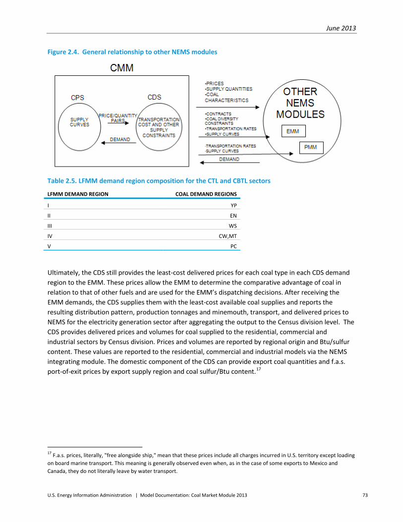
June 2013


Figure 2.4. General relationship to other NEMS modules

Table 2.5. LFMM demand region composition for the CTL and CBTL sectors

LFMM DEMAND REGION COAL DEMAND REGIONS

I YP

II EN

III WS

IV CW,MT

V PC

Ultimately, the CDS still provides the least-cost delivered prices for each coal type in each CDS demand region to the EMM. These prices allow the EMM to determine the comparative advantage of coal in relation to that of other fuels and are used for the EMM’s dispatching decisions. After receiving the EMM demands, the CDS supplies them with the least-cost available coal supplies and reports the resulting distribution pattern, production tonnages and minemouth, transport, and delivered prices to NEMS for the electricity generation sector after aggregating the output to the Census division level. The CDS provides delivered prices and volumes for coal supplied to the residential, commercial and industrial sectors by Census division. Prices and volumes are reported by regional origin and Btu/sulfur content. These values are reported to the residential, commercial and industrial models via the NEMS integrating module. The domestic component of the CDS can provide export coal quantities and f.a.s. port-of-exit prices by export supply region and coal sulfur/Btu content.17

17 F.a.s. prices, literally, "free alongside ship," mean that these prices include all charges incurred in U.S. territory except loading on board marine transport. This meaning is generally observed even when, as in the case of some exports to Mexico and Canada, they do not literally leave by water transport.

June 2013


The CDS also provides detailed input information to the LFMM including transportation rates and coal supply curves. The LFMM uses this information to develop expectations about future coal prices and coal availability and allows the LFMM to determine the economic feasibility of constructing a coal-to-liquids facility by estimating delivered coal prices for specific quantities of coal. In scenarios where allowance prices are modeled (for more information, see section entitled “Environmental Constraints”), allowance prices for SO2 and mercury are sent to the LFMM and are considered in the overall cost of the coal fuel supplied. Emissions from CTL facilities are assumed to be identical to those for IGCC. Additional details of coal-to-liquids modeling are provided in the Liquid Fuels Market Module Documentation.

The output for the domestic component of the CDS falls into two categories:

• Outputs produced specifically for the NEMS system, characteristically in aggregate form and presented in tables that span the forecast period. These reports are primarily designed to meet the output requirements of the Annual Energy Outlook and its Supplement.

• Detailed reports produced in a set for a single forecast year. These reports provide detail on sectoral demands received, regional and national coal distribution patterns, transportation costs, and reporting of regional and supply curves-specific production. Any or all of these reports can be run for any year in the model forecast horizon. These reports are designed to meet requirements for detailed output on special topics, and for diagnostic and calibration purposes.

June 2013


Model Rationale

Theoretical approach Each year, coal is transported from mines to consumers via thousands of individual transportation routes. Subject to certain constraints peculiar to its industrial organization, the behavior of the coal industry is demand-driven and highly competitive. Coal transportation, while far from perfectly competitive in all cases, is a competitive industry when viewed at the national scale. Given this overall picture, it is appropriate to model coal distribution with the central assumption that markets are dominated by the power of consumers acting to minimize the cost of coal supplies. Since the late 1950s, coal supply and distribution has been modeled with this central assumption, using linear programming and/or heuristic solution algorithms that determine the least-cost pattern of supply to meet national demand.

The CDS employs a linear program to determine the least-cost set of supplies to meet overall national coal demand. The detailed pattern of coal production, transportation, and consumption is simplified in the CDS as consisting of about 200 annual demands (the exact number depends on the forecast year and scenario modeled) satisfied from up to 41 coal supply curves.

Constraints limiting the theoretical approach The picture of a highly competitive coal mining industry serving consumers with significant market power is correct, but substantially incomplete. It fails to show powerful constraints on consumer minimization of delivered coal costs that transform the observed behavior of the industry. These major constraints can be categorized:

• Environmental constraints • Technological constraints • Transportation constraints

The deregulation of electricity generation and the increasing uncertainty about the long-term environmental acceptability of coal combustion have combined to remove some of the constraints imposed on coal modeling by long-term contracts and other “security of supply” agreements that tended to reduce the role of cost minimization in domestic coal markets. Environmental regulation and technological inflexibility combine to restrict the types of coal that can be used economically to meet many coal demands, thus reducing the consumer's range of choice. Supply reliability and local limits on transportation competition combine to restrict where, in what quantity, and for how long a technically and environmentally acceptable coal may be available. The synergistic action of these constraints produces a pattern of coal distribution which differs from unconstrained delivered cost minimization.

Environmental constraints

The CMM is capable of modeling compliance with emissions limits established by the Clean Air Act Amendments of 1990 (CAAA90), including the Clean Air Interstate Rule (CAIR) and the Mercury Air Toxics Standard (MATS). In the AEO2013 version of the coal model, the role of modeling these environmental constraints is largely performed by the Electricity Market Module (EMM). Typically, there are three ways in which emission constraints may be met: fuel switching, purchasing emissions

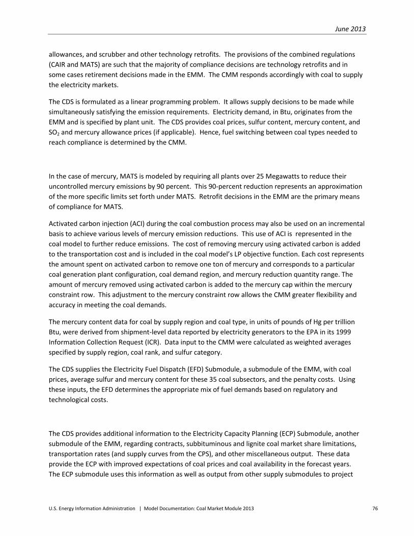
June 2013


allowances, and scrubber and other technology retrofits. The provisions of the combined regulations (CAIR and MATS) are such that the majority of compliance decisions are technology retrofits and in some cases retirement decisions made in the EMM. The CMM responds accordingly with coal to supply the electricity markets.

The CDS is formulated as a linear programming problem. It allows supply decisions to be made while simultaneously satisfying the emission requirements. Electricity demand, in Btu, originates from the EMM and is specified by plant unit. The CDS provides coal prices, sulfur content, mercury content, and SO2 and mercury allowance prices (if applicable). Hence, fuel switching between coal types needed to reach compliance is determined by the CMM.

In the case of mercury, MATS is modeled by requiring all plants over 25 Megawatts to reduce their uncontrolled mercury emissions by 90 percent. This 90-percent reduction represents an approximation of the more specific limits set forth under MATS. Retrofit decisions in the EMM are the primary means of compliance for MATS.

Activated carbon injection (ACI) during the coal combustion process may also be used on an incremental basis to achieve various levels of mercury emission reductions. This use of ACI is represented in the coal model to further reduce emissions. The cost of removing mercury using activated carbon is added to the transportation cost and is included in the coal model’s LP objective function. Each cost represents the amount spent on activated carbon to remove one ton of mercury and corresponds to a particular coal generation plant configuration, coal demand region, and mercury reduction quantity range. The amount of mercury removed using activated carbon is added to the mercury cap within the mercury constraint row. This adjustment to the mercury constraint row allows the CMM greater flexibility and accuracy in meeting the coal demands.

The mercury content data for coal by supply region and coal type, in units of pounds of Hg per trillion Btu, were derived from shipment-level data reported by electricity generators to the EPA in its 1999 Information Collection Request (ICR). Data input to the CMM were calculated as weighted averages specified by supply region, coal rank, and sulfur category.

The CDS supplies the Electricity Fuel Dispatch (EFD) Submodule, a submodule of the EMM, with coal prices, average sulfur and mercury content for these 35 coal subsectors, and the penalty costs. Using these inputs, the EFD determines the appropriate mix of fuel demands based on regulatory and technological costs.

The CDS provides additional information to the Electricity Capacity Planning (ECP) Submodule, another submodule of the EMM, regarding contracts, subbituminous and lignite coal market share limitations, transportation rates (and supply curves from the CPS), and other miscellaneous output. These data provide the ECP with improved expectations of coal prices and coal availability in the forecast years. The ECP submodule uses this information as well as output from other supply submodules to project

June 2013


capital decisions for the electricity markets. In addition to determining new generation capacity, the ECP submodule decides whether to retire coal units or to retrofit existing coal generation units with sulfur dioxide scrubbers. The ECP also estimates sulfur dioxide emissions.

Emissions from coal-to-liquids facilities, which are assumed to generate electricity that is sold to the grid as well as liquid products, are also subject to the restrictions of CAIR and MATS. When applicable, the LFMM adds the cost of allowances to its fuel costs when making its CTL planning decisions. The emissions of CTL plants, similar to IGCC, are low relative to other coal technologies, due to the removal of 99 percent of potential sulfur dioxide and 95 percent of potential mercury emissions. The EMM and the CMM account for the emissions from the coal-to-liquids facilities when evaluating overall compliance with these regulations.

In the other subsectors that do not involve electric power generation, domestic environmental and technical constraints (with their foreign market equivalents for coal exports) combine to restrict choices. These constraints are modeled using the coal groups. In the industrial and residential/commercial sectors, demand is received from other NEMS components in aggregated form and is subdivided into sulfur categories.

Technological constraints

Technological constraints restrict the suitability of coals in different end uses. Coal deposits are chemically and physically heterogeneous; end-use technologies are engineered for optimal performance using coals of limited chemical and physical variability. The use of coals with sub-optimal characteristics carries with it penalties in operating efficiency, maintenance cost, and system reliability. Such penalties range from the economically trivial to the prohibitive, and must be balanced against any savings from the use of less expensive coal.

Precise modeling of the technological constraints on coal cost minimization would require an enormously detailed model, using large quantities of engineering data that are not in the public domain. A simplified approach is adequate for most public policy analyses and is mandated by data availability constraints. Technological constraints on coal choice are simply addressed in the CDS by subdividing sectoral demands into subsectoral detail representing the more important end-use technologies, and by then restricting supplies to these subsectors to one or more of the CMM coal types using the "coal group" definitions. For the electricity sector, the “coal groups” have been relaxed to allow the coal model greater flexibility in satisfying the demands.

June 2013


It is sometimes necessary to restrict regional demands to specific coal sources. In the case of demands for lignite, gob, or anthracite culm, which contains the lowest heat content per ton of the coals modeled in the CMM, transportation over any significant distance creates the double risk of significant Btu loss and spontaneous combustion. In the CDS, such demands can be restricted to demand regions conterminous with the appropriate supply regions.

Again, the advent of deregulation and the increasing importance of electricity generation costs have produced a willingness to overlook some of the less threatening types of damage that can occur from using coals which differ from a boiler’s design specification. Many plants have learned that, with relatively minor investments, newer plants can be easily transferred from bituminous to subbituminous coal. The transportation rate model structure accounts for an increase in expenses when subbituminous coal is used beyond historical levels. (See “Transportation Cost Constraints” below.)

Technical constraints are also represented in the model for certain electricity subsectors and demand regions by modeling diversity constraints for lignite and subbituminous coals. The diversity constraints establish bounds for use of these types of coals. The bounds are established for particular electricity subsector/demand region combinations based on historical patterns of use of lignite and subbituminous coals. Over the forecast, these bounds become considerably less restrictive for subbituminous coals and have all but disappeared for all sectors by 2025. For AEO2013, the lignite diversity constraints either allow plant units within a electricity subsector unlimited use of lignite coal or prevent lignite coal from being used at all.

Transportation cost constraints

Minimization of delivered coal costs may be constrained by the market power of railroads, the dominant transport mode. Railroad rates for coal have historically reflected substantial market power in many regions; they still may in most of the northeastern United States and at locations where alternative coal sources and/or multiple common carriers are lacking.

Nationwide, shipping costs for contract deliveries to electric utilities represented 29 percent of delivered costs in 1984 and only 25 percent in 1987, but amounted to 40 percent of delivered costs to utilities in the South in 1987, and half of delivered costs in the West. 18 In 1999, shipping costs represented about 33 percent of delivered costs to utilities. In some current cases, transport costs have exceeded 80 percent of delivered costs.19 In 1998, coal accounted for 27.3 percent of carloads, 45.5 percent of tonnage, and 22.9 percent of revenue for Class I railroads.20

18 U.S. Energy Information Administration, Trends in Contract Coal Transportation, 1979-1987, DOE/EIA-0549 (Washington, DC, September 1991), p. ix. 19 In 1990 Georgia Power purchased over 1.5 million short tons of Wyoming coal at a delivered cost of $26.48 per short ton, of which the reported minemouth cost at the Caballo Rojo mine in Wyoming was $4.00 per short ton, or 15.1 percent. 20 Association of American Railroads, The Rail Transportation of Coal, January 2000.

June 2013


Coal distribution modeling mandates recognition that coal transportation rates only approach marginal costs of service in the presence of intermodal competition. Further, the difference between cost and price can be significant, not merely on a route-specific basis, but at the national level. Because coal transportation rates may not be determined exclusively by costs or distance, estimation of route-specific transport rates (i.e., when required for topical analyses) is done exogenously. Since thousands of transport routes may be in use in any year, endogenous estimation of a reasonably complete set of route-specific costs would impose unacceptable model execution and maintenance burdens.

In the CDS, domestic transportation rates are inferred by subtracting historical average minemouth prices from historical average delivered prices. Since coal-to-liquids facilities do not currently exist, CTL transportation rates are based upon historical transportation rates to the electricity sector. For each of the 49 subsectors within the six major economic sectors (electric power generation, industrial steam generation, domestic metallurgical production, residential/commercial consumption, coal-to-liquids, and exports), a set of transportation prices connects the 16 demand regions with each of the 41 supply curves. In principle, there are thus 16*41*49=32,144 coal transportation routes and associated prices in the model. In practice, the number of useable routes is substantially less, since many of the origin/destination possibilities represent routes that are economically impractical now and in the foreseeable future.

Alaska produces coal for its own consumption and export, but has never "imported" coal from the contiguous States or overseas. Its only feasible coal transportation connection in the CDS is with the Pacific Northwest region. No other approach is reasonable in such cases, since estimates of transport costs cannot be made for routes that have never been used and where required infrastructure does not exist. A different type of example is provided by the metallurgical coal sector. Not all of the model's supply regions contain coal reserves suitable for making metallurgical coke using current technologies. Similarly, not all demand regions contain coking coal demands. Where there can be neither supply nor demand, coal transportation rates are set to dummy values to prohibit their use. This method allows easy modification of the rates should technological change or economic development produce possibilities where none now exist.

For the electricity sector, an increase over historical volumes for certain transportation routes and coal types may occur in the forecast as generation demand increases and demand changes due to environmental and cost pressures. In certain cases, this incremental volume will require an increase in shipping distance within a demand region. This increase in shipping distance has been reflected in second-tier transportation rates for certain routes. For a plant that has never used coal from a particular supply curve, the model structure provides the capability to model transportation only at a higher second-tier rate.

A higher, second-tier transportation rate is also used for subbituminous coal. This transportation rate is a proxy for the operation costs associated with the use of subbituminous coal, including fouling/slagging, derates, and other production problems that are not currently accounted for in the electricity model. The net effect of the second-tier transportation rate is to add roughly $0.10 per

June 2013


million Btu (measured in 2000 dollars) to the transportation rate for incremental volumes of subbituminous coal.21

Domestic transportation rates in the CDS vary significantly between the same supply and demand regions for different economic sectors. This difference is explained by the following factors:

• Both supply and demand regions may be geographically extensive, but the particular sectoral or subsectoral demands may be focused in different portions of the demand region, while the different types of coal used to meet these demands may be produced in different parts of the supply region.

• Different coal end-uses require coal supplies that must be delivered within a narrow range of particle sizes. Special loading and transportation methods must be used to control breakage for these end uses. Special handling means higher transportation rates, especially for metallurgical, industrial, and residential/commercial coals.

• Different categories of end-use consumers tend to use different size coal shipments, with different annual volumes. As with most bulk commodity transport categories, rates charged tend to vary inversely with both typical shipment size and typical annual volumes.

• Since the Staggers Rail Act of 1980, Class I railroads have been free to make coal transportation contracts that differ in contract terms of service and in the sharing of capital cost between carrier and shipper. Where previously the carrier assumed the expense of providing locomotive power, rolling stock, operating labor and supplies, right-of-way maintenance, and routing and scheduling, more recent "unit train" contracts reflect the use of dedicated locomotive power, rolling stock, and labor operating trains on an invariant schedule. Often the shipper wholly or partly finances these dedicated components of the total contract service. In such cases, the actual costs and services represented by the contract may cover no more than right-of-way maintenance, routing and scheduling. Particular interregional routes may vary widely in the proportion of total coal carriage represented by newer cost sharing and older tariff-based contracts.

21 The estimated cost of switching to subbituminous coal, $0.10/mmBtu, was derived by Energy Ventures Analysis, Inc. and recommended for use in the CMM as part of an Independent Expert Review of the Annual Energy Outlook 2002’s Powder River Basin production and transportation rates.

June 2013


Model Structure The domestic component of the CDS forecasts the quantities of coal needed to meet regionally and sectorally specified coal demands. It provides the Btu and sulfur content of all coal delivered to meet each demand. It also provides annual forecasts of minemouth and delivered coal prices by sector and region. Marginal delivered coal prices by demand sector and plant type are provided to the EMM to be used in formulating regional and sector-specific electricity demands for coal. Additionally, the CDS projects the regional distribution of coal supply by sector, region, mine type, and coal type based on future electricity and non-electricity coal demand. Transportation costs can be summarized independently by coal supply region, coal rank and sulfur content for regional or sectoral transportation analysis. The model code that performs domestic coal distribution tasks in the CMM consists of 15 subroutines, eight sources of input and five output files. The interaction of these components is outlined below and in the accompanying flowcharts.

Computational sequence and input/output flow The controlling submodule in the coal distribution code is called "CDS."22 The functions of subroutine "CDS" are shown in Figure 2.5, which also provides an overview of the operations of the domestic coal distribution code as a whole. "CDS" controls ten other subroutines:

• "CREMTX" creates the linear programming matrix containing the coal demands, supplies, and transport activities. It is called on the first iteration and the first year the model is run.

• "RDCLHIST" reads coal data (minemouth prices, production by supply curve, and regional production) for historical years from the input file, “CLHIST.”

• "CREVISE" revises the linear programming matrix after the initial iteration and calls the linear programming solver, OML, in each forecast year.

• "RETSOL" retrieves the linear program solution produced by OML and sends the appropriate sub-parts of the solution to "INPREP,""DEMREP,""PRDREP,"and "CEXPRT."

• "INPREP" creates the demand reports that record sectoral demands received from other NEMS components and the international component of the CDS. "INPREP" writes output describing the demands it has calculated from the input common block names and physical files described above. Non-electricity and electricity demand reports, plus an electricity demand summary report, are written to the physical file "CLCDS." These reports appear at the head of the year-specific detailed CDS output that consists of approximately 17 reports available for each forecast year. Using these reports it is possible to determine exactly what demands the CDS has solved for in a given forecast year, since this output is written before the linear program is called by the "CDS" subroutine.

22To avoid confusion in the following discussion, subroutine and file names are always written in quotation marks, e.g., "CDS", "EMMOUT."

June 2013


• "DEMREP" generates coal demand reports that describe demand, transportation, and distribution of coal from supply to demand region by economic sector, with fully adjusted transport rate data provided in both dollars per ton and dollars per million Btu. One of these year-specific reports, the "Detailed Supply and Price Report," provides a full description of coal type, demand quantity, individual participants, and minemouth, transportation, and delivered costs for an entire run, in the order of the 16 domestic CDS demand regions. This is the most detailed report currently available from the CDS, and generally requires 30 to 50 pages per forecast year (divided into 14 regional subreports). Reports generated by "DEMREP" are written to the physical file "CLCDS."

• "PRDREP" generates coal production reports that describe the quantities of coal produced by coal type from each coal supply curve in each supply region. Accompanying production quantities in millions of tons are associated minemouth prices. The definition for each coal type that is assigned to individual coal supply curves defines a sulfur and Btu category, but values of sulfur and Btu that are specific to each supply curve (and which are taken from the EIA 923) are also available, and are used by both the CDS and the EMM to calculate precise dollars per million Btu prices and sulfur contents (in lbs of sulfur per million Btu). The coal production reports are written on physical file "CLCDS".

• "CEXPRT" generates reports from the export portion of the linear program. • "CPSHR" writes non-electric coal price output to the common block name "PQ," and

delivered coal prices, sulfur and Btu assignments for coals assigned to electricity demands to the common block name "COALOUT." "CPSHR" writes prices, sulfur, and Btu content for coal meeting electricity demands to a physical file named "CLCDS." As the name implies, "CLDEBUG" contains output describing the iteration-by-iteration output of the CDS that is used in resolving problems that arise in the operation of the CMM and/or other NEMS models with which it interacts.

• "CBFOUT" is called both directly from the subroutine “CDS” and also from “RDCDSIN” and calculates Btu conversion factors, an important process since the Coal Market Module mimics actual industry behavior in modeling the mining and shipping of coal in short tons, but demands are met in terms of least delivered cost per million Btu. This conversion is conceptually important since production, transportation, and delivery data are required to be reported in both physical units and trillion Btu. The conversions accomplished in "CBFOUT" are reported to the common block name "COALOUT."

The subroutine "CDS" calls the above subroutines in the same order in which they are discussed above. Subroutine "CREMTX" also calls other subroutines "RDCDSIN," "RDCEXIN," "RCMMDB,""COALDEFS," and "WRCINDB" (Figure 2.6):

• "RDCDSIN" reads input files containing calibration factors for the CDS, and calls "CMAPSR," "CDSINT," and "CBFOUT."

• "RDCEXIN" reads input files containing calibration factors for the international portion of the CDS. These inputs are described in Section 3 - Coal Distribution Submodule -International Component, Appendix 3.C.

June 2013


The subroutine "CDSINT" called by subroutine "RDCDSIN" initializes all arrays and reads input data from four physical files. These input units are as follows:

• CLPARAM" which contains parameters that order the assignment of demands, assign coal type labels and sectoral names, and provides important adjustments to minemouth and transportation prices, as well as constraining the types of coal that can be used to fill demands in different economic sectors and regions. (The contents of "CLPARAM" and other physical input files are described in greater detail in Appendix 2.C of this report.)

• "CLNODES" contains supply and demand region name labels. • "CLRATES" contains a large matrix of transportation rates defined by economic subsector,

coal supply, and demand regions. These rates are specified in 1987 dollars and are adjusted to provide rates in the dollar year used in any run, as well as adjustments specific to the economic sector and forecast years. These last two adjustments are accomplished by parameters found in "CLPARAM" that are discussed in Appendix 2.C.

• "CLCONT" contains data defining electricity coal distributions that are assigned to constrain the selection of coal sources by the CDS solution algorithm. Beginning with AEO2005, a modification was made so that these minimum flows are able to follow a plant unit even if it upgrades (acquiring new emission control equipment). This data file also contains profiles associated with each plant, defining its transportation rate structure and its ability to use subbituminous and lignite coals. The nature of this input and its use is also discussed in Appendix 2.C.

The "CMAPSR" subroutine creates the regionally and sectorally distinct demands for which the CDS solves. It does not, however, prioritize these demands, nor does it perform the important step of modifying the demands to reflect the constraints imposed by existing electricity coal contracts. Both these processes are accomplished by subroutine "CREMTX," which is described in association with the discussion of Figures 2.5 and 2.6. "CMAPSR" reads common block names "PQ" (which contains the non-electricity coal demands) and the physical file "CLSHARE" (which contains the shares disaggregating non-electricity demands from Census division to CDS demand region level).

June 2013


Figure 2.5. Structure pf CDS subroutines – overview*

June 2013


Figure 2.6. Functions of subroutine – “CREMTX”

Key computations and equations The CDS uses a linear programming (LP) formulation to find minimum-cost coal supplies to meet domestic sectoral coal demands received from the Electricity Market Module, the Residential, Commercial and Industrial Demand Modules, and international demands as determined in the international component of the CDS. The linear program for the domestic component of the CDS selects the coal supply sources for all coal demands in each domestic CDS demand region, subject to the constraint that all demands are met.

The domestic component of the CDS orders input data, solves the LP model, and provides the required outputs to the CPS and to other modules of the NEMS. The initial matrix and objective function are inputs. However, most of the coefficients in the model change over time. For example, the objective function represents the cost of delivering coal from supply regions to demand regions, and its coefficients include minemouth prices, transportation rates and coal demands specified by heat and sulfur content, all of which may vary. Similarly, coefficients in the constraint matrix, which include the electricity coal contracts, also change within the forecast horizon. Appendix 2.B provides mathematical descriptions of the objective function and equations of the constraint matrix, and of the equations that derive the revised coefficients for the LP model. Appendix 2.C describes model inputs, parameter estimates and model output. Appendix 2.D describes data quality and estimation. The model relies on Optimization and Modeling Library (OML) software, a proprietary mathematical programming package,

June 2013


to create and store coefficients in a database, solve the problem, and retrieve the solution. The OML subroutines are summarized in Appendix 3.E of Section 3 of this documentation report.

Transportation rate methodology Inter-regional coal transportation rates are calculated exogenously and read by subroutine "CDSINT" from the physical file "CLRATES." "CLRATES" contains rates for each possible combination of 49 economic subsectors, 16 demand regions and 41 supply curves. The input rate array contained in "CLRATES" is prepared by subtracting minemouth prices from the EIA Form 7A, "Coal Production Report" from sector-specific delivered prices from the Form EIA-3, “Quarterly Coal Consumption and Quality Report, Manufacturing and Transformation/Processing Coal Plants and Commercial and Institutional Users” (for the industrial steam and residential/commercial sectors), from the Form EIA-5, "Quarterly Coal Consumption and Quality Report, Coke Plants" for the domestic coking coal sector, from the Form EM-545 for coal exports, and from the EIA-923, “Power Plant Operations Report” for the electricity sector.

For the electricity sector only, a two-tier transportation rate structure is used for those regions which, in response to rising demands or changes in demands, may expand their market share beyond historical levels. The first-tier rate is representative of the historical average transportation rate. The second-tier transportation rate is used to capture the higher cost of expanded shipping distances in large demand regions. The second tier may also be used to capture costs associated with the use of subbituminous coal at units that were not originally designed for its use. This cost is estimated at $0.10 per million Btu (2000 dollars).

Coal transportation costs, both first- and second-tier rates, are modified over time by two regional (East and West) transportation indices. The indices are measures of the change in average transportation rates, on a tonnage basis, that occurs between successive years for rail and multi-mode coal shipments. An East index is used for coal originating from eastern supply regions while a West index is used for coal originating from western supply regions. The indices are calculated econometrically as a function of railroad productivity, the user cost of capital of railroad equipment (East only), investment (West only), diesel fuel price (East only), and the western share of national coal demand (West only). Although the indices are derived from railroad information, they are universally applied to all coal transportation rates within the CMM. In the AEO2013 reference case, both eastern and western coal transportation rates are projected to remain near their 2011 levels through 2040. See Appendix 2.D for more information regarding the methodology and assumptions used to derive the transportation rate indices.

For the case of increased shipping distances, the second-tier transportation rate is calculated by assuming a geographic centroid for the relevant demand region, estimating an approximate distance, and where possible using ton-mile data from the FERC Form 580, “Interrogatory on Fuel and Energy Purchase Practices,” to calculate a new dollars-per-ton transportation rate. For subbituminous coals,

June 2013


$0.10 per million Btu (2000 dollars) is assumed to be, on average, representative of the added difficulty of using subbituminous coal.23 These difficulties include slagging/fouling problems, impacts on heat rates, and other operation costs. For subbituminous coals, the second-tier rate is simply the first-tier rate plus this adder of $0.10 per million Btu. For certain supply/demand region pairs, the second-tier rate may include both the $0.10 per million Btu adjustment as well as a geographic adder.

23 $0.10/mmBtu, the estimated cost of switching to subbituminous coal, was derived by Energy Ventures Analysis, Inc., and recommended for use in the CMM as part of an Independent Expert Review of the Annual Energy Outlook 2002’s Powder River Basin production and transportation rates. Barbaro, Ralph and Seth Schwartz. Review of the Annual Energy Outlook 2002 Reference Case Forecast for PRB Coal, prepared for the U.S. Energy Information Administration (Arlington, VA: Energy Ventures Analysis, Inc., August 2002)

June 2013


Appendix 2.A. Submodule Abstract Model name: Coal Distribution Submodule -Domestic Component

Model abbreviation: CDS

Description: United States coal production, national coal transportation industries.

Purpose: Forecasts of annual coal supply and distribution to domestic markets.


Part of another model:


Model interface: The model interfaces with the following models: within the Coal Market Module, the CDS interfaces with the Coal Production Submodule. Within NEMS, the CDS receives industrial steam and metallurgical coal demands from the NEMS Industrial Demand Module, coal-to-liquids demands from the NEMS Liquid Fuels Market Module, residential demands from the NEMS Residential Demand Module, commercial demands from the NEMS Commercial Demand Module, and electricity sector demands from the NEMS Electricity Market Module. The CDS also receives macro-economic variables from the NEMS Macro-Economic Activity Module.


Office: Electricity, Coal, Nuclear and Renewables Analysis Division: Coal and Electric Power Model Contact: Diane Kearney Telephone: (202) 586-2415 E-mail: Diane Kearney (diane.kearney@eia. gov)

Documentation:

• Energy Information Administration, Model Documentation, Coal Market Module of the National Energy Modeling System, DOE/EIA-M060(2013) (Washington, DC, June 2013).

• U.S. Energy Information Administration, Overview of the Coal Market Module of the National Energy Modeling System, April 1992.

Archive media and installation manual: NEMS13 - Annual Energy Outlook 2013.

Energy system described by the model: Coal demand distribution at various demand regions by demand

June 2013


Coverage:

• Geographic: United States, excluding Puerto Rico, and the U.S. Virgin Islands. • Time unit/Frequency: 2003 through 2040 (with structure available through 2050) • Basic products involved: Bituminous, subbituminous and lignite coals in steam and

metallurgical coal markets. • Economic Sectors: Forecasts coal supply to two residential/commercial, three industrial,

two domestic metallurgical, one coal-to-liquids, six export, and 35 electricity subsectors to 16 domestic demand regions.

Special features:

• All data on demands are exogenous to the CDS. • Supply curves (there are 41 supply sources) depicting coal reserve base are exogenous to

CDS and are reported in the CDS from 14 coal supply regions. • CDS currently contains no descriptive detail on coal transportation by different modes and

routes. Transportation modeling consists only of sector-specific rates between demand and supply curves that are adjusted annually for factor input cost changes.

• CDS output includes tables of aggregated output for NEMS system and approximately six single-year reports providing greater regional and sectoral detail on demands, production distribution patterns, and rates charged.

• Coal imports are calculated endogenously. • CDS reports minemouth, transport and delivered prices, coal shipment origins and

destinations (by region and economic subsector), coal Btu and sulfur levels.

Modeling features:

• Structure: The CDS uses 41 coal supply sources representing 12 types of coal produced in 14 supply regions. Coal shipment costs to consumers are represented by transportation rates specific to NEMS sector and supply curve/demand region pair, based on historical differences between minemouth and delivered prices for such coal movements. In principle there are up to 31,360 such rates for any forecast year; in practice there are less since many rates are economically infeasible and a unique transportation rate is not derived for each of the 35 electricity sectors. Coal supplies are delivered to up to 49 demand subsectors in each of the 16 demand regions. A single model run represents a single year, but up to 33 consecutive years (2003-2040) may be run in an iterative fashion. Currently, the NEMS system provides demand input for the 1990-2040 period. (Note: many of the input files have been structurally extended to 2050, but assumptions about activity between 2040 and 2050 are not considered valid.)

• Modeling technique: The model utilizes a linear programming that minimizes the estimated delivered cost to all demand sectors.

June 2013


• Model interfaces: The NEMS residential, commercial, and industrial models provide estimates of coal demand for those sectors, while the NEMS Liquid Fuels Market Module provides demands for the coal-to-liquids sector, and the NEMS Electricity Market Module provides demands for the electricity generation sectors. The CDS provides the NEMS with coal production estimates, Btu conversion factors, and estimated minemouth, transportation and delivered costs for coal supplies to meet the demands. The CDS interfaces with the international component of the CDS to receive coal export demands. The CDS interfaces with the Coal Market Module's Coal Production Submodule to receive supply curves that specify the minemouth price in relation to the quantity demanded. In turn, the CPS receives production quantities from the CDS that are used to revise its prices, if necessary, for subsequent iterations.

Physical:

• Demand shares by sector and region: (1) residential/commercial (trillion Btu); (2) industrial steam coal (trillion Btu): (3) industrial metallurgical coal (trillion Btu); (4) industrial coal-to-liquids (trillion Btu) (5) import supplies (millions of short tons)

• Coal contracts for electricity sector: (1) coal demand regions; (2) supply regions; (3) coal quality (Btu and sulfur content); (4) contract historical volumes (trillion Btu); (5) contract profiles for each forecast year

• Coal quality data for supply curves: (1) million Btu per short ton; (2) lbs sulfur per million Btu; (3) lbs. of mercury per trillion Btu; (4) lbs. of carbon dioxide emitted per million Btu

• Coal quality specifications for regional subsectoral demands in electricity generation and other sectors

Economic:

• Supply curves relating minemouth prices to cumulative production levels • Transportation rates: (1) 1987 dollars per short ton; (2) specified by subsector, differ by

sector; (3) differ also by supply curve and demand region pair • Transportation rate escalation factors: (1) endogenous; (2) regional (eastern and western

railroads); (3) based on estimates of railroad productivity, the producer price index for rail equipment, contract duration, and distance (for western railroads only); (4) used to escalate and de-escalate transportation rates by forecast year

• Minemouth price adjustments: (1) can be made by supply region and forecast year; (2) currently used only by forecast year; (3) used to adjust for productivity change

• Transportation rate adjustments (not used in AEO2013): (1) can be used by demand sector and demand region; (2) derived from off-line program that subtracts base-year minemouth costs from delivered costs reported in Forms EIA-3 and -5, and 923 to produce transport rate, calculates ratio between model rate and rate from forms, preserve ratio as model parameter; (3) used to calibrate rates in model

June 2013


Data sources:

• Form EIA-3, "Quarterly Coal Consumption and Quality Report, Manufacturing and Transformation/Processing Coal Plants and Commercial and Institutional Users "

• Form EIA-5, "Quarterly Coal Consumption and Quality Report, Coke Plants" • Form EIA-7A, "Coal Production and Preparation Report" • FERC Form 423, "Monthly Report of Cost and Quality of Fuels for Electric Plants" • Form EIA-423, “Monthly Cost and Quality of Fuels for Electric Plants Report” • Form EIA-923, “Power Plant Operations Report” • FERC Form 580, "Interrogatory on Fuel and Energy Purchase Practices" • U.S. Department of Commerce, Form EM-545 • U.S. Department of Commerce, Form IM-145 • Association of American Railroads, AAR Railroad Cost Indices (Washington, DC, quarterly) • Rand McNally and Co., Handy Railroad Atlas of The United States (Chicago, IL, 1988) • Caplan, Abby, et al, eds., 1996-1997 Fieldston Coal Transportation Manual (Washington, DC,

1996)

Output data:

• Physical: Forecasts of annual coal supply tonnages (and trillion Btu) by economic sector and subsector, coal supply region, coal Btu, coal sulfur content, coal mercury content, and demand region

• Economic: Forecasts of annual minemouth, transportation and delivered coal prices by coal type, economic sector, coal demand and supply regions


Inhouse or proprietary:

Inhouse


Independent expert reviews were conducted for the Component Design Report, which was reviewed by Dr. Charles Kolstad of the University of Illinois and by Dr. Stanley Suboleski of the Pennsylvania State University during 1992 and 1993.

An independent expert review was conducted in 2002 by PA Consulting Group and Energy Ventures Analysis, Inc. The focus of the review was on forecasted levels of production supplied from the Powder River Basin and transportation rates. Some of the recommendations were incorporated into the Annual Energy Outlook 2003. As a result of the review, some transportation rates were re-estimated, a two-tier transportation rate structure was introduced, and two coal demand regions were redefined. The coal demand regions that were redefined included MT and ZN. Previously, Nevada, Colorado, and Utah were included in MT. The change included adding these states to ZN.

June 2013


In 2003, PA Consulting Group and Energy Ventures Analysis, Inc. were asked to review the entire coal forecast of the Annual Energy Outlook 2003. Based on their recommendations, an additional coal demand region, CU, was added for the Annual Energy Outlook 2004 which includes Colorado, Utah, and Nevada.

Status of evaluation efforts conducted by model sponsor: No formal evaluation efforts other than the above reviews have been made at the date of this writing.

Last update: The CDS is updated annually for use in support of each year’s Annual Energy Outlook. The version described in this abstract was updated in October 2012.

June 2013


Appendix 2.B. Detailed Mathematical Description of the Model The CDS model is specified as a Linear Program (LP) in which the total costs of coal supply, including production, transportation, and the cost of satisfying environmental constraints, are minimized. The CDS receives production costs iteratively from the CPS. These production costs are limited in scope to the neighborhood of the solution. The iterative relationship between the CPS and the CDS allows non-linear supply curve information calculated in the CPS to be approximated by a linear form in the CDS. Costs of transportation from supply to demand regions are added to the production costs. The costs of limiting sulfur dioxide emissions and other pollutants for certain scenarios (i.e., mercury and carbon dioxide) can be modeled in the cost minimization LP. Based on these total costs, the model calculates the optimum pattern of supply required to satisfy demand.

Mathematical formulation

The table of column activity definitions and row constraints defined in the CDS linear program incorporates assumptions described in Model Rationale in Section 2 and variable definitions that are described in Appendix 2.C in Table 2.C-1. The general structure of the LP matrix is shown as a block diagram in Table 2.B-1.

The block diagram format depicts the matrix as made up of sub-matrices or blocks of similar variables, equations, and coefficients. The first column in the diagram contains descriptions of the rows of equations in the model. The subsequent columns define sets of variables for the production and transportation of coal. Other columns are necessary to represent contracts, coal diversity constraints, SO2, mercury, and carbon dioxide constraints. Contracts represent binding agreements between coal suppliers and generators. Coal diversity constraints represent technical constraints limiting the use of certain types of coal within particular plant types in certain demand regions. These constraints are currently limited to the use of subbituminous and lignite coals. Environmental constraints represent caps that may be present in certain scenarios. The columns referencing activated carbon define certain specialized activities in which activated carbon may be used by power generators to reduce emissions of mercury. The activated carbon features are only used in scenarios where a mercury regulation is in place, such as when modeling the effects of the Mercury Air Toxics Standard (MATS).

The various rows of the matrix include the objective function, the demand, production, contracts, diversity, sulfur, mercury, carbon, and activated carbon rows. The objective function row, which is considered a free row, is set up as a linear programming cost minimization problem. Other free rows, used to collect information from the model solution, are present in the LP structure but are not depicted in the diagram below. However, they are described in the section titled, “Row and Column Structure of the Coal Market Module” within this appendix. The column labeled Row Type shows the equations to be maximums, minimums, or equalities. Each block within the table is shown with representative coefficients for that block. These coefficients are applied to the quantities (typically in trillion Btu) specified by their column intersections. The last column labeled RHS contains symbols that represent the physical limitations such as supply capacities, demands, or minimum flows.

June 2013


The CDS matrix currently contains about 6,900 rows (equations) and 35,000 columns (activities). The block diagram in Table 2.B-1 is a way of showing the matrix structure in a single table. The coefficients represented in the rows of the matrix as shown in the Table 2.B-1 are applied to the quantities of coal solved for by the model.

The mathematical specification for the CDS optimization program incorporates within its structure the optimization program for international coal flows, which is discussed in Section 3 of this document.

June 2013


Table 2.B-1. CDS linear program structure—domestic component

PRODUCTION

REGIONAL TRANSFER

MERC. PRICE CAP

ESCAPE VECTOR

CARBON VECTOR

EMISSION VECTOR

Row Type RHS

MASK P(SR)(U)(M)(S)SCRUB: F(SR)(DR)X(C)

UNSCRUB.: C(SR)(DR)X(C) DSS(DR)(PT) DSL(DR)(PT)

MVS(DR1)(DR2) MERCEV* MOREHGXX

ACIXSS (ACSTEP)Y CARBONXX

COAL RANK SUB LIG OTHER SUB LIG OTHER SUB LIG

SECTOR ELEC. ELEC. ELEC. ELEC. ELEC. ELEC. CTL Other

TIER ELEC ELEC. ELEC. ELEC. ELEC. ELEC. ELEC. ELEC. ELEC. ELEC.

Objective +p +t0 +t0 +t0 +t1 +t1 +t1 +t2 +t2 +t2 +9.9 +9.9 +15 +15 + CAP +20 +v +EMETAX -- MIN

Demand:

D.(DR)(PT) +1 +1 +1 +1 +1 +1 EQ D

D.(DR)(SEC) +1 +1 EQ D

Contracts:

SCRUBBED: F(SR)(DR)X(C) +1 +1 +1 +1 +1 +1 -1 GE B1

UNSCRUBBED: C(SR)(DR)X(C) +1 +1 +1 +1 +1 +1 -1 GE B2

Production: S@(SR)(U)(M)(C) +1 -1 -1 -1 -1 -1 -1 EQ 0

Productive Capacity: X@(SR)(U)(M)(C) +1 LE PCAP

Diversity Rows: DVS(DR)(PT) +1 +1 -1 LE B3

Lignite: DVL(DR)(PT) +1 +1 -1 LE B4

Transportation: T(SR)(DR)(C) +1 +1 +1 +1 +1 +1 -1 LE TSulfur Dioxide: SULFPEN1 and SULFPEN2 +s +s +s +s +s +s LE S

SULFPN(DR1) +s +s +s +s +s +s-s or +s,

depending LE Sr

MVSO2(DR2) +s +s +s +s +s +s-s or +s,

depending LE Strade

Mercury: MERCP01 +m +m +m +m +m +m -1 -1 LE M ACIXXXXY +a +a +a -10 LE 0

Carbon: CARBONXX +c +c +c +c +c +c -1 EQ 0

1(SR)(U)(M)(R)(DR)(PT)(C) (ACSTEP)(SR)(U)(M)(R)(DR)(PT)(C) T(SR)(U)(M)(R)(DR)(SEC)(C)

Transportation Vectors

Coal Distribution Submodule Block Diagram

1ST TIER 1ST TIER W/ ACTIV CARBONCONTRACT ESCAPE

VECTORS DIVERSITY ESCAPE VECTORS

June 2013


Objective function

The objective of the LP is to minimize delivered costs of coal, including the costs associated with moving coal from supply regions to demand regions. The objective function below defines the costs being minimized by the CDS. The costs include production, transportation, activated carbon (mercury scenarios), costs associated with a mercury cap (specific mercury scenarios), carbon (carbon scenarios), and escape vector costs. Activated carbon costs are relevant in mercury scenarios where activated carbon is injected during the coal combustion process in order to achieve various levels of mercury emissions reduction. In certain scenarios where a mercury allowance price is constrained, a mercury cap cost is included in the LP objective function. The presence of a volume in the mercury cap cost column indicates that the allowance price calculated by the coal LP is higher than the mercury cap. The cost associated with carbon emissions is only relevant in carbon scenarios. This cost is included in the objective function to allow the coal model’s regional distributions to be influenced when carbon limits are present. Escape vectors are a mechanism to allow the model to ignore a constraint by paying a large penalty. Escape vectors are a useful tool in identifying errors in assumptions or conflicting constraints and do not represent the true cost associated with coal deliveries. Iteratively, the escape vectors assist in gently pushing the model towards a feasible solution. When a feasible solution is obtained, the escape vectors are no longer active. The objective function is defined as:

Σi,r,t,u,s [Qpi,r,s,t,u * Pi,r,s,t,u] + Σi,j,p,r,t,u,v [Qt i,j,p,r,t,u,v * Ti,j,p,r,t,u,v] + Σi,j,k,r,t,u [Q2t i,j,k,r,t,u * Ti,j,k,r,t,u] +

Σv [Av * xv] + [H * y] + [C * z] + escape vector costs (2.B-1)

where the indexes are defined as follows:

Index Definitions

Index Symbol Description (i) Coal supply region (j) Coal demand region (k) Demand subsector (p) Plant configuration (index p is a subset of index k) (r) Coal rank (s) Supply curve step (t) Mine type (u) Sulfur level (v) Activated carbon supply curve step (w) Scrubbed or unscrubbed electricity plant type

June 2013


where the columns are defined as:

Column definitions

Column Notation Description

Qpi,r,s,t,u = Quantity of coal from step s of the supply curve produced from coal supply region i, of sulfur level u, mine type t, and rank r. Corresponds to Block Diagram Column: P(SR)(U)(M)(S).

Qti,j,p,r,t,u,v = Total quantity of coal transported from all steps of coal supply region i to coal demand region j, of sulfur level u, rank r, and mine type t, for the electricity plant type p, and activated carbon step v (if relevant to scenario).

Corresponds to Block Diagram Columns: 1(SR)(U)(M)(R)(DR)(PT)(C) and (ACSTEP)(SR)(U)(M)(R)(DR)(PT)(C)

Q2ti,j,k,r,t,u = Total quantity of coal transported from all steps of coal supply region i to coal demand region j, of sulfur level u, rank r, and mine type t, for the demand subsector k for the non-electricity sectors or

Total quantity of coal transported at 2nd tier transportation rate from all steps of coal supply region i to coal demand region j, of sulfur level u, rank r, and mine type t, for the demand subsector k for the electricity sector

Corresponds to Block Diagram Columns: T(SR)(U)(M)(R)(DR)(PT)(C)

Av = Total quantity of activated carbon from activated carbon supply

curve step v.

Corresponds to Block Diagram Column: ACIXSS(ACSTEP)Y

H = Quantity of mercury getting mercury cap price (only relevant for specific mercury scenarios) Corresponds to Block Diagram Column: MERCEV

C = Quantity of carbon emitted from coal

June 2013


And the incremental costs assigned to the column vectors are defined as:

P = Production or minemouth price T = Transportation price (plus cost of activated carbon, if relevant to scenario) x = Cost of activated carbon y = Mercury allowance price cap z = Carbon tax

The escape vector costs correspond to the costs associated with the columns: F(SR)(DR)X(C), C(SR)(DR)X(C), DSS(DR)(PT), DSL(DR)(PT), and MOREHGXX. These costs are high so that they are chosen only as a last resort in order to keep the model feasible. By assisting in maintaining feasibility in early model runs, the linear supply curves can be moved along the supply functions in search of an optimal, minimum cost solution that is feasible without the escape vectors.

Row constraints

The rows interact with the columns present in the objective function to define the feasible region of the LP and are defined below.

SUPPLY BALANCE EQUATIONS: For specific i,r,t,and u: ΣsQpi,r,s,t,u - Σj,k,v Qti,j,k,r,t,u,v = 0 (2.B-2) DEFINITION: Balance the coal produced from each supply region with the coal transported. CORRESPONDING ROW IN BLOCK DIAGRAM: S@(SR)(U)(M)(C)

PRODUCTIVE CAPACITY LIMIT CONSTRAINTS: For specific i,r,t,and u: ΣsQpi,r,s,t,u ≤ PCAPi,r,t,u (2.B-3) DEFINITION: Prevents coal production by supply curve from exceeding its productive capacity limit (PCAP). CORRESPONDING ROW IN BLOCK DIAGRAM: X@(SR)(U)(M)(C)

DEMAND BALANCE EQUATIONS: For specific j and k: Σi,r,t,u,vQti,j,k,r,t,u,v = Dj,k (2.B-4) DEFINITION: Balance the coal transported with the coal demanded by coal demand region and subsector. CORRESPONDING ROWS IN BLOCK DIAGRAM: D.(DR)(PT) and D.(DR)(SEC)

June 2013


CONTRACT FLOWS CONSTRAINTS: For specific i, j, r, t, u: Σp,v,wQti,j,p,r,t,u,v,w – escape vector quantity ≥ Bi,j,r,t,u,w , (2.B-5) where “B” equals contract quantity and “w” indicates whether plant type p is scrubbed or unscrubbed. DEFINITION: Require minimum quantities of coal, “B,” of a specific coal quality from particular supply regions to satisfy electricity contracts from particular demand regions for scrubbed and unscrubbed plants. CORRESPONDING ROWS IN BLOCK DIAGRAM: F(SR)(DR)X(C) and C(SR)(DR)X(C)

DIVERSITY REQUIREMENTS CONSTRAINTS: For a specific j, p, and r (subbituminous or lignite only), where “B” equals subbituminous or lignite coal limit: Σi,t,u, Qti,j,p,r,t,u ≤ Bj,p,r (2.B-6)

DEFINITION: Limits the amount of subbituminous and lignite coal used to satisfy demand in certain electricity demand subsectors and regions. CORRESPONDING ROWS IN BLOCK DIAGRAM: DVS(DR)(PT) and DVL(DR)(PT)

TRANSPORTATION RATE RESTRICTIONS CONSTRAINTS: Σp(Qti,j,p,r,t,u – Qt2i,j,p,r,t,u) ≤ T i,j,r,t,u (2.B-7) DEFINITION: Limits the amount of coal that may be transported at rates applicable to historical flow levels for the electricity sector for a specific i, j, p, r, u, and t, where “T” is the amount of coal capable of being transported at the current rates (first tier rates). Additional transportation flows are assumed to require additional cost (second tier rates) in order to expand coal deliveries in these regions. CORRESPONDING ROW IN BLOCK DIAGRAM: T(SR)(DR)(PT)(C)

SULFUR DIOXIDE EMISSION RESTRICTIONS CONSTRAINTS: sulfur dioxide emissions from imports + Σi,j,p,r,t,u [si,r,t,u* Qti,j,p,r,t,u] ≤ S (2.B-8) DEFINITION: For relevant years, restrict the sulfur levels of coal in the electricity sector such that the sulfur dioxide emissions limit is met, where “s” equals the sulfur dioxide content of the coal and “S” equals the emissions limit. For more detail on sulfur dioxide emissions from imports, see “3. Coal Distribution submodule – International Component.” CORRESPONDING ROW IN BLOCK DIAGRAM: SULFPEN1 and SULFPEN2

SULFUR DIOXIDE EMISSION REGIONAL LIMITS CONSTRAINTS (for CSAPR): sulfur dioxide emissions from imports + Σi,j,p,r,t,u [si,r,t,u* Qti,j,p,r,t,u] -/+ MVS(DR1)(DR2) ≤ Sr (2.B-9) DEFINITION: For relevant years, restrict the sulfur levels of coal in the electricity sector such that the sulfur dioxide emissions limit is met regionally, where “s” equals the sulfur dioxide content of the coal

June 2013


and “Sr” equals the regional emissions limit. A negative MVSO2(DR1)(DR2) represents the amount of sulfur dioxide emissions produced in demand region 1 (DR1) but can be credited to (DR2). A positive MVSO2(DR1)(DR2) represents the amount of sulfur dioxide emissions though produced in demand region 2 (DR2) but can be credited to DEMAND region (DR1). CORRESPONDING ROW IN BLOCK DIAGRAM: SULFPN(DR1)

SULFUR DIOXIDE REGIONAL TRADE (for CSAPR) sulfur dioxide emissions from imports + Σi,j,p,r,t,u [si,r,t,u* Qti,j,p,r,t,u] ≤ Strade (2.B-10) DEFINITION: For relevant years, restrict the trade of sulfur allowances, where “s trade” equals the maximum amount of sulfur dioxide emissions that can be credited to a different region other than where the emissions were produced. CORRESPONDING ROW IN BLOCK DIAGRAM: MVSO2(DR2)

MERCURY EMISSION RESTRICTIONS CONSTRAINTS: Σi,j,k,r,t,u [mi,r,t,u * Qti,j,k,r,t,u] – H – escape vector quantity ≤ M (2.B-11) DEFINITION: Limits the quantity of mercury present in coal (adjusted with the plant removal rate and use of activated carbon) to be less than or equal to the coal mercury emissions limit, “M.” Coefficient mi,,t is the mercury content of coal. Some mercury scenarios cap the compliance costs. In these scenarios, additional “allowances” are available at the allowance cap. “H” is the volume of additional allowances purchased at the cap price. Escape vectors are not active in the final solution but allow feasibility to be maintained in early iterations. CORRESPONDING ROW IN BLOCK DIAGRAM: MERCP01

ACTIVATED CARBON SUPPLY CURVE CONSTRAINTS: Σi,j,p,r,t,u,v [ap,v* Qti,j,p,r,t,u,v] – 10 * Σ v Av ≤ 0 (2.B-12) DEFINITION: Balances the activated carbon used in association with the electricity sector transportation vectors with the activated carbon supply curves. Coefficient ap,v represents tons of activated carbon per trillion Btu for plant configuration p and activated supply curve step v. “Av” represents the total quantity of activated carbon from activated carbon supply curve step v. CORRESPONDING ROW IN BLOCK DIAGRAM: ACIXXXY

CARBON TAX CONSTRAINTS: Σi,j,p,r,t,u [ci,j,p,r,t,u* Qti,j,p,r,t,u] – C ≤ 0 (2.B-13) DEFINITION: Balances the carbon emissions, “C,” associated with the electricity sector transportation vectors with the carbon emissions being “paid for” with the carbon penalty price. The coefficient ci,j,p,r,t,u

represents the carbon content of coal. CORRESPONDING ROW IN BLOCK DIAGRAM: CARBONXX

Output Variables

June 2013


Xi,j,k,r,t,u,v = Quantity of coal rank r, sulfur level u, and mine type t that is transported from coal supply region i to coal import region j for coal demand sector k and activated carbon step v (if relevant to the scenario).

Ui,k,t = Finalized (solution) delivered price (minemouth plus transportation cost) of coal from mine type t to demand sector k in demand region j. This variable is the final optimized value from the CDS.

Each column and row of the linear programming matrix is assigned a name identifying the activity or constraint that it represents. A mask defines the general or generic name of a set of related activities or constraints. For example, the mask ‘P(SR)(R)(U)(M)(SP)’ defines the general name of all activities representing the production of coal. The names of specific activities or constraints are formed by inserting into the mask appropriate members of notational sets identified by the mask. For instance, the production of coal in Northern Appalachia, of bituminous rank, of low sulfur content, from underground mines, and from existing mines (step 1 of a supply curve) is represented by the column vector P(NA)(B)(C)(U)(1).

June 2013


Table 2.B-2. Row and column structure for the domestic component of the coal market module

MASK ROW OR COLUMN ACTIVITY REPRESENTED

ACIXSS(ACSTEP)Y Column

Volume of activated carbon (in lbs) injected to reduce mercury emissions; column bounds on this vector are present specifying how much activated carbon is available at each step

ACIXXXXY Row

Assigns activated carbon requirement (lbs of activated carbon per trillion Btu) for each activated carbon step in transportation column

(ACSTEP)(SR)(U)(M)(DR)(PT)(C) Column

Volume of coal transported in association with the use of activated carbon for particular activated carbon supply curve step (ACSTEP), from supply region (SR), sulfur level (U), minetype (M), to demand region (DR) for plant type (PT) of coal type (C)

1(SR)(U)(M)(R)(DR)(PT)(C) Column

Transportation at 1st tier rate for electricity sector from supply region (SR), sulfur level (U), mine type (M), coal rank (R) to demand region (DR) for plant type (PT) of coal type (C)

C(SR)(DR)X(C) Column

Escape vector allowing contracts to be ignored for supply region (SR) to demand region (DR) of coal type (C) for the unscrubbed electricity subsectors, if infeasibility is encountered. Not active in final solution.

C(SR)(DR)X(C) Row

Contract constraint from supply region (SR) to demand region (DR) of coal type (C) for the unscrubbed electricity subsectors.

CARBONXX Column Assigns carbon tax to coal in carbon scenario and influences patterns of coal use in electricity sector

CARBONXX Row Assigns carbon content to electricity sector transportation rates

D.(DR)(SEC) Row Coal demand from demand region (DR) for demand subsector (SEC)

DSL(DR)(PT) Column

Escape column vector for lignite diversity constraint for demand region (DR) and electricity plant type (PT). Not active in final solution.

DSS(DR)(PT) Column

Escape column vector for subbituminous diversity constraint for demand region (DR) and electricity plant type (PT). Not active in final solution.

DVL(DR)(PT) Row Coal diversity constraint for lignite coal, demand region (DR), electricity subsector (PT).

DVS(DR)(PT) Row Coal diversity constraint for subbituminous coal, demand region (DR), electricity subsector (PT).

F(SR)(DR)X(C) Column

Escape vector allowing contracts to be ignored for supply region (SR) to demand region (DR) of coal type (C) for the scrubbed electricity subsectors if infeasibility encountered. Not active in final solution.

F(SR)(DR)X(C) Row

Contract constraint from supply region (SR) to demand region (DR) of coal type (C) for the scrubbed electricity subsectors

June 2013


Table 2.B-2. Row and column structure for the domestic component of the coal market module (cont.)


FAB(DR)(C) Row (free) Used to calculate average heat content of coal used in electricity sector by demand region (DR) and coal type (C)

FAC(DR)(C) Row (free)

Used to calculate total carbon (million metric tonnes of carbon equivalent) of coal by demand region (DR) and coal type (C) for electricity sector

FAM(DR)(C) Row (free)

Calculates uncontrolled total mercury in coal (in lbs) by demand region (DR) and coal type (C) for the electricity sector

FHG(DR)(PT) Row (free)

Calculates total mercury emissions from coal in consideration of use of emission control technology (controlled emissions) by demand region (DR) and electricity plant type (PT)

FP(SR)(U)(R) Row (free) Calculates coal production from supply region (SR), sulfur level (U), and coal rank (R)

HOURS Row (free) Estimates number of miner hours required to produce coal from a supply region (SR)

LB(CR)L1 Row (free) Calculates millions of tons of coal used for CTL by census region (CR)

LC(CR)L1 Row (free) Determines total carbon present in coal used for CTL by census region (CR)

LCEN(CR)L1 Row (free) Calculates total trillion Btu of coal used in CTL by census region (CR)

LIQUPMM(PMM) Row (free) Determines coal used for CTL by LFMM region (PMM)

LP(M)(DR)(PMM)L Row (free) Sums CTL coal distribution by mine type (M), demand region (DR), and LFMM region (PMM)

LP(SR)(U)(M)(R)(PMM) Row (free) Sums CTL coal distribution by supply region (SR), sulfur level (U), mine type (M), coal rank (R), and LFMM region (PMM)

MERCAC01 Row (free) Calculates total amount of mercury tons removed using activated carbon injection

MERCEV Column Provides upper bound for mercury allowance price

MERCP01 Row Mercury penalty constraint for electricity sector (mercury scenarios only)

MOREHGXX Column

Escape vector allowing more mercury to be emitted if tight mercury constraint causes infeasibility. Not active in final solution.

MVS(DR1)(DR2) Column Specifies sulfur dioxide emissions trade from demand region 1 to demand region 2

MVSO2(DR2) Row

Specifies the overall limits to trade in sulfur dioxide emissions by the destination region (where the emissions are transferred to)

P(SR)(U)(M)(S) Column Coal production in supply region (SR), sulfur level (U), mine type (M), and step (S)

S@(SR)(U)(M)(C) Row Coal production in supply region (SR) of sulfur level (U), mine type (M), and coal type (C)

June 2013


Table 2.B-2. Row and column structure for the domestic component of the coal market module (cont.)


SULFPEN1 and SULFPEN2 Row Sulfur penalty constraint for electricity sector

SULFPN(DR1) Row Specifies regional sulfur dioxide limit by demand region

T(SR)(U)(M)(R)(DR)(SEC)(C) Column

For electricity sector, the volume transported at 2nd tier rate (rate required to expand coal flows into this region) and, for non-electricity sectors, total transportation volume from supply region (SR), sulfur level (U), mine type (M), rank (R), to demand region (DR), subsector (SEC), of coal type (C)

WAGES Row (free) Estimates total wages required to produce coal

X@(SR)(U)(M)(C) Row Coal production capacity limit for supply region (SR) of sulfur level (U), mine type (M), and coal type (C)

where

DR U.S. DEMAND REGIONS

NE CONNECTICUT, MASSACHUSETTS, MAINE, NEW HAMPSHIRE, RHODE ISLAND, VERMONT YP NEW YORK, PENNSYLVANIA, NEW JERSEY S1 WEST VIRGINIA, DELAWARE, DISTRICT OF COLUMBIA, MARYLAND S2 VIRGINIA, NORTH CAROLINA, SOUTH CAROLINA GF GEORGIA, FLORIDA OH OHIO EN ILLINOIS, INDIANA, MICHIGAN, WISCONSIN KT KENTUCKY, TENNESSEE AM ALABAMA, MISSISSIPPI C1 NORTH DAKOTA, SOUTH DAKOTA, MINNESOTA C2 IOWA, NEBRASKA, MISSOURI, KANSAS WS TEXAS, OKLAHOMA, ARKANSAS, LOUISIANA MT MONTANA, WYOMING, IDAHO CU COLORADO, UTAH, NEVADA ZN ARIZONA, NEW MEXICO PC ALASKA, HAWAII, WASHINGTON, OREGON, CALIFORNIA

SR SUPPLY REGIONS

NA PENNSYLVANIA, OHIO, MARYLAND, WEST VIRGINIA (NORTH) CA WEST VIRGINIA (SOUTH), KENTUCKY (EAST), VIRGINIA, TENNESSEE (NORTH) SA ALABAMA, TENNESSEE (SOUTH) EI ILLINOIS, INDIANA, KENTUCKY (WEST), MISSISSIPPI WI IOWA, MISSOURI, KANSAS, OKLAHOMA, ARKANSAS, TEXAS (BITUMINOUS)

June 2013


GL TEXAS (LIGNITE), LOUISIANA DL NORTH DAKOTA, MONTANA (LIGNITE) WM WESTERN MONTANA (SUBBITUMINOUS) NW WYOMING, NORTHERN POWDER RIVER BASIN (SUBBITUMINOUS) SW WYOMING, SOUTHERN POWDER RIVER BASIN (SUBBITUMINOUS) WW WESTERN WYOMING (SUBBITUMINOUS) RM COLORADO, UTAH ZN ARIZONA, NEW MEXICO AW WASHINGTON, ALASKA

CR CENSUS REGION

1 NEW ENGLAND 2 MIDDLE ATLANTIC 3 EAST NORTH CENTRAL 4 WEST NORTH CENTRAL 5 SOUTH ATLANTIC 6 EAST SOUTH CENTRAL 7 WEST SOUTH CENTRAL 8 MOUNTAIN 9 PACIFIC

LFMM LIQUID FUELS MARKET MODULE REGIONS

1 REGION 1 2 REGION 2 3 REGION 3 4 REGION 4 5 REGION 5

R COAL RANK L Lignite S Subbituminous B Bituminous P Premium

U SULFUR GRADE

C Low: ≤ 1.2 lbs SO2 per million Btu M Medium: > 1.2 but ≤3.33 lbs SO2 per million Btu H High: >3.33 lbs SO2 per million Btu

June 2013


M MINE TYPE

D Underground Mining S Surface Mining

S STEPS

N1 1ST STEP N2 2ND STEP N3 3RD STEP N4 4TH STEP N5 5TH STEP N6 6TH STEP N7 7TH STEP N8 8TH STEP

SEC SUBSECTOR

1 RESID/COM = RESIDENTIAL/COMMERCIAL DEMAND 2 RESID/COM 3 IND STEAM 1 4 IND STEAM 2 5 IND STEAM 3 6 COKING 1 7 COKING 2 8 COAL-TO-LIQUIDS 9 METALLURGICAL 1 EXPORT 10 METALLURGICAL 2 EXPORT 11 METALLURGICAL 3 EXPORT 12 STEAM 1 EXPORT 13 STEAM 2 EXPORT 14 STEAM 3 EXPORT 15 ELECTRICITY – B1 16 ELECTRICITY – B2 17 ELECTRICITY – B3 18 ELECTRICITY – B4 19 ELECTRICITY – B5 20 ELECTRICITY – B6 21 ELECTRICITY – B7 22 ELECTRICITY – B8 23 ELECTRICITY – C1 24 ELECTRICITY – C2 25 ELECTRICITY – C3 26 ELECTRICITY - C4

June 2013


27 ELECTRICITY - C5 28 ELECTRICITY - C6 29 ELECTRICITY - C7 30 ELECTRICITY - C8 31 ELECTRICITY - C9 32 ELECTRICITY - CX 33 ELECTRICITY - CY 34 ELECTRICITY - CZ 35 ELECTRICITY - H1 36 ELECTRICITY - H2 37 ELECTRICITY - H3 38 ELECTRICITY - H4 39 ELECTRICITY - H5 40 ELECTRICITY - H6 41 ELECTRICITY - H7 42 ELECTRICITY - H8 43 ELECTRICITY - H9 44 ELECTRICITY - HA 45 ELECTRICITY - HB 46 ELECTRICITY - HC 47 ELECTRICITY - PC 48 ELECTRICITY - IG 49 ELECTRICITY - IS

PT PLANT TYPE See SUBSECTORS #15-49 above or Table 2.6 for more details

ACSTEP ACTIVATED CARBON SUPPLY CURVE STEPS Step 1

C COAL GROUPS

1 Premium and Bituminous 2 Subbituminous 3 Lignite " " None

June 2013


Appendix 2.C. Inventory of Input Data, Parameter Estimates, and Model Outputs Input: Data requirements

Input to the domestic component of the CDS is read from eight input data files. These files and their contents are listed below.

CLRATES. This file contains the basic coal transportation rates used in the CDS. The input transportation rates are in 1987 dollars, organized as lines, each containing 16 rates (one for each non-electricity economic subsector in the model and two for the electricity sector). Each line represents a possible supply curve and demand region pair in the model. At the left hand side of the file, the regional two-letter abbreviations are shown, with the supply region on the left and the demand region immediately to the right. Rates are differentiated only for the major sectors, so that in each line of 16 rates, two residential/commercial rates are followed by three industrial subsector rates, two metallurgical subsector rates, one coal-to-liquids rate, six export subsector rates and two electricity sector rates. For the electricity sector rates, the second electricity sector rate listed is always greater or equal to the first rate. A transportation rate profile is assigned for each plant in the electricity sector in the clcont file. This profile determines when the second rate takes effect. Where supply/demand region pairs are economically very unlikely (i.e., there is no historical record or current prospect of coal moving between these two regions), dummy rates of 999.99 are entered.

This file also contains input information for the calculation of a transportation fuel surcharge for both domestic production and imports. The following information is provided separately for domestic production and imports: a flag to turn the surcharge on or off, average distances by supply region and coal demand region, tons per carload by supply and demand region, trigger prices at which the surcharge becomes effective by supply and demand region, the incremental increase in the trigger price at which a higher surcharge is applied, and the cost per mile per car by supply region and coal demand region.

The clrates file also contains a single national percentage designating the portion of the base transportation rates that already contain the fuel surcharge. For instance, a 90.0 would indicate that on average only 90 percent of the movements are assumed to be subject to the fuel surcharge in the base year (2011). A 100.0 indicates that 100 percent of the coal shipments and their corresponding rates are assumed to already include the fuel surcharge. In the second example, this means that the model will adjust every base year transportation rate downward by the full value of the fuel surcharge for that year and route. By doing this, the model tries to limit double-counting of the fuel surcharge in subsequent forecast years. (For AEO2013, 100 percent of the coal shipments were assumed to have been assessed a fuel surcharge in the base year.)

CLSHARE. This file contains rational numbers used to create demand shares that distribute demands received at the Census division level of aggregation over the 16 CDS demand regions. The shares are organized in 10 columns representing the nine Census divisions plus a 10th column (reserved in case it is decided to model California as a separate region). The CDS demand regions are represented by the

June 2013


rows. The first 16 rows contain rational numbers used to disaggregate industrial demands. The second set of 16 rows contains the shares for residential/commercial demands. The third set of 16 rows contains the shares for metallurgical demands followed by a matrix assigning coal demand regions to the LFMM demand region. These shares are allocated based on assumptions of where coal supply sources and demand centers for coal-to-liquids would most likely be.

Next, an array representing supplies of imported coal in millions of tons (variable: TONN). This input is indexed by Census division (variable: ICEN), domestic CDS demand region (variable: ICDS), and by the sector (variable: ISEC1) to which the demand pertains (i.e., "1"= Electric imports, "2"= Industrial imports, and "3"= Metallurgical imports). Each indexed group contains 41 numbers, one for each year beginning in 1990 and ending in 2050. Beginning with AEO2006, imports are endogenous so this structure is no longer being used.

The next matrix has a 16-by-7 structure. The rows represent the demand regions while the columns represent the sectors, i.e. residential/commercial (2 columns), industrial (3 columns), metallurgical sectors (2 columns), and coal-to-liquids (1 column). Each number (FRADI) represents the fraction of demand designated to a particular demand region. Columns 1 and 2 should sum to 1 (or 0 if there is no demand) for each demand row. Also, Columns 2, 3, and 4 should sum to 1 (or 0 if there is no demand) for each demand row as should Columns 5 and 6. For example, if the first number, FRADI(1,1) equals .02, then 2 percent of the residential/commercial demand for demand region 1 is designated for residential use. Likewise, .98, or 98 percent, is designated for commercial use.

16 additional rows can be found in the next matrix. Each of these rows represents a year of activity from 1989 to 2007. The data is stated in trillion Btu and is represented by the variable STKHIS. There are three columns. The first represents coking sectors, the second represents the electricity sector, and the third represents the industrial sectors. This information is used to update any electricity sector stock changes and is used to calibrate the CMM model to match historical data prior to 2008. The model calculates the stocks based on differences between successive years. 2007 is the last forecast year in which this methodology is used. The next three groups of data inputs following this methodology represent a new method for adjusting stocks and calibrating to the Short-Term Energy Outlook coal production numbers beginning in AEO2010.

“Stock adjustments by coal demand region for electricity sector” enables the modeler to designate the coal demand regions where the stock adjustments are apportioned. For instance, , for the year t, 720 trillion Btu are input for the stock calculation. Fifty percent of these could be allocated to the S2 coal demand region, 20 percent to C2, 20 percent to WS, 10 percent to MT, 10 percent to CU, and 10 percent to ZN. These percentages do not need to sum to 100.

The next section, “STEO adjustments for electricity,” specifies by year and region (Appalachia (1), Interior(2), and West(3)), the minimum levels of production in million short tons required to calibrate to the Short-Term Energy Outlook. As a practical rule of thumb, only two of the three regions should be required to meet a minimum production level in order to avoid over-constraining the model in any particular year. The next section “Supply region mapped to aggregate region for stocks” maps each of

June 2013


the 14 supply regions to one of the three subtotaled regions, either the Appalachian, Interior or West region.

The next data entry designates the base year of the model. For AEO2013, this is 2011.

The remaining matrices in this file are not currently being used by the CMM.

CLEXEXS. The first set of values in this file refers to the percentage of each exporter’s capacity that can be supplied to any one importer and is identified with the variable name exshare. This file also contains U.S. coal export demands for the historical years of the forecast period. Each group of demands contains numbers representing annual demands (1990-2013) for coal exports in trillion Btu. These groups have five indices at the left. From left to right these indices are (1) the domestic CDS demand region index, (2) the domestic CDS economic subsector, (3) the international CDS demand sector, (4) the CDS coal group from which supplies may be drawn (the organization of "coal groups" is explained below in the discussion of the "CLPARAMS" input file), and (5) the international coal export region to which they pertain. The next group of inputs represents lower bounds and growth rates required to smooth the export forecast.

CLCONT. This file contains data describing electricity coal contracts, coal contract profiles, coal diversity profiles and transportation rate profiles for both domestic production and imports.

The first section of the file contains a list of 481 “contract profile” indices with corresponding contract profiles, one for each year of the forecast. The contract profiles extend through 2050. These profiles determine whether minimum flows of a particular supply region’s coal will be maintained or decline over the forecast horizon.

For domestic production only, the next section contains “transportation profiles.” The transportation profiles determine whether a plant will always get the first-tier transportation rate or whether it will be assigned a second-tier transportation as well. The second-tier rate only will become effective if modeled volumes exceed historical flows. If the second-tier rate takes affect it is only applied to the volume in excess of this shipment level. (By default, all new plants are subject to the second-tier rate for their coal shipments.)

For domestic production only, the transportation profile section is followed by the “subbituminous diversity profiles” and then the “lignite diversity profiles.” These two sections determine what proportion of a plant’s consumption can be comprised of subbituminous coal and lignite coal, respectively. In the next section, a subbituminous diversity profile is established for new or unidentified coal units by demand region. Unidentified coal units are those which may be present in the electricity model’s plant input file but are not listed in the clcont file. For AEO2013, new and unidentified plants are allowed unlimited use of subbituminous coal.

June 2013


The next section maps international exporting regions to a unique supply curve number and supply region number.

In the final section of the clcont file, 3,394 records are listed. The following information is provided on each line: plant identification number, plant unit number, plant name, plant state, supply curve number, contract profile index, subbituminous diversity index, lignite diversity index, transportation rate index, and a coal consumption quantity (in trillion Btu). Each of the indices refers to a similarly named profile mentioned above. For imports, ‘dummy’ values are provided for the subbituminous diversity index, lignite diversity index, and transportation rate index. These ‘dummy’ values are not actually used for imports.

For both domestic production and imports, contracts are specified by coal type, supply region, demand region, and whether the units have flue gas desulfurization equipment or not. Those units having flue gas desulfurization equipment are referred to as “scrubbed.” The process for determining the level of contracts for a given forecast year involves a series of calculations utilizing the data entered in the clcont file. First, the historical proportion of consumption satisfied at the entire plant unit by each coal type/supply region combination is calculated for each plant unit. Second, a profile percentage indicating the proportion of the historical quantity still under contract in the current forecast year is multiplied by the share calculated in the first step. Third, the resulting calculated minimum contract share is multiplied by the demand (specified by plant unit) received from the electricity model. Finally, this information is aggregated by coal type, supply region, demand region, and whether the units specified in the contract have flue gas desulfurization equipment or not. As the forecast year changes, this minimum flow is subject to change as the contract profiles and electricity demand change. For domestic production, the resulting calculated minimum flow is the right-hand side of the F(SR)(DR)X(C) row in the LP for the scrubbed sector or the C(SR)(DR)X(C) row for the unscrubbed sector. (See Section 2 Table 2.B-1. CDS Linear Program Structure – Domestic Component in Appendix 2.B.) For imports, the resulting calculated minimum flow is the right-hand side of the F(ISR)(DR)I1 row in the LP for the scrubbed sector or the C(ISR)(DR)I1 row for the unscrubbed sector. (See Section 3 Table 3.B-1. CDS Linear Program Structure – International Component in Appendix 3.B.)

The following example depicts a hypothetical situation in which only two scrubbed plant units comprise a demand region.

Source of data,

if applicable

Scrubbed Plant

Unit 1

Scrubbed Plant

Unit 2 Total

Step 1. Calculation of supply curve historical share

Historical consumption of supply curve "X" @ unit

(trillion Btu):

clcont 100 80

Historical total plant unit consumption (all supply

curves, trillion Btu):

clcont 150 200

Calculated share: 100/150=0.67 80/200=0.40

Step 2: Apply profile percentage

Profile for forecast year, T: clcont 0.80 0.50

June 2013


Source of data, if

applicable

Scrubbed Plant

Unit 1

Scrubbed Plant

Unit 2 Total

Adjusted share for forecast year, T: 0.67*0.80=0.53 0.40*0.50=0.20

Step 3. Calculation of minimum flow for each unit

Electricity demand for plant unit for forecast year,

T (trillion Btu):

electricity model 170 210

Minimum flow by plant unit for forecast year, T

(trillion Btu):

170*0.53=90 210*0.20=42

Step 4. Total contract value, specified by

scrubbed/unscrubbed categorization, demand

region, and supply curve (trillion Btu)

90+42=132

The contract, or minimum flow, in this hypothetical example, used in the LP for this forecast year, demand region, scrubbed sector, and supply curve “X” combination is 132 trillion Btu (or 90 plus 42).

For the diversity profiles for domestic coal production, the process is similar except the level of aggregation (Step 4) is different. Here, the diversity profiles are specified by plant type (Table 2.4) and demand region. The resulting value becomes the right-hand side for the rows DVS(DR)(PT) for subbituminous and DVL(DR)(PT) for lignite coals.

Again, for the transportation profiles for domestic coal production, the process is similar, but the information is aggregated based on supply region, demand region, plant type and coal type. For those transportation profiles indicating a second-tier rate, the calculated value becomes the right- hand side for the row T(SR)(DR)(PT)(CT) and represents the bound on the first-tier transportation rate. In other words, any production from supply curve “X” transported to demand region “Y” for plant type “Z” in excess of this “bound” must get the more expensive second-tier rate.

CLNODES. This file contains labels for coal distribution origins and destinations, that is, two-letter and full alphabetic designations for the supply and demand regions in the model.

CLPARAM. This file contains 11 arrays and vectors. They are described and identified in the order of their appearance:

"COAL" contains labels for the CMM coal types.

"BSRZR" is used to adjust transportation rates by the 49 economic subsectors and 16 demand regions. For AEO2013, "BSRZR" is set to 1.0 for all subsectors and demand regions and has no effect on the forecast.

“BSZR_UTIL” enables the calibration of delivered electricity coal prices to historical data. Each number represents a single forecast year beginning in 1990 and ending in 2050.

“MINERS BY SUPPLY REGION FOR MINEBYR” is the base year data from which subsequent coal mine employment for the forecast years is calculated.

June 2013


"SECTORS" is a column vector of alphabetic labels for the 49 economic subsectors in the CDS.

“IFED" and “IFED2” assign the 16 domestic CDS demand regions to the nine Census divisions.

"ISEC" assigns the 49 CDS economic subsectors to the 6 NEMS economic sectors (Residential/Commercial, Industrial steam, Industrial metallurgical, Coal-to-liquids, Exports, and Electricity sectors).

“IPMM” and “IPMM2” assign the 16 domestic CDS demand regions to the 5 LFMM regions.

"KCNUR" is indexed with the demand region numbers and their two-letter alphabetic abbreviations. The array assigns coal groups to residential/commercial, industrial steam, metallurgical, and coal-to-liquids economic subsectors which are represented, in that order, by the first eight columns of integers.

The next few lines appearing before “Transportation escalator coefficients” define the initial investment value for the West transportation escalator, the base year for the investment value, and the increase in investment given an incremental change in ton-miles. Likewise, the initial PPI for railroad equipment value is specified is specified for the East transportation escalator, the base year for the PPI, and the incremental adjustments required given a change in ton-miles.

The transportation escalator coefficients are listed next.

Inputs for the transportation escalator are listed in columns below the transportation index coefficients.

"NUMEAST" and "NUMEASTSC" are defined next.

The next section shows average distances for western-sourced coal, but this data input is currently not used in AEO2013.

"BTR" previously defined rail transportation cost escalators. (“BTR” is not used in AEO2013.)

"CSDISC" is used to adjust minemouth prices to reflect regional labor productivity changes during the forecast period. "CSDISC" is indexed by the two-letter alphabetic code abbreviations for the 14 CMM coal supply regions, with each group containing a value for each of the 61 years (1990-2050).

"KCUR is used to assign coal groups to the 49 electricity subsectors. This parameter is indexed by demand region.

"ICSET" is used to define the coal groups, listing the coal sources included in each coal group. The structure of the array provides a row for each coal group, with the permitted coal sources indexed by supply region number (1 through 14) and coal type (1 through 8). Coal types are indexed in the order in which they occur in the CLPARAM array "COAL" (q.v., above).

CLHIST. This file contains historical overwrite information for production and prices for years 1998-2011.

June 2013


CMMDBDEF. This file contains the coal database definition tables. Changes in the number of records within a definition most likely require a corresponding change to the cldbdef include file and a recompilation of the orcltabs.f source code.

Table 2.C-1. Parameter and variable list for CDS

Variable Include File Definition

ABSULF(4,MNUMYR) coalrep Appalachia bituminous coal (million tons)

ABSULF_BTU(4,MNUMYR) coalrep Appalachia bituminous coal (trillion Btu)

ACMERC(MNUMYR) coalrep Tons of mercury removed using activated carbon

ALLCOALS(41) cdscom2l Supply coal type combinations (e.g., NACDB, NAMDB,etc.)

APPCDS=3 cdsparms Number of CMM supply regions in Appalachia

APSULF(4,MNUMYR) coalrep Appalachian premium coal (million tons)

ASTN(MAXTNAM) cdsrevise Assigned tons

ASTR(MAXTNAM) cdsrevise Assigned trillion Btu

BASEYR parametr Base calendar year corresponding to CURIYR = 1

BSRZR(NTOTSECT,NDREG) cdscom2l Rail route multipliers by demand region; read in from clparam.txt;

currently set to 1.0

BSRZR_UTIL(NFYRS) cdscom2l Input from clparam.txt; used to calibrate delivered utility coal prices

BTR(NSREG+1, NFYRS) cdscom2l Network rail rate multiplier; currently not used in the model

BTUTZR(NUTSEC,NDREG) cdscom1l Btu conversion factor for utility sectors (million Btu/ton)

BTW(NFYRS) cdscom2l Network water rate multiplier; currently not used in the model

C_ECP_BTU(MX_SO2T,NUTSEC+1,ND

REG)

uso2grp Trillion Btu by sulfur category, utility sector, and coal demand region

C_ECP_PRC(MX_SO2T,NDREG) uso2grp Coal price by sulfur category and by coal demand region ($/mmBtu)

C_ECP_SO2(MX_SO2T,NDREG) uso2grp SO2 content by sulfur category and coal demand region (lbs/mmBtu)

CBTU(NSREG, NCOALTYP) cdscom2l Carbon factor by supply region and coal type

CDSIN(NDREG,MNUMCR) cdsshr Industrial sector share factors (read in from clshare.txt)

CDSMC(NDREG,MNUMCR) cdsshr Metallurgical coal sector share factors (read in from clshare.txt)

ABSULF(4,MNUMYR) coalrep Appalachia bituminous coal (million tons)

CDSRC(NDREG,MNUMCR) cdsshr Residential/commercial sector share factors (read in from clshare.txt)

CDTN(MAXTNAM) cdsrevise Calculated delivered price/ton

CDTR(MAXTNAM) cdsrevise Calculated delivered price/mmBtu

CDYRS(NMAXCTRK,NFYRS) cdscom2l Utility contract demand (trillion Btu)

CESIO omlbuf Memory required by coal LP model

CLITR cdscpsp Coal iteration

CLMAXITR cdscpsp Maximum number of coal iterations allowed

CLSULF(NSREG,4,3,MNUMYR) coalrep Coal production by supply region (million tons)

CLSULF_BTU(NSREG,4,3,MNUMYR) coalrep Coal production by supply region (trillion Btu)

CLSYNGQN(17,MNUMYR) coalout Coal synthetic natural gas quantity

CNCSET=10 cdsparms Number of coals available within a set

June 2013


Table 2-C-1. Parameter and variable list for CDS (cont.)


CNTR(MAXTNAM) cdsrevise Contract trillion Btu (lower bounds)

COAL(NSREG,NCOALTYP) cdscom2l Coal type code (e.g., CSS (low sulfur/surface/subbituminous))

COALIYR cdscom1l Internal year index

COALPRICE(MNUMLR,MNUMYR) coalrep Coal price ($/short ton)

COALPROD(MNUMCR,MNUMLR, coalrep Coal distribution (million short tons)

MNUMYR)

COALPROD2(MNUMCR,MNUMLR, coalrep Coal distribution including exports (million short tons)

MNUMYR)

COAL2GAS(MNUMCR,MNUMYR) coalrep Coal-to-gas (mainly Great Plains plant) in trillion Btu

COF(10) cdscom2l Coefficients for transportation equation

CPSB(3,MNUMYR) coalout Coal minemouth price in ($/ton)

CPSBF(NSREG,NFYRS) cdscom1l Total minemouth price ($/ton)

CPSFLG cdscpsp =0 before the CPS submodule is called and 1 afterwards

CQDBFB(MNUMCR,NEMSEC,MNUMYR) coalout Coal consumption (trillion Btu)

CQDBFT(MNUMCR,NEMSEC,MNUMYR) coalout Coal conversion factor for consumption (million Btu/ton)

CQEXP cdscom1l Total export demand (trillion Btu)

CQSBB(3,MNUMYR) coalout Coal production (East, West Miss, U.S.) (trillion Btu)

CQSBFB(NSREG,NFYRS) cdscom1l Coal production by CDS supply regions (million Btu)

CQSBFT(NSREG,NFYRS) cdscom1l Conversion factor for coal production (million Btu/ton)

CQSBT(3,MNUMYR) coalout Coal Btu conversion factor for production (million Btu/ton)

CRTN(MAXTNAM) cdsrevise Calculated rate/ton

CSDISC(NSREG,NFYRS) cdscom2l Productivity adjustment factors

CT_USED(16,32) cdsshr Coal type used

CTRK_INDX(2,NCOALTYP,

NSREG,NTOTDREG)

cdscom2l Index for contracts (e.g., =1 for 1st contract, 2 for 2nd contract, etc.)

CURITR ncntrl Current iteration index

CURIYR ncntrl Current iteration year index

DEMDEX(MAXTNAM) cdsrevise Index needed for sorting

DEMKEY(MAXTNAM) cdsrevise Key (8 digits demand, supply, sector, and coal type)

DEMRGN(NTOTDREG) cdscom2l Demand region (e.g., NE, YP, etc.)

DFCLOSE(DBFILE) dfinc2 Function which terminates processing of a database file

DFMCBND(BNDNAME,CNAME,LVALUE,U

VALUE)

dfinc2 Creates or changes a bound value

DFMCRTP(RNAME,TYPE) dfinc2 Declares or changes the row type

DFMCVAL(CNAME,RNAME,VALUE) dfinc2 Creates or changes a value for a row/column intersection

DFMEND() dfinc2 Function which terminates matrix processing

DFMINIT(DB,MODE) dfinc2 Initializes a database for matrix processing

June 2013


Table 2.C-1. Parameter and variable list for CDS (cont.)


DFOPEN(DBFILE,ACTFILE) dfinc2 Opens the datafile for the LP problem

DFPINIT(DB,DBFILE,ACTPROB) dfinc2 Initializes processing of the LP problem in the current

database

DPTR(MAXTNAM) cdsrevise Decision price

DTJL(NMAXPART,NMAXDJOB) cdscom2l Coal demand requirement by coal type for the nonutility

sector (million tons)

DVCONT(90, NFYRS) cdscom2l Contract constraint

DVLBND cdscom2l Upper bound for lignite

DVSBND cdscom2l Upper bound for subbituminous coal

EDYRS(NMAXEXPT,NFYRS) cdscom1l Export demand (trillion Btu)

EMCOALPROD(numcoalch4regs+1,2,MN

UMYR)

emission Coal production by emission regions plus U.S.

EMELBNK(MNUMYR) emission Available banked sulfur dioxide allowances

EMELPSO2(MNUMYR) emission CMM sulfur dioxide emission allowance price

EMETAX(1,MNUMYR) emission Carbon tax for coal

EMISS=4 cdsparms Number of supply regions East of the Mississippi River

EMLIM(4,MNUMYR) emission Emission constraints for CO2, SOX, NOX, and Hg

EMRFSA(MNUMYR) emission SO2 emissions limit

ESCAL cdscom2l Transportation rate escalator

ESCAL97 cdscom2l Used as an escalator for transportation rates

FCNTR(MAXTNAM) cdsrevise Requested contract

FCRL ncntrl Final convergence and reporting loop switch (1=converged, 0

= unconverged)

FILE_MGR cdsfmgr File manager

FIRSTFLG cdscpsp Flag which is always set equal to 1

FIRSYR ncntrl First forecast year index (e.g., 2)

FRADI(NOTSEC,NDREG) cdscom2l Fraction for allocating demands to resid/comm, industrial,

metallurgical and coal to liquids sectors

FRCSTYR=2 cdsparms Number of look-ahead years for production capacity

expansion (not currently in use in the model)

IBSULF(4,MNUMYR) coalrep Interior bituminous coal (million tons)

IBSULF_BTU(4,MNUMYR) coalrep Interior bituminous coal (trillion Btu)

ICC(NMAXCTRK) cdscom2l Coal set index number for contracts

ICD(NMAXCTRK) cdscom2l Contracted demand region

ICS(NMAXCTRK) cdscom2l Index of supply region for contract

ICSETC(NCSET,CNCSET) cdscom2l The coaltype component of the member of a coal set (e.g.,

coaltype =1); paired with ICSETS

June 2013




ICSETS(NCSET,CNCSET) cdscom2l The supply region component of the member of a coal set

(e.g., 11); paired with ICSETC

ICY(NMAXCTRK) cdscom2l Part of contract file; 4th column; indicates coaltype (values

1-8)

IDC(90) cdscom2l =L for lignite or S for subbituminous; part of constraint input

file in clparam.txt

IDD(90) cdscom2l demand region (values 1-16); part of lignite and

subbituminous constraint input file in clparam.txt

IDLCNT(NMAXDJOB) cdscom2l Contract line number

IDLR(NMAXDJOB) cdscom2l Index of demand region for nonutility sectors

IDLZ(NMAXDJOB) cdscom2l Index of demand sector for nonutility sectors

IDS(90) cdscom2l electricity sector; part of lignite and subbituminous

constraint input file in clparam.txt

IFED(NTOTDREG) cdscom2l Converts CDS demand region index to census division index

ILSULF(4,MNUMYR) coalrep Interior lignite coal (million tons)

IMPBTU(10,3,NFYRS) cdscom1l Import total by census divisions (trillion Btu)

IMPBTUC(NDREG,3,NFYRS) cdscom1l Import total by CDS demand regions (trillion Btu)

IMPINDSW cdscom1l Value is set to ‘1’ if minimum import quantity for industrial

sector is specified, otherwise is ‘0’

IMPMAXSW cdscom1l Value is set to ‘1’ if maximum import quantity for total

imports is specified, otherwise is ‘0’

IMPMETSW cdscom1l Value is set to ‘1’ if minimum coking coal import quantity is

specified, otherwise is ‘0’

IMPMINSW cdscom1l Value is set to ‘1’ if minimum import quantity for total sector

is specified, otherwise is ‘0’

IMPSEC=3 cdsparms Number of import sectors (utility, metallurgical, industrial)

IMPTON(10,3,NFYRS) cdscom1l Import total by census divisions (million tons)

IMPTONC(NDREG,3,NFYRS) cdscom1l Import total in by CDS demand regions (million tons)

INDMIN cdscom1l Minimum million short tons of imports for the industrial

sector

IND_TESC(4,MMUMYR,NDREG) cdscom1l Transportation escalator (after adjusting for surcharge) for

the industrial sector

INLANDTR(3,17,NDREG,4) cdscom1l Inland transportation rates for imports after adjusting for

surcharge

INTCDS=6 cdsparms CMM supply regions belonging to Appalachia (1-3) and the

Interior (4-6)

June 2013




IRETOPT cdscom2l Optimal solution flag returned from the LP (0 indicates

feasibility; 1 indicates infeasibility)

ISCRUB=7 cdsparms Integer representing number of scrubbed sectors

ISEC(NTOTSECT) cdscom2l Converts detailed 21 demand sectors to 6 sectors (resid/comm,

industrial, metallurgical, coal-to-liquids, exports, and electricity)

ISTJ(NMAXPART,NMAXDJOB) cdscom2l Index of supply region by route and demand job

ISUL(NCOALTYP) cdscom2l Coal type sulfur

ISVC(NMAXCURV) cdscom2l Coal type index

ISVR(NMAXCURV) cdscom2l Supply region index

IUNIT cdsfmgr Unit for WRITE statement

IUNITDB cdsfmgr Unit to WRITE to the debug file

IUNITDS cdsfmgr Unit to WRITE to the CDS file

KCNUR(NOTSEC,NDREG) cdscom2l Indices of coal sets for nonutility demands

KCUR(NUTSEC,NDREG) cdscom2l Indices of coal sets for utility demands

L_PROD(NSREG,2,MNUMYR) cdscom2l Labor productivity (tons/hour) assumptions; read in from

cluser.txt

LABPRODGROWTH(MNUMYR) coalrep Growth in labor productivity from 2001

LASTYR ncntrl Last forecast year index (e.g., 36)

LCTNO(MAXTNAM) cdsrevise Contract line number

LCVBTU(MNUMPR,MNUMYR) coalout Coal supply curve heat content (mmBtu/ton)

LCVELAS(MNUMPR,MNUMYR) coalout Elasticity of coal supply curve for coal-to-liquids

LCVTONP(MNUMPR,MNUMYR) coalout Coal supply curve delivered price ($/ton)

LCVTONQ(MNUMPR,MNUMYR) coalout Coal supply curve production (million tons)

LIGCONST cdscom2l Lignite constraint in clparam.txt

LIQUCARB(MNUMCR,MNUMYR) coalout Carbon content of coal to coal-to-liquids (kilograms/mmBtu)

LIQUSULF(MNUMPR,MNUMYR) coalout Sulfur content of coal to coal-to-liquids (lbs/mmBtu)

LTRNTON(MNUMPR,MNUMYR) coalout Transportation rate ($/ton)

MAPCDS(NDREG) cdsshr Maps census regions to coal demand regions

MAPCEN(NDREG+1) cdsshr Maps coal demand regions to census regions

MAPSTEO(NSREG) cdscom1l Maps supply regions to one of: Appalachia, Interior, or West

MAXDNAM=550 cdsrevise Names of demand rows

MAXPNAM=250 cdsrevise Names of production activities

MAXTNAM=3500 cdsrevise Names of transportation activities

June 2013




MC_ECIWSP(MNUMYR) macout Empl Cost Index, private wages & manufacturing salary; 1989 = 1.00

MC_PCWGDP(-2:MNUMYR) macout Implicit GDP deflator; 1987 = 1.00

MC_WPI14(MNUMYR) macout Producer price index for transportation equipment

MCNT_BTU(600) cdscpsp Btu conversion (marginal cost curve)

MCNT_CAR(600) cdscpsp Carbon factor (marginal cost curve)

MCNT_CTYPE cdscpsp Coal type (marginal cost curve)

MCNT_FRAC(600) cdscpsp Mine type (marginal cost curve)

MCNT_P(600,8) cdscpsp Coal price for each step (marginal cost curve)

MCNT_PRICE(600) cdscpsp Minemouth price (marginal cost curve)

MCNT_PROD(600) cdscpsp Production (marginal cost curve)

MCNT_Q(600,8) cdscpsp Coal quantity for each step (marginal cost curve)

MCNT_REC cdscpsp Number of record (marginal cost curve)

MCNT_REGION cdscpsp Supply region (marginal cost curve)

MCNT_STEP(8) cdscpsp Step size

MCNT_SULF(600) cdscpsp Sulfur level (marginal cost curve)

MDLZ(NMAXCTRK) cdscom2l Index of contract sector

METMIN cdscom1l Minimum million short tons of imports for the coking coal sector

MET_TESC1(4.MNUMYR,NDREG) cdscom1l Coking coal sector transportation escalator after adjusting for surcharge

MNUMCR=11 parametr Census regions (9 + CA + U.S.)

MNUMLR=17 parametr Coal supply regions (16 + U.S.)

MNUMYR=61 parametr Maximum number of forecast years

MNUMXR=11 parametr Coal export regions (10 + U.S.)

MPTN(MAXTNAM) cdsrevise Minemouth price/ton

MPTR(MAXTNAM) cdsrevise Minemouth price/trillion Btu

MTJ(NMAXDJOB) cdscom2l Number of routes for job

MX_IMPCOAL=35 cdsparms Maximum number of coal import supply curve/step combinations for

thermal coal

MX_ISCST=58 cdsparms Total supply curve/step combinations for import supply curves

MX_ISCV=12 cdsparms Maximum number of coal import supply curves for thermal coal

MX_NCOALS=41 cdsparms Maximum number of U.S. coal supply curves

NCESIO=200000 omlbuf Size of workspace for coal matrix

NCOALS cdscom2l Number of supply region/coaltype combinations; currently 36

NCOALTYP=8 cdsparms Number of coal types per supply region

NCSET=41 cdsparms Number of coal sets available

NCUTSET=12 cdsparms Number of utility coal sets

NDREG=16 parametr Coal demand regions

NDV cdscom2l Number of lignite and subbituminous constraints in clparam.txt

June 2013




NEMSEC=7 cdsparms Number of NEMS sectors (NTOTSECT + imports)

NFYRS=MNUMYR cdsparms Number of forecasted years

NMAXCTRK=350 cdsparms Maximum number of contracts

NMAXCURV=300 cdsparms Maximum number of supply curves

NMAXDJOB=900 cdsparms Maximum number of demand jobs

NMAXEXPT=50 cdsparms Maximum number of export demands

NMAXPART=20 cdsparms Maximum number of participants per demand job

NMAXSTEP=4000 cdsparms Maximum number of curve steps

NOCONTR cdscom2l Number of contracts in contract file

NODES(5,60) cdscom2l Supply and demand region abbreviations; NODES(1,1-14)= supply regions;

NODES(1,12-24)= demand regions

NONUTIL=NOTSEC+NXPSEC cdsparms Number of detailed nonutility sectors (R1,R2,IP,IS,IO,M1,M2,L1,and X1-X6)

NOTSEC=8 cdsparms Number of residential/commercial, industrial, metallurgical, and coal-to-liquids

sectors

NSREG=14 cdsparms Number of coal supply regions

NTOTDREG=16 cdsparms Total number of demand regions

NTOTSECT=21 cdsparms Total number of demand sectors (R1,R2,IP,IS,IO,M1,M2,L1,X1-X6, and U1-U7)

NUMPTYPE=3 cdsparms Number of plant types

NUMSTYPE=3 cdsparms Number of coal types (low-, medium-, and high-sulfur)

NUMSULFLVL=3 cdsparms Number of sulfur categories (low, medium, and high)

NUTSEC=35 cdsparms Number of electricity sectors

NXPSEC=6 cdsparms Number of export sectors

ODTRATE(NSREG,NCOALTYP,

NTOTDREG,NTOTSECT)

cdscom1l Transportation rates from clrates.txt

PABSULF(4,MNUMYR) coalrep Price of Appalachian bituminous coal ($/ton)

PALSULF(4,MNUMYR) coalrep Price of Appalachian lignite coal ($/ton)

PAPSULF(4,MNUMYR) coalrep Price of Appalachian premium coal ($/ton)

PCLCM(MNUMCR,MNUMYR) ampblk Price of coal for the commercial sector ($/mmBtu)

PCLCM(MNUMCR,MNUMYR) mdblk Coal price for commercial sector ($/mmBtu)

PCLEL(MNUMCR,MNUMYR) ampblk Price of coal for the electricity sector ($/mmBtu)

PCLEL(MNUMCR,MNUMYR) mdblk Coal price for electricity sector ($/mmBtu)

PCLEX(MNUMCR,MNUMYR) coalrep Coal export price ($/mmBtu)

PCLIN(MNUMCR,MNUMYR) ampblk Price of coal for the industrial sector ($/mmBtu)

June 2013




PCLIN(MNUMCR,MNUMYR) mdblk Coal price for industrial sector ($/mmBtu)

PCLRFPD(MNUMPR,MNUMYR) coalout Price of coal for coal-to-liquids ($/mmBtu)

PCLRS(MNUMCR,MNUMYR) ampblk Price of coal for the residential sector ($/mmBtu)

PCLRS(MNUMCR,MNUMYR) mdblk Coal price for residential sector ($/mmBtu)

PCLSULF(NSREG,4,3,MNUMYR) coalrep Coal price by supply region ($/ton)

PCNT_BTU(600) cdscpsp Btu conversion (capacity curve)

PCNT_CAR(600) cdscpsp Carbon factor (capacity curve)

PCNT_CTYPE cdscpsp Coal type (capacity curve)

PCNT_FRAC(600) cdscpsp Mine type (capacity curve)

PCNT_P(600,8) cdscpsp Coal price for each step (capacity curve)

PCNT_PRICE(600) cdscpsp Minemouth price (capacity curve)

PCNT_PROD(600) cdscpsp Production (capacity curve)

PCNT_Q(600,8) cdscpsp Coal quantity for each step (capacity curve)

PCNT_REC cdscpsp Number of record (capacity curve)

PCNT_REGION cdscpsp Supply region (capacity curve)

PCNT_SULF(600) cdscpsp Sulfur level (capacity curve)

PD(NSREG) cdscom2l Production for deep mines (million tons)

PDUTZR(NUTSEC,NDREG) cdscom1l Utility delivered price by utility sector ($/mmBtu)

PIBSULF(4,MNUMYR) coalrep Price of Interior bituminous coal ($/ton)

PILSULF(4,MNUMYR) coalrep Price of Interior lignite coal ($/ton)

PINLANDTR(3,17,NTOTDREG,USI

NTLDR)

cdscom1l Inland transportation rates for imports (pre-surcharge adjustment)

PMCIN(MNUMCR,MNUMYR) ampblk Price of coal for the metallurgical sector ($/mmBtu)

PMCIN(MNUMCR,MNUMYR) mdblk Metallurgical coal price for industrial sector ($/mmBtu)

PMN(NSREG,NCOALTYP) cdscom2l Value of coal from a region ($/ton)

PMPROD(NSREG,NCOALTYP) cdscom1l Value of coal from a supply region (including adjustment for premium coal)

PMPRODR(NSREG,NCOALTYP,NF

YRS)

cdscom1l Value of coal from a supply region (including adjustment for premium coal)

for a given year

PMTD(NSREG,MNUMYR) cdscom1l Underground coal production in million short tons

PMTD_BTU(NSREG,MNUMYR) cdscom1l Underground coal production in trillion Btu

PMTDP(NSREG,MNUMYR) cdscom1l Price of underground coal production ($/mmBtu)

PMTS(NSREG,MNUMYR) cdscom1l Surface coal production in million short tons

PMTS_BTU(NSREG,MNUMYR) cdscom1l Surface coal production in trillion Btu

PMTSP(NSREG,MNUMYR) cdscom1l Price of surface coal production ($/mmBtu)

June 2013




PRCONVB(MNUMCR,4,MNUMYR) cdscom1l Trillion Btu for either electricity, industrial, coking coal, or total sectors but

excludes imports; used to calculate conversions factor for prices where

imports are excluded

PRCONVT(MNUMCR,4,MNUMYR) cdscom1l Million short tons for either electricity, industrial, coking coal, or total

sectors but excludes imports; used to calculate conversions factor for prices

where imports are excluded

PREMBTU=26.27 cdsparms Btu conversion factor for premium coal

PRTDBGC ncntrl Print debug

PS(NSREG) cdscom2l Production for surface mines (million tons)

PSRMT(NSREG,2) cdscom2l Production by supply region and minetype

PSRMTYR(NSREG,2,NFYRS) cdscom2l Production by supply region, minetype, and forecast year (extra variable

not in use)

PSRNG(NMAXCURV) cdscom2l Minemouth price in 1987 $/ton

PTARG(16,2,16) cdscpsp Target price

PWBSULF(4,MNUMYR) coalrep Price of western bituminous coal ($/ton)

PWLSULF(4,MNUMYR) coalrep Price of western lignite coal ($/ton)

PWSSULF(4,MNUMYR) coalrep Price of western subbituminous coal ($/ton)

QCLCM(MNUMCR,MNUMYR) qblk Quantity of coal for commercial sector (trillion Btu)

QCLCML(MNUMCR) cdsces Lagged commercial production (trillion Btu)

QCLEL(MNUMCR,MNUMYR) qblk Quantity of coal for electricity sector (trillion Btu)

QCLIN(MNUMCR,MNUMYR) qblk Quantity of coal for industrial sector (trillion Btu)

QCLINL(MNUMCR) cdsces Lagged industrial production (trillion Btu)

QCLNHNR(NDRGG,MNUMYR) coalemm Demand for coal (trillion Btu) at new units with high emission standards

(can burn any type of coal)

QCLNLNR(NDRGG,MNUMYR) coalemm Demand for coal (trillion Btu) at new units with low emission standards

(can only burn low-sulfur coal)

QCLNMNR(NDRGG,MNUMYR) coalemm Demand for coal (trillion Btu) at new units with medium emission standards

(can burn low-sulfur or medium-sulfur coal)

QCLOHNR(NDRGG,MNUMYR) coalemm Demand for coal (trillion Btu) at old units with high emission standards (can

burn any type of coal)

QCLOLNR(NDRGG,MNUMYR) coalemm Demand for coal (trillion Btu) at old units with low emission standards (can

only burn low sulfur coal)

QCLOMNR(NDRGG,MNUMYR) coalemm Demand for coal (trillion Btu) at old units with medium emission standards

(can burn low- or medium-sulfur coal)

QCLRS(MNUMCR,MNUMYR) qblk Quantity of coal for residential sector (trillion Btu)

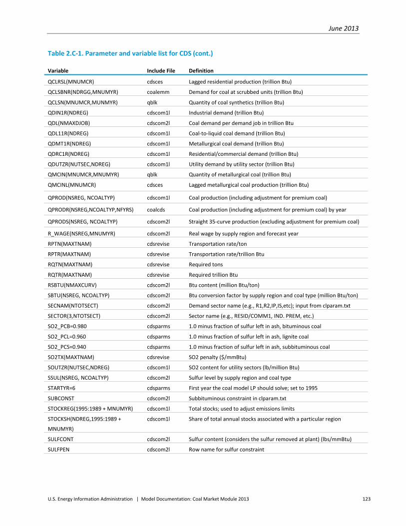
June 2013




QCLRSL(MNUMCR) cdsces Lagged residential production (trillion Btu)

QCLSBNR(NDRGG,MNUMYR) coalemm Demand for coal at scrubbed units (trillion Btu)

QCLSN(MNUMCR,MUNMYR) qblk Quantity of coal synthetics (trillion Btu)

QDIN1R(NDREG) cdscom1l Industrial demand (trillion Btu)

QDL(NMAXDJOB) cdscom2l Coal demand per demand job in trillion Btu

QDL11R(NDREG) cdscom1l Coal-to-liquid coal demand (trillion Btu)

QDMT1R(NDREG) cdscom1l Metallurgical coal demand (trillion Btu)

QDRC1R(NDREG) cdscom1l Residential/commercial demand (trillion Btu)

QDUTZR(NUTSEC,NDREG) cdscom1l Utility demand by utility sector (trillion Btu)

QMCIN(MNUMCR,MNUMYR) qblk Quantity of metallurgical coal (trillion Btu)

QMCINL(MNUMCR) cdsces Lagged metallurgical coal production (trillion Btu)

QPROD(NSREG, NCOALTYP) cdscom1l Coal production (including adjustment for premium coal)

QPRODR(NSREG,NCOALTYP,NFYRS) coalcds Coal production (including adjustment for premium coal) by year

QPRODS(NSREG, NCOALTYP) cdscom2l Straight 35-curve production (excluding adjustment for premium coal)

R_WAGE(NSREG,MNUMYR) cdscom2l Real wage by supply region and forecast year

RPTN(MAXTNAM) cdsrevise Transportation rate/ton

RPTR(MAXTNAM) cdsrevise Transportation rate/trillion Btu

RQTN(MAXTNAM) cdsrevise Required tons

RQTR(MAXTNAM) cdsrevise Required trillion Btu

RSBTU(NMAXCURV) cdscom2l Btu content (million Btu/ton)

SBTU(NSREG, NCOALTYP) cdscom2l Btu conversion factor by supply region and coal type (million Btu/ton)

SECNAM(NTOTSECT) cdscom2l Demand sector name (e.g., R1,R2,IP,IS,etc); input from clparam.txt

SECTOR(3,NTOTSECT) cdscom2l Sector name (e.g., RESID/COMM1, IND. PREM, etc.)

SO2_PCB=0.980 cdsparms 1.0 minus fraction of sulfur left in ash, bituminous coal

SO2_PCL=0.960 cdsparms 1.0 minus fraction of sulfur left in ash, lignite coal

SO2_PCS=0.940 cdsparms 1.0 minus fraction of sulfur left in ash, subbituminous coal

SO2TX(MAXTNAM) cdsrevise SO2 penalty ($/mmBtu)

SOUTZR(NUTSEC,NDREG) cdscom1l SO2 content for utility sectors (lb/million Btu)

SSUL(NSREG, NCOALTYP) cdscom2l Sulfur level by supply region and coal type

STARTYR=6 cdsparms First year the coal model LP should solve; set to 1995

SUBCONST cdscom2l Subbituminous constraint in clparam.txt

STOCKREG(1995:1989 + MNUMYR) cdscom1l Total stocks; used to adjust emissions limits

STOCKSH(NDREG,1995:1989 +

MNUMYR)

cdscom1l Share of total annual stocks associated with a particular region

SULFCONT cdscom2l Sulfur content (considers the sulfur removed at plant) (lbs/mmBtu)

SULFPEN cdscom2l Row name for sulfur constraint

June 2013




SUPNO(16,32) cdscom2l Supply curve number

SUPRGN(NSREG) cdscom2l Supply region

SURCHARGEI(4,NDREG,MNUMYR) cdscom1l Fuel surcharge for imports

SURCHART1(NSREG,NDREG,MNUMYR) cdscom1l Fuel surcharge for first tier electricity transportation rates

SURCHART2(NSREG,NDREG,MNUMYR) cdscom1l Fuel surcharge for second tier electricity transportation rates

SURFLAG cdscom1l If ‘1’, indicates that a surcharge is applicable to domestic shipments

SURFLAGI cdscom1l If ‘1’, indicates that a surcharge is applicable to imports

SUR_ADJ cdscom1l If SURFLAG equals ‘1’, indicates share of base year transportation rates

that already include a fuel surcharge

TIJL(NMAXPART,NMAXDJOB) cdscom2l Coal assigned by coal type (million tons)

TMPMBTU(MNUMYR) cdscom1l Average mercury emissions in tons of mercury per mmBtu

TONN(10,25,3,NFYRS) cdscom1l Import tonnage (million tons)

TOTALHOURS(NFYRS) cdscom2l Total labor hours by forecast year

TOTALWAGES(NFYRS) cdscom2l Total wages by forecast year

TOTLABPROD(MNUMYR) coalrep Total labor productivity in a given forecast year (tons/hour)

TOTPROD(NFYRS) cdscom2l Total production by forecast year

TRN_INDX(NUTSEC,NCOALTYP,NSREG,

NTOTDREG)

cdscom2l Index indicating whether transportation vector is required (0=Not

required; 1=Required)

TRUBND1(NSREG,NCOALTYP,NTOTDRE

G,NUTSEC)

cdscom1l Maximum volume of coal that may get the first tier transportation rate

by scrubbed and unscrubbed

TSPMBTU(MNUMYR) cdscom1l Average sulfur dioxide emissions in tons of sulfur dioxide per mmBtu

UCMERC(NUTSEC,MNUMYR) cdscom1l Uncontrolled mercury emissions

UCSO2(NUTSEC,MNUMYR) cdscom1l Uncontrolled sulfur dioxide emissions

UPEBYR uso2grp End banking year (year banked allowance cannot be used)

UPSLWFCTR uso2grp SO2 penalty price lower bound factor (currently 0.00)

UPSYEAR uso2grp Year to start creating SO2 penalty price bounds (currently 1999)

UPTPSO2(MNUMYR+1) uso2grp Target SO2 penalty price

USINTLDR=4 cdsparms International U.S. demand regions (UI,UE,UG, and UN)

USPLIT=6 cdsparms Utility coal types for reporting (old, new, scrubbed, and low-, medium-,

and high-sulfur)

UTCONS coalrep Utility coal consumption (trillion Btu)

UTPSO2 coalrep Utility potential SO2 emissions (million tons)

WAGEGROWTH(MNUMYR) coalrep Growth in wages from 2001

WAGEPHOUR(MNUMYR) coalrep Total wage per hour by year

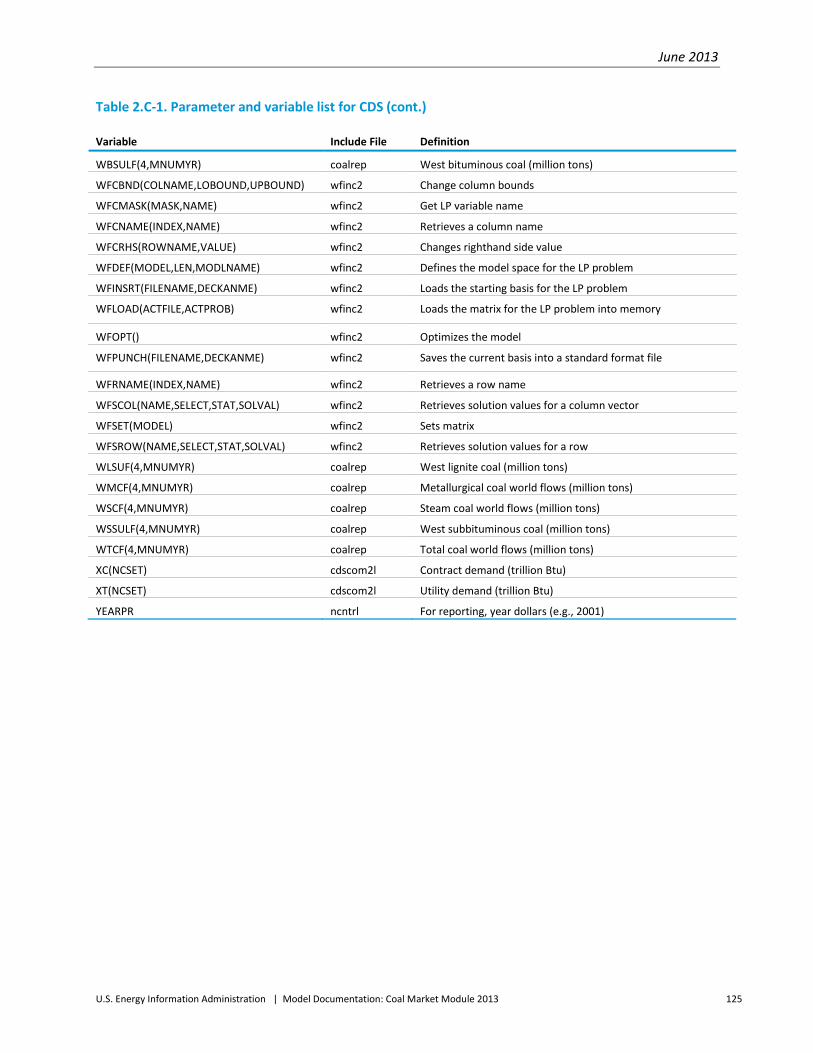
June 2013




WBSULF(4,MNUMYR) coalrep West bituminous coal (million tons)

WFCBND(COLNAME,LOBOUND,UPBOUND) wfinc2 Change column bounds

WFCMASK(MASK,NAME) wfinc2 Get LP variable name

WFCNAME(INDEX,NAME) wfinc2 Retrieves a column name

WFCRHS(ROWNAME,VALUE) wfinc2 Changes righthand side value

WFDEF(MODEL,LEN,MODLNAME) wfinc2 Defines the model space for the LP problem

WFINSRT(FILENAME,DECKANME) wfinc2 Loads the starting basis for the LP problem

WFLOAD(ACTFILE,ACTPROB) wfinc2 Loads the matrix for the LP problem into memory

WFOPT() wfinc2 Optimizes the model

WFPUNCH(FILENAME,DECKANME) wfinc2 Saves the current basis into a standard format file

WFRNAME(INDEX,NAME) wfinc2 Retrieves a row name

WFSCOL(NAME,SELECT,STAT,SOLVAL) wfinc2 Retrieves solution values for a column vector

WFSET(MODEL) wfinc2 Sets matrix

WFSROW(NAME,SELECT,STAT,SOLVAL) wfinc2 Retrieves solution values for a row

WLSUF(4,MNUMYR) coalrep West lignite coal (million tons)

WMCF(4,MNUMYR) coalrep Metallurgical coal world flows (million tons)

WSCF(4,MNUMYR) coalrep Steam coal world flows (million tons)

WSSULF(4,MNUMYR) coalrep West subbituminous coal (million tons)

WTCF(4,MNUMYR) coalrep Total coal world flows (million tons)

XC(NCSET) cdscom2l Contract demand (trillion Btu)

XT(NCSET) cdscom2l Utility demand (trillion Btu)

YEARPR ncntrl For reporting, year dollars (e.g., 2001)

June 2013


Output and composition of reports

Current output from the domestic component of the CDS falls into three categories:

The NEMS system currently generates five domestic coal reports in the NEMS table array (Tables 16 and the Supplement to the Annual Energy Outlook tables 109,110, 111, and 115).

• An output file (@.CLCDS) that currently contains five year-specific detailed reports. These reports are intended for use in model diagnosis, calibration and to provide detailed output for special studies. Only those currently operational are reviewed in this appendix. For diagnostic purposes, the reports in this file may be generated for each iteration of the CDS.

• A second file (@.CLDEBUG) contains output showing the performance of the CDS Fortran code and is used for diagnostic purposes.

NEMS Tables

Prices and quantities produced by the CDS occur throughout the NEMS tables. However, the bulk of domestic CDS output is reported in seven NEMS tables dedicated entirely to coal. These reports can be found using the interactive table viewer (http://www.eia.gov/oiaf/aeo/tablebrowser/). These reports are organized to show selected NEMS coal quantities and prices for each year in the forecast period., "Coal Supply, Disposition, and Prices" (http://www.eia.gov/oiaf/aeo/tablebrowser/#release=AEO2013&subject=7-AEO2013&table=15-AEO2013&region=0-0&cases=ref2013-d102312a) shows:

• Production east and west of the Mississippi River and for the Appalachian, Interior and Western regions, and the national total in millions of short tons

• Imports, exports, and net imports, plus total coal supply in millions of short tons • Sector consumption for the residential/commercial, industrial steam, industrial coking, and

electricity sectors plus total domestic consumption in millions of short tons • Annual discrepancy (including the annual stock change) • Average minemouth price in dollars per ton (the dollar year is provided) • Sectoral delivered prices in dollars per ton for the industrial steam, industrial coking, and

electricity sectors, and the weighted average for these three sectors • Average free-alongside-ship price for exports, i.e., the dollar-per-ton value of exports at

their point of departure from the United States

http://www.eia.gov/oiaf/aeo/tablebrowser/#release=AEO2013&subject=7-AEO2013&table=15-AEO2013&region=0-0&cases=ref2013-d102312a


June 2013


"Coal Production and Minemouth Prices By Region" (http://www.eia.gov/oiaf/aeo/tablebrowser/#release=AEO2013&subject=7-AEO2013&table=94-AEO2013&region=0-0&cases=ref2013-d102312a) provides annual summaries of national distribution aggregated supply regions, plus subtotals for five subregions: "Appalachia," "Interior," "Western," "East of the Mississippi River," and "West of the Mississippi River." In the lower half of the table, minemouth prices are shown in dollars per ton for the same regions and subtotals.

"Coal Production by Region and Type" (http://www.eia.gov/oiaf/aeo/tablebrowser/#release=AEO2013&subject=7-AEO2013&table=95-AEO2013&region=0-0&cases=ref2013-d102312a) lists production in millions of short tons per forecast year by supply region by coal rank and sulfur level.

"Coal Minemouth Prices by Region and Type" ( http://www.eia.gov/oiaf/aeo/tablebrowser/#release=AEO2013&subject=7-AEO2013&table=99-AEO2013&region=0-0&cases=ref2013-d102312a) lists minemouth prices for each forecast year by supply region by coal rank and sulfur level.

Additionally, three tables show international seaborne coal trade projections for coal by international supply regions to the Europe/Mediterranean region, Asia, and the Americas. They can be found at the following links: http://www.eia.gov/oiaf/aeo/tablebrowser/#release=AEO2013&subject=7-AEO2013&table=99-AEO2013&region=0-0&cases=ref2013-d102312a (for steam coal trade), http://www.eia.gov/oiaf/aeo/tablebrowser/#release=AEO2013&subject=7-AEO2013&table=97-AEO2013&region=0-0&cases=ref2013-d102312a (for metallurgical coal trade), and http://www.eia.gov/oiaf/aeo/tablebrowser/#release=AEO2013&subject=7-AEO2013&table=98-AEO2013&region=0-0&cases=ref2013-d102312a (for total coal trade).

National coal production, consumption, and exports are reported in quadrillion Btu in the “Total Energy Supply, Disposition, and Price Summary” (http://www.eia.gov/oiaf/aeo/tablebrowser/#release=AEO2013&subject=0-AEO2013&table=1-AEO2013&region=0-0&cases=ref2013-d102312a), as is the minemouth price of coal in dollars per ton.Annual energy consumption for the Residential, Commercial, Industrial (both industrial steam and coking consumption are shown) and the Electric Power sector in quadrillion Btu are shown in”Energy Consumption by Sector and Source” (http://www.eia.gov/oiaf/aeo/tablebrowser/#release=AEO2013&subject=0-AEO2013&table=2-AEO2013&region=1-0&cases=ref2013-d102312a). “Energy Prices by Sector and Source” (http://www.eia.gov/oiaf/aeo/tablebrowser/#release=AEO2013&subject=0-AEO2013&table=3-AEO2013&region=1-0&cases=ref2013-d102312a) gives delivered coal prices for these same sectors in dollars per million Btu. The table “Conversion Factors” (http://www.eia.gov/oiaf/aeo/tablebrowser/#release=AEO2013&subject=0-AEO2013&table=20-AEO2013&region=0-0&cases=ref2013-d102312a) shows Btu conversion rates for coal production (east and west of the Mississippi River, and the national average), and for coal consumed in the domestic NEMS sectors (Residential/Commercial, Industrial, Coking, and Electricity sectors).

Single Year Detailed Reports















June 2013


The first report that is output to the CDS file is the Census Division Report, which shows sectoral statistics by Census division and for the Nation. The statistics reported are production in millions of tons, demand in trillion Btu, and the sectoral average Btu conversion factor. The minemouth, transportation, and delivered prices are shown in dollars per ton, and the delivered price is also shown in dollars per million Btu. No prices are shown for imported coal since it is not priced in the model. The next report, the Detailed Demand and Price Report, describes each demand met by the model in the year described and shows each increment of supply that contributes to every demand in millions of tons. The demands are shown in millions of short tons and trillion Btu. This report also contains the adjusted minemouth price for each participant, the origin of the coal shipped, the type of coal shipped, and the associated transportation rate. Average prices and total quantities are provided for the major sectors in each demand region. This report is about 14 pages in length, depending on the year and scenario reported (usually one page per demand region).These reports are currently followed by a series of three single-page regional summary production reports. The first shows regional production and minemouth price (in millions of short tons and dollars per ton, respectively) by mine type. The second shows the same items by coal rank, while the third shows them by coal sulfur level.

These summary reports are followed by the Detailed Coal Production Report, showing the production, minemouth price, total energy content and Btu conversion factor for each coal supply source used in the reported year. This report is also formatted as a spreadsheet, with the coal types shown as rows and the supply regions as columns.

June 2013


Appendix 2.D. Data Quality and Estimation Development of the CDS transportation index

In AEO2013, coal transportation costs, both first- and second-tier rates, are modified over the forecast horizon by two regional (East and West) transportation indices. The indices, calculated econometrically, are measures of the change in average transportation rates, on a tonnage basis, that occurs between successive years for coal shipments. The methodology used to formulate these indices was first revised for AEO2009. In AEO2013, an East index is used for coal originating from eastern supply regions, while a West index is used for coal originating from western supply regions. The East index is a function of railroad productivity, the user cost of capital for railroad equipment, and the national average diesel fuel price. The user cost of capital for railroad equipment is calculated from the producer price index for railroad equipment, projected to remain flat in real terms, and accounts for the opportunity cost of money used to purchase equipment, depreciation occurring as a result of use of the equipment (assumed at 10 percent per year), less any capital gain associated with the worth of the equipment. The West index is a function of railroad productivity, gross capital expenditures for Class I railroads, and western share of national coal consumption. The indices are universally applied to all domestic coal transportation movements within the CMM. In the AEO2013 reference case, western coal transportation rates are 1 percent higher in 2040 and eastern rates are projected to be flat in 2040 compared to 2011.

Background

Transportation rates can be expected to change over time as market conditions change. Historically, the majority of transportation agreements involved contracts that extended over many years. Despite the length of these contracts, escalator clauses were typically employed allowing rates to change in accordance with changing market conditions. In addition, shorter contracts, which have become more prevalent, provide an opportunity for both parties involved to renegotiate their positions more frequently. The transportation indexing methodology used in AEO2013 is needed within the CDS to simulate the changes that may occur in real coal transportation rates over the forecast horizon.

Prior to the Annual Energy Outlook 1997 (AEO1997), transportation indexing factors were derived from index data published by the Association of American Railroads. Beginning in AEO1997 and extending through AEO2004, an indexing methodology based on the producer price index (PPI) for the transportation of coal via rail was used. The PPI for coal transportation tracks the national average change in prices received by railroads for the transportation of coal. A statistical regression model was fitted to the PPI for coal rail transportation. The independent variables used in the formulation were intended to account for the input costs that would affect transportation rates over time and in the AEO1997 formulation included: trend (as a proxy for productivity), the price of No. 2 distillate fuel to the industrial sector, the PPI for transportation equipment, and the national average wage rate. (For more information regarding this formulation, see "Forecasting Annual Energy Outlook Coal Transportation Rates" by Jim Watkins in Issues in Midterm Analysis and Forecasting 1997.) For AEO2004, the PPI for rail transportation equipment was substituted for the PPI for transportation

June 2013


equipment as one of the independent variables. The PPI for rail transportation equipment was also converted to the user cost of capital of transportation equipment for use in the regression. In addition, for AEO2004, the average rail wage replaced the national average wage rate in the econometric formulation.

For AEO2005, the methodology used to derive the transportation index was again revised. The principal goals of the development of a revised transportation escalator for AEO2005 were a statistically significant regression that included East and West regional differentiation and an improved representation of productivity. Although the factors that affect costs in the East and West are largely the same, there is evidence suggesting the weights of these factors on transportation costs differ for these two regions. For instance, western coal traffic tends to be associated with longer hauls than eastern traffic. Hence, the effect of distance on the change in average transportation cost for western traffic is assumed to be more influential. In addition to the incorporation of a regional component, an improved representation of productivity was also an objective. In previous formulations of the transportation index, time trend served as a proxy for productivity. Time trend is not amenable to the development of sensitivity cases in which productivity falls or increases; therefore an alternative was sought.

For AEO2009, the methodology for the transportation index was once again revised. This same basic methodology is used in AEO2013. A revision was required because the FERC 580 survey, the basis for the AEO2005 methodology, only includes a sample of coal shipments to electric utilities. As deregulation lowered the number of utilities nationwide, this sample size dropped even more. So, an update of the historical information for the dependent variable (transportation rate), distance, and contract information, all previously derived from the FERC Form 580, would not be representative of all coal shipments. The revised AEO2009 (and AEO2013) methodology combines the historical FERC Form 580 information through 1999 (supplemented with information from the Surface Transportation Board’s Carload Waybill Sample) with the average transportation rates inferred from the FERC Form 423, EIA 423 surveys, and EIA-7A surveys for the years 2000 through 2005 to approximate the dependent variable of the equation. The current methodology used in AEO2013 is based on data through 2006.

Theoretical approach

The general intent of the transportation index is to account for the variables that are correlated with or impact non-inflationary changes in average coal transportation rates over time. The approach taken to develop a revised formulation included a review of the factors contributing to historical changes in transportation rates, the development of a list of potential predictive variables, and the actual development of a regression model.

While coal is transported by rail, barge, truck, and conveyor, the most frequently used form of transportation for coal is rail. In 1980, 59 percent of coal was transported by rail alone. In 2011, rail carried 72 percent of all domestic coal shipments. Currently, all modes of coal transportation are aggregated within the CDS. In addition, limited data resources are available for the less dominant modes of coal transport. For these reasons, the regression is formulated with a railroad focus.

June 2013


The Staggers Act of 1980 partially deregulated the railroad industry, allowing greater flexibility in the prices charged to rail customers. Since 1980 and through the 1990s, competitive pressures between rail companies inspired productivity improvements both related to and independent of the consolidation of the rail industry and the reduction of redundancies in the rail network. As the rail industry consolidated, many jobs were eliminated and replaced with investments in capital equipment. Unit trains, as long as 110 railcars and dedicated to the servicing of a single destination, contributed to improvements in average train speed and fuel economy. Larger, more powerful locomotives and the use of lighter aluminum rail cars, rather than those made entirely of steel, have also had a beneficial impact on productivity. Bigger rail cars, capable of holding 100 tons each, longer train sets, and double tracking are also among the improvements cited by the rail industry.

The Clean Air Act Amendments of 1990 (CAAA90) imposed sulfur dioxide emissions limits on the electric power industry. As a result, more low-sulfur western coal was being used and shipped to locations much further away than previously thought practical. This coal, lower in thermal content than typical eastern bituminous coals, previously was regarded as too high in moisture content and too volatile to transport long distances. Also, transportation rates from western supply regions became increasingly competitive to help western coal penetrate eastern markets. Lower competitively priced transportation rates, coupled with low western minemouth prices and lower sulfur content, made many generators interested in at least trying western subbituminous coal. For AEO2013 for the West transportation index, an increasing share of western coal required to satisfy national coal demand is assumed to be negatively correlated with transportation rates.

The railroad industry is capital-intensive and requires investments in the purchase and servicing of equipment such as freight cars, land, inventory, and structures such as tracks. Without investments in capital structure, many productivity improvements would not have occurred in the historical period. For this reason, some representation of investment was deemed to be a necessity for the current formulation. For the East regression, the PPI for rail transportation equipment was transformed into a user cost of capital for rail equipment by accounting for the interest rate, depreciation, and any capital gain or loss associated with the investment. Unlike productivity, which is expected to push prices downward, with all other variables held constant, an increase in the user cost of capital tends to increase transportation rates. For the West, the same term did not prove significant. Instead, gross capital expenditures for Class I railroads was used as a proxy for western railroad investments.

While diesel fuel historically has represented a fairly small share, 9 percent,24 of railroad operating costs and fixed charges, recent years’ high fuel costs are assumed to have an increasing impact on overall transportation costs. The diesel fuel price is included as an explanatory variable for the eastern formulation for 2001 through 2006. Diesel fuel prices did not appear to be significant for the western formulation and do not have an effect on the formula for the east in the years prior to 2001.

24 Association of American Railroads, AAR Railroad Cost Indexes (September 2003), p. 4.

June 2013


For the dependent variable, calculated prices from the Coal Transportation Rate Database (CTRDB) were used to develop the index for the historical period from 1980 to 1999. These data were based on the FERC 580 Form in combination with supplemental data from the Surface Transportation Board’s Carload Waybill Sample. Multi-mode shipments were included with rail since rail travel is frequently a component of multi-mode shipments. For the time period 2000 through 2006 average transportation rates were inferred from the FERC Form 423 and EIA-423 surveys and the EIA Form 7A. The 423 surveys provide delivered price information for the electricity sector while minemouth prices are obtained from the EIA-7A survey. The difference between the delivered prices and minemouth price is assumed to be the transportation rate. The resulting data series was merged with the CTRDB data by rebasing both series to their respective 1999 values (indexed to 1.00).

The regression analysis relies on the following explanatory variables: productivity, user cost of capital of railroad equipment (east), investment dollars (west), diesel fuel price (east), and western share of national coal demand (west). These were chosen due to their ability to explain the historical time period, their availability, the ability to develop reasonable estimates of their future values for NEMS, and their ability to generate a statistically reasonable regression.

Equation specification

EAST INDEX = f(PRODUCTIVITY, USER COST OF CAPITAL OF RAILROAD EQUIPMENT, DIESEL FUEL PRICE)

and

WEST INDEX = f(PRODUCTIVITY, INVESTMENT DOLLARS, WESTERN SHARE OF NATIONAL COAL DEMAND)

Variables:

EAST and WEST INDEX, the dependent variables, are the values of the transportation price index in year t for coal originating East of the Mississippi River and West of the Mississippi River, respectively. For the historical data series (1980 through 1999), this value is calculated from the yearly average transportation rates (dollars per ton) calculated from the CTRDB for rail and multi-mode shipments of coal originating from eastern supply sources for the East index and from western supply sources for the West index. The CTRDB nominal dollars per ton is subsequently divided by the chain-weighted implicit gross domestic product (GDP) deflator to convert the rate to real 1987 dollars, and has a value of 1 in 1999 because it was rebased to 1999.

The CTRDB represents only a subset of the electric power industry. The CTRDB is mainly based on the FERC 580 Form, "Interrogatory on Fuel and Energy Purchase Practices," which collects information from jurisdictional utilities (investor-owned utilities that sell electric power at wholesale prices to other utilities) owning at least one power plant of 50 MW or more. The FERC 580 collects coal shipment information and transportation costs related to contract shipments between coal utilities and coal producers and brokers of one year or greater in duration on a biannual basis. This database is also supplemented with data from the Surface Transportation Board's Carload Waybill Sample.

June 2013


For 1998 through 2006, transportation rate data were imputed using the difference between the delivered price of coal to the electricity sector on the FERC and EIA-423 and the minemouth prices from the EIA-7A. This methodology was not used for earlier years due to the unavailability of data before 1998. For this series, data were rebased so that 1999 equals 1.00 and then merged with the CTRB data for the years 1999 through 2006.

PRODUCTIVITY is defined as billion ton-miles per employee per year for Class I railroads. This variable has not been converted to an index. The ton-miles and employee information is derived from data collected by the Association of American Railroads (AAR) and annual reports from the four largest major freight railroads and represents productivity for these railroads’ entire freight traffic, not just coal.

Ton-miles per employee is calculated by multiplying the total revenue tons by the average length of haul for all freight shipments divided by the number of railroad employees for Class I railroads. Class I railroads are defined by the Surface Transportation Board as those line haul freight railroads whose adjusted annual operating revenues for three consecutive years exceed 250 million dollars.25 The definition of Class I railroads has changed over time as the revenue criteria has changed and railroads enter and exit the railroad industry. Class I railroads generate the majority of the revenue and move the majority of the freight in the rail industry. In performing the calculation, East tons and average haul are calculated from shipments originating in the East while West tons and average haul are calculated from shipments originating in the West. In calculating the number of Eastern employees, the following railroad companies were included in the historical series: CSX Transportation, Norfolk Southern, Consolidated Rail, Illinois Central, and Florida East Coast Railway Company. In calculating the number of Western employees, the following railroad companies were included in the historical series: Union Pacific, Burlington Northern & Santa Fe, Southern Pacific, Atchison, Topeka & Santa Fe, Chicago & North Western, Grand Trunk Corporation, Soo Line Railroad, and Kansas City.

USER COST OF CAPITAL OF RAILROAD EQUIPMENT (UCC) is calculated from the producer price index (PPI) for railroad equipment. The PPI is obtained from the Bureau of Labor Statistics series WPS144. The user cost of capital is intended to capture the true cost of purchasing transportation equipment. The user cost of capital accounts for the opportunity cost of money used to purchase the equipment,

25 Surface Transportation Board, Statistics of Class I Freight Railroads 2003, website http://stb.dot.gov/stb/industry/econ_reports.html.

http://stb.dot.gov/stb/industry/econ_reports.html

June 2013


depreciation occurring as a result of use of the equipment (assumed at 10 percent), less any capital gain associated with the worth of the equipment. The formula to convert the PPI to a user cost of capital is the following:

UCCt = (rt + δ - (pt - pt-1)/pt-1) * pt

where

rt is a proxy for the real rate of interest, where rt = ((AA Utility Bond Ratet + greenhouse gas risk premium)/100) – [GDP Deflatort – GDP Deflatort-1)/GDP Deflatort-1]; δ is the rate of depreciation on railroad equipment, assumed to equal 10 percent per year;

and

pt is the PPI for railroad equipment, adjusted to constant 1987 dollars using the GDP deflator for year t.

The three terms represented in the annual user cost of railroad equipment are defined as follows:

rpt is the opportunity cost of having funds tied up in railroad equipment in year t;

δpt is the compensation to the railroad company for depreciation in year t; and

((pt - pt-1)/ pt-1)) pt is the capital gain on railroad equipment (in a period of declining capital prices, this term will take on a negative value, increasing the user cost of capital for year t).

INVESTMENT is calculated from the gross capital expenditures of Class I railroads in a given year, sourced from the U.S. Census Bureau Statistical Abstract. These gross capital expenditures include expenditures on equipment, roadway, and structures.

WESTERN SHARE OF NATIONAL TOTAL COAL PRODUCTION is the total proportion of coal produced that is supplied from west of the Mississippi River. This rising share since 1980 has been correlated with declining transportation rates through and including 2005 as the West sought to increase its market share. This variable is assumed to be correlated with changes in transportation rates in the projection period.

RHO: In conducting the regression for the East and West index, the Durbin-Watson statistic indicated autocorrelation was present. Autocorrelation indicates that some portion of the error term is capable of being forecasted but is not represented by the independent variables in the equation. A correction for autocorrelation, rho, was incorporated into the equations procedure in TSP 4.5 with the AR1 option for first-order correlation.

June 2013


A semi-log linear specification was used to develop the West econometric formula. Using ordinary least squares (OLS) regression and correcting for autocorrelation, the following equations were derived:

EAST INDEX = [EAST INDEXt-1rhoe + (AE * (1 - rhoe)) + (B1* productivityt ) - (B1*rhoe* productivityt -1) +

(B2* uccrequt) - (B2 * rhoe * uccrequt -1 ) + (B3* DUM05* diesel fuel pricet) - (B3*rhoe* DUM05*diesel fuel pricet -1) ]/EAST INDEXO

WEST INDEX = [WEST INDEXt-1rho * exp(AW * (1 - rhow)) + (B5*investt) - (B5*rhow* investt-1) +

(B4*productivityt) - (B4 * rhow *productivityt-1 ) + (B6*DUM*wshnatlt) - (B6*rhow*DUM*wshnatlt-1) ]/WEST INDEXO

where

AE = constant term B1 = the regression coefficient for productivity B2 = the regression coefficient for the user cost of capital B3 = the regression coefficient for the diesel fuel price DUM05 = 1 if year 2005, else 0 rhoe= correction for autocorrelation EAST INDEXO = the value of EAST INDEX in the base year of the forecast (2011) AW = constant term B5 = the regression coefficient for investment B4 = the regression coefficient for productivity B6 = the regression coefficient for the western share of national coal demand DUM = 1 for years < 2006, but 0 for 2006 rhow = correction for autocorrelation

WEST INDEXO = the value of WEST INDEX in the base year of the forecast (2011) uccrequ = user cost of capital for railroad equipment wshnatl = western share of national coal demand for 1981-2005 invest = Class I railroad investment dollar index

June 2013


Table 2.D-1. Statistical regression results

EAST INDEX WEST INDEX

Method of estimation: Ordinary Least Squares Ordinary Least Squares

Number of observations: 27 (years 1980-2006) 26 (years 1981-2006)

Mean of dependent variable: 1.29086 0.262376

Standard deviation of dep. var.: .216717 0.335155

Sum of squared residuals: .131569 0.045453

Variance of residuals: 0.598043-02 0.216443-02

Standard error of regression: 0.077333 0.0465223

R2: 0.892330 0.984019

Adjusted R2: 0.872753 0.980975

Rho: 0.361206 0.547600

Durbin-Watson: 1.77288 1.85383

Schwarz B.I.C.: -29.710825.3577 -37.9701

Log likelihood: 37.856133.5973 46.1153

EAST INDEX

Variable

Estimated

Coefficient Standard Error t-statistic P-value

Constant 1.59107 0..120371 13.2180 [0.000]

Productivity -0.124193 .013626 -9.11410 [0.000]

User cost of capital for rail

equipment

0.011394 0.486063-02 2.34421 [0.019]

Diesel fuel price 0.077039 0.010463-02 7.36320 [0.000]

Rho 0.361206 0.203607 1.77403 [0.076]

WEST INDEX

Variable

Estimated

Coefficient Standard Error t-statistic P-value

Constant 0.632603 0.132541 4.77287 [0.000]

Productivity -0.111765 0.010056 -11.1148 [0.000]

Western share of national coal demand for

years less than 2006

-0.264830 0.087420 -3.02939 [0.002]

Investment 0.434937 0.154393 2.81707 [0.005]

Rho 0.547600 0.232696 2.35329 [0.019]

June 2013


Table 2.D-2. Data sources for transportation variables

Variable Units Historical Data Forecasted Data

Transportation Rate No units (index) 1980-1999:Derived from U.S. Energy

Information Administration, Coal

Transportation Rate Database (CTRDB);

2000-2006: imputed from difference

between delivered prices on FERC/EIA Form

423 and minemouth prices from EIA-7A

Forecasted endogenously

from econometric

equation.

Productivity Billion Freight Ton-

Miles/Employee

Derived from data from the Association of

American Railroads and Class I Railroads’

Annual 10-K Reports

Projected to remain flat

from 2011 levels

User Cost of Capital for

Rail Equipment

No units (index) Derived from the PPI for rail equipment

from Bureau of Labor Statistics (Series

WPS144).

PPI for rail equipment is

assumed to change

proportionately with year-

over-year changes in

national coal ton-miles

(estimated by model). For

each forecast year, a

three-year rolling average

of the PPI is used.

Gross Capital

Expenditures (includes

equipment, roadway,

and structures) for Class I

railroads

Million Dollars U.S. Census Bureau, Census Bureau

Statistical Abstract, (Washington, DC,

various editions), web site

http://www.census.gov/compendia/statab/

Changes proportionately

with year-over-year

change in national coal

ton-miles (estimated by

model)

Western share of

national coal demand

Percentage U.S. Energy Information Administration,

Annual Energy Review 2007, (Washington,

DC, June 2007), Table 3.3, website

http://www.eia.doe.gov/emeu/aer/pdf/aer.pdf

Linked to model output

Diesel Price Dollars per million Btu U.S. Energy Information Administration,

Annual Energy Review 2007, (Washington,

DC, June 2007), Table 3.3, website

http://www.eia.doe.gov/emeu/aer/pdf/aer.pdf

The coefficient in changed

to zero in order to avoid

double-counting the

effects of the fuel

surcharge discussed

below.

June 2013


Table 2.D-3. Historical data used to calculate east index

Year

Productivity

(East ton-

miles/East

employees)

UCC Rail

Equip

Diesel Fuel

Price

(nominal

dollars per

mmBtu)

Transportation Rate

(1987 dollars,

1999=1.00)

GDP

Deflator

1980 1.75 12.63 5.90 1.43 0.74

1981 1.82 21.39 7.17 1.58 0.81

1982 1.82 25.11 6.79 1.58 0.86

1983 2.24 24.54 5.96 1.61 0.89

1984 2.48 24.53 5.93 1.62 0.92

1985 2.52 21.81 5.69 1.48 0.95

1986 2.63 20.35 3.45 1.49 0.97

1987 3.11 21.30 3.97 1.45 1.00

1988 3.40 18.26 3.61 1.47 1.03

1989 3.54 14.44 4.22 1.39 1.07

1990 3.94 16.62 5.23 1.37 1.11

1991 4.09 16.99 4.67 1.34 1.15

1992 4.32 18.13 4.46 1.20 1.18

1993 4.66 16.80 4.34 1.24 1.21

1994 5.07 15.75 3.99 1.12 1.23

1995 5.35 14.44 4.04 1.14 1.26

1996 5.68 16.89 4.91 1.14 1.28

1997 6.07 19.96 4.63 1.14 1.30

1998 6.20 17.08 3.56 1.05 1.32

1999 6.04 17.54 4.21 1.00 1.34

2000 6.59 17.54 6.74 0.99 1.37

2001 6.94 17.27 6.07 1.24 1.40

2002 7.47 16.48 5.49 1.15 1.42

2003 7.78 14.37 6.81 0.91 1.45

2004 8.52 10.14 8.96 0.96 1.50

2005 8.35 4.40 12.88 1.29 1.54

2006 8.34 10.96 15.11 1.51 1.59

June 2013


Table 2.D-4. Historical data used to calculate west index

Year

Productivity (West

ton-miles/West

employees)

Investment

(1987 dollars,

1981= 1.00)

Western Share of

National Coal

Demand

Transportation Rate

(1987 dollars,

1999=1.00) GDP Deflator

1981 2.50 1.00 0.24 1.89 0.81

1982 2.57 0.97 0.24 1.96 0.86

1983 2.98 0.93 0.24 1.96 0.89

1984 3.31 1.19 0.24 2.15 0.92

1985 3.32 1.15 0.29 2.04 0.95

1986 3.64 1.13 0.23 2.13 0.97

1987 4.41 1.12 0.24 1.94 1.00

1988 4.88 1.12 0.26 1.73 1.03

1989 5.18 1.11 0.26 1.65 1.07

1990 5.47 1.06 0.30 1.57 1.11

1991 5.78 1.06 0.32 1.34 1.15

1992 6.21 1.04 0.31 1.33 1.18

1993 6.54 1.04 0.36 1.25 1.21

1994 7.20 1.05 0.36 1.19 1.23

1995 8.03 1.07 0.39 1.17 1.26

1996 8.64 1.15 0.37 1.10 1.28

1997 8.58 1.18 0.36 1.09 1.30

1998 8.71 1.24 0.38 1.02 1.32

1999 9.43 1.30 0.42 1.00 1.34

2000 10.11 1.30 0.42 0.92 1.37

2001 10.72 1.31 0.43 0.87 1.40

2002 11.00 1.30 0.44 0.87 1.42

2003 11.49 1.39 0.45 0.83 1.45

2004 11.94 1.42 0.48 0.83 1.50

2005 11.71 1.53 0.51 0.89 1.54

2006 11.97 1.54 0.53 0.97 1.59

For the projection period, the explanatory values are assumed to have varying impacts on the calculation of the indices. For both the East and West indices, investment is assumed to occur in response to changes in demand. This is measured by the change in ton-miles, as calculated by the model. If national ton-miles increase, the terms representing investment (for both the East and the West) are assumed to increase. Likewise, if ton-miles decrease, investment may decline. This assumption is derived partly from the assertion by railroads that they will be hesitant to make investments in capacity unless the demand is already present. Industry documents indicate that capital programs are correlated with the revenue received. Changes in ton-miles are naturally correlated with changes in revenue. In addition, other analysis has concluded that transportation investment is more sensitive to business cycles than other businesses. An increase in ton-miles necessitates investment to

June 2013


expand capacity and alleviate congestion, and a decline in ton-miles will similarly discourage investments.

Historically, cost savings derived from improvements in productivity have been accompanied by declining transportation rates. For both the East and the West, any related financial savings due to productivity improvements through 2040 are assumed to be retained by the railroads and are not passed on to shippers in the form of lower transportation rates. For that reason, productivity is held flat for the projection period for both regions. For the East, for the projection period, diesel fuel is removed from the equation in order to avoid double-counting the influence of diesel fuel costs with the impact of the fuel surcharge program.

Fuel Surcharge

Major coal rail carriers have implemented fuel surcharge programs in which higher transportation fuel costs have been passed on to shippers. While the programs vary in their design, the Surface Transportation Board (STB), the regulatory body with limited authority to oversee rate disputes, has recommended that the railroads agree to develop some consistencies among their disparate programs and has likewise recommended closely linking the charges to actual fuel use. The STB has cited the use of a mileage-based program as one means to more closely estimate actual fuel expenses.

A fuel surcharge program was incorporated into the coal transportation rates for the first time in AEO2007 and was based on BNSF Railway Company’s mileage-based program for all regions. For AEO2013, the methodology is based on BNSF Railway Company’s mileage-based program for western coal sources and for the East, the methodology is based on CSX Transportation’s mileage-based program. The surcharge becomes effective when the projected nominal distillate price to the transportation sector exceeds $1.25 per gallon for the West and $2.00 per gallon for the East. For the West, for every $0.06 per gallon increase above $1.25, a $0.01 per carload mile is charged, and for the East, every $0.04 per gallon increase above $2.00, a $.01 per gallon fee is assessed. The number of tons per carload and the number of miles vary with each supply and demand region combination and are a pre-determined model input. The final calculated surcharge (in constant dollars per ton) is added to the escalator-adjusted transportation rate.

For AEO2013, it was assumed that the base year (2011) transportation rates already included an assessed fuel surcharge. For AEO2013, the model calculates the fuel surcharges for 2011 and subtracts it from the corresponding base year transportation rate. These modified, lower, base-year transportation rates are used in subsequent forecast years and the fuel surcharges and transportation escalators for a specific forecast year are applied to these lower rates.

CDS Data Sources

EIA maintains a number of annual surveys of coal production and distribution. The agency also has access to several data surveys collected for the Federal Energy Regulatory Commission (FERC) that report the fuel purchase and delivery practices of the nation's electricity sector. Other information comes from Census Bureau forms reporting coal imports and exports. Data from the Association of

June 2013


American Railroads, the Surface Transportation Board, the Mine Safety and Health Administration, and State agency reports of mining activity supplement these sources.

• Form EIA-3, "Quarterly Coal Consumption and Quality Report, Manufacturing and Transformation/Processing Coal Plants and Commercial and Institutional Users," surveys heat, sulfur and ash content of coal receipts delivered to industrial steam, commercial, and institutional coal consumers by consumption location and state of origin.

• Form EIA-5, “Quarterly Coal Consumption and Quality Report, Coke Plants,” surveys volatility, sulfur and ash content of coal receipts delivered to coke plants by consumption location and state of origin.

• Form EIA-7A,"Coal Production and Preparation Report," covers coal producers and coal preparation plants and reports production, minemouth prices, coal seams mined, labor productivity, employment, stocks, and recoverable reserves at mines.

• Form EIA-423, “Monthly Cost and Quality of Fuels for Electric Plants Report,” covers electric non-utility plants with capacity of 50 MW or more and reports delivered cost, receipts, ash, Btu, sulfur ("As Received" basis), and sources. Beginning for 2008 data, Form EIA-923 replaces the EIA-423.

• FERC Form 423, "Monthly Report of Cost and Quality of Fuels for Electric Plants," covers electric utility plants with capacity of 50 MW or more and reports delivered cost, receipts, ash, Btu, sulfur ("As Received" basis), and sources. Beginning for 2008 data, Form EIA-923 replaces the EIA-423.

• Form EIA-923, “Power Plant Operations Report,” collects information from regulated and unregulated electric power plants in the United States. Data collected include electric power generation, energy source consumption, end of reporting period fossil fuel stocks, as well as the quality and cost of fossil fuel receipts.

• FERC Form 580, "Interrogatory on Fuel and Energy Purchase Practices", was a biennial survey of investor-owned utilities selling electricity in interstate markets and having capacity over 50 MW; coverage of contractual base tonnage, tonnage shipped, ash, Btu, sulfur and moisture ("As Received" basis), minemouth price, freight charges, coal source and destination, shipping modes, transshipments (if any), and distances.

• Form EM 545 from the U.S. Census Bureau records coal exports by rank, value and tonnage from each port district. The U.S. Census Bureau’s Form IM 145 reports imports by rank, value, tonnage, and port district.

• The Carload Waybill Sample, administered by the Surface Transportation Board, contains confidential information on a sample of waybills from those railroads that terminate at least 4,500 cars per year. The data collected includes origin, destination, tons, commodity type, revenue, and distance information. This information has been used to supplement EIA’s CTRDB database.

June 2013


Data gaps

The resources that are available to support the NEMS CPS and CDS include a series of databases derived from a variety of surveys that are valuable for their national scope and Census-like coverage. However, as shown in Table 2.D-5, no data from mines are routinely collected on the quality of coal produced at the mine or the minemouth price for coals of different quality levels. The EIA-923 has replaced the FERC Form 423 and the EIA-423 and now asks for mine origin information in addition to coal quality information. By doing this, in some instances, it is possible to infer some coal quality information for particular mines when the respondents have specific knowledge of their coal supplier. The EIA-923 together with the forms EIA-3 and EIA-5 (which provide state origin information) provide some coal quality data that assists in assigning coal quality information to coal supply regions.

While EIA publishes data identifying the tonnage of exported coal mined in each State and the Department of Commerce collects data on the tonnage exported (by port district), there are no available data to identify the tonnage from each mining State that is exported at each port of exit. Coals consumed by surveyed sectors (electricity, industrial, commercial/institutional and coking coal) are known to differ in quality from coals delivered to sectors currently unsurveyed (the residential, export metallurgical and export steam sectors). The EIA-7A requests information about export quantities. Where the coal quality characteristics of the mine can be inferred from information gathered on the EIA-923, some coal quality characteristics for exports can be likewise deduced. Consumption in the unsurveyed sectors currently accounts for a small percentage of production.

The difference between delivered costs as shown on the EIA-923, EIA-3, EIA-5, and EM 545 and minemouth costs as shown on Form EIA-7A in the most recent available historical year is used to estimate transportation rates. (Although commodity cost and delivered cost are available on the EIA-923, transportation rates are not currently calculated from the EIA-923 alone due to insufficient or incomplete information from the respondents.) The use of this method allows estimation of different rates from each supply curve to each sector in each demand region, but—even if data for more remote historical years were used—can do little to provide transportation rates for routes that have not been used. More than half the routes indicated by the CDS supply and demand region classification structures have not been used for coal transport in significant quantities in recent years. In the version of the CDS documented here, rates for these routes have been synthesized using available data on tariff rates and analytical judgment, while others that are unlikely to be used are given dummy values that prevent their use.

The general availability of coal-related data that were used to build and calibrate the CDS for the Annual Energy Outlook 2013 is summarized in Table 2.D-5.

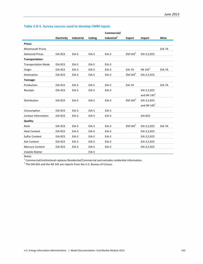
June 2013


Table 2.D-5. Survey sources used to develop CMM inputs

Electricity Industrial Coking

Commercial/

Industrial1 Export Import Mine

Prices:

Minemouth Prices EIA-7A

Delivered Prices EIA-923 EIA-3 EIA-5 EIA-3 EM 5452 EIA 3,5,923

Transportation:

Transportation Mode EIA-923 EIA-3 EIA-5 EIA-3

Origin EIA-923 EIA-3 EIA-5 EIA-3 EIA-7A IM 1452 EIA-7A

Destination EIA-923 EIA-3 EIA-5 EIA-3 EM 5452 EIA 3,5,923

Tonnage:

Production EIA-923 EIA-3 EIA-5 EIA-3 EIA-7A EIA-7A

Receipts EIA-923 EIA-3 EIA-5 EIA-3 EIA 3,5,923

and IM 1452

Distribution EIA-923 EIA-3 EIA-5 EIA-3 EM 5452 EIA 3,5,923

and IM 1452

Consumption EIA-923 EIA-3 EIA-5 EIA-3

Contact Information EIA-923 EIA-3 EIA-5 EIA-3 EIA-923

Quality:

Rank EIA-923 EIA-3 EIA-5 EIA-3 EM 5452 EIA 3,5,923 EIA-7A

Heat Content EIA-923 EIA-3 EIA-5 EIA-3 EIA 3,5,923

Sulfur Content EIA-923 EIA-3 EIA-5 EIA-3 EIA 3,5,923

Ash Content EIA-923 EIA-3 EIA-5 EIA-3 EIA 3,5,923

Mercury Content EIA-923 EIA-3 EIA-5 EIA-3 EIA 3,5,923

Volatile Matter EIA-5 Notes: 1 Commercial/institutional replaces Residential/Commercial and excludes residential information. 2 The EM 645 and the IM 145 are reports from the U.S. Bureau of Census.

June 2013


Appendix 2.E. Bibliography Abbey, David S. and Charles D. Kolstad, "The Structure of International Steam Coal Markets," Natural Resources Journal, 23 (1983), pp. 859-891.

Armington, P.S., A Theory of Demand for Products Distinguished by Place of Production, International Monetary Fund Staff Paper, 16 (1) (March 1969).

Averitt, Paul, Coal Resources of the United States, January 1, 1974, Bulletin 1412, U.S. Geological Survey (Washington, DC, 1975).

Bronzini, Michael S., "Evolution of a Multimodal Freight Transportation Network Model," Proceedings - Twenty First Annual Meeting, Transportation Research Forum, Volume XXI, Number 1 (Philadelphia, PA, 1980), pp. 475-485.

Bronzini, Michael S., "Network Routing and Costing Systems for Coal Transportation," Proceedings of Coal Transportation and Costing Seminar, October 15, 1984, prepared for the Electric Power Research Institute and the U.S. Department of Energy, (Kansas City, MO: the Argonne National Laboratory, July 1985).

Bureau of the Census, U.S. Department of Commerce, Historical Statistics of the United States, Colonial Times to 1970, Part I (Washington, DC, 1975).

Coal Age, vol.87, No.5, (May 1982).

Data Resources, Inc., Coal Service Documentation, (Lexington, MA, March, 1981).

Day, R.H. and W.K. Tabb, 1972, A Dynamic Microeconomic Model of The U.S. Coal Mining Industry, SSRI Research Paper (Madison, WI: University of Wisconsin, 1972).

Dunbar, Frederick C. and Joyce S. Mehring, "Coal Rail Prices During Deregulation: A Hedonic Price Analysis," Logistics and Transportation Review, vol. 26, No.1, 1990.

Friesz, T.L., J. Gottfried, R.E. Brooks, A.J. Zielen, R. Tobin and S.A. Meleski, The Northeast Regional Environmental Impact Study: Theory, Validation and Application of A Freight Network Equilibrium Model, ANL/ES - 120, Division of Environmental Impact Studies, Argonne National Laboratory, prepared for the Economic Regulatory Administration, U.S. Department of Energy, (Washington, D.C., 1982).

Gayver, Donald P. and Gerald I. Thompson, Programming and Probability Models in Operations Research (New York: Wadsworth, 1973).

Gordon, Richard, Coal Industry Problems, Final Report, EA 1746, Project 1009-4, prepared by the Pennsylvania State University for the Electric Power Research Institute (Palo Alto, CA, June 1979), pp. 2-43, 2-44.

June 2013


Grennes, T. J., P.R. Johnson, and M. Thursby, The Economics of World Grain Trade (New York: Praeger, 1978).

Groncki, P.J. and W. Marcuse, "The Brookhaven Integrated Energy/Economy Modeling System and Its Use in Conservation Policy Analysis," Energy Modeling Studies and Conservation, ECE, ed., prepared for the United Nations, (New York: Pergamon Press, 1980), pp. 535-556.

Henderson, James M., The Efficiency of The Coal Industry, An Application of Linear Programming (Cambridge, MA: Harvard University Press, 1958).

Hudson, E.A. and D.W. Jorgenson, "U.S. Energy Policy and Economic Growth, 1975-2000," Bell Journal of Economics and Management Science, Vol.5, pp. 461-514.

ICF, Inc., The National Coal Model: Description and Documentation, Final Report (Washington, DC, October 1976).

ICF Resources, Inc., Documentation of the ICF Coal and Electric Utilities Model: Coal Transportation Network used in the 1987 EPA Interim Base Case, The U.S. Environmental Protection Agency (Washington, DC, September 1989).

Illinois State Geological Survey and the U.S. Bureau of Mines, U.S. Department of the Interior Engineering Study of Structural Geologic Features of The Herrin (No. 6) Coal and Associated Rock in Illinois, Volume 2, Detailed Report, NTIS PB-219462 (Washington, DC, June 1979).

Kolstad, Charles D., and David S. Abbey, "The Effect of Market Conduct on International Steam Coal Trade," European Economic Review, 24 (1984), pp. 39-59.

Kolstad, Charles D., David S. Abbey and Robert L. Bivins, Modeling International Steam-Coal Trade, LA-9661-MS, UC-98F (Los Alamos, NM: Los Alamos National Laboratory, January 1983).

Kolstad, Charles D. and Frank A. Wolak, Jr., "Competition in Interregional Taxation: The Case of Western Coal," Journal of Political Economy, vol. 91, No.3, (1983), pp. 443-460.

Labys, W.C. and Yang, C.W., "A Quadratic Programming Model of The Appalachian Steam Coal Market," Energy Economics, Vol.2., (1980), pp. 86-95.

LeBlanc, L.J., E.K. Morlok and W.P. Pierskalla, "An Efficient Approach to Solving the Network Equilibrium Traffic Assignment Problem," Transportation Research, Volume 9, pp. 309-318.

Leonard, Joseph W., W.F. Lawrence, and W.A. McCurdy, "Coal Characteristics and Utilization," Chapter 6 in J.W. Leonard, ed., Coal Preparation (New York: the American Institute of Mining, Metallurgical, and Petroleum Engineers, Inc., 1979).

Libbin, J.J. and X.X. Boehle, "Programming Model of East-West Coal Shipments," American Journal of Agricultural Economics, vol.27, 1977.

Locklin, D. Philip, Economics of Transportation (Homewood, IL: Richard D. Irwin, Inc. 1972).

June 2013


Murphy, F.H., The Structure and Solution of The Project Independence Evaluation System, prepared for the U.S. Energy Information Administration (Washington, DC, 1980).

Murphy, F.H., R.C. Sanders, S.H. Shaw and R.L. Thrasher, "Modeling Natural Gas Regulatory Proposals Using the Project Independence Evaluation System," Operations Research, vol. 29, pp. 876-902.

Newcombe, Richard T., "Mineral Industry Demands and General Market Equilibrium," Chapter 2.7, Economics of The Mineral Industries, 3rd ed. (New York: American Institute of Mining, Metallurgical and Petroleum Engineers, Inc, 1976).

Pennsylvania State University, "Zimmermann Coal Model," Economic Analysis of Coal Supply: An Assessment of Existing Studies, Volume 3, Final Report, EPRI EA-496, Project 335-3, prepared for the Electric Power Research Institute (Palo Alto, CA, June 1979).

Resource Dynamics Corporation, Coal Market Decision-Making: Description and Modeling Implications, Final Report to the Maxima Corporation for the Energy Information Administration (McLean, VA, June 1984).

Takayama, T., and G. Judge, Spatial and Temporal Price and Allocation Models (Amsterdam: North-Holland, 1971).

U.S. Energy Information Administration, Annual Coal Report 2011, DOE/EIA-0584(2011) (Washington, DC, November 2012), and previous issues.

U.S. Energy Information Administration, Coal Data: A Reference, DOE/EIA-0064(87) (Washington, DC, May 17, 1989).

U.S. Energy Information Administration, Coal Industry Annual, DOE/EIA-0584 (various years).

U.S. Energy Information Administration, Office of Electricity, Coal, Nuclear and Renewables Analysis, Coal Supply and Transportation Model (CSTM) Model Documentation, DOE/EIA-MO48 (Washington, DC, November 1991).

U.S. Energy Information Administration, Office of Coal, Nuclear, Electric and Alternate Fuels, Coal Supply and Transportation Model, Executive Summary, DOE/EIA-0401 (EXEC) (Washington, DC, August 1983).

U.S. Energy Information Administration, Coal Supply and Transportation Model: Model Description and Data Documentation, DOE/EIA-0401, (Washington, DC, August 1983).

U.S. Energy Information Administration, Office of Electricity, Coal, Nuclear and Renewables Analysis, "Development Plan for the National Energy Modeling System" (Washington, DC, draft of February 10, 1992).

U.S. Energy Information Administration, Documentation of the Integrating Module of the Intermediate Future Forecasting System, DOE/EIA-MO23(91) (Washington, DC, May 1991).

June 2013


U.S. Energy Information Administration, Documentation of the Project Independence Evaluation System (Washington, DC, 1979).

U.S. Energy Information Administration, U.S. Coal Reserves: A Review and Update, DOE/EIA-0529(95) (Washington, DC, August 1996).

U.S. Energy Information Administration, Mathematical Structure and Computer Implementation of the National Coal Model, DOE/EI/10128-2 (Washington, DC, January 1982).

U.S. Energy Information Administration, National Coal Model (NCM), Users Manual (Washington, DC, January 1982).

U.S. Energy Information Administration, Quarterly Coal Report, October-December 2011, DOE/EIA-0121 (2011/04Q) (Washington, DC, April 2012).

U.S. Energy Information Administration, Trends in Contract Coal Transportation, 1979-1987, DOE/EIA-0549 (Washington, DC, September, 1991).

U.S. General Accounting Office, Railroad Regulation, Economic and Financial Impacts of the Staggers Rail Act of 1980, GAO/RCED-90-80 (Washington, DC, May 1990).

United States Senate, Committee on Energy and Natural Resources, Committee on Commerce, Science, and Transportation, National Energy Transportation, Volume 1, Current System and Movements, Committee Print Publication No. 95-15 (Washington, DC, May 1977).

Valkovic, Vlado, Trace Elements in Coal, 2 vols. (Boca Raton, FL: CRC Press, 1983).

Vyas, A.D., "Overview of Coal Movement and Review of Transportation Methodologies," Proceedings of Coal Transportation Costing and Modeling Seminar, October 15, 1984 (Kansas City, MO: Argonne National Laboratory, July 1985), p. 7.

Wagner, Harvey M., "Network Models," Chapter 6 in Principles of Management Science with Applications to Executive Decisions (Englewood Cliffs, NJ: Prentice-Hall, Inc., 1970).

Watkins, Jim, "Forecasting Annual Energy Outlook Coal Transportation Rates," Issues in Midterm Analysis and Forecasting 1997, DOE/EIA-0607(97) (Washington, DC, July, 1997).

Wolak, Frank A. and Charles D. Kolstad, "Measuring Relative Market Power in The Western U.S. Coal Market Using Shapley Values," Resources and Energy, 10 (1988).

Zimmermann, M.B., "Estimating a Policy Model of U.S. Coal Supply," Advances in the Economics of Energy and Resources, vol. 2. (New York: JAI Press, 1979), pp. 59-92

Zimmermann, M.B., "Modeling Depletion in a Mineral Industry: The Case of Coal," Bell Journal of Economics, vol.8, No. 4 (Spring, 1977), pp. 41-65.

June 2013


Appendix 2.F. Coal Distribution Submodule Program Availability The source code for the CDS program is available from the program office:

Office of Electricity, Coal, Nuclear and Renewables Analysis EI-34 U.S. Energy Information Administration U.S. Department of Energy 1000 Independence Avenue S.W. Washington, DC 20585 Telephone: (202) 586-2415

June 2013


3. Coal Distribution Submodule — International Component

Introduction The purpose of Section 3 of the Coal Market Module documentation is to define the objectives and basic approach used to forecast international coal trade in the Coal Distribution Submodule (CDS), and to provide information on the model formulation and application. It is intended as a reference document for model analysts, users, and the public. The report conforms to requirements specified in Public Law 93-275, Section 57(B)(1) (as amended by Public Law 94-385, Section 57.b.2).

Model summary The international component of the CDS projects coal trade flows from 17 coal-exporting regions (5 of which are in the United States) to 20 importing regions (four of which are in the United States) for three coal types—coking, low-sulfur bituminous, and subbituminous. The model consists of exports, imports, trade, and transportation components. The major coal exporting countries represented include: the United States, Australia, South Africa, Canada, Indonesia, China, Colombia, Venezuela, Poland, the countries of the Former Soviet Union, and Vietnam. Beginning with AEO2006, the structure of the international component of the CDS has been updated to endogenously model U.S. imports. The U.S. import algorithm is integrated with the domestic component of the CDS.

Model archival citation and model contact The version of the CDS documented in this report is that archived for the forecasts presented in the Annual Energy Outlook 2013.

Name: Coal Distribution Submodule-International Component Abbreviation: CDS Archive Package: NEMS13(Available from the U.S. Energy Information Administration, Office of Electricity, Coal, Nuclear and Renewables Analysis) Model Contact: Diane Kearney, Department of Energy, EI-34, Washington DC 20585 (202) 586-2415 or ([email protected])

Organization This section of the report describes the modeling approach used in the International Component of the CDS used to project international coal trade. Subsequent sections of this report describe the following:

• The model objective, input and output, and relationship to other models • The theoretical approachand assumptions • The model structure, including key computations and equations

An inventory of model inputs and outputs, detailed mathematical specifications, bibliography, and model abstract are included in the Appendices.

June 2013


Model Purpose and Scope

Model objectives The objective of the international component of the CDS is to provide annual forecasts of world coal trade flows through 2040.

Coal exports in the international area of the CDS are modeled using three coal types: premium bituminous, low-sulfur bituminous, and subbituminous coals (Table 3.1). These coal types represent unique combinations of heat and sulfur content. There are 17 geographic export regions (Table 3.2) including five U.S. export regions, two Canadian export regions, and 10 additional major coal exporting countries. The five U.S. coal export regions in the CMM (Figure 3.2) include the Northern Interior, the East Coast, the Gulf Coast, the Southwest and West, and the Non-Contiguous U.S. These U.S. regions represent aggregations of ports-of-exit through which exported coal passes on its way from domestic export regions to foreign consumers. For instance, the Northern Interior includes 12 ports of exit including locations ranging from Boston, Massachusetts to Great Falls, Montana. The Non-Contiguous U.S. region is only represented by two ports of exit, Anchorage and Seward, Alaska. These domestic port districts are identified in Table 3.2.

The coking and steam sectors define the international coal import sectors. The CMM coal types available to satisfy imports for the two international coal sectors are listed in Table 3.1. There are 20 coal import regions represented in the CMM (Table 3.3). The coal import regions for the United States are the same as the coal export regions except that the U.S. Southwest and West is excluded. Canada is split into two coal import regions, Eastern and Interior. The remaining 14 coal import regions are represented as either individual countries or groups of two or more countries.

The U.S. share of world coal markets is defined as a linear optimization problem and is solved simultaneously with the domestic coal forecast.

Four key user-specified inputs are required. They include coal import requirements, coal export curves, transportation costs, and constraints (Figure 3.1). The primary outputs are annual world coal trade flows.

Relationship to other modules The model generates regional forecasts for U.S. coal exports. These international U.S. export requirements are input to the domestic portion of the CDS so that sufficient production is allocated to U.S. exports. The CDS also projects U.S. imports required to satisfy coal demand in the United States established by the industrial and electricity models.

June 2013


Table 3.1. CDS international coal export types and demand sectors

Coal Export Type

Heat Content (million

Btu per short ton)

Sulfur Content

(Pounds sulfur per

million Btu)

Corresponding NEMS

CPS/CDS Coal Types Demand Sector

Premium >=25 <1.67 MDP, CDP Coking or Steam

Low-Sulfur Bituminous >=20 but < 25 <1.67 CDB, CSB, MDB, MSB Steam

Subbituminous <=15 but < 20 <0.60 CSS Steam

Figure 3. 1. International component inputs/outputs

June 2013


Figure 3.2. U.S. export and import regions used in the CDS

June 2013


Table 3.2. CDS coal export regions

Export Regions Domestic Port Districts

1 U.S. Northern Interior (I) Boston, MA

Portland, ME

St. Albans, VT

Buffalo, NY

Ogdensburg, NY

New York, NY

Philadelphia, PA

Detroit, MI

Cleveland, OH

Duluth, MN

Pembina, ND

Great Falls, MT

2 U.S. East Coast (E) Baltimore, MD

Norfolk, VA

Charleston, SC

Savannah, GA

Miami, FL

San Juan, PR

US Virgin Islands

Tampa, FL

3 U.S. Gulf Coast (G) Mobile, AL

New Orleans, LA

Houston-Galveston, TX

Laredo, TX

El Paso, TX

4 U.S. Southwest and West (W) Nogales, AZ

San Diego, CA

Los Angeles, CA

San Francisco, CA

Stockton, CA

Richmond, CA

Portland, OR

Seattle, WA

5 U.S. Non-Contiguous (A) Anchorage, AK

Seward, AK

6 Australia NA

7 Canada, Western NA

8 Canada, Interior NA

June 2013


Table 3.2. CDS coal export regions (cont.)

Export Regions Domestic Port Districts

9 South Africa NA

10 Poland NA

11 Eurasia (exports to Europe) NA

12 Eurasia (exports to Asia) NA

13 China NA

14 Colombia NA

15 Indonesia NA

16 Venezuela NA

17 Vietnam NA

Table 3.3. CDS coal import regions

Import Regions Countries

1 U.S. East Coast (E) NA

2 U.S. Gulf Coast (G) NA

3 U.S. Northern Interior (I) NA

4 U.S. Non-Contiguous (N) NA

5 Canada, Eastern NA

6 Canada, Interior NA

7 Scandinavia Denmark

Finland

Norway

Sweden

8 United Kingdom/Ireland NA

9 Germany/Austria NA

10 Other NW Europe Belgium

France

Luxembourg

Netherlands

11 Iberia Portugal

Spain

12 Italy NA

13 Med./E.Europe Algeria

Bulgaria

Croatia

Egypt

Greece

Israel

June 2013


Table 3.3. CDS coal import regions (cont.)

Import Regions Countries

Malta

Morocco

Romania

Tunisia

Turkey

14 Mexico NA

15 South America Argentina

Brazil

Chile

Peru

Puerto Rico

16 Japan NA

17 East Asia North Korea

South Korea

Taiwan

18 China/Hong Kong NA

19 ASEAN Malaysia

Philippines

Thailand

20 Indian sub/S. Asia Bangladesh

India

Iran

Pakistan

Sri Lanka

June 2013


Model rationale

Theoretical approach The core of the international component of the CDS is a linear programming optimization model. This LP model finds the pattern of coal production and trade flows that minimizes the production and transportation costs of meeting a set of regional net import requirements. The basic underlying assumption regarding the modeling of international coal trade in the CDS is that the international coal market is essentially a perfectly competitive market. The key conditions of a perfect market are that there are no real significant barriers to entry and exit on the export side, there are a large number of buyers and sellers, and no single buyer or seller controls enough of the market so as to be able to exert pricing power.

While a perfectly competitive market is the basic underlying assumption used for modeling international coal trade in the CMM, the model solution is subject to a number of key constraints:

• Export capacity of export regions. • Maximum share that any importing region can take from one exporting region. Coal buyers

(importing regions) will tend to spread their purchases among several suppliers in order to reduce the impact of supply disruption, even though this will add to their purchase costs.

• Maximum share that any exporting region will sell to one importing region. Coal producers (exporting regions) will choose not to rely on any one buyer, and will diversify their sales.

• Sulfur dioxide emission limits for U.S. imports. U.S. coal imports are subject to SO2 emission regulations as set forth under CAAA90 and Clean Air Interstate Rule. This is modeled by intersecting emissions from thermal imports in the electricity sector with the sulfur dioxide emissions constraint in the domestic component of the CDS.

• Mercury emission limits for U.S. coal imports. In scenarios where mercury emissions are restricted, imports are subject to the same limits as U.S. coal. When relevant, this is modeled by intersecting emissions from thermal imports in the electricity sector with the mercury row constraint in the domestic component of the CDS. For AEO2013, imports are subject to the Mercury Air Toxics Standard.

• Minimum (“contract”) flows for U.S. imports. These minimum flows are based on coal receipts data for existing U.S. power plants collected on EIA-923, “Power Plant Operations Report.”

Model structure The international component of the CDS is specified as part of the overall CDS Linear Program (LP). The LP satisfies import requirements at all points at the minimum overall "world" coal cost plus transportation cost (Figure 3.3). The optimum pattern of supply is derived from the LP model output.

June 2013


Figure 3.3. Overview of the international component of the CDS

The geographical representation of the "world" is a set of coal export regions (Table 3.2) and coal import regions (Table 3.3). Each coal export region is able to supply coal based on the region’s export supply curve that determines the quantity of coal available for export at a given cost. The cost associated with each quantity of coal available for export includes (1) mining costs; (2) representative coal preparation costs, which vary according to export region, coal type, and end-use market; and (3) inland transportation costs (prior to export). Coal import requirements for all regions are taken as fixed inputs to the CDS model except the United States. For the United States, import requirements are derived endogenously, i.e., determined by the model. Diversity constraints limit the portion of a region’s imports, by sector, that can be met by each of the individual export regions. If utilized, subbituminous constraints can limit the amount of subbituminous coal that a specific region can import. Each import region may also be restricted to a certain level of sulfur dioxide emissions. Importing countries may be constrained by a maximum expectation of high sulfur coal as a share of their total imports. In scenarios where emissions limits for SO2, mercury, and/or carbon dioxide are specified for the United States, imports are also subject to those constraints. Minimum contract constraints for U.S. imports may also be specified. The linear program minimizes the costs associated with exporting coal from one region to an importing region while considering the constraints described above.

June 2013


Appendix 3.A. Submodule Abstract Model name: Coal Distribution Submodule - International Component

Model abbreviation: CDS

Description: The international component of the CDS projects coal trade flows from 17 coal-exporting regions (five of which are in the United States) to 20 importing regions (four of which are in the United States) for three coal types - premium bituminous, low-sulfur bituminous, and subbituminous. The model consists of exports, imports, trade flows, and transportation components. The major coal exporting countries represented include: the United States, Australia, South Africa, Canada, Indonesia, China, Colombia, Venezuela, Poland, Vietnam, and the countries of the Former Soviet Union. The CDS determines the optimal level of coal imports used to satisfy U.S. coal demand for the industrial and electricity sectors.

Purpose: Forecast international coal trade. Provide U.S. coal export and import forecasts to the domestic component of the Coal Distribution Submodule.


Part of another model: Yes, part of


Model interface: The model can interface with the following models:

• Coal Distribution Submodule – Domestic Component


Office: Electricity, Coal, Nuclear and Renewables

Division: Coal and Electric Power

Model Contact: Diane Kearney

Telephone: (202) 586-2415

E-mail: ([email protected])

Documentation:

• Coal Export Submodule Component Design Report, U.S. Energy Information Administration, April 1993.

• U.S. Energy Information Administration, Model Documentation, Coal Market Module of the National Energy Modeling System, DOE/EIA-M060(2013) (Washington, DC, June 2013).

June 2013


Archive media and installation manual:

NEMS13 - Annual Energy Outlook 2013

Energy System Described by the Model: World coal trade flows (Coking and Steam)

Coverage:

• Geographic: 17 export regions (five of which are in the United States) and 20 import regions (four of which are in the United States)

• Time Unit/Frequency: Each run represents a single forecast year. Model can be run for any forecast year for which input data are available.

• Products: Coking, low-sulfur bituminous coal, and subbituminous coal • Economic Sector(s): Coking and steam

Modeling features:

• Model structure: Satisfies coal import requirements at the lowest cost given specified export supply curves and transportation.

• Modeling technique: The model is a Linear Program (LP), which satisfies import requirements at all points at the minimum overall "world" coal cost plus transportation cost and is embedded within the Coal Market Module.

• Special features: The model is designed for the analysis of legislation concerned with air emissions.

• Input data:

Non-DOE sources—SSY Consultancy and Research, McCloskey Coal Information, Ltd., International Energy Agency. Published trade and business journal articles, including Platts: International Coal Report, Energy Publishing: Coal Americas, Financial Times: International Coal Report, McCloskey Coal Report, and World Coal.

— Coal Import Requirements (Non-U.S.) — Coal Export Supply Curves — Ocean Freight Rates — Diversity Constraints — Sulfur Emission Constraints — Subbituminous and High-Sulfur Coal Constraints

DOE sources

— U.S. import inland transportation rates are imputed from similar-distanced origin/destination pairs found in the domestic component of the CDS. — Coal minimum historical flows (“contracts”) for electricity sector: (1) coal import regions; (2) international export regions; (3) contract historical volumes (trillion Btu); (4) contract profiles for each forecast year

June 2013




• Kolstad, Charles D., "Report of Findings and Recommendations on EIA's Component Design Report Coal Export Submodule," prepared for the U.S. Energy Information Administration (Washington, DC, April 9, 1993).

Status of evaluation efforts conducted by model sponsor: The international component of the CDS is a model developed for the National Energy Modeling System (NEMS) during the 1992-1993 period and revised in 1994. In 2005, the international component of the CDS was revised to include endogenous representation of U.S. imports. The version described in this abstract was used in support of the Annual Energy Outlook 2013. No subsequent evaluation effort has been made as of the date of this writing.

June 2013


Appendix 3.B. Detailed Mathematical Description of the Model The international component of the CDS is specified as part of the overall CDS Linear Program (LP). The LP satisfies import requirements at the minimum overall "world" coal cost plus transportation cost. The optimum pattern of supply is derived from the LP model output.

The geographical representation of the "world" is a set of coal export regions and coal import regions. Each coal export region is able to supply coal based on the region’s export supply curve that determines the quantity of coal available for export at a given cost. The cost associated with each quantity of coal available for export is inclusive of (1) mining costs; (2) representative coal preparation costs, which vary according to export region, coal type, and end-use market; and (3) inland transportation costs. For U.S. imports, an additional U.S. inland transportation rate is specified. This represents the cost of moving the imported coal from its port of entry to its point of consumption. Coal import requirements for all regions are taken as fixed inputs to the CDS model except the United States. Starting in AEO2006, the CDS allows U.S. import requirements to be endogenously determined based on competition with other U.S. domestic coal supply regions and satisfied at the minimum overall cost.

The mathematical specification for the international coal trade optimization program incorporates the following modeling enhancements. The capability of accounting for changes in exchange rates over time is provided for by allowing for the vertical adjustment of coal export supply curves. The reduced cost of supplying coking-quality coal to the steam coal market, based on a reduction in coal preparation requirements, is provided for through the adjustment of ocean transportation costs for shipments of coking-quality coal to the steam coal market. The model can account for limits on total SO2 emissions by coal import region through the incorporation of a model constraint. A restriction regarding the maximum permissible sulfur content of coal shipments to an import region, as well as restrictions on total coal shipments by coal import region/coal export region pairs, can be accounted for in the model as flow constraints, but it is not currently used in AEO2013. In addition, changes in U.S. policies regarding emission limits for SO2 and mercury and their impacts on U.S. coal imports can be represented. For AEO2013, minimum flow (“contract”) constraints were added to the model structure for coal imports to the U.S. electricity sector.

Mathematical formulation

The table of column activity definitions and row constraints defined in the international coal trade matrix incorporates assumptions described in Model Rationale in Section 3 and variable definitions which are described in this section. The general structure of the matrix is shown as a block diagram in Table 3.B-1.

The block diagram format depicts the matrix as made up of sub-matrices or blocks of similar variables, equations, and coefficients. The first column of Table 3.B-1 contains the description of the sets of equations and the equation number as defined later in this section. Subsequent columns define sets of variables for the production, transportation, import, and export of coal. The table column labeled “Row Type” shows the equations to be maximums, minimums, or equalities. Each block within the table is shown with representative coefficients for that block, most typically either a (+/-) 1.0. The last table

June 2013


column, labeled “RHS,” an abbreviation for right-hand side, contains symbols that represent the constraint limit.

June 2013


Table 3.B.1. CDS linear program structure – international component

IMPORT VECTOR

TRANSPOR-TATION FOR

U.S. PRODUCED/ CONSUMED

COAL

U.S. EXPORTS INLAND (PRIOR TO EXPORT) TRANSPOR-TATION

U.S. EXPORTS INTERNA-TIONAL FREIGHT RATES

MERC. PRICE CAP

MERC. ESCAPE VECTOR

ACTIV. CARBON VECTOR

CARBON EMISSION VECTOR U.S. U.S.

NON-U.S.

U.S. AND NON-U.S.

COLUMN MASK SEE CDS LINEAR PROGRAM

STRUCTURE -- DOMESTIC

COMPONENT FOR DETAIL

(UP)(STEPS)(PT) (ISR)T (DR)

O(UP)I(SN)

(ISR)T(DR)

O(UP)M (SN) (ISR)

C(DR)

T(USR)(UXSR)

X(UXS)(CT)

TX(DR)X (UXS)(IDR)(I

S) MERCEV MOREHGXXACIXSS

(STEPS)Y CARBONXX

TX(DR)X (UXS)(ID

R)(IS)EXP(ISR

) EXP(ISR)IMP(IDR)

(IS)

Sector: ThermalMetal-lurgical All Electricity Industrial

Metal-lurgical All All Thermal

Metal-lurgical Electricity Electricity Electricity Electricity

Historical Export Bounds

Export Quantity

Export Quantity

Import Quantity

Objective +p +p +t +t +t +t +t +f +f +f + CAP +20 +v +EMETAX MIN

U.S. Import Demand Rows:

Electricity: D.(DR)(PT)

+1, for electricity vectors +1 EQ D

Industrial: D.(DR)I(SN)

+1, for industrial vectors +1 EQ D

Metallurgical: D.(DR)M(SN)

+1, for metallurgical

vectors +1 EQ DU.S. Inland Transportation and International Freight (to U.S.) Balance Rows:

Thermal: TTU(UP)(ISR)XX +1 +1

-1, if (IDR)=U(

UP) EQ 0

Metallurgical: TCU(UP)(ISR)XX +1 -1 EQ 0

Sulfur Dioxide Constraint:

SULFPEN1 (East U.S. demand regions) OR SULFPEN2 (West U.S. demand regions)

+s, for electricity vectors +s LE S

Mercury Constraint: MERCP01

+m, for electricity vectors +m -1 -1 LE M

Activated Carbon Row: ACIXXXXY

+a, for activated carbons electricity

vectors

+a, for activated

carbon vectors

only -10 LE 0Carbon Constraint: CARBONXX

+c, for electricity vectors +c -1 EQ 0

Historical Flow Constraints: IMPSTMIN

+mmtons/ trill Btu

+mmtons/

trill Btu+mmtons/

trill Btu GE T1

IMPSTMAX+mmtons/

trill Btu/

trill Btu+mmtons/

trill Btu LE T2

IMPMETSW+mmtons/

trill Btu GE T3

IMPINDSW/

trill Btu GE T4

Scrubbed plants: F(ISR)(DR)I1 +1 GE T5

Unscrubbed plants: C(ISR)(DR)I1 +1 GE T6

Non-U.S. Production/Shipping Balance SXX(ISR)(IDR)T +1 -1 EQ 0

SXX(ISR)(IDR)C +1 -1 EQ 0

Non-U.S. Import Demand Rows:

Thermal : DX.(IDR)T

+1, where (S)='T' +1 EQ D

Mettalurgical : DX.(IDR)C

+1, where (S)='C' +1 EQ D

U.S. and Non-U.S. Demand Balance: BDX.(IDR)(IS)

-1, if (IS)='T'

-1, if (IS)='C' +1 EQ 0

U.S. and Non-U.S. Import Diversity Constraint: VI(IDR)(IS)(ISR)

+1, if (IS)='T'

+1, if (IS)='C' -IC LE 0

U.S. Supply Balance (U.S. exports): BSXUS +1 -1 EQ 0

Non-U.S. Supply (Exports) Balance: BSX(ISR) +1 -1 EQ 0

U.S. Export Supply Balance:

SDX(UXSR)(UXS) -1 +1 EQ 0

U.S. Export Demand Balance: D.(UXSR)X(UXS) +1 -1 EQ 0

Export Diversity Constraint:

Non-U.S.: VE(ISR)(IDR)(IS)

+1, if (IS)='T'

+1, if (IS)='C' -EC LE 0

U.S.: VE(ISR)(IDR)(IS) +1 -EC LE 0

U.S. IMPORTS STRUCTURE ONLY

WORLD TRADE STRUCTURE

INTERNATIONAL PRODUCTION

FOR SEABORNE EXPORTS TRANSPORTATION VECTORS U.S. IMPORTS ONLY EXPORT VECTORS ONLY

RHS

NON-U.S. PRODUCTION

U.S. IMPORTS INLAND TRANS-

PORTATION

NON-U.S. EXPORTS INTERNA-TIONAL FREIGHT RATES

PX (ISR) (IS) (STEPS) TX(ISR)-(IDR)(IS)

June 2013


Objective function

The goal of the objective function is to minimize delivered costs (i.e., minemouth production, preparation, and inland transportation costs plus freight transportation costs) for moving coal from international export regions to international import regions and has been defined as

Σi,s,t PXi,s,t * Pi,s,t + Σi,j,t TXi,j,t * Fi,j,t + Σi,j,m,t,v,z UIi,j.m,t,v,z * Ti,j,m,t,v,z (3.B-1)

For the United States, the objective function is linked to the U.S. domestic portion of the CDS's objective function primarily through the row constraints (3.B-2), (3.B-4)-(3.B-7), (3.B-17) and (3.B-19) described below. The U.S. production costs and inland transportation costs for U.S. domestically produced coal (for exports and domestic consumption) are not shown in (B-1) because they are accounted for in the domestic portion of the CDS documentation. The mercury price cap, mercury escape vector, activated carbon vector, and carbon emission vectors are also not represented in (3.B-1) for the same reason.

The indexes for the objective function, the rows, and the columns are defined below.

Index definitions

Index Symbol Description

(i) International supply regions for coal exports

(j) International import regions

(k) U.S. coal export sub-sectors (correspond to U.S. export sectors in domestic component of CDS)

(m) U.S. domestic subsector, either plant type for the electricity sector or sector number for the industrial and metallurgical sectors

(s) Step on curve for coal export supply curve for non-U.S. international export regions

(t) International coal sector (thermal or coking)

(u) U.S. export supply curve representing one of eight possible U.S. coal types (different combinations of rank, mining method, and sulfur content) in combination with one of 16 possible export regions

(v) Activated carbon supply curve step

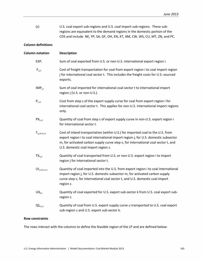
June 2013


(z) U.S. coal export sub-regions and U.S. coal import sub-regions. These sub- regions are equivalent to the demand regions in the domestic portion of the CDS and include NE, YP, SA, GF, OH, EN, KT, AM, CW, WS, CU, MT, ZN, and PC.

Column definitions

Column notation Description

EXPi Sum of coal exported from U.S. or non-U.S. international export region i.

Fi,j,t Cost of freight transportation for coal from export region i to coal import region j for international coal sector t. This includes the freight costs for U.S.-sourced exports.

IMPj,t Sum of coal imported for international coal sector t to international import region j (U.S. or non-U.S.).

Pi,s,t Cost from step s of the export supply curve for coal from export region i for international coal sector t. This applies for non-U.S. international import regions only.

PXi,s,t Quantity of coal from step s of export supply curve in non-U.S. export region i for international sector t.

Ti,j,m,t,v,z Cost of inland transportation (within U.S.) for imported coal to the U.S. from export region i to coal international import region j, for U.S. domestic subsector m, for activated carbon supply curve step v, for international coal sector t, and U.S. domestic coal import region z.

TXi,j,t Quantity of coal transported from U.S. or non-U.S. export region i to import region j for international sector t.

UIi,j.m,t,v,z Quantity of coal imported into the U.S. from export region i to coal international import region j, for U.S. domestic subsector m, for activated carbon supply curve step v, for international coal sector t, and U.S. domestic coal import region z.

UXk,z Quantity of coal exported for U.S. export sub-sector k from U.S. coal export sub- region z.

Qtk,u,z Quantity of coal from U.S. export supply curve u transported to U.S. coal export sub-region z and U.S. export sub-sector k.

Row constraints

The rows interact with the columns to define the feasible region of the LP and are defined below:

June 2013


U.S. IMPORTS STRUCTURE ONLY U.S. IMPORT EQUATIONS: non-imported coal + Σi,v UIi,j.m,t,v,z = Dj,m,t,z (3.B-2)

where Dj,m,t,z represents the U.S. coal imports for coal import region j, U.S. subsector m, for international coal sector t, and for U.S. domestic coal demand region z. DEFINITION: Specifies the level of coal imports by import region j that must be satisfied for domestic coal subsector m. CORRESPONDING ROWS IN BLOCK DIAGRAM: D.(DR)(PT), D.(DR)I(SN) and D.(DR)M(SN)

BALANCE OF U.S. INLAND TRANSPORTATION AND INTERNATIONAL FREIGHT TO U.S. EQUATIONS: TXi,j,t - Σm,v,z UIi,j.m,t,v,z = 0 (3.B-3) DEFINITION: For j equal to U.S. importing regions, the row balances coal freighted to U.S. international import region j from international (non-U.S.) export region i for international sector t (thermal or coking).

CORRESPONDING ROWS IN BLOCK DIAGRAM: TTU(UP)(ISR)XX and TCU(UP)(ISR)XX SULFUR DIOXIDE EMISSION RESTRICTION CONSTRAINTS: SO2 emissions from non-imported coal + Σi,j,m,t,v,z [si,,t* UIi,j.m,t,v,z] ≤ S (3.B-4) DEFINITION: For t equal to thermal coal, and for the subscript m representing electricity subsectors only, this row restricts the sulfur dioxide levels of coal in the U.S. electricity sector such that the sulfur dioxide emissions limit, “S,” is met and “si,t” equals the sulfur dioxide content of the coal from international supply region i in sector t. For more detail on sulfur dioxide emissions from non-imported coal, see “2. Coal Distribution Submodule – Domestic Component.”

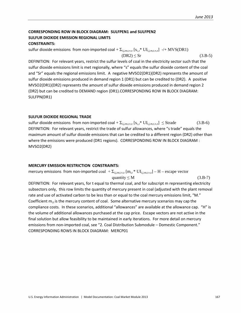
June 2013


CORRESPONDING ROW IN BLOCK DIAGRAM: SULFPEN1 and SULFPEN2 SULFUR DIOXIDE EMISSION REGIONAL LIMITS CONSTRAINTS: sulfur dioxide emissions from non-imported coal + Σi,j,m,t,v,z [si,,t* UIi,j.m,t,v,z] -/+ MVS(DR1) (DR2) ≤ Sr (3.B-5) DEFINITION: For relevant years, restrict the sulfur levels of coal in the electricity sector such that the sulfur dioxide emissions limit is met regionally, where “s” equals the sulfur dioxide content of the coal and “Sr” equals the regional emissions limit. A negative MVSO2(DR1)(DR2) represents the amount of sulfur dioxide emissions produced in demand region 1 (DR1) but can be credited to (DR2). A positive MVSO2(DR1)(DR2) represents the amount of sulfur dioxide emissions produced in demand region 2 (DR2) but can be credited to DEMAND region (DR1).CORRESPONDING ROW IN BLOCK DIAGRAM: SULFPN(DR1)

SULFUR DIOXIDE REGIONAL TRADE sulfur dioxide emissions from non-imported coal + Σi,j,m,t,v,z [si,,t* UIi,j.m,t,v,z] ≤ Strade (3.B-6) DEFINITION: For relevant years, restrict the trade of sulfur allowances, where “s trade” equals the maximum amount of sulfur dioxide emissions that can be credited to a different region (DR2) other than where the emissions were produced (DR1 regions). CORRESPONDING ROW IN BLOCK DIAGRAM : MVSO2(DR2)

MERCURY EMISSION RESTRICTION CONSTRAINTS: mercury emissions from non-imported coal + Σi,j,m,t,v,z [mi,t * UIi,j.m,t,v,z] – H – escape vector quantity ≤ M (3.B-7) DEFINITION: For relevant years, for t equal to thermal coal, and for subscript m representing electricity subsectors only, this row limits the quantity of mercury present in coal (adjusted with the plant removal rate and use of activated carbon to be less than or equal to the coal mercury emissions limit, “M.” Coefficient mi,t is the mercury content of coal. Some alternative mercury scenarios may cap the compliance costs. In these scenarios, additional “allowances” are available at the allowance cap. “H” is the volume of additional allowances purchased at the cap price. Escape vectors are not active in the final solution but allow feasibility to be maintained in early iterations. For more detail on mercury emissions from non-imported coal, see “2. Coal Distribution Submodule – Domestic Component.” CORRESPONDING ROWS IN BLOCK DIAGRAM: MERCP01

June 2013


ACTIVATED CARBON SUPPLY CURVE CONSTRAINTS: activated carbon used with non-imported coal + Σi,j,m,t,v,z [ap,v* UIi,j.m,t,v,z] – 10 * Σv Av ≤ 0 (3.B-8) DEFINITION: Balances the activated carbon used in association with the electricity sector transportation vectors with the activated carbon supply curves. Coefficient ap,v represents tons of activated carbon per trillion Btu for plant configuration p and activated supply curve step v. “Av” represents the total quantity of activated carbon from activated carbon supply curve step v. For more detail on activated carbon use from non-imported coal, see “2. Coal Distribution Submodule – Domestic Component.” CORRESPONDING ROWS IN BLOCK DIAGRAM: ACIXXXXY

CARBON TAX CONSTRAINTS: carbon emissions from non-imported coal + Σi,j,m,t,v,z [ci,m* UIi,j.m,t,v,z] – C ≤ 0 (3.B-9) DEFINITION: Balances the carbon emissions, “C,” associated with the electricity sector transportation vectors with the carbon emissions being “paid for” with the carbon penalty price. Coefficient ci,m is the carbon content of coal from non-U.S. export region i and U.S. domestic subsector m. For more detail on carbon emissions from non-imported coal, see “2. Coal Distribution Submodule – Domestic Component.” CORRESPONDING ROWS IN BLOCK DIAGRAM: CARBONXX

HISTORICAL FLOW CONSTRAINTS: MINIMUM IMPORT EQUATION: Σi,j,m,t,v,z UIi,j.m,t,v,z ≥ T1 (3.B-10) DEFINITION: Sets minimum value (T1) for all U.S. imports. CORRESPONDING ROWS IN BLOCK DIAGRAM: IMPSTMIN

MAXIMUM IMPORT EQUATION: Σi,j,m,t,v,z UIi,j.m,t,v,z ≤ T2 (3.B-11) DEFINITION: Sets maximum value (T2) for all U.S. imports. CORRESPONDING ROWS IN BLOCK DIAGRAM: IMPSTMAX

MINIMUM METALLURGICAL IMPORT EQUATION: Σi,j,m,t,v,z UIi,j.m,t,v,z ≥ T3 (3.B-12) DEFINITION: For subscript t set equal to coking coal and m representing metallurgical subsectors only, sets minimum value (T3) for metallurgical imports. CORRESPONDING ROWS IN BLOCK DIAGRAM: IMPMETSW

June 2013


MINIMUM INDUSTRIAL IMPORT EQUATION: Σi,j,m,t,v,z UIi,j.m,t,v,z ≥ T4 (3.B-13) DEFINITION: For subscript t set equal to thermal coal and m representing industrial subsectors only, sets minimum value (T4) for industrial imports. CORRESPONDING ROWS IN BLOCK DIAGRAM: IMPINDSW

MINIMUM ELECTRICITY IMPORT EQUATION: Σi,j,m,t,v,z UIi,j.m,t,v,z ≥ T5 or T6 (3.B-14) DEFINITION: For subscript t set equal to thermal coal, m representing electricity subsectors only, sets minimum value (T5 for scrubbed or T6 for unscrubbed plants) for electricity imports. CORRESPONDING ROWS IN BLOCK DIAGRAM: F(ISR)(DR)I1 AND C(ISR)(DR)I1

WORLD COAL TRADE ROWS NON-U.S. PRODUCTION/SHIPPING BALANCE EQUATIONS: Σs PXi,s,t - Σj TXi,j,t = 0 (3.B-15) DEFINITION: Balance of coal produced in international (non-U.S.) export region i with the coal shipped from export region i for international sector t (thermal or coking). CORRESPONDING ROWS IN BLOCK DIAGRAM: SXX(ISR)(IDR)T and SXX(ISR)(IDR)C

NON-U.S. IMPORT EQUATIONS: Σi TXi,j,t = Dj,t (3.B-16)

where,

Dj,t represents the coal imports for import region j for international coal sector t. DEFINITION: Specifies the level of coal import requirement by import region j that must be satisfied for international coal sector t (thermal or coking). CORRESPONDING ROWS IN BLOCK DIAGRAM: DX(IDR)T and DX(IDR)C

U.S. AND NON-U.S. FREIGHT/IMPORT BALANCE EQUATIONS: Σi TXi,j,t - IMPj,t = 0 (3.B-17) DEFINITION: Balance of total coal imported to international import regions j with quantity freighted to import region j for international sector t. CORRESPONDING ROWS IN BLOCK DIAGRAM: BDX.(IDR)(IS)

June 2013


U.S. AND NON-U.S. IMPORT CONSTRAINTS: TXi,j,t - ICi,j,t*IMPj,t < 0 (3.B-18) DEFINITION: Import constraint specifying that only a certain share of imports for an import region j can come from export region i. ICi,j,t is the proportion of coal imports flowing to internatonal import region j that can come from export region i for international coal sector t.

CORRESPONDING ROWS IN BLOCK DIAGRAM: VI(IDR)(IS)(ISR)

U.S. AND NON-U.S. PRODUCTION/EXPORT BALANCE EQUATIONS: aΣs PXi,s,t + bΣk,z UXk,z - EXPi,t = 0, (3.B-19) where a = 0 and b = 1, for U.S.; a = 1 and b = 0 for non-U.S.; and where k is a subset of t. DEFINITION: Balance of coal produced for export from international export region i with total exported from i for international sector t. CORRESPONDING ROWS IN BLOCK DIAGRAM: BSXUS and BSX(ISR)

U.S. EXPORT BALANCE EQUATIONS: Σk,z UXk,z - Σj TXi,j,t = 0, (3.B-20)

where z is a subset of i and k is a subset of t. DEFINITION: Balance of total U.S. coal transported overseas with U.S. coal exported. The U.S. export requirement is bounded. The bounds assumed are based on historical levels of exports. CORRESPONDING ROWS IN BLOCK DIAGRAM: SDX(UXSR)(UXS)

U.S. EXPORT BALANCE EQUATIONS: Σu Qtk,u,z - UXk,z = 0 (3.B-21) Definition: Balance of coal transported within U.S. from U.S. coal supply curves to meet export requirements from U.S. export sub-regions z and U.S. export sub-sectors k. The U.S. export requirements are bounded. The bounds are based on historical levels of exports. CORRESPONDING ROWS IN BLOCK DIAGRAM: D.(UXSR)X(UXS)

U.S. AND NON-U.S. EXPORT CONSTRAINT CONSTRAINTS: TXi,j,t - ECi,j,t*EXPi < 0 (3.B-22)

Definition: Export constraint limiting the amount of export coal from an international export region i that can be shipped to a particular import region j. ECi,j,t is the proportion of coal exports flowing from internatonal export region i that can be shipped to import region j for international coal sector t.

CORRESPONDING ROWS IN BLOCK DIAGRAM: VE(ISR)(IDR)(IS)

June 2013


Table 3.B-2. Row and Column Structure of the International Component of the Coal Market Module

Each column and row of the linear programming matrix is assigned a name identifying the activity or constraint that it represents. A mask defines the general or generic name of a set of related activities or constraints. For example, the mask ‘PX(ISR)(IS)’ defines the general name of all activities representing the production of coal from international export regions. The names of specific activities or constraints are formed by inserting into the mask appropriate members of notational sets identified by the mask. For instance, the production of coal in Australia is defined as PX(AS)(T).

Table 3.B.2. Row and column structure of the international component of the coal market module


ACIXSS(STEPS)Y Column Volume of activated carbon (in pounds) injected to reduce mercury

emissions; column bounds on this vector are present specifying how much

activated carbon is available at each step

ACIXXXXY Column Assigns activated carbon requirement (pounds of activated carbon per

trillion Btu) for each activated carbon step in transportation column

BDX(IDR)(IS) Row Imports balance row for international import region (IDR) for international

coal sector (IS)

BSX(ISR) Row Export balance row for export region (ISR)

BSXUS Row Balance row for U.S. exports

CARBONXX Column Assigns carbon tax to coal in carbon scenario and influences patterns of coal

use in electricity sector

CARBONXX Row Assigns carbon content to electricity sector transportation columns

C(ISR)(DR)I1 Row Sets minimum level for U.S. electricity imports for unscrubbed plants by

export region (ISR) to U.S. demand region (DR)

D.(DR)I(SN) Row Coal demand from demand region (DR) for industrial sector, I, and sector

number (SN)

D.(DR)M(SN) Row Coal demand from demand region (DR) for metallurgical sector, M, and

sector number (SN)

D.(DR)(PT) Row Coal demand from demand region (DR) for electricity plant types (PT)

D.(UXSR)X(UXS) Row Export balance row for U.S. export sub-region (UXSR) of U.S. export sub-

sector (UXS)

DX.(IDR)C Row Import row for import region (IDR) and international coking coal sector

DX.(IDR)T Row Import row for import region (IDR) and international thermal coal sector

EXP(ISR) Column Sum of exports from export region (ISR)

F(ISR)(DR)I1 Row Sets minimum level for U.S. electricity imports for scrubbed plants by export

region (ISR) to U.S. demand region (DR)

IMP(IDR)(IS) Column Sum of imports from import region (IDR) for international coal sector (IS)

June 2013


Table 3.B-2. Row and column structure of the international component of the coal market module (cont.)


IMPINDSW Row Sets minimum level for industrial imports for a given year

IMPMETSW Row Sets minimum level for metallurgical imports for a given year

IMPSTMAX Row Sets maximum level for total imports for a given year

IMPSTMIN Row Sets minimum level for total imports for a given year

MERCEV Column Provides upper bound for mercury allowance price

MERCP01 Row Mercury penalty constraint for electricity sector

MOREHGXX Column Escape vector allowing more mercury to be emitted if tight mercury

constraint causes infeasibility. Not active in final solution.

MVS(DR1)(DR2) Column Specifies sulfur dioxide emissions trade from demand region 1 to

demand region 2

MVSO2(DR2) Row Specifies the overall limits to trade in sulfur dioxide emissions by the

destination region (where the emissions are transferred to)

OII(SN)(ISR)T(DR) Column U.S. import volume transported within the U.S. for use in the

industrial steam sector

OIM(SN)(ISR)C(DR) Column U.S. import volume transported within the U.S. for in the

metallurgical sector

PX.(ISR)(IS)(STEPS) Column Supply of exports for non-U.S. international export region (ISR) for

international coal sector (IS) and supply curve step (STEPS)

SDX(UXSR)(UXS) Row Row balancing the sum of coal transported from the export

subsectors (UXS) from the international U.S. export region (UXSR)

with the total exported from the U.S. export region (UXSR)

SULFPEN1 Row Sulfur penalty constraint for the East for electricity sector

SULFPEN2 Row Sulfur penalty constraint for the West for electricity sector

SULFPN(DR1) Row Specifies regional sulfur dioxide limit by demand region

SXX(ISR)(IDR)C Row Row balancing the supply of coal exports from international export

region (ISR) to international import region (IDR) for coking coal

SXX(ISR)(IDR)T Row Row balancing the supply of coal exports from international export

region (ISR) to international import region (IDR) for thermal coal

TCU(UP)(ISR)XX Row Row balancing the quantity of imported coking coal transported

inland from U.S. port (UP) from international export region (ISR) to

that freighted to the port from international export region (ISR)

TTU(UP)(ISR)XX Row Row balancing the quantity of imported thermal coal transported

inland from U.S. port (UP) from international export region (ISR) to

that freighted to the port from international export region (ISR)

T(USR)(UXSR)X(UXS)(CT) Column U.S. export volume transported internally from U.S. export regions

where coal is produced (USR) to U.S. export sub-regions (UXSR) for

U.S. export sub-sectors for coal type (CT)

June 2013


Table 3.B-2. Row and column structure of the international component of the coal market module (cont.)


TX(DR)X(UXS)(IDR)(IS) Column U.S. export transportation volume from U.S. export sub-region

(DR), to international import region (IDR), for U.S. export sub-

sector (UXS), for international export sector (IS)

TX(ISR)-(IDR)(IS) Column Export volume transported from non-U.S. export region (ISR) to

international import region (IDR) for international export sector

(IS)

UX(UXSR)-X(UXS) Column Export volume for U.S. export sub-region (UXSR) and U.S. export

sub-sector (UXS). Export volume must lie between an upper and

lower bound derived from historical volumes.

VE(ISR)(IDR)(IS) Row Diversity export constraint on international export region (ISR) to

import region (IDR) for international export sector (IS)

VI(IDR)(IS)(ISR) Row Diversity import constraint on import region (IDR) for international

export sector (IS) from export region (ISR)

where,

CT U.S. DOMESTIC COAL TYPE (CT’s pairing with a U.S. supply region designates the supply curve and rank.)

1 LOW SULFUR AND UNDERGROUND MINING METHOD 2 MEDIUM SULFUR AND UNDERGROUND MINING METHOD 3 HIGH SULFUR AND UNDERGROUND MINING METHOD 4 LOW SULFUR AND SURFACE MINING METHOD 5 MEDIUM SULFUR AND SURFACE MINING METHOD 6 HIGH SULFUR AND SURFACE MINING METHOD 7 METALLURGICAL COAL 8 WASTE COAL OR MISSISSIPPI LIGNITE

DR or UXSR U.S. EXPORT SUB-REGIONS AND/OR U.S. IMPORT REGIONS NE CONNECTICUT, MASSACHUSETTS, MAINE, NEW HAMPSHIRE, RHODE ISLAND, VERMONT YP NEW YORK, PENNSYLVANIA, NEW JERSEY SA WEST VIRGINIA, DELAWARE, DISTRICT OF COLUMBIA, MARYLAND, VIRGINIA, NORTH CAROLINA, SOUTH CAROLINA GF GEORGIA, FLORIDA OH OHIO EN ILLINOIS, INDIANA, MICHIGAN, WISCONSIN KT KENTUCKY, TENNESSEE AM ALABAMA, MISSISSIPPI CW MINNESOTA, IOWA, NORTH DAKOTA, SOUTH DAKOTA, NEBRASKA, KANSAS, MISSOURI WS TEXAS, OKLAHOMA, ARKANSAS, LOUISIANA MT MONTANA, WYOMING, IDAHO

June 2013


CU COLORADO, UTAH, NEVADA ZN ARIZONA, NEW MEXICO PC ALASKA, HAWAII, WASHINGTON, OREGON, CALIFORNIA

IDR INTERNATIONAL IMPORT REGIONS NE East Coast Canada NI Interior Canada SC Scandinavia BT United Kingdom, Ireland GY Germany, Austria OW Other Northern Europe PS Iberian Peninsula IT Italy (thermal and coking) RM E. Europe and Mediterranean MX Mexico LA South America JA Japan EA East Asia CH China, Hong Kong AS ASEAN IN Indian Subcontinent, S. Asia UE U.S. Eastern UG U.S. Gulf UI U.S. Interior UN U.S. Noncontiguous

IS INTERNATIONAL COAL SECTORS C Coking T Thermal

ISR INTERNATIONAL EXPORT REGIONS NA Canada (alternate for Canada) NW or W West Coast Canada NI or N Interior Canada (thermal only) CL or C Colombia (thermal only) VZ or Z Venezuela (thermal only) PO or P Poland RE or E Former Soviet Union (exports to Europe) RA or R Former Soviet Union (exports to Asia) SF or S Southern Africa IN or I Indonesia HI or H China AU or A Australia VT or T Vietnam

June 2013


US U.S. UA U.S. All UG U.S. Gulf UI U.S. Interior UN U.S. Noncontiguous UW U.S. West coast UE U.S. East coast

PT PLANT TYPE (see CDS – Domestic Component, page 68)

SN U.S. IMPORT SUB-SECTOR NUMBERS

1 – 3 FOR INDUSTRIAL IMPORTS 1 – 2 FOR METALLURGICAL IMPORTS

STEPS INTERNATIONAL EXPORT SUPPLY CURVE STEPS or ACTIVATED CARBON STEP

1 Step 1 2 Step 1 3 Step 3 4 Step 4 5 Step 5 6 Step 6 7 Step 7 8 Step 8 9 Step 9 0 Step 10

UP U.S. PORT REGION G U.S. Gulf I U.S. Interior N U.S. Noncontiguous E U.S. East coast

USR U.S. COAL SUPPLY REGIONS NA PENNSYLVANIA, OHIO, MARYLAND, WEST VIRGINIA (NORTH) CA WEST VIRGINIA (SOUTH), KENTUCKY (EAST), VIRGINIA, TENNESSEE (NORTH) SA ALABAMA, TENNESSEE (SOUTH) EI ILLINOIS, INDIANA, KENTUCKY (WEST), MISSISSIPPI WI IOWA, MISSOURI, KANSAS, OKLAHOMA, ARKANSAS, TEXAS (BITUMINOUS) GL TEXAS (LIGNITE), LOUISIANA DL NORTH DAKOTA, MONTANA (LIGNITE) WM WESTERN MONTANA (SUBBITUMINOUS) NW WYOMING, NORTHERN POWDER RIVER BASIN (SUBBITUMINOUS) SW WYOMING, SOUTHERN POWDER RIVER BASIN (SUBBITUMINOUS)

June 2013


WW WESTERN WYOMING (SUBBITUMINOUS) RM COLORADO, UTAH ZN ARIZONA, NEW MEXICO AW WASHINGTON, ALASKA

UXS U.S. EXPORT SECTORS 1 Metallurgical Export 1 2 Metallurgical Export 2 3 Metallurgical Export 3 4 Steam 1 Export 5 Steam 2 Export 6 Steam 3 Export

USXR U.S. EXPORT SUB-REGIONS AND/OR U.S. IMPORT REGIONS See DR.

June 2013


Appendix 3.C. Inventory of Input Data, Parameter Estimates, and Model Outputs Model inputs

The inputs required by the international component of the CDS are divided into two main groups: user-specified inputs and inputs provided by other NEMS components. The required user-specified inputs are listed in Table 3.C-1. In addition to identifying each input, this table indicates the variable name used to refer to the input in this report, the units for the input, and the level of detail at which the input needs to be specified.

The user-specified inputs to the international component of the CDS are contained in six different input files. These files and their contents are listed below.

CLEXSUP. This file contains the step-function coal export supply curves for all non-U.S. export regions. The first column contains the international export region and step identifier. The next seven columns contain the variables:

1) FOBYR, the export FOB price of coal (minemouth price plus inland transportation cost) in 1992 dollars per metric ton for 1992; 2) CAPYR, the estimated coal export capacity in million metric tons for 1992; 3) CV, the heat content in thousand Btu per pound for all forecast years; 4) SULCON, the sulfur content in percent sulfur by weight for all forecast years; 5) IMPMERC, the mercury content in pounds per trillion Btu; 6) IMPCO2, the carbon dioxide content in pounds of carbon dioxide per million Btu; and 7) SCALAR, a scalar that permits the user to adjust the international coal export supply curves over time at rates that vary from the price path for U.S. export coal.

The remaining columns contain estimates of export prices (FOBYR) and capacities (CAPYR) for each of the coal export supply steps represented in the CDS for the remaining forecast years (typically specified at 5-year intervals).

Some additional calculations are required to convert input data from the file to units consistent with the linear program. They include:

• Conversion of FOBYR to 1987 dollars per trillion Btu using the following calculation: FOBYR * 12.6 thousand Btu per pound of coal equivalent / CV * 1987 GDP deflator/1992 GDP deflator / 27.78 mmBtu per metric ton of coal equivalent

or equivalently, FOBYR * 1987 GDP deflator/ 1992 GDP deflator/ 2204.623 pounds per metric ton/ CV * 103

June 2013


• Conversion of CAPYR, coal export capacity, to trillion Btu using the following calculation: CAPYR * CV /12.6 thousand Btu per pound of coal equivalent * 27.78 mmBtu per metric ton of coal equivalent or equivalently, CAPYR * 2204.623 pounds per metric ton * CV / 103.

• Conversion of SULCON to thousand tons of SO2 per trillion Btu by the following calculation: SULCON * 10.0 / CV.

• Conversion of IMPCO2 to million metric tons of carbon per quadrillion Btu by the following calculation: IMPCO2 * 12.0/ 44.0 /2.204623 or equivalently, IMPCO2 * 12.0/ 44.0/ 2204.623 pounds per metric ton * 103.

CLEXDEM. This file contains the non-U.S. coal import requirements (variable: DEMAND) by international CDS import region and sector for the years 1990 through 2050 (typically specified at five-year intervals). The first column in the file indicates the year for the import requirements contained in each row of the file. The remaining columns contain the coal import requirements in million metric tons of coal equivalent for each specific combination of international CDS import region (including the United States) and demand sector (e.g., JAC represents coking coal imports to Japan, and JAT represents thermal coal imports to Japan). Prior to use in the LP, the import requirements are converted to trillion Btu by the following calculation: DEMAND * 27.78 million Btu per metric ton of coal equivalent.

CLEXFRT. This file contains a matrix of ocean transportation rates (variable: FREIGHT) for coal shipments. The transportation rates are specified by international CDS import region, export region, and demand sector (coking and thermal). Each column heading represents a specific international CDS import region, and each row represents a specific combination of international CDS export region and demand sector. The rates are specified in 1992 dollars per metric ton. Prior to use in the LP, the ocean transportation rates are converted to 1987 dollars per million Btu.

This file also contains inland transportation rates (variable: INLANDTR), in 1987 dollars per short ton, for U.S. imports. These rates represent the transportation cost from the initial import entry to the U.S. coal import region and are specified by the electricity, industrial, and metallurgical sectors. This file also includes optional switches to set minimum and/or maximum import levels. If a switch is equal to “1,” the minimum/maximum constraint is in use.

CLEXEXS. This file contains international requirements for U.S. coal export levels for the historical and Short-Term Energy Outlook years of the forecast.26 Each row includes five indices at the left followed by a set of numbers representing annual U.S. coal exports in trillion Btu for the years 1990 through 2013. From left to right these indices are (1) the domestic CDS demand region, (2) the international CDS demand sector, (3) the domestic CDS economic subsector, (4) the CDS coal group from which supplies 26 In general, the U.S. Energy Information Administration’s Short-Term Energy Outlook provides forecasts of U.S. coal exports for the period extending two years beyond the most recently published set of annual historical data.

June 2013


may be drawn (the organization of "coal groups" is explained in the discussion of the "CLPARAMS" input file in Appendix 2.C of Section 2 of the CMM Model Documentation), and (5) the international coal export region to which they pertain.

CLEXIMS. This file contains the coal import diversity constraints specified as a percent of the total coal imports. Each column heading represents a specific combination of international CDS import region and demand sector (coking and thermal), and each row represents a specific international CDS export region. The constraints limit the portion of an import region’s import requirement by sector that can be met by each of the individual export regions. For example, an input of 40 for the JAT import region/sector and U.S. export region combination indicates that only 40 percent of Japan’s annual imports of thermal coal can be met by U.S. coal suppliers.

CLEXSO2. This file contains the constraints for high-sulfur coal, subbituminous coal, and sulfur dioxide emissions. The first column of the file identifies the specific constraints as follows: High-Sulfur Percent (variable: HSPCT): portion of an international CDS import region’s thermal coal import requirement that can be met by high-sulfur coal; Subbituminous Percent: portion of an international CDS import region’s thermal coal import requirement that can be met by subbituminous coal; Percent Low-Sulfur Coal Scrubbed: portion of an international CDS import region’s low-sulfur coal import requirement that is scrubbed; Percent High-Sulfur Coal Scrubbed: portion of an international CDS import region’s high-sulfur coal import requirement that is scrubbed; Sulfur Cap: cap on sulfur dioxide emissions specified in thousand metric tons. The remaining columns contain the corresponding data for each of the constraints for each international CDS import region. These constraints were not used for AEO2013.

CLCONT. See Section 2’s Appendix 2.C.

Model outputs

The international component of the CDS provides annual forecasts of U.S. coal exports and imports to the domestic distribution area of the NEMS Coal Market Module. The key output from international area of the CDS, listed in Table 3.C-2, is world coal trade flows by coal export region/coal import region/coal type/coal demand sector (in trillion Btu). Conversion factors convert output from trillion Btu to short tons for report-writing purposes.

June 2013


Table 3.C-1. User-specified inputs

CDS

Variable Input Specification Levela Input Units

CAPYR Coal export capacity Coal export region/coal sector/export supply curve

step/forecast year

Million metric tons

CV Btu conversion assignment

for coal export supply curve

Coal export region/coal sector/export supply curve step Thousand Btu per pound

of coal

DEMAND Coal import requirement

(Non-U.S.)

Coal import region/coal demand sector/forecast year Million metric tons of

coal equivalent

EXPSHARE Exporter diversity constraints Coal export region/coal import region Percentage

FOBYR Coal export prices (FOB port

of exit)

Coal export region/coal sector/export supply curve

step/forecast year

1992 dollars per metric

ton

FREIGHT Ocean freight rates Coal export region/coal import region/coal sector/coal

demand sector

1992 dollars per metric

ton

HSMAXb Maximum share of high-sulfur

coal imports

Coal import region/forecast year Fraction

HSPCTb SO2 emissions "pass-through"

rate

Coal import region/coal demand sector/forecast year Fraction

INLANDTR Inland coal transportation

rates for U.S. coal imports

U.S. sector/U.S. domestic demand region/international

export region/U.S. port of entry

1987 dollars per short

ton

IMPMERCc Mercury content assignment

for coal export supply curve

Coal export region/coal type Pounds of mercury per

trillion Btu

IMPSHARE Importer diversity constraints Coal export region/coal import region Percentage

IMPCO2c Carbon dioxide content

assignment for coal export

supply curve

Coal export region/coal type Pounds of CO2 per

million Btu

LSPCTb SO2 emissions "pass-through"

rate

Coal import region/coal demand sector/forecast year Fraction

MAXSULb Limit on total SO2 emissions

for international trade

Coal import region/forecast region Thousand metric tons

SCALINT Price adjustment factor for

non-U.S. export supply curves

Coal export region/coal type/export supply curve

step/forecast year

Scalar

SUBMAXb Maximum share of

subbituminous coal imports

Coal import region/forecast year Fraction

SULCONc Sulfur content assignment for

coal export supply curve

Coal export region/coal type Thousand metric tons of

SO2 emissions per metric

ton of coal equivalent aFor example, inputs specified at the coal export region/coal sector/forecast year level require separate values for each export region, coal type, and forecast. bThese variables are not currently used. cUsed for U.S. imports.

June 2013


Table 3.C-2. Outputs

Input CDS Variable Specification Levela Units

World coal trade flows SOLVAL Coal export region/coal import

region/coal sector/coal demand

sector/forecast year

Trillion Btu

June 2013


Appendix 3.D. Data Quality and Estimation Non-U.S. coal import requirements are import volumes specified by CDS international coal import region and demand sector (coking and thermal). Annual import requirements are assumed to be equal to domestic coal demand less domestic supply (domestic production minus exports). In the CDS, non-U.S. coal import requirements by region and international import sector are an exogenous input, and are typically specified at five-year intervals. Published information such as announced and planned additions/retirements of coal-fired generating plants, coke plants, and coal mining capacity are used to adjust the annual input data for coal import requirements. Annual coal import requirements for the years not specified in the CLEXDEM input file are determined by linear interpolation.

Coking coal requirements represent the consumption of coal at coke plants to produce coal coke. Coal coke is used primarily as a fuel and as a reducing agent in smelting iron ore in a blast furnace. Coal coke is also consumed at foundries and in the production of sinter. Thermal coal demands correspond to coal consumed for electricity generation, industrial applications (excluding the use of coking coal at coke plants), space heating in the commercial and residential sectors, and for the production of coal-based synthetic gas and liquids. The direct use of coal at blast furnaces for the manufacture of pig iron is also categorized as thermal coal demand.

Coal export supply inputs are potential export supplies specified on a tranche-by-tranche (steps on supply curve) basis in the clexsup.txt input file to enable users to build up a stepped supply curve. Up to ten tranches are allowed for the major price-sensitive suppliers. Coal qualities (sulfur, mercury, carbon dioxide and Btu content) cannot vary between tranches.

With each update of the AEO, the export FOB price of coal (FOBYR) for the international base year (2011) is updated on the basis of available data on average annual prices for coal exports and imports as reported by EIA, the International Energy Agency, South Africa’s Department of Minerals and Energy, and other statistical agencies and organizations. For international export supply regions and coal types where data for average annual coal export prices are either limited or unavailable, prices are updated on the basis of changes in reported prices for other coal export regions. Further adjustments are made to calibrate the model to base-year trade flows.

The FOBYR and CAPYR variables together represent the supply curves for each of the modeled supply regions. For the base year, the paired variables represent estimates of current coal supply potential while projection years consider known capacity plans and capacity potential both in regards to mine capacity expansions (for exported coal), reserves, inland transportation upgrades, and port capacity upgrades or limitations. Limited availability and consistent sources of reliable international data present a difficulty in updating these assumptions. The update of these curves ultimately requires some judgment on the part of the modeler. In general, the slope of these supply curves is assumed to be similar to those of the United States. The SCALINT variable allows productivity assumptions to differ from those of the United States for the various supply curves. Assumptions about the elasticity of coal export supply for each exporting country determine the prices associated with steps on the supply curves representing new mine capacity.

June 2013


International freight shipping costs start from a matrix of feasible export routes, and taking into account the maximum vessel sizes that can be handled at export and import piers and through canals, a matrix of maximum vessel sizes allowable on each route is generated. Freight rates are then calculated on the basis of route distance and vessel size, using the following set of formulas:

Handysize (vessel size < 55,000 dwt)

Rate (1992 dollars/tonne) = (2.5 + 1.5*D) * (1992 GDP deflator/1997 GDP deflator)

Panamax (vessel size ≥ 55,000 but < 80,000 dwt)


Capesize (vessel size ≥ 80,000 dwt)


where

D = distance in thousand nautical miles (1 nautical mile = 6076.115 feet) Tonne = metric ton (2204.623 pounds) dwt = deadweight ton (2240 pounds)

Users can adjust freight rates using an add-factor matrix to take account of backhaul savings, canal tolls, slow unloading terms, etc. This add-factor matrix incorporates a $2.00/t "washery credit" which is subtracted from every freight rate between a coking coal supplier and a thermal coal buyer.

U.S. import inland transportation rates for origin (port of entry) and destination (domestic coal demand regions) pairs are estimated using information about domestic shipping rates for comparable distances. Transportation rates were also adjusted in order to improve estimates of historical import volumes.

June 2013


Appendix 3.E. Optimization and Modeling Library (OML) Subroutines and Functions This appendix provides a summary of the OML routines that are called by the CDS to set up the database, revise coefficients, solve the LP model, and retrieve the solution. OML is a proprietary software package developed by KETRON Management Science.

DFOPEN: Opens the data file for the LP problem

DFPINIT: Initializes processing of the LP problem in the current database

DFMINIT: Initializes a database for matrix processing

DFMEND: Terminates matrix processing

DFCLOSE: Terminates processing of a database file

WFDEF: Defines the model space for the LP problem

WFLOAD: Loads the matrix for the LP problem into memory

WFINSRT: Loads the starting basis for the LP problem

WFOPT: Optimizes the model

WFPUNCH: Saves the current basis into a standard format file

DFMRRHS: Retrieves a right-hand side value

DFMCRHS: Creates or changes a right-hand side value

DFMRBND: Retrieves a bound value

DFMCBND: Creates or changes a bound value

DFMCVAL: Creates or changes a coefficient for a row/column intersection

DFMMVAL: Changes a coefficient for row/column intersection if it exists

DFMCRTP: Declares or changes the row type

WFSCOL: Retrieves solution values (e.g., activity, input cost, reduced cost) for a column vector

WFSROW: Retrieves solution values (e.g., activity, dual values) for a row

WFRNAME: Retrieves a row name

WFCNAME: Retrieves a column name

June 2013


Appendix 3.F. Bibliography Ellerman, Dr. A. Denny, Charles River Associates, Independent Expert Review of International Coal Trade Model Version 2 (ICTM-2) prepared for the U.S. Energy Information Administration (Washington, DC, June 1989).

U.S. Energy Information Administration, Annual Prospects for World Coal Trade 1991, DOE/EIA-0363(91) (Washington, DC, June 1991) and prior issues.

U.S. Energy Information Administration, Description of the International Coal Trade Model, DOE/EIA/11815-1 (Washington, DC, September 1982).

U.S. Energy Information Administration, Directory of Energy Information Administration Models 1992, DOE/EIA-0293(92) (Washington, DC, June 1992).

U.S. Energy Information Administration, International Coal Trade Model: Executive Summary, DOE/EIA-0444(EX) (Washington, DC, May 1984).

U.S. Energy Information Administration, International Coal Trade Model, Version 2, Preliminary Description, by William Orchard-Hayes, June 10, 1985.

U.S. Energy Information Administration, International Coal Trade Model—Version 2 (ICTM-2) User's Guide (Washington, DC, March 1987).

U.S. Energy Information Administration, Mathematical Structure of the International Coal Trade Model, DOE/NBB-0025 (Washington, DC, September 1982).

U.S. Energy Information Administration, Working Paper Requirements for a National Energy Modeling System (Washington, DC, May 18, 1992).

The George Washington University, Department of Operations Research, Oligopoly Theories and the International Coal Trade Model, GWU/IMSE/Serial T-494/84, by James E. Falk and Garth P. McCormick (Washington, DC, July 1984).

National Research Council, The National Energy Modeling System (Washington, DC, January 1992).

Resource Economics Corporation, WOCTES—World Coal Trade Expert System (Urbana, IL, 1992).

coal market module of the national energy modeling system model

Documents