1

Coal, Smoke, and Death:

Bituminous Coal and American Home Heating, 1920-1959

Alan Barreca, Tulane University

Karen Clay, Carnegie Mellon University and NBER

Joel Tarr, Carnegie Mellon University

December 2012

Preliminary and Incomplete, Please Do Not Quote Without Permission

Air pollution was severe in many parts of the United States in the first half of the twentieth century. Much of the air

pollution was attributable to bituminous coal. This paper uses newly digitized state-month mortality data to estimate

the effects of bituminous coal consumption for heating on mortality rates in the U.S. between 1920 and 1959. The

use of coal for heating was high until the mid-1940s, and then declined sharply. The switch to cleaner fuels was

driven by plausibly exogenous changes in the availability of natural gas, the end of war-related supply restrictions,

and a series of coal strikes from 1946-1950. The identification strategy leverages the fact that coal consumption for

heating increases during cold weather. Specifically, the mortality effects are identified from differences in the

temperature-mortality response functions in state-years with greater coal consumption. Cold weather spells in high

coal state-years saw greater increases in the mortality rates than cold weather spells in low coal state-years. Our

estimates suggest that reductions in the use of bituminous coal for heating between 1945 and 1959 decreased

average annual mortality by 2.2-3.5 percent, January mortality by 3.2-5.1 percent, average annual infant mortality by

1.6-2.8 percent, and January infant mortality by 3.1-4.6 percent. Our estimates are likely to be a lower-bound, since

they only capture short-run relationships between coal and mortality.

We thank Leila Abu-Orf, Paula Levin, and Katherine Rudolph for excellent research assistance. We are grateful to

Olivier Deschenes, Price Fishback, Gary Libecap, Paulina Oliva Paul Rhode, Mel Stephens, and seminar

participants at the Economic History Association 2011 Meetings, Stanford University, University of California,

Santa Barbara, and University of Michigan for helpful comments. The infant birth data was digitized with financial

support from NIA grant P30-AG012810 through the NBER.

2

1. Introduction

Humans have used fuels for heating for millennia. These fuels caused indoor and outdoor

air pollution. The outdoor component was particularly significant in cities, where widespread

burning of fuels led to large concentrations in particulates. As wood began scarce, many

societies began to burn coal. In developing countries today, the use of coal for heating is causing

severe air pollution in cities (Almond et al 2009, Cohen et al 2004). The United States

experienced similar issues in large cities in the 1930s and 1940s (Eisenbud 1978, Tarr 1996, Tarr

and Clay 2012). London experienced killing ‘fogs’ or smogs from the 1850s on, and its most

famous fog in 1952 (Clay and Troesken 2010).

This paper uses newly digitized mortality data from the United States at the state-month

level to quantify the effects of changing coal use on overall mortality and on infant mortality.

The use of bituminous coal for heating was high from 1920 through the mid-1940s and then

began to decline sharply for arguably exogenous reasons. At its peak, more than 50 percent of

United States households used coal for home heating, and the vast majority, 66-86 percent of

these households used bituminous coal. The decline in the use of coal, which began in the mid-

1940s, was driven by coal strikes of the second half of the 1940s, the end of war-related supply

restrictions on oil and natural gas, increased supply via new long-distance pipelines, and the

availability of low-cost conversion units for furnaces.

Coal use for heating is likely to have had two countervailing effects on mortality. Greater

consumption of coal for heat is likely to have some “protective effect”, since indoor heating

reducing the physiological stress associated with cold temperatures. At the same time, the use of

coal for heating has a significant “air pollution effect”, which is increasing in population density.

Many residential coal users were located in dense urban areas, burned the coal at relatively low

3

temperatures, and had low chimneys, all of which increased population exposure to pollution. In

contrast to residential users, companies involved in manufacturing and electricity generation

tended to be located away from the most densely populated areas, burned coal at high

temperatures, and had higher smokestacks that allowed for dispersion of smoke across a much

wider area. An increase in coal consumption has a theoretically ambiguous effect on mortality,

when the protective effects and polluting effects are both relevant. However, the rapid adoption

of cleaner fuels in the 1940s is hypothesized to yield improvements in air quality and health

without sacrificing indoor heat.

Our identification strategy leverages variation in the interaction between weather and

bituminous coal consumption within states over time. As we explain in the background section,

the variation in coal consumption across states is most likely due to proximity to deposits across

states, and the variation in coal consumption over time is related to a series of shocks that

occurred in the mid-1940s that lead to rapid declines in the use of coal for home heating. These

historical facts bolster the causal interpretation of our estimates. The key variable in our

regression model is the estimated consumption of bituminous coal per capita interacted with

heating degree-days with a base of 65. In simple terms, the identifying variation comes from the

differences in the mortality response from the unusually cold winters in high- versus low-coal-

consumption states (or state-years). The controls include main effects for the coal consumption

and heating degree days, as well as state by month fixed effects, (national) year by month fixed

effects, and state-specific time trends. The coal consumption measures were interpolated from 5-

year estimates from the Historic Emissions of Sulfur and Nitrogen Oxides in the United States

from 1900 to 1980. Heating degree-day variables were constructed from daily weather station-

day temperature readings from the United States Historical Climatology Network.

4

Reductions in the use of bituminous coal for heating between 1945 and 1959 decreased

annual average mortality 2.2-3.5 percent, January mortality by 3.2-5.1 percent, annual average

infant mortality by 1.6-2.8 percent, and January infant mortality by 3.2-4.6 percent. Our results

are robust to a variety of specification checks, including using a heating degree day base of 50F;

using a two month moving average of heating degree days; and controlling for income, other

uses of bituminous coal, and these variables interacted with heating degree days. Also, we find

that states with higher consumption in 1920 experienced greater declines in temperature-

mortality response function after 1945 than states with lower coal consumption, which is

consistent with our estimates being driven by arguably exogenous post-1945 decline in coal

consumption. Our estimates are likely to be a lower-bound, since they only capture short-run

relationships between coal and mortality.

Our paper complements pollution-mortality studies that rely on contemporary data. Chay

and Greenstone (2003a, 2003b), Currie and Neidell (2005), Currie, Neidell, and Schmieder

(2009), Currie and Walker (2011), Knittel, Miller, and Sanders (2012) have examined the effect

of pollution on infant mortality in the U.S. in the late 20th

century. Arceo-Gomez, Hanna, Oliva

(2012) present results from Mexico, where particulate levels are roughly twice the levels in the

U.S. There is also a closely related epidemiology literature (Pope et al 2002 and Laden 2006).

Our paper examines infant and overall mortality in a period where winter urban particulate levels

are roughly eight times the levels in the U.S. in the late 20th

century and four times the levels in

Mexico. The levels experienced in the historical U.S. were more comparable to those

experienced in developing countries today (Almond et al., 2009, Cohen et al 2004).1

1 This paper also contributes to the small but expanding historical literature on fuel use and fuel transitions (Wright

1964, Herbert 1992, Castaneda 1999).

5

2. Coal

Figure 1 shows energy consumption by source in the U.S. economy as a whole. Until the

1880s, the primary source of fuel in the economy was wood. Wood was surpassed by coal in the

1880s and coal remained the dominant fuel source through the 1940s, when it was surpassed by

petroleum. Initially, anthracite coal from eastern Pennsylvania was dominant. As deposits west

of the Alleghenies were developed and transportation facilities improved, bituminous coal

became dominant.

Over this period, bituminous coal was used for many purposes. Figure 2 illustrates the

trends in consumption for four primary uses– heating, industrial production, electricity

generation and rail transportation. Consumption differs over time across the four uses.

Bituminous coal consumption for electricity rises fairly steadily. Bituminous consumption for

heating rises fairly steadily and then falls after 1945. Bituminous consumption for industrial

purposes is fairly volatile, peaking in the 1920s and again in the 1940s. Consumption by

railroads peaks in 1920, falls to 1935, increases in 1940 and 1945 and the resumes its decline.

Our identification strategy leverages the variation in coal consumption over time within states.

Bituminous coal, particularly bituminous coal for heating, was also considered a major

contributor to winter particulate pollution. In 1930 the U.S. Public Health Service received an

appropriation of $25,000 to study air pollution. As the introduction to the study noted, “In recent

years the pollution of the atmosphere by smoke and other impurities, especially in the larger

cities, has been the subject of much discussion. … There has been much discussion as to the

injurious effects of smoke upon health.”2 Given their limited resources, the goal of the 1930

study was solely to collect data on air quality in large American cities. Owens automatic air

2 Ives et al (1936), p. 1.

6

filters were run continuously in fourteen large U. S. cities beginning in July 1931. Total

suspended particulates (TSP) were also sampled, although with lower frequency, because of the

higher cost of data analysis. Analysis showed that TSP levels were highly correlated with the

shade of the Owens automatic air filter. Figure 4 shows that winter air quality was nearly twice

as bad as summer air quality. Average TSP in the winter months in these cities was 510. The

study explored heating’s contribution to pollution by examining pollution by time of day and by

comparing Sundays, when most businesses were shut, to weekdays. Both analyses suggested

that heating with coal was a major cause of pollution. Based on this analysis, the study concluded

“the nonindustrial pollution in the winter, resulting from the heating of residences, apartment

houses, hotels, and other buildings, appears to be a greater factor than the year-round industrial

pollution.”3 We return to this issue in a later section.

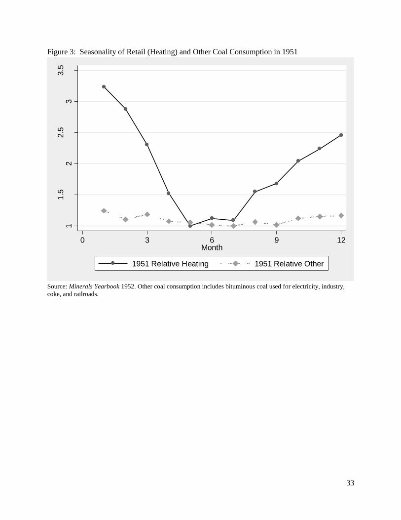
Figure 3 provides further evidence on the seasonality of consumption of retail coal, which

was used for heating and for hot water, and the seasonality of other coal uses, including

electricity generation, industrial production, and transportation. The Minerals Yearbook only

began reporting consumption by use by month in 1951.4 January consumption for retail coal was

more than three times the consumption in the lowest month, which typically falls in the May-July

window. In comparison, non-retail use was only slightly seasonal. Analysis of other years

indicates that the seasonality of coal consumption was fairly stable across the 1950s. This

suggests that consumption of retail coal followed similar patterns in the earlier period. Our

identification strategy also leverages the variation in coal consumption for heating across months

within states.

3 Ives et al (1936), p. 47.

4 Other years of data have similar seasonal relationships.

7

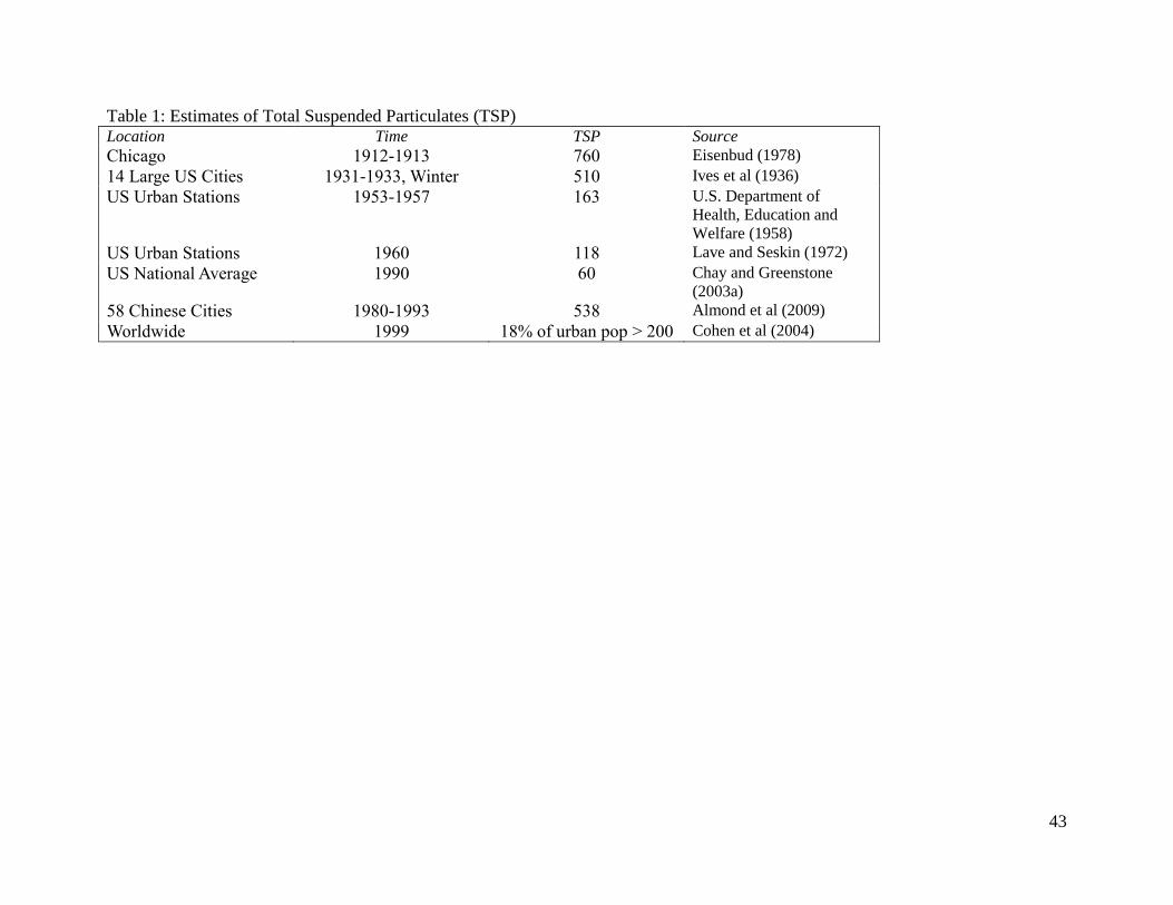
Table 1 presents selected estimates of particulate pollution in the United States and

developing countries. Particulates were not routinely measured in the United States until the late

1960s. While particulate pollution in the United States is currently low and has been relatively

low level for a number of decades, it was high in the 1930s. Additional evidence on levels of

sootfall from New York and Pittsburgh suggest that levels remained high into the mid-1940s.5

Notably, pollution levels in American cities in the 1930s were similar to pollution levels in

developing countries in the late twentieth century.

Household Fuel Choices

Households can be thought of as choosing a heating fuel from the available choices based

on price per BTU and then choosing an amount of fuel to consume based on weather and

income.6 Heating was a likely to have been a normal good for most households, so it is not

surprising that the consumption of heat tracked income. Figure 5 shows real income and BTUs

per capita for the period 1935-1960 from Strout (1961). Over this period consumption of BTUs

increased by more than 50 percent, with most of this increase occurring in the 1935-1944 time

period, along with real income growth.

From 1910 through the mid-1940s, households predominantly chose coal for heating.

Figure 6 shows the evolution of per capita consumption of bituminous and anthracite coal over

time. Anthracite consumption fell as bituminous became widely available at lower prices.7

Figure 7 presents the shares of household heating fuels in 1940, 1950, and 1960. 1940 was the

first year that the decennial census asked households about heating fuels and was quite close to

5 See Davidson and Davis (2005) for Pittsburgh and Eisenbud (1978) for New York.

6 As we discuss in section 3, the external health effects of coal consumption were not well understood until the

1990s. And – to the extent that households considered it – they were likely to undervalue these effects. 7 Retail sales of anthracite coal are not available until the 1950s. At that point, they were 20 percent of retail coal

sales on a tonnage basis (Minerals Yearbook). Estimates in the mid 1920s suggested that 65 percent of anthracite

was being used for heating. Department of Commerce (1929), p. 6. The series in Figure 6 uses this 65 percent

estimate.

8

the peak year of retail coal consumption.8 In 1940, coal was the dominant heating fuel, followed

by wood. Natural gas and fuel oil were each around 10 percent. Between 1940 and 1960, the use

of coal and wood fell sharply and was matched by sharp increases in the use of natural gas and

fuel oil.

Although 55 percent of U.S. households in 1940 used coal for home heating, usage varied

widely by population density and by region. The fraction of households using coal was high in

urban (64 percent) and rural-nonfarm (54 percent) areas. Rural farm households still largely

used wood (67 percent), although a modest fraction of households used coal (28 percent). In the

North, which was populous, cold, and close to coal deposits, the fraction of households using

coal in rural nonfarm (72 percent), rural farm (49 percent), and urban (79 percent) areas were

much higher than the national average. The fraction of households using coal in urban areas in

the South was much smaller (44 percent). In the West, households in urban areas were

predominantly using natural gas (49 percent), as opposed to coal (24 percent). The energy mix

in the West region reflected their proximity to natural gas fields in the Southwest.

Proximity to coal fields was a strong predictor of the use of coal for home heating. Figure

8 shows the location of coal deposits in 1920. All of the deposits except the small black ones in

eastern Pennsylvania were bituminous. Figure 9 illustrates that being close to a bituminous coal

field, like in the Midwest or West, was strongly correlated with bituminous coal consumption in

1920. One exception, despite its proximity to bituminous deposits, was Pennsylvania.

Pennsylvania was in the lowest quartile, because anthracite was widely used for heating.

The Switch to Other Fuels

8 Unfortunately, the census did not ask whether households were consuming anthracite or bituminous coal.

9

In the second half of the 1940s, cleaner fuels – natural gas and heating oil – quickly

began to supersede coal for use in heating. Understanding why consumers were switching

heating fuels is crucial for interpreting our estimates. Based on the available evidence, the most

important factors appear to have been the price and availability of coal relative to alternative

heating sources. Figure 10 presents city-level fuel prices per million BTU (in 2010$) for 1941-

1954. Natural gas prices were falling rapidly, for reasons which will be discussed shortly. The

December prices of bituminous and anthracite were rising.

The Greensburgh (PA) Daily Tribune reported the results of a recent survey of residents’

fuel choices in March 1946: “The survey disclosed that most local people are converting to

natural gas because of the higher prices of coal, and because of the elimination of firing the

furnace, removing ashes, and cleaning up basement dust by the use of gas. Gas furnaces are still

somewhat more expensive to operate than coal furnaces, but the difference in most instances is

not much considering the added conveniences.”9

Coal strikes throughout the 1940s raised the specter that a large strike could cause prices

to increase and shortages to emerge. Strikes had occurred in the pre-war period, notably in 1939

and 1941. The strikes in 1946 and 1949-1950 sharply restricted production, adversely affected

coal stocks, and raised prices. In both cases, daily production fell from 2 million tons per day to

well below 1 million tons per day.10

These strikes idled manufacturing, prompted restrictions in

electricity production (dimouts), and caused restrictions in freight shipments and travel. In

response to the second strike in November 1946, the New York Times reported, “Further

reductions in travel, heating, lighting and even cuts in the dispatch of mail were officially

9 Greensburg (PA) Daily Tribune, March 22, 1946, p. 1.

10 Bituminous Coal section, Mineral Resources, 1939-1952. See also, Statistical Abstract of the United States, 1951,

Table 825: Work stoppages in Anthracite and Bituminous Coal Mining Industries by Major Issues Involved, 1938 to

1950.

10

foreseen in the event of a prolonged strike.”11

The Public Buildings Administration ordered

“reduce[d] heating temperatures to the wartime maximum of 68 degrees if they use coal.” 12

A

coal supplier in the New York area quoted in the Wall Street Journal in 1946 explicitly linked

the strikes to switches in fuels “Every time John Lewis stages a coal strike I lose several score

customers to oil.”13

One major constraint on switching was the availability of alternative fuels. Fuel oil was

shipped via tanker or train and was available in many large cities by the 1940s. Gas was widely

used for cooking in cities by the 1940s, because of its superior properties to coal. Data from the

1940 Census indicates that coal was only used by 12 percent of households for cooking

nationally and 8 percent of households in urban areas. The gas for cooking was, however,

manufactured gas, which was extracted from coal. Manufactured gas was generally too costly to

be used for heating. The widespread use of gas for cooking meant that the switch to coal for

heating was relatively straightforward. Gas pipelines had already been built to carry

manufactured gas to homes and buildings. Connections still had to be made between furnaces

basements and the incoming pipe, and pressures had to be adjusted. Compared to having to build

gas infrastructure from scratch, however, but this was a relatively straightforward task.

Two problems had to be solved before natural gas from the Southwest could be used for

heating.14

Pipelines had to be built to move the gas from the Southwest to the Midwest and the

East, and storage capacity had to be developed to store gas near the destination. The issue was

that winter demands for gas were much higher than summer demands, so gas had to be to moved

during the summer and fall and stored near population centers for use in the winter. Figures 9a

11

New York Times, November 22, 1946, p. 2. 12

New York Times, November 22, 1946, p. 2. 13

Wall Street Journal, September 26, 1946, p. 1. 14

Hebert (1992) and Castaneda (1993).

11

and 9b show Natural Gas Pipelines in 1940 and 1949. By 1940, some pipelines had been built.

The distances that they moved gas and their capacity were still fairly limited. By 1949, major

expansion of natural gas pipelines had taken place.

The sale and conversion of the Big Inch and Little Big Inch pipelines dramatically

expanded the nation’s capacity to move natural gas. Early in World War II German submarines

were routinely sinking ships carrying oil. Proposed in 1940, the pipelines were built in 1942-

1943 to move oil from Texas to the East Coast. In 1947, the pipelines were sold to the Texas

East Transmission Company and were converted to natural gas.

The development of high-volume long-distance pipelines spurred the development of

underground storage, which rose from 250 billion cubic feet in 1947 to 1,859 billion cubic feet in

1954.15

Storage was primarily located in former gas, oil, or mixed oil and gas fields in

Pennsylvania, Michigan, Ohio, and West Virginia.

The share of residential gas customers using gas for heating rose from 36 percent in 1949

to 53 percent in 1954. Figure 11 demonstrates that the gas industry experienced sharp upticks in

the sale of gas furnaces and in conversion burners. Conversion burners allowed homeowners to

switch from using coal to natural gas without replacing the entire furnace.

The end of World War II also led to a boom in the use of heating oil. Supply was

becoming an issue even before the United States entered the war as shipping capacity became

scarce. Rationing of fuel oil beginning in October 1942 limited the ability of coal users to switch

to fuel oil. It reportedly also incentivized some fuel oil users to switch back to coal, which was

not rationed. In New York in the fall of 1945, the removal of rationing on oil and the

strengthening of rationing of anthracite coal prompted a rush to convert to oil. The New York

15

American Gas Association (1956).

12

Times reported “The present wave of conversions to oil is not confined to systems that burned oil

before the wartime shortage caused a shift to coal. Many systems that were originally installed

for coal are being converted to oil or replaced with oil equipment.”16

The Times also noted that

the original oil to coal conversion cost about $50 and the reconversion cost about $50 if the oil

burner and controls were still in working order. By 1946, oil was even more popular and the

main constraint was the availability of oil-burning furnaces. A September 1946 Wall Street

Journal article on heating oil reported, “Such production [375,000 units] will merely dent the

market which currently shows a six to eight-month backlog of unfilled orders.”17

We leverage many of these historical events, including the strikes, the war, and the

postwar expansion of natural pipelines, to identify the causal effects of coal on mortality.

3. Coal-Related Emissions and Mortality

Emissions

Most of the discussion that follows will focus on particulates, since most of the early

measurement of air pollution involved particulates and most of the epidemiological work has

been done on particulates. Particulates are highly correlated with other coal-related emissions

such as carbon monoxide and sulfur dioxide. Some recent studies find mortality effects from

these emissions as well. This section should be read as being about coal-related emissions

broadly construed.

16

New York Times, September 12, 1945, p. 22 (continued from page 1). 17

Wall Street Journal, September 26, 1946, p. 1.

13

When burned for heating purposes, different fuels have different particulate burdens.18

The challenge is to understand the particulate emissions from historical stoves, fireplaces, and

furnaces. Butcher and Ellenbecker (1982) examined particulates from wood, bituminous coal,

and anthracite coal when burned in a residential heater. They found that “Particulate emission

factors for wood ranged from 1.6 to 6.4 g/kg (fuel) and were found to depend on the fuel load

and the firing rate ... The average particulate emission factors for bituminous and anthracite coal

are 10.4 and 0.50 g/kg.”19

The relative ordering for particulate emissions was likely to be

bituminous coal, wood, and anthracite coal.

Human exposures to particulates will depend on properties of the fuel and the conditions

under which is burned. At the beginning of the twentieth century, exposure occurred both

indoors and outdoors, as households burned fuel in open stoves or fireplaces in homes. Ryhl-

Svendsen et al (2010) reconstructed indoor exposure to particulate matter from wood burning in

historical homes in Denmark. They find “a woman living in this type of house during the 17–

19th century would be exposed to daily averages of 1.1 ppm CO and 196 μg m−3

PM2.5, which

exceeds WHO guideline for PM2.5, and is comparable to what is today observed for women in

rural areas of developing countries.”20

In comparison, current EPA limits are 65 μg m−3

PM2.5.

By the 1930s as households moved to closed stoves and furnaces and to gas for cooking, the

burden from indoor combustion declined. Indoor air quality could still be low, however, due to

poor outdoor air quality.

18

A related channel may be through CO emissions, which are highly correlated with particulate matter. Most of the

epidemiology literature has focused on particulates. Some recent work finds effects of CO, although separately

identifying the effects of CO and particulate matter remains difficult. 19

Butcher and Ellenbecker (1982), p. 380. 20

Ryhl-Svendsen et al (2010), p. 735.

14

Historically coal for heating appears to have been a major contributor to outdoor

particulate pollution. Although only scattered evidence exists on air quality for our sample period

(1920-1959), they are consistent with reductions in household use of coal having had a

significant impact on air quality. The Public Health Service study in the 1930s, which was

discussed previously, suggested that coal was a major contributor. An analysis of hours of winter

solar radiation – an indirect measure of air pollution in the United States – by Husar and

Patterson (1980) shows gains in the 1950s. The gains were particularly large for the North-

Central region which had high numbers of heating degree days and intensive use of coal. This is

consistent with the evidence in Table 1, which indicates that pollution declined substantially

between the early 1930s and the mid-1950s.

Contemporary evidence also supports the importance of residential coal burning as a

contributor to outdoor pollution. In Dublin, following the ban on the sale of coal for heating in

September 1990, mean winter black smoke concentrations fell by 64 percent and overall

concentrations fell 36 percent.21

Evidence from Poland, where coal is still widely used for home

heating, confirms the importance of this source for pollution. A major E.U. study used trace

elements to decompose the source of PM during the winter of 2005 in Krakow. It concluded that

“residential sources were also found to create the lion’s share – beyond any single industrial

source – of airborne PM measured near the ground.”22

While some features of Krakow, notably

its hilly topography, may have contributed to this effect, one commentator noted that “even low

21

Clancy et al (2002). Black smoke is a measure of light absorption of PM and is highly correlated with measures of

PM10 and PM2.5 22

Powell (2009), p. 8474, discussing Junninen et al (2009).

15

emission sources can elevate the concentration level if emission sources are located close to the

ground.”23

Mortality

From the 19th

century, public health officials and interested observers had suspected that

air pollution was linked to mortality. The 1930s Public Health Service study notes: “No definite

relation between smoke and health has, up to the present time, been shown to exist, and no

attempt was made in the present study to investigate this phase of the subject, on account of the

complexity of the problem and the limited amount of time and money available.”24

Researchers

continued to investigate the link. The main constraints were having sufficient high quality

particulate data and mortality data and having computers and statistical techniques that could

process the data.

Despite the efforts of earlier researchers, it was not until the 1990s that the

epidemiological literature convincingly documented the link between airborne particulates and

mortality.25

The studies use different measures of particulates – total suspended particulates

(TSP), which are typically less than 25-45 microns, particulates less than 10 microns (PM10), and

particulates less than 2.5 microns (PM2.5) – and different samples. In the United States, the main

samples have been the Harvard Six Cities Sample (Laden et al 2006) and the American Cancer

Society Cancer Prevention II study (Pope et al 2002). The studies began in the late 1970s and

early 1980s, respectively. Their findings are based on tracking of sample participants, all of

whom were adults when they entered the studies. The main outcome measure is overall

23

Powell (2009), p. 8474, discussing Junninen et al (2009). 24

Ives et al (1936), p. 1. 25

The studies examine mortality from particulate exposure at different frequencies, daily, monthly, and annually.

One concern with the high frequency studies is that pollution is merely shifting the timing of mortality, but not

affecting overall mortality. While shifts in the timing, known as ‘harvesting’, are occurring for some individuals,

the studies find that exposure to particulates also increases overall mortality (Schwartz 2000, Pope et al 2009).

16

mortality, although the studies also track cause of death data. The reason the studies focus on

overall mortality is that cause of death is often subjective and attributions of cause of death may

change over time.

More recent studies using quasi-natural experiments also find strong links between

particulates and mortality. Chay and Greenstone (2003a, 2003b), Currie and Neidell (2005), and

Currie and Walker (2011) exploit permanent declines in pollution to measure the effects on

infant mortality in the U.S. in the late 20th

century. Epidemiological studies use quasi-natural

experiments created by the shutdown of power plants and policy changes regarding the burning

of coal.26

Other papers utilize temporal or seasonal variation in pollution that are not permanent.

Currie, Neidell, and Schmeider (2009) have very detailed data on pollution exposure, which

varies over time and space, and some mothers with multiple births at different pollution

exposures. Knittel, Miller, and Sanders (2012) examine the effect of temporal changes in

pollution caused by traffic shocks. Arceo-Gomez, Hanna, Oliva (2012) use a similar strategy to

examine the link in Mexico. Clay and Troesken (2010) link variation in weather-related smogs to

overall mortality in London.

Research by Pope et al (2004) and DelFino et al (2005) suggest that particulates cause

mortality in the adult population through three main mechanisms. The first is that particulates

cause pulmonary and systemic inflammation and accelerated atherosclerosis. The second is that

particulates adversely affect cardiac autonomic function, causing heart arrhythmias. The third,

but less important, mechanism is through pneumonia.27

For infants, particulates cause mortality population through two main mechanisms. The

first is prenatal. Curry and Walker (2011) use a natural experiment caused by the replacement of

26

See Pope et al (1992), Clancy et al (2002), Hedley et al (2002), and Pope et al (2007). 27

For a thorough discussion of the mechanisms for adults and children, see Lockwood (2012).

17

manual tolling with EZ Pass, which greatly reduced idling and local pollution. Their results show

that particulates adversely affect the likelihood of premature delivery and birth weight. Prenatal

impacts are likely to be particularly important for much of our sample period, because successful

interventions to help premature or low birth weight babies were extremely limited before 1959.

The second mechanism is postnatal effects on respiratory and cardiovascular outcomes.

Woodruff et al (2008) used U.S. infant birth and death records covering 1999-2002, demographic

characteristics, and pollution data. They find a link between particulates and respiratory-related

infant mortality. Recent work Arceo-Gomez et al (2012) using data from Mexico supports the

link between pollution and infant mortality from respiratory or cardio-vascular causes.

4. Data

Data on overall and infant mortality at the state-month level are taken from the annual

Vital Statistics volumes. Mortality statistics are reported for “registration states”, or states that

met specified reporting criteria of the National Center for Health Statistics. Although mortality

reporting at the annual level began in 1900, reporting of overall mortality at the state-month level

began in 1910 and reporting of infant mortality by state-month began in 1939. There were 19

registration states (including the District of Columbia) in 1910, 34 registration states in 1920, and

49 registration states in 1933. This paper uses data beginning in 1920, at which point 70 percent

of states had entered.

Mortality rates were constructed using historical population estimates from the Decennial

Censuses. These population estimates were linearly interpolated to construct state-year

population estimates. Mortality counts were then divided by the population estimate in 100,000s

to get the mortality rate.

18

Infant mortality rates were constructed using annual state-level birth data from 1940-

1959. Birth data were collected from Vital Statistics by Amy Finkelstein and Heidi Williams. To

get estimates that were comparable to conventionally reported (annual) estimates, annual live

births were divided by 12 to construct monthly mortality rates. Mortality rates are reported per

100,000 live births.

Heating degree days and other climatic data are from the United States Historical

Climatology Network (USHCN) Daily Dataset. The USHCN data covers the period from the late

19th century to the present. The data set is comprised of approximately 1,200 weather stations,

which were selected by the Department of Energy and the NCDC based on “length of record,

percent of missing data, number of station moves and other station changes that may affect data

homogeneity.” Available weather variables include daily maximum temperature, daily minimum

temperatures, and total daily rainfall. Daily mean temperatures are the simple average of the

minimum and maximum temperatures.28

The temperatures are used to construct “degree day” variables. A temperature of T would

have heating degree days (HDD) with a base of H of H minus T for all values of T less than H

and zero otherwise. We follow the convention and use heating degree days with a base of 65

degrees Fahrenheit, but a 50 degree base is also evaluated. Conversely, a temperature of T

would results in a cooling degree days (CDD) with a base of C of T minus C for all values of T

greater than C and zero otherwise.

The daily weather-station data is aggregated to the state-month level using population-

distance weights. This procedure involves three steps. The distance between each weather

28

Humidity is not available for this period. Humidity is likely to be an important determinant of mortality (Barreca

2012). However, humidity and temperature are strongly correlated in nature. So long as humidity’s independent

effect on mortality is uncorrelated with state-year coal consumption then our results will be unbiased. That is, the

temperature main effect includes humidity’s impact.

19

station and each county centroid is calculated for those weather stations that are within 50 miles

of the county centroid. The variables are aggregated to the county-month level using inverse-

distance weights. The county-month weather variables are aggregated to the state-month level

using the county population as weights.29

Fuel consumption data by use is from the Historic Emissions of Sulfur and Nitrogen

Oxides in the United States from 1900 to 1980.30

Gschwandtner et al (1983) constructed state-

level estimates of coal use by type for 1900-1980 for the purpose of constructing estimates

historic emissions of sulfur and nitrogen oxides. Data for 1900-1945, estimates of state-level

consumption were created by assigning state shares by use, which were available in 1889, 1917,

1927, and 1957, to national annual estimates by use from Resources of the United States and

later Mineral Yearbooks to get state estimates by use at 5 year intervals.31

For the period 1950-

1960, additional data was available that allowed improvement of the 1950, 1955, and 1960

estimates. To create annual measures, we linearly interpolate between the years ending in 5 and

0. Some specifications use state monthly coal consumption. Data on national monthly coal

consumption is available for the 1950s. These data were used to construct monthly shares of

coal consumption. Monthly coal consumption was constructed by multiplying monthly shares

by state annual consumption.

State per capita income is from the U.S. Bureau of Economic Analysis. The series begins

in 1929 and runs to the present. The BEA produces estimates of both nominal and real per capita

income. The analysis uses real per capita income in 2010 dollars. It is worth noting that in cross

29

The county population data are from the decennial censuses and are linearly interpolated between census years. 30

For more detail, see Chapter 2 of Gschwandtner et al (1983). 31

The 1889 data is from Census of Manufacturing (1889). The 1917 data is from Lesher (1917). The 1927 data is

from Tryon and Rogers (1927). The 1957 data is from U.S. Bureau of Mines (1957). For railroads, the data are from

1889, 1917, 1937 and 1947. The 1889 data is from the Census of Manufacturing. The 1917 data is from the U.S.

Bureau of Railways (1917). The 1937 and 1947 for railroads are from Minerals Yearbook.

20

section, in the pooled sample, and in time series, income is weakly correlated with consumption

of bituminous coal.32

This is because some wealthy states were far from bituminous coal

deposits and, therefore, consumed anthracite, natural gas or fuel oil. The weak correlation

between income and per-capita coal consumption mitigates concerns that our treatment variable

is identified from differences in average income across states. In panel estimates where the

dependent variable was per capita bituminous coal consumption for heating, the independent

variable was income, and state fixed effects were included, the elasticity for the period up to

1945 was 0.148. The low elasticity reflects the fact that much of the increases in fuel

consumption are coming from fuel oil and natural gas and not from increases in bituminous coal.

Table 2 presents summary statistics from the data set. Overall and infant death rates were

falling over time. Consistent with Figure 5, annual per capital consumption of bituminous coal

for heating fell slightly between 1920 and 1940 and dramatically between 1940 and 1959.

Average (daily) heating degree days, as measured at a base of 65 °F, for the year were 14.5-15.8.

In January, the coldest month, they were 34.5-41.4. This implies that the average day in January

was between 34.5 and 41.4 °F below 65 °F. That is, the temperature was between 23.6 and 30.5

°F.

5. Identification

Our identification strategy draws on two types of variation. The first is cross-state

variation in the temperature-mortality response function as it relates to the use of bituminous

coal. The second is within-state changes in the temperature-mortality response function over

time as it relates to changes in coal consumption within states over time. The first source of

32

The pooled correlation is 0.01 for the period up to 1945. The cross sectional correlations are -0.13 in 1931, 0.03 in

1945, -0.0018 in 1959.

21

identifying variation may be biased if average coal consumption is correlated with other health

inputs that affect a population’s susceptibility to cold weather shocks. This concern is mitigated

by the fact that the variation in bituminous coal consumption across states is closely related to

proximity to coal deposits.33

The second source of identifying variation may be biased if within

state changes in coal consumption are related to other changes in health inputs relative to the rest

of the U.S. We will address these concerns by testing for observable differences across states and

within states over time as they relate to coal consumption.

We focus the on state-month model, as opposed to a state-year model, to exploit the intra-

annual variation in cold weather that affects coal consumption. As illustrated in Figure 3, this

identification strategy relies on the fact that coal consumption is higher during cold weather

months.

Our two basic empirical models for estimating the coal-mortality relationship are:

(1a) Ysmy = αHDDsmy + β COALsmy + α TIMEs + sm + ηmy + εsmy

(1b) Ysmy = αHDDsmy + β COALsy + γ COALsy x HDDsmy + α TIMEs + sm + ηmy + εsmy

where Y is the log of the mortality rate in state s at month m of year y; HDD is heating degree

days with a base of 65, which is a measure of cold weather; COAL is the amount of coal

consumed in state s in year y or in state s in year y in month m; TIMEs is a state specific linear

time trend, sm is a vector of state-month fixed effects that account for the possibility that

different states have different health outcomes in different months independent of coal

consumption. ηmy are year-month fixed effects to control for spurious time-series correlations

33

We recognize that proximity to coal consumption may have affected states growth path over time.

22

between the error term and health outcomes. The error term (ε) is clustered at the state-level to

account for time series correlation within states.

In each year, households choose the heating technology based on expected heating degree

days, expected price per BTU, depreciation costs of technology, and income. Technology

determined how much useable heat could be extracted from a given unit of fuel. For example,

coal moved from being burned in open fireplaces, which was relatively inefficient, to being

burned in stoves to being burned in furnaces, which was relatively efficient. Lower prices and

higher income allowed households to consume more heat holding heating degree days constant.

The outcome of this decision process was quantities of bituminous coal, anthracite coal, wood,

natural gas, and heating oil.

This decision process implies that the effects of heating degree days will depend on the

fuels that are being consumed to generate heating-related BTUs. While other fuels do emit some

particulates, the predominant factor for heating-related pollution will be the amount of

bituminous coal used for heating. Baseline pollution levels will also depend on other

(nonseasonal) uses of bituminous. In some specifications, they are controlled for directly. These

are likely to be controlled for by the fixed effects and time trends. For example, aggregate

demand for industrial goods is likely to be uncorrelated with unexpected changes in heating

degree days near the factory.

We add numerous controls to mitigate possible omitted variables bias. Year-month fixed

effects capture any macroeconomic shocks that might be related to coal consumption and

mortality. State-month fixed effects control for the possibility that states’ seasonal mortality

relationships are correlated with weather and coal consumption. State time trends address the

fact that mortality is falling within states over time (see Table 2). Different states may be

23

experiencing different rates of decline and this decline might be related to changes in coal

consumption. Some specifications also control for per capita income, consumption of bituminous

coal for non-heating purposes and these variables interacted with heating degree days.

There are a few important caveats regarding the causal interpretation of our estimates.

First, our model is identified from short-run variation in pollution exposure. If, for example,

pollution affects health capital in the long run (e.g. next year), then our estimates will

underestimate mortality effects. Second, the effects of HDD are assumed to be linear and

constant across states. We investigate this by running alternative specifications that vary the

heating degree day base and the sample based on states’ coal consumption in 1920.

6. Results

Table 3 presents an initial analysis of the relationship between bituminous coal, heating

degree days, and the log of the mortality rate for 1920-1959. Column 1 examines the

relationship between heating degree days and monthly mortality between 1920 and 1959,

controlling for year-month fixed effects, state-month fixed effects, and state time trends. The

coefficient on heating degree days is positive, significant, and large. It is worth noting that

heating degree days averaged about 15 for the whole year, and around 35 in January. These are

helpful benchmarks for illustrating the effects of heating degree days on mortality. In months

with 15 and 35 heating degree days, the mortality rates increase by 7.5 and 17.5 percent. These

estimates are consistent with Anderson and Bell (2009) and other research showing an increase

in mortality in when weather is unusually cold. Column 2 controls for monthly consumption of

bituminous coal for heating. The coefficient on per capita consumption is positive and

statistically significant. It indicates that decreasing bituminous consumption by 0.10 tons per

24

capita for heating – the average decline in January consumption between 1945 and 1959 –

decreased January mortality by 5.1 percent. Across all months, the average decline was 0.06

tons, implying annual declines of 3.1 percent.34

The next two columns show the effects of annual per capita coal and annual coal

interacted with heating degree days, a proxy for monthly coal consumption. In column 3, the

coefficient on annual coal is positive significant and slightly greater than one-twelfth of the

monthly coefficient. In column 4, the coefficients on heating degree days and per capita

consumption of bituminous remain positive and statistically significant, although the magnitudes

of the coefficients are slightly smaller than in column 3. The interaction term is positive and

significant, suggesting that relatively more individuals die in colder months in state-years with

relatively higher bituminous coal use. Per capita bituminous coal consumption declined by 0.75

tons between 1945 and 1959. The regression estimates suggest that this decline reduced average

annual mortality (15 HDD) by 3.5 percent and January mortality (35 HDD) by 4.3 percent.35

Columns 5-8 replicate the regressions using quarterly rather than monthly data. This

addresses the concern that the effects of pollution are merely ‘harvesting’ those who would die

soon anyway, but not having an overall effect on mortality. If this were true, the coefficients on

monthly coal and the heating degree day-coal interact terms should fall. This specification also

relaxes the restrictive assumption that individuals die in the month in which high coal

consumption occurs. If individuals fall sick and die in the following month, the monthly

estimates may be biased downward. This would imply that the coefficients on monthly coal and

34

Coal is measured in 1000s of tons, so .10 ton is 0.0010. At 15 HDD the effect is 0.0006*508.8 = 0.031. At 35

HDD the effect is 0.0010*508.8 = 0.051. 35

Coal is measured in 1000s of tons, so .75 ton is 0.00075. At 15 HDD the effect of coal on mortality is

0.00075(39.002+0.517*15) = 0.035. At 35 HDD the effect is 0.00075(39.002+0.517*35) = 0.043. One might want

to focus just on the interaction effect, if there were concerns about the endogeneity of per capita consumption of

bituminous coal. At 15 HDD the interaction effect is 0.00075(0.517*15) = 0.006. At 35 HDD the interaction effect

is 0.00075(0.517*35) = 0.014. Analysis later in the paper suggests that endogeneity is not a significant issue.

25

the heating degree day-coal interaction terms should increase. In fact, the point estimates

increase slightly, suggesting that lagged mortality effects outweigh any harvesting effects.36

Table 4 examines infant mortality and overall mortality for the period 1940-1959. These

estimates suggest that infant mortality is more responsive than overall mortality to increases in

bituminous coal consumption for heating. Column 1 examines the relationship between heating

degree days and infant mortality at the state-month level, controlling for consumption of

bituminous coal for heating. The coefficient on heating degree days is positive, significant, and

similar in magnitude to the coefficient on overall mortality in Table 3. The coefficient on per

capita consumption of bituminous for heating is positive and statistically significant. The point

estimate indicates that the reduction in mortality would be 4.4 percent in January and 2.7 percent

annually. 37

Column 2 provides a direct comparison with overall mortality for the same period.

The coefficient on monthly coal consumption is positive and statistically significant. The point

estimate indicates that the reduction in mortality would 3.6 percent in January and 2.2 percent

annually.

In columns 3 and 4, the base effects of coal are positive but not significant. The marginal

effects are positive and significant and much larger for infants than overall (1.07 vs. 0.46). This

is consistent with the infants being more sensitive to environmental insults. For a decline of the

magnitude of the 1945-1959 decline, the annual effect on infants would be to decrease mortality

by 1.6 percent and January mortality by 3.1 percent. The annual effect overall would be to

decrease mortality by 2.5 percent and to decrease January mortality by 3.2 percent.

36

The effects are also similar, that is the coefficients are slightly higher than in columns 2-4, if a two month moving

average of heating degree days is substituted for a one month measure of heating degree days. 37

At 15 HDD the effect is 0.0006*442.7 = 0.027. At 35 HDD the effect is 0.0010*442.7 = 0.044.

26

Columns 5-8 present the results at the quarterly level. As in Table 3, the coefficients on

monthly consumption are slightly larger and the coefficients on heating degree days interacted

with coal are substantially larger.

Table 5 considers alternative specifications including using 50 degrees as the baseline for

heating degree days and controlling for the log of real income interacted with heating degree

days and for non-heating uses of bituminous coal, including per capita consumption for

electricity generation, by industry, and by railroad, interacted with heating degree days. The

coefficients on the interaction term are remarkably robust to these alternate specifications. They

remain uniformly positive and statistically significant. Further, the magnitudes of the

coefficients are similar to their magnitudes in Tables 3 and 4.

Tables 3-5 are consistent with the use of bituminous coal for home heating having an

adverse effect on overall and infant mortality. One concern is that the tables include both heating

degree days and coal consumption for heating. Coal consumption is estimated at 5-year intervals

based on national totals and state shares in 1917, 1927, 1957 and interpolated to the annual level,

so it does not directly reflect coal consumption. Even so, coal consumption may be at least

partially endogenous.

To address endogeneity, states’ 1920 per capita bituminous coal consumption was

interacted with a flexible (two segment) time trend that varies linearly in time with a break at

1945. This specification choice accords with Figure 6, where we see a break in per capita

consumption around 1945.38

As discussed in the identification section, the effect of consumption

of bituminous coal is unclear in the period up to 1945, because the protective heat effect offsets

the pollution effect to some unknown degree. The effect should be strongly negative, however,

38

Note that the data is linearly interpolated for years not ending in 0 and 5 so we cannot be sure of the exact break

point.

27

in the post-1945 period, since heat consumption had leveled off and households were switching

to cleaner fuels.

Table 6 presents the analysis. Column 1 controls for heating degree days and includes

two 1920 coal linear time trends -- a trend for the whole period and a differential trend for post-

1945, each interacted with heating degree days. The coefficient on heating degree days is

positive and significant. The coefficient on coal 1920 x HDD is negative and significant. States

with low coal consumption in 1920 are have lower mortality per HDD than states with low coal

consumption. The coefficients on the coal time trends are both negative and statistically

significant. Notably, the coefficient for the post-1945 trend is statistically significantly more

negative than the trend for the full period (-0.0027 steeper than -0.0029). Column 2 shows the

same specifications for infant mortality. The pattern is very similar to the pattern for overall

mortality. Columns 3 and 4 show the effects for heating degree days interacted with time

(without coal). The trend has very little slope and the post-1945 trend is not statistically

significantly different than the trend for the entire period. The main point is that the effects in

columns 1 and 2 reflect the effects of coal and not merely the effects of heating degree days

interacted with time trends. The coal-heating degree day time trend and the heating degree day

time trend are, by construction, highly collinear. So in columns 5 and 6, when both are included,

the coefficients on the variables are insignificant.

Table 7 presents an instrumental variables model analog to Table 6. We estimate this

model to address concerns that the state-year coal consumption measures are endogenous and are

measured with error. Specifically, we instrument the change in mortality between 1945 and

1959 with the 1920 level of coal consumption. We expect states with higher coal consumption in

1920 would have higher consumption in 1945 and see a greater decline in coal consumption post

28

1945 due to coal strikes and increased availability of natural gas (see Background section). In

this model, the dependent variable is the change in log infant mortality. The endogenous

variables in the regressions are the change in annual per capita coal consumption interacted with

HDD (DPC Bit x HDD65).

The specifications in columns 1 and 2 differ in their inclusion of state fixed effects.

Without state fixed effects, identification comes from differences across states and months,

whereas with state fixed effects, identification comes from differences within state across

months. Colder months experienced bigger declines in coal consumption than warmer months.

The coefficients on the change in the interaction term are positive and statistically significant.

Thus states with bigger declines in coal consumption in a given month experienced bigger

declines in mortality.

Columns 3 and 4 are the instrumental variables specifications. The first stage for column

3 is columns 2 and 3 in Table 7b. Without state fixed effects, there are two variables to

instrumented DPC Bit and DPC Bit x HDD65, and two instruments Coal 1920 and Coal 1920 x

HDD65. The F-statistics are high, suggesting that the instruments are not weak. The first stage

for column 4 is column 3 in Table 7b. With the state fixed effects, DPC Bit drops out. This

leaves one variable to be instrumented DPC Bit x HDD65 and one instrument, Coal 1920 x

HDD65. They imply declines in infant mortality ranging from 1.7 to 2.1 percent. Columns 5-8

present the same specifications for overall mortality. They imply declines in overall mortality

ranging from 1.8 to 2.0 percent.

The IV estimates of the coefficient on the interaction term are very close to the OLS

estimates. There are at least two reasons why this may be true. The first is that per capita

bituminous was constructed by using 1927 and 1957 state shares and national coal consumption

29

estimates, which already removes some of the endogenous within-state variation. The second is

that 1920 consumption is a very strong predictor of coal consumption in 1945.

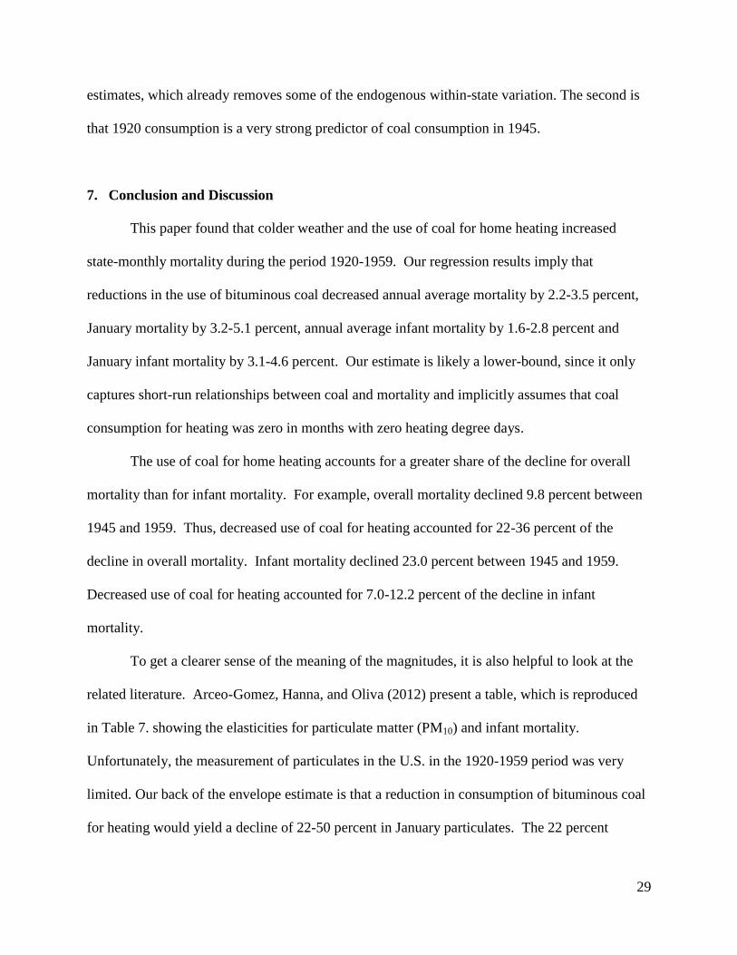
7. Conclusion and Discussion

This paper found that colder weather and the use of coal for home heating increased

state-monthly mortality during the period 1920-1959. Our regression results imply that

reductions in the use of bituminous coal decreased annual average mortality by 2.2-3.5 percent,

January mortality by 3.2-5.1 percent, annual average infant mortality by 1.6-2.8 percent and

January infant mortality by 3.1-4.6 percent. Our estimate is likely a lower-bound, since it only

captures short-run relationships between coal and mortality and implicitly assumes that coal

consumption for heating was zero in months with zero heating degree days.

The use of coal for home heating accounts for a greater share of the decline for overall

mortality than for infant mortality. For example, overall mortality declined 9.8 percent between

1945 and 1959. Thus, decreased use of coal for heating accounted for 22-36 percent of the

decline in overall mortality. Infant mortality declined 23.0 percent between 1945 and 1959.

Decreased use of coal for heating accounted for 7.0-12.2 percent of the decline in infant

mortality.

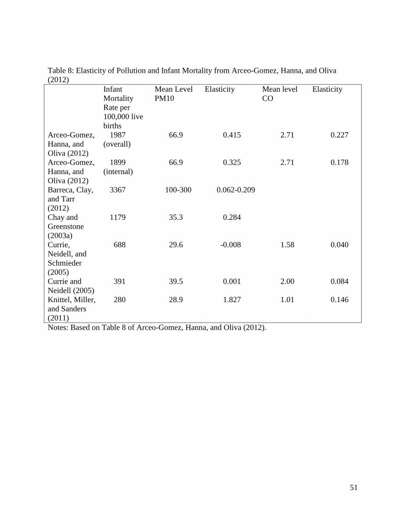
To get a clearer sense of the meaning of the magnitudes, it is also helpful to look at the

related literature. Arceo-Gomez, Hanna, and Oliva (2012) present a table, which is reproduced

in Table 7. showing the elasticities for particulate matter (PM10) and infant mortality.

Unfortunately, the measurement of particulates in the U.S. in the 1920-1959 period was very

limited. Our back of the envelope estimate is that a reduction in consumption of bituminous coal

for heating would yield a decline of 22-50 percent in January particulates. The 22 percent

30

estimate reflects the fact that bituminous coal for heating fell from 22 to 11 percent of

bituminous coal between 1945 and 1959 and assumes that bituminous coal for heating was

burned in half the year. The 50 percent estimate assumes that all of the increase in Figure 4 is

due to the use of coal for heating. The implied elasticity for infant mortality in January is fairly

small relative to contemporary estimates: 0.062-0.209. In comparison, the elasticity for Mexico,

where particulate levels were relatively high, was estimated to be approximately 0.325-0.415.

Our estimates are lower than the two other papers with high levels of PM10 and infant

mortality (Arceo-Gomez et al 2012, Chay and Greenstone 2003a) for at least three reasons. First,

coal consumption, especially for infants, represented a benefit to health from indoor heating.

Other papers use variation in pollution that carried little or no health benefits, such as pollution

from traffic and industrial production. Second, in the U.S. between 1940 and 1959, infant

mortality was high, and interventions for premature or low birth weight babies were extremely

limited. A relatively larger share of babies was dying for other reasons. Third, Chay and

Greenstone (2003a) examines permanent declines in particulates. Their elasticity estimates are

long-run. Our study captures short-run effects and elasticity.

31

Figure 1: Energy Consumption by Source, 1775-2009

Notes: Created from U.S. Energy Administration, History of Energy Consumption in the United States 1775-2009.

http://www.eia.gov/todayinenergy/detail.cfm?id=10

010

20

30

40

Quadri

llio

n B

TU

1750 1800 1850 1900 1950 2000Year

Wood Coal

Natural Gas Petroleum

Hydroelectric Nuclear

32

Figure 2: Coal Consumption by Use

Notes: Values by use are from the Historical Emissions Report and are interpolated for years not ending in 0 or 5.

Non-heating includes bituminous coal used for electricity, industry, coke, and railroads.

0

100

200

300

400

Bit. C

oal in

Millions o

f S

hort

Tons

1920 1930 1940 1950 1960Year

Bituminous Heating Bituminous Non-Heating

33

Figure 3: Seasonality of Retail (Heating) and Other Coal Consumption in 1951

Source: Minerals Yearbook 1952. Other coal consumption includes bituminous coal used for electricity, industry,

coke, and railroads.

11.5

22.5

33.5

Consum

ption R

ela

tive to Y

earl

y M

inim

um

0 3 6 9 12Month

1951 Relative Heating 1951 Relative Other

34

Figure 4: Seasonality of Air Quality in 10 U.S. Cities, 1931-1933

Notes: Ives et al (1936), p. 31. Figure 9: Average atmospheric pollution in American cities for different months of

the year for 1931 to 1933, as determined with the Owens automatic air filter. TSP was also sampled, although with

lower frequency. It was highly correlated with the shade of the Owens automatic air filter. Average TSP in the

winter months in these cities was 510.

35

Figure 5: Real Income and Space Heat per Resident

Source: Strout 1961, Table 1.

35

40

45

50

55

60

BT

Us p

er

capita

1000

1200

1400

1600

1800

Real In

com

e P

er

Capita in 1

954$

1935 1940 1945 1950 1955 1960Year

Real Income Per Capita in 1954$ BTUs per capita

36

Figure 6: Per Capita Consumption of Coal for Heating

Notes: Values for bituminous and anthracite are from the Historical Emissions Report and are interpolated for years

not ending in 0 or 5. National population values are from the Decennial Censuses and are interpolated for years not

ending in 0. Retail (as opposed to sales for electricity, industry, coke, and railroads) sales of anthracite coal are not

available until the 1950s. At that point, they were 20 percent of retail coal sales on a tonnage basis (Minerals

Yearbook). Estimates in the mid 1920s suggested that 65 percent of anthracite was being used for heating.

Department of Commerce (1929), p. 6. The series in Figure 6 uses this 65 percent estimate.

0.2

.4.6

.81

Per

Capita C

oal in

Short

Tons

1910 1920 1930 1940 1950 1960Year

Per Capita Bituminous Per Capita Anthracite

37

Figure 7: Household Heating Fuels in 1940, 1950, and 1960

Source: 1940, 1950, 1960 Censuses of Housing.

Notes: For 1940, Table 60, p. 101 available at

http://www2.census.gov/prod2/decennial/documents/36911485v2p1ch1.pdf . For 1950, Table 20, pp. 127-130

available at http://www2.census.gov/prod2/decennial/documents/36965082v1p1ch1.pdf . For 1960, Table 7, pp. 1-

29-1-33 available at: http://www2.census.gov/prod2/decennial/documents/41962442v1p1ch04.pdf . Other includes

households with electrical (baseboard) heat and no heat.

0.2

.4.6

Share

of H

H u

sin

g F

uel

1940 1950 1960

Coal Wood

Gas Fuel Oil

Other

38

Figure 8: Coal Fields of the United States

Notes: From Fourteenth Census of the United States, Volume XI Mines and Quarries, 1919, General Report and Analytical Tables and Selected Industries, p.

254. http://www2.census.gov/prod2/decennial/documents/23010460v11ch4.pdf

39

Figure 9: Quartile of Per Capita Bituminous Consumption for Heating in 1920

Notes: States were grouped into quartiles, with the shading ranges from lightest (Q1) to darkest (Q4).

40

Figure 10: December Price of Bituminous Coal, Anthracite Coal, and Gas

Source: Historical Statistics of the American Gas Association, Table 231, p. 3

Notes: Prices are in cents per million BTU. The following 20 cities are in the sample: Atlanta, Baltimore, Boston,

Chicago, Cincinnati, Cleveland, Detroit, Houston, Kansas City, Los Angeles, Minneapolis, New York, Philadelphia,

Pittsburgh, Portland, San Francisco, Scranton, Seattle, St. Louis, Washington DC.

41

Figure 11: Gas Heating Equipment Sales, in Thousands of Units

Notes: Historical Statistics of the American Gas Association, Table 143, p. 239

42

Figure 12: Natural Gas Pipelines in 1940 and 1949

Notes: 1940 Map: Federal Trade Commission Monograph no. 36 on Natural Gas Pipelines in the

United States. Reproduced in Castaneda (1993) p. 19. 1949 Map: Parsons (1950), p. 165.

43

Table 1: Estimates of Total Suspended Particulates (TSP) Location Time TSP Source

Chicago 1912-1913 760 Eisenbud (1978)

14 Large US Cities 1931-1933, Winter 510 Ives et al (1936)

US Urban Stations 1953-1957 163 U.S. Department of

Health, Education and

Welfare (1958)

US Urban Stations 1960 118 Lave and Seskin (1972)

US National Average 1990 60 Chay and Greenstone

(2003a)

58 Chinese Cities 1980-1993 538 Almond et al (2009)

Worldwide 1999 18% of urban pop > 200 Cohen et al (2004)

44

Table 2: Summary Statistics

Year Overall Death

Rate per

100,000

Infant Death

Rate per

100,000

Live Births

Per Capita

Bit Coal

Consumption

for Heating in

Tons

Real Income

per capita in

2010 dollars

Heating

Degree Days

relative to 65F

January

Heating

Degree Days

relative to 65F

1920 107.7

(31.7)

0.84

(0.71)

15.8

(14.7)

37.6

(13.0)

1940 88.7

(14.0)

4844.02

(1636.38)

0.67

(0.53)

8,592

(3282)

15.3

(15.0)

41.4

(11.3)

1959 77.7

(10.5)

2673.31

(571.73)

0.18

(0.19)

15,437

(2973)

14.5

(14.1)

34.5

(11.7)

45

Table 3: Overall Mortality, 1920-1959

(1) (2) (3) (4) (5) (6) (7) (8)

LnOverall LnOverall LnOverall LnOverall LnOverall LnOverall LnOverall LnOverall

Monthly Monthly Monthly Monthly Quarterly Quarterly Quarterly Quarterly

HDD 65 0.0050*** 0.0052*** 0.0051*** 0.0047*** 0.0060*** 0.0065*** 0.0062*** 0.0058***

(0.001) (0.001) (0.001) (0.001) (0.001) (0.001) (0.001) (0.001)

Monthly pc bit 508.8412*** 531.1250***

(141.006) (145.203)

Annual pc bit 47.6677*** 39.0024*** 47.9735*** 34.4373**

(14.024) (13.678) (14.026) (13.887)

HDD 65 x 0.5174** 0.8106***

Annual (0.247) (0.284)

pc bit

Year-month

FE Y Y Y Y Y Y Y Y

State-month

FE Y Y Y Y Y Y Y Y

State time

trend Y Y Y Y Y Y Y Y

Observations 21,948 21,948 21,948 21,948 7,316 7,316 7,316 7,316

R-squared 0.883 0.885 0.885 0.885 0.907 0.909 0.909 0.909 Notes: Standard errors are in parentheses and are clustered at the state level. ***, **, and * denote statistical significance at the 1, 5, and 10 percent levels. All

regressions are population weighted. A constant is estimated but not reported. Monthly and annual pc bituminous is measured in 1000s of tons, so a decline of

one ton would be 0.001.

46

Table 4: Infant and Overall Mortality 1940-1959

(1) (2) (3) (4) (5) (6) (7) (8)

LnInfant LnOverall LnInfant LnOverall LnInfant LnOverall LnInfant LnOverall

Monthly Monthly Monthly Monthly Quarterly Quarterly Quarterly Quarterly

HDD 65 0.0044*** 0.0054*** 0.0038*** 0.0051*** 0.0076*** 0.0073*** 0.0068*** 0.0068***

(0.001) (0.001) (0.001) (0.001) (0.001) (0.001) (0.001) (0.001)

Monthly pc bit 442.71*** 364.35** 461.51*** 407.95**

(153.563) (154.237) (160.419) (166.433)

Annual pc bit 5.1990 29.2692 -1.8204 24.2784

(22.536) (20.231) (22.704) (20.287)

HDD 65 x 1.0653*** 0.4655** 1.5651*** 0.8087***

Annual (0.392) (0.196) (0.499) (0.239)

pc bit

Year-month FE Y Y Y Y Y Y Y Y

State-month FE Y Y Y Y Y Y Y Y

State time trend Y Y Y Y Y Y Y Y

Observations 11,640 11,640 11,640 11,640 3,880 3,880 3,880 3,880

R-squared 0.879 0.910 0.879 0.910 0.935 0.938 0.935 0.938 Notes: Standard errors are in parentheses and are clustered at the state level. ***, **, and * denote statistical significance at the 1, 5, and 10 percent levels. All

regressions are population weighted. A constant is estimated but not reported. Monthly and annual pc bituminous is measured in 1000s of tons, so a decline of

one ton would be 0.001.

47

Table 5: Alternative Specifications

(1) (2) (3) (4) (5) (7) (6) (8)

LnOverall LnInfant LnOverall LnInfant LnOverall LnInfant LnOverall LnInfant

Monthly Monthly Monthly Monthly Quarterly Quarterly Quarterly Quarterly

Years 1920-1959 1940-1959 1929-1959 1940-1959 1920-1959 1940-1959 1929-1959 1940-1959

HDD 50 0.0042*** 0.0028**

0.0043*** 0.0058***

(0.001) (0.001)

(0.001) (0.001)

PC Bit 44.282*** 14.3252 12.2811 4.8747 40.544*** 10.5622 2.4543 -4.9982

Heating (13.609) (20.983) (19.705) (23.327) (13.898) (21.525) (20.235) (23.695)

HDD 50 x PC 0.5394* 1.1351**

1.0201** 1.8662***

Bit (0.315) (0.429)

(0.399) (0.662)

HDD 65 -0.0094* 0.0099 -0.0213*** -0.0084

(0.005) (0.012) (0.007) (0.015)

HDD 65 x PC 0.5434* 1.0605** 1.0481*** 1.6031***

Bit (0.317) (0.416) (0.377) (0.546)

PC Bit Non- 37.231*** 10.2209 33.567*** 4.6698

heating (9.761) (15.267) (9.866) (15.542)

HDD 65 x PC 0.1728 -0.0670 0.3133* 0.1052

Bit Non-Heat (0.126) (0.190) (0.161) (0.248)

Ln(pc real -0.0678 0.0444 -0.0838* 0.0165

income) (0.048) (0.052) (0.048) (0.055)

HDD 65 x 0.0014*** -0.0006 0.0027*** 0.0016

Ln(pc inc) (0.001) (0.001) (0.001) (0.002)

Year-month FE Y Y Y Y Y Y Y Y

State-month FE Y Y Y Y Y Y Y Y

State time trend Y Y Y Y Y Y Y Y

Observations 21,360 11,640 17,280 11,640 7,120 3,880 5,760 3,880

R-squared 0.883 0.879 0.886 0.879 0.908 0.935 0.913 0.935 Notes: Standard errors are in parentheses and are clustered at the state level. ***, **, and * denote statistical significance at the 1, 5, and 10 percent levels. All

regressions are population weighted. A constant is estimated but not reported. Monthly and annual pc bituminous is measured in 1000s of tons, so a decline of

one ton would be 0.001.

48

Table 6: Mortality Controlling for Bituminous Coal Consumption in 1920

(1) (2) (3) (4) (5) (6)

LnOverall LnInfant LnOverall LnInfant LnOverall LnInfant

Years 1920-1959 1940-1959 1920-1959 1940-1959 1920-1959 1940-1959

HDD 65 0.0070*** 0.0069*** 0.0023* 0.0017* 0.0046*** 0.0055***

(0.001) (0.001) (0.001) (0.001) (0.002) (0.001)

Coal 1920 x -2.8592*** -3.9956*** -2.2971*** -3.6242***

HDD 65 (0.744) (0.905) (0.708) (0.880)

Coal 1920 x -0.0029*** -0.0079*** -0.0004 -0.0053**

HDD Time (0.001) (0.002) (0.001) (0.003)

Coal 1920 x

HDD Time -0.0027* -0.0036* -0.0019 -0.0026

(post 1945) (0.001) (0.002) (0.002) (0.002)

HDD Time

-0.0000*** -0.0000*** -0.0000** -0.0000

(0.000) (0.000) (0.000) (0.000)

HDD Time

-0.0000 -0.0000 -0.0000 -0.0000

(post 1945)

(0.000) (0.000) (0.000) (0.000)

Year-month FE Y Y Y Y Y Y

State-month FE Y Y Y Y Y Y

State time trend Y Y Y Y Y Y

Observations 21,240 11,520 21,240 11,520 21,240 11,520

R-squared 0.884 0.880 0.884 0.880 0.885 0.880 Notes: Standard errors are in parentheses and are clustered at the state level. ***, **, and * denote statistical significance at the 1, 5, and 10 percent levels. All

regressions are population weighted. Monthly and annual pc bituminous is measured in 1000s of tons, so a decline of one ton would be 0.001.

49

Table 7a: IV using 1945 and 1959

(1) (2) (3) (4)

DLnInfant DLnInfant DLnInfant DLnInfant

OLS OLS IV IV

DHDD65 -0.0025* -0.0027* -0.0023* -0.0027*

(0.001) (0.001) (0.001) (0.001)

DPC Bit -26.2804 -14.0477

(33.478) (35.326)

DPC Bit x 1.4623*** 1.6442*** 1.3359*** 1.6283***

HDD65 (0.244) (0.224) (0.311) (0.253)

State FE N Y N Y

Observations 576 576 576 576

R-squared 0.017 0.468 0.015 0.038

F-Statistic 63.38 181.23

(6) (5) (8) (7)

DLnOverall DLnOverall DLnOverall DLnOverall

OLS OLS IV IV

DHDD65 0.0071*** 0.0056*** 0.0070*** 0.0056***

(0.001) (0.001) (0.001) (0.001)

DPC Bit -0.6953 -2.0751

(14.497) (15.120)

DPC Bit x 1.4912*** 1.3977*** 1.5754*** 1.4641***

HDD65 (0.343) (0.319) (0.335) (0.301)

State FE N Y N Y

Observations 576 576 576 576

R-squared 0.212 0.702 0.212 0.301

F-Statistic 63.38 181.23 Notes: State-month observations were differenced to get the D-variables. Standard errors are in parentheses and are

clustered at the state level. ***, **, and * denote statistical significance at the 1, 5, and 10 percent levels. All

regressions are population weighted. A constant is estimated but not reported. The F-statistic is from the first-stage

regression.

50

Table 7b: IV using 1945 and 1959, First Stage

(1) (2) (3)

DPC Bit DPC Bit x

HDD 65

DPC Bit x

HDD 65

First Stage First Stage First Stage

DHDD65 0.0000 0.0003*** 0.0003***

(0.0000) (0.0001) (0.0001)

Coal 1920 1.052*** 0.0595

(0.091) (0.5611))

Coal 1920 x 0.0009 1.008*** 1.030***

HDD65 (0.0005) (0.0779) (0.0765)

State FE N N Y

Observations 576 576 576

F-statistics 72.89 90.05 181.23

51

Table 8: Elasticity of Pollution and Infant Mortality from Arceo-Gomez, Hanna, and Oliva

(2012)

Infant

Mortality

Rate per

100,000 live

births

Mean Level

PM10

Elasticity Mean level

CO

Elasticity

Arceo-Gomez,

Hanna, and

Oliva (2012)

1987

(overall)

66.9 0.415 2.71 0.227

Arceo-Gomez,

Hanna, and

Oliva (2012)

1899

(internal)

66.9 0.325 2.71 0.178

Barreca, Clay,

and Tarr

(2012)

3367

100-300 0.062-0.209

Chay and

Greenstone

(2003a)

1179 35.3 0.284

Currie,

Neidell, and

Schmieder

(2005)

688 29.6 -0.008 1.58 0.040

Currie and

Neidell (2005)

391 39.5 0.001 2.00 0.084

Knittel, Miller,

and Sanders

(2011)

280 28.9 1.827 1.01 0.146

Notes: Based on Table 8 of Arceo-Gomez, Hanna, and Oliva (2012).

52

References

Almond, Douglas, Yuyu Chen, Michael Greenstone, and Hongbin Li. 2009. "Winter Heating or

Clean Air? Unintended Impacts of China's Huai River Policy." American Economic Review,

99(2): 184–90.

American Gas Association, Bureau of Statistics. Historical Statistics of the Gas Industry. 1956.

Analitis, A. et al. 2008. “Effects of Cold Weather on Mortality: Results from 15 European

Cities Within the PHEWE Project.” American Journal of Epidemiology. 168:1397-1408.

Anderson, Brooke and Michelle Bell. 2009. “How Heat, Cold, and Heat Waves Affect Mortality

in the United States.” Epidemiology 20:205-213.

Arceo-Gomez, Eva, Rema Hanna, and Paulina Oliva. 2012. “Does the Effect of Pollution on

Infant Mortality Differ Between Developing and Developed Countries? Evidence from Mexico

City.” NBER Working Paper #18349.

Butcher Samuel and Michael. Ellenbecker. 1982. “Particulate Emission Factors for Small Wood

and Coal Stoves.” Journal of the Air Pollution Control Association 32:380-384.

Castaneda, Christopher. 1993. Regulated Enterprise: Natural Gas Pipelines and Northeastern

Markets, 1938-1954. Columbus: Ohio State University Press.

Castaneda, Christopher. 1999. Invisible fuel: Manufactured and natural gas in America, 1800-

2000. New York: Twayne.

Chay, Kenneth Y. and Michael Greenstone. 2003a. The Impact of Air Pollution on Infant

Mortality: Evidence from Geographic Variation in Pollution Shocks Induced by a Recession.

Quarterly Journal of Economics, 118: 1121-1167.

Chay, Kenneth Y. and Michael Greenstone. 2003b. Air Quality, Infant Mortality, and the Clean

Air Act of 1970. MIT Department of Economics Working Paper No. 04-08.

Clancy L, Goodman P, Sinclair H, Dockery DW. 2002. Effect of air-pollution control on death

rates in Dublin, Ireland: an intervention study. Lancet 360:1210–1214.

Clay, Karen and Werner Troesken. 2010. “Smoke and the Rise and Fall of the London Fog” in

Climate Change Past and Present. Edited by Gary Libecap and Richard H. Steckel. Chicago:

University of Chicago Press, 2010.

Cohen, Aaron et al. 2004. “Chapter 17: Urban Air Pollution” in Comparative Quantification of

Health Risks, Volume 2. Geneva: World Health Organization.

Currie, Janet and Matthew Neidell. 2005. Air Pollution and Infant Health: What Can We Learn

From California's Recent Experience? Quarterly Journal of Economics 120: 1003-1030.

53

Currie, Janet, Matthew Neidess, Johannes Schmieder. 2009. “Air Pollution and Infant Health:

Lessons from New Jersey.” Journal of Health Economics. 28: 688-703.

Currie, Jarnet and Reed Walker 2011. “Traffic Congestion and Infant Health: Evidence from E-

ZPass.” American Economic Journal: Applied Economics 3:65-90.

Davidson, C.I., and D.L. Davis, “A Chronology of Airborne Particulate Matter in Pittsburgh,” in

History and Reviews of Aerosol Science, G.J. Sem, D. Boulard, P. Brimblecombe, D.S. Ensor,

J.W. Gentry, J.C.M. Marijnissen, and O. Preining, editors, American Association for Aerosol

Research, 2005, pages 347-370.

Delfino, RJ, S Constantinos, and S Malik. 2005. Potential Role of Ultrafine Particles in

Associations between Airborne Particle Mass and Cardiovascular Health. Environmental Health

Perspectives. 113:934-946.

Department of Commerce, Bureau of the Census. 1929. Record Book of Business Statistics. Part

III, Fuels Automobiles, and Rubber. Washington: Government Printing Office.

Eisenbud, Merril. 1978. Levels of Exposure to Sulfur Oxides and Particulates in New York City

and their Sources. Bulletin of the New York Academy of Medicine 1978, 54:991-1011.

Fourteenth Census of the United States, Volume XI Mines and Quarries, 1919, General Report

and Analytical Tables and Selected Industries. Washington: Government Printing Office.

Greensburgh (PA) Daily Tribune, March 22, 1946, p. 1.

Hedley AJ, Wong CM, Thach TQ, Ma S, Lam TH, Anderson HR. 2002. Cardiorespiratory and

all-cause mortality after restrictions on sulphur content of fuel in Hong Kong: an intervention

study. Lancet 360:1646–1652.

Herbert, John H. 1992. Clean Cheap Heat: The Development Of Residential Markets For

Natural Gas In The United States. New York: Greenwood.

Husar, RB and DE Patterson. 1980 Regional Scale Air Pollution: Sources and Effects. Annals of

the New York Academy of Sciences 338: 399-417.

Ives, James et al. 1936. Atmospheric Pollution of American Cities for the Years 1931 to 1933

with Special Reference to the Solid Constituents of the Pollution. U.S. Treasury Department,

Public Health Bulletin No 224. Washington: Government Printing Office.

Junninen, Heikki. 2009. “Quantifying the Impact of Residential Heating on the Urban Air

Quality in a Typical European Coal Combustion Regions.” Environmental Science and

Technology 43: 7964-7970.

Knittel, Christopher, Douglas Miller and Nicholas Sanders. 2011. “Caution, Drivers! Children

Present. Traffic, Pollution and Infant Health.” NBER Working Paper #17222.

54

Laden F, Schwartz J, Speizer FE, Dockery DW. 2006. Reduction in fine particulate air pollution

and mortality: extended follow-up of the Harvard six cities study. Am J Respir Crit Care Med

173(6):581–582.

Lave, Lester and Eugene Seskin. 1972. “Air Pollution, Climate, and Home Heating: Their

Effects on U.S. Mortality Rates.” American Journal of Public Health 62: 909-916.

Lave, Lester and Eugene Seskin. 1977. Air Pollution and Human Health. Baltimore: Johns

Hopkins University Press.

Lesher, C. E. 1917. “Coal in 1917.” U.S. Geological Survey. Part B. Mineral Resources of the

United States. Part II, pp. 1908-1956.

Lockwood, Alan H. 2012. The Silent Epidemic: Coal and the Hidden Threat to Health.

Cambridge: MIT Press.

Minerals Yearbook, various years. U.S. Government Printing Office.

New York Times, various years.

Parsons, James J. 1950. “The Geography of Natural Gas in the United States” Economic

Geography 26: 162-178.

Pope CA III, Schwartz J, Ransom MR. 1992. Daily mortality and PM10 pollution in the Utah

Valley. Arch Environ Health. 47:211–217.

Pope, C. Arden, III, Burnett RT, Thun MJ, Calle EE, Krewski D, Ito K, et al. 2002, “Lung

cancer, cardiopulmonary mortality, and long-term exposure to fine particulate air pollution.”

Journal of the American Medical Association. 287:1132–1141.

Pope CA III, Burnett RT, Thurston GD, Thun MJ, Calle EE,Krewski D, et al. 2004.

Cardiovascular mortality and longterm exposure to particulate air pollution: epidemiological

evidence of general pathophysiological pathways of disease. Circulation 109:71–77.

Pope , C. Arden III. 2007. “Mortality Effects of Longer Term Exposures to Fine Particulate Air

Pollution: Review of Recent Epidemiological Evidence.” Inhalation Toxicology 19: 33-38.

Pope, C. Arden, III, Douglas L. Rodermund, and Matthew M. Gee. 2007. “Mortality Effects of a

Copper Smelter Strike and Reduced Ambient Sulfate Particulate Matter Air Pollution.”

Environmental Health Perspectives. 115(5): 679–683.

Pope, C. Arden, III, Majid Ezzati, Douglas Dockery. 2009. Fine-Particulate Air Pollution and

Life Expectancy in the United States. New England Journal of Medicine 360:376-386.

Powell, Steven. 2009. “Particulate Matter in the Air and its Origins in Coal-Burning Regions.”

Environmental Science and Technology 43: 8474-8474.

55

Schwartz, Joel. 2000. Harvesting and Long Term Exposure Effects in the Relations between Air

Pollution and Mortality. American Journal of Epidemiology, 151: 440-448.

Statistical Abstract of the United States. 1951. Washington: Government Printing Office.

Strout, Alan. 1961. Weather and the Demand for Space Heat. Review of Economics and

Statistics. 43: 185-192.

Tarr, Joel and Karen Clay. 2012. “Pittsburgh as an Energy Capital: Perspectives on Coal and

Natural Gas Transitions and the Environment.” Forthcoming in Energy Capitals: Local Impact,

Global Influence Edited by Martin Melosi and Joseph Pratt. Pittsburgh: University of Pittsburgh

Press.

Tarr, Joel. The Search for the Ultimate Sink: Urban Pollution in Historical Perspective. Akron:

University of Akron Press, 1996.

Tryon, F. G. and H. O. Rogers. 1927. “Consumption of bituminous coal”. U.S. Geological

Survey, Mineral Resources of the United States. Part II, pp. 1908-1956.

U. S. Bureau of the Census. 1889. Census of Manufacturing. Washington: U.S. Government

Printing Office.

U. S. Bureau of the Mines. 1957. Distribution of bituminous coal and lignite shipments. U.S.

Depart of the Interior. Washington: Government Printing Office.

U. S. Bureau of Statistics. 1917. Statistics of Railways in the United States. Interstate

Commerce Commission, Washington DC.

U.S. Department of Health, Education and Welfare 1958. Air Pollution Measurements of the

National Air Sampling Network: Analyses of Suspended Particulates, 1953-1957. Public Health

Service Publication No 637. Washington: Government Printing Office.

Vital Statistics of the United States, various years. Washington: U.S. Government Printing

Office.

Wall Street Journal, various years.

Woodruff, Tracey, Lyndsey Darrow, and Jennifer Parker. 2008. “Air Pollution and Postneonatal

Infant Mortality in the United States, 1999-2002.” Environmental Health Perspectives 116: 110-

115.

Wright, Lawrence. 1964. Home Fires Burning: The History of Domestic Heating and Cooking.

Routledge and Paul.