coastal engineering - unimasr€¦ · 1 waves knowledge of waves and he forces they generate are...
TRANSCRIPT

Coastal Engineering
Prof. K. A. Rakha
Cairo University
Faculty of Engineering
2013

Table of Contents
1 Waves ...................................................................................................... 1-1
1.1 Description of Waves ........................................................................................ 1-1
1.2 Wind and Waves ............................................................................................... 1-2
1.3 Sea and Swell ..................................................................................................... 1-4
1.4 Small Amplitude Wave Theory ....................................................................... 1-5
1.4.1 Solving the Dispersion Equation .................................................................. 1-10
1.5 Reflected Waves .............................................................................................. 1-15
1.6 Short Term Wave Analysis ............................................................................ 1-16
1.6.1 Time Domain Analysis ................................................................................. 1-16
1.6.2 Short-Term Wave Height Distribution ......................................................... 1-17
1.6.3 Frequency Domain Analysis ........................................................................ 1-18
1.7 Wave Generation ............................................................................................ 1-20
1.7.1 Wave Hindcasting ......................................................................................... 1-21
1.8 Wave Transformation .................................................................................... 1-23
1.8.1 Refraction and Shoaling ............................................................................... 1-24
1.8.2 Wave Diffraction. ......................................................................................... 1-27
1.8.3 Wave Breaking ............................................................................................. 1-29
1.9 Wave Models ................................................................................................... 1-33
2 Water Level Variations ......................................................................... 2-1
2.1 Astronomic Tides .............................................................................................. 2-1
2.1.1 Equilibrium Tide (Moon) ............................................................................... 2-2
2.1.2 Daily Inequality .............................................................................................. 2-5
2.1.3 Spring/Neap Tides .......................................................................................... 2-8
2.1.4 Other Effects ................................................................................................. 2-10
2.1.5 Tide Analysis and Prediction ........................................................................ 2-10

K.A.Rakha Jan. 2013 2
2.1.6 Datums .......................................................................................................... 2-13
2.2 Storm Surge..................................................................................................... 2-14
2.3 Barometric Surge ............................................................................................ 2-15
2.4 Seiche ............................................................................................................... 2-17
2.5 Tsunami ........................................................................................................... 2-18
2.6 Eustatic (Sea) Level Change .......................................................................... 2-18
2.7 Isostatic (Land) Rebound and Subsidence ................................................... 2-18
2.8 Global Climate Change .................................................................................. 2-20
3 Currents in the Marine Environment ................................................. 3-1
3.1 Tidal Currents................................................................................................... 3-1
3.2 Wind Generated Currents ............................................................................... 3-1
3.3 Stratification and Density Currents ................................................................ 3-1
3.4 Wave Induced Currents ................................................................................... 3-2
3.4.1 Shore-normal currents .................................................................................... 3-2
3.4.2 Shore-parallel currents .................................................................................... 3-2
3.4.3 Two-dimensional Currents ............................................................................. 3-6
3.5 Hydrodynamic Models ..................................................................................... 3-8
4 Nearshore Sediment Transport ............................................................ 4-1
4.1 Longshore Sediment Transport ...................................................................... 4-3
4.1.1 Predicting Potential Littoral Drift ................................................................... 4-3
4.1.2 Littoral Drift Budget ....................................................................................... 4-4
4.2 On/Offshore Sediment Transport ................................................................... 4-6
4.3 Coastal Sediment Cells ..................................................................................... 4-7
4.4 Sediment Transport Models ............................................................................ 4-8
4.4.1 Morphology and Shoreline Change Models ................................................. 4-10
4.5 One-line Models .............................................................................................. 4-10

K.A.Rakha Jan. 2013 3
4.5.1 Analytical Solution ....................................................................................... 4-12
4.5.2 Model Classification according to Time and Space ..................................... 4-15
4.5.3 Reducing Uncertainty ................................................................................... 4-17
5 References ................................................................................................. 1

1 Waves
Knowledge of waves and he forces they generate are essential for the design of coastal
projects since they are the major factor that determines the geometr of beaches, the
planning and design of marinas, waterways, shore protection measures, hydraulic
structures, and other coastal works.
1.1 Description of Waves
The subject of water waves covers phenomena ranging from capillary waves that have very
short wave periods (order 0.1 seconds) to tides, tsunamis (earthquake generated waves) and
seiches (basin oscillations), where wave periods are expressed in minutes or hours
(Kamphuis, 2000). Wave heights also vary in height from a few millimeters for capillary
waves to 10’s of meters for long waves. A classification by wave frequency of the various
types of waves is given in Fig. 1.1. In the middle of the range of frequencies are the waves
that are the focus of this chapter. They are normally known as gravity waves or wind-
generated waves. Their periods range from 1 to 20 (to 30) seconds and their wave heights
are seldom greater than 10 m. Yet, because of their prevalence, these waves account for
most of the total available wave energy.
Mangor (2004) divides waves into short waves and long waves with short waves of periods
less than 20 second. Long waves are defined as the waves with periods ranging from 20 sec
to 40 min and are divided into surf-beats, harbour resonance, seiche and tsunamis. Water
level oscillations with periods or recurrence intervals larger than an hour such as
astronomical tides and storm surge are referred to as water-level variations.
The shape of a water surface subjected to wind is so complex that it almost defies
description. Even when the first puffs of wind impact an otherwise flat water surface the
resulting distortions present non-linearities that make rigorous analysis impossible. When
the first ripples generated by these puffs are subsequently strengthened by the wind and
interact with each other, the stage has been set for what is known as a confused sea. The
waves will continue to grow ever more complex through processes known only to the sea
itself. It is necessary to simplify the confusion and to use these simplified concepts in
design. This chapter will establish a bridge from the confusing and complex sea state to
theoretical expressions that are simple and can be used for most design purposes.

Waves
K.A.Rakha Jan. 2013 1-2
Figure 1.1: Wave Classification by Frequency (after Kinsman, 1965).
1.2 Wind and Waves
For theoretical analysis of wave generation, the reader is referred to more extensive
references on this subject such as Dean and Dalrymple (1991), Dingemans (1997),
Horikawa (1988), Ippen (1966), Kinsman (1965), Sarpkaya and Isaacson (1981), who
discuss various theoretical models at length. In general, it may be said that wind speed and
wave activity are closely related. There are other important variables to consider such as
depth of water, duration of the storm and fetch (the distance over which the wind blows
over the water and generates waves). At this stage only wind is considered and water
depth, wind duration and fetch are assumed to be unlimited. The resulting waves are often
called Fully Developed Sea and these conditions are approximated only in the deep, open
sea.
The relationship between wind and waves in the open sea is so predictable that sailors have
for centuries drawn a close parallel between wind and waves. The Beaufort Scale in Table
1.1 is a formalized relationship between sea state and wind speed that can be used to obtain
an estimate of waves in the open sea when wind speed is known.
24 h 12 h 5 min 30 s 1 s 0.1 sPeriod
Wave
band
Primary
disturbing
force
Primary
restoring
force
TranstidalLong-period
InfragravityGravity
Ultragravity Capillary
Storm systems, tsunamis
Sun, Moon
Coriolis forceGravity
Wind
Surface tension
Time (s)
En
ergy
(L2)
24 h 12 h 5 min 30 s 1 s 0.1 s
24 h 12 h 5 min 30 s 1 s 0.1 sPeriod
Wave
band
Primary
disturbing
force
Primary
restoring
force
TranstidalLong-period
InfragravityGravity
Ultragravity Capillary
Storm systems, tsunamis
Sun, Moon
Coriolis forceGravity
Wind
Surface tension
Time (s)
En
ergy
(L2)
24 h 12 h 5 min 30 s 1 s 0.1 s

Waves
K.A.Rakha Jan. 2013 1-3
Table 1.1: Beaufort Scale of Wind And Sea State1)
Beaufort
Wind
Force
Wind
Speed
(knots)2)
Description of
wind Description of Sea
Approx
Hs (m)
ApproxT
(sec)
0 0-1 Calm Sea like a mirror. 0 1
1 1-3 Light airs Ripples are formed. 0.025 2
2 4-6 Light breeze
Small wavelets, still short but more
pronounced; crests have a glassy
appearance, but do not break
0.1 3
3 7-10 Gentle breeze Large wavelets, crests begin to break.
Perhaps scattered white caps. 0.4 4
4 11-21 Moderate
breeze
Small waves, becoming larger; fairly
frequent white capping. 1 5
5 17-21 Fresh breeze
Moderate waves, taking a more
pronounced long form; many white caps
are formed (chance of some spray).
2 6
6 22-27 Strong breeze
Large waves begin to form; the white
foam crests are more extensive
everywhere (probably some spray).
4 8
7 28-33 Moderate gale
Sea heaps up and white foam from
breaking waves begins to be blown in
streaks along the direction of the wind
(spindrift).
7 10
8 34-40 Fresh gale
Moderately high waves of greater length;
edges of crests break into spindrift. The
foam is blown in well-marked streaks
along the direction of the wind. Spray
affects visibility.
11 13
9 41-47 Strong gale
High waves. Dense streaks of foam along
the direction of the wind. Sea begins to
roll. Visibility affected.
18 16
10 48-55 Whole gale3)
Very high waves with long overhanging
crests. The resulting foam is in great
patches and is blown in dense white
streaks along the direction of the wind.
On the whole, the surface of the sea takes
a white appearance. The rolling of the sea
becomes heavy and shocklike. Visibility
is affected.
25 18
11 56-63 Storm3)
Exceptionally high waves (small and
medium sized ships might for a long time
be lost to view behind the waves). The
sea is completely covered with long white
patches of foam lying along the direction
of the wind. Visibility affected.
354) 204)
12 64-71 Hurricane3)
Air filled with foam and spray. Sea
completely white with driving spray;
visibility very seriously affected.
404) 224)
1) Fully developed sea - unlimited fetch and duration. 2) 1 knot 1.8 km/hr 0.5 m/s 3) Required durations and fetches are seldom attained to generate fully developed sea. 4) Really only a 30-40 m deep interface between sea and air.
Waves
K.A.Rakha Jan. 2013 1-4
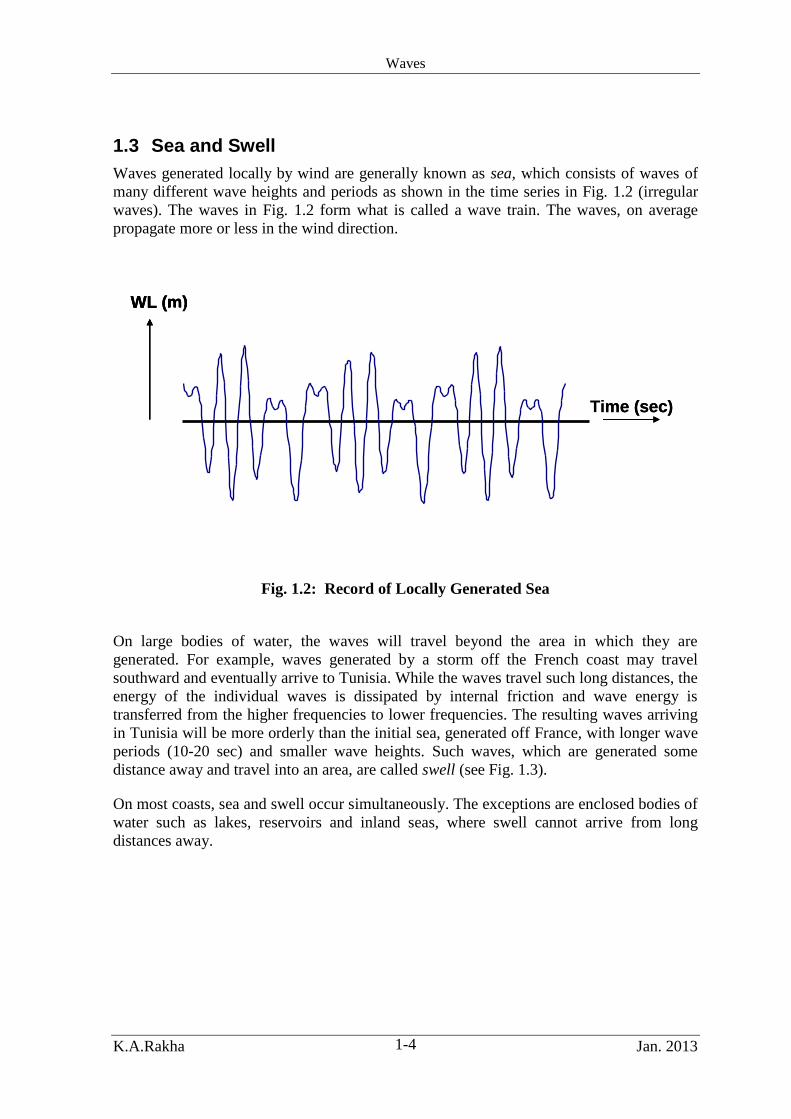
1.3 Sea and Swell
Waves generated locally by wind are generally known as sea, which consists of waves of
many different wave heights and periods as shown in the time series in Fig. 1.2 (irregular
waves). The waves in Fig. 1.2 form what is called a wave train. The waves, on average
propagate more or less in the wind direction.
Fig. 1.2: Record of Locally Generated Sea
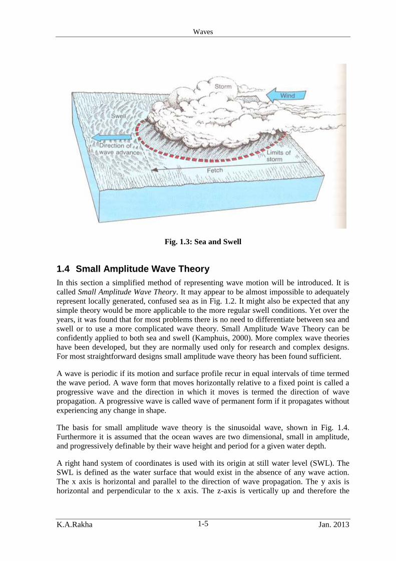
On large bodies of water, the waves will travel beyond the area in which they are
generated. For example, waves generated by a storm off the French coast may travel
southward and eventually arrive to Tunisia. While the waves travel such long distances, the
energy of the individual waves is dissipated by internal friction and wave energy is
transferred from the higher frequencies to lower frequencies. The resulting waves arriving
in Tunisia will be more orderly than the initial sea, generated off France, with longer wave
periods (10-20 sec) and smaller wave heights. Such waves, which are generated some
distance away and travel into an area, are called swell (see Fig. 1.3).
On most coasts, sea and swell occur simultaneously. The exceptions are enclosed bodies of
water such as lakes, reservoirs and inland seas, where swell cannot arrive from long
distances away.
WL (m)
Time (sec)
WL (m)WL (m)
Time (sec)
Waves
K.A.Rakha Jan. 2013 1-5
Fig. 1.3: Sea and Swell
1.4 Small Amplitude Wave Theory
In this section a simplified method of representing wave motion will be introduced. It is
called Small Amplitude Wave Theory. It may appear to be almost impossible to adequately
represent locally generated, confused sea as in Fig. 1.2. It might also be expected that any
simple theory would be more applicable to the more regular swell conditions. Yet over the
years, it was found that for most problems there is no need to differentiate between sea and
swell or to use a more complicated wave theory. Small Amplitude Wave Theory can be
confidently applied to both sea and swell (Kamphuis, 2000). More complex wave theories
have been developed, but they are normally used only for research and complex designs.
For most straightforward designs small amplitude wave theory has been found sufficient.
A wave is periodic if its motion and surface profile recur in equal intervals of time termed
the wave period. A wave form that moves horizontally relative to a fixed point is called a
progressive wave and the direction in which it moves is termed the direction of wave
propagation. A progressive wave is called wave of permanent form if it propagates without
experiencing any change in shape.
The basis for small amplitude wave theory is the sinusoidal wave, shown in Fig. 1.4.
Furthermore it is assumed that the ocean waves are two dimensional, small in amplitude,
and progressively definable by their wave height and period for a given water depth.
A right hand system of coordinates is used with its origin at still water level (SWL). The
SWL is defined as the water surface that would exist in the absence of any wave action.
The x axis is horizontal and parallel to the direction of wave propagation. The y axis is
horizontal and perpendicular to the x axis. The z-axis is vertically up and therefore the

Waves
K.A.Rakha Jan. 2013 1-6
position of the bottom is at z = -d. The highest point of the wave is the crest and the lowest
point is the trough. The sinusoidal water surface η may be described by,
T
t
L
xat) - (kx a =
22coscos (1.1)
where a is the amplitude of the wave, x is distance in the direction of wave propagation, t is
time, k is the wave number (the angular frequency at which the wave pattern repeats itself
in space), is the angular wave frequency (the angular frequency of repetition in time), L
is the wave length and T is the wave period. The values of k and are calculated from,
T
2 =
L
2 = k
; (1.2)
The maximum vertical distance between crest and trough of the wave is called the wave
height, H(=2a). Since in an actual wave train, such as in Fig. 1.2, the wave heights and
lengths are not all the same, statistical representative values are used. The ratio of wave
height to wave length (H/L) is called wave steepness. The wave form moves forward and
the velocity of propagation of the wave (or phase speed) is calculated from,
T
L = C (1. 3)
Mean water level (MWL) is defined as the level midway between wave crest and trough.
In small amplitude wave theory, MWL is the same as SWL, but for higher order wave
theories MWL will be above SWL Further, waves are differentiated as Long-Crested or
Short-Crested which refers to the length of the wave crest perpendicular to the wave shape
and its velocity of propagation. Swell is normally long crested (the wave is recognizable as
a single crest over a hundred meters or so) and Sea is normally short crested. Waves are
considered to be in deep water when d/L > 0.5 and in shallow water when d/L > .0.0.
Between these limiting conditions, the water depth is called transitional.
The Small Amplitude Wave Theory expressions are summarized in Table 1.2. Equation [1]
(equation numbers in square brackets refer to those in Table 1.2) describes the water
surface fluctuation as shown in Fig. 1.4. Equation [2] calculates the velocity of
propagation, C, assuming the wave retains a constant form. The 'tanh' term has two
asymptotic values. For large depths, kd (or d/L) is large resulting in,
1 L
d = kd
2tanhtanh (1.4)
For small depths,
)L
d2( )
L
d2( = kd
tanhtanh (1. 5)
Thus, it is possible to give deep and shallow water asymptotic values for C as in Table 1.2.
It has been customary to define deep water as d/L>0.5 (tanh kd = 0.996) and shallow water
is usually defined as d/L<0.05 (kd = 0.592, while tanh kd = 0.531).

Waves
K.A.Rakha Jan. 2013 1-7
Fig. 1.4: Sinusoidal Wave and Wave Parameters
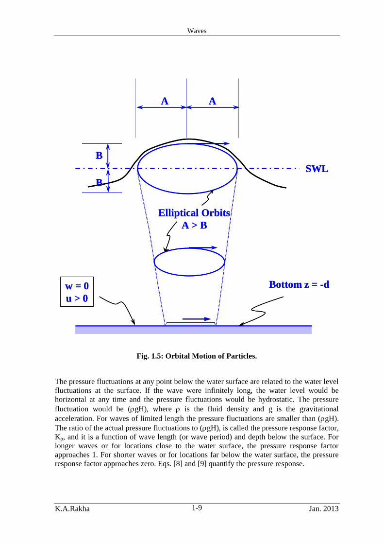
Waves propagate at velocity C, but the individual water particles do not propagate; they
move in particle orbits as shown in Fig. 1.5. For small amplitude wave theory, such particle
orbits are elliptical and if the water is 'deep', they become circular. Their size decreases
with depth. Horizontal and vertical orbital velocity components, u and w, and orbit
semi-axes, A and B, are given in Eqs. [4] to [7].
SWL
L
x
z
c
Ha=H/2
Trough
Crest
d
z = -d
SWL
L
x
z
c
Ha=H/2
Trough
Crest
d
z = -d

Waves
K.A.Rakha Jan. 2013 1-8
Table 1.2: Common Expressions for Linear Progressive Waves
Parameter General Deep
(d/L > 0.5)
Shallow
(d/L < 0.05)
1. Water Surface
t)(kx-
cos 2
H =
w
2. Velocity of
Propagation
(Dispersion
Equation) kd tanh
2
gL =
kd tanh 2
gT =
k =
T
L = C
2
gT = Co gd = C
3. Wave Length kd tanh 2
gT = CT = L
2
2
gT = L
2
o CTL
4. Horizontal
Orbital Velocity w
cos
kdsinh
d)k(z+cosh
T
H =u
wT
cos e H
= uzko
oo
wd
gcos
2
H =u
5. Vertical
Orbital Velocity w
sin kdsinh
d)k(z+sinh
T
H = w
wT
sin e H
= wzko
oo
wd
z
T
sin 1
H = w
6. Horizontal
Semi- Axis kdsinh
d)(z+kcosh
2
H =A e
2
H = A
zkoo
o
4
H = A
d
gT
7. Vertical Semi-
Axis kdsinh
d)(z+ksinh
2
H = B
A = B oo 1
2
H = B
d
z
8. Pressure
Kz+- = g
pp
9. Pressure
Response Factor kdcosh
d)(z+coshk = K p
e = Kzk
po
1 = Kp
10. Energy
Density
2
8
1gHE
11. Wave Power EC = P G
2
EC = P
oo EC = P
12. Group
Velocity Cn = CG
2
C = C
o
G o C = CG
13. Group
Velocity
Parameter
kd2sinh
kd2 + 1
2
1 =n
2
1 = n o 1 =n
Waves
K.A.Rakha Jan. 2013 1-9
Fig. 1.5: Orbital Motion of Particles.
The pressure fluctuations at any point below the water surface are related to the water level
fluctuations at the surface. If the wave were infinitely long, the water level would be
horizontal at any time and the pressure fluctuations would be hydrostatic. The pressure
fluctuation would be (gH), where is the fluid density and g is the gravitational
acceleration. For waves of limited length the pressure fluctuations are smaller than (gH).
The ratio of the actual pressure fluctuations to (gH), is called the pressure response factor,
Kp, and it is a function of wave length (or wave period) and depth below the surface. For
longer waves or for locations close to the water surface, the pressure response factor
approaches 1. For shorter waves or for locations far below the water surface, the pressure
response factor approaches zero. Eqs. [8] and [9] quantify the pressure response.
Elliptical Orbits
A > B
A A
B
B
SWL
Bottom z = -dw = 0
u > 0
Elliptical Orbits
A > B
A A
B
B
SWL
Bottom z = -dw = 0
u > 0

Waves
K.A.Rakha Jan. 2013 1-10
Wave Energy is expressed per unit surface area as Energy Density, E, in joules/m2
as in Eq.
[10]. It is made up of half Potential Energy and half Kinetic Energy. Eq. [11] gives Wave
Power, P, arriving at any location. Its units are watts/m of wave crest.
Eq. [2] indicates that longer period waves travel faster than shorter period waves. A real
wave train, as in Fig. 1.2, contains many different wave periods and therefore it would
stretch out (disperse) as it traveled. The longest waves would lead and run further and
further ahead with time and distance, while the shortest waves would lag further behind.
Hence Eq. [2] is called the Dispersion Equation.
Equation [2] also means that waves of roughly the same period tend to travel together.
Waves of almost the same period interfere to form beats or wave groups, resulting in two
wave speeds involved: the speed of the individual waves given by Eq. [2] and the speed of
the wave group, which is C multiplied by the factor n, given in Eq. [13]. In deep water n
approaches ½ and in shallow water n approaches 1. Thus CG<C, but in very shallow water
CG approaches C.
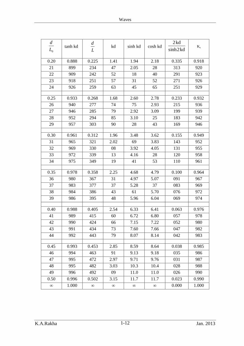
1.4.1 Solving the Dispersion Equation
To solve Eq. [2] and all the other equations in Table 1.2, it is necessary to know the wave
length, L, which may be calculated using Eq. [3]. However, Eq. [3] is implicit and can only
be solved numerically. Tables of solutions have been prepared that yield L as well as other
important wave characteristics (see Table 1.3). Such tables are known as Wave Tables and
have been published in Shore Protection Manual (l984) and Wiegel (l964). To use the
wave tables, the deep water approximation of wave length is first calculated as given by
Eq. [3]. Then using the depth of water, d, it is possible to enter the wave tables with d/Lo to
evaluate all the remaining wave parameters.
The use of the wave table is suitable for only a few calculations. For a large number of
calculations, L or C may be calculated using a root finding technique such as
Newton-Raphson, but such a technique requires iteration. To speed up such computations,
approximations may be used such as the one proposed by Hunt (1979),
)y0.0675 + y0.0864 + y0.4622 +0.6522y + (1 +y = gd
C 1-542 1-2
(1. 6)
where
L
d2 =y
o
(1. 7)

Waves
K.A.Rakha Jan. 2013 1-11
Table 1.3: Wave Table
0L
d tanh kd
L
d kd sinh kd cosh kd
kd2sinh
kd2 Ks
0.000 0.000 0.0000 0.000 0.000 1.00 1.000 ∞
002 112 0179 112 113 01 0.992 2.12
004 158 0253 159 160 01 983 1.79
006 193 0311 195 197 02 975 62
008 222 0360 226 228 03 967 51
0.010 0.248 0.0403 0.253 0.256 1.03 0.958 1.43
015 302 0496 312 317 05 938 31
020 347 0576 362 370 07 918 23
025 386 0648 407 418 08 898 17
0.030 0.420 0.0713 0.448 0.463 1.10 0.878 1.13
035 452 0775 487 506 12 858 09
040 480 0833 523 548 14 838 06
045 507 0888 558 588 16 819 04
0.050 0.531 0.0942 0.592 0.627 1.18 0.800 1.02
055 554 0993 624 665 20 781 1.01
060 575 104 655 703 22 762 0.993
065 595 109 686 741 24 744 981
070 614 114 716 779 27 725 971
0.075 0.632 0.119 0.745 0.816 1.29 0.707 0.962
080 649 123 774 854 31 690 955
085 665 128 803 892 34 672 948
090 681 132 831 929 37 655 942
095 695 137 858 0.968 39 637 937
0.10 0.709 0.141 0.886 1.01 1.42 0.620 0.933
11 735 150 940 08 48 587 926
12 759 158 0.994 17 54 555 920
13 780 167 1.05 25 60 524 917
14 800 175 10 33 67 494 915
0.15 0.818 0.183 1.15 1.42 1.74 0.465 0.913
16 835 192 20 52 82 437 913
17 850 200 26 61 90 410 913
18 864 208 31 72 1.99 384 914
19 877 217 36 82 2.08 359 916
Waves
K.A.Rakha Jan. 2013 1-12
0L
d tanh kd
L
d kd sinh kd cosh kd
kd2sinh
kd2 Ks
0.20 0.888 0.225 1.41 1.94 2.18 0.335 0.918
21 899 234 47 2.05 28 313 920
22 909 242 52 18 40 291 923
23 918 251 57 31 52 271 926
24 926 259 63 45 65 251 929
0.25 0.933 0.268 1.68 2.60 2.78 0.233 0.932
26 940 277 74 75 2.93 215 936
27 946 285 79 2.92 3.09 199 939
28 952 294 85 3.10 25 183 942
29 957 303 90 28 43 169 946
0.30 0.961 0.312 1.96 3.48 3.62 0.155 0.949
31 965 321 2.02 69 3.83 143 952
32 969 330 08 3.92 4.05 131 955
33 972 339 13 4.16 28 120 958
34 975 349 19 41 53 110 961
0.35 0.978 0.358 2.25 4.68 4.79 0.100 0.964
36 980 367 31 4.97 5.07 091 967
37 983 377 37 5.28 37 083 969
38 984 386 43 61 5.70 076 972
39 986 395 48 5.96 6.04 069 974
0.40 0.988 0.405 2.54 6.33 6.41 0.063 0.976
41 989 415 60 6.72 6.80 057 978
42 990 424 66 7.15 7.22 052 980
43 991 434 73 7.60 7.66 047 982
44 992 443 79 8.07 8.14 042 983
0.45 0.993 0.453 2.85 8.59 8.64 0.038 0.985
46 994 463 91 9.13 9.18 035 986
47 995 472 2.97 9.71 9.76 031 987
48 995 482 3.03 10.3 10.4 028 988
49 996 492 09 11.0 11.0 026 990
0.50 0.996 0.502 3.15 11.7 11.7 0.023 0.990
∞ 1.000 ∞ ∞ ∞ ∞ 0.000 1.000

Waves
K.A.Rakha Jan. 2013 1-13
Example 1.1
In this example the small amplitude wave parameters given in Table 1.2 are calculated for
a wave of period, T = 10 sec, with a wave height, H = 1.5 m in a depth of water, d = 9.4 m.
First, it is necessary to calculate the deep water wave length and relative depth:
060.0156
4.9;156)100(56.156.1
2
22
o
oL
dmT
gTL
The wave table (Table 1.3) yields the following:
0.881=n; 1.22kd; 0.703=kd
; 0.575=kd; 0.104=L
d
)762.01(*5.0coshsinh
tanh
From the value of L
d, the wave length in 9.4 m of water and wave number, k, may now be
calculated:
069.02
;4.90104.0
L
kmd
L
From these, the following parameters may be computed; is assumed to be 1035 kg/m3 for
sea water.
crestwaveof w/mECPj/m gH
E
m/s CnCm/s =T
L=C
G
G
730,22;28548
;96.7)04.9(881.0;04.9
2
At the bottom:
0.1)(cosh;0)(sinh;0)(; dzkdzkdzkdz
and the horizontal component of orbital velocity is:
)cos(67.0)cos(703.
1
10
)5.1()cos(
sinh
1tkxtkxtkx
kdT
HuB
Thus, at the bottom, uB has a maximum value uB = 0.67 m/s and the vertical velocity
component of orbital motion at the bottom is zero. The amplitude of the orbital motion at
the bottom is

Waves
K.A.Rakha Jan. 2013 1-14
m. 1.07 = (0.703) 2
1.5 =
kd 2
H = AB
sinh
and the orbital diameter is 2AB = 2.14 m. The pressure response factor Kp at the bottom is:
0.82 = 1.22
1 =
kd = K Bpcosh
1)(
which means that the maximum pressure fluctuation caused by the wave height H = 1.5 m
is:
water)of (m)( 1.23 = 1.50.82 = H K p
Waves
K.A.Rakha Jan. 2013 1-15
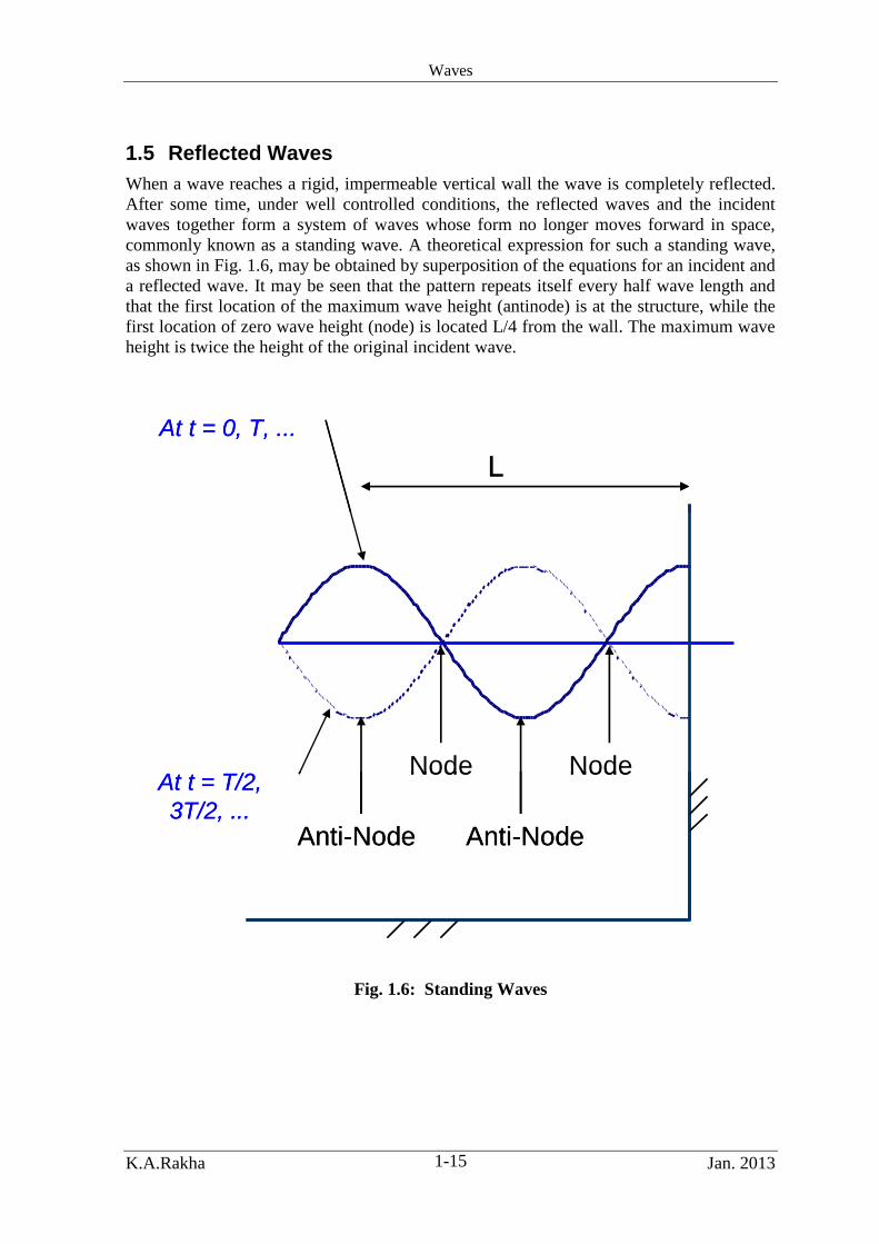
1.5 Reflected Waves
When a wave reaches a rigid, impermeable vertical wall the wave is completely reflected.
After some time, under well controlled conditions, the reflected waves and the incident
waves together form a system of waves whose form no longer moves forward in space,
commonly known as a standing wave. A theoretical expression for such a standing wave,
as shown in Fig. 1.6, may be obtained by superposition of the equations for an incident and
a reflected wave. It may be seen that the pattern repeats itself every half wave length and
that the first location of the maximum wave height (antinode) is at the structure, while the
first location of zero wave height (node) is located L/4 from the wall. The maximum wave
height is twice the height of the original incident wave.
Fig. 1.6: Standing Waves
L
Node Node
Anti-Node Anti-Node
At t = 0, T, ...
At t = T/2,
3T/2, ...
L
Node Node
Anti-Node Anti-Node
At t = 0, T, ...
At t = T/2,
3T/2, ...

Waves
K.A.Rakha Jan. 2013 1-16
Partial wave reflection will result if the reflecting surface is sloping, flexible or porous and
yields a variation in wave height. The partial antinodes (Hmax) are less than twice the
incident wave height, while the partial nodes (Hmin) are greater than zero.
1.6 Short Term Wave Analysis
In the first part of this chapter, waves on the sea surface were assumed to be nearly
sinusoidal with constant height, period and direction (i.e., monochromatic waves). Visual
observation of the sea surface and measurements indicate that the sea surface is composed
of waves of varying heights and periods moving in differing directions. In the first part of
this chapter, wave height, period, and direction could be treated as deterministic quantities.
Once we recognize the fundamental variability of the sea surface, it becomes necessary to
treat the characteristics of the sea surface in statistical terms. This complicates the analysis
but more realistically describes the sea surface. The term irregular waves will be used to
denote natural sea states in which the wave characteristics are expected to have a statistical
variability in contrast to monochromatic waves, where the properties may be assumed
constant. Monochromatic waves may be generated in the laboratory but are rare in nature.
In analysis of wave data, it is important to distinguish between Short-Term and Long-Term
wave analysis. Short-Term analysis refers to analysis of waves that occur within one wave
train or within one storm; Long-Term analysis refers to the derivation of distributions that
cover many years. This section deals with short term wave analysis.
Two approaches exist for short term analysis of irregular waves: spectral methods and
wave-by-wave (wave train) analysis. Spectral approaches are based on the Fourier
Transform of the sea surface. This analysis is usually called frequency domain analysis
since the wave spectra is used rather than a time series. Indeed this is currently the most
mathematically appropriate approach for analyzing a time-dependent, three-dimensional
sea surface record. Unfortunately, it is exceedingly complex and at present few
measurements are available that could fully tap the potential of this method. However,
simplified forms of this approach have been proven to be very useful.
The other approach used is wave-by-wave analysis. In this analysis method, a time-history
of the sea surface at a point is used, the undulations are identified as waves, and statistics
of the record are developed. This method is used called the time domain analysis since it
deals with a time series of the water surface. The primary drawback to the wave-by-wave
analysis is that it cannot tell anything about the direction of the waves. Indeed, what
appears to be a single wave at a point may actually be the local superposition of two
smaller waves from different directions that happen to be intersecting at that time.
Disadvantages of the spectral approach are the fact that it is linear and can distort the
representation of nonlinear waves.
1.6.1 Time Domain Analysis
In the time-domain analysis of irregular or random seas, wave height and period,
wavelength, wave crest, and trough have to be carefully defined for the analysis to be
performed. The definitions provided earlier in the regular wave section of this chapter
assumed that the crest of a wave is any maximum in the wave record, while the trough can
be any minimum. However, these definitions may fail when two crests occur within an

Waves
K.A.Rakha Jan. 2013 1-17
intervening trough lying below the mean water line. Also, there is not a unique definition
for wave period, since it can be taken as the time interval between either two neighbouring
wave troughs or two crests. Other more common definitions of wave period are the time
interval between successive crossings of the mean water level by the water surface in a
downward direction called zero down-crossing period or zero up-crossing period for the
period deduced from successive up-crossings.
Using these definitions of wave parameters for an irregular sea state, the periods and
heights of irregular waves are not constant with time, changing from wave to wave. Wave-
by-wave analysis determines wave properties by finding average statistical quantities (i.e.,
heights and periods) of the individual wave components present in the wave record. Wave
records must be of sufficient length to contain several hundred waves for the calculated
statistics to be reliable.
Average statistical representations for an irregular sea state may be defined in several
ways. These include the mean height H , the root-mean-square height, and the mean height
of the highest one-third of all waves known as the significant height. Among these, the
most commonly used is the significant height, denoted as Hs or H1/3. Significant wave
height has been found to be very similar to the estimated visual height by an experienced
observer (Kinsman, 1965). The average of the highest 10% (H0.1) or the highest 1% (H0.01)
is also sometimes used for design purposes. The average statistical period could be the
mean period, or average zero-crossing period, etc.
1.6.2 Short-Term Wave Height Distribution
The heights of individual waves may be regarded as a stochastic variable represented by a
Probability Distribution Function (PDF). From an observed wave record, such a function
can be obtained from a histogram of wave heights normalized with the mean heights in
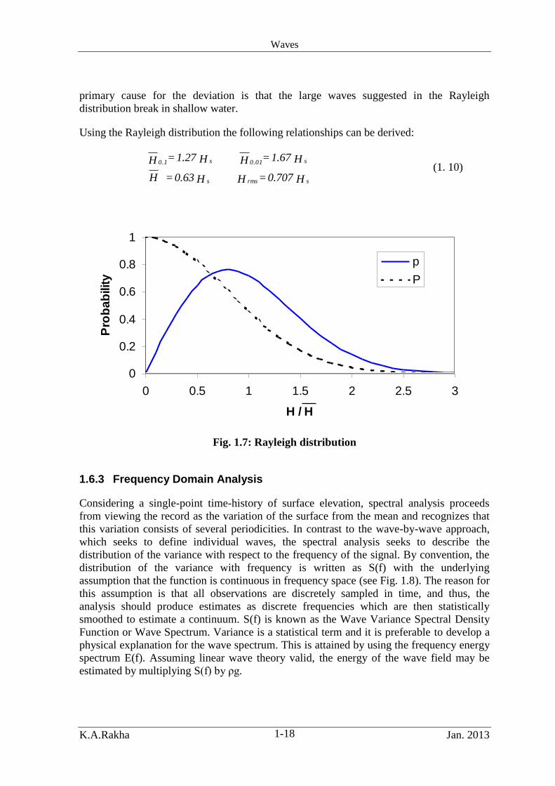
several wave records measured at a point. The Rayleigh distribution was found to be the
most suitable distribution for representing wave heights within a storm (short term). Figure
1.7 shows the Rayleigh distribution (p curve) together with the cumulative Rayleigh
distribution (P curve). Equation (1.8) provides the equation for the Rayleigh PDF,
2
4exp
2 H
H
H
H
H
Hp
(1. 8)
The Cumulative Distribution Function (CDF) of wave heights based on the Rayleigh
distribution (the probability that any individual wave of height H' is not higher than a
specified wave height H) can be written as,
2
4exp
H
H
H
HP
(1. 9)
The Rayleigh distribution is generally adequate, except in shallow water in which it may
overestimate the number of large waves. Investigations of shallow-water wave records
from numerous studies indicate that the distribution deviates from the Rayleigh, and other
distributions have been shown to fit individual observations better (SPM, 1984). The
Waves
K.A.Rakha Jan. 2013 1-18
primary cause for the deviation is that the large waves suggested in the Rayleigh
distribution break in shallow water.
Using the Rayleigh distribution the following relationships can be derived:
H 0.707 = H H 0.63 = H
H 1.67 = H H 1.27 = H
srmss
s0.01s0.1 (1. 10)
Fig. 1.7: Rayleigh distribution
1.6.3 Frequency Domain Analysis
Considering a single-point time-history of surface elevation, spectral analysis proceeds
from viewing the record as the variation of the surface from the mean and recognizes that
this variation consists of several periodicities. In contrast to the wave-by-wave approach,
which seeks to define individual waves, the spectral analysis seeks to describe the
distribution of the variance with respect to the frequency of the signal. By convention, the
distribution of the variance with frequency is written as S(f) with the underlying
assumption that the function is continuous in frequency space (see Fig. 1.8). The reason for
this assumption is that all observations are discretely sampled in time, and thus, the
analysis should produce estimates as discrete frequencies which are then statistically
smoothed to estimate a continuum. S(f) is known as the Wave Variance Spectral Density
Function or Wave Spectrum. Variance is a statistical term and it is preferable to develop a
physical explanation for the wave spectrum. This is attained by using the frequency energy
spectrum E(f). Assuming linear wave theory valid, the energy of the wave field may be
estimated by multiplying S(f) by ρg.
0
0.2
0.4
0.6
0.8
1
0 0.5 1 1.5 2 2.5 3
H / H
Pro
ba
bilit
y
p
P
0
0.2
0.4
0.6
0.8
1
0 0.5 1 1.5 2 2.5 3
H / H
Pro
ba
bilit
y
p
P

Waves
K.A.Rakha Jan. 2013 1-19
The surface can be envisioned not as individual waves but as a three-dimensional surface,
which represents a displacement from the mean and the variance to be periodic in time and
space. The simplest spectral representation is to consider E(f,θ), which represents how the
variance is distributed in frequency f and direction θ. E(f,θ) is called the 2-D or directional
energy spectrum because it can be multiplied by ρg to obtain wave energy. The advantage
of this representation is that it tells the engineer about the direction in which the wave
energy is moving.
The different wave height statistics (e.g. significant wave height) can be determined from
the moments of the wave spectra. The moments of the wave spectrum are defined as,
df S(f) f = mn
0n
f
f (1. 11)
The zero moment is therefore the area under the spectrum
2
0o = df S(f) = m f
f
f
(1. 12)
From the area under the wave spectrum, assuming the wave height distribution to be
Rayleigh, the various wave heights may be estimated. To distinguish between significant
wave height (derived from time domain analysis) and its counterpart, derived from
frequency analysis, the latter is called the Characteristic Wave Height or Zero Moment
Wave Height.
fmoch 4 = H = H (1. 13)
The representation of the wave energy distribution with frequency is a large improvement
over the time-domain analysis methods discussed earlier. With this information it is
possible to study resonant systems such as the response of drilling rigs, ships' moorings,
etc. to wave action, since it is now known in which frequency bands the forcing energy is
concentrated. It is also possible to separate sea (shorter period waves) and swell (longer
period waves) via the wave spectrum, when both occur simultaneously.
Since there are many wave frequencies (or wave periods) represented in the spectrum it is
usual to characterize the wave spectrum by its peak frequency fp, the frequency at which
the spectrum displays its largest variance (or energy). The peak period may be defined as,
f
1 = T
p
p (1. 14)
Since the measured spectra show considerable similarity, a number of attempts have been
made to formulate parametric expressions. One commonly used spectrum in wave
hindcasting and forecasting projects is the single-parameter spectrum of Pierson-
Moskowitz PM (Pierson and Moskowitz 1964). An extension of the PM spectrum is the
JONSWAP spectrum (Hasselmann et al. 1973, 1976).

Waves
K.A.Rakha Jan. 2013 1-20
Fig. 1.8: Wave spectra.
1.7 Wave Generation
When a gentle breeze blows over water, the turbulent eddies in the wind field will
periodically touch down on the water, causing local disturbances of the water surface. The
wind speed must be in excess of 0.23 m/s to overcome the surface tension in the water.
Theory (Phillips, 1957) shows wind energy is transferred to waves most efficiently when
they both travel at the same speed. But wind speed is normally greater than the wave
speed. For this reason the generated waves will form as an angle to the wind direction so
that the component of wind speed in the direction of wave propagation approaches the
wave speed. The generated wave crests are short crested, irregular waves.
Once the initial wavelets have been formed and the wind continues to blow, energy is
transferred from the wind to the waves. Much of the wind energy is transferred to the
higher frequency waves, i.e., the wind causes more ripples to form on top of existing
waves, rather than increasing the size of the larger waves directly by shear and pressure
differences. This pool of high frequency energy is then transferred to lower frequencies by
the interaction of the high frequency movement with the adjacent slower moving water
particles. This wave-wave interaction transfers wave energy to the lower frequencies of the
wave spectrum.
Earlier we stated that wave height and wave period is closely related to wind speed. It
should therefore be possible to derive wave conditions from known wind conditions. In
fact, it should be possible to reconstruct a wave climate at a site from historical, measured
wind records. Such a computation is known as Wave Hindcasting.
f (Hz)fp
S(f)
(m2/Hz)
Area = 2f

Waves
K.A.Rakha Jan. 2013 1-21
1.7.1 Wave Hindcasting
For most locations, it is difficult to find long term wave data that is essential for the design
of any coastal project. Hindcasted wave data is usually used for such purposes.
1.7.1.1 Parametric Methods
The theory of wave generation has had a long and rich history. Beginning with some of the
classic works of Kelvin (1887) and Helmholtz (1888) in the 1800's, many scientists,
engineers, and mathematicians have addressed various forms of water wave motions and
interactions with the wind. In the early 1900's, the work of Jeffreys (1924, 1925)
hypothesized that waves created a "sheltering effect" and hence created a positive feedback
mechanism for transfer of momentum into the wave field from the wind. However, it was
not until World War II that organized wave predictions began in earnest. During the
1940's, large bodies of wave observations were collated and the bases for empirical wave
predictions were formulated. Sverdrup and Munk (1947) presented the first documented
relationships among various wave-generation parameters and resulting wave conditions.
The method was later extended by Bretschneider (e.g., Bretschneider, 1958) to form the
empirical method, now known as the SMB Method. The method is described fully in
Shore Protection Manual (1977). In Shore Protection Manual (1984) this method was
replaced by the Jonswap Method, based on research on wave spectra in growing seas by
Hasselmann et al (1973).
The Jonswap, SMB and similar methods are called parametric methods because they use
wind parameters to produce wave parameters, rather than develop a detailed description of
the physics of the processes. Although, these methods produce only Significant Wave
Height (Hs) and Significant Wave Period (Ts), they may be extended to provide estimates
of the parametric wave spectra.
Waves are not only a response to wind speed (U). Wind direction (θ) determines the
general direction of wave travel (wind and wave directions are defined as the directions
from where they come). Fetch (F), the distance over which the wind blows over the water
to generate the waves, is important. Storm duration (t) is important and finally the depth of
water in the generating area (d) influences the wave conditions through bottom friction.
Parametric wave hindcasting derives H and T from U, F, t and d. The wave direction is
usually assumed to be the wind direction. This assumption can be a source of substantial
errors in wave direction, that will result in large errors in the computation of responses
such as alongshore sediment transport rate. If F, t and d are all infinite, the result is a Fully
Developed Sea. The waves are fully developed so that any added wind energy is balanced
by wave energy dissipation rate resulting from internal friction and turbulence. In that case,
the resulting wave conditions are a function of wind speed only, as described by the
Beaufort Scale (Table 1.1). When F, t or d are limited, the resulting waves will be smaller.
The Jonswap method of wave hindcasting uses the following dimensionless expressions.
U
gd=d ,
U
gt=t ,
U
gT=T ,
U
gH=H ,
U
gF=F
2
**p
p
*
2
momo
*
2
* (1. 15)

Waves
K.A.Rakha Jan. 2013 1-22
These are dimensionless versions of fetch length, characteristic (zero moment) wave
height, peak period of the spectrum, storm duration and depth of water. Note that F, H,
and d are in metres, t and T are in seconds and U is in m/sec.
The Jonswap relationships are:
2
1
** )(F 0.0016Hmo (1. 16)
3
1
** )(F 0.286=Tp (1. 17)
and
3
2
** )(8.68 Ft (1. 18)
Three different conditions must be distinguished for waves generated in deep water. They
can be Fetch Limited, Duration Limited or Fully Developed Sea. On a small water body,
the waves would be limited by a short fetch and Hmo and Tp can be calculated directly from
Eqs. 1.14 and 1.15. On a larger body of water, the same equations apply, but wind duration
may limit the size of waves. Eq. 1.16 is then used to calculate an effective fetch (the fetch
needed to produce the same wave height if the duration had been infinite)
68.8
t=F
*3/2
eff
* (1. 19)
When F* < Feff
*, the waves are fetch limited and Eqs. 1.14 and 1.15 are used with F
*; when
Feff* < F
* the waves are duration limited and Eqs. 1.14 and 1.15 are used with Feff
* . Finally,
for a large body of water and a large duration a fully developed sea exists, which is
calculated using the following upper limits:
71,500=t ; 8.134=T ; 0.2433=H**
p*mo (1. 20)
The procedure of computing Hmo and Tp by Jonswap has been published as a nomogram in
the Shore Protection Manual (1984).
1.7.1.2 Numerical Models
For many applications, the above simplistic hindcast methods are good enough for first
estimates especially of maximum conditions. However, for many applications, it is
necessary to have a long-term hindcast wave climate relating waves to wind at hindcast
intervals which usually are 1 hour, 3 hours or 6 hours. For this purpose, numerical models
are used. These models can be one dimensional 1D as explained in Kamphuis (2000) or
two dimensional 2D.

Waves
K.A.Rakha Jan. 2013 1-23
Two dimensional models calculate the spectral wave fields over large areas. The WAM
model (WAMDI, 1988), and the Wavewatch (Tolman, 1991) are examples of such models.
Figure 1.9 provides a sample of the wave field calculated over the Mediterranean Sea at a
certain instant using the Wavewatch model (Eldeberky et al., 2002).
Fig. 1.9: Sample of Wavewatch results over the Mediterranean (Eldeberky et al.
2002).
These models can be run in forecast mode using wind forecasted over the water body.
Many centers world wide sell hindcasted data obtained from advanced offshore wave
models (e.g. British Met Office BTO). Many other centers provide wave forecasts based on
advanced offshore wave models (e.g. https://www.fnmoc.navy.mil). These forecasts range
from global forecasts to local forecasts.
1.8 Wave Transformation
Coastal engineering considers problems near the shoreline normally in water depths of less
than 20 m. The study of shoreline change and beach protection frequently requires analysis
of coastal processes over entire littoral cells, which may span over tens of kilometres.

Waves
K.A.Rakha Jan. 2013 1-24
Wave data are generally not available at the site or depths required. Often a coastal
engineer will find that data have been collected or hindcast at sites offshore in deeper water
or nearby in similar water depths. Thus it is essential in such case to transform the waves
from offshore or nearby locations to nearshore locations.
Waves propagating through shallow water are strongly influenced by the underlying
bathymetry and currents. A sloping or undulating bottom, or a bottom characterized by
shoals or underwater canyons, can cause large changes in wave height and direction of
travel. Shoals can focus waves, causing an increase in wave height behind the shoal. Other
bathymetric features can reduce wave heights. The magnitude of these changes is
particularly sensitive to wave period and direction and how the wave energy is spread in
frequency and direction. In addition, wave interaction with the bottom can cause wave
attenuation.
Wave height is often the most significant factor influencing a project. Designing with a
wave height that is overly conservative can greatly increase the cost of a project and may
make it uneconomical. Conversely, underestimating wave height could result in
catastrophic failure of a project or significant maintenance costs. Approaches for
transforming waves are numerous and differ in complexity and accuracy.
Processes that can affect a wave as it propagates from deep into shallow water include:
Refraction.
Shoaling.
Diffraction.
Dissipation due to friction.
Dissipation due to percolation.
Breaking.
Additional growth due to the wind.
Wave-current interaction.
Wave-wave interactions
The first three processes are propagation effects because they result from convergence or
divergence of waves caused by the shape of the bottom topography, which influences the
direction of wave travel and causes wave energy to be concentrated or spread out.
Diffraction also occurs due to structures that interrupt wave propagation. The dissipation
and breaking processes are sink mechanisms because they remove energy from the wave
field through dissipation. The wind is a source mechanism because it represents the
addition of wave energy if wind is present. The presence of a large-scale current field can
affect wave propagation and dissipation. Wave-wave interactions result from nonlinear
coupling of wave components and result in transfer of energy from some waves to others.
1.8.1 Refraction and Shoaling
Wave shoaling is the change in wave height due to the change in water depth. Refraction is
the turning of the direction of wave propagation when the wave front travels at an angle
with the depth contours in shallow water. The refraction is caused by the fact that the

Waves
K.A.Rakha Jan. 2013 1-25
waves propagate more slowly in shallow water than in deep water. A consequence of this
is that the wave fronts tend to become aligned with the depth contours.
The wave-propagation problem can often be readily visualized by construction of wave
rays. If a point on a wave crest is selected and a wave crest orthogonal is drawn, the path
traced out by the orthogonal as the wave crest propagates onshore is called a ray (Fig.1.10).
Fig. 1.10: Wave Rays for straight and parallel contours.
Wave Refraction causes the waves to be focused on headlands or over shoals (Fig. 1.11).
In bays or submarine canyons the wave energy is reduced due to refraction.
Wave RayWave Crest
Shoreline
Wave RayWave Crest
Shoreline
b

Waves
K.A.Rakha Jan. 2013 1-26
Fig. 1.11: Wave refraction at headlands and in bays.
ContoursOrthogonals
Bay BayHead land
ContoursOrthogonals
Bay BayHead land

Waves
K.A.Rakha Jan. 2013 1-27
Assuming energy flux is conserved between the wave rays,
constantnCEb (1. 21)
This equation can be reduced to the following (see Dean and Dalrymple, 1991),
ors HKKH (1. 22)
Where the shoaling coefficient Ks can be calculated from,
kdnnC
CnK oo
stanh2
1 (1. 23)
The refraction coefficient Kr is calculated from,
b
bK o
r (1. 24)
1.8.1.1 Straight and Parallel Contours
For straight and parallel contours Snell’s law can be used to determine the wave direction α
at any depth based on the deep water wave direction,
o
o
CC
sinsin (1. 25)
Where the subscript o denotes deep water conditions. Equation (1.24) can also be
simplified to be,
cos
cos orK (1. 26)
1.8.2 Wave Diffraction.
Wave diffraction is a process of wave propagation that can be as important as refraction
and shoaling. The classical introduction to diffraction treats a wave propagating past the tip
of a breakwater (see Fig. 1.12). In Fig. 1.12 Region I would not include any waves if
diffraction did not occur. The spilling of energy across the wave rays into the shadow zone
is termed as diffraction.
Any process that produces an abrupt or very large gradient in wave height along a wave
crest also produces diffracted waves that tend to move energy away from higher waves to
the area of lower waves. Thus initial wave energy is reduced as diffracted waves are
produced. Refraction and diffraction of course take place simultaneously in most cases and
therefore the above distinction is an academic separation of two closely related processes.

Waves
K.A.Rakha Jan. 2013 1-28
Fig. 1.12: Wave diffraction at the tip of a breakwater.
Region II
Wave crest
Region III
Breakwater
Region I
(Perfect calm)
L
No diffraction
With Diffraction Effects
Breakwater
Region II
Wave crest
Region III
Breakwater
Region I
(Perfect calm)
L
No diffraction
With Diffraction Effects
Breakwater

Waves
K.A.Rakha Jan. 2013 1-29
Figure 1.13 shows the diffraction of irregular waves in a port obtained using a numerical
model. Such models are important tools for the design of new ports.
Fig. 1.13: Wave diffraction in a port using a short wave model (Mangor, 2004).
For simple harbours with small changes in depth it is possible to use diffraction templates
(SPM, 1984). For more complex situations numerical models that include refraction and
diffraction need to be used as discussed later.
1.8.3 Wave Breaking
Wave shoaling causes wave height to increase to infinity in very shallow water. There is,
however, a physical limit to the height of the waves: the ratio of wave height to wave
length or the wave steepness (H/L). When this physical limit is exceeded, the wave breaks
and dissipates its energy. At this point Eq. (1.21) is no longer valid. Wave shoaling,
refraction and diffraction transforms waves from deep water to the point where they break
and then their wave height begins to decrease markedly, because of energy dissipation. The
sudden decrease in the maximum value of wave height defines the breaking point and
determines the breaking parameters (Hb, and db).
The breaker type is a function of the beach slope (m) and the wave steepness (H/L).
Spilling breakers, occur on flat beach slopes as shown in Fig. 1.14. In spilling breakers
(Fig. 1.15), the wave crest becomes unstable and cascades down the shoreward face of the
wave producing a foamy water surface. Several wave crests may be breaking
simultaneously, giving the appearance of several rows of breaking waves throughout the
breaking zone.

Waves
K.A.Rakha Jan. 2013 1-30
Plunging breakers occur on steeper beaches. In plunging breakers, the crest curls over the
shoreward face of the wave and falls into the base of the wave, resulting in a high splash.
They are, for example, predominant when swell breaks on flat sandy beaches. They are
also the most common breaker type in hydraulic model studies, in which the beach
steepness is often exaggerated.
Collapsing breakers occur on steep beaches. In collapsing breakers the crest remains
unbroken while the lower part of the shoreward face steepens and then falls, producing an
irregular turbulent water surface.
Surging breakers occur on very steep beaches. The waves simply surge up and down the
beach and there is very little or no breaking.
Many studies have been performed to develop relationships to predict the wave height at
incipient breaking Hb. Several of these formulas are available in Kamphuis (1991)
including criterion for irregular waves. The simplest of these formulas is the solitory wave
criterion,
78.0b
bb
d
H (1. 27)
Where γb is the breaker index.

Waves
K.A.Rakha Jan. 2013 1-31
Fig. 1.14: Breaker types.
Air entrainmentSpilling
breaker
Very flat beach slope
Plunging
breaker
Steep beach slope
Surging
breaker
Very steep beach slope
Air entrainmentSpilling
breaker
Very flat beach slope
Plunging
breaker
Steep beach slope
Surging
breaker
Very steep beach slope

Waves
K.A.Rakha Jan. 2013 1-32
Spilling
Plunging
Fig. 1.15: Photos of spilling and plunging breakers.

Waves
K.A.Rakha Jan. 2013 1-33
1.9 Wave Models
Several types of short wave models exist and are applied to different applications. These
models include some of the processes discussed earlier. These processes will not all
dominate or exist at a certain location as shown in Fig. 1.16.
Thus, different models exist that include the relevant physical processes for certain
applications. It is essential to select the most suitable model for a certain application by
determining the important physical processes involved. Then the suitable model is selected
to perform the calculations accurately and efficiently.
Battjes (1994) classified wave models into phase-averaged and phase-resolving models.
Figure 1.17 provides a chart of the different types of models used in the coastal
environment. The Boussinesq type of models are usually used for harbour agitation studies
(see Fig.1.13). Such models include refraction, diffraction and wave-wave interaction in
shallow water. The FUNWAVE Model is an example of a 2D Bousinesq model available
at the University of Delaware
The Mild Slope Equations MSE include refraction and diffraction (the elliptic form
includes reflection also) and are thus commonly used for modeling areas where both
refraction and diffraction are important. The REFDIF Model is an example of a parabolic
MSE model available at the University of Delaware.
Spectral wave models are used for the transformation of wave spectra from deep water to
the shallow area. Such models do not include diffraction. The SWAN model, STWAVE
part of CEDAS package), and NSW (part of the MIKE21 package) models are examples of
such models.

Waves
K.A.Rakha Jan. 2013 1-34
Fig. 1.16: Different wave processes relevant for different marine and coastal
applications.
Reflection
Bottom friction
Wave-wave interaction
Depth-Breaking
White capping
Wind Input
Refraction and Shoaling
Diffraction
HarboursNear-
shore
Shelf
SeasOceansProcess
Reflection
Bottom friction
Wave-wave interaction
Depth-Breaking
White capping
Wind Input
Refraction and Shoaling
Diffraction
HarboursNear-
shore
Shelf
SeasOceansProcess
dominant
significant but not dominant
of minor Importance
Blank negligible

Waves
K.A.Rakha Jan. 2013 1-35
Fig. 1.17: Different types of wave models used for different applications.
Rcpwave
Approximation
Hyperbolic
Approximation
Parabolic
Approximation
OthersBoussinesqMild Slope
Equation
Domain
Refraction
Ray
Tracing
Snell's
Law
Phase ResolvingPhase Averaged
Spectral
Rcpwave
Approximation
Hyperbolic
Approximation
Parabolic
Approximation
OthersBoussinesqMild Slope
Equation
Domain
Refraction
Ray
Tracing
Snell's
Law
Phase ResolvingPhase Averaged
Spectral

2 Water Level Variations
Although the design of structures is normally considered to be a function of wave
conditions, water levels are also very important. A structure close to shore that is subject to
waves will be exposed to larger waves for higher water levels because the water depth
determines where waves break. This results in increased forces on the structure and
overtopping of water that will damage the structure and areas behind it. Conversely, when
the water level drops, the same structure may not be exposed to waves at all.
Thus most damage to structures occurs when the water levels are high. Similarly, high
water levels cause retreat of sandy shores, even if they are backed by substantial dunes.
The higher water levels allow larger waves to come closer to the shore. These waves will
erode the dunes and upper beach and deposit the sand offshore. If the water level rise is
temporary, most of this loss will be regained at the next low water. Permanent water level
rise, however, will result in permanent loss of sand. Shorelines consisting of bluffs or cliffs
of erodable material are continuously eroded by wave action. High water levels, however,
will allow larger waves to attack the bluffs directly, causing a temporary rapid rate of
shoreline recession.
According to Kamphuis (2000), there are several types of water level fluctuations and they
can be classified according to their return period as:
Short Term
Astronomic Tides
Storm Surge
Seiche
Long Term
Eustatic (Sea) Level Rise
Isostatic (Land) Emergence and Subsidence
Climate Change
Other short term water level changes such as wave setup will be discussed in the next
chapter.
2.1 Astronomic Tides
Astronomic tides are observed as the periodic falling and rising of the water surface for
major water bodies on the earth. Astronomic tides are the result of a combination of forces
acting on individual water particles. The main forces are:
Gravitational attraction of the earth,

Water Level Variations
K.A.Rakha Jan. 2013 2-2
Centrifugal force generated by the rotation of the earth – moon combination,
Gravitational attraction of the moon,
Gravitational attraction of the sun.
Because of its relative closeness, the moon induces the greatest effect on the tides.
2.1.1 Equilibrium Tide (Moon)
Kamphuis (2000) considered only the first three forces (neglecting the force of the sun)
and assumed that the whole earth is covered with water to describe the tidal movement.
The resultant force on the water particles can be shown to be a small horizontal force that
moves the water particle A in Fig. 2.1 toward the moon and particle B away from the
moon, resulting in two bulges of high water, (Defant, 1961; Ippen, 1966). As we turn with
the earth’s angular velocity ωE around the earth's axis at CE in the direction of the arrow,
we turn through this deformed sphere of water and experience two high water levels and
two low water levels per day. The resulting tidal period would be 12 hrs. However, the
moon-earth system also rotates around CME with velocity ωME in the same direction as the
earth's rotation. The bulges move with the moon and hence the tidal period is 12.42 hrs (12
hr & 25 min).
The tide in Fig. 2.1 is called Equilibrium Tide since it results from the assumption that the
tidal forces act on the water for a long time so that equilibrium is achieved between the tide
generating force and the slope of the water surface.
The sun's gravity forms a second, smaller set of bulges toward the sun and away from the
sun. Since our day is measured with respect to the sun, the period of the tide generated by
the sun is 12 hrs.
Both these equilibrium tides occur at the same time and they will add up when the moon
and sun are aligned (at new moon and full moon). At those times, the tides are higher than
average. At quarter moon, the forces of the sun and moon are 90° out of phase and the
equilibrium tides subtract from each other. At such a time, the tides will be lower than
average. The higher tides are called Spring Tides and the lower ones Neap Tides. Fig. 2.2
demonstrates this. The phases of the moon are shown at the bottom of the figure and it is
seen that, except for some phase lag, the maximum tides (spring tides) in Fig. 2.2
correspond to new and full moon, while the neap tides correspond to the quarter moon.

Water Level Variations
K.A.Rakha Jan. 2013 2-3
Fig. 2.1: Equilibrium Tide.
Moon
Earth
Equilibrium Tide
MEE
CE
CME
AB
Moon
Earth
Equilibrium Tide
MEE
CE
CMEMoon
Earth
Equilibrium Tide
MEE
CE
CME
AB

Water Level Variations
K.A.Rakha Jan. 2013 2-4
Fig. 2.2: Tide Predictions for Stations in the Arabian/Persian Gulf.
-0.5
0
0.5
1
1.5
2
2.5
3
0 48 96 144 192 240 288 336 384 432 480 528 576 624 672 720
Time (Hr)
Le
ve
l (m
)
-0.5
0
0.5
1
1.5
2
2.5
3
0 48 96 144 192 240 288 336 384 432 480 528 576 624 672 720
Time (Hr)
Le
ve
l (m
)
-0.5
0
0.5
1
1.5
2
0 48 96 144 192 240 288 336 384 432 480 528 576 624 672 720
Time (Hr)
Le
ve
l (m
)
Bushehr, Iran
Al-Ahmadi, Kuwait
Khasab, Hormuz
(Oman)

Water Level Variations
K.A.Rakha Jan. 2013 2-5
2.1.2 Daily Inequality
Fig. 2.1 was drawn looking down on the earth’s axis. Since the equilibrium tide is three
dimensional in shape (it forms a distorted sphere), the picture is the same when the earth is
viewed from the side, as shown in Fig. 2.3. An observer, C, travelling along a constant
latitude would experience two tides of equal height per day. However, the moon or sun is
seldom in the plane of the equator. When the moon or sun has a North or South
Declination with respect to the equator, as shown in Fig. 2.4, one bulge of the equilibrium
tide will lie above the equator and one below the equator. An observer moving along
constant latitude would now experience two tides per day of unequal height. This is called
Daily Inequality. The daily inequality is most pronounced when the moon or sun is furthest
North or South of the equator. It generally increases with latitude and there is no daily
inequality at the equator. Daily inequality is demonstrated in Fig. 2.2.
The daily inequality cycle generated by the moon repeats itself every 29.3 days. For the
tide generated by the sun, the daily inequality is greatest shortly after mid-summer and
mid-winter, causing higher tides in early January and early July.

Water Level Variations
K.A.Rakha Jan. 2013 2-6
Fig. 2.3: Equilibrium Tide (from side)
MoonEarth
Equator
N
Latitude
Equilibrium Tide
C
E
MoonEarth
Equator
N
Latitude
Equilibrium Tide
MoonEarth
Equator
N
Latitude
Equilibrium Tide
C
E

Water Level Variations
K.A.Rakha Jan. 2013 2-7
Fig. 2.4: Daily Inequality.
Moon
Earth
Equator
N
Latitude
Declination
C
E
Moon
Earth
Equator
N
Latitude
Declination
Moon
Earth
Equator
N
Latitude
Declination
C
E

Water Level Variations
K.A.Rakha Jan. 2013 2-8
2.1.3 Spring/Neap Tides
The semidiurnal rise and fall of tide can be described as nearly sinusoidal in shape,
reaching a peak value every 12 hr and 25 min. This period represents one-half of the lunar
day. Two tides are generally experienced per lunar day because tides represent a response
to the increased gravitational attraction from the (primarily) moon on one side of the earth,
balanced by a centrifugal force on the opposite side of the earth. These forces create a
"bulge" or outward deflection in the water surface on the two opposing sides of the earth.
The magnitude of tidal deflection is partially a function of the distance between the moon
and earth. When the moon is in perigee, i.e., closest to the earth, the tide range is greater
than when it is furthest from the earth, in apogee. Conversely, when the moon is in apogee,
the potential term is at a minimum value. This difference may be as large as 20 percent.
The tidal force envelope produced by the moon's gravitational attraction is accompanied by
a tidal force envelope of considerably smaller amplitude produced by the sun. The tidal
force exerted by the sun is a composite of the sun's gravitational attraction and a centrifugal
force component created by the revolution of the earth's center-of-mass around the center-
of-mass of the earth-sun system, in an exactly analogous manner to the earth-moon
relationship. The position of this force envelope shifts with the relative orbital position of
the earth in respect to the sun. Because of the great differences between the average
distances of the moon (238,855 miles) and sun (92,900,000 miles) from the earth, the tide
producing force of the moon is approximately 2.5 times that of the sun.
Spring tides occur when the sun and moon are in alignment. This occurs at either a new
moon, when the sun and moon are on the same side of the earth, or at full moon, when they
are on opposite sides of the earth. Neap tides occur at the intermediate points, the moon's
first and third quarters. Figure 2.6 is a schematic representation of these predominant tidal
phases. Lunar quarters are indicated in the tidal time series shown in Fig. 2.2.
When the moon is at new phase and full phase, the gravitational attractions of the moon
and sun act to reinforce each other. Since the resultant or combined tidal force is also
increased, the observed high tides are higher and low tides are lower than average. This
means that the tidal range is greater at all locations which display a consecutive high and
low water. Such greater-than-average tides results are known as spring tides - a term which
merely implies a "welling up" of the water and bears no relationship to the season of the
year.
At first- and third-quarter phases (quadrature) of the moon, the gravitational attractions of
the moon and sun upon the waters of the earth are exerted at right angles to each other.
Each force tends in part to counteract the other. In the tidal force envelope representing
these combined forces, both maximum and minimum forces are reduced. High tides are
lower and low tides are higher than average. Such tides of diminished range are called neap
tides, from a Greek word meaning "scanty".

Water Level Variations
K.A.Rakha Jan. 2013 2-9
Fig. 2.6: Spring and Neap Tides.

Water Level Variations
K.A.Rakha Jan. 2013 2-10
2.1.4 Other Effects
So far we have explained the characteristics of tides, based on four influences, the
gravitational attraction of the sun and moon, and the declination of the sun and moon.
There are many other, secondary effects. For example, we have assumed that the sun and
the moon travel in circular orbits relative to the earth. These orbits are actually elliptical
and therefore the distances between the earth and the sun and moon change in a periodic
fashion. This effect (and many others) can be viewed as a separate tide generator (like the
moon in Fig. 2.1). Each such tide generator has its own strength, frequency and phase
angle with respect to the others. The resulting tide is, therefore, a complex addition of
effects of the moon, the sun and many secondary causes. Each component is called a tide
constituent (Dronkers, 1964).
Until now we have assumed that the earth is completely covered with water and that the
same forces act everywhere continuously. It was seen that the tide moves relatively slowly,
while the earth turns more rapidly through the tide. In reality, the earth’s large land masses
will not turn through the tide, but will move the water masses along with them, disrupting
our picture. The only place where an equilibrium tide can possibly develop is in the
Southern Hemisphere, where the earth is circled by one uninterrupted band of water. An
equilibrium tide can form there and it will progress into the various oceans. It takes time to
travel along those oceans and hence the actual tide constituent (water level fluctuation) lags
behind its related theoretical tide constituent (from equilibrium theory), causing high water
to occur after the moon crosses the local meridian and causing spring tide some time after
full (or new) moon.
The earth’s geography not only confines the water and moves it along with the surface of
the earth, it also causes certain tidal constituents to resonate locally in the various oceans,
seas, bays and estuaries. Thus some constituents are magnified in certain locations, while
others simply disappear, making the tide at each location quite unique. One aspect that is
often magnified by the land mass is the daily inequality, increasing the difference between
the larger and smaller daily tides so that the small tides become virtually non-existent. The
Semi-Diurnal (twice per day) tides then become Diurnal (once per day). An example of
this is shown in Fig. 2.2.
2.1.5 Tide Analysis and Prediction
The equilibrium theory of tides is a hypothesis that the waters of the earth respond
instantaneously to the tide-producing forces of the sun and moon. For example, high water
occurs directly beneath the moon and sun, i.e., at the sublunar and subsolar points. This
tide is referred to as an equilibrium tide. The tide-producing forces can be written in a
polynomial expansion approximation. These expansion terms involve astronomical
arguments describing the location of the sun and moon as well as the location of the
observer on the earth. Although several variational forms of the series expansion have been
published, the development presented in Schureman (1924) is given below. Alternate
forms of expansion are discussed in Dronkers (1964).
According to equilibrium theory, the theoretical tide can be predicted at any location on the
earth as a sum of a number of harmonic terms contained in the polynomial expansion

Water Level Variations
K.A.Rakha Jan. 2013 2-11
representation of the tide-producing forces. However, the actual tide does not conform to
this theoretical value because of friction and inertia as well as differences in the depth and
distribution of land masses of the earth.
Because of the above complexities, it is impossible to exactly predict the tide at any place
on the earth based on a purely theoretical approach. However, the tide-producing forces
(and their expansion component terms) are harmonic; i.e., they can be expressed as a
cosine function whose argument increases linearly with time according to known speed
criteria. If the expansion terms of the tide-producing forces are combined according to
terms of identical period (speed), then the tide can be represented as a sum of a relatively
small number of harmonic constituents. Each set of constituents of common period are in
the form of a product of an amplitude coefficient and the cosine of an argument of known
period with phase adjustments based on time of observation and location. Observational
data at a specific time and location are then used to determine the coefficient multipliers
and phase arguments for each constituent, the sum of which are used to reconstruct the tide
at that location for any time. This concept represents the basis of the harmonic analysis,
i.e., to use observational data to develop site-specific coefficients that can be used to
reconstruct a tidal series as a linear sum of individual terms of known speed.
Tide Analysis consists of separating a measured tide into as many of its constituents as can
be identified from the length of record available. The tide is assumed to be represented by
the harmonic summation,
nnonnno uVtaHfHtH cos)(
( 2.1 )
where
H(t) = Water level at time t (t is measured from start of the year)
Ho = Mean water level above some defined datum
Hn = Mean amplitude of tidal constituent n
fn = Factor for adjusting mean amplitude (for each year)
an = speed of constituent n ( 2π / T where T is the tidal period )
(Vo+u)n = Equilibrium argument (for each year)
κn = Phase shift of tidal constituent n

Water Level Variations
K.A.Rakha Jan. 2013 2-12
For any location the tide can be calculated provided that the values of Ho, Hn and κn are
known. These values are computed from observed tidal time series data, usually from a
least squares analysis. The time-specific arguments (fn and Vo + u) are determined from
formulas or tables.
Most of the constituents listed in Table 2.1 are associated with a subscript indicating the
approximate number of cycles per solar day (24 hr). Constituents with subscripts of 2 are
semidiurnal constituents and produce a tidal contribution of approximately two high tides
per day. Diurnal constituents occur approximately once a day and have a subscript of 1.
Symbols with no subscript are termed long-period constituents and have periods greater
than a day; for example, the Solar Annual constituent Sa has a period of approximately 1
year.
There are also constituents that describe interactions between other constituents. One year's
record will comfortably provide the amplitudes and phase angles of 60 such tide
constituents. One important tidal constituent has a period of 18.6 years. It cannot be
calculated from a reasonable record length and is therefore introduced by formulas. Factors
are computed (fn and Vo + u) that adjust the amplitude and phase shift as function of time
relative to this 18.6 year cycle.
For many construction projects, local tidal information will not be available and tides need
to be measured and analysed specifically for a project. In that case, it is usual to collect
rather short tidal records. For record lengths of a month or so, tide analysis can only yield
the lunar and solar, semi-diurnal tides, daily inequality, lunar declinational tides and at
most five or six other constituents that can readily be separated. But that is often sufficient
for approximate predictions.

Water Level Variations
K.A.Rakha Jan. 2013 2-13
2.1.6 Datums
Water level and its change with respect to time have to be measured relative to some
specified elevation or datum in order to have a physical significance. In the fields of
coastal engineering and oceanography this datum represents a critical design parameter
because reported water levels provide an indication of minimum navigational depths or
maximum surface elevations at which protective levees or berms are overtopped. It is
therefore necessary that coastal datums represent some reference point which is universally
understood and meaningful, both onshore and offshore. The following are some of the
commonly used datums,
HAT Highest Astronomical Tide
MHWS Mean High Water Springs
MHWN Mean High Water Neaps
MSL Mean Sea Level
MLWN Mean Low Water Neaps
MLWS Mean Low Water Springs
LAT Lowest Astronomical Tide
Mean sea level (MSL) was widely adopted as a primary datum on the assumption that it
could be accurately computed from tidal elevation records measured at any well-exposed
tide gauge. MSL determinations are based on the arithmetic average of hourly water
surface elevations observed over a long period of time. The ideal length of record is
approximately 19 years, a period that accounts for the 18- to 19-year long-term cycle in
tides and is sufficient to remove most meteorological effects. When estimates of MSL are
required, but less than 19 years of data are available, computations should be based on an
integral number of tidal cycles, for example, an integral number of years or 29-day
spring/neap cycles. For gauges where hourly data are not available, or their use is
impractical, MSL can be approximated as the tidal datum midway between MHW and
MLW. This datum, referred to as Mean Tide Level (MTL), may differ from MSL
depending on the local relative importance of the diurnal components of the tide.
Table 2.1: Tidal period and speed for some important Constituents.
Constituent Tidal Period (hr) Speed (deg/hr)
M2 12.421 28.984
S2 12.000 30.000
K1 23.935 15.041
O1 25.819 13.943
Sa 8780.488 0.041
Ssa 4390.244 0.082
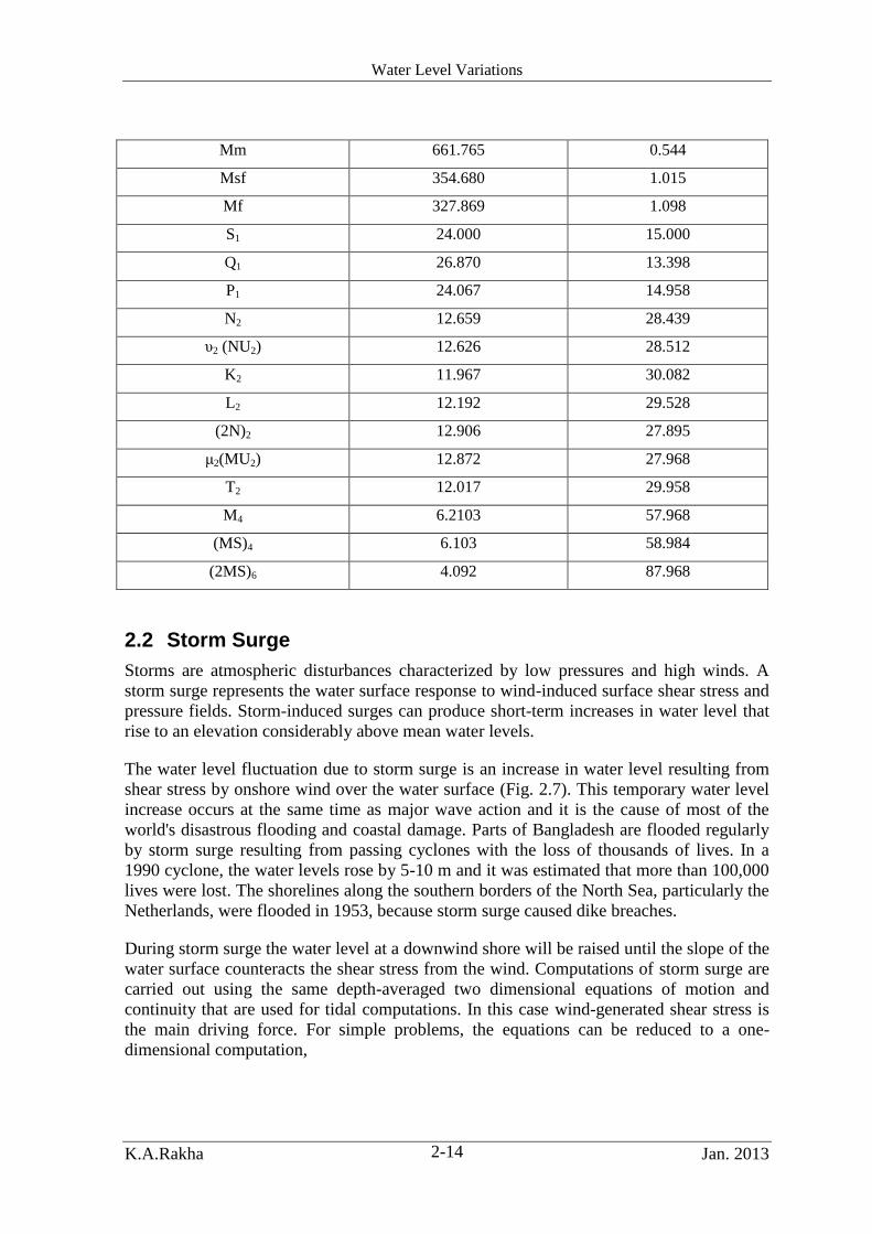
Water Level Variations
K.A.Rakha Jan. 2013 2-14
Mm 661.765 0.544
Msf 354.680 1.015
Mf 327.869 1.098
S1 24.000 15.000
Q1 26.870 13.398
P1 24.067 14.958
N2 12.659 28.439
υ2 (NU2) 12.626 28.512
K2 11.967 30.082
L2 12.192 29.528
(2N)2 12.906 27.895
μ2(MU2) 12.872 27.968
T2 12.017 29.958
M4 6.2103 57.968
(MS)4 6.103 58.984
(2MS)6 4.092 87.968
2.2 Storm Surge
Storms are atmospheric disturbances characterized by low pressures and high winds. A
storm surge represents the water surface response to wind-induced surface shear stress and
pressure fields. Storm-induced surges can produce short-term increases in water level that
rise to an elevation considerably above mean water levels.
The water level fluctuation due to storm surge is an increase in water level resulting from
shear stress by onshore wind over the water surface (Fig. 2.7). This temporary water level
increase occurs at the same time as major wave action and it is the cause of most of the
world's disastrous flooding and coastal damage. Parts of Bangladesh are flooded regularly
by storm surge resulting from passing cyclones with the loss of thousands of lives. In a
1990 cyclone, the water levels rose by 5-10 m and it was estimated that more than 100,000
lives were lost. The shorelines along the southern borders of the North Sea, particularly the
Netherlands, were flooded in 1953, because storm surge caused dike breaches.
During storm surge the water level at a downwind shore will be raised until the slope of the
water surface counteracts the shear stress from the wind. Computations of storm surge are
carried out using the same depth-averaged two dimensional equations of motion and
continuity that are used for tidal computations. In this case wind-generated shear stress is
the main driving force. For simple problems, the equations can be reduced to a one-
dimensional computation,

Water Level Variations
K.A.Rakha Jan. 2013 2-15
gD
U
dx
dS2
cos
( 2.2 )
where S is the storm surge (the setup of the water level by the wind), x is the direction over
which the storm surge is calculated, ζ is a constant (=3.2x10⁻⁶
), U is the wind speed, φ is
the angle between the wind direction and the x-axis and D is the new depth of water
(=d+S). Equation 2.2 clearly shows that storm surge is greatest in shallow water.
2.3 Barometric Surge
Since strong winds are the result of large pressure fluctuations, a barometric surge will
accompany storm surge. Suppose there is a difference in barometric pressure Δp between
the sea and the shore, then an additional water level Δh rise will be generated:
g
ph
( 2.3 )
where ρ is the density of water. Equation 2.3 results in a water level rise of about 0.1 m for
each kPa of pressure difference. A major depression can easily generate a pressure
difference of 5 kPa, resulting in a potential barometric surge of 0.5 m.

Water Level Variations
K.A.Rakha Jan. 2013 2-16
Fig. 2.7: Storm surge in closed and open seas.
s
W
d
D sW
Closed Basin
Open Sea
s
W
s
W
d
D sW
d
D sW
Closed Basin
Open Sea

Water Level Variations
K.A.Rakha Jan. 2013 2-17
2.4 Seiche
Seiches are standing waves or oscillations of the free surface of a body of water in a closed
or semiclosed basin. These oscillations are of relatively long period, extending from
minutes in harbors and bays to over 10 hr in the Great Lakes. Any external perturbation to
the lake or embayment can force an oscillation. In harbors, the forcing can be the result of
short waves and wave groups at the harbor entrance.
The oscillations will continue for some time because friction forces are quite small. The
wave length of the fundamental mode of the oscillation (a standing wave) for a closed
basin (Fig. 2.8) is twice the effective basin length (B). In general, the wave length is
2B/(1+nh) for the nh harmonic. For an open ended basin (open coast), the fundamental
wave length is 4 times the effective length of the shelf (B) over which the storm surge was
initially set up. In general, for the nh harmonic it is 4B/(1+2nh). The period of oscillation
(T=L/C) for a closed basin may be calculated as:
Fig. 2.8: Seiche wavelengths.
L/2
B
2L1/2
3L1/4
B
L/4
Open Basin Closed Basin
L/2
B
2L1/2
3L1/4
B
L/4
Open Basin Closed Basin

Water Level Variations
K.A.Rakha Jan. 2013 2-18
2.5 Tsunami
Tsunami is a single wave generated by sub-sea earthquakes and typically has a period of 5
to 60 minutes. Tsunami waves can travel long distances and is normally not very high in
deep water. In shallow water the wave shoaling can reach a height more than 10 m.
Tsunamis are rare and coastal structures seldom take them into account.
2.6 Eustatic (Sea) Level Change
The term Eustatic refers to a global change in ocean water levels; the result of melting or
freezing of the polar ice caps and the thermal expansion of the water mass with
temperature change. The water levels 25,000 years ago were 150 m below the present level
(Kamphuis, 2000). Between then and 3,000 years ago, water level rose at a more-or-less
steady rate of about 7 mm/yr to almost the present water level. The present average rate of
eustatic rise is small and therefore difficult to measure. Estimate range from 1 to 3 mm/yr.
This relatively small rate of rise, nevertheless, causes the ocean shores to be submerging
and is at least partly responsible for the fact that most beaches around the world are
eroding over the long term.
2.7 Isostatic (Land) Rebound and Subsidence
The common natural cause for isostatic (land) elevation change is a result of the
adjustment of the earth's crust to the release of pressure exerted by the 1 to 2 km thick ice
sheet that covered it during the last glaciation. Typically, the earth’s crust was severely
depressed by the ice and a rise (forebulge) was formed in the earth’s crust ahead of the
glaciers. When the ice retreated, the earth's surface rebounded (upward) where the glaciers
had been and lowered where the forebulge had occurred. This process still takes place
today, but at a much reduced rate. Most areas in the higher latitudes experience isostatic
rebound and areas at more intermediate latitudes experience some subsidence.
Although subsidence does occur naturally, often it is man-made. Pumping groundwater,
petroleum and natural gas are common causes. Subsidence exacerbates the effects of
eustatic sea level rise since the relative sea level rise with respect to the land will now be
greater.

Water Level Variations
K.A.Rakha Jan. 2013 2-19
Fig. 2.9: Tsunami generation and propagation.

Water Level Variations
K.A.Rakha Jan. 2013 2-20
2.8 Global Climate Change
The final and potentially most dangerous water level change results from trends in global
climate. In the discussion of eustatic sealevel rise, we have already seen that global
warming after the last glaciation has resulted in a sealevel rise of 100 to 150 m through
melting of the polar ice caps and thermal expansion of the water in the ocean. The present
rate has slowed down to 1 to 1.5 mm/yr, but any additional warming would increase this
rate of sealevel rise.
Concern is centered around the production of the so-called greenhouse gases. These
combustion products are thought to act as an insulating blanket over the earth, decreasing
the net longwave radiation from the earth into space and thus trapping the sun's heat to
cause global warming. It is a controversial subject and indeed there is a contingent of
respected scientists that disputes the whole idea.
According to Kamphuis (2000), predicted rise in water level for the year 2025 varies from
0.1 to 0.2 m. For 2050, the estimates vary from 0.2 to 1.3 m and for 2100 the estimates are
0.5 to 2 m.

3 Currents in the Marine Environment
Various types of currents exist in the marine environment. These currents may exist in the
open sea or in the nearshore area. In the open sea the currents are mainly tidal and wind
driven currents. In the nearshore area wave induced currents can also exist.
3.1 Tidal Currents
Tidal currents are induced by the gravity forces of the sun, the moon, and the planets. Tidal
currents are oscillatory currents with typical periods of about 12 or 24 hours (semi-diurnal
and diurnal). Tidal currents are influenced by the sea bottom contours and by coastal
morphology. They are strongest at large water depths and in estuaries or straits where the
current is forced into a narrow area. The most important tidal currents for coastal
morphology are the currents generated at tidal inlets.
In the deep, open ocean, the fluid velocity (tidal current or horizontal tide) is in phase with
the tidal water level fluctuations (vertical tide). At high water there is a maximum current
velocity in the direction of tide propagation. When the tide approaches land, however, the
phase relationship between horizontal and vertical tide changes. In the case of a tidal inlet
or bay, the water level fluctuations in the bay are driven by the tidal water level in the sea.
Rising water levels in the sea cause a current to flow into the bay, raising its water level.
This inflow of water is called flood and the outflow current during the other half of the
tidal cycle is called ebb.
3.2 Wind Generated Currents
Wind generated currents are caused by the wind shear stress along the sea surface. These
currents are normally located in the upper layer of the water body and are thus not very
important from a morphological point of view. Wind currents can have an important role
however in the movement of pollutants and oil spills. In shallow waters and in lagoons,
wind generated currents can be important. Wind generated currents are typically less than 5
per cent of the wind speed.
3.3 Stratification and Density Currents
An estuary is defined as a tidal area where a river meets the sea. It has salt water on its
downstream limit (sea) and fresh water on the upstream limit (river). The salt sea water
normally has a salinity in the vicinity of 35 parts per thousand (ppt) and a density of 1035
kg/m3. The fresh water has a density of 1000 kg/m3.
The way the transition from salt to fresh water takes place depends on the amount of
mixing that takes place in the estuary. In a well-mixed estuary (an estuary with much
turbulence), salt and fresh water are thoroughly mixed at any location. Salinity simply
varies along the estuary from 35 ppt in the sea to zero ppt in the river and at any specific
location, salinity and density will vary with the tide.
If there is little mixing in the estuary, the lighter fresh water will lie over the heavier salt
water, resulting in a stratified estuary. The density differences will induce currents. In deep

Currents in the Marine Environment
K.A.Rakha Jan. 2013 3-2
oceans, density currents also exist due to stratification caused by temperature and salinity
differences over the water depth.
3.4 Wave Induced Currents
Besides the wave-induced oscillatory currents the breaking of waves induces other non-
oscillatory currents. These currents are directed in the on/offshore and alongshore
directions.
3.4.1 Shore-normal currents
The breaking phenomena and the asymmetric wave form in the nearshore area results in a
mass transport of water with in the upper layers. This results in a water surplus in the surf
zone (wave setup). This surplus water returns to the sea via rip and undertow currents.
3.4.1.1 Rip Currents
At certain intervals along the coastline, the longshore current will form a rip current. The
rip currents are directed in the offshore direction. The rip opening in the bars will often
form the lowest section of the coastal profile with a local setback in the shoreline opposite
the rip opening (see Fig. 3.1). Field observations showed that the rip current velocity might
exceed 1.0 m/sec and occasionally extend more than 500 m from the breaker line.
Presently there is no proven method to predict rip current generation and the spacing
between rips.
Figure 3.2 shows the typical nearshore currents for different wave incidence (Harris, 1969).
3.4.1.2 Undertow
The undertow current is a return flow concentrated near the bed (see Fig. 3.3). This current
is important in the formation of bars. The mass transport carried toward the beach due to
waves is concentrated between the wave trough and crest elevations. Because there is no
net mass flux through the beach, the wave-induced mass transport above the trough is
largely balanced by a reverse flow or undertow below the trough. The undertow current at
the bottom may be relatively strong, generally 8-10 percent of the wave celerity.
The wave setup at the still water line is about 0.15db.
3.4.2 Shore-parallel currents
Longshore currents are the dominating current in the nearshore zone, generated by
obliquely approaching breaking waves. This current has its maximum close to the breaker
line (see Fig. 3.2). During storms the longshore current can reach values of 2.5 m/s. The
longshore current carries sediment along the shoreline (littoral drift) as explained later.

Currents in the Marine Environment
K.A.Rakha Jan. 2013 3-3
Fig. 3.1: Photo of rip currents observed along a beach.

Currents in the Marine Environment
K.A.Rakha Jan. 2013 3-4
Fig. 3.2: Nearshore Circulation systems (Harris, 1969)
Vl
b
Rip
Current
Breaker
Typical
current
distribution
A. Oblique (b large)
B. Normal (b ~ 0)
C. Slightly Oblique (b small)
b
Vl
b
Rip
Current
Breaker
Typical
current
distribution
A. Oblique (b large)
B. Normal (b ~ 0)
C. Slightly Oblique (b small)
b

Currents in the Marine Environment
K.A.Rakha Jan. 2013 3-5
Fig. 3.3: Schematic of the undertow current.
Undertow
MWL
SWL
Wave Setup
Undertow
MWL
SWL
Wave Setup

Currents in the Marine Environment
K.A.Rakha Jan. 2013 3-6
3.4.3 Two-dimensional Currents
Along a straight coastline the above mentioned shore parallel and shore normal currents
exist. When, combined they are three-dimensional in nature. For complex bathymetries
two dimensional currents exist. These currents occur due to irregular bathymetries or due
to the existence of structures in the nearshore zone (such as groins or breakwaters).
Coastal structures influence the current pattern in two ways: by obstructing the shore-
parallel currents and by setting up secondary circulation currents. The nature of the
obstruction to the shore-parallel currents depends on the extent and geometry of the coastal
structure. If the structure is located within the breaker zone, the obstruction leads to
offshore directed currents that will cause loss of beach material. If the structure is a
harbour, the current will follow the upstream breakwater and reach the entrance area (see
Fig. 3.4). These currents will cause sedimentation and will affect the navigation. It is thus
important to provide smooth currents that will be acceptable for the navigation and will
reduce the sedimentation. A smooth layout of the main and secondary breakwaters with a
narrow entrance is the best alignment, rather than the alignment provided in Fig. 3.4.
At the leeward side of coastal structures, special current patterns can develop caused by the
sheltering effect of the structure in the diffraction area. The wave setup in the sheltered
areas will be lower than that in the adjacent exposed areas generated a gradient in water
level that will drive currents (e.g. see Fig. 3.5). These circulation currents can be dangerous
to swimmers who might swim in the sheltered areas during storms.
If the structure extends beyond the breaker zone, the shoe parallel current will be directed
along the structure where the increasing depth will cause the currents to be reduced. This
will cause the deposition of sediment forming a shoal off the breaker zone. In the lee of a
major coastal structure the effect of return currents towards the sheltered area will also be
pronounced. In this case however, the current patterns will be smoother and less dangerous
for swimmers.

Currents in the Marine Environment
K.A.Rakha Jan. 2013 3-7
Fig. 3.4: Schematic of the currents at the SUMED Harbour at Sedi Kerir, Egypt
(Rakha and Abul-Azm, 2003)

Currents in the Marine Environment
K.A.Rakha Jan. 2013 3-8
Fig. 3.5: Measured flow field behind a breakwater (Mory and Hamm, 1995)
3.5 Hydrodynamic Models
The physical understanding and the mathematical modeling of hydrodynamic processes in
the nearshore zone is important for coastal engineers and for those involved in coastal zone
management. Hydrodynamic (HD) computations represent the core of any simulation for
water quality, siltation, and morphology studies. The development of a robust and flexible
HD model could be regarded as the first step towards the development of a fully integrated
modeling system capable of modeling hydrodynamics, sediment transport, morphological
processes and water quality.
HD models vary from fully three dimensional 3D to simpler one dimensional 1D models.
For such models they may differ in the choice of the numerical grid, the discretization

Currents in the Marine Environment
K.A.Rakha Jan. 2013 3-9
method, the time difference scheme, the solution technique, and the treatment of boundary
conditions.
Many HD models have been developed for the prediction of tidal and wind induced
currents. These models have been applied to oceans and seas or smaller areas such as tidal
inlets and harbour. These models are usually based on the hydrostatic pressure assumption
resulting in the shallow water equations.
Wave-driven currents describe the mean motion that is generated in coastal areas where
wind-generated short waves refract, shoal, diffract or break. The spatial variation of wave
momentum, the gradients of the radiation stresses, is the main driving force. The wave-
induced current diminishes rapidly away from the coast. This current is important in
limited areas where the water depth is much smaller than the wave-length and intensive
wave deformation is taking place. Generation of currents by waves includes longshore,
undertow, and rip currents.
Models for wave-driven currents vary from simple models that predict the longshore
currents over the beach profile to more detailed 2D models that predict the depth averaged
currents. Other models have been developed that calculate the undertow distribution over
the water depth. More detailed models have been developed that impose the vertical profile
of the longshore current and the undertow on the 2D depth integrated currents resulting in
the so called Quasi-3D models.

4 Nearshore Sediment Transport
The breaking waves and the nearshore currents transport beach sediments. Sometimes this
transport results only in a local rearrangement of sand into bars and troughs, or into a series
of rhythmic embayments cut into the beach. At other times there are extensive longshore
displacements of sediments, possibly moving hundreds of thousands of cubic meters of
sand along the coast each year.
A distinction is made between two modes of sediment transport: suspended sediment
transport, in which sediment is carried above the bottom by the turbulent eddies of the
water, and bed-load sediment transport, in which the grains remain close to the bed and
move by rolling and saltating. Although this distinction may be made conceptually, it is
difficult to separately measure these two modes of transport on prototype beaches.
The longshore sediment transport rate is directed parallel to the coast and is among the
most important nearshore processes that control the beach morphology, and determines in
large part whether shores erode, accrete, or remain stable. An understanding of longshore
sediment transport is essential to sound coastal engineering design practice.
Sediment is also transported in the on/offshore direction causing changes in the beach
profile. The seasonal changes in the beach profile are caused by the on/offshore transport
of sediment. Figure 4.1 provides a sketch for different definitions along a beach profile.
Sediment transport can also result from the currents generated by alongshore gradients in
breaking wave height due to the sheltering effect. This transport is manifest as a movement
of beach sediments toward the sheltered area. The result is transport in the “upwave”
direction on the downdrift side of the structure. This, in turn, can create a buildup of
sediment on the immediate, downdrift side of the structure.
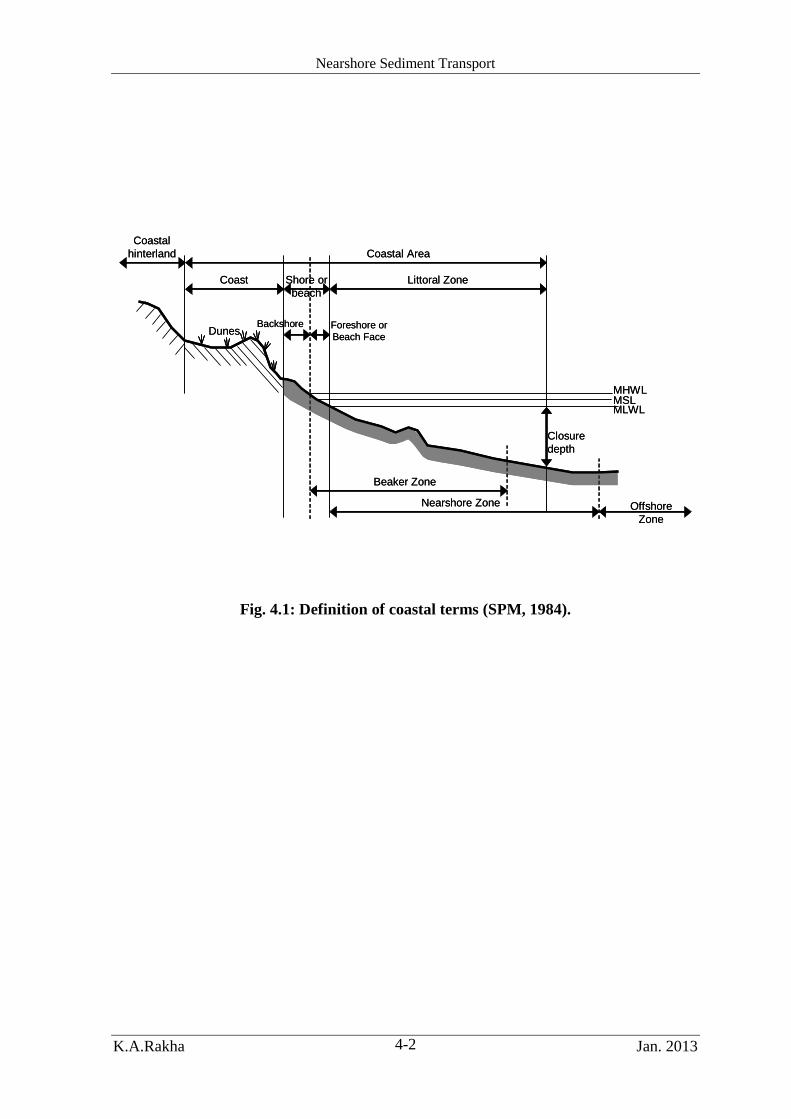
Nearshore Sediment Transport
K.A.Rakha Jan. 2013 4-2
Fig. 4.1: Definition of coastal terms (SPM, 1984).
MHWL
MLWLMSL
Dunes
Coastal
hinterland Coastal Area
Littoral ZoneShore or
beach
Coast
Backshore Foreshore or
Beach Face
Beaker Zone
Closure
depth
Nearshore Zone Offshore
Zone
MHWL
MLWLMSL
Dunes
Coastal
hinterland Coastal Area
Littoral ZoneShore or
beach
Coast
Backshore Foreshore or
Beach Face
Beaker Zone
Closure
depth
Nearshore Zone Offshore
Zone

Nearshore Sediment Transport
K.A.Rakha Jan. 2013 4-3
4.1 Longshore Sediment Transport
The movement of beach sediment along the coast is referred to as littoral transport or
longshore sediment transport, whereas the actual volumes of sand involved in the transport
are termed the littoral drift. This longshore movement of beach sediments is of particular
importance in that the transport can either be interrupted by the construction of jetties and
breakwaters (structures which block all or a portion of the longshore sediment transport),
or can be captured by inlets and submarine canyons. In the case of a jetty, the result is a
buildup of the beach along the updrift side of the structure and an erosion of the beach
downdrift of the structure. The impacts pose problems to the adjacent beach communities,
as well as threaten the usefulness of the adjacent navigable waterways.
4.1.1 Predicting Potential Littoral Drift
Littoral transport is often described under the assumption that the shoreline is nearly
straight with nearly parallel depth contours. This assumption is very often valid for
relatively short sections of the shore and for smooth transitions assumed between such
sections. If unlimited amounts of sand are assumed to exist over the active beach profile,
the potential sediment transport rates can be estimated. The longshore sediment transport
rates can be estimated using bulk or detailed formulations.
4.1.1.1 Bulk Formulations
In these types of formulations the longshore sediment transport rate Qs is calculated from a
semi-empirical formula. The well know CERC formula (SPM, 1984) is an example of such
a formula and can be written as,
bsb
s
HQ
2sin10*2.2
2/56
(4.1)
Where Hsb is the significant wave height at the breaker, b is the breaker wave angle (see
Figs. 3.2 and 4.2), is the breaker index (Hb/db) and the subscript b denotes the breaker
line. It can be seen that this formula does not include some parameters that will definitely
have an effect on the littoral drift such as the grain size. The Kamphuis (1991) formula
includes more parameters and can provide better estimates for the littoral drift. This
formula can be written as,
bbopsbs DmTHQ 2sin10*4.6 6.025.075.05.124 (4.2)
where m is the beach slope, D is the grain size, and the subscript p denotes the peak wave
period.
Figure 4.2 shows the effect of the wave height and the angle of incidence on the littoral
drift as predicted from the Kamphuis (1991) formula.
The GENESIS model (part of the CEDAS package) uses such a bulk formulation for
calculating the sediment drift.

Nearshore Sediment Transport
K.A.Rakha Jan. 2013 4-4
4.1.1.2 Detailed Formulations
In these formulations, the sediment transport rates are calculated over the beach profile and
integrated over the profile to determine the littoral drift. Many different models exist for
the calculations at a single location ranging from simpler models based on equations for
calculating the sediment transport rates (e.g. UNIBEST) to models that calculate the
suspended sediment concentration over the full water depth (e.g. LITPACK model).
4.1.2 Littoral Drift Budget
A littoral drift budget is the sum of littoral transport contribution by all the possible
combinations of wave heights and directions (determined from the nearshore wave rose).
At a particular beach site the transport might be to the right (to East as in Fig. 4.2) during
part of the year and to the left during the remainder of the year. If the left and right
transports are denoted respectively QsL and QsR, with QsR being assigned a positive
quantity and QsL assigned a negative value for transport direction clarification purposes,
then the net annual transport is defined as Qs NET = QsR + QsL. The net longshore sediment
transport rate is therefore directed right and positive if QsR > QsL, and to the left and
negative if QsR < |QsL|. The net annual transport can range from essentially zero to a large
magnitude, estimated at a million cubic meters of sand per year for some coastal sites.
The gross annual longshore transport is defined as Qs GROSS = QsR + |QsL|, the sum of the
temporal magnitudes of littoral transport irrespective of direction. It is possible to have a
very large gross longshore transport at a beach site while the net transport is effectively
zero.
These two contrasting assessments of longshore sediment movements have different
engineering applications. For example, the gross longshore transport may be utilized in
predicting backfilling rates in navigation channels and uncontrolled inlets, whereas the net
longshore transport more often relates to the deposition versus erosion rates of beaches on
opposite sides of jetties or breakwaters.
An important parameter in relation to the littoral drift conditions is the variation of the net
transport with any variation in the coastline orientation. If for example a groin is
constructed along a beach, it will initially block the sediment resulting in a zero net
transport rate at the groin. Thus sand will accrete upstream of the groin forming a coastline
with an orientation that produces a zero net transport rate. The efficiency of the groin
depends very much on the angle between the present coastline and the zero net littoral drift
coastline orientation. If this angle is small, the groin will be efficient as it will be able to
create a long accreting area. If the angle is large, the groin will influence a very short part
of the coastline and thus groins will not be useful for such areas.

Nearshore Sediment Transport
K.A.Rakha Jan. 2013 4-5
Fig. 4.2: Effect of different parameters on the littoral drift.
b
Normal to
Coastline
Coastline
-ve +veWave fro
nt
-90 -60 -30 0 30 60 90
Qs
0 1 2 3 4
Hs (m)
Qs
To
East
To
West
b
Normal to
Coastline
Coastline
-ve +veWave fro
ntb
Normal to
Coastline
Coastline
-ve +veWave fro
nt
-90 -60 -30 0 30 60 90
Qs
0 1 2 3 4
Hs (m)
Qs
To
East
To
West

Nearshore Sediment Transport
K.A.Rakha Jan. 2013 4-6
4.2 On/Offshore Sediment Transport
Varying the wave conditions, results in varying onshore and offshore transport rates over
the beach profile. These transports are to some extent reversible and therefore irrelevant in
terms of longshore sediment transport.
When the beach profile is exposed to high wave conditions, sediment near the shoreline
will be transported offshore and typically be deposited in a bar resulting in an overall
flattening of the shoreface (winter profile). The foreshore however will get steeper and the
shoreline will recede. During following periods of lower wave conditions and swell, the
bar will slowly move towards the shoreline and the profile will be rebuilt (summer profile).
Figure 4.3 provides a schematic of the summer and the winter beach profiles.
It is important to take into account these temporary profile changes to avoid erosion of the
coast. Thus, a sufficient setback is essential when designing any structures in the coastal
area.
The on/offshore sediment transport is closely related to the form of the coastal profile.
Several investigations showed that a coastal profile possesses an average, characteristic
form referred to as a theoretical equilibrium profile. A well known equation for
representing the equilibrium profile was proposed by Dean (1977),
3
2
Axd (4.3)
where A is a constant that depends on the mean grain size, and x is the offshore direction.
The equilibrium profile is valid till the closure depth that can be calculated from
(Hallemeyer, 1978),
2
2
12,
12, 5.6828.2s
s
scgT
HHd
(4.4)
where Hs,12 is the significant wave height exceeded 12 hour per year, and Ts is the
corresponding significant wave period.

Nearshore Sediment Transport
K.A.Rakha Jan. 2013 4-7
Fig. 4.3: Schematic of summer and winter beach profiles.
4.3 Coastal Sediment Cells
The coastline is a series of interlinked physical systems, comprising both offshore and
onshore elements. Sediment (clay, silt, sand, gravel etc.) is moved around the coast by
waves and currents in a series of linked systems (sediment transport cells). Simple cells
comprise an arrangement of:
Sediment source areas (e.g. eroding cliffs, rivers, the sea bed);
Areas where sediment is moved by coastal processes; and
Sediment sinks (e.g. beaches, estuaries or offshore sinks).
Along a particular stretch of coast there may be a series of such cells, often operating at
different scales. In contrast to river catchments, coastal systems have no obvious
boundaries. Suspended sediments, for example, may be carried thousands of miles around
the coast. Although headlands can be identified which appear to mark the limits of coarse
sediment transport, they are often not permanent boundaries.
Winter Bar Profile
Summer Berm Profile
Winter Bar Profile
Summer Berm Profile
Nearshore Sediment Transport
K.A.Rakha Jan. 2013 4-8
4.4 Sediment Transport Models
As discussed earlier sediment is brought in suspension by the waves and the currents and
transported by the currents. For fine sediment the advection dispersion model described
above is used to predict the movement of sediment by tidal currents. The settling of
sediment and the erosion of sediment from the bed must be included in such models.
For sediment transported by the wave-induced currents, different types of models exist.
These models range from simple formulas used to calculate the longshore sediment
transport rates (as discussed earlier) to more detailed models. The detailed models calculate
the vertical variation in turbulent energy, currents, and suspended sediment. The STP
model of DHI Water and Environment is an example of such a model (see Fig. 4.4).
The LITPACK model includes many different models that obtain data from the STP
model. These models are tailored for different applications. The LITDRIFT model is used
to calculate the littoral drift. LITLINE is a shoreline model use to calculate the shoreline
changes as explained later. LITTREN is used to calculate the filling of a trench and finally
LITPROF calculated the beach profile changes due to on/offshore sediment transport.
Other wave-induced sediment transport models, calculate the sediment transport rates from
formulas based on the depth averaged currents (from a 2D HD model) and the wave
conditions (from a wave model).

Nearshore Sediment Transport
K.A.Rakha Jan. 2013 4-9
Fig. 4.4: Different models in the LITPACK package of DHI.
STP
LITDRIFT
LITLINE
LITTREN
LITPROF
STP
LITDRIFT
LITLINE
LITTREN
LITPROF
Nearshore Sediment Transport
K.A.Rakha Jan. 2013 4-10
4.4.1 Morphology and Shoreline Change Models
Morphology models calculate the changes in the bathymetry due to the waves and currents.
De Vriend et al. (1993) classified the different types of morphology models into four
categories; coastline models, coastal profile models, coastal area models, and local models.
A flow chart of a typical process type coastal area model is shown in Fig. 4.5. In such
models several modules are required. A wave module, a hydrodynamic module, a sediment
transport module, and a sediment balance module. The accuracy of the morphology model
will thus depend on the accuracy of each module. Thus, it is essential to choose modules
that are compatible.
Such process type morphology models will require extensive computer time and can not be
applied to simulate long term changes in the morphology. Thus, shoreline models (as
explained later) are commonly used for such purposes. The LITLINE model of Fig. 4.4 is
an example of such models. These models simulate the movement of the shoreline
assuming no changes in the beach profile.
4.5 One-line Models
One-line models used to estimate longshore sand transport rates and long-term shoreline
changes generally assume that the profile is displaced parallel to itself in the cross-shore
direction. The profile may include bars and other features but is assumed to always
maintain the same shape. This assumption is best satisfied if the profile is in equilibrium.
The one-line model is formulated on the conservation equation of sediment in a control
volume or shoreline reach, and a bulk longshore sand transport equation. It is assumed that
there is an offshore closure depth dC (Fig. 4.6) at which there are no significant changes in
the profile, and the upper end of the active profile is at the berm crest elevation dB. The
constant profile shape moves in the cross-shore direction between these two limits. This
implies that sediment transport is uniformly distributed over the active portion of the
profile. The incremental volume of sediment in a reach is simply (dB + dC)∆x∆y, where ∆x
is the reach of shoreline segment, and ∆y is the cross-shore displacement of the profile.
Conservation of sediment volume may be written,
0)(
1
q
x
Q
ddt
y s
cB
(4.5)
where, y is the shoreline position, t is time, dB is the berm height, dc is the closure depth, q
is a source or sink in sediment and Qs is the longshore sand transport rate (m3/sec). The co-
ordinate system x and y-directions are defined in Fig. 4.6. The value of Qs is calculated
from formulas similar to those described earlier.

Nearshore Sediment Transport
K.A.Rakha Jan. 2013 4-11
Fig. 4.5: Flow chart of typical process type morphology model.
Sediment
Balance
Wave
Field
Bed
Topography
Sediment
Transport
Current
Field Time
Stepping
Sediment
Balance
Wave
Field
Bed
Topography
Sediment
Transport
Current
Field Time
Stepping

Nearshore Sediment Transport
K.A.Rakha Jan. 2013 4-12
Fig. 4.6: Schematic for terms used in One-line models.
4.5.1 Analytical Solution
If the angle of the shoreline is small with respect to the x axis and simple relationships
describe the waves, analytical solutions for shoreline change may be developed. As an
example, assuming that the breaking wave angle αb is small, the following planform
shoreline change equation can be derived,
02
2
x
yD
t
y (4.6)
Where
d
qD
2 (4.7)
where d = dc + dB and q is determined from,
dx
dyqqQ be 2sin2sin (4.8)
where is defined as the angle between the wave crest and the x-axis.
y
dB
Q t
dC
Y x
X
tXX

Nearshore Sediment Transport
K.A.Rakha Jan. 2013 4-13
A number of researchers have employed this equation or slight variations of it to provide
analytical solutions to shoreline change under certain assumptions (the boundary
conditions and initial conditions of the problem).
Pelnard-Considére (1956) first presented an analytical solution to this simplified shoreline
change equation for the case of an impermeable groin or jetty impounding the longshore
sand transport on the updrift side of the structure under a stationary (constant) wave
climate (Fig. 4.7).
The following equation was derived,
)(tan4 2
uerfcueDt
y u
b
(4.9)
where, t is the time and
Dt
xu
4 (4.10)
the erfc can be approximated from the following equation,
2
54321)( ueTAATATATATuerfc (4.11)
where
A1= 0.254829592
A2= -0.284496736
A3= 1.421413741
A4= -1.453152027
A5= 1.061405429
and
PuT
1
1 (4.12)
where P = 0.3275911.
The time required for the structure to fill to capacity t = tf can be found by setting x = 0 and
y to the barrier length S,
b
fD
St
2
2
tan4 (4.13)

Nearshore Sediment Transport
K.A.Rakha Jan. 2013 4-14
Fig. 4.7: Schematic for case of complete barrier.
Yo
S
bbdx
dy tan
Shoreline at time t
Original Shoreline X
Y

Nearshore Sediment Transport
K.A.Rakha Jan. 2013 4-15
4.5.2 Model Classification according to Time and Space
According to Kamphuis (2000), models can be classified according to the time and space
(area) covered. Figure 4.8 identifies Short Term Small Area Models (S), Medium Term
Medium Area Models (M) and Long Term Large Area Models (L). The exact definitions
of S, M and L will obviously be a function of the problem to be solved. Some typical
definitions are: S-models cover prototype durations of hours (or less) and areas of 1 to 100
m2. Coastal applications are models of bedforms (ripples and dunes), breakwater cross-
sections, local scour near structures, water intakes, sewerage outfalls and diffusers.
M-models typically cover prototype areas of several km2 and durations of years. Coastal
applications are models of shore sections (littoral cells), harbors, inlets, estuaries or
portions of estuaries, and shore protection with offshore structures. This category also
includes fluid flow models (waves and currents) that cover medium areas, although they
may only represent a short duration. Examples are refraction and diffraction of a single
wave condition. We include them under M models because their outcome is normally
applied to medium term problems such as wave agitation in a harbor and coastal
morphology.
L-models typically cover areas greater than 100 km2 over centuries. Examples are models
representing the shoreline evolution of sections covering thousands of years, or the
development of all or a portion of river deltas over centuries.
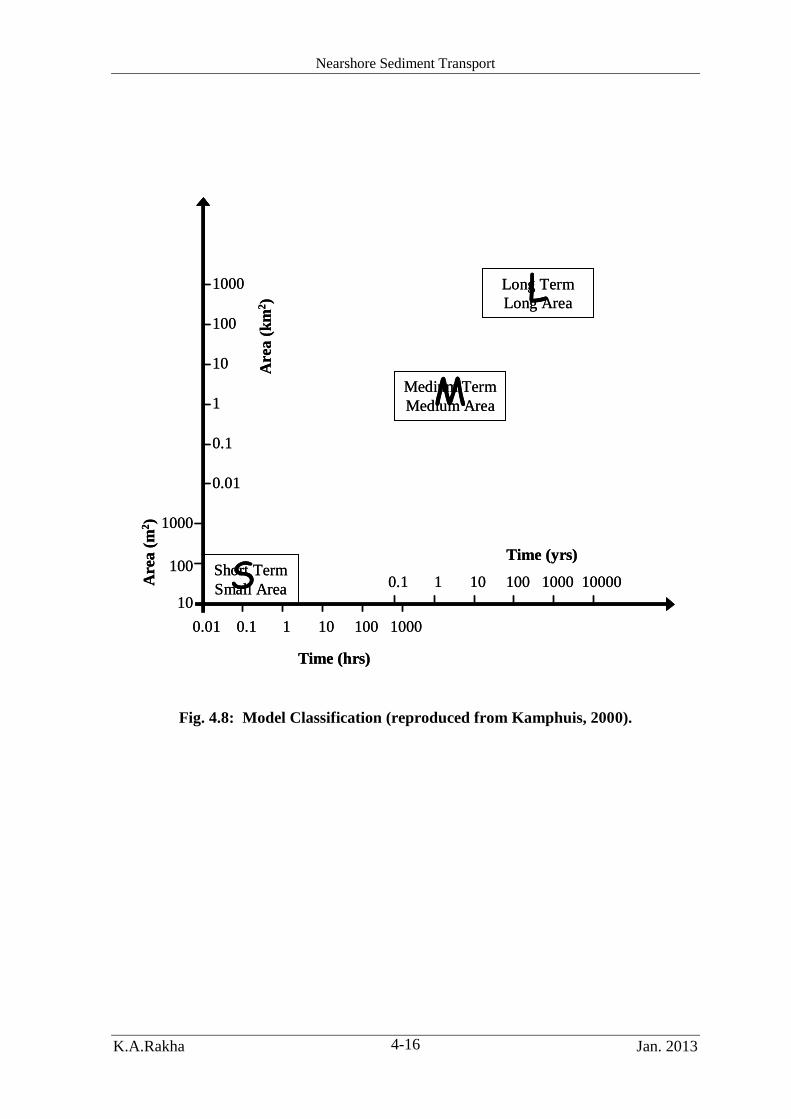
Nearshore Sediment Transport
K.A.Rakha Jan. 2013 4-16
0.01 0.1 1 10 100 1000
0.1 1 10 100 1000 10000
Time (yrs)
Time (hrs)
100
1000
0.01
10
0.1
1
10
100
1000
Are
a (
km
2)
Are
a (
m2)
Short Term
Small Area
Medium Term
Medium Area
Long Term
Long Area
S
M
L
0.01 0.1 1 10 100 1000
0.1 1 10 100 1000 10000
Time (yrs)
Time (hrs)
100
1000
0.01
10
0.1
1
10
100
1000
Are
a (
km
2)
Are
a (
m2)
Short Term
Small Area
Medium Term
Medium Area
Long Term
Long Area
S
M
L
Fig. 4.8: Model Classification (reproduced from Kamphuis, 2000).

Nearshore Sediment Transport
K.A.Rakha Jan. 2013 4-17
Contrary to physical models, in numerical modeling, a problem must be clearly understood
before a model can be properly formulated so that it produces valid solutions. Equations
governing the processes, numerical methods, transfer functions and calibration coefficients
must all be known, at least approximately, from the outset. In many cases many constants
and coefficients used in numerical models are not so well known. For example, we only
know dispersion coefficients within one or two orders of magnitude, most of the time.
Thus, because of uncertainties in the equations and the coefficients, and because of
approximations made in the numerical simulation of the equations, numerical modeling
results can only produce qualitative results, at best. Interpretation of such qualitative results
into quantitative estimates is the major task of numerical modeling. It requires a thorough
understanding of the coastal processes, the applicable equations, the various interactions
between variables and the shortcomings in evaluation of the coefficients. In addition, just
as the physical modeler needs to know about scaling, scale effects and laboratory effects,
the numerical modeler needs to understand the implications of simplifications brought into
the model, and numerical modeling methods with its pitfalls, such as instabilities,
numerical diffusion and dispersion, smoothing, etc.
For some problems we know enough about the equations and coefficients to model them
numerically with some confidence. Such tractable problems as fluid flow with relatively
simple boundary conditions can be modelled using either physical models or numerical
models, combining long waves, short waves and currents. Once numerical models can be
successfully applied to solve a type of problem, the use of physical models for such a
problem will decline.
4.5.3 Reducing Uncertainty
Physical and numerical models produce results with some degree of uncertainty. The
uncertainties vary from model to model depending on the capability of the model to
accurately represent the physical processes at hand. Wave models for example have less
uncertainty than sediment transport models.
The uncertainties in model results can be reduced through proper model validation, which
consists of
Benchmarking,
Calibration,
Verification.
Any numerical model, regardless of its sophistication, should be properly benchmarked.
The model must be run for simple boundary conditions and with simplified equations to be
compared with analytical solutions. For example, a 1D shoreline model must be able to
simulate diffusion-type solutions of Pelnard Considère (1956), before it can be successfully
applied to more complex situations.
In calibration, the model parameters are adjusted so that the model reproduces measured
prototype values. The concept of model calibration is based on the fact that directly
measured prototype parameters contain less uncertainty than the output of the model,
Nearshore Sediment Transport
K.A.Rakha Jan. 2013 4-18
which is based on the combined uncertainties of the input data and the model. Thus it
makes good sense to calibrate the model sediment transport rate using prototype
bathymetry measurements. For example a hydrodynamic model that calculates the tidal
currents in a coastal lagoon can be calibrated by comparing the predicted currents with
actual field measurements.
Calibration can consist of several intermediate stages. A coastal morphology model can
first be calibrated for wave heights, current directions and magnitudes, velocity
distributions, and sediment transport rates and their distributions, before being calibrated
for final changes in morphology. If the model is only calibrated for the currents, then the
uncertainty in the morphology calculations will still remain. This is often the case for
advection dispersion modeling, where the hydrodynamic model is calibrated against
measurements of the currents whereas the advection dispersion model is not calibrated.
This results in uncertainties in the dispersion coefficients used and is often compensated by
performing a sensitivity study.
Model calibration inherently assumes that the model extrapolates existing conditions. For
example, a coastal model that was calibrated against shoreline change data can predict
future shoreline change. An estuary model calibrated with changes in shoals and channels
can predict changes in shoals and channels. But, consider a beach that was only interrupted
by some shore-perpendicular structures, such as groins or jetties. A model calibrated with
the historical conditions along such a beach when used to design offshore breakwaters to
protect this shore will have another uncertainty. Even a carefully calibrated model will not
include wave diffraction, the major new influence introduced by the shore-parallel
structures. Such a model can only be useful for the design of offshore breakwaters, if it is
benchmarked against simple diffraction solutions and compared to known, similar
prototype situations.
To gain further confidence in the generality of a model, the calibrated model must be
verified against additional prototype data that were not used in the calibration.
Thus, one key to success is extensive prototype monitoring to obtain as much information
as possible, about the input parameters (waves, tides, currents), but especially also about
the output parameters (new wave and current patterns that resulted from the design,
shoreline change, sediment volume changes).
In the past, calibration and verification of physical models consumed most of the time
required for a model study. It was a major cost item, but it was, in fact, only a fraction of
the total cost, considering the other large costs of physical modeling. The cost of a
numerical model study is more directly related to the running time of the study. Thus
lengthy validation will not just increase the cost of a model study by some fraction, but by
a factor (perhaps 2 to 10). This makes adequate validation of numerical models
problematic and in the recent past we have moved away from proper validation.
Verification is often degraded to quick and simple comparisons of model results with
sparse field data.

5 References
Battjes, J.A. (1994). Shallow water wave modelling. International Symposium Waves -
Physical and Numerical Modelling, Vancouver, Canada, pp. 1-23.
Bretschneider, C. (1952). Revised Wave Forecasting Relationships. Proceedings of the 2nd
Coastal Engineering Conference, American Society of Civil Engineers, pp 1-5.
Dean, R. G. (1977). “Equilibrium Beach Profiles: U.S. Atlantic and Gulf Coasts,”
Department of Civil Engineering, Ocean Engineering Report No. 12, University of
Delaware, Newark, DE.
Dean, R. G. and Dalrymple, R. A. (1991). Water Wave Mechanics for Engineers and
Scientists, World Scientific Pub. Co., Teaneck, NJ.
Defant, A. (1961). Physical Oceanography, Vol II, Pergamon Press, New York.
De Vriend, H.J., Zyserman, J.A., Nicholson, J., Roelvink, J.A., Péchon, P., and Southgate,
H.N. (1993). Medium-term 2DH coastal area modelling. Coastal Eng., Vol.21, pp.193-224.
Dronkers, J. J. (1964). Tidal Computations in Rivers and Coastal Waters, North-Holland
Publishing Company - Amsterdam, John Wiley & Sons, Inc., New York.
Eldeberky, Y., Metwally, A., Rakha, K.A., and Cavaleri, A. (2002). Wave hindcast in the
eastern Mediterranean Sea. 21st International Conference on Offshore Mechanics and
Arctic Engineering, June 23-28, 2002, Oslo, Norway.
Jeffreys, H. (1924). On the Formation of Waves by Wind. Proc. Roy. Soc. Lond., Vol 107,
pp 189-206.
Jeffreys, H. (1925). On the Formation of Waves by Wind. Proc. Roy. Soc. Lond., Ser. A.,
Vol 110, pp 341-347.
Harris, T.F.W. (1969). Nearshore Circulations, Field observation and experimental
investigation of an underlying cause in wave tanks. Proceedings of Symposium on Coastal
Engineering, Stellenbosch, South Africa, 11 p.
Hasselmann et al. (1973). Measurements of Wind-Wave Growth and Swell Decay During
the Joing North Sea Wave Project (JONSWAP). Deutsche Hydrograph. Zeit.,
Erganzungsheft Reihe A (80), No. 12.
Hasselmann, K. et al. (1976). A Parametric Wave Prediction Model. Jour. Phys. Ocean.,
Vol 6, pp 200-228.
Helmholtz, H. (1888). Uber Atmospharische Bewwgungen. S. Ber. Preuss. Akad. Wiss.
Berlin, Mathem. Physik Kl.

References
K.A.Rakha Jan. 2013 2
Horikawa, K. (Editor) (1988). Nearshore Dynamics and Coastal Processes, University of
Tokyo Press, Tokyo, Japan.
Hudson, R. Y. (editor). 1974. "Concrete Armor Units for Protection Against Wave Attack,"
Miscellaneous Paper H-74-2, U.S. Army Engineer Waterways Experiment Station,
Vicksburg, MS.
Hunt, J. N. (1979). Direct Solution of Wave Dispersion Equation. ASCE Jour. Waterw.,
Port, Coastal and Ocean Engr., Vol 105, pp 457-459
Ippen, A.T. (1966). Estuary and Coastline Hydrodynamics, McGraw-Hill Book Company,
Inc., New York.
Kamphuis, J.W. (2000). Introduction to Coastal Engineering and Management. World
Scientific, Advanced Series on Ocen Engineering, Vol. 16, 437 p.
Kamphuis (1991). Alongshore sediment transport rate. J. Waterway, Port, Coastal and
Ocean Engineering. Vol. 117(6), pp. 624-640.
Kelvin, Lord, (1887). On the Waves Produced by a Single Impulse in Water of Any Depth
or in a Dispersive Medium. Mathematical and Physical Papers, Vol IV, London,
Cambridge University Press, 1910, pp 303-306.
Kinsman, B. (1965). Wind Waves, Prentice-Hall, Englewood Cliffs, NJ.
Mangor, K. (2004). Shoreline Management Guidelines. DHI Water and Environment. 294
p.
Mory, M. and Hamm, L. (1995). Experimental study of wave propagation, set-up and
currents around a detached breakwater, Coastal Dynamics 95, Gdansk, pp. 513-520.
Pelnard-Considere, R. (1956). Essai de theorie de l'Evolution des Forms de Rivages en
Plage de Sable et de Galets, 4th Journees de l'Hydralique, les energies de la Mer, Question
III, Repport No. 1, pp 289-298.
Phillips, O. M. (1958). The Equilibrium Range in the Spectrum of Wind-Generated Waves.
Journal of Fluid Mechanics, Vol 4, pp 426-434.
Pierson, W. J., and Moskowitz, L. (1964). A Proposed Spectral Form for Fully-Developed
Wind Sea Based on the Similarity Law of S. A. Kitaigorodoskii. Journal of Geophysical
Research, Vol 69, pp 5181-5203.
Rakha, K.A., and Abul-Azm, A.G. (2003). Shoreline impact assessment for harbour
projects along the northwestern coast of Egypt, Submitted to Sixth International
Conference on Coastal and Port Engineering in Developing Countries COPEDEC 2003,
paper No. 121.
Sarpkaya, T. and Isaacson, M. (1981). Mechanics of Wave Forces on Offshore Structures,
Van Nostrand Reinhold Co., New York.

References
K.A.Rakha Jan. 2013 3
Schureman, P. (1924). Manual of Harmonic Analysis and Prediction of Tides, Special
Publication No. 98, U.S. Department of Commerce, Coast and Geodetic Survey, U.S.
Government Printing Office, Washington, DC.
SPM, (1984). Shore Protection Manual, 4th ed., US Army Engineer Waterways
Experiment Station, Coastal Engineering Research Center, US Government Printing
Office, Washington, DC.
Sverdrup, H. U., and Munk, W. H. (1947). Wind, Sea, and Swell: Theory of Relations for
Forecasting. Pub. No. 601, U.S. Navy Hydrographic Office, Washington, DC.
Van der Meer, J. W. (1988). Rock Slopes and Gravel Beaches Under Wave Attack. Ph.D.
diss., Delft University of Technology, The Netherlands. (Also Delft Hydraulics Publication
No. 396).
Wiegel, R. L. (1964). Oceanographical Engineering, Prentice-Hall, Englewood Cliffs, NJ.