coastal engineering - unipr.itslongo/publications/longo_et_al_ce_2012b.pdf · coastal engineering...

Author's personal copy

Study of the turbulence in the air-side and water-side boundary layersin experimental laboratory wind induced surface waves

Sandro Longo a,⁎,1, Luca Chiapponi a, María Clavero b, Tomi Mäkelä b, Dongfang Liang c

a Department of Civil Engineering, University of Parma, Parco Area delle Scienze, 181/A, 43100 Parma, Italyb Instituto Interuniversitario de Investigación del Sistema Tierra en Andalucía, Avda. del Mediterraneo s/n, 18006 Granada, Spainc Engineering Department, University of Cambridge, Trumpington Street, Cambridge CB2 1PZ, UK

a b s t r a c ta r t i c l e i n f o

Article history:Received 3 April 2012Received in revised form 22 May 2012Accepted 30 May 2012Available online xxxx

Keywords:Wind generated wavesTurbulenceReynolds principal axesExperiments

This study detailed the structure of turbulence in the air-side and water-side boundary layers in wind-induced surface waves. Inside the air boundary layer, the kurtosis is always greater than 3 (the value for nor-mal distribution) for both horizontal and vertical velocity fluctuations. The skewness for the horizontal veloc-ity is negative, but the skewness for the vertical velocity is always positive. On the water side, the kurtosis isalways greater than 3, and the skewness is slightly negative for the horizontal velocity and slightly positivefor the vertical velocity. The statistics of the angle between the instantaneous vertical fluctuation and the in-stantaneous horizontal velocity in the air is similar to those obtained over solid walls. Measurements in watershow a large variance, and the peak is biased towards negative angles. In the quadrant analysis, the contribu-tion of quadrants Q2 and Q4 is dominant on both the air side and the water side. The non-dimensional rela-tive contributions and the concentration match fairly well near the interface. Sweeps in the air side(belonging to quadrant Q4) act directly on the interface and exert pressure fluctuations, which, in additionto the tangential stress and form drag, lead to the growth of the waves. The water drops detached fromthe crest and accelerated by the wind can play a major role in transferring momentum and in enhancingthe turbulence level in the water side.On the air side, the Reynolds stress tensor's principal axes are not collinear with the strain rate tensor, andshow an angle ασ≈=−20° to−25°. On the water side, the angle is ασ≈=−40° to−45°. The ratio be-tween the maximum and the minimum principal stresses is σa/σb=3 to 4 on the air side, and σa/σb=1.5 to 3 on the water side. In this respect, the air-side flow behaves like a classical boundary layer ona solid wall, while the water-side flow resembles a wake. The frequency of bursting on the water side in-creases significantly along the flow, which can be attributed to micro-breaking effects — expected to bemore frequent at larger fetches.

© 2012 Elsevier B.V. All rights reserved.

1. Introduction

The theory of turbulent boundary layers assumes that the kineticenergy in the free stream is transferred to turbulent fluctuationsand then dissipated into pure thermal energy by viscosity. The trans-fer process involves mean flow–turbulence interactions, turbulence–turbulence interactions and pressure–turbulence interaction. Forwind turbulent boundary layer acting on water, as what happens inthe ocean and lake, part of the wind stream energy is transferredinto capillary and gravity waves and trigger water currents, vorticityand turbulence on the water side. The dominant role of wave break-ing for current generation is confirmed by the evidence (Donelan,1998) that over a broad wave-age range, 0.2bcp/Uab1.2 (cp is thephase celerity of the wave and Ua is a reference surface wind speedusually measured at the height z=10 m above the interface), 95% of

the windmomentum and energy flux is locally transferred to currentsand only 5% propagates away in the form of waves. Hence a boundarylayer beneath the interface is also generated on the water side, whichexhibits some differences from the classical boundary layers.

Boundary layer flows are of importance to many engineering appli-cations. In particular, wind-wave boundary layers are crucial in thetransfer mechanisms for materials and energy at the ocean scale.Hence many efforts have been devoted to a better understanding ofsuch a complex phenomenon. One aspect is the role played by coherentstructures, even though most statistical descriptions and models of tur-bulence ignore their presence. The definition of coherent structure is it-self a challenge. According to Robinson (1991), a coherent motion isdefined as a three-dimensional region of the flow over which at leastone fundamental flow variable (velocity component, density, tempera-ture, etc.) exhibits significant correlationwith itself orwith another var-iable over a range of space and/or time that is significantly larger thanthe smallest local scales of the flow. Several other definitions are avail-able in literature. Although not in an explicit way, many models do

Coastal Engineering 69 (2012) 67–81

⁎ Corresponding author. Tel.: +39 0521 90 5157; fax: +39 0521 90 5924.1 Presently visitor at CUED, University of Cambridge, UK.

0378-3839/$ – see front matter © 2012 Elsevier B.V. All rights reserved.doi:10.1016/j.coastaleng.2012.05.012

Contents lists available at SciVerse ScienceDirect

Coastal Engineering

j ourna l homepage: www.e lsev ie r .com/ locate /coasta leng


include the coherent structures in a hidden way. The simple non‐diag-onal components of the Reynolds stress tensor would be zero if a corre-lation between fluctuations were negligible. Hence even the mostclassical turbulencemodel admits some level of coherence amongst ve-locity fluctuations.

The major motivations for investigating coherent motions in tur-bulent boundary layers are to predict the gross statistics of turbulentflows, and to shed light on the dynamic phenomena responsible forthe existence of statistical properties that we traditionally measureand predict through modelling.

There are also numerous other objectives, such as: (a) spatial andtemporal characteristics and dynamic mechanisms related to themixing between the two boundary layers; (b) spatial and temporalcharacteristics of large-scale outer-flow motions and their relation toentrainment; (c) causal direction and interactions between outer-flowmotions and near-interface turbulence production, including the properchoice of scaling variables; and (d) relationship between fluctuatingvariables at the interface (pressure, wall shear, etc.) and the excitationof coherent motions through the frontier.

The correct identification of coherent structures would require in-stantaneous velocity measurements in several points at adequatedata rate and spatial resolution. In most cases, all these requirementscannot bemet simultaneously. Hence, the results are analysed to revealthe effects of coherent structures on the velocity statisticsmeasured in alimited number of points, inmost cases in 2D. Quadrant analysis is oftenused to quantify the mechanism of the exchange in the boundary layer.It is a conditional averaging method, in which the flow is classifiedaccording to the quadrant that the two velocity fluctuation componentsfall into (ejection, sweep, outward and inward interactions). It can beused to explore the Reynolds shear stresses' contribution to the mo-mentum and energy balance. This analysis has been widely used inthe wall boundary layer over a rigid wall (Alfredsson and Johansson,1984), in the large-eddy simulation of the marine boundary layer(Foster et al., 2006) and in looking for the most significant form of dis-turbance (Nolan et al., 2010). It has already been used in the windboundary layer experiments (Longo and Losada, 2012). Quadrant analy-sis and the boundary layer structure are inherently connected to inter-mittence. Intermittence is present at all length scales and describes thefluid velocity as a composition of a mean value – a time varying but al-most deterministic component – and a purely random component.The second contribution is attributed to coherent structures. Coherentstructures transport the purely random contribution by convection,which results in the flow field being partially or completely filled withturbulence. The consequence of the active presence of coherent struc-tures and, hence, of intermittency is that the phenomenological turbu-lence model should not be based only on the characteristics of themean flow, but should include the convective effects of the vortices atdifferent length and time scales. It is true at both large scales and smallscales, and has important implications on energy cascading in turbu-lence transfer mechanisms. Several researchers (e.g. Camussi and Gui,1997) have demonstrated that, as a result of intermittency, theKolgomorov scaling law is not completely correct, and that a signatureof intermittency is the non-linear dependence of the exponent of thep-order velocity structure function on p.

The interest in turbulence analysis in the presence of waves is alsodue to the experimental evidence that a single parameter chosen to de-scribe the interface geometry, e.g., the rootmean square wave height, isinadequate in describing the characteristics of thewave boundary layer.Walls with identical roughness values can generate different turbu-lence, as reported for fixed walls (Krostad and Antonia, 1999) and alsoexpected for mobile and interactive ‘walls’. Hunt et al. (2011) analysedon the interaction of turbulence present on both sides of a gas–liquid in-terface. Brocchini and Peregrine (2001)describe the effects of turbu-lence scales on the liquid–gas interface geometry.

This paper complements a long-term activity on experimentalanalysis on laboratory wind-induced waves. In the previous papers

(Longo, 2012; Longo and Losada, 2012; Longo et al., 2012) the meanwater flow was analysed in detail, computing the friction velocity,the friction factor, the length scales in the water side, analysing theturbulence balance in the water side. The water wave characteristicswere analysed, with details on their phase and group celerity, includ-ing the grouping analysis. Also the mean air flow and turbulence wereanalysed, with quadrant analysis and intermittence detection in theair side boundary layer. Herein the quadrant analysis in the waterside boundary layer is performed and the statistics of the fluctuatingvelocities in the two facing boundary layers are compared, with thedetection of the principal axes of the strain rate tensor and of the fre-quency of bursting.

The results of the past analyses shall be here briefly recalled inorder to offer a complete self‐contained overview of the experimentsand of the main outcome. Also the results of measurements over asolid wall are recalled for comparison.

This paper is organised as follows: Section 2 shortly describes theexperimental apparatus, the measurements and the main results. InSection 3, the measured statistics of turbulence is described, followedby the quadrant analysis in Section 4 and by the Reynolds stress tensoranalysis in Section 5. In Section 6 the frequency of bursting is discussed.

The conclusions are presented in the last section.

2. Experimental apparatus and parameters

The experiments were conducted in a small non-closed low-speedwind tunnel in the Centro Andaluz deMedio Ambiente, CEAMA, Univer-sity of Granada, Spain. The boundary layerwind tunnel is a poly(methylmethacrylate) (PMMA) structure with a test section that is 3.00 m inlength with a 360 mm×430 mm cross-section. The wind speed, up to20 m/s, is controlled by a variable frequency converter controlling anelectric fan at the downstream end with a maximum power of2.2 kW. The air flow is straightened by a honeycomb section connectedto the tunnel followed by a contraction. A water tank is installed toallow water wave generation. The water tank is constructed of PVCand is 970 mm in length and 395 mm high (internal size), while thestill water depth is 105 mm. The overall layout is shown in Fig. 1. Theair flow cross-section over the tank is 235 mm×430 mm and is con-nected to the wind tunnel through an upstream ramp and a down-stream ramp. One side of the tank is made of glass to allow opticalaccess. The details of the layout of the wind tunnel and wave tank anddefinition of symbols are also shown in Fig. 1.

2.1. Velocity measurements and water level measurements

The wind speed in the tunnel and the water velocity in the waterwere measured with a TSI 2D Laser Doppler velocimetry (LDV) systemin backward scatter mode. The laser source is an Innova 70 Serieswater-cooled Ar-Ion laser, which can reach a maximum power of 5 W.The measurement volume is defined by the intersection of the fourlaser beams, and has the shape of a prolate ellipsoid whose dimensionsare ~0.08 mm×0.08 mm×1.25 mm.

The reference system for the transverse displacements and the ve-locity measurements has its horizontal origin (x=0) at the upstreamend of the water tank and its vertical origin (z=0) at the still waterlevel.

For measurements in the air, water droplets generated by a spraygun are used as seeding. The spray gun is outside of the wind tunnel,with the nozzle pointing towards the honeycomb section at the en-trance of the wind tunnel. This setup ensures that the large waterdroplets are captured by the honeycomb section and that only thesmall drops reach the measurement section.

The water level has been measured using three different instru-ments: an ultrasound distance metre in the air, positioned on top ofthe wind tunnel, resistance probes in all the sections, and the echooutput of the ultrasound Doppler velocity profiler.

68 S. Longo et al. / Coastal Engineering 69 (2012) 67–81


For the free surface data analysis, the resistance probes are pre-ferred, with data acquisition at a rate of 200 Hz through a DAQ boardafter filteringwith a low-pass filter at 20 Hz. There are 8 resistance pro-bes always connected and positioned in Sections from S7 to S0.

In addition also a set of measurements in air over a solid wall wascarried out in Sections S0–S7 and used to check the overall perfor-mances of the wind tunnel after contraction. These measurementsare frequently used in the present analysis for comparing the differ-ent behaviours of the wind stream in the presence of a flat surfaceand in the presence of a deformable surface.

All the details on these experiments can be found in Longo (2012),Longo et al. (2012), Longo and Losada (2012) and in Chiapponi et al.(2011).

The instantaneous velocity in air can be decomposed into a mean(time average) component Uand a fluctuating component U′, whichalso includes the wave-induced contribution:

U x; z; tð Þ ¼ U x; zð Þ þ U′ x; z; tð Þ: ð1Þ

The instantaneous velocity in water is decomposed into threecomponents:

u x; z; tð Þ ¼ u x; zð Þ þ ~u x; z; tð Þ þ u′ x; z; tð Þ ð2Þ

where u is the mean velocity, ~u is the wave component and u′ is theturbulent component. The mean velocity coincides with the ensemblevelocity if the ergodic hypothesis holds. The separation of wave com-ponent is obtained by filtering the instantaneous velocity.

2.2. Results of the mean flows and surface waves

To analyse the air flow boundary layer, the fan speed was set at aspecific value, resulting in awind speedU∞=10.90 m/s. The air velocitywas measured at several points in Sections S0–S7, with a spacing of1 mm near the interface and a larger spacing in the upper region. In asecond series of tests, similar measurements were performed in waterat four sections, S0–S3–S5–S6.

In both series the velocity exhibited a logarithmic profile. Theadopted fitting curves on the air side are the law of wake:

U∞ þ Us−U� �

=u�a ¼ −1=k ln z=δð Þ þ Wc=kð Þ 2−W z=δð Þ½ �; ð3Þ

which can also be written as:

U−Us

� �=u�a ¼ 1=k ln zu�a=νað Þ þ C þ Wc=kð Þ 1− cos πz=δð Þ½ � ð4Þ

where Us is the surface drift approximated by Us=0.55 u*a, k is thevon Karman constant, νa is the kinematic viscosity of air, U∞ is the as-ymptotic velocity, u*a is the friction velocity of the air stream, δ is thecomputed thickness of the boundary layer, Wc is the wake coefficient,W(z/δ)=1−cos(πz/δ) is the wake function.

The adopted fitting curves on the water side are:

u−Usð Þ=u�w ¼ 1=k ln z=ksð Þ þ 8:5; ð5Þ

which can also be written as:

u−Usð Þ=u�w ¼ 1=k ln zu�w=νwð Þ þ C; ð6Þ

Fig. 1. Layout of the wind tunnel and of the wave tank.

69S. Longo et al. / Coastal Engineering 69 (2012) 67–81


where u*w is the friction velocity of thewater stream, ks is the roughnesslength, νw is the kinematic viscosity of water, and C is a parameter.

The main parameters were evaluated by a curve fitting procedureand are listed in Tables 1 and 2. Table 3 shows the main characteris-tics of the wind generated waves.

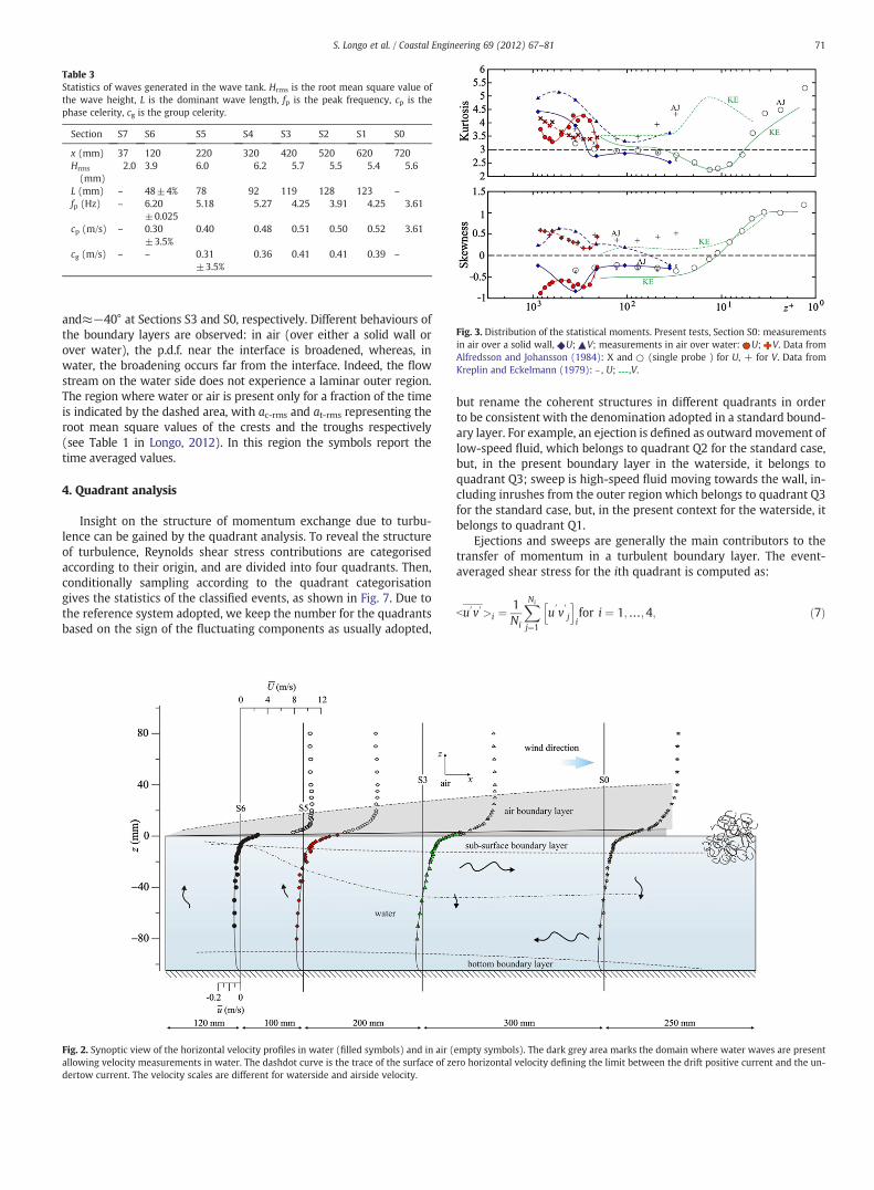
A synoptic description of the mean horizontal velocity profiles isillustrated in Fig. 2. For measurements on the air side, only those ve-locity profiles with their counterparts on the water side are shown.

3. The measured statistics of turbulence

Two important parameters about the variations of the fluctuatingvelocities are the kurtosis and the skewness, shown in Fig. 3 for thehorizontal and vertical velocity components on the air side over asolid wall and over water.

For measurements over a solid wall, the kurtosis, a measure of thepeakedness of the probability density function (p.d.f.), is in good agree-ment with the results in Kreplin and Eckelmann (1979) and Alfredssonand Johansson (1984), which are referred to KE and AJ data respective-ly. Measurements over water lie in a different range with respect to KEand AJ data, but are significantly different from the measurements overa solid wall. The value of the kurtosis is always greater than 3, which isthe value for normal distribution.

The skewness is similar between tests over a solid wall and thoseover water, and follows the trend similar to that obtained by Kreplinand Eckelmann (1979) and Alfredsson and Johansson (1984). As aconsequence of high speed fluid from the outer region, large positiveevents of U occur more frequently than the large negative events of U.The skewness for the horizontal velocity is negative over both solidwall and water, except in the outer region, where the Gaussian prob-ability density distribution is reached. The skewness of the verticalvelocity is always positive except for z+b50, where it becomes nega-tive over a solid wall. Large negative events of V are more frequentthan large positive events of V. Similar results were also obtained byNakagawa et al. (2003), who compared turbulent flows over a flat sur-face and over a surface with sinusoidal shapes of small wavelength.

The results with only the measurements on the water side areshown in Fig. 4. The kurtosis is always larger than 3, with higher valuesfor the vertical velocity.

Skewness is slightly negative for the horizontal velocity and slightlypositive for the vertical velocity except when z+b−300. Beneath theinterface, large positive values of u and large negative values of v areexpected,which are also highly correlated aswill be shown in the quad-rant analysis in Section 4.

For shear flows over a boundary, the edge of the turbulent boundarylayer is not sharp but constantly shifts in a region where turbulence be-comes intermittent, as documented for the first time by Townsend(1948).Wehave verified using the present equipment that the distribu-tion, p(U′), of the probability density of the velocity fluctuation in an

isotropic turbulent flow is Gaussian. A higher kurtosis in the boundarylayer will indicate that most of the variance is due to the infrequent ex-treme deviations hence kurtosis higher than 3 indicates fluctuating tur-bulence called intermittence.

Velocity measurements were also used to calculate the anglebetween the instantaneous vertical fluctuation and the instantaneoushorizontal velocity. At any instant, the compound velocity vector is in-clined at an angle βw ¼ tan−1v′= u þ u′

� �in water and βa ¼

tan−1V ′= U þ U′� �

in air. These values give indications on the directionof themomentum transfer. The normalized probability density distribu-tions of these angles p(β) are shown in Fig. 5 at different levels in theairside and waterside boundary layers. For comparison with data avail-able in the literature, measurements over a solid wall are also shown.The present variations over a solid wall agree with the measurementsgiven by other researchers (e.g. Kreplin and Eckelmann, 1979), withthe maximum and minimum angles expected to be in the rangeβa=±10°. Similar results were also obtained by Antonia et al.(1990) in validating the X hot wire probe they used. They alsofound that the flow geometry was not affected by the Reynolds num-ber Reθ, at least in the range 1360–9630 in their tests.

The data in water show a larger variance of the distribution,and the peak is biased towards negative values. Considering thatthe horizontal velocity is mainly positive (except for z>40 mm due tothe negative return current), the negative bias indicates that the turbu-lence dynamics in water mainly takes place in the fourth quadrant.

The change of angle of peak occurrence with the vertical positionis shown in Fig. 6. The peak is slightly shifted to negative angles inthe range 0° to−5° for airsidemeasurements, but tomuch larger anglesfor the waterside measurements, where the peak reaches≈−30°

Table 1Parameters for mean air velocity profiles at different fetches. The measurements are in air over water. x is the fetch length, U∞ is the asymptotic velocity, u*a is the friction velocity, δis the computed thickness of the boundary layer,Wc is the wake coefficient, Rex=U∞x/νa is the Reynolds number based on x, C is a parameter, δ1 is the displacement thickness and θis the momentum thickness, δ1/θ is the shape factor of the boundary layer, Reθ=U∞θ/νa is the Reynolds number based on momentum thickness, Cf is the friction coefficient.

Section # S7 S6 S5 S4 S3 S2 S1 S0

x (mm) 37 120 220 320 420 520 620 720U∞ (m/s) 10.30 10.50 10.93 10.72 10.74 10.72 10.94 10.92u* a(m/s) 0.39 0.40 0.74 0.71 0.68 0.72 0.63 0.63δ (mm) 3.9 9.4 18.0 19.1 21.2 24.6 28.0 36.2Wc 1.209 0.939 0.350 0.375 0.322 0.323 0.348 0.412Rex 0.252×105 0.834 1.59 2.27 2.99 3.69 4.49 5.21C 8.84 7.76 −3.94 −3.78 −2.97 −4.39 −1.90 −2.95δ1 (mm) 0.8 2.4 4.1 4.6 4.3 5.6 6.3 7.7θ (mm) 0.5 1.4 2.3 2.6 2.8 3.6 3.6 4.4δ1/θ 1.6 1.71 1.78 1.76 1.54 1.56 1.75 1.75Reθ 340 980 1675 1860 2005 2570 2630 3200Cf 1.49×10−3 1.51 4.95 4.72 4.30 4.86 3.54 3.55

Table 2The parameters for the mean water flow velocity profiles at different fetches. The mea-surements are in water. x is the fetch length, u∞ is the asymptotic velocity in the waterstream, u*w is the friction velocity of the water stream, ks is the roughness length,Rex=u∞x/νw is the Reynolds number based on x and on u∞, C is a parameter, δ1 isthe displacement thickness and θ is the momentum thickness, δ1/θ is the shape factorof the boundary layer, Reθ=u∞θ/νw is the Reynolds number based on momentumthickness, Cf is the friction coefficient.

Section # S6 S5 S3 S0

x (mm) 120 220 420 720u∞ (m/s) 0.20 0.33 0.35 0.35u*w (m/s) 0.0095 0.0257 0.0318 0.0257ks (mm) – 7.7 26.7 7.6Rex 24×103 77 147 252C 5.5 −5.57 −8.34 −4.68δ1 (mm) 6.6 7.9 15.9 9.8θ (mm) 3.4 4.5 9.3 4.6δ1/θ 1.94 1.75 1.71 2.13Reθ 1190 1575 3069 920Cf 2.26×10−3 5.39 8.26 5.39



and≈−40° at Sections S3 and S0, respectively. Different behaviours ofthe boundary layers are observed: in air (over either a solid wall orover water), the p.d.f. near the interface is broadened, whereas, inwater, the broadening occurs far from the interface. Indeed, the flowstream on the water side does not experience a laminar outer region.The region where water or air is present only for a fraction of the timeis indicated by the dashed area, with ac-rms and at-rms representing theroot mean square values of the crests and the troughs respectively(see Table 1 in Longo, 2012). In this region the symbols report thetime averaged values.

4. Quadrant analysis

Insight on the structure of momentum exchange due to turbu-lence can be gained by the quadrant analysis. To reveal the structureof turbulence, Reynolds shear stress contributions are categorisedaccording to their origin, and are divided into four quadrants. Then,conditionally sampling according to the quadrant categorisationgives the statistics of the classified events, as shown in Fig. 7. Due tothe reference system adopted, we keep the number for the quadrantsbased on the sign of the fluctuating components as usually adopted,

but rename the coherent structures in different quadrants in orderto be consistent with the denomination adopted in a standard bound-ary layer. For example, an ejection is defined as outwardmovement oflow-speed fluid, which belongs to quadrant Q2 for the standard case,but, in the present boundary layer in the waterside, it belongs toquadrant Q3; sweep is high-speed fluid moving towards the wall, in-cluding inrushes from the outer region which belongs to quadrant Q3for the standard case, but, in the present context for the waterside, itbelongs to quadrant Q1.

Ejections and sweeps are generally the main contributors to thetransfer of momentum in a turbulent boundary layer. The event-averaged shear stress for the ith quadrant is computed as:

bu′v′>i ¼1Ni

XNi

j¼1

u′v′jh i

ifor i ¼ 1;…;4; ð7Þ

Table 3Statistics of waves generated in the wave tank. Hrms is the root mean square value ofthe wave height, L is the dominant wave length, fp is the peak frequency, cp is thephase celerity, cg is the group celerity.

Section S7 S6 S5 S4 S3 S2 S1 S0

x (mm) 37 120 220 320 420 520 620 720Hrms

(mm)2.0 3.9 6.0 6.2 5.7 5.5 5.4 5.6

L (mm) – 48±4% 78 92 119 128 123 –

fp (Hz) – 6.20±0.025

5.18 5.27 4.25 3.91 4.25 3.61

cp (m/s) – 0.30±3.5%

0.40 0.48 0.51 0.50 0.52 3.61

cg (m/s) – – 0.31±3.5%

0.36 0.41 0.41 0.39 –

Fig. 2. Synoptic view of the horizontal velocity profiles in water (filled symbols) and in air (empty symbols). The dark grey area marks the domain where water waves are presentallowing velocity measurements in water. The dashdot curve is the trace of the surface of zero horizontal velocity defining the limit between the drift positive current and the un-dertow current. The velocity scales are different for waterside and airside velocity.

Fig. 3. Distribution of the statistical moments. Present tests, Section S0: measurementsin air over a solid wall, U; V; measurements in air over water: U; V. Data fromAlfredsson and Johansson (1984): X and (single probe ) for U, + for V. Data fromKreplin and Eckelmann (1979): , U; ,V.



where Ni is the number of events in the ith quadrant and j is the cur-rent sample number. The average shear stress for the ith quadrant is

u′v′ i ¼1N

XNi

j¼1

u′v′jh i

ifor i ¼ 1;…;4: ð8Þ

The ratio, Ni/N, is the relative permanence of the events in the i-quadrant, hence

u′v′ i ¼Ni

Nbu′v′>i ð9Þ

Fig. 4. Distribution of the statistical moments, Section S0:measurements in air over a solid wall, U; V; measurements in air over water: U; V; measurements inwater, u; v.

Fig. 5. Probability density distribution of the angle between the instantaneous values of the vertical velocity fluctuation and the horizontal velocity at different distances from theinterfaces, in the airside over a solid wall (left panels), in the airside over water (central panels) and in the waterside (right panels). Measurements in Section S0 in water and in airover a solid wall, in Section S2 in air over water. The vertical scale is different for the three series, the horizontal scale is different for measurements in air over a solid wall.



and the total shear stress is

u′v′ ¼X4i¼1

u′v′ i: ð10Þ

It is of interest to restrict the analysis to values above a fixedthreshold. These values indicate the presence of coherent structurescarrying a significant momentum in the boundary layer. The thresh-old is usually defined as:

u′v′�� > Hu′

rmsv′rms ð11Þ

where H is a threshold. The concentration of the ith quadrant for afixed threshold level is

C iH ¼ 1

N

XNj¼1

ϕiH;j; ð12Þ

where

ϕiH; j ¼

1if u′v′��

j> Hu′

rmsv′rms and belongs to the i� quadrant

0 otherwise

(ð13Þ

We can also consider the phasic-averaged Reynolds stress for theith quadrant:

u′v′̂

� �i

H¼

PNj¼1

u′v′� �

jϕiH; j

PNj¼1

ϕiH; j

; ð14Þ

and the time-averaged Reynolds stress for the ith quadrant:

u′v′� �i

H¼ 1

N

XNj¼1

u′v′� �

jϕiH;j ¼ C i

H u′v′̂

� �i

Hð15Þ

also expressed in the non-dimensional form as stress fraction:

SiH ¼ u′v′

� �iHu′v′ : ð16Þ

Furthermore,

S10 þ S20 þ S30 þ S40 ¼ 1: ð17Þ

The conditional averages are strictly related to the joint probabilitydensity function of thefluctuating velocities. In Fig. 8, thefluctuating ve-locities' p.d.f. for measurements in water is shown at three levels. Thecontours, with a constant interval of each 10%, are elliptic with themajor axis along the bisector of quadrants Q2 and Q4 at the interface

Fig. 6. Measurements in air over water and in water. Angle of peak occurrence of probability density distribution of the angle between the instantaneous values of vertical velocityfluctuations and horizontal velocity. : Section S0, : Section S3. The empty symbols refer to measurements in water above the still water level. ac-rms, at-rms is the root meansquare value of the crests, of the troughs.

Fig. 7. Quadrant decomposition of the fluctuating components of velocity.



and at levels beneath the interface, indicating that the fluctuations tendto inhibit each other in the first and the third quadrants. For measure-ments above the still water level, the correlation is weaker, and con-tours seem to be uniformly distributed.

Similar p.d.f. on the air side has been observed, as reported inFig. 15 of Longo and Losada (2012). This shows that, near the edge ofthe airside boundary layer, turbulence appears to be isotropic, whereas,near the interface, it becomes elliptic with sweeps dominant.

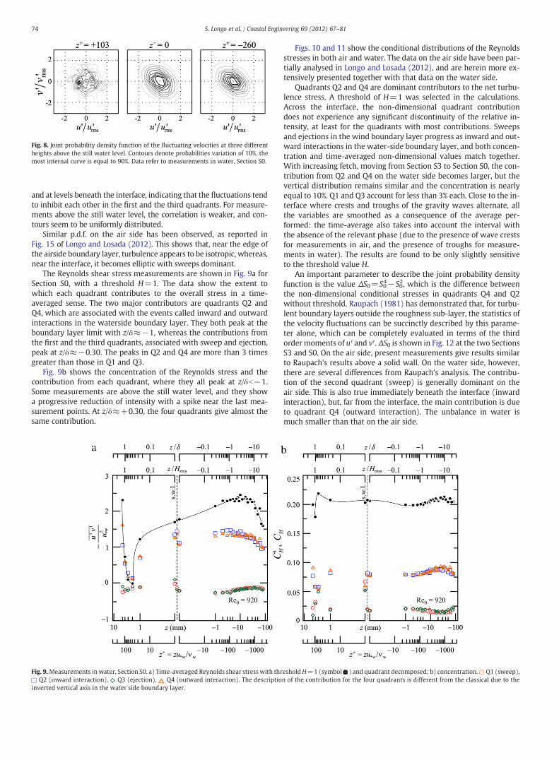
The Reynolds shear stress measurements are shown in Fig. 9a forSection S0, with a threshold H=1. The data show the extent towhich each quadrant contributes to the overall stress in a time-averaged sense. The two major contributors are quadrants Q2 andQ4, which are associated with the events called inward and outwardinteractions in the waterside boundary layer. They both peak at theboundary layer limit with z/δ≈−1, whereas the contributions fromthe first and the third quadrants, associated with sweep and ejection,peak at z/δ≈−0.30. The peaks in Q2 and Q4 are more than 3 timesgreater than those in Q1 and Q3.

Fig. 9b shows the concentration of the Reynolds stress and thecontribution from each quadrant, where they all peak at z/δb−1.Some measurements are above the still water level, and they showa progressive reduction of intensity with a spike near the last mea-surement points. At z/δ≈+0.30, the four quadrants give almost thesame contribution.

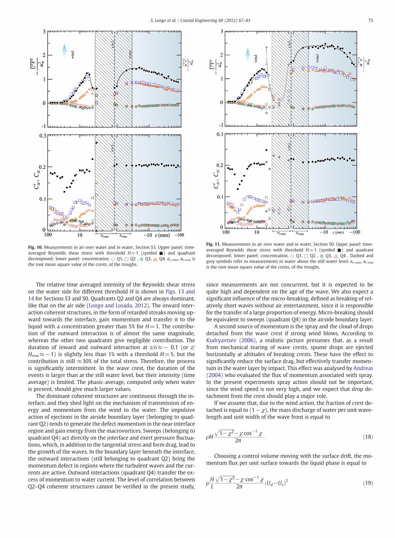
Figs. 10 and 11 show the conditional distributions of the Reynoldsstresses in both air and water. The data on the air side have been par-tially analysed in Longo and Losada (2012), and are herein more ex-tensively presented together with that data on the water side.

Quadrants Q2 and Q4 are dominant contributors to the net turbu-lence stress. A threshold of H=1 was selected in the calculations.Across the interface, the non-dimensional quadrant contributiondoes not experience any significant discontinuity of the relative in-tensity, at least for the quadrants with most contributions. Sweepsand ejections in the wind boundary layer progress as inward and out-ward interactions in the water-side boundary layer, and both concen-tration and time-averaged non-dimensional values match together.With increasing fetch, moving from Section S3 to Section S0, the con-tribution from Q2 and Q4 on the water side becomes larger, but thevertical distribution remains similar and the concentration is nearlyequal to 10%. Q1 and Q3 account for less than 3% each. Close to the in-terface where crests and troughs of the gravity waves alternate, allthe variables are smoothed as a consequence of the average per-formed: the time-average also takes into account the interval withthe absence of the relevant phase (due to the presence of wave crestsfor measurements in air, and the presence of troughs for measure-ments in water). The results are found to be only slightly sensitiveto the threshold value H.

An important parameter to describe the joint probability densityfunction is the value ΔS0=S0

4−S02, which is the difference between

the non-dimensional conditional stresses in quadrants Q4 and Q2without threshold. Raupach (1981) has demonstrated that, for turbu-lent boundary layers outside the roughness sub-layer, the statistics ofthe velocity fluctuations can be succinctly described by this parame-ter alone, which can be completely evaluated in terms of the thirdorder moments of u′ and v′. ΔS0 is shown in Fig. 12 at the two SectionsS3 and S0. On the air side, present measurements give results similarto Raupach's results above a solid wall. On the water side, however,there are several differences from Raupach's analysis. The contribu-tion of the second quadrant (sweep) is generally dominant on theair side. This is also true immediately beneath the interface (inwardinteraction), but, far from the interface, the main contribution is dueto quadrant Q4 (outward interaction). The unbalance in water ismuch smaller than that on the air side.

Fig. 8. Joint probability density function of the fluctuating velocities at three differentheights above the still water level. Contours denote probabilities variation of 10%, themost internal curve is equal to 90%. Data refer to measurements in water, Section S0.

Fig. 9.Measurements in water, Section S0. a) Time-averaged Reynolds shear stress with thresholdH=1 (symbol ) and quadrant decomposed; b) concentration. Q1 (sweep),Q2 (inward interaction), Q3 (ejection), Q4 (outward interaction). The description of the contribution for the four quadrants is different from the classical due to the

inverted vertical axis in the water side boundary layer.



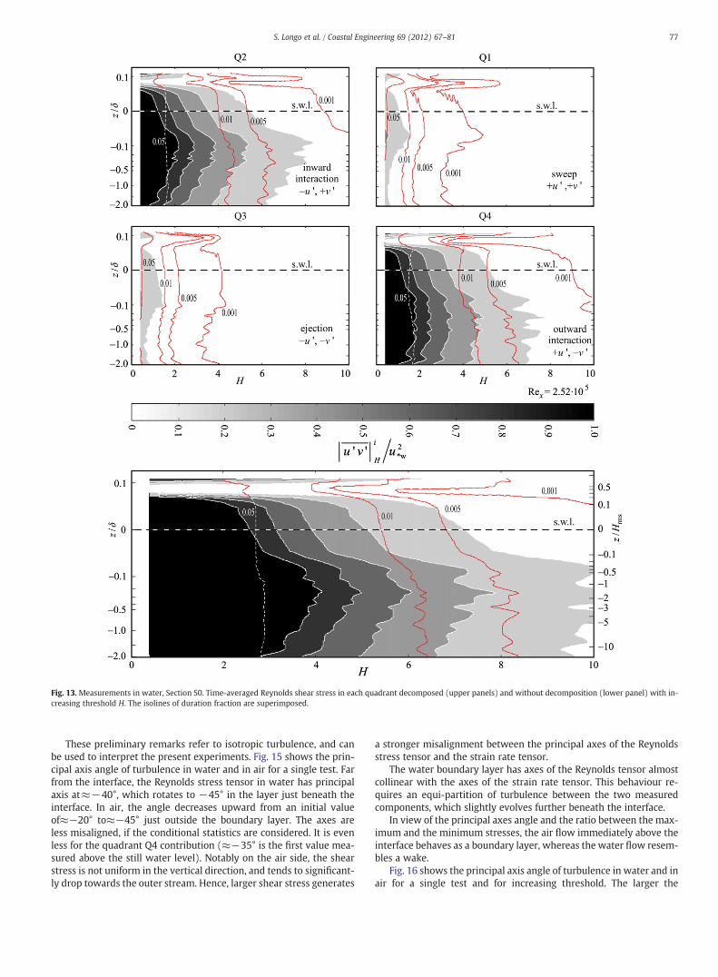
The relative time averaged intensity of the Reynolds shear stresson the water side for different threshold H is shown in Figs. 13 and14 for Sections S3 and S0. Quadrants Q2 and Q4 are always dominant,like that on the air side (Longo and Losada, 2012). The inward inter-action coherent structures, in the form of retarded streaks moving up-ward towards the interface, gain momentum and transfer it to theliquid with a concentration greater than 5% for H=1. The contribu-tion of the outward interaction is of almost the same magnitude,whereas the other two quadrants give negligible contribution. Theduration of inward and outward interaction at z/δ≈− 0.1 (or z/Hrms≈−1) is slightly less than 1% with a threshold H=5, but thecontribution is still ≈30% of the total stress. Therefore, the processis significantly intermittent. In the wave crest, the duration of theevents is larger than at the still water level, but their intensity (timeaverage) is limited. The phasic-average, computed only when wateris present, should give much larger values.

The dominant coherent structures are continuous through the in-terface, and they shed light on the mechanism of transmission of en-ergy and momentum from the wind to the water. The impulsiveaction of ejections in the airside boundary layer (belonging to quad-rant Q2) tends to generate the defect momentum in the near interfaceregion and gain energy from the macrovortices. Sweeps (belonging toquadrant Q4) act directly on the interface and exert pressure fluctua-tions, which, in addition to the tangential stress and form drag, lead tothe growth of the waves. In the boundary layer beneath the interface,the outward interactions (still belonging to quadrant Q2) bring themomentum defect in regions where the turbulent waves and the cur-rents are active. Outward interactions (quadrant Q4) transfer the ex-cess of momentum to water current. The level of correlation betweenQ2–Q4 coherent structures cannot be verified in the present study,

since measurements are not concurrent, but it is expected to bequite high and dependent on the age of the wave. We also expect asignificant influence of the micro-breaking, defined as breaking of rel-atively short waves without air entertainment, since it is responsiblefor the transfer of a large proportion of energy. Micro-breaking shouldbe equivalent to sweeps (quadrant Q4) in the airside boundary layer.

A second source of momentum is the spray and the cloud of dropsdetached from the wave crest if strong wind blows. According toKudryavtsev (2006), a realistic picture presumes that, as a resultfrom mechanical tearing of wave crests, spume drops are ejectedhorizontally at altitudes of breaking crests. These have the effect tosignificantly reduce the surface drag, but effectively transfer momen-tum in the water layer by impact. This effect was analysed by Andreas(2004) who evaluated the flux of momentum associated with spray.In the present experiments spray action should not be important,since the wind speed is not very high, and we expect that drop de-tachment from the crest should play a major role.

If we assume that, due to the wind action, the fraction of crest de-tached is equal to (1−χ), the mass discharge of water per unit wave-length and unit width of the wave front is equal to

ρH

ffiffiffiffiffiffiffiffiffiffiffiffiffiffi1−χ2

p−χ cos−1χ2π

: ð18Þ

Choosing a control volume moving with the surface drift, the mo-mentum flux per unit surface towards the liquid phase is equal to

ρHL


p−χ cos−1χ2π

Ud−Usð Þ2 ð19Þ

Fig. 10. Measurements in air over water and in water, Section S3. Upper panel: time-averaged Reynolds shear stress with threshold H=1 (symbol ) and quadrantdecomposed; lower panel: concentration. Q1, Q2 , Q3, Q4. ac-rms, at-rms isthe root mean square value of the crests, of the troughs.

Fig. 11. Measurements in air over water and in water, Section S0. Upper panel: time-averaged Reynolds shear stress with threshold H=1 (symbol ) and quadrantdecomposed; lower panel: concentration. Q1, Q2 , Q3, Q4 . Dashed andgrey symbols refer to measurements in water above the still water level. ac-rms, at-rms

is the root mean square value of the crests, of the troughs.



where Ud is the velocity of the detached drops when impinging on theliquid surface. The non-dimensional form results:

τmb

ρu2�w

¼ HL


p−χ cos−1χ2π

Ud−Us

u�w

� �2: ð20Þ

Considering the data in Section S0 and assuming that the velocityof the detached drops is equal to the phase celerity and that the re-duction of the wave crest due to spray and droplet generation isequal to 10%, substituting in Eq. (20) results in the following stressper unit mass density

τmb ¼ 5:4� 10−3

0:123

ffiffiffiffiffiffiffiffiffiffiffiffiffiffiffiffiffi1−0:92

p−0:9 cos−10:92π

0:52−0:55� 0:630:0257

� �2≈0:01u2

�w

ð21ÞIt is a small value, similar to that obtained by the Andreas (2004)

model for spray. A strong increment is obtained by assuming that thedroplets, once detached, are accelerated by the fast wind stream. In-deed they can easily reach the wind speed before falling if their radiusis sufficiently small. If their velocity at impact is equal to 1 m/s, thecontribution becomes τmb≈0.14u*w2 , which starts to be significant.If Ud=2 m/s, then τmb≈0.86u*w2 , which is definitely significant. Theforce necessary to accelerate the droplets is already included in thefriction of the wind, and does not change the drag. For small droplets,the acceleration due to the wind can be much stronger, so the fastdroplets can transfer a larger amount of momentum, even thoughthe violent aeration vaporizes part of the detached mass.

5. Reynolds stress tensor's principal axes

The interaction between the mean motion and the fluctuating ve-locity can be analysed observing the Reynolds stress tensor. The sim-plest experiment concerning the response of the principal axes of theReynolds stress tensor to the external flow field is the action of a con-stant pure plane strain on an initially isotropic turbulence(Townsend, 1954; Tucker and Reynolds, 1968). In that case, the prin-cipal axes of the Reynolds stress tensor are those of the mean rate ofstrain, and the turbulent motion appears as ‘oriented’ by the strainfield. If the strain field changes, the axes of the Reynolds stress tensorhave a tendency to be reoriented along the axes of the new strain,with a delay related to a relaxation time of the order of the timescale of the imposed strain. If the strain tensor reduces to a pureshear stress, several experiments (e.g. Harris et al., 1977) show that,for isotropic turbulence, the principal axes of the Reynolds stress

tensor are not aligned with those of the strain, which is a conse-quence of the mean rotation. In Harris et al. (1977) experiments, asudden variation of a pure strain is applied to grid-generated turbu-lence. These results should be midway between those with constantuniform strains and those with pure uniform shears. In fact, a con-stant shear situation can be composed by superposing a pure planestrain on a mean rotation. Hence, the action of the constant shear isequivalent to one of a pure plane strain, the principal axes of whichinstantaneously rotate around an axis perpendicular to the plane ofthe strain. The characteristic time of the mean rotation and the asso-ciated strain is twice the characteristic time of the shearing, i.e. the re-laxation time of re-orientation of the Reynolds stress tensor. Hence, inshearing, the principal axes of the Reynolds stress tensor cannot bealigned with those of the associated strain, which make a 45° anglewith the direction of the flow, even though the tendency is towardsa complete re-alignment. The general picture shows that the principalaxes of the two tensors are not collinear. The co-linearity is closely re-lated to a common model of turbulence, which relates the Reynoldsstress tensor to the strain rate tensor in a linear Newtonian fashion:

−u′iu

′j þ

23κδij ¼ νt Sij ð22Þ

where κ is the turbulent kinetic energy, νt is the eddy viscosity and Sijis the strain rate tensor. The over bar indicates the correlation. This isan isotropic algebraic constitutive relation that works fairly well forwakes but less well for many other flows. The orientation found inthe boundary layer and channel flow is (see Champagne et al.,1970) ασ≈−20° to −25° and 70° to 65°, while that in the wake isασ≈40° to 50° and −50° to −40°. In both cases, the principal axesof the strain rate tensor are αD=±45°. Also, the ratio of the maxi-mum–minimum stresses is the characteristic of specific flows. Thetwo principal stresses in the x–z plane are

σa;b ¼ u′u′ þ v′v′

2�

ffiffiffiffiffiffiffiffiffiffiffiffiffiffiffiffiffiffiffiffiffiffiffiffiffiffiffiffiffiffiffiffiffiffiffiffiffiffiffiffiffiffiffiffiffiffiffiffiffiffiffiffiffiu′u′−v′v′

2

!2

þ u′v′� �2vuut ð23Þ

and their ratio is (see Champagne et al., 1970):

boundary layer : σa=σb ¼ 3 to 4channel : σa=σb ¼ 3 to 5

plane wake : σa=σb ¼ 2 to 6g ð24Þ

The present experiments results in σa/σb=1.5 to 3 on the waterside and σa/σb=3 to 4 on the air side (not shown).

Fig. 12. The differenceΔS0 betweenQ4 andQ2 stress contributions for the two Sections S3 and S0: measurements over a solidwall;♦measurements in air overwater; measurementsin water. Grey symbols refer to measurements in water above the still water level. ac-rms, at-rms is the root mean square value of the crests, of the troughs.



These preliminary remarks refer to isotropic turbulence, and canbe used to interpret the present experiments. Fig. 15 shows the prin-cipal axis angle of turbulence in water and in air for a single test. Farfrom the interface, the Reynolds stress tensor in water has principalaxis at≈−40°, which rotates to −45° in the layer just beneath theinterface. In air, the angle decreases upward from an initial valueof≈−20° to≈−45° just outside the boundary layer. The axes areless misaligned, if the conditional statistics are considered. It is evenless for the quadrant Q4 contribution (≈−35° is the first value mea-sured above the still water level). Notably on the air side, the shearstress is not uniform in the vertical direction, and tends to significant-ly drop towards the outer stream. Hence, larger shear stress generates

a stronger misalignment between the principal axes of the Reynoldsstress tensor and the strain rate tensor.

The water boundary layer has axes of the Reynolds tensor almostcollinear with the axes of the strain rate tensor. This behaviour re-quires an equi-partition of turbulence between the two measuredcomponents, which slightly evolves further beneath the interface.

In view of the principal axes angle and the ratio between the max-imum and the minimum stresses, the air flow immediately above theinterface behaves as a boundary layer, whereas the water flow resem-bles a wake.

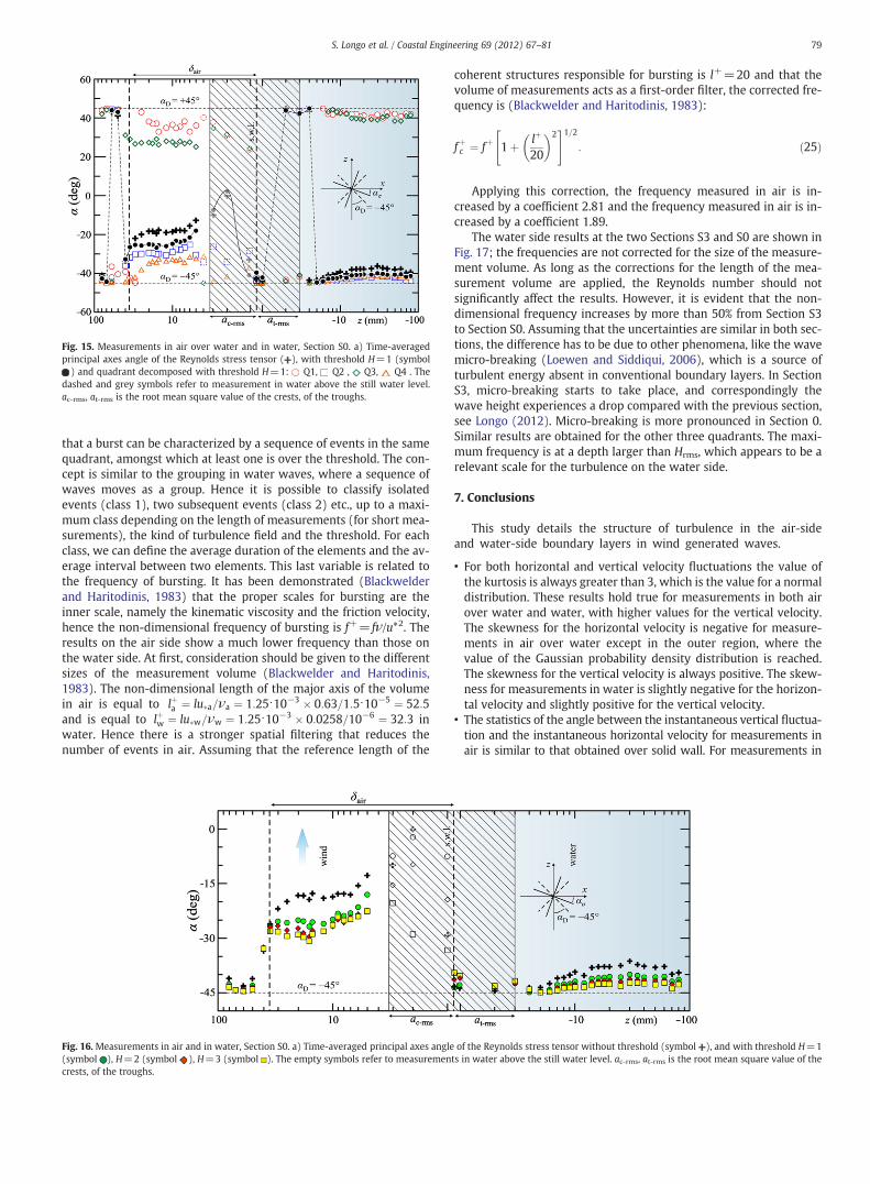
Fig. 16 shows the principal axis angle of turbulence in water and inair for a single test and for increasing threshold. The larger the

Fig. 13. Measurements in water, Section S0. Time-averaged Reynolds shear stress in each quadrant decomposed (upper panels) and without decomposition (lower panel) with in-creasing threshold H. The isolines of duration fraction are superimposed.



threshold the lower is the angle misalignment, with an asymptoticvalue which is different from zero.

6. A new description of the burst

Intensive studies of turbulent boundary layers have led to the rec-ognition of coherent structures. This is manifested by formationstreak patterns, lifting and oscillation of low-speed fluid, abrupt ejec-tion of this low-speed fluid outward (this sequence of events is col-lectively known as bursting), and the strong motion of the outer,faster moving fluid towards the wall (sweep). Bursting is often

described as a highly intermittent, explosive event. Intermittency isoften with respect to time, however several experiments and numer-ical investigations (see Robinson, 1991, for a review) show that tur-bulent structures are more intermittent in space than in time. Oncea coherent structure with a high level of turbulence intensity is pro-duced, it moves in the fluid, presenting as a strong intermittentevent for measurement at a fixed point. We expect that the probabil-ity of two subsequent strong events (e.g. u′v′ in the same quadrantover a threshold) as recorded by a fixed probe is generally high ifthere are coherent structures moving in the fluid. In order to analysethis aspect, a different description of burst is herein used. We assume

Fig. 14. Measurements in water, Section S3. Time-averaged Reynolds shear stress in each quadrant decomposed (upper panels) and without decomposition (lower panel) with in-creasing threshold H. The isolines of duration fraction are superimposed.



that a burst can be characterized by a sequence of events in the samequadrant, amongst which at least one is over the threshold. The con-cept is similar to the grouping in water waves, where a sequence ofwaves moves as a group. Hence it is possible to classify isolatedevents (class 1), two subsequent events (class 2) etc., up to a maxi-mum class depending on the length of measurements (for short mea-surements), the kind of turbulence field and the threshold. For eachclass, we can define the average duration of the elements and the av-erage interval between two elements. This last variable is related tothe frequency of bursting. It has been demonstrated (Blackwelderand Haritodinis, 1983) that the proper scales for bursting are theinner scale, namely the kinematic viscosity and the friction velocity,hence the non-dimensional frequency of bursting is f+= fν/u*2. Theresults on the air side show a much lower frequency than those onthe water side. At first, consideration should be given to the differentsizes of the measurement volume (Blackwelder and Haritodinis,1983). The non-dimensional length of the major axis of the volumein air is equal to lþa ¼ lu�a=νa ¼ 1:25⋅10−3 � 0:63=1:5⋅10−5 ¼ 52:5and is equal to lþw ¼ lu�w=νw ¼ 1:25⋅10−3 � 0:0258=10−6 ¼ 32:3 inwater. Hence there is a stronger spatial filtering that reduces thenumber of events in air. Assuming that the reference length of the

coherent structures responsible for bursting is l+=20 and that thevolume of measurements acts as a first-order filter, the corrected fre-quency is (Blackwelder and Haritodinis, 1983):

fþc ¼ fþ 1þ lþ

20

� �2" #1=2

: ð25Þ

Applying this correction, the frequency measured in air is in-creased by a coefficient 2.81 and the frequency measured in air is in-creased by a coefficient 1.89.

The water side results at the two Sections S3 and S0 are shown inFig. 17; the frequencies are not corrected for the size of the measure-ment volume. As long as the corrections for the length of the mea-surement volume are applied, the Reynolds number should notsignificantly affect the results. However, it is evident that the non-dimensional frequency increases by more than 50% from Section S3to Section S0. Assuming that the uncertainties are similar in both sec-tions, the difference has to be due to other phenomena, like the wavemicro-breaking (Loewen and Siddiqui, 2006), which is a source ofturbulent energy absent in conventional boundary layers. In SectionS3, micro‐breaking starts to take place, and correspondingly thewave height experiences a drop compared with the previous section,see Longo (2012). Micro-breaking is more pronounced in Section 0.Similar results are obtained for the other three quadrants. The maxi-mum frequency is at a depth larger than Hrms, which appears to be arelevant scale for the turbulence on the water side.

7. Conclusions

This study details the structure of turbulence in the air-sideand water-side boundary layers in wind generated waves.

• For both horizontal and vertical velocity fluctuations the value ofthe kurtosis is always greater than 3, which is the value for a normaldistribution. These results hold true for measurements in both airover water and water, with higher values for the vertical velocity.The skewness for the horizontal velocity is negative for measure-ments in air over water except in the outer region, where thevalue of the Gaussian probability density distribution is reached.The skewness for the vertical velocity is always positive. The skew-ness for measurements in water is slightly negative for the horizon-tal velocity and slightly positive for the vertical velocity.

• The statistics of the angle between the instantaneous vertical fluctua-tion and the instantaneous horizontal velocity for measurements inair is similar to that obtained over solid wall. For measurements in

Fig. 15. Measurements in air over water and in water, Section S0. a) Time-averagedprincipal axes angle of the Reynolds stress tensor ( ), with threshold H=1 (symbol) and quadrant decomposed with threshold H=1: Q1, Q2 , Q3, Q4 . The

dashed and grey symbols refer to measurement in water above the still water level.ac-rms, at-rms is the root mean square value of the crests, of the troughs.

Fig. 16. Measurements in air and in water, Section S0. a) Time-averaged principal axes angle of the Reynolds stress tensor without threshold (symbol ), and with threshold H=1(symbol ), H=2 (symbol ), H=3 (symbol ). The empty symbols refer to measurements in water above the still water level. ac-rms, at-rms is the root mean square value of thecrests, of the troughs.



water, it shows a large variance and the peak is biased towards nega-tive angles.

• In the quadrants analysis, the contribution of quadrants Q2 and Q4is dominant on both air side and water side. The nomenclature ofthe related coherent structures is sweeps and ejections on the airside, and becomes inward and outward interactions on the waterside. The non-dimensional relative contributions and the concen-tration match fairly well near the interface. Sweeps in the air side(belonging to quadrant Q4) act directly on the interface and exertpressure fluctuations, which, in addition to the tangential stressand form drag, lead to the growth of the waves.

• The water drops detached from the crest and accelerated by thewind can play a major role in transferring momentum and in en-hancing the turbulence level in the water side.

• On the air side, the Reynolds stress tensor's principal axes are notcollinear with the strain rate tensor, and show an angleασ≈−20° to−25°, while the angle of the strain rate tensor isαD=±45°. This is similar to the orientation found in boundarylayer and channel flows. On the water side, the angle isασ≈−40° to−45°, similar to the angle found in wakes, and theangle of the strain rate tensor is stillαD=±45°. The ratio betweenthe maximum and the minimum principal stresses is σa/σb=3 to 4on the air side and σa/σb=1.5 to 3 on the water side. In this respect,the air side flow behaves like a classical boundary layer while thewater side flow resembles a wake.

• The frequency of bursting on the water side shows a strong incre-ment from Section S3 to Section S0, which the increase of fetch. Itis attributed to micro-breaking effects, which are expected to bemore important at larger fetches.

8. List of the symbols

…― time average operator…̃ oscillating term operator…ˆ phasic average operatorαD angle of the strain rate tensor principal axesασ angle of the Reynolds stress tensor principal axesβw, βa, βp angle in water, in air, angle of peak occurrenceδ boundary layer thicknessδ1 displacement thickness of the boundary layerδ1/θ shape factor of the boundary layerρ mass densityθ thickness of the boundary layer based on momentumκ turbulent kinetic energyνa, νw kinematic fluid viscosity of the air, of the waterσa,b maximum, minimum principal stressτmb stress due to spray and detached dropsac-rms, at-rms

root mean square value of the crests, of the troughsC concentration, coefficientCf friction coefficientcp, cg celerity of phase, of groupf+, fc, fc+ non‐dimensional frequency (internal scales), corrected fre-

quency, non-dimensional corrected frequency (internalscales)

fp peak frequencyH wave height, threshold coefficient

Fig. 17. Non‐dimensional frequency of bursts event in Section S3 (upper panel) and Section S0 (lower panel), quadrant Q2. all bursts; bursts of length 1; bursts of length 2;bursts of length 3; bursts of length 4; bursts of length 5.



Hrms root mean square wave heightk von Karman constantks roughness lengthl, l+ length, non-dimensional length (internal scales)L wave lengthp.d.f., p(…) probability density functionRe, Rex, Reθ Reynolds number, based on the abscissa x, on momen-

tum thicknessSij tensor of strain rateSHi non‐dimensional stress for the ith quadrant with threshold

Hs.w.l. still water levelt timeU∞ asymptotic wind velocityUs drift velocityU, V streamwise, vertical wind velocityU′, V′ streamwise, vertical fluctuating wind velocityUd velocity of the detached dropsu∞ asymptotic water velocityu, v streamwise, vertical water velocityu′, v′ streamwise, vertical fluctuating water velocityu′rms, v′rms

root mean square streamwise, vertical fluctuating water velocityu*a friction velocity in the air boundary layeru*w friction velocity in the water boundary layerW(…) wake functionWc wake coefficientx, z spatial co-ordinatesz+ non‐dimensional vertical coordinate (internal scales)

Acknowledgements

The experimental data presented herein were obtained during theauthor's sabbatical leave at CEAMA, Grupo de Dinámica de FlujosAmbientales, University of Granada, Spain, kindly hosted by MiguelA. Losada. Financial support from CEAMA is gratefully acknowledged.Special thanks are given to Simona Bramato and Christian Mans, whoprovided great help with experiments.

References

Alfredsson, R.J., Johansson, A.V., 1984. On the detection of turbulence-generatingevents. Journal of Fluid Mechanics 139 (1), 325–345.

Andreas, E.L., 2004. Spray stress revisited. Journal of Physical Oceanography 34,1429–1440.

Antonia, R.A., Bisset, D.K., Browne, L.W.B., 1990. Effect of Reynolds number on the to-pology of the organized motion in a turbulent boundary layer. Journal of Fluid Me-chanics 213 (1), 267–286.

Blackwelder, R.F., Haritodinis, J.H., 1983. Scaling of the bursting frequency in turbulentboundary layers. Journal of Fluid Mechanics 132, 87–103.

Brocchini, M., Peregrine, D.H., 2001. The dynamics of strong turbulence at free surfaces.Part 1. Description. Journal of Fluid Mechanics 449, 225–254.

Camussi, R., Gui, G., 1997. Orthonormal wavelet decomposition of turbulent flows: in-termittency and coherent structures. Journal of Fluid Mechanics 348, 177–199.

Champagne, F.H., Harris, V.G., Corrsin, S., 1970. Experiments on nearly homogeneousturbulent shear flow. Journal of Fluid Mechanics 41 (01), 81–139.

Chiapponi, L., Longo, S., Bramato, S., Mans, C., Losada, A.M., 2011. Free-surface turbu-lence, wind generated waves: laboratory data. Technical Report on ExperimentalActivity in Granada, University of Parma (Italy). CEAMA, Granada, Spain.

Donelan, M.A., 1998. Air–water exchange processes. In: Imberger, J. (Ed.), Physical Pro-cesses in Lakes and Oceans. : Coast. Estuar. Stud., 54. Am. Geophys. Union, Wash-ington, DC, pp. 19–36.

Foster, R.C., Vianey, F., Drobinski, P., Carlotti, P., 2006. Near-surface coherent structuresand the vertical momentum flux in a large-eddy simulation of the neutrally-stratified boundary layer. Boundary Layer Meteorology 120, 229–255.

Harris, V.G., Graham, J.A.H., Corrsin, S., 1977. Further experiments in nearly homoge-neous turbulent shear flow. Journal of Fluid Mechanics 81 (4), 657–687.

Hunt, J.C.R., Stretch, D.D., Belcher, S.E., 2011. Viscous coupling of shear-free turbulenceacross nearly flat fluid interfaces. Journal of Fluid Mechanics 671 (iii), 96–120.

Kreplin, H., Eckelmann, H., 1979. Behavior of the three fluctuating velocity componentsin the wall region of a turbulent channel flow. Physics of Fluids 22 (7), 1233–1239.

Krostad, P.Å., Antonia, R.A., 1999. Surface roughness effects in turbulent boundarylayers. Experiments in Fluids 27, 450–460.

Kudryavtsev, V.N., 2006. On the effect of sea drops on the atmospheric boundary layer.Journal of Geophysical Research 111, C07020.

Loewen, M.R., Siddiqui, M.H.K., 2006. Detecting microscale breaking waves. Measure-ment Science and Technology 17, 771–780.

Longo, S., 2012. Wind-generated water waves in a wind tunnel: free surface statisticswind friction and mean air flow properties. Coastal Engineering 61, 27–41.

Longo, S., Losada, M.A., 2012. Turbulent structure of air flow over wind-induced gravitywaves. Experiments in Fluids, http://dx.doi.org/10.1007/s00348-012-1294-4 (pub-lished online since 30.3.2012).

Longo, S., Liang, D., Chiapponi, L., Aguilera Jiménez, L., 2012. Turbulent flow structure inexperimental laboratory wind-generated gravity waves. Coastal Engineering 64,1–15.

Nakagawa, S., Na, Y., Hanratty, T.J., 2003. Influence of a wavy boundary on turbulence. I.Highly rough surface. Experiments in Fluids 35, 422–436.

Nolan, K.P., Walsh, E.J., McEligot, D.M., 2010. Quadrant analysis of a transitional bound-ary layer subject to free-stream turbulence. Journal of Fluid Mechanics 658,310–335.

Raupach, M.R., 1981. Conditional statistics of Reynolds stress in rough-wall andsmooth-wall turbulent boundary layers. Journal of Fluid Mechanics 108, 363–382.

Robinson, S.K., 1991. Coherent motions in the turbulent boundary layer. Annual Re-view in Fluid Mechanics 23, 601–639.

Townsend, A.A., 1948. Local isotropy in the turbulent wake of a cylinder. AustralianJournal of Scientific Research, Series A: Physical Sciences 1, 161–174.

Townsend, A.A., 1954. The uniform distortion of homogeneous turbulence. QuarterlyJournal of Mechanics and Applied Mathematics 7 (1), 104–127.

Tucker, J., Reynolds, A.J., 1968. The distortion of turbulence by irrotational plane strain.Journal of Fluid Mechanics 32, 657–673.


coastal engineering - unipr.itslongo/publications/longo_et_al_ce_2012b.pdf · coastal engineering...

Documents