coercive contract enforcement: law and the labor...
TRANSCRIPT

Coercive Contract Enforcement: Law and the LaborMarket in 19th Century Industrial Britain
Suresh Naidu and Noam Yuchtman∗
February 13, 2012
Abstract
British Master and Servant law made employee contract breach a criminal offenseuntil 1875. We develop a contracting model generating equilibrium contract breach andprosecutions, then exploit exogenous changes in output prices to examine the effectsof labor demand shocks on prosecutions. Positive shocks in the textile, iron, andcoal industries increased prosecutions. Following the abolition of criminal sanctions,wages differentially rose in counties that had experienced more prosecutions, and wagesresponded more to labor demand shocks. Coercive contract enforcement was appliedin industrial Britain; restricted mobility allowed workers to commit to risk-sharingcontracts with lower, but less volatile, wages.
JEL codes: J41, K31, N33, N43.
∗Naidu: Columbia University; contact: [email protected]. Yuchtman: Haas School of Business,UC-Berkeley; contact: [email protected]. We thank Ryan Bubb, Davide Cantoni, Greg Clark,Melissa Dell, Oeindrila Dube, Stan Engerman, James Fenske, Camilo Garcia, Claudia Goldin, Larry Katz,Peter Lindert, James Robinson, and participants in the 2009 all-UC Economic History Conference andthe Harvard Economic History Workshop for their comments. Remeike Forbes provided excellent researchassistance.

Economists and economic historians often draw a bright line between free and forced
labor. Forced labor is typically studied in the context of agricultural, preindustrial economies;
free labor is seen as a crucial component of economic modernization and development, and
is implicitly assumed in contemporary models of labor markets. However, “intermediate”
labor market institutions – between free and forced labor – have been common throughout
history.
Indeed, one sees shades of coercion in the world’s first industrial economy, in 19th century
Britain. Until 1875, when it was repealed, Master and Servant law gave employers the ability
to criminally (as opposed to civilly) prosecute and severely punish a majority of employees
across industries for breach of contract in Great Britain.1 Nor was this law left to rot in
the books: there were over 10,000 Master and Servant prosecutions per year between 1858
and 1875 – more prosecutions than for petty larceny – and these occurred across Britain,
especially in industrial northern England (see Figure 1, panels A and B).2
Our work theoretically and empirically studies the effects of Master and Servant law on
contracting and wages in 19th century Britain. Guided by a model of contractual risk-sharing
with limited commitment, which generates equilibrium contract breach and criminal prose-
cutions, this paper examines the economic causes and consequences of criminal prosecutions
under Master and Servant law. We use a panel dataset on prosecutions of workers in English
and Welsh districts, and exogenous, sector-specific labor demand shocks, to estimate the
response of prosecutions for breach of contract to changing labor demand.3 We find that
criminal prosecution of workers, rather than being a vestige of medieval common law, was ac-
tively used in the leading industrial sectors of 19th century Britain. In addition, we examine
1Master and Servant law covered employees in a wide variety of sectors, from farm workers, to coalminers, to textile mill workers, to shoemakers, and beyond (although white collar workers and managerswere excluded). See Appendix 1A, and especially Table A1. The term “Servant” thus had far broaderapplication in the law than in contemporary parlance.
2Statistics come from Judicial Statistics, England and Wales. To place these prosecution figures intocontext, Judicial Statistics, England and Wales reports 14,353 Master and Servant cases and 11,986 casesof larceny of less than 5 shillings in 1875.
3The districts are more disaggregated than British counties. Our dataset contains 52 English and Welshcounties and a total of 219 districts.
1

0
2000
4000
6000
8000
10000
12000
14000
16000
18000
20000
Nu
mb
er o
f p
rose
cu
tion
s
M&S
V&B
Year
Panel B: Distribution of Master and Servant Prosecutions
Across British Counties
0
1
2
3
4
5
6
7
8
0.3
0.35
0.4
0.45
0.5
0.55
0.6
0.65
0.7
Un
em
plo
ym
en
t rate
Prosecu
tio
ns p
er 1
000
mean prosecutions
unemployment
Year
Panel A: Total Prosecutions per Year
Panel C: Unemployment and Prosecutions per Capita per Year
Figure 1: Panel A, on the top left, shows the total number of Master and Servant prosecutions per year, with the number of vagrancy and beggingprosecutions also plotted. Panel B, on the right, shows the average number of Master and Servant prosecutions per 1,000 inhabitants of eachcounty, per year, over the period 1858-1875. Panel C, on the bottom left, shows the average number of Master and Servant prosecutions per 1,000inhabitants of each county, across England and Wales, for each year over the period 1858-1875; this is plotted alongside the unemployment rateby year, over the period 1858-1875. The sources are Judicial Statistics, England and Wales (Panels A, B, and C) and the Beveridge unemploymentseries reported in Steinfeld (2001) (Panel C).
the effect of the repeal of criminal prosecutions in 1875. We find that wages in counties with
high levels of prosecutions per capita rose faster after repeal than wages in other counties,
and that wages were more responsive to labor demand shocks following repeal, consistent
with a shift away from long-term, risk-sharing contracts after penal sanctions were abolished.
A large literature has associated the legal institutions underlying a labor market with
the responses of employers and employees to labor market shocks (e.g., Botero et al., 2004,
and Caballero et al., 2004). In contemporary common-law labor markets, especially in the
United States, employment relations are typically characterized as “employment at will,”
and contracts can be exited by employer or employee without criminal sanctions.4 In this
4Malcomson (1997) has argued that employment in contemporary Britain is not truly “at will.” However,the legal penalties for contract breach, especially against employees, in Britain today are limited and are farfrom the criminal sanctions of the 19th century. There exist financial penalties for early termination of labor
2

context it is natural to expect prices and quantities to adjust quickly to changes in underly-
ing fundamentals, as in Blanchard and Katz (1992); however, various types of labor market
regulation can alter the response of wages and employment to shocks at both the micro and
macro levels (Blanchard and Wolfers, 2000). In this paper we demonstrate, both theoreti-
cally and empirically, that when contract breach is penalized with criminal sanctions, labor
demand shocks need not be directly reflected in wages paid. Instead, employers can respond
to potential contract breach by threatening to criminally prosecute employees, rather than
renegotiating wages, as they do in models of implicit contracting in the absence of employee
commitment (e.g., Harris and Holmstrom, 1982, and Beaudry and DiNardo, 1991).
Economic historians and development economists have long studied legal restrictions on
labor mobility. The overwhelming focus of the literature has been agricultural (see Bobonis
and Morrow (2010) and Naidu (2010) for recent empirical examples).5 Economic historians
have focused on agricultural slavery in the U.S. South (Fogel and Engerman, 1974, and
Wright, 2006) and serfdom (Brenner, 1976, Domar and Machina, 1984), while development
economists have studied bonded labor in contemporary agricultural settings (Bardhan, 1983,
Sadoulet, 1992, and Mukherjee and Ray, 1995). However, the use of legal restrictions on labor
mobility in modern, industrial labor markets has received little scholarly attention.
Perhaps a reason for this gap in the literature is the common belief that free, uncon-
strained labor markets are prerequisites for industrial development (Marx, 1877). However,
studies by Steinfeld (1991, 2001), Steinberg (2003), and Hay and Craven (2004) argue that
labor market “coercion” – the criminal prosecution of workers for breach of contract, with
punishments including imprisonment, forced labor, whipping and orders of specific perfor-
mance – was commonplace in Victorian British industry.6 Figure 1, panel B, suggests that
contracts, for both employees and (more often) employers, in U.S. and U.K. labor markets. Non-competeclauses in contracts, direct descendants of the Master and Servant laws that we study, prevent employeesfrom moving to competitor firms (see Marx et al., 2007).
5An exception is the work of Goldin (1976), who studies urban slavery in the American South.6What is meant here by “coercion” is ex post coercion of an employee to remain in a contract, not ex ante
coercion to enter service. This sort of coercion can be welfare-improving for both employers and employees,as it allows employees to commit to long-term contracts, which may be highly valued. von Lilienfeld-Toaland Mookherjee (2010) show that while bonded labor has partial equilibrium benefits for credit-constrained
3

criminal prosecutions were widely applied across 19th century Britain. Historical evidence
of the importance of criminal prosecutions under Master and Servant law can be seen in the
attention paid to them by Parliament: Parliamentary Commissions issued reports on Master
and Servant law in 1865, 1866, 1874, and 1875.7 Steinfeld (2001) argues that employers pros-
ecuted workers more often in response to tight labor markets. Following Steinfeld (2001, p.
77), we examine the time series relationship between the average number of Master and Ser-
vant prosecutions and the national unemployment rate. These two series can be compared in
Figure 1, panel C, and the results are quite suggestive: prosecutions and the unemployment
rate move in opposite directions throughout the period for which we have data.
Our theoretical analysis of contracting in the shadow of Master and Servant law and our
empirical tests will more rigorously examine the relationship between economic conditions
and prosecutions. The model and empirical results suggest that Master and Servant law
allowed workers to insure themselves against labor market risk by allowing them to credibly
commit to stay with an employer despite a higher outside wage; when employees did breach
their contracts in hope of higher wages, employers used prosecution to retain labor. The
elimination of penal sanctions for breach of contract in 1875 was associated with shorter
contracts and higher, but more volatile, wages.
In what follows, we discuss labor law in Victorian Britain in Section 1. We present
a model of contracting, contract breach, and prosecution in Section 2. In Section 3, we
estimate empirical models motivated by the theory, examining the economic determinants
prosecution under Master and Servant law, and the economic outcomes associated with the
elimination of penal sanctions for breach of labor market contracts in 1875. In Section 4, we
summarize our findings and conclude.
agents (the ability to commit), there may be general equilibrium costs to higher bond limits (changed termsin agents’ relationships with their principals).
7That the law of Master and Servant fundamentally shaped relationships within firms was seen by Coase(1937, p. 403), who wrote, “We can best approach the question of what constitutes a firm in practice byconsidering the legal relationship normally called that of ‘master and servant.’”
4

1 Master and Servant Law in Victorian Britain
Labor market coercion in Britain (both ex ante and ex post) was first codified in the 1351
Statute of Laborers, following the demographic shock of the Black Death in 1348.8 Yet
Victorian labor law was not merely carried-forward ancient law: between the enactment of
the Statute of Laborers and the abolition of penal sanctions in 1875, criminal prosecution of
British workers for breaching their contracts had been reaffirmed many times over, and was
even extended to cover new categories of employees (Appendix 1A, in particular Table A1,
provides a historical overview of the enactment of Master and Servant Law).9
Most notably, the 1823 Master and Servant Act used “broad language that could be
read to cover the overwhelming majority of manual wage workers,” and allowed British
employers to “have their workmen sent to the house of correction and held at hard labor
for up to three months for breaches of their labor agreements.”10 Because of its broad scope
and potentially harsh consequences, the 1823 Act was an effective and widely used means
of punishment for breach of labor contracts. In 1867, a reformed Master and Servant Act
ostensibly changed the maximal punishment for breach of contract, from imprisonment to
criminal fines. However, employees continued to face orders to return to their employers
(i.e., “specific performance”), and those who could not pay their fines or resisted returning
to their employer still ultimately faced the threat of three months’ imprisonment.11
8For histories of British labor law, and the Master and Servant laws in particular, see Steinfeld (2001) andHay (2004). Contemporary discussions of Master and Servant law include Macdonald (1868) and Holdsworth(1873).
9Master and Servant acts were eventually transplanted throughout the Empire, and affected employersand employees around the world. See, Botero et al. (2004) for a discussion of the transplanting of Britishlegal institutions, and its legacy for labor market regulation.
10The 1823 Master and Servant Act is 4 Geo. IV c. 34; the quote comes from Steinfeld (2001), pp. 47-48.Hard labor included work at the treadmill and the crank.
11In our empirical analysis of the economic determinants of prosecutions under Master and Servant law(Section 3), we pool prosecutions throughout the 1858-1875 period. In Appendix 2, Table A4, we find thatprosecutions responded similarly to economic shocks before and after the 1867 reform.
5

1.1 Enforcement of Master and Servant Law
In Victorian times, until 1875, the 1823 Master and Servant Act (and its revision in 1867)
governed the relationship between employers and employees who were bound by a legal
contract.12 Steinfeld (2001, p. 50) describes the legal procedure through which workers
were prosecuted: “A typical case would begin with an employer filing a complaint against
a worker. The worker would be arrested . . . and brought before a justice of the peace.
There, a settlement would be arranged. The justice would threaten the worker with penal
confinement if he refused to return to his employer, and the worker would usually agree to
go back.”
Master and Servant law could have been used to incentivize workers to serve out long-
term contracts, to incentivize worker effort13, or to punish workers for organizing against their
employers. We coded the cause of every case appearing in an 1874 Parliamentary Report
on Master and Servant law, and find that the vast majority of cases were prosecutions of
workers for exiting their contracts early.14 Across districts, the modal fraction of Master and
Servant cases brought against employees for absconding from their employer was 100%. In
the median district, the fraction of cases brought for absconding was over two-thirds.15
The threat of prosecution was credible; not only were prosecutions common (see Figure
1), but they were also largely successful: Hay (2004, Table 2.1) provides evidence on the
success rate of masters’ prosecutions after 1800 from seven different sources; in three of
them, masters won all of the cases they brought, and no source shows masters winning less
than 70% of their cases.16
12The requirements for a binding contract in this period are discussed in Holdsworth (1873); they werenot particularly stringent, for example, only contracts for service of greater than one year were required tobe in writing; shorter contracts, whether written or unwritten, were binding despite only oral agreement.Contracts varied in length from two weeks, to one month, to one year, or more in the late 19th century.
13A large fraction of workers were paid piece-rates in all of the industries we consider. Piece-rates woulddirectly link output to effort, and so should already provide adequate incentives for worker effort. SeeHuberman (1996) for cotton, Fitzgerald (1988) for iron, and Church (1986) for coal.
14The report is the First report of the commissioners appointed to inquire into the working of the Masterand Servant Act, 1867 (1874).
15See Appendix 1A for details.16In the First report of the commissioners (1874), masters won nearly all of the cases they brought as well.
6

Prosecution allowed employers to harness the capacity of the local magistracy and con-
stabulary to pursue employees who broke their contracts, and to secure their continued
employment. In fact, in 70% of prosecutions between 1858 and 1875, an order of specific
performance, or some more lenient penalty, was imposed. Around 20% of prosecutions ended
with a fine imposed (and typically an order of specific performance as well), while the most
severe penalties of imprisonment and whipping were imposed only rarely, in around 10% of
prosecutions.17
Master and Servant prosecutions occurred in the industries most closely associated with
the Industrial Revolution. Testimony before Lord Elcho’s Commission (1866) often focused
on mining, iron production, and manufacturing, and points to the role that labor market
conditions played in the employee’s decision to breach a contract and the employer’s decision
to prosecute.18 Use of the law seems closely tied to the business cycle. One witness, when
asked about the cause of prosecutions in the pottery industry, said “I attribute the increase
to the present prosperous state of trade; the manufacturers bind the men to those annual
agreements, and they take every little breach of contract,” and later describes a specific case
as follows: “[A worker] wanted to change his employer, but could not do so. The paucity
of hands has increased the value of labor, and the workmen can get in many instances
more advantageous terms by leaving their present employ, but those [yearly] contracts [in
pottery] prevent their leaving.”19 Finally, examination of higher court opinions reveals that
imprisonment and orders of specific performance were viewed as legitimate punishments for
It is important to add that bringing a prosecution for breach of contract was relatively inexpensive, requiringjust one appearance before a magistrate by the employer and fees of at most 40 shillings. See Macdonald(1868) and Holdsworth (1873).
17Imprisonment was imposed in 15% of prosecutions prior to the 1867 reform and around 5% after thereform. Other “lenient” penalties included wage abatements and orders for small sums of compensation tobe paid to the employer for losses incurred from the breach. In some cases, the employee was allowed toleave the employer. Information on the outcomes of prosecutions comes from Judicial Statistics, Englandand Wales. See Appendix 1A for details.
18Report of the Select Committee on Master and Servant (1866). Witnesses before the Commission in-cluded the President of the North of England Institute of Mining Engineers, the manager of an iron company,and the Secretary to the United Trades Committee, among others. Employers from across industries ex-pressed their satisfaction with the law before the Commission.
19Report of the Select Committee on Master and Servant (1866), pp.60- 61.
7

contract breach up until 1875, as we document in Appendix 1B.
1.2 Unions and the 1875 Repeal of Criminal Sanctions
In Section 2, we model Master and Servant law as a mechanism that allowed employees to
commit to long-term contracts, which in turn allowed for risk sharing between employers
and employees. Thus, our focus is on the voluntary entry into contracts that could be
coercively enforced. Indeed, it is clear that in some circumstances, workers demanded long-
term contracts, despite their penal enforcement. Church (1986, pp. 260-261) writes of a
labor dispute in 1844 in which “the coalowners substituted a monthly contract for the annual
bond, to which the miners reacted by proposing a bond of six-months’ duration,” preferring
the greater wage security of a long-term contract.20 In Parliamentary testimony, witnesses
reported that, at an iron works, “men did not like . . . to be liable to be turned away at
any time,” and that employees would not like a system of “minute contracts” (essentially
employment at will), because they “would require greater security for the maintenance of
their employment.”21
Employees entered long-term contracts because employers generally fulfilled their obliga-
tions under them; this was in part due to the threat of (civil) prosecution of employers for
breach of contract, but also to employers’ paternalistic behavior toward their employees.22
The textile, iron, and coal industries all had strong traditions of paternalism, with employ-
ers nurturing reputations for maintaining the welfare of workers during slumps in product
demand (Huberman, 1986, Fitzgerald, 1988, and Church, 1986).23 In short, our assumption
that employers could commit to keep workers employed despite cyclical downturns is con-
sistent with both historical evidence, as well as theoretical models of labor hoarding (e.g.,
20Church (1986, p. 261) also describes “[T]he restoration of annual binding in Durham – at the miners’request – during the boom of 1854.”
21Report of the Select Committee on Master and Servant (1866), p. 68 and p. 94.22In the First report of the commissioners appointed to inquire into the working of the Master and Servant
Act, 1867 (1874), we found that around 3% of cases were brought against employers; nearly all of theseended with the employer fulfilling his contractual obligations.
23Employers in the mid-19th century often housed their employees as well, keeping employees nearby withsubsidized housing during business cycle troughs in order to economize on recruitment costs during peaks.
8

Holmstrom, 1983). Long-term contracts insured workers against labor market fluctuations,
and strong mechanisms for contract enforcement (i.e., prosecutions under Master and Ser-
vant law) allowed workers to credibly commit to stay with an employer even when labor
markets were tight.
But this begs the question: what made these contracts less desirable in the second half of
the 19th century, which led employees to push for the repeal of penal sanctions? On the one
hand, technological progress and higher wages should have allowed for greater savings, and
decreased the need to insure via long-term contracts. The growth of “friendly societies” and
trade unions in the 19th century also substituted for the insurance provided by long-term
contracts, by providing assistance to workers when they were ill and by covering funeral ex-
penses, among other services (Webb and Webb, 1902). However, this raises another question:
why was an effort made to repeal penal sanctions, when (in our model, at least) a voluntary
decision not to engage in long-term contracting would have vitiated penal sanctions even
had they been legal?
The answer lies in the growth of a powerful trade union movement throughout the 1800s,
together with the legal devices used by employers to regulate it. The repeal of penal sanctions
had to be done politically, both because individual employers could not commit not to
use Master and Servant against union activity, and because criminal sanctions for contract
breach impaired collective action by workers; the costs of the latter had to be internalized
by politically organized groups.
The 19th century common law regarding trade unions and strikes was often ambiguous:
unions existed and strikes occurred throughout the 19th century, though both were at times
harshly treated by the legal authorities.24 Unions were not secure prior to their unambiguous
legalization in the Trade Union Act of 1871.25 However, despite establishing unions’ legality,
the 1871 Act was passed alongside the Criminal Law Amendment Act, which made union
24See Webb and Webb (1902) for a discussion.2534 and 35 Vict. c. 31.
9

activity illegal whenever the individuals involved committed a criminal offense.26 An early
20th century legal text describes the effect of the 1871 reforms as follows: “[W]hile a strike
was lawful, practically anything done in pursuance of a strike was still criminal.”27 Unions
had strong incentives to achieve the repeal of Master and Servant law’s penal sanctions.
Strengthened by the 1871 Trade Union Act and political reforms such as the Reform Act
of 1867, unions did press for the abolition of criminal sanctions under Master and Servant
law.28 That members of Parliament saw the repeal of penal sanctions under Master and
Servant law as linked to the regulation of unions is clear from the records of debates: for
example, in 1875, Joseph Cowen, MP, asked the Home Secretary, “if it is the intention of the
Government to introduce a Bill this Session, to amend the Criminal Law Amendment Act, the
Master and Servants Act, and the Law with respect to Conspiracy?”29 It is thus not surprising
that the Employers and Workmen Act of 1875, which made breach of labor contracts by
employees a civil offense, was passed alongside legislation regulating union behavior, the
Conspiracy and Protection of Property Act.30 Thus, the repeal of penal sanctions under
Master and Servant law was part of the process of legalizing unions throughout the 19th
century, though it affected contracting for both union members and non-members.
Finally, why did Parliament pass a law in the interest of workers, despite many employers’
opposition to proposed reforms? Employers did try to exert their influence. One can read
their views in letters to the Times, and see their preferences represented in Parliamentary
debate – for example, MP William Forsyth’s failed attempt to amend the 1875 Conspiracy
and Protection of Property Bill to maintain broad conditions allowing for criminal prose-
cution of employees for breach of contract.31 In fact, the 1875 Employers and Workmen
26The Criminal Law Amendment Act is 34 and 35 Vict. c. 32.27Tillyard (1916), page 312.28The Reform Act is 30 and 31 Vict. c. 102.29HC Deb, 04 March 1875, vol. 222, c1177.30The Employers and Workmen Act is 38 and 39 Vict. c. 90 and the Conspiracy and Protection of
Property Act is 38 and 39 Vict. c. 86.31For example, one letter to the Times titled, “Proposed Commission on the Labour Laws.” March 19,
1874, argued that the 1867 reform of Master and Servant law reform was sufficient. Another letter titled, “TheLabour Laws Commission,” April 8, 1874, argued that Parliament did not give employers’ views sufficientattention. Forsyth’s proposed amendment can be found in HC Deb, 12 July 1875, vol. 225, cc1341-61.
10

Act was the product of an intense political campaign waged by the Trades Union Congress
(TUC). The Liberal Gladstone government, in 1874, responded to political protests orga-
nized by the TUC by inviting labor leaders to consult on the reform of Master and Servant
law. Politicians seeking election in 1874 campaigned on the repeal of Master and Servant
law’s penal sanctions in newly enfranchised working class environments. The threat of in-
dependent TUC-backed candidates and the promise of trade-union votes generated political
support for repeal among candidates from both parties (Curthoys, 2005, p. 209). Ultimately,
the political influence of the TUC was greater than the employers’: the Conservative Disraeli
government that was formed after the 1874 election repealed criminal sanctions for contract
breach the next year.
2 Contracting Under Master and Servant Law
We model labor market contracting under the shadow of Master and Servant law, as well
as the possibility of ex post breach of contract, prosecution, and punishment for breach as a
simple extension of contracting models in which risk-neutral employers, who can commit to
contractual terms, insure risk-averse employees (e.g., Baily, 1974, Azariadis, 1975, Harris and
Holmstrom, 1982, and Beaudry and DiNardo, 1991). After signing a contract, an employee
observes a realization of an outside spot market wage drawn from a uniform distribution over
[0, 1].32 Unlike the standard models, in which employees can exit firms for higher outside
wages without penalty, in the simple game we set up, the employee faces the possibility
of criminal prosecution for contract breach. The risk-neutral employer hires one unit of
labor, producing revenue π > 1 and pays wages w. The employee maximizes his utility,
given by u(w) − cs, where w is the wage received and cs is the cost borne if the employee
is punished under Master and Servant law. We assume that the function u() is increasing
and concave, and that u(0) = 0. We also assume that the costs of punishment enter an
32This choice of distribution is made merely for convenience; the results do not hinge on it.
11

employee’s decision-making linearly and separably.33
2.1 Agents and Timing
Our model has the following structure, shown as an extensive-form game tree in Figure 2:
Employer
Offers w from [0,1] Hires labor on spot market
EmployeeEmployee
Accept spot-market wage
Reject contractual wage wAccept contractual wage w
Nature
Chooses w from [0,1]
Nature Nature
Chooses w from [0,1] Chooses w from [0,1]
Payoffs: (Employer, Employee)
Payoffs !"#!$!%&!'"%((
Payoffs !"#!$!%&!'"%((
Employee
Breach contract Remain in contract
Payoffs !"#!$!%&!'"%((Employer
Prosecute Do not prosecute
Payoffs !"#!$!%&!'"%((Nature
Prosecution succeeds Prosecution fails
Payoffs !"#!$!%!$!)!!!&!'"%((Payoffs !"#!$!%!$!)!!!&!'"%(!$!)!!(m ms
1
2
3
4
Figure 2: Game Tree.
• In node 1 in Figure 2, the employer either offers an employee a contract specifying a
pre-committed wage34 w to work for one period or hires labor on the spot market at
an uncertain wage. If the contract is not offered, the employee takes the outside wage
and the employer hires labor at the outside wage, receiving payoffs u(w), and π - w,
respectively.35
• In node 2, the risk-averse employee decides whether to accept the offered contractual
wage. If the employee chooses not to accept the contractual wage, he takes the outside
wage and the employer hires labor at the outside wage, receiving payoffs u(w), and π
- w, respectively.
• Next, an observable, exogenous productivity shock determines the spot market wage.
33Our results depend on the assumption of risk-aversion, and the linearity of punishment greatly simplifiesthe analysis.
34This follows the implicit contracts literature, e.g., Beaudry and DiNardo (1991).35Note that the employer will always hire a worker from the spot market because, by assumption, π > 1.
12

• In node 3, the employee has to choose whether to breach the contract. If he chooses to
remain in the contract, his payoff is the utility received from the contractually-specified
wage, u(w) and the employer receives π − w.
• In node 4, reached if the employee chose to breach the contract, the employer must
decide whether to prosecute under Master and Servant law. If the employer chooses
not to prosecute an employee who broke the contract, the employee receives the outside
wage, and thus u(w), while the employer receives π - w. If the employer chooses to
prosecute, he incurs a cost cm (indicating the cost of prosecution to the “master”).36
It is important to note that prosecution was not always successful; it usually was (see
Section 1), but it might be difficult to locate an employee who left, or to prove that
a binding contract was agreed to. Thus, we allow prosecution to succeed with some
fixed, exogenous probability q < 1.
• With probability q, the prosecution is successful: the payoff to the employee is u(w) -
cs (recall that cs was the cost to the “servant” of being prosecuted successfully), while
the payoff for the employer is π - w - cm.37 The employee suffered his punishment and
was then legally obligated to return to work at the contractual wage (see Section 1).38
• With probability (1 - q), the prosecution fails: the employee receives u(w), while the
employer receives π - w - cm (he chooses to hire labor at the outside wage w, and must
also pay the cost of prosecution cm).39
36Prosecution was not costless to employers; in addition to monetary costs, appearing and testifying beforea county magistrate or justice of the peace required some time and effort from employers.
37We call this a “failed” breach of contract: the employee breached the contract, but failed to leave theemployer due to successful prosecution under Master and Servant law.
38It is also important to note that while employees only suffered the consequences of prosecution when itwas successful, employers paid their cost of prosecution regardless of its success. Finally, it is historicallyaccurate to assume that cm < cs: while employers wasted their time, money, and effort in prosecuting anemployee, they were hardly subjected to the pains awaiting a convicted employee.
39With the cost of prosecution sunk, the employer will choose to hire a worker from the spot market,again, because π > 1.
13

2.2 Optimal Strategies and Equilibrium
We focus on a pure strategy subgame-perfect equilibrium. For the employer, a strategy is of
the form (offer, w,R(w)): the employer chooses whether to offer a contract; the stipulated
wage w if a contract is offered; and, whether to attempt to retain the worker by prosecuting
for breach of contract as a function of the outside wage w. For the employee, a strategy is of
the form (accept(w), B(w,w)): the employee chooses whether to accept the contractual offer
w; then, conditional on the contractual offer, the employee will choose whether to breach
the contract as a function of the outside wage and the contractual wage.
We solve the model by backward induction. Comparing the employer’s payoffs from
prosecuting a breach with those from not prosecuting, one can find that the employer’s
decision to prosecute is given by:
R(w) = 1 ⇐⇒ w > w +cmq
(1)
Thus, the employer will choose to prosecute (R(w) = 1) if and only if the outside wage
is sufficiently above the contractual wage (see Figure 3 for a graphical depiction). Equation
(1) specifies the employer’s optimal strategy in node 4 in Figure 2, the final subgame.
0 w (w)w + (c /q)w s
Employer plays prosecute if worker breaches
Employee plays breach contract Employee plays breach contract
Strategies by level of w
m 1
Figure 3: Strategies according to the value of the spot market wage.
Looking ahead to the employer’s choice of R(w), the employee chooses to breach the
contract if his expected payoff from breach exceeds the expected payoff from staying. His
14

choice is given by the following:
B(w,w) = 1 if u(w) < u(w)(1− R(w)) + u(w)R(w)(1− q) + (u(w)− cs)R(w)q (2)
Using equation (1), we can show that
B(w,w) = 1 if w < w ≤ w +cmq
(3)
If the outside wage is less than the contractual wage, the employee never breaches the
contract: there is no incentive to do so (B(w,w) = 0). Equation (3) shows that there is a
range of w such that B(w,w) = 1 while R(w) = 0. In this range, breach, while profitable
for the worker, is too costly to prosecute for the employer.
If w is high enough that the employee knows that the employer will prosecute (that is,
w > w + cmq
), the employee faces the choice between earning the contractual wage with
certainty, and breaching the contract, risking punishment. The employee will choose to
breach the contract even when R = 1 if the following holds:
u(w) >u(w)− q(u(w)− cs)
1− q(4)
Thus, the employee chooses to breach the contract (B(w,w) = 1) if the outside wage is large
enough, relative to the cost and likelihood of being successfully prosecuted and retained. We
can define ws, the cut-off wage at which the employee decides to breach a contract despite
the employer’s credible threat of prosecution, implicitly as a function of w:
u(ws) = u(w) +qcs
1− q(5)
Using (3), (4), and (5), we can now explicitly specify the employee’s optimal strategy
B(w,w) (see Figure 3):
15

B(w,w) =
0 if w ≤ w
1 if w < w ≤ w + cmq
0 if w + cmq< w ≤ ws(w)
1 if ws(w) < w ≤ 1
(6)
Equation (6) specifies the employee’s optimal strategy in node 3 in Figure 2.
In our analysis of an equilibrium contract, we focus on the case in which ws(w) > w+ cmq
,
though our results do not depend on it. We assume the following:
Assumption 1: u(w +cmq
) < u(w) +qcs
1− q(7)
for any w ∈ [0, 1]. This condition, which requires cm to be sufficiently smaller than cs,
guarantees that ws(w) > w + cmq
for all w, as it, together with (5) immediately implies that
u(w + cmq
) < u(ws(w)).
It is, in general, difficult to obtain closed-form expressions for risk premia (with the
exception of CARA preferences); thus, we use implicit risk premia throughout. We denote by
rs the risk premium associated with the spot market gamble, and it is defined by u(12−rs) =∫ 1
0u(w)dw.
The following proposition establishes the existence of an equilibrium contract.
Proposition 1: Assume (7). If rs−(cm+qcs) > 0 is sufficiently large, then there exist a w
that satisfies the employee’s and the employer’s participation constraints, and a pure-strategy
subgame perfect Nash equilibrium with the employer’s strategy (make offer, w,R(w)) and
the employee’s strategy (accept, B(w,w)).
Proof: See Appendix 3.
The intuition behind the proof is straightforward. When the risk premium associated
with the spot market is sufficiently high, then it becomes mutually beneficial to sign a
contract ex ante. In this case, the employee is sufficiently risk averse that the benefits of
insurance under a long-term contract outweigh the potential punishment under Master and
Servant law. The employee’s risk aversion allows the employer to charge a high implicit
16

insurance premium (i.e., the contractual wage is relatively low).
A final question is whether reasonable parameter values generate equilibrium contracts,
with breach and prosecution – that is, are the assumptions we have made in the model likely
to have held in practice in 19th century Britain?
As a back of the envelope evaluation, we consider the case of CRRA utility, with several
values of the coefficient of relative risk aversion.40 We then set parameter values of q =
0.75, cm = 0.025, and cs = 0.1. The value of q is chosen to match the success rate of
prosecutions in Hay (2004, Table 2.1). The cost to the employer of at most 40 shillings for
a prosecution was perhaps 1-2 weeks of a coal miner’s wage, or around 2-4% of a year’s
salary.41 Because the average wage in our model is 0.5 on the spot market, one can view
0.025 as a reasonable employer’s cost parameter, including his costs of time and effort. The
employee’s cost could have been three months in prison, though usually it was less severe; a
cost of around 20% of the average spot market wage seems reasonable.42
Using these parameter values we generate precisely the behavioral patterns described
in our model: the cut-off values are as we have assumed them to be; contracts are signed,
contract breach occurs when outside wages are high enough, and prosecution occurs as well.43
Though our model is an extreme simplification, it captures many of the basic elements of
contracting in 19th century Britain.44
40As a baseline, we assume the coefficient of relative risk aversion is 0.95. Our results are qualitativelysimilar if we set the coefficient of relative risk aversion equal to 0.25, 0.5, and 1.5.
41See Bowley (1900), pp. 107-109. Because Master and Servant cases were summarily decided, legal andtime costs to employers bringing cases were low.
42In fact, the cost to the employee could have been much lower, if he was merely forced to serve out thecontract. As seen above, lower costs of punishment make an equilibrium risk-sharing contract more likely,ceteris paribus, so our choices of costs are conservative.
43With a coefficient of relative risk aversion of 0.95 and the parameter values in the text, our simpleexercise generates prosecutions in 8% of spot market wage draws. With cs = 0.05 (not unreasonable, giventhe common outcomes of orders of specific performance or fines, rather than prison), our model generatesprosecutions in 40% of wage draws.
44Note that we have not analyzed a fully dynamic contracting model between employers and employees,where future sanctions could endogenously enforce contracts; we leave analysis of the impact of Master andServant law in this case to future work. We have also restricted attention to a partial equilibrium setting. Atheoretical analysis of labor market coercion in general equilibrium can be found in Acemoglu and Wolitzky(2011) and a model of bonded labor contracts in general equilibrium can be found in von Lilienfeld-Toal andMookherjee (2010).
17

2.3 Predictions: Labor Demand Shocks, Wages, and Prosecutions
While the relationship between labor demand shocks (outside wages) and prosecutions in
our model is clear, the relationship between labor demand shocks and observed wages is
ambiguous when penal sanctions for contract breach exist.
Proposition 2: When a Nash equilibrium as defined in Proposition 1 exists, positive
labor demand shocks are associated with more prosecutions.
Proof: See Appendix 3.
This result can be seen in Figure 3, as prosecutions are observed only when w is suffi-
ciently large that employees are willing to breach their contracts and employers are willing
to prosecute.
Proposition 3: When a Nash equilibrium as defined in Proposition 1 exists, the rela-
tionship between labor demand shocks and observed wages is non-monotonic in the presence
of Master and Servant prosecutions.
Proof: See Appendix 3.
There are both upward and downward rigidities to wage adjustment under our assumed
parameter values. For example, moderate, positive labor demand shocks may result in higher
observed wages, as employees breach their contracts, but employers do not find it worthwhile
to prosecute. Larger, positive labor demand shocks may result in no change in the observed
wage because a credible threat of prosecution can prevent workers from breaching their
contracts.
2.3.1 The Consequences of Repeal
The 1875 repeal of Master and Servant law’s penal sanctions eliminated employers’ ability to
criminally sanction a would-be departing worker and retain his labor via ex post coercion.45
45The qualitative difference between civil and criminal enforcement of contracts stemmed from severalsources. First, arrest warrants were no longer issued for workers who left their employers, making it lesslikely that an employee would be brought back to his employer; second, orders for specific performance wereno longer available under summary justice; third, the threat of prison was likely much more effective ininducing an employee to return to work than a fine. Criminal sanctions were not just more costly than civil
18

In the absence of such coercion, our model implies that employees will not stay with the firm
in the event of a high wage in the spot market. Thus, binding contracts are not offered in
the post-repeal equilibrium, and all labor is sold on the spot market.
That the 1875 repeal reduced the prevalence of long-term, binding contracts is well-
supported by the historical evidence. Steinfeld (2001, p. 227) writes that, “Once reform of
contract remedies [i.e., the repeal of penal sanctions] had reduced the ability of employers to
enforce labor agreements, they would have less incentive to enter contracts for a term even
if labor had then wanted them. . . . [T]he outcome of reform would only be to speed up the
movement to employment at will, bringing about the demise of both penal sanctions and
binding contracts.”46 Tillyard (1916, p. 325) writes that after 1875, summary justice by the
magistrates no longer included the “powers to enforce performance for unexpired periods of
service,” and that “contracts of service [were] determinable more and more by very short
notice.” Thus, we find it reasonable to model repeal as a reduction in the probability that
a worker is successfully prosecuted and retained. Specifically, we assume that post-repeal,
q = 0, and obtain the following proposition.47
Proposition 4: When a Nash equilibrium as defined in Proposition 1 exists, then post-
repeal (i.e., q = 0) no long-term contracts are signed, average wages rise, and the correlation
between labor demand shocks (the spot market wage) and the observed wage increases.
Proof: See Appendix 3.
Long-term contracts are not signed, because it is not in the interest of the employer to
offer a contractual wage that is only paid when it is greater than the spot market wage (the
employee would leave the employer whenever the spot market wage exceeded the contractual
wage). Without successful prosecutions, insurance against labor market fluctuations cannot
be profitably provided, and the employer will simply hire labor on the spot market. The
absence of risk-sharing contracts increases the average observed wage, as employees no longer
ones, they also bound wealth-constrained workers who might escape civil sanctions with limited liability.46Emphasis in the original.47Note that we implicitly assume (as our model has only one period) that there was not an immediate
shift toward long-term contracts supported by reputation following the repeal of penal sanctions.
19

accept lower wages in exchange for insurance, and increases the responsiveness of the observed
wage to labor demand shocks, as observed wages now completely reflect conditions in the
spot market for labor.
We can use our model to bound the incidence of the welfare losses from the repeal of
penal sanctions.48 The actual distribution of the surplus from signing the contract depends
on parameter values. If the employer is able to extract all of the surplus from the contract
before repeal, then the employer’s loss is 0.11 in higher expected labor costs (a wage increase
of over 25%), but there is no welfare change for the employee. If there is perfect competition
among employers, and employees extract all of the surplus prior to repeal, then the fall in
the employee’s utility is 0.2 in certainty-equivalent wages, while the employer’s welfare is
unchanged.
We next test the model’s predictions about the effect of labor demand shocks on Master
and Servant prosecutions, and on wages, before and after the repeal of penal sanctions for
breach of contract.
3 Empirical Evidence on Prosecutions and Wages
3.1 The Data
To estimate the relationship between labor demand and Master and Servant prosecutions,
we combine data from a variety of historical sources.49 We use district-level information
on criminal prosecutions for labor-market-related criminal offenses (Master and Servant,
anti-vagrancy, and anti-begging) in each year from Judicial Statistics, England and Wales,
covering the years 1858-1875.50 Prosecutions data are merged to data on county characteris-
48Note that we are able to account for only those welfare changes that directly result from the loss oflong-term contracts. We thus do not include in this exercise any general equilibrium effects of repeal, orwelfare gains to employees from legal, effective unions as a result of the repeal of penal sanctions.
49For a more detailed discussion of the data used and the various sources, please see Appendix 4.50Note that while prosecutions for Master and Servant violations were surely significant prior to 1858,
disaggregated statistics on them are not available for these years; the end date of the analysis is determinedby the abolition of criminal prosecutions under the Master and Servant Act in 1875.
20

tics, such as population, population density, occupational structure, proportion urban, and
illiteracy, from UK censuses between 1851 and 1911, as well as county-level production of
iron ore in 1855.51 In some specifications we use information on membership in the Amalga-
mated Society of Engineers (ASE) as an indicator of union membership at the county-year
level. We also use the data on members of the ASE to calculate a strike rate and an unem-
ployment rate, which we also include in some specifications as controls. In addition, we use
several time series on prices, collected from British Historical Statistics, The British Coal
Industry, and Robson’s (1957) The Cotton Industry in Britain. In particular, we collected
time series of the pithead price of coal, the price of pig iron, and the price of cotton textiles,
relative to the price of raw cotton.52 Finally, we construct dummy variables identifying a
district as urban or rural, Welsh, coal-producing, and pig-iron producing.
Because some of the variables used vary at the district level, and others at the county
level, we use two datasets in our analysis of the effect of labor demand shocks on Master and
Servant prosecutions. The main dataset contains a panel of observations at the district-year
level, with county-level variables being applied to all districts within a given county.53 The
second dataset contains a panel of observations at the county-year level, with district-level
variables (for example, Master and Servant prosecutions) aggregated to the county level.
Summary statistics of the variables used in our analysis of the link between labor demand
shocks and prosecutions are presented in Table 1, panel A.
Our analysis of the repeal of penal sanctions examines wage levels and the relationship
between labor demand shocks and wages, before and after 1875. The baseline wage index
we constructed varies at the county-year level.54 Because the variables of interest (wages
and industry-specific labor demand) are measured at the county level, we use county-year
level data in our analysis of the effects of repeal. This analysis will also cover a longer time
51From Minerals (1856).52We thank Greg Clark for suggesting the use of relative textile prices in our analysis.53Standard errors in our regressions are always clustered at the county level.54We discuss the baseline wage index in detail in Appendix 4, and present results from a variety of
alternative wages indices in Appendix 2.
21

Variable Obs Mean Std. Dev. Variable Obs Mean Std. Dev.
Master and Servant Prosecutions 3942 47.72 120.30 Log County Wage Index 2860 4.46 0.14
Vagrancy Prosecutions 3942 60.62 156.30 Union Membership 2860 63.37 67.85
Urban Dummy 3942 0.74 0.44 Population Density 2860 1.41 6.64
Proportion Urban 2860 52.34 56.29
Log Income 2860 2.52 0.33
Master and Servant Pros./1000 936 0.46 0.36 Population 2860 476.72 740.14
Vagrancy Prosecutions/1000 936 0.62 0.40 Illiteracy rate 2740 0.17 0.11
Population 936 412.38 595.91 Strike rate 1954 0.00 0.01
Union Membership 936 52.34 56.29 ASE Unemployment rate 1954 0.03 0.03
Illiteracy rate 900 0.25 0.07
Strike rate 640 0.00 0.01
ASE Unemployment rate 640 0.02 0.03
Frac. Employed in Textiles in 1851 52 0.05 0.07
Log Average Prosecutions per 1,000
people, in 1858-1875 period 52 -0.98 0.72
Iron County Dummy 52 0.48 0.50 Frac. Employed in Textiles in 1851 52 0.05 0.07
Coal Producing County Dummy 52 0.38 0.49 Iron County Dummy 52 0.48 0.50
Population Density 1851 52 0.96 4.15 Coal Producing County Dummy 52 0.38 0.49
Income 1851 52 10.48 2.88 Population Density 1851 52 0.96 4.15
Wales Dummy 52 0.25 0.44 Income 1851 52 10.48 2.88
Proportion Urban 52 0.12 0.19 Wales Dummy 52 0.25 0.44
Log Iron Ore Production 52 5.05 5.52 Proportion Urban 52 0.12 0.19
Distance to Lancashire 52 160.82 86.94
Log Cotton Price Ratio 55 0.94 0.25
Log Cotton Price Ratio 18 0.72 0.28 Log Coal Price 55 4.03 0.24
Log Coal Price 18 4.04 0.29 Log Iron Price 55 3.99 0.22
Log Iron Price 18 4.11 0.25 Log Steel Price 40 4.85 0.45
Sources: See Appendix 4.
Table 1: Summary StatisticsPanel A: Prosecutions Analysis
District Panel Data
County Panel Data
Cross-Sectional County Data Cross-Sectional County Data
County Panel Data
Panel B: Repeal Analysis
Time-Series Data
Time-Series Data
period, as we are no longer limited to the years for which we observe Master and Servant
prosecutions.55 In our analysis of the relationship between wages and labor demand shocks
we include controls for steel price shocks in some specifications.56 Summary statistics of the
variables used in our analysis of the consequences of repeal are presented in Table 1, panel
B.
3.2 Labor Demand Shocks and Master and Servant Prosecutions
To identify a causal relationship between labor market conditions and Master and Servant
prosecutions, we consider the effects of exogenous, industry-specific labor demand shocks.
In our analysis, we use shocks to the prices of cotton textiles, pig iron, and coal as exogenous
55While we have prosecutions data only for the 1858-1875 period, we can construct a panel of wages andprices for the period 1851-1905.
56Data are from McCloskey (1973).
22

changes in the marginal revenue product of labor (i.e., labor demand shocks).57 The coal
prices and iron prices we use are simply the output prices of the coal mining and iron-
producing sectors, respectively. The cotton textile price we use is the ratio of the price of
cotton textiles per pound (output) to the price of raw cotton per pound (the major non-wage
input). Increases in these prices indicate that the marginal revenue product of labor is high
in the three industries.
Proposition 2 leads us to expect greater Master and Servant prosecutions in coal-producing
districts when coal prices are high; greater prosecutions in pig iron-producing districts when
pig iron prices are high; and greater prosecutions in districts with a high fraction of textile
workers when textile prices are high.58 Note that our data do not allow us to distinguish
prosecutions in sectors experiencing increased output prices from prosecutions in other sec-
tors in the same district, perhaps as a response to the rising labor demand in the affected
sector. We view increased prosecutions in the affected sector, as well as other sectors, as
the aggregate response of contract breach and prosecution to a sector-specific labor demand
shock. Also, to the extent that labor demand shocks spill over into districts in counties with-
out the affected industry, our results (which compare prosecutions in districts in counties
with the affected industry to districts in counties without) will be biased toward no effect of
labor demand shocks on prosecutions.
We test these hypotheses by estimating the following model:
Prosecutionsdct = β1Industryc×log(IndustryPricet)+δd+δt+1875∑
t=1858
βtXc,1851+β2log(popct)+εdct
The dependent variable is the number of prosecutions in district d in county c at time
57The variation in output prices can be seen as exogenous with respect to individual employers (whichbrought prosecutions) to the extent that output prices were set in competitive markets, and not by smallnumbers of firms. The textile, iron, and coal industries in the second half of the 19th century all seem tohave fit this requirement.
58We use the fraction of a county’s workers in textile production in 1851 (males only) as an indicatorof textile production in a county; we use county-level dummy variables as indicators of production of ironand coal due to the more ambiguous census occupational categories relevant to these industries (for details,see Appendix 4). Our results are, however, robust to other indicators of industrial location. Note thatthroughout we use the term “textile prices” to refer to the relative output price of textiles.
23

t ; the explanatory variable of interest is an interaction between a measure of an industry’s
presence in county c times the log of the price of the industry’s output (recall that fixed
county characteristics, including the presence of an industry in 1851, apply to all districts
in the relevant county, and are thus absorbed by the district fixed effects). The industries
are coal mining, for which the measure of presence at the county level is a dummy variable,
and the price is the pithead price of coal; textile production, for which the presence measure
is the fraction of employed men who were in the textile industry in the 1851 census, and
the price is the ratio of the price of cotton textiles to the price of raw cotton; and pig iron
production, the presence of which is indicated by a dummy variable, and for which the price
is the price of pig iron. We control for year and district fixed effects, and the log of the
population of the county in which the district is located. In some specifications, we add
time-varying effects of counties’ initial (1851) economic conditions.59
In Table 2, columns 1-3, we present results of estimating the model for each industry
individually (without the time-varying controls).60 In every case positive labor demand
shocks are associated with more prosecutions: column 1 shows that a higher cotton textile
price, which should increase labor demand in the textile industry, is associated with more
prosecutions in counties with a larger fraction of employees in the textile industry.61 Columns
2 and 3 show that higher output prices in the coal and iron sectors are associated with more
prosecutions, precisely in counties where the relevant industry is prevalent.
One can see the three patterns of industry-specific prices and industry-specific prosecu-
tions in the three graphs of Figure 4. These plot the series of coefficients on an industry-
59Using population levels, rather than logs, does not change our results. The population of county cat time t is linearly interpolated between census years. The time-varying controls for initial conditions areinteractions between year dummies and each county’s 1851 population density, the 1851 proportion of workersin manufacturing, the 1851 fraction of the county’s population that was urban, and a dummy indicating thatthe county is in Wales.
60Including the time-varying controls does not affect our results; we omit them here for brevity.61We have also considered exogenous variation in raw cotton input prices alone, rather than using the
ratio of output to input prices. Under the assumption that raw cotton and labor are complementary inputsin textile production, one would expect fewer prosecutions when cotton input prices are high (as this impliesthat labor demand is lower). The results using this alternative indicator are very similar to those using theratio of output to input prices, so we omit these results for brevity.
24

(1) (2) (3) (4) (5) (6) (7) (8)
Fraction Textiles 1851 X Log(Cotton Price Ratio) 210.9*** 159.3*** 145.5*** 141.2*** 147.2*** 127.8*
(42.39) (42.02) (46.24) (39.05) (45.04) (64.94)
Iron County X Log(Iron Price) 76.03*** 51.98** 64.58** 67.27** 90.64* 89.83*
(22.90) (19.48) (27.84) (33.18) (46.71) (49.25)
Coal County X Log(Coal Price) 68.32*** 41.25*** 35.63** 27.50*** 25.22* 26.82**
(15.90) (10.11) (14.31) (8.428) (14.92) (12.05)
Log(Population) 145.5*** 124.8*** 73.26* 79.13** 41.84 54.69 83.75** 39.21
(50.52) (42.20) (36.68) (35.09) (36.18) (115.2) (36.70) (38.10)
F-statistic p-value on joint significance 0.000 0.000 0.000 0.000 0.000
District FE Y Y Y Y Y Y Y Y
Year FE Y Y Y Y Y Y Y Y
Time-Varying Controls N N N N Y Y N Y
County-Specific Trends N N N N N Y N N
N 3942 3942 3942 3942 3942 3942 3942 3942
Table 2: Reduced Form Sectoral Shocks on Master and Servant Prosecutions
Dependent variable is absolute number of master and servant prosecutions. Standard errors, clustered on county, included in parentheses. Time varying
controls are year specific effects of 1851 income, 1851 population density, 1851 proportion urban, and a Wales dummy. Columns (1) through (6) are
estimated using OLS; columns (7) and (8) use 2SLS, where distance to Lancashire is used as an instrument for employment share in textiles and iron ore
production is used as an instrument for pig iron production. First stage results from columns (7) and (8) are presented in the Appendix. * p<0.1, **
p<0.05, *** p<0.01
OLS 2SLS
presence times year interaction, from a regression predicting Master and Servant prosecutions
(conditional on year and district fixed effects and county population), as well as the series
of the industry-specific log output price. It is clear from the figures that prosecutions in
districts with a given industry are strongly correlated with industry-specific output prices.62
One might be concerned that our individual industry regressions merely capture the same
effect, in the same counties, three times. For example, one can see in Figure 4 that iron and
coal prices followed very similar patterns, and these industries were often located in the
same counties. To check whether each industry-level labor demand shock is associated with
increased prosecutions, holding fixed shocks in the other industries, in column 4 we examine
changes in the three output prices together, by including industry price-industry presence
interactions for all three industries in the same model. We find that all of the coefficients
maintain their sign, and all are statistically significant, suggesting that each industry shock
62We examine the relationship between industry price shocks and prosecutions in a more general modelthat includes lagged and leading price shocks in Appendix 2, Table A3. We find that contemporaneousprice shocks strongly predict prosecutions, while leading price shocks (perhaps indicative of reverse causalityconcerns) do not significantly predict prosecutions.
25

!
0
0.2
0.4
0.6
0.8
1
1.2
-50
100
250
400
550
Prosecutions in Textile Counties vs. Textile Prices
Coefficient
Textile Price
Log(Textile Price)
Year
Prosecutions
Year
!
3.8
3.9
4
4.1
4.2
4.3
4.4
4.5
4.6
4.7
4.8
-15
0
15
30
45
60
Prosecutions in Iron Counties vs. Iron Prices
Coefficient
Iron Price
Prosecutions Log(Pig Iron Price)
Year
!
3.6
3.8
4
4.2
4.4
4.6
4.8
5
-10
0
10
20
30
40
50
60
70
80
Prosecutions in Coal Counties vs. Coal Prices
Coefficient
Coal Price
Prosecutions Log(Coal Price)
Year
Figure 4: Labor demand shocks (textile output prices relative to raw cotton prices, pig iron prices, and coal prices) plotted alongside Masterand Servant prosecutions in textile, iron, and coal producing counties. Coefficients are from a regression of Master and Servant prosecutions ondistrict and year fixed effects, log of population, and the interaction between an industry presence variable and year fixed effects; the interactioncoefficients are plotted above.
is independently affecting prosecutions. A joint test of the three labor demand shocks is
significant well below 1%.
We next, in column 5, allow for year-specific effects of each county’s initial population
density, initial fraction of the population working in manufacturing, and initial fraction of
the population that is urban, and we allow Wales to experience different year-specific shocks.
Again, the labor demand shocks are associated with a significant increase in prosecutions for
each industry and the joint test of the demand shocks’ significance is highly significant. In
column 6, we include linear, county-specific time trends. All of the demand shocks remain
highly significant.63
The coefficients in column 6 indicate that a 25% increase in coal, iron, or textile prices
(approximately one standard deviation for all the industries’ prices in our sample) is predicted
to increase Master and Servant prosecutions by around 10 in a county with the highest
amount of employment in textiles (28%), 16 in iron producing counties, and almost 7 in coal
producing counties. These are large effects, relative to a mean of 48 prosecutions per district
63In a specification we omit for brevity, we also allow for district-specific trends in prosecutions, and thelabor demand shocks remain positive and highly significant, individually and jointly.
26

per year.
In columns 7 and 8, we address concerns that the spatial distribution of industry is deter-
mined by unobserved variables, such as local legal practices, that also affect the responsive-
ness of prosecutions to price changes.64 We do this by constructing exogenous determinants
of industry location for pig iron and textile production (the production of coal is determined
by geographic factors and is thus arguably exogenous).65 As an exogenous determinant of
pig iron production, we use the county’s production of iron ore in 1855.66 Ore production
would largely have been determined by fixed geographic factors (while pig iron production
using ore would have been far more mobile), and the presence of iron ore does in fact predict
the presence of the iron industry.67 For textiles, we use a county’s distance from Lancashire,
as it had been the seat of the English textile industry since the 1700s, and this distance
variable is strongly correlated with the employment share of textiles in 1851.
Note that these county characteristics are cross-sectional variables; to obtain instruments
for labor demand shocks in the textile and iron industries, we interact the exogenous industry
location variables with the corresponding price series. The first stage relationships between
the instruments and the endogenous labor demand shock variables are very strong (they are
reported in Appendix 2, Table A2). As can be seen from Table 2, columns 7 and 8, using
these instruments in a two-stage least squares model generates estimates that are individually
and jointly significant. Magnitudes of the coefficients are similar to those found using OLS
as well.68
As a robustness check, we next estimate several specifications using our county-level
panel. As noted above, in this dataset district-level prosecutions data are aggregated to
64See Glaeser and Ellison (1999) on industry agglomeration.65Our strategy is similar to Badiani (2010).66The source of the data is Minerals (1856). See Appendix 2 and Appendix 4 for details.67The cross-sectional relationships between the exogenous and endogenous industry location variables are
presented in Appendix 2, Table A2.68We acknowledge that the instruments used might not be excludable, even though they are exogenously
determined by geographic characteristics: one might be concerned about county-year specific unobservablevariables that are correlated with the instruments (e.g., sharp changes in county politics in areas with oreproduction), and that are correlated with the outcomes. While we cannot rule out a violation of the exclusionrestrictions in our 2SLS specification, we view this as a useful robustness exercise.
27

the county level. One noteworthy difference between this dataset and that used above is
that we can now normalize prosecutions by (interpolated) county population. Additionally,
because we have almost no observations with zero prosecutions at the county-year level, we
can use the log of prosecutions per capita as an alternative outcome variable to further test
the sensitivity of our results to outliers. We estimate an empirical model analogous to that
used with the district-level data, but which uses county, rather than district, fixed effects
(and uses several variations on the outcome variable).
In Table 3, columns 1-2, we present results using the level of prosecutions as the outcome,
as we had used in district-level analysis. We present results with and without time varying
controls, and they are consistent with the district level data: in general we find large and
significant effects of labor demand shocks on prosecutions.69 The only exception is that
while the coal-industry demand shock is still large and positive, it is no longer statistically
significant in the specification with time-varying controls. However, the joint test of the
labor demand shocks is significant in both specifications as well.
In Table 3, columns 3-4, we use prosecutions per capita as our outcome variable.70 In
these specifications, again, we generally find large, positive and statistically significant effects
of positive labor demand shocks on prosecutions. The iron demand shock is not significant
with time-varying controls (though it is large and positive), but the joint test is significant
in both specifications as well.
Finally, in Table 3, columns 5-6, we use the log of prosecutions per capita as the outcome.
We find results similar to those above: positive labor demand shocks significantly increase
prosecutions. As in column 2, the coal demand shock is not quite statistically significant when
69One might have worried that the district-level results above were driven by the sorting of employersand/or employees across districts within a county in response to labor market conditions. However, county-level results similar in magnitude to the district-level results would suggest that such sorting did not confoundour analysis. Indeed, each county contains four districts, on average, so the magnitudes of the coefficients inour county-level regressions are quite similar to those found in the district-level analysis.
70In fact, the outcome is prosecutions per 1,000 inhabitants of a county. Because county population is inthe denominator of the outcome variable, we exclude the population control in these specifications and inthe specifications reported in columns 5-6, which use log prosecutions per capita as the outcome. Includingthe population control does not alter any results.
28

(1) (2) (3) (4) (5) (6)
Fraction Textiles 1851 X Log(Cotton Price Ratio) 1641.7** 1431.0* 0.780** 0.867** 1.780*** 1.670**
(711.0) (733.6) (0.371) (0.391) (0.647) (0.755)
Iron County X Log(Iron Price) 186.0** 404.9** 0.295** 0.318 0.360* 0.320*
(91.73) (198.4) (0.121) (0.193) (0.184) (0.178)
Coal County X Log(Coal Price) 234.7*** 90.16 0.286*** 0.289** 0.296** 0.248
(78.16) (85.59) (0.0948) (0.120) (0.143) (0.164)
Log(Population) 417.7** 177.0
(171.4) (107.6)
F-statistic p-value on joint significance 0.030 0.076 0.000 0.000 0.001 0.007
County FE Y Y Y Y Y Y
Year FE Y Y Y Y Y Y
Time-Varying Controls N Y N Y N Y
N 936 936 936 936 930 930
Number of
Prosecutions
Prosecutions Per
Capita
Log(Prosecutions
Per Capita)
Table 3: County Level Robustness:
Reduced Form Sectoral Shocks on Master and Servant Prosecutions
Dependent variable at the top of each column. Standard errors, clustered on county, included in parentheses. Time varying controls
are year specific effects of 1851 income, 1851 population density, 1851 proportion urban, and a Wales dummy. * p<0.1, ** p<0.05,
*** p<0.01
the time varying controls are included (though it is large and positive), but the joint tests
of the labor demand shocks are still significant at the 1% level across specifications. Owing
to the log-log specification, the coefficients in these specifications are naturally interpretable
as elasticities, once taking into account the industry presence term in the interaction that
makes up our labor demand shocks. The coefficient estimates in column 6 imply that in
the county with the highest employment share in textiles, the elasticity of prosecutions with
respect to the textile price is around 0.47; in an iron producing county, the elasticity of
prosecutions with respect to the pig iron price is 0.32; and, in a coal producing county, the
elasticity of prosecutions with respect to the coal price is 0.25.
3.3 Threats to Identification and Interpretation
Our analysis attempts to link changes in employer and employee behavior to changes in labor
market conditions. However, one must consider the effect of economic changes on criminal
prosecutions in general, or on the behavior of magistrates: the behavior of state actors,
29

rather than private actors, may change in response to economic shocks.71 If local constables
or magistrates changed their behavior in response to economic fluctuations, this might drive
changes in Master and Servant prosecutions. Concerns of this sort can be partially addressed
by examining the response of anti-vagrancy prosecutions to the labor demand shocks we have
considered.72 Anti-vagrancy prosecutions, like those under the Master and Servant Act, were
largely targeted toward the relatively unskilled. However, while Master and Servant prose-
cutions were brought by employers in response to employee breach of contract, anti-vagrancy
prosecutions were brought by local law enforcement officials. If either the constabulary’s or
magistrates’ behavior were driving the Master and Servant results, one would expect to see
similar responses to labor demand shocks in anti-vagrancy prosecutions.73
To examine the response of anti-vagrancy prosecutions to labor demand shocks, we es-
timate specifications similar to those in Table 2, columns 4 and 5, but use anti-vagrancy
prosecutions as the outcome. We present the results in Table 4, columns 1-2, and find that
estimated coefficients on the labor demand shocks are very small, and statistically insignif-
icant, both individually and jointly.74 Prosecutions resulting from employee and employer
behavior responded to labor demand shocks, while those that involved only the local police
and magistrates did not.
The rise of organized labor in the early 1870s is an important potential confound. For
example, Webb and Webb (1902, Appendix V) show that the Durham Miners’ Association
membership increased from 1,899 in 1870 to 38,000 in 1875, and that other unions also grew
rapidly around this time. It is possible that increased organized labor led to increased wages,
increased prices, and increased prosecutions, all in the industries (and areas) in which they
71Marinescu (2008) finds that judges change their decisions in wrongful termination cases in response toeconomic conditions.
72We always examine anti-vagrancy and anti-begging prosecutions in tandem, but describe the prosecutionsas “anti-vagrancy” for the sake of brevity.
73Admittedly, this exercise is imperfect, because the total number of vagrants may have been smaller whenlabor demand in a particular industry was greater.
74In Appendix 2, Table A11, we present all of the specifications from Table 2, but using anti-vagrancyprosecutions as the outcome. All of the labor demand shock coefficient estimates are small and statisticallyinsignificant.
30

(1) (2) (3) (4) (5) (6) (7) (8) (9)
Fraction Textiles 1851 X Log(Cotton Price Ratio) 32.69 44.34 160.7*** 125.4*** 130.3*** 150.8*** 148.0*** 136.5*** 350.3**
(78.37) (74.08) (43.89) (40.76) (43.34) (29.77) (41.11) (45.87) (135.1)
Iron County X Log(Iron Price) -14.71 12.83 61.25** 67.15** 73.14* 59.93** 68.03** 10.74 136.7**
(30.18) (9.836) (23.71) (31.32) (36.29) (22.97) (28.77) (10.15) (58.40)
Coal County X Log(Coal Price) -23.12 -11.29 37.09*** 45.55* 44.19 33.19*** 34.76** 18.09** 145.2***
(28.48) (8.989) (11.30) (22.97) (27.20) (11.25) (13.03) (8.397) (45.75)
Log(Population) 164.5 15.21 104.4* 36.65 63.01 111.5* 77.08 34.37 249.9**
(117.7) (19.31) (52.62) (22.82) (43.80) (59.08) (55.10) (26.61) (113.5)
F-statistic p-value on joint significance 0.839 0.276 0.000 0.008 0.022 0.000 0.000 0.013 0.002
Last Year in sample period 1875 1875 1875 1871 1871 1875 1875 1875 1875
Sample of districts All All All All All All All Urban Rural
Controls for Union Membership and Strike Rate N N Y N Y Y Y N N
Controls for Illiteracy Rate and Unemployment Rate N N N N N Y Y N N
Time-Varying Controls N Y N N N N Y N N
N 3942 3942 3341 3066 2592 3328 3328 2898 1044
Table 4: Legal Institutions, the Rise of Unions, and Labor Market Characteristics
Dependent variable in columns (1) and (2) is the number of vagrancy and begging prosecutions in a district. Dependent variable in columns (3) through (9) is the number of
master and servant prosecutions. Standard errors, clustered on county, included in parentheses. All regressions include district and year fixed effects. Time varying controls are
year specific effects of 1851 income, 1851 population density, 1851 proportion urban, and a Wales dummy. * p<0.1, ** p<0.05, *** p<0.01
Controlling for Unions' Activity
Labor Market Institutions
and Conditions Town and Country
Vagrancy and Begging
Prosecutions
were located. Exogenous increases in worker strikes are also potential concern, and so in
column 3 of Table 4, we include controls for union membership (membership in the ASE) as
well as the fraction of members receiving strike pay (the “strike rate”).75 While the sample
size falls, the effects of the labor demand shocks remain individually and jointly significant,
and very close to the corresponding estimates in Table 2, column 4.76
One might also be concerned that much of the variation in labor demand comes from
the large increase in coal and iron prices beginning in 1872 (see Figure 4). This was a
period of economic expansion in Britain: if our results were entirely driven by just one
business cycle expansion, especially one in which labor market institutions were changing,
one would be concerned about the interpretation of our results. In column 4 of Table 4,
we estimate the specification from Table 2, column 4, but excluding the 1872-1875 period
that followed the passage of the Trade Union Act of 1871, and during which coal and iron
prices soared. In this specification, we remove from our sample the period of highest output
prices – the period in which labor demand was greatest (see also the unemployment rate in
Figure 1) – along with one quarter of our observations. Our estimates remain individually
75We have also controlled for time-varying effects of a county’s initial level of union membership, whichyields similar results.
76The sample size falls because the “strike rate” is undefined for counties with zero union membership. Ifwe assign those counties with missing strike rates a strike rate of “0,” our results are unchanged.
31

and jointly significant, with the coefficients on coal and iron somewhat higher, and the
coefficient on textiles somewhat lower, than in Table 2. In Table 4, column 5, we both
restrict the sample and include the union membership and strike rate controls, and despite
the one-third reduction in our sample, the coefficients on textiles and iron remain large
and significant, while coal remains large and is marginally insignificant, and the coefficients
are jointly significant at under 5%. The results controlling for union membership, for the
pre-1872 period, indicate that our findings in the baseline regressions are both robust and
capture the general response of Master and Servant prosecutions to labor demand shocks –
they were driven neither by a single business cycle, nor by the rise of organized labor.
One might still worry that our results are, in fact, driven by changing local labor mar-
ket conditions across time and space. For example, changes in the skill composition of the
workforce might affect output prices and also affect prosecutions, if skilled workers’ outside
options differ from those of unskilled workers (changes in the skill composition might also re-
flect other, harder to observe, variation in local economic conditions). In addition, employers
may have brought prosecutions in response to local shortages in labor supply, rather than
sector-specific labor demand shocks. To address these concerns, in Table 4, column 6, we
control for measures of the skill and scarcity of the local labor force, by including a control
for county illiteracy and a control for the fraction of union members unemployed.77 Including
these controls does not change our results: all of our labor-demand shock coefficients are
large and statistically significant. In Table 4, column 7, we add time-varying controls, and
our results are, again, practically unchanged.
Because the literature on labor market coercion has been focused on rural labor markets,
it is of interest to know whether the coercive contract enforcement we have studied – while
taking place in industrial Britain – was strictly a rural phenomenon, or was also applied in
more competitive, urban labor markets.78 To test for differential responses to labor demand
77Both the illiteracy and unemployment rate controls vary at the county-year level (the illiteracy data areinterpolated between census years). We also include our union membership and strike rate controls in Table4, columns 6 and 7.
78This analysis also tests whether voluntary entry into labor contracts, which was surely typical in urban
32

shocks between urban and rural areas, we split our district-level sample into two: cities and
boroughs (“urban”) and all others (“rural”). We estimate the baseline model from Table
2, column 4, on the rural and urban samples separately, and present the results in Table 4,
columns 8 and 9.
We find that while the response of prosecutions to labor demand shocks is larger and
more significant in rural districts, there is a significant effect of textile and coal industry
shocks in urban districts, too, with the joint tests are significant at almost 1% in the urban
sample.79 These results are strong evidence that labor market coercion not only existed in
rural Britain as it industrialized, but also was a widely used response to labor demand shocks
in urban areas, especially where textile production was located.
3.4 Repeal of Penal Sanctions and Average Wages
In 1875, the penal aspects of Master and Servant law were abolished.80 Our model suggests
that without penal sanctions to keep workers in their contracts, average wages should rise,
and the responsiveness of wages to labor demand shocks should increase. We now consider the
first of these predictions: wages should have risen following the repeal of criminal prosecutions
for breach of contract.
We use a county-year level panel dataset covering the years 1851-1905 for our analysis
of the repeal of penal sanctions. For each county, we use the log of the average prosecutions
per capita over the 1858-1875 period as an indicator of the intensity of use of Master and
Servant prosecutions. We expect greater effects of repeal in counties with greater intensity
of prosecutions because in these counties a widely used mechanism to keep workers with the
areas, was consistent with the use of ex post coercion (as in our model). Finding Master and Servantprosecutions used as a response to labor demand shocks only in rural labor markets would suggest thatemployer market power (and perhaps ex ante coercion) played an important part in the use of Master andServant law.
79In a specification examining the effect of the iron industry labor demand shock alone (leaving out thetextile and coal industry labor demand shocks), the estimated coefficient is positive and significant in boththe rural and urban sub-samples.
80Importantly, this changed the penalty for breach of contract by the employee, but not by the employer(breach by the latter was, and remained, a civil offense). Thus, changes in wage levels and the response ofwages to labor demand shocks after 1875 cannot be attributed to a change in the cost of firing workers.
33

firm needed to be replaced, while areas that relied less on Master and Servant prosecutions
should have been less affected by the change in law. Cross-sectional variation also allows us
to distinguish the effects of repeal of penal sanctions from other changes occurring in the
British labor market in 1875.81 To test whether repeal of penal sanctions increased wages,
and whether this effect was concentrated in counties with more intensive use of Master and
Servant prosecutions, we estimate the following model:
log(wagect) = β1Post1875t× log(MeanProsecutionsc)+1905∑
t=1851
βtXc,1851 +β2Xct +δc +δt + εct
We regress log wages for a given county-year on the average use of Master and Servant
prosecutions interacted with a post-repeal dummy variable; on year-specific effects of 1851
income, 1851 population density, 1851 proportion urban, and a Wales dummy; on interpo-
lated values (between census years) of county population, fraction urban, population density,
income, and illiteracy. In some specifications, we control for union membership and the strike
rate; we also include county and year fixed effects. The coefficient of interest is on the aver-
age prosecutions times post-repeal interaction: we expect a positive coefficient, which would
indicate that repeal had a greater positive effect on wages in higher-prosecution counties.82
We present our results on the effect of repeal on wage levels in Table 5. Column 1 presents
a parsimonious specification with just county and year fixed effects and log population as
controls. In this specification, the effect of the average number of prosecutions per capita in a
county on wage levels is positive and significant, suggesting that a 70% increase in 1858-1875
prosecutions per capita, roughly 1 standard deviation, before repeal resulted in an almost
1.5% increase in wages following repeal. Column 2 adds our union membership control and
81Most importantly, wages secularly rose throughout the period under consideration – showing that wagesgrew after 1875 would not be a very demanding test of our hypothesis that some component of wage growthwas due to the abolition of penal sanctions under Master and Servant law.
82The variation in wages that we identify here relies on initial variation in occupational distributions acrosscounties, which generates different cross-sectional effects of time-series variation in industry wages, as wellas variation in those wages for which we have a panel dataset (builders’ wages and coal miners’ wages).Concerned about the potential for aggregation or imputation bias in our construction of our wage index, weconstructed a variety of alternative indices, and all of our results in Tables 5, 6, and 7 are confirmed usingthem. Appendix 2, Tables A5 and A6 confirm the robustness of our results in Tables 5 and 7. For brevity,we omit an analogous robustness table for Table 6, as the results are very similar across wage indices andwe already include other robustness checks for Table 6 in the Appendix.
34

controls for year specific effects of initial conditions, with a small fall in our coefficient of
interest, to 0.013, implying that the same 1 standard deviation results in roughly 1% increase
in post-repeal wages. Column 3 adds interpolated census data controls and allows recessions
to have county-specific effects on wages, with little effect on our coefficient of interest.
Arellano-Bond
(1) (2) (3) (4) (5) (6) (7) (8)
Post-1875 X Log(Average
Prosecutions)0.0206** 0.0130* 0.0122* 0.0030** 0.0053*** 0.0073*** 0.0026** 0.0133**
(0.0082) (0.0072) (0.0061) (0.0013) (0.0017) (0.0024) (0.0013) (0.0053)
Population Density -0.0570 -0.0105 -0.00453 -0.00722 -0.0455*
(0.0583) (0.00805) (0.0124) (0.00625) (0.0274)
Proportion Urban -0.0488 0.0009 0.0038 -0.0012 0.0010
(0.0461) (0.0022) (0.0023) (0.0018) (0.0047)
Log(Income) 0.0291 0.0042 0.0034 0.0037 0.0194
(0.0312) (0.0035) (0.0038) (0.0030) (0.0136)
Log(Population) 0.1050*** 0.0559** 0.0944** 0.0113*** 0.0177*** 0.0158* 0.0123*** 0.0511
(0.0279) (0.0219) (0.0389) (0.0038) (0.0059) (0.0090) (0.0046) (0.0343)
Union Membership 0.170 0.0881 0.0648** 0.0170 0.0234 0.0606** 0.0437
(0.1080) (0.0955) (0.0282) (0.0172) (0.0235) (0.0298) (0.0500)
Lagged Log(Wage) 0.861*** 0.849*** 0.837*** 0.836*** 0.813***
(0.0198) (0.0125) (0.0111) (0.0110) (0.0207)
Time-Varying Controls N Y Y N Y Y Y Y
Labor market controls N N N N N Y N N
Post-1875 X county controls N N N N N N Y N
County-specific recession effect N N Y N Y Y Y Y
N 2860 2860 2392 2808 2392 1685 2392 2392
Table 5: Effect of Repeal on Wage Levels, by Average ProsecutionsOLS
Dependent variable is log county wage. Standard errors (in parentheses) are clustered by county, except in the case of the Arellano-Bond estimator,
where robust GMM standard errors are reported. All regressions include county and year fixed effects. Proportion urban, log income and log population
are interpolated between census years. Time varying controls are year specific effects of 1851 income, 1851 population density, 1851 proportion urban,
and a Wales dummy. Labor market controls are a county's unemployment rate, the rate of union members on strike, and the fraction of the population
illiterate. County controls are 1851 union membership, an indicator for coal producing county, an indicator for iron producing county, and the fraction of
the county's male workforce employed in textile production in 1851. The county-specific effect of a recession is a recession indicator (taken from peaks
and troughs between 1860 and 1905 noted in Ford, 1981) interacted with a set of county dummy variables. * p<0.1, ** p<0.05, *** p<0.01
Column 4 repeats the parsimonious specification of column 1, but includes a lag of the
log wage, in order to control for potentially persistent features of past wages, which our
model suggests could operate via long-term contracts.83 The coefficient estimate in column
4 is statistically significant, and implies a smaller effect on wages: a one standard deviation
increase in prosecutions before repeal results in a 0.2% effect on post-repeal wages, controlling
for any persistent effects of past wages. In column 5, we add the full set of controls from
column 3, and estimate that a one standard deviation increase in prosecutions before repeal
results in a 0.35% increase in post repeal wages.
83Including a lagged dependent variable can induce the well-known Nickell bias (Nickell, 1981), but giventhe long time-dimension of our panel (55 years), this bias will be close to 0 and should not be a seriousconcern.
35

One might worry that the estimated effect of repeal in high-prosecution counties captures
a differential impact of repeal on counties with particular labor market institutions or char-
acteristics (e.g., the skill composition of the labor force), other than a differential impact due
to changing contracts. Thus, in column 6, we add our labor market control variables: the
strike rate, unemployment rate, and illiteracy as controls, with the result that the coefficient
increases to 0.007.84
As a final, stringent check of whether our post-repeal interaction with prosecutions cap-
tures a change in wages due to some other county characteristic, we add to the specification
in column 5 interactions of the post-repeal dummy with initial county characteristics: our
coal county and iron county indicators, and the employment share of textiles, and the county
union membership level in 1851. In column 7, we present the results: even allowing for dif-
ferential wage changes after 1875 in counties with varying initial conditions, we estimate a
post-repeal higher wage in high-prosecution counties.85
We next use the Arellano-Bond estimator with the specification in column 5 to address
concerns about biases in our lagged dependent variable models. We present results from this
specification in column 8, and find a coefficient of roughly 0.013, somewhat larger than in
the other specifications with lags, but similar to columns 2 and 3.
An important concern with our analysis of repeal in high- and low-prosecution counties
is that the number of prosecutions in a county was not exogenously determined. While
we have controlled for a variety of county characteristics using various specifications, one
is naturally concerned that wages may have followed different trends in high- and low-
prosecution counties, and that the post-repeal interaction is merely capturing these different
patterns. Thus, we estimate our empirical model of the effects of repeal from Table 5, column
5, but include interactions between prosecutions and dummy variables for five-year time
periods (1851-1855, 1856-1860, etc.), instead of simply an interaction between prosecutions
and a post-repeal dummy variable. In Figure 5, we plot the coefficients on these dummy
84This specification, like column 5, includes the union membership control as well.85The coefficient is smaller, but remains significant at the 5% level.
36

variables around the time of repeal, along with the 95% confidence intervals around them. In
the figure, it is clear that a large number of prosecutions in a county is initially not associated
with significantly greater wages in any five year period – until the 1876-1880 period just after
the repeal of Master and Servant law’s penal sanctions.86 Though we cannot rule out the
possibility that some unobserved change occurred in high-prosecution counties concurrently
with the repeal of Master and Servant’s penal sanctions, our results suggest that repeal of
penal sanctions did raise wages.87
Note: Figure plots coefficients (and their 95% confidence intervals) from a regression of wages at the county-year level on interactions between
-0.01
-0.005
0
0.005
0.01
0.015
0.02
1865 1870 1875 1880 1885 1890Co
effi
cien
t E
stim
ate
Wages in High Prosecution Counties Relative to Low Prosecution
Counties, Before and After Repeal of Penal Sanctions
Coefficient
95% CI lower
95% CI upper
Year
Repeal of penal sanctions
Figure 5: Wages in high prosecution counties, relative to low prosecution counties, before and after repeal of penal sanctions. Figure plotscoefficients (and their 95% confidence intervals) from a regression of wages at the county-year level on interactions between the log of a county’saverage Master and Servant prosecutions per capita over the 1858-1875 period and dummy variables for five-year time periods. The coefficientsfrom these interactions are plotted. Control variables in the regression are year and county fixed effects, county-specific recession effects, controlsfor county characteristics (population, population density, proportion of population that is urban, and income all interpolated between censusyears), year-specific controls for initial county characteristics (population density, income, proportion urban, and a Wales dummy), membership inthe Amalgamated Society of Engineers, measured at the county-year level, and one-year lagged wage.
86Although the 1876-1880 coefficient is not significantly greater than the three coefficients from the pre-repeal period, it is larger than all of them; the 1881-1885 and 1886-1890 coefficients are significantly greaterthan the pre-repeal coefficients. Finally, the sum of the three post-repeal coefficients is significantly largerthan the sum of the three pre-repeal coefficients.
87Note that the specification in Table 5, column 7, rules out the possibility that these sharp changes werestrongly correlated with the presence of our three industries of interest or with the initial level of unionizationin a county.
37

3.5 Labor Demand Shocks and Wages Following Repeal
Our model predicts that wages should have responded weakly or non-monotonically to labor
demand shocks when Master and Servant law’s penal sanctions were in effect, and that the
repeal of penal sanctions should have made wages more responsive to, and monotonically
increasing in, these shocks (see Propositions 3 and 4, in Section 2). As a first step toward
evaluating these hypotheses, in Figure 6, we show nonparametric graphs of log wage residuals
on our three industries’ labor demand shock residuals, separately by industry, for the 1851-
1875 and 1876-1905 periods (inclusive). Except for the iron industry graph in the post-
repeal period, the residuals are the deviations of wages and industry shocks from the values
predicted by year and county fixed effects, the log of population, and the year-specific effects
of county characteristics in 1851.
The effect of iron industry shocks post-repeal is subject to a particular omitted variable
concern. During the 1870s, important technical changes occurred in the production of metal,
with the vastly increased use of the Bessemer process for producing steel, a higher-quality
substitute for iron.88 In 1883, the ratio of steel to iron production was 14%, growing to
62% by 1905 (Orsagh, 1961). One worries that, beginning in the 1870s, technical progress
in steel production may have driven down the price of iron, while driving up the wages of
workers in iron producing areas. To address this concern, we collected steel price data from
McCloskey (1973) and, in the post-repeal iron industry graph, we included a control for the
effects of steel prices in iron producing counties (in addition to the controls used in the other
graphs).89
The non-parametric graphical evidence is consistent with the hypothesis that wages re-
sponded non-monotonically to labor demand shocks prior to the 1875 repeal of penal sanc-
88While invented in the 1850s, it took decades before the Bessemer steel mills were widely adopted andfor the price of steel to be driven down far enough for it to be an effective replacement for iron.
89In Appendix 2, Figure A4, we show the post-1875 iron shock graph without controlling for steel priceshocks in iron counties. The graph is less consistently monotonic than the one in Figure 6, as one wouldexpect given our concerns about the impact of increased steel production. We do not control for steel priceshocks pre-repeal because we lack steel price data prior to 1864; however, including these shocks generatesvery similar results, based on fewer observations.
38

Pre Repeal Lowess Graphs Post Repeal Lowess Graphs
Coal
Iron
Textiles
Figure 6: Wage residuals plotted against industry labor demand shock residuals before and after the repeal of penal sanctions. Control variablesin the regressions are year and county fixed effects, log population, and year-specific controls for initial county characteristics (population density,income, proportion urban, and a Wales dummy). In the case of iron following repeal, we also include a control for iron county specific effects ofthe log steel price, as discussed in the text.
tions for contract breach. Our 19th century wage indices are certainly noisy and measured
with error, but nonetheless, all of the pre-repeal figures have both a downward sloping com-
ponent as well as an upward sloping component. This is in contrast to the post-repeal period,
where all of the graphs show strong, positive, and nearly uniformly monotonic correlations
between wage residuals and industry shock residuals.90 In sum, the graphical evidence in
90The only range of shocks associated with a negative slope are in the upper tail of the iron industry shockresidual, but this is very imprecisely estimated.
39

Figure 6 is consistent with the predicted wage-labor demand shock relationships from Propo-
sitions 3 and 4.
To complement the graphical evidence, we more formally examine the relationship be-
tween labor demand shocks and wages, both pre- and post-repeal of penal sanctions. Pa-
rameter values in our model and the distribution of residual labor demand shocks relative to
contractual wages – both impossible for us to observe – will determine the precise shape of the
relationship between labor demand shocks and wages. We take a very conservative approach
in our analysis: based on Proposition 3, we simply predict that there should be a weak, or
non-existent, linear relationship between labor demand shocks and wages pre-repeal, because
of both upward and downward wage rigidities, and regions of non-monotonicity. Based on
Proposition 4, we predict a strong, positive linear relationship between labor demand shocks
and wages post-repeal.
We thus split the data into the 1851-1875 and 1876-1905 periods (inclusive), and regress
wages on labor demand shocks for each period, controlling for county and year fixed effects,
log population, and the time-varying effects of the baseline characteristics.91 In Table 6,
columns 1-4, we present regression results examining the effect of industry-specific labor
demand shocks pre-repeal (individually, then jointly). All of the pre-repeal coefficients on
the labor demand shocks are small and insignificant.92 In columns 5-8, we present the same
specifications post repeal (adding the effect of steel price shocks in iron counties in columns
6 and 8). The three industries’ labor demand shocks are all large, positive, and statistically
significant in the post-repeal period when estimated individually. When estimated jointly,
the coal and iron shocks are large and significant, while the textile shock coefficient is of
moderate size, but no longer significant. The joint test on the three shocks is significant well
91In the post-repeal period, we control for the effects of steel prices on iron county wages whenever ironindustry labor demand shocks are included as explanatory variables. In Appendix 2, Table A10, we presentresults excluding the steel price shocks from the iron price shock specifications.
92In Appendix 2, Table A9 we examine the robustness of these results. Excluding the time-varying controlsaffects the coefficients, but does not change the qualitative finding that there is a weaker positive relationshipbetween labor demand shocks and wages pre-repeal. Including steel price shocks as controls in the pre-repealperiod also does not change our results (the sample size shrinks because of missing steel price data prior to1864).
40

below 1%.93 Consistent with the Bessemer diffusion discussed above, lower steel prices are
associated with significantly higher wages in iron-producing counties, as one would expect if
the growth of the steel industry drove up the wages of workers in metal producing jobs.
(1) (2) (3) (4) (5) (6) (7) (8)
Fraction Textiles 1851 X Log(Cotton
Price Ratio) -0.0071 -0.0017 0.278*** 0.102
(0.109) (0.107) (0.0951) (0.0925)
Iron County X Log(Iron Price) -0.0028 -0.0081 0.175*** 0.126**
(0.0214) (0.0215) (0.0633) (0.0494)
Coal County X Log(Coal Price) 0.0149 0.0167 0.101*** 0.105***
(0.0205) (0.0203) (0.0176) (0.0196)
Iron County X Log(Steel Price) -0.168** -0.158**
(0.0638) (0.0619)
Log(Population) 0.0517 0.0520 0.0459 0.0460 0.124*** 0.118*** 0.102*** 0.0946***
(0.0368) (0.0356) (0.0349) (0.0349) (0.0409) (0.0380) (0.0342) (0.0314)
F-statistic p-value on joint significance 0.852 0.000
District FE Y Y Y Y Y Y Y Y
Year FE Y Y Y Y Y Y Y Y
Time-Varying Controls Y Y Y Y Y Y Y Y
N 1300 1300 1300 1300 1560 1560 1560 1560
Table 6: Wage Responses to Labor Demand Shocks, Pre- and Post-Repeal of Penal SanctionsPre-Repeal Post-Repeal
Dependent variable is the log of the county wage. Standard errors, clustered on county, included in parentheses. Time varying controls are year specific effects of 1851 income, 1851
population density, 1851 proportion urban, and a Wales dummy. * p<0.1, ** p<0.05, *** p<0.01
Figure 6 and Table 6 provide evidence consistent with Proposition 4. In order to confirm
that our results are robust to controlling for the effect of pre-1875 prosecutions and pooling
the pre- and post-1875 samples, we examine the response of wages to labor demand shocks
using a specification analogous to that used in Table 5. To that model, we add as explanatory
variables our industry-level demand shocks (output prices interacted with industry presence)
interacted with a post-repeal dummy variable (plus the additional lower-level interactions).
We also estimate a model that includes an interaction of our labor demand shocks, the
post-repeal dummy, and the county’s pre-repeal level of Master and Servant prosecutions.
Proposition 4 predicts that the interaction between the post-1875 dummy and the labor
demand shock variables will be positive and significant, indicating greater responsiveness of
wages to labor demand shocks post-repeal; one would expect that this effect will be larger
93Estimating columns 6 and 8 without steel price shocks makes the iron shock coefficient negative, whilethe other coefficients do not change. Adding steel price shocks’ effects in iron counties to columns 5 and 7has no effect on our results. Finally, excluding the time-varying controls has no effect on our results as well.All of these results are available in Appendix 2, Table A10.
41

in districts that engaged in more prosecutions (where repeal would have had the greatest
impact). Formally, we estimate the following regression:
log(wagect) = β0Post1875t × log(MeanProsecutionsc)+∑i=Industry
βiPost1875t × Industryic + β2iIndustryic × log(IndustryPriceit)
+β3iPost1875t × Industryic × log(IndustryPriceit)
+β2log(popct) +1905∑
t=1851
βtXc,1851 + β2Xct + δc + δt + εct
In Table 7, we present the results of estimating this empirical model using several specifi-
cations. In column 1, we estimate the change in the wage’s responsiveness to the industry de-
mand shocks, including the labor demand shocks interacted with the post repeal dummy, the
lower-order interactions, and county and year fixed effects and log population as explanatory
variables. In this specification, wages responded significantly more to labor demand shocks
in the textile and coal industries following repeal, though there is no effect of repeal on the
wage response to iron industry shocks. The joint test of the three post-repeal interactions
with industry shocks is significant at well below 1%.
As discussed above, it may be important to control for the effects of changing steel prices
on wages in iron counties, especially in the years after 1875. Thus, in column 2, we add
to the specification in column 1 the effects of steel price shocks in iron producing counties,
allowing these shocks to have a differential effect post-1875. In this specification, post-repeal
wages respond significantly more to labor demand shocks in all three industries following
repeal (the joint test is highly significant as well), entirely consistent with the predictions of
Proposition 4.
In columns 3 and 4, we repeat the specifications from columns 1 and 2, but add one-year
lagged wages as an additional control in each. Results are generally similar to columns 1 and
2: textile labor demand shocks are more strongly correlated with wages post repeal, though
the effect is not quite statistically significant in column 4; coal shocks are significantly more
42

(1) (2) (3) (4) (5) (6) (7)
Post-1875 X Texile County X Cotton Price 0.498*** 0.268** 0.117*** 0.106 0.0689* 0.0176 0.180***
(0.087) (0.120) (0.030) (0.074) (0.041) (0.114) (0.049)
Post-1875 X Iron County X Iron Price -0.026 0.123*** 0.0044 0.0256*** -0.0027 0.0187 0.0065
(0.017) (0.027) (0.006) (0.009) (0.011) (0.0187) (0.011)
Post-1875 X Coal County X Coal Price 0.0663*** 0.103*** 0.0185** 0.0262*** 0.0314** 0.0323*** 0.0250*
(0.022) (0.019) (0.009) (0.009) (0.012) (0.0114) (0.014)
Post-1875 X Texile County X Textile Price
X Log (Average Prosecutions)0.114*
(0.058)
Post-1875 X Iron County X Iron Price X
Log (Average Prosecutions)0.0012
(0.006)
Post-1875 X Coal County X Coal Price X
Log (Average Prosecutions)0.0145
(0.016)
Log(Population) 0.0621** 0.0692*** 0.0081** 0.0088*** 0.0047 0.00265 0.0071*
(0.024) (0.023) (0.004) (0.003) (0.006) (0.00492) (0.004)
Lagged Log(Wage) 0.837*** 0.826*** 0.782*** 0.767*** 0.838***
(0.016) (0.024) (0.026) (0.0346) (0.015)
Post-1875 X Log (Average Prosecutions) 0.0031 0.0011 0.0003 0.0004 -0.0004 0.00133 0.0181
(0.006) (0.004) (0.001) (0.002) (0.001) (0.00151) (0.019)
F-statistic p-value on joint significance of
triple interactions0.000 0.000 0.002 0.002 0.050 0.029 0.003
Time-Varying Controls N N N N Y Y N
Steel Price X Iron County Control N Y N Y N Y N
Interpolated Controls N N N N Y Y N
Union Membership Control N N N N Y Y N
Trend X County Characteristics N N N N Y Y N
N 2860 2080 2808 2080 2808 2080 2808
Table 7: Reduced Form Sectoral Shocks on Wages, Pre- and Post-Repeal of Penal Sanctions
Dependent variable is the log of county wages. Standard errors, clustered on county, included in parentheses. All regressions include county and year fixed effects.
Time varying controls are year specific effects of 1851 income, 1851 population density, 1851 proportion urban, and a Wales dummy. The interpolated controls are
interpolated population, income, proportion urban, and population density between census years. Linear time trends associated with county characteristics are the
interaction of year with an indicator for iron county, an indicator for coal county, the fraction of the male workforce employed in textile production, and union
membership in 1851. Union membership is from the Amalgamated Society of Engineers, measured at the county-year level. * p<0.1, ** p<0.05, *** p<0.01.
strongly associated with wages post-repeal across specifications; iron shocks are significantly
more strongly associated with wages following repeal when changes in steel prices are ac-
counted for (and the joint tests of the three post-repeal interactions with industry shocks
are again significant bellow 1%).
One might worry that the results presented thus far are estimated over a very long
time period, over which secular changes in the labor market might occur that would affect
wages and their response to labor demand shocks. One might be particularly concerned
that economic conditions that affect wage volatility (e.g., workers’ wealth or the availability
of insurance (Krueger and Meyer, 2002)) evolved differently over time according to the
industrial composition or unionization level in a county.94 Thus, in columns 5 and 6 we
94In particular, one might be worried that the elasticity of labor supply changed across time, making agiven labor demand shock’s effect on wages larger, even in the absence of repeal. By controlling for secularchanges in economic conditions in Table 7 columns 5 and 6, we try to capture the evolution of economicvariables that affect the elasticity of labor supply. In addition, we more directly examine the elasticity ofthe labor supply curve in Appendix 2, Table A7. We find that to the extent that the labor supply elasticity
43

estimate our most stringent specification, adding to the specifications in columns 3 and 4
our time-varying controls, interpolated county characteristics, union membership, and linear
trends interacted with our coal and iron industry indicators, the employment share of textiles
in 1851 and the county’s 1851 level of union membership. We again find that wages responded
more to textile and coal industry labor demand shocks following repeal (though coefficients
are smaller and less statistically significant). While iron shocks no longer have a larger effect
on wages post-repeal, joint tests of the three post repeal interactions with industries’ labor
demand shocks are significant at 5% in both of these specifications.
Finally, in column 7, we include interactions of the average level of prosecutions per
capita prior to repeal with the post-1875 indicator and the industry-level labor demand
shocks – essentially interacting 4 variables.95 Because we include all of the lower order
interactions, we omit the other controls except for log population, and county and year
fixed effects. This specification tests whether the increased responsiveness of wages post-
repeal was larger in counties that relied on Master and Servant law more pre-1875. While
the only statistically significant “quadruple interaction” term is the post-1875 textiles price
shock interacted with average prosecutions, all of the quadruple interactions are positive, and
the coefficients on the triple interactions remain significant for both textiles and coal and
insignificant (but positive) for iron, with a p-value on the joint triple interactions of 0.003
and on the quadruple interactions of 0.23 (the latter is not reported in the table). While
this is an extremely demanding specification given our data, it is reassuring that despite the
imprecision, the coefficients all have the signs predicted by the theory.
We find an additional interesting result: when one accounts for the effects of increased
wage responsiveness to labor demand shocks, one finds that the interaction between prose-
changed after 1875, it became more elastic, which should lead to smaller wage responses to a labor demandshock post-1875, in the absence of the repeal of penal sanctions. One might also wonder if changes occurredalong other dimensions such as the provision of insurance or unemployment. Though the data are imperfect,we examine changes in unemployment rates among members of the Amalgamated Society of Engineers inAppendix 2, Table A8 and Figure A3.
95We omit a specification controlling for steel price shocks because the loss of sample size would hamperour ability to extract a signal while including all of the lower order interactions.
44

cution intensity and the post-1875 dummy variable is no longer significantly associated with
wage levels (see the last variable reported in Table 7). This suggests that greater wage growth
in response to positive labor demand shocks played an important role in raising wages in
areas with high levels of prosecutions, after those prosecutions ended.
4 Conclusion
Coercive legal restrictions on labor mobility existed in Britain well into the second half of
the 19th century: workers could insure themselves against low wages by signing contracts
binding them to firms, though the contracts were enforced by the threat of imprisonment
and forced labor. This threat was made credible by the tens of thousands of prosecutions
under Master and Servant law in the 1860s and 1870s.
We document that criminal prosecutions were widely applied by employers in response
to labor demand shocks: a high marginal revenue product of labor led to greater numbers of
prosecutions. We address concerns about endogeneity by using exogenous industry-specific
output price shocks for independent variation in labor demand, and examining the resulting
prosecutions specifically in areas where affected industries were concentrated. We find that
positive labor demand shocks in the coal mining, iron, and textile industries all produced
increased prosecutions, precisely in counties where those industries were located. Coercive
contract enforcement was widely used, even in urban England. We find further evidence
suggesting that employers used penal sanctions as a substitute for paying higher wages in
response to positive labor demand shocks, which supported long-term contracting: average
wages in high prosecution counties, and the responsiveness of wages to labor demand shocks,
increased after the 1875 elimination of criminal prosecutions under Master and Servant law.
Our results extend analyses of contracting beyond the context of employment at will,
and shed light on a number of issues in historical labor economics. First, the widespread use
of criminal prosecutions suggests that, indeed, employers valued the ability to legally bind
workers even in a modern, industrial economy. Second, consistent with our model, contract
45

enforcement was a more pressing concern for employers during periods of tight labor markets.
Third, the abolition of criminal prosecutions under Master and Servant law eliminated the
use of legal coercion as a response by employers to the threat of employee departure; thus,
employers switched to raising wages in order to retain labor in response to high labor demand.
Employees may have paid a price of their own in the loss of insurance provided by long-term
contracts, though they were increasingly protected from risk by expanding trade unions.
Historical labor markets have rarely looked like textbook, perfectly competitive markets.
Attempts to manage labor mobility have generated a wide variety of legal institutions, rang-
ing from slavery to employment at will. We believe that the study of intermediate cases, such
as 19th century Britain, the American South after the Civil War, and the post-emancipation
British Caribbean, illuminates the role of legal institutions in securing the supply of effective
labor, and represents a rich area for future work.
ReferencesAcemoglu, Daron and Alexander Wolitzky (2011). “The Economics of Labor Coer-cion,” Econometrica, 79(2), pp. 555-600.
Arellano, Manuel and Stephen Bond (1991). “Some Tests of Specification for PanelData: Monte Carlo Evidence and an Application to Employment Equations” Review of Eco-nomic Studies, 58(2), pp. 277-297.
Azariadis, Costas (1975). “Implicit Contracts and Underemployment Equilibria,” Journalof Political Economy, 83(6), pp. 1183-1202.
Badiani, Reena (2010). “Factories and Farms: How Does Economic Growth Impact RuralIncomes and Educational Investment?” Duke University, mimeo.
Baily, Martin N. (1974). “Wages and Employment under Uncertain Demand,” Review ofEconomic Studies, 41(1), pp. 37-50.
Bardhan, Pranab (1983). “Labor-Tying in a Poor Agrarian Economy: A Theoretical andEmpirical Analysis,” Quarterly Journal of Economics, 98(3), pp. 501-514.
Beaudry, Paul and John DiNardo (1991). “The Effect of Implicit Contracts on theMovement of Wages over the Business Cycle: Evidence from Micro Data,” Journal of Polit-ical Economy, 99(4), pp. 665-688.
46

Blanchard, Olivier Jean and Lawrence F. Katz (1992). “Regional Evolutions,” Brook-ings Papers on Economic Activity, 1992(1), pp. 1-75.
Bobonis, Gustavo J. and Peter Morrow (2010). “Labor Coercion and the Accumula-tion of Human Capital,” University of Toronto, Department of Economics, Working Paper335.
Botero, Juan Carlos, Simeon Djankov, Rafael La Porta, Florencio Lopez deSilanes, and Andrei Shleifer (2004). “The Regulation of Labor,” Quarterly Journal ofEconomics, 119(4), pp. 1339-1382.
Bowley, Arthur L. (1900). Wages in the United Kingdom in the Nineteenth Century.London: C.J. Clay and Sons.Bowley, Arthur L. and George H. Wood (1906). “The Statistics of Wages in the UnitedKingdom during the Nineteenth Century. (Part XIV). Engineering and Shipbuilding,” Jour-nal of the Royal Statistical Society, 69(1), pp.148-196.
Brenner, Robert (1976). “Agrarian Class Structure and Economic Development in Prein-dustrial Europe,” Past and Present, 70, pp. 30-75.
Caballero, R.J. and Cowan, K.N. and Engel, E. and Micco, A. (2004). “EffectiveLabor Regulation and Microeconomic Flexibility,” National Bureau of Economic ResearchWorking Paper.
Church, Roy (1986). The History of the British Coal Industry, 1830-1913. Oxford: Claren-don Press.
Coase, Ronald (1937). “The Nature of the Firm,” Economica, 4(16), pp. 386-405.
Curthoys, Mark C. (2004). Governments, Labour, and the Law in mid-Victorian Britain:The Trade Union Legislation of the 1870s. Oxford University Press, USA
Daunton, Martin (1980). “Miners’ Houses: South Wales and the Great Northern Coal-field, 1880–1914”International Review of Social History, 25(2), pp. 143–175.
Dell, Melissa (2009). “The Persistent Effects of Peru’s Mining Mita,” MIT, mimeo.
Domar, Evsey and Mark J. Machina (1984). “On the Profitability of Russian Serfdom,”Journal of Economic History, 44(4), pp. 919-955.
Ellison, Glenn and Edward L. Glaeser (1999). “The geographic concentration of in-dustry: Does natural advantage explain agglomeration?” The American Economic Review,89(2), pp. 311–316.
First report of the commissioners appointed to inquire into the working of the Master and
47

Servant Act, 1867. P.P. 1874 (C.1094).
Fitzgerald, Robert (1988). British Labour and Industrial Welfare, 1846-1939. London:Croom Helm
Fogel, Robert W., and Stanley L. Engerman (1974). Time on the Cross: The Eco-nomics of American Negro Slavery. New York: Little, Brown.
Ford, A.G. (1981). “The Trade Cycle in Britain 1860-1914,” in R. Floud and D. McCloskeyeds., The Economic History of Britain since 1700, Vol. 2: 1860 to the 1970s. Cambridge,UK: Cambridge University Press.
Frank, Christopher (2004). “Britain: The Defeat of the 1844 Master and Servants Bill,”in Hay, Douglas and Paul Craven eds., Masters, Servants, and Magistrates in Britain andthe Empire, 1562-1955. Chapel Hill: UNC Press.
Goldin, Claudia (1976). Urban Slavery in the American South, 1820-1860: A QuantitativeHistory. Chicago, IL: University of Chicago Press.
Harris, Milton and Bengt Holmstrom (1982). “A Theory of Wage Dynamics,” Reviewof Economic Studies, 49(3), pp. 315-333.
Hay Douglas (2004). “England, 1562-1875: The Law and Its Uses,” in Hay, Douglas andPaul Craven eds., Masters, Servants, and Magistrates in Britain and the Empire, 1562-1955.Chapel Hill: UNC Press.
Hay, Douglas and Paul Craven (1993). “Master and Servant in England and the Empire:A Comparative Study,” Labour/Le Travail, 31, pp. 175-184.
Hay, Douglas and Paul Craven (2004). Masters, Servants, and Magistrates in Britainand the Empire, 1562-1955. Chapel Hill: UNC Press.
Hechter, M. (1976). U.K. County Data, 1851-1966 [computer file]. Colchester, Essex: UKData Archive [distributor], SN: 430.
Holdsworth, W.A. (1873). The Law of Master and Servant. London: Routledge and Sons.
Holmstrom, Bengt (1983). “Equilibrium Long-Term Labor Contracts,” Quarterly Journalof Economics, 98(Supplement), pp. 23-54.
Huberman, Michael (1996). Escape from the Market: Negotiating Work in Lancashire.New York: Cambridge University Press.
Judicial Statistics, England and Wales, 1858-1875.
48

Krueger, Alan and Bruce D. Meyer (2002). “Labor supply effects of social insurance,”Handbook of Public Economics, Volume 4, pp. 2327–2392.
von Lilienfeld-Toal, Ulf and Dilip Mookherjee (2010). “The Political Economy ofDebt Bondage,” American Economic Journal: Microeconomics, 2(3), pp. 44-84.
Macdonald, Alexander (1868). Handybook of the Law Relative to Masters, Workmen,Servants, and Apprentices. Glasgow: William Mackenzie.
Malcomson, James M. (1997). “Contracts, Hold-Up, and Labor Markets,” Journal ofEconomic Literature, 35(4 ), pp. 1916-1957.
Marinescu Ioana (2008a), “Are Judges Sensitive to Economic Conditions? Evidence fromU.K. Employment Tribunals,” University of Chicago, mimeo.
McCloskey, D.N. (1973). Economic maturity and entrepreneurial decline: British Ironand Steel, 1870-1913. Harvard University Press
Marx, Karl (1887). Capital Vol. 1. Moscow: Progress Publishers.
Marx, Matt, Debbie Strumsky, and Lee Fleming (2007). “Noncompetes and Inven-tor Mobility: Specialists, Stars, and the Michigan Experiment,” Harvard Business School,mimeo.
Minerals. Return of the quantities of coal, iron ore, copper ore, lead ore, tin ore, silver, zincores, salt, and other minerals, raised in each of the mining counties of the United Kingdom,for the years 1854 and 1855 respectively. P.P. 1856 (328).
Mitchell, Brian R. (1988). British Historical Statistics. New York: Cambridge UniversityPress.
Mukherjee, Anindita and Debraj Ray (1995). “Labor Tying,” Journal of DevelopmentEconomics, 47(2), pp. 207-239.
Naidu, Suresh (2010). “Recruitment Restrictions and Labor Markets: Evidence from thePost-Bellum U.S. South,” Journal of Labor Economics, Vol. 28(2), pp. 413-44.
Nickell, Stephen (1981). “Biases in dynamic models with fixed effects,” Econometrica,49(6), pp. 1417–1426.
Oman, Nathan B. (2009). “Specific Performance and the Thirteenth Amendment,” Min-nesota Law Review, 93(6), pp. 2020-2099.
Orsagh, T.J. (1961), “Progress in Iron and Steel: 1870–1913,”Comparative Studies in So-ciety and History, 3(2) pp. 216-230.
49

Ransom, Roger L. and Richard Sutch (1977). One Kind of Freedom: The EconomicConsequences of Emancipation. Cambridge, UK: Cambridge University Press.
Report from the Select Committee on Master and Servant. P.P. 1865 (370).
Report from the Select Committee on Master and Servant. P.P. 1866 (449).
Robson, R. (1957). The Cotton Industry of Britain. London: Macmillan.
Sadoulet, Elisabeth (1992). “Labor-service Tenancy Contracts in a Latin American Con-text,” American Economic Review, 82(4), pp. 1031-1042.
Second and final report of the commissioners appointed to inquire into the working of theMaster and Servant Act, 1867. P.P. 1875 (C.1157) (C.1157-I).
Southall, H.R., D.R. Gilbert, and I. Gregory (1998). Great Britain Historical Database:Labour Markets Database, Trade Union Statistics, 1851-1918, UK Data Archive [distribu-tor], SN: 3712.
Southall, H.R., D.R. Gilbert, and I. Gregory (1999). Great Britain Historical Database:Labour Markets Database, Statistics of Wages and Hours of Work, 1845-1913, UK DataArchive [distributor], SN: 3710.
Southall, H.R., D. Dorling, E.M. Garrett, D.A. Gatley, D.R. Gilbert, C. Lee,A. Reid, and M. Woollard (2004). Great Britain Historical Database: Census Data:Occupational Statistics, 1841-1991, UK Data Archive [distributor], SN: 4559.
Steinfeld, Robert J. (1991). The Invention of Free Labor. Chapel Hill: The University ofNorth Carolina Press.
Steinfeld, Robert J. (2001). Coercion, Contract, and Free Labor in the Nineteenth Cen-tury. Cambridge, UK: Cambridge University Press.
Steinberg, Marc W. (2003). “Capitalist Development, the Labor Process, and the Law,”American Journal of Sociology, 109(2), pp. 445-495.
Tillyard, Frank (1916). Industrial Law. London: A. & C. Black, Ltd.
Webb, Sidney and Beatrice Webb (1902). The History of Trade Unionism. London:Longmans, Green, and Co.
Wright, Gavin (2006). Slavery and American Economic Development. Baton Rouge: LSUPress.
50

Online Appendices 1-4: NOT FOR PUBLICATION
Appendix 1A: Enactment and Enforcement of Master
and Servant Law
The early labor market regulations (the Statute of Laborers and the 16th century Statute of
Artificers) most clearly applied to agricultural workers.1 The development of the industrial
economy necessitated a clarification of the legal relationship between employer and employee
in new sectors of the economy. Uncertainty regarding the scope of the early labor laws
resulted in a series of enactments that extended the penal enforcement of labor contracts
(see Table A1 for the timing of important labor law enactments in Britain).2 In the 19th
century, the 1823 Master and Servant Act used “broad language that could be read to cover
the overwhelming majority of manual wage workers,”3
Year Act Coverage or Action
1349/1351 Statute of Laborers (25 Edw. III st. 2)All but artisans and landholders required to work
for set wages
1562/1563 Statute of Artificers (5 Eliz. c. 4) "
1720 7 Geo. I, stat. I, c. 13 Journeymen tailors
1722 9 Geo. I, c. 27 Journeymen shoemakers
1747 20 Geo. II, c. 19Artificers, handicraftsmen, miners, colliers, and
others
1813 53 Geo. III, c. 40 Repeals wage setting provisions of 1563 statute
1823 Master and Servant Act (4 Geo. IV c. 34)Codifies the general use of penal sanctions for
contract breach
1844 Failed Master and Servant Act Reform Attempts to extend and clarify 1823 Act
1867 Lord Elcho's Act (30 and 31 Vict. c. 141) Fines become standard punishment
1871 Trade Union Act (34 and 35 Vict. c. 31) Officially legalizes unions
1871Criminal Law Amendment Act (34 and 35 Vict.
c. 32)
Makes union activity illegal when individual
behavior illegal
1875Employers and Workmen Act of 1875 (38 and
39 Vict. c. 90)De-criminalizes contract breach
1875Conspiracy and Protection of Property Act (38
and 39 Vict. c. 86)Regulates union behavior
Table A1 : Master and Servant Acts and Related Legislation
1The Statute of Laborers is 25 Edw. III st. 2; the Statute of Artificers is 5 Eliz. c. 4.2Master and Servant laws were specifically extended to cover journeymen tailors in 1720, journeymen
shoemakers in 1722, woolcombers and weavers in 1725, individuals in the leather trades in 1740, and toa broad range of workers in 1747 (artificers, handicraftsmen, miners, colliers, keelmen, pitmen, glassmen,potters, and others). See Steinfeld (2001, p. 42, n. 14).
3Steinfeld (2001), pp. 47. The 1823 Master and Servant Act is 4 Geo. IV c. 34.
51

Still, in 1844, an attempt was made to further extend (and clarify) the 1823 Master and
Servant Act. Organized labor moved strongly against the proposed reform; Frank (2004)
writes that dozens of workers’ meetings were held, and petitions were presented to Parliament
against the reform bill, which failed to pass.
Another attempt at revising Master and Servant law was made in 1867; this time, it
was successful.4 The 1867 reform had an ambiguous effect on the severity of punishment for
breach of contract. On the one hand, the reform removed some of the coercive teeth from
the 1823 Act: it made fines the standard punishment for breach of contract, moving labor
contract breach toward civil procedure, and away from criminal. On the other hand, the
1867 law allowed for an order of specific performance of a contract’s terms – a magistrate
could simply order an employee to go back to work.5 Moreover, for employees who could
not pay their fines, imprisonment was the penalty; severe, coercive sanctions remained a
potential consequence of breach of contract by the employee.
Historians have written on the penal enforcement of contracts in industry. Frank (2004)
writes, “The penal clauses of master and servant law were a particular grievance for miners
in Northumberland and Durham, where mine owners used it to support their system of labor
contracting and labor discipline.” Both Steinberg (2003, p. 475) and Steinfeld (2001, p. 67)
cite cases involving prosecution of iron workers.6 Huberman (1996, p. 53) describes textile
mills using Master and Servant prosecutions to retain labor and elicit greater worker effort,
writing, “[The Horrockses Mill] regularly prosecuted operatives for quitting work without
notice, for absenteeism, and for other acts of indiscipline . . . and many of the leading mills
[in Preston] shared its labor market strategy.”
Frank (2004, p. 418) also suggests that the proceedings were far from impartial: “The
Potters’ Examiner,” he writes, “objected that ‘The powers of the manufacturers will become
4Known as Lord Elcho’s Act, the 1867 Master and Servant Act is 30 and 31 Vict. c. 141.5This is in contrast with modern law in the United States, where an order for the specific performance of
a labor contract is generally viewed as a form of involuntary servitude, and thus a violation of the thirteenthamendment to the U.S. Constitution. See Oman (2009) for a discussion.
6These cases are discussed by witnesses before Lord Elcho’s Commission as well. Report of the SelectCommittee on Master and Servant (1866), testimony of Mr. John W. Ormiston.
52

omnipotent, as the magisterial benches are nearly wholly filled by themselves.’”7 Steinberg
(2003, p. 458) writes that “by the mid-Victorian period . . . [w]orkers and their sympathizers
frequently bemoaned the elite stranglehold on the law.” Others shared this view: Lord Elcho’s
Parliamentary Commission on Master and Servant (in 1866) acknowledged inequality in
Master and Servant proceedings, especially in mining.8
Thus, the law was broadly, and successfully, applied by employers across industries. In
principle, Master and Servant law could have served multiple purposes: it could have been
used to prevent shirking (as in a simple principal-agent model), it could have been use to
prevent strikes, and it could have been used to retain labor when workers had signed long-
term contracts (i.e., to prevent absconding). Our focus in this paper is on the use of Master
and Servant law for the last of these purposes.
It is difficult to know exactly how Master and Servant law was applied in practice,
because detailed information on individual cases is generally not available. We discovered
one valuable source (First report of the commissioners appointed to inquire into the working
of the Master and Servant Act, 1867, 1874) that provides descriptions of several hundred
individual cases from 60 districts from across Britain between 1867 and 1874. We coded
these cases as having been brought for one of the three reasons noted above (or for another
reason, though the vast majority were brought for shirking, for organized labor activity, or
for early termination of the contract by the employee). In addition, we coded the cases
conservatively so as not to bias numbers in favor of our focus in the paper: in cases where
absconding from the employer was mentioned, but repeated misbehavior was mentioned as
well, we always coded the case as belonging to the shirking category.
Having coded the cases, we calculate for each district that reported case information
the fraction of Master and Servant cases brought for each of the three reasons. We then
examine the distribution of shares of cases of different types across districts. We find (see
Figure A1), that nearly 50% of districts had 100% of their cases brought against workers for
7The quote comes from an article published April 6, 1844.8Macdonald (1868), p. 184; Report of the Select Committee on Master and Servant, (1866).
53

0
0.1
0.2
0.3
0.4
0.5
0.6
0.7
0.8
0.9
1
0.05 0.15 0.25 0.35 0.45 0.55 0.65 0.75 0.85 0.95
Fra
ctio
n o
f D
istr
icts
Distribution of District Level Master and Servant Prosecutions
by Cause of Prosecution, 1867-1874
Fraction Shirking
Fraction
Absconding
Fraction Striking
Figure A1: Distribution of types of Master and Servant cases across British districts, 1867-1874. Graph shows the fraction of districts with casesof a certain type occurring a particular fraction of the time. (The middle bar in the bin labeled “0.95” shows that nearly 50% of districts hadbetween 90% and 100% of their cases brought against workers for absconding from their employers.) The case information comes from the Firstreport of the commissioners appointed to inquire into the working of the Master and Servant Act, 1867 (1874).
absconding; the median district had around 70% of its cases brought for workers’ absconding.
Prosecution for shirking (broadly defined) is of less significance: over half of districts had
exactly 0% of their cases brought for shirking. Prosecutions for organized labor activity were
even less common: the vast majority of districts had none of these. Anecdotal evidence from
Parliamentary Reports and these more systematic data, though imperfect, strongly suggest
that the main use of Master and Servant law was to punish workers for absconding, precisely
the focus of our model.
We next examine the outcomes of Master and Servant prosecutions. What was the modal
outcome? How common were the most severe penalties of imprisonment and whipping? How
much did punishment change following the reform of Master and Servant law in 1867? To
answer these questions, we collected data on the outcomes of prosecutions under Master
and Servant law for each year, from 1858-1875 from Judicial Statistics, England and Wales.9
Outcome data are only available in the aggregate (for all of England and Wales) for each
year, but fortunately, the data are separated into several categories. We group outcomes
9Table 8, “Offences Determined Summarily.”
54

into the following categories: imprisonment and whipping (the most severe); fines; and,
specific performance and other outcomes (this category includes formal orders of specific
performance; lenient penalties like orders for small amounts of compensation, which might
also come with an order of specific performance; informal arrangements that typically in-
volved employees’ return to work; and, cases in which the employee was allowed to leave his
previous employment). We plot the fraction of prosecutions ending in each category for each
year from 1858-1875 (see Figure A2).
Imprisonment and whipping Specific performance and other outcomesAmong all cases, other penalty
0
0.1
0.2
0.3
0.4
0.5
0.6
0.7
0.8
1858 1859 1860 1861 1862 1863 1864 1865 1866 1867 1868 1869 1870 1871 1872 1873 1874 1875
Fra
cti
on
of
ca
ses
Year
Outcomes of Master and Servant Law Prosecutions
Imprisonment and whipping
Fines
Specific performance and other
outcomes
Reform of Master and Servant Law
Figure A2: Outcomes of Master and Servant prosecutions, 1858–1875. Graph shows the fraction of prosecutions in a given year ending with aparticular outcome, plotted for England and Wales. Data come from the Judicial Statistics, England and Wales, (1858–1875).
One can see, first, that the most severe penalties were not typical: only around 10% of
the prosecutions between 1858 and 1875 ended with a sentence of imprisonment or whip-
ping; fines were imposed in around 20% of cases; over two-thirds of cases throughout the
period ended with an order of specific performance, or another relatively lenient outcome
(unfortunately, little detail is available on these less severe outcomes). Second, the 1867
reform of Master and Servant law clearly was associated with a decrease in the fraction of
55

prosecutions ending in a direct sentence of imprisonment, and an increase in the fraction
of prosecutions resulting in a fine. However, as noted in the main text, if an employee was
unable to pay a fine, he often faced imprisonment; thus, there may not have been a large
change in the number of prosecutions that eventually ended in the employee’s imprisonment.
It thus remains unclear how much ultimate outcomes changed after 1867.
56

Appendix 1B: Summaries of Master and Servant Cases
Reaching Appellate Courts
In the case of Unwin and others versus Clarke (1 QB 417, April 28, 1866), the court decided
that imprisonment for breach of contract did not terminate the contract, and that further
imprisonment was available as a punishment if a worker did not return to his master’s em-
ployment. The worker was required to serve out his contract, or he would be sent repeatedly
to prison. In Cutler versus Turner and another (9 QB 502, June 3, 1874), the court made
it clear that until the repeal of penal sanctions for breach of labor contracts, imprisonment
was seen and used as a legitimate punishment of employees who breached their contracts.
Summary of Unwin and others versus Clarke, 1 QB 417, April 28, 1866
A workman entered into a contract with a master to serve him for the term of two years;
he absented himself during the continuance of the contract from his master’s service, and
under 4 Geo. 4, c. 34, s. 3, he was summoned before justices, convicted, and committed [to
prison]. After the imprisonment had expired, and while the term still continued, he refused to
return to his master’s service, and was again summoned before justices, when he stated that
he considered his contract determined by the commitment [that is, he believed his contract
was terminated due to his having served time in prison]; the justices found that he bona
fide believed that he could not be compelled to return to his employment, and dismissed
the summons. Held, that although the servant had not returned to the service, yet, as the
contract continued, he had been guilty of a fresh offence, for which, notwithstanding his
conviction and imprisonment, he could be again convicted; and that his bona fide belief that
he could not be compelled to return to his employment did not constitute a lawful excuse
for his absence.
Summary of Cutler versus Turner and another, 9 QB 502, June 3, 1874
The appellant, in 1871, agreed to serve the respondents as a fire-iron forger for five years.
On the 1st of April, 1873, he was summoned under the Master and Servant Act, 1867 (30 &
57

31 Vict. c. 141), for absenting himself from the respondents’ service, and was, on the 13th
of May, ordered to pay £11 8s. to them as compensation for the breach of contract, which
sum was paid. Not having returned to his employment, the appellant was again summoned
and, on the 7th of July, ordered to fulfill his contract and to give security for its fulfillment,
and in default to be imprisoned for a term not exceeding three months. The appellant did
not comply with the order and underwent three months imprisonment. On his liberation
he continued to absent himself, and was again summoned for absenting himself from the
respondents’ service, and ordered, on the 18th of November, to pay £11 14s. to them as
compensation. Held, that, upon the true construction of s. 9 of the Act, the orders of the
13th of May and the 7th of July did not annul the contract of service, and were no bar to
the subsequent summons and order of the 18th of November; and that that order was rightly
made.
58

Appendix 2: Additional Results
We first present results of regressions related to our use of iron ore production as an
instrument for pig iron production and distance to Lancashire as an instrument for the share
of employment in textiles (see Table 2, columns 7 and 8). In Table A2, columns 1-4, we show
the results from the first-stage regressions of the endogenous variables on their instruments,
with and without time varying controls.10
(1) (2) (3) (4) (5) (6) (7) (8)
Outcome: Iron ShockTextile
ShockIron Shock
Textile
ShockIron County
Fraction in
Textiles
MS
Prosecutions
MS
ProsecutionsLog(Ore Output) X Log(Iron
Price)0.0513*** -0.0001 0.0530*** 0.0001 4.634* 4.781*
(0.0115) (0.0004) (0.0107) (0.0004) (2.314) (2.572)
Distance to Lancashire X
Log(Cotton Price Ratio)-0.0017 -0.0060*** -0.0026** -0.0042*** -1.037** -0.770**
(0.0010) (0.0016) (0.00102) (0.0012) (0.400) (0.313)
Coal County X Log(Coal Price) 0.124 0.0081 0.116 0.0045 37.65*** 37.82**
(0.116) (0.0051) (0.128) (0.0048) (11.37) (16.07)
Log(Ore Output) 0.0472*** -0.0009
(0.0111) (0.0019)
Distance to Lancashire -0.0269*** -0.0043***
(0.0077) (0.0010)
Coal County -0.131 0.0269
(0.174) (0.0255)
F-statistic: p-value of panel
instruments0.0000 0.0006 0.0000 0.0008
F-statistic: p-value of cross-
sectional instruments0.0000 0.000356
F-statistic: p-value of joint
industry shocks0.0000 0.0004
Time-Varying Controls N N Y Y N N N Y
N 3942 3942 3942 3942 219 219 3942 3942
Table A2: First Stage and Reduced Form Results Using Geographic Instrumental VariablesFirst Stage Regressions Cross Sectional Relationship Reduced Form
Dependent variable noted above each column. Standard errors, clustered on county, included in parentheses. All columns except (5) and (6) include
district and year fixed effects. Time varying controls are year specific effects of 1851 income, 1851 population density, 1851 proportion urban, and a
Wales dummy. * p<0.1, ** p<0.05, *** p<0.01
The two dependent variables are the two endogenous labor demand shocks: our standard
iron county shock, the interaction of a pig iron production dummy variable with the log of
the pig iron price, and our standard textile county shock, the interaction of the county’s
employment share in textile production with the log textile output to input price ratio.
The two explanatory variables of interest are the two instruments for labor demand shocks :
in pig iron producing areas, the instrument is the interaction of iron ore output with the
10Table A2, columns 1 and 2 are the two first stage regressions from Table 2, column 7; Table A2, columns3 and 4 are the two first stage regressions from Table 2, column 8.
59

log of the pig iron price; in textile producing areas, the instrument is the interaction of a
county’s distance to Lancashire with the log textile output to input price ratio. We control
for district and year fixed effects and the log of population, as well as the coal labor demand
shock variable (these controls are all included in the second stage, so we include them in
the first stage as well). In columns 3 and 4, we include time varying controls as in Table 2,
column 8.
As we would expect, the iron ore X log iron price variable is positive and highly significant
in column 1, where the iron county labor demand shock is the outcome. This reflects the
much greater likelihood that pig iron will be produced where iron ore is available.11 In
column 1, both the textile instrument and the coal county shock are insignificant. In column
2, the textile county labor demand shock is the outcome variable and, consistent with our
expectations, we find that the textile instrument is negative and significant. This reflects
the falling employment share in textiles as the distance to Lancashire increases. In column
2, both the the iron instrument and the coal county shock are insignificant. In columns 1
and 2, the joint F-statistic on the two instruments is significant at well below the 1% level.
In columns 3 and 4, the we estimate the specifications from columns 1 and 2, but add the
time-varying effects of baseline county characteristics as controls. Again, we find that our
proposed instruments are strongly correlated with the endogenous regressors in the direction
expected. The only notable difference is that the distance to Lancashire interacted with
the log textile output price ratio now predicts the iron shock as well (see column 3). We
acknowledge that this finding of a correlation between distance to Lancashire and iron ore
production is potentially a threat to our identification strategy. We hope that our control for
iron county labor demand shocks in our 2SLS regressions partials out any effect of distance
to Lancashire on master and servant prosecutions, other than through its effect on textile
production (though of course, we cannot prove this is true).
11It also reflects the mechanical correlation driven by the same time-series variation in industry prices inboth the dependent and independent variable. This point applies to columns 2-4 as well, and is taken upagain below.
60

Much of the strength of the relationship between the instruments and the endogenous
regressors in Table A2, columns 1-4, is a mechanical correlation driven by the same time-
series variation in industry prices in both the dependent and independent variables. In
Table A2, columns 5 and 6, we thus examine the cross-sectional relationship between the
endogenous industry presence variables (the iron county dummy and the employment share
in textiles) and the geographic instruments – the production of iron ore and the distance
to Lancashire. We include district and year fixed effects and also include the coal county
dummy variable as a control. The relationship between the cross-sectional instruments and
the endogenous regressors is strong, significant, and of the expected sign.12. Again, the joint
significance of the instruments is well below the 1% level.
Finally, in Table A2, columns 7 and 8, we report the reduced form regressions correspond-
ing to the 2SLS regressions reported in Table 2 (one column with and one column without
time varying controls). Both the iron ore interaction with log iron price and the distance
to Lancashire interacted with the log textile price ratio are strong, significant predictors of
district level prosecutions, with the expected signs.
One might wonder if high prosecutions in a particular place and time cause future move-
ments in prices (our measure of labor demand). We thus examine whether prosecutions are
significantly correlated with future prices, conditional on lagged and contemporary prices.
Also of interest is whether the contemporary demand shocks remain strong predictors of
prosecutions after one partials out lagged and leading price variation.
Table A3 explores the dynamics of the relationship between master and servant prose-
cutions and labor demand shocks, adding two leads and two lags of labor demand shocks
to the main specification’s contemporaneous shocks. Given the short length of our panel
(1858-1875) we lose a number of observations, as well as some of the independent variation
needed to precisely estimate any one coefficient. We estimate the following model:
12This is true whether we include time varying controls or not; we present results without controls forbrevity.
61

Prosecutionsdct =2∑
k=−2
βIndustry,kIndustryc × log(IndustryPricet+k)
+δd + δt +1875∑
t=1858
βtXc,1851 + β2log(popct) + εdct
In Table A3, we present the resulting coefficients on the various labor demand shocks,
βIndustry,k. In column 1, we exclude the time varying controls, βtXc,1851 from the regression;
in column 2, we show results including them. In both columns, all of the leads are not
significantly different from zero, either individually or jointly, rejecting the hypothesis that
prosecutions significantly affect future prices. Generally, the magnitudes of the leading coef-
ficients are small as well, though the textile industry shocks are quite large and imprecisely
estimated.
Coal exhibits evidence of a negative one-year lagged effect of prices on prosecutions,
which may reflect relatively long contracts in the industry linking low prices (and wages) in
one year to greater breach and prosecution if prices are high in the following year.13 There
is also some weak evidence of a delayed positive effect of iron prices on prosecutions, when
the controls are added, and the lagged effects are jointly significant.
The contemporaneous labor demand shocks, while only individually significant in the coal
industry, all have large coefficients of positive sign, and are jointly significant with and with-
out controls. These results, when taken together, suggest that while the industry-specific
labor demand shocks may have effects on prosecutions over multiple years, the contempo-
raneous effect stands out, and it does not seem to be the case that future industry shocks
“predict” prosecutions.
We next consider the effects of the 1867 reform of Master and Servant law. It is natural
to wonder whether the change had an effect on the estimated relationship between labor de-
13We also find a negative lag in the iron industry, though it is not significant. The insignificant (positive)lag in the textile industry might be the result of shorter contracts in this relatively urban industry.
62

Contemporaneous labor demand shocks (1) (2)
Textiles 438.9 448.3
(938.2) (625.6)
Iron 72.01 76.57
(48.51) (52.97)
Coal 132.7*** 138.4**
(41.46) (61.85)
F-test: p-value same-year labor demand shocks on prosecutions 0.0003 0.0147
Lagged labor demand shocks
Textiles lagged 1 year 164.6 115.5
(553.4) (524.4)
Textiles lagged 2 years -193.1 -190.5
(128.9) (151.5)
Iron lagged 1 year -13.46 -6.175
(18.85) (18.77)
Iron lagged 2 years 13.37 55.18*
(31.99) (30.11)
Coal lagged 1 year -207.8** -213.1**
(83.38) (90.22)
Coal lagged 2 years 72.44 137.5
(66.54) (182.6)
F-test: p-value preceeding years' labor demand shocks on prosecutions 0.0015 0.0007
Leading labor demand shocks
Textiles leading 1 year -310.6 -329.8
(354.6) (328.2)
Textiles leading 2 years -86.80 40.56
(344.7) (333.1)
Iron leading 1 year -12.97 -16.21
(20.84) (26.44)
Iron leading 2 years 22.00 43.19
(26.31) (39.21)
Coal leading 1 year 11.57 18.26
(34.37) (40.04)
Coal leading 2 years 7.732 19.49
(9.654) (33.80)
F-test: p-value following years' labor demand shocks on prosecutions 0.838 0.769
Time-Varying Controls N Y
N 3066 3066
Table A3: Leading and Lagged Labor Demand Shocks' Effects on Prosecutions
Dependent variable is absolute number of master and servant prosecutions. Standard errors, clustered
on county, included in parentheses. Both regressions include district and year fixed effects. Time
varying controls are year specific effects of 1851 income, 1851 population density, 1851 proportion
urban, and a Wales dummy. * p<0.1, ** p<0.05, *** p<0.01
mand shocks and prosecutions. To test this, we estimate the basic district-level prosecutions
specifications from Table 2, columns 1-4, separately on the 1858-1867 (inclusive) and the
63

1868-1875 (inclusive) time periods. Results for both sub-samples, presented in Table A4, are
consistent with estimates from the full sample: all of the labor demand shocks are positive,
and most are statistically significant across specifications.
(1) (2) (3) (4) (5) (6) (7) (8)
Fraction Textiles 1851 X Log(Cotton Price Ratio) 107.3*** 106.3*** 639.0*** 524.9***
(35.61) (34.89) (142.9) (119.5)
Iron County X Log(Iron Price) 4.161 5.395 68.02*** 57.94**
(30.37) (31.05) (22.33) (21.68)
Coal County X Log(Coal Price) 49.28* 47.16* 52.03*** 18.15*
(25.72) (26.92) (15.34) (10.51)
Log(Population) 89.46*** 69.18** 30.49 51.36* 323.5*** 356.9*** 275.8** 207.9***
(31.72) (25.99) (28.89) (25.78) (94.10) (98.26) (107.5) (76.33)
F-statistic p-value on joint significance 0.0121 0.0001
District FE Y Y Y Y Y Y Y Y
Year FE Y Y Y Y Y Y Y Y
N 2190 2190 2190 2190 1752 1752 1752 1752
Table A4: Labor Demand Shocks and Master and Servant Prosecutions, Before and After 1867 Master and Servant Act
Years: 1858-1867 Years 1868-1875
Dependent variable is absolute number of master and servant prosecutions. Standard errors, clustered on county, included in parentheses.
* p<0.1, ** p<0.05, *** p<0.01
In the pre-reform period (columns 1-4), textile and coal labor demand shocks are signifi-
cant when included alone as explanatory variables or when all three industries’ labor demand
shocks are included. In the latter specification, the joint test of the labor demand shocks in
the three industries is significant as well. The exception to this pattern is that labor demand
shocks in the iron industry have a relatively small, statistically insignificant effect in the
pre-reform period. One possible explanation for the small coefficient is the small amount of
variation in iron prices over the 1858-1867 period, around half of the variation in coal prices,
and one-sixth of the variation in textile prices.14
In the post-reform period (columns 5-8), each of the labor demand shocks is estimated to
have a large, statistically significant effect across specifications. When the three industries’
shocks are included in the same specification, the joint test of their significance is highly
significant as well. Overall, we view the results in Table A4 as supporting our analysis of
the entire 1858-1875 period, and also suggesting that the reform of Master and Servant law
14The standard deviations of iron, coal, and textile prices, looking only at the time-series variation between1858 and 1867 (inclusive), are .056, .112, and .353, respectively.
64

in 1867 did not greatly change its use or function.
As we note in the text, one might naturally be concerned that the particular method and
sources used in the construction of our wage index biases our estimates. To address several
specific questions about the robustness of our results on wage variability and wage level
changes following the repeal of penal sanctions, we estimate the main specifications from
Tables 5 and 7 using a variety of alternative wage indices. We have estimated analogous
tables checking the robustness of Table 6 to various wage indices, and they resoundingly
confirm the results in Table 6.15
In Table A5, we estimate the change in wage levels in high- versus low-prosecution coun-
ties pre- versus post-repeal16; in Table A6, we estimate the change in the response of wages
to labor demand shocks.17
(1) (2) (3) (4) (5) (6) (7) (8)
Post-1875 X Log(Average Prosecutions) 0.0186** 0.0063*** 0.0194** 0.0054*** 0.0204** 0.0048*** 0.0210** 0.0054***
(0.0086) (0.0023) (0.0075) (0.0016) (0.0085) (0.0017) (0.0084) (0.0018)
Time-Varying Controls N Y N Y N Y N Y
Interpolated Controls N Y N Y N Y N Y
Union Membership N Y N Y N Y N Y
County-specific recession effect N Y N Y N Y N Y
N 2860 2392 2808 2340 2860 2392 2860 2392
Table A5: Alternative Wage Indices: Effect of Repeal on Wage Levels, by Average ProsecutionsInterpolated Weights Smiths' Wages Male and Female Shares Unskilled Workers
Dependent variable is the log of county wages, where wages are calculated using diffeent methods and sources depending on the column. Please refer to
the text and data appendix for a discussion of the different wage indices. Standard errors, clustered on county, included in parentheses. All regressions
include county and year fixed effects. Regressions in the even-numbered columns include lagged wages. Time varying controls are year specific effects
of 1851 income, 1851 population density, 1851 proportion urban, and a Wales dummy. The interpolated controls are interpolated population, income,
proportion urban, and population density between census years. Union membership is from the Amalgamated Society of Engineers, measured at the
county-year level. The county-specific effect of a recession is a recession indicator (taken from peaks and troughs between 1860 and 1905 noted in Ford,
1981) interacted with a set of county dummy variables. * p<0.1, ** p<0.05, *** p<0.01.
First, one might be concerned about our use of 1851 county-level occupational distribu-
tions to weight the various occupation-specific wage series from which we construct the wage
index. We thus construct a wage index using the same occupation-specific wage series, but
15Because we already include two robustness tables checking our results from Table 6 in this appendix(below), we omit these additional checks for brevity.
16The specifications in Table A5 are identical to Table 5, columns 1 and 5 in the text, other than the useof various wage indices in Table A5 in place of the standard wage series outcome used in Table 5. Our resultsare robust to a wide range of additional specifications.
17The specifications in Table A6 are identical to Table 7, columns 1, 2, and 5 in the text, other than theuse of various wage indices in Table A6 in place of the standard wage series outcome used in Table 7. Aswith the wage levels robustness checks, our results are robust to a wide range of additional specifications.
65

using occupational distributions that vary at the county-year level as weights (specifically,
using occupational distributions interpolated between census years). We find our results
qualitatively unchanged using this wage index: wages are estimated to rise (significantly) in
high-prosecution counties following the repeal of penal sanctions and wages respond more to
labor demand shocks in textiles and coal following repeal.18
Next, one might worry that we use a small number of occupation-specific wage series
in constructing our wage index. We thus constructed another alternative wage index in
which we include an additional occupation-specific wage series: the wages of iron smiths.19
In our construction of a baseline wage index, we did not include this series because the
closest occupational category in the census that might be used to weight this series covers
all workers producing metal goods – for these workers iron might be an input of production,
rather than output. While we would not feel comfortable using metal workers’ occupational
share to weight smiths’ wages in our baseline index, we feel that as a check of the robustness
of our results, it is reasonable to add smiths’ wages using metal workers’ shares as weights.
Thus, in Table A5, columns 3 and 4, and Table A6, columns 4-6, we present estimates as in
Table A5, columns 1 and 2, and Table A6, columns 1-3, respectively, but using a wage index
with 1851 occupational distributions as weights (as in the baseline), and including smiths’
wages. We find that our estimated effects in both Tables look very similar to results using
our baseline wage index, both in terms of magnitudes and statistical significance.20
Another question is whether the occupational share weights – which in the baseline wage
index were based on the male working population – ought to have considered the female
occupational distribution as well.21 We thus construct another alternative wage index using
18See Table A5, columns 1 and 2, and Table A6, columns 1-3. The textile labor demand shock in TableA6, column 3, is no longer statistically significant, though it is actually larger than the coefficient estimatedusing the same specification and the original wage index.
19Smiths’ wages come from Bowley and Wood (1906). These wage data are available only through 1904,so our regressions include one fewer year of observations using this alternative wage index.
20As in Table A6, column 3, the textile labor demand shock in Table A6, column 6, is no longer statisticallysignificant, though it is very similar in magnitude to the coefficient estimated using the same specificationand the original wage index.
21Master and Servant law applied to women as well as men, and some important sectors, such as agricultureand especially textiles and clothing production, employed many women.
66

(1) (2) (3) (4) (5) (6) (7) (8) (9) (10) (11) (12)
Post-1875 X Texile County X Cotton Price 0.601*** 0.439*** 0.104 0.482*** 0.240** 0.0521 0.561*** 0.255** 0.0611* 0.505*** 0.265** 0.0758*
(0.0937) (0.163) (0.0717) (0.0780) (0.111) (0.0388) (0.0752) (0.110) (0.0322) (0.0920) (0.123) (0.0422)
Post-1875 X Iron County X Iron Price -0.0313 0.175*** -0.0028 -0.0279* 0.118*** 0.0005 -0.0216 0.101*** -0.0012 -0.0243 0.127*** -0.00330
(0.0244) (0.0355) (0.0148) (0.0156) (0.0251) (0.0088) (0.0151) (0.0269) (0.0098) (0.0179) (0.0278) (0.0112)
Post-1875 X Coal County X Coal Price 0.134*** 0.153*** 0.0538*** 0.0677*** 0.0965*** 0.0244** 0.0592*** 0.0958*** 0.0275** 0.0620** 0.103*** 0.0331**
(0.0267) (0.0249) (0.0159) (0.0191) (0.0165) (0.0092) (0.0198) (0.0181) (0.0114) (0.0232) (0.0197) (0.0126)
Iron County X Log(Steel Price) Control N Y N N Y N N Y N N Y N
Time-Varying Controls N N Y N N Y N N Y N N Y
Interpolated Controls N N Y N N Y N N Y N N Y
Union Membership Control N N Y N N Y N N Y N N Y
Trend X County Characteristics N N Y N N Y N N Y N N Y
N 2860 2080 2808 2808 2028 2756 2860 2080 2808 2860 2080 2808
Dependent variable is the log of county wages, where wages are calculated using diffeent methods and sources depending on the column. Please refer to the text and data appendix for a discussion of the
different wage indices. Standard errors, clustered on county, included in parentheses. All regressions include county and year fixed effects. Regressions in columns (3), (6), (9), and (12) include lagged
wages. Time varying controls are year specific effects of 1851 income, 1851 population density, 1851 proportion urban, and a Wales dummy. The interpolated controls are interpolated population, income,
proportion urban, and population density between census years. Linear time trends associated with county characteristics are the interaction of year with an indicator for iron county, an indicator for coal
county, the fraction of the male workforce employed in textile production, and union membership in 1851. Union membership is from the Amalgamated Society of Engineers, measured at the county-year
level. * p<0.1, ** p<0.05, *** p<0.01.
Table A6: Alternative Wage Indices: Reduced Form Sectoral Shocks on Wages, Pre- and Post-Repeal of Penal SanctionsInterpolated Weights Smiths' Wages Male and Female Shares Unskilled Workers
occupational shares from the total population (male and female) in 1851 as weights for the
baseline wage series. In Table A5, columns 5 and 6, and Table A6, columns 7-9, we present
estimates using this wage index. As with our other alternative wage indices, this index
produces results that are nearly identical to the baseline wage index estimates: wages are
estimated to rise (significantly) in high-prosecution counties following the repeal of penal
sanctions and wages respond (significantly) more to labor demand shocks in textiles and
coal following repeal.
A final question is whether the more skilled occupational groups for which we have wage
data drive our results. Because Master and Servant law did not apply to white collar em-
ployees, one would expect that dropping wage series for occupations most likely to include
white collar workers should not change our results. We thus construct a final wage index
that excludes the wage series for engineers and shipbuilders (and their weights: the occupa-
tional shares of instrument engineering, mechanical engineering, and shipbuilding) in order
to restrict attention to the wages of clearly unskilled labor. In Table A5, columns 7 and 8,
and Table A6, columns 10-12, we present estimates using this alternative wage index. The
effects of repeal on wage levels and variation is, if anything, slightly higher with this wage
series, suggesting that our result is not being driven by relatively skilled employees.
The differential increase in wages in high prosecution counties and increased responsive-
ness of wages to labor demand shocks following the repeal of Master and Servant in 1875
thus appears to be robust to a wide variety of wage indices. Though we acknowledge the
67

imperfection of our series, and the potential for bias in any one series, the consistency of our
results across a range of indices is reassuring.
Another concern regarding our estimates of the change in the response of wages to labor
demand shocks post-repeal of penal sanctions is that they may capture secular trends in
variables that affect the elasticity of the labor supply curve (e.g., wealth, the availability of
insurance, and so on). If the labor supply curve became more inelastic across time, labor
demand shocks would have a larger effect on wages even in the absence of a change in the use
of long-term contracts. Our first method of examining this issue was controlling for a variety
of time trends associated with particular county characteristics (see Table 7, columns 5 and
6). If secular changes that led to more inelastic labor supply were associated with counties’
economic or institutional characteristics (as one might expect), these controls should reduce
the estimated impact of repeal on the relationship between labor demand shocks and wages.
However, we found that controlling for (linear) secular changes specific to counties producing
coal, iron, and textiles, or specific to counties with high levels of initial unionization, did
not change our conclusions regarding the effect of repeal on the response of wages to labor
demand shocks.
Here we directly examine the elasticity of labor supply before and after 1875. We regress
log unemployment22 on log wages, on a post-1875 indicator, and the interaction of log wages
and the a post-1875 indicator.23 We find that pre-1875, changes in wages are not strongly
associated with significant changes in unemployment – subject to caveats regarding our un-
employment series, this suggests a very inelastic labor supply curve (see Table A7). The
post-1875 indicator-log wage interaction is significant and negative, indicating that the la-
bor supply curve is flattening, with a given wage increase decreasing unemployment more
22Calculated from our trade unions data; please see Appendix 4 for a discussion of the shortcomings ofthis unemployment measure.
23We also include district and year fixed effects and log population as controls; in one specification we addtime varying controls as well. In a simple, partial equilibrium supply and demand framework, the resultingOLS estimates can be structurally interpreted as labor supply elasticities, under the admittedly strongassumption that the (conditional) variation in wages is orthogonal to all other determinants of unemployment.
68

(1) (2)
Post-1875 X Log(County Wage) -1.629* -2.326*
(0.814) (1.160)
Log(County Wage) 0.470 0.633
(0.790) (0.816)
Log(Population) 1.063*** 1.156***
(0.365) (0.391)
District Fixed Effects Y Y
Year Fixed Effects Y Y
Time-Varying Controls N Y
N 1609 1609
Table A7: Labor Supply Elasticity Before and After Repeal of Penal Sanctions
Dependent variable is the log of the number of unemployed members of the Amalgamated Society of Engineers
(ASE), measured at the county-year level. Both regressions control for the log of the number of members in the
ASE. Standard errors, clustered on county, included in parentheses. Time varying controls are year specific
effects of 1851 income, 1851 population density, 1851 proportion urban, and a Wales dummy. * p<0.1, **
p<0.05, *** p<0.01
following repeal. This is additional evidence that a steepening of the labor supply curve of
workers cannot explain our results.
If we are willing to push our unemployment data a bit further, we can test some auxiliary
predictions of our model. Suppose that the employee in our model has a reservation wage
of ε, where 0 < ε < w̄ (that is, the employee’s reservation wage is less than the equilibrium
long-term contractual wage when Master and Servant law’s penal sanctions are in effect). If
the employee enters the spot labor market he will choose unemployment rather than accept
a wage below ε.
Before 1875, long term contracts are signed, and because employers behave paternalisti-
cally (and because they are subject to formal and informal costs if they breach a contract),
there is no unemployment before 1875. However, following the repeal of penal sanctions,
long-term contracts unravel and the employee is forced to enter the spot market. With prob-
ability ε, he will be unemployed. This simple extension of our model suggests that there
will be increases in unemployment where long-term contracts (supported by Master and
Servant prosecutions) were replaced by spot market employment. One would thus expect
69

that districts that used Master and Servant law extensively should have experienced greater
increases in unemployment following the repeal of penal sanctions.
To the extent that our unemployment data capture unemployment in the labor market
as a whole, and not just the fraction of union members who are unemployed, we can test
this hypothesis. In practice, we estimate the specifications used to test for higher wages
in high-prosecution counties post-repeal of penal sanctions (presented in Table 5), but we
replace the log county wage outcome with the county’s unemployment rate.24 We present
the results of estimating these specifications in Table A8. Across specifications, we find
that unemployment rates increased in high-prosecution counties relative to low prosecution
counties following the repeal of penal sanctions.
Arellano-Bond
(1) (2) (3) (4) (5) (6) (7) (8)
Post-1875 X Log(Average
Prosecutions)0.0096*** 0.0092** 0.0102*** 0.0070*** 0.0076*** 0.0083*** 0.0060* 0.0084***
(0.0033) (0.0037) (0.0036) (0.0023) (0.0026) (0.0028) (0.0030) (0.0028)
Population Density 0.0374 0.0279 0.0308 0.0295 0.0146
(0.0369) (0.0259) (0.0250) (0.0243) (0.0236)
Proportion Urban 0.0208*** 0.0152*** 0.0120** 0.0158*** 0.0153***
(0.0065) (0.0042) (0.0055) (0.0044) (0.0042)
Log(Income) -0.0027 -0.0020 -0.0029 -0.0034 -0.0030
(0.0106) (0.0079) (0.0082) (0.0089) (0.0079)
Log(Pop) 0.0283*** 0.0274** 0.0066 0.0204*** 0.0041 0.0015 0.0020 0.0203
(0.0092) (0.0104) (0.0227) (0.0064) (0.0165) (0.0166) (0.0156) (0.0164)
Union Membership -0.0026 -0.0112 -0.0021 -0.0028 -0.0205 -0.0001 0.0028
(0.0502) (0.0453) (0.0362) (0.0351) (0.0341) (0.0350) (0.0532)
Lagged Unemployment 0.286*** 0.263*** 0.259*** 0.255*** 0.259***
(0.0492) (0.0455) (0.0479) (0.0462) (0.0405)
Time-Varying Controls N Y Y N Y Y Y Y
Labor market controls N N N N N Y N N
Post-1875 X county controls N N N N N N Y N
County-specific recession effect N N Y N Y Y Y Y
N 1954 1954 1687 1916 1681 1680 1681 1681
Table A8: Effect of Repeal on the Unemployment Rate, by Average ProsecutionsOLS
Dependent variable is the unemployment rate among members of the Amalgamated Society of Engineers (ASE) at the county-year level. Counties
without any ASE members are not included in the regressions. Standard errors (in parentheses) are clustered by county, except in the case of the Arellano-
Bond estimator, where robust GMM standard errors are reported. All regressions include county and year fixed effects. Proportion urban, log income and
log population are interpolated between census years. Time varying controls are year specific effects of 1851 income, 1851 population density, 1851
proportion urban, and a Wales dummy. Labor market controls are the rate of union members on strike and the fraction of the population illiterate. County
controls are 1851 union membership, an indicator for coal producing county, an indicator for iron producing county, and the fraction of the county's male
workforce employed in textile production in 1851. The county-specific effect of a recession is a recession indicator (taken from peaks and troughs
between 1860 and 1905 noted in Ford, 1981) interacted with a set of county dummy variables. * p<0.1, ** p<0.05, *** p<0.01
One might worry that differential unemployment trends existed in high- and low-prosecution
counties prior to the repeal of penal sanctions. We thus examine unemployment differences
between high- and low-prosecution counties by 5-year periods (using the analogous speci-
24We also replace the lagged wage control with the lagged unemployment rate.
70

fication to Figure 5). In Figure A3, one sees that there is no differential unemployment
rate trend (and little difference in levels) between high- and low-prosecution counties before
1875. Immediately following repeal of penal sanctions there is a large (though not statis-
tically significant) increase in high-prosecution counties’ unemployment rates (relative to
low-prosecution counties). The unemployment rate difference is sustained throughout the
post-repeal period (the 1881-1885 coefficient is significant at 5% and the 1886-1890 coefficient
is significant at 10%).
-0.01
-0.005
0
0.005
0.01
0.015
0.02
0.025
1865 1870 1875 1880 1885 1890
Co
effi
cien
t E
stim
ate
Unemployment in High Prosecution Counties Relative to Low
Prosecution Counties, Before and After Repeal of Penal Sanctions
Coefficient
95% CI lower
95% CI upper
Year
1875
Repeal of penal sanctions
Figure A3: Unemployment rate (from the Amalgamated Society of Engineers) in high prosecution counties, relative to low prosecution counties,before and after repeal of penal sanctions. Figure plots coefficients (and their 95% confidence intervals) from a regression of the unemploymentrate at the county-year level on interactions between the log of a county’s average Master and Servant prosecutions per capita over the 1858-1875period and dummy variables for five-year time periods. The coefficients from these interactions are plotted. Control variables in the regressionare year and county fixed effects, county-specific recession effects, controls for county characteristics (population, population density, proportionof population that is urban, and income all interpolated between census years), year-specific controls for initial county characteristics (populationdensity, income, proportion urban, and a Wales dummy), membership in the Amalgamated Society of Engineers, measured at the county-year level,and one-year lagged unemployment.
Table A8 and Figure A3 provide suggestive evidence consistent with our hypothesis that
unemployment should increase following repeal, as employers no longer offer wage insurance
against negative labor market shocks. The repeal of criminal prosecutions caused employer
paternalism to unravel, which may have increased unemployment. These results should be
71

taken with caution, however, given the shortcomings of our unemployment rate data.
As a final question, one might wonder if the higher wages and higher unemployment
rates where Master and Servant prosecutions were more common might simply reflect a
greater likelihood of employers firing their employees after 1875 (and resultant compensating
differentials). It is important to note that while employees’ punishment for breach sharply
changed in 1875, for employers, punishment for breach of contract was, and remained, a
civil offense. We thus believe that increased separation rates must have been caused by the
change in employees’ penalties for breach of contract, rather than an exogenous change in
employer firing costs.
We next examine the relationship between labor demand and wages in the pre-repeal
period in more detail. In Table 6, we showed that prior to 1875, labor demand shocks were
insignificantly related to wages, which, along with Figure 6, supports our model’s prediction
of a weakly non-monotonic relationship between wages and labor demand shocks.
Table A9 shows additional estimates of the relationship between wages and our industry
labor demand shocks, restricted to the sample of years 1851-1875 (inclusive). Columns
1-4 repeat the estimates presented in Table 6, columns 1-4, but now we do not include
time varying controls. In this case, we find a large, significant, and negative effect of labor
demand shocks in textiles on wages. The effects of labor demand shocks in iron are small and
insignificant, while there is a statistically significant (though small), positive effect of labor
demand shocks in coal. Columns 5-8 repeat the estimates presented in Table 6, columns
1-4, but now we control for the effect of steel price shocks in iron-producing counties.25 As
we found in Table 6, columns 1-4, there is no significant linear relationship between labor
demand shocks and wages, across our three industries.
We next check the robustness of our finding, in Table 6, columns 5-8 (supported by
25We lose observations here because steel price data are not available for the entire pre-repeal period.
72

(1) (2) (3) (4) (5) (6) (7) (8)
Fraction Textiles 1851 X Log(Cotton Price Ratio) -0.173*** -0.165*** 0.048 0.0444
(0.0596) (0.0574) (0.1050) (0.1160)
Iron County X Log(Iron Price) 0.0154 0.00306 0.00539 0.00517
(0.0154) (0.0146) (0.0127) (0.0100)
Coal County X Log(Coal Price) 0.0366** 0.0346* 0.00206 -0.00101
(0.0180) (0.0174) (0.0143) (0.0137)
Log(Population) 0.0777* 0.0814* 0.0629 0.0602 -0.0669 -0.0634 -0.0645 -0.0663
(0.0463) (0.0452) (0.0421) (0.0428) (0.0526) (0.0476) (0.0475) (0.0507)
F-statistic p-value on joint significance 0.015 0.914
District FE Y Y Y Y Y Y Y Y
Year FE Y Y Y Y Y Y Y Y
Time-Varying Controls N N N N Y Y Y Y
Iron County X Log(Steel Price) Control N N N N Y Y Y Y
N 1300 1300 1300 1300 520 520 520 520
Table A9: Pre-Repeal Response of Wages to Labor Demand Shocks, Additional SpecificationsExcluding Time-varying Controls Adding Steel Price Shocks
Dependent variable is the log of the county wage. Standard errors, clustered on county, included in parentheses. Time varying controls are year specific effects of 1851 income,
1851 population density, 1851 population density, 1851 proportion urban, and a Wales dummy. Sample size falls in columns (5) through (8) due to missing steel price data prior to
1864. * p<0.1, ** p<0.05, *** p<0.01
Figure 6), that wages did respond significantly to labor demand shocks in the post-repeal
period. Table A10 shows additional estimates of the relationship between wages and our
industry labor demand shocks, restricted to the 1876-1905 (inclusive) sample. Columns 1-4
repeat the estimates presented in Table 6, columns 5-8, but now we do not include time
varying controls. The results are similar to, and in fact stronger than, those in Table 6:
labor demand shocks in textiles, iron, and coal are all strongly, significantly, and positively
associated with wages in the post-repeal period. As we found in Table 6, Falling steel prices
– indicative of technical change – are associated with rising wages in iron-producing counties.
Columns 5-8 repeat the estimates presented in Table 6, columns 5-8, but now we include
the steel price shocks in the textile and coal regressions, and exclude the steel price shocks
in the iron regression and the regression including all three industries’ labor demand shocks.
The textile and coal coefficients are quite similar to those found in Table 6, columns 5-8
(significant and positive); when steel is not controlled for, the coefficient on iron becomes
negative, again highlighting the importance of controlling for the Bessemer-induced fall in
the price of steel.
Finally, we show, in Figure A4, the nonparametric plot of residual prosecutions on resid-
ual labor demand shocks in iron producing counties, post-1875, without accounting for the
impact of steel prices on wages in iron producing counties. The figure confirms what we
73

(1) (2) (3) (4) (5) (6) (7) (8)
Fraction Textiles 1851 X Log(Cotton Price Ratio) 0.373*** 0.235*** 0.228** 0.221**
(0.0677) (0.0621) (0.0886) (0.0868)
Iron County X Log(Iron Price) 0.195*** 0.142*** -0.00859 -0.0472*
(0.0371) (0.0263) (0.0145) (0.0279)
Coal County X Log(Coal Price) 0.0899*** 0.0862*** 0.114*** 0.107***
(0.0171) (0.0184) (0.0231) (0.0214)
Iron County X Log(Steel Price) -0.159*** -0.144*** -0.0590** -0.0837**
(0.0370) (0.0345) (0.0270) (0.0360)
Log(Population) 0.137*** 0.146*** 0.118*** 0.121*** 0.122*** 0.124*** 0.0956*** 0.100***
(0.0463) (0.0398) (0.0402) (0.0347) (0.0400) (0.0410) (0.0322) (0.0341)
F-statistic p-value on joint significance 0.000 0.000
District FE Y Y Y Y Y Y Y Y
Year FE Y Y Y Y Y Y Y Y
Time-Varying Controls N N N N Y Y Y Y
N 1560 1560 1560 1560 1560 1560 1560 1560
Table A10: Post-Repeal Response of Wages to Labor Demand Shocks, Additional Specifications
Excluding Time-varying Controls
Adding Steel Price Shocks to Coal and Textile Regressions;
Removing Steel Price Shocks from Iron Regression
Dependent variable is the log of the county wage. Standard errors, clustered on county, included in parentheses. Time varying controls are year specific effects of 1851 income, 1851
population density, 1851 population density, 1851 proportion urban, and a Wales dummy. * p<0.1, ** p<0.05, *** p<0.01
observe in Tables 7 and A10: the relationship between labor demand shocks in iron, and
wages, is not strongly monotonic if one does not take into account the effect of changing
steel prices.
Post-Repeal Effect of Iron Industry Labor Demand Shock Residuals on Wage Residuals
(Without controlling for Iron County x Steel Price)
Figure A4: Wage residuals plotted against iron industry labor demand shock residuals after the repeal of penal sanctions. Control variables inthe regressions are year and county fixed effects, log population, and year-specific controls for initial county characteristics (population density,income, proportion urban, and a Wales dummy).
74

Overall, our findings in Table 6 and Figure 6 in the text are quite robust: in the pre-repeal
period, there was a weakly non-monotonic relationship between labor demand shocks and
wages across industries. In the post-repeal period, there was a strong, monotonic relationship
between labor demand in textiles and coal, and wages. The relationship between iron prices
and wages is more complicated: iron prices may have been driven downward by the diffusion
of the Bessemer process, which may have concurrently increased workers’ wages. When we
control for changes in steel prices, we find that iron prices are strongly and monotonically
related to wages in the post-repeal period.
Table A11 replicates Table 2, but uses prosecutions for vagrancy and begging as the
dependent variable. These results partially overlap with, and partially complement, those
in Table 4, columns 1-2.26 They are intended as a test of whether the legal system as a
whole functioned differently depending on economic (i.e., labor market) conditions, perhaps
owing to differential behavior by judges or constables during booms and busts. As we
noted in the text, while Master and Servant prosecutions were brought by employers in
response to employee breach of contract, anti-vagrancy prosecutions were brought by local
law enforcement officials. If either the constabulary’s or magistrates’ behavior were driving
the Master and Servant results, one would expect to see similar responses to labor demand
shocks in anti-vagrancy prosecutions.
As can be seen in Table A11, across specifications, the effects of labor demand shocks
on prosecutions for vagrancy are insignificant, with t-statistics typically less than 1, and are
unstable in sign across columns, confirming the robustness of the results in Table 4, columns
1-2. Not all kinds of criminal prosecutions of poor, would-be workers responded to labor
demand shocks, suggesting that our model’s focus on employee breach and employer-initiated
prosecutions is warranted.
26Table 4 columns 1-2 are repeated in Table A11, columns 4-5.
75

(1) (2) (3) (4) (5) (6) (7) (8)
Fraction Textiles 1851 X Log(Cotton Price Ratio) 8.162 32.69 44.34 23.87 4.106 28.86
(86.27) (78.37) (74.08) (66.71) (72.75) (77.91)
Iron County X Log(Iron Price) -26.50 -14.71 12.83 -12.76 -35.95 1.437
(43.28) (30.18) (9.836) (12.11) (50.72) (18.42)
Coal County X Log(Coal Price) -28.34 -23.12 -11.29 0.898 -13.20 -6.874
(39.44) (28.48) (8.989) (16.31) (25.07) (9.692)
Log(Population) 132.6 143.0 166.3 164.5 15.21 91.37 162.0 16.45
(80.63) (93.88) (120.3) (117.7) (19.31) (117.5) (116.7) (20.01)
F-statistic p-value on joint significance 0.839 0.276 0.705 0.878 0.860
District FE Y Y Y Y Y Y Y Y
Year FE Y Y Y Y Y Y Y Y
Time-Varying Controls N N N N Y Y N Y
County-Specific Trends N N N N N Y N N
N 3942 3942 3942 3942 3942 3942 3942 3942
OLS 2SLS
Table A11: Reduced Form Sectoral Shocks on Vagrancy and Begging Prosecutions
Dependent variable is absolute number of master and servant prosecutions. Standard errors, clustered on county, included in parentheses. Time varying
controls are year specific effects of 1851 income, 1851 population density, 1851 proportion urban, and a Wales dummy. Columns (1) through (6) are
estimated using OLS; columns (7) and (8) use 2SLS, where distance to Lancashire is used as an instrument for employment share in textiles and iron ore
production is used as an instrument for pig iron production. First stage results from columns (7) and (8) are presented in the Appendix. * p<0.1, **
p<0.05, *** p<0.01
Appendix 3: Proofs of Propositions
Proof of Proposition 1:
In order to induce the employee to sign a contract specifying a wage w, with the risk
of prosecution for breach of contract after the outside wage is determined, the employer
must offer a wage that makes the employee at least as well off in expectation as he would
be by simply taking the outside wage without signing the contract (the inducement to sign
the contract ex ante is insurance against a bad draw on the spot market). Similarly, the
employer must be at least as well off in expectation signing the contract as he would be
hiring labor on the spot market.
Given our assumption about the distribution of outside wages (uniform on [0,1]), the
employee expects to receive∫ 1
0u(w) dw if he does not sign the contract. If he does sign the
contract, he receives the following (see Figure 3 for a graphical depiction of the relevant
ranges):
• The contractual wage w if the outside wage is less than or equal to the contractual
wage, and thus expected payoff u(w).
76

• The outside wage w, if the outside wage is greater than the contractual wage, but less
than the employer’s prosecution-decision cut-off.
• If the employer’s cut-off is below the employee’s cut-off, there will be a range of outside
wages greater than the employer’s cut-off, but less than the employee’s cut-off for which
the employee receives the contractual wage w with certainty – over this range, the
employer would prosecute, and this credible threat keeps the employee from breaching
the contract.
• Finally, for outside wages greater than the employer’s and the employee’s cut-off values,
the employee receives the contractual wage less the cost of punishment if prosecution
is successful, and the outside wage if it is unsuccessful.
Before proving the existence of a subgame perfect equilibrium, we define several terms,
and make a simplifying assumption that allows us to focus on the case in which the employer’s
prosecution cut-off is less than the employee’s breach cut-off.27
We denote by F (w|w) the lottery over wages (excluding the costs of being prosecuted)
when the contractual wage is w. We denote by rs the risk premium associated with the
spot market gamble, defined by u(12− rs) =
∫ 1
0u(w)dw. Likewise, we denote by rc(w) the
risk premium associated with the analogous wage lottery F (w|w). As in the main text, we
assume the following:
u(w +cmq
) < u(w) +qcs
1− q(8)
for any w ∈ [0, 1]. This condition, which requires cm to be sufficiently smaller than cs,
guarantees that ws(w) > w + cmq
for all w.
We can now prove the existence of a subgame perfect Nash equilibrium when rs − (cm +
qcs) > 0 is sufficiently large.
27Our results do not depend on this assumption; it merely shortens our discussion of the model and itspredictions.
77

We have constructed B(w,w) and R(w) already to be dominant strategies in each sub-
game. It remains to be shown that there is a w such that the employee will accept the
contract, and such that the employer is better off offering a contract at w than hiring on
the spot market. For the first condition, we require that the employee’s expected utility of
accepting the contract is greater than his expected utility taking the spot market wage:
∫ 1
0
u(w)dw ≤∫ 1
0
u(w)dF (w|w)− qcs(1− ws(w)) (9)
Offering the contract will be profitable for the employer if his expected payoff under the
contract exceeds that under the spot market:
π − 1
2≤ π −
∫ 1
0
wdF (w|w)− cm(1− ws(w)) (10)
We need to show that there exists a w such that both (9) and (10) hold.
We next write the certainty equivalent wage to a wage lottery F (w|w) as CE(w), so that
u(CE(w)) = E[u(w)|w] =∫ 1
0u(w)dF (w|w). We can plug our definition of the certainty
equivalent of the wage lottery associated with the contract into equation (9), then use the
fact that the certainty equivalent of the lottery is the expected wage under the lottery less
a risk premium, to re-write the employee’s participation constraint as the following:
∫ 1
0
wdF (w|w)− rc(w)− qcs(1− ws(w)) ≥ 1
2− rs (11)
As noted above, rc(w) and rs are the risk premia associated with the contract w and the
uniform wage distribution on [0, 1] in the spot market, respectively.
Equivalently, the employee requires the following:
∫ 1
0
wdF (w|w)− qcs(1− ws(w))− rc(w) + rs ≥1
2(12)
78

The employer’s profitability constraint is satisfied if the following holds:
∫ 1
0
wdF (w|w) + cm(1− ws(w)) ≤ 1
2(13)
Thus, a sufficient condition for both constraints to be satisfied is:
∫ 1
0
wdF (w|w)− qcs(1− ws(w))− rc(w) + rs ≥1
2≥
∫ 1
0
wdF (w|w) + cm(1− ws(w)) (14)
Suppose the employee’s participation constraint is binding; then we require the following
condition to hold:
∫ 1
0
wdF (w|w)− qcs(1− ws(w))− rc(w) + rs ≥∫ 1
0
wdF (w|w) + cm(1− ws(w)) (15)
This can be rearranged to yield the following:
rs − (cm + qcs)(1− ws(w)) ≥ rc(w) (16)
This condition is satisfied if rs− (cm + qcs) is sufficiently large, because (1−ws(w)) < 1.
A more intuitive form of the last inequality is the following:
rs − rc(w) ≥ (cm + qcs)(1− ws(w)) (17)
It shows that mutually-beneficial contracts will be signed in equilibrium when the differ-
ence in the risk premia between the spot market and the contract is sufficiently high, relative
to the costs to the two parties of enforcement by prosecution.
Under the assumptions specified, a w exists that leaves both employers and employees at
least as well off as entering the spot market. Because, in our model, the employer makes a
contractual offer to the employee, the equilibrium contract wage will be the w in the set of
79
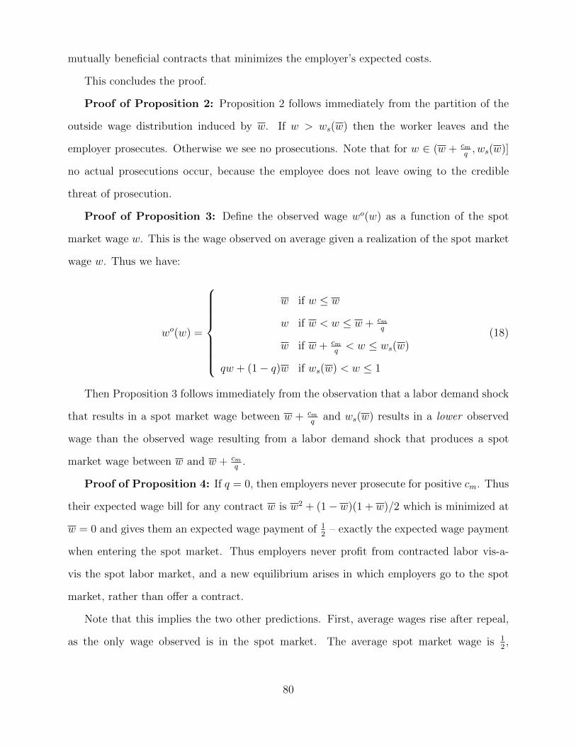
mutually beneficial contracts that minimizes the employer’s expected costs.
This concludes the proof.
Proof of Proposition 2: Proposition 2 follows immediately from the partition of the
outside wage distribution induced by w. If w > ws(w) then the worker leaves and the
employer prosecutes. Otherwise we see no prosecutions. Note that for w ∈ (w + cmq, ws(w)]
no actual prosecutions occur, because the employee does not leave owing to the credible
threat of prosecution.
Proof of Proposition 3: Define the observed wage wo(w) as a function of the spot
market wage w. This is the wage observed on average given a realization of the spot market
wage w. Thus we have:
wo(w) =
w if w ≤ w
w if w < w ≤ w + cmq
w if w + cmq< w ≤ ws(w)
qw + (1− q)w if ws(w) < w ≤ 1
(18)
Then Proposition 3 follows immediately from the observation that a labor demand shock
that results in a spot market wage between w + cmq
and ws(w) results in a lower observed
wage than the observed wage resulting from a labor demand shock that produces a spot
market wage between w and w + cmq
.
Proof of Proposition 4: If q = 0, then employers never prosecute for positive cm. Thus
their expected wage bill for any contract w is w2 + (1− w)(1 + w)/2 which is minimized at
w = 0 and gives them an expected wage payment of 12
– exactly the expected wage payment
when entering the spot market. Thus employers never profit from contracted labor vis-a-
vis the spot labor market, and a new equilibrium arises in which employers go to the spot
market, rather than offer a contract.
Note that this implies the two other predictions. First, average wages rise after repeal,
as the only wage observed is in the spot market. The average spot market wage is 12,
80

and this must be greater than the average wage when prosecutions were available (under
the assumption made that a contract was signed), because the employer’s participation
constraint implies that:
E[w|w] < E[w|w] + cm(1− ws(w)) ≤ 1
2(19)
Second, repeal increases the correlation of the observed wage and the spot market wage,
and thus the labor demand shock. Note that, trivially, the observed wage (i.e., the spot
market wage) responds 1 for 1 with respect to the spot market wage – the correlation
of observed and spot market wages is 1 if prosecution is not available to employers. The
correlation between observed and spot market wages is strictly less than 1 when prosecutions
are available (under the assumption made that a contract was signed), as for any spot market
wage less than the contractual wage, the observed wage does not change in response to the
change in the spot market wage.
This concludes the proof.
81

Appendix 4: Data
In Section 3.1, we provide a brief description of the data used in our empirical analysis. Here,
we provide a more detailed discussion of the sources of our data as well as the construction of
variables.
Prosecutions
The prosecutions of labor-market-related criminal offenses (Master and Servant, anti-vagrancy,
and anti-begging) come from Judicial Statistics, England and Wales, covering the years 1858-
1875. These are recorded for each year at the district level, in Table 7, “Offences Determined
Summarily,” under the headings “Servants, Apprentices, or Masters, Offenses relating to,”
“Having no visible Means of Subsistence, &c.,” and “Begging.” We sum district-level data
by county to generate county-level prosecutions for each year. The measure of anti-vagrancy
prosecutions used in our empirical analysis is the sum of anti-vagrancy and anti-begging
prosecutions in a district in each year.
County Characteristics
Our analysis of sector-specific labor demand shocks requires us to identify districts (in prac-
tice, counties) where iron, coal, and textile production were located in the second half of the
19th century. A continuous measure of industry presence is available for textile production:
the share of the male labor force in the “textile” category in a county in 1851 (occupational
distributions from British censuses are available on the UK data archive website, study 4559
(Southall et al., 2004). Because the census occupational categories that include coal mining
and iron production also include employment in other sectors, we use dummy variables to
indicate production of coal and of pig iron, respectively.28 Our list of coal-producing counties
comes from counties listed in Mitchell (1988), Fuel and Energy, 3 and Fuel and Energy, 5,
compared with discussion and maps in Church (1986); counties that produced pig iron are
identified from Mitchell (1988), Metals, 2.29
28Coal mining is grouped with other forms of mining, and iron production is grouped with other workrelated to metals.
29The coal producing counties are: Carmarthenshire, Cheshire, Cumberland, Denbighshire, Derbyshire,Durham, Flintshire, Glamorganshire, Gloucestershire, Lancashire, Leicestershire, Monmouthshire, Northum-
82

To address concerns about the endogeneity of the location of textile and pig iron produc-
tion, we use a county’s iron ore production in 1855 as an instrument for pig iron production
and distance to Lancashire as an instrument for the occupational share of textiles in a
county in 1851. Iron ore production data come from Minerals (1856); distance to Lancashire
is calculated as the average of every point in a county’s shortest distance to the Lancashire
border.
The county characteristics that we use as control variables in our analyses come from
several sources. Each county’s proportion urban, log income, log population, and fraction
illiterate are available for the census years online, at the UK data archive website, study 430
(Hechter, 1976).30 In our analyses, we either use 1851 values of these county characteristics,
and allow them to have year-specific effects, or we linearly interpolate values between census
years. To control for the effects of unionization on prosecutions or wages, we use data on
membership in the Amalgamated Society of Engineers (ASE), measured at the county-year
level. County-years with no branch membership listed are assigned values of zero. These
data come from the UK data archive website, study 3712 (Southall et al., 1998). We also
use the data on members of the ASE to calculate a strike rate and an unemployment rate,
which we also include in some specifications as controls. The strike rate is the fraction of
members receiving “contingent benefit” (i.e., strike pay), with the value undefined if a county
year has no ASE members. The unemployment rate is the fraction of members receiving
donation benefit (other than those members receiving contingent benefit); again, the value is
undefined if a county has no ASE members in a given year.31 Finally, we generate a recession
indicator variable using dates of business cycle peaks and troughs between 1860 and 1914,
berland, Nottinghamshire, Pembrokeshire, Somersetshire, Staffordshire, Warwickshire, Worcestershire, andYorkshire. Pig iron producing counties are: Anglesey, Brecknockshire, Cardiganshire, Carmarthen-shire, Carnarvonshire, Cumberland, Denbighshire, Derbyshire, Durham, Flintshire, Glamorganshire, Lan-cashire, Leicestershire, Lincolnshire, Merionethshire, Monmouthshire, Montgomeryshire, Northamptonshire,Northumberland, Nottinghamshire, Pembrokeshire, Radnorshire, Shropshire, Staffordshire, and Yorkshire.
30Illiteracy data for some counties are missing.31Along with the obvious concern that union members’ unemployment rates may not be representative of
workers as a whole, one is also concerned that the unemployment rate may reflect changes in the extensionof unemployment benefits by labor unions, rather than changes in unemployment.
83

taken from Ford (1981), and allow recessions to have county-specific effects in some of our
specifications.
Prices
We use three price time series to indicate sector-specific changes in labor demand. For
the coal sector, we use the log of an index of the coal price at the pithead, taken from
Church (1986), Table 1.9. To generate his index, Church uses prices received by eight to
twelve collieries (depending on the year) across Britain, for years prior to 1882 (collieries in-
clude Middleton colliery, near Leeds, Elphinstone colliery, in Scotland, and Cannock Chase
colliery in Staffordshire, among others; details are in Church’s table notes). Beginning in
1882, he uses pithead prices compiled in Mineral Statistics, an official publication.
For the iron sector, we use the log of the price (in shillings per ton) of Scottish pig
iron found in Mitchell (1988), Prices, 20.B. These prices were originally collected by Augus-
tus Sauerbeck, and published in the Journal of the Statistical Society in 1886 (“Prices of
Commodities and the Precious Metals”), then updated thereafter in the same publication.
(Cleveland pig iron prices are listed in Mitchell (1988), but only beginning in 1865; prices
of Scottish pig iron track those of Cleveland pig iron very closely throughout the period we
study.)
For cotton textiles, we use the log of the ratio of the output price of cotton textiles to
the price of raw cotton, in order to capture changes in the output price of textiles that were
not merely due to fluctuations in cotton prices. The prices of cotton textile output (in pence
per linear yard) come from Mitchell (1988), Prices, 19. The prices reported are the average
value of cotton piece goods exported in each year, not actual prices received by individual
textile producers. The original sources for these data are The Cotton Trade of Great Britain,
by T. Ellison (for prices prior to 1885) and the Annual Statement of Trade (from 1885 on).
We convert the price per linear yard of textile output into the price per pound of output
using Robson’s (1957) conversion factor of 5.47895 linear yards per pound of cotton piece
good exports (this has no effect on the analysis, but makes the interpretation of the relative
84

output price more straightforward). See Robson (1957), Table A.1, p. 333. The cotton input
prices (in pence per pound of “Upland or Middling American” cotton) come from Mitchell
(1988), Prices, 18.B. The original sources are Sessional Papers of Parliament (1903), vol. 68,
for years prior to 1903, and Augustus Sauerbeck, “Prices of Commodities and the Precious
Metals,” Journal of the Royal Statistical Society (1904, then updated), for years after 1902.
We also control for steel price shocks in our analysis of the repeal of penal sanctions. Our
steel price data are from McCloskey (1973), whose sources are Carr and Taplin’s History of
the British Steel Industry (1962) and Burn’s The Economic History of Steelmaking, 1867-
1939 (1940).
Wages
We construct a panel dataset of wages at the county-year level by combining several wage
datasets. First, we use a panel of wages at the city-year level taken from the U.K. Data
Archive, study 3710 (Southall et al., 1999). These wages were initially collected by Southall,
Gilbert, and Gregory from Rates of Wages and Hours of Labour in various industries in the
United Kingdom for a series of years, a report of the Board of Trade Labour Department.
We calculate a wage index for carpenters, painters, and bricklayers and average these to cre-
ate a single builders’ wage index at the city-year level. We then assign to each county-year
the average builders’ wage index value for the cities in that county in the relevant year.
Coal hewers’ wages at the region-year level are taken from an index found in Church
(1986), Table 7.15. The regions are the following: Scotland, the Northeast of England,
Cumberland, Lancashire and Cheshire, North Wales, Yorkshire, the East Midlands, the
West Midlands, South Wales, and the Southwest of England. We assign each coal-producing
county in our dataset to one of these regions. The original sources of these data for years
prior to 1871 are a variety of official publications and academic publications (for example,
a report by the Midland Mining Commission, and several PhD theses). Beginning in 1871,
publications from the Board of Trade provide most of the information (“Rates of Wages
and Hours of Labor in Various Industries in the United Kingdom, 1850-1905” and “Annual
85

Returns of Rates of Wages and Hours of Labor, 1893-1913”), though Church supplements this
material with other information from both official and scholarly publications (for example,
a publication by the Royal Commission on Labor).
Time series of agricultural workers’ wages, engineers’ wages, and cotton factory workers’
wages are taken from Mitchell (1988), Labour Force, Table 25. The original sources for this
table are articles published by A.L. Bowley and G.H. Wood in the Journal of the Royal
Statistical Society in 1898 and 1899, and A.L. Bowley’s Wages and Income since 1860.
We convert each wage dataset into an index with value 100 in the year 1900. Then, we
combine the several wage indices to produce a panel of wages at the county-year level, using
each county’s occupational distribution in the 1851 British census (taken from the UK data
archive website, study 4559 (Southall et al., 2004)) to weight each index in a given county-
year. Specifically, we calculate a wage at the county-year level by weighting each wage index
by men’s employment in the relevant industry, relative to men’s employment in all of the
county’s industries for which we have wage data. For example, a coal-producing county for
which builders’ wages are available would have its coal wage in a given year multiplied by
the number of men in that county in 1851 working in mining, divided by the number of
men in that county working in mining, agriculture, engineering of various sorts, textiles, and
construction in 1851.
As noted in the text, we also constructed an alternative wage panel that allowed occu-
pational shares in each county to vary over time. In this case, a coal-producing county for
which builders’ wages are available would have its coal wage in a given year multiplied by
the interpolated number of men in that county working in mining in that year, divided by
the interpolated number of men in that county working in mining, agriculture, engineering
of various sorts, textiles, and construction in that year (where the interpolations are based
on census data taken from the UK data archive website, study 4559 (Southall et al., 2004)).
Another alternative wage panel was constructed by including iron smiths’ wages from
Bowley and Wood (1906), and using the same weighting scheme as in our baseline panel.
86

As noted above, the drawback of using iron smiths’ wages is that there is no satisfactory
occupation share with which to weight the wage data: the census occupational category
that is best suited includes metal workers of all types, those who produce metal and those
who use it as an input. Next, we constructed another panel, using our baseline wage series,
but using for weights the occupation shares for all workers, not only the men’s. Finally, we
constructed another panel constructed just as in our baseline panel, but dropping the wages
of workers most likely to be white collar workers: engineers and shipbuilders.
87