cognition resubmission final - stanford universitydco/pubs/2015_affective_cognition... ·...

Lay theories of emotion 1

RUNNING HEAD: Lay theories of emotion

Affective Cognition: Exploring lay theories of emotion

Desmond C. Ong, Jamil Zaki, and Noah D. Goodman

Department of Psychology, Stanford University

Manuscript submitted to: Cognition

Revision dated: 12 June 2015

Address Correspondence to:

Desmond C. Ong Department of Psychology Stanford University Stanford, CA 94305 [email protected] Word count: Main Text: 14,654, Supplementary: 1,647, References: 2,510 Abstract word count: 215 Number of references: 115


ABSTRACT

Humans skillfully reason about others’ emotions, a phenomenon we term affective

cognition. Despite its importance, few formal, quantitative theories have described

the mechanisms supporting this phenomenon. We propose that affective cognition

involves applying domain-‐general reasoning processes to domain-‐specific content

knowledge. Observers’ knowledge about emotions is represented in rich and

coherent lay theories, which comprise consistent relationships between situations,

emotions, and behaviors. Observers utilize this knowledge in deciphering social

agents’ behavior and signals (e.g., facial expressions), in a manner similar to rational

inference in other domains. We construct a computational model of a lay theory of

emotion, drawing on tools from Bayesian statistics, and test this model across four

experiments in which observers drew inferences about others’ emotions in a simple

gambling paradigm. This work makes two main contributions. First, the model

accurately captures observers’ flexible but consistent reasoning about the ways that

events and others’ emotional responses to those events relate to each other. Second,

our work models the problem of emotional cue integration—reasoning about others’

emotion from multiple emotional cues—as rational inference via Bayes’ rule, and we

show that this model tightly tracks human observers’ empirical judgments. Our

results reveal a deep structural relationship between affective cognition and other

forms of inference, and suggest wide-‐ranging applications to basic psychological

theory and psychiatry.


Keywords: Emotion; Inference; Lay Theories; Bayesian models; Emotion Perception;

Cue Integration


1. Introduction

It is easy to predict that people generally react positively to some events (winning

the lottery) and negatively to others (losing their job). Conversely, one can infer,

upon encountering a crying friend, that it is more likely he has just experienced a

negative, not positive, event. These inferences are examples of reasoning about

another’s emotions: a vital and nearly ubiquitous human skill. This ability to reason

about emotions supports countless social behaviors, from maintaining healthy

relationships to scheming for political power. Although it is possible that some

features of emotional life carries on with minimal influence from cognition,

reasoning about others’ emotions is clearly an aspect of cognition. We propose

terming this phenomenon affective cognition—the collection of cognitive processes

that involve reasoning about emotion.

For decades, scientists have examined how people manage to make complex

and accurate attributions about others’ psychological states (e.g., Gilbert, 1998;

Tomasello, Carpenter, Call, Behne, & Moll, 2005; Zaki & Ochsner, 2011). Much of this

work converges on the idea that individuals have lay theories about how others

react to the world around them (Flavell, 1999; Gopnik & Wellman, 1992; Heider,

1958; Leslie, Friedman, & German, 2004; Pinker, 1999). Lay theories—sometimes

called intuitive theories or folk theories—comprise structured knowledge about the

world (Gopnik & Meltzoff, 1997; Murphy & Medin, 1985; Wellman & Gelman, 1992).

They provide an abstract framework for reasoning, and enable both explanations of

past occurrences and predictions of future events. In that sense, lay theories are

similar to scientific theories—both types of theories are coherent descriptions of


how the world works. Just as a scientist uses a scientific theory to describe the

world, a lay observer uses a lay theory to make sense of the world. For instance,

people often conclude that if Sally was in another room and did not see Andy switch

her ball from the basket to the box, then Sally would return to the room thinking

that her ball was still in the basket: Sally holds a false belief, where her beliefs about

the situation differs from reality (Baron-‐Cohen, Leslie, & Frith, 1985). In existing

models, this understanding of others’ internal states is understood as a theory that

can be used flexibly and consistently to reason about other minds. In this paper, we

propose a model of how people likewise reason about others’ emotions using

structured lay theories that allow complex inferences.

Within the realm of social cognition, lay theories comprise knowledge about

how people’s behavior and mental states relate to each other, and allow observers

to reason about invisible but important factors such as others’ personalities and

traits (Chiu, Hong, & Dweck, 1997; Heider, 1958; Jones & Nisbett, 1971; Ross, 1977;

Ross & Nisbett, 1991), beliefs and attitudes (Kelley & Michela, 1980), and intentions

(Kelley, 1973; Jones & Davis, 1965; Malle & Knobe, 1997). Crucially, lay theories

allow social inference to be described by more general principles of reasoning. For

example, Kelley (1973)’s Covariational Principle describes how observers use

statistical co-‐variations in observed behavior to determine whether a person’s

behavior reflects a feature of that person (e.g., their preferences or personality) or a

feature of the situation in which they find themselves. There are many similar

instances of lay-‐theory based social cognition: Figure 1 lists just several such

examples, such as how lay theories of personality (e.g., Chiu et al, 1997), race (e.g.,


Jayaratne et al., 2006), and “theories of mind” (e.g., Gopnik & Wellman, 1992) inform

judgments and inferences—not necessarily made consciously—about traits and

mental states. Although lay theories in different domains contain vastly different

domain-‐specific content knowledge, the same common principles of reasoning—for

example, statistical co-‐variation, deduction, and induction—are domain-‐general, and

can be applied to these lay theories to enable social cognitive capabilities such as

inferences about traits or mental states.

Lay theories can be formalized using Bayesian statistics using ideal observer

models (Geisler, 2003). This approach has been used successfully to model a wide

range of phenomena in vision, memory, decision-‐making (Geisler, 1989; Liu, Knill, &

Kersten, 1995; Shiffrin & Steyvers, 1997; Weiss, Simoncelli, & Adelson, 2002), and,

more recently, social cognition (e.g., Baker, Saxe, & Tenenbaum, 2009). An ideal

observer analysis describes the optimal conclusions an observer would make given

(i) the observed evidence and (ii) the observer’s assumptions about the world. Ideal

observer models describe reasoning without making claims as to the mechanism or

process by which human observers draw these conclusions (cf. Marr, 1982), and

provide precise, quantitative hypotheses through which to explore human cognition.


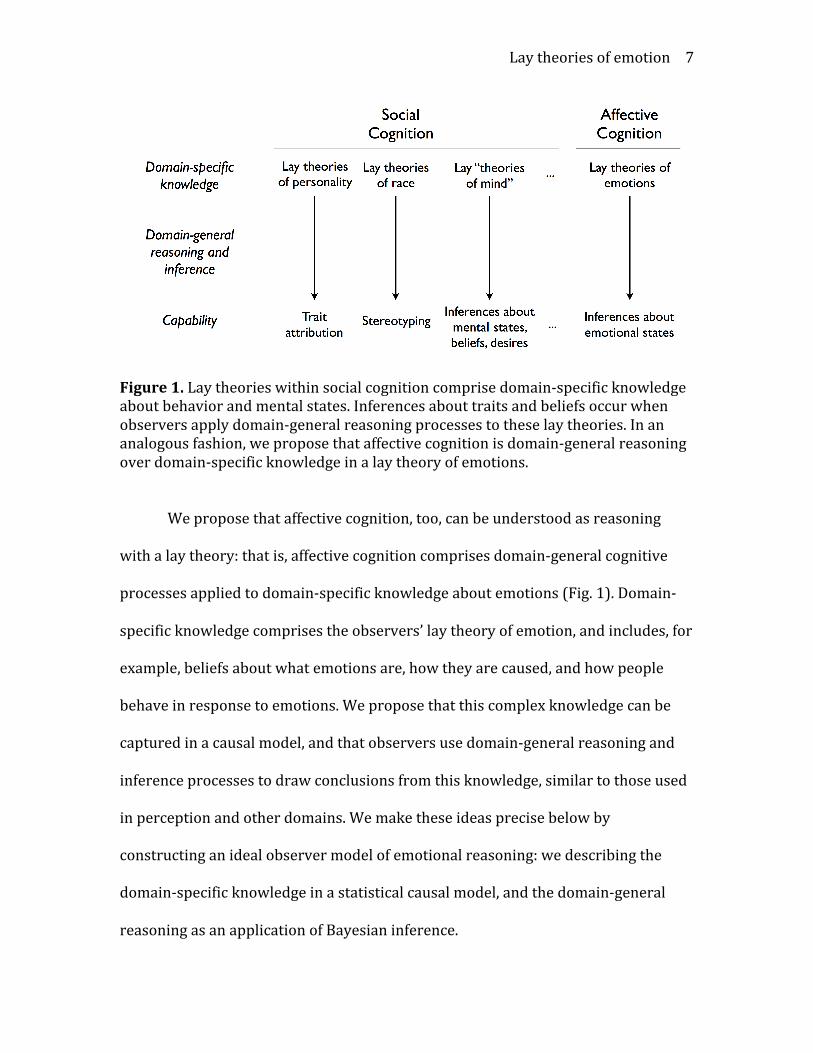
Figure 1. Lay theories within social cognition comprise domain-‐specific knowledge about behavior and mental states. Inferences about traits and beliefs occur when observers apply domain-‐general reasoning processes to these lay theories. In an analogous fashion, we propose that affective cognition is domain-‐general reasoning over domain-‐specific knowledge in a lay theory of emotions.

We propose that affective cognition, too, can be understood as reasoning

with a lay theory: that is, affective cognition comprises domain-‐general cognitive

processes applied to domain-‐specific knowledge about emotions (Fig. 1). Domain-‐

specific knowledge comprises the observers’ lay theory of emotion, and includes, for

example, beliefs about what emotions are, how they are caused, and how people

behave in response to emotions. We propose that this complex knowledge can be

captured in a causal model, and that observers use domain-‐general reasoning and

inference processes to draw conclusions from this knowledge, similar to those used

in perception and other domains. We make these ideas precise below by

constructing an ideal observer model of emotional reasoning: we describing the

domain-‐specific knowledge in a statistical causal model, and the domain-‐general

reasoning as an application of Bayesian inference.


1.1 Attributing emotional reactions

How does an observer infer that agents (the targets of affective cognition)

who spill a cup of coffee, miss the bus, or fall off a bicycle, likely feel similar

(negative) emotions? One problem that any model of affective cognition must deal

with is the combinatorial explosion of outcomes and emotional states that people

can experience. It would be both inefficient and impractical for observers to store or

retrieve knowledge about the likely affective consequences of every possible

situation. We hypothesize that people circumvent this complexity by evaluating

situations based on a smaller number of “active psychological ingredients” those

situations contain. For instance, many emotion-‐inducing situations share key

common features (e.g., the attainment or nonattainment of goals) that consistently

produce particular emotions (Barrett, Mesquita, Ochsner, & Gross, 2007; Ellsworth

& Scherer, 2003). An individual in a situation can take advantage of this

commonality by appraising the situation along a small number of relevant appraisal

dimensions: that is, reducing a situation to a low-‐dimensional set of emotion-‐

relevant features (Ortony, Clore, & Collins, 1988; Schachter & Singer, 1962; Scherer,

Schorr, & Johnstone, 2001; Smith & Ellsworth, 1985; Smith & Lazarus, 1993).

We propose that observers similarly reduce others’ experience to a small

number of emotionally relevant features when engaging in affective cognition. The

examples above—spilling coffee, missing the bus, and falling off a bicycle—could all

be associated, for instance, with unexpectedly losing something (e.g. coffee, time,

and health). Note that the features relevant to the person’s actual emotions


(identified by appraisal theories) may not be identical to the features used by the

observer (which are part of the observer’s lay theory). The latter is our focus when

studying affective cognition. Thus, we will first elucidate the situation features

relevant for attributing emotion to another person. We operationalize this in

Experiment 1 by studying a simple family of scenarios—a gambling game—and

considering a variety of features such as amount of money won, prediction error

(the amount won relative to the expected value of the wheel), and distance from a

better or worse outcome.

1.2 Reasoning from emotional reactions

A lay theory should support multiple inferences that are coherently related

to each other: we can reason from a cause to its effects, but also back from an effect

to its cause, and so on. For example, we can intuit that missing one’s bus makes one

feel sad, and we can also reason, with some uncertainty, that the frowning person

waiting forlornly at a bus stop might have just missed their bus. If affective cognition

derives from a lay theory, then it should allow observers to both infer unseen

emotions based on events, and also to infer the type of event that a social target has

experienced based on that person’s emotions. In the framework of statistical causal

models, these two types of inference—from emotions to outcomes and from

outcomes to emotions—should be related using the rules of probability. In

Experiment 2, we explicitly test this proposal: do people reason flexibly back and

forth between emotions and the outcomes that cause them? Do forward and reverse

inferences cohere as predicted by Bayesian inference?


1.3 Integrating Sources of Emotional Evidence

Domain-‐general reasoning should also explain more complex affective cognition.

For instance, observers often encounter multiple cues about a person’s emotions:

They might witness another person’s situation, but also the expression on the

person’s face, their body posture, or what they said. Sometimes these cues even

conflict—for instance, when an Olympic athlete cries after winning the gold medal.

This seems to be a pair of cues that individually suggest conflicting valence. A

comprehensive theory of affective cognition should address how observers

translate this deluge of different information types into an inference, a process we

call emotional cue integration (Zaki, 2013).

Prior work suggests two very different approaches that observers might take

to emotional cue integration. On the one hand, the facial dominance hypothesis

holds that facial expressions universally broadcast information about emotion to

external observers (Darwin, 1872; Ekman, Friesen, & Ellsworth, 1982; Smith,

Cottrell, Gosselin, & Schyns, 2005; Tomkins, 1962; for more extensive reviews, see

Matsumoto, Keltner, Shiota, O’Sullivan, & Frank, 2008; Russell, Bachorowski, &

Fernández-‐Dols, 2003). This suggests that observers should draw primarily on facial

cues in determining social agents’ emotions (Buck, 1994; Nakamura, Buck, & Kenny,

1990; Wallbott, 1988; Watson, 1972). On the other hand, contextual cues often

appear to drive affective cognition even when paired with facial expressions. For

instance, observers often rely on written descriptions of a situation (Carroll &

Russell, 1996; Goodenough & Tinker, 1931) body postures (Aviezer et al., 2008;


Aviezer, Trope, & Todorov, 2012; Mondloch, 2012; Mondloch, Horner, & Mian, 2013;

Van den Stock, Righart, & de Gelder, 2007), background scenery (Barrett &

Kensinger, 2010; Barrett, Mesquita, & Gendron, 2011; Lindquist, Barrett, Bliss-‐

Moreau, & Russell, 2006), and cultural norms (Masuda et al, 2008) when deciding

how agents feel.

Of course, both facial expressions and contextual cues influence affective

cognition. It is also clear that neither type of cue ubiquitously “wins out,” or

dominates inferences about others’ emotions. An affective cognition approach

suggests that observers should solve emotional cue integration using domain-‐

general inference processes. There are many other settings—such as binocular

vision (Knill, 2007) and multisensory perception (Alais & Burr, 2004; Shams,

Kamitani, & Shimojo, 2000; Welch & Warren, 1980)—that require people to

combine multiple cues into coherent representations. These ideal observer models

assume that observers combine cues in an optimal manner given their prior

knowledge and uncertainty. In such models, sensory cue integration is modeled as

Bayesian inference (for recent reviews, see Ernst & Bulthoff, 2004; de Gelder &

Bertelson, 2003; Kersten, Mamassian, & Yuille, 2004).

Our framework yields an approach to emotional cue integration that is

analogous to cue integration in object perception: a rational information integration

process. Observers weigh available cues to an agent’s emotion (e.g., the agent’s facial

expression, or the context the agent is in) and combine them using statistical

principles of Bayesian inference. This prediction naturally falls out of our claim that

affective cognition resembles other types of theory-‐driven inference, with domain-‐


specific content knowledge: the lay theory of emotion describes the statistical and

causal relations between emotion and each cue; joint reasoning over this structure

is described by domain-‐general inference processes.

We empirically test the predictions of this approach in Experiments 3 and 4.

We aim to both extend the scope of our lay theory model and resolve the current

debate in emotion perception by predicting how different cues are weighted as

observers make inferences about emotion.

1.4 Overview

We first describe the components of our model and how it can be used to

compute inferences about others’ emotions. We formalize this model in the

language of Bayesian modeling (Goodman & Tenenbaum, 2014; Goodman, Ullman, &

Tenenbaum, 2011; Griffiths, Kemp, & Tenenbaum, 2008). Specifically, we focus on

the ways that observers draw inferences about agents’ emotions based on the

situations and outcomes those agents experience. In all our experiments, we

restricted the types of situations that agents experience to a simple gambling game.

Although this paradigm does not capture many nuances of everyday affective

cognition, its simplicity allowed us to quantitatively manipulate features of the

situation and isolate situational features that best track affective cognition.

Experiment 1 sheds light on the process of inferring an agent’s emotions

given a situation, identifying a set of emotion-‐relevant situation features that

observers rely on to understand others’ affect. Experiment 2 tests the flexibility of

emotional lay theories, by testing whether they also track observers’ reasoning


about the outcomes that agents’ likely encountered based on their emotions; our

model’s predictions tightly track human judgments.

We then expand the set of observable evidence that our model considers, and

describe how our model computes inferences from multiple cues—emotional cue

integration. Experiment 3 tests the model against human judgments of emotions

from both situation outcomes and facial expressions; Experiment 4 replicates this

with situation outcomes and verbal utterances. In particular, we show that the

Bayesian model predicts human judgments accurately, outperforming the baseline

single cue dominance (e.g. facial or context dominance) models. Together, the

results support the claim that reasoning about emotion represents a coherent set of

inferences over a lay theory, similar to reasoning in other domains of psychology.

Finally, we describe some limitations of our model, motivate future work,

and discuss the implications of an affective cognition approach for emotion theory,

lay theories in other domains, and real-‐world applications.

2. Exploring the flexible reasoning between outcomes and emotions

Our model of a lay theory of emotion is shown schematically in Figure 2. An

observer (i.e. the reasoner) uses this lay theory to reason about an agent (i.e. the

target of the reasoning). There are emotion-‐eliciting situations in the world, and the

outcomes of these situations, interacting with other mental states such as goals,

cause an agent to feel emotions. The agent’s emotions in turn produce external

cues including facial expressions, body language, and speech, as well as further


actions. All of these variables, except mental states such as emotion and goals, are

potentially observable variables; in particular, emotion is a latent variable that is

unobservable because it is an internal state of the agent.

Figure 2. Model of a lay theory that an observer could use during affective cognition. Using the notation of Bayesian networks, we represent variables as circles, and causal relations from a causal variable to its effect as arrows. Shaded variables represent unobservable variables. Although causal flows are unidirectional, as indicated by the arrows, information can flow the other way, as when making inferences about upstream causes from downstream outcomes. In this model, observers believe that situation outcomes cause an agent to feel an emotion, which then causes certain behavior such as speech, facial expressions, body language or posture, and importantly, actions that potentially result in new outcomes and a new emotion cycle. From the observable variables—which we call “cues”—we can infer the agent’s latent, or unobservable, emotion. Other mental states could be added to this model. One such extension includes the agent’s motivational states or goals, which would interact with the outcome of a situation to produce emotions; such goals would also influence the actions taken.

Each of these directed causal relationships can be represented as a

probability distribution. For example, we can write different levels of happiness and

anger given the outcome of winning the lottery as P(happy | won lottery) and

P(angry | won lottery). In our model, we represent the relationship between general


outcomes o and emotions e as P(e|o). Similarly, the causal relationship between an

agent’s emotions and his resultant facial expressions f can be written as P(f|e), and

so forth.

As we discussed above, it would be impractical for observers to store the

affective consequences of every possible situation outcome (i.e., P(e|o) for every

possible outcome o). We hypothesize that observers reduce the multitude of

possible outcomes into a low-‐dimensional set of emotion-‐relevant features via, for

example, appraisal processes (e.g., Ortony et al., 1988). One potentially important

outcome feature is value with respect to the agent’s goals. Indeed, a key

characteristic of emotion concepts, as compared to non-‐emotion concepts, is their

inherent relation to a psychological value system (Osgood, Suci, & Tannenbaum,

1957), that is, representations of events’ positive or negative affective valence

(Clore et al, 2001; Frijda, 1998). As economists and psychologists have long known,

people assess the value of events relative to their expectations: winning $100 is

exciting to the person who expected $50 but disappointing to the person who

expected $200 (Carver & Scheier, 2004; Kahneman & Tversky, 1979). Deviations

from an individual’s expectation are commonly termed prediction errors, and

prediction errors in turn are robustly associated with the experience of positive and

negative affect (e.g., Knutson, Taylor, Kaufman, Peterson, & Glover, 2005).

Responses to prediction errors are not all equal, however; individuals tend to

respond more strongly to negative prediction errors, as compared to positive

prediction errors of equal magnitude, a property commonly referred to as loss

aversion (Kahneman & Tversky, 1984). These value computations are basic and


intuitively seem linked to emotion concepts, and we propose that they form an

integral part of observers’ lay theory of emotion. Thus, we hypothesize that reward,

prediction error, and loss aversion constitute key outcome features that observers

will use to theorize about others’ emotions, and facilitate affective cognition. Other,

less “rational” features likely also influence affective cognition. Here we consider

one such factor: the distance from a better (or worse) outcome, or how close one

came to achieving a better outcome. In Experiment 1 we explore the situation

features that parameterize P(e|o) in a simple gambling scenario.

Although the lay theory we posit is composed of directed causal

relationships—signaled by arrows in Figure 2—people can also draw “reverse

inferences” about causes based on the effects they observe (for instance, a wet front

lawn offers evidence for the inference that it has previously rained.). In addition to

reasoning about emotions e given outcomes o, observers can also draw inferences

about the posterior probability of different outcomes o having occurred, given the

emotion e. This posterior probability is written as P(o|e) and is specified by Bayes’

Rule:

P o | e( ) =P e | o( )P o( )

P(e)

(1)

where P(e) and P(o) represent the prior probabilities of emotion e and outcome o

occurring, respectively. By way of example, imagine that you walk into your friend’s

room and find her crying uncontrollably; you want to find the outcome that made

her sad—likely the o with the highest P(o|sad)—so you start considering possible

candidate outcomes using your knowledge of your friend. She is a conscientious and


hardworking student, and so if she fails a class exam, she would be sad, i.e.,

P(sad|fail exam) is high. But, you also recall that she is no longer taking classes, and

so the prior probability of failing an exam is small, i.e., P(fail exam) is low. By

combining those two pieces of information, you can infer that your friend probably

did not fail an exam, i.e., P(fail exam|sad) is low, and so you can move on and

consider other possible outcomes. In Experiment 2 we consider whether people’s

judgments from emotions to outcomes are predicted by the model of P(e|o)

identified in Experiment 1 together with Bayes’ rule.

2.1 Experiment 1: Emotion from Outcomes1

Our first goal is to understand how P(e|o) relates to the features of a situation and

outcome. We explore this in a simple gambling domain (Fig. 3) where we can

parametrically vary a variety of outcome features, allowing us to understand the

quantitative relationship between potential features and attributed emotions.

2.1.1 Participants. We recruited one hundred participants through

Amazon’s Mechanical Turk and paid them for completing the experiment. All

experiments reported in this paper were conducted according to guidelines

approved by the Institutional Review Board at Stanford University.

2.1.2 Procedures. Participants played the role of observers and watched

characters play a simple gambling game. These characters each spun a wheel and

won an amount of money depending on where the wheel landed (Fig. 3). On each

trial, one character spun one wheel. We pre-‐generated a total of 18 wheels. Each 1 Materials, data, and code can be found at: github.com/desmond-‐ong/affCog


wheel comprised three possible outcomes, all of which were non-‐negative. We

systematically de-‐correlated the probabilities of the outcomes and the values of the

outcomes of each wheel, allowing for separate calculation of reward amount and

expected value. We used a standard definition of expected value: the averaged

reward that the character expected to win. For each “wedge”, or sector of the wheel,

we take the reward amount on that sector, and multiply it with the notational

probability—based on the size—of that sector. The expected value is the sum of

these products over all the sectors. The final correlation of the amount won with the

expected value was 0.3. The 18 wheels with 3 outcomes each resulted in (after

discarding one to make a number that could be evenly divided by total trials) 50

scenarios, where each scenario corresponds to a particular outcome on a particular

wheel. On each trial, the experimental program selected the scenario (the particular

outcome to be won) randomly from the total set of 50 scenarios, and not

proportional to the sector size within a wheel2. This was a design choice to ensure

that small sectors (with low notational probability) were equally represented in the

data. This fact was not obvious to the participants, and we assume that participants

treated the wheel as being fairly spun. The exact position within the sector where

the spinner lands—for example, whether the spinner lands in the center of the

sector, or near the edge of the sector, as in the example shown in Figure 3—was a

real number in the interval (0, 1) drawn from a uniform distribution.

2 The alternative, which we did not do, would be to randomly choose a wheel with all its possible outcomes from a set of all possible wheels, and then uniformly choose where it lands; each sector would then be sampled proportional to its notational probability.


Each participant completed 10 trials. On each trial, they saw a stick figure

character with a randomized male name (e.g. “Bob”) spin a wheel. The names of the

characters were randomized on every trial. After the result of the spin, participants

had to rate how the character feels, on a set of 9 point Likert scales. There were

eight different Likert scales for each of eight emotion adjectives: happy, sad, angry,

surprised, fearful, disgusted, content, and disappointed. The first six were the classic

“basic emotions” described by Ekman and colleagues (e.g., Ekman, Friesen, &

Ellsworth, 1982). We added “content” and “disappointed” to capture emotion

concepts related to counterfactual comparisons with outcomes that could have, but

did not occur (Gilovich & Medvec, 1995; Sweeney & Vohs, 2012).


Figure 3. Sample screenshots from Experiment 1. Participants see a character spin a wheel that lands, in this case, on $60. Participants then attribute emotions to the character on eight separate Likert scales.

2.1.3 Forward regression model. We expected that affective cognition

should depend on specific situation features—especially those related to value

computation—that often predict an agent’s emotions. As such, we chose several a

priori features based on previous work in decision theory as model regressors to

predict observers’ affective judgments. It is worth reiterating here that our

prediction is not that these features actually affect the ways that agents feel; that

point has been made by decades of economic and psychological research. Rather,


our prediction here is that observers spontaneously rely on these features when

inferring how others feel—in essence applying sophisticated lay theories to affective

cognition.

We predicted that reward, prediction error, and loss aversion form key

features of affective cognition. We operationalized these as regressors representing

the amount won by the agent in a trial (“win”), the prediction error (“PE”; the

difference between what the agent won and the expected value of the wheel), and

the absolute value of the prediction error (“|PE|”), respectively. Using both PE and

|PE| in the same model allows the coefficient on PE to differ when PE is positive and

negative, modeling loss aversion.3

We additionally evaluated several other a priori plausible regressors (none of

which survived model selection below). People compare their results with salient

possible counterfactuals (e.g. what they “could have” won; Medvec, Madley, &

Gilovich, 1995). To examine whether observers weigh such comparisons during

affective cognition, we computed—for each gamble—a score representing regret

(the difference between how much the agent won and the maximum he could have

won4; Loomes & Sugden, 1982) and relief (the difference between how much the

agent won and the minimum he could have won). Finally, we drew on previous work

3 Note that researchers model loss aversion as the difference between the coefficient of PE when PE is negative and when PE is positive, often using a piecewise function. It is often modeled using the piecewise equations: y=a PE, for PE>0, and y=b PE, for PE<0. We chose to adopt a mathematically equivalent formulation using both PE and |PE| as regressors in the same model: y=c PE + d |PE| across all values of PE. We can easily show that a = c + d, and b = c – d. 4 Note that this ‘game-‐theoretic’ definition of regret (over outcomes given a specified choice) is slightly distinct from most psychological definitions that involve regret over choices. We chose not to call this variable disappointment (usually contrasted with regret), as that was one of the emotions we measured.


on “luck” (e.g. Teigen, 1996), where observers tend to attribute more “luck” to an

agent who won when the chances of winning were low, even after controlling for

expected payoffs. To model whether observers account for this when attributing

other emotions, we included a regressor to account for the probability of winning,

i.e., the size of the sector that the wheel landed on. Since a probability is bounded in

[0,1] and the other regressors took on much larger domains of values (e.g. win

varied from 0 to 100), we used a logarithm to transform the probability to make the

values comparable to other regressors (“logWinProb”).

The final regressor we included was a “near-‐miss” term to model agents’

affective reactions to outcomes as a function of their distance from other outcomes.

Such counterfactual reasoning often affects emotion inference. For instance, people

reliably judge someone to feel worse after missing a flight by 5 minutes, as

compared to 30 minutes (Kahneman & Tversky, 1982). Near-‐misses “hurt” more

when the actual outcome is close (e.g., in time) to an alternative, better outcome. In

our paradigm, since outcomes are determined by how much the wheel spins,

“closeness” can be operationalized in terms of the angular distance between (i)

where the wheel landed (the actual outcome; as defined by the pointer) and (ii) the

boundary between the actual outcome and the closest sector. We defined a

normalized distance, which ranged from 0 to 0.5, with 0 being at the boundary edge,

and 0.5 indicating the exact center of the current sector. Near-‐misses have much

greater impact at smaller distances, so we took a reciprocal transform5 (1/x) to

5 We tried other non-‐linear transforms such as exponential and log transforms, which all performed comparably.


introduce a non-‐linearity that favors smaller distances. Finally, we scaled this term

by the difference in payment amounts from the current sector to the next-‐nearest

sector, to weigh the near-‐miss distance by the difference in utility in the two payoffs.

In total, we tested seven outcome variables: win, PE, |PE|, regret, relief,

logWinProb and nearMiss. We fit mixed-‐models predicting each emotion using these

regressors as fixed effects, and added a random intercept by subject. We performed

model selection by conducting backward stepwise regressions to choose the optimal

subset of regressors that predicted a majority of observers’ ratings of the agents’

emotions. This was done using the step function in the R package lmerTest.

Subsequently, we used the optimal subset of regressors as fixed effects with the

same random effect structure. Full details of the model selection and results are

given in Appendix A.

2.1.4 Results. Model selection (in Appendix A) revealed that participants’

emotion ratings were significantly predicted only by three of the seven regressors

we initially proposed: amount won, the prediction error (PE), and the absolute value

of the prediction error (|PE|) (see also Section 3.3 for a re-‐analysis with more data).

Crucially, PE and |PE| account for significant variance in emotion ratings after

accounting for amount won. This suggests that affective cognition is remarkably

consistent with economic and psychological models of subjective utility. In

particular, emotion inferences exhibited reference-‐dependence—tracking prediction

error in addition to amount won—and loss aversion—in that emotion inferences

were more strongly predicted by negative, as opposed to positive prediction error.

These features suggest that lay observers spontaneously use key features of


prospect theory (Kahneman & Tversky, 1979, 1984) in reasoning about others’

emotions: a remarkable connection between formal and everyday theorizing. It is

worth noting as well that the significant regressors for surprise followed a slightly

different pattern from the rest of the other emotions, where the win probability, as

well as regret and relief, seem just as important as the amount won, PE, and |PE|.

The aforementioned analysis suggests that amount won, PE, and |PE| are

necessary to model emotion inferences in a gambling context and suggest a low

dimensional structure for the situation features. Next, we explored the underlying

dimensionality of participants’ inferences about agents’ emotions via an a priori

planned Principal Component Analysis (PCA). Previous work on judgments of facial

and verbal emotions (e.g., Russell, 1980; Schlosberg, 1954) and self-‐reported

emotions (e.g., Kuppens et al., 2012; Watson & Tellegen, 1985) have suggested a

low-‐dimensional structure, and we planned this analysis to see if a similar low-‐

dimensional structure might emerge in attributed emotions in our paradigm.

The first principal component (PC) accounted for 59% of the variance in

participants’ ratings along all 8 emotions, while the second PC accounted for 16%;

subsequent PCs individually explained less than 10% of the variance. The first PC

accounted for most of the variance in the emotion ratings, although the second PC

accounted for a far lower, but still noteworthy, amount of variance. Full details of

the PCA procedure and loading results are given in Appendix A.

Post-‐hoc exploratory analysis of the first two PCs revealed that the first PC

positively tracked happiness and contentment, while negatively tracking all negative

emotions; by contrast, the second PC positively tracked the intensity of both positive


and negative emotions (Fig. 4A). Interestingly, this connects with classic concepts of

valence and arousal, respectively, which feature centrally in emotion science6 (e.g.,

Russell, 1980; Schlosberg, 1954, Kuppens et al., 2012). In particular, some theorists

view emotional valence as a crucial form of feedback to the agent: positively

valenced emotions like happiness signal a positive prediction error—that the agent

is doing better than expected—hence, positively reinforcing successful behavior.

Conversely, negatively valenced emotions could signal to the agent to change some

behavior to achieve a better outcome (e.g., Carver & Scheier, 2004; Ortony, Clore, &

Collins, 1988). In line with this, we find that the first PC (“valence”) of emotions

attributed by the observer correlated strongly with the PE of the situation (r =

0.737, 95% C.I. = [0.707; 0.764]). Additionally, we find that the second PC

(“arousal”) correlated with |PE| (r = 0.280 [0.222, 0.364]; Fig. 4B).

6 We invite the reader to compare the striking similarity between our Figure 4A with similar valence-‐arousal figures in the literature, such as Figure 1 from Russell (1980) and Figure 2A from Kuppens et al., (2012).


Figure 4. (A) Participants’ emotion ratings projected onto the dimensions of the first two principal components (PCs), along with the loadings of the PCs on each of the eight emotions. The loading of the PCs onto the eight emotions suggests a natural interpretation of the first two PCs as “valence” and “arousal” respectively. The labels for disgust and anger are overlapping. (B) Participant’s emotion ratings projected onto the dimensions of the first two PCs, this time colored by the prediction error (PE = amount won – expected value of wheel).

We started with a priori predictions for a low-‐dimensional summary of

outcome features, and followed up with a post-‐hoc dimensionality reduction

analysis of the emotion ratings. It is intriguing that the low-‐dimensional value

computations (e.g. PE, |PE|) are intimately tied with the principal components of the

emotion ratings (“valence” and “arousal”). However, note that the second PC

(“arousal”) accounts for much less variance than the first PC (“valence”). One

possibility is that the paradigm we used is limited in the range of emotions that it

elicits in an agent, which restricts the complexity of emotion inferences in this

paradigm. A second possibility is that emotional valence is the central feature of

affective cognition, and valence would carry most of the variance in emotion


inferences across more complex scenarios. Although we are not able to address the

second possibility in this paper, there is much theoretical evidence from affective

science (e.g., Barrett & Russell, 1999; Russell, 1980; Schlosberg, 1954) in favor of the

second possibility; future work is needed to explore this further.

Together, these findings provide two key insights into the structure of

affective cognition: (i) lay theories of emotion are low dimensional, consistent with

affective science concepts of valence and arousal, and (ii) these core dimensions of

emotion inference also track aspects of the situation and outcome that reflect value

computation parameters described by economic models such as prospect theory.

Although the specific structure of affective cognition likely varies depending on the

complexity and details of a given context, we believe that observers’ use of low-‐

dimensional “active psychological ingredients” in drawing inferences constitutes a

core feature of affective cognition.

2.2 Experiment 2: Outcomes from Emotions

Experiment 1 established the features that allow observers to reason about

agents’ emotions given a gamble outcome: representing P(e|o) in a simple linear

model. In Experiment 2 (Fig. 5), we test the hypothesis that participants’ lay

theories are flexible enough to also allow “backward” inferences about the situation

outcome based on emotions. These backward inferences are predicted from the

forward regression model by Bayes’ rule. To evaluate our model’s predictions, we

show participants the emotions of characters who have played the same game

show—importantly, without showing the eventual outcome—and elicit participants’


judgments about the likely outcome. We then compare the empirical judgments (in

Experiment 2) to the posterior probabilities predicted by the model (based on data

from Experiment 1).

2.2.1 Participants. We recruited one hundred twenty-‐five participants via

Amazon Mechanical Turk. We excluded three participants because they reported

technical difficulties with the animation, resulting in a final sample size of 122.

2.2.2 Stimuli. We generated graphical emotion profiles that ostensibly

represented the emotions that the agent feels after each outcome (Fig. 5B). These

emotion profiles were shown on continuous slider scales that corresponded to each

individual emotion. For each of the outcomes, we used the average emotion ratings

given by participants in Experiment 1 to generate the emotion profiles seen by

participants in Experiment 2. Specifically, for each outcome, we drew eight emotion

values from Gaussians with means and standard deviations equal to the means and

standard deviations of the emotion ratings given by participants in response to that

outcome in Experiment 1. This was meant to provide naturalistic emotion profiles

for the participants in Experiment 2.

2.2.3 Procedures. Each participant completed 10 trials, randomly drawn

from the same 50 pre-‐generated scenarios used in Experiment 1. On each trial,

participants were shown a stick figure and the game wheel, as before. This time, as

the wheel spun, a gray square covered the wheel, occluding the outcome (Fig. 5A).

Participants were then shown a graphical representation of the agent’s emotions

after seeing the outcome (Fig. 5B). For instance, on a particular trial, a participant

might see three possible gamble outcomes of $25, $60, and $100. Without being able


to see where the wheel landed, they might then be told that the agent who spun the

wheel, following its outcome, feels moderately happy (e.g., a slider at about a 6 on a

9 point scale), not at all sad (e.g., another slider that shows between a 1 and 2 on a 9

point scale), and so forth; see Figure 5 for an illustration. Participants were then

asked to infer how likely it was that each of the three possible outcomes had

occurred. They gave probability judgments on 9 point Likert scales. Hence, on each

trial, they gave three likelihood judgments, which corresponded to each of the three

possible outcomes.

Progress bar: 0/10

Chris is going to spin this wheel.

He will win the amount of money shown in the section the wheel lands on (indicated by the black pointer). Please

study the wheel closely: make sure you know how much he would win for each section, and how large each section

is.

After the wheel is spun, the result will be hidden from you but not from Chris.

(The wheel will spin for a few more seconds after it is hidden. There might be a slight graphical artefact on some

browsers as the wheel is covered, please ignore it.)

Click on the ``Go"ʺ button when you are ready.

After seeing the outcome, this is how much Chris feels each of the following emotions:

How much do you think Chris has won?

How likely is it that the wheel landed on the outcome $25? e.g. : Not at all likely Extremely Likely

$25

$60

$100

Go!(The wheel before it was spun)

$25

$60 $100

Less More

Happy

Sad

Angry

Surprised

Disgusted

Fearful

Content

Disappointed

$25

$60

$100

Happy

Sad

Angry

Surprised

Disgusted

Fearful

Content

Disappointed

B

A


Figure 5. Screenshots from Experiment 2. (A) Participants were shown a character that spins a wheel, but a grey square then occludes the outcome on the wheel. (B) Participants then saw a graphical representation of the character’s emotions, and inferred separate probabilities for each of the three possible outcomes having occurred.

2.2.4 Bayesian model details. In order to generate model-‐based predictions

about observers’ “reverse inference” about outcomes given emotions, the posterior

P(o|e), one needs three components: P(o), P(e), and P(e|o) (Eqn. 1). The prior

probabilities of the outcomes P(o) here are given by the notational probability of

each outcome on the wheel—i.e. the relative size of each outcome—and are

transparent to an observer in our paradigm. Larger sectors have higher

probabilities of that outcome occurring. One actually does not need to explicitly

calculate the prior probability of the emotion P(e) as long as we properly normalize

P(o|e).7

The crucial step lies in calculating the likelihood P(e|o). To calculate P(e|o),

we drew on the “forward reasoning” data collected in Experiment 1. In particular,

we leveraged Experiment 1’s regression model to calculate the extent to which

observers would be likely to infer different emotions of an agent based on each

outcome. To do so, we applied the variables identified as most relevant to affective

cognition in Experiment 1—win, PE, and |PE|—to predict the emotions observers

would assign to agents given the novel outcomes of Experiment 2. For instance, in

7 Consider calculating the posteriors of the three possible outcomes given an observed value of happiness, h : P(o1|h), P(o2|h), and P(o3|h), which are proportional to [P(h|o1)P(o1)], [P(h|o2)P(o2)], and [P(h|o3)P(o3)] respectively. The sum of the latter three quantities is simply the prior on emotion P(h). Thus, as long as proper normalization of the probabilities is carried out (i.e. ensuring that the posteriors all sum to 1), we do not need to explicitly calculate P(h) in our calculation of P(o|h). This is true for the other emotions in the model.


modeling happiness, this approach produces the following equation for each wheel

outcome:

happy = c0,happy + c1,happywin+ c2,happyPE + c3,happy | PE |+εhappy

(2)

We employed similar regression equations to estimate P(e|o) for the other seven

emotions, where εemotion (with zero mean and standard deviation σ emotion ) represents

the residual error terms of the regressions. The coefficients ci,emotion are obtained

numerically by fitting the data from Experiment 1; the linear model is fit across all

participants and scenarios to obtain one set of coefficients per emotion. For a new

scenario with {win, PE, |PE|}, the likelihood of observing a certain happy value h ' is

simply the probability that h ' is drawn from the linear model. In other words, it is

the probability that the error

(3)

is drawn from the residual error distribution for εhappy .

The error distribution resulting from the above regression captures

intrinsic noise in the relation between outcomes and emotions of the agent—

uncertainty in the participant’s lay theory. However, in addition to this noise, there

are several other sources of noise that may enter into participants’ judgments. First,

participants may not take the graphical sliders as an accurate representation of the

agent’s true emotions (and indeed we experimentally generated these displays with

a small amount of noise, as described above). Secondly, participants might have

some uncertainty around reading the values from the slider. Thirdly, participants

may also have some noise in the prior estimates they use in each trial.

h '− c0,happy + c1,happywin+ c2,happyPE + c3,happy | PE |

εhappy


Instead of having multiple noise parameters to model these and other

external sources of noise, we instead modified the intrinsic noise in the regression

model. We added a likelihood smoothing parameter ζ (zeta), which amplifies the

intrinsic noise in the regression model, such that the likelihood P(h’|o) is the

probability that h '− c0,happy + c1,happywin+ c2,happyPE + c3,happy | PE | is drawn from

N 0, ζσ happy( )2( ) , i.e. a normal distribution with mean 0 and standard deviation

ζσ happy .

Using Equation 3 with the additional noise parameter, we can calculate the

likelihood of observing a value h’ as a result of an outcome o, i.e. P(h’|o). We then

calculate the joint likelihood of observing a certain combination of emotions e’ for a

particular outcome o as the product of the individual likelihoods,

(4)

A note on Eqn. (4): The only assumption we make is that the outcome o is the

only cause of the emotions, i.e., there are no other hidden causes that might

influence emotions. The individual emotions are conditionally independent given the

outcome (common cause), and thus the joint likelihood is proportional to the

product of the individual emotion likelihoods.

Next, to calculate the posterior as specified in Equation 1, we multiply the

joint likelihood P(e|o) with the prior probability of the outcome o occurring, P(o),

which is simply the size of the sector. We performed this calculation for each

individual outcome, before normalizing to ensure the posterior probabilities P(o|e)

for a particular wheel sum to 1 (by dividing each probability by the sum of the

P(e ' | o) = P(happy ' | o)P(sad ' | o)...P(disapp ' | o)


posteriors). The normalization removes the need to calculate P(e) explicitly (see

footnote 3). The resulting model has only one free noise parameter, otherwise being

fixed by hypothesis and the results of Experiment 1.

Up to this point, we had only used data from participants in Experiment 1 to

build the model. To verify the model, we collapsed the empirical judgments that

participants gave in Experiment 2 (an independent group compared to participants

in Experiment 1) for each individual outcome. We then compared the model’s

predicted posterior probabilities for each outcome to the empirical judgments.

We optimized the one free noise parameter in the model to minimize the

root-‐mean-‐squared-‐error (RMSE) of the model residuals. We conducted a bootstrap

with 5,000 iterations to estimate the noise parameter, RMSE, and the model

correlation, as well as their confidence interval.

2.2.5 Results. Model-‐based posterior probabilities tightly tracked the

observer judgments in Experiment 2 (Fig. 6B). The optimal noise parameter was 3.2

[2.9, 3.6], which resulted in a model RMSE of 0.116 [0.112, 0.120]. The model’s

predictions explained much of the variance in participants’ judgments, achieving a

high correlation of 0.806 [0.792, 0.819]. For comparison, the bootstrapped split-‐half

correlation of the posterior probability estimates in Experiment 2 is 0.895 [0.866,

0.920]. The split-‐half correlation for the emotion attributions in Experiment 1, the

data that this model is fit to, is 0.938 [0.925 , 0.950]. Together these two split-‐half

reliabilities give an upper-‐bound for model performance, and our model performs

very comparably to these upper limits.

ζ


This results suggest that a Bayesian framework can accurately describe how

observers make reverse inferences, P(o|e), given how they make forward

inferences, P(e|o). At a broader level, the results imply that the causal knowledge in

an observer’s lay theory of emotion is abstract enough to use for multiple patterns

of reasoning. In the next section, we extend this work further by considering

inferences about emotion from multiple sources of information.

Figure 6: (A) Simple causal model. The solid arrow represents a causal relationship (outcomes “cause” emotion; P(e|o) from Experiment 1), while the dashed arrow


represents an inference that can be made (P(o|e) from Experiment 2). (B) Comparison of participants’ estimates of the posterior probability from Experiment 2 with the predictions of the model built in Experiment 1. There is a strong correlation of 0.806 [0.792, 0.819]. The dashed red line has intercept 0 and slope 1 and is added for reference.

3. Emotional Cue Integration

Thus far, we have examined how observers reason from outcomes to

emotions, and likewise use emotions to draw inferences about the outcomes that

caused those emotions. However, unlike the observers in Experiment 2 who were

given a graphical read out of agents’ emotional states, real-‐world observers rarely

have direct access to others’ emotions. Instead observers are forced to draw

inferences about invisible but crucial emotional states based on agents’ outward,

observable cues. In fact, observers often are tasked with putting together multiple,

sometimes competing emotional cues, such as facial expression, body language,

situation outcome, and verbal utterances. How does the observer integrate this

information—performing emotional cue integration—to infer the agent’s underlying

emotional state? We propose that as with other forms of cognition, observers’

performance might be similar to an ideal observer that rationally integrates cues to

an agent’s emotion using Bayesian inference.

The model we introduced earlier (Fig. 2) can be extended to integrate

multiple cues to emotion. Assume that the observer has access to both the outcome

o and the facial expression f. The posterior probability of an underlying emotion e

given both o and f is given by the following equation:


(5)

A complete derivation of this equation is given in Appendix B. The joint-‐cue

posterior—that is, P(e|o,f)—is proportional to the product of the individual cue

likelihoods P(e|f) and P(e|o), normalized by the prior probability of the emotion

occurring P(e). This mathematical expression captures the intuition that judgments

using two cues should be related to the judgments using each individual cue.

Not all cues provide equal information about the latent emotion—some cues

are more reliable than others. Consider P(e|f) or the probabilities of observing

different intensities of emotion e, given a face f. A big frown, for instance, often

signals low happiness; thus, if we operationalize happiness as a variable ranging

from 1-‐9, we can represent P(happy | frown) as a curve that is sharply peaked at a

low value of happy, like 3 (see the red curve in the top panel in Fig 7.). In this case,

when the observer can be fairly confident of the inference of emotion given the face,

we say that this face is a reliable cue.

By contrast, if a second face has an ambiguous expression, this face might not

give the observer much information about the unobserved emotion. In this case, we

represent P(happy | ambiguous expression) as a curve with a larger variance. If

asked to make an inference about an agent’s emotion based on this expression,

observers make an inference on a value of happiness, but they may not be confident

in the accuracy of that estimate; this face is an unreliable cue (see the red curve in

the bottom panel in Fig. 7).

P(e | o, f )∝ P(e | f )P(e | o)P(e)


Consider the two faces described above, now each paired with a medium-‐

reliability context. Imagine an observer who sees an agent unwrap a parcel from

home, a context that usually elicits some joy. If the observer sees the context paired

with an ambiguous facial expression (a relatively low-‐reliability cue), the observer’s

judgments would tend to rely more on the context, because the facial expression

contributes little information (bottom panel, Fig. 7). In contrast, if the observer sees

instead a big frown (a relatively high-‐reliability cue) with the context, the observer’s

judgments would tend to favor the facial expression over the context (top panel, Fig.

7). Importantly, reliability gives a quantifiable way of measuring how much each cue

should be weighted with respect to each other.

Figure 7. Illustration of the effect of the reliability of a cue in cue combination. The same contextual outcome cue distribution (green solid line) is given in both panels. Top: the emotion distribution for a reliable face (red solid line). The distribution is relatively sharply peaked. Bottom: the emotion distribution for a less reliable face with the same mean (red solid line), which results in a larger uncertainty in the

0.0

0.5

1.0

1.5

0.0

0.5

1.0

1.5

High R

eliabilityLow

Reliability

Prob

abilit

y Distribution

1. P(e|f)

2. P(e|o)

3. P(e|f)*P(e|o)


distribution as compared to the top panel. The blue dashed line in both panels shows the product of the two distributions (note that this is only the numerator in the cue integration equation, Eqn. 5, and does not include the normalizing prior term in the denominator). One can see that the low reliability cue has a relatively smaller effect on the distribution of the product: the distribution P(e|f)*P(e|o) in the bottom panel is very similar to the distribution P(e|o).

We operationalize the reliability of a cue by calculating the information

theoretic entropy (Shannon & Weaver, 1949), H, of the emotion-‐given-‐cue (e.g. e|f)

distribution:

(6)

where the sum over e is taken over the different values of the emotion (in our

model, emotions take discrete values from 1 to 9 inclusive).8 The entropy of a

distribution captures the amount of information that can be obtained from the

distribution, with a more informative (“sharply-‐peaked”) distribution having lower

entropy. Thus, the higher the reliability of the cue, the lower the entropy of the

emotion-‐given-‐cue probability distribution.

The resulting model predictions are sensitive to the reliability of a given cue.

To illustrate, consider two faces, f1 and f2, whose distributions P(e|f) have the same

mean. Let f1 have a much smaller variance so that P(e|f1) is very sharply peaked

(red curve, top panel, Fig. 7), and let f2 have a much larger variance so that P(e|f2) is

almost uniform (red curve, bottom panel, Fig. 7) i.e., f1 is a more reliable cue and

has less entropy than f2. In a single cue emotion-‐perception scenario, where a

8 In our experiments, faces are chosen at random, hence we use a uniform distribution for the prior on faces, P(f).

H[P (e|f)] = �X

f2FP (f)

X

e

P (e|f) logP (e|f)


observer has to make an inference about the emotion e given only either f1 or f2,

the distribution of the observer’s inferences would follow P(e|f); in both cases, the

observer would give the same mean, but perhaps with more variance in the case of

f2. Consider next a multi-‐cue integration scenario, where the observer is given two

cues, the outcome context o (green curve, Fig. 7), and either f1 or f2. Because f2 is

less reliable than f1, f2 will be weighted less with respect to o, than f1 will be

weighted relative to o. Mathematically, this follows from Equation 5: multiplying the

distribution P(e|o)/P(e) by P(e|f2) will have little effect because P(e|f2) has very

similar values across a large domain of emotion values, and so would modify each

potential emotion by a similar amount. Conversely, multiplying by P(e|f1) will have

a larger effect (see Fig. 7 for an illustration).

Finally, we consider two approximations—or simplifications—that observers

could use during affective cognition, as alternatives to our fully Bayesian cue

integration model. Under a face-‐cue-‐only model, a observer presented with a face f

and an outcome o would rely only on the face, and would thus use P(e|f) to

approximate P(e|o,f). Under a second outcome-‐cue-‐only model, the observer instead

relies exclusively on the outcome and uses P(e|o) to approximate P(e|o,f). These

approximations are meant to model the predictions made by “face dominance” and

“context dominance” accounts (see above).

In Experiments 3 and 4, we calculate the performance of these two

approximate models in addition to the full Bayesian model. In Experiment 3, we

examined cue integration with outcomes and faces, and in Experiment 4, we


examined integration of evidence from outcomes and verbal utterances, showing

the generalizability of the model to other types of emotional cues.

3.1 Experiment 3: Cue Integration from Outcomes and Faces

In Experiment 3, we tested our cue integration model by examining its

correspondence with human judgments of combinations of facial expressions and

situation outcomes. On one third of the trials, participants saw the outcome of a

gamble that a character plays, as in Experiment 1. On another third of the trials,

participants saw only the facial expression following the outcome, but not the

outcome itself. On the final third of “joint-‐cue” trials, participants saw both the facial

expression and the outcome. On all trials, participants attributed emotions to the

character, as in Experiment 1.

3.1.1 Participants. We recruited four hundred sixty-‐five participants

through Amazon's Mechanical Turk. We planned for a larger number than were

included in Studies 1 and 2 because of the large number of face stimuli tested.

3.1.2 Stimuli. The gambles were identical to Experiments 1 and 2, except

that we used only 10 possible scenarios for this experiment. We generated eighteen

facial expressions, shown in Figure 8, using the software FaceGen. The first 12 faces

varied in emotional valence and arousal. Here, we operationalized emotional

valence by parametrically varying the curvature of the lips—for positive valence: an

upward turn in the lips for a smile; and for negative valence: a downward turn in the

lips for a frown or scowl—and the shape of the eyes and eyebrows, with larger eyes

and relaxed eyebrows signaling positive valence, and smaller eyes and furrowed


eyebrows signaling negative valence. We operationalized emotional arousal by

varying the gap between the lips, with low arousal faces having no gap between the

lips and high arousal faces showing a wide gap (a wide mouthed smile or scowl with

teeth). We designed the final 6 faces to be “ambiguous”, i.e. a mix of different

emotions like sad and angry, or sad and happy. We made these using a combination

of FaceGen’s preset discrete emotion settings. Exact combinations are given in the

Figure 8 caption.

Fig. 8: Face stimuli used in Experiment 1, created using FaceGen. The 12 faces in the top and middle rows vary in both valence and arousal. Top row: positively valenced faces, increasing in valence and arousal from left to right. Middle row: negatively valenced faces, decreasing in valence and arousal from left to right. The top and middle right-‐most faces are neutral valence high arousal and neutral valence low arousal, respectively. Bottom row: set of “ambiguous” faces made using combinations of FaceGen’s pre-‐defined discrete emotions. From left to right: (Sad, Surprised, and Happy), (Angry, Happy, and Surprised), (Fear, Happy, and Disgust), (Disgust, Surprised, and Happy), (Sad, Happy, Disgust and Fear), and (Sad, Happy, and Angry).


3.1.3 Procedures. Participants completed ten trials. On each trial,

participants watched a character play a gamble in the form of a wheel (Fig. 9A).

Participants saw the character spin the wheel, and were then shown one of three

possibilities. On Outcome-‐Only trials, participants saw only the outcome on the

wheel (similar to Experiment 1). On Face-‐Only trials, a grey square would occlude

the outcome on the wheel, and participants saw only the facial expression of the

character after the character sees the outcome on the wheel (we told participants

that the character still could see the outcome). Finally, on Joint-‐Cue trials,

participants saw both the outcome and the facial expression. See Fig. 9B for an

illustration. These three types of trials (two types of single cue trials and one joint-‐

cue trial) occurred with equal probability, so on average each participant

encountered about three of each type of trial, out of ten total trials. On the joint-‐cue

trials where both facial and outcome cues are shown, we randomly matched the

outcome and face, so there was no correlation between the emotions typically

conveyed by the two cues. This ensured a random mix of congruent (e.g., a large

outcome on the wheel accompanied by a positive face) and incongruent

combinations (e.g., a large outcome on the wheel accompanied by a negative face).

On all trials, participants rated the extent to which the character felt each of eight

discrete emotions—happy, sad, angry, surprised, fearful, disgusted, content, and

disappointed—using 9-‐point Likert scales.


Fig. 9: (A) Screenshot from a trial from Experiment 3. Participants saw a character about to spin a wheel with three possible outcomes. (B) Each trial resulted in one of three possibilities: the participant is shown (i) only the outcome, (ii) only the character’s facial expression, or (iii) both the outcome and the facial expression. Following this, the participant is asked to judge the character’s emotions. (C) The single cue trials are used to model P(e|o) and P(e|f) respectively, which serve as single-‐cue only models. The single-‐cue models are used to calculate the Bayesian cue-‐integration model. These three models are evaluated using empirical judgments made by participants in the joint-‐cue trials.

3.1.4 Model details. We used participants’ responses to the single-‐cue

Outcome-‐Only and Face-‐Only trials to construct empirical distributions for P(e|o)

and P(e|f) respectively (Fig 9C). For the outcome model, P(e|o), we used the set of

features isolated in Experiment 1 (win, PE, |PE|). The ratings for the outcome-‐only

trials were used to model P(e|o), in a similar fashion to Experiment 1. The set of

features isolated in Experiment 1 enables a reduction in dimensionality of the

situation features, which allows the estimation of a less noisy statistical model. For

faces, it is less clear what a corresponding set of low dimensional features would be,


and so we estimated P(e|f) from the raw density-‐smoothed9 empirical ratings to the

face-‐only trials. Using the face-‐only model P(e|f) and the wheel-‐only model P(e|o),

we can construct the full Bayesian cue integration model (Eqn. 5), as well as the

approximate face-‐only and wheel-‐only models.

We compared these three models against participants’ responses to the Joint-‐

Cue trials. First, we used participants’ responses to the Joint-‐Cue trials to generate an

empirical (density-‐smoothed) probability distribution of emotion given a particular

face and outcome combination P(e|o,f). From this, we calculated the expected

emotion rating (i.e., a real value from 1-‐9) for each emotion for each combination.

Finally, we compared the empirical expectations with the expectations of the

different models. To clarify, though this was a within-‐subject paradigm, we did not

have enough statistical power to build a cue integration model for each individual

participant, Instead, we constructed these models collapsed across participants.

To compare the performance of the models, we calculated two quantities, the

root-‐mean-‐squared-‐error (RMSE) and the correlation, both with respect to the

empirical data. We bootstrapped the two values, along with their 95% confidence

intervals, from bootstrap calculations with 5,000 iterations.

9 We used R’s density function with its default settings to perform density smoothing using a Gaussian kernel.


3.1.5 Results. We present a summary of the results in Fig. 10. Comparing the

RMSE on all the trials (Fig. 10A), the Bayesian model performed the best with the

lowest RMSE of 1.218 [1.149, 1.287], outperforming10 both the Face-‐only model

with 1.386 [1.314, 1.464] (t(49)=-‐3.30, p=.002) and the Outcome-‐only model with

1.524 [1.462, 1.589] (t(49)=-‐6.46, p<.001). Correspondingly, the Bayesian model

also had the highest correlation with the empirical data (r = 0.812 [0.790, 0.833]),

performing significantly better than the Face-‐only (r = 0.733 [0.706, 0.759];

t(49)=4.55, p<.001) and the Outcome-‐only (r = 0.692 [0.664, 0.717]; t(49)=7.06,

p<.001) models (Fig. 10B).

10 In this section we bootstrapped parameter estimates and 95% confidence intervals. This allows judgment statistical significance of differences by CI non-‐overlap, a non-‐parametric approach. For ease of comparison, we additionally estimate and report t-‐statistics, bearing in mind the hidden parametric assumptions that may not be satisfied.


Fig. 10: Results of Experiment 3. Error bars indicate bootstrapped 95% confidence intervals. (A) Root-‐mean-‐squared-‐error for the different models. From left to right, performance on all data; performance on the negative face, positive wheel trials; and performance on the positive face, negative wheel trials. (B) Correlations of the different models with empirical judgments (C) Performance of the Bayesian model on all trials. On the vertical axis are participants’ judgments of all eight emotions in the joint-‐cue trials, and the horizontal axis indicates the models’ predicted emotions. The red-‐dashed line has an intercept of 0 and a slope of 1, and is added for reference. The model’s correlation with the empirical joint-‐cue predictions was 0.812 [0.790, 0.833].

Next, we analyzed two subsets of the data that contained incongruent cue

combinations: Joint-‐Cue trials that had a negatively-‐valenced face presented with a

“positive” wheel (defined as winning the largest amount on the wheel), and Joint-‐

Cue trials that had a positively-‐valenced face presented with a “negative” wheel

(defined as winning the smallest amount on the wheel). Although the pattern of

RMSEs did not differ from the set of all trials to the incongruent combinations (Fig.

10A), we found an interesting result when we examined the correlations of the

single-‐cue-‐only models in the incongruent cue-‐combination trials (Fig. 10B). When a

negative face is presented with a positive wheel, the Face-‐only model produced a

lower correlation of r = 0.343 [0.213, 0.468]) than the Outcome-‐only model (r =

0.465 [0.332, 0.576]; t(49)=-‐1.31, p=.20, not significant) and the full Bayesian model

(r = 0.571 [0.454, 0.668]; t(49)=-‐2.61, p=.012, significant with some overlap of the

95% CIs). Conversely, when a positive face is presented with a negative wheel, the

Outcome-‐only model did significantly worse with a correlation of 0.297 [0.165,

0.422], as compared to the Face-‐only model (r = 0.678 [0.551, 0.778]; t(49)=-‐4.19,

p<.001) and the full Bayesian model (r = 0.667 [0.568, 0.748]; t(49)=-‐4.55, p<.001).

In other words, if we compare the single-‐cue-‐only models, when a negative cue is


presented with a positive cue, the model that only considers the positive cue better

approximated observer judgments than the model than only considers the negative

cue.

This “valence-‐dominance” result is surprising, and in fact, is not predicted by

the literature, which, as laid out earlier, predicts specific-‐cue-‐dominance. The

Bayesian model, however, seems to account for this valence effect extremely well. In

particular, the Bayesian model automatically weights the positive cues to a greater

extent than the negative cues. Because the Bayesian model weights cues according

to their reliability (see discussion above, especially Fig. 7), this suggests that the

positive cues have a higher reliability than the negative cues. If this is true, then the

positive cues distributions (both P(e|o) and P(e|f)) should have a lower entropy

than the negative cue distributions. Post-‐hoc analyses confirmed this predicted

difference in distribution entropies. The negative faces have a significantly higher

entropy (mean entropy of the emotion given negative face distributions = 2.66 bits,

SD = 0.43 bits) as compared to the positive faces (mean entropy = 1.60 bits, SD =

0.97 bits; t(7) = 2.70, p=.03). Similarly, the negative wheels have a significantly

higher entropy (mean entropy = 2.39 bits, SD = 0.37 bits) than the positive wheels

(mean entropy = 1.99 bits, SD = 0.43 bits; t(7) = 4.10, p=.005). This highlights an

interesting result: the reason why there seems to be some evidence for a “positive-‐

valence-‐dominance” is because positive cues tend to have higher reliability. This

result implies that—at least in the context of our task—participants tend to be more

certain when making emotion attributions to agents given positive, as compared to

negative, cues.


In sum, the results from Experiment 3 showed that the Bayesian model best

predicts participants’ judgments of emotions in multiple-‐cue scenarios. In addition,

this quantitative paradigm allowed us to examine participants’ emotion attributions

in incongruent cue combinations, and uncovered evidence for a different type of

dominance: in our paradigm, positively-‐valenced cues have greater reliability and

tend to dominate negatively-‐valenced cues. However, we do not want the take home

message to be that “positive-‐valence-‐dominance” is a better rule than face or

context dominance to resolve conflicts; in fact, this is antithetical to the spirit of the

model. The Bayesian model makes one simple assumption: that observers weigh

cues according to the cues’ reliability. In this gambling paradigm, positive cues have

higher reliability, but we do not want to generalize that positive cues in other

contexts are more reliable as well. The Bayesian model accounted for this valence

effect even without an explicit assumption, further suggesting that a rational

approach to emotional cue integration is well able to capture these intricacies in

affective cognition.

3.2 Experiment 4: Cue Integration from Outcomes and Utterances

Experiment 3 examined combinations of facial expressions and situation outcomes.

In Experiment 4, we show that our model generalizes to other cues by examining

combinations of verbal utterances and situation outcomes.

3.2.1 Participants. We recruited one hundred fifty participants through

Amazon's Mechanical Turk.


3.2.2 Stimuli. We used identical gambles to Experiment 3. We replaced the

facial expression with an utterance, ostensibly made by the character after seeing

the outcome of the wheel. The list of the 10 utterances (“cool”, “awesome”, “yay”,

“wow”, “man”, “oh”, “damn”, “dang”, “meh” and “yikes”) included a mix of clearly

valenced utterances and ambiguous utterances.

3.2.3 Procedures. We used identical procedures to Experiment 3, except

that instead of face stimuli, participants saw an utterance that ostensibly was made

by the character after seeing the outcome of the wheel. Each participant completed

10 trials. On each trial, participants saw either (i) an Outcome-‐Only trial, (ii) an

Utterance-‐Only trial, or (iii) a Joint-‐Cue trial with both outcomes and utterances,

randomly paired. Participants then attributed emotions to the character as in

Experiment 3.

3.2.4 Results. We repeated the same analysis procedure as in Experiment 3.

We used participants’ responses to the Utterance-‐Only and Outcome-‐Only trials to

construct the empirical distributions for P(e|u) and P(e|o) respectively. Next, we

used these two models to construct the full Bayesian model P(e|o,u). Replicating the

results of Experiment 3, on all trials, the Bayesian model performs the best with the

lowest RMSE of 1.494 [1.391, 1.612], performing significantly better as compared to

the Utterance-‐only model at 1.847 [1.731, 1.969] (t(49)=-‐4.18, p<.001), and better,

but not significantly, as compared to the Outcome-‐only model at 1.619 [1.512,

1.724] (t(49)=-‐1.54, p=.13). When we examined the correlation with the empirical

judgments, the Bayesian model achieved a correlation of r = 0.733 [0.687, 0.770],

again, significantly better compared with the Utterance-‐only model at r = 0.570


[0.518, 0.618] (t(49)=4.81, p<.001), and the Outcome-‐only model at r=0.668 [0.623,

0.710] (t(49)=2.05, p=.046, significant with some overlap of the 95% CIs) (Fig. 11).


Figure 11. Results of Experiment 4. (A) Root-‐mean-‐squared-‐error for the different models. From left to right, performance on all data; performance on the negative utterance and positive wheel trials; and performance on the positive utterance and negative wheel trials. (B) Correlations of the different models (C) Performance of the Bayesian model on all trials, showing a correlation with the empirical joint-‐cue predictions of 0.733 [0.687, 0.770].

When we repeated the analysis for the incongruent combination subsets, we

find that the Bayesian model again tightly predicts observers’ judgments, with a

high correlation with the empirical judgments (Negative Utterance and Positive

Outcome, r = 0.784 [0.702, 0.845]; Positive Utterance and Negative Outcome, r =

0.517 [0.367, 0.620]), although it did not significantly outperform the Outcome-‐only

model (Negative Utterance and Positive Outcome, r = 0.775 [0.684, 0.844];

t(49)=0.16, p=.87; Positive Utterance and Negative Outcome, r = 0.486 [0.321,

0.628]; t(49)=0.29, p=.77) in this experiment (see Fig. 11).

Unexpectedly, the Utterance-‐only model showed a negative correlation of r =

-‐0.147 [-‐0.276, -‐0.012] with the empirical judgments in trials in which a negative

utterance was presented with a positive outcome. We suspect that this is because

utterances could be interpreted pragmatically, i.e., in a non-‐literal way. Consider an

utterance like “dang”: this utterance carries a negative literal connotation (e.g.

expected happiness given “dang” alone was 2.66 on a 1-‐9 scale). However, when

paired with a positive outcome—an example outcome which, rated alone, produced

an expected happiness rating of 8.18—the combination of “dang” and the outcome

could be interpreted as being even more positive (expected happiness of the

combination of “dang” and the outcome is 8.75). Thus, although observers might

interpret an individual verbal cue to be negative, they might interpret the same cue,


presented with a positive outcome, to be positive, perhaps as a form of sarcasm or

hyperbole. Note that there is much heterogeneity in the way that participants

interpret these combinations: not everyone treats them pragmatically, and not

every such combination is treated pragmatically. This heterogeneity results in a

larger spread in participant responses to the joint combinations relative to the

utterance-‐only results (see Fig. 12). This effect likely drives the negative correlation

of the (literal) Utterance-‐only model with the judgments of the combinations given

by participants. It is worth noting that there has been recent success in applying

Bayesian models to study interpretation of non-‐literal language (Frank & Goodman,

2012; Kao, Wu, Bergen, & Goodman, 2014). Future work could extend our model of

affective cognition to include these pragmatic effects.


Figure 12. Scatterplot Results of Experiment 4, only on the trials with the incongruent combination of Negative Utterance and Positive Outcomes. All emotions are plotted. Participants’ judgments are plotted on the y-‐axis on all three graphs. The Utterance-‐only model, in the bottom right, has a negative correlation with the data, due to the larger spread, possibly due to potential pragmatic interpretations that the utterance-‐only model cannot account for.

Finally, as in Experiment 3, we find an effect of valence on cue reliability:

positive cues have higher reliability and lower entropy than negative cues. For

outcomes alone, the negative wheels show a significantly higher entropy (mean


entropy = 2.38 bits, SD = 0.37 bits) than the positive wheels (mean entropy = 1.98

bits, SD = 0.40 bits; t(7) = 5.01, p=.002). This was the case for utterances as well;

entropy for negative utterances (mean entropy = 2.69 bits, SD = 0.45 bits) was

greater than for the positive utterances (mean entropy = 1.77 bits, SD = 0.80 bits;

t(7) = 2.83, p=.03). This reinforces the finding from Experiment 3 that participants

seem to be more certain in their judgments given positive cues than negative cues,

at least in this gambling context.

The results of this experiment show that the emotional cue integration model

we propose, derived from a Bayesian treatment of lay theories, generalizes beyond

facial expressions to other cues. Experiment 4 also replicates many of the critical

results from Experiment 3, including the consistent performance of the Bayesian

model.

3.3 Revisiting Emotions from Outcomes: A Combined Analysis

Experiments 3 and 4 were designed to test our cue integration predictions,

using analyses that built upon the results of Experiment 1, which explored the

important outcome features for predicting participants’ affective judgments.

However, Experiments 3 and 4 also produced additional data with which we can re-‐

examine Experiment 1’s results, that is, the statistical causal model of outcomes to

emotions. This combined analysis would allow us to test the reliability of the results

of the statistical model that we built in Experiment 1 (and used in the cue

integration analyses above). In order to do this, we proceeded to isolate the wheel-‐


only trials from Experiments 3 and 4, together with all the trials from Experiment 1,

creating a dataset of 3048 observations from 690 participants.

With this larger dataset, we repeated the model selection, with the full set of

regressors (as in Appendix A), to determine which outcome features significantly

predict attributed emotions. As expected, the amount won, PE, and |PE| again came

out as significant predictors for the various emotions (details in Appendix A), with

several additional patterns of interest: e.g., fear is only predicted by the amount

won. Surprise now strongly depends on |PE|, regret, and the winning probability,

which suggests a different structure for surprise than the rest of the emotions

(additional evidence for this is also given by the different loadings in the PCA

analysis).

One additional regressor of note became significant with this larger dataset:

the near-‐miss term predicted happiness (b = -‐3.32e-‐05 [-‐5.51e-‐05 -‐1.12e-‐05],

t(682)=-‐2.963, p=0.003). We tested for, but did not find a significant difference

between positive and negative near-‐misses (χ2(1)=0.089, p=0.77), i.e., whether the

next-‐nearer outcome was a larger or smaller payoff, although this could just be from

a lack of power. To better understand the magnitude of the near-‐miss term, let us

consider a concrete near-‐miss example using the slopes on win (b= 0.0405 [0.029,

0.052], t(682)=7.08, p<.001), PE (b = 0.036 [0.024, 0.048], t(682)=5.95, p<.001), and

|PE| (b = -‐0.015 [-‐0.025, -‐0.005] t(682)=-‐2.84, p=.006), and the $25/$60/$100

wheel in Figure 2. Not considering the near-‐miss term, and all else being equal, if the

result had changed from $60 to $100, there would be an increase in happiness of

40*(.0405 + 0.036 – 0.015) = 2.46 points on a 9 point Likert scale. By contrast, if the


outcome result (the exact point the black pointer indicated) moved from the center

of the $60 sector to a near-‐miss distance of 1% of the sector size away from the

$60/$100 boundary, there would be a decrease in happiness of 40 ∗ (1/0.5 −

1/0.01) ∗ (-‐3.32 ∗ 10^-‐5) = 0.130 points on a 9 point scale. Thus, in this gambling

scenario, the effect of a near-‐miss on subjective happiness attributed is on the order

of 5% of the relative happiness of winning the next higher amount. Getting a near-‐

miss on the $60 wheel in Fig. 2 and narrowly missing the $100 sector (narrowly

missing winning $40 more) has a subjective cost equivalent to losing about $2,

compared with a far-‐miss (landing in the center of the sector). This is a small effect

relative to actually winning—and indeed, we could not detect it with Experiment 1

data alone—yet it is a large and not insignificant effect considering that it does not

depend on changing actual payoffs, but merely relative closeness. This result builds

upon the results of Experiment 1 by investigating what additional situation features

might factor (perhaps more weakly) into affective cognition in this paradigm.

4. Discussion

We have proposed a framework for studying affective cognition as domain-‐general

reasoning applied to a domain-‐specific lay theory of emotions; the lay theory is

described as a statistical causal knowledge of others’ emotions, and reasoning as

Bayesian inference based on this knowledge. Observers’ lay theories consist of a

consistent structure that captures causal relationships between situation outcomes

(or emotion-‐eliciting events), the agent’s emotions, and the agent’s observable

behaviors. Each of these causal relationships contains complex knowledge: for


example, an observer incorporates appraisal processes when reasoning about how

an agent feels after the outcome of a situation. This framework makes detailed

quantitative predictions that were borne out in a series of experiments. We

demonstrated that observers are able to consistently reason both forward, along the

causal direction, and “backwards”, about causes based on emotional reaction. The

forward causal model relied on a small set of situation features (Experiment 1), and

backward reasoning was well-‐described as Bayesian inference given this forward

model (Experiment 2). This approach provides further traction in understanding

how observers infer unobservable emotional states from diverse observable cues. In

particular, we have shown that integrating multiple sources of information as

prescribed by Bayesian statistics explains human judgments of emotions from facial

expressions and outcomes (Experiment 3), and from utterances and outcomes

(Experiment 4). Our results showed an interesting “valence dominance” effect,

whereby positively-‐valenced emotional cues tended to have higher reliabilities and

were weighted more so than negatively-‐valenced cues. Our model was able to

account for this valence effect without a priori specification, attesting to the

robustness of a probabilistic model of affective cognition. Our studies contrast with

previous studies that have found face or context dominance (e.g., Aviezer et al, 2008;

Nakamura et al, 1990; Russell et al, 2003) in that our paradigm involves a restricted

gambling context; it is possible that our valence result may not generalize to other

contexts, though we believe that the underlying model of cue integration will still be

applicable.


Emotions are numerous and complex, and we have only examined emotional

reasoning in very constrained gambling scenarios. These scenarios constitute a

reasonable starting point for studying affective cognition, because they afford

consistent assumptions and quantitative manipulations. For instance, an agent

playing a gamble almost certainly wants to win more money, giving observers a

clear cornerstone for understanding the affective meaning of different gamble

outcomes. Even in these simple scenarios, with ostensibly simple economic

motivations, participants were sensitive to subtle “irrationalities” that they expected

the agent to evince. For instance, by pooling data from three of our experiments, we

found that the nearness of alternative, better outcomes (or worse outcomes)

factored into our participants’ inferences about agents’ emotion. Further work will

likely uncover additional features that factor into affective cognition.

Not all emotions are relevant in our scenarios—fear, for example, may be

irrelevant, as may a more complex emotion like pride—and furthermore, we might

reason about emotions like happiness differently in a gambling context than in other

contexts. One avenue of further research includes extending our model to more

complex situations. For instance, people do not live in a social vacuum, and

emotions often depend on interactions with others: a comprehensive model would

include how observers reason about emotions in social interactions, leading to

emotions like pride and jealousy.

The work presented here was concerned with high-‐level reasoning, and

abstracted out, for example, the process by which we perceive facial expressions

(How does an observer look at a face and decide that the agent is happy? Which


facial features are important?), or how we interpret the linguistic content of

emotional utterances (How do we interpret “dang” as negative?). In this work, we

measured the connection between these percepts and emotional states, rather than

explaining them, then investigated how observers utilized them to make higher-‐

level inferences. The details of these processes are important in a full description of

affective cognition, and each of these will require further, domain-‐specific study into

the lay theory of emotion. That said, we believe that the framework considered

here—treating affective cognition using domain-‐general reasoning—is

generalizable and will extend to more detailed knowledge about emotions.

4.1 Relation to modeling of social cognition

In Figure 2 and throughout this paper, we alluded to other mental states, such as the

agent’s goals, that are important in a lay theory of emotion but that we did not

consider in detail. This tight link between emotions and other mental states

translates into a strong parallel of our work with other models of social cognition

(e.g., Goodman, Baker, & Tenenbaum, 2009). For example, Baker, Saxe, and

Tenenbaum (2009) proposed a computational model of Theory of Mind that

incorporates an agent’s beliefs and desires into an observer’s lay theory of behavior.

This was a formalization of earlier work in belief-‐desire psychology, describing a lay

theory of how an agent rationally chooses actions given his beliefs and desires

(Dennet, 1987; Gopnik & Meltzoff, 1997). In a similar fashion, the recently proposed

Rational Speech Act (RSA) model (e.g., Frank & Goodman, 2012; Goodman &

Stuhlmüller, 2013; Kao et al., 2014) treats language understanding between agents


as rational social cognition. Again, this work has its roots in earlier work on

communication between rational agents (e.g., Clark, 1996). The RSA model assumes

that the speaker rationally chooses his utterance to convey his desired inference to

the listener, and the listener recursively reasons about the speaker’s mental state to

infer the goal of the speaker. These and other models of social cognition are helping

to shed light on how naïve observers reason about the cognitive states of those

around them.

Integrating the lay theories of cognitive states (beliefs and desires) and lay

theories of emotions will have explanatory benefits for both lines of work. For

instance, in this paper we implicitly assumed the goals of the agent, and showed

how observers reason about an agent’s emotions with respect to the prediction

error of the situation, or how well the situation compared to the agent’s

expectations. In our paradigm it was a safe assumption that agents wished to win

larger amounts of money; in more general situations the observer would have to

make an inference about the agent’s goals in order to evaluate the “prediction

error”. Thus, one would have to incorporate inferences over goals into a

comprehensive theory of affective cognition. In the other direction—adding

emotions into other models of social cognition—attributed emotions become a

potential cause for otherwise “irrational” actions that are observed. This is an

important extension to current models of social cognition, which must explain

actions as the result of rational, purposive behavior or of simple noise.

4.2 Relation to scientific theories of emotion


Here we have focused on lay theories that observers apply to understand the

emotions of those around them, but people likely apply an analogous reasoning

process to reason about their own emotions as well. This is consistent with evidence

that people use similar strategies when reasoning about their own traits and

preferences (Bem, 1972; Gopnik, 1993; Nisbett & Wilson, 1977). Contrary to many

people’s intuition, it appears that individuals do not have privileged access to their

“true” mental states; rather, they use observations of their own behaviors and

situations to reason about themselves using lay theories—similar to how they might

reason about other people.

A similar paradigm shift in affective science increasingly suggests that people

do not have “privileged access” to their emotional experience, but instead reason

about their experiences in a contextualized manner. For instance, under Feldman

Barret et al.’s Conceptual Act Theory (Barrett, 2006; Lindquist & Barrett, 2008), a

typical emotion experience starts with the agent experiencing a stimulus. The agent

collects information about the context as well as visceral signals of valence (e.g.

pleasurable feelings) and arousal (e.g. heart rate, clammy skin)—what Barrett calls

“core affect” (Russell & Barrett, 1999). The agent then uses these pieces of

information as inputs into a conceptualization process wherein the agent labels their

emotion using emotion concepts—the agent’s own lay theory of emotion.

Our approach to understanding third-‐person affective cognition mirrors the

emerging prominence of concepts and lay theories in first-‐person emotional

experience. There is much room for overlap and progress down these parallel and

complementary paths. On the one hand, studying first-‐person emotional experience


might give insight into what factors go into a third-‐person lay theory. In our work,

for example, we build off prior work in appraisal theory (e.g., Ortony et al, 1988) and

behavioral economics (e.g. Kahneman & Tversky, 1979) to inform our a priori

assumptions of PE and loss aversion, which we can then test in a third-‐person

context. Conversely, studying third-‐person lay theories might allow testing of

predictions that might be hard to manipulate in a first-‐person context. For example,

in a first-‐person context, it is difficult to experimentally separate the affective

component of a response from the cognitive processes of reasoning and

categorization. If a researcher finds a phenomenon in a first-‐person context and

cannot distinguish whether it might be due to a cognitive process, then translating

the paradigm into a third-‐person context might allow the researcher to isolate the

cognitive components of that reasoning. Thus our work may prove useful in

understanding emotional experience in addition to emotional reasoning.

4.3 Applications

An affective cognition approach also holds a great deal of applied potential. One

natural application is to artificial agents capable of interacting with emotional users

(e.g., Breazeal, 2004; Gratch & Marsella, 2004; Hudlicka, 2003; Picard, 2000; Wehrle

& Scherer, 2001). There are many specific applications of emotionally aware agents.

Researchers have started using “virtual humans” in training physicians in patient

interaction (Raij et al, 2007; see also Medical Cyberworlds, Inc.), and using realistic

avatars to populate immersive virtual reality environments in order to improve

users’ social cognition (Bailenson, Yee, Merget, & Schroeder, 2006; Swartout et al,


2006). Other researchers have worked on buildings robots that can provide

companionship—often termed Social Robotics, for example, Kismet, from the MIT

Media Lab (Brooks, Breazeal, Marjanović, Scassellati, & Williamson, 1999). Building

on our framework here, we can imagine endowing artificial observers with a

human-‐like theory of emotions. If one uses a psychologically validated

computational model to allow artificial observers to reason about emotions, this

could result in near-‐human-‐level ability to attribute emotions, but importantly, do

so in a way that a human partner would expect. One could imagine incorporating a

lay theory of emotion into personal digital assistants (like Apple’s Siri and Google’s

Google Now) which, when combined with the enormous amount of information they

“observe” about their users, would allow digital assistants to reason about and react

to their users’ emotions. This would have far reaching implications for the efficiency

of these products (digital assistants pre-‐empting users’ emotions and choices) and

also improve users’ likeability of the product. We might also start seeing these

digital assistants doubling up as conversation partners, and perhaps providing basic

advice and counseling services (e.g., modern successors to the “computer therapist”

ELIZA).

This segues into another potential area in which a theory affective cognition

could prove useful: the diagnosis and treatment of psychopathology. The idea that

disorders might arise from a bias in affective cognition dovetails with popular

approaches in clinical psychology, such as Cognitive Behaviorism, which

conceptualizes affective disorders as stemming from maladaptive cognitive biases

(Beck, 1979). Our work might serve as an additional tool that the cognitive behavior


therapist may use to help identify patients’ biases in reasoning about others’, and

possibly the patients’ own, emotions. One noteworthy and emerging field is that of

Computational Psychiatry (Huys et al, 2012; Montague, Dolan, Friston, & Dayan,

2012; Sharp, Monterosso, & Montague, 2012), which assumes that social and

emotional functioning can be characterized by computational “phenotypes”, which

comprise genetic, neural, and behavioral characteristics described in a

computational model of cognitive functioning. Similarly, our work provides a way to

model behavioral attributions of emotions that could form part of these models of

psychiatric disorders. One could imagine using a model of affective cognition to help

identify characteristic biases in certain psychiatric populations: for example,

perhaps patients who suffer from anxiety might also attribute increased emotional

reactivity to agents (greater reliance on PE, |PE|) as compared to a typical observer.

Finally, combining the applications to technology and psychopathology, our work

could enable novel technologies for scalable diagnosis and treatment. Our work

could inform automated cognitive monitoring applications and automated dialogue

agents that can measure early warning diagnostic signs or serve as artificial

therapists (e.g., Barak & Grohol, 2011; Helgadóttir et al, 2009; Kenny, Parsons,

Gratch, & Rizzo, 2008). In sum, building a computational model of affective cognition

has many potential applications, and here we have listed only a few that we feel are

most promising.

5. Conclusion


Humans are lay psychologists that use theories to understand the people

around them, and often how, when, and why these people experience emotions. In

this paper, we propose a framework for studying affective cognition—reasoning

about emotion—using a computational, lay theory approach. This approach

concentrates on how observers reason about emotions, and our results show a

surprising rationality and flexibility in the way human observers perform affective

cognition. Specifically, the way that observers reason between pairs of variables

(emotions and the outcomes that cause them), and the way that observers combine

information from multiple sources to infer emotion (emotional cue integration), can

both be described using domain-‐general reasoning similar to other forms of

cognition. Emotions are immensely complicated, and have complex interactions

with other psychological states—these relationships are captured in a domain-‐

specific lay theory of emotions. Yet, the way that an observer reasons about these

complex emotions can be described and understood using the same inferential

processes that underlie reasoning in other psychological domains. It is our hope that

the study of affective cognition—treated as another form of cognition—will drive

forward theory and empirical studies in affective science, social cognition, and the

crucial bridge between them.

Acknowledgements

This work was supported in part by an A*STAR National Science Scholarship

to DCO and by a James S. McDonnell Foundation Scholar Award and ONR grant

N00014-‐13-‐1-‐0788 to NDG.


Appendix A: Model selection and Principal Component Analysis

A.1 Experiment 1 Model Selection Details

For the analysis in Experiment 1 (Section 2.1.3), we performed model selection from

the full set of a priori specified features (win, PE, |PE|, Regret, Relief, logWinProb and

nearMiss). In the table below, we report coefficients for the full model (with all 7

predictors). We can see from the full model that win, PE and |PE| predicts the

majority of all emotions. In particular, PE and |PE| predict all except fear, and win

predicts all except fear and anger. Fear is a strange emotion in this paradigm, and so

not much inference should be drawn from the results for fear. The other notable

emotion to note is surprise, which has significant loadings on some of the other

predictors. Note that we can also see interesting differences between surprise and

the other emotions, from the Principal Component Analysis (see below in Appendix

A.3)

win PE |PE| Regret Relief logWinProb nearMiss Happy

0.036 (<0.001***)

0.027 (<0.001***)

-‐0.020 (<0.001***)

0.0055 (0.36)

0.0056 (0.24)

-‐0.31 (0.032*)

-‐1.5e-‐05 (0.23)

Sad

-‐0.024 (<0.001***)

-‐0.018 (0.022**)

0.028 (<0.001***)

-‐0.0018 (0.80)

-‐0.0026 (0.64)

0.10 (0.54)

-‐2.6e-‐06 (0.86)

Anger

-‐0.0041 (0.31)

-‐0.025 (<0.001***)

0.027 (<0.001***)

0.0013 (0.83)

-‐0.0011 (0.81)

-‐0.10 (0.48)

-‐2.1e-‐06 (0.87)

Surprise

0.019 (0.029*)

-‐0.019 (0.035*)

0.027 (<0.001***)

0.024 (0.003**)

0.015 (0.016*)

-‐1.94 (<0.001***)

2.2e-‐05 (0.22)

Disgust

-‐0.0084 (0.022*)

-‐0.026 (<0.001***)

0.022 (<0.001***)

0.0075 (0.16)

0.00063 (0.88)

-‐0.029 (0.82)

3.3e-‐06 (0.78)

Fear

-‐0.0021 (0.36)

-‐0.0039 (0.31)

0.0034 (0.063.)

-‐0.00031 (0.93)

0.0012 (0.64)

0.013 (0.87)

-‐1.3e-‐05 (0.071.)

Content

0.034 (<0.001***)

0.024 (0.0135*)

-‐0.014 (0.0025**)

-‐0.0032 (0.71)

-‐0.0001 (0.98)

-‐0.26 (0.20)

-‐1.3e-‐05 (0.48)


Disappointment

-‐0.025 (<0.001***)

-‐0.035 (<0.001***)

0.023 (<0.001***)

-‐0.0097 (0.19)

-‐0.0036 (0.52)

0.17 (0.32)

-‐1.6e-‐05 (0.33)

Total significant

6 7 7 1 1 2 0

Total after model selection

5 (ex. anger, disgust, fear)

8 8 1 surprise

1 surprise

2 surprise, happy

0

Table A1: Table of coefficients (with p-‐values in parentheses) for the models with all seven regressors (* p<.05, ** p<.01, *** p<.001). Total significant refers to the total count of significant predictors from the full models (i.e. from the table). Total after model selection indicates number of regressors remaining after model selection.

Next, we performed stepwise backward elimination using the step function in

the lmerTest package in R. Starting from the full model, the variables are considered

one at a time for elimination, and the function calculates an anova to compare the

model with and without the variable. According to the final model selection, the

prediction error (PE) and its absolute value (|PE|) predicted was significant in

predicting all of the emotions (last row of Table A1). For the amount won, it was

significant after selection for five emotions, and trending for one, so we included it

in the final set of regressors. The last four regressors did not have much explanatory

power. Finally, in Table A2, we report the coefficients in the reduced model that we

used in Experiments 1-‐2. (Note also that although we use the same regressors (win,

PE, |PE|) in Experiments 3 and 4, the coefficients were fitted to the data in

Experiments 3 and 4 respectively.)

Intercept win PE |PE| Happy

4.515 (<0.001***)

0.0386 (<0.001***)

0.0350 (<0.001***)

-‐0.0177 (<0.001***)

Sad

3.380 (<0.001***)

-‐0.0245 (<0.001***)

-‐0.0217 (<0.001***)

0.0268 (<0.001***)


Anger

1.721 (<0.001***)

-‐0.00375 (0.251)

-‐0.0251 (<0.001***)

0.0267 (<0.001***)

Surprise

3.251 (<0.001***)

0.0222 (<0.001***)

0.012 (0.013*)

0.0373 (<0.001***)

Disgust

1.764 (<0.001***)

-‐0.00536 (0.066.)

-‐0.0211 (<0.001***)

0.0217 (<0.001***)

Fear

1.381 (<0.001***)

-‐0.00225 (0.23)

-‐0.00325 (0.09.)

0.00342 (0.037*)

Content

3.709 (<0.001***)

0.0321 (<0.001***)

0.0221 (<0.001***)

-‐0.0124 (0.0025**)

Disappointment 4.724 (<0.001***)

-‐0.0292 (<0.001***)

-‐0.0441 (<0.001***)

0.0219 (<0.001***)

Table A2: Table of coefficients (with p-‐values in parentheses) for the final model used in the text, with only win, PE, |PE| (* p<.05, ** p<.01, *** p<.001).

A.2 Combined Analysis Model Selection Details

We repeated this model selection analysis with the data from Experiments 1,

3 and 4 (discussed in Section 3.3). The table for the combined data is given in Table

A3, with the coefficients for the full model as well as the total after model selection.

The results are qualitatively similar to those reported in Table A1 above. In the full

model, the amount won and |PE| predict 7 emotions, while PE strangely predicts

only 1 emotion, but after model selection, amount won and |PE| predict 7, and PE

predicts 5. For illustration, we have indicated in Table A3 the regressors that

survived model selection. Similar to above, we noticed that the pattern of coefficient

loadings on surprise and fear formed a different profile as compared to the other

emotions.ok


The model selection results for Contentment was initially puzzling to us: if

we include just win, PE and |PE| in the regression model (i.e., the formula we used in

Experiments 3 and 4), all three are significant predictors, as we expect from Table

A1 (model log-‐likelihood = -‐6439.2, AIC=12894, BIC=12943). However, starting

from the full set of regressors and performing backward step selection (which

maximizes log-‐likelihood) yields win, |PE|, Regret and Relief as significant

predictors (model log-‐likelihood = -‐6438.7, AIC=12895, BIC=12950). It seems that

in this particular case for contentment, the two models are very similar in

performance (with the log-‐likelihood of the latter model barely outperforming the

former by 0.5, but the AIC and BIC of the former model also barely outperforms the

latter).

win PE |PE| Regret Relief logWinProb nearMiss Happy

0.036 † (<0.001***)

0.021 † (0.094.)

-‐0.017 † (0.0057**)

0.013 (0.23)

0.0067 (0.43)

-‐0.32 (0.21)

-‐3.3e-‐05 † (0.003**)

Sad

-‐0.027 † (0.012**)

-‐0.014 † (0.32)

0.028 † (<0.001***)

-‐0.0038 (0.75)

-‐0.0039 (0.67)

0.19 (0.52)

4.4e-‐06 (0.73)

Anger

-‐0.0015 † (0.038*)

-‐0.017 † (0.171)

0.028 † (<0.001***)

0.0014 (0.89)

-‐0.0030 (0.72)

0.022 (0.93)

4.7e-‐06 (0.69)

Surprise

0.0042 (0.532)

-‐0.019 (0.107)

0.031 † (<0.001***)

0.033 † (0.002**)

0.016 (0.052.)

-‐1.66 † (<0.001***)

3.9e-‐05 (0.80)

Disgust

-‐0.015 † (0.026*)

-‐0.020 † (0.093.)

0.023 † (<0.001***)

0.0051 (0.59)

-‐0.0014 (0.85)

0.016 (0.95)

-‐5.9e-‐07 (0.96)

Fear

-‐0.0083 † (<0.001***)

-‐0.0020 (0.58)

0.0027 (0.13)

0.0031 (0.26)

-‐0.0001 (0.95)

0.056 (0.46)

5.2e-‐06 (0.47)

Content

0.028 † (<0.001***)

0.011 (0.34)

-‐0.015 † (0.011*)

0.010 (0.28)

0.0089 † (0.25)

-‐0.25 (0.31)

-‐2.0e-‐05 (0.21)

Disappointment

-‐0.027 † (<0.001***)

-‐0.030 † (0.020*)

0.023 † (<0.001***)

-‐0.013 (0.21)

-‐0.0065 (0.44)

0.14 (0.58)

-‐2.1e-‐06 (0.88)

Total 7 1 7 1 0 1 1


significant Total after model selection

7 (ex. surprise)

5 (ex. fear, content, surprise)

7 (ex. fear)

2 surprise content

1 content

1 surprise

1 happy

Table A3: Similar to Table A1, now with combined data from Experiments 1, 3 and 4. Table of coefficients (with p-‐values in parentheses) for the models with all seven regressors (* p<.05, ** p<.01, *** p<.001). † indicates the regressor was significant

after model selection. Total significant refers to the total count of significant predictors from the full models (i.e. from the table). Total after model selection

indicates number of regressors remaining after model selection.

A.3 Principal Component Analysis Details

We performed a Principal Component Analysis (PCA) of participants’ emotion

ratings using R’s princomp function (discussed in Section 2.1.4). The loadings of each

of the PCs, as well as their standard deviations and proportion of total variance

explained, are given in Table A4. In the main text, we limit the discussion to the first

two PCs (see Fig. 4). The first PC, with 59.1% of the variance, loads positively with

positively-‐valenced emotions, and negatively with negatively-‐valenced emotions,

resulting in our interpretation of PC1 representing “emotional valence”. Although

the second PC explains much less (15.8%) of the variance, analyzing this does

provide some insight. The second PC loads in the same direction with all the

emotions; hence we interpret it to be tracking the magnitude of all the emotions.

Note that in Table A4, the loadings of the second PC are all negative; however, the

sign of a PC is arbitrary—what is relevant are the relative signs of the different

loadings. Thus, we might interpret PC2 as being proportional to “emotional arousal”


(or PC2 as “negative emotional arousal”). Subsequent PCs explain less than 10% of

the variance.

Loadings PC1 PC2 PC3 PC4 PC5 PC6 PC7 PC8 Happy

0.473 -‐0.126 0.121 0.250 0.260 0.775 0.112

Sad

-‐0.394 -‐0.260 -‐0.127 0.181 -‐0.654 0.309 0.445

Anger

-‐0.289 -‐0.337 0.451 0.115 -‐0.730 0.215

Surprise

0.202 -‐0.745 0.520 -‐0.290 -‐0.199

Disgust

-‐0.243 -‐0.308 -‐0.127 0.320 0.507 -‐0.226 0.219 -‐0.609

Fear

-‐0.151 -‐0.103 0.259 0.316 -‐0.174 0.451 0.750

Content

0.409 -‐0.340 -‐0.808 -‐0.216

Disappoi ntment

-‐0.515 -‐0.125 -‐0.113 -‐0.633 0.360 0.406

Standard deviation

4.68 2.42 1.91 1.39 1.15 1.06 0.84 0.77

Proportion of variance explained

0.591 0.158 0.098 0.052 0.035 0.030 0.019 0.016

Table A4: Results of the Principal Component Analysis. The top half shows the loadings of the various Principal Components (PCs) on the emotions. The values

shown indicate the loading of a particular PC on a particular emotion. Missing values were non-‐significant (p>.05) loadings. The bottom half of the table shows the standard deviation and the proportion of total variance explained by each PC.


Appendix B: Derivation of the multi-‐cue combination equation

Recall that in our model (Fig. 2), we assume that outcome o causes emotion

e, and emotion causes facial expressions f. If we treat this model as a Bayesian

network, we can factor the network to get the probability of observing a certain

combination of variables (o,e,f) into:

.

W e are interested in inferring e given o and f, P(e|o,f). Using the identity that:

,

we can write the desired quantity as:

.

Using Bayes’ rule, we can rewrite P(f|e) in terms of P(e|f):

.

Making this substitution for P(f|e) and rearranging, we arrive at:

The terms in the right-‐most parenthesis do not depend on e, and is a constant for a

fixed (o,f) combination. Thus, we arrive at the crucial cue-‐integration equation:

,

P (o, e, f) = P (f |e)P (e|o)P (o)

P (A|B) =P (A,B)

P (B)

P (e|o, f) = P (o, e, f)

P (o, f)=

P (f |e)P (e|o)P (o)

P (o, f)

P (e|f) = P (f |e)P (e)

P (f)

P (e|o, f) =✓P (e|f)P (f)

P (e)

◆P (e|o)P (o)

P (o, f)=

P (e|f)P (e|o)P (e)

✓P (f)P (o)

P (o, f)

◆

P (e|o, f) / P (e|f)P (e|o)P (e)


where the joint-‐cue posterior P(e|o,f) is proportional to the individual

(emotion|cue) probabilities P(e|f) and P(e|o), and normalized by the prior

probability of the emotion P(e).


References Alais, D., & Burr, D. (2004). The ventriloquist effect results from near-‐optimal

bimodal integration. Current Biology, 14(3), 257-‐262. Aviezer, H., Hassin, R. R., Ryan, J., Grady, C., Susskind, J., Anderson, A., Moscovitch, M.

& Bentin, S. (2008). Angry, disgusted, or afraid? Studies on the malleability of emotion perception. Psychological Science, 19(7), 724-‐732.

Aviezer, H., Trope, Y., & Todorov, A. (2012). Body cues, not facial expressions,

discriminate between intense positive and negative emotions. Science, 338(6111), 1225-‐1229.

Bailenson, J. N., Yee, N., Merget, D., & Schroeder, R. (2006). The effect of behavioral

realism and form realism of real-‐time avatar faces on verbal disclosure, nonverbal disclosure, emotion recognition, and copresence in dyadic interaction. Presence: Teleoperators and Virtual Environments, 15(4), 359-‐372.

Baker, C. L., Saxe, R., & Tenenbaum, J. B. (2009). Action understanding as inverse

planning. Cognition, 113(3), 329 -‐ 349. Barak, A., & Grohol, J. M. (2011). Current and future trends in Internet-‐supported

mental health interventions. Journal of Technology in Human Services, 29(3), 155-‐196.

Baron-‐Cohen, S., Leslie, A. M., & Frith, U. (1985). Does the autistic child have a

“theory of mind”?. Cognition, 21(1), 37-‐46. Barrett, L. F. (2006). Solving the emotion paradox: Categorization and the

experience of emotion. Personality and social psychology review, 10(1), 20-‐46. Barrett, L. F., & Kensinger, E. A. (2010). Context is routinely encoded during emotion

perception. Psychological Science, 21(4), 595-‐599. Barrett, L. F., Mesquita, B., & Gendron, M. (2011). Context in emotion

perception. Current Directions in Psychological Science, 20(5), 286-‐290. Barrett, L. F., Mesquita, B., Ochsner, K. N., & Gross, J. J. (2007). The experience of

emotion. Annual review of psychology, 58, 373. Beck, A. T. (1979). Cognitive therapy and the emotional disorders. Penguin. Bem, D. J. (1972). Self-‐perception theory. Advances in experimental social

psychology, 6, 1-‐62.


Breazeal, C. L. (2004). Designing sociable robots. MIT press. Brooks, R. A., Breazeal, C., Marjanović, M., Scassellati, B., & Williamson, M. M. (1999).

The Cog project: Building a humanoid robot. In Computation for metaphors, analogy, and agents (pp. 52-‐87). Springer Berlin Heidelberg.

Buck, R. (1994). Social and emotional functions in facial expression and

communication: The readout hypothesis. Biological Psychology, 38(2), 95-‐115.

Carroll, J. M., & Russell, J. A. (1996). Do facial expressions signal specific emotions?

Judging emotion from the face in context. Journal of Personality and Social Psychology, 70(2), 205.

Carver, C. S., & Scheier, M. F. (2004). Self-‐regulation of action and affect. Handbook of

self-‐regulation: Research, theory, and applications, 13-‐39. Chiu, C. Y., Hong, Y. Y., & Dweck, C. S. (1997). Lay dispositionism and implicit

theories of personality. Journal of personality and social psychology,73(1), 19. Clark, H. H. (1996). Using language. Cambridge: Cambridge University Press. Clore, G. L., Wyer Jr, R. S., Dienes, B., Gasper, K., Gohm, C., & Isbell, L. (2001). Affective

feelings as feedback: Some cognitive consequences. Theories of mood and cognition: A users handbook, 27-‐62.

Darwin C. (1872). The Expression of the Emotions in Man and Animals. London:

Murray de Gelder, B., & Bertelson, P. (2003). Multisensory integration, perception and

ecological validity. Trends in Cognitive Sciences, 7(10), 460-‐467.

Dennet, D. C. (1989). The Intentional Stance. MIT Press Ekman, P., Friesen, W. V., & Ellsworth, P. (1982). What emotion categories or

dimensions can observers judge from facial behavior? In Emotion in the human face (p. 39-‐55). New York: Cambridge University Press.

Ellsworth, P. C., & Scherer, K. R. (2003). Appraisal processes in emotion. Handbook of

affective sciences, 572, V595. Ernst, M. O., & Bülthoff, H. H. (2004). Merging the senses into a robust

percept. Trends in Cognitive Sciences, 8(4), 162-‐169. Fehr, B., & Russell, J. A. (1984). Concept of emotion viewed from a prototype

perspective. Journal of Experimental Psychology: General, 113(3), 464.


Flavell, J. (1999). Cognitive development: Children's knowledge about other minds.

Annu Rev Psychol, 50, 21-‐45. Frank, M. C., & Goodman, N. D. (2012). Predicting pragmatic reasoning in language

games. Science, 336(6084), 998-‐998. Frijda, N. H. (1988). The laws of emotion. American Psychologist, 43(5), 349-‐358. Geisler, W. S. (1989). Sequential ideal-‐observer analysis of visual

discriminations. Psychological review, 96(2), 267. Geisler, W. S. (2003). Ideal observer analysis. The visual neurosciences, 825-‐837. Gilbert, D. (1998). Ordinary Personology. In D. Gilbert, S. T. Fiske & G. Lindzey (Eds.),

The handbook of social psychology (4th edition) (pp. 89-‐150). New York: McGraw Hill.

Gilovich, T., & Medvec, V. H. (1995). The experience of regret: what, when, and

why. Psychological review, 102(2), 379. Goodenough, F. L., & Tinker, M. A. (1931). The relative potency of facial expression

and verbal description of stimulus in the judgment of emotion. Journal of Comparative Psychology, 12(4), 365.

Goodman, N. D., Baker, C. L., & Tenenbaum, J. B. (2009). Cause and intent: Social

reasoning in causal learning. In Proceedings of the Thirty-‐First Annual Conference of the Cognitive Science Society.

Goodman, N. D., & Stuhlmüller, A. (2013). Knowledge and Implicature: Modeling

language understanding as social cognition. Topics in Cognitive Science, 5: 173-‐184

Goodman, N. D. & Tenenbaum, J. B. (electronic). Probabilistic Models of Cognition.

Retrieved 14 July 2014 from http://probmods.org. Goodman, N. D., Ullman, T. D., & Tenenbaum, J. B. (2011). Learning a theory of

causality. Psychological review, 118(1), 110. Gopnik, A. (1993). Theories and illusions. Behavioral and Brain sciences,16(01), 90-‐

100. Gopnik, A., & Meltzoff, A. N. (1997). Words, thoughts, and theories. The MIT Press. Gopnik, A., & Wellman, H. (1992). Why the child's theory of mind really is a theory.

Mind and Language, 7(1-‐2), 145-‐171.


Gratch, J., & Marsella, S. (2004). A domain-‐independent framework for modeling

emotion. Cognitive Systems Research, 5(4), 269-‐306. Griffiths, T. L., Kemp, C., & Tenenbaum, J. B. (2008). Bayesian models of

cognition. Cambridge handbook of computational cognitive modeling, 59-‐100. Heider, F. (1958). The psychology of interpersonal relations. New York: Wiley. Helgadóttir, F. D., Menzies, R. G., Onslow, M., Packman, A., & O'Brian, S. (2009).

Online CBT I: Bridging the gap between Eliza and modern online CBT treatment packages. Behaviour Change, 26(04), 245-‐253.

Hudlicka, E. (2003). To feel or not to feel: The role of affect in human–computer

interaction. International Journal of Human-‐Computer Studies, 59(1), 1-‐32. Huys, Q. J., Eshel, N., O'Nions, E., Sheridan, L., Dayan, P., & Roiser, J. P. (2012). Bonsai

trees in your head: how the Pavlovian system sculpts goal-‐directed choices by pruning decision trees. PLoS computational biology, 8(3), e1002410.

Jayaratne, T. E., Ybarra, O., Sheldon, J. P., Brown, T. N., Feldbaum, M., Pfeffer, C. A., &

Petty, E. M. (2006). White Americans' genetic lay theories of race differences and sexual orientation: Their relationship with prejudice toward Blacks, and gay men and lesbians. Group Processes & Intergroup Relations,9(1), 77-‐94.

Jones, E. E., & Davis, K. E. (1965). From acts to dispositions the attribution process in

person perception. Advances in experimental social psychology, 2, 219-‐266. Jones, E. E., & Nisbett, R. E. (1971). The actor and the observer: Divergent perceptions

of the causes of behavior (p. 16). Morristown, NJ: General Learning Press. Kahneman, D., & Tversky, A. (1982). The simulation heuristic. In D. Kahneman, P.

Slovic, & A. Tversky (Eds.), Judg-‐ ment under uncertainty: Heuristics and biases (p. 201-‐ 208). Cambridge University Press.

Kahneman, D., & Tversky, A. (1979). Prospect Theory: an Analysis of Decision under

Risk. Econometrica, 47(2), 263-‐292. Kahneman, D., & Tversky, A. (1984). Choices, values, and frames. American

psychologist, 39(4), 341. Kao, J. T., Wu, J. Y., Bergen, L., & Goodman, N. D. (2014). Nonliteral understanding of

number words. Proceedings of the National Academy of Sciences, doi: 10.1073/pnas.1407479111


Kelley, H. H. (1973). The processes of causal attribution. American psychologist, 28(2), 107.

Kenny, P., Parsons, T., Gratch, J., & Rizzo, A. (2008). Virtual humans for assisted

health care. In Proceedings of the 1st international conference on Pervasive Technologies Related to Assistive Environments (p. 6). ACM.

Kersten, D., Mamassian, P., & Yuille, A. (2004). Object perception as Bayesian

inference. Annual Review of Psychology, 55, 271-‐304. Knill, D. C. (2007). Robust cue integration: A Bayesian model and evidence from cue-‐

conflict studies with stereoscopic and figure cues to slant. Journal of Vision, 7(7), 5.

Knutson, B., Taylor, J., Kaufman, M., Peterson, R., & Glover, G. (2005). Distributed

neural representation of expected value. The Journal of Neuroscience, 25(19), 4806-‐4812.

Kuppens, P., Tuerlinckx, F., Russell, J. & Barrett, L. The Relation Between Valence and

Arousal in Subjective Experience. Psychological Bulletin, (2012). Leslie, A. M., Friedman, O., & German, T. P. (2004). Core mechanisms in "theory of

mind". Trends Cogn Sci, 8(12), 528-‐533. Lindquist, K. A., & Barrett, L. F. (2008). Constructing Emotion The Experience of Fear

as a Conceptual Act. Psychological science, 19(9), 898-‐903. Lindquist, K. A., Barrett, L. F., Bliss-‐Moreau, E., & Russell, J. A. (2006). Language and

the perception of emotion. Emotion, 6(1), 125. Liu, Z., Knill, D. C., & Kersten, D. (1995). Object classification for human and ideal

observers. Vision research, 35(4), 549-‐568. Loomes, G., & Sugden, R. (1982). Regret theory: An alternative theory of rational

choice under uncertainty. The Economic Journal, 92(368), 805-‐824. Malle, B. F., & Knobe, J. (1997). The folk concept of intentionality. Journal of

Experimental Social Psychology, 33(2), 101-‐121. Marr, D. (1982). Vision. San Francisco: W. H. Freeman. Masuda, T., Ellsworth, P. C., Mesquita, B., Leu, J., Tanida, S., & Van de Veerdonk, E.

(2008). Placing the face in context: cultural differences in the perception of facial emotion. Journal of personality and social psychology,94(3), 365.


Matsumoto, D., Keltner, D., Shiota, M. N., O’Sullivan, M., & Frank, M. (2008). Facial expressions of emotion. Handbook of emotions, 3, 211-‐234.

Medvec, V. H., Madey, S. F., & Gilovich, T. (1995). When less is more: Counterfactual

thinking and satisfaction among Olympic medalists. Journal of personality and social psychology, 69, 603-‐603.

Mondloch, C. J. (2012). Sad or fearful? The influence of body posture on adults’ and

children’s perception of facial displays of emotion. Journal of Experimental Child Psychology, 111(2), 180-‐196.

Mondloch, C. J., Horner, M., & Mian, J. (2013). Wide eyes and drooping arms: Adult-‐

like congruency effects emerge early in the development of sensitivity to emotional faces and body postures. Journal of Experimental Child Psychology,114(2), 203-‐216.

Montague, P. R., Dolan, R. J., Friston, K. J., & Dayan, P. (2012). Computational

psychiatry. Trends in cognitive sciences, 16(1), 72-‐80. Murphy, G. L., & Medin, D. L. (1985). The role of theories in conceptual

coherence. Psychological review, 92(3), 289. Nakamura, M., Buck, R., & Kenny, D. A. (1990). Relative contributions of expressive

behavior and contextual information to the judgment of the emotional state of another. Journal of Personality and Social Psychology, 59(5), 1032.

Nisbett, R. E., & Wilson, T. D. (1977). Telling more than we can know: Verbal reports

on mental processes. Psychological review, 84(3), 231. Ortony, A., Clore, G. L., & Collins, A. (1988). The cognitive structure of emotions. New

York: Cambridge University Press. Osgood, C. E., Suci, G. J., & Tannenbaum, P. H. (1957). The measurement of

meaning (Vol. 47). Urbana: University of Illinois Press. Picard, R. W. (2000). Affective computing. MIT press. Pinker, S. (1999). How the mind works. Annals of the New York Academy of

Sciences, 882(1), 119-‐127. Raij, A. B., Johnsen, K., Dickerson, R. F., Lok, B. C., Cohen, M. S., Duerson, M., Pauly, R.

R., Stevens, A. O., Wagner, P. & Lind, D. S. (2007). Comparing interpersonal interactions with a virtual human to those with a real human. Visualization and Computer Graphics, IEEE Transactions on, 13(3), 443-‐457.


Ross, L. (1977). The intuitive psychologist and his shortcomings: Distortions in the attribution process. Advances in experimental social psychology, 10, 173-‐220.

Ross, L., & Nisbett, R. E. (1991). The person and the situation: Perspectives of social

psychology. Mcgraw-‐Hill Book Company. Russell, J. A. (1980). A circumplex model of affect. Journal of Personality and Social

Psychology, 39(6), 1161. Russell, J. A. (1991). Culture and the categorization of emotions. Psychological

bulletin, 110(3), 426. Russell, J. A. (1994). Is there universal recognition of emotion from facial

expressions? A review of the cross-‐cultural studies. Psychological bulletin,115(1), 102.

Russell, J. A., Bachorowski, J. A., & Fernández-‐Dols, J. M. (2003). Facial and vocal

expressions of emotion. Annual Review of Psychology, 54(1), 329-‐349. Russell, J. A., & Barrett, L. F. (1999). Core affect, prototypical emotional episodes,

and other things called emotion: Dissecting the elephant. Journal of personality and social psychology, 76(5), 805.

Russell, J. A., & Fehr, B. (1987). Relativity in the perception of emotion in facial

expressions. Journal of Experimental Psychology: General, 116(3), 223. Scherer, K. R., Schorr, A. E., & Johnstone, T. E. (2001). Appraisal processes in emotion:

Theory, methods, research. Oxford University Press. Schlosberg, H. (1954). Three dimensions of emotion. Psychological review, 61(2), 81. Shams, L., Kamitani, Y., & Shimojo, S. (2000). What you see is what you hear. Nature. Shannon, C. E., & Weaver, W. (1949). The Mathematical Theory of

Communication. The University of Illinois Press, Urbana, Illinois Sharp, C., Monterosso, J., & Montague, P. R. (2012). Neuroeconomics: a bridge for

translational research. Biological psychiatry, 72(2), 87-‐92. Shiffrin, R. M., & Steyvers, M. (1997). A model for recognition memory: REM—

retrieving effectively from memory. Psychonomic Bulletin & Review, 4(2), 145-‐166.

Smith, M. L., Cottrell, G. W., Gosselin, F., & Schyns, P. G. (2005). Transmitting and

decoding facial expressions. Psychological Science, 16(3), 184-‐189.


Smith, C. A., & Ellsworth, P. C. (1985). Patterns of cognitive appraisal in emotion. Journal of personality and social psychology, 48(4), 813.

Smith, C. A., & Lazarus, R. S. (1993). Appraisal components, core relational themes,

and the emotions. Cognition & Emotion, 7(3-‐4), 233-‐269. Swartout, W. R., Gratch, J., Hill Jr, R. W., Hovy, E., Marsella, S., Rickel, J., & Traum, D.

(2006). Toward virtual humans. AI Magazine, 27(2), 96. Sweeny, K., & Vohs, K. D. (2012). On Near Misses and Completed Tasks The Nature

of Relief. Psychological science, 23(5), 464-‐468. Teigen, K. H. (1996). Luck: The art of a near miss. Scandinavian Journal of

Psychology, 37, 156-‐ 171. Tomasello, M., Carpenter, M., Call, J., Behne, T., & Moll, H. (2005). Understanding and

sharing intentions: the origins of cultural cognition. Behav Brain Sci, 28(5), 675-‐691; discussion 691-‐735.

Tomkins, S. S. (1962). Affect, Imagery, Consciousness, Vol. 1. New York: Springer Van den Stock, J., Righart, R., & de Gelder, B. (2007). Body expressions influence

recognition of emotions in the face and voice. Emotion, 7(3), 487. Wallbott, H. G. (1988). Faces in context: The relative importance of facial expression

and context information in determining emotion attributions. In K. R. Scherer (Ed.), Facets of emotion (pp. 139-‐ 160). Hillsdale, NJ: Erlbaum.

Watson, S. G. (1972). Judgment of emotion from facial and contextual cue

combinations. Journal of Personality and Social Psychology, 24(3), 334. Watson, D., & Tellegen, A. (1985). Toward a consensual structure of

mood.Psychological bulletin, 98(2), 219. Wehrle, T., & Scherer, K. R. (2001). Towards computational modeling of appraisal

theories. Weiss, Y., Simoncelli, E. P., & Adelson, E. H. (2002). Motion illusions as optimal

percepts. Nature neuroscience, 5(6), 598-‐604. Welch, R. B., & Warren, D. H. (1980). Immediate perceptual response to intersensory

discrepancy. Psychological Bulletin, 88(3), 638. Wellman, H. M., & Gelman, S. A. (1992). Cognitive development: Foundational

theories of core domains. Annual review of psychology, 43(1), 337-‐375.


Zaki, J. (2013). Cue integration: A common framework for physical perception and social cognition. Perspectives on Psychological Science, 8(3), 296-‐312.

Zaki, J., & Ochsner, K. (2011). Reintegrating the study of accuracy into social

cognition research. Psychological Inquiry, 22(3), 159-‐182.

cognition resubmission final - stanford universitydco/pubs/2015_affective_cognition... ·...

Documents