cognitive neuropsychology -...

This article was downloaded by:[University of Aberdeen][University of Aberdeen]

On: 5 July 2007Access Details: [subscription number 768491913]Publisher: Psychology PressInforma Ltd Registered in England and Wales Registered Number: 1072954Registered office: Mortimer House, 37-41 Mortimer Street, London W1T 3JH, UK

Cognitive NeuropsychologyPublication details, including instructions for authors and subscription information:http://www.informaworld.com/smpp/title~content=t713659042

Comparison of a single case to a control or normativesample in neuropsychology: Development of a Bayesianapproach

Online Publication Date: 01 June 2007To cite this Article: Crawford, John R. and Garthwaite, Paul H. , (2007) 'Comparisonof a single case to a control or normative sample in neuropsychology: Developmentof a Bayesian approach', Cognitive Neuropsychology, 24:4, 343 - 372To link to this article: DOI: 10.1080/02643290701290146URL: http://dx.doi.org/10.1080/02643290701290146

PLEASE SCROLL DOWN FOR ARTICLE

Full terms and conditions of use: http://www.informaworld.com/terms-and-conditions-of-access.pdf

This article maybe used for research, teaching and private study purposes. Any substantial or systematic reproduction,re-distribution, re-selling, loan or sub-licensing, systematic supply or distribution in any form to anyone is expresslyforbidden.

The publisher does not give any warranty express or implied or make any representation that the contents will becomplete or accurate or up to date. The accuracy of any instructions, formulae and drug doses should beindependently verified with primary sources. The publisher shall not be liable for any loss, actions, claims, proceedings,demand or costs or damages whatsoever or howsoever caused arising directly or indirectly in connection with orarising out of the use of this material.

© Taylor and Francis 2007

http://www.informaworld.com/smpp/title~content=t713659042

http://dx.doi.org/10.1080/02643290701290146

http://www.informaworld.com/terms-and-conditions-of-access.pdf

Dow

nloa

ded

By:

[Uni

vers

ity o

f Abe

rdee

n] A

t: 14

:51

5 Ju

ly 2

007

Comparison of a single case to a control or normativesample in neuropsychology: Development of a Bayesian

approach

John R. CrawfordUniversity of Aberdeen, Aberdeen, UK

Paul H. GarthwaiteDepartment of Statistics, The Open University, Milton Keynes, UK

Frequentist methods are available for comparison of a patient’s test score (or score difference) to acontrol or normative sample; these methods also provide a point estimate of the percentage of thepopulation that would obtain a more extreme score (or score difference) and, for some problems,an accompanying interval estimate (i.e., confidence limits) on this percentage. In the present paperwe develop a Bayesian approach to these problems. Despite the very different approaches, theBayesian and frequentist methods yield equivalent point and interval estimates when (a) a case’sscore is compared to that of a control sample, and (b) when the raw (i.e., unstandardized) differencebetween a case’s scores on two tasks are compared to the differences in controls. In contrast, the twoapproaches differ with regard to point estimates of the abnormality of the difference between a case’sstandardized scores. The Bayesian method for standardized differences has the advantages that (a) itcan directly evaluate the probability that a control will obtain a more extreme difference score, (b) itappropriately incorporates error in estimating the standard deviations of the tasks from which thepatient’s difference score is derived, and (c) it provides a credible interval for the abnormality of thedifference between an individual’s standardized scores; this latter problem has failed to succumb tofrequentist methods. Computer programs that implement the Bayesian methods are described andmade available.

In the typical single-case study in neuropsychologythe performance of a patient on a task or series oftasks is compared to that of a healthy controlsample. A fundamental question in such studiesis how to infer the presence of a cognitive impair-ment in the patient. The method used most com-monly is to convert the case’s score on a givenmeasure (e.g., an ability test) to a z score basedon the mean and standard deviation of the controls

and then refer this score to a table of areas underthe normal curve (Howell, 2002).

Thus, if a researcher has formed a directionalhypothesis for a case’s score prior to testing (i.e.,that the case has an acquired impairment, andthe score will therefore be below the controlsample mean), then a score that fell below21.645 would be considered statistically signifi-cant (p, .05) and would be taken as an indication

Correspondence should be addressed to John R. Crawford, School of Psychology, College of Life Sciences and Medicine, King’s

College, University of Aberdeen, Aberdeen AB24 2UB, UK (E-mail: [email protected]).

# 2007 Psychology Press, an imprint of the Taylor & Francis Group, an Informa business 343http://www.psypress.com/cogneuropsychology DOI:10.1080/02643290701290146

COGNITIVE NEUROPSYCHOLOGY, 2007, 24 (4), 343–372

Dow

nloa

ded

By:

[Uni

vers

ity o

f Abe

rdee

n] A

t: 14

:51

5 Ju

ly 2

007 that the case was not an observation from the

control population—that is, it would be concludedthat the case exhibits a deficit on the task inquestion.

One problem with this approach is that it treatsthe control sample as if it was a population—thatis, the mean and standard deviation are used as ifthey were parameters rather than sample statistics.In many contexts this is not a problem in practiceas the normative or control sample is large andtherefore should provide sufficiently accurate esti-mates of the parameters (as when, for example, aclinical neuropsychologist compares a patient’stest scores against norms obtained from a largestandardization sample).

However, the control samples in single-casestudies in neuropsychology are typically modestin size; Ns of around 10 are not unusual(Crawford & Howell, 1998). With samples ofthis size it is not appropriate to treat the meanand standard deviation as though they wereparameters.

One solution to this problem is to use a methoddescribed by Crawford and Howell (1998) thattreats the control sample statistics as sample stat-istics. Their approach is based on a formula for amodified t test given by Sokal and Rohlf (1995).It uses the t-distribution (with n 2 1 degrees offreedom), rather than the standard normal distri-bution, to estimate the abnormality of the individ-ual’s scores and to test whether it is significantlylower than the scores of the control sample.

Theory tells us that the effect of using z withsmall control samples will be to exaggerate therarity/abnormality of an individual’s score and toinflate the Type I error rate (in this context aType I error occurs when a case that is drawnfrom the control population is incorrectly classifiedas not being a member of this population; i.e., theyare incorrectly classified as exhibiting a deficit).Monte Carlo simulation studies confirmed thisempirically and also demonstrated that, in con-trast, Crawford and Howell’s (1998) method con-trols Type I errors (Crawford & Garthwaite,2005b).

The formula for Crawford and Howell’s (1998)method is

t ¼x� � x

sffiffiffiffiffiffiffiffiffiffiffiffiffiffiffiffiffiffiffiðnþ 1Þ=n

p (1)

where x� is the patient’s score, x and s are the meanand standard deviation of scores in the controlsample, and n is the size of the control sample.The p value obtained when this test is used totest significance also simultaneously provides apoint estimate of the abnormality of the patient’sscore; for example if the one-tailed probability is.013 then we know that the patient’s score is sig-nificantly (p , .05) below the control mean andthat it is estimated that (p � 100 ¼ ) 1.3% ofthe control population would obtain a scorelower than the patient’s.

As noted by Crawford and Howell (1998), thispoint estimate of abnormality is a useful comp-lement to the significance test given that the useof an alpha of .05 is essentially an arbitrary conven-tion (albeit one that has, in general, served sciencewell). A formal proof that the p value for the sig-nificance test and the point estimate of theabnormality of the score are equal is provided inCrawford and Garthwaite (2006b). In keepingwith the contemporary emphasis on the use ofconfidence intervals, Crawford and Garthwaite(2002) developed a method to provide accompany-ing confidence limits on the abnormality of theindividual’s score.

THE BAYESIAN APPROACH TOINFERENCE

The methods outlined above can be classified as“classical” or “frequentist” statistical methods.Bayesian statistics provides an alternative to theclassical approach to inference. The essentialdifference between the classical and Bayesianapproaches is that the classical approach treatsparameters as fixed but unknown whereas, in theBayesian approach, parameters are treated asrandom variables and hence have probabilitydistributions. For example, suppose m is the(unknown) mean IQ in a specified population.Then a Bayesian might say “the probability that

344 COGNITIVE NEUROPSYCHOLOGY, 2007, 24 (4)

CRAWFORD AND GARTHWAITE

Dow

nloa

ded

By:

[Uni

vers

ity o

f Abe

rdee

n] A

t: 14

:51

5 Ju

ly 2

007 m is less than 90 is .95” while classical statistics

does not permit a probabilistic statement aboutm. With the classical approach, m is either lessthan 90 or it is not, and there is no random uncer-tainty, so the probability that m is less than 90 iseither 1 or 0 and nothing in between.

In the Bayesian approach, a prior distribution isused to convey the information about model par-ameters that was available before the sample datawere gathered. This is combined with the infor-mation supplied by the data, which is containedin the likelihood, to yield a posterior distribution.Formally,

posterior / prior � likelihood,

where / means “is proportional to”. Prior distri-butions are both a strength and a weakness ofBayesian statistics. They are a strength in thatthey enable background knowledge to be incorpor-ated into a statistical analysis, but they are a weak-ness because a prior distribution must be specified,even if no useful background knowledge is avail-able or if one does not wish to use backgroundknowledge, perhaps to ensure the analysis is trans-parently impartial, or because it is difficult andtime consuming to specify a prior distributionthat accurately portrays prior knowledge. Forthese reasons, in practice a prior distribution isalmost always chosen in a mechanical way toyield a flat, noninformative prior distribution.

There has been an explosion of interest inBayesian statistical methods over the last 15 years.The reason for this is the development of numericaltechniques, notably Markov Chain Monte Carlo(MCMC) methods, which have solved many ofthe remaining computational problems formallyassociated with practical application of theBayesian paradigm. With these new techniques,Bayesian methods can now handle complex pro-blems that cannot be tackled by frequentistapproaches (Garthwaite, Jolliffe, & Jones, 2002).This has led to a general acceptance of Bayesianmethods. (Before the development of MCMCmethods and the power they unleashed, a sizeableproportion of statisticians regarded the classicalapproach as the only valid way of analysing data.)

MCMC methods make inferences by generating alarge number of observations from the posterior dis-tribution, thus capturing the information in that dis-tribution. The approach of sampling from posteriordistributions is adopted in the methods developedhere, but the problems addressed are reasonablytractable, and, while we use Monte Carlomethods, we do not need to run any Markov chains.

In the present paper we develop Bayesianmethods for the analysis of the typical single-case study design in which a patient is comparedto a matched control sample. Although theBayesian approach is used increasingly in otherareas of scientific enquiry, to our knowledge ithas not previously been applied to this problem.We therefore incorporate explicit details of howto set up a Bayesian analysis for this type ofproblem in the hope that this may encourageother researchers or methodologists to developadditional Bayesian single-case methods.

EXPERIMENT 1

Development of a Bayesian analysis for thesimple difference between a case and controls

As a starting point, we develop a Bayesianapproach for the simple but fundamentalproblem of detecting an impairment in a singlecase. The aim is to obtain a Bayesian point esti-mate of the abnormality of the case’s score (i.e.,an estimate of the percentage of the control popu-lation that would obtain a score lower than thepatient’s) and an accompanying interval estimateof this quantity. A second aim is to compare theresults obtained from a Bayesian analysis of thisproblem to the corresponding frequentistmethods for obtaining a point estimate(Crawford & Howell, 1998) and intervalestimate (Crawford & Garthwaite, 2002) of thisquantity.

Method

We measure the value of x on a sample of n con-trols. Let x denote the sample mean and s2

COGNITIVE NEUROPSYCHOLOGY, 2007, 24 (4) 345

BAYESIAN SINGLE-CASE METHODS

Dow

nloa

ded

By:

[Uni

vers

ity o

f Abe

rdee

n] A

t: 14

:51

5 Ju

ly 2

007 denote the sample variance. We assume each x

comes from a normal distribution with unknownmean m and unknown variance u (u ¼ s2 in stan-dard notation). A single case has a value of x�. Wewant to estimate p, the proportion of controls whohave a value of x that is less than x�; p thereforewill provide an estimate of the abnormality ofthe case’s score. If p is small (say less than .05)then the hypothesis that the case is an observationfrom the control population is unlikely, and thereis evidence that the patient has a deficit.

In addition to the point estimate of p we alsowant an interval estimate (i.e., we want an intervalestimate of the abnormality of the case’s score).This Bayesian interval estimate is called a credibleinterval rather than a confidence interval.

We start with a noninformative prior distri-bution. Specifically, we suppose the prior con-ditional distribution of m given u is mju �N(0,1), and the prior marginal distribution of uis proportional to u 21. This is the standard non-informative prior distribution when data arefrom a normal distribution. The posterior distri-bution is obtained by combining the prior distri-bution with the data, and inferences andestimates are based on the posterior distribution.The posterior distribution states that the marginaldistribution of (n 2 1)s2/u is a chi-squared distri-bution on n 2 1 degrees of freedom, and, given u,the conditional posterior distribution of m is anormal distribution with mean x and variance u/n (see for example DeGroot & Schervish, 2001).The following iterative procedure is then followedto obtain estimates of p:

1. Generate a random value from a chi-square dis-tribution on n 2 1 df. Let c denote the gener-ated value. Put u ¼ (n� 1)s2=c. Then u is theestimate of u for this iteration.

2. Generate an observation from a standardnormal distribution. Call this generated valuez. Put

m ¼ xþ z

ffiffiffiffiffiffiffiffiffiffi(u=n)

q(2)

Then m is the estimate of m for this iteration.

3. We have estimates of m and u. We calculate thevalue of p conditional on these being the correctvalues of m and u. That is, we put

z� ¼ (x� � m)=ffiffiup

(3)

and find the tail-area of a standard normal dis-tribution that is less than z�. This tail area is anestimate of p, which we call pi for the ithiteration.

4. We repeat Steps 1 to 3 a large number of times;in the present case we will perform 100,000iterations. Then the average value ofp1, . . . ,p100,000 is the point estimate of p. (It isthe Bayesian posterior mean of p.) To obtaina 95% Bayesian credible interval, we take the2,500th smallest pi and the 2,500th largest pi.Call these values pl and pu. Then the 95%Bayesian credible interval is (pl, pu). Note thatif a one-sided 95% credible limit is requiredthen (again assuming 100,000 iterations havebeen performed) we simply take the 5,000thsmallest pi to obtain the lower limit or the5,000th largest pi for the upper limit.

Note that Equation 3 is essentially the familiarformula for a z score (i.e., a standard score). Asnoted, when z is used in frequentist methods totest for a deficit (i.e., the sample mean and stan-dard deviation are plugged directly into theformula for z, and inferences are drawn) theresult is a marked inflation of the Type I errorrate and an exaggeration of the abnormality ofthe case’s score when the control sample n issmall (Crawford & Garthwaite, 2005b).However, in the present approach, values for themean and standard deviation are repeatedlydrawn at random from their posterior distributionsand are entered into the formula, thus allowing forthe uncertainty of these quantities.

Results and discussion

Comparison of frequentist and Bayesian methodsIn order to compare the Bayesian and frequentistmethods of comparing a case to a control samplewe examined their performance over a range of



Dow

nloa

ded

By:

[Uni

vers

ity o

f Abe

rdee

n] A

t: 14

:51

5 Ju

ly 2

007 N and x�. With no loss of generality we fixed the

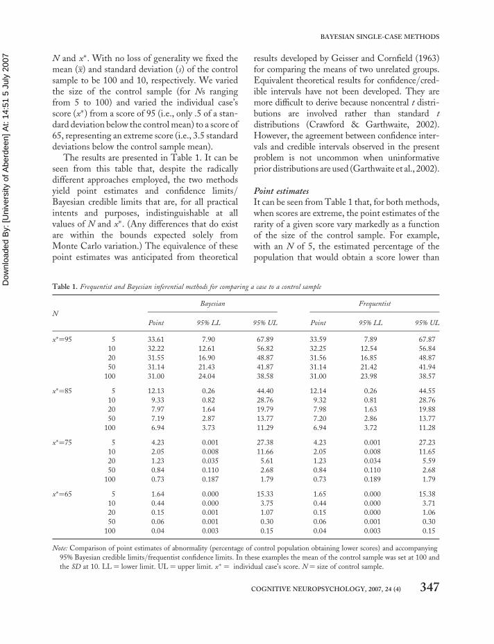
mean (x) and standard deviation (s) of the controlsample to be 100 and 10, respectively. We variedthe size of the control sample (for Ns rangingfrom 5 to 100) and varied the individual case’sscore (x�) from a score of 95 (i.e., only .5 of a stan-dard deviation below the control mean) to a score of65, representing an extreme score (i.e., 3.5 standarddeviations below the control sample mean).

The results are presented in Table 1. It can beseen from this table that, despite the radicallydifferent approaches employed, the two methodsyield point estimates and confidence limits/Bayesian credible limits that are, for all practicalintents and purposes, indistinguishable at allvalues of N and x�. (Any differences that do existare within the bounds expected solely fromMonte Carlo variation.) The equivalence of thesepoint estimates was anticipated from theoretical

results developed by Geisser and Cornfield (1963)for comparing the means of two unrelated groups.Equivalent theoretical results for confidence/cred-ible intervals have not been developed. They aremore difficult to derive because noncentral t distri-butions are involved rather than standard tdistributions (Crawford & Garthwaite, 2002).However, the agreement between confidence inter-vals and credible intervals observed in the presentproblem is not uncommon when uninformativeprior distributions are used (Garthwaite et al., 2002).

Point estimatesIt can be seen from Table 1 that, for both methods,when scores are extreme, the point estimates of therarity of a given score vary markedly as a functionof the size of the control sample. For example,with an N of 5, the estimated percentage of thepopulation that would obtain a score lower than

Table 1. Frequentist and Bayesian inferential methods for comparing a case to a control sample

N

Bayesian Frequentist

Point 95% LL 95% UL Point 95% LL 95% UL

x�¼95 5 33.61 7.90 67.89 33.59 7.89 67.87

10 32.22 12.61 56.82 32.25 12.54 56.84

20 31.55 16.90 48.87 31.56 16.85 48.87

50 31.14 21.43 41.87 31.14 21.42 41.94

100 31.00 24.04 38.58 31.00 23.98 38.57

x�¼85 5 12.13 0.26 44.40 12.14 0.26 44.55

10 9.33 0.82 28.76 9.32 0.81 28.76

20 7.97 1.64 19.79 7.98 1.63 19.88

50 7.19 2.87 13.77 7.20 2.86 13.77

100 6.94 3.73 11.29 6.94 3.72 11.28

x�¼75 5 4.23 0.001 27.38 4.23 0.001 27.23

10 2.05 0.008 11.66 2.05 0.008 11.65

20 1.23 0.035 5.61 1.23 0.034 5.59

50 0.84 0.110 2.68 0.84 0.110 2.68

100 0.73 0.187 1.79 0.73 0.189 1.79

x�¼65 5 1.64 0.000 15.33 1.65 0.000 15.38

10 0.44 0.000 3.75 0.44 0.000 3.71

20 0.15 0.001 1.07 0.15 0.000 1.06

50 0.06 0.001 0.30 0.06 0.001 0.30

100 0.04 0.003 0.15 0.04 0.003 0.15

Note: Comparison of point estimates of abnormality (percentage of control population obtaining lower scores) and accompanying

95% Bayesian credible limits/frequentist confidence limits. In these examples the mean of the control sample was set at 100 and

the SD at 10. LL ¼ lower limit. UL ¼ upper limit. x� ¼ individual case’s score. N ¼ size of control sample.



Dow

nloa

ded

By:

[Uni

vers

ity o

f Abe

rdee

n] A

t: 14

:51

5 Ju

ly 2

007 75 is approximately 4.23%; this is more than four

times the point estimate (0.73%) obtained with acontrol sample of 100 and reflects the greateruncertainty when the control sample is small.

If, as is commonly done in single-case studies,the patient’s score was simply converted to a zscore and evaluated using a table of the normalcurve (i.e., the statistics from the normativesamples were treated as parameters), the pointestimate of the abnormality of this score wouldbe 0.62% regardless of the size of the controlsample. Thus, in the majority of cases, thecommonly used (z score) method will exaggeratethe abnormality of an observed score; when thenormative or control sample is small this effectcan be substantial. Because the Bayesian methodand Crawford and Howell’s (1998) frequentistmethod both treat the control sample statisticsas statistics, they are not subject to thissystematic bias.

Credible limits and confidence limitsThe Bayesian credible limits and frequentist confi-dence limits quantify the degree of uncertaintysurrounding the estimate of the abnormality (i.e.,rarity) of a given test score. It can be seen fromTable 1 that the limits are wide with smallsample sizes. However, even with more moderateNs the limits are not insubstantial and thus serveas a useful reminder of the fallibility of controlor normative data.

Table 1 illustrates another feature of theselimits: They are nonsymmetrical around thepoint estimate. The lower limit (which mustexceed 0; zeros appear in Table 1 only becausethe lower limits in some cases are less than0.001%) is nearer to the point estimate than isthe upper limit. Furthermore, the degree of asym-metry increases the further the case’s score is fromthe mean of the controls.

These asymmetries occur because p follows anoncentral t-distribution. The frequentistapproach (Crawford & Garthwaite, 2002) exploitsthe fact that p follows this distribution in order todetermine confidence limits. However, the fre-quentist method is technically complex and isonly possible at all because the distribution of p

is tractable. In contrast, the Bayesian approachdoes not need to know the distribution of p.

The fact that the two methods yield equivalentlimits means that we can apply a Bayesianinterpretation to either set of limits. Thus, evenif a researcher (or clinician) chose to use the fre-quentist method for this problem, they can legiti-mately avoid the convoluted frequentistinterpretation of these limits. As Antelman(1997) notes, the frequentist (classical) conceptionof a confidence interval is that, “It is one intervalgenerated by a procedure that will give correctintervals 95% of the time. Whether or not theone (and only) interval you happened to get iscorrect or not is unknown” (p. 375).

Thus, in the present context, the frequentistinterpretation is as follows, “if we could computea confidence interval for a large number ofcontrol samples collected in the same way as thepresent control sample, about 95% of themwould contain the true percentage of the popu-lation with scores lower than the patient’s”. Incontrast, the Bayesian analysis shows that it islegitimate to state, “there is a 95% probabilitythat the true level of abnormality of the case’sscore lies within the stated limits”. This statementis not only less convoluted but, we suggest, it alsocaptures what a single-case researcher or clinicianwould wish to conclude from an interval estimate.It is likely that most psychologists who use fre-quentist confidence limits in fact construe thesein what are essentially Bayesian terms (Howell,2002).

The limits presented in Table 1 are two-sidedlimits. However, as noted, one-sided limits arereadily obtained from the Bayesian analysis. Forexample, if a researcher is concerned about howabnormal a case’s score might be, but uninterestedin whether it may be even more unusual than thepoint estimate indicates, then a one-sided upperlimit is more appropriate. Take the example fromTable 1 of the case with a x� of 75 and a controlsample N of 10. Rather than state “There is 95%confidence that the percentage of people whohave a score lower than the patient’s is between0.008% and 11.66%”, we might prefer to state“There is 95% confidence that the percentage of



Dow

nloa

ded

By:

[Uni

vers

ity o

f Abe

rdee

n] A

t: 14

:51

5 Ju

ly 2

007 people who have a score lower than the patient’s is

less than 8.45%”. The latter one-sided upper limitwas obtained by finding the 5,000th largest pi(rather than the 2,500th largest as required fortwo-sided limits; see Method section).

EXPERIMENT 2

Development of a Bayesian analysis forcomparing differences observed in a case todifferences observed in controls

Up to this point we have been concerned with thesimple case of comparing a single test scoreobtained from a patient with a control or norma-tive sample. However, in the assessment ofacquired neuropsychological deficits, simple nor-mative comparison standards have limitationsbecause of the large individual differences in pre-morbid competencies. For example, an averagescore on a test of mental arithmetic is liable to rep-resent a marked decline from the premorbid levelin a patient who was a qualified accountant.Conversely, a score that fell well below the norma-tive mean does not necessarily represent anacquired deficit in an individual who had modestpremorbid abilities (Crawford, 2004; Franzen,Burgess, & Smith-Seemiller, 1997; O’Carroll,1995).

Because of the foregoing, considerable empha-sis is placed on individual comparison standardswhen attempting to detect and quantify the sever-ity of acquired deficits (Crawford, 1992; Lezak,Howieson, Loring, Hannay, & Fischer, 2004;Vanderploeg, 1994). In the simplest case, the neu-ropsychologist may wish to compare an individ-ual’s score on two tests; a fundamentalconsideration in assessing the importance of anydiscrepancy between scores on the two tests isthe extent to which it is rare or abnormal.

The need for a sound method to conduct suchcomparisons is even more acute in single-caseresearch than it is in clinical neuropsychologicalpractice. Although the detection of impairmentsis a fundamental feature of single-case studies, evi-dence of an impairment on a given task usually

only becomes of theoretical interest if it is observedin the context of less impaired or normal perform-ance on other tasks. That is, the aim in manysingle-case studies is to fractionate the cognitivesystem into its constituent parts, and it proceedsby attempting to establish the presence of dis-sociations of function (Caramazza & McCloskey,1988; Crawford, Garthwaite, & Gray, 2003a;Ellis & Young, 1996; Shallice, 1988).

Dissociations have come to play a central role inthe building and testing of theory in cognitiveneuroscience. For example, Dunn and Kirsner(2003) note that, “Dissociations play an increas-ingly crucial role in the methodology of cognitiveneuropsychology . . . they have provided criticalsupport for several influential, almost paradig-matic, models in the field” (p. 2). IndeedRossetti and Revonsuo (2000) have gone as faras to state that “dissociation is the key word ofneuropsychology” (p. 1).

In the typical definition of what is termed aclassical dissociation (Shallice, 1988), the require-ment is that a patient is “impaired” or shows a“deficit” on task X, but is “not impaired”,“normal”, or “within normal limits” on task Y.For example, Ellis and Young (1996) state, “Ifpatient X is impaired on task 1 but performs nor-mally on task 2, then we may claim to have a dis-sociation between tasks” (p. 5). Crawford,Garthwaite, and Gray (2003a) have argued thatthese conventional criteria for a classical dis-sociation should be supplemented by a comparisonof the difference between a patient’s scores on thetwo tasks of interest to the differences on thesetasks observed in the control sample (principallybecause, otherwise, researchers have to rely onthe null result that the patient is not differentfrom controls on one of the tasks).

Striking evidence in favour of this view hasbeen provided by Monte Carlo simulationsstudies (Crawford & Garthwaite, 2005a, 2006a).These studies indicated that high percentages ofthe healthy control population would be incor-rectly classified as exhibiting a dissociation if atest on the case’s difference is not incorporatedinto the criteria. Even higher percentages (over50% in some scenarios) of patients with strictly



Dow

nloa

ded

By:

[Uni

vers

ity o

f Abe

rdee

n] A

t: 14

:51

5 Ju

ly 2

007 equivalent impairments on two tasks would be

misclassified as exhibiting a dissociation (suchpatients are impaired on both tasks but do nothave a dissociation).

Having established the need to compare a case’sdifference score with that of controls, we turn nowto the question of how we should conduct such acomparison. A complication arises because thetasks being compared commonly have differentmeans and standard deviations. The patient’sscores therefore have to be standardized as a com-parison of the raw scores would not be meaningful.Obtaining a sound inferential method of examin-ing the difference between an individual’s standar-dized scores has proved to be much more difficultthan might have been anticipated.

One obvious candidate is the method devel-oped by Payne and Jones (1957): The patient’sscores on the two tasks are converted to z scoresbased on the mean and standard deviations of con-trols, and the difference between them is dividedby the standard deviation of the difference. Theresultant quantity is treated as a standard normaldeviate (zD) and is referred to a table of areasunder the normal curve to estimate the percentageof the control population that would exhibit a dis-crepancy that exceeds the discrepancy observed fora patient.

A number of authors have commented on theusefulness of this formula in neuropsychology(Crawford, 1996; Ley, 1972; Miller, 1993;Shallice, 1979; Silverstein, 1981), and it has beenapplied to the analysis of differences on a varietyof tests (Atkinson, 1991; Grossman, Herman, &Matarazzo, 1985; Mittenberg, Thompson, &Schwartz, 1991). However, just as was the casewith the use of z to compare a single score witha control sample, the Payne and Jones (1957)formula treats the statistics of the normative orcontrol sample as if they were populationparameters.

A Monte Carlo simulation study (Crawford &Garthwaite, 2005b) has demonstrated that thismethod can be associated with very high Type Ierror rates (i.e., it misclassifies a high percentageof the control population as exhibiting an abnor-mal difference); error rates were as high as 25.7%

for a nominal rate of 5% when the controlsample was modest in size. These results demon-strate that the method is only suitable for compari-son of an individual’s standardized difference tothe differences obtained from large normativesamples.

Crawford and Garthwaite (2005b) proposedtwo solutions to this problem. First, they notedthat in some scenarios it is meaningful tocompare the raw difference between two tasksobserved for a case with the raw differences in acontrol sample—that is, it is not always necessaryto standardize the scores. They presented a modi-fied paired-samples t test (which they termed theunstandardized difference test) for this purpose.A Monte Carlo simulation study showed thatthe Type I error rate is under control when thistest is applied regardless of the size of thecontrol sample and magnitude of the correlationbetween the tasks.

Although this approach is sound from a statisti-cal point of view, as noted, it can only be used infairly circumscribed circumstances. It is far morecommon for neuropsychologists to attempt todemonstrate dissociations between tasks of differ-ent cognitive functions in which the two tasks alsohave different means and standard deviations (i.e.,these quantities are essentially often arbitrary). Inthis latter situation it is necessary to standardizethe patient’s score against the control’s perform-ance in order to conduct a meaningful test onthe difference between a patient’s performanceon the two tasks. Therefore it would be veryuseful if a method could be found that permitsstandardization of the patient’s scores whilst alsomaintaining control of the Type I error rate.

Garthwaite and Crawford (2004) determinedthe asymptotic distribution of the differencebetween an individual’s standardized differenceand the standardized differences in controls.They also obtained a test statistic that asymptoti-cally approximates a t-distribution. Monte Carlosimulation studies revealed that the approximationto t was very satisfactory in all scenarios examined(Crawford & Garthwaite, 2005b).

In other words, for the first time a method wasavailable that would control the Type I error rate



Dow

nloa

ded

By:

[Uni

vers

ity o

f Abe

rdee

n] A

t: 14

:51

5 Ju

ly 2

007 when comparing the standardized difference for a

case to the standardized differences for controls (aType I error was defined as misclassifying amember of the control population).1 AlthoughCrawford and Garthwaite suggested that thistest (which they termed the RevisedStandardized Difference Test; RSDT) providesan approximate point estimate of the abnormalityof a case’s score, it did not prove possible usingasymptotic methods to obtain an expression thatwould permit the setting of confidence limits onthe abnormality of a score.

The purpose of the present study was to extendthe Bayesian method developed in Experiment 1to cover examination of score differences in thesingle case. Specifically, (a) we aimed to determinewhether or not a Bayesian approach would exhibitconvergence with Crawford and Garthwaite’s(2005b) frequentist methods of examining unstan-dardized and standardized differences; (b) shouldconvergence not occur, we aimed to explore thereasons for this result; (c) we hoped, for standar-dized differences, to obtain an exact (rather thanapproximate) point estimate of the abnormalityof a case’s difference; and (d) we hoped to solvethe problem of setting credible limits/confidencelimits on the abnormality of such differences.

This last aim is in keeping with the increasingimportance placed on confidence limits by manyscientific bodies including the AmericanPsychological Association (Wilkinson & APATask Force on Statistical Inference, 1999).Confidence limits or credible limits serve theuseful general purpose of reminding us that allresults are fallible and serve the specific purposeof quantifying the degree of uncertainty attachedto a particular result (Crawford & Garthwaite,2002).

Method

We measure the values of x and y on a sample of ncontrols. Let x and y denote the sample means. We

need to form a scale matrix A, which consists ofthe sums-of-squares and cross-products for x andy. In keeping with our aim of requiring thatthese methods can be used when only basicsummary statistics are available for the sample,the elements of this matrix can be obtained fromthe sample standard deviations of x and y (sx, sy)and the sample correlation between x and y (rxy).Let

sxx ¼Xni¼1

(xi � �x)2¼ s2x(n� 1),

syy ¼Xni¼1

(yi � �y)2¼ s2y (n� 1),

and

sxy ¼Xni¼1

(xi � �x)(yi � �y) ¼ sxsyrxy(n� 1):

Put

A ¼sxx sxysxy syy

� �:

We assume each (x, y) comes from a bivariate-normal distribution with unknown mean m ¼ (mx,my)

0 and unknown variance

S ¼sxx sxy

sxy syy

� �:

A case has a value (x�, y�); without loss of gen-erality we assume that x� is greater than y�. Wewant to estimate p, the proportion of controlswhose value of x – y is greater in magnitudethan x� – y�. We also want an interval estimate of p.

We want to start with a standard noninforma-tive prior distribution. For sampling from abivariate normal distribution, as here, there aretwo standard forms of noninformative prior

1 A computer program that implements this test (dissocs.exe), and the unstandardized difference test described earlier, can be

downloaded from http://www.abdn.ac.uk�psy086/dept/SingleCaseMethodsComputerPrograms.HTM



Dow

nloa

ded

By:

[Uni

vers

ity o

f Abe

rdee

n] A

t: 14

:51

5 Ju

ly 2

007 distributions for m and S, either f (m, S�1) / jSj

or f (m, S�1) / jSj3=2. We examined both ofthese priors but here we only report the resultsfor f (m, S�1) / jSj because (as will be seen) itgives classical and Bayesian interval estimatesthat are identical for unstandardized differences.The heuristic motivation for this choice is that fre-quentist methods necessarily ignore prior infor-mation, so presumably a prior distributionconveys no information (i.e., is noninformative)if it leads to Bayesian inferences that are thesame as those given by a frequentist analysis.

The posterior distribution is obtained by com-bining the prior distribution with the data, andinferences and estimates are based on the posteriordistribution. With our choice of prior, the pos-terior distribution states that the marginal distri-bution of S21 is a Wishart distribution withparameters n and A21:

f (S�1) / jS�1j(n�3)=2 exp �

1

2trace(AS�1)

� �:

Given S, the conditional posterior distributionof m is a normal distribution with mean (x, y) andvariance S/n (Geisser & Cornfield, 1963). Thefollowing steps are then followed to obtain esti-mates of p from the posterior distribution:

1. The first step is to generate a random obser-vation (a 2 � 2 matrix in this case) from aninverse-Wishart distribution on n df and scalematrix A. The procedure for generating theserandom observations is set out in Appendix1. Let

S ¼sxx sxy

sxy s yy

� �

denote the generated value. Then S is the esti-mate of S for this iteration.

2. Generate two observations from a standardnormal distribution. Call the generated values(z1, z2). Find the Cholesky decomposition ofS. That is, find the lower triangular matrix T

such that TT 0 ¼ S. Put

mx

m y

� �¼

�x�y

� �þ T

z1

z2

� �=ffiffiffin

p:

Then (mxx, my) is the estimate of m for thisiteration.

3. We have estimates of m and S. We calculate thevalue of p conditional on these being the correctvalues of m and S. At this point the methoddiverges depending upon whether we want toform inferences concerning an individual’sunstandardized or standardized scores on X andY. Considering first the unstandardized case, put

z� ¼(x� � mx) � (y� � my)ffiffiffiffiffiffiffiffiffiffiffiffiffiffiffiffiffiffiffiffiffiffiffiffiffiffiffiffiffiffiffiffiffiffiffiffiffi

(sxx þ s yy � 2sxy)p : (4)

When inferences are to be made concerning anindividual’s standardized scores (as will morecommonly be the case) put

zx ¼x� � mxffiffiffiffiffiffiffi

sxx

p (5)

zy ¼y� � m yffiffiffiffiffiffiffi

s yy

p (6)

and

rxy ¼s yyffiffiffiffiffiffiffiffiffiffiffiffiffiffiffiffiffi

(sxxs yy)p (7)

Then

z� ¼zx � zyffiffiffiffiffiffiffiffiffiffiffiffiffiffiffiffiffiffiffiffi(2 � 2rxy)

q : (8)

4. We find the tail-area of a standard normal dis-tribution that is less than z�. This tail area is anestimate of p, which we call pi for the ithiteration.

5. We repeat Steps 1 to 4 a large number of times;in the present case we perform 100,000



Dow

nloa

ded

By:

[Uni

vers

ity o

f Abe

rdee

n] A

t: 14

:51

5 Ju

ly 2

007 iterations. Then the average value of

p1, . . . , p100,000 is the point estimate of p. (It isthe Bayesian posterior mean of p.) To obtaina 95% Bayesian credible interval, find the2,500th smallest pi and the 2,500th largest pi.Call these values pl and pu. Then the 95%Bayesian credible interval is (pl, pu).

Recall that in Experiment 1 the Bayesianmethod used the familiar formula (3) for a zscore (i.e., a standard score) in computing thepoint and interval estimates for the abnormalityof a case’s score. Analogously, in the present scen-ario, in which we are concerned with obtainingpoint and interval estimates for the abnormalityof the difference between a case’s standardizedscores, the Payne and Jones (1957) formula isused (8). As before, the crucial differencebetween the present approach and the standarduse of the Payne and Jones formula is that, inthe latter case, the sample statistics are pluggeddirectly into the formula. In contrast, with theBayesian approach, these quantities are repeatedlydrawn at random from their posterior distri-butions, thus allowing for their uncertainty.


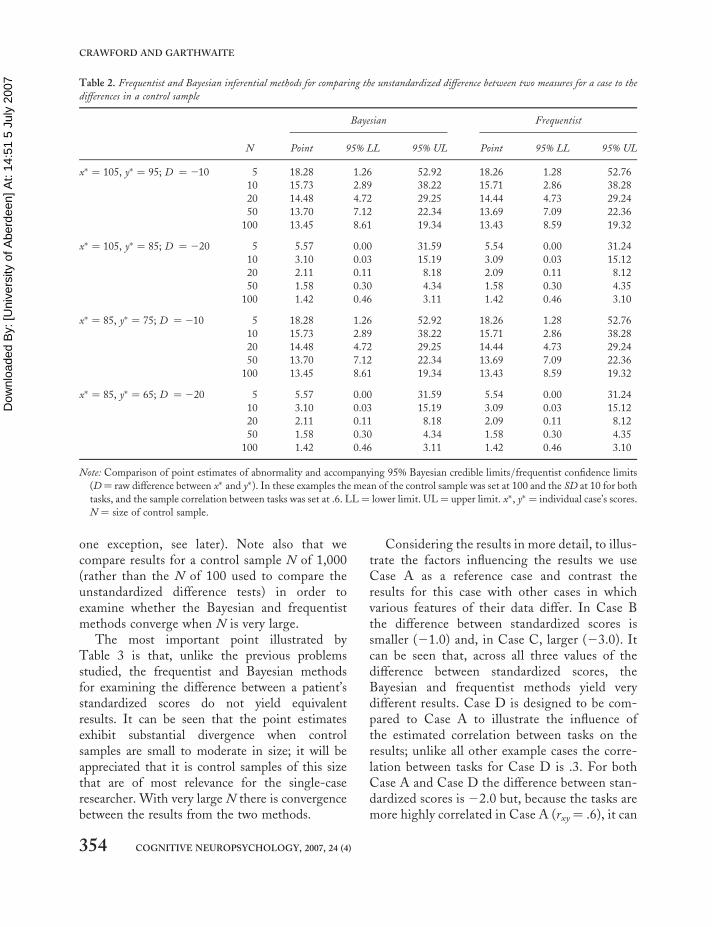
Unstandardized difference for a case compared to thedifferences for controlsIn order to compare the Bayesian and frequentistmethods of comparing the unstandardized differ-ence for a case to those of controls we examinedtheir performance over a range of control sampleNs and correlations between tasks (the correlationsvaried from 0 to .80 but, in the interests ofeconomy, we present results for a correlation of.6 only). Without loss of generality we fixed themeans and standard deviations of the controlsample to be 100 and 10, respectively.

Table 2 reports results for an individual case’s x�

score of 105 (0.5 standard deviations above thecontrol mean) combined with y� scores of either95 (0.5 standard deviations below the controlmean) or 85 (1.5 standard deviations below thecontrol mean). In addition we report results foran individual case’s x� score of 85 combined with

y� scores of 75 or 65. These combinations werechosen so that the raw difference (D in Table 2)was either relatively modest (10) or large (20)and were such that differences could be obtainedby a case whose x� score either was well withinthe normal range or was fairly poor.

It can be seen from Table 2 that the Bayesianand frequentist methods yield equivalent resultswith regard to both the point estimates and theinterval estimates of the abnormality of the case’sscores (again such differences as do exist arewithin the range expected solely from MonteCarlo variation). This equivalence was observedfor other combinations of x� and y� scores andfor the different correlations between the tasks,although these results are not reported here. Theequivalence of the frequentist and Bayesian pointestimates (but not the interval estimates) followsfrom (Geisser & Cornfield, 1963). Note that,should they wish, readers can easily confirm thatequivalence occurs for other values of these vari-ables as the Bayesian unstandardized differencetest has been implemented in a computerprogram (see later section), and the results canbe compared with those from the equivalent fre-quentist program described in Footnote 1.

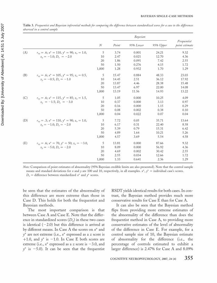
Difference between standardized scores for a casecompared to the differences for controlsA similar procedure to that used to compare theBayesian and frequentist unstandardized differ-ence tests was followed for the standardized differ-ence tests. However, an interval estimate toaccompany the frequentist point estimate is notavailable so there is no equivalent to the Bayesiancredible interval developed in the present paper.With no loss of generality we fixed the meansof the control sample to 100 and standarddeviations to 10.

Results for the Bayesian and frequentistmethods are presented in Table 3. This tablecompares results over a range of control sampleNs and a range of differences between standar-dized scores. We also compared results over arange of correlations between tasks (from 0 to.80) but again, in the interests of economy, wepresent results for a correlation of .6 only (with



Dow

nloa

ded

By:

[Uni

vers

ity o

f Abe

rdee

n] A

t: 14

:51

5 Ju

ly 2

007

one exception, see later). Note also that wecompare results for a control sample N of 1,000(rather than the N of 100 used to compare theunstandardized difference tests) in order toexamine whether the Bayesian and frequentistmethods converge when N is very large.

The most important point illustrated byTable 3 is that, unlike the previous problemsstudied, the frequentist and Bayesian methodsfor examining the difference between a patient’sstandardized scores do not yield equivalentresults. It can be seen that the point estimatesexhibit substantial divergence when controlsamples are small to moderate in size; it will beappreciated that it is control samples of this sizethat are of most relevance for the single-caseresearcher. With very large N there is convergencebetween the results from the two methods.

Considering the results in more detail, to illus-trate the factors influencing the results we useCase A as a reference case and contrast theresults for this case with other cases in whichvarious features of their data differ. In Case Bthe difference between standardized scores issmaller (21.0) and, in Case C, larger (23.0). Itcan be seen that, across all three values of thedifference between standardized scores, theBayesian and frequentist methods yield verydifferent results. Case D is designed to be com-pared to Case A to illustrate the influence ofthe estimated correlation between tasks on theresults; unlike all other example cases the corre-lation between tasks for Case D is .3. For bothCase A and Case D the difference between stan-dardized scores is 22.0 but, because the tasks aremore highly correlated in Case A (rxy ¼ .6), it can

Table 2. Frequentist and Bayesian inferential methods for comparing the unstandardized difference between two measures for a case to the

differences in a control sample

Bayesian Frequentist

N Point 95% LL 95% UL Point 95% LL 95% UL

x� ¼ 105, y� ¼ 95; D ¼ 210 5 18.28 1.26 52.92 18.26 1.28 52.76

10 15.73 2.89 38.22 15.71 2.86 38.28

20 14.48 4.72 29.25 14.44 4.73 29.24

50 13.70 7.12 22.34 13.69 7.09 22.36

100 13.45 8.61 19.34 13.43 8.59 19.32

x� ¼ 105, y� ¼ 85; D ¼ 220 5 5.57 0.00 31.59 5.54 0.00 31.24

10 3.10 0.03 15.19 3.09 0.03 15.12

20 2.11 0.11 8.18 2.09 0.11 8.12

50 1.58 0.30 4.34 1.58 0.30 4.35

100 1.42 0.46 3.11 1.42 0.46 3.10

x� ¼ 85, y� ¼ 75; D ¼ 210 5 18.28 1.26 52.92 18.26 1.28 52.76

10 15.73 2.89 38.22 15.71 2.86 38.28

20 14.48 4.72 29.25 14.44 4.73 29.24

50 13.70 7.12 22.34 13.69 7.09 22.36

100 13.45 8.61 19.34 13.43 8.59 19.32

x� ¼ 85, y� ¼ 65; D ¼ 220 5 5.57 0.00 31.59 5.54 0.00 31.24

10 3.10 0.03 15.19 3.09 0.03 15.12

20 2.11 0.11 8.18 2.09 0.11 8.12

50 1.58 0.30 4.34 1.58 0.30 4.35

100 1.42 0.46 3.11 1.42 0.46 3.10

Note: Comparison of point estimates of abnormality and accompanying 95% Bayesian credible limits/frequentist confidence limits

(D¼ raw difference between x� and y�). In these examples the mean of the control sample was set at 100 and the SD at 10 for both

tasks, and the sample correlation between tasks was set at .6. LL ¼ lower limit. UL ¼ upper limit. x�, y� ¼ individual case’s scores.

N ¼ size of control sample.



Dow

nloa

ded

By:

[Uni

vers

ity o

f Abe

rdee

n] A

t: 14

:51

5 Ju

ly 2

007

be seen that the estimates of the abnormality ofthis difference are more extreme than those inCase D. This holds for both the frequentist andBayesian methods.

The most important comparison is thatbetween Case A and Case E. Note that the differ-ence in standardized scores (Dz) in these two casesis identical (22.0) but this difference is arrived atby different means. In Case A the scores on x� andy� are not extreme (i.e., x� expressed as a z score isþ1.0, and y� is 21.0. In Case E both scores areextreme (i.e., x� expressed as a z score is 23.0, andy� is 25.0). It can be seen that the frequentist

RSDT yields identical results for both cases. In con-trast, the Bayesian method provides much moreconservative results for Case E than for Case A.

It can also be seen that the Bayesian methodflips from providing more extreme estimates ofthe abnormality of the difference than does thefrequentist method in Case A, to providing moreconservative estimates of the level of abnormalityof the difference in Case E. For example, for acontrol sample size of 10, the Bayesian estimateof abnormality for the difference (i.e., thepercentage of controls estimated to exhibit alarger difference) is 2.47% for Case A and 8.09%

Table 3. Frequentist and Bayesian inferential methods for comparing the difference between standardized scores for a case to the differences

observed in a control sample

Bayesian

Frequentist

N Point 95% Lower 95% Upper point estimate

(A) rxy ¼ .6; x� ¼ 110, y� ¼ 90; zx ¼ 1.0,

zy ¼ 21.0; Dz ¼ 22.0

5 3.74 0.001 24.21 9.32

10 2.47 0.021 12.70 4.36

20 1.86 0.091 7.42 2.55

50 1.50 0.276 4.15 1.72

1,000 1.28 0.932 1.70 1.29

(B) rxy ¼ .6; x� ¼ 105, y� ¼ 95; zx ¼ 0.5,

zy ¼ 20.5; Dz ¼ 21.0

5 15.47 0.884 48.33 23.03

10 14.45 2.51 36.12 17.92

20 13.87 4.46 28.38 15.48

50 13.47 6.97 22.00 14.08

1,000 13.19 11.56 14.93 13.22

(C) rxy ¼ .6; x� ¼ 115, y� ¼ 85; zx ¼ 1.5,

zy ¼ 21.5; Dz ¼ 23.0

5 1.05 0.000 10.25 4.09

10 0.37 0.000 3.13 0.97

20 0.16 0.000 1.15 0.29

50 0.08 0.002 0.38 0.10

1,000 0.04 0.022 0.07 0.04

(D) rxy ¼ .3; x� ¼ 110, y� ¼ 90; zx ¼ 1.0,

zy ¼ 21.0; Dz ¼ 22.0

5 7.72 0.05 35.71 13.64

10 6.17 0.31 22.40 8.58

20 5.39 0.79 15.31 6.42

50 4.89 1.64 10.21 5.26

1,000 4.57 3.69 5.54 4.58

(E) rxy ¼ .6; x� ¼ 70, y� ¼ 50; zx ¼ 23.0,

zy ¼ 25.0; Dz ¼ 22.0

5 13.81 0.000 87.66 9.32

10 8.09 0.000 56.92 4.36

20 4.69 0.002 30.42 2.55

50 2.55 0.034 12.66 1.72

1,000 1.33 0.641 2.36 1.29

Note: Comparison of point estimates of abnormality (95% Bayesian credible limits are also presented). Note that the control sample

means and standard deviations for x and y are 100 and 10, respectively, in all examples. x�, y� ¼ individual case’s scores.

Dz ¼ difference between standardized x� and y� scores.



Dow

nloa

ded

By:

[Uni

vers

ity o

f Abe

rdee

n] A

t: 14

:51

5 Ju

ly 2

007 for Case E; the frequentist estimate is 4.36% for

both cases (Table 3).In order to explain the marked differences in

the results for the two methods we need toreturn to the fundamentals of the problem: Wewish to test whether the difference between stan-dardized scores for a case differs from the differ-ences for controls (i.e., we require a hypothesistest). We also wish a point estimate of theabnormality of the case’s difference—that is, wewant to estimate the proportion (or equivalentlythe percentage) of the control population thatwill obtain a more extreme difference in scores.Formally the aim is to examine whether

x� � mx

sx�y� � my

sy

�� (9)

is sufficiently large that scores x�, y� are unlikely tobe the scores of a control. The proportion of thecontrol population with a difference larger thanthat in (9) is

Prx� mx

sx�y � my

sy

�� . x� � mx

sx�y� � my

sy

��

!:

(10)

Using classical frequentist statistics we cannotdetermine this probability. However, it is reason-able to base a significance test on

x� � �x

sx�y� � �y

sy

��: (11)

That is, the sample means and standard devi-ations are substituted for the population meansand standard deviations; note that (11) representsthe (absolute) difference between two t-variates.This was the strategy used by Garthwaite andCrawford (2004) in developing the frequentistRSDT. Specifically, they used asymptotic expan-sion to obtain a test statistic for this differencethat had a distribution that closely approximated at-distribution and controlled the Type I error rate.

In the case of the Bayesian approach to thisproblem we also want to evaluate the probabilityin (9). However, unlike the frequentist approach,with the Bayesian approach we can directly evalu-ate this probability. Moreover, in the previous pro-blems tackled in the present paper the one-tailed pvalue and the point estimate of abnormalitycoincided for both the Bayesian and the frequen-tist approach. In the present case (where we areexamining standardized differences), this doesnot hold for the frequentist approach but doeshold for the Bayesian approach. That is, for theBayesian approach, the proportion of the popu-lation exhibiting a more extreme difference andthe Bayesian p value are one and the same thing.

It follows from the above analysis that we shouldnot expect the frequentist and Bayesian approachesto give the same result, and, given that the latterapproach does not need the pragmatic step of sub-stituting (9) with (11), the Bayesian approach is tobe preferred. (With standardized differences theproblem is too complex for classical methods tohandle easily but, as previously noted, Bayesianmethods can handle more complex problems thancan classical methods.)

Further consideration of the nature of thedifferences in results for the two approaches pro-vides a further insight. This is best illustrated bymaking further use of the examples provided byCases A and E in Table 3. Because the differencebetween standardized scores is the same in thesetwo cases, the frequentist standardized differencetest gives identical p-values. However, error inestimating a standard deviation will have agreater effect in Case E than in Case A becausethe standard deviations divide larger quantities inCase E than in Case A. To illustrate, imaginethat the standard deviation for y was 9rather than 10. Then the difference betweenstandardized scores for Case A would be(þ1.0) 2 (21.111) ¼ 22.111, while for CaseE it would be (23.0) 2 (25.556) ¼ 22.556.It can be seen that the modest change in the stan-dard deviation of y has had a substantial effect onCase E’s z score for y� and hence a substantialeffect on the difference between standardizedscores; the effect on Case A is much less



Dow

nloa

ded

By:

[Uni

vers

ity o

f Abe

rdee

n] A

t: 14

:51

5 Ju

ly 2

007 marked. If the standard deviation of y was 11

rather than 10 then again we see that the effecton Case E is much more pronounced—that is,the difference between z scores for this case isthen 21.545 whereas it is 21.909 for Case A.

The frequentist standardized difference testlooks only at the estimated difference betweenthe standardized scores and so ignores the individ-ual differences in x and y. In contrast, the Bayesiantest factors in the greater uncertainty in Case Eand so will not yield the same answer for the twocases; for Case E, the Bayesian estimate of theabnormality of the difference will, appropriately,be less extreme.

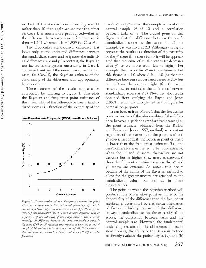
These features of the results can also beappreciated by referring to Figure 1. This plotsthe Bayesian and frequentist point estimates ofthe abnormality of the difference between standar-dized scores as a function of the extremity of the

case’s x� and y� scores; the example is based on acontrol sample N of 10 and a correlationbetween tasks of .6. The crucial point in thisfigure is that the difference between the case’sstandardized scores is the same for all theexamples; it was fixed at 2.0. Although the figurepresents the results as a function of the extremityof the y� score (in z score form) it will be appreci-ated that the value of x� also varies (it decreaseswith y� as we move from left to right). Forexample, the z score for x� on the extreme left ofthis figure is þ1.0 when y� is 21.0 (so that thedifference between standardized scores is 2.0) butis 24.0 on the extreme right (for the samereason, i.e., to maintain the difference betweenstandardized scores at 2.0). Note that the resultsobtained from applying the Payne and Jones(1957) method are also plotted in this figure forcomparison purposes.

It can be seen from Figure 1 that the frequentistpoint estimates of the abnormality of the differ-ence between a patient’s standardized scores (i.e.,the point estimates obtained from the RSDTand Payne and Jones, 1957, method) are constantregardless of the extremity of the patient’s x� andy� scores. In contrast, the Bayesian point estimateis lower than the frequentist estimates (i.e., thecase’s difference is estimated to be more extreme)when the x� and y� scores themselves are notextreme but is higher (i.e., more conservative)than the frequentist estimates when the x� andy� scores are extreme. As noted, this occursbecause of the ability of the Bayesian method toallow for the greater uncertainty attached to thestandardized values zx and zy in thesecircumstances.

The point at which the Bayesian method willproduce more conservative point estimates of theabnormality of the difference than the frequentistmethods is determined by a complex interactionof factors including the size of the differencebetween standardized scores, the extremity of thescores, the correlation between tasks and thecontrol sample size. However, the fundamentalunderlying reasons for the differences in resultsstem from (a) the ability of the Bayesian methodto directly evaluate the probability in (9), and (b)

Figure 1. Demonstration of the divergence between the point

estimates of abnormality (i.e., estimated percentage of controls

exhibiting a larger difference than the single case) for the Bayesian

(BSDT) and frequentist (RSDT) standardized difference tests as

a function of the extremity of the single case’s x and y scores;

crucially, the difference between the case’s standardized scores is

the same (2.0) in all examples (the example is based on a control

sample of 20 and correlation between tasks of .6). Point estimates

obtained from the method of Payne and Jones (1957) are also

presented.



Dow

nloa

ded

By:

[Uni

vers

ity o

f Abe

rdee

n] A

t: 14

:51

5 Ju

ly 2

007 the fact that it differentiates between a case for

which both x� and y� are extreme and a case inwhich x� and y� are less extreme, even thoughthe magnitude of the difference between theirstandardized scores is the same.

This latter feature of the Bayesian methodmakes it particularly suitable for use in single-case research in neuropsychology. As noted, ifthe aim of a single-case study is to demonstrate a(classical) dissociation, the Monte Carlo simu-lation studies provide striking evidence that atest on the difference between a single-case’sscores should be performed (Crawford &Garthwaite, 2005a). Without such a test—thatis, if a researcher demonstrates only that thepatient’s performance on task y is significantlybelow controls whereas performance on task x isnot significantly lower (i.e., is “within normallimits”)—the chances are high that the apparentdissociation will be spurious.

Furthermore, in neuropsychological single-caseresearch, evidence of what have been termed“strong dissociations” (Shallice, 1988) is alsoused as evidence for modularity (Coltheart,2001). In such cases it is necessarily the case thatthe scores of the single case are extreme on bothtasks (i.e., their performance on both tasks was suf-ficiently low to conclude that they were impairedon both tasks). Thus, the Bayesian test willprovide a more rigorous means of testing for astrong dissociation than any of the available fre-quentist methods. This is an important practicaladvantage for the Bayesian method as cases withstrong dissociations are more likely to be encoun-tered than cases with classical dissociations(Crawford & Garthwaite, 2006a).

In conclusion, the frequentist and Bayesianapproaches to the analysis of a case’s standardizeddifference will not yield equivalent results. TheBayesian analysis has a number of advantagesover its frequentist alternative. First, it can directlyevaluate the probability required, rather than esti-mate it second hand. Second, the Bayesian testwill, appropriately, yield a more conservativeresult when the x� or y� scores are extreme(because extreme scores will be more sensitive toerror in estimating the control standard

deviations). In contrast, the frequentist approachwill not capture the differing level of uncertaintyattached to estimating the standard deviations.As noted, this feature makes the Bayesianmethod particularly useful in neuropsychologicalapplications. Third, a very appealing feature ofthe Bayesian method is that the p value simul-taneously provides an exact point estimate of theabnormality of the difference. In contrast, the fre-quentist p value cannot serve this dual function(although, as noted, frequentist p values do servethis dual function for the earlier problemsstudied in the present paper). Fourth, in previouswork by the present authors (Garthwaite &Crawford, 2004), it did not prove possible toobtain frequentist interval estimate of the abnorm-ality of a standardized difference whereas this isreadily achieved with the Bayesian method.

EXPERIMENT 3

Monte Carlo simulation of Type I errors forfrequentist and Bayesian methods of testingfor a standardized difference

In this study a Monte Carlo simulation is per-formed to further evaluate the frequentist andBayesian methods for examining standardizeddifferences. The aim was to study the Type Ierror rate for these methods; in this context aType I error occurs when we falsely concludethat the difference between a case’s standardizedscores is not an observation from the correspond-ing differences in the control population—thatis, we claim that the case’s difference is abnormalwhen it is not. Note that, when the interest in asingle-case study is in the difference between anindividual’s performance on two tasks, one candefine two forms of Type I error. The most funda-mental occurs when a healthy (i.e., cognitivelyintact) control is misclassified. However, asecond form of error can also occur—namely, mis-classifying a patient with an equivalent level ofacquired impairment on two tasks as exhibitingan abnormal standardized difference. In practice,the latter form of Type I error will be much



Dow

nloa

ded

By:

[Uni

vers

ity o

f Abe

rdee

n] A

t: 14

:51

5 Ju

ly 2

007 more of a threat to validity than the former

(Crawford & Garthwaite, 2006a) and is theprimary focus of the present study. The methodadopted is based on an approach used byCrawford and Garthwaite (2005a) in which con-trols and a single case are sampled from the samecontrol distribution but the case is then “lesioned”to impose strictly equal impairments on the twotasks.

It should be stressed that this simulation isbased on the frequentist approach to statistics.With this approach, the question of interest is“If these are the values of my population par-ameters, what data values would be observed?” Inthe simulations the parameter values are indeedfixed, and data are being generated and observed.The Bayesian approach asks the question “Ifthese are the values of the data, what valuesmight the parameters take?” That is, in theBayesian approach the data values are fixed, andthe population parameters are the variable quan-tity. Hopefully, good methods of inference willgenerally perform reasonably well under most sen-sible criteria, rather than just the criteria for whichthey were designed. This simulation examines howthe Bayesian method of testing for a dissociationperforms under a frequentist criterion.

Method

The Monte Carlo simulation was run on a PC andimplemented in Borland Delphi (Version 4). Thealgorithm ran3.pas (Press, Flannery, Teukolsky, &Vetterling, 1989) was used to generate uniformrandom numbers (between 0 and 1), and thesewere transformed by the polar variant of theBox–Muller method (Box & Muller, 1958). TheBox–Muller transformation generates pairs ofnormally distributed observations, and, by furthertransforming the second of these, it is possible togenerate observations from a bivariate normaldistribution with a specified correlation (e.g., seeKennedy & Gentle, 1980).

The simulation was run with two differentvalues of N (the sample size of the controlsample): 10 and 20 (these are fairly typical Ns insingle-case research, although even smaller Ns

are not uncommon). For each of these values ofN, 10,000 samples of N þ 1 were drawn fromone of two bivariate normal distributions inwhich the population correlation (rXY) was set ateither .3 or .6.

In each trial, the first N pairs of observationswere taken as the control sample’s scores on x andy, and the (N þ 1)th pair was taken as the premor-bid scores of the single case. The single case wasthen “lesioned” by imposing an acquired impair-ment of a specified number of standard deviations(1, 2, 4, 6, and 8) on both x� and y�. (An impair-ment of 8 standard deviations is clearly extremelysevere but not beyond the bounds of possibilitygiven the catastrophic effects of some cerebrallesions.) As the observations are sampled from astandard normal bivariate distribution, the standarddeviation is 1.0 for both tasks x and y. Hence therequired impairments are achieved simply by sub-tracting 1, 2, 4, 6, or 8 from the x� and y� scoresof the single case. These cases are used to representpatients who had suffered strictly equal deficits on xand y. Thus, if any of the statistical methods recorda difference between x� and y� for such cases, thisconstitutes a Type I error.

Note that, although this procedure is designedto model patients with identical acquired deficits,it does not produce cases with identical scores onx and y. Rather, the method recognizes that, (a)patients are initially members of the healthycontrol population until the onset of their lesion,(b) there will be premorbid differences in compe-tencies on x and y, and (c) the magnitude of pre-morbid differences between x and y will be afunction of the population correlation betweenthe two tasks (i.e., the magnitude of such differ-ences will, on average, be smaller when the popu-lation correlation is high than when it is low). Thestandardized scores (zx and zy) will also be affectedby random variation in estimating the populationmeans and standard deviations.

The simulations also contained a condition inwhich no (zero) impairments were imposed onthe cases’ scores; these cases represent healthycontrol cases.

In total 240,000 Monte Carlo trials were run—that is, 10,000 trials for each combination of the



Dow

nloa

ded

By:

[Uni

vers

ity o

f Abe

rdee

n] A

t: 14

:51

5 Ju

ly 2

007 two sample sizes (10 and 20), the two values for

the population correlation (.3 and .6), and the sixlevels of acquired impairment (this includesacquired impairments of zero as noted above).The number of Monte Carlo trials were limitedto 10,000 per condition because of the computa-tionally intensive nature of the simulations; thatis, on each trial the Bayesian StandardizedDifference Test (BSDT) was applied to thescores of the single case, and (as noted inExperiment 2) this required a further 100,000Monte Carlo trials per case.

On each Monte Carlo trial the three statisticalmethods (the BSDT, the frequentist RSDT, andthe Payne and Jones, 1957, method) wereapplied to the scores of the single case using aspecified Type I error rate of 5% for all threemethods. A Type I error was recorded for thePayne and Jones method when z for the differencebetween the case’s standardized scores exceeded1.946; for the frequentist RSDT a Type I errorwas recorded when t exceeded the critical valuefor t on n 2 2 df; a Type I error was recordedfor the Bayesian test, when the mean p valuefrom the 100,000 iterations was below .05. Thenumber of Type I errors for each method werethen expressed as a percentage of the totalnumber of trials in each condition.


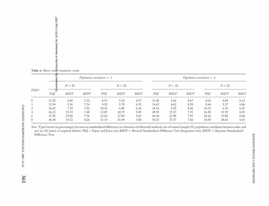
The full results from the simulation are presentedin Table 4. In addition, the results are presentedgraphically in Figure 2 but are limited to thoseresults obtained for a control sample size of 20and population correlation of .6.

The first thing to note is that, despite its wide-spread use, the Payne and Jones (1957) methodachieves very poor control over Type I errors inall scenarios. Compared to the specified errorrate of 5%, the minimum Type I error rate was8.32% (when no impairments were present, thecontrol sample size was 20, and correlationbetween tasks was .6), and the maximum errorrate was 50.15% (for impairments of 8 standarddeviations, the control sample size was 10, andcorrelation was .6).

Turning to the two more serious contenders, itcan be seen that the RSDT yields Type I errorrates that are nearer to 5% than the Bayesian testwhen impairments on x� and y� are either absent(i.e., impairment ¼ 0) or mild (i.e., 1 SD). Toillustrate the differences in results for the twomethods: The error rate for a control sample sizeof 20, correlation between tasks of .3, and acquiredimpairments of 1 standard deviation is 5.70% forthe RSDT but is 6.52% for the Bayesian test.Thereafter, however, the error rates for theRSDT increasingly exceed those of the Bayesiantest as the cases’ impairments on x� and y�

become more extreme; as can be seen fromTable 4, the error rate was as high as 37.57% forthe RSDT (for a control sample size of 10, corre-lation between tasks of .6, and impairments of 8SDs). In contrast, the Bayesian error rates aremuch lower; the maximum error rate is 8.67%(for a control sample size of 10, correlation of .6,and zero impairments). It can also be seen thatthe Type I error rate for the Bayesian test isfairly consistent across the varying levels of theextremity of the x� and y� scores (in keepingwith the fact that it allows for the extremity ofthese scores thereby requiring a larger standar-dized difference before p falls below .05 thanthat required when the scores are less extreme).

It must be stressed that the foregoing simu-lation is based on the frequentist approach as ineach group of simulations the parameter valueswere fixed at one set of values, and many differentsets of data were generated. With the Bayesianapproach, in one group of simulations the datawould be fixed at one set of values, and manydifferent values of the population parameterswould be generated. The results show that theBayesian method performs well under the fre-quentist criteria and, indeed, much better thanthe frequentist method does when the x and yscores of the case are extreme. Whether the fre-quentist method performs well under theBayesian criterion would depend upon the datain hand, performing poorly if the case’s x and yscores are extreme.

In summary, the simulation, despite beingbased on frequentist assumptions, supports the



Dow

nloa

ded

By:

[Uni

vers

ity o

f Abe

rdee

n] A

t: 14

:51

5 Ju

ly 2

007

Table 4. Monte Carlo simulation results

Population correlation ¼ .3 Population correlation ¼ .6

Deficit

N ¼ 10 N ¼ 20 N ¼ 10 N ¼ 20

P&J RSDT BSDT P&J RSDT BSDT P&J RSDT BSDT P&J RSDT BSDT

0 11.92 4.68 7.32 8.57 5.30 6.57 13.42 5.60 8.67 8.32 4.84 6.12

1 12.94 5.36 7.34 9.20 5.70 6.52 14.63 6.62 8.58 8.46 5.37 6.06

2 16.05 7.29 7.02 10.41 6.80 6.36 18.16 9.20 8.26 10.32 6.33 6.07

4 26.13 15.33 7.48 15.85 10.79 5.89 28.93 17.27 7.93 16.98 11.95 6.05

6 37.25 25.05 7.76 23.60 17.82 5.65 40.42 27.90 7.97 25.63 19.80 6.06

8 46.48 34.72 8.26 31.35 25.49 5.80 50.15 37.57 7.82 34.58 28.65 6.03

Note : Type I errors (as percentages) for tests on standardized differences as a function of inferential method, size of control sample (N), population correlation between tasks, and

size (in SD units) of acquired deficits. P&J ¼ Payne and Jones test; RSDT ¼ Revised Standardized Difference Test (frequentist test); BSDT ¼ Bayesian Standardized

Difference Test.

COGNIT

IVENEUROPSYCHOLOGY,2007,24(4)

361

BAYESIA

NSIN

GLE-C

ASEM

ETHODS

Dow

nloa

ded

By:

[Uni

vers

ity o

f Abe

rdee

n] A

t: 14

:51

5 Ju

ly 2

007

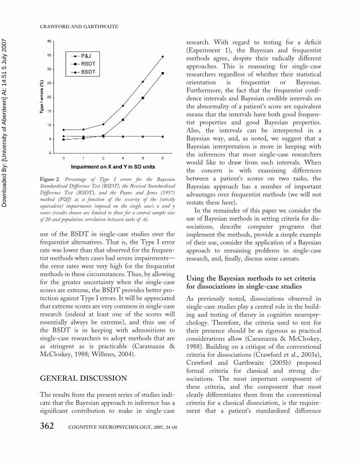
use of the BSDT in single-case studies over thefrequentist alternatives. That is, the Type I errorrate was lower than that observed for the frequen-tist methods when cases had severe impairments—the error rates were very high for the frequentistmethods in these circumstances. Thus, by allowingfor the greater uncertainty when the single-casescores are extreme, the BSDT provides better pro-tection against Type I errors. It will be appreciatedthat extreme scores are very common in single-caseresearch (indeed at least one of the scores willessentially always be extreme), and thus use ofthe BSDT is in keeping with admonitions tosingle-case researchers to adopt methods that areas stringent as is practicable (Caramazza &McCloskey, 1988; Willmes, 2004).

GENERAL DISCUSSION

The results from the present series of studies indi-cate that the Bayesian approach to inference has asignificant contribution to make in single-case

research. With regard to testing for a deficit(Experiment 1), the Bayesian and frequentistmethods agree, despite their radically differentapproaches. This is reassuring for single-caseresearchers regardless of whether their statisticalorientation is frequentist or Bayesian.Furthermore, the fact that the frequentist confi-dence intervals and Bayesian credible intervals onthe abnormality of a patient’s score are equivalentmeans that the intervals have both good frequen-tist properties and good Bayesian properties.Also, the intervals can be interpreted in aBayesian way, and, as noted, we suggest that aBayesian interpretation is more in keeping withthe inferences that most single-case researcherswould like to draw from such intervals. Whenthe concern is with examining differencesbetween a patient’s scores on two tasks, theBayesian approach has a number of importantadvantages over frequentist methods (we will notrestate these here).

In the remainder of this paper we consider theuse of Bayesian methods in setting criteria for dis-sociations, describe computer programs thatimplement the methods, provide a simple exampleof their use, consider the application of a Bayesianapproach to remaining problems in single-caseresearch, and, finally, discuss some caveats.

Using the Bayesian methods to set criteriafor dissociations in single-case studies

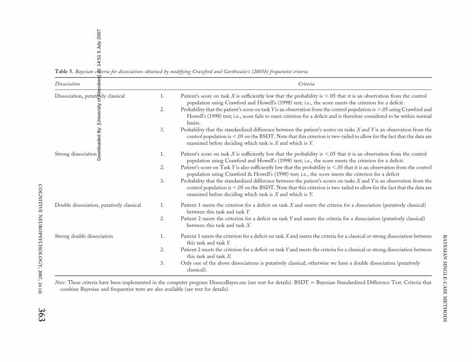
As previously noted, dissociations observed insingle-case studies play a central role in the build-ing and testing of theory in cognitive neuropsy-chology. Therefore, the criteria used to test fortheir presence should be as rigorous as practicalconsiderations allow (Caramazza & McCloskey,1988). Building on a critique of the conventionalcriteria for dissociations (Crawford et al., 2003a),Crawford and Garthwaite (2005b) proposedformal criteria for classical and strong dis-sociations. The most important component ofthese criteria, and the component that mostclearly differentiates them from the conventionalcriteria for a classical dissociation, is the require-ment that a patient’s standardized difference

Figure 2. Percentage of Type I errors for the Bayesian

Standardized Difference Test (BSDT), the Revised Standardized

Difference Test (RSDT), and the Payne and Jones (1957)

method (P&J) as a function of the severity of the (strictly

equivalent) impairments imposed on the single case’s x and y

scores (results shown are limited to those for a control sample size

of 20 and population correlation between tasks of .6).



Dow

nloa

ded

By:

[Uni

vers

ity o

f Abe

rdee

n] A

t: 14

:51

5 Ju

ly 2

007

Table 5. Bayesian criteria for dissociations obtained by modifying Crawford and Garthwaite’s (2005b) frequentist criteria

Dissociation Criteria

Dissociation, putatively classical 1. Patient’s score on task X is sufficiently low that the probability is ,.05 that it is an observation from the control

population using Crawford and Howell’s (1998) test; i.e., the score meets the criterion for a deficit.

2. Probability that the patient’s score on task Y is an observation from the control population is ..05 using Crawford and

Howell’s (1998) test; i.e., score fails to meet criterion for a deficit and is therefore considered to be within normal

limits.

3. Probability that the standardized difference between the patient’s scores on tasks X and Y is an observation from the

control population is ,.05 on the BSDT. Note that this criterion is two-tailed to allow for the fact that the data are

examined before deciding which task is X and which is Y.

Strong dissociation 1. Patient’s score on task X is sufficiently low that the probability is ,.05 that it is an observation from the control

population using Crawford and Howell’s (1998) test; i.e., the score meets the criterion for a deficit.

2. Patient’s score on Task Y is also sufficiently low that the probability is ,.05 that it is an observation from the control

population using Crawford & Howell’s (1998) test; i.e., the score meets the criterion for a deficit

3. Probability that the standardized difference between the patient’s scores on tasks X and Y is an observation from the

control population is ,.05 on the BSDT. Note that this criterion is two-tailed to allow for the fact that the data are

examined before deciding which task is X and which is Y.

Double dissociation, putatively classical 1. Patient 1 meets the criterion for a deficit on task X and meets the criteria for a dissociation (putatively classical)

between this task and task Y.

2. Patient 2 meets the criterion for a deficit on task Y and meets the criteria for a dissociation (putatively classical)

between this task and task X.

Strong double dissociation 1. Patient 1 meets the criterion for a deficit on task X and meets the criteria for a classical or strong dissociation between

this task and task Y.

2. Patient 2 meets the criterion for a deficit on task Y and meets the criteria for a classical or strong dissociation between

this task and task X.

3. Only one of the above dissociations is putatively classical; otherwise we have a double dissociation (putatively

classical).

Note: These criteria have been implemented in the computer program DissocsBayes.exe (see text for details). BSDT ¼ Bayesian Standardized Difference Test. Criteria that

combine Bayesian and frequentist tests are also available (see text for details).

COGNIT

IVENEUROPSYCHOLOGY,2007,24(4)

363

BAYESIA

NSIN

GLE-C

ASEM

ETHODS

Dow

nloa

ded

By:

[Uni

vers

ity o

f Abe

rdee

n] A

t: 14

:51

5 Ju

ly 2

007 between tasks x and y should be sufficiently large to

render it unlikely (p, .05) that it is an observationfrom the standardized differences in the controlpopulation. These criteria were all based on theapplication of frequentist statistical methods (i.e.,Crawford and Howell’s, 1998, test was used totest for a deficit on tasks x and y, and the RSDTwas used to test the standardized differencebetween the two tasks).

The methods developed in the present paperallow us to develop criteria for dissociationsbased on the results from Bayesian analysis ofthe scores of the single case. The essential featuresof these criteria are broadly the same as their fre-quentist counterparts. Indeed, given that theBayesian test for a deficit (BTD) has been shownto yield equivalent results to Crawford andHowell’s (1998) frequentist test,2 the only sub-stantive difference is the use of the Bayesian stan-dardized difference test (BSDT) in place of thefrequentist Revised Standardized DifferenceTest. The formal Bayesian criteria for dissociationsare presented in Table 5.

Note that in developing these criteria we adoptCrawford and Garthwaite’s (2006a) suggestedchange to nomenclature in that, although weretain the term “strong dissociation”, we replacethe term “classical dissociation” with “a dis-sociation, putatively classical”. Crawford andGarthwaite (2006a) argued for this change onthe basis of the results from Monte Carlo simu-lations studies. These studies indicated that,although one can have a high degree of confidencethat a patient identified as exhibiting a classicaldissociation has some form of dissociation, onecannot have a similar degree of confidence that itis classical in form; many patients who in realityhave a strong dissociation will be classified as exhi-biting a classical dissociation because the deficit onthe less impaired of the two tasks will frequentlynot be detected. In contrast (provided that

Crawford and Garthwaite’s criteria are used), apatient with a genuine classical dissociation willrarely be classified as exhibiting a strong dis-sociation, thereby suggesting that the cautionaryterm “putative” is not necessary in the case ofstrong dissociations. This should not be inter-preted as suggesting that there is no uncertaintywith the former form of dissociation; the differ-ence in nomenclature is used to flag that thedegree of uncertainty is substantially greater inthe case of classical dissociations.

In addition to developing purely Bayesian cri-teria for a dissociation, it is also possible to usethe Bayesian methods to develop criteria thatwould satisfy those single-case researchers who arefirmly frequentist in their orientation. That is, inthe presence of extreme acquired impairments onthe two tasks, the BSDT performs better than thefrequentist tests when evaluated against frequentistassumptions. Thus a “belt and braces” approach toidentifying dissociations could be adopted inwhich the BSDT and the frequentist RSDT areapplied to the difference between a patient’s stan-dardized scores and a dissociation recorded onlywhen p is less than .05 on both tests. The RSDTwould provide reassurance for frequentists whenthe acquired impairments are mild (as Type Ierrors are lower for the RSDT in these circum-stances), and the BSDT provides cover againsterror when the acquired impairments are extreme.(Note that, for a given single case, we cannotknow whether scores that are only moderatelylower than the control mean represent a mildimpairment or severe impairment because wecannot know the premorbid level of competency.)

Computer programs to implement theBayesian methods

The methods developed in the present paper couldbe implemented in Bayesian analysis programs

2 Crawford and Howell’s (1998) test for a deficit is used for computational convenience in setting these criteria. That is, a com-

puter program is available to test whether a case meets these criteria (see General Discussion section for details). Use of Crawford and

Howell’s test, rather than the equivalent Bayesian test for a deficit, means that only one set of 100,000 observations need be sorted (to

obtain credible limits on the abnormality of the standardized difference) rather than three sets (two further sorts would be required to

obtain the limits on the abnormality of the case’s x and y scores).



Dow

nloa

ded

By:

[Uni

vers

ity o

f Abe

rdee

n] A

t: 14

:51

5 Ju

ly 2

007 such as BUGS (Spiegelhalter, Thomas, Best, &

Gliks, 1996). However, a reasonable level of tech-nical skill would be required. As we are aware thatmany researchers and practitioners may haveneither the skills nor the time to pursue theseoptions, we have written programs (for PCs) thatare specifically tailored to implementing thepresent Bayesian inferential methods.

A very useful and convenient feature of theseprograms (and indeed, more generally, of themethods themselves) is that they require only thesummary statistics for the control sample ratherthan the raw data. Armed with these programs asingle-case researcher (or clinician) can enter therequisite data and obtain the relevant results inunder a minute (given the computer intensivenature of the analysis, this is a testament to thespeed of modern bulk standard PCs).

The program SingleBayes.exe implements theBayesian test for a deficit derived in Experiment 1.The data inputs required are the control samplemean and standard deviation for the task of interest,the control sample N, and the patient’s score. Theoutput consists of the one- and two-tailed Bayesianp value, the point estimate of the abnormality of theindividual’s score, and the 95% Bayesian credibleinterval on this percentage. By default thecredible interval is two-sided but a one-sided upperor lower limit can be selected if required (see earlierdiscussion on the use of one-sided limits inExperiment 1).

The program DiffBayes.exe implements theBayesian methods for comparing a case’s differ-ence against the differences in controls. Thisprogram prompts the user to select either theBayesian unstandardized difference test (BUDT)or Bayesian standardized difference test (BSDT).The data inputs required are the means and stan-dard deviations for both tasks and their correlationin the control sample, the N for the controlsample, and the patient’s scores.

The results of applying the selected differencetest are reported: namely, the two-tailed prob-ability; the point estimate of the abnormality ofthe patient’s difference (i.e., the estimatedpercentage of the control population that wouldexhibit a more extreme discrepancy); and the

95% Bayesian credible interval for this percentage.As is the case for SingleBayes.exe, by defaultthe credible interval is two-sided but a one-sided upper or lower limit can be selected ifrequired.

The program DissocsBayes.exe implements thecriteria for dissociations set out in Table 4 and dis-cussed in the previous section. That is, it tests for adeficit on task x and task y using Crawford andHowell’s (1998) test (which, as noted, is equivalentto the Bayesian test for a deficit) and tests the stan-dardized difference using the BSDT. The patternof results from applying these tests determineswhether the patient meets the criteria for astrong dissociation or a dissociation (putativelyclassical).

It was noted in the previous section that theBSDT could also be combined with use of the fre-quentist RSDT to provide combined criteria fordissociations that would satisfy those of afirmly frequentist orientation. The DissocsBayesprogram also applies these combined criteria.That is, when the combined criteria are used, a dis-sociation is only recorded when the p values fromboth the BSDT and RSDT are below .05. In allother respects these criteria are the same as thoseset out in Table 5; that is, a strong dissociation isrecorded when the patient’s performance on bothtasks qualify as deficits, and a dissociation (puta-tively classical) is recorded if only one of thetasks qualifies as deficit. The data inputs requiredfor DissocsBayes.exe are the same as those forDiffBayes.exe: namely, the means and standarddeviations for both tasks and their correlation inthe control sample, the N for the control sample,and the patient’s scores.

The results generated by these three programscan be viewed on screen, printed, or saved to afile. In addition, the statistics for the controlsample are reloaded when the programs are re-run making it convenient to run analyses onfurther cases (alternatively, the control data canbe cleared). The fact that the methods andprograms that implement them require onlythe summary data for the controls also meansthat analysis can be run using previously publishedcontrol data or control data from a third party. The



Dow

nloa

ded

By:

[Uni

vers

ity o

f Abe

rdee

n] A

t: 14

:51

5 Ju

ly 2

007 programs can be downloaded from: www.abdn.

ac.uk/�psy086/dept/BayesSingleCase.htm

An examples of the use of the Bayesianmethods

To illustrate the use of the Bayesian methods,suppose that a researcher administered a theoryof mind (ToM; Baron-Cohen, Leslie, & Frith,1985) task and a task of executive ability (e.g.,set shifting) to a patient. The researcher wants toassess whether there is evidence of deficits oneither or both of the two tasks and wishes to deter-mine whether there was an abnormal differencebetween the two tasks (i.e., they wish to estimatethe probability that the difference observed forthe patient was drawn from the distribution ofdifferences in the control population).Ultimately, the researcher is interested in assessingwhether the patient exhibits a dissociationbetween ToM and executive ability and, ifso, whether this dissociation is putativelyclassical in form or is best regarded as a strongdissociation.

Suppose also that 20 healthy controls matchedto the patient on basic demographic variableshave been recruited. The mean score for controlson the ToM task was 60 (SD ¼ 7.0), and themean score on the executive task was 24 (SD ¼

4.8); the correlation between the two tasks in con-trols was .68. Finally, suppose the patient’s rawscores on these two tasks were 33 and 15,respectively.

Applying the Bayesian test for a deficit (BTD)to the patient’s ToM score, it is estimated that only0.067% of the control population would obtain ascore lower than the patient’s (i.e., this is thepoint estimate of the abnormality of the score),and the accompanying 95% credible interval onthis quantity is from ,0.0001% to 0.54%. As thepoint estimate tells us that less than 5% of thecontrol population are expected to score lowerthan the patient, the score meets the criteria fora deficit; that is, the null hypothesis, that thescore is an observation from the control popu-lation, is rejected (p , .05, one-tailed). If aresearcher considered that the suggested criterion

is overly liberal they need only modify it torequire a more extreme point estimate ofabnormality.

Turning to the patient’s score on the executivetask, it is estimated that 4.15% of the controlpopulation would exhibit a lower score (95% CI¼ 0.47% to 12.95%), and thus it is concludedthat the patient also exhibits a deficit (p , .05,one-tailed) on the executive task. The patient’sscores on the ToM task and executive taskexpressed as z scores are 2 3.857 and 2 1.875,respectively; the impairment on the ToM task isgreater than that on the executive tasks but thequestion remains of whether this differencebetween the standardized scores is abnormal.That is, what is the probability that thisdifference is an observation from the control popu-lation? Application of the Bayesian standardizeddifference test addresses this question: The prob-ability is .043. Note that this probability is two-tailed in that it is based on the absolute differencebetween the patient’s standardized scores (i.e., itestimates the probability that a member of thecontrol population would exhibit a larger differ-ence in either direction). The Bayesian test alsoprovides a point estimate of the percentage ofthe control population that would exhibit alarger difference in the same direction as the case’sdifference. In this example the point estimate is2.19% (this is the one-tailed probability multipliedby 100), and the 95% credible interval on thisquantity is from 0.003% to 14.17%.

Applying the Bayesian-based criteria for dis-sociations to this pattern of results, the patienthas a deficit on both tasks (ps , .05, one-tailed),and the difference between the standardizedscores on the two tasks is abnormal (p , .05,two-tailed). Thus the patient is classified as exhi-biting a strong dissociation. In this example thepatient would also be classified as exhibiting astrong dissociation if the combined Bayesian/ fre-quentist criteria were applied. That is, not only isthe p value for the BSDT below .05 but, whenthe frequentist RSDT is applied to the differencebetween the patient’s standardized scores, the pvalue for this test is also below .05 (p ¼ .033,two-tailed).



Dow

nloa

ded

By:

[Uni

vers

ity o

f Abe

rdee

n] A

t: 14

:51

5 Ju

ly 2

007 Potential future applications of Bayesian

methods in investigation of the individualcase

Many practically important but difficult statisticalproblems in single-case studies remain to betackled. Given the small control samples thattypify much single-case research, treating thecontrol sample statistics as population parameters(such as is done in the Payne and Jones, 1957,test) will give misleading results, and deriving fre-quentist t tests like the RSDT will be extremelydifficult or impossible in more complex situations.In contrast, we believe the application of aBayesian approach to inference in single-casestudies holds exciting prospects. In this sectionwe limit attention to only a few examples but con-sider these in some detail.

As noted, dissociations observed in single caseshave come to play an important role in buildingand testing theories concerning the functionalarchitecture of cognition. In the search for dis-sociations, many neuropsychological single-casestudies employ multiple measures of the constructsunder investigation. This may simply entail repeattesting using the same pair of tasks (or parallel ver-sions thereof) or may involve administering differ-ent but related tasks—for example, x1 and x2, andy1, y2, and y3 to measure two putative functions Xand Y. The use of multiple indicators is in keepingwith the fact that researchers are ultimately inter-ested in dissociations between functions, not justin dissociations between specific pairs of indirectand impure measures of these functions(Crawford, Garthwaite, Howell, & Venneri,2003b; Vallar, 2000). Thus, researchers seek con-verging evidence for a dissociation (Shallice,1979; Vallar, 2000).

Although the use of multiple indicators insingle-case studies is widespread, it is fair to saythat there is little consistency across studies inhow such data should be analysed (Crawford &Garthwaite, 2005b). One appealing approach tothis problem would be to form composites fromthe two sets of indicators of functions X and Yand compare the patient’s difference on these com-posites to that of controls. However, just as was the

case for comparison of a single pair of tasks, inmost cases the tasks will differ in their meansand standard deviations; thus standardization ofscores would be required to make such an analysismeaningful.

A satisfactory frequentist approach to such ananalysis is probably not possible given the needto account for error arising from modestly sizedcontrol samples. For example, the asymptoticmethods used to derive the frequentist RSDTwere performed using a computer algebrapackage (Maple). Despite the power of thispackage, it was pushed to its limits to obtain therequired results. Given that, in the present scen-ario, we have multiple rather than single indi-cators, and all need to be standardized, it ishighly unlikely that a satisfactory standard errorcould be obtained for this analysis using asympto-tic methods.

In contrast a Bayesian solution to this problemwould be relatively straightforward becausesampling error can be entirely ignored (theBayesian Monte Carlo trials will blindly factorin this error). Thus the control sample statisticscan be treated as though they were populationparameters, and the problem boils down to speci-fying the standard deviation of the differencebetween linear composites in which the com-ponents are expressed in z score form. This iseasily achieved; see Nunnally and Bernstein(1994).

Related to the above problem, frequentistmethods are available for estimating the overallabnormality of an individual case’s profile of per-formance on k standardized tests (Huba, 1985;Willmes, 2004). For example, Huba’s (1985)method uses the Mahalanobis Distance statistic(e.g., see Burgess, 1991; Crawford & Allan,1994; Crawford, Johnson, Mychalkiw, & Moore,1997; Huba, 1985) but treats the control samplestatistics as population parameters. This makesthe method inappropriate for use with the mod-estly sized control samples typically employed insingle-case studies. However, just as in the pre-vious example, a Bayesian solution would befairly straightforward as the problem can be speci-fied in terms of population parameters, and the



Dow

nloa

ded

By:

[Uni

vers

ity o

f Abe

rdee

n] A

t: 14

:51

5 Ju

ly 2

007 sampling error accounted for in the Monte Carlo

phase of the analysis.As a final example, primarily aimed at demon-

strating the potential flexibility of Bayesianmethods, Crawford and Garthwaite (2004) devel-oped frequentist methods for single-case studies inwhich a patient’s performance is expressed not assimple score but as the slope of a regression line.There are a number of topics in cognitive neuro-science where analysis of a patient’s slope is appro-priate. For example, estimation of distance, time,musical pitch, or weight can be disrupted byneurological insults. To assess these abilities, theactual distance, elapsed time, pitch, or weight ofstimuli are regressed on the patient’s estimates ofthese quantities, and the slope of the regressionline compared to the slopes obtained from controlson the same task.

A limitation of Crawford and Garthwaite’s(2004) method is that the analysis cannotproceed when there are differences among thecontrols in their error variances (i.e., differencesin the extent to which the observed data deviatefrom each control’s regression line). A Bayesianapproach to this problem would have muchgreater flexibility. For example, the analysis couldbe run even when the error variances for the con-trols were heterogeneous; furthermore, the analy-sis could be run either ignoring or incorporatingany differences between the error variances forthe patient and controls (the frequentist methodincorporates these differences), and, finally, itwould be possible to perform a simultaneous testcomparing the patient’s slope and interceptagainst controls (the frequentist method onlyexamines the slope).

Some comments and a caveat on the use ofthese methods

The Bayesian methods developed in the presentpaper assume that the control sample data aredrawn from a normal distribution; all of the corre-sponding frequentist methods discussed make thesame assumption. Given that nonnormal controldata are not uncommon in single-case studies it

follows that researchers should be aware of thisand exercise appropriate caution.

For example, take the simplest case of compar-ing a single score for a patient to controls:When the ability tested is largely within thecompetence of healthy controls, the control datawill exhibit negative skew. The effects of this onthe Bayesian method, and on Crawford andHowell’s (1998) frequentist equivalent, will be toexaggerate the abnormality of a patient’s score(both the point and interval estimates will besubject to this effect).

Although beyond the scope of the presentpaper, it would be useful to examine the robustnessof the Bayesian methods in the face of departuresfrom normality—for example, to compare thepoint estimates when the control data are skewedand/or leptokurtic against the estimates assumingnormality. Fortunately, however, such analyseshave been conducted for the frequentist equiva-lents of the Bayesian method for testing for adeficit and the Bayesian test for unstandardizeddifferences (Crawford, Garthwaite, Azzalini,Howell, & Laws, 2006; Garthwaite & Crawford,2004). In general these methods are more robustthan might be expected, even when departuresfrom normality are extreme (Crawford et al.,2006). As the Bayesian methods yield resultsthat match those for the corresponding frequentistmethods, the Bayesian methods will be equallyrobust.

When there is evidence that the control datadepart markedly from normality a potential sol-ution would be to transform the scores of controlsand the patient in an attempt to normalize thecontrol score distribution (for a brief introductionto transformations see Howell, 2002). Forexample, to deal with moderate negative skewthe scores could be reflected, and a logarithmictransformation applied. A more flexiblealternative would be to seek the optimal Box–Cox (Box & Cox, 1964) normalizing powertransformation.

A problem here is that, with the small samplestypically employed in single-case studies, there arelittle data with which to assess the true form of theunderlying control distribution and thereby select



Dow

nloa

ded

By:

[Uni

vers

ity o

f Abe

rdee

n] A

t: 14

:51

5 Ju

ly 2

007 the appropriate normalizing transformation.3

Furthermore, the granularity of scores encoun-tered in single-case studies poses a furtherproblem. That is, there may be a limited numberof possible scores; no transformation will everadequately normalize such data (Crawford et al.,2006).

In summary, we recommend that researchersattempt to find a normalizing transformation butrecognize that this may not be possible in practice.Note that, although the search for an appropriatenormalizing transformation should be conductedusing the control data alone, if a reasonable trans-formation is found, this should then be applied tothe data of the controls and the patient beforerunning the Bayesian method.

Another potential solution is simply to requirethat a patient’s level of abnormality be moreextreme before one concludes that an impairmentor dissociation is present (Crawford et al., 2006).For example, if the Bayesian p value is treated asbeing akin to a classical hypothesis test, then,rather than use the conventional 5% level, aresearcher might use a more stringent level (e.g.,2.5%) when there was concern over, say, negativeskew; this would protect against inflation of theerror rate.

Finally, the emphasis in the present paper hasbeen on evaluating the performance of theBayesian inferential methods when single-caseresearch is conducted with modestly sized controlsamples. To avoid any potential confusion itshould be noted that the Bayesian methods (andthe corresponding frequentist methods) can beused with control samples of any size. Indeed,they remain more valid than commonly used fre-quentist methods based on z when N is large; inthis situation the researcher is still dealing with asample not a population.

Furthermore, although the methods are suit-able when the control sample is modest, thisdoes not mean that researchers should limitthemselves to recruiting small control samples.

The ability to identify the score of a patientwith a genuine impairment as being abnormalwill be greater with larger control samples;the present paper focuses on small Ns simplybecause of the need to reflect the reality ofcurrent practice in the majority of single-casestudies. It makes sense to increase power byrecruiting a large sample of controls when this ispractical.

Nevertheless, because new constructs are con-stantly emerging in neuropsychology, and thecollection of large-scale normative samples is atime-consuming and arduous process (Crawford,2004), the prototypical single-case study is liableto remain one in which a patient is compared toa modestly sized control sample.

In closing, the present study was motivated bythe need for rigorous but practical methods foruse in single-case studies in neuropsychology andcognitive neuroscience. However, the methodsdeveloped could be applied in any areas of researchand practice in which there is a need to comparethe scores or score differences for an individual(or individual item) with a control or normativesample, particularly when these samples aremodest in size.

Manuscript received 5 July 2006

Revised manuscript accepted 7 February 2007

First published online 24 May 2007

REFERENCES

Antelman, G. (1997). Elementary Bayesian statistics.Cheltenam, UK: Elgar.

Atkinson, L. (1991). Some tables for statistically basedinterpretation of WAIS–R factor scores.Psychological Assessment, 3, 288–291.

Baron-Cohen, S., Leslie, A. M., & Frith, U. (1985).Does the autistic child have a theory of mind.Cognition, 21, 37–46.

3 The public domain software package R (www.cran.r-project.org) provides a very useful routine that finds the optimal Box–Cox

normalizing transformation by the method of maximum likelihood. As noted, however, although it will find the best available trans-

formation, this by no means ensures that the data will be normalized successfully.



Dow

nloa

ded

By:

[Uni

vers

ity o

f Abe

rdee

n] A

t: 14

:51

5 Ju

ly 2

007 Box, G. E. P., & Cox, D. R. (1964). An analysis of

transformations. Journal of the Royal Statistical

Society, Series B, 26, 211–246.Box, G. E. P., & Muller, M. E. (1958). A note on the

generation of random normal deviates. Annals of

Mathematical Statistics, 28, 610–611.Burgess, A. (1991). Profile analysis of the Wechsler

Intelligence Scales: A new index of subtestscatter. British Journal of Clinical Psychology, 30,257– 263.

Caramazza, A., & McCloskey, M. (1988). The case forsingle-patient studies. Cognitive Neuropsychology, 5,517–528.

Coltheart, M. (2001). Assumptions and methods incognitive neuropsychology. In B. Rapp (Ed.), The

handbook of cognitive neuropsychology (pp. 3–21).Philadelphia: Psychology Press.

Crawford, J. R. (1992). Current and premorbid intelli-gence measures in neuropsychological assessment.In J. R. Crawford, D. M. Parker, & W. W.McKinlay (Eds.), A handbook of neuropsychological

assessment (pp. 21–49). London: LawrenceErlbaum Associates.

Crawford, J. R. (1996). Assessment. In J. G. Beaumont,P. M. Kenealy, & M. J. Rogers (Eds.), The Blackwelldictionary of neuropsychology (pp. 108–116). London:Blackwell.

Crawford, J. R. (2004). Psychometric foundations ofneuropsychological assessment. In L. H. Goldstein& J. E. McNeil (Eds.), Clinical neuropsychology: A

practical guide to assessment and management for clini-

cians (pp. 121–140). Chichester: Wiley.Crawford, J. R., & Allan, K. M. (1994). The

Mahalanobis distance index of WAIS–R subtestscatter: Psychometric properties in a healthy UKsample. British Journal of Clinical Psychology, 33,65–69.

Crawford, J. R., & Garthwaite, P. H. (2002).Investigation of the single case in neuropsychology:Confidence limits on the abnormality of test scoresand test score differences. Neuropsychologia, 40,1196–1208.

Crawford, J. R., & Garthwaite, P. H. (2004).Statistical methods for single-case research:Comparing the slope of a patient’s regressionline with those of a control sample. Cortex, 40,533–548.

Crawford, J. R., & Garthwaite, P. H. (2005a).Evaluation of criteria for classical dissociations insingle-case studies by Monte Carlo simulation.Neuropsychology, 19, 664–678.

Crawford, J. R., & Garthwaite, P. H. (2005b). Testingfor suspected impairments and dissociations insingle-case studies in neuropsychology: Evaluationof alternatives using Monte Carlo simulations andrevised tests for dissociations. Neuropsychology, 19,318–331.

Crawford, J. R., & Garthwaite, P. H. (2006a).Detecting dissociations in single case studies: TypeI errors, statistical power and the classicalversus strong distinction. Neuropsychologia, 44,2249–2258.

Crawford, J. R., & Garthwaite, P. H. (2006b). Methodsof testing for a deficit in single case studies:Evaluation of statistical power by MonteCarlo simulation. Cognitive Neuropsychology, 23,877–904.

Crawford, J. R., Garthwaite, P. H., Azzalini, A.,Howell, D. C., & Laws, K. R. (2006). Testing fora deficit in single case studies: Effects of departuresfrom normality. Neuropsychologia, 44, 666–676.

Crawford, J. R., Garthwaite, P. H., & Gray, C. D.(2003a). Wanted: Fully operational definitions ofdissociations in single-case studies. Cortex, 39,357–370.

Crawford, J. R., Garthwaite, P. H., Howell, D. C., &Venneri, A. (2003b). Intra-individual measures ofassociation in neuropsychology: Inferential methodsfor comparing a single case with a control or norma-tive sample. Journal of the International

Neuropsychological Society, 9, 989–1000.Crawford, J. R., & Howell, D. C. (1998). Comparing an

individual’s test score against norms derived fromsmall samples. The Clinical Neuropsychologist, 12,482–486.

Crawford, J. R., Johnson, D. A., Mychalkiw, B., &Moore, J. W. (1997). WAIS–R performance follow-ing closed head injury: A comparison of the clinicalutility of summary IQs, factor scores and subtestscatter indices. The Clinical Neuropsychologist, 11,345–355.

Daalgard, P. (2002). Introductory statistics with R.New York: Springer Verlag.

DeGroot, M. H., & Schervish, M. J. (2001). Probabilityand statistics (3rd ed.). Reading, MA: Addison-Wesley.

Dunn, J. C., & Kirsner, K. (2003). What can we inferfrom double dissociations? Cortex, 39, 1–7.

Ellis, A. W., & Young, A. W. (1996). Human cognitive

neuropsychology: A textbook with readings. Hove, UK:Psychology Press.

Franzen, M. D., Burgess, E. J., & Smith-Seemiller, L.(1997). Methods of estimating premorbid



Dow

nloa

ded

By:

[Uni

vers

ity o

f Abe

rdee

n] A

t: 14

:51

5 Ju

ly 2

007 functioning. Archives of Clinical Neuropsychology, 12,

711–738.Garthwaite, P. H., & Crawford, J. R. (2004). The dis-

tribution of the difference between two t-variates.Biometrika, 91, 987–994.

Garthwaite, P. H., Jolliffe, I. T., & Jones, B. (2002).Statistical inference (2nd ed.). Oxford, UK: OxfordUniversity Press.

Geisser, S., & Cornfield, J. (1963). Posterior distri-butions for multivariate normal parameters. Journalof the Royal Statistical Society Series B, 25, 368–376.

Gelfand, A. E., Hills, S. E., Racine-Poone, A., & Smith,A. F. M. (1990). Illustration of Bayesian inference innormal data models using Gibbs sampling. Journal ofthe American Statistical Association, 85, 972–985.

Grossman, F. M., Herman, D. O., & Matarazzo, J. D.(1985). Statistically inferred vs. empirically observedVIQ-PIQ differences in the WAIS–R. Journal of

Clinical Psychology, 41, 268–272.Howell, D. C. (2002). Statistical methods for psychology

(5th ed.). Belmont, CA: Duxbury Press.Huba, G. J. (1985). How unusual is a profile of test scores?

Journal of Psychoeducational Assessment, 4, 321–325.Kennedy, W. J., & Gentle, J. E. (1980). Statistical com-

puting. New York: Marcel Dekker.Ley, P. (1972). Quantitative aspects of psychological assess-

ment. London: Duckworth.Lezak, M. D., Howieson, D. B., Loring, D. W.,

Hannay, H. J., & Fischer, J. S. (2004).Neuropsychological assessment (4th ed.). New York:Oxford University Press.

Miller, E. (1993). Dissociating single cases in neuropsy-chology. British Journal of Clinical Psychology, 32,155–167.

Mittenberg, W., Thompson, G. B., & Schwartz, J. A.(1991). Abnormal and reliable differences amongWechsler Memory Scale–Revised subtests.Psychological Assessment, 3, 492–495.

Nunnally, J. C., & Bernstein, I. H. (1994). Psychometrictheory (3rd ed.). New York: McGraw-Hill.

O’Carroll, R. (1995). The assessment of premorbidability: A critical review. Neurocase, 1, 83–89.

Odell, P. L., & Feiveson, A. H. (1966). A numericalprocedure to generate a sample covariance matrix.Journal of the American Statistical Association, 61,199–203.

Payne, R. W., & Jones, G. (1957). Statistics for theinvestigation of individual cases. Journal of ClinicalPsychology, 13, 115–121.

Press, W. H., Flannery, B. P., Teukolsky, S. A., &Vetterling, W. T. (1989). Numerical recipes

in Pascal. Cambridge, UK: Cambridge UniversityPress.

Rossetti, Y., & Revonsuo, A. (2000). Beyonddissociations. In Y. Rossetti & A. Revonsuo (Eds.),Beyond dissociation: Interaction between dissociated

implicit and explicit processing (pp. 1–16).Amsterdam: John Benjamins Publishing Company.

Shallice, T. (1979). Case study approach in neuropsy-chological research. Journal of Clinical

Neuropsychology, 3, 183–211.Shallice, T. (1988). From neuropsychology to mental struc-

ture. Cambridge, UK: Cambridge University Press.Silverstein, A. B. (1981). Reliability and abnormality of

test score differences. Journal of Clinical Psychology,37, 392–394.

Smith, W. B., & Hocking, R. R. (1972). Algorithm AS53: Wishart variate generator. Applied Statistics, 21,341–345.

Sokal, R. R., & Rohlf, F. J. (1995). Biometry (3rd ed.).San Francisco: W.H. Freeman.

Spiegelhalter, D. J., Thomas, A., Best, N. G., & Gliks,W. R. (1996). BUGS: Bayesian inference using Gibbs

sampling. Cambridge, UK: Medical ResearchCouncil Biostatistics Unit.

Vallar, G. (2000). The methodological foundations ofhuman neuropsychology: Studies in brain-damagedpatients. In F. Boller & J. Grafman (Eds.),Handbook of neuropsychology (2nd ed., Vol. 1, pp.53–76). Amsterdam: Elsevier.

Vanderploeg, R. D. (Ed.). (1994). Clinician’s guide to

neuropsychological assessment. Hillsdale, NJ:Lawrence Erlbaum Associates.

Wilkinson, L., & APA Task Force on StatisticalInference. (1999). Statistical methods in psychologyjournals: Guidelines and explanations. American

Psychologist, 54, 594–604.Willmes, K. (2004). The methodological and statistical

foundations of neuropsychological assessment. In P.W. Halligan, U. Kischka, & J. C. Marshall (Eds.),Handbook of clinical neuropsychology (pp. 27–47).Oxford, UK: Oxford University Press.



Dow

nloa

ded

By:

[Uni

vers

ity o

f Abe

rdee

n] A

t: 14

:51

5 Ju

ly 2

007 APPENDIX 1

Generating random observations from an inverse-Wishart distribution

There are various algorithms for generating observations from an inverse-Wishart distribution (e.g., seeGelfand, Hills, Racine-Poone, & Smith, 1990; Odell & Feiveson, 1966; Smith & Hocking, 1972).Alternatively, statistics packages such as BUGS (Spiegelhalter et al., 1996) and R (e.g., Daalgard,2002) can be used. Below we set out a general algorithm, based on Smith and Hocking (1972), forrepeated sampling from an Inverse-Wishart when the starting point is a samples’ sum-of-squares andcross-products matrix (denoted A) for two variables. This was the method employed in the presentstudy and is implemented in the computer programs for end-users:

1. Calculate A 2 1, that is, calculate the inverse of the sample sum-of-squares and cross-products matrix,calling the result C. Then find the Cholesky decomposition of C. That is, find the lower triangularmatrix D such that DD0 ¼ C. The value of D is the same for all iterations.

2a. Generate an observation from a standard normal distribution, N(0,1), and call this observation g12.2b. Generate an observation from a x2 distribution on n df. Call the observation g11.2c. Generate an observation from a x2 distribution on n 2 1 df. Call the observation g22.2d. Put

G ¼

ffiffiffiffiffiffig11

pg12

0ffiffiffiffiffiffig22

p

� �

and calculate GG0, calling the resulting matrix B.2e. Calculate DBD0 calling the resulting matrix W. (A useful check can be performed at this stage; over

many iterations the average value of W should equal nC).2f. Calculate the inverse of W, calling the resultant matrix S. S is the estimate of S for this iteration. [As

another check, the average value of S should equal A/(n 2 3).]



cognitive neuropsychology -...

Documents