coherent backscattering from multiple scattering systems
TRANSCRIPT
Dissertation
Coherent Backscattering fromMultiple Scattering SystemsSusanne Fiebig

Susanne Fiebig:Coherent Backscattering from Multiple Scattering Systems
Dissertationzur Erlangung des akademischen Grades ‘Doktor der Naturwissenschaften’ (Dr. rer. nat.) ander Universitat Konstanz, Mathematisch-Naturwissenschaftliche Sektion, Fachbereich Physik
Referenten: Prof. Dr. Georg Maret, PD Dr. Christof M. AegerterTag der mundlichen Pufung: 8.9.2010
Diese Arbeit wurde an der Universitat Konstanz am Lehrstuhl von Prof. Dr. G. Maret durch-gefuhrt und durch die Deutsche Forschungsgemeinschaft (DFG), das Internationale Graduier-tenkolleg (IRTG) ‘Soft Condensed Matter of Model Systems’ und das Center for Applied Pho-tonics (CAP) des Landes Baden-Wurttemberg und der Universitat Konstanz finanziert. VielenDank auch an Sigma-Aldrich und DuPont fur die kostenlose Bereitstellung eines Großteilsder in dieser Arbeit verwendeten Proben.
Ein kurzer Uberblick
Streuung ist ein Phanomen, auf das man auf dem Gebiet der Wellenenausbreitung uberaushaufig stoßt. Insbesondere unsere Wahrnehmung der Umwelt ist ganz wesentlich durch Streu-ung gepragt. Kaum eine Welle – ob nun Lichtwelle, akustische oder sogar seismische Welle –erreicht uns auf geradem Weg. Auch fur uns nicht direkt wahrnehmbare Wellen wie Radio-oder Mikrowellen oder auch die als Wellen beschreibbaren Elektronen unterliegen in nichtunerheblichem Maße der Streuung.
Trotzdem hat die Physik besonders im Bereich der Vielfachstreuung noch viele offene Fra-gen zu beantworten. Einige davon betreffen die so genannte koharente Ruckstreuung, einPhanomen, das durch Interferenz bestimmter vielfach gestreuter Wellen entsteht. Anhandvon elektromagnetischen Wellen im Spektralbereich des sichtbaren Lichts lassen sich diese In-terferenzen sehr prazise untersuchen, da hier nur Absorption als rivalisierender Effekt auftritt,und die experimentelle Realisierung zudem nicht besonders kompliziert ist.
Die koharente Ruckstreuung lasst sich mit den Modell einer Zufallsbewegung oder RandomWalks der mit der vielfach gestreuten Welle assoziierten Teilchen durch das streuende Me-dium beschreiben. In diesem Modell kann man sehr einfach verstehen, dass zu jedem Teil-chenpfad auch seine Umkehrung existiert, bei der ein anderes Teilchen den selben Pfad inumgekehrter Richtung durchlauft, wenn beide Enden des Pfades von der einfallenden Welleerreicht werden.
Interferenzen von aus unterschiedlichen Pfaden austretenden Wellen sind zufallig, da sie aufden verschiedenen Random Walks unterschiedliche Phasenverschiebungen erfahren. Im Ge-gensatz dazu hangt das Interferenzmuster der an den beiden Enden eines zeitumgekehrtenPfades austretenden Wellen grundsatzlich nur vom Abstand der beiden Endpunkte und derRichtung der einfallenden Welle ab.
Handelt es sich bei dem zeitumgekehrten Pfad um einen geschlossenen (Teil-)Pfad inner-halb des Mediums, so fuhrt konstruktive Interferenz am Pfadausgang zu einer erhohtenAufenthaltswahrscheinlichkeit der Welle an diesem Ort und damit zu einer Verlangsamungder Wellenausbreitung. Bei makroskopischer Besetzung solcher Pfadringe kommt es zu ei-nem vollstandigen Zusammenbruch der Wellenausbreitung und damit zum Ubergang in ei-ne lokalisierende Phase. Nach ihrem Entdecker P. W. Anderson wird diese als ‘Anderson-Lokalisierung’ bezeichnet.
Liegen die beiden Endpunkte des Pfades dagegen in einem gewissen Abstand voneinan-der an der Oberflache des Mediums, so ist nur die Interferenz in Ruckstreurichtung, alsoin Richtung entgegengesetzt zur einfallenden Welle, grundsatzlich konstruktiv. Dies fuhrtbei Uberlagerung der Interferenzmuster einer großen Anzahl solcher Pfade zu einer ko-nusformigen Intensitatsuberhohung um den Faktor zwei, die als koharenter Ruckstreukonusbezeichnet wird.
Die Breite dieses Konus ist umgekehrt proportional zu der Schrittlange des Random Walk, dermittleren freien Transportweglange l∗. Diese wiederum bestimmt beispielsweise, ob in einem
Ein kurzer Uberblick
bestimmten Medium ein Ubergang zur Anderson-Lokalisierung moglich ist. Dieser Ubergangsollte nach dem so genannten Ioffe-Regel-Kriterium in etwa dann stattfinden, wenn l∗ vonder Großenordnung der Wellenlange des gestreuten Lichts ist. Fur die Charakterisierung viel-fachstreuender Proben ist es daher wichtig, den Ruckstreukonus in Experiment und Theoriekorrekt abzubilden.
Leider enthalten die bisher meist angewandten experimentellen und theoretischen Metho-den kleine aber signifikante Ungenauigkeiten, die besonders bei den breiten Konen ins Ge-wicht fallen, die nach dem Ioffe-Regel Kriterium in der Nahe des Ubergangs zur Anderson-Lokalisierung auftreten sollten. Ein Ziel der vorliegenden Arbeit war deshalb eine Verbesse-rung der experimentellen Methodik im Einklang mit einer genaueren theoretischen Beschrei-bung des Ruckstreukonus, die von E. Akkermans (Technion Israel Institute of Technology,Haifa, Israel) und G. Montambaux (Universite Paris-Sud, Orsay, France) erarbeitet wurde.
Ausgangspunkt war dabei die Feststellung, dass sowohl gemessener als auch theoretischberechneter Konus das fundamentale Prinzip der Energieerhaltung zu verletzen scheinen.Da der Ruckstreukonus ein Interferenzphanomen ist, sollte die im Vergleich zu einer in-koharenten Addition der Vielfachstreuung verstarkte Intensitat in Ruckstreurichtung durcheine Intensitatsabschwachung bei großeren Streuwinkeln ausgeglichen werden. Diese Ab-schwachung ist jedoch bisher weder im Experiment noch in der Theorie beobachtet worden.
Im Fall der Theorie ist dies nicht weiter verwunderlich, da eine ganze Reihe von Annahmenund Naherungen verwendet werden. Akkermans und Montambaux erweiterten daher dieallgemein ubliche Theorie durch zwei zusatzliche Terme. Diese fuhren an den Flanken desRuckstreukonus zu einer Abschwachung der gestreuten Intensitat unter das Niveau der in-koharenten Addition der Ruckstreuung, die die Intensitatsuberhohung des Konus ausgleicht.Bei dieser neuen theoretischen Bescheibung des Ruckstreukonus ist damit die Energie erhal-ten.
Experimentell wird die Winkelverteilung der gestreuten Intensitat mit dem so genanntenWeitwinkel-Setup bestimmt, in dem eine große Anzahl von Photodioden in einem Bogenvon 180 um die Probe angeordnet sind. Um die exakte Form des Ruckstreukonusbestimmenzu konnen mussen die Dioden korrekt kalibriert werden. Dazu wird eine Referenzprobe mitextrem schmalem Konus verwendet, der Unterschied in den Albedos von Probe und Referenzwurde dabei bisher jedoch nicht berucksichtigt. Der Schlussel zu einer praziseren Messungdes Ruckstreukonus war daher die Bestimmung dieser Albedos. Damit lasst sich nun auch inden experimentellen Daten eine Intensitatsabschwachung an den Konusflanken beobachten,die mit der Vorhersage von Akkermans und Montambaux ubereinstimmt.
Ein weiterer Fokus der vorliegenden Arbeit lag auf dem Neuaufbau des so genannten Klein-winkel-Setups, mit dem die Verteilung der ruckgestreuten Intensitat mittels einer CCD-Ka-mera in einem sehr engen Bereich um die Ruckstreurichtung gemessen wird. Das Ziel war ei-gentlich, Anderson-Lokalisierung durch die durch sie verursachte Abrundung der Spitze desRuckstreukonus nachzuweisen. Dafur wurden eine altere Kamera durch ein hochauflosendesModell mit einem großeren CCD-Chip ersetzt. Es stellte sich jedoch heraus, dass zwischender Probe und der Kamera platzierte optischen Komponenten zu viel Storlicht verursachen,so dass die notwendige Intensitatsauflosung trotzdem nicht erreicht wird.
Dafur kann mit dem verbesserten Aufbau die freie Transportweglange von schwach streuen-den Materialien wie beispielsweise Teflon gemessen werden. Da die dabei gemessene Trans-
ii
Ein kurzer Uberblick
portweglange sowohl mit den Ergebnissen fruherer Experimente als auch mit der theoreti-schen Vorhersage im Rahmen der Messgenauigkeit ubereinstimmt, kann die Zuverlassigkeitder Ergebnisse des Kleinwinkel-Setups als bestatigt angesehen werden.
Eine weitere Anwendung fur das Kleinwinkel-Setup ergab sich im Rahmen einer Zusammen-arbeit mit der Gruppe von M. Schroter (Max Planck Institut fur Dynamik und Selbstorganisati-on, Gottingen). Hier sollte die freie Transportweglange von Licht in so genannten fluidisiertenBetten bestimmt werden. Da die streuenden Teilchen in diesem Experiment sehr groß sind undeine gleichmaßig spharische Form haben, ist die ruckgestreute Intensitatsverteilung durch dieRingstruktur der Einfachstreuung an Mie-Teilchen uberlagert. Diese lasst sich jedoch theore-tisch berechnen und an die gemessenen Kurven anpassen, so dass sich der Ruckstreukonusaus den Daten extrahieren lasst.
Bei ersten Messungen fuhrte die Breite dieses Konus zu einer Transportweglange, die wesent-lich kleiner als der Teilchendurchmesser der Streuer ist. Dies widerspricht eklatant den Ergeb-nissen ahnlicher Experimente, die von Transportweglangen in der Großenordnung mehrererTeilchendurchmesser berichten. Der Grund hierfur ist bisher nicht bekannt; die grundlegen-de Auswerteprozedur fur Ruckstreudaten von fluidisierten Betten konnte jedoch erfolgreichgetestet werden.
Fur zukunftige Experimente stehen damit nun zwei verbesserte Experimentaufbauten zurVerfugung, mit denen kl∗ uber einen Bereich von mehr als drei Zehnerpotenzen hinweg ge-messen werden kann. Mogliche Anwendungen reichen von neuen, maßgeschneiderten Probenmit kl∗ am Ubergang zur Anderson-Lokalisierung zu Schaumen oder biologischem Gewebe.Einige dieser Experimente sind bereits fur die nahere Zukunft geplant, und es steht zu hoffen,dass sie einen weiteren Schritt hin zu einem vollen Verstandnis der Vielfachstreuung bildenwerden.
Danksagungen
Viele haben auf die eine oder andere Art zu dieser Arbeit beigetragen. Besonders bedankenmochte ich mich bei
Prof. Dr. G. Maret – fur die interessante Aufgabenstellung, eine zuverlassige und geduldigeFinanzierung, und fur eine in jeder Hinsicht entspannte Arbeitsumgebung
PD Dr. C. M. Aegerter – der nach einigen Jahren tapferer Betreuungsarbeit schließlich dochdie Flucht ergriff und nach Zurich auswanderte
W. Buhrer – unter anderem fur samtliche Time of flight-Messungen; die komplette Dank-Liste wurde hier leider den Rahmen sprengen. . .
Prof. Dr. E. Akkermans und Prof. Dr. G. Montambaux – fur die Ausarbeitung der Theoriezu den Experimenten an stark streuenden Proben
der P10-Stammbelegschaft in Sektretariat, Chemielabor, Elektrotechnik und Werkstatt – furdie uberaus professionelle Unterstutzung bei Problemen von ‘Antrage stellen’ bis ‘Zusam-menloten’
iii

Ein kurzer Uberblick
meinen Buro- und Laborkollegen – die jetzt vermutlich mehr uber meine schlechten Ange-wohnheiten wissen als mir lieb sein kann
allen P10lern (samt den Exilanten auf Z10) – fur alle Hilfsbereitschaft und die entspannteund freundschaftliche Zusammenarbeit (und die dazugehorigen Kaffeepausen)
meiner Familie – fur die uneingeschrankte Unterstutzung in allen Lebenslagen
יהוה! – fur alles . . .
iv
Contents
Ein kurzer Uberblick i
Danksagungen iii
Contents vi
1 Introduction 1
2 Theory 3
2.1 The wave equation . . . . . . . . . . . . . . . . . . . . . . . . . . . . . . . . . . . 3
2.2 Single scattering – Mie theory . . . . . . . . . . . . . . . . . . . . . . . . . . . . . 5
2.3 Random walk and diffusion . . . . . . . . . . . . . . . . . . . . . . . . . . . . . . 9
2.4 The influence of boundaries . . . . . . . . . . . . . . . . . . . . . . . . . . . . . . 12
2.5 Photon flux from a surface . . . . . . . . . . . . . . . . . . . . . . . . . . . . . . . 15
2.6 On polarization and interference . . . . . . . . . . . . . . . . . . . . . . . . . . . 17
2.7 The theory of coherent backscattering . . . . . . . . . . . . . . . . . . . . . . . . 20
3 Setups 25
3.1 Laser System . . . . . . . . . . . . . . . . . . . . . . . . . . . . . . . . . . . . . . . 25
3.2 Wide Angle Setup . . . . . . . . . . . . . . . . . . . . . . . . . . . . . . . . . . . . 25
3.3 Small Angle Setup . . . . . . . . . . . . . . . . . . . . . . . . . . . . . . . . . . . 28
3.4 Time Of Flight Setup . . . . . . . . . . . . . . . . . . . . . . . . . . . . . . . . . . 33
4 Samples 35
4.1 Sample characterization techniques . . . . . . . . . . . . . . . . . . . . . . . . . 35
4.2 The samples . . . . . . . . . . . . . . . . . . . . . . . . . . . . . . . . . . . . . . . 38

Contents
5 Experiments 43
5.1 Conservation of energy in coherent backscattering . . . . . . . . . . . . . . . . . 43
5.2 The coherent backscattering cone in high resolution . . . . . . . . . . . . . . . . 56
6 Summary 69
Bibliography 74
Figures and Tables 75
MATLAB codes 79
Angular intensity distribution of single scattering . . . . . . . . . . . . . . . . . . . . . . 79
Evaluation of the wide angle data . . . . . . . . . . . . . . . . . . . . . . . . . . . . . . . 81
Evaluation of the small angle data . . . . . . . . . . . . . . . . . . . . . . . . . . . . . . . 87
vi
1 Introduction
There have been many spectacular findings in the field of multiple scattering of light in ran-dom media, from the theoretical work of P. W. Anderson in the 1950s [13] and its applicationto electromagnetic waves [14, 28] to the discovery of the coherent backscattering cone some30 years ago [31, 52, 57] and the resent find of the onset of Anderson localization [5, 6, 48].This work however focusses on the equally important improvements of the experimental tech-niques for the investigation of multiple scattering phenomenons.
Of particular interest were experiments on the coherent backscattering cone, an interferenceeffect that causes a twofold intensity enhancement in the direction opposite to the incom-ing wave. Although it can be observed not only on visible light in the laboratory, but alsoin space [24], on microwaves [18], seismic waves [34], sound waves [15], or the de Brogliewaves of electrons in metals [29], the laboratory experiments with visible light have two majoradvantages over other systems: There are no rivaling effects like interaction between the scat-tered particles or binding in deep minima of the random potential, except for absorption, andthe necessary technical effort is comparatively low. Multiple scattering with electromagneticwaves in the visible range is therefore used as model system to experimentally investigatemultiple scattering of waves [14, 28].
From the shape of the coherent backscattering cone one can read all kinds of informationabout the scattering process in the medium. The cone width for example is a measure for thetransport mean free path l∗ and therefore for the turbidity of the medium. The shape of theconetip gives evidence of absorption and in some cases even the transition to a localizing state.The experiments however require highly sensitive setups and refined theoretical descriptionsto precisely depict the angular distribution of the backscattered light and to correctly fit thescattering parameters.
This thesis reports the work on two experimental setups, one to record the backscatteredradiation over a wide angular range, the other for detailed measurement of the intensitydistribution close to backscattering direction. The theoretical basis is laid in sec. 2, wherethe mathematical description of coherent backscattering is developed starting from the waveequation. Along the way, some insight is also given in phenomena like single scattering atMie particles and Anderson localization. Sec. 3 gives technical information about the setupsused for the scattering experiments. These are not only the two backscattering setups thiswork focusses on, but also a time of flight setup which is used to record the time-dependentscattering in transmission. The next section presents the samples used in the experimentsalongside with some additional characterizing methods. Finally, sec. 5 reports the revisionprocess of the two setups. For the wide angle setup the evaluation procedure was refined,and an improved theory of coherent backscattering was developed, while the small anglesetup was tested in experiments on strongly scattering titanium dioxide samples, on teflon asan example of a weakly scattering material, and on water-fluidized beds of glass beads. TheMATLAB [2] codes used for the evaluations can be found in the appendix.

1 Introduction
2
2 Theory
In scattering theory, the mathematical and physical framework for studying and understand-ing scattering events, the interaction of scattering particles with electromagnetic waves is de-scribed as the solution of a particular partial differential equation, the so-called wave equation.
For many systems, like for example scattering of light at a single spherical particle, one cansolve this equation exactly. Multiple scattering samples however, with millions and billions ofrandomly distributed scattering particles, have to be described by an approximate, collectivesolution, as the exact solution can be obtained neither analytically nor numerically.
2.1 The wave equation
The scattering system we will consider in the following consists of randomly distributed scat-terers with dielectric permittivity εscat in a surrounding medium with εsurr. We assume bothmedia to be non-magnetic (i.e. permeabilities µscat = µsurr = 1) which corresponds to the usualexperimental conditions and does not bring any structural changes into the calculations.
The vector wave equations for a multiply scattered electromagnetic wave can be derived fromMaxwell’s equations as
∇2~E(~r) + ω2
c20
ε(~r)~E(~r) = 0 and ∇2~H(~r) + ω2
c20
ε(~r)~H(~r) = 0
where ~E(~r) and ~H(~r) are the electric and magnetic field components, ε(~r) is either εscat orεsurr, ω is the light frequency, and c0 is the vacuum speed of light.
Instead of directly solving the above vector equations it is however convenient to find a solu-tion for the scalar wave equation
∇2Ψ(~r) + ω2
c20
ε(~r)Ψ(~r) = 0 (2.1)
As it will be demonstrated in sec 2.2, one can construct two vector harmonics ~M = ~∇× (~c Ψ)
and ~N =~∇× ~M
k from this solution using a suitable pilot vector ~c. ~M and ~N are orthogonalsolutions of the vector wave equation, so the complete solution for the electric field is thelinear combination ~E = A ~M + B~N, and the magnetic field ~H can be calculated from ~E usingMaxwell’s equations.
2 Theory
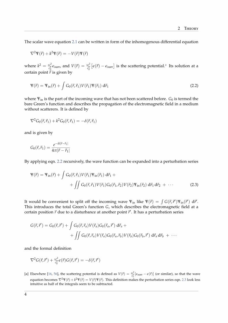
The scalar wave equation 2.1 can be written in form of the inhomogenous differential equation
∇2Ψ(~r) + k2Ψ(~r) = −V(~r)Ψ(~r)
where k2 = ω2
c20
εsurr, and V(~r) = ω2
c20
[ε(~r)− εsurr
]is the scattering potential.a Its solution at a
certain point~r is given by
Ψ(~r) = Ψin(~r) +∫
G0(~r,~r1)V(~r1)Ψ(~r1) d~r1 (2.2)
where Ψin is the part of the incoming wave that has not been scattered before. G0 is termed thebare Green’s function and describes the propagation of the electromagnetic field in a mediumwithout scatterers. It is defined by
∇2G0(~r,~r1) + k2G0(~r,~r1) = −δ(~r,~r1)
and is given by
G0(~r,~r1) =e−ik|~r−~r1|
4π|~r−~r1|
By applying eqn. 2.2 recursively, the wave function can be expanded into a perturbation series
Ψ(~r) = Ψin(~r) +∫
G0(~r,~r1)V(~r1)Ψin(~r1) d~r1 +
+∫∫
G0(~r,~r1)V(~r1)G0(~r1,~r2)V(~r2)Ψin(~r2) d~r1 d~r2 + · · · (2.3)
It would be convenient to split off the incoming wave Ψin like Ψ(~r) =∫
G(~r,~r′)Ψin(~r′) d~r′.This introduces the total Green’s function G, which describes the electromagnetic field at acertain position~r due to a disturbance at another point~r′. It has a perturbation series
G(~r,~r′) = G0(~r,~r′) +∫
G0(~r,~ra)V(~ra)G0(~ra,~r′) d~ra +
+∫∫
G0(~r,~ra)V(~ra)G0(~ra,~rb)V(~rb)G0(~rb,~r′) d~ra d~rb + · · ·
and the formal definition
∇2G(~r,~r′) + ω2
c20
ε(~r)G(~r,~r′) = −δ(~r,~r′)
[a] Elsewhere [16, 56], the scattering potential is defined as V(~r) = ω2
c20[εsurr − ε(~r)] (or similar), so that the wave
equation becomes ∇2Ψ(~r) + k2Ψ(~r) = V(~r)Ψ(~r). This definition makes the perturbation series eqn. 2.3 look lessintuitive as half of the integrals seem to be subtracted.
4
2.2 Single scattering – Mie theory
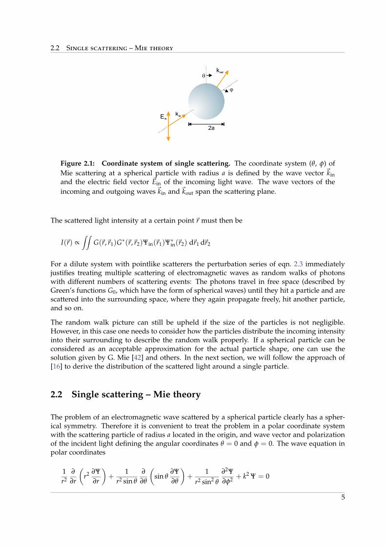
Figure 2.1: Coordinate system of single scattering. The coordinate system (θ, φ) ofMie scattering at a spherical particle with radius a is defined by the wave vector ~kinand the electric field vector ~Ein of the incoming light wave. The wave vectors of theincoming and outgoing waves~kin and~kout span the scattering plane.
The scattered light intensity at a certain point~r must then be
I(~r) ∝∫∫
G(~r,~r1)G∗(~r,~r2)Ψin(~r1)Ψ∗in(~r2) d~r1 d~r2
For a dilute system with pointlike scatterers the perturbation series of eqn. 2.3 immediatelyjustifies treating multiple scattering of electromagnetic waves as random walks of photonswith different numbers of scattering events: The photons travel in free space (described byGreen’s functions G0, which have the form of spherical waves) until they hit a particle and arescattered into the surrounding space, where they again propagate freely, hit another particle,and so on.
The random walk picture can still be upheld if the size of the particles is not negligible.However, in this case one needs to consider how the particles distribute the incoming intensityinto their surrounding to describe the random walk properly. If a spherical particle can beconsidered as an acceptable approximation for the actual particle shape, one can use thesolution given by G. Mie [42] and others. In the next section, we will follow the approach of[16] to derive the distribution of the scattered light around a single particle.
2.2 Single scattering – Mie theory
The problem of an electromagnetic wave scattered by a spherical particle clearly has a spher-ical symmetry. Therefore it is convenient to treat the problem in a polar coordinate systemwith the scattering particle of radius a located in the origin, and wave vector and polarizationof the incident light defining the angular coordinates θ = 0 and φ = 0. The wave equation inpolar coordinates
1r2
∂
∂r
(r2 ∂Ψ
∂r
)+
1r2 sin θ
∂
∂θ
(sin θ
∂Ψ∂θ
)+
1r2 sin2 θ
∂2Ψ∂φ2 + k2 Ψ = 0
5
2 Theory
can be separated into three independent differential equations using the ansatz Ψ(r, θ, φ) =R(r) ·Θ(θ) ·Φ(φ):
1R
ddr
(r2 dR
dr
)+ k2r2 = α
sin θ
Θddθ
(sin θ
dΘdθ
)= β− α sin2 θ
1Φ
d2Φdφ2 = −β
Setting β = m2 and α = n(n + 1) where m = 0, 1, 2, . . . and n = m, m + 1, . . . we obtain thecomplete solution Ψ for the wave equation, and from this the vector harmonics ~M = ~∇× (~rΨ)
and ~N =~∇× ~M
k .
The solution of the radial part of the wave equation R(r) is given by a linear combination ofthe spherical Bessel functions jn(ρ) =
√π2ρ Jn+1/2(ρ) and yn =
√π2ρ Yn+1/2(ρ) where Jν(ρ) and
Yν(ρ) are Bessel functions of first and second kind, and ρ = kr. For the outgoing scatteredwave the appropriate linear combination is given by one of the spherical Bessel functions ofthe third kind or spherical Hankel functions, h(1)n (ρ) = jn(ρ) + iyn(ρ).
The zenith part of the wave equation Θ(θ) is solved by associated Legendre functions Pmn (cos θ).
For the following calculations it is convenient to define the angle-dependent functions πn =P1
nsin θ and τn = dP1
ndθ .
It can be shown that the solution for the scattered electric field is given by
~Escat =∞
∑n=1
inE02n + 1
n(n + 1)
(ian~Nn − bn ~Mn
)
where the applicable vector harmonics are given by
~Mn = cos φ πn(cos θ) h(1)n (ρ) eθ − sin φ τn(cos θ) h(1)n (ρ) eφ
~Nn = cos φ n(n + 1) sin θ πn(cos θ)h(1)n (ρ)
ρer + cos φ τn(cos θ)
[ρh(1)n (ρ)]′
ρeθ −
− sin φ πn(cos θ)[ρh(1)n (ρ)]′
ρeφ
and the coefficients an and bn are
an =m ψn(mx) ψ′n(x)− ψn(x) ψ′n(mx)m ψn(mx) ξ ′n(x)− ξn(x) ψ′n(mx)
; bn =ψn(mx) ψ′n(x)−m ψn(x) ψ′n(mx)ψn(mx) ξ ′n(x)−m ξn(x) ψ′n(mx)
6
2.2 Single scattering – Mie theory
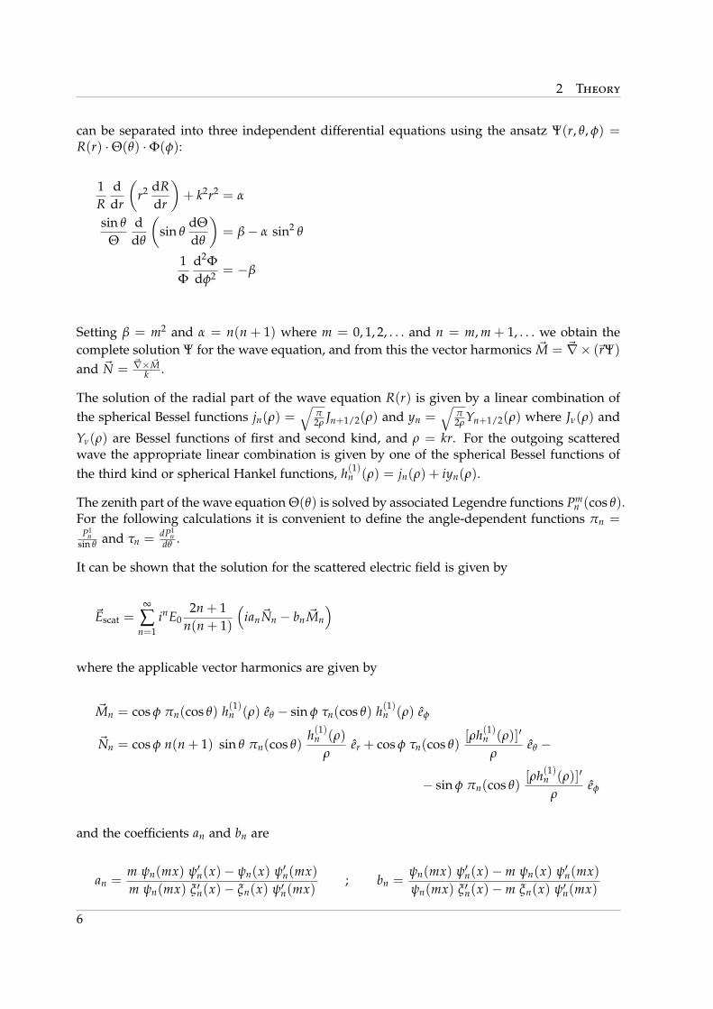
Figure 2.2: Vibration ellipse. The tip of the electric field vector of a light wave tracesout an ellipse with semimajor axis r1, semiminor axis r2, azimuth γ, and ellipticityη = arctan(r2/r1).
with the size parameter x = ka, the relative refractive index m = kscatk , and the Riccati-Bessel
functions ψn(z) = z jn(z) and ξn(z) = z h(1)n (z). The prime indicates differentiation withrespect to the argument in parentheses.
~M has no radial component, and in the far-field limit with large ρ = kr the radial componentof ~N is negligible compared to the transverse component, as the spherical Hankel function is
asymptotically given by h(1)n (kr) ≈ − (−i)neikr
ikr . The scattered electromagnetic field is thereforebasically transverse, and
Eθ ≈ E0 ·eikr
−ikr· cos φ · S2(cos θ) with S2 =
nc
∑n=1
2n + 1n(n + 1)
(anτn + bnπn)
Eφ ≈ −E0 ·eikr
−ikr· sin φ · S1(cos θ) with S1 =
nc
∑n=1
2n + 1n(n + 1)
(anπn + bnτn)
Both sums converge, so that the series can be terminated after nc steps without causing majorinaccuracies. A good assumption is nc ≈ x.
We now focus on a certain scattering plane, which is defined by the wave vectors of theincoming and emerging waves. Intensity and polarization of the scattered light are thenmerely a function of the scattering angle θ and the polarization of the incoming light withrespect to the scattering plane.
In a non-absorbing medium, both incoming and scattered electromagnetic waves can be char-acterized by a Stokes vector [30]
~p =
IQUV
=
1
cos(2η) cos(2γ)cos(2η) sin(2γ)
sin(2η)
7
2 Theory
−180 −135 −90 −45 0 45 90 135 180−45
−30
−15
0
15
30
45
scattering angle [deg]
ellip
ticity
/ az
imut
h [d
eg]
azimuth ellipticity
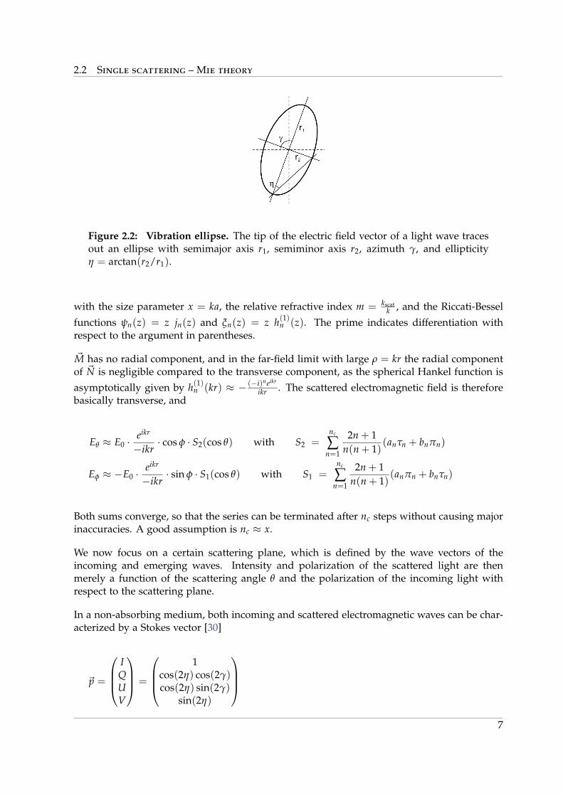
Figure 2.3: Polarization of a scattered wave. The polarization of the scattered wave –which can be described by azimuthal angle γ and ellipticity η – fluctuates strongly asa function of the scattering angle theta. The example shows the scattering of a linearlypolarized wave with wavelength λ = 575 nm and azimuth γ = 45 on a sphericalparticle with diameter 2a = 300 nm and refractive index n = 2.7.
The ellipticity of the vibration ellipse (fig. 2.2) is then given by | tan(2η)| = UQ , the azimuthal
angle by tan(2γ) = V√Q2+U2
.
The transformation between the Stokes vectors of the incident and the scattered light waves isdescribed by so-called Mueller matrices [43]. The Mueller matrix of a spherical particle is
S(cos θ) =1
k2r2
S11 S12 0 0S21 S22 0 00 0 S33 S340 0 S43 S44
where
S11 = S22 = 12 (S2S∗2 + S1S∗1)
S12 = S21 = 12 (S2S∗2 − S1S∗1)
S33 = S44 = 12 (S
∗2S1 + S2S∗1)
S34 = −S43 = i2 (S
∗2S1 − S2S∗1)
As shown by the example in figs. 2.3 and 2.4, in the Mie scattering regime with wavelengthλ ≈ a the polarization of the scattered light and the scattered intensity itself are very unevenlydistributed around the scattering particle. Generally, one can recognize a transition from theisotropic intensity distribution of Raleigh scattering in the regime λ a to a significantlyenhanced scattering in forward direction in the Mie regime.
The total scattering cross section
Cscat =2π
k2
∞
∑n=1
(2n + 1)(|an|2 + |bn|2
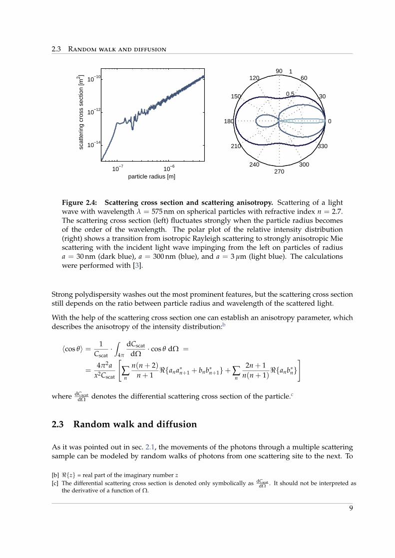
)which is a measure of the scattering efficiency, also fluctuates strongly when the particlediameter becomes of the order of the wavelength (fig. 2.4). For nearly monodisperse scatterersthese so-called Mie resonances can be used to create especially strongly scattering samples.
8
2.3 Random walk and diffusion
10−7
10−6
10−14
10−12
10−10
particle radius [m]
scat
terin
g cr
oss
sect
ion
[m2 ]
0.5
1
30
210
60
240
90
270
120
300
150
330
180 0
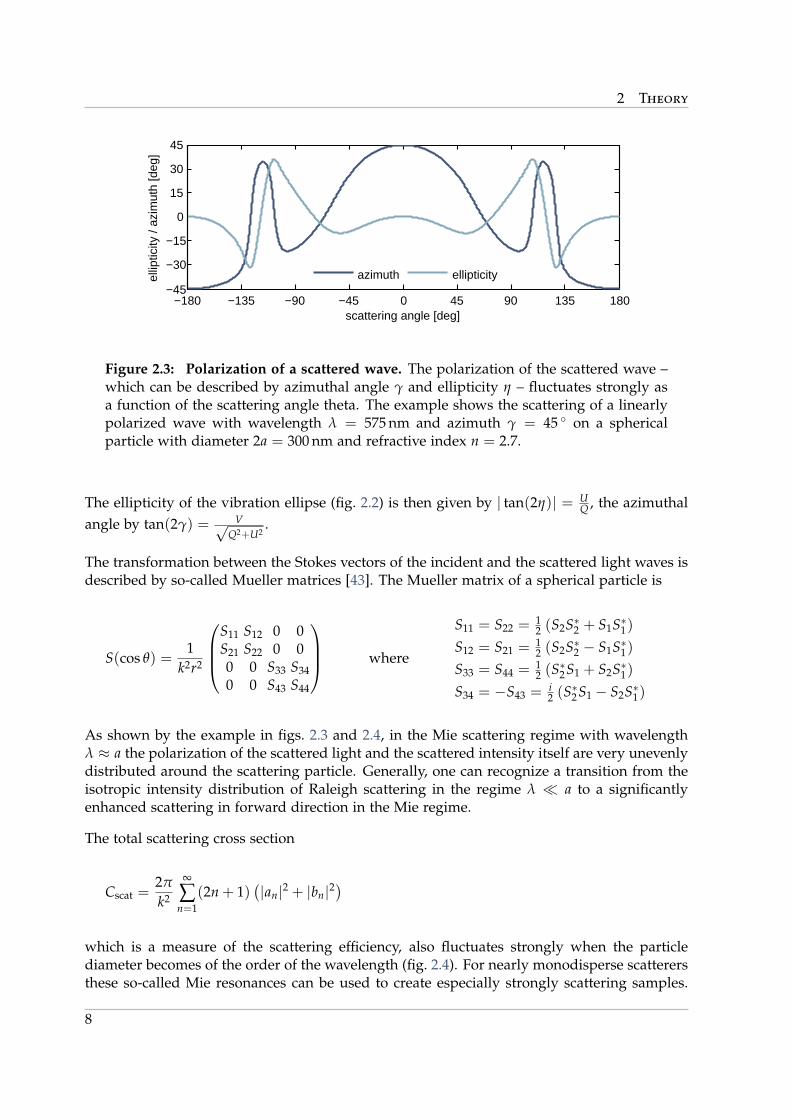
Figure 2.4: Scattering cross section and scattering anisotropy. Scattering of a lightwave with wavelength λ = 575 nm on spherical particles with refractive index n = 2.7.The scattering cross section (left) fluctuates strongly when the particle radius becomesof the order of the wavelength. The polar plot of the relative intensity distribution(right) shows a transition from isotropic Rayleigh scattering to strongly anisotropic Miescattering with the incident light wave impinging from the left on particles of radiusa = 30 nm (dark blue), a = 300 nm (blue), and a = 3 µm (light blue). The calculationswere performed with [3].
Strong polydispersity washes out the most prominent features, but the scattering cross sectionstill depends on the ratio between particle radius and wavelength of the scattered light.
With the help of the scattering cross section one can establish an anisotropy parameter, whichdescribes the anisotropy of the intensity distribution:b
〈cos θ〉 = 1Cscat
·∫
4π
dCscat
dΩ· cos θ dΩ =
=4π2a
x2Cscat
[∑n
n(n + 2)n + 1
<ana∗n+1 + bnb∗n+1+ ∑n
2n + 1n(n + 1)
<anb∗n]
where dCscatdΩ denotes the differential scattering cross section of the particle.c
2.3 Random walk and diffusion
As it was pointed out in sec. 2.1, the movements of the photons through a multiple scatteringsample can be modeled by random walks of photons from one scattering site to the next. To
[b] <z = real part of the imaginary number z[c] The differential scattering cross section is denoted only symbolically as dCscat
dΩ . It should not be interpreted asthe derivative of a function of Ω.
9
2 Theory
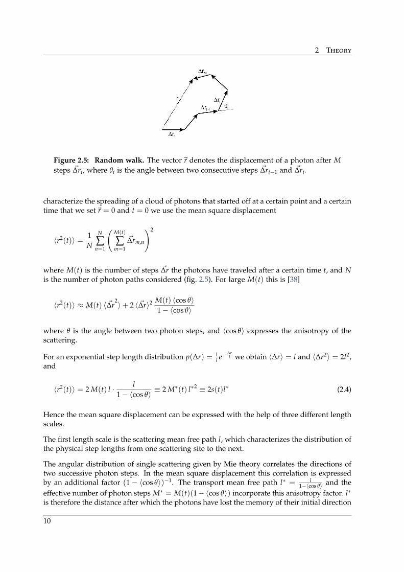
Figure 2.5: Random walk. The vector~r denotes the displacement of a photon after Msteps ~∆ri, where θi is the angle between two consecutive steps ~∆ri−1 and ~∆ri.
characterize the spreading of a cloud of photons that started off at a certain point and a certaintime that we set~r = 0 and t = 0 we use the mean square displacement
〈r2(t)〉 = 1N
N
∑n=1
(M(t)
∑m=1
~∆rm,n
)2
where M(t) is the number of steps ~∆r the photons have traveled after a certain time t, and Nis the number of photon paths considered (fig. 2.5). For large M(t) this is [38]
〈r2(t)〉 ≈ M(t) 〈~∆r2〉+ 2 〈~∆r〉2 M(t) 〈cos θ〉
1− 〈cos θ〉
where θ is the angle between two photon steps, and 〈cos θ〉 expresses the anisotropy of thescattering.
For an exponential step length distribution p(∆r) = 1l e−
∆rl we obtain 〈∆r〉 = l and 〈∆r2〉 = 2l2,
and
〈r2(t)〉 = 2 M(t) l · l1− 〈cos θ〉 ≡ 2 M∗(t) l∗2 ≡ 2s(t)l∗ (2.4)
Hence the mean square displacement can be expressed with the help of three different lengthscales.
The first length scale is the scattering mean free path l, which characterizes the distribution ofthe physical step lengths from one scattering site to the next.
The angular distribution of single scattering given by Mie theory correlates the directions oftwo successive photon steps. In the mean square displacement this correlation is expressedby an additional factor (1− 〈cos θ〉)−1. The transport mean free path l∗ = l
1−〈cos θ〉 and theeffective number of photon steps M∗ = M(t)(1− 〈cos θ〉) incorporate this anisotropy factor. l∗
is therefore the distance after which the photons have lost the memory of their initial direction
10
2.3 Random walk and diffusion
of propagation. The difference between transport mean free path and scattering mean freepath is the larger the more anisotropic the scattering is. For completely isotropic scatteringboth mean free paths are equal.
The product M∗l∗ gives the length s of the photon paths that contribute to the mean squaredisplacement. As there is no reason to assume that the speed of the photons will changealong their path, the length of a photon path is proportional to time. The size of the photoncloud 〈r2(t)〉 at a certain time is therefore linearly proportional to both the length s of thecontributing photon paths and the time t the photons have spent traveling along these paths.
On top of everything, the mean square displacement of eqn. 2.4 is structurally equivalent tothe variance
〈r2(t)〉 = 6Dt (2.5)
of a gaussian distribution in three dimensions
ρ(~r, t) =1
√4πDt
3 e−r2
4Dt (2.6)
where ρ is the density distribution of photons that started off at the origin of the coordinatesystem at time t = 0 in an infinitely extended medium, and D is the diffusion coefficient. Soobviously multiple scattering in the limit of large M(t) can also be described as diffusion oflight energy through the medium with the diffusion equation ∂ρ
∂t − D∇2ρ = δ(t)δ(~r), whosesolution is given by eqn. 2.6
Comparing eqns. 2.4 and 2.5 one can give the diffusion coefficient as
D =sl∗
3t=
vl∗
3(2.7)
where v is the velocity of energy transport. Using this, the photon density distribution canalso be given as a function of the path length s:
ρ(~r, s) =
√3
4πsl∗
3
e− r2
43 sl∗ (2.8)
However, the photon density distribution in a multiply scattering sample is not purely deter-mined by the scattering properties of the scattering particles, but also by energy losses due toabsorption in the material. According to Lambert-Beer’s law, absorption weakens the inten-sity of a light wave exponentially along the traveled path, so that its effect can be includedin the photon density distribution by an additional factor e−
sla or e−
tτ , respectively. The ab-
sorption length la and the absorption time τ are inversely proportional to the number densityρabs of absorbing particles on the path and their absorption cross section σabs: la =
1ρabs σabs
and
τ = ts la =
1v ρabs σabs
.
11
2 Theory
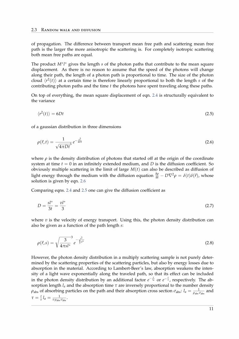
Figure 2.6: Scattering in the presence of a single boundary. All photon paths A→ Bthat are lost because they run partially outside the samples can be described by theirimage paths A → B′. The (virtual) scatterer P is the point where a photon path leavesthe sample.
2.4 The influence of boundaries
Eqns. 2.6 and 2.8 describe the photon density distribution in infinitely extended samples. Inreality however, this distribution is strongly influenced by the borders of the system, wherephotons are inserted and released, absorbed and reflected.
There are two different approaches to describe the influence of boundaries on a multiplescattering system. The more intuitive one is the image point method, which uses symmetryproperties of the density distribution to describe the scattering in terms of the density distribu-tion in infinite space [38]. The other approach is in the framework of radiative transfer theory,which describes a field of radiation by the intensity flux through area elements. This makesit possible to compare the flux through an area element at the sample surface with an areaelement inside the sample and derive theoretical descriptions for the various experimentalsituations [58].
2.4.1 Image point method
To describe multiple scattering in a finite sample in terms of scattering in infinite space onecan make use of the symmetry properties of the density distribution: The photon density atany point B in an infinite sample is equal to the density at its image point B′ with respectto any mirror plane that contains the starting point P of the photon cloud. Therefore we candescribe photon paths A → P → B by paths A → P → B′ that end at the image point of Bwith respect to P. If P is the endpoint of a photon step that leads the path out of the sample,the path A → P → B is not possible in the presence of the boundary, and its contribution ismissing from the free space photon density in B.
12
2.4 The influence of boundaries
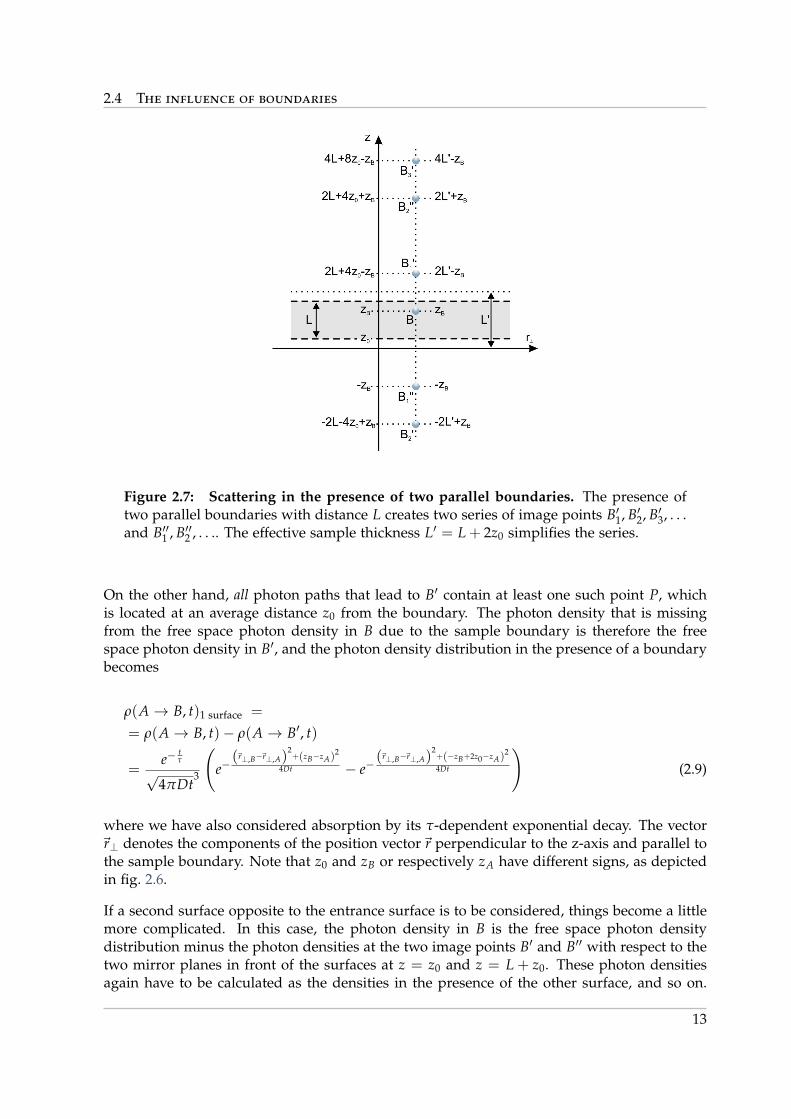
Figure 2.7: Scattering in the presence of two parallel boundaries. The presence oftwo parallel boundaries with distance L creates two series of image points B′1, B′2, B′3, . . .and B′′1 , B′′2 , . . .. The effective sample thickness L′ = L + 2z0 simplifies the series.
On the other hand, all photon paths that lead to B′ contain at least one such point P, whichis located at an average distance z0 from the boundary. The photon density that is missingfrom the free space photon density in B due to the sample boundary is therefore the freespace photon density in B′, and the photon density distribution in the presence of a boundarybecomes
ρ(A→ B, t)1 surface =
= ρ(A→ B, t)− ρ(A→ B′, t)
=e−
tτ
√4πDt
3
(e−
(~r⊥,B−~r⊥,A)2+(zB−zA)
2
4Dt − e−(~r⊥,B−~r⊥,A)
2+(−zB+2z0−zA)
2
4Dt
)(2.9)
where we have also considered absorption by its τ-dependent exponential decay. The vector~r⊥ denotes the components of the position vector~r perpendicular to the z-axis and parallel tothe sample boundary. Note that z0 and zB or respectively zA have different signs, as depictedin fig. 2.6.
If a second surface opposite to the entrance surface is to be considered, things become a littlemore complicated. In this case, the photon density in B is the free space photon densitydistribution minus the photon densities at the two image points B′ and B′′ with respect to thetwo mirror planes in front of the surfaces at z = z0 and z = L + z0. These photon densitiesagain have to be calculated as the densities in the presence of the other surface, and so on.
13
2 Theory
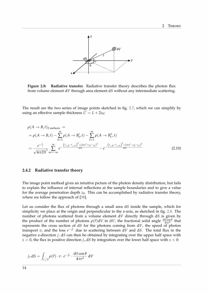
Figure 2.8: Radiative transfer. Radiative transfer theory describes the photon fluxfrom volume element dV through area element dS without any intermediate scattering.
The result are the two series of image points sketched in fig. 2.7, which we can simplify byusing an effective sample thickness L′ = L + 2z0:
ρ(A→ B, t)2 surfaces =
= ρ(A→ B, t)−∞
∑k=1
ρ(A→ B′k, t)−∞
∑k=1
ρ(A→ B′′k , t)
=e−
tτ
√4πDt
3
∞
∑m=−∞
e−(~r⊥,B−~r⊥,A)
2+(2mL′+zB−zA)
2
4Dt − e−(~r⊥,B−~r⊥,A)
2+(2mL′−zB−zA)
2
4Dt (2.10)
2.4.2 Radiative transfer theory
The image point method gives an intuitive picture of the photon density distribution, but failsto explain the influence of internal reflections at the sample boundaries and to give a valuefor the average penetration depth z0. This can be accomplished by radiative transfer theory,where we follow the approach of [58].
Let us consider the flux of photons through a small area dS inside the sample, which forsimplicity we place at the origin and perpendicular to the z-axis, as sketched in fig. 2.8. Thenumber of photons scattered from a volume element dV directly through dS is given bythe product of the number of photons ρ(~r)dV in dV, the fractional solid angle dS cos θ
4πr2 thatrepresents the cross section of dS for the photons coming from dV, the speed of photontransport v, and the loss e−
rl∗ due to scattering between dV and dS. The total flux in the
negative z-direction j−dS can then be obtained by integrating over the upper half space withz > 0, the flux in positive direction j+dS by integration over the lower half space with z < 0:
j∓dS =∫
z >< 0
ρ(~r) · v · e− rl∗ · dS cos θ
4πr2 dV
14
2.5 Photon flux from a surface
The main contribution of the flux comes from the immediate neighborhood of dS, so thatthe photon density can be replaced by its first-order Taylor expansion around the origin.Evaluation of the integral then yields
j∓ =ρ0v4± vl∗
6
(∂ρ
∂z
)0
where the photon density and its derivative have to be taken at the origin.
If dS is located at a boundary, there will be no flux from outside the sample, but internalreflections will create an apparent flux from this direction, which is related to the outgoingflux by the reflectivity R of the surface: jin = R · jout. This gives the boundary conditions
ρ− 2l∗
31 + R1− R
· ∂ρ
∂z= 0 for an upper boundary, i.e. j+ = R · j− and
ρ +2l∗
31 + R1− R
· ∂ρ
∂z= 0 for a lower boundary, i.e. j− = R · j+
The point where the photon density drops to zero is not located at the boundary but at adistance 2l∗
31+R1−R ·
∂ρ∂z in front of it. We can identify this distance with the average penetration
depth z0 which we have used above for the image point method, as this also is the point wherethe photon density vanishes. Assuming a constant gradient of the photon density distributionclose to the surface, one obtains |z0| = 2l∗
31+R1−R ≈ 0.67 1+R
1−R l∗. Other solutions are mostly of theorder of |z0| ≈ 0.7 for the limit of non-reflective surfaces (see e.g. [53], [54]).
2.5 Photon flux from a surface
The experimentally accessible quantity in multiple scattering experiments is not the photondensity distribution inside the sample, but the light intensity emitted from a sample surface.It is obvious that this intensity (or photon flux density) is proportional to the number ofphotons, i.e. the photon density, at the surface. One can therefore easily calculate the expectedintensities for the various experimental situations from eqns. 2.9 and 2.10.
2.5.1 Backscattering geometry
Backscattering experiments are usually performed with thick samples, where the influence ofthe rear and side surfaces on the photon density distribution can be neglected, and the sampleis well described as an infinite half-space.
In backscattering geometry, photon paths of all lengths contribute to the intensity at the sur-face, so that the latter is not fully described by the solution of the diffusion equation, which isvalid only for long photon paths. It has been shown however [44] that correct results can be
15
2 Theory
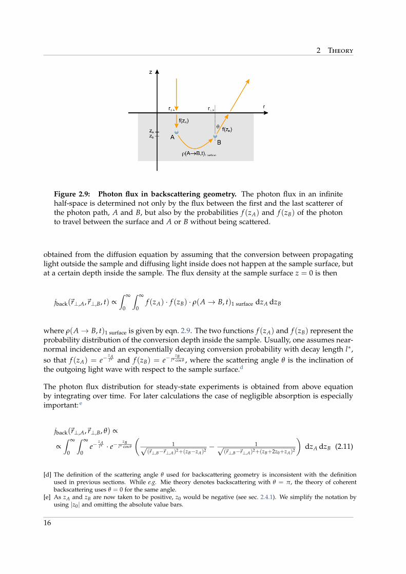
Figure 2.9: Photon flux in backscattering geometry. The photon flux in an infinitehalf-space is determined not only by the flux between the first and the last scatterer ofthe photon path, A and B, but also by the probabilities f (zA) and f (zB) of the photonto travel between the surface and A or B without being scattered.
obtained from the diffusion equation by assuming that the conversion between propagatinglight outside the sample and diffusing light inside does not happen at the sample surface, butat a certain depth inside the sample. The flux density at the sample surface z = 0 is then
jback(~r⊥,A,~r⊥,B, t) ∝∫ ∞
0
∫ ∞
0f (zA) · f (zB) · ρ(A→ B, t)1 surface dzA dzB
where ρ(A→ B, t)1 surface is given by eqn. 2.9. The two functions f (zA) and f (zB) represent theprobability distribution of the conversion depth inside the sample. Usually, one assumes near-normal incidence and an exponentially decaying conversion probability with decay length l∗,so that f (zA) = e−
zAl∗ and f (zB) = e−
zBl∗ cos θ , where the scattering angle θ is the inclination of
the outgoing light wave with respect to the sample surface.d
The photon flux distribution for steady-state experiments is obtained from above equationby integrating over time. For later calculations the case of negligible absorption is especiallyimportant: e
jback(~r⊥,A,~r⊥,B, θ) ∝
∝∫ ∞
0
∫ ∞
0e−
zAl∗ · e−
zBl∗ cos θ
(1√
(~r⊥,B−~r⊥,A)2+(zB−zA)2− 1√
(~r⊥,B−~r⊥,A)2+(zB+2z0+zA)2
)dzA dzB (2.11)
[d] The definition of the scattering angle θ used for backscattering geometry is inconsistent with the definitionused in previous sections. While e.g. Mie theory denotes backscattering with θ = π, the theory of coherentbackscattering uses θ = 0 for the same angle.
[e] As zA and zB are now taken to be positive, z0 would be negative (see sec. 2.4.1). We simplify the notation byusing |z0| and omitting the absolute value bars.
16
2.6 On polarization and interference
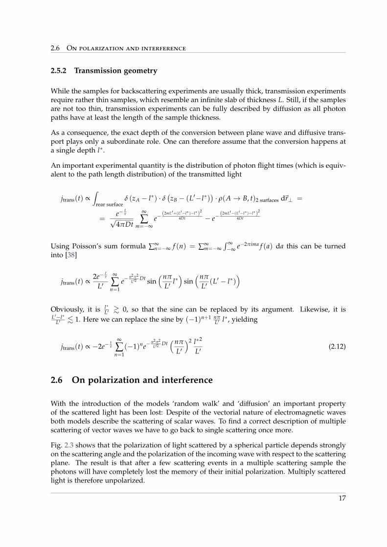
2.5.2 Transmission geometry
While the samples for backscattering experiments are usually thick, transmission experimentsrequire rather thin samples, which resemble an infinite slab of thickness L. Still, if the samplesare not too thin, transmission experiments can be fully described by diffusion as all photonpaths have at least the length of the sample thickness.
As a consequence, the exact depth of the conversion between plane wave and diffusive trans-port plays only a subordinate role. One can therefore assume that the conversion happens ata single depth l∗.
An important experimental quantity is the distribution of photon flight times (which is equiv-alent to the path length distribution) of the transmitted light
jtrans(t) ∝∫
rear surfaceδ (zA − l∗) · δ
(zB − (L′−l∗)
)· ρ(A→ B, t)2 surfaces d~r⊥ =
=e−
tτ
√4πDt
∞
∑m=−∞
e−(2mL′+(L′−l∗)−l∗)2
4Dt − e−(2mL′−(L′−l∗)−l∗)2
4Dt
Using Poisson’s sum formula ∑∞n=−∞ f (n) = ∑∞
m=−∞∫ ∞−∞ e−2πima f (a) da this can be turned
into [38]
jtrans(t) ∝2e−
tτ
L′∞
∑n=1
e−n2π2
L′2Dt sin
(nπ
L′l∗)
sin(nπ
L′(L′ − l∗)
)
Obviously, it is l∗L′ & 0, so that the sine can be replaced by its argument. Likewise, it is
L′−l∗L′ . 1. Here we can replace the sine by (−1)n+1 nπ
L′ l∗, yielding
jtrans(t) ∝ −2e−tτ
∞
∑n=1
(−1)ne−n2π2
L′2Dt(nπ
L′)2 l∗2
L′(2.12)
2.6 On polarization and interference
With the introduction of the models ‘random walk’ and ‘diffusion’ an important propertyof the scattered light has been lost: Despite of the vectorial nature of electromagnetic wavesboth models describe the scattering of scalar waves. To find a correct description of multiplescattering of vector waves we have to go back to single scattering once more.
Fig. 2.3 shows that the polarization of light scattered by a spherical particle depends stronglyon the scattering angle and the polarization of the incoming wave with respect to the scatteringplane. The result is that after a few scattering events in a multiple scattering sample thephotons will have completely lost the memory of their initial polarization. Multiply scatteredlight is therefore unpolarized.
17
2 Theory
100 200 300
50
100
150
200
250
300
1
2
3
4
5
x 104
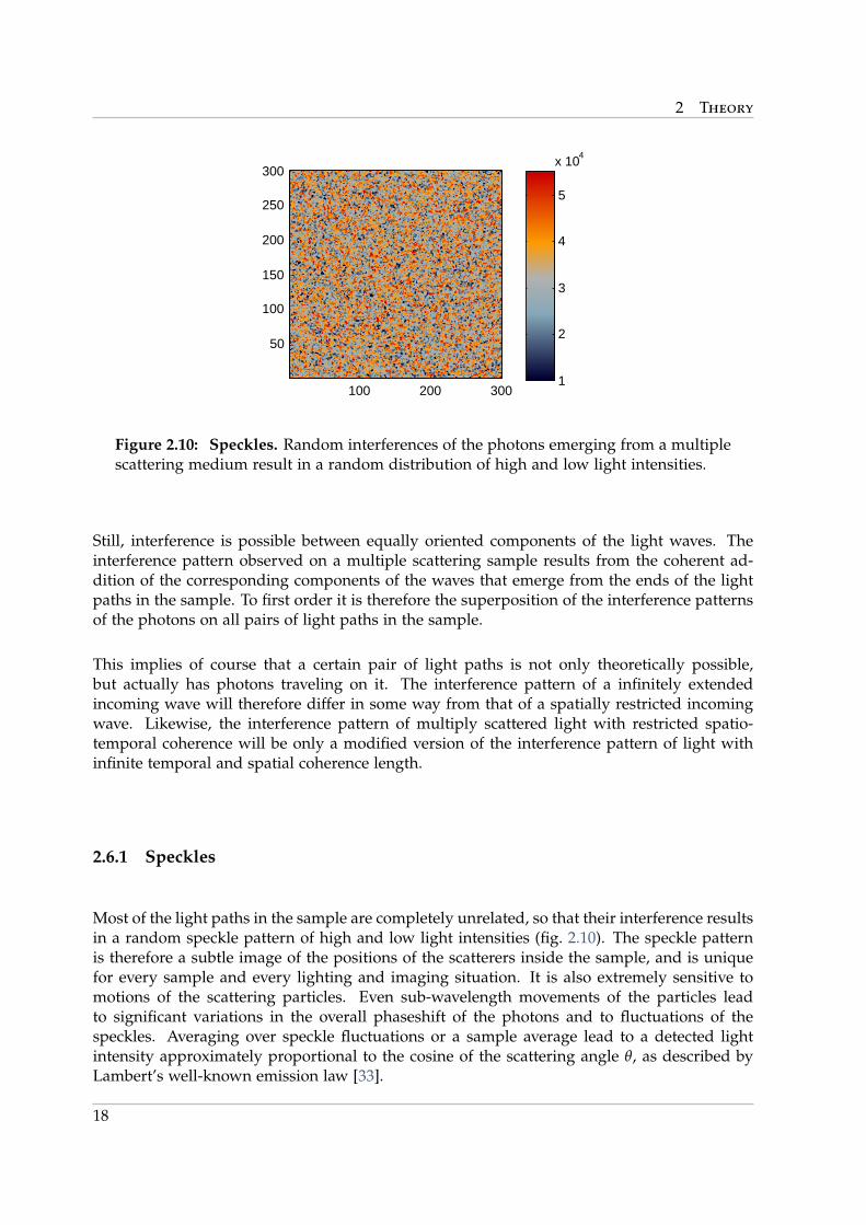
Figure 2.10: Speckles. Random interferences of the photons emerging from a multiplescattering medium result in a random distribution of high and low light intensities.
Still, interference is possible between equally oriented components of the light waves. Theinterference pattern observed on a multiple scattering sample results from the coherent ad-dition of the corresponding components of the waves that emerge from the ends of the lightpaths in the sample. To first order it is therefore the superposition of the interference patternsof the photons on all pairs of light paths in the sample.
This implies of course that a certain pair of light paths is not only theoretically possible,but actually has photons traveling on it. The interference pattern of a infinitely extendedincoming wave will therefore differ in some way from that of a spatially restricted incomingwave. Likewise, the interference pattern of multiply scattered light with restricted spatio-temporal coherence will be only a modified version of the interference pattern of light withinfinite temporal and spatial coherence length.
2.6.1 Speckles
Most of the light paths in the sample are completely unrelated, so that their interference resultsin a random speckle pattern of high and low light intensities (fig. 2.10). The speckle patternis therefore a subtle image of the positions of the scatterers inside the sample, and is uniquefor every sample and every lighting and imaging situation. It is also extremely sensitive tomotions of the scattering particles. Even sub-wavelength movements of the particles leadto significant variations in the overall phaseshift of the photons and to fluctuations of thespeckles. Averaging over speckle fluctuations or a sample average lead to a detected lightintensity approximately proportional to the cosine of the scattering angle θ, as described byLambert’s well-known emission law [33].
18
2.6 On polarization and interference
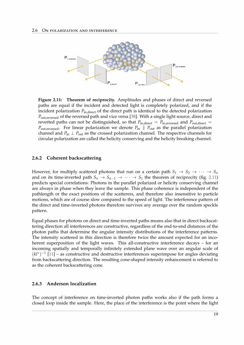
Figure 2.11: Theorem of reciprocity. Amplitudes and phases of direct and reversedpaths are equal if the incident and detected light is completely polarized, and if theincident polarization Pin,direct of the direct path is identical to the detected polarizationPout,reversed of the reversed path and vice versa [38]. With a single light source, direct andreverted paths can not be distinguished, so that Pin,direct = Pin,reversed and Pout,direct =Pout,reversed. For linear polarization we denote Pin ‖ Pout as the parallel polarizationchannel and Pin ⊥ Pout as the crossed polarization channel. The respective channels forcircular polarization are called the helicity conserving and the helicity breaking channel.
2.6.2 Coherent backscattering
However, for multiply scattered photons that run on a certain path S1 → S2 → · · · → Snand on its time-inverted path Sn → Sn−1 → · · · → S1 the theorem of reciprocity (fig. 2.11)predicts special correlations: Photons in the parallel polarized or helicity conserving channelare always in phase when they leave the sample. This phase coherence is independent of thepathlength or the exact positions of the scatterers, and therefore also insensitive to particlemotions, which are of course slow compared to the speed of light. The interference pattern ofthe direct and time-inverted photons therefore survives any average over the random specklepattern.
Equal phases for photons on direct and time-inverted paths means also that in direct backscat-tering direction all interferences are constructive, regardless of the end-to-end distances of thephoton paths that determine the angular intensity distributions of the interference patterns.The intensity scattered in this direction is therefore twice the amount expected for an inco-herent superposition of the light waves. This all-constructive interference decays – for anincoming spatially and temporally infinitely extended plane wave over an angular scale of(kl∗)−1 [11] – as constructive and destructive interferences superimpose for angles deviatingfrom backscattering direction. The resulting cone-shaped intensity enhancement is referred toas the coherent backscattering cone.
2.6.3 Anderson localization
The concept of interference on time-inverted photon paths works also if the path forms aclosed loop inside the sample. Here, the place of the interference is the point where the light
19

2 Theory
waves enter and leave the loop. As the light waves are always in phase at this point, con-structive interference leads to an enhanced photon density compared to the normal diffusivebehavior. In strongly scattering media the probability of photons running on closed loops isenhanced, so that a macroscopically reduced diffusion can be observed. Eventually this leadsto a complete breakdown of photon transport and a transition to a localizing state, which iscalled Anderson localization [13].
The critical amount of disorder for this phase transition can be expressed by the criterionproposed by Ioffe and Regel [27], namely that kl∗ ≈ 1. The width of the steady-state coherentbackscattering cone, which is inversely proportional to this quantity, is therefore an importantexperimental measure for the disorder in the sample [12].
2.7 The theory of coherent backscattering
To develop a theory for the steady-state coherent backscattering cone, the easiest case to con-sider is a uniform plane wave with infinite spatio-temporal coherence impinging perpendicu-larly on the surface of a non-absorbing multiple scattering medium. In this case the photonflux distribution has the simple form given in eqn. 2.11, and furthermore is translationallyinvariant, i.e. jback(~r⊥,A,~r⊥,B, θ) becomes jback(~r⊥, θ) with~r⊥ =~r⊥,B −~r⊥,A.
We define the cooperon αc(θ) as the coherent and the diffuson αd(θ) as the incoherent additionof the flux emerging from the time-inverted paths in the sample:
αd(θ) =
∫jback(~r⊥, θ) d~r⊥∫
jback(~r⊥, θ = 0) d~r⊥and αc(θ) =
∫jback(~r⊥, θ) · ei~k~r⊥ d~r⊥∫jback(~r⊥, θ = 0) d~r⊥
(2.13)
where~k is the wave vector of the emitted light wave. The diffuson is sometimes also referredto as the incoherent background of the backscattering cone.
If single and low order scattering can be blocked completely, the backscattered intensity mea-sured in an experiment is the sum of these two contributions. Otherwise, the height of thecooperon compared to the diffuson is reduced, as single scattering contributes to the incoher-ent, but not to the coherent addition of the photon flux [38].
Evaluating the above equations yields [10]
αd(θ) =µ(
z0l∗ +
µµ+1
)z0l∗ +
12
(2.14)
and
αc(θ) =
1−e−2qz0ql∗ + 2µ
µ+1
2( z0
l∗ +12
) (ql∗ + µ+1
2µ
)2 (2.15)
20
2.7 The theory of coherent backscattering
−90 −60 −30 0 30 60 90
0
0.2
0.4
0.6
0.8
1
1.2
1.4
1.6
1.8
2
scattering angle [deg]
diffu
son
/ coo
pero
n
diffuson α
d(θ)
cooperon αc(θ)
αd(θ) + α
c(θ)
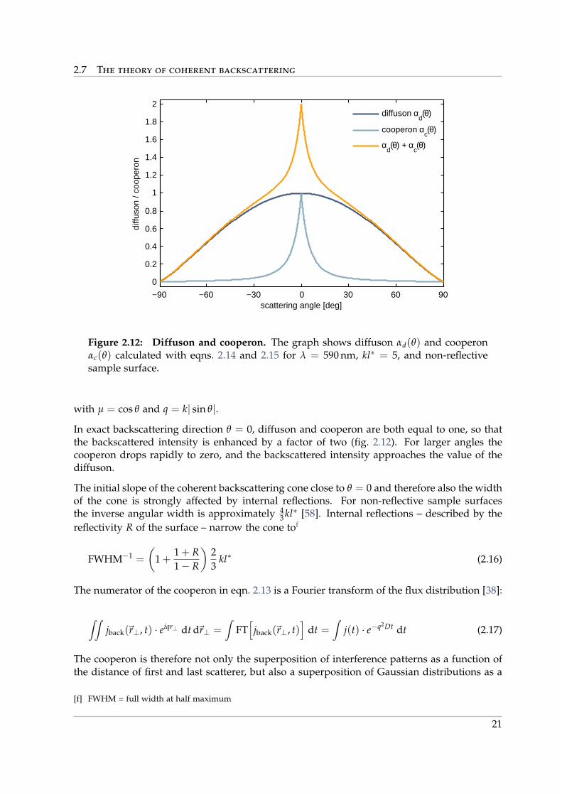
Figure 2.12: Diffuson and cooperon. The graph shows diffuson αd(θ) and cooperonαc(θ) calculated with eqns. 2.14 and 2.15 for λ = 590 nm, kl∗ = 5, and non-reflectivesample surface.
with µ = cos θ and q = k| sin θ|.
In exact backscattering direction θ = 0, diffuson and cooperon are both equal to one, so thatthe backscattered intensity is enhanced by a factor of two (fig. 2.12). For larger angles thecooperon drops rapidly to zero, and the backscattered intensity approaches the value of thediffuson.
The initial slope of the coherent backscattering cone close to θ = 0 and therefore also the widthof the cone is strongly affected by internal reflections. For non-reflective sample surfacesthe inverse angular width is approximately 4
3 kl∗ [58]. Internal reflections – described by thereflectivity R of the surface – narrow the cone tof
FWHM−1 =
(1 +
1 + R1− R
)23
kl∗ (2.16)
The numerator of the cooperon in eqn. 2.13 is a Fourier transform of the flux distribution [38]:
∫∫jback(~r⊥, t) · eiqr⊥ dt d~r⊥ =
∫FT[
jback(~r⊥, t)]
dt =∫
j(t) · e−q2Dt dt (2.17)
The cooperon is therefore not only the superposition of interference patterns as a function ofthe distance of first and last scatterer, but also a superposition of Gaussian distributions as a
[f] FWHM = full width at half maximum
21
2 Theory
−90 −60 −30 0 30 60 90
0
0.2
0.4
0.6
0.8
1
scattering angle [deg]
coop
eron
labs
= 10−5 m
labs
= 3 ⋅ 10−5 m
labs
= 10−4 m
no absorption
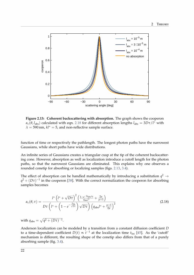
Figure 2.13: Coherent backscattering with absorption. The graph shows the cooperonαc(θ, labs) calculated with eqn. 2.18 for different absorption lengths labs = 3Dτ/l∗ withλ = 590 nm, kl∗ = 5, and non-reflective sample surface.
function of time or respectively the pathlength. The longest photon paths have the narrowestGaussians, while short paths have wide distributions.
An infinite series of Gaussians creates a triangular cusp at the tip of the coherent backscatter-ing cone. However, absorption as well as localization introduce a cutoff length for the photonpaths, so that the narrowest Gaussians are eliminated. This explains why one observes arounded conetip for absorbing or localizing samples (figs. 2.13, 3.4).
The effect of absorption can be handled mathematically by introducing a substitution q2 →q2 + (Dτ)−1 in the cooperon [38]. With the correct normalization the cooperon for absorbingsamples becomes
αc(θ, τ) =l∗(
l∗ +√
Dτ)2 (
1−e−2qabsz0
qabsl∗ + 2µµ+1
)Dτ
(l∗ +
(1− e−
2z0√Dτ
)√Dτ
)(qabsl∗ + µ+1
2µ
)2(2.18)
with qabs =√
q2 + (Dτ)−1.
Anderson localization can be modeled by a transition from a constant diffusion coefficient Dto a time-dependent coefficient D(t) ∝ t−1 at the localization time tloc [45]. As the ‘cutoff’mechanism is different, the resulting shape of the conetip also differs from that of a purelyabsorbing sample (fig. 3.4).
22
2.7 The theory of coherent backscattering
−90 −60 −30 0 30 60 90
0
0.05
0.1
0.15
0.2
0.25
0.3
scattering angle [deg]
coop
eron
[a.u
.]
labs
= 10−5 m
labs
= 3 ⋅ 10−5 m
labs
= 10−4 m
no absorption
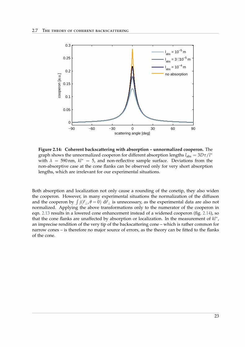
Figure 2.14: Coherent backscattering with absorption – unnormalized cooperon. Thegraph shows the unnormalized cooperon for different absorption lengths labs = 3Dτ/l∗
with λ = 590 nm, kl∗ = 5, and non-reflective sample surface. Deviations from thenon-absorptive case at the cone flanks can be observed only for very short absorptionlengths, which are irrelevant for our experimental situations.
Both absorption and localization not only cause a rounding of the conetip, they also widenthe cooperon. However, in many experimental situations the normalization of the diffusonand the cooperon by
∫j(~r⊥, θ = 0) d~r⊥ is unnecessary, as the experimental data are also not
normalized. Applying the above transformations only to the numerator of the cooperon ineqn. 2.13 results in a lowered cone enhancement instead of a widened cooperon (fig. 2.14), sothat the cone flanks are unaffected by absorption or localization. In the measurement of kl∗,an imprecise rendition of the very tip of the backscattering cone – which is rather common fornarrow cones – is therefore no major source of errors, as the theory can be fitted to the flanksof the cone.
23

2 Theory
24
3 Setups
3.1 Laser System
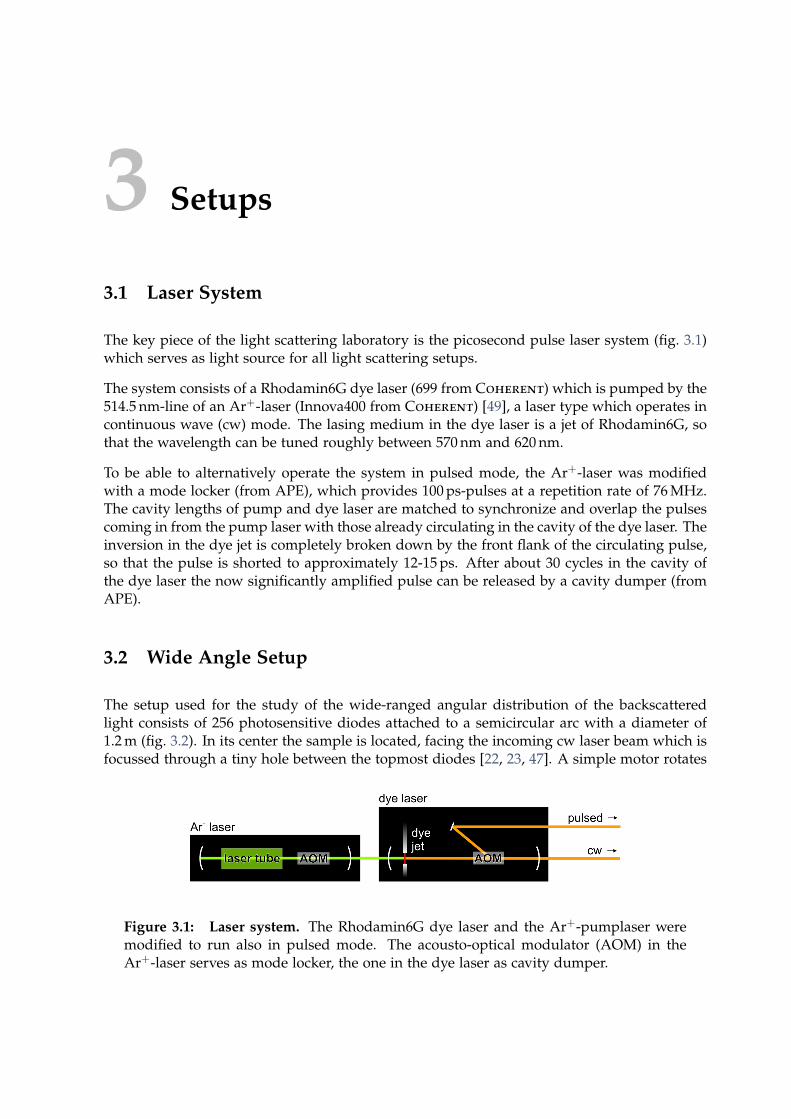
The key piece of the light scattering laboratory is the picosecond pulse laser system (fig. 3.1)which serves as light source for all light scattering setups.
The system consists of a Rhodamin6G dye laser (699 from Coherent) which is pumped by the514.5 nm-line of an Ar+-laser (Innova400 from Coherent) [49], a laser type which operates incontinuous wave (cw) mode. The lasing medium in the dye laser is a jet of Rhodamin6G, sothat the wavelength can be tuned roughly between 570 nm and 620 nm.
To be able to alternatively operate the system in pulsed mode, the Ar+-laser was modifiedwith a mode locker (from APE), which provides 100 ps-pulses at a repetition rate of 76 MHz.The cavity lengths of pump and dye laser are matched to synchronize and overlap the pulsescoming in from the pump laser with those already circulating in the cavity of the dye laser. Theinversion in the dye jet is completely broken down by the front flank of the circulating pulse,so that the pulse is shorted to approximately 12-15 ps. After about 30 cycles in the cavity ofthe dye laser the now significantly amplified pulse can be released by a cavity dumper (fromAPE).
3.2 Wide Angle Setup
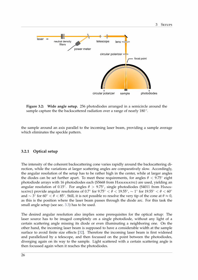
The setup used for the study of the wide-ranged angular distribution of the backscatteredlight consists of 256 photosensitive diodes attached to a semicircular arc with a diameter of1.2 m (fig. 3.2). In its center the sample is located, facing the incoming cw laser beam which isfocussed through a tiny hole between the topmost diodes [22, 23, 47]. A simple motor rotates
Figure 3.1: Laser system. The Rhodamin6G dye laser and the Ar+-pumplaser weremodified to run also in pulsed mode. The acousto-optical modulator (AOM) in theAr+-laser serves as mode locker, the one in the dye laser as cavity dumper.
3 Setups
Figure 3.2: Wide angle setup. 256 photodiodes arranged in a semicircle around thesample capture the the backscattered radiation over a range of nearly 180 .
the sample around an axis parallel to the incoming laser beam, providing a sample averagewhich eliminates the speckle pattern.
3.2.1 Optical setup
The intensity of the coherent backscattering cone varies rapidly around the backscattering di-rection, while the variations at larger scattering angles are comparatively slow. Accordingly,the angular resolution of the setup has to be rather high in the center, while at larger anglesthe diodes can be set further apart. To meet these requirements, for angles θ < 9.75 eightphotodiode arrays with 16 photodiodes each (S5668 from Hamamatsu) are used, yielding anangular resolution of 0.15. For angles θ > 9.75, single photodiodes (S4011 from Hama-matsu) provide angular resolutions of 0.7 for 9.75 < θ < 19.55, ∼ 1 for 19.55 < θ < 60
and ∼ 3 for 60 < θ < 85. Still, it is not possible ro resolve the very tip of the cone at θ ≈ 0,as this is the position where the laser beam passes through the diode arc. For this task thesmall angle setup (see sec. 3.3) has to be used.
The desired angular resolution also implies some prerequisites for the optical setup: Thelaser source has to be imaged completely on a single photodiode, without any light of acertain scattering angle missing its diode or even illuminating a neighboring one. On theother hand, the incoming laser beam is supposed to have a considerable width at the samplesurface to avoid finite size effects [32]. Therefore the incoming laser beam is first widenedand parallelized by a telescope, and then focussed on the point between the photodiodes,diverging again on its way to the sample. Light scattered with a certain scattering angle isthen focussed again when it reaches the photodiodes.
26
3.2 Wide Angle Setup
- 9 0 - 6 0 - 3 0 0 3 0 6 0 9 00 . 0
0 . 2
0 . 4
0 . 6
0 . 8
1 . 0 h e l i c i t y c o n s e r v i n g h e l i c i t y b r e a k i n g
coop
eron
s c a t t e r i n g a n g l e [ d e g ]
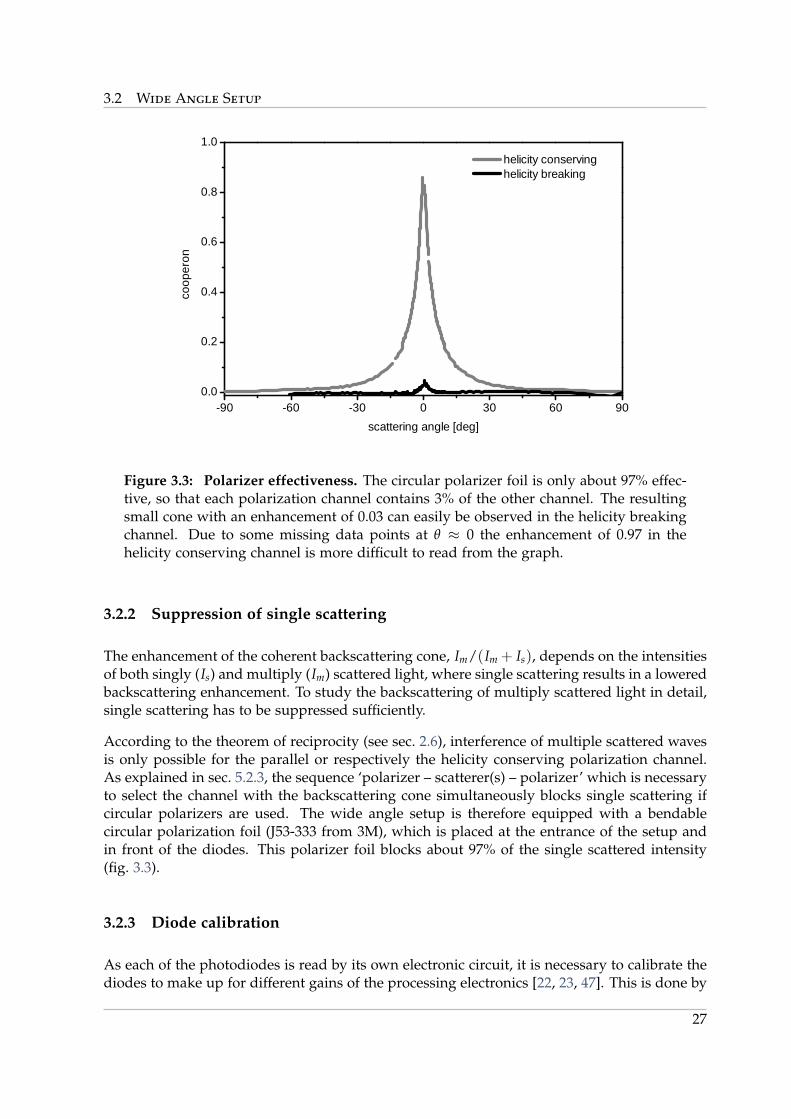
Figure 3.3: Polarizer effectiveness. The circular polarizer foil is only about 97% effec-tive, so that each polarization channel contains 3% of the other channel. The resultingsmall cone with an enhancement of 0.03 can easily be observed in the helicity breakingchannel. Due to some missing data points at θ ≈ 0 the enhancement of 0.97 in thehelicity conserving channel is more difficult to read from the graph.
3.2.2 Suppression of single scattering
The enhancement of the coherent backscattering cone, Im/(Im + Is), depends on the intensitiesof both singly (Is) and multiply (Im) scattered light, where single scattering results in a loweredbackscattering enhancement. To study the backscattering of multiply scattered light in detail,single scattering has to be suppressed sufficiently.
According to the theorem of reciprocity (see sec. 2.6), interference of multiple scattered wavesis only possible for the parallel or respectively the helicity conserving polarization channel.As explained in sec. 5.2.3, the sequence ‘polarizer – scatterer(s) – polarizer’ which is necessaryto select the channel with the backscattering cone simultaneously blocks single scattering ifcircular polarizers are used. The wide angle setup is therefore equipped with a bendablecircular polarization foil (J53-333 from 3M), which is placed at the entrance of the setup andin front of the diodes. This polarizer foil blocks about 97% of the single scattered intensity(fig. 3.3).
3.2.3 Diode calibration
As each of the photodiodes is read by its own electronic circuit, it is necessary to calibrate thediodes to make up for different gains of the processing electronics [22, 23, 47]. This is done by
27
3 Setups
measuring the backscattering of a sample with known scattering properties as a function ofthe incoming laser power P, which is determined with a calibrated powermeter (FieldMaxIIfrom Coherent) from a reflection on a glass plate in the laser beam at the entrance of thesetup. A fit of the powers P(dθ) as a function of the diode signals dθ with a polynomial thenyields a calibration function for each photodiode (see fig. 5.1).
As reference sample we use a block of teflon, the backscattering cone of which has a FWHMof the order of 0.03 for visible light (see sec. 5.2.2). This is much narrower than the angularresolution of the wide-angle setup, so that teflon can be considered to give a purely incoherentsignal proportional to P αd(θ).
3.3 Small Angle Setup
In sec. 2.7 the coherent backscattering cone was presented as a superposition of Gaussian
distributions j(s) · e− sin2 θ3 k2sl∗ , whose width is a function of the path length s of the time-
inverted photon paths. Absorption and localization both affect mainly long paths, whichcontribute essentially at the very tip of the backscattering cone. Their reduced contributionresults in a rounding of the tip of the backscattering cone. With a high-resolving setup itshould therefore be possible to observe both phenomena in coherent backscattering. Thesame setup could also be used to measure the transport mean free paths of samples withextremely narrow backscattering cones and thus complement the wide angle setup.
3.3.1 Precision requirements
For an estimate of the required setup precision we assume for a moment that absorption(or localization) results in an abrupt cutoff at path length s = L. The narrowest Gaussianthat contributes to the backscattering cone is therefore the one with standard deviation σ =√
3/(2k2Ll∗) =√
1/(2k2Dτ). The angular width of the conetip rounding must be of the sameorder of magnitude.
The absorption of a sample like the titania powder R700 (see sec. 4.2) with absorption timeτ = 2 ns and diffusion coefficient D = 15 m2/s at wavelength λ = 590 nm will therefore requireto properly resolve an angular range of θround ≈ ±0.02 . To observe localization, which setsin after a localization length la = 340 mm [48], a similar resolution is necessary.
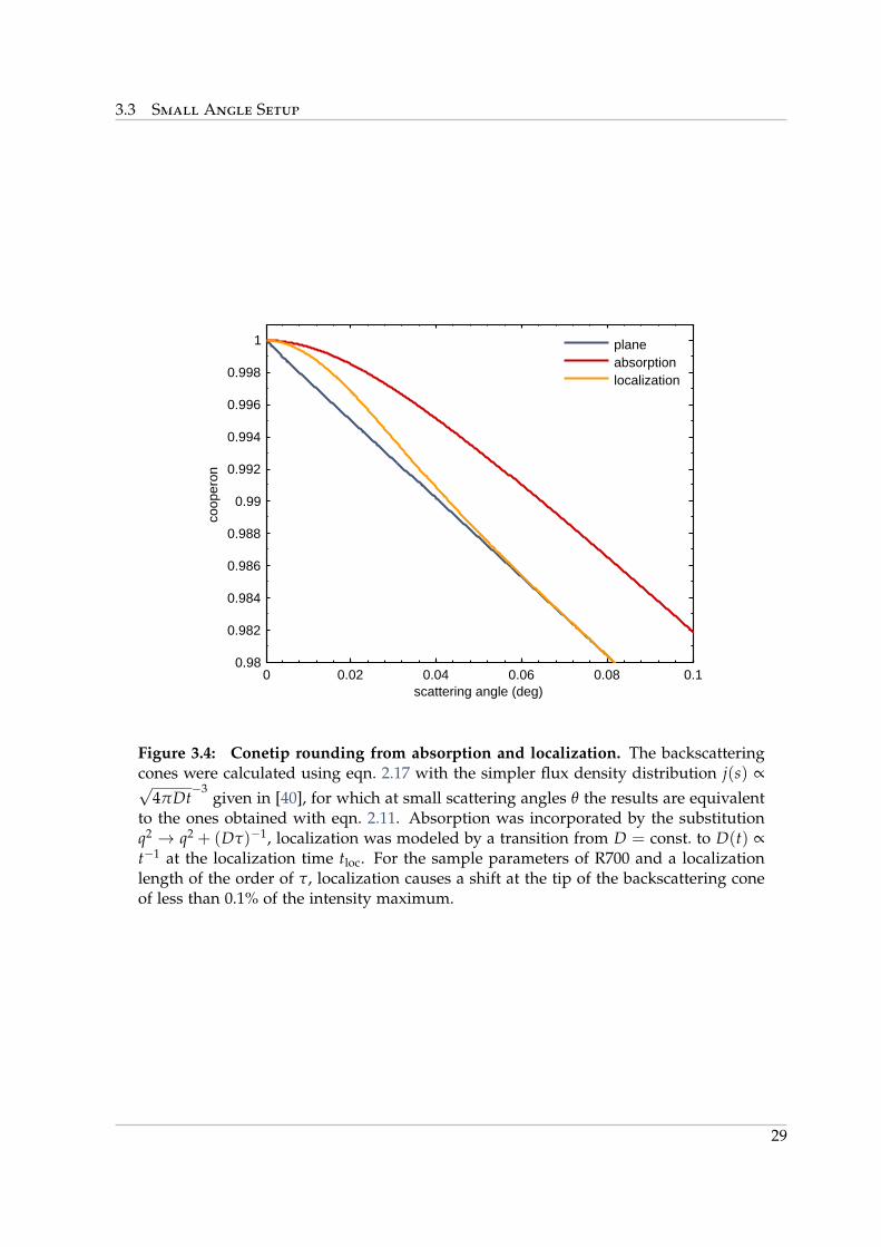
Test calculations show that the intensity difference between a localizing and a non-localizingsample is less than 0.1% of the maximum of the cooperon (fig. 3.4). As the detection mustbe able to capture the maximal backscattered intensity at θ = 0, plus some external radiationand electronic noise that can never be avoided completely, while still providing the necessaryintensity resolution, the digital range of the detection must be at least 214, better 215 − 216.
3.3.2 Optical setup
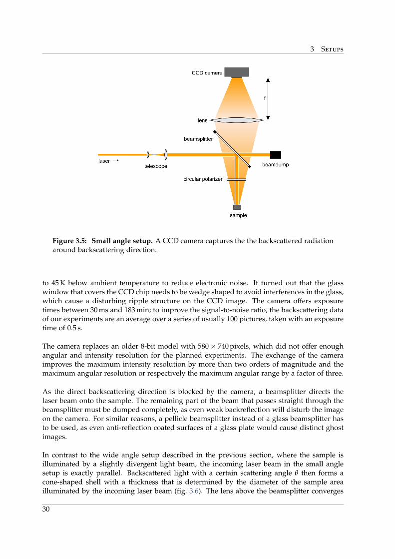
In the small angle setup a 4-megapixel 16-bit monochrome CCD camera (Alta U4000 fromApogee) is placed opposite the sample (fig. 3.5). The camera can be cooled thermoelectrically
28
3.3 Small Angle Setup
0 0.02 0.04 0.06 0.08 0.10.98
0.982
0.984
0.986
0.988
0.99
0.992
0.994
0.996
0.998
1
scattering angle (deg)
coop
eron
planeabsorptionlocalization
Figure 3.4: Conetip rounding from absorption and localization. The backscatteringcones were calculated using eqn. 2.17 with the simpler flux density distribution j(s) ∝√
4πDt−3
given in [40], for which at small scattering angles θ the results are equivalentto the ones obtained with eqn. 2.11. Absorption was incorporated by the substitutionq2 → q2 + (Dτ)−1, localization was modeled by a transition from D = const. to D(t) ∝t−1 at the localization time tloc. For the sample parameters of R700 and a localizationlength of the order of τ, localization causes a shift at the tip of the backscattering coneof less than 0.1% of the intensity maximum.
29
3 Setups
Figure 3.5: Small angle setup. A CCD camera captures the the backscattered radiationaround backscattering direction.
to 45 K below ambient temperature to reduce electronic noise. It turned out that the glasswindow that covers the CCD chip needs to be wedge shaped to avoid interferences in the glass,which cause a disturbing ripple structure on the CCD image. The camera offers exposuretimes between 30 ms and 183 min; to improve the signal-to-noise ratio, the backscattering dataof our experiments are an average over a series of usually 100 pictures, taken with an exposuretime of 0.5 s.
The camera replaces an older 8-bit model with 580× 740 pixels, which did not offer enoughangular and intensity resolution for the planned experiments. The exchange of the cameraimproves the maximum intensity resolution by more than two orders of magnitude and themaximum angular resolution or respectively the maximum angular range by a factor of three.
As the direct backscattering direction is blocked by the camera, a beamsplitter directs thelaser beam onto the sample. The remaining part of the beam that passes straight through thebeamsplitter must be dumped completely, as even weak backreflection will disturb the imageon the camera. For similar reasons, a pellicle beamsplitter instead of a glass beamsplitter hasto be used, as even anti-reflection coated surfaces of a glass plate would cause distinct ghostimages.
In contrast to the wide angle setup described in the previous section, where the sample isilluminated by a slightly divergent light beam, the incoming laser beam in the small anglesetup is exactly parallel. Backscattered light with a certain scattering angle θ then forms acone-shaped shell with a thickness that is determined by the diameter of the sample areailluminated by the incoming laser beam (fig. 3.6). The lens above the beamsplitter converges
30

3.3 Small Angle Setup
Figure 3.6: The optical setup. Backscattered light with a certain scattering angle θforms a cone-shaped shell, which is converged in the focal plane on a circle with radiusr by the lens with focal length f .
this ring of light on a circle in the focal plane, the radius of which is given by
r = f · tan θ (3.1)
where f is the focal length of the lens.
Like in the wide angle setup, single scattering is blocked by a circular polarizer. In the smallangle setup it is unnecessary to have a bendable polarizer foil, so a high-quality circularpolarizer from an industrial optics manufacturer (AUC circular polarizer from B+W) can beused. These are available with larger diameters than usual polarizers offered by laboratorysuppliers and provide extinction ratios up to 4000:1 [1].
3.3.3 Sample average
Solid samples like teflon or the titania powders have to be moved during the measurement toaverage over the speckle pattern. The method used in the wide angle setup, where the sampleis simply rotated, however turned out to be inconvenient as the high-resolving camera pickedup this rotational motion as a circular structure in the images. To have a larger ensemble toaverage over in the small angle experiments, the sample is therefore pulled on Lissajous loopsby two motors with a frequency of several Hertz on each axis (fig. 3.7).
3.3.4 Data evaluation
For the evaluation of the backscattering data the exact position of the tip of the coherentbackscattering cone at θ = 0 has to be obtained from the CCD image. We do this by converting
31
3 Setups
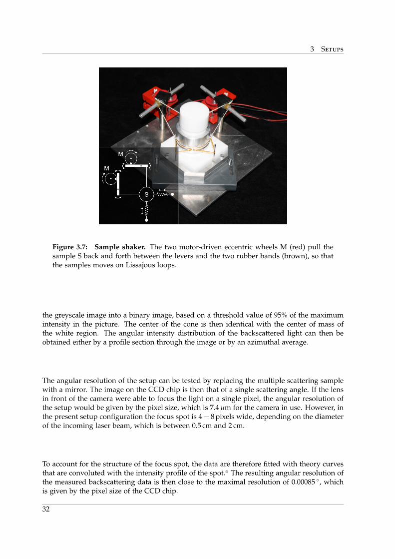
Figure 3.7: Sample shaker. The two motor-driven eccentric wheels M (red) pull thesample S back and forth between the levers and the two rubber bands (brown), so thatthe samples moves on Lissajous loops.
the greyscale image into a binary image, based on a threshold value of 95% of the maximumintensity in the picture. The center of the cone is then identical with the center of mass ofthe white region. The angular intensity distribution of the backscattered light can then beobtained either by a profile section through the image or by an azimuthal average.
The angular resolution of the setup can be tested by replacing the multiple scattering samplewith a mirror. The image on the CCD chip is then that of a single scattering angle. If the lensin front of the camera were able to focus the light on a single pixel, the angular resolution ofthe setup would be given by the pixel size, which is 7.4 µm for the camera in use. However, inthe present setup configuration the focus spot is 4− 8 pixels wide, depending on the diameterof the incoming laser beam, which is between 0.5 cm and 2 cm.
To account for the structure of the focus spot, the data are therefore fitted with theory curvesthat are convoluted with the intensity profile of the spot.a The resulting angular resolution ofthe measured backscattering data is then close to the maximal resolution of 0.00085 , whichis given by the pixel size of the CCD chip.
32
3.4 Time Of Flight Setup
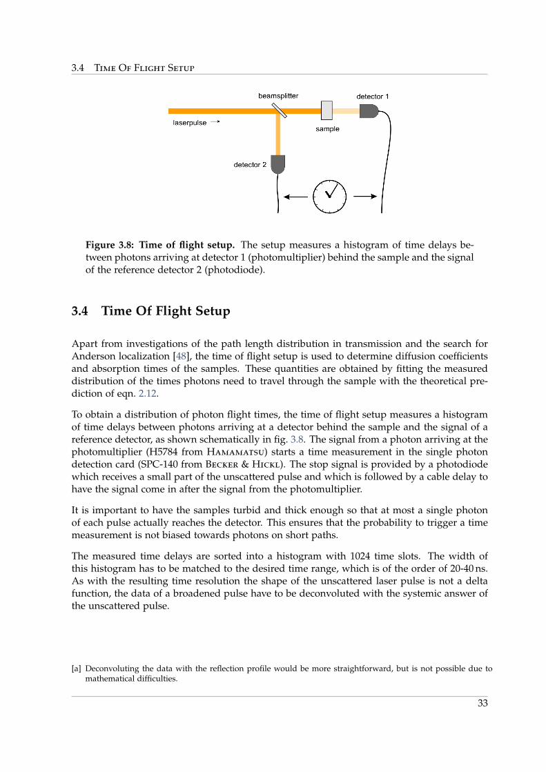
Figure 3.8: Time of flight setup. The setup measures a histogram of time delays be-tween photons arriving at detector 1 (photomultiplier) behind the sample and the signalof the reference detector 2 (photodiode).
3.4 Time Of Flight Setup
Apart from investigations of the path length distribution in transmission and the search forAnderson localization [48], the time of flight setup is used to determine diffusion coefficientsand absorption times of the samples. These quantities are obtained by fitting the measureddistribution of the times photons need to travel through the sample with the theoretical pre-diction of eqn. 2.12.
To obtain a distribution of photon flight times, the time of flight setup measures a histogramof time delays between photons arriving at a detector behind the sample and the signal of areference detector, as shown schematically in fig. 3.8. The signal from a photon arriving at thephotomultiplier (H5784 from Hamamatsu) starts a time measurement in the single photondetection card (SPC-140 from Becker & Hickl). The stop signal is provided by a photodiodewhich receives a small part of the unscattered pulse and which is followed by a cable delay tohave the signal come in after the signal from the photomultiplier.
It is important to have the samples turbid and thick enough so that at most a single photonof each pulse actually reaches the detector. This ensures that the probability to trigger a timemeasurement is not biased towards photons on short paths.
The measured time delays are sorted into a histogram with 1024 time slots. The width ofthis histogram has to be matched to the desired time range, which is of the order of 20-40 ns.As with the resulting time resolution the shape of the unscattered laser pulse is not a deltafunction, the data of a broadened pulse have to be deconvoluted with the systemic answer ofthe unscattered pulse.
[a] Deconvoluting the data with the reflection profile would be more straightforward, but is not possible due tomathematical difficulties.
33

3 Setups
34
4 Samples
4.1 Sample characterization techniques
The light scattering experiments performed with the setups introduced in sec. 3 are the mainsource of data which characterize the multiple scattering samples. However, there are a fewadditional sample properties which have to be obtained otherwise. These are mainly theeffective refractive index of the sample and the reflectivity of the sample surface, which arenecessary for example to calculate the average penetration depth z0. Also important are theparticle size and polydispersity of the samples and the filling fraction of the sample. Someof these calculations are trivial and can be found in every physics textbook, but still are to bementioned briefly.
4.1.1 Particle size and polydispersity
Particle size and polydispersity of the the colloidal particles give first indications for the scat-tering properties of the multiple scattering samples. Strongly scattering samples have particlediameters of the order of the wavelength and low polydispersity. Especially strong scatteringis obtained when the scattering in the particles becomes resonant.
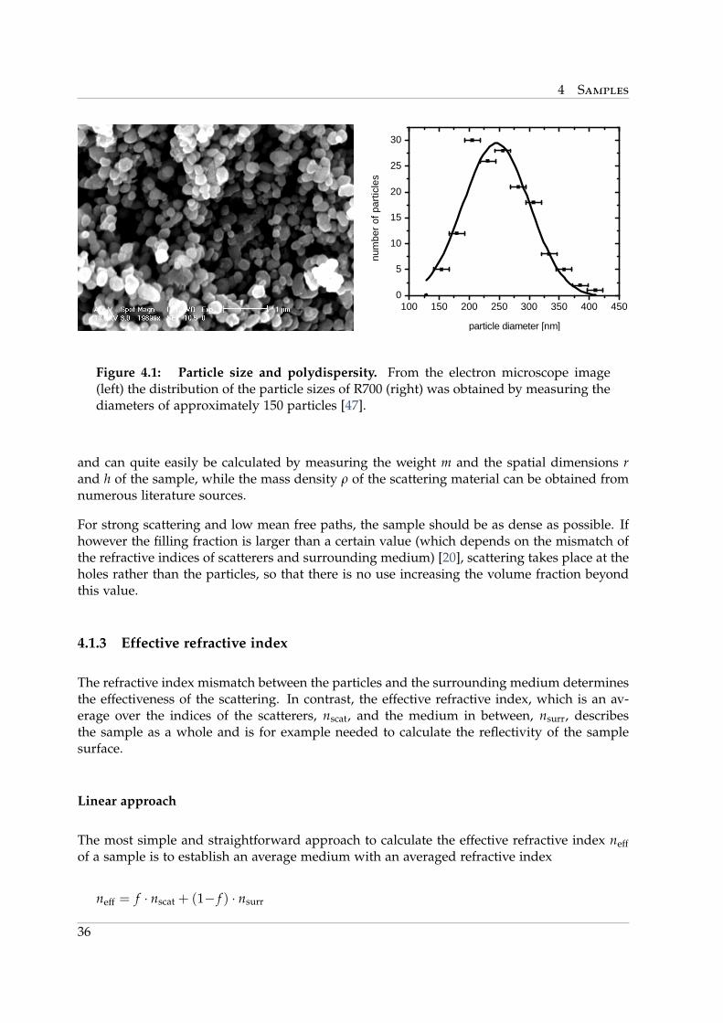
The commercial titanium dioxide samples have been characterized before by M. Storzer [47],who used electron microscopy to determine size and polydispersity of the particles. Thedevice used was an XL Scanning Electron Microscope from Phillips, which provides a spatialresolution of up to 50 nm. To avoid charge building in the sample the surface was covered witha gold layer of approximately 10 nm thickness, which was brought onto the sample using agas discharge sputter technique (Scancoat SIX, Edwards). The distribution of the particle sizeswas obtained by measuring the diameters of 150-200 particles from the pictures (fig 4.1).
4.1.2 Filling fraction
Another important feature is the filling fraction of the scatterers, which not only characterizesthe sample for itself, but is also needed for calculating the effective refractive index of thesample.
The filling fraction is defined as
f =Vscatterers
Vsample=
mρ · r2πh
4 Samples
1 0 0 1 5 0 2 0 0 2 5 0 3 0 0 3 5 0 4 0 0 4 5 00
5
1 0
1 5
2 0
2 5
3 0
numb
er of
partic
les
p a r t i c l e d i a m e t e r [ n m ]
Figure 4.1: Particle size and polydispersity. From the electron microscope image(left) the distribution of the particle sizes of R700 (right) was obtained by measuring thediameters of approximately 150 particles [47].
and can quite easily be calculated by measuring the weight m and the spatial dimensions rand h of the sample, while the mass density ρ of the scattering material can be obtained fromnumerous literature sources.
For strong scattering and low mean free paths, the sample should be as dense as possible. Ifhowever the filling fraction is larger than a certain value (which depends on the mismatch ofthe refractive indices of scatterers and surrounding medium) [20], scattering takes place at theholes rather than the particles, so that there is no use increasing the volume fraction beyondthis value.
4.1.3 Effective refractive index
The refractive index mismatch between the particles and the surrounding medium determinesthe effectiveness of the scattering. In contrast, the effective refractive index, which is an av-erage over the indices of the scatterers, nscat, and the medium in between, nsurr, describesthe sample as a whole and is for example needed to calculate the reflectivity of the samplesurface.
Linear approach
The most simple and straightforward approach to calculate the effective refractive index neffof a sample is to establish an average medium with an averaged refractive index
neff = f · nscat + (1− f ) · nsurr
36
4.1 Sample characterization techniques
0 0.2 0.4 0.6 0.8 1
1
1.5
2
2.5
3
filling fraction
refr
activ
e in
dex
linearGarnett
Figure 4.2: Refractive index. The results of the theory of J. C. M. Garnett differsfrom the linear approach especially for volume fractions around 50%. The refractiveindices in the graph were calculated for scatterers with refractive index nsc = 2.7 anda surrounding medium with nm = 1. The maximal difference is found for f = 50.4%,where the refractive index calculated with the linear approach is about 16% larger thanwith Garnett’s theory [49].
This approach works well as long as the microscopic structure of the sample is much smallerthan the wavelength. However, it must fail as soon as the complicated interactions of theinhomogenous material distribution start to matter.
Garnett effective refractive index
The theory of J. C. M. Garnett [21] calculates the average electrical field inside the mediumassuming that the fields in the scatterers and in the embedding matrix are related linearly. Ityields an effective dielectric constant
εeff = εsurr ·(
1 +3 f · εscat−εsurr
εscat+2εsurr
1− f · εscat−εsurrεscat+2εsurr
)(4.1)
for spherical scatterers. As the above assumption neglects effects like the Mie resonances, thetheory is valid only for Raleigh scatterers, or for samples with rather high polydispersity orirregularly shaped particles, where resonant effects average out. As the latter is true for thesamples used in this work, Garnett’s theory will be used to calculate the refractive index.
4.1.4 Surface reflectivity
Reflections at the sample surfaces strongly influence the distribution of the photon densityinside [58]. The angle dependent reflectivity of the boundary between the sample and the
37
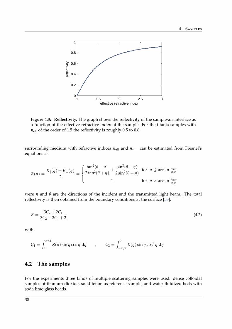
4 Samples
1 1.5 2 2.5 30
0.2
0.4
0.6
0.8
1
effective refractive index
refle
ctiv
ity
Figure 4.3: Reflectivity. The graph shows the reflectivity of the sample-air interface asa function of the effective refractive index of the sample. For the titania samples withneff of the order of 1.5 the reflectivity is roughly 0.5 to 0.6.
surrounding medium with refractive indices neff and nsurr can be estimated from Fresnel’sequations as
R(η) =R‖(η) + R⊥(η)
2=
tan2(θ − η)
2 tan2(θ + η)+
sin2(θ − η)
2 sin2(θ + η)for η ≤ arcsin nsurr
neff
1 for η > arcsin nsurrneff
were η and θ are the directions of the incident and the transmitted light beam. The totalreflectivity is then obtained from the boundary conditions at the surface [58]:
R =3C2 + 2C1
3C2 − 2C1 + 2(4.2)
with
C1 =∫ π/2
0R(η) sin η cos η dη , C2 =
∫ 0
−π/2R(η) sin η cos2 η dη
4.2 The samples
For the experiments three kinds of multiple scattering samples were used: dense colloidalsamples of titanium dioxide, solid teflon as reference sample, and water-fluidized beds withsoda lime glass beads.
38
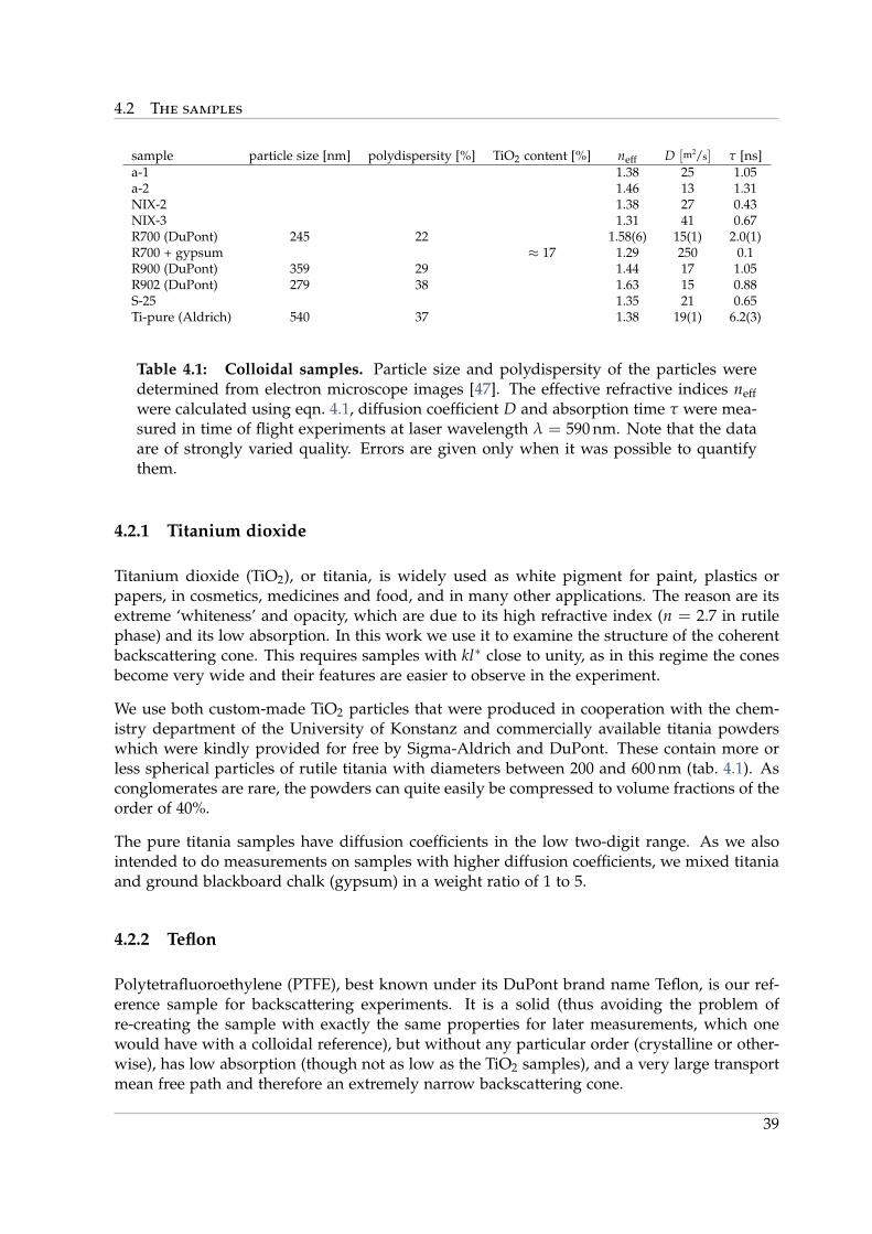
4.2 The samples
sample particle size [nm] polydispersity [%] TiO2 content [%] neff D [m2/s] τ [ns]a-1 1.38 25 1.05a-2 1.46 13 1.31NIX-2 1.38 27 0.43NIX-3 1.31 41 0.67R700 (DuPont) 245 22 1.58(6) 15(1) 2.0(1)R700 + gypsum ≈ 17 1.29 250 0.1R900 (DuPont) 359 29 1.44 17 1.05R902 (DuPont) 279 38 1.63 15 0.88S-25 1.35 21 0.65Ti-pure (Aldrich) 540 37 1.38 19(1) 6.2(3)
Table 4.1: Colloidal samples. Particle size and polydispersity of the particles weredetermined from electron microscope images [47]. The effective refractive indices neffwere calculated using eqn. 4.1, diffusion coefficient D and absorption time τ were mea-sured in time of flight experiments at laser wavelength λ = 590 nm. Note that the dataare of strongly varied quality. Errors are given only when it was possible to quantifythem.
4.2.1 Titanium dioxide
Titanium dioxide (TiO2), or titania, is widely used as white pigment for paint, plastics orpapers, in cosmetics, medicines and food, and in many other applications. The reason are itsextreme ‘whiteness’ and opacity, which are due to its high refractive index (n = 2.7 in rutilephase) and its low absorption. In this work we use it to examine the structure of the coherentbackscattering cone. This requires samples with kl∗ close to unity, as in this regime the conesbecome very wide and their features are easier to observe in the experiment.
We use both custom-made TiO2 particles that were produced in cooperation with the chem-istry department of the University of Konstanz and commercially available titania powderswhich were kindly provided for free by Sigma-Aldrich and DuPont. These contain more orless spherical particles of rutile titania with diameters between 200 and 600 nm (tab. 4.1). Asconglomerates are rare, the powders can quite easily be compressed to volume fractions of theorder of 40%.
The pure titania samples have diffusion coefficients in the low two-digit range. As we alsointended to do measurements on samples with higher diffusion coefficients, we mixed titaniaand ground blackboard chalk (gypsum) in a weight ratio of 1 to 5.
4.2.2 Teflon
Polytetrafluoroethylene (PTFE), best known under its DuPont brand name Teflon, is our ref-erence sample for backscattering experiments. It is a solid (thus avoiding the problem ofre-creating the sample with exactly the same properties for later measurements, which onewould have with a colloidal reference), but without any particular order (crystalline or other-wise), has low absorption (though not as low as the TiO2 samples), and a very large transportmean free path and therefore an extremely narrow backscattering cone.
39
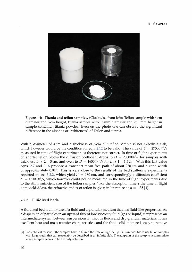
4 Samples
Figure 4.4: Titania and teflon samples. (Clockwise from left:) Teflon sample with 4 cmdiameter and 5 cm height, titania sample with 15 mm diameter and < 1 mm height insample container, titania powder. Even on the photo one can observe the significantdifference in the albedos or ”whiteness” of Teflon and titania.
With a diameter of 4 cm and a thickness of 5 cm our teflon sample is not exactly a slab,which however would be the condition for eqn. 2.12 to be valid. The value of D = 27500 m2/s
measured in time of flight experiments is therefore not correct. In time of flight experimentson shorter teflon blocks the diffusion coefficient drops to D = 20000 m2/s for samples withthickness L ≈ 2− 3 cm, and even to D = 16500 m2/s for L ≈ 1− 1.5 cm. With this last valueeqns. 2.7 and 2.16 propose a transport mean free path of about 220 µm and a cone widthof approximately 0.01. This is very close to the results of the backscattering experimentsreported in sec. 5.2.2, which yield l∗ = 180 µm, and correspondingly a diffusion coefficientD = 13300 m2/s, which however could not be measured in the time of flight experiments dueto the still insufficient size of the teflon samples.a For the absorption time τ the time of flightdata yield 3.3 ns, the refractive index of teflon is given in literature as n = 1.35 [4].
4.2.3 Fluidized beds
A fluidized bed is a mixture of a fluid and a granular medium that has fluid-like properties. Asa dispersion of particles in an upward flux of low-viscosity fluid (gas or liquid) it represents anintermediate system between suspensions in viscous fluids and dry granular materials. It hasexcellent heat and mass transfer characteristics, and the fluid-solid mixture is easy to remove
[a] For technical reasons – the samples have to fit into the time of flight setup – it is impossible to use teflon sampleswith larger radii that can reasonably be described as an infinite slab. The adaption of the setup to accommodatelarger samples seems to be the only solution.
40
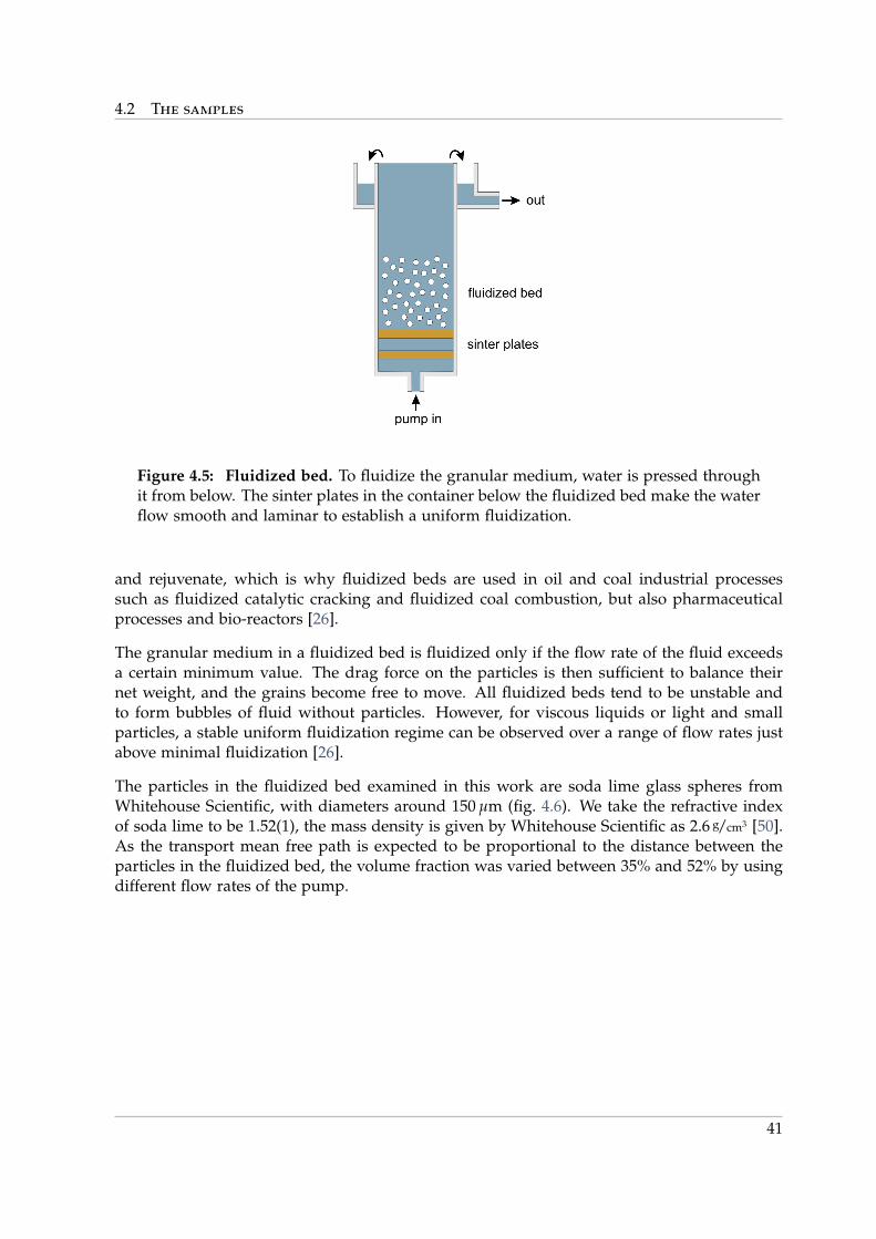
4.2 The samples
Figure 4.5: Fluidized bed. To fluidize the granular medium, water is pressed throughit from below. The sinter plates in the container below the fluidized bed make the waterflow smooth and laminar to establish a uniform fluidization.
and rejuvenate, which is why fluidized beds are used in oil and coal industrial processessuch as fluidized catalytic cracking and fluidized coal combustion, but also pharmaceuticalprocesses and bio-reactors [26].
The granular medium in a fluidized bed is fluidized only if the flow rate of the fluid exceedsa certain minimum value. The drag force on the particles is then sufficient to balance theirnet weight, and the grains become free to move. All fluidized beds tend to be unstable andto form bubbles of fluid without particles. However, for viscous liquids or light and smallparticles, a stable uniform fluidization regime can be observed over a range of flow rates justabove minimal fluidization [26].
The particles in the fluidized bed examined in this work are soda lime glass spheres fromWhitehouse Scientific, with diameters around 150 µm (fig. 4.6). We take the refractive indexof soda lime to be 1.52(1), the mass density is given by Whitehouse Scientific as 2.6 g/cm3 [50].As the transport mean free path is expected to be proportional to the distance between theparticles in the fluidized bed, the volume fraction was varied between 35% and 52% by usingdifferent flow rates of the pump.
41
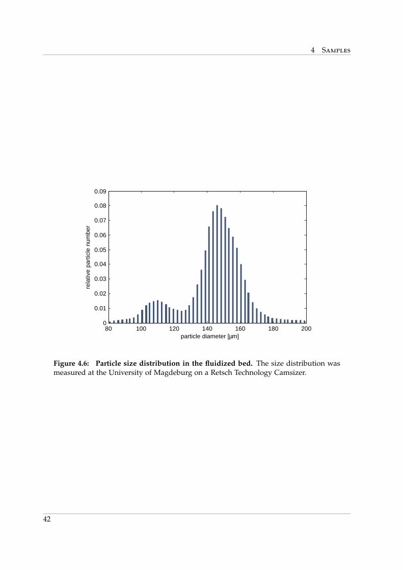
4 Samples
80 100 120 140 160 180 2000
0.01
0.02
0.03
0.04
0.05
0.06
0.07
0.08
0.09
particle diameter [µm]
rela
tive
part
icle
num
ber
Figure 4.6: Particle size distribution in the fluidized bed. The size distribution wasmeasured at the University of Magdeburg on a Retsch Technology Camsizer.
42
5 Experiments
5.1 Conservation of energy in coherent backscattering
Conservation of energy is one of the most fundamental principles in physics. However, theintensity enhancement of the coherent backscattering cone is one instance where it seems tobe violated at first glance:
The origin of the backscattering enhancement lies in the interference of waves propagatingalong reciprocal paths.a This interference can only spatially re-distribute the light energy thatemerges from the sample surface; it can not destroy photons or create new ones. The totalamount of energy per unit time emerging from the sample must therefore be the same withand without interference:
∫half-space
αd(θ) dΩ =∫
half-spaceαd(θ) + αc(θ) dΩ
where diffuson αd(θ) and cooperon αc(θ) are the coherent and the incoherent addition of thephoton flux as defined in sec. 2.7. It follows for the coherent backscattering enhancement that
∫half-space
αc(θ) dΩ = 0 (5.1)
Thus the intensity enhancement of the coherent backscattering cone at small angles should bebalanced by a corresponding intensity cutback to ensure conservation of energy.
Unfortunately, such an intensity cutback had never been observed experimentally, and thetheory of coherent backscattering as developed in sec. 2.7 does not predict an intensity cut-back either. As the principle of conservation of energy holds in any case, the only possi-ble conclusion is that both the experimental procedure and the theoretical description of thebackscattering cone are too inaccurate to render the cone correctly.
The question if the backscattering cone is depicted correctly by experiment and theory is notjust of purely academic interest. The accurate measurement and description of the cone isimportant as the scaling of its width with the inverse product of the wave vector k of thescattered light and the transport mean free path l∗ is commonly used to characterize multiplescattering materials. In particular in the study of Anderson localization of light [13] a reliable
[a] The interference nature of coherent backscattering can be proved for example by the influence of Faradayrotation on the backscattering cone [35, 36, 37].
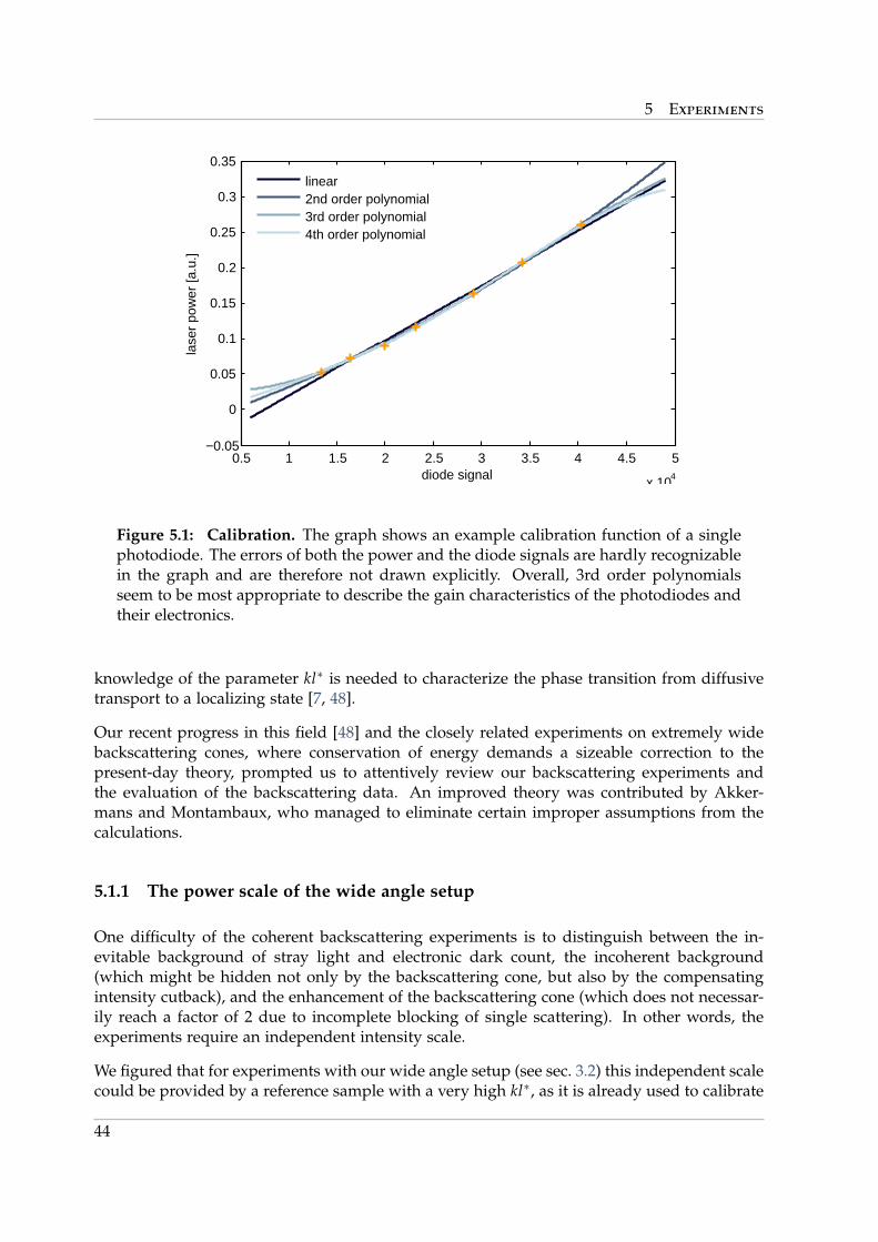
5 Experiments
0.5 1 1.5 2 2.5 3 3.5 4 4.5 5
x 104
−0.05
0
0.05
0.1
0.15
0.2
0.25
0.3
0.35
diode signal
lase
r po
wer
[a.u
.]
linear2nd order polynomial3rd order polynomial4th order polynomial
Figure 5.1: Calibration. The graph shows an example calibration function of a singlephotodiode. The errors of both the power and the diode signals are hardly recognizablein the graph and are therefore not drawn explicitly. Overall, 3rd order polynomialsseem to be most appropriate to describe the gain characteristics of the photodiodes andtheir electronics.
knowledge of the parameter kl∗ is needed to characterize the phase transition from diffusivetransport to a localizing state [7, 48].
Our recent progress in this field [48] and the closely related experiments on extremely widebackscattering cones, where conservation of energy demands a sizeable correction to thepresent-day theory, prompted us to attentively review our backscattering experiments andthe evaluation of the backscattering data. An improved theory was contributed by Akker-mans and Montambaux, who managed to eliminate certain improper assumptions from thecalculations.
5.1.1 The power scale of the wide angle setup
One difficulty of the coherent backscattering experiments is to distinguish between the in-evitable background of stray light and electronic dark count, the incoherent background(which might be hidden not only by the backscattering cone, but also by the compensatingintensity cutback), and the enhancement of the backscattering cone (which does not necessar-ily reach a factor of 2 due to incomplete blocking of single scattering). In other words, theexperiments require an independent intensity scale.
We figured that for experiments with our wide angle setup (see sec. 3.2) this independent scalecould be provided by a reference sample with a very high kl∗, as it is already used to calibrate
44
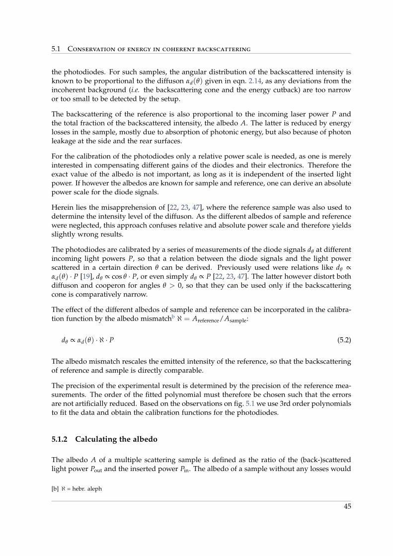
5.1 Conservation of energy in coherent backscattering
the photodiodes. For such samples, the angular distribution of the backscattered intensity isknown to be proportional to the diffuson αd(θ) given in eqn. 2.14, as any deviations from theincoherent background (i.e. the backscattering cone and the energy cutback) are too narrowor too small to be detected by the setup.
The backscattering of the reference is also proportional to the incoming laser power P andthe total fraction of the backscattered intensity, the albedo A. The latter is reduced by energylosses in the sample, mostly due to absorption of photonic energy, but also because of photonleakage at the side and the rear surfaces.
For the calibration of the photodiodes only a relative power scale is needed, as one is merelyinterested in compensating different gains of the diodes and their electronics. Therefore theexact value of the albedo is not important, as long as it is independent of the inserted lightpower. If however the albedos are known for sample and reference, one can derive an absolutepower scale for the diode signals.
Herein lies the misapprehension of [22, 23, 47], where the reference sample was also used todetermine the intensity level of the diffuson. As the different albedos of sample and referencewere neglected, this approach confuses relative and absolute power scale and therefore yieldsslightly wrong results.
The photodiodes are calibrated by a series of measurements of the diode signals dθ at differentincoming light powers P, so that a relation between the diode signals and the light powerscattered in a certain direction θ can be derived. Previously used were relations like dθ ∝αd(θ) · P [19], dθ ∝ cos θ · P, or even simply dθ ∝ P [22, 23, 47]. The latter however distort bothdiffuson and cooperon for angles θ > 0, so that they can be used only if the backscatteringcone is comparatively narrow.
The effect of the different albedos of sample and reference can be incorporated in the calibra-tion function by the albedo mismatchb ℵ = Areference/Asample:
dθ ∝ αd(θ) · ℵ · P (5.2)
The albedo mismatch rescales the emitted intensity of the reference, so that the backscatteringof reference and sample is directly comparable.
The precision of the experimental result is determined by the precision of the reference mea-surements. The order of the fitted polynomial must therefore be chosen such that the errorsare not artificially reduced. Based on the observations on fig. 5.1 we use 3rd order polynomialsto fit the data and obtain the calibration functions for the photodiodes.
5.1.2 Calculating the albedo
The albedo A of a multiple scattering sample is defined as the ratio of the (back-)scatteredlight power Pout and the inserted power Pin. The albedo of a sample without any losses would
[b] ℵ = hebr. aleph
45
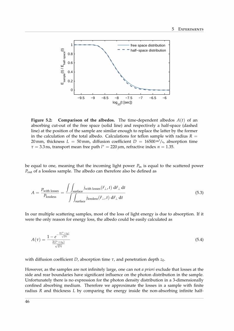
5 Experiments
−9.5 −9 −8.5 −8 −7.5 −7 −6.5 −6
0
0.2
0.4
0.6
0.8
1
log10
(t [sec])
Esa
mpl
e(t)
/ Eha
lf−sp
ace(t
)
free space distributionhalf−space distribution
Figure 5.2: Comparison of the albedos. The time-dependent albedos A(t) of anabsorbing cut-out of the free space (solid line) and respectively a half-space (dashedline) at the position of the sample are similar enough to replace the latter by the formerin the calculation of the total albedo. Calculations for teflon sample with radius R =20 mm, thickness L = 50 mm, diffusion coefficient D = 16500 m2/s, absorption timeτ = 3.3 ns, transport mean free path l∗ = 220 µm, refractive index n = 1.35.
be equal to one, meaning that the incoming light power Pin is equal to the scattered powerPout of a lossless sample. The albedo can therefore also be defined as
A =Pwith losses
Plossless=
∫ ∫surface
jwith losses(~r⊥, t) d~r⊥ dt∫ ∫surface
jlossless(~r⊥, t) d~r⊥ dt(5.3)
In our multiple scattering samples, most of the loss of light energy is due to absorption. If itwere the only reason for energy loss, the albedo could be easily calculated as
A(τ) =1− e−
2(l∗+z0)√Dτ
2(l∗+z0)√Dτ
(5.4)
with diffusion coefficient D, absorption time τ, and penetration depth z0.
However, as the samples are not infinitely large, one can not a priori exclude that losses at theside and rear boundaries have significant influence on the photon distribution in the sample.Unfortunately there is no expression for the photon density distribution in a 3-dimensionallyconfined absorbing medium. Therefore we approximate the losses in a sample with finiteradius R and thickness L by comparing the energy inside the non-absorbing infinite half-
46
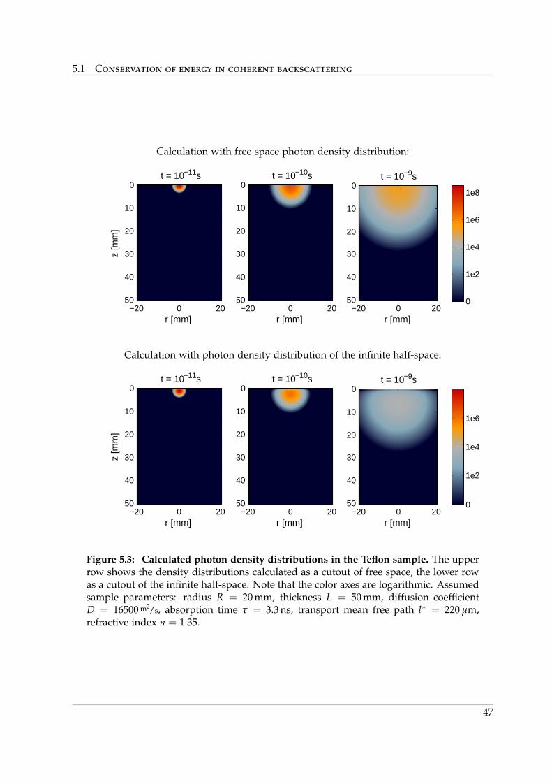
5.1 Conservation of energy in coherent backscattering
Calculation with free space photon density distribution:
t = 10−11s
r [mm]
z [m
m]
−20 0 20
0
10
20
30
40
50
t = 10−10s
r [mm]−20 0 20
0
10
20
30
40
50
t = 10−9s
r [mm]
−20 0 20
0
10
20
30
40
50 0
1e2
1e4
1e6
1e8
Calculation with photon density distribution of the infinite half-space:
t = 10−11s
r [mm]
z [m
m]
−20 0 20
0
10
20
30
40
50
t = 10−10s
r [mm]−20 0 20
0
10
20
30
40
50
t = 10−9s
r [mm]
−20 0 20
0
10
20
30
40
50 0
1e2
1e4
1e6
Figure 5.3: Calculated photon density distributions in the Teflon sample. The upperrow shows the density distributions calculated as a cutout of free space, the lower rowas a cutout of the infinite half-space. Note that the color axes are logarithmic. Assumedsample parameters: radius R = 20 mm, thickness L = 50 mm, diffusion coefficientD = 16500 m2/s, absorption time τ = 3.3 ns, transport mean free path l∗ = 220 µm,refractive index n = 1.35.
47
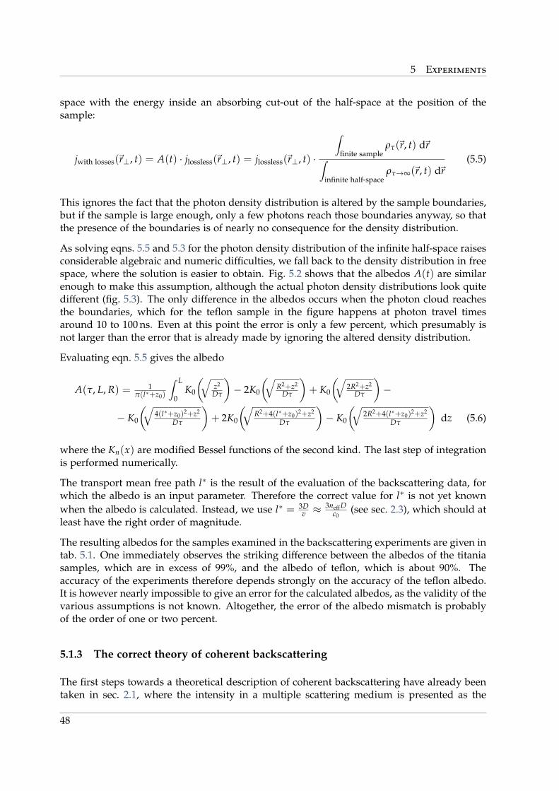
5 Experiments
space with the energy inside an absorbing cut-out of the half-space at the position of thesample:
jwith losses(~r⊥, t) = A(t) · jlossless(~r⊥, t) = jlossless(~r⊥, t) ·
∫finite sample
ρτ(~r, t) d~r∫infinite half-space
ρτ→∞(~r, t) d~r(5.5)
This ignores the fact that the photon density distribution is altered by the sample boundaries,but if the sample is large enough, only a few photons reach those boundaries anyway, so thatthe presence of the boundaries is of nearly no consequence for the density distribution.
As solving eqns. 5.5 and 5.3 for the photon density distribution of the infinite half-space raisesconsiderable algebraic and numeric difficulties, we fall back to the density distribution in freespace, where the solution is easier to obtain. Fig. 5.2 shows that the albedos A(t) are similarenough to make this assumption, although the actual photon density distributions look quitedifferent (fig. 5.3). The only difference in the albedos occurs when the photon cloud reachesthe boundaries, which for the teflon sample in the figure happens at photon travel timesaround 10 to 100 ns. Even at this point the error is only a few percent, which presumably isnot larger than the error that is already made by ignoring the altered density distribution.
Evaluating eqn. 5.5 gives the albedo
A(τ, L, R) = 1π(l∗+z0)
∫ L
0K0
(√z2
Dτ
)− 2K0
(√R2+z2
Dτ
)+ K0
(√2R2+z2
Dτ
)−
− K0
(√4(l∗+z0)
2+z2
Dτ
)+ 2K0
(√R2+4(l∗+z0)
2+z2
Dτ
)− K0
(√2R2+4(l∗+z0)
2+z2
Dτ
)dz (5.6)
where the Kn(x) are modified Bessel functions of the second kind. The last step of integrationis performed numerically.
The transport mean free path l∗ is the result of the evaluation of the backscattering data, forwhich the albedo is an input parameter. Therefore the correct value for l∗ is not yet knownwhen the albedo is calculated. Instead, we use l∗ = 3D
v ≈3neffD
c0(see sec. 2.3), which should at
least have the right order of magnitude.
The resulting albedos for the samples examined in the backscattering experiments are given intab. 5.1. One immediately observes the striking difference between the albedos of the titaniasamples, which are in excess of 99%, and the albedo of teflon, which is about 90%. Theaccuracy of the experiments therefore depends strongly on the accuracy of the teflon albedo.It is however nearly impossible to give an error for the calculated albedos, as the validity of thevarious assumptions is not known. Altogether, the error of the albedo mismatch is probablyof the order of one or two percent.
5.1.3 The correct theory of coherent backscattering
The first steps towards a theoretical description of coherent backscattering have already beentaken in sec. 2.1, where the intensity in a multiple scattering medium is presented as the
48
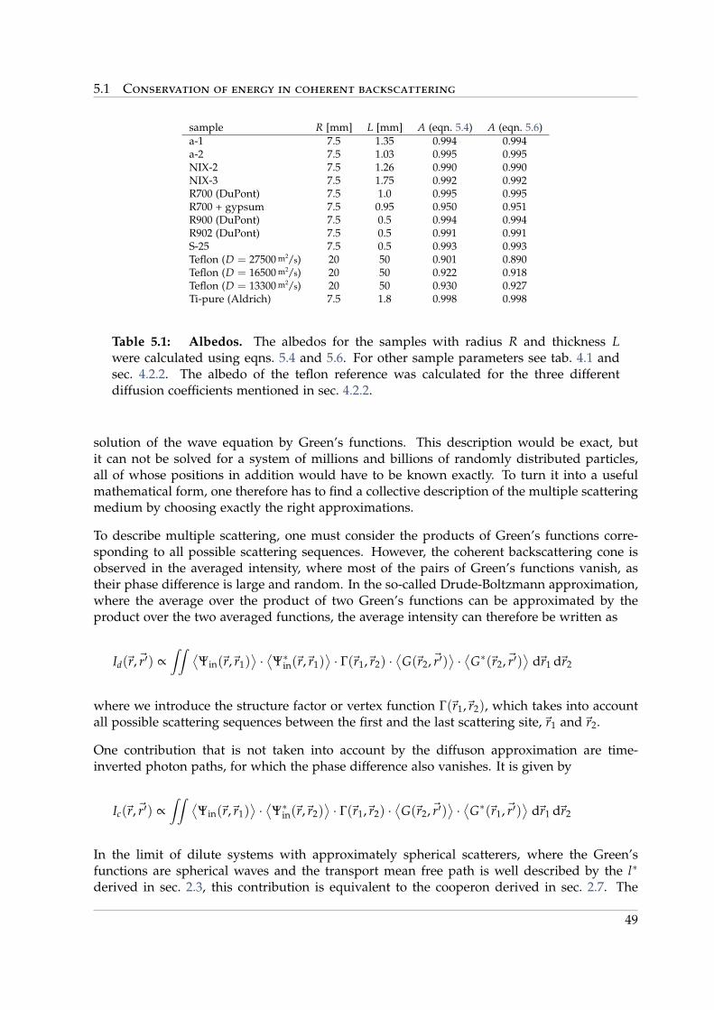
5.1 Conservation of energy in coherent backscattering
sample R [mm] L [mm] A (eqn. 5.4) A (eqn. 5.6)a-1 7.5 1.35 0.994 0.994a-2 7.5 1.03 0.995 0.995NIX-2 7.5 1.26 0.990 0.990NIX-3 7.5 1.75 0.992 0.992R700 (DuPont) 7.5 1.0 0.995 0.995R700 + gypsum 7.5 0.95 0.950 0.951R900 (DuPont) 7.5 0.5 0.994 0.994R902 (DuPont) 7.5 0.5 0.991 0.991S-25 7.5 0.5 0.993 0.993Teflon (D = 27500 m2/s) 20 50 0.901 0.890Teflon (D = 16500 m2/s) 20 50 0.922 0.918Teflon (D = 13300 m2/s) 20 50 0.930 0.927Ti-pure (Aldrich) 7.5 1.8 0.998 0.998
Table 5.1: Albedos. The albedos for the samples with radius R and thickness Lwere calculated using eqns. 5.4 and 5.6. For other sample parameters see tab. 4.1 andsec. 4.2.2. The albedo of the teflon reference was calculated for the three differentdiffusion coefficients mentioned in sec. 4.2.2.
solution of the wave equation by Green’s functions. This description would be exact, butit can not be solved for a system of millions and billions of randomly distributed particles,all of whose positions in addition would have to be known exactly. To turn it into a usefulmathematical form, one therefore has to find a collective description of the multiple scatteringmedium by choosing exactly the right approximations.
To describe multiple scattering, one must consider the products of Green’s functions corre-sponding to all possible scattering sequences. However, the coherent backscattering cone isobserved in the averaged intensity, where most of the pairs of Green’s functions vanish, astheir phase difference is large and random. In the so-called Drude-Boltzmann approximation,where the average over the product of two Green’s functions can be approximated by theproduct over the two averaged functions, the average intensity can therefore be written as
Id(~r,~r′) ∝∫∫ ⟨
Ψin(~r,~r1)⟩·⟨Ψ∗in(~r,~r1)
⟩· Γ(~r1,~r2) ·
⟨G(~r2,~r′)
⟩·⟨
G∗(~r2,~r′)⟩
d~r1 d~r2
where we introduce the structure factor or vertex function Γ(~r1,~r2), which takes into accountall possible scattering sequences between the first and the last scattering site,~r1 and~r2.
One contribution that is not taken into account by the diffuson approximation are time-inverted photon paths, for which the phase difference also vanishes. It is given by
Ic(~r,~r′) ∝∫∫ ⟨
Ψin(~r,~r1)⟩·⟨Ψ∗in(~r,~r2)
⟩· Γ(~r1,~r2) ·
⟨G(~r2,~r′)
⟩·⟨
G∗(~r1,~r′)⟩
d~r1 d~r2
In the limit of dilute systems with approximately spherical scatterers, where the Green’sfunctions are spherical waves and the transport mean free path is well described by the l∗
derived in sec. 2.3, this contribution is equivalent to the cooperon derived in sec. 2.7. The
49
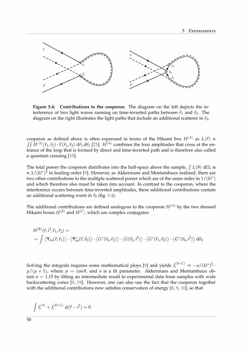
5 Experiments
Figure 5.4: Contributions to the cooperon. The diagram on the left depicts the in-terference of two light waves running on time-inverted paths between ~r1 and ~r2. Thediagram on the right illustrates the light paths that include an additional scatterer in~r0.
cooperon as defined above is often expressed in terms of the Hikami box H(A) as Ic(~r) ∝∫∫H(A)(~r1,~r2) · Γ(~r1,~r2) d~r1 d~r2 [25]. H(A) combines the four amplitudes that cross at the en-
trance of the loop that is formed by direct and time-inverted path and is therefore also calleda quantum crossing [10].
The total power the cooperon distributes into the half-space above the sample,∫
Ic(θ) dΩ, is∝ 1/(kl∗)2 in leading order [9]. However, as Akkermans and Montambaux realized, there aretwo other contributions to the multiple scattered power which are of the same order in 1/(kl∗)and which therefore also must be taken into account. In contrast to the cooperon, where theinterference occurs between time-inverted amplitudes, these additional contributions containan additional scattering event in~r0 (fig. 5.4).
The additional contributions are defined analogous to the cooperon H(A) by the two dressedHikami boxes H(B) and H(C), which are complex conjugates:
H(B)(~r,~r′,~r1,~r2) =
=∫ ⟨
Ψin(~r,~r1)⟩·⟨Ψ∗in(~r,~r0)
⟩·⟨
G∗(~r0,~r2)⟩·⟨
G(~r2,~r′)⟩·⟨
G∗(~r1,~r0)⟩·⟨
G∗(~r0,~r′)⟩
d~r0
Solving the integrals requires some mathematical ploys [9] and yields I(B+C)c ≈ −a/(kl∗)2 ·
µ/(µ + 1), where µ = cos θ, and a is a fit parameter. Akkermans and Montambaux ob-tain a = 1.15 by fitting an intermediate result to experimental data from samples with widebackscattering cones [9, 19]. However, one can also use the fact that the cooperon togetherwith the additional contributions now satisfies conservation of energy [8, 9, 10], so that
∫I(A)c + I(B+C)
c d(~r−~r′) = 0
50
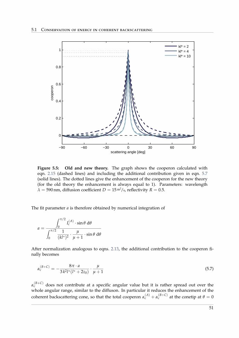
5.1 Conservation of energy in coherent backscattering
−90 −60 −30 0 30 60 90
0
0.2
0.4
0.6
0.8
1
scattering angle [deg]
coop
eron
kl* = 2kl* = 4kl* = 10
Figure 5.5: Old and new theory. The graph shows the cooperon calculated witheqn. 2.15 (dashed lines) and including the additional contribution given in eqn. 5.7(solid lines). The dotted lines give the enhancement of the cooperon for the new theory(for the old theory the enhancement is always equal to 1). Parameters: wavelengthλ = 590 nm, diffusion coefficient D = 15 m2/s, reflectivity R = 0.5.
The fit parameter a is therefore obtained by numerical integration of
a =
∫ π/2
0I(A)c · sin θ dθ∫ π/2
0
1(kl∗)2 ·
µ
µ + 1· sin θ dθ
After normalization analogous to eqns. 2.13, the additional contribution to the cooperon fi-nally becomes
α(B+C)c = − 8π · a
3 k2l∗(l∗ + 2z0)· µ
µ + 1(5.7)
α(B+C)c does not contribute at a specific angular value but it is rather spread out over the
whole angular range, similar to the diffuson. In particular it reduces the enhancement of thecoherent backscattering cone, so that the total cooperon α
(A)c + α
(B+C)c at the conetip at θ = 0
51
5 Experiments
is lower than 1 (fig. 5.5). At the wings of the backscattering cone an intensity cutback appearsthat balances the intensity enhancement of the cone.
However, the effect of α(B+C)c is significant only for small kl∗. For kl∗ ' 10 its influence is neg-
ligible, and the backscattering cone is well described by the cooperon α(A)c given in eqn. 2.15.
In this regime the diffuson can be found from the large angle wings of the backscattering data[55]. For small kl∗ the diffuson is hidden by the intensity cutback, and the proceeding devisedabove has to be used to extract the cooperon from the data.
Small kl∗ however means strongly scattering dense samples, where the scattering particles arein touching distance. In such systems, near-field effects become important for the scatteringprocess. Strictly speaking, the random walk model developed for dilute systems and thededuction of the transport mean free path from the intensity distribution of Mie scatteringand the anisotropy parameter 〈cos θ〉 are no longer valid. The kl∗ obtained by fitting with thetheory from Akkermans and Montambaux will therefore certainly have the correct order ofmagnitude, but might deviate slightly from the real value.
5.1.4 The results of the test experiments
To test the theoretical prediction made above, the coherent backscattering cones of varioussamples were measured with the wide angle setup. The diffusion coefficients lay in the rangebetween 13 m2/s and 250 m2/s (see tab. 4.1), so that we expected to observe extremely widebackscattering cones with kl∗ close to unity and a distinct intensity cutback as well as narrowcones with high kl∗ where no cutback is visible.
As the albedos of the titania samples are basically 1, the albedo mismatch of sample andreference is mainly given by the albedo of the teflon block. The latter was calculated withall three diffusion coefficients D = 27500 m2/s, D = 16500 m2/s, and D = 13300 m2/s that canbe derived from time of flight and small angle backscattering experiments, as discussed insec. 4.2.2.
The data quality of the wide angle backscattering experiments varies strongly, as the wideangle setup is extremely sensitive to parasitically scattered light. However, as stated above,the backscattering cone is evidentially caused by interference, so that the total amount ofbackscattered power must be the same both for the coherent and the incoherent addition ofthe backscattered intensity, and the integral E =
∫ 2π0
∫ π/20 ac(θ) sin θ dθ dφ of the cooperon is
necessarily zero. E can therefore be used as a criterion to judge the quality of the experimentaldata.
Furthermore, it is also possible to substantiate the method to calculate the albedo that wasdeveloped earlier. In fig. 5.6 one observes that the data are approximately centered at E = 0if the albedo is calculated with D = 16500 m2/s and D = 13300 m2/s, but are shifted to E ≈−0.1 sterad for an albedo calculated with D = 27500 m2/s. Therefore the data on averagesuggest conservation of energy for precisely those values of the diffusion coefficient whichare obtained from the small angle measurements (see sec. 5.2.2). This strongly indicates thatthe values for the albedos are correct, although as proof further experiments on samples withother albedos than teflon or titania are necessary.
52
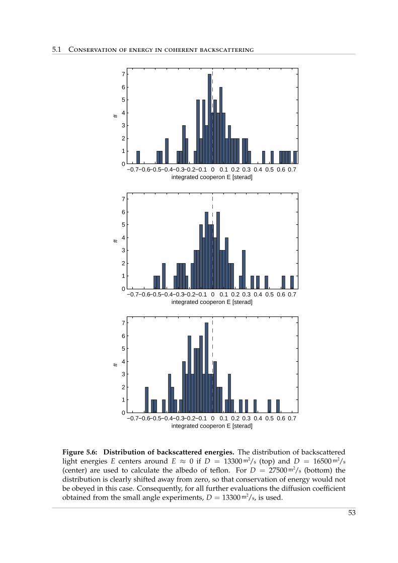
5.1 Conservation of energy in coherent backscattering
integrated cooperon E [sterad]
#
−0.7−0.6−0.5−0.4−0.3−0.2−0.1 0 0.1 0.2 0.3 0.4 0.5 0.6 0.70
1
2
3
4
5
6
7
integrated cooperon E [sterad]
#
−0.7−0.6−0.5−0.4−0.3−0.2−0.1 0 0.1 0.2 0.3 0.4 0.5 0.6 0.70
1
2
3
4
5
6
7
integrated cooperon E [sterad]
#
−0.7−0.6−0.5−0.4−0.3−0.2−0.1 0 0.1 0.2 0.3 0.4 0.5 0.6 0.70
1
2
3
4
5
6
7
Figure 5.6: Distribution of backscattered energies. The distribution of backscatteredlight energies E centers around E ≈ 0 if D = 13300 m2/s (top) and D = 16500 m2/s
(center) are used to calculate the albedo of teflon. For D = 27500 m2/s (bottom) thedistribution is clearly shifted away from zero, so that conservation of energy would notbe obeyed in this case. Consequently, for all further evaluations the diffusion coefficientobtained from the small angle experiments, D = 13300 m2/s, is used.
53
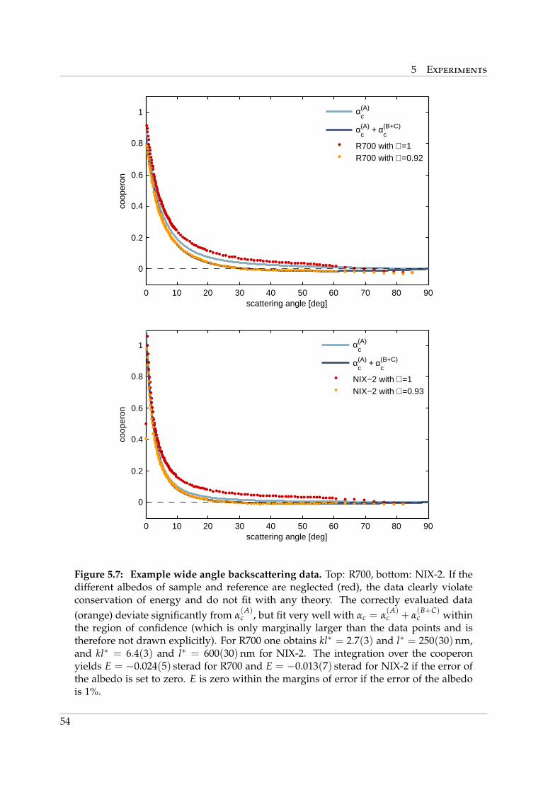
5 Experiments
0 10 20 30 40 50 60 70 80 90
0
0.2
0.4
0.6
0.8
1
scattering angle [deg]
coop
eron
αc(A)
αc(A) + α
c(B+C)
R700 with ℵ =1R700 with ℵ =0.92
0 10 20 30 40 50 60 70 80 90
0
0.2
0.4
0.6
0.8
1
scattering angle [deg]
coop
eron
αc(A)
αc(A) + α
c(B+C)
NIX−2 with ℵ =1NIX−2 with ℵ =0.93
Figure 5.7: Example wide angle backscattering data. Top: R700, bottom: NIX-2. If thedifferent albedos of sample and reference are neglected (red), the data clearly violateconservation of energy and do not fit with any theory. The correctly evaluated data(orange) deviate significantly from α
(A)c , but fit very well with αc = α
(A)c + α
(B+C)c within
the region of confidence (which is only marginally larger than the data points and istherefore not drawn explicitly). For R700 one obtains kl∗ = 2.7(3) and l∗ = 250(30) nm,and kl∗ = 6.4(3) and l∗ = 600(30) nm for NIX-2. The integration over the cooperonyields E = −0.024(5) sterad for R700 and E = −0.013(7) sterad for NIX-2 if the error ofthe albedo is set to zero. E is zero within the margins of error if the error of the albedois 1%.
54
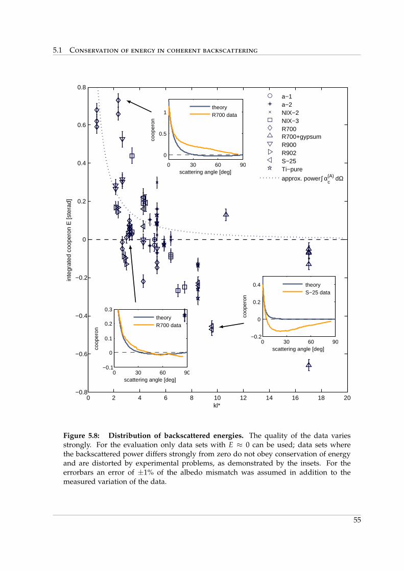
5.1 Conservation of energy in coherent backscattering
0 30 60 90−0.1
0
0.1
0.2
0.3
scattering angle [deg]
coop
eron
theoryR700 data
0 30 60 90
0
0.5
1
scattering angle [deg]
coop
eron
theoryR700 data
0 30 60 90−0.2
0
0.2
0.4
scattering angle [deg]
coop
eron
theoryS−25 data
0 2 4 6 8 10 12 14 16 18 20−0.8
−0.6
−0.4
−0.2
0
0.2
0.4
0.6
0.8
kl*
inte
grat
ed c
oope
ron
E [s
tera
d]
a−1a−2NIX−2NIX−3R700R700+gypsumR900R902S−25Ti−pure
approx. power ∫ α(A)c
dΩ
Figure 5.8: Distribution of backscattered energies. The quality of the data variesstrongly. For the evaluation only data sets with E ≈ 0 can be used; data sets wherethe backscattered power differs strongly from zero do not obey conservation of energyand are distorted by experimental problems, as demonstrated by the insets. For theerrorbars an error of ±1% of the albedo mismatch was assumed in addition to themeasured variation of the data.
55
5 Experiments
As it seems to be the most well-founded value, all further evaluations were performed withthe diffusion coefficient obtained from the small angle experiments, D = 13300 m2/s. On gooddata sets with E ≈ 0 one can then observe the anticipated intensity cutback at the wings of thebackscattering cone which balances the intensity enhancement of the cone (fig. 5.7). Especiallyfor small kl∗ the measured data therefore deviate considerably from α
(A)c , which earlier was
used to fit the backscattering data [22, 23, 47]. In contrast, the agreement with α(A)c + α
(B+C)c is
nearly perfect, except for a slight drop in the measured data at scattering angles close to 90,which however suspiciously looks as if it was caused by some technical problem in the setup.
These findings confirm that the improved theory developed by E. Akkermans and G. Mon-tambaux can indeed be applied to describe coherent backscattering, and conversely allow tojudge the experimental data not only by conservation of energy, but also by their agreementwith the theoretical curve. A combination of both criteria should hereby yield the best results,as good agreement with the theory can also be found for E that deviate somewhat from zero,and on the other hand even a few measurements with E ≈ 0 deviate from the theory (fig. 5.8).
5.2 The coherent backscattering cone in high resolution
The high resolution backscattering setup introduced in sec. 3.3 was developed as a possiblemeans to investigate Anderson localization. The photons that are trapped on closed loopsin the photon paths not only lead to a different path length distribution in time-resolvedtransmission experiments, but also change the shape of the coherent backscattering cone. Thisis because localization strongly reduces the number of photons emerging from long photonpaths, which leads to a rounding of the tip of the backscattering cone similar to that causedby absorption (see sec. 2.7). At the same time the setup was built as a means to measure thetransport mean free path of samples with high kl∗ and consequently extremely narrow cones,which of course have other applications than the search for Anderson localization.
5.2.1 Tip rounding of the coherent backscattering cone
In time of flight experiments the titania powder R700 has shown an onset of localization[5, 6, 48], so that it was our first choice to test if the small angle setup is applicable in thesearch for Anderson localization. If the setup is indeed able to resolve the effect of localization,the measured rounding of the cone tip will deviate from the theoretical prediction for pureabsorption given in eqn. 2.18. If on the other hand the rounding due to localization can not beobserved, this is a strong indication that the concept of the small angle setup is not suitable todetect localization effects.
To evaluate the small angle backscattering data of R700, the procedure proposed in sec. 3.3has to be altered a little: The backscattering cone of the titania powder is too wide to directlyfind the backscattering direction – the white region in the binary image is too frayed as thatthe center of mass could reliably identify the tip of the backscattering cone. Instead, thebackscattering direction is derived from a teflon reference measurement, where the conetipcan be found quite precisely (fig. 5.9). As the direction θ = 0 is determined only by the
56
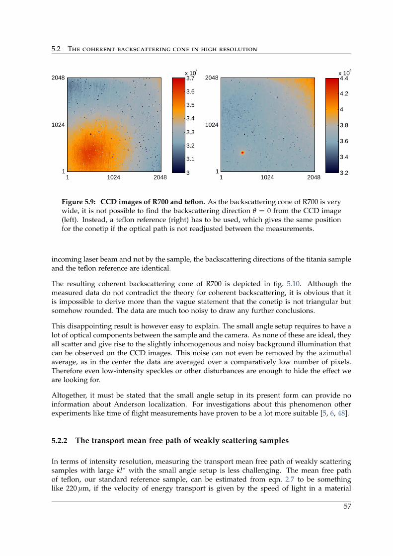
5.2 The coherent backscattering cone in high resolution
1 1024 20481
1024
2048
3
3.1
3.2
3.3
3.4
3.5
3.6
3.7x 10
4
1 1024 20481
1024
2048
3.2
3.4
3.6
3.8
4
4.2
4.4x 10
4
Figure 5.9: CCD images of R700 and teflon. As the backscattering cone of R700 is verywide, it is not possible to find the backscattering direction θ = 0 from the CCD image(left). Instead, a teflon reference (right) has to be used, which gives the same positionfor the conetip if the optical path is not readjusted between the measurements.
incoming laser beam and not by the sample, the backscattering directions of the titania sampleand the teflon reference are identical.
The resulting coherent backscattering cone of R700 is depicted in fig. 5.10. Although themeasured data do not contradict the theory for coherent backscattering, it is obvious that itis impossible to derive more than the vague statement that the conetip is not triangular butsomehow rounded. The data are much too noisy to draw any further conclusions.
This disappointing result is however easy to explain. The small angle setup requires to have alot of optical components between the sample and the camera. As none of these are ideal, theyall scatter and give rise to the slightly inhomogenous and noisy background illumination thatcan be observed on the CCD images. This noise can not even be removed by the azimuthalaverage, as in the center the data are averaged over a comparatively low number of pixels.Therefore even low-intensity speckles or other disturbances are enough to hide the effect weare looking for.
Altogether, it must be stated that the small angle setup in its present form can provide noinformation about Anderson localization. For investigations about this phenomenon otherexperiments like time of flight measurements have proven to be a lot more suitable [5, 6, 48].
5.2.2 The transport mean free path of weakly scattering samples
In terms of intensity resolution, measuring the transport mean free path of weakly scatteringsamples with large kl∗ with the small angle setup is less challenging. The mean free pathof teflon, our standard reference sample, can be estimated from eqn. 2.7 to be somethinglike 220 µm, if the velocity of energy transport is given by the speed of light in a material
57
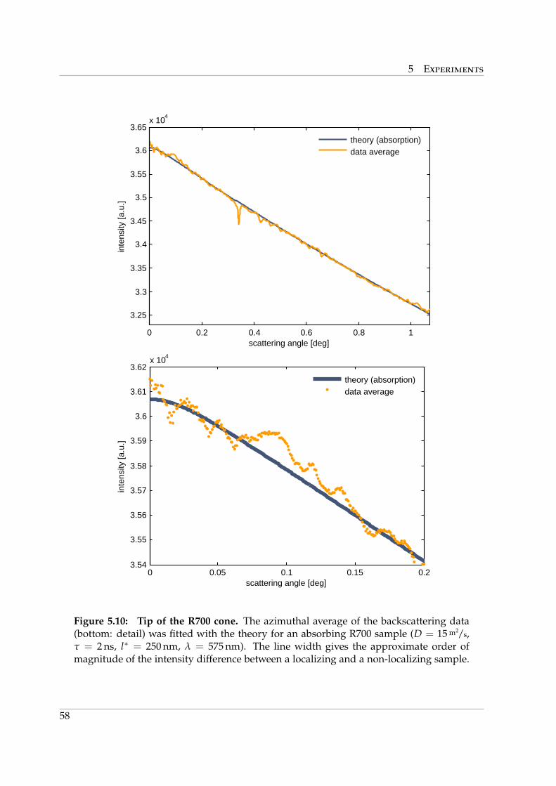
5 Experiments
0 0.2 0.4 0.6 0.8 1
3.25
3.3
3.35
3.4
3.45
3.5
3.55
3.6
3.65x 10
4
scattering angle [deg]
inte
nsity
[a.u
.]
theory (absorption)data average
0 0.05 0.1 0.15 0.23.54
3.55
3.56
3.57
3.58
3.59
3.6
3.61
3.62x 10
4
scattering angle [deg]
inte
nsity
[a.u
.]
theory (absorption)data average
Figure 5.10: Tip of the R700 cone. The azimuthal average of the backscattering data(bottom: detail) was fitted with the theory for an absorbing R700 sample (D = 15 m2/s,τ = 2 ns, l∗ = 250 nm, λ = 575 nm). The line width gives the approximate order ofmagnitude of the intensity difference between a localizing and a non-localizing sample.
58
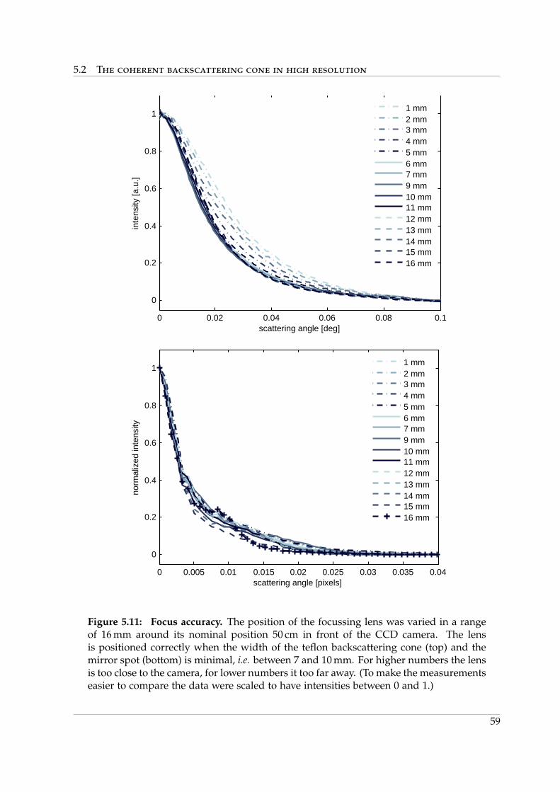
5.2 The coherent backscattering cone in high resolution
0 0.02 0.04 0.06 0.08 0.1
0
0.2
0.4
0.6
0.8
1
scattering angle [deg]
inte
nsity
[a.u
.]
1 mm2 mm3 mm4 mm5 mm6 mm7 mm9 mm10 mm11 mm12 mm13 mm14 mm15 mm16 mm
0 0.005 0.01 0.015 0.02 0.025 0.03 0.035 0.04
0
0.2
0.4
0.6
0.8
1
scattering angle [pixels]
norm
aliz
ed in
tens
ity
1 mm2 mm3 mm4 mm5 mm6 mm7 mm9 mm10 mm11 mm12 mm13 mm14 mm15 mm16 mm
Figure 5.11: Focus accuracy. The position of the focussing lens was varied in a rangeof 16 mm around its nominal position 50 cm in front of the CCD camera. The lensis positioned correctly when the width of the teflon backscattering cone (top) and themirror spot (bottom) is minimal, i.e. between 7 and 10 mm. For higher numbers the lensis too close to the camera, for lower numbers it too far away. (To make the measurementseasier to compare the data were scaled to have intensities between 0 and 1.)
59
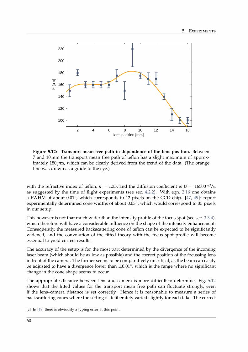
5 Experiments
2 4 6 8 10 12 14 16
100
120
140
160
180
200
220
lens position [mm]
l* [µ
m]
Figure 5.12: Transport mean free path in dependence of the lens position. Between7 and 10 mm the transport mean free path of teflon has a slight maximum of approx-imately 180 µm, which can be clearly derived from the trend of the data. (The orangeline was drawn as a guide to the eye.)
with the refractive index of teflon, n = 1.35, and the diffusion coefficient is D = 16500 m2/s,as suggested by the time of flight experiments (see sec. 4.2.2). With eqn. 2.16 one obtainsa FWHM of about 0.01, which corresponds to 12 pixels on the CCD chip. [47, 49]c reportexperimentally determined cone widths of about 0.03, which would correspond to 35 pixelsin our setup.
This however is not that much wider than the intensity profile of the focus spot (see sec. 3.3.4),which therefore will have a considerable influence on the shape of the intensity enhancement.Consequently, the measured backscattering cone of teflon can be expected to be significantlywidened, and the convolution of the fitted theory with the focus spot profile will becomeessential to yield correct results.
The accuracy of the setup is for the most part determined by the divergence of the incominglaser beam (which should be as low as possible) and the correct position of the focussing lensin front of the camera. The former seems to be comparatively uncritical, as the beam can easilybe adjusted to have a divergence lower than ±0.01, which is the range where no significantchange in the cone shape seems to occur.
The appropriate distance between lens and camera is more difficult to determine. Fig. 5.12shows that the fitted values for the transport mean free path can fluctuate strongly, evenif the lens–camera distance is set correctly. Hence it is reasonable to measure a series ofbackscattering cones where the setting is deliberately varied slightly for each take. The correct
[c] In [49] there is obviously a typing error at this point.
60
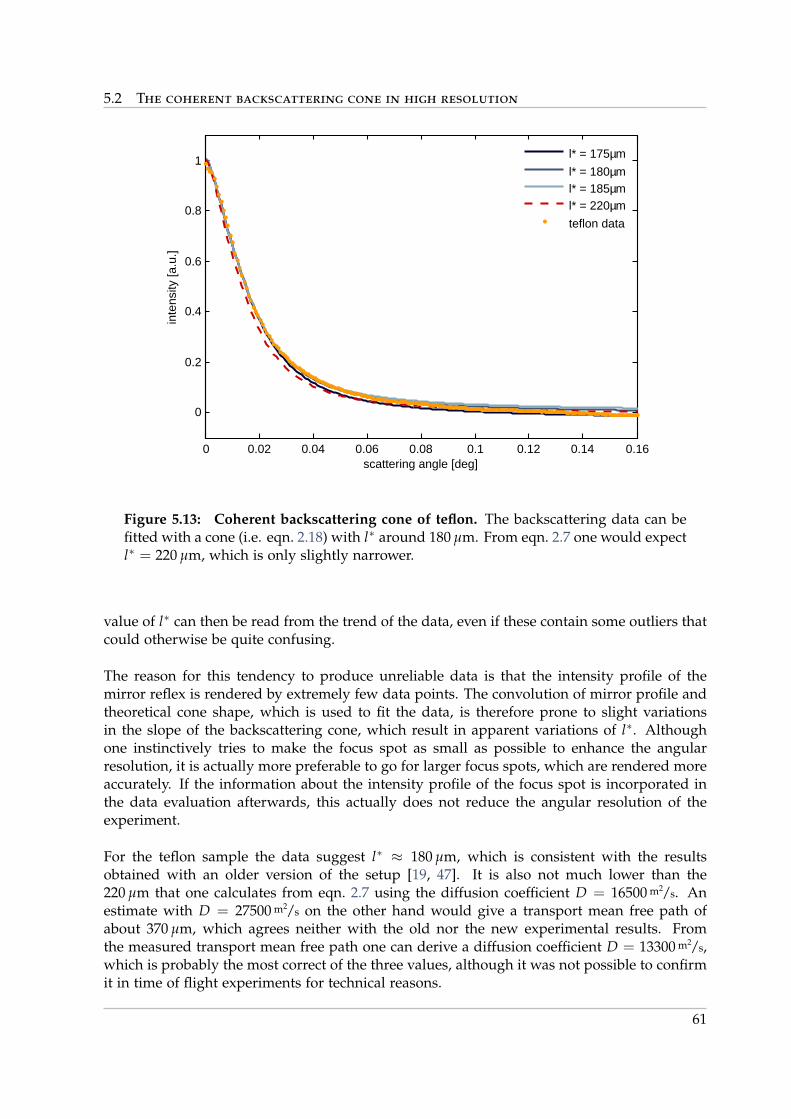
5.2 The coherent backscattering cone in high resolution
0 0.02 0.04 0.06 0.08 0.1 0.12 0.14 0.16
0
0.2
0.4
0.6
0.8
1
scattering angle [deg]
inte
nsity
[a.u
.]
l* = 175µm
l* = 180µml* = 185µml* = 220µm
teflon data
Figure 5.13: Coherent backscattering cone of teflon. The backscattering data can befitted with a cone (i.e. eqn. 2.18) with l∗ around 180 µm. From eqn. 2.7 one would expectl∗ = 220 µm, which is only slightly narrower.
value of l∗ can then be read from the trend of the data, even if these contain some outliers thatcould otherwise be quite confusing.
The reason for this tendency to produce unreliable data is that the intensity profile of themirror reflex is rendered by extremely few data points. The convolution of mirror profile andtheoretical cone shape, which is used to fit the data, is therefore prone to slight variationsin the slope of the backscattering cone, which result in apparent variations of l∗. Althoughone instinctively tries to make the focus spot as small as possible to enhance the angularresolution, it is actually more preferable to go for larger focus spots, which are rendered moreaccurately. If the information about the intensity profile of the focus spot is incorporated inthe data evaluation afterwards, this actually does not reduce the angular resolution of theexperiment.
For the teflon sample the data suggest l∗ ≈ 180 µm, which is consistent with the resultsobtained with an older version of the setup [19, 47]. It is also not much lower than the220 µm that one calculates from eqn. 2.7 using the diffusion coefficient D = 16500 m2/s. Anestimate with D = 27500 m2/s on the other hand would give a transport mean free path ofabout 370 µm, which agrees neither with the old nor the new experimental results. Fromthe measured transport mean free path one can derive a diffusion coefficient D = 13300 m2/s,which is probably the most correct of the three values, although it was not possible to confirmit in time of flight experiments for technical reasons.
61
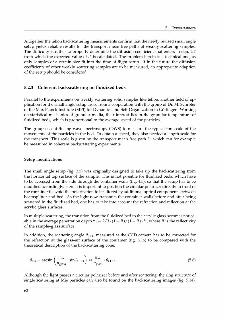
5 Experiments
Altogether the teflon backscattering measurements confirm that the newly revised small anglesetup yields reliable results for the transport mean free paths of weakly scattering samples.The difficulty is rather to properly determine the diffusion coefficient that enters in eqn. 2.7from which the expected value of l∗ is calculated. The problem herein is a technical one, asonly samples of a certain size fit into the time of flight setup. If in the future the diffusioncoefficients of other weakly scattering samples are to be measured, an appropriate adaptionof the setup should be considered.
5.2.3 Coherent backscattering on fluidized beds
Parallel to the experiments on weakly scattering solid samples like teflon, another field of ap-plication for the small angle setup arose from a cooperation with the group of Dr. M. Schroterof the Max Planck Institute (MPI) for Dynamics and Self-Organization in Gottingen. Workingon statistical mechanics of granular media, their interest lies in the granular temperature offluidized beds, which is proportional to the average speed of the particles.
The group uses diffusing wave spectroscopy (DWS) to measure the typical timescale of themovements of the particles in the bed. To obtain a speed, they also needed a length scale forthe transport. This scale is given by the transport mean free path l∗, which can for examplebe measured in coherent backscattering experiments.
Setup modifications
The small angle setup (fig. 3.5) was originally designed to take up the backscattering fromthe horizontal top surface of the sample. This is not possible for fluidized beds, which haveto be accessed from the side through the container walls (fig. 4.5), so that the setup has to bemodified accordingly. Here it is important to position the circular polarizer directly in front ofthe container to avoid the polarization to be altered by additional optical components betweenbeamsplitter and bed. As the light now transmits the container walls before and after beingscattered in the fluidized bed, one has to take into account the refraction and reflection at theacrylic glass surfaces.
In multiple scattering, the transition from the fluidized bed to the acrylic glass becomes notice-able in the average penetration depth z0 = 2/3 · (1+ R)/(1− R) · l∗, where R is the reflectivityof the sample–glass surface.
In addition, the scattering angle θCCD measured at the CCD camera has to be corrected forthe refraction at the glass–air surface of the container (fig. 5.16) to be compared with thetheoretical description of the backscattering cone:
θms = arcsin(
nair
nglass· sin θCCD
)≈ nair
nglass· θCCD (5.8)
Although the light passes a circular polarizer before and after scattering, the ring structure ofsingle scattering at Mie particles can also be found on the backscattering images (fig. 5.14).
62
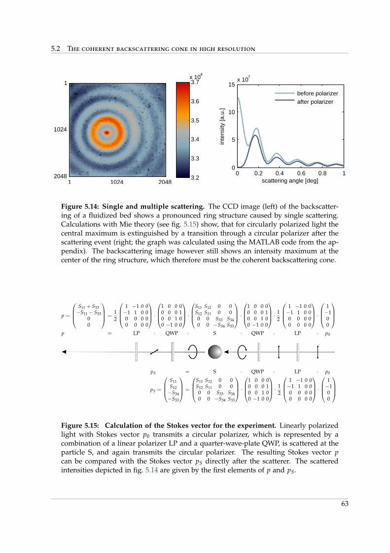
5.2 The coherent backscattering cone in high resolution
1 1024 2048
1
1024
2048 3.2
3.3
3.4
3.5
3.6
3.7x 10
4
0 0.2 0.4 0.6 0.8 10
5
10
15x 10
7
scattering angle [deg]
inte
nsity
[a.u
.]
before polarizerafter polarizer
Figure 5.14: Single and multiple scattering. The CCD image (left) of the backscatter-ing of a fluidized bed shows a pronounced ring structure caused by single scattering.Calculations with Mie theory (see fig. 5.15) show, that for circularly polarized light thecentral maximum is extinguished by a transition through a circular polarizer after thescattering event (right; the graph was calculated using the MATLAB code from the ap-pendix). The backscattering image however still shows an intensity maximum at thecenter of the ring structure, which therefore must be the coherent backscattering cone.
p =
S11 + S33−S11 − S33
00
=12
1 −1 0 0−1 1 0 00 0 0 00 0 0 0
·
1 0 0 00 0 0 10 0 1 00 −1 0 0
·
S11 S12 0 0S12 S11 0 00 0 S33 S340 0 −S34 S33
·
1 0 0 00 0 0 10 0 1 00 −1 0 0
· 12
1 −1 0 0−1 1 0 00 0 0 00 0 0 0
·
1−100
p = LP · QWP · S · QWP · LP · p0
pS = S · QWP · LP · p0
pS =
S11S12−S34−S33
=
S11 S12 0 0S12 S11 0 00 0 S33 S340 0 −S34 S33
·
1 0 0 00 0 0 10 0 1 00 −1 0 0
· 12
1 −1 0 0−1 1 0 00 0 0 00 0 0 0
·
1−100
Figure 5.15: Calculation of the Stokes vector for the experiment. Linearly polarizedlight with Stokes vector p0 transmits a circular polarizer, which is represented by acombination of a linear polarizer LP and a quarter-wave-plate QWP, is scattered at theparticle S, and again transmits the circular polarizer. The resulting Stokes vector pcan be compared with the Stokes vector pS directly after the scatterer. The scatteredintensities depicted in fig. 5.14 are given by the first elements of p and pS.
63
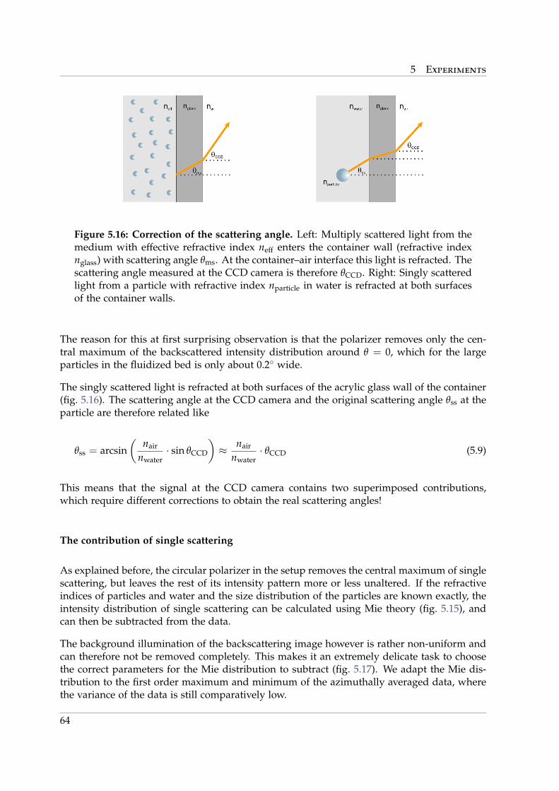
5 Experiments
Figure 5.16: Correction of the scattering angle. Left: Multiply scattered light from themedium with effective refractive index neff enters the container wall (refractive indexnglass) with scattering angle θms. At the container–air interface this light is refracted. Thescattering angle measured at the CCD camera is therefore θCCD. Right: Singly scatteredlight from a particle with refractive index nparticle in water is refracted at both surfacesof the container walls.
The reason for this at first surprising observation is that the polarizer removes only the cen-tral maximum of the backscattered intensity distribution around θ = 0, which for the largeparticles in the fluidized bed is only about 0.2 wide.
The singly scattered light is refracted at both surfaces of the acrylic glass wall of the container(fig. 5.16). The scattering angle at the CCD camera and the original scattering angle θss at theparticle are therefore related like
θss = arcsin(
nair
nwater· sin θCCD
)≈ nair
nwater· θCCD (5.9)
This means that the signal at the CCD camera contains two superimposed contributions,which require different corrections to obtain the real scattering angles!
The contribution of single scattering
As explained before, the circular polarizer in the setup removes the central maximum of singlescattering, but leaves the rest of its intensity pattern more or less unaltered. If the refractiveindices of particles and water and the size distribution of the particles are known exactly, theintensity distribution of single scattering can be calculated using Mie theory (fig. 5.15), andcan then be subtracted from the data.
The background illumination of the backscattering image however is rather non-uniform andcan therefore not be removed completely. This makes it an extremely delicate task to choosethe correct parameters for the Mie distribution to subtract (fig. 5.17). We adapt the Mie dis-tribution to the first order maximum and minimum of the azimuthally averaged data, wherethe variance of the data is still comparatively low.
64
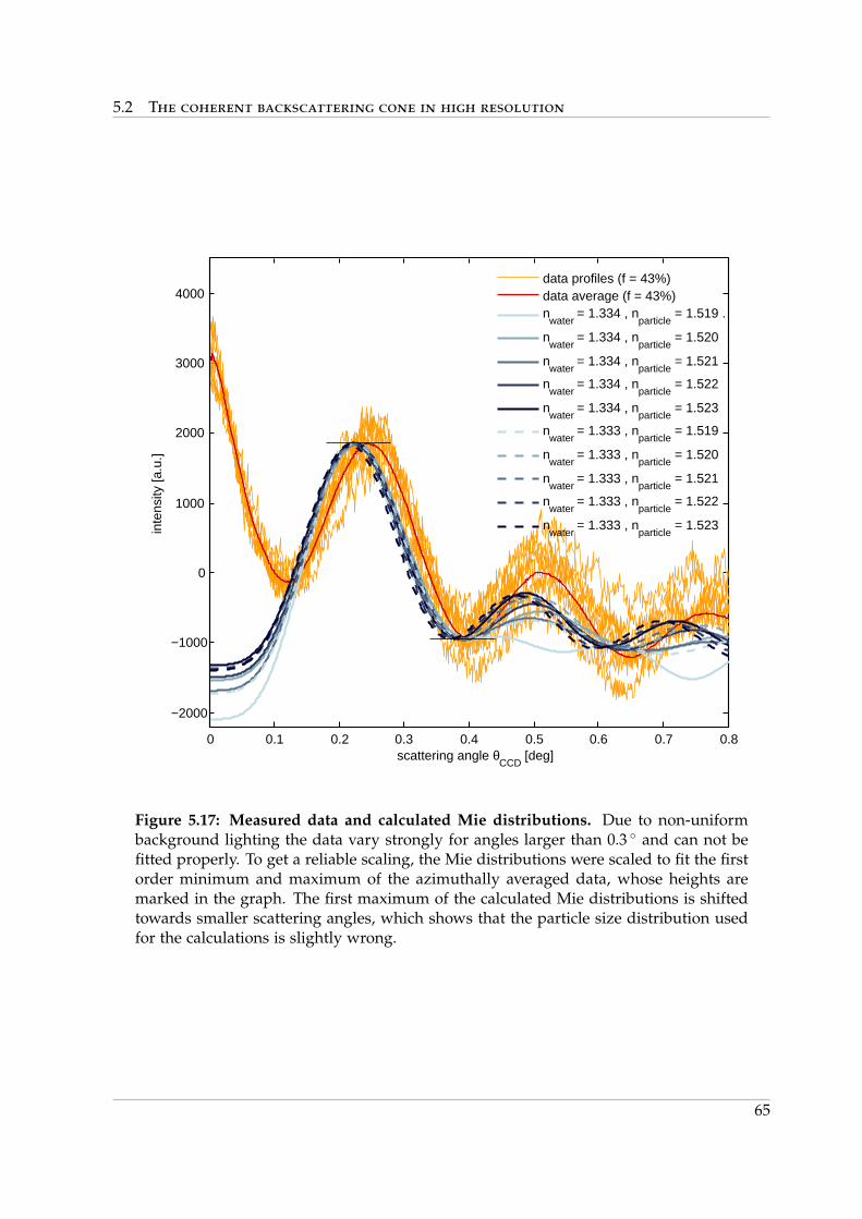
5.2 The coherent backscattering cone in high resolution
0 0.1 0.2 0.3 0.4 0.5 0.6 0.7 0.8
−2000
−1000
0
1000
2000
3000
4000
scattering angle θCCD
[deg]
inte
nsity
[a.u
.]
data profiles (f = 43%)data average (f = 43%)n
water = 1.334 , n
particle = 1.519 .
nwater
= 1.334 , nparticle
= 1.520
nwater
= 1.334 , nparticle
= 1.521
nwater
= 1.334 , nparticle
= 1.522
nwater
= 1.334 , nparticle
= 1.523
nwater
= 1.333 , nparticle
= 1.519
nwater
= 1.333 , nparticle
= 1.520
nwater
= 1.333 , nparticle
= 1.521
nwater
= 1.333 , nparticle
= 1.522
nwater
= 1.333 , nparticle
= 1.523
Figure 5.17: Measured data and calculated Mie distributions. Due to non-uniformbackground lighting the data vary strongly for angles larger than 0.3 and can not befitted properly. To get a reliable scaling, the Mie distributions were scaled to fit the firstorder minimum and maximum of the azimuthally averaged data, whose heights aremarked in the graph. The first maximum of the calculated Mie distributions is shiftedtowards smaller scattering angles, which shows that the particle size distribution usedfor the calculations is slightly wrong.
65
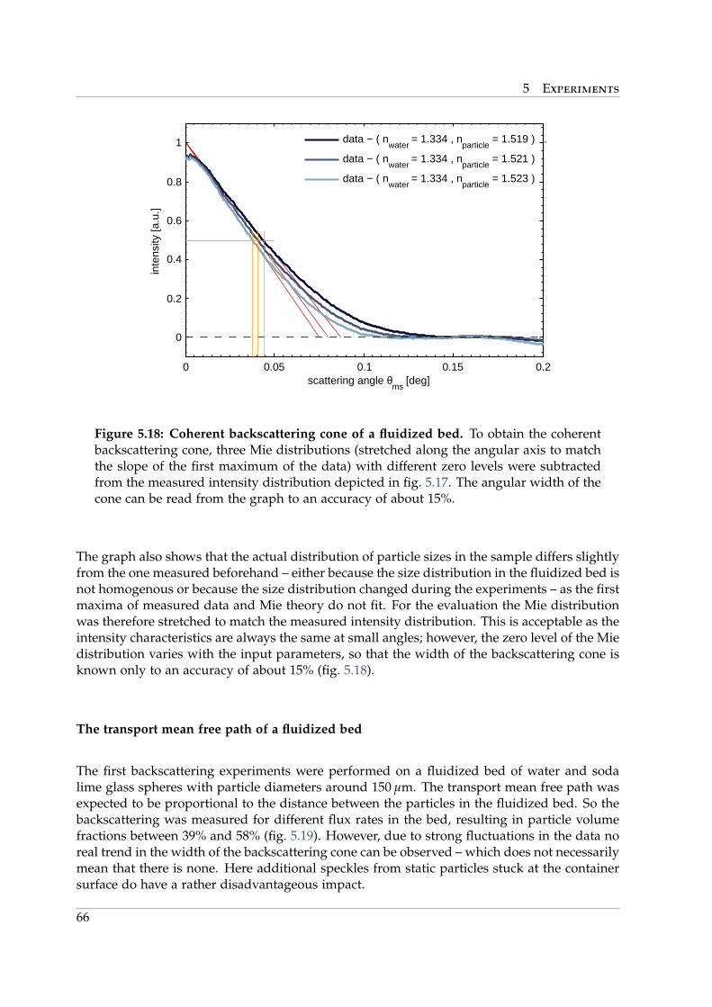
5 Experiments
0 0.05 0.1 0.15 0.2
0
0.2
0.4
0.6
0.8
1
scattering angle θms
[deg]
inte
nsity
[a.u
.]
data − ( n
water = 1.334 , n
particle = 1.519 ) .
data − ( nwater
= 1.334 , nparticle
= 1.521 )
data − ( nwater
= 1.334 , nparticle
= 1.523 )
Figure 5.18: Coherent backscattering cone of a fluidized bed. To obtain the coherentbackscattering cone, three Mie distributions (stretched along the angular axis to matchthe slope of the first maximum of the data) with different zero levels were subtractedfrom the measured intensity distribution depicted in fig. 5.17. The angular width of thecone can be read from the graph to an accuracy of about 15%.
The graph also shows that the actual distribution of particle sizes in the sample differs slightlyfrom the one measured beforehand – either because the size distribution in the fluidized bed isnot homogenous or because the size distribution changed during the experiments – as the firstmaxima of measured data and Mie theory do not fit. For the evaluation the Mie distributionwas therefore stretched to match the measured intensity distribution. This is acceptable as theintensity characteristics are always the same at small angles; however, the zero level of the Miedistribution varies with the input parameters, so that the width of the backscattering cone isknown only to an accuracy of about 15% (fig. 5.18).
The transport mean free path of a fluidized bed
The first backscattering experiments were performed on a fluidized bed of water and sodalime glass spheres with particle diameters around 150 µm. The transport mean free path wasexpected to be proportional to the distance between the particles in the fluidized bed. So thebackscattering was measured for different flux rates in the bed, resulting in particle volumefractions between 39% and 58% (fig. 5.19). However, due to strong fluctuations in the data noreal trend in the width of the backscattering cone can be observed – which does not necessarilymean that there is none. Here additional speckles from static particles stuck at the containersurface do have a rather disadvantageous impact.
66
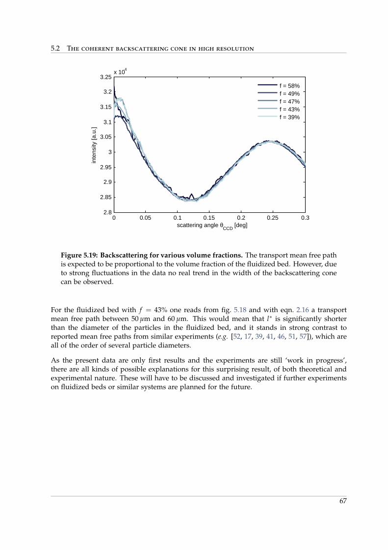
5.2 The coherent backscattering cone in high resolution
0 0.05 0.1 0.15 0.2 0.25 0.32.8
2.85
2.9
2.95
3
3.05
3.1
3.15
3.2
3.25x 10
4
scattering angle θCCD
[deg]
inte
nsity
[a.u
.]
f = 58%f = 49%f = 47%f = 43%f = 39%
Figure 5.19: Backscattering for various volume fractions. The transport mean free pathis expected to be proportional to the volume fraction of the fluidized bed. However, dueto strong fluctuations in the data no real trend in the width of the backscattering conecan be observed.
For the fluidized bed with f = 43% one reads from fig. 5.18 and with eqn. 2.16 a transportmean free path between 50 µm and 60 µm. This would mean that l∗ is significantly shorterthan the diameter of the particles in the fluidized bed, and it stands in strong contrast toreported mean free paths from similar experiments (e.g. [52, 17, 39, 41, 46, 51, 57]), which areall of the order of several particle diameters.
As the present data are only first results and the experiments are still ‘work in progress’,there are all kinds of possible explanations for this surprising result, of both theoretical andexperimental nature. These will have to be discussed and investigated if further experimentson fluidized beds or similar systems are planned for the future.
67

5 Experiments
68
6 Summary
The focus of the work presented in this thesis lay on improvements of the experimental tech-niques for the investigation of multiple scattering phenomena, and in particular the coherentbackscattering cone of visible light.
This interference effect had been found to apparently violate the principle of conservation ofenergy: The total amount of backscattered energy can not exceed the energy which the lightsource inserts into the sample. The intensity enhancement of the cone should therefore be bal-anced by a corresponding intensity cutback, which however had never been observed neitherin experiment nor in theory. Inaccuracies in the latter two being the only possible explana-tion, we reviewed our backscattering experiments and the evaluation of the backscatteringdata, and also tested an improved theory which had been worked out by E. Akkermans andG. Montambaux.
The two theoreticians extended the theoretical description of the backscattering cone by twoadditional terms that contribute to the total backscattered energy in the same order as thecone itself. They lead to a cutback of the scattered intensity below the level of the incoherentaddition of the backscattered intensity which balances the intensity enhancement of the cone.In the new theoretical description of the backscattering cone the energy is therefore conserved.
The key to a precise measurement of the shape of the coherent backscattering cone was thecorrect calibration of the photodiodes of the wide angle setup. For this a teflon referencesample is used, the albedo of which differs from the titania albedo by about 10%. In ear-lier experiments this difference had been neglected, which led to a misrepresentation of thebackscattering cone, so that conservation of energy seemed to be seriously violated. If how-ever the albedos of sample and reference are considered in the evaluation, one can observean intensity cutback at the wings of the cone, which balances the intensity enhancement inbackscattering direction, and which also agrees with the predictions made by Akkermans andMontambaux.
A second part of this work concerned the remodeling of the small angle setup for the measure-ment of the scattered intensity distribution in a small range around backscattering direction.One goal was to detect Anderson localization by the rounding of the tip of the coherentbackscattering cone. For this an older CCD camera was replaced by a high resolving model,which improves the maximum intensity resolution by more than two orders of magnitude andthe maximum angular resolution or respectively the maximum angular range by a factor ofthree. However, it turned out that the optical components between sample and camera causetoo much extraneous light, so that the necessary intensity resolution can not be achieved.
Still, the improved setup can be used to measure the transport mean free path of weaklyscattering samples like for example teflon. For teflon one can measure a cone with FWHM ≈0.03, corresponding to a transport mean free path l∗ = 180 µm and a diffusion coefficient
6 Summary
D = 13300 m2/s. This agrees pretty well with results of measurements with the old setup andwith the results of the wide angle experiments, which yield correct results if the diffusioncoefficient obtained with the small angle setup is used for the evaluation. With these findingsthe reliability of the results of the small angle setup is confirmed.
Another application for the small angle setup was to determine the transport mean free pathof fluidized beds. As the scattering particles in these experiments are rather large and have aregularly spherical shape, the intensity distribution of the backscattered light is superimposedby the ring structure of the single scattering on the Mie particles. This structure can howeverbe calculated theoretically and adapted to the measured curves, so that the backscatteringcone can be extracted from the data.
In first measurements the width of the backscattering cone led to a transport mean free paththat was significantly shorter than the particle diameter of the scatterers. This is in strongcontrast to the results of similar experiments, which are reported to be of the order of severalparticle diameters. The reason for this is still under discussion; however, the basic procedurefor the evaluation of the backscattering data of fluidized beds was tested successfully.
For future experiments, the combination of the two revised backscattering setups offers theunique possibility to measure kl∗ over more than three decades, from samples at the transi-tion to Anderson localization at kl∗ ≈ 1 to weakly scattering samples with extremely narrowbackscattering cones. Possible applications range from experiments on new, custom designedparticles with small kl∗ to measurements on foams or biological tissue. Some of these ex-periments are already planned for the near future, and will hopefully provide a step furthertowards fully understanding multiple scattering.
70
Bibliography
[1] http://www.schneiderkreuznach.com/industrial filters/polarization filters.htms,17.02.2010.
[2] Matlab. The MathWorks Inc., 2007.
[3] MiePlot. [email protected], 2008.
[4] http://www.lenntech.com/teflon.htm, 2.11.2009.
[5] C. M. Aegerter, M. Storzer, W. Buhrer, S. Fiebig, and G. Maret, Experimental sig-natures of Anderson localization of light in three dimensions, Journal of Modern Optics, 54(2007), p. 2667.
[6] C. M. Aegerter, M. Storzer, S. Fiebig, W. Buhrer, and G. Maret, Observation of An-derson localization of light in three dimensions, Journal of the Optical Society of America A,24 (2007), p. A23.
[7] C. M. Aegerter, M. Storzer, and G. Maret, Experimental determination of critical expo-nents in Anderson localisation of light, Europhysics Letters, 75 (2006), p. 562.
[8] E. Akkermans and G. Montambaux, Coherent effects in the multiple scattering of lightin random media, in Wave Scattering in Complex Media: From Theory to Applications,B. van Tiggelen and S. Skipetrov, eds., Kluwer Academic Publishers, 2003.
[9] , Memo on cbs and conservation of energy. Private communication, May 2007.
[10] , Mesoscopic Physics of Electrons and Photons, Cambridge University Press, 2007. ISBN978-0-521-85512-9.
[11] E. Akkermans, P. E. Wolf, and R. Maynard, Coherent backscattering of light by disorderedmedia: Analysis of the peak line shape, Physical Review Letters, 56 (1986), p. 1471.
[12] E. Akkermans, P. E. Wolf, R. Maynard, and G. Maret, Theoretical study of the coherentbackscattering of light by disordered media, Journal de Physique France, 49 (1988), p. 77.
[13] P. W. Anderson, Absence of diffusion in certain random lattices, Physical Review, 109 (1958),p. 1492.
[14] , The question of classical localization - a theory of white paint, Philosophical MagazineB, 52 (1985), p. 505.
[15] G. Bayer and T. Niederdrank, Weak localization of acoustic waves in strongly scatteringmedia, Physical Review Letters, 70 (1993), p. 3884.
[16] C. F. Bohren and D. R. Huffman, Absorption and Scattering of Light by Small Particles,Wiley-Interscience, 1998. ISBN 0-471-29340-7.
Bibliography
[17] J. Crassous, Diffusive wave spectroscopy of a random close packing of spheres, The EuropeanPhysical Journal E, 23 (2007), p. 145.
[18] R. Dalichaouch, J. P. Armstrong, S. Schultz, P. M. Platzman, and S. L. McCall,Microwave localization by two-dimensional random scattering.pdf, Nature, 354 (1991), p. 53.
[19] S. Fiebig, C. M. Aegerter, W. Buhrer, M. Storzer, E. Akkermans, G. Montambaux,and G. Maret, Conservation of energy in coherent backscattering of light, Europhysics Let-ters, 81 (2008), p. 64004.
[20] S. Fraden and G. Maret, Multiple scattering of light from concentrated interacting suspen-sion, Physical Review Letters, 65 (1990), p. 512.
[21] J. C. M. Garnett, Colours in metal glasses and in metallic films, Philosophical Transactionsof the Royal Society of London. Series A, 203 (1904), p. 385.
[22] P. Gross, Coherent backscattering close to the transition to strong localization of light, diplomathesis, Universitat Konstanz, 2005.
[23] P. Gross, M. Storzer, S. Fiebig, M. Clausen, G. Maret, and C. M. Aegerter, A precisemethod to determine the angular distribution of backscattered light to high angles, Review ofScientific Instruments, 78 (2007), p. 033105.
[24] B. W. Hapke, R. M. Nelson, and W. D. Smythe, The opposition effect of the moon: Thecontribution of coherent backscatter.pdf, Science, 260 (1993), p. 509.
[25] S. Hikami, Anderson localization in a nonlinear-sigma-model representation, Physical ReviewB, 24 (1981), p. 2671.
[26] H. Hinrichsen and D. E. Wolf, eds., The Physics of Granular Media, Wiley-VCH Verlag,2004. ISBN 3-527-40373-6.
[27] A. F. Ioffe and A. R. Regel, Non-crystalline, amorphous and liquid electronic semiconductors,Prog. Semicond., 4 (1960), p. 237.
[28] S. John, Electromagnetic absorption in a disordered medium near a photon mobility edge, Phys-ical Review Letters, 53 (1984), p. 2169.
[29] M. Kaveh, M. Rosenbluh, I. Edrei, and I. Freund, Weak localization and light scatteringfrom disordered solids, Physical Review Letters, 57 (1986), p. 2049.
[30] D. S. Kliger, J. W. Lewis, and C. E. Randall, Polarized Light in Optics and Spectroscopy,Academic Press, Inc, 1990. ISBN 0-12-414975-8.
[31] Y. Kuga and A. Ishimaru, Retroreflectance from a dense distribution of spherical particles,Journal of the Optical Society of America A, 1 (1984), p. 831.
[32] V. L. Kuzmin and I. V. Meglinski, Numerical simulation of coherent backscattering andtemporal intensity correlations in random media, Quantum Electronics, 36 (2006), p. 990.
[33] J. H. Lambert, Photometria sive de mensure et gradibus luminis colorum et umbra, Klett, 1760.Review in: Gottingische Gelehrte Anzeigen, 118. Stuck den 2. October 1760, p. 1010.
72
Bibliography
[34] E. Larose, L. Margerin, B. A. van Tiggelen, and M. Campillo, Weak localization ofseismic waves, Physical Review Letters, 93 (2004), p. 048501.
[35] R. Lenke, R. Lehner, and G. Maret, Magnetic-field effects on coherent backscattering oflight in case of mie spheres, Europhysics Letters, 52 (2000), p. 620.
[36] R. Lenke and G. Maret, Affecting weak light localization by strong magnetic fields, PhysicaScripta, T49 (1993), p. 605.
[37] , Magnetic field effects on coherent backscattering of light, European Physical Journal B,17 (2000), p. 171.
[38] , Multiple scattering of light: Coherent backscattering and transmission, in Scattering inPolymeric and Colloidal Systems, W. Brown and K. Mortensen, eds., Gordon and BreachScience Publishers, 2000.
[39] E. Leutz and J. Ricka, On light propagation through glass bead packings, Optics Communi-cations, 126 (1996), p. 260.
[40] G. Maret, Recent experiments on multiple scattering and localization of light, in Les Houches,Session LXI, 1994: Physique Quantique Mesoscopique – Mesocopic Quantum Physics,E. Akkermans, G. Montamaux, J.-L. Pichard, and J. Zinn-Justion, eds., Elsevier ScienceB. V., 1995.
[41] N. Menon and D. J. Durian, Diffusing-wave spectroscopy of dynamics in a three-dimensionalgranular flow, Science, 275 (1997), p. 1920.
[42] G. Mie, Beitrage zur Optik truber Medien, speziell kolloidaler Metallosungen, Annalen derPhysik, 330 (1908), p. 377.
[43] H. Mueller, The foundation of optics, Journal of the Optical Society of America, 38 (1948),p. 661.
[44] D. Pine, D. Weitz, P. Chaikin, and E. Herbolzheimer, Diffusing-wave spectroscopy,Physical Review Letters, 60 (1988), p. 1134.
[45] S. E. Skipetrov and B. A. van Tiggelen, Dynamics of weakly localized waves, PhysicalReview Letters, 92 (2004), p. 113901.
[46] P. Snabre and J. Crassous, Multispeckle diffusing wave spectroscopy of colloidal particlessuspended in a random packing of glass spheres, The European Physical Journal E, 29 (2009),p. 149.
[47] M. Storzer, Anderson Localization of Light, PhD thesis, Universitat Konstanz, 2006.
[48] M. Storzer, P. Gross, C. M. Aegerter, and G. Maret, Observation of the critical regimenear Anderson localization of light, Physical Review Letters, 96 (2006), p. 063904.
[49] R. Tweer, Vielfachstreuung von Licht in Systemen dicht gepackter Mie-Streuer: Auf dem Wegzur Anderson-Lokaliserung?, PhD thesis, Universitat Konstanz, 2002.
[50] S. Utermann, August 2009. Private communication.
73
Bibliography
[51] , Getting the hang of diffusive light scattering: measuring l* by transmission. Privatecommunication, August 2009.
[52] M. P. van Albada and A. Lagendijk, Observation of weak localization of light in a randommedia, Physical Review Letters, 55 (1985), p. 2696.
[53] H. C. van de Hulst, Accurate eigenvalues and exact extrapolation lengths in radiative transfer,Astronomy and Astrophysics, 235 (1990), p. 511.
[54] M. van Rossum and T. M. Nieuwenhuizen, Multiple scattering of classical waves - mi-croscopy, mesoscopy, and diffusion, Reviews of Modern Physics, 71 (1999), p. 313.
[55] D. S. Wiersma, An accurate technique to record the angular distribution of backscattered light,Review of Scientific Instruments, 66 (1995), p. 5473.
[56] , Light in strongly scattering and amplifying random media, PhD thesis, Universiteit vanAmsterdam, 1995.
[57] P. E. Wolf and G. Maret, Weak lokalization and coherent backscattering of photons in disor-dered media, Physical Review Letters, 55 (1985), p. 2696.
[58] J. X. Zhu, D. J. Pine, and D. A. Weitz, Internal reflection of diffusive light in random media,Physical Review A, 44 (1991), p. 3948.
74

Figures and Tables
Figures
Backscattering of a fluidized bed . . . . . . . . . . . . . . . . . . . . . . . . . . . . . . Title
2.1 Coordinate system of single scattering . . . . . . . . . . . . . . . . . . . . . . . . 5
2.2 Vibration ellipse . . . . . . . . . . . . . . . . . . . . . . . . . . . . . . . . . . . . . 7
2.3 Polarization of a scattered wave . . . . . . . . . . . . . . . . . . . . . . . . . . . . 8
2.4 Scattering cross section and scattering anisotropy . . . . . . . . . . . . . . . . . 9
2.5 Random walk . . . . . . . . . . . . . . . . . . . . . . . . . . . . . . . . . . . . . . 10
2.6 Scattering in the presence of a single boundary . . . . . . . . . . . . . . . . . . 12
2.7 Scattering in the presence of two parallel boundaries . . . . . . . . . . . . . . . 13
2.8 Radiative transfer . . . . . . . . . . . . . . . . . . . . . . . . . . . . . . . . . . . . 14
2.9 Photon flux in backscattering geometry . . . . . . . . . . . . . . . . . . . . . . . 16
2.10 Speckles . . . . . . . . . . . . . . . . . . . . . . . . . . . . . . . . . . . . . . . . . 18
2.11 Theorem of reciprocity . . . . . . . . . . . . . . . . . . . . . . . . . . . . . . . . . 19
2.12 Diffuson and cooperon . . . . . . . . . . . . . . . . . . . . . . . . . . . . . . . . . 21
2.13 Coherent backscattering with absorption . . . . . . . . . . . . . . . . . . . . . . 22
2.14 Coherent backscattering with absorption – unnormalized cooperon . . . . . . . 23
3.1 Laser system . . . . . . . . . . . . . . . . . . . . . . . . . . . . . . . . . . . . . . . 25
3.2 Wide angle setup . . . . . . . . . . . . . . . . . . . . . . . . . . . . . . . . . . . . 26
3.3 Polarizer effectiveness . . . . . . . . . . . . . . . . . . . . . . . . . . . . . . . . . 27
3.4 Conetip rounding from absorption and localization . . . . . . . . . . . . . . . . 29
3.5 Small angle setup . . . . . . . . . . . . . . . . . . . . . . . . . . . . . . . . . . . . 30
3.6 The optical setup . . . . . . . . . . . . . . . . . . . . . . . . . . . . . . . . . . . . 31
3.7 Sample shaker . . . . . . . . . . . . . . . . . . . . . . . . . . . . . . . . . . . . . . 32

Figures and Tables
3.8 Time of flight setup . . . . . . . . . . . . . . . . . . . . . . . . . . . . . . . . . . . 33
4.1 Particle size and polydispersity . . . . . . . . . . . . . . . . . . . . . . . . . . . . 36
4.2 Refractive index . . . . . . . . . . . . . . . . . . . . . . . . . . . . . . . . . . . . . 37
4.3 Reflectivity . . . . . . . . . . . . . . . . . . . . . . . . . . . . . . . . . . . . . . . . 38
4.4 Titania and teflon samples . . . . . . . . . . . . . . . . . . . . . . . . . . . . . . . 40
4.5 Fluidized bed . . . . . . . . . . . . . . . . . . . . . . . . . . . . . . . . . . . . . . 41
4.6 Particle size distribution in the fluidized bed . . . . . . . . . . . . . . . . . . . . 42
5.1 Calibration . . . . . . . . . . . . . . . . . . . . . . . . . . . . . . . . . . . . . . . . 44
5.2 Comparison of the albedos . . . . . . . . . . . . . . . . . . . . . . . . . . . . . . 46
5.3 Calculated photon density distributions in the Teflon sample . . . . . . . . . . 47
5.4 Contributions to the cooperon . . . . . . . . . . . . . . . . . . . . . . . . . . . . . 50
5.5 Old and new theory . . . . . . . . . . . . . . . . . . . . . . . . . . . . . . . . . . 51
5.6 Distribution of backscattered energies. . . . . . . . . . . . . . . . . . . . . . . . . 53
5.7 Example wide angle backscattering data . . . . . . . . . . . . . . . . . . . . . . 54
5.8 Distribution of backscattered energies . . . . . . . . . . . . . . . . . . . . . . . . 55
5.9 CCD images of R700 and teflon . . . . . . . . . . . . . . . . . . . . . . . . . . . . 57
5.10 Tip of the R700 cone . . . . . . . . . . . . . . . . . . . . . . . . . . . . . . . . . . 58
5.11 Focus accuracy . . . . . . . . . . . . . . . . . . . . . . . . . . . . . . . . . . . . . 59
5.12 Transport mean free path in dependence of the lens position . . . . . . . . . . . 60
5.13 Coherent backscattering cone of teflon . . . . . . . . . . . . . . . . . . . . . . . . 61
5.14 Single and multiple scattering . . . . . . . . . . . . . . . . . . . . . . . . . . . . . 63
5.15 Calculation of the Stokes vector for the experiment . . . . . . . . . . . . . . . . 63
5.16 Correction of the scattering angle . . . . . . . . . . . . . . . . . . . . . . . . . . . 64
5.17 Measured data and Mie distributions . . . . . . . . . . . . . . . . . . . . . . . . 65
5.18 Coherent backscattering cone of a fluidized bed . . . . . . . . . . . . . . . . . . 66
5.19 Backscattering for various volume fractions . . . . . . . . . . . . . . . . . . . . . 67
76

Figures and Tables
Tables
4.1 Colloidal samples . . . . . . . . . . . . . . . . . . . . . . . . . . . . . . . . . . . . 39
5.1 Albedos . . . . . . . . . . . . . . . . . . . . . . . . . . . . . . . . . . . . . . . . . . 49
77

Figures and Tables
78
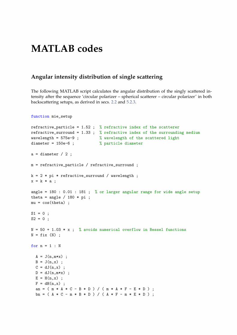
MATLAB codes
Angular intensity distribution of single scattering
The following MATLAB script calculates the angular distribution of the singly scattered in-tensity after the sequence ‘circular polarizer – spherical scatterer – circular polarizer’ in bothbackscattering setups, as derived in secs. 2.2 and 5.2.3.
function mie_setup
refractive_particle = 1.52 ; % refractive index of the scatterer
refractive_surround = 1.33 ; % refractive index of the surrounding medium
wavelength = 575e-9 ; % wavelength of the scattered light
diameter = 150e-6 ; % particle diameter
a = diameter / 2 ;
m = refractive_particle / refractive_surround ;
k = 2 * pi * refractive_surround / wavelength ;
x = k * a ;
angle = 180 : 0.01 : 181 ; % or larger angular range for wide angle setup
theta = angle / 180 * pi ;
mu = cos(theta) ;
S1 = 0 ;
S2 = 0 ;
N = 50 + 1.03 * x ; % avoids numerical overflow in Bessel functions
N = fix (N) ;
for n = 1 : N
A = J(n,m*x) ;
B = J(n,x) ;
C = dJ(n,x) ;
D = dJ(n,m*x) ;
E = H(n,x) ;
F = dH(n,x) ;
an = ( m * A * C - B * D ) / ( m * A * F - E * D ) ;
bn = ( A * C - m * B * D ) / ( A * F - m * E * D ) ;
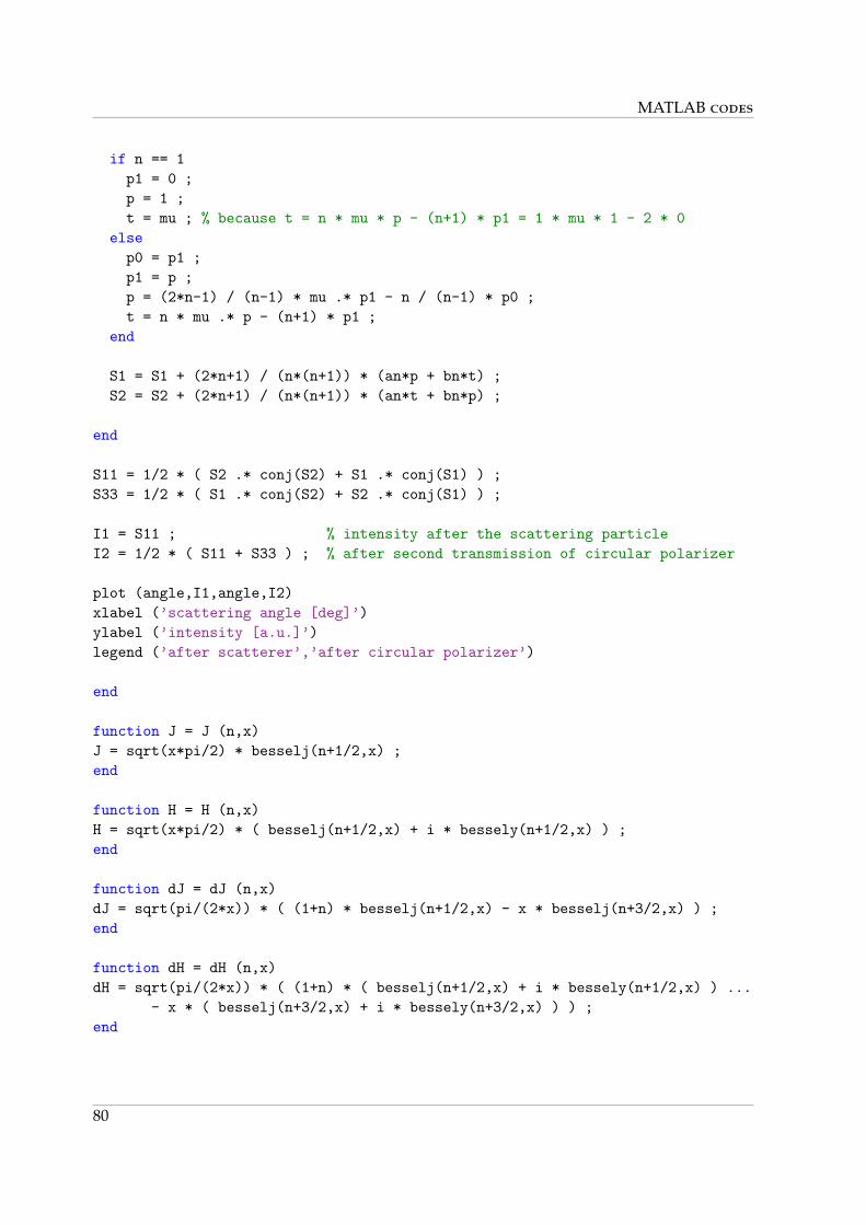
MATLAB codes
if n == 1
p1 = 0 ;
p = 1 ;
t = mu ; % because t = n * mu * p - (n+1) * p1 = 1 * mu * 1 - 2 * 0
else
p0 = p1 ;
p1 = p ;
p = (2*n-1) / (n-1) * mu .* p1 - n / (n-1) * p0 ;
t = n * mu .* p - (n+1) * p1 ;
end
S1 = S1 + (2*n+1) / (n*(n+1)) * (an*p + bn*t) ;
S2 = S2 + (2*n+1) / (n*(n+1)) * (an*t + bn*p) ;
end
S11 = 1/2 * ( S2 .* conj(S2) + S1 .* conj(S1) ) ;
S33 = 1/2 * ( S1 .* conj(S2) + S2 .* conj(S1) ) ;
I1 = S11 ; % intensity after the scattering particle
I2 = 1/2 * ( S11 + S33 ) ; % after second transmission of circular polarizer
plot (angle,I1,angle,I2)
xlabel (’scattering angle [deg]’)
ylabel (’intensity [a.u.]’)
legend (’after scatterer’,’after circular polarizer’)
end
function J = J (n,x)
J = sqrt(x*pi/2) * besselj(n+1/2,x) ;
end
function H = H (n,x)
H = sqrt(x*pi/2) * ( besselj(n+1/2,x) + i * bessely(n+1/2,x) ) ;
end
function dJ = dJ (n,x)
dJ = sqrt(pi/(2*x)) * ( (1+n) * besselj(n+1/2,x) - x * besselj(n+3/2,x) ) ;
end
function dH = dH (n,x)
dH = sqrt(pi/(2*x)) * ( (1+n) * ( besselj(n+1/2,x) + i * bessely(n+1/2,x) ) ...
- x * ( besselj(n+3/2,x) + i * bessely(n+3/2,x) ) ) ;
end
80
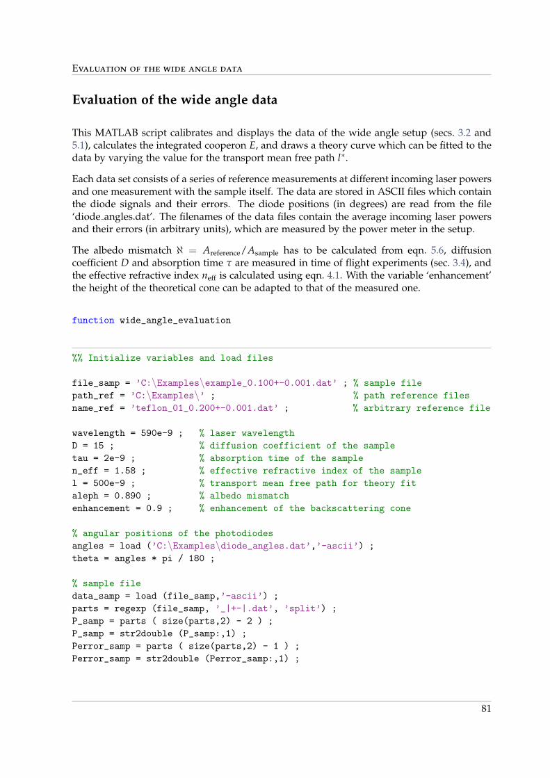
Evaluation of the wide angle data
Evaluation of the wide angle data
This MATLAB script calibrates and displays the data of the wide angle setup (secs. 3.2 and5.1), calculates the integrated cooperon E, and draws a theory curve which can be fitted to thedata by varying the value for the transport mean free path l∗.
Each data set consists of a series of reference measurements at different incoming laser powersand one measurement with the sample itself. The data are stored in ASCII files which containthe diode signals and their errors. The diode positions (in degrees) are read from the file‘diode angles.dat’. The filenames of the data files contain the average incoming laser powersand their errors (in arbitrary units), which are measured by the power meter in the setup.
The albedo mismatch ℵ = Areference/Asample has to be calculated from eqn. 5.6, diffusioncoefficient D and absorption time τ are measured in time of flight experiments (sec. 3.4), andthe effective refractive index neff is calculated using eqn. 4.1. With the variable ‘enhancement’the height of the theoretical cone can be adapted to that of the measured one.
function wide_angle_evaluation
%% Initialize variables and load files
file_samp = ’C:\Examples\example_0.100+-0.001.dat’ ; % sample file
path_ref = ’C:\Examples\’ ; % path reference files
name_ref = ’teflon_01_0.200+-0.001.dat’ ; % arbitrary reference file
wavelength = 590e-9 ; % laser wavelength
D = 15 ; % diffusion coefficient of the sample
tau = 2e-9 ; % absorption time of the sample
n_eff = 1.58 ; % effective refractive index of the sample
l = 500e-9 ; % transport mean free path for theory fit
aleph = 0.890 ; % albedo mismatch
enhancement = 0.9 ; % enhancement of the backscattering cone
% angular positions of the photodiodes
angles = load (’C:\Examples\diode_angles.dat’,’-ascii’) ;
theta = angles * pi / 180 ;
% sample file
data_samp = load (file_samp,’-ascii’) ;
parts = regexp (file_samp, ’_|+-|.dat’, ’split’) ;
P_samp = parts ( size(parts,2) - 2 ) ;
P_samp = str2double (P_samp:,1) ;
Perror_samp = parts ( size(parts,2) - 1 ) ;
Perror_samp = str2double (Perror_samp:,1) ;
81
MATLAB codes
% reference files
index = regexp (name_ref, ’_’, ’start’) ;
index = index (length(index) - 1) ;
namebase = name_ref (1 : index) ;
list = dir ([path_ref,namebase,’*.dat’]) ;
data_ref = zeros (size(list,1),256,2) ;
P_ref = zeros (size(list,1),1) ;
for N = 1 : size(list,1)
filename = [path,list(N).name] ;
data_ref(N,:,:) = load (filename,’-ascii’) ;
parts = regexp (list(N).name, ’_|+-|.dat’, ’split’) ;
p_ref = parts ( size(parts,2) - 2 ) ;
P_ref(N) = str2double (p_ref:,1) ;
end
% other data
k = 2 * pi / wavelength ;
c = 3e8 ; % speed of light
l_approx = D * n_eff / c ;
n_surr = 1 ; % refractive index of surrounding medium = air
R = reflectivity (n_eff,n_surr) ;
%% Calibrate data
cone = zeros(256,1) ;
cone_delta = zeros(256,1) ;
for n = 1 : 256
x = data_ref(:,n) ;
y = P_ref * diffuson(theta(n),l_approx,R) ;
temp1 = sortrows ([x,y],1) ; % sort by x
x = temp1(:,1) ;
y = temp1(:,2) ;
warning off % many warnings because of defect photodiodes (causing NANs)!
[p,s,mu] = polyfit (x,y,3) ;
[cone(n),cone_delta(n)] = polyval (p,data_samp(n),s,mu) ;
warning on
end
%% Fold data
dummy = sortrows ([abs(theta), cone, cone_delta]) ;
theta = dummy (:,1) ;
cone = dummy (:,2) ;
cone_delta = dummy (:,3) ;
82
Evaluation of the wide angle data
% remove NANs and data with huge errors from damaged photodiodes
m = 1 ;
for n = 1 : 256
if isnan (cone(n))
elseif cone_delta(n) > 0.1*P_samp
else
Cone(m) = cone(n) ;
Delta(m) = cone_delta(n) ;
Theta(m) = theta(n) ;
m = m + 1 ;
end
end
cone = Cone ;
cone_delta = Delta ;
theta = Theta ;
clear Theta Cone Delta
% fold data (i.e. -pi/2 < theta < pi/2 -> 0 < theta < pi/2)
m = 1 ;
n = 1 ;
while n < size(theta,2)
if theta(n+1) > theta(n)
Theta(m) = theta(n) ;
Theta(m+1) = theta(n+1) ;
Cone(m) = cone(n) ;
Cone(m+1) = cone(n+1) ;
Delta(m) = cone_delta(n) ;
Delta(m+1) = cone_delta(n+1) ;
n = n + 1 ;
else % theta(n) == theta(n+1)
Theta(m) = theta(n) ;
Cone(m) = (cone(n) + cone(n+1)) / 2 ;
Delta(m) = 0.5 * sqrt ( (cone_delta(n)).^2 + (cone_delta(n+1)).^2 ) ;
n = n + 2 ;
end
m = m + 1 ;
end
cone = Cone ;
cone_delta = Delta ;
theta = Theta ;
%% Derive experimental and theoretical cones
% Correct cone with albedo mismatch
corr_cone = aleph * cone ;
corr_cone_delta = aleph * cone_delta ;
83
MATLAB codes
% Derive experimental diffuson and cooperon
exp_diffuson = diffuson (theta,l,R) * P_samp ;
exp_diffuson_delta = diffuson (theta,l,R) * Perror_samp ;
exp_cooperon = (corr_cone - exp_diffuson) / P_samp ;
exp_cooperon_delta = ...
sqrt ( (corr_cone_delta / P_samp).^2 ...
+ (exp_diffuson_delta / P_samp).^2 ...
+ ((corr_cone - exp_diffuson) / P_samp^2 * Perror_samp).^2 ) ;
% Calculate theory curve
theory_theta = 0 : 0.001*pi : pi/2 ;
theory_cooperon = enhancement * cooperon (theory_theta,k,l,R,D,tau) ;
%% Calculate energy
e_theta = [ 0 , theta , pi/2 ] ;
e_cooperon = [ 1 , exp_cooperon , 0 ] ;
e_cooperon_delta = [ 0 , exp_cooperon_delta , 0 ] ;
E = 2*pi ...
* sum ( ( e_theta(:,2:end) - e_theta(:,1:end-1) ) ...
* 1/2 .* ( e_cooperon(:,1:end-1) .* sin(e_theta(:,1:end-1)) ...
+ e_cooperon(:,2:end) .* sin(e_theta(:,2:end)) ) ) ;
E_delta = 2*pi ...
* sqrt ( sum ( ( 1/2 * ( e_theta(1,2:end) - e_theta(1,1:end-1) ) ...
.* e_cooperon_delta(1:end-1) ).^2 ...
.* sin (1/2 * ( e_theta(1,2:end) + e_theta(1,1:end-1) )) ...
+ ( 1/2 * ( e_theta(1,2:end) - e_theta(1,1:end-1) ) ...
.* e_cooperon_delta(2:end) ).^2 ...
.* sin (1/2 * ( e_theta(1,2:end) + e_theta(1,1:end-1) )) ) ) ;
disp ([’E = ’,num2str(E),’+-’,num2str(E_delta)])
%% Plot data
angles = theta / pi * 180 ;
theory_angles = theory_theta / pi * 180 ;
plot ( angles, exp_cooperon, ’b’, ...
theory_angles, theory_cooperon, ’r’, ...
angles, exp_cooperon+exp_cooperon_delta, ’:b’, ...
angles, exp_cooperon-exp_cooperon_delta, ’:b’ )
xlabel (’scattering angle [deg]’)
ylabel (’cooperon’)
legend (’backscattering data’,’theory’)
end
84
Evaluation of the wide angle data
function d = diffuson (theta,l,R)
z0 = 2/3 * l * (1 + R) / (1 - R) ;
mu = cos(theta) ;
d = ( mu .* (z0/l + mu./(mu+1)) ) ./ (z0/l + 1/2) ;
end
function c = cooperon (theta,k,l,R,D,tau)
z0 = 2/3 * l * (1 + R) / (1 - R) ;
mu = cos(theta) ;
q = k * sin(theta) ;
L_a = sqrt (D * tau) ;
q_a = sqrt (q.^2 + 1/(D*tau)) ;
c = ( l * (l + L_a)^2 * ( (1 - exp(-2*q_a*z0)) ./ ...
(q_a*l) + 2*mu ./ (mu+1) ) ) ...
./ ( L_a^2 * ( l + (1 - exp(-2*z0/L_a)) * L_a ) * ...
( l*q_a + (mu+1) ./ (2*mu) ).^2 ) ;
c_add = (8 * pi * a(k,l,R)) / (3 * k^2 * l * (l + 2 * z0)) * mu ./ (mu + 1) ;
c = c - c_add ;
end
function a = a (k,l,R)
theta = 0.00001*pi : 0.00001*pi : pi/2 ;
z0 = 2/3 * l * (1 + R) / (1 - R) ;
mu = cos(theta) ;
q = k * abs(sin(theta)) ;
E_A = trapz ( theta, ...
3/(8*pi) * 1./(q*l + (mu+1)./(2*mu)).^2 ...
.* ( (1 - exp(-2*q*z0))./(q*l) + (2*mu)./(mu+1) ) ...
.* sin(theta) ) ;
E_BC = trapz ( theta, ...
1/(k*l)^2 * mu./(mu+1) ...
.* sin(theta) ) ;
a = E_A / E_BC ;
end
85
MATLAB codes
function R = reflectivity (n1,n2)
if n1 > n2
theta_totalreflection = asin (n2/n1) ;
else
theta_totalreflection = pi/2 ;
end
theta1 = 0 : pi/100 : theta_totalreflection ;
theta2 = theta_totalreflection+pi/100 : pi/100 : pi/2 ;
theta = [ theta1, theta2 ] ;
R_parallel = ( n1 * cos(theta1) ...
- n2 * sqrt( 1 - (n1 / n2 * sin(theta1)).^2 ) ).^2 ./ ...
( n1 * cos(theta1) ...
+ n2 * sqrt( 1 - (n1 / n2 * sin(theta1)).^2 ) ).^2 ;
R_parallel = [ R_parallel , ones(size(theta2)) ] ;
R_perp = ( n1 * sqrt( 1 - (n1 / n2 * sin(theta1)).^2 ) ...
- n2 * cos(theta1) ).^2 ./ ...
( n1 * sqrt( 1 - (n1 / n2 * sin(theta1)).^2 ) ...
+ n2 * cos(theta1) ).^2 ;
R_perp = [ R_perp , ones(size(theta2)) ] ;
C1 = trapz ( theta , ...
(R_parallel + R_perp) / 2 .* sin(theta) .* cos(theta) ) ;
C2 = trapz ( -theta , ...
(R_parallel + R_perp) / 2 .* sin(-theta) .* (cos(-theta)).^2 ) ;
R = ( 3 * C2 + 2 * C1 ) / ( 3 * C2 - 2 * C1 + 2 ) ;
end
86
Evaluation of the small angle data
Evaluation of the small angle data
The following MATLAB code is a very simplified version of the evaluation program for thesmall angle setup; it will not work with all data. The script finds the backscattering directionθ = 0 in the CCD image and calculates either an azimuthal average or a radial profile sectionof the backscattering cone.
The signals of the CCD chip and their errors (se = standard error) are stored in two uint16binary files. Depending on the preprocessing the numbers can have big (ieee-be) or little(ieee-le) endian.
function small_angle_evaluation
%% Open file
endian = ’ieee-be’ ; % alternative: ’ieee-le’
fid = fopen (’C:\Examples\example.i16’, ’r’) ;
matrix = fread (fid, [2048,2048], ’uint16’, 0, endian) ;
fclose (fid) ;
fid = fopen (’C:\Examples\example_se.i16’, ’r’) ;
errormatrix = fread (fid, [2048,2048], ’uint16’, 0, endian) ;
fclose (fid) ;
%% Find peak
% the image has to be scaled to have intensities in [0,1] by dividing by the
% largest possible intensity (i.e. 65535)
dummy = matrix / 65535 ;
% turn matrix into black-and-white picture (conetip forms white blob,
% everything else is black)
n = 5 ;
dummy = medfilt2 (dummy, [n,n]) ; % smooth picture so that fluctuations do
% not disturb the search for the cone
maximum = max ( max (dummy) ) ;
level = 0.95 * maximum ;
bwimage = im2bw (dummy, level) ;
% find center of the blob => scattering angle theta = 0
dummy = bwlabel (bwimage) ; % label connected components in binary image
regions = regionprops (dummy, ’Area’, ’Centroid’) ; % measure properties
% of image regions
[area,index] = max ( [ regions.Area ] ) ;
87
MATLAB codes
position = regions(index).Centroid ; % position = center of mass of blob area;
% position(1) = x, position(2) = y !!!
position = round (position) ;
%% Calculate profile or average
mode_selector = ’average’ ; % alternative: ’profile’
if strcmp(mode_selector, ’average’)
range = 1 ; % change value to average over a larger radial range
[intensity,error,pixels] = ...
calculate_average (matrix, errormatrix, position, range) ;
else
direction = 0 ; % change value to select other direction
range = 1 ; % change value to average over a larger radial range
[intensity,error,pixels] = ...
calculate_profile (matrix, errormatrix, position, direction, range) ;
end
%% Display result
plot ( pixels, intensity )
hold on
plot ( pixels, intensity-error, ’:’ )
plot ( pixels, intensity+error, ’:’ )
hold off
xlabel (’scattering angle [pixels]’)
ylabel (’intensity [a.u.]’)
end
function [intensity,error,pixels] = ...
calculate_average (matrix, errormatrix, position, range)
% create carthesian coordinate system
X = repmat(1:2048,2048,1) ;
Y = X’ ;
% shift origin of the coordinate system to ’position’
X = X - position(1) ;
Y = Y - position(2) ;
% turn carthesian coordinate system into polar coordinates
[theta,rho] = cart2pol (X,Y) ; % range of theta: [-pi,pi]
88
Evaluation of the small angle data
% reshape matrices into vectors
matrix = reshape (matrix,[],1) ;
errormatrix = reshape (errormatrix,[],1) ;
rho = reshape (rho,[],1) ;
% sort vectors for rho
sorted = sortrows ([rho,matrix,errormatrix], 1) ;
rho = sorted(:,1) ;
matrix = sorted(:,2) ;
errormatrix = sorted(:,3) ;
% define ranges for the radial average
rho = rho / range ;
rho = round (rho) ;
% radial = values of rho without repetitions, sorted in ascending order
[radial,first] = unique (rho, ’first’) ; % first = first occurrence of each
% unique value in rho
[radial,last] = unique (rho, ’last’) ; % last = last occurrence of each
% unique value in rho
% average of the values of matrix and errormatrix
weight = 1 ./ errormatrix.^2 ;
weighted_matrix = matrix .* weight ;
intensity = zeros (size(radial,1), 1) ;
error = zeros (size(radial,1), 1) ;
for k = 1 : size(radial,1)
intensity(k) = sum ( weighted_matrix(first(k):last(k)) ) ...
/ sum ( weight(first(k):last(k)) ) ;
error(k) = 1 / sqrt ( sum ( weight(first(k):last(k)) ) ) ...
* 1 / sqrt ( last(k)-first(k)+1 ) ;
end
% define scale
pixels = radial * range ;
end
function [intensity,error,pixels] = ...
calculate_profile (matrix,errormatrix,position,direction,range)
% calculate direction angle
angle = direction / 180 * pi ;
if angle < 0
angle = angle + 2 * pi ; % angles between 0 and 2*pi
89
MATLAB codes
end
% calculate profile endpoints at the image borders
if 0 <= angle && angle < pi/2
x_start = position(1) - position(2) * tan(pi/2-angle) ;
x_end = position(1) + (2048-position(2)) * tan(pi/2-angle) ;
y_start = position(2) - position(1) * tan(angle) ;
y_end = position(2) + (2048-position(1)) * tan(angle) ;
elseif pi/2 <= angle && angle < pi
x_start = position(1) + position(2) * tan(angle-pi/2) ;
x_end = position(1) - (2048-position(2)) * tan(angle-pi/2) ;
y_start = position(2) - (2048-position(1)) * tan(pi-angle) ;
y_end = position(2) + position(1) * tan(pi-angle) ;
elseif pi <= angle && angle < 3/2*pi
x_start = position(1) + (2048-position(2)) * tan(pi/2-angle) ;
x_end = position(1) - position(2) * tan(pi/2-angle) ;
y_start = position(2) + (2048-position(1)) * tan(angle) ;
y_end = position(2) - position(1) * tan(angle) ;
else
x_start = position(1) - (2048-position(2)) * tan(angle-pi/2) ;
x_end = position(1) + position(2) * tan(angle-pi/2) ;
y_start = position(2) + position(1) * tan(pi-angle) ;
y_end = position(2) - (2048-position(1)) * tan(pi-angle) ;
end
% set endpoints to image border if calculated endpoint is outside the image
if x_start >= 2048
x_start = 2048 ;
elseif x_start <= 1
x_start = 1 ;
end
if x_end >= 2048
x_end = 2048 ;
elseif x_end <= 1
x_end = 1 ;
end
if y_start >= 2048
y_start = 2048 ;
elseif y_start <= 1
y_start = 1 ;
end
if y_end >= 2048
y_end = 2048 ;
elseif y_end <= 1
y_end = 1 ;
end
endpoints = [x_start,x_end,y_start,y_end] ;
90
Evaluation of the small angle data
% calculate intensity profile
part1 = improfile ( matrix, [endpoints(1),position(1)] , ...
[endpoints(3),position(2)] ) ;
part2 = improfile ( matrix, [position(1),endpoints(2)] , ...
[position(2),endpoints(4)] ) ;
part2 = part2(2:end) ; % first pixel is already in part1 !
intensity = [part1;part2] ;
% calculate error profile
part1 = improfile ( errormatrix, [endpoints(1),position(1)] , ...
[endpoints(3),position(2)] ) ;
part2 = improfile ( errormatrix, [position(1),endpoints(2)] , ...
[position(2),endpoints(4)] ) ;
part2 = part2(2:end) ; % first pixel is already in part1 !
error = [part1;part2] ;
% calculate scale
if range > 1
modulo1 = mod ( size(part1,1) - ceil(range/2) , range ) ;
modulo2 = mod ( size(part2,1) - floor(range/2) , range ) ;
intensity = intensity ( modulo1+1 : size(part1,1)+size(part2,1)-modulo2 ) ;
intensity = reshape (intensity, range, []) ;
error = error ( modulo1+1 : size(part1,1)+size(part2,1)-modulo2 ) ;
error = reshape (error, range, []) ;
weight = 1 ./ error.^2 ;
weighted_intensity = intensity .* weight ;
intensity = sum (weighted_intensity, 1) ./ sum (weight, 1) ;
intensity = intensity’ ;
error = 1 / sqrt(range) .* 1 ./ sqrt ( sum (weight, 1) ) ;
error = error’ ;
else
modulo1 = 0 ;
end
length = sqrt ( ( x_end - x_start )^2 + ( y_end - y_start )^2 ) ;
number = size ( intensity , 1 ) ;
pixels = 1 : length/number : length ;
pixels = pixels - pixels( ceil ( ( size(part1,1) - modulo1 ) / range ) ) ;
pixels = pixels’ ;
end
91
