cohort eﬀects in swedish mortality and their eﬀects … · longevity risk martina gustafsson...

Mathematical Statistics

Stockholm University

Cohort Effects in Swedish Mortality and

Their Effects on Technical Provisions for

Longevity Risk

Martina Gustafsson

Examensarbete 2011:2

Postal address:Mathematical StatisticsDept. of MathematicsStockholm UniversitySE-106 91 StockholmSweden

Internet:http://www.math.su.se/matstat

Mathematical StatisticsStockholm UniversityExamensarbete 2011:2,http://www.math.su.se/matstat

Cohort Effects in Swedish Mortality and Their

Effects on Technical Provisions for Longevity

Risk

Martina Gustafsson∗

Februari 2011

Abstract

The aim of this survey is to have a close look at Swedish histor-ical mortality and see whether there are any patterns suggestive ofcohort effects. Representing and using the Lee-Carter model and theRenshaw-Haberman model, we make mortality forecasts and by usingthem, calculating, studying and comparing the differences that willappear in technical provisions for longevity risk.

∗Postal address: Mathematical Statistics, Stockholm University, SE-106 91, Sweden.E-mail:[email protected]. Supervisor: Erland Ekheden.

2

Preface This report constitutes a Master's thesis, for the degree of Master of

Science in Actuarial Mathematics at Stockholm University.

Acknowledgement First and foremost, I would like to give my sincere thanks to my

supervisor Erik Alm, general Manager at Hanover Life Re Sweden for

his support and guidance and for giving me the opportunity to write

this thesis.

I would also like to thank the rest of the staff at Hannover Life Re

Sweden to have contributed several good ideas and for providing me

a friendly environment for my time there. A special thanks to

Christian Salmeron for helping me with the statistical programming.

Finally, I would also like to thank my supervisor at Stockholm's

University, Erland Ekheden for his good inputs.

3

CONTENTS

1 Summary......................................................................................................5

2 Introduction................................................................................................6

3 The cohort effect........................................................................................8

4 The data and methods...........................................................................10 4.1 The historical data...... .. .. .. .. .. ... .. .. .. .. .. .. ... .. ... .. .. .. .. .. .. ... .. .. .. .. .. .. ... .. ... .. .. .. .. .. .. .10

4.1.1 Swedish mortality data...... .. ... .. ... .. .. .. .. .. .. ... .. .. .. .. .. .. ... .. ... .. .. .. .. .. .. .. 10

4.1.2 United Kingdom mortality data..... .. .. .. .. .. ... .. .. .. .. .. .. ... .. ... .. .. .. .. .. .. .11

4.1.3 Danish mortality data...... .. .. .. .. .. .. ... .. .. .. .. .. .. ... .. .. .. .. .. .. ... .. ... .. .. .. .. .. ..11

4.2 The Lee-Carter model..... .. .. .. .. .. .. ... .. .. .. .. .. ... .. .. .. .. .. .. ... .. .. .. .. .. .. ... .. ... .. .. .. .. .. .. .. 12

4.3 The Renshaw-Haberman cohort model..... .. .. .. .. .. ... .. .. .. .. .. .. ... .. ... .. .. .. .. .. .. .14

5 Fitting and applying the Lee-Carter model....................................15 5.1 Parameter estimation for the Lee-Carter model...... .. .. .. .. ... .. ... .. .. .. .. .. .. .15

5.2 Adapt the parameters in the Lee-Carter model using Excel..... .. ... .. .. .17

5.3 Patterns of mortality improvement over age and time ...... . ... .. .. .. .. .. .. ..21

6 Fitting and applying the Renshaw-Haberman model.................25 6.1 Data..... .. .. .. .. .. .. .. ... .. .. . ... .. .. .. .. .. .. ... .. .. .. .. .. .. ... .. ... .. .. .. .. .. .. ... .. .. .. .. .. .. ... .. ... .. .. .. .. .. .. . 25

6.2 Parameter estimation for the Renshaw-Haberman model...... .. .. .. .. .. ..25

6.3 Adapt the parameters in Renshaw-Haberman model using R...... .. .. ..29

7 Reserving with Lee-Carter...................................................................32 7.1 Data..... .. .. .. .. .. .. .. ... .. .. . ... .. .. . . .. .. .. ... .. .. .. .. .. .. ... .. ... .. .. .. .. .. .. ... .. .. .. .. .. .. ... .. ... .. .. .. .. .. .. .32

7.2 Forecasting..... .. .. .. .. . ... .. .. .. .. .. .. ... .. .. .. .. .. .. ... .. ... .. .. .. .. .. .. ... .. .. .. .. .. .. ... .. ... .. .. .. .. .. .. .32

4

7.3 Prospective reserving...... .. .. .. .. ... .. .. .. .. .. .. .. . .. .. .. .. .. .. .. ... .. .. .. .. .. .. ... .. ... .. .. .. .. .. ..35

8 Reserve calculations for Lee-Carter.................................................36 8.1 Zero interest rate with generation retiring 2007...... .. ... .. .. . ... .. .. .. .. .. .. ..35

8.2 Compound interest with generation retiring 2007...... ... .. .. .. ... .. .. .. .. .. .. .38

8.3 Generation retiring 2017 with zero- and compound interest..... ... .. ..40

8.4 Variable interest..... ... .. .. .. .. .. .. ... .. .. .. .. .. .. ... .. ... .. .. .. .. .. .. ... .. .. .. .. .. .. ... .. ... .. .. .. .. .. .. .42

9 Reserving with Renshaw-Haberman...............................................43 9.1 Forecasting..... .. .. .. .. . ... .. .. .. .. .. .. ... .. .. .. .. .. .. ... .. ... .. .. .. .. .. .. ... .. .. .. .. .. .. ... .. ... .. .. .. .. .. .. .43

10 Reserve calculations for Renshaw-Haberman..............................45 10.1 Generation retiring 2007....... .. .. .. .. .. ... .. .. . ... .. .. .. .. .. .. ... .. .. .. .. .. .. ... .. ... .. .. .. .. .. .. .45

10.2 Generation retiring 2017....... .. .. .. .. .. ... .. .. . ... .. .. .. .. .. .. ... .. .. .. .. .. .. ... .. ... .. .. .. .. .. .. .47

11 Comparison of the results between the different methods......49

12 Conclusions...............................................................................................51

13 Appendix A................................................................................................53

14 Appendix B................................................................................................60

15 References.................................................................................................61

5

1. Summary

The purpose of this report is to have a close look into the mortality

changes in Sweden during the last centuries and see if there are any

hints of birth cohort effects. Then we will compare the Swedish

mortality data with data for United Kingdom, where there are clear

signs of cohort effects for people born around 1930.

Cohort studies are in statistics, a study on a group of individuals with

a specific shared experience within a certain time period. A birth

cohort is the most common example, i.e. a group of people who are

born on a day or during a particular period. A select cohort is a birth

cohort characterized by greater rates of mortality improvement than

previous and following generations. It is well known that age-period-

cohort modeling is problematic, since the three factors are

constrained by the relationship; cohort = period - age, (Renshaw,

Haberman, 2005).

Cohort life expectancy is the expected lifetime for individuals born in

a certain year. If we like to calculate the expected lifetime for

individuals in a certain year we have to follow the whole cohort of

individuals that were born that year, and therefore we can't know

the exactly expected lifetime until more than 100 years afterwards.

We begin by discussing the methods we are using, the Lee-Carter

method and after that the Renshaw-Haberman method. The

Renshaw-Haberman model is an extension to the first one, but with

an extra parameter; a parameter depending on year of birth. These

two methods will then be compared and for the insurance point of

view, we will also look into how to calculate the technical provisions,

and compare the pros and cons.

6

2. Introduction

Longevity has been a big subject the last decades, especially for the

insurance companies who have to have a good knowledge of

people's lifespan. Mortality rates are reflections of the evolution in

our society and since we have seen improvements for a long time it is

important to know how old the insured's might be. During the last

century there have been big improvements, particularly in research

and medical care, which has led to that people in general live longer.

At year 1900 the life expectancy at birth for women was 54 and today

(read 2009) that number is about 83. Corresponding figures for men

are 51 and 79.*

In figure 2 we can see the general improvement of mortality for women aged 60-95 and how it changed during the 20th Century. During the first decade, the majority of women passed away when they were around 75 years old while the peak today is around the age of 87. The tonality goes from orange to red where the first yellow is year 1900 and the last red is 2007.

Figure 1. Life expectancy at birth in Sweden, 1900-2007, men and

women

* Statistiska Centralbyrån, www.scb.se

0

10

20

30

40

50

60

70

80

90

Men

Women

7

Figure 2. Death rates 1900-2007, women

Certain changes in mortality due to events that affects all age groups

that year (periodic effects), and other changes in mortality are

caused by events in persons birth/birth decades, the effects of which

the group carries the effects throughout life (cohort effects).

In the U.K. population there are clear signs of birth cohort effects.

The generations born between 1925 and 1945 (centered on the

generation born in 1931) have experienced more rapid improvement

than earlier and later generations. General mortality improvement

describes the process of bringing historical mortality experience up to

the current era. It is not known what has caused these patterns and

different scientists have various theories about the causes. For

instance, there are differences between the cohort born before 1931

and the cohort born after, e.g. differences in smoking between

generations, better nutrition during and after World War II, different

sized litters of birth, this implies that people born in a small batch

have had less competition when they became older, benefits from

the National Health Service that was introduced in the late 1940s,

and these generations have been involved in medical research

success that has contributed to lower death rates of children and

young adults die, (Gallop, 2008).

We shall in this thesis particularly investigate whether a similar

pattern can be found on Swedish data by making calculations using

the Lee-Carter method, which is being explained in section 4.2, and

an extended model with cohort effects. In addition sections,

corresponding figures for Danish data can be found in appendix A. In

order to see how the Danish data are different from Swedish.

60 65 70 75 80 85 90 95

01

00

02

00

03

00

04

00

0

sweden (Corrected: perks): female death rates (1900-2007)

Age

De

ath

ra

te

Year

1900

1901

1902

1903

1904

1905

1906

1907

1908

1909

1910

1911

1912

1913

1914

1915

1916

1917

1918

1919

1920

8

3. The cohort effect

A cohort effect is a variation in health status due to different casual

factors that each age cohort in a population is exposed to as

environment and society are changing. A cohort study is a study on a

group of individuals with at least one particular shared experience

within a certain time period. The most common example is a "birth

cohort" i.e. the individuals in the group are born in the same year or

during the same time period. In a prospective study, which is the

focus of this thesis, we are following a group of individuals over time,

looking for patterns of effects or outcome due to differences within

the group. On the other hand, for a retrospective study data is

collected based on certain outcome from past records. In any case, a

cohort study (prospective or retrospective) can be said to be the last

link in the chain to confirm a link between disease and exposure.

Intuitively, one would think that the changes in mortality would be a

response of that year's events. This is most obvious in case of some

form of catastrophes such as war and epidemics. One might also

assume that antibiotics and medical achievements would affect

mortality improvement.

As mentioned in section 2, United Kingdom has seen big mortality

improvements for people born in the 1930's. The following tables,

table 1 and 2, can be found in the paper "Longevity in the 21st

century", (Willets et al, 2004), and it relates to male and female

mortality rates in England and Wales. Each of the blocks represents a

decade and, for each decade, average annualized mortality

improvement rates are shown for five-year age bands.

9

Age group 1960's 1970's 1980's 1990's

25-29 1.3% 0.1% 0.4% -1.0% 30-34 1.5% 1.5% -0.6% -0.9% 35-39 1.5% 1.0% 0.2% 1.0% 40-44 -0.2% 2.2% 2.2% 0.6% 45-49 -0.1% 1.8% 2.4% 1.1% 50-54 0.0% 0.6% 3.2% 2.5% 55-59 0.9% 1.1% 3.1% 2.4% 60-64 0.6% 0.9% 1.7% 3.2% 65-69 0.0% 1.4% 1.8% 3.1% 70-74 0.0% 1.1% 1.5% 1.9%

Table 1. Average annual rate of mortality improvement, for the

England and Wales male population, stratified by age group and

mortality decade

Age group 1960's 1970's 1980's 1990's

25-29 1.5% 0.6% 2.6% 0.2% 30-34 2.1% 1.3% 0.9% 0.6% 35-39 1.6% 1.6% 1.2% 0.8% 40-44 0.2% 2.0% 1.9% 0.4% 45-49 0.4% 1.8% 2.4% 1.0% 50-54 -0.1% 0.3% 2.8% 1.6% 55-59 0.2% 0.5% 2.1% 2.1% 60-64 1.0% 0.2% 0.6% 2.8% 65-69 1.0% 0.8% 0.8% 2.4% 70-74 1.1% 1.3% 0.8% 0.9%

Table 2. Average annual rate of mortality improvement, for the

England and Wales female population, stratified by age group and

mortality decade

One percent of mortality improvement is equal to one percent

decrease in mortality. As we can see in tables, the generations born

in the 1930's and 1940's give some proof for the argument about a

cohort effect. As mentioned earlier there are a number of possible

explanations for why the improvement for this cohort has occurred.

10

4. The data and methods

4.1 The Historical Data

The main source for the data that is used in this study is taken from

the human mortality database.

The Human Mortality Database (HMD) contains detailed mortality

data for national populations, such as live birth counts, death counts,

population size, exposure to risk, death rates and life tables. The

database began in the year 2000 and was launched in May 2002. It is

a collaborative project between the research teams in the

Department of Demography at the University of California, Berkeley

(USA) and the Max Planck Institute for Demographic Research

(MPIDR) in Rostock (Germany). It gets financial support from the

National Institute on Aging (USA) and receives technical advice and

assistance from many different of international collaborations. When

it is complete, it will contain original life tables for around 35-40

countries. The database is free and available for everyone at

www.mortality.org.

At HMD these different rates for the Swedish population are

available for the years 1751 to 2007. All the data is organized by sex,

age and time, and the population size is given for one year-, five

years and ten years intervals.

4.1.1 Swedish mortality data

For the last 300 years, every parish in Sweden has held a

continuously updated register of its population. From 1686 it was

mandatory for each parish to record baptisms, burials, marriages,

divorces, migration and population registers. What makes the

Swedish register so special is the fact that it was updated

continuously. We can in the population register see, just how many

people who lived in a particular parish at a specific time. But a

disadvantage is that for 1751-1860 the initial mortality and

population estimates were only available in 5-year age groups, and

this has been recalculated to single year of age with a method that

for the more interested can be found in the Methods Protocol at

11

www.mortality.org. Because of this, the data prior 1861 should be

used with extra caution due to problems of data quality.

When we operate the Lee-Carter method we use the ages 20-95 for

the years 1900-2007. Why we choose not to use the early and really

old ages is because they are not really relevant in this study and the

cause of the development of mortality is different for low ages.

Another reason is that some of the death rates for these ages are not

defined, which means that we would need to do some smoothing to

get well defined values.

We use the death-rates of Swedish mortality data for 1x1 intervals,

where the first number refers to the age interval, and the second

number refers to the time interval.

4.1.2 United Kingdom mortality data

The HMD data for United Kingdom covers the period after 1922.

During the war (1939-1945), this series comprises only the civilian

population. The demographic data for UK is collected from three

different areas, England and Wales, Scotland, and Northern Ireland.

The estimates are based on the sum of these regions. We use the

death-rates of UK mortality data for 1x1 intervals.

4.1.3 Danish mortality data

The Danish population data is rich and date back to the seventeenth

century. In the Danish parishes it became compulsory to registering

births, deaths and marriages in the 1640's but data availability varies

greatly by parish. For some parishes' data is available dating back to

the 1670's but for the majority data is available dating back to the

1750's and this may be due to that earlier records may have been

destroyed by fire, mice or insects. The Danish data for 1916 and later

is of superior quality than those for earlier periods. This is because

for the years prior 1916, data on deaths is only available for five-year

age groups. We use the death-rates of Danish mortality data for 1x1

intervals and the years 1900-2008. We will not immerse ourselves in

Danish mortality statistics, but only show some similarities with the

Swedish data set in the appendix.

12

4.2 The Lee-Carter model

The twentieth century has seen big improvements in mortality rates.

The average longevity in Sweden has risen with about 30 years since

year 1900. There are many ways to forecast mortality but the most

common one is the Lee-Carter model. In 1992, Ronald D. Lee and

Lawrence R. Carter published a new method for long-run mortality

forecasts. They developed their study basically on U.S mortality data

but nowadays the method is being applied in many different

countries all over the world. While many methods assume an upper

limit in age, the Lee-Carter method allows age-specific death rates to

decline exponentially without limit. One disadvantage of the Lee-

Carter approach that John Kingdom (2008) described well is that the

estimated coefficients remain constant within the projection period.

Hence ages that experienced relatively high mortality improvement

in the past and thus have high estimates will face relatively high

projected future improvements. Likewise, ages which have

experienced lower improvements in the past (e.g. ages greater then

80) will have low projected improvements. If mortality improvements

are set to accelerate, this approach will underestimate life

expectancy and hence will undervalue annuity products.

The Lee-Carter model shows that the mortality rate is dependent on

both a person's age and calendar year.

(1)

In the model is an age dependant term independent of time, is

the mortality index factor which depends on calendar year, and is

the age dependent term which measures response speed and age in

the mortality rate of change in the mortality index factor.

13

Interpretation of parameters

Denotes the central mortality rate for age x at

time t

Describes the logarithmically transformed age-

specific central rate of death

The average of over time t, describing the

general pattern of mortality at different ages

A time-trend index of the general mortality level,

describing the general level of mortality at

different times. captures the most important

trend in death rates at all ages. Since the mortality is

a decreasing factor, we can expect this index to

decrease.

Deviations from the age when varies. is an

age-specific constant which describe the relative

speed of mortality changes at each age, when is

changing. The model allows for both positive and

negative values of . A negative value of shows us

that the mortality rate for a specific age is rising

with increasing time.

However, in practice, this usually does not matter in the

long run (Lee and Carter, 1992). When the model is

adjusted over a period that is long enough, mostly

has the same characteristics (Lee and Miller, 2001),

with some exceptions, for instance for some European

and Central countries (Scherp, 2007).

The error term, including systematic as well as purely

random deviations.

14

4.3 The Renshaw-Haberman cohort model

The Renshaw-Haberman model is an extended version of the Lee-

Carter model with an extra parameter. In 2006 Arthur Renshaw and

Peter Haberman introduced one of the first stochastic models for

population mortality with a cohort effect.

(2)

where is the main age profile of mortality, the

and

parameters measure the corresponding interactions with age, is a

random period effect and is a random cohort effect that is a

function of the year of birth, . As in the Lee-Carter model we

use a few restrictions to be able to estimate the parameters;

(3)

To obtain effective starting values for and , we use

.

In the full age-period-cohort model (2), when both the year and the

cohort effects are included, the parameter is not adjusted during

the iterative process as we will see later on.

15

5. Fitting and applying the Lee-Carter model

5.1 Parameter estimation for the Lee-Carter model

Basically, what we want to do is to estimate the parameters,

and . To this end we use the weighted least squares solution to (1).

The parameterization is unchanged under either of the

transformations

⟶

⟶

for any constant c.

The estimation of , which minimizes the sum of squares of the

error term

, is the average of .

(4)

Where T is the total number of calendar years. Thereafter the

difference matrix is formed as = and it satisfies

for all x.

To achieve a unique solution, the following restrictions are used

(5)

16

To find the values that minimize Q we introduce the Lagrange´s

multipliers α and β and minimize

Differentiation on R with respect of x and t give us

for every t

for every x

If the derivates are set equal to zero, we obtain

(6)

If we add these sums with respect to t we get that α = 0 and we can

solve for and from the system of equations

(7)

17

(8)

The equations (7) and (8) cannot be solved explicitly and we cannot

use ordinary regression. On the other hand it is easy to iterate to

reach a solution. We start with is independently of x,

where m is the number of ages that are observed. We use our values

of and input these into (7), which gives us a value on , and then

we use these to update in (8). Then we repeat this cycle. The

iteration converges surprisingly rapidly. After less than ten iterations

we have a solution with high precision, (Bahr, 2006).

5.2 Adapt the parameters in the Lee-Carter model

using Excel

Changes in mortality over time are usually analyzed by calculating rates of mortality improvement. We start by fitting the parameters manually in Excel by using the method described in section 5.1. Figures 3-5 show the three parameters in the Lee-Carter model for ages 20-95 for Sweden during 1900-2007. See also figures A-C in appendix A for another period. As we can see in figure 4 and as well as in figure B, the estimated

mortality time trends are quite similar for males and females. Initially

the curve is relatively flat except that it deviates right before year

1920 and it gets pretty steep between 1945 and 1955. The rise in the

curve in the late 1910s depends on the high mortality that followed

the Spanish flu, when approximately 38 000 Swedes died. Because of

this, there are also curves showing the parameter estimates without

year 1918, see figure 6 and 7.

Then we have a decline in the figure which may due to the disease

tuberculosis. As late as in the 1930s, nearly 10 000 people in Sweden

died each year as a result of getting infected by the bacterial. During

this period, the public health got better, especially in the health care

and the management of producing a vaccine against tuberculosis led

to that all newborn in the 1940s to 1975 were vaccinated. This in

turn, led to fewer deaths overall and lower infant mortality, see

www.epiwebb.se.

18

Figure 3. General pattern of Swedish mortality , men and women

Figure 4. The mortality trend , for Swedish men and women 1900-

2007

-8,00000

-7,00000

-6,00000

-5,00000

-4,00000

-3,00000

-2,00000

-1,00000

0,00000

20 30 40 50 60 70 80 90

Men

Women

-10

-5

0

5

10

15

19

00

19

10

19

20

19

30

19

40

19

50

19

60

19

70

19

80

19

90

20

00

Men

Women

19

Figure 5. The age-specific constant , for Swedish men and women

1900-2007

Figure 6. The mortality trend , for Swedish men and

women 1900-2007, without year 1918

0

0,05

0,1

0,15

0,2

0,25

20 30 40 50 60 70 80 90

Men

Women

-10

-8

-6

-4

-2

0

2

4

6

8

10

19

00

19

10

19

21

19

31

19

41

19

51

19

61

19

71

19

81

19

91

20

01

Men

Women

20

Figure 7. The age-specific constant , for Swedish men and

women 1900-2007, without year 1918

The corresponding figures for United Kingdom can be found in

Appendix A; figures D-F.

0

0,05

0,1

0,15

0,2

0,25

20 30 40 50 60 70 80 90

Men

Women

21

5.3 Patterns of mortality improvement over age

and time

Differentiation of (1) with respect on t

We can see that the rate of mortality improvement in a

given year is a product of the schedule and the negative

derivative of the . If is a linear function - as for a

random walk with linear drift process - then is constant

and is also constant over time implying that each age -

specific death rate on average declines at its own rate

(Andreev and Vaupel, 2005).

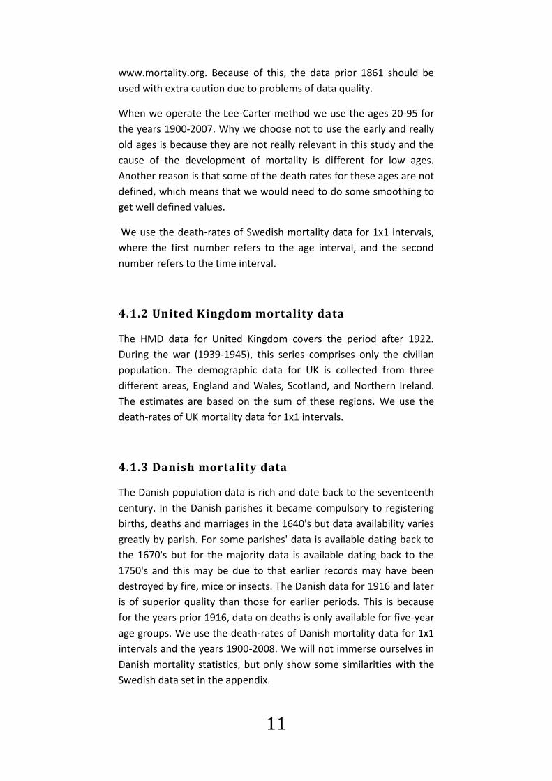
A pattern of mortality improvement means that we see

reduced mortality for certain age groups during certain

periods. In the following figures (figure 8-11) we can see the

deviations in the Lee-Carter model using data for Sweden

and United Kingdom. Different colors are used for different

percentages, the lower the percentage the fewer deaths,

i.e. mortality improvement. If we compare at the

corresponding figures for Sweden and United Kingdom we

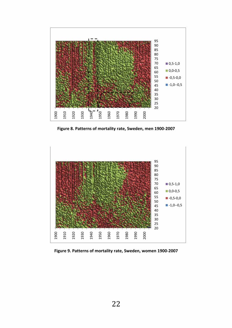
can see some big differences. In the UK figures (figures 10

and 11), there are clear signs of mortality improvements for

the cohort born around 1931. In the figures for Swedish

data we can see some kind of patterns but not as clear as

for United Kingdom.

The vertical line that appears just before 1945 in the

Swedish figures (figure 8 and 9), is an indirect effect of the

tuberculosis vaccine and the following mortality

improvement a consequence of it.

22

Figure 8. Patterns of mortality rate, Sweden, men 1900-2007

Figure 9. Patterns of mortality rate, Sweden, women 1900-2007

20253035404550556065707580859095

19

00

19

10

19

20

19

30

19

40

19

50

19

60

19

70

19

80

19

90

20

00

0,5-1,0

0,0-0,5

-0,5-0,0

-1,0--0,5

20253035404550556065707580859095

19

00

19

10

19

20

19

30

19

40

19

50

19

60

19

70

19

80

19

90

20

00

0,5-1,0

0,0-0,5

-0,5-0,0

-1,0--0,5

23

Figure 10. Patterns of mortality rate, UK, men 1922-2006

If we look at the ages 20-35 for the years around 1942 we can see

some differences in colors. These differences in mortality are

because of the high amount of young men who died during the war.

This rubs off on the generations that are not in war. Due to large

losses, it results in fewer babies in the next generation.

After contact with Mr. Adrian Gallop* we concluded that one possible

reason for the diagonal line that we can see in both male and female

figures for United Kingdom might be that the there was a rapid

change in the birth rate/number of births during the years 1919 and

1920 (and possibly 1918 also). Effectively it means that using the mid-

year population estimates as the exposed to risk for these cohorts is

not as reliable as for other birth years as the births for these cohorts

were not spread evenly over those years and hence may lead to a

significant under or over count for those years compared to

calculations on a daily basis, if we had that data available.

* A. Gallop, Government's Actuary Department, UK, personal contact

20

25

30

35

40

45

50

55

60

65

70

75

80

85

90

95

19

22

19

32

19

42

19

52

19

62

19

72

19

82

19

92

20

02

0,5-1,0

0,0-0,5

-0,5-0,0

24

If we look at figure 11 there are some patterns which indicate that

women in their 50's (year 2002) have had mortality improvement. It

is too early to say anything about this, but it could be a good idea to

follow up on this particular group. Similar patterns can be found for

the same age and gender in Denmark.

Figure 11. Patterns of mortality rate, UK, women, 1922-2006

The corresponding figures G and H for Danish data can be found in

appendix A. Those figures are quite interesting compared to Swedish

data. It is possible to see mortality improvement for both men and

women but at different time periods. For men, there is an

improvement for the generation born around 1940 and for the

women it started a little bit earlier. There also seem to be some kind

of pattern for women that were in there 50's in 2000.

20

25

30

35

40

45

50

55

60

65

70

75

80

85

90

95

19

22

19

32

19

42

19

52

19

62

19

72

19

82

19

92

20

02

0,4-0,6

0,2-0,4

0,0-0,2

-0,2-0,0

-0,4--0,2

-0,6--0,4

25

6. Fitting and applying the Renshaw-Haberman

model

6.1 Data

When we apply the Renshaw-Haberman model we use the same

datasets as earlier. We choose a specific time interval and a specific

age to see if there are any signs of cohort effects for those

generations.

We use the death-rates and exposure of risk of Swedish, English and

Danish mortality data for 1x1 intervals, where the first number refers

to the age interval, and the second number refers to the time

interval.

6.2 Parameter estimation for the Renshaw-

Haberman model

We let the random variable denote the number of deaths in a

population at age x and time t.

We can estimate the central mortality rate as

where represent the number of deaths and represent the

matching central exposure for any given subgroup. We let

define the combination of age and period, i.e. the cohort year. To get

the best estimates we approach a seven-step method, (Butt and

Haberman, 2009).

1. To estimate the parameters in the Renshaw-Haberman model

we use a pre-programmed software for R named LifeMetrics.

As in the Lee-Carter model we start to estimate the fixed age

effects, but here we use the singular value decomposition

(SVD) method to find the least squares solution.

26

2. After that we will try to get appropriate initial values

Estimate the simplified period-cohort predictor, with the

constraints that

to get initial values for and .

⟶ calculate the adapted values

⟶ calculate the deviance .

3. We continue by updating the parameter

where ω is either 0 for every empty data cells and 1 for every

non-empty data cell.

- shift the updated parameter such that ;


⟶ calculate deviance .

4. Update parameter



27

5. Update parameter

- shift the updated parameter such that ;



6. Update parameter



7. Control the divergent convergence

where D is the deviance from step 3 and is the updated

deviance at step 6.

if ⟹ go to step 3.

stop iterate process when and take the

adapted parameters as the ML estimates to the

observed data.

Alternatively, stop if for 5 updating cycles in a

row and consider using other starting values or declare

the iterations non-convergent.

8. When convergence is achieved, rescale the new interaction

parameters

:

28

in order to satisfy the age-period Lee-Carter model

constraints

29

6.3 Adapt the parameters in the Renshaw-

Haberman model using R

The main reason for all those calculations is of course to predict

future mortality, i.e. forecasting life. To get even better estimates

and to forecast mortality we continue by using the statistical program

R. It is not possible to get good parameter values for the Renshaw-

Haberman method in Excel since we have to iterate so many times.

Before we have a look at the parameters we make residual plots for

the Renshaw-Haberman method for the different ages and periods to

see if any patterns are revealed.

As before we begin by looking at data for Sweden for the ages 20-95

during the period 1900-2007. The deeper the colour, the stronger are

the rates of improvement, i.e. lower mortality. The corresponding

figures for Swedish and British men are to be found in figures I and J

in appendix A.

Figure 12. Women, Sweden, 1900-2007

1900 1920 1940 1960 1980 2000

20

30

40

50

60

70

80

90

Year

Ag

e

30

Having a closer look at figure 12 for ages 50-95, we can spot that

there is some sort of mortality improvement for Swedish women

around 50 years old, born 1900-1910. This can be compared to the

patterns that are to be found in the British and Danish data sets of

figures 14 and K.

Figure 13. Ages 50-90, Swedish women, 1850-2007

Figure 14. United Kingdom 1922-2006, women

1900 1950 2000

50

60

70

80

90

Year

Ag

e

1940 1960 1980 2000

20

30

40

50

60

70

80

90

Year

Ag

e

31

Figure 15 shows parameter values in the Renshaw-Haberman model

for Swedish women, the corresponding figures for men are to be

found in figure M of appendix A. As we can see there is an extra

parameter that depends on time of birth. In section 9 we will, with

help of these values, calculate the reserve for a hypothetical

individual insurance company.

Figure 15. Age-period regression for Sweden, women

The parameter values are 0 at the beginning and the end due to the

parameter restriction in the adjustment. It is to get an unambiguous

alignment.

65 70 75 80 85 90 95

-4.0

-3.5

-3.0

-2.5

-2.0

-1.5

-1.0

Age

ax

Main age effects

65 70 75 80 85 90 95

0.0

24

0.0

28

0.0

32

0.0

36

Age

bx 1

Period Interaction effects

65 70 75 80 85 90 95

0.0

24

0.0

28

0.0

32

0.0

36

Age

bx 0

Cohort Interaction effects

Calendar year

kt (p

ois

son)

1900 1920 1940 1960 1980 2000

-25

-20

-15

-10

-50

Period effects

Year of birth

itx (

pois

son)

1800 1820 1840 1860 1880 1900 1920 1940

-10

010

20

Cohort effects

Age-Period-Cohort LC Regression for sweden [female]

32

7. Reserving with Lee-Carter

In all kind of business, buyers and sellers have to meet the specific

requirements so that both parties will be satisfied. In insurance, this

means that if an individual is insured, he/she expects to get

compensated in case of loss, damage or injury. To be prepared for

forthcoming and unpredictable disbursements each company makes

technical provisions. In life insurance, incoming and outgoing cash

flows are taking place at different times and the outgoing payments

will take place over a long period of time in the future.

7.1 Data

For simplicity we calculate the reserves by looking at two groups of

1000 people at a time, men and women separately. The inception we

use here is 2007, because that is the latest year from which we have

information for the Swedish population. The populations we will use

is one group of people that retires in 2007 and another group that

will retire in 10 years ahead of 2007, i.e. in 2017. We use the general

retirement age in Sweden which is 65. Every year, each individual in

the group of 1000 is expecting an amount of money. Therefore, it is

important to know what age the people in the test groups will reach.

7.2 Forecasting

When the data is adapted to the model, in the first case, the Lee-

Carter model, we already have values of the vectors and

historic values of , so future mortality rates are derived by

projecting the mortality index . The easiest way do to this is to use

linear regression. Simple linear regression assumes that a straight line

can be fitted to the data and the regression is .

We look at three different time periods, 1900-2007, 1960-2007 and

1980-2007 to find out how the outcome differs depending on the

forecasts we get. The longer forecast we would like to do, the further

back in time should we go for retrieving data. We have made a

forecast of 40 years and predicted that mortality is about 40% for age

33

96-105 and 100% for age 106 and older, i.e. the entire test group has

passed away.

In figure 16, we used historical data of the time trend index of

generally mortality, . We perform linear regression and assume

that mortality will follow the same curve the following 40 years. By

using different time periods we get different predictions of future

mortality. In the first figure we get a clear view of the mortality

during the last century. The different colours show the different time

periods we chose for our upcoming calculations and the three-drawn

lines show the linear regression for each time period.

Figure 16. Historical values of , 1900-2007, women

In figures 17-19 we see the different regressions we get from each

time period. Note that there are different dates on the x-axes of the

figures.

When we look at the entire time interval, 1900-2007, we get a

negative slope that decreases with 0,1819 per year, see figure 17.

-15

-10

-5

0

5

10

15

19

00

19

10

19

20

19

30

19

40

19

50

19

60

19

70

19

80

19

90

20

00

34


By using the time period 1960-2007 we get a negative slope of

0,1266 per year, see figure 18 and by using the time period 1980-

2007 we get a negative of 0,1464 per year, see figure 19.


Figure 19. Historical values of , 1980-2007

-15

-10

-5

0

5

10

15

18

90

19

00

19

10

19

20

19

30

19

40

19

50

19

60

19

70

19

80

19

90

20

00

20

10

20

20

-10

-8

-6

-4

-2

0

19

50

19

60

19

70

19

80

19

90

20

00

20

10

-10

-8

-6

-4

-2

0

1975 1980 1985 1990 1995 2000 2005 2010

35

7.3 Prospective reserving

The reserve for life insurance can be calculated either prospectively

or retrospectively. We will get the same results if the assumptions

are the same when calculating the reserve and calculating the

premium. The prospectively estimated reserve corresponds to the

present value of expected future pension benefits minus the present

value of expected future premiums which are being paid during the

contract period.

If we use the Lee-Carter model to predict the mortality index factor,

we have a reasonable image of what the mortality will be in the

future. We get

(9)

where denotes the fraction of the cohort alive at age and

is obtained by taking the exponential function of (1).

Figure 20. One-year death probabilities, , by calendar year 1900-

2007, men and women, permille

It is well known that women normally have a lower mortality rate

than men. In the figure above we see how the yearly expected

0,00

0,05

0,10

0,15

0,20

0,25

0,30

0,35

0,40

0,45

65 70 75 80 85 90 95

Men

Women

36

mortality looks for men and women when calculated on 1900-2007.

As mentioned in section 2 the life expectancy at birth for women is

around 83 years and around 79 years for men. When talking about

one-year death probabilities we mean how the death probability

changes for a given individual when he/she is getting older.

8. Reserve calculations for Lee-Carter

8.1 Zero interest rate with generation retiring

2007

Immediate annuity

One simple way to calculate the reserve is to calculate with zero

interest rate, i.e. the annuities are fixed and we assume that there is

no return on our funds (except maybe for expenses). This means that

we will put away exactly the amount of money that will be needed in

payments. Or we could use a fixed interest, which is the same thing

as having the same interest rate over the whole period.

where, is the interest capital and is the rate of interest and is

the capital that we need to put aside. In our case we will assume that

the constant interest is 2 percent per year.

In order to estimate the life expectancy when not using any interest

at all, we just have to calculate how many payments we will have to

make for the chosen group of people. We do this by summing years

of life beyond 65 in the test group and then divide the number of

people in the test group. This will give us the average life expectancy

at age 65.

For the three time-periods we have get different life expectancies

and this will make a difference in future payments.

37

To derive the life expectancy we have used (Andersson, 2005) and

we refer to this book for more details.

Let be a non-negative random variable that represents the

remaining life expectancy for an individual aged 65. The distribution

function is then defined as

The function is then defined as the survivor function

Simplification gives us

which can be written as

The life expectancy at age 65 is

38

We get the following results. Please note to that this is life

expectancy given an attained age, in this case an age of 65 and hence

is not the same life expectancies treated in section 2.

1900-2007 1960-2007 1980-2007

Men 16,48 16,39 16,61

Women 20,27 20,03 20,12

Table 3. Life expectancies at age 65 for men and women based of

different periods of estimation

If we look at the results for the three different predictions, the

differences may be relatively small, but in a large insurance company

the group of annuitants is very large and for each person one year

corresponds to quite a large amount of money.

8.2 Compound interest with generation retiring

2007

The compound interest

(10)

The capital grows exponentially and we can use the term

for the interest intensity.

In order to find out the amount of money we need to put away for

upcoming payments with 2 percent interest we need to use a

discount factor. The discount factor we get by discounting according

to

39

we get the interest intensity. The discount factor id defined as

We assume that all payments from policyholders are made in January

2007 and all the disbursements are made in December. That provides

the reserve an additional year with interest. If we look at the results

in table 4, we see the total amount of money that is to be needed to

fulfill the commitments to the policyholders. If we then look at the

results in table 5, we see how large the technical provision needs to

be. If we subtract the results in table 4 with the results in table 5 we

see how much the company would save on reserving with 2 percent

interest.

We get the following results

Historic period used

Reserve

1900-2007

1960-2007

1980-2007

Men 16 482,78 16 417,72 16 609,78 Women 20 273,99 20 028,67 20 116,36

Table 4. Reserving with zero interest per 1000 policyholders, whole

life annuity


Reserve

1900-2007

1960-2007

1980-2007

Men 13 479,59 13 437,02 13 562,53 Women 16 090,25 15 935,30 15 990,74

Table 5. Reserving with 2% interest per 1000 policyholders, whole

life annuity

40

If we assume that we looking at the whole period, i.e. 1900-2007 and

then calculate the differences between that period and the other two

periods, and continue with comparing 1960-2007 with 1980-2007 we

get the following table (table %). In table 6 we compute the reserve

at 2007 with 2 percent interest rate based on estimates for a historic

period 1900-2007 and then calculate the difference between this

reserve and those based on the same interest rates but period 1960-

2007 and 1980-2007. As we can see, the time period differences are

within 1 percent but if we compare the two tables (table 4 and 5)

we get that the effect of discounting is much larger. There is a

decrease of about 20 percent whichever period or gender that is

chosen.

1900-2007 1960-2007 1980-2007

Men 13 479,59 -42,57 (-0,316%)

+82,94 (+0,615%)

Women 16 090,25 -154,95 (-0,963%)

-99,51 (-0,618%)

Men 13 437,02 +125,51 (+0,934%)

Women 15 935,30 +55,44 (+0,348%)

Table 6. Differences between the three periods

8.3 Generation retiring 2017 with zero- and

compound interest

We use the same calculations as before, except for another group of

people. This time the people are 55 years old at 2007. A single

premium is paid in January and the annuity payments will start at

2017.


Reserve

1900-2007

1960-2007

1980-2007

Men 15 284,16 15 159,19 15 528,19 Women 19 878,36 19 440,76 19 597,49

Table 7. Reserving with zero interest per 1000 policyholders, life

annuity deferred by 10 years

41


Reserve

1900-2007

1960-2007

1980-2007

Men 10 221,97 10 151,77 10 358,46 Women 12 878,89 12 644,94 12 728,87

Table 8. Reserving with 2% interest per 1000 policyholders, life


In table 9 we can see the differences between the three time periods.

Depending on what historic period we use we get different possible

reserves. There are effects in the time periods, depending on which

two periods we choose between, mostly of them in the interval 1,5

percent, which can make a big difference in payments for the

insurance company if they have many policyholders and many

commitments.

To see how much the company would save on reserving with 2

percent interest compared to zero interest, we subtract those of

table 7 with the results in table 8. We note again that the effects

caused by the periods are small compared with the effects from

discounting, where there are reductions higher than 33 percent

whichever time period we choose.

1900-2007 1960-2007 1980-2007

Men 10 221,92 -70,15 (-0,686%)

+136,54 (+1,336%)

Women 12 878,89 -233,95 (-1,817%)

-150,02 (-1,165%)

Men 10 151,77 +206,69 (+2,036%)

Women 12 644,94 +83,93 (0,664%)

Table 9. Differences between the three periods, deferred life

annuity

To find out what difference it makes if the policyholders make their

payment when they are 55 compared to when they are 65 we

compare table 5 and table 8. As we can see it takes less money in the

42

technical provision, the earlier the policies are made. If we assume

that the premiums are the same for the policyholders, then the

insurance company can save between 19,96 and 24,37 percent on

the extra ten years depending on what time period and gender they

based their calculations on.

8.4 Variable interest

In reality, nowadays it is getting more common to use variable interest, which makes it more difficult to predict how large the technical provisions need to be. The individual insurer cannot itself affect the interest since it is controlled by the banks and the government.

(11)

For practical reasons we will not make any calculations with variable

interest.

43

9. Reserving with Renshaw-Haberman

9.1 Forecasting

When calculate the reserve with the Renshaw-Haberman method we

assume the same conditions as in section 7.2. In figures 21 and 22,

we used historical data of the time trend index of generally mortality,

. We perform linear regression and assume that mortality will

follow the same curve the following 40 years. By using different time

periods we get different predictions of future mortality. The different

colours show the different time periods we chose for our upcoming

calculations and the three-drawn lines show the linear regression for

each time period. As we can see they differ from the k-values in the

Lee-Carter model.

Figure 21. Historical values of , 1900-2007, men

-18,00

-16,00

-14,00

-12,00

-10,00

-8,00

-6,00

-4,00

-2,00

0,00

19

00

19

10

19

20

19

30

19

40

19

50

19

60

19

70

19

80

19

90

20

00

44


In figure 22 it is easy to see how wrong the predictions might be if we

only look at a short time of historical mortality. The curve is

decreasing all the way from year 1900 to the 1980 and then it starts

increasing. In section 10 we will see how this affects the reserving. In

the following three figures we see the different regressions we get

from each time period. Note that there are different years on the x-

axes.

When we look at the entire time interval, 1900-2007, we get a

negative slope of 0,2781 per year, as seen in figure 23.


By using the time period 1960-2007 we get a positive slope of 0,0518

per year, as shown in figure 24 and by using the time period 1900-

-70,00

-60,00

-50,00

-40,00

-30,00

-20,00

-10,00

0,00

19

00

19

10

19

20

19

30

19

40

19

50

19

60

19

70

19

80

19

90

20

00

-50,00

-40,00

-30,00

-20,00

-10,00

0,00

18

90

19

00

19

10

19

20

19

30

19

40

19

50

19

60

19

70

19

80

19

90

20

00

20

10

20

20

45

2007 we get a positive slope that increase with 0,2905 per year, as

shown in figure 25.



10. Reserve calculations for Renshaw-Haberman

10.1 Generation retiring 2007

To calculate the reserve using the Renshaw-Haberman method we

use the same derivation as in section 8.1 and 8.2.

We assume that all payments from policyholders are made in January

2007 and all the disbursements are made in December. That provides

the reserve an additional year with interest. If we look at the results

in table 10, we see the total amount of money that is to be needed to

fulfill the commitments to the policyholders. And if we look at the

results in table 11, we see how large the technical provision needs to

be. If we subtract the results in table 10 with those of table 11 we see

-40,00

-30,00

-20,00

-10,00

0,00

19

50

19

60

19

70

19

80

19

90

20

00

20

10

-40,00

-30,00

-20,00

-10,00

0,00

19

70

19

80

19

90

20

00

20

10

46

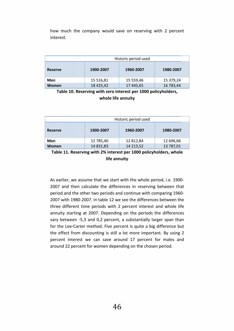
how much the company would save on reserving with 2 percent

interest.


Reserve

1900-2007

1960-2007

1980-2007

Men 15 516,81 15 559,46 15 379,24 Women 18 425,42 17 445,65 16 783,44

Table 10. Reserving with zero interest per 1000 policyholders,

whole life annuity


Reserve

1900-2007

1960-2007

1980-2007

Men 12 785,40 12 812,84 12 696,66 Women 14 831,83 14 213,52 13 787,01

Table 11. Reserving with 2% interest per 1000 policyholders, whole

life annuity

As earlier, we assume that we start with the whole period, i.e. 1900-

2007 and then calculate the differences in reserving between that

period and the other two periods and continue with comparing 1960-

2007 with 1980-2007. In table 12 we see the differences between the

three different time periods with 2 percent interest and whole life

annuity starting at 2007. Depending on the periods the differences

vary between -5,3 and 0,2 percent, a substantially larger span than

for the Lee-Carter method. Five percent is quite a big difference but

the effect from discounting is still a lot more important. By using 2

percent interest we can save around 17 percent for males and

around 22 percent for women depending on the chosen period.

47

1900-2007 1960-2007 1980-2007

Men 12 785,40 +27,44 (+0,215%)

-88,74 (-0,694%)

Women 14 831,83 -618,31 (-4,169%)

-1044,82 (-7,044%)

Men 12 812,84 -116,18 (-0,907%)

Women 17 235,04 -426,51 (-3,001%)

Table 12. Differences between the three periods

10.2 Generation retiring 2017

A group of 55 year olds are buying a single premium in January 2007.

That gives us a period of ten years before the first payment is made.

We get the following results:


Reserve

1900-2007

1960-2007

1980-2007

Men 17 389,37 17 842,32 18 395,16 Women 19 535,34 18 639,37 18 002,04

Table 13. Reserving with zero interest per 1000 policyholders, life



Reserve

1900-2007

1960-2007

1980-2007

Men 11 402,29 11 645,34 11 940,19 Women 12 643,97 12 173,63 11 835,60

Table 14. Reserving with 2% interest per 1000 policyholders, life


In order to find out what difference it makes if the policyholders

make their payment when they are 55 and 65 we compare table 10

with table 13 and then table 11 with table 14. When looking at whole

life annuity with zero interest the technical provision is larger for the

55 year olds. At first thought, one would think that it would be

48

cheaper for that group since some individuals will die before

payments begin. Especially for then men hence they have greater

mortality in this age then women. But this generation will also live

longer and that effect is stronger, which means that the technical

provision increases. In the other comparison we get the same

conclusion as before; it takes less money in technical provision the

earlier the policies are made. If we make the same assumptions as

before, i.e. that the price the insured is paying is independent of the

start of payment, then the insurance company can then save 5,96 to

10,82 percent for men and 28,91 to 29,70 percent for women

depending on the time period used for parameter estimation.

1900-2007 1960-2007 1980-2007

Men 11 402,29 +243,05 (+2,132%)

+537,90 (+4,717%)

Women 12 643,97 -470,34 (-3,720%)

-808,37 (-6,393%)

Men 11 645,34 +294,85 (+2,532%)

Women 12 173,63 -338,03 (-2,777%)

Table 15. Differences between the three periods, deferred life

annuity

In table 15 we see the differences between the three time periods,

calculating with 2 percent interest. Depending on what historic

period we use we obtain different reserves. The effects of time

period are larger for the Renshaw-Haberman method than for the

Lee-Carter method. With deferred whole life annuity the effects are

between -6,4 and +4,7 percent. If we subtract the results in table 13

with those of table 14 we see how much the company would save on

reserving with 2 percent interest compared to zero interest. We

notice once again that the effects caused by time period are much

smaller than those caused by discounting, where there is reduction is

around 35 percent whichever timer period or gender we choose.

Compared to reserving with the Lee-Carter model we get much

bigger differences when reserving with the Renshaw-Haberman

49

model. Especially for women since their mortality time trend index

curve looks very different depending on what time period we focus

on. The time index curve decreases until around 1980 but then starts

increasing. There are differences in technical provisions up to 6

percent and that may cause huge miscalculations. Consequently, the

differences in reserving can be very large depending on the historical

data we choose to use.

11. Comparison of results between the different

methods

Women 1900-2007 1960-2007 1980-2007

Lee-Carter -0,963% -0,618% Renshaw-Haberman

-3,092% -5,335%

Lee-Carter 0,348% Renhaw-Haberman

-2,314%

Table 16. Differences for generation retiring 2007 per 1000

policyholders, women

Women 1900-2007 1960-2007 1980-2007

Lee-Carter -1,817% -1,165% Renshaw-Haberman

-3,720%

-6,393%


-2,777%

Table 17. Differences for generation retiring 2017 per 1000

policyholders, women

Comparing the results of technical provisions using the different

models (table 16 and 17) we can see that the differences between

periods are much larger for the Renshaw-Haberman model than for

the Lee-Carter model. This is true for the immediate as well as for the

deferred annuity. On the other hand, the Renshaw-Haberman and

Lee-Carter models yield similar differences in reserving between zero

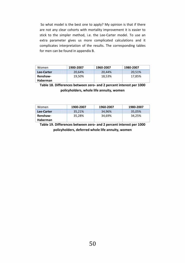
and two percent interest rate, as shown in tables 18 and 19.

50

So what model is the best one to apply? My opinion is that if there

are not any clear cohorts with mortality improvement it is easier to

stick to the simpler method, i.e. the Lee-Carter model. To use an

extra parameter gives us more complicated calculations and it

complicates interpretation of the results. The corresponding tables

for men can be found in appendix B.

Women 1900-2007 1960-2007 1980-2007

Lee-Carter 20,64% 20,44% 20,51% Renshaw-Haberman

19,50% 18,53% 17,85%

Table 18. Differences between zero- and 2 percent interest per 1000

policyholders, whole life annuity, women

Women 1900-2007 1960-2007 1980-2007


35,28% 34,69% 34,25%

Table 19. Differences between zero- and 2 percent interest per 1000

policyholders, deferred whole life annuity, women

51

12. Conclusions

Differences in mortality have always existed and always will. The

complicated thing is to predict it.

What are the consequences of a reduced mortality? That depends on

when the reduction starts showing. If it is only one generation that

makes extra mortality improvement, there is a risk that these

individuals have to fight more for their survival. Compare for example

a baby boom, i.e. a time period during which many more babies are

born. Everyone needs kindergarten places, primary education and

jobs in the future. But the advantage of continuing mortality

improvement from birth is that the society in the meantime has more

time to acclimatize. It makes it more complicated if the

improvements are shown later, for example when the members of

the generation are around 40 years old and continue having

improvements for the rest of their lives.

In this survey, we have seen many patterns of mortality

improvement. But when looking at mortality improvement it is

difficult to decide whether it is just normal improvement or if it is

large enough to be called a cohort effect. The reason that mortality

improvement has been so great the last thousand years depends

largely on medical progress and improved standard of living. The

general improvement should soon come to a standstill. So in the

future, it may be easier to distinguish cohort effects from usual

mortality improvement.

My conclusion is that it is possible to find more evidence of birth

cohort effects if we have lower requirements about what an effect is.

It is in the researcher's requirements and accuracy. "There is nothing

like looking, if you want to find something. You certainly usually find

something, if you look, but it is not always quite the something you

were after" (J.R.R Tolkien). In many ways, there are good patterns,

but I do not think that there are any patterns of mortality

improvement that last long enough time to be called a birth cohort

effect.

Either way, it is really important for insurers to have a reasonable

good overview of what future mortality will look like. The most

difficult about this is to make a decision about how many years of

52

historical data one should use to get the most successful prediction.

A good rule of thumb is that the longer forecast we would like to do,

the further back in time should we go for data retrieval. But this

depends of course on what the historical data look like. If there are

many specific events in history that make mortality change much

over short periods, it is a good idea to make some form of smoothing

to get a better result.

What effects will a mortality improvement have on the insurers? A

predicted improvement should not have any effect on the individual

company, since they have had the option to prepare themselves. The

technical provisions would be made larger in order to cover future

payments. But if not, it could mean a major loss of money, with

further payments. A difference in a few percent in our computations

of future payments can make a huge difference for the insurer.

The patterns of mortality improvement that were seen for women in

United Kingdom and Denmark could be interesting to follow up in a

few years to find out if they are still making progress. However, it

may be too late to make any changes for insurers since this

generation has already passed the age of 60 and begun to retire.

To calculate the technical provision we have used two different

models, the Lee-Carter model and the Renshaw-Haberman model.

Since we only applied the models for reserving on Swedish data, we

can't draw any firm conclusions. The Renshaw-Haberman model is an

extended version of Lee-Carter with an extra parameter. It can give

inconclusive results if we make the wrong forecasts. But possibly the

big differences in our results between the Renshaw-Haberman and

Lee-Carter models may be due to the Swedish time trend index .

An important result is that regardless of which model we decided to

use, and in all different scenarios that we set up; the effect of

discounting was a lot larger than the time period effect. The effect of

discounting was also very similar for the two models, while the effect

of chosen historical time period differed more. That gives us the

implication, that as sooner the insurers begin with reserving, the

better.

53

13. Appendix A.

Figure A. General pattern of mortality , Sweden, 1751-2007, men

and women

Figure B. The mortality trend , Sweden, 1751-2007, men and

women

-8,00000

-7,00000

-6,00000

-5,00000

-4,00000

-3,00000

-2,00000

-1,00000

0,00000

20 30 40 50 60 70 80 90

Men

Women

-20

-15

-10

-5

0

5

10

15

1751 1801 1851 1901 1951 2001

Men

Women

54

Figure C. Age-specific constant , Sweden, 1751-2007, men and

women

Figure D. General pattern of mortality , United Kingdom, 1922-

2006, men and women

0

0,02

0,04

0,06

0,08

0,1

0,12

0,14

0,16

0,18

0,2

20 30 40 50 60 70 80 90

Men

Women

-8

-7

-6

-5

-4

-3

-2

-1

0

20 30 40 50 60 70 80 90

Men

Women

55

Figure E. The mortality trend , United Kingdom, 1922-2006, men

and women

Figure F. age-specific constant , United Kingdom, 1922-2006, men

and women

-8

-6

-4

-2

0

2

4

6

8

10

19

22

19

32

19

42

19

52

19

62

19

72

19

82

19

92

20

02

Men

Women

0

0,05

0,1

0,15

0,2

0,25

20 30 40 50 60 70 80 90

Men

Women

56

Figure G. Mortality pattern, Denmark, women, 1900-2008

Figure H. Mortality pattern, Denmark, men, 1900-2008

20253035404550556065707580859095

19

00

19

10

19

20

19

30

19

40

19

50

19

60

19

70

19

80

19

90

20

00

0,50-1,00

0,00-0,50

-0,50-0,00

-1,00--0,50

-1,50--1,00

20253035404550556065707580859095

19

00

19

10

19

20

19

30

19

40

19

50

19

60

19

70

19

80

19

90

20

00

0,5-1,0

0,0-0,5

-0,5-0,0

-1,0--0,5

57

Figure I. Men Sweden, 1900-2007

Figure J. Men, UK, 1922-2007

1940 1960 1980 2000

20

30

40

50

60

70

80

90

Year

Ag

e

1900 1920 1940 1960 1980 2000

20

30

40

50

60

70

80

90

Year

Ag

e

58

Figure K. Age-period regression for Sweden, male

Figure L. Historical values of , 1900-2007, men

-8,00

-6,00

-4,00

-2,00

0,00

2,00

4,00

6,00

8,00

10,00

12,00

19

00

19

10

19

20

19

30

19

40

19

50

19

60

19

70

19

80

19

90

20

00

65 70 75 80 85 90 95

-3.5

-3.0

-2.5

-2.0

-1.5

-1.0

Age

ax

Main age effects

65 70 75 80 85 90 95

0.0

20

0.0

25

0.0

30

0.0

35

0.0

40

Age

bx 1

Period Interaction effects

65 70 75 80 85 90 95

0.0

20

0.0

25

0.0

30

0.0

35

Age

bx 0

Cohort Interaction effects

Calendar year

kt (p

ois

son)

1900 1920 1940 1960 1980 2000

-15

-10

-50

Period effects

Year of birth

itx (

pois

son)

1800 1820 1840 1860 1880 1900 1920 1940

-15

-10

-50

510

Cohort effects

Age-Period-Cohort LC Regression for sweden [male]

59

Figure M. Historical values of , 1900-2007, decrease with 0,1259

per year

Figure N. Historical values of , 1960-2007, decrease with 1,1032

per year

Figure O. Historical values of , 1980-2007, decrease with 0,9777

per year

-10,00

-5,00

0,00

5,00

10,00

15,00

1880 1900 1920 1940 1960 1980 2000 2020

-8,00

-6,00

-4,00

-2,00

0,00

1950 1960 1970 1980 1990 2000 2010

-8,00

-6,00

-4,00

-2,00

0,00

1975 1980 1985 1990 1995 2000 2005 2010

60

14. Appendix B.

Men 1900-2007 1960-2007 1980-2007

Lee-Carter -0,423% 0,615% Renshaw-Haberman

0,215%

-0,694%


-0,907%

Table AA. Differences for generation retiring 2007, men

Men 1900-2007 1960-2007 1980-2007

Lee-Carter -0,686% 1,336% Renshaw-Haberman

2,132%

4,717%


2,532%

Table BB. Differences for generation retiring 2017, men

Men 1900-2007 1960-2007 1980-2007


17,60% 17,65%

17,44%

Table CC. Differences between zero- and 2 percent interest, whole

life annuity, men

Men 1900-2007 1960-2007 1980-2007


34,43%

34,73%

35,09%

Table DD. Differences between zero- and 2 percent interest,

deferred whole life annuity, men

61

15. References Books and Journals

Adam, L. (2003). Canadian pensioner's mortality 1967-2000;

Vancouver: School of actuarial science

Alm, E., Andersson, G. von Bahr, B., Martin-Löf, A. (2006).

Livförsäkringsmatematik 2; Stockholm: Elanders Gotab AB

Anderssonm, G. (2005). Livförsäkringsmatematik; Stockholm:

Elanders Gotab AB

Andreev, K., and Vaupel, J. (2005). Patterns of mortality improvement

over age and time in developed countries: estimation, presentation

and implications for mortality forecasting

Bahr, B (2006). Skatta parametrarna i Lee-Carters modell för

dödlighet; Working paper, DUS

Booth, H., Maindonald, J. and Smith, L. (2002). Age-time interactions

in mortality projection: applying the Lee-Carter to Australia; The

Australian national University

Butt, Z. and Haberman, S. (2009). A collection of R functions for

fitting a class of Lee-Carter mortality models using iterative fitting

algorithms, London: Cass Business School, City University

Cairns, A., Blake, D. and Dowd, K. (2008). "Modelling and

management of mortality risk: a review," Scandinavian actuarial

journal 2008, 2-3, 79-113

Denuit, M. (2004). Lee-Carter model with Poisson random structure

and applications in insurance; Louvain-la-Neuve, Beligium: Université

catholique de Lovain. Workshop at Heriot-Watt University,

Edingburgh

Försäkringstekniska forskningsnämnden, Sveriges försäkringsförbund

(2007). Försäkrade i Sverige - dödlighet och livslängder, prognoser

2007-2050, Stockholm: Elanders Gotab AB

Gallop, A. (2008). Mortality projections in the United Kingdom;

Girosi, F. and King, K. (2007); Understanding the Lee-Carter mortality

forecasting method

62

Jacobsen, R., Keiding, N. and Lynge, E. (2001). Long term mortality

trends behind low life expectancy of Danish women; Copenhagen:

Institute of public health, University of Copenhagen.

Kirill, A. and James, V. (2006). Forecasts of cohort mortality after age

50; Rostock: Max-Planck-Institut für demografische Forschung

Lee, R. (1999) "Thee Lee-Carter method for forecasting mortality,

with various extensions and applications," North American actuarial

journal: Vol. 4, No. 1

Lee, R. and Carter, L. (2002). "Modeling and forecasting U.S

mortality," Journal of the American statistical association Vol. 87, No.

419

Li, S-H. and Chan, W-S. (?) The Lee-Carter model for forecasting

mortality revisited

Lundström, H. and Qvist, J. (2004). "Mortality forecasting and trend

shifts: an application of the Lee-Carter model to Swedish mortality

data," International Statistical Review: 72, 1, 37-50

Maxwell, A. The future of the social security pension provision of

Trinidad and Tobago using Lee-carter forecasts; London: Graduate of

Cass Business School, City University

Olsén, J. (2005). Modeller och projektioner för dödlighetsintensitet-

en anpassning till svensk populationsdata 1970-2004; Stockholm

Pitacco, E., Denuit, M., Haberman, S. and Olivieri, A. (2009).

Modelling longevity dynamics for pensions and annuity business; New

York: Oxford University Press Inc.

Renshaw, A. and Haberman, S. (2008). Extensions to the Lee-Carter

model, including risk measurement in the age-period-cohort versions

of the model; London: Cass Business School, City University

Renshaw, A. and Haberman, S. (2002). Lee-Carter mortality

forecasting: a parallel generalized linear modelling approach for

England and Wales mortality projections; London: City University

Renshaw, A. and Haberman, S. (2005). "Mortality reduction factors

incorporating cohort effects," Actuarial Research paper No. 160

63

Scherp, H. (2007). Applying the Lee-Carter model to countries in

Eastern Europe and the former Soviet Union; Stockholm: Master's

thesis

Sunamoto, N. (2005). Cohort effect structure in the Lee-Carter

residual term; Tokyo: Fukoku mutual life insurance company

Kingdom, J. (2008). "Mortality improvement" The Actuary (the

magazine for the actuarial profession), 01 May, 2008

Willets, R. (2004). The cohort effect: Insights and explanations;

Presented to the Faculty of actuaries March 2004, and to the

Institute of actuaries April 2004

Willets, R., Gallop, A., Leandro, P., Lu, J., MacDonald, A., Miller, K.,

Richards, S., RobJohns, N., Ryan, J. and Water, H. (2004). Longevity in

the 21st century; Presented to the Faculty of actuaries March 2004,

and to the Institute of actuaries April 2004

Wohlfart (2006). Evaluation of the LC method based on Sweden and

Denmark demographics; Stockholm: Master's thesis, Stockholm

University

Zheng Wang, J. (2007). Fitting and forecasting mortality for Sweden:

Applying the Lee-Carter model; Stockholm: Master's thesis

Internet references

Information about tuberculosis in Sweden is available at

http://www.epiwebb.se/22_TB/historik.shtml

JPMorgan Pension Advisory Group (Nov 2007). LifeMetrics, The

software can be downloaded from the LifeMetrics website:

www.jpmorgan.com/lifemetrics

cohort eﬀects in swedish mortality and their eﬀects … · longevity risk martina gustafsson...

Documents