cointegration tests in the presence of structural breaks

EISEVIER

JOURNAL OF Econometrics

Journal of Econometrics 70 (1996) 187-220

Cointegration tests in the presence of structural breaks

Julia Campos”, Neil R. Erics.son*‘b, David F. Hendry”

‘Departamento de Economia e Historia Econbmica, Universidad de Salamanca, 37008 Salamanca, Spain

blnternational Finance Division, Federal Reserve Board, Washington, DC 20551, USA ‘Nufield College, Oxford OXI INF, UK

Abstract

Structural breaks in stationary time series can induce apparent unit roots in those series. Thus, using recently developed recursive Monte Carlo techniques, this paper investigates the properties of several cointegration tests when the marginal process of one of the variables in the cointegrating relationship is stationary with a structural break. The break has little effect on the tests’ size. However, tests based on estimated error correction models generally are more powerful than Engle and Granger’s two-step procedure employing the Dickey-Fuller unit root test. Discrepancies in power arise when the data generation process does not have a common factor.

Key words: Cointegration; Error correction; Monte Carlo; Structural breaks; Tests JEL classijcation: C12; Cl5

1. Introduction

Structural breaks in stationary time series can induce apparent unit roots, as

shown by Perron (1989) analytically and empirically and by Hendry and Neale (1991) via Monte Carlo. Consequently, tests of unit roots have low power when

*Corresponding author

The views expressed in this paper are solely the responsibility of the authors and should not be

interpreted as reflecting those of the Board of Governors of the Federal Reserve System or other

members of its staff. We are grateful to Peter Boswijk, Jean-Marie Dufour, Andreas Fischer, Eric

Ghysels, Peter Phillips, Carmela Quintos, and two referees for helpful comments, and to the U.K.

Economic and Social Research Council for financial support to the third author under grant

BOO220012. All numerical results were obtained using PCNAIVE Version 6.01 and PcGive Version

7.00; cf. Hendry and Neale (1990) and Doornik and Hendry (1992).

0304-4076/96/$15.00 0 1996 Elsevier Science S.A. All rights reserved

SSDI 030440769401689 W

188 J. Campos et al./Joumal of Economeirics 70 (1996) 187-220

applied to series with structural breaks. Conversely, such series mimic series with actual unit roots. Using Monte Carlo, this paper investigates the power of several cointegration tests when the marginal process of one of the variables in the cointegrating relationship contains a structural break. The detectability of the structural break itself is also examined, both by classical constancy tests and by recently introduced tests for invariance. The data include stationary and nonstationary series with breaks. Calculation and analysis of results employ recently developed Monte Carlo techniques, as described in Hendry (1984) and Hendry and Neale (1987, 1990).

A structural break has little effect on the size of the cointegration tests studied. However, the break does affect the power of cointegration tests when the process generating the data does not have a common factor. Specifically, tests based on estimated error correction models generally are more powerful than Engle and Granger’s (1987) commonly used ‘two-step’ procedure employing the Dickey- Fuller unit root test. The error-correction-based test uses available information more efficiently than the Dickey-Fuller test, paralleling Kremers, Ericsson, and Dolado’s (1992) results without a structural break.

Section 2 describes the data generation process for the Monte Carlo study, the test statistics considered, and some of their analytical properties. Section 3 presents the experimental design and simulation techniques. Section 4 examines the detectability of stationarity and of the break in the marginal process. Section 5 interprets the Monte Carlo results on the cointegration tests. Section 6 con- cludes. The Appendix derives asymptotic properties of the unit root estimator when the underlying process has a break.

2. The data generation process, the test statistics, and some analytical properties

This section describes the data generation process for the Monte Carlo simulation (Section 2.1), the test statistics studied (Section 2.2), and some analytical properties of those statistics (Section 2.3). The data generation process (DGP) is a first-order bivariate vector autoregressive process with a possible structural break in one of the variables’ processes. The test statistics are Dickey- Fuller (static regression) and error correction t-ratios, and each is considered with and without knowledge of the cointegrating vector (if it exists). Together, the DGP and the test statistics delimit the scope of the analysis. Some analytical properties of the test statistics prove helpful in interpreting the Monte Carlo evidence.

2.1. The data generation process

The DGP is a linear first-order vector autoregression with normal disturbances, Granger causality in only one direction, and a possible structural break

J. Campos et al. ,lJournal of Econometrics 70 (1996) 187-220 189

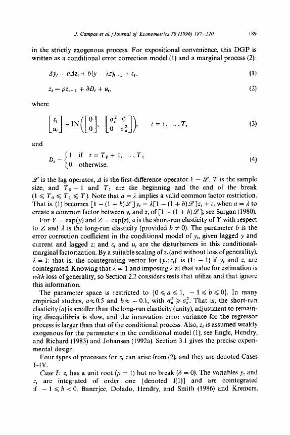
in the strictly exogenous process. For expositional convenience, this DGP is written as a conditional error correction model (1) and a marginal process (2):

dy, = aAzg + b(y - AZ),_ 1 + E,,

z,=pz,-g +m,+u,,

where

and

1 if t=T,-tl,...,T,

0 otherwise.

(1)

(2)

(4)

L? is the lag operator, d is the first-difference operator 1 - %“, T is the sample size, and T, + 1 and Ti are the beginning and the end of the break (1 d T,, d T1 < T). Note that a = 2 implies a valid common factor restriction. That is, (1) becomes [ 1 - (1 + b)5?]yl = A[1 - (1 + b)T]z, + E, when a = A to create a common factor between yt and z, of [l - (1 + b&L?]; see Sargan (1980).

For Y = expfy) and Z = exp(z), a is the short-run elasticity of Y with respect to Z and it is the long-run elasticity (provided b # 0). The parameter b is the error correction coefficient in the conditional model of y,, given lagged y and current and lagged z; and st and ut are the disturbances in this conditional- marginal factorization. By a suitable scaling of z, (and without loss of generality), 2 = 1: that is, the cointegrating vector for (yt:zt)’ is (1: - 1) if y, and z, are ~ointegrated. Knowing that I = 1 and imposing i at that value for estimation is with loss of generality, so Section 2.2 considers tests that utilize and that ignore this information.

The parameter space is restricted to {O 6 a < 1, - 1 4 b < O}. In many empirical studies, a ~0.5 and b x - 0.1, with 0,’ > 0,‘. That is, the short-run elasticity (a) is smaller than the long-run elasticity (unity), adjustment to remain- ing disequilibria is slow, and the innovation error variance for the regressor process is larger than that of the conditional process. Also, z, is assumed weakly exogenous for the parameters in the conditional model (1); see Engle, Hendry, and Richard (1983) and Johansen (1992a). Section 3.1 gives the precise experimental design.

Four types of processes for z, can arise from (2), and they are denoted Cases I-IV.

Case I: z, has a unit root (p = 1) but no break (6 = 0). The variables y, and z, are integrated of order one [denoted I(l)] and are cointegrated if - 1 d b < 0. Banerjee, Dolado, Hendry, and Smith (1986) and Kremers,

190 .I Campos et al/Journal of Econometrics 70 (1996) 187-220

Ericsson, and Dolado (1992) inter alia analyze the properties of various cointegration estimators and test statistics under this DGP, both analytically and by Monte Carlo.

Case II: z, is stationary (I pi < 1) with no break (6 = 0). Then, y, is I(1) if b = 0, and y, and z, are jointly stationary with an error correction representation if - 1 Q b < 0. Davidson, Hendry, Srba, and Yeo (1978) and Davidson and Hendry (1981) provide some asymptotic and Monte Carlo evidence on the properties of the error correction test statistic.

Case III: zt is I( 1) (p = 1) and has a break (6 # 0). If the break is large enough, z, may appear to be an I(2) process. Likewise, a trend-stationary variable with a break in the slope may appear I(2): the difference of the series has a break in mean. While Case III is of potential empirical interest, this paper only briefly considers it, in Section 4. However, see Johansen (1992b, 1992~) for theoretical and empirical analyses of I(2) variables.

Case IV: z, is stationary (1~1 < 1) and has a break (6 # 0). This case is the primary focus of this paper. From extensive Monte Carlo evidence in Hendry and Neale (1991), z, may well appear to have a unit root when standard unit root tests are applied, and the break may be difficult to detect (see also Section 4 below). With z, behaving like a unit root process with no break (Case I), we conjectured that cointegration tests involving such a z, process would behave as in Case I. For the most part, this conjecture appears correct. However, the imposition of a common factor restriction by Engle-Granger cointegration tests plays an even larger role than anticipated, as shown both analytically (Section 2) and in the Monte Carlo (Section 5).

As implied by Kremers, Ericsson, and Dolado (1992, Sect. 5), the logical issues arising from common factor restrictions apply to processes more general than (lH4). Specifically, the cointegrating vector or vectors may enter more than one equation (i.e., no weak exogeneity); and a constant term, seasonal dummies, additional variables, additional lags, and error autocorrelation may be included. Likewise, generalizations of the Dickey-Fuller statistic such as the augmented Dickey-Fuller (ADF), Z,, and Z, statistics still impose a common factor restriction and so suffer from a loss of information when that restriction is invalid. With more general DGPs, the distributions of some statistics are more complicated, so this paper focuses on the bivariate case.

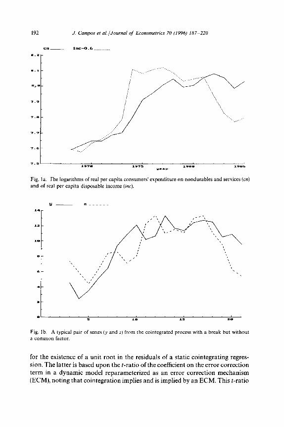
Before describing the test statistics in detail, it should be emphasized that either Case I or Case IV may characterize empirical time series, and it may be extremely difficult to distinguish between the two cases in practice. To illustrate, consider real per capita expenditure on nondurables and services (CN) and real per capita disposable income (ZNC) in Venezuela, graphed in logs in Fig. la as cn and inc. Initially, both series grow smoothly. Then, income jumps by over 30% in 1974 from increased petroleum revenues, remains relatively constant through 1981, and during the LDC debt crisis of the early 1980s falls to approximately its 1973 level. Expenditure parallels or lags behind income

J. Campos et al. JJournal of Econometrics 70 (1996) 187-220 191

through 1981, but falls only slightly during 1981-1985. Campos and Ericsson (1988) find that each series appears I(1) empirically, and that expenditure and income are cointegrated, provided that inflation and liquidity effects are properly accounted for.

Still, the expenditure and income series in Fig. la could easily have been

generated by a stationary process with breaks in 1974 and 1%. Fig. 1 b plots the series y and z generated by (lH4) under Case IV,’ and these series bear a marked resemblance to cn and inc in Fig. la. Yet, the power of a Dickey-Fuller

test to detect stationarity in such z, is less than its size; and the power of the Chow test to detect the break in z, is about 10% (at a nominal 5% level), even when the breakpoint is known. Such similarities in time series motivate the

Monte Carlo study below.

2.2. The test statistics

This subsection describes the test statistic for a unit root in the marginal process (2) and the test statistics for the cointegration of y, and z,.

2.2.1. Marginal processes

Frequently, investigators pre-test for unit roots in univariate autoregressive representations. Many tests exist: see Dickey and Fuller (1979, 1981), Phillips and Perron (1988), and Banerjee, Dolado, Galbraith, and Hendry (1993) inter

alia. While only the Dickey-Fuller t-statistic (denoted tDF) is considered in this paper, some of its properties are generic to unit root statistics. The asymptotic distribution of tDF is well-known for difference-stationary processes such as Case I. As shown in (15), its distribution is different when a break occurs.

2.2.2. Cointegrated processes

Using the dynamic bivariate process (lH4), this paper focuses on the relative

merits of the two-step Engle-Granger and single-step dynamic-model procedures for testing for the existence of cointegration. See Engle and Granger (1987) on the former and Banerjee, Dolado, Hendry, and Smith (1986) inter alia on the latter. The former is characterized by a Dickey-Fuller (DF) statistic used to test

‘Specifically, a = 0, b = - 0.1, p = 0.8, S = I, (TV = 6, = 1, T = 100, To = 25, and T, = 75. To

ensure comparable samples for Figs. la and 1 b, the Monte Carlo series y, and Z, were averaged over

four periods and selectively sampled, extracting every fourth (averaged) observation. Fig. 1 b plots observations 3 through 21 of the resulting series: breaks occur in observations 7 and 19. The graph of

the selectively sampled unaveraged series is similar to Fig. 1 b. Calculations for size and power use

the full sample (T = 100).

192 J. Campos et aLlJournal of Econometrics 70 (1996) 187-220

Fig. la. The logarithms of real per capita consumers’ expenditure on nondurables and services (cn)

and of real per capita disposable income (ix).

Fig. 1 b. A typical pair of series (y and z) from the cointegrated process with a break but without

a common factor.

for the existence of a unit root in the residuals of a static cointegrating regression. The latter is based upon the r-ratio of the coefficient on the error correction term in a dynamic model reparameterized as an error correction mechanism (ECM), noting that cointegration implies and is implied by an ECM. This r-ratio

J. Campos et aLlJournal of Econometrics 70 (1996) 187-220 193

is denoted the ECM statistic. Each statistic may utilize or ignore knowledge about the value of the cointegrating vector (i.e., that 1 = 1).2 This subsection describes these four test statistics and clarifies analytical relationships between the test statistics; Section 2.3 presents some of their asymptotic properties.

The variables y, and z, are cointegrated or not, depending upon whether b < 0 or b = 0. Thus, tests of cointegration rely upon some estimate of b. The four statistics considered here are all t-ratios on regression estimates of b. Let us denote those t-ratios by tECMk, tECMu, tDFk, and tDFu, where the subscripts ECM

and DF denote error correction model and Dickey-Fuller, and k and u indicate that the cointegrating vector is assumed known or unknown. These t-ratios on b are derived from the regressions:

dy, = K + adz, + b(y - z),- 1 + &,‘,,

Ay, = K + adz, + b(y - z),_~ + cz,el + E,*,

(5)

(6)

yt = IcO + z, + Wkt,

A(y - Izo - z)l = ~1 + b(y - co - z),-1 + e,c,,

and

y, = Kg + AZ, + Wut, (8)

A(y-i?o-~~)z),=~~ +b(y-IZo-I~),_l +e,,,

respectively, where K, K~, K~, and c are constants; and a tilde (*) denotes an estimate from the static regression in (7) or (8). The regression errors for

tECMk and tECMu are &k, and E,~, respectively. Those for tDFk and tDFu are ekt and e,,, with 6kt and 6,, being the associated static-regression residuals on which tDFk and tDFu are based.

The statistics tDFk and tEc& are used to test the null hypothesis that b = 0 in (l), i.e., that y and z are not cointegrated with a cointegrating vector (1: - 1). The statistics tDFu and tECMu g i nore that 1, = 1, and so are (implicitly or explicitly) used to test the null hypothesis that y and z are not cointegrated with an arbitrary cointegrating vector (1: - A).

Both asymptotic and finite-sample properties of the statistics can be better understood by examining the relationship between the DF regression equation (7) and the ECM regression equation (5). To do so, subtract dz, from both sides of the conditional DGP (1) and rearrange:

A(y - z), = b(y - z),pl + [(a - l)Az, + E,]

= b(y - z),- 1 + et, (9)

'A priori knowledge of the cointegrating vector frequently arises in economic modeling: for instance,

of (logs of) consumers’ expenditure and disposable income, of wages and prices, of money and

income, and of the exchange rate and foreign and domestic price levels.

194 J Campos et al./Journal of Econometrics 70 (1996) 187-220

where the disturbance e, is

e, = (a - l)dz, + E,. (10)

Eq. (7) is (9) with ek, = e, and an explicit constant term. The statistic tDFk ignores potential information contained in AZ,. Equivalently, (7) imposes the restriction

that the short- and long-run elasticities are equal (a = l), or that there is a common factor in the relationship between y, and z,.

For the DGP (l)(4), the error e, in (10) is white noise because both AZ, and

E, are white noise. Thus, the ADF, Z,, and Z, statistics offer no additional benefit in this case. The problem is the common factor restriction, which highlights the

difference between white noise and an innovation. As discussed in Kremers, Ericsson, and Dolado (1992) the ADF, Z,, and Z, statistics impose a common factor restriction.

A useful measure of the information ignored by tDFk is

q = - (a - l)s, (11)

where s = gJgE. That is, q2 is the variance of (a - l)Az, relative to that of E,. Also, q2 = @/( 1 - &), where %Y2 is the population R2 for A wkt (or e, in (10)) regressed on AZ, when b = 0. The value of q directly affects the distribution of

tECMk; see Section 2.3. See Kremers, Ericsson, and Dolado (1992) for details on the restriction a = 1, and Hendry and Mizon (1978) and Sargan (1964, 1980) on common factors.

The relationship between (8) and (6) (the regressions with unknown 2) paral-

lels that between (7) and (5). Eq. (1) can be transformed to

A(y - xz), = b(y - Iz)~_ 1

+ [(a - l)Az, + (1 - x)Az, + b(X- l)zl-t + at],

which is (8) where the disturbance e,, is

(12)

e,, = (a - l)Az, + (1 - ~Az, + b(I - l)z,_ 1 + Ed, (13)

and the constant in (12) is implicit. Thus, tDFu is affected not only by the common factor restriction, but also by the discrepancy between estimated and actual values of the cointegrating vector. While ‘super consistent’, the static-regression estimate 1 may have poor finite-sample properties, thereby affecting the properties of tDFu; see Banerjee, Dolado, Hendry, and Smith (1986).

2.3. Properties of the test statistics

This subsection describes properties of the test statistic for a unit root in the marginal process and properties of the cointegration test statistics.

J. Campos et al. /Journal of Econometrics 70 (1996) 187-220 195

2.3.1. Marginal processes Dickey and Fuller (1979, 1981) Phillips (1987b, 1988) and Banerjee, Dolado,

Galbraith, and Hendry (1993) derive the asymptotic distributions of tDF under Cases I and II; and they are identical to the distributions of tDFk, as described in Section 2.3.2 below. The Appendix derives properties of tDF under Case III, providing a baseline for interpreting the Monte Carlo results, which are for Case IV.

Under Case III, z, has a unit root (p = 1) and a break (6 # 0). Suppose an investigator, unaware of the break, estimates

AZ, = P + +-I + 5, (14)

in order to test for a unit root (4 = 0). The probability limit of the least squares estimator (p: $) of (cl: 4) is

= plim

1 iGK(K + 2M)

+dK(K + 2W I-’ [+;c2] &YK2(K + 3M)

=$H-’ 6K(M + K/6) 1 l-(K+2M) ’ (15)

where K is the length of the break (T, - T,)/T, M is the time after the break (T - T,)/T, and H = (1 - M - K)M + K(4 - 3K)/12. As found in additional Monte Carlo simulations not reported here, the estimated means of ,L and $ appear to match closely the analytical values in (15).

Four implications of (15) are of interest. First, the estimated intercept has a nonzero population value, which is proportional to 6. Second, the unit root estimator 3 + 1 differs from unity by only O,( T- ‘). Third, the corresponding discrepancy does not depend on 6 (to o,,(T- ‘)) and is relatively negligible, especially when (K + 2M) is close to unity. Fourth, a break in the marginal process (2) affects the cointegration statistic tDFk and the unit root statistic tDF for z, similarly when the common factor restriction is not valid for tDFk (a # 1).

196 J. Campos et al./Journal of Econometrics 70 (1996) 187-220

For tDFk, the equation being estimated is

d b - z)t = b(y - z)t- 1 + ekt

= b(y - z),- 1 + [(a - l)dz, + E,]

= b(y - z),-1 + [(a - 1)6D, + (a - 1) (p - 1) z,-1

+ (a - lb4 + 4, (16)

where the constant is implicit and the term in square brackets is the error. Under Case III, p = 1, so the error is comprised of a break (a - 1)6D, and white noise (a - l)u, + St, paralleling the regression (14) under the DGP (2) with p = 1 and 6 # 0. Under Case IV, 1 pi < 1, so the error also includes z,_ i, which has a break in it. Thus, whenever the marginal process has a break and the conditional process does not have a common factor, the regression for tDFk induces a break in the error, which may reduce the power of the corresponding cointegration test. By contrast, cointegration tests based on tECMk and tECMu do not suffer from this problem because their corresponding regressions are still properly specified.

2.3.2. Cointegrated processes Asymptotic distributions of all four cointegration test statistics are known for

Case I (z, with a unit root and no break), providing a baseline for the Monte Carlo study. Distributions under Cases II-IV are viewed as variants, with Case IV being the particular focus of Section 5. Because (l)(4) has a unit root under Case I, distributional results involve Wiener processes. That said, tECMk is approximately normally distributed for large q (when a # 1). Derivations of the asymptotic distributions appear in Dickey and Fuller (1979, 1981) and Phillips (1987b, 1988) (for tDFk); Banerjee, Dolado, Hendry, and Smith (1986) and Kremers, Ericsson, and Dolado (1992) (for tECMk ); Engle and Granger (1987) and Phillips and Ouliaris (1990) (for tDFu); and Park and Phillips (1988, 1989), Kiviet and Phillips (1992), Banerjee and Hendry (1992) Boswijk (1992) Banerjee, Dolado, Galbraith, and Hendry (1993), and this subsection (for tECMu).

For expositional convenience, we adopt certain notational conventions con- cerning Brownian motion (or Wiener) processes. Consider a normal, indepen- dently and identically distributed variable ylt, t = 1, . . . , T: that is, nt w IN(0, e,‘). Here, Q is usually either e,, St, or u,. Define BT,s(r) as the partial sum c\rrlnt/ ( To,~)“~, where I lies in [0, 11, and [ Tr] is the integer part of Tr. As discussed in Phillips (1987b), BT,q(r) converges weakly to a standardized Wiener process, denoted B,(r). For simplicity of notation, the argument r is suppressed, as is the range of integration over r when that range is [0, 11. Thus, integrals such as @,(r)2dr are written as J-B:. The symbol ‘a’ denotes weak convergence of the associated probability measures as the sample size T -+ CO. See Billingsley (1968)


and Banerjee, Dolado, Galbraith, and Hendry (1993) for further discussion. Derivations are presented below for cases without an intercept in the regression, for simplicity. When a constant term is included, the Brownian motions should be thought of as being ‘de-meaned’, corresponding to a prior regression that eliminates a constant. Mann and Wald’s (1943) order notation is used where needed.

The null hypothesis is no cointegration (b = 0). The alternative hypothesis is cointegration (b < 0), and is characterized as a local alternative with

b = eYiT - ~zJI/T, (17)

where y is a negative fixed scalar. Eq. (17) parallels the usual Pitman-type local alternative except that, in order to obtain statistics of O,(l), 6 differs from the null by O,(T- ‘) rather than by O,(T- 1’2). Conveniently, distributions under the null hypothesis are obtained by setting y = 0. The generalization of B,(r)

under this local alternative is the diffusion process:

K&) = j e(’ -“YdB,(j) 0

= B,,(r) + y j e’r-j)YB,Jj)dj, 0

(18)

where K,(r) is an implicit function of y; see Phillips (1987b). If y = 0, then K,(r) = B,(r). As with B,, the argument r in K,(r) and the limits of integration are dropped if no ambiguity arises from doing so.

Under the local alternative, tDFk is distributed as

which simplifies to the Dickey-Fuller distribution:

tDFk s B&w =-B: x/T

under the null hypothesis. Under the local alternative, the ECM statistic t&-Mk is distributed as

tECMk - ~(1 + q2)1’2( j K,2)“2

(19)

(20)

(a - 1) j K,dBe + s- 1 s K,dB,

+~~rr-1)2SKt+2(n-f)s-‘SK.K,+s-2SKT. (21)

198 J. Campos et al./.iournal of Econometrics 70 (1996) 187P220

When a = 1, (21) simplifies to the DF distributions (19) (for y # 0) and (20) (for y = 0).

For a # 1, (21) can be reparameterized in terms of y and q exclusively:

tEC&fk * y(l + qy ( 1 Ky + j K,d& - q - ’ s KdB,

,/JK,2 - 2q-‘[K,K, + q-‘SK:’ (22)

For large q, (22) is approximately a standardized normal distribution:

bXk = N(y(l + q*)l” ( s Ki)“‘, If + o&j- ‘), (23)

conditional on the process for u,. Under the null hypothesis, (23) simplifies to

&cMk =r N(O, 1) + G&Y-‘). (24)

The approximation in q is ‘small-e’ in nature; cf. Kadane (1970, 1971). Thus, as q varies from small to large, the asymptotic distribution of tEcMk shifts from the DF distribution to the normal distribution.

The asymptotic powers of tDrk and tE CMk are determined by (19) and (22). When q = 0, the two tests have the same power. When q is sufficiently large, tEcMk has (arbitrarily) greater power than t DFk. That discrepancy arises because tDFk is ignoring substantial information on A z,, whereas fEcMk uses that information to obtain a more precise estimate of b.

The asymptotic distributions of tDF,, and tECMu resemble those of tr,rk and tEcMk, but are somewhat more complicated because the hypothesized cointegrating vector is estimated. Phillips and Ouliaris (1990) derive the asymptotic distribution of tDFu under the null hypothesis that b = 0.

The test of b = 0 using tECMu is known to be similar when the conditioning variable z, is strongly exogenous for the regression parameters (a, b, c, CT:); see Kiviet and Phillips (1992), Banerjee and Hendry (1992) and Banerjee, Dolado, Galbraith, and Hendry (1993). The null limiting distribution of tEcMlr is implicit as a special case of Park and Phillips (1988, Thm. 4.la; 1989, Thm. 4.lb) and Boswijk (1992, Thm. 4.2, p. 85). The explicit representation provides insights not apparent from their general formulae, so it is derived here.

The DGP is (l)-(4) with b = 0 under Case I (i.e., with p = 1 and 6 = 0):

dy, = adz, + E,, E, - IN(0, d),

AZ, = tit, u, - IN(0, 0:). (25)

The estimated model is

Ay, = adz, + b(y - z),_ 1 + cz,_ , + v,,

which is (6) without a constant term.

(26)

J. Campos et aLlJournal of Econometrics 70 (1996) 187-220

The resealed parameter estimates from (26) are

i &a^ Tc^ - a) Tb

1 1 1

= T-312&-lur T-2i~;_ 1

1 1

w-l&-l

1 1

T-3~2t;z,_l~t T-2~w,-lz,_1 T-‘& 1 1 1 1

T-l&_le, 1

T-‘i~,_~c, 1

199

-1

(27)

where, from (25), w, is the random walk:

~,=y~-z~=w~-~+e~, (28)

and e, = (a - l)u, + E,, as in (10). Asymptotic distributions of the elements in (27) involve the Brownian motion processes B,, B,, and B,, where the last is related to the first two by

aeB, = aEBE + (a - l)a,B,.

Also, a: = a: + (a - 1)2ai. Hence, by partitioned inversion in (27):

(29)

T6aJjB”Z)(jBeW - (j&Be)(jBudBJ (Je (jB,2)(jB,2) - (jBAJ2 ’

Thus, the limiting distribution of tECMu is

tECMu * J&d& - (SB,B,)(SB,2)-l(SB,dB,)

JfB,” - ( j&BJ2@:)F1

= j&W - C j B,Bu) ( j B:)- ’ ( j Bud&)

JjBf - (jWu)2(jB;)-1 ’

(30)

(31)


using (29). Because the asymptotic distribution of tEcMu does not depend on a, cur or cE, it is invariant to those parameters, and hence tests based on tECMu are similar.

An alternative expression for (31) is enlightening. Consider the regression

Yt = Bz, + ir , (32)

‘linking’ the levels of J+ and z,. Let R denote the limiting form of Yule’s correlation for that regression when a = b = 0 (i.e., under the null of no relation between y, and z,) and that correlation is not adjusted for sample means. From Phillips (1986), R is

s R=Jgigiy (33)

Thus, schematically (31) is

lECMu * DF - R.N(O, 1)

JKE ’

where DF and N(0, 1) denote random variables with Dickey-Fuller and standardized normal distributions. This demonstrates that tECMu and the Dickey-Fuller statistic have different limiting distributions, so their critical values need separate tabulation. Also, (34) mirrors Park and Phillips’s (1988) Lemma 5.6, in which a related problem is addressed and R is a constant.

3. Experimental design and simulation

This section presents the experimental design and Monte Carlo simulation of the cointegration test statistics.

3. I. Experimental design

To analyze the size and power of the cointegration tests in the presence of a structural break, two sets of Monte Carlo experiments were conducted with (lH4) as the DGP. The first set is a ‘broad’ design, aimed at highlighting the effects of common factors, cointegration, and breaks over a range of sample sizes for estimation. The second set focuses on how the lack of a common factor affects the cointegration tests. Without loss of generality, a: = 1 and A = 1. Thus, the experimental design variables are the parameters (a, b, s, p, 6) (noting that s now is oU), the estimation sample size T,, the breakpoints To and T1, and the full sample size T.

J. Campos et al./Journal of Econometrics 70 (1996) 187-220 201

The first set of experiments is a full factorial design of

a = (1.0 [a common factor: 4 = 01, 0.0 [no common factor: 4 = s]),

b = (0.0 [no cointegration], - 0.1 [cointegration]),

s = 1.0.

p = (1.0 [integration], 0.8 [stationarity]),

6 = (0.0 [no break], 1.0 [a break of size s]),

T, = 10, 11, 12, . . . , T - 2, T - 1, T,

T, = 25, T, = 75, T=lOO,

(35)

resulting in 1456 experiments. For both sets of experiments, new z’s were generated for each replication, and the number of replications per experiment was P = 10,000.

The parameter values were chosen with the following in mind. For a = 1 (and so 4 = 0), the common factor restriction holds, so the distributions of the DF and ECM statistics should resemble each other. For a = 0, the common factor restriction is violated, but 4 = s = 1, which is a ‘moderately small’ value. The two values of b, 0.0 and - 0.1, imply lack of and existence of cointegration respectively, although, in the latter case, the corresponding root of the system is still large: 0.9. The root of the marginal process (p) is either unity or large but stationary. The break in the marginal process is either zero or unity (i.e., 1. CJJ, where the latter value is rather small by empirical standards. However, for the purposes of this paper, unity seemed appropriate because it is small enough to make its detection by standard Chow tests difficult.

The estimation sample size includes all integers in the interval [lo, 1001, providing small, medium, and large values. To ensure that most estimation sample sizes included a break, To = 25, with T1 = 75 so as to maximize the power of constancy tests over the full sample; see Hendry and Neale (1991). For a given length of break (T 1 - T,)/T, the particular choice of T,, and T 1 matters little for the power of the full-sample constancy tests.

While the generated data have two breaks, recursive testing allows examining estimation samples with zero breaks (T, < To), one ‘permanent’ break (To d T, < T 1), and two breaks (T, < T, d T). In this design, two breaks are equivalent to a single ‘temporary’ break. While the number of observations generated (T) and the estimation period (T,) are identical in the analytical derivations above, distinguishing between T and T, is necessary in recursive Monte Carlo. Below, the context clarifies whether ‘sample size’ means T or T,. Recursive testing also allows examining situations in which the break is at the very end of the estimation sample.

202 J. Campos et al. /Journal of Econometrics 70 (1996) 187-220

Critical values are all at the 5% level. For tDFk and tDFu, the values are calculated from MacKinnon’s (1991, Table 1) response surfaces with N = 1 and N = 2 respectively (Ma~Kinnon’s ‘N’), ‘with a constant but no trend’ for both. The correct critical values for t ECNk depend upon q as well as T,, and those for tEcMu depend upon T,. Both sets of critical values could be simulated. However, q may not be known in practice, and even asymptotic critical values for tECMu have not yet been simulated, so ‘safe’ critical values may be constructed by assuming that tECMk and tECMu have pure Dickey-Fuller-type distributions (i.e., q = 0). Thus, the critical values for tEcMk and tECMu used here are the same as those for tDFk and tDFu.

Because q is such an important parameter and because q G 1 in (35) is relatively small by empirical standards, the second set of experiments considers the effect of q = 3, albeit in a more limited design:

a = 0.0 [no common factor: q = s],

b = (0.0 [no cointegration], - 0.1 [cointegration]),

s = 3.0.

p = 0.8 [stationarity],

6 = 3.0 [a break of size s],

T, = 10, 11, 12, - . . . , T 2, T - 1, T,

To= 25, T1 = 75, T=lOO,

(36)

resulting in 182 experiments. The values of s and 6 are equal in order to keep the time series properties of z the same as in (35).

3.2. Simulation

Simulation proceeded as follows. Random numbers for a, and ut were generated by multiplicative congruential generators and transformed to a normal distribution by Box and Muller’s (1958) method. The first twenty observations of each replication from (l)-(4) were discarded in order to attenuate the effects of initial values in stationary relations (such as in yi - z, when b < 0). For a particular experiment, P replications were generated, with a statistic lying in its critical region S of P times (S dependent upon the statistic). The fraction of rejections S/P is an unbiased Monte Carlo estimate of the underlying rejection frequency (e.g., of size or power).

Recursive algorithms exist for the statistics tDFk, tECMk, and tECMu, providing a computationally efficient means for their calculation over the full range of sample sizes T, = 10, 11, . . . ,99, 100 for any given set of values of the other

J. Catnpos et al/Journal of Econometrics 70 (1996) 187-220 203

experimental design variables3 Thus, a replication of size T = 100 was generated, and the statistics were calculated recursively on that sample for all estimation sample sizes. Such re-use of the sample greatly reduces Monte Carlo variation for different values of T,; see Hammersley and Handscomb (1964). Further, calculation of all test statistics on the same sample reduces Monte Carlo variation for the differences in properties across statistics. Graphical (rather than tabular) analysis of the Monte Carlo rejection frequencies is highly desirable, given the large number of experiments; cf. Ericsson (1991). Graphical analysis also corresponds to a (pseudo-) nonparametric estimation of the size and power functions of the tests.

4. Post-simulation analysis: The marginal process

This section briefly examines one unit-root test statistic and two constancy test statistics on the marginal process for z,. The unit root statistic is the Dickey-Fuller statistic with a constant term (tDF), which is the t-ratio on 4 in (14), noting that the break dummy D, is explicitly excluded. The first constancy statistic is Chow’s (1960) predictive failure statistic applied to (14) and is denoted F CHOW. The second constancy statistic is the t-ratio on the least squares estimate of 6 in the correctly specified marginal process (albeit with a constant term estimated):

AZ, = p + $z,- t + 6D, + ut, (37)

and is denoted td. This last statistic is also a statistic for testing the invariance of (14) to D,, as discussed in Engle and Hendry (1993). Critical values are at the 5% level and are taken from MacKinnon (1991) for tDF, the F distribution for

FCHOW and the t distribution for ts. Figs. 2a, 2b, and 2c plot the estimated rejection frequencies of tDF, FCHOW, and

td, respectively. The four lines on each graph correspond to Case I (p = 1, 6 = 0: -), Case II (p = 0.8, 6 = 0: - -), Case III (p = 1, 6 = 1: ......), and Case IV (p = 0.8, 6 = 1: - - -).

From Fig. 2a, the estimated size of tDF (Case I) is close to 5% for all sample sizes. When p = 0.8 without a break (Case II), the power increases monotoni- cally from about 7% (at T, = 10) to 90% (at T, = 100). When a break is added to that stationary series (Case IV), the power falls from 13% at T, = 25 to less than 1% by T, = 40, increasing to only around 2+% by T, = 100. As examined

‘The statistic tDF, cannot be calculated recursively, so its properties are considered for T, = 100

only. Also, D, was perturbed by a small error in order to permit recursive estimation for T, Q 25 of

equations including D,.

204 J. Campos et al. /Journal of Econometrics 70 (1996) 187-220

I II.__-- I I I IU _._~ _....

1e.o

se

BO

i TO

t dZ

,

0 .... t0 JO 19 50 1 co

Fig. 2a. Estimated rejection frequencies of t DF for the marginal process (Cases I-IV).

I II.____ I I I IV _ ..____.

109

99

ao

i

Fig. 2b. Estimated rejection frequencies of the split-sample F CHOW (NJ) for the marginal process

(Cases I-IV).

in greater detail by Hendry and Neale (1991), even small breaks can dramatically reduce the power of unit root tests. The size is also affected by breaks, noting that the rejection frequency for Case III varies between 0% and 25%, depending upon what fraction of the sample includes the break.


PO- \

xe- _-__------_________

__----__ _-_-_---_---__

0 ...“.. 10 30 .#a 59 r == 7-e em 99 1-o

Fig. 2c. Estimated rejection frequencies of the invariance statistic td for the marginal process (Cases

I-IV).

From Fig. 2b, the estimated size of F cHOW (Cases I and II) is about 7%-9% for small samples, tending to its nominal 5% value by T, = 100. For stationary z, with a break, the power is never higher than 12%, even for a sample split at T, = 25 where the first break occurs. The power is somewhat higher for nonstationary z,, but still never exceeds 30%. In essence, a break of one standard deviation over half the sample is small and hard to detect, in spite of its consequences for the unit root test.

The statistic td should provide a highly powerful test, given that the dates and nature of the break are treated as known. However, controlling its size is problematic, as Fig. 2c documents. Intuitively, D, behaves like an integrated process and so the distribution of td is affected by the correlation between z,_r and D, in (37). This effect is lessened but not eliminated when z, has a stationary root.4 The ‘power’ of td appears impressive, but must be treated with caution, given the large distortion to size.

To summarize, the break in the marginal process is difficult to detect with the Chow statistic, yet it dramatically reduces the power of the Dickey-Fuller statistic for detecting a stationary root. A stationary process with a break is virtually observationally equivalent to a unit root process with no break.’

4Note, however, that if the root of .z, were treated as known, the distribution of td would be exactly

a t.

‘Faust (1993) formally establishes the near observational equivalence of trend-stationary and

difference-stationary processes. His framework also may help establish a parallel result here.

206 J. Campos et al.lJournal of Econometrics 70 (1996) 187-220

5. Post-simulation analysis: Tests of cointegration

This section examines the cointegration statistics (tECMb tDFk, tECMu, tDFu) as defined by (5HS). Rejection frequencies are the primary focus, but means, standard deviations, and overall distributional properties are also considered.

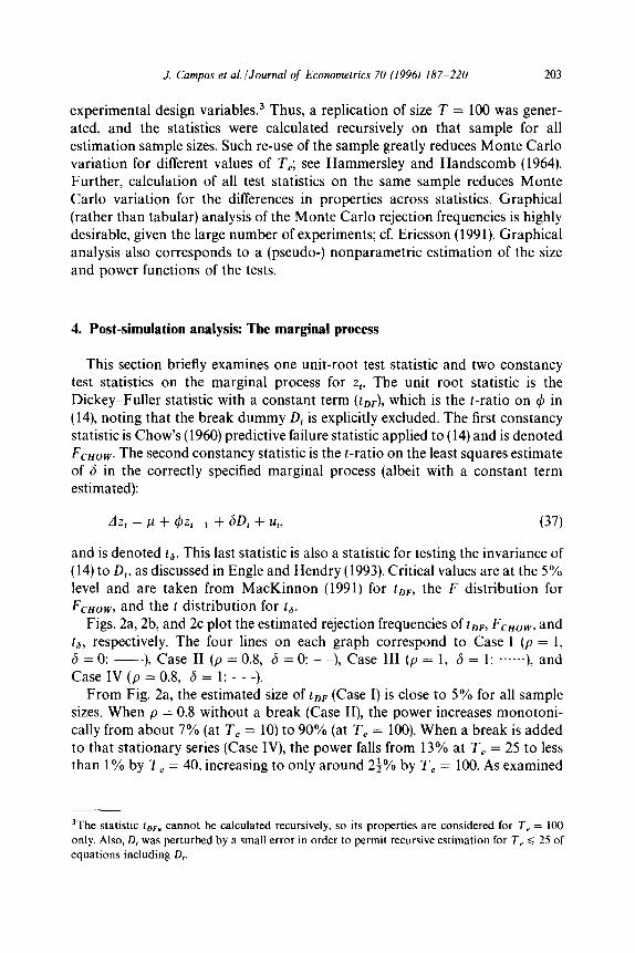
Figs. 3 and 4 plot rejection frequencies by the four cointegration tests for the first set of experiments. These rejection frequencies are under the hypotheses of no cointegration (Fig. 3) and cointegration (Fig. 4), and correspond to size and power, provided the correct critical values are used. Figs. 3a-3d plot estimated sizes for (a = 1, 6 = 0), (a = 1, 6 = l), (a = 0, 6 = 0), and (a = 0, 6 = l), respectively: that is, for DGPs with and without a common factor in the conditional process and with and without a break in the marginal process. Figs. 4aa4d present the corresponding plots for estimated powers. The primary interest here is in discerning the differences between Cases I and IV, so p = 1 when 6 = 0 and p = 0.8 when 6 = 1.

From Figs. 3a and 3b, the estimated sizes for tECMk and tDFk are both approximately 5%, which follows from the asymptotic equivalence of the two statistics when there is a common factor (a = 1). The size of tECMu is around 3% because of the conservative choice of using MacKinnon’s critical values. All three sizes are virtually unaffected by the sample size T,, confirming the accuracy of MacKinnon’s response surfaces for the critical values. The estimated size of tDFu is available at only T, = 100, and is approximately 5%.

Invalidity of the common factor restriction (Figs. 3c and 3d) clearly affects

tEC!Mk and tDFk. As anticipated from the asymptotics with no break, the rejection frequencies for tECMk are below 5% (typically, between 2% and 4%), while those

for &Mu are unchanged (at 3%) from simulations with a common factor. The rejection frequency of tDFk is about 5% in Fig. 3c, in line with its invariance to the existence or lack of a common factor when there is no break; cf. Kremers, Ericsson, and Dolado (1992). However, its rejection frequency is not invariant to the lack of a common factor when there is a break. The residual in the estimated equation for tDFk involves dz,, which includes D, and a stationary error: see (9). The average size for tDFk is about 6f% which is substantially higher than the sizes for tECMk and tECMu.

Clearly, both the DF and ECM tests are less than perfect. However, noting that the actual size is defined as the maximum rejection frequency over the parameter space for the null hypothesis, the ECM tests at least control for size whereas the DF test does not. Also, because t ECMu appears invariant to the break and is invariant to a, better critical values for it are easily calculated by Monte Carlo. When there is no common factor, tDFk is not invariant to the break (see Fig. 3d), so useful critical values for tDFk are problematic to obtain. That lack of invariance is even more apparent for powers and for larger 4, as seen below.

In Figs. 4a and 4b, the DGP has a common factor, and y, and z, are cointegrated. As under the null of no cointegration, the presence or lack of


a break has no effect on the test statistics; and the estimated powers for tDFk and tECMk are virtually identical, ranging from 5% at T, = 10 to 33% at T, = 100. The rejection frequency of tECMu is somewhat less, and unsurprisingly so because its rejection frequency under the null is less than 5% and because it ignores 1 being unity.

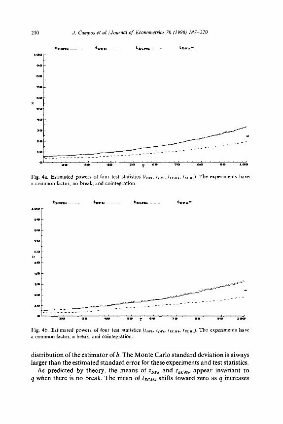
When there is no common factor and no break (Fig. 4c), the power of tECMk substantially dominates that of tDFk, with the former increasing to 70% by T, = 100. Even tECMu does better than tDFk at moderate to large samples, in spite of ignoring the value of the cointegrating vector. In fact, the power of tDFk is invariant across Figs. 4a, 4b, and 4c. By contrast, the powers of tECMk and tECMu increase when the common factor is invalid, as predicted by theory.

With a break but no common factor (Fig. 4d), the power of tECMk exceeds that

Of tDFk except for very small samples, where both powers appear approximately equal to size. Discrepancies between their powers at larger sample sizes appear smaller than without a break, but this is probably a spurious result due to inadequate control of the rejection frequency of tDFk under the null hypothesis (see Fig. 3d).

Figs. 5a and 5b plot estimated sizes and powers for the second set of experiments. The DGP has no common factor and a large break (6 = 3) so these figures are qualitatively similar to Figs, 3d and 4d, but effects of the break are more pronounced from having a larger q. The rejection frequency of tECMk in Fig. 5a is even smaller than in Fig. 3d, as predicted by the asymptotic distribution of tECMk shifting towards a normal distribution as q increases. Rejection frequencies for tDFk resemble those in Fig. 3d, but with a larger range, 2%-l 1%. The distribution of tECMu still appears invariant to the break.

Because of the greater information content in dz,, the powers for tECMk and tECMu in Fig. 5b increase more rapidly with T, than their powers in Fig. 4d do. The ‘power’ of tDFk has more pronounced dips after the breaks occur than in Fig. 4d, and is somewhat inflated because its rejection frequency under the null hypothesis is inadequately controlled. Even so, the power of tECMk dominates that of tDFk for all sample sizes, as does the power of tECMu for T, > 40. By contrast, the power of tDFu is less than its size at T, = 100. Figs. 4d and 5b also show how a test’s power may either increase (tECMk and tECMu) or decrease (tDFk) when the estimation sample is lengthened to include the first observation of a break.

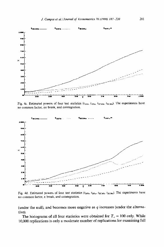
Table 1 summarizes the results in Figs. 335 by listing the approximate values or (where appropriate) ranges of rejection frequencies for all four tests under the various parameterizations: with and without a common factor (a = 1 and a = 0); and with no break (6 = 0), a small break (6 = l), and a large break (6 = 3). With a common factor, DF and ECM tests perform similarly. Without a common factor, ECM tests are preferred, having higher power and better control of size.

Campos, Ericsson, and Hendry (1993, App. B) examine other distributional aspects of the cointegration test statistics, graphing their histograms, their

208 J. Campos et al. jJourna1 of Econometrics 70 (1996) 187-220

Fig. 3a. Estimated sizes of four test statistics (t Wli, tDFu, tECMk, tECMu). The experiments have a common factor, no break, and no cointegration.

-a- * ,_--,-cl _“__C_.

<- I h_

\

3- c-*._ _%_.’ --*-._ c__--c_,____

-...\ ,e’.

8-

+-

0 ‘.. ‘~‘~~~‘.~~~‘.‘.~..~~‘~.. *..‘- 8’ “I .‘.I PO am 19 JO r 69 70 89 9Q toe

Fig. 3b. Estimated sizes of four test statistics (t Dplr, tDFu, tEcm, tBcMu). The experiments have a common factor, a break, and no cointegration.

means, and the means of the corresponding estimated coefficients. With the exception of the means of the statistics themselves, there is little to distinguish the properties of the test statistics across DGPs (e.g., with or without a break) and even across test statistics for a given DGP.


x 1 . .

5 . . . .,, ..” ,...’ _..; ..: ..: .. .a i . . .._.. ../’ ..’

I-

>__,\,

*_-_-_-_

-

P-

0 ‘....- .‘. ...L.‘..n 19 90 .o 19 r 60 ?#a 89 90 S.-e

Fig. 3c. Estimated sizes of four test statistics (tDFII, tDFu, tEcMII, tEcMu). The experiments have no common factor, no break, and no cointegration.

t,crr* - torr .._ ~lccmu - - - tImA* 29

F

01 29 99 19 50 T 60 70 eo 99 I.99

Fig. 3d. Estimated sizes of four test statistics (tDFk, tDFu, tECMkr tECMu). The experiments have no common factor, a break, and no cointegration.

For each test statistic and DGP, the recursively estimated Monte Carlo mean of the estimate of b is calculated with plus-or-minus twice its (average) estimated standard error, as would be computed by a regression package, and plus-or- minus twice the Monte Carlo standard deviation, reflecting the actual sampling


39-

ao-

__--- +e- _____a--

____-----

,I-..-~~~~.~~ ..““.‘.‘.““‘.“...’ .“‘...‘I 19 19 40 JO 1 LO 78 88 se *am

Fig. 4a. Estimated powers of four test statistics (t DFlrr tDFU, tECMt, tECMu). The experiments have a common factor, no break, and cointegration.

Fig. 4b. Estimated powers of four test statistics (tDFt, tDFvr tECMX, tECMu). The experiments have

a common factor, a break, and cointegration.

distribution of the estimator of b. The Monte Carlo standard deviation is always larger than the estimated standard error for these experiments and test statistics.

As predicted by theory, the means of tDFk and tECMu appear invariant to q when there is no break. The mean of t ECMk shifts toward zero as q increases


28- _..__.<. -.c ..

.,... - _ r ..... ......

________------

______----

0 ‘...‘- ..t.. “‘...‘..- ” ae se ID 50 T LB 79 eo se 188

Fig. 4c. Estimated powers of four test statistics (tDFk, tDFur tECMkr tECMu). The experiments have no common factor, no break, and cointegration.

-?8-

68-

% -

JO-

-e-

,#a-

ze- _--/ __--

__-- ___----

-___________-- 0 ~.~~~-~~~~~~~~~~~‘~~~‘~~~’

PB 30 .D =I0 T 68 79 80 S-0 loe

Fig. 4d. Estimated powers of four test statistics (tDFk, tDFu, tEcMk, tECMu). The experiments have no common factor, a break, and cointegration.

(under the null), and becomes more negative as q increases (under the alternative).

The histograms of all four statistics were obtained for T, = 100 only. While 10,000 replications is only a moderate number of replications for examining full

212 J. Campos et al.l.Iournal of Econometrics 70 (1996) 187-220

Fig. 5a. Estimated sizes of four test statistics (tDFI, tDFur tECMk, fECMu). The experiments have no common factor, a large break (6 = 3), and no cointegration.

Fig. 5b. Estimated powers of four test statistics (tDFkr tDFu, tECMk, tECMu). The experiments have no common factor, a large break (6 = 3), and cointegration.

distributional properties of the statistics, their distributions overall appear normal, in line with Banerjee and Dolado’s (1988) result that the Dickey-Fuller distribution is well approximated by a normal distribution with a negative mean.

.J. Campos et al. /Journal of Econometrics 70 (1996) 187-220

Table 1 Estimated rejection frequencies for cointegration tests

213

Fig. a 6 tDFk tECMk CDF” km

Size

3a 1 0 5.0 5.0 5.0 3.5 3b 1 1 5.0 4.9 4.1 3.2 3c 0 0 5.1 2.6 4.8 3.3 3d 0 1 [4.6, 7.41 2.9 4.3 3.1 5a 0 3 c2.0, 10.81 1.1 4.5 3.1

Power

4a 1 0 C5.5, 33.21 [5.8, 32.71 22.8 [3.9, 19.21 4b 1 1 [5.1, 33.51 [5.2, 32.41 22.2 [3.2, 18.31 4c 0 0 c5.3, 33.71 [5.7, 70.71 14.6 [3.4, 40.43 4d 0 1 [6.1, 45.41 C5.5, 68.71 15.5 [3.2, 34.81 5b 0 3 C6.8, 55.31 C8.4, 99.91 2.9 [2.8, 98.11

Single values are means; values in square brackets indicate the range over 7,; all values are percentages. The size and power for t,,, were estimated for T, = 100 only.

While the Monte Carlo study in this paper is limited by a relatively small experimental design for a, s, and b, both asymptotic theory and these simulations point to the advantages of the ECM statistics for empirically common values of a and s. Control of size appears relatively straightforward for the ECM statistics in the presence of breaks. Tests with tECMu are insensitive to breaks under the null hypothesis, and MacKinnon’s Dickey-Fuller critical values provide a ‘safe’ choice for tECMk and tECMw Further, the power of the ECM statistics commonly exceeds that of DF statistics for empirically interesting parameter values.

Recursive algorithms helped reduce Monte Carlo imprecision across statistics and across (econometric) estimation sample sizes, with graphical analysis providing a clear, simple summary of a vast array of estimated sizes and powers. Recursive procedures are also appealing empirically. Because statistics are affected by the accrual of information over time, full-sample and partial-sample inferences may differ, especially with breaks. Recursive estimation and testing offer a window on those effects.

6. Summary and remarks

Testing for cointegration has become an important facet of the empirical analysis of economic time series. Various tests have been proposed and widely

214 J. Campos et al/Journal of Econometrics 70 (1996) 187-220

applied, but most distributional results rest on the assumption of unit root processes with no structural breaks. Even so, regime shifts and structural breaks are empirically and economically plausible, as indicated by extensive discussion of the Lucas (1976) critique. Using Monte Carlo methodology, this paper examines the finite-sample properties of four common tests of cointegration in the presence of a structural break.

When conditioning is valid, Dickey-Fuller statistics used to test for cointegration have no particular advantage over their ECM counterparts; and there is much to gain from using the latter when the common factor restriction is invalid, and especially so if a break occurs as well. These differences arise because the DF statistic ignores potentially valuable information by imposing a possibly invalid common factor restriction. Because common factor restrictions are generic to univariate-based tests of cointegration, these results should hold for the augmented Dickey-Fuller statistic, Sargan and Bhargava’s (1983) statistic, Phillips’s (1987a) 2, and 2, statistics, and generalizations thereon by Phillips and Perron (1988) and Gregory and Hansen (1996). The problem is in using these univariate- based statistics to test a multivariate hypothesis, and not in the statistics themselves.

Conversely, maximum likelihood procedures such as those developed by Johansen (1988, 1991, 1992a), Johansen and Juselius (1990) Phillips (1991), and Boswijk (1992) do not impose common factor restrictions and so can have more desirable properties. Some caveats apply in practice. First, systems procedures may require modeling the break itself, and that may be difficult. Second, while conditional modeling is often simpler than dealing with complete systems, the assumed weak exogeneity may be invalid, implying trade-offs between conditional modeling and systems modeling. Third, even in conditional models, general dynamics may not be sufficient to account for breaks. If breaks occur in the cointegrating vector itself, the Lagrange multiplier statistic of Quintos and Phillips (1993) may help detect them. With or without breaks anywhere in the DGP, properly accounting for the dynamic relationship between variables can be critical in testing for a long-run relationship between them.

Appendix: Breaks and the distribution of the unit root estimator

This Appendix derives asymptotic properties of the unit root estimator when the underlying process has a break. The asymptotic distribution of tDFk with no break was solved by Dickey and Fuller (1979).

Consider the DGP for zt in (2) under Case III:

AZ, = 6D, + u,, ut - IN@, d), (A.11

where z,, = 0. Let K, L, and M be the length of the break (T, - T,)/T, the time until the end of the break TJT, and the time after the break 1 - L, respectively,

J. Campos et al./.lournal of Econometrics 70 (1996) 187-220 215

all relative to the time period T. An investigator, unaware of the break, estimates

&=~+4z,-~+L (A.21

in order to test for a unit root (4 = 0). This section derives large-sample properties of

(A.3)

the least squares estimator of (P:c$) in (A.2), when (A.l) holds for fixed nonzero 6 and K. Here and below, summations are over t unless otherwise indicated.

Evaluation of the four different summations in (A.3) is required. Without loss of generality, set a,2 = 1, so 6 is measured in standard deviations of u,. Also, all summations utilize an explicit representation for z,:

Z, = i Azj = 6 i Dj + i Uj = 61, + ht, j= 1 j=l j=t

(A.4)

where

I,= t-T, I 0 if t = 1, . . . , To,

if t=T,+l,...,T,,

TK if t = T1 + 1, . . , T,

and

h, = i Uj, t = 1, ...) T, j= 1

(A.5)

64.6)

with h, being a random walk. Evaluating (A.4) at t = T obtains the summation CTAz,:

iAz,=z7=dTK+hT, 1

OJTI O,(T”‘)

(A.7)

where orders of magnitude appear below the component terms in the last line. While terms such as 6TK are nonstochastic, it is convenient (and legitimate) to use probabilistic orders throughout.

216 J. Campos et al/Journal of Econometrics 70 (1996) 187-220

The summation cTzt_ 1 is (c rzt) - zT + zo, where CTz, can be obtained by using (A.4) and evaluating the summation of I, over the three subsamples:

gzt = $4 1 + ih, 1

=o+s 5 I,+6 f: I,+ih, To+ 1 T, + 1 1

=s 2 (t-T,)+6 i TK+?h, To+1 T, + 1 1

TK TM 7

=SCj+SCTK+xh, j=l j= 1 1

T

=f6T2K[(K+T-‘)+2M]+xh, 1

= &ST ‘K[K + 2M-J + i h, + O,(T). 1

O,V’) 0 (T”‘) P

(‘4.8)

Because zT is O,,(T) and z. = 0, the summation cFzt_ 1 is (A.8) to O,(T). The summation cTz:_ 1 is obtained in a similar fashion.

TK TM

= 4d2T3K2[K + 3M] + 26 1 jhT,+j + TK 1 hT,+j + 0,(T2). O,V’) j=l (7 5.q j=l 1 0 &- 64.9)

Because z$ is 0,(T2), the summation 1; z:- 1 is (A.9) to O,(T 2). Noting (A.l), the summation cTzt- 1 AZ, is obtained by evaluating each of the

summations 1 Tzt _ 1 u, and 1 rzt _ 1 D,:

~z,-,u~=~~l,-,u,+i;h,~,u, 1 1

EjUyO+ji-TKTfUT,+j +~h,_1u,+0,(T”2), (A.10) j=l

0 (T”‘) j=l 1 1

I O,(T)


and

@_,D* = 6&D, + ih,_,D, 1 1

TK TK

=6 cj+ 1 hTo+j-l +OptT)

j=l j= 1

=f6T2K2 + F hT,+j_l + O,(T). j=l

OJT’) 0 0 (T “‘)

(A.1 1)

From (A.lO) and (A.ll) it follows that

=+d2T2K2+6 T,+j-1 +.bT,+j) + TK ‘f uT,+j

WT2) 0 (T”‘“) j=l 1 I

+ O,(T). (A.12)

The probability limit of (A.3) can now be evaluated. Pre-multiplying (A.3) by

1 0

[ 1 0 T

and substituting (A.7), (A.8), (A.9), and (A.12) into that equation obtains (15) in the text. The limiting distribution of (A.3) is somewhat complicated. Because (jI: T$) has a nonzero plim, the stochastic components of the first as well as the second matrix on the right-hand side of (A.3) must be taken into account. We plan to derive that limiting distribution in due course.

References

Banerjee, A. and J.J. Dolado, 1988, Tests of the life cycle-permanent income hypothesis in the

presence of random walks: Asymptotic theory and small-sample interpretations, Oxford Eco-

nomic Papers 40, 61&633. Banerjee, A. and D.F. Hendry, 1992, Testing integration and cointegration: An overview, Oxford

Bulletin of Economics and Statistics 54, 2255255. Banerjee, A., J.J. Dolado, J.W. Galbraith, and D.F. Hendry, 1993, Co-integration, error correction,

and the econometric analysis of non-stationary data (Oxford University Press, Oxford). Banerjee, A., J.J. Dolado, D.F. Hendry, and G.W. Smith, 1986, Exploring equilibrium relationships

in econometrics through static models: Some Monte Carlo evidence, Oxford Bulletin of Eco-

nomics and Statistics 48, 2533277.

218 J. Campos et al. JJournal of Econometrics 70 (1996) 1877220

Billingsley, P., 1968, Convergence of probability measures (Wiley, New York, NY).

Boswijk, H.P., 1992, Cointegration, identification, and exogeneity, Research series no. 37 (Tinbergen

Institute, Amsterdam).

Box, G.E.P. and M.E. Muller, 1958, A note on the generation of random normal deviates, Annals of

Mathematical Statistics 29, 61@611.

Campos, J. and N.R. Ericsson, 1988, Econometric modeling of consumers’expenditure in Venezuela,

International finance discussion paper no. 325 (Board of Governors of the Federal Reserve

System, Washington, DC).

Campos, J., N.R. Ericsson, and D.F. Hendry, 1993, Cointegration tests in the presence of structural

breaks, International finance discussion paper no. 440 (Board of Governors of the Federal

Reserve System, Washington, DC).

Chow, G.C., 1960, Tests of equality between sets of coefficients in two linear regressions, Econo-

metrica 28, 591-605.

Davidson, J.E.H. and D.F. Hendry, 1981, Interpreting econometric evidence: The behaviour of

consumers’ expenditure in the UK, European Economic Review 16, 177-192.

Davidson, J.E.H., D.F. Hendry, F. Srba, and S. Yeo, 1978, Econometric modelling of the aggregate

time-series relationship between consumers’ expenditure and income in the United Kingdom,

Economic Journal 88, 661-692.

Dickey, D.A. and W.A. Fuller, 1979, Distribution of the estimators for autoregressive time series

with a unit root, Journal of the American Statistical Association 74, 427431.

Dickey, D.A. and W.A. Fuller, 1981, Likelihood ratio statistics for a&regressive time series with

a unit root, Econometrica 49, 1057-1072.

Doornik, J.A. and D.F. Hendry, 1992, PcGive version 7: An interactive econometric modelling

system, Version 7.00 (Institute of Economics and Statistics, University of Oxford, Oxford).

Engle, R.F. and C.W.J. Granger, 1987, Co-integration and error correction: Representation, estima-

tion, and testing, Econometrica 55, 251-276.

Engle, R.F. and D.F. Hendry, 1993, Testing super exogeneity and invariance in regression models,

Journal of Econometrics 56, 119-139.

Engle, R.F., D.F. Hendry, and J.-F. Richard, 1983, Exogeneity, Econometrica 51, 277-304.

Ericsson, N.R., 1991, Monte Carlo methodology and the finite sample properties of instrumental

variables statistics for testing nested and non-nested hypotheses, Econometrica 59, 124991277.

Faust, J., 1993, Near observational equivalence and unit root processes: Formal concepts and

implications, International finance discussion paper no. 447 (Board of Governors of the Federal

Reserve System, Washington, DC).

Gregory, A.W. and B.E. Hansen, 1996, Residual-based tests for cointegration in models with regime

shifts, Journal of Econometrics 70, this issue.

Hammersley, J.M. and D.C. Handscomb, 1964, Monte Carlo methods (Chapman and Hall, London).

Hendry, D.F., 1984, Monte Carlo experimentation in econometrics, Ch. 16 in: Z. Griliches and

M.D. Intriligator, eds., Handbook of econometrics, Vol. 2 (North-Holland, Amsterdam)

9377976.

Hendry, D.F. and G.E. Mizon, 1978, Serial correlation as a convenient simplification, not a nui-

sance: A comment on a study of the demand for money by the Bank of England, Economic Journal 88, 5499563.

Hendry, D.F. and A.J. Neale, 1987, Monte Carlo experimentation using PC-NAIVE, in: T.B. Fomby

and G.F. Rhodes, Jr., eds., Advances in econometrics, Vol. 6 (JAI Press, Greenwich, CT) 91-125.

Hendry, D.F. and A.J. Neale, 1990, PC-NAIVE: An interactive program for Monte Carlo experi-

mentation in econometrics, Version 6.01 (Institute of Economics and Statistics and Nuffield College, University of Oxford, Oxford), documentation by D.F. Hendry, A.J. Neale, and N.R. Ericsson.


Hendry, D.F. and A.J. Neale, 1991, A Monte Carlo study of the effects of structural breaks on tests for unit roots, Ch. 8 in: P.Hackl and A.H. Westlund, eds., Economic structural change: Analysis and forecasting (Springer-Verlag, Berlin) 95-l 19.

Johansen, S., 1988, Statistical analysis of cointegration vectors, Journal of Economic Dynamics and Control 12, 231-254.

Johansen, S., 1991, Estimation and hypothesis testing of cointegration vectors in Gaussian vector autoregressive models, Econometrica 59, 1551-1580.

Johansen, S., 1992a, Cointegration in partial systems and the efficiency of single-equation analysis, Journal of Econometrics 52, 389402.

Johansen, S., 1992b, A representation of vector autoregressive processes integrated of order 2, Econometric Theory 8, 188-202.

Johansen, S., 1992c, Testing weak exogeneity and the order of cointegration in UK money demand data, Journal of Policy Modeling 14, 313-334.

Johansen, S. and K. Juselius, 1990, Maximum likelihood estimation and inference on cointegration - With applications to the demand for money, Oxford Bulletin of Economics and Statistics 52, 169-210.

Kadane, J.B., 1970, Testing overidentifying restrictions when the disturbances are small, Journal of the American Statistical Association 65, 182-185.

Kadane, J.B., 1971, Comparison of k-class estimators when the disturbances are small, Econo- metrica 39, 723-737.

Kiviet, J.F. and G.D.A. Phillips, 1992, Exact similar tests for unit roots and cointegration, Oxford Bulletin of Economics and Statistics 54, 349-367.

Kremers, J.J.M., N.R. Ericsson, and J.J. Dolado, 1992, The power of cointegration tests, Oxford Bulletin of Economics and Statistics 54, 3255348.

Lucas, Jr., R.E., 1976, Econometric policy evaluation: A critique, in: K. Brunner and A.H. Meltzer, eds., Carnegie-Rochester conference series on public policy, Vol. 1 (North-Holland, Amsterdam) 1946.

MacKinnon, J.G., 1991, Critical values for cointegration tests, Ch. 13 in: R.F. Engle and C.W.J. Granger, eds., Long-run economic relationships: Readings in cointegration (Oxford University Press, Oxford) 267-276.

Mann, H.B. and A. Wald, 1943, On stochastic limit and order relationships, Annals of Mathematical Statistics 14, 217-226.

Park, J.Y. and P.C.B. Phillips, 1988, Statistical inference in regressions with integrated processes: Part 1, Econometric Theory 4, 468-497.

Park, J.Y. and P.C.B. Phillips, 1989, Statistical inference in regressions with integrated processes: Part 2, Econometric Theory 5, 955131.

Perron, P., 1989, The great crash, the oil price shock, and the unit root hypothesis, Econometrica 57, 1361~1401.

Phillips, P.C.B., 1986, Understanding spurious regressions in econometrics, Journal of Econometrics 33, 31 l-340.

Phillips, P.C.B., 1987a, Time series regression with a unit root, Econometrica 55, 277-301. Phillips, P.C.B., 1987b, Towards a unified asymptotic theory for autoregression, Biomettika 74,

5355547. Phillips, P.C.B., 1988, Regression theory for near-integrated time series, Econometrica 56,

1021-1043. Phillips, P.C.B., 1991, Optimal inference in cointegrated systems, Econometrica 59, 283-306. Phillips, P.C.B. and S. Ouliaris, 1990, Asymptotic properties of residual based tests for cointegration,

Econometrica 58, 1655193. Phillips, P.C.B. and P. Perron, 1988, Testing for a unit toot in time series regression, Biometrika 75,

3355346.

220 J; Campos et d/Journal of Econometrics 70 (19963 187-220

Quintos, C.E. and P.C.B. Phillips, 1993, Parameter constancy in cointegrating regressions, Empiri- cal Economics 18, 675-706.

Sargan, J.D., 1964, Wages and prices in the United Kingdom: A study in econometric methodology, in: P.E. Hart, G. Mills, and J.K. Whitaker, eds., Econometric analysis for national economic planning, Colston papers, Vol. 16 (Butterworths, London) 25-63 (with discussion); reprinted in D.F. Hendry and K.F. Wallis, eds., 1984, Econometrics and quantitative economics (Basil Blackwell, Oxford) 275-3 14.

Sargan, J.D., 1980, Some tests of dynamic specification for a single equation, Econometrica 48, 879-897.

Sargan, J.D. and A. Bhargava, 1983, Testing residuals from least squares regression for being generated by the Gaussian random walk, Econometrica 51, 153-174.

cointegration tests in the presence of structural breaks

Documents