cold plasma dispersion surfaces - repository home

J. Plasma Physics (1979), vol. 21, part 2, pp. 205-224 205Printed in Great Britain

Cold plasma dispersion surfaces

By M. E. OAKES, R. B. MICHIE, K. H. TSUIDepartment of Physics, The University of Texas, Austin, Texas 78712

AND J. E. COPELANDDepartment of Physics, Southwestern University,

Georgetown, Texas 78726

(Received 5 July 1978)

Three-dimensional plots of dispersion in a cold anisotropic plasma are presented.The d)(k, 0) surfaces provide a clear picture of the behaviour of cold plasmawaves as the direction of propagation is varied. The group velocity (do)/dk)has a simple geometrical interpretation on the surfaces.

1. IntroductionIn Stix's (1962) excellent book on plasma waves, he presented the theory of

cold plasma waves using a diagram first proposed by Clemmow & Mullaly (1955)and later modified by Allis (1959) and Allis, Buchsbaum & Bers (1962). ThisCMA diagram displays the behaviour of the phase velocity with direction ofpropagation with respect to a static magnetic field. Plots of the wave normalsurfaces are given in a plasma parameter space. A surface is shown to remaintopologically equivalent provided one remains in one of 13 regions in the para-meter space. The CMA diagram is particularly useful for studying cut-offs,resonances, accessibility and other inhomogeneous plasma effects (provided thedensity scale length is large compared with the plasma wavelength).

A second important contribution was made by Stringer (1963) who intro-duced thermal effects using scalar pressures and plotted (o versus k, the wavevector for a fixed angle of propagation. He included only the low-frequencywaves. Each portion of the dispersion curve is accompanied by very helpfulphysical pictures of the dominant effects contributing to the waves. Stringerchose angles of propagation of 45° and nearly perpendicular to the static magneticfield. The inclusion of pressure effects gives rise to an additional branch, modifiesresonances and cut-offs and alters phase velocities.

In this paper we present the cold plasma modes along the lines of Stringer'sdispersion curves; however we include all angles of propagation and thusgenerate surfaces. These surfaces are plots of OJ versus k and 0. Using the surfacesone is able to follow the behaviour of waves as the direction of propagationis varied. I t will be seen that the principal waves (6 = 0 and 6 = TT/2)

* Present address: Institute de Fisica, Universidade Federal Fluminense, Outeiro deSao Joao Batista S/no., Campus Universitario, Niteroi, Rio de Janeiro, 24000, Brasil.

206 M. E. Oakes, R. B. Michie, K. H. Tsui and J. E. Copeland

usually presented in elementary plasma text result from contributions bytwo or more surfaces. The group velocity is seen to have a simple geometricalinterpretation.

2. Dispersion relationThe dispersion relation for a cold collisionless plasma is fourth order in k

(Allis 1959) which yields two distinct modes of propagation, the other two beingoppositely directed waves. The dispersion relation is tenth order in 0), indicatingfive distinct surfaces in a plot of w versus k and 6, where k is the magnitude of thewave vector and 6 is the angle between k and the static magnetic field. Thedispersion relation is

+ Q? + Z{<4 e+0)%)] + w6[c4£4 + 2c2fc2(Q2 + Of

+o+as+a?)]J2 + c2^2(l + cos2 6)

He + 0&) (".' + " ! - « . "i) + (<4. + O («e «i + < + O 2 ]>2

e + wli) (Q* + Q?) cos2 0 + Qe ̂ sin2 6 + Q2 fif}

COS2 6))]

(1)

where

o)pe = 4:7me2/me, w

£)e = eB/mec, Q{

Additional important frequencies and quantities are defined at this point:

Upper and lower hybrid frequencies (o>UH, (oLH)

Cut-off frequencies (o)R) o)L)

Stix parameters (R, L, P, dr)

R= 1 - -

' - ' - 2 1 .

Cold plasma dispersion surfaces 207

3. Dispersion surfacesThe surfaces are first presented on a linear scale with principal waves at

6 = 0 and 6 = n/2 labelled. We start with the highest frequency surface andproceed to the lowest. Plasma conditions are such that Of > w|e. In figure 1 wesee a perspective surface which has a cut-off at OJR. For propagation along themagnetic field (6 = 0) the wave is right-hand circularly polarized (.R-wave) andproceeds from the cut-off to the light cone (w = kc). At 6 = n/2, the extra-ordinary wave (X-wave) starts at wR and asymptotes to the light cone. A numberof constant w contours are shown proceeding from Ct, the lowest, to C6, the largest;ft, and k± are the propagation vector components parallel and perpendicular tothe static magnetic field.

In figure 2 we show the contour fines of figure 1. As the fight cone is approached,the contours become circular as expected. The lowering of the phase velocity aspropagation is directed more nearly perpendicular to the magnetic field shouldbe noted.

Figure 3 shows a second high frequency surface with a cut-off at «2 = (ope + a>pi.Again for high frequencies the surface becomes the light cone. Along the magneticfield this surface contains a portion of the left-hand circularly polarized wave(n2 = L in the Stix notation, where n is the refractive index) and also part of thenon-dispersive, zero group velocity plasma oscillation P = 0 (w2 = (ope + o)Pi). At8 = n/2 this is the ordinary wave (n2 = P) which is linearly polarized withE,| Bo. I t is seen that the ordinary wave is relatively insensitive to small additionsof kv a property highly desirable for microwave interferometric measurements.The contours are similar to those in figure 2 except in the neighbourhood of o)p.

Figure 4 shows a surface containing a cut-off {wL) and resonances. At 6 = 0this surface describes three types of waves. Between wL and wp the wave isleft-hand circularly polarized; at o)p the surface flattens and contributes a smallamount to the plasma oscillations (P = 0). Above (op the wave is right-handcircularly polarized and approaches a resonance at Qe. Perpendicular to the field(6 = IT/2), one has the extraordinary wave which has a cut-off at OJL andapproaches a resonance at the upper hybrid frequency wUH (where

Note the scale change on w, k, and kx. Figure 5 is a contour plot of figure 4. Thevalues of k± and k9 are not large enough to show the contour lines approachingthe resonant angle 6r. This behaviour will be seen later in the log plots.

In figure 6 we see the surface which at 6 = 0 includes the right-hand circularlypolarized wave (n2 = B) between 0 < w < a)p; at w = o)p this surface includes theplasma oscillation fine (P = 0). If the plasma frequency were larger than theelectron cyclotron frequency then the right-hand wave would resonate at Cle. At6 = n/2 we see the portion of the extraordinary wave which includes the lowerhybrid resonance colH ~ £2eOj (wJe+QgQ^w^ + QI). The Whistler and com-pressional Alfv6n region of the surface is shown. (The low frequency portion ofthe surface is expanded in figure 8.) The contour plots in figure 7 show clearly the

208 M. E. Oakes, B. B. Michie, K. H. Tsui and J. E. Copeland

> CO.,

FIGUTCE 1. High frequency R, X surface, w vs. k, and k±. Perspective plot. Linear scale.Bo = 100 kG, n, = 1014cm-3, 0 < k, < 100 cm-1, 0 < kx < 100 cm-1, 0 s£ w ^ 6 x 1012 sec"1.Constant w contours: Gt = 1-94 x lO^sec"1, C2 = 2 x 1012 sec"1, C3 = 2-5 x 1012 sec-1,Gt = 3 x 1012 sec-1, C6 = 3-5 x 1012 sec-1, Ce = 40 x 1012 sec-1,0, = 4-25 x 1012 sec"1.

100

40

40 80

FIGUBE 2. Contours of high frequency JB, X surface.Contour values are the same as in figure 1.


FIGURE 3. High frequency L, O surface, w vs. h, and kx. Perspective plot. Linear scale.Bo = 100 kG, n, = 1014 cm-3, 0 ^ kt =S 100 cm"1, 0 sS k± < 100 cm"1. Constant w contoursare the same as in figure 1.

I.-wave

FIGURE 4. Electron cyclotron-upper hybrid surface. <o vs. k, and k±. Perspective plot.Linear scale. Bo = 100 kG, nt = 10u cm-3, 0 ^ k, < 200 cm"1, 0 < kx ^ 200 cm-1,

0 =S w < 4x lO^sec-1.

Constant w contours: Gx = 8 x 1011 sec"1, C 2 = l - 4 x l 0 l a sec"1, C 3 = l - 6 x l 0 l a sec"1,Ct = 1-75 x 1012 sec-1, C6 = 1-759 x 1012 sec"1, G6 = 1-78 x 1012 sec-1, C, = 1-8 x 1012 sec-1,<78 = 1-82 x lO^sec-1, C9 = 1-84 x lO^sec"1.

210 M. E. Oalces, R. B. Michie, K. H. Tsui and J. E. Copeland

200 i -

120

40

40 120

FIGURE 5. Contours of electron cyclotron-upper hybrid surface.Contour values are the same as in figure 4.

Whistler region

"iff

X-wave

CompressionalAlfvcn wave

FIGUBE 6. Compressional Alfven-lower hybrid surface, w vs. k, and kx. Perspectiveplot. Linear scale. Bo = 100 kG, ne = 10ucm-3, 0 < k, < 50 cm-1, 0 ^ kx < 50 cm-1,0 s£ w ^ lO^sec-1. Constant w contours: Ox = 5 x lO'sec"1, C2 = 1-257 x lO^sec-1, C3 =

"1, C6 = 3 x 1011sec-1, O, = 4 x 10" sec"1,5 x lO^sec-1, C4 = 10"sec-1, C6 = 2 xOs = 5xl011sec-1.

Cold plasma dispersion surfaces

i

211

40

FIGUEE 7. Contours of compressional Alfven-lower hybrid surface.Contour values are the same as in figure 6. 0r = tan"1 (— P/S)*.

CompressionalAJfven wave

X-wave

FIGUBB 8. Compressional Alfv6n-lower hybrid surface. &> vs. k, and k±. Perspective plot.Linear scale. jB0=100kG, n8 = 1014cm-3, OOfc, <5cm-x, 0 ^kJL^5cm~1, 0 < <o ^1-15 x 1011sec-1. Constant w contours: Cx = lCCsec-1, Ca = 5 x lCsec"1, C3 = 1-257 x 1010

sec-1, (74 = 3 x lO^sec-1, Cs = 5 x lO^sec-1, Ce = 7 x lO^sec"1, C7 = 9 x

14-2

212 M.E. Oakes, R. B. Michie, K. H. Tsui and J. E. Gopeland

FIGUEE 9. Contours of compressional Alfv6n-lower hybrid surface.Contour values are the same as in figure 8.

k\\

L-wave Shear Alfvcn wave

FIGDUE 10. Shear Alfve'n-ion cyclotron surface, w vs. k, and k±. Perspective plot. Linearscale. Bo = 100 kG, ne = 10ucm-3, 0 =S h, < 50 cm-1, 0 < kx < 50 cm"1, 0 < w «S 5 x 10"sec"1. Contours Cx = 6-9 x lO'seo"1, C2 = 7-5 x 10s sec-1, C3 = 9 x lO'seo-1, Gt = 9-3 x 108

sec-1, C5 = 9-5 x 10s sec-1.

8r asymptote. The phase velocity (co/k) is zero at this angle of propa-gation.

Figure 8 expands the low frequency region of figure 6. The absence of resonantangles (6r) for w < o)LH is apparent from the surface shape. Figure 9 containsthe associated contours. Such contours will not give rise to resonance coneswhich are possible for the w > o)LH portion of this surface.


FIGUBE 11. Contours of shear Alfv6n-ion cyclotron surface.Contour values are the same as in figure 10.

Figure 10 shows the surface which includes the shear Alfve"n and ion cyclotronwaves. We note that the surface is relatively insensitive to k± as suggested bythe familiar approximate dispersion relation (w = kt VA, where VA is the Alfv6nvelocity). The surface disappears at 6 = n/2, indicating the well-known resultthat the shear wave will not propagate perpendicular to a magnetic field. Alongthe field the wave is the left-hand circularly polarized wave (n2 = L) which hasa resonance at D.^ Figure 11 is a contour plot for figure 10.

4. Group velocitySince the group velocity is given by dco/dk then it is evident that the direction

of the group velocity at a point on a surface is the direction of steepest ascentand that the slope in this direction determines the magnitude of the groupvelocity. In figure 6 we see the possibility of backward waves which have com-ponents of group velocity and phase velocity perpendicular to the magnetic fieldin the opposite directions; note, however, that the phase and group velocitycomponents are in the same direction along the field. Figure 10 shows that theshear wave group velocity lies predominantly along the magnetic field.

5. Polar log plotsStringer used log w versus log k in presenting his results; in the remaining

portion of this paper we will do the same; however, k will be normalized to theminimum value of k plotted. The group velocity for these surfaces is no longersimply the directional derivative on the surface; instead it is given by

vgr = vph[(8 log w/d log k) £ + (8 log <o/M) 0].

I t should be noted that the quantity in the brackets is not the directional deriv-ative on the polar log surface.

Figure 12 shows a superposition of the five surfaces. This is for the case of£2C > (ope which corresponds to the linear plots discussed earlier. The range ofvalues of k is the same for all five surfaces. In the polar plots the value of log w


FIGUBE 12. Polar log plots [log w vs.B = 100 kG, ne = 10l4cm-3, 10

log [k/kmin].sinQ

and 6]. Five surfacesk ^ lO'cm"1.

jf \S

AXxXX

log [Ar/fcmi,,]. sill 0

FIGTOE 13. High frequency R, X surface [logwtw.log (k/k^) and &].B = 100 kG, n, = 1014cm-3, 10"2 « k < 10s cm-1.


log [k/k m i n ] . sin 8

FIGURE 14. Contour plots for figure 13. Contours: C7li2>3 = 2, 3, 5x 10l2sec, C4 j M = 1, 3,5 x lO^sec-1, C7 8>, = 1,3,5 x lO^sec-1, o'^.u = 1,3 x

log [/c/A-,,,in].cos0 log I*/A-min].sine

FIGURE 15. High frequency L, 0 surface. Data are the same as in figure 13.


CJ mi

log [k/kmij-cos 8

FIGURE 16. Electron cyclotron-upper hybrid surface.Data are the same as in figure 13.

5 r -

FIGURE 17. Contour plots of figure 16. C] = 2 x KFsec-1, C2 = 6 xsec"1, Ct = 1-759 x KFsec-1, C5 = 1-788 x lO^sec"1, Ge = 1-8 xsec-1, C8 = 1-83 x lO^sec-1, C9 = 1-84 x lO^sec"1.

-1, C3 = 1-6 x 1012

, C, - 1-81 x 1012


Whistler region

log [fc/fc „ , ! „ ] . COS 0 log [A.7fcmin].sin0

CompressionalAlfven wave

FIGURE 18. Compressional Alfven-lower hybrid surface.Data are the same as in figure 13.

5 i—

log [k/kmin]. sin 0

FIGURE 19. Contour plots of figure 18. Gx = 5 x 108 sec-1, C72 8 4 = l , 3 , 6 x lCsec"1, C5 6 = 1,1-257 x l0 l o sec - 1 ,C 7 > 8 j 9 j l O i l l = 1,3,4,5, 5-3x 10"sec"1.

Jog [k/k „„•„ ] . cos 0

Shear Alfven wave

218 M.E. Oakes, B. B. Michie, K. H. Tsui and J. E. Copeland

log co

log [*•/*„,[„].sin 0

FIGUEE 20. Shear Alfven-ion cyclotron surface.Data are the same as in figure 13.

£

log [k/k mi,,] . sin 0

FIGUEE 21. Contour plots of figure 20. Cx = 7 x 10'sec"1,^2,3.4,5 = 1, 3, 5, 8 x 10s sec, 8-7 x 108sec-».

at the origin is found by substituting k = 0 in the dispersion relation. Difficultiesthat arise at the origin with the lower two surfaces are removed by arbitrarilytaking w = kmlnVA for both surfaces at this point. It is important to rememberthat the axes in these plots are not k± and kr A constant 6 cut through a surfaceproduces a Stringer dispersion curve. Figures 13-21 show individually the five


R, L

log [A-/*min].cos0 log [k/kmin].s\a0

FIGUEE 22. Five surfaces-polar log perspective, w, > Qe [B = 10kG, n, = 101Bcm-3],10-2 =S k < 10s cm-1.

> ttc

xxxxx

log [A7Armin].cos0 log lk/kmin].sm0

FIGUBE 23. High frequency R, X surface. Data are the same as in figure 22.


8 3

•g

12 3

log [k/kmin].sin 0

FIGUBE 24. Contour plot of figure 23. Contour Cli2 8 = 2,3,6 xc-1, C7>8.,= l.S.exlO^sec-1, b i o , u = l ,3x

-1, Cllt= 1-3,

log[£A-min]cos0 \og[k/kmin].sin0

FIGUEE 25. High frequency L, 0 surface. Data are the same as in figure 22.


log co

FIGURE 26. L-wave and upper hybrid surface.Data are the same as in figure 22.

FIGURE 27. Con tour plot for figure 26. Contours Cx = 1-7 x 1012 sec-1, C2_7 = l-71-l-76x 10iap

sec"1 (Aw = lO^sec-1 in equal steps), CB = 1-78 x 10laseo-1, Ct = 1-785 x1-788 x lO^sec-1, C n = 1-79 x lO^sec-1, C12 = 1-792 x

-1, Clo =


Whistler region

log [A'/A:min ] . cos d

Compressional

Alive"!! wave log CJ

"111

Llog[ArA-mill].si.v0

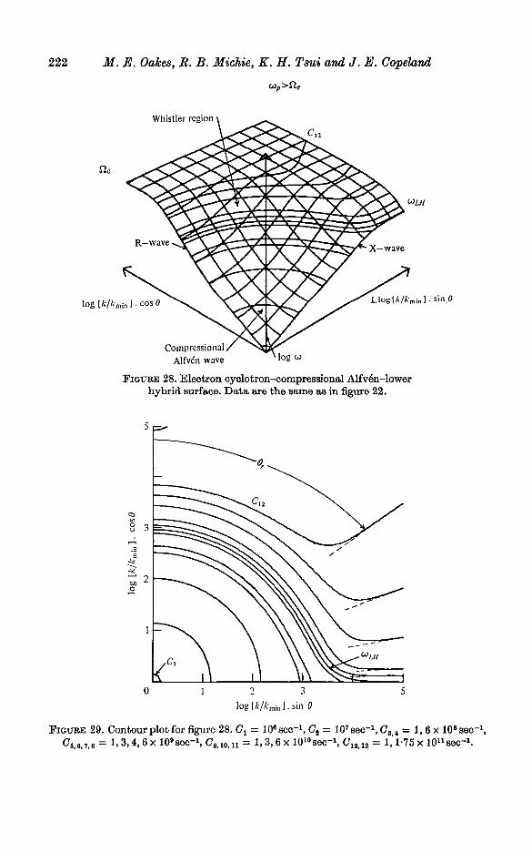
FIGUBE 28. Electron cyclotron-compressional Alfven-lowerhybrid surface. Data are the same as in figure 22.

FIGTJBB 29. Contour plot for figure 28. Gt = lO'sec-1, G2 = lO'sec"1, <73>4 = 1, 6 x 10s sec"1,£5,6,7.8= 1.3,4,6x10* sec-1, C 9 , 1 0 , u = l , 3 , 6 x lO^sec"1, C12,13 = 1,' 1-75 x 1011 sec-1.


log u

n,

log [k/km-m]. cos 0

log [k/kmin].sm9

Shear Alfven wave V "**" 'C,

FIOUBE 30. Shear Alfven-ion cyclotron surface. Data are the same as in figure 22.

5 i -

Jog [A-/Amin].sia0

FIGTJRE 31. Contour plot for figure 30. Contours C1>2tS = 1,3, 6 x 103sec-1>

^4,5,6 = 1.3,6 x 10'sec-1, (7, = 9-57 x'lb'sec"1.

surfaces and their contours. The discussion of the Unear plots applies to thesesurfaces.

Figure 22 shows five surfaces for a high density case (o)p > Q.e). We note inthis case that the compressional Alfv6n-lower hybrid surface now includes theelectron cyclotron wave. The upper hybrid surface now contains the plasmaoscillations along the magnetic field direction. The individual surfaces and their


contours are shown in figures 23-31. The labelling of the surfaces should besufficient explanation of the wave features.

Complete coverage of all cases included in the CMA diagram requires surfaceswith conditions such that o)pe < Cl{. The conditions for this case usually occuronly in the extremely thin low-density layer at the plasma surface; for this reasonthe surfaces are omitted from this paper. The inclusion of thermal modes willbe the subject of a future paper.

This work was supported by the Texas Atomic Energy Research Foundation.

REFERENCES

ALLIS, W. P. 1959 Sherwood Conference on Controlled Fusion, Oatlinburg, p. 32, TID-7682.ALLIS, W. P., BUCHSBAUM, S. J. & BEES, A. 1962 Waves in Plasmas. Wiley.

CLEMMOW, P. C. & MuiiLAiY, R. F. 1955 Physics of the Ionosphere, p. 340. PhysicalSociety, London.

STIX, T. H. 1962 The Theory of Plasma Waves. McGraw-Hill.STBINGEB, T. E. 1963 J. Nucl. Energy, Part 0, 5, 89.

cold plasma dispersion surfaces - repository home

Documents