cold start extra emissions as a function of engine stop time
TRANSCRIPT

ilable at ScienceDirect
Atmospheric Environment 43 (2009) 996–1007
Contents lists ava
Atmospheric Environment
journal homepage: www.elsevier .com/locate/atmosenv
Cold start extra emissions as a function of engine stop time: Evolutionover the last 10 years
Jean-Yves Favez*, Martin Weilenmann, Jan StilliEMPA, Laboratory for Internal Combustion Engines, Uberlandstrasse 129, 8600 Dubendorf, Zuerich, Switzerland
a r t i c l e i n f o
Article history:Received 6 September 2007Received in revised form 10 March 2008Accepted 14 March 2008
Keywords:Relative cold start extra (excess) emissionsStop (parking) timeLong-term evolutionExtra emission estimationGasoline passenger cars
* Corresponding author. Tel.: þ4144 823 4622; faE-mail address: [email protected] (J.-Y. Fa
1352-2310/$ – see front matter � 2008 Elsevier Ltddoi:10.1016/j.atmosenv.2008.03.037
a b s t r a c t
Cars with catalysts show a significant increase in exhaust emissions at engine start. Theseextra emissions are expressed as the difference, over a particular driving cycle, betweenemissions generated when the vehicle is started and when the engine or the catalyst arestably warm. Experimental data, suitable for the assessment of cold start emissions, areusually available for completely cooled engines. Most results originate from tests atambient temperature of 20–30 �C and with an engine stop time of at least 12 h. On theother hand, data including shorter stop times are very rare.The present work investigates the influence of exhaust emissions with shorter stop times,i.e. 0.5, 1, 2 and 4 h. The main goal consists in the comparison of emissions exhausted byrecent car models (Euro-4) against emissions assessed in the framework of a similarcampaign 10 years ago (FAV1/Euro-1 vehicles).A short survey of the current extra emission estimation methods is presented in this paper.It is shown that some methods are not suited for providing correct estimations in all cases.We discuss the fact that different estimation methods can show either similar orcompletely different results depending on the evolution behaviour of the hot emissions.Due to new technologies, e.g. the catalyst and improved engine control algorithms,emissions have been considerably reduced over the last 10 years. In this study it isdetermined how the relative extra emissions, i.e. extra emissions relative to the extraemissions for the standard stop time of 12 h, expressed as a function of stop time havechanged. We may claim with caution that for medium stop times of 0.5–4 h the averagerelative extra emissions of Euro-4 vehicles are well below the average of the relative extraemissions of Euro-1 vehicles.
� 2008 Elsevier Ltd. All rights reserved.
1. Introduction
Since catalysts are effective only at high temperature(the ‘light-off temperature’ which is above 200 �C), emis-sions are far more significant during the initial part (coldphase) of a trip when engine and catalyst are cold. Catalystshave become so effective in the last 15 years that it is evenbecoming difficult to measure the regulated pollutants, i.e.CO, HC and NOx, when the catalyst has reached its light-off
x: þ4144 823 4044.vez).
. All rights reserved.
temperature. Nowadays, due to catalyst improvements themost significant part of the total emission during a trip,especially for short trips (<10 km), takes place during thecold phase. Therefore, the analysis of additional emissionsduring the cold phase, referred to as the cold start extra (orexcess) emissions, has gradually gained significance inimproving emission models and thus emission inventories.
Cold start extra emissions can be subdivided into twoparts: (i) excess emissions due to the starting of the engineand (ii) excess emissions during the warming-up process ofthe engine and the catalyst. In this study only the sum isdiscussed. An exhaustive survey of research carried out inthe past concerning cold start emissions is given in the

Table 1Four gasoline vehicles which are considered for the Euro-1 campaign
Vehicle no. Make Model Eng. capacity (cc) Power (kW) Mileage (km) Gearbox type
1-1 BMW 325i 2493 125 133,264 Manual 52-1 BMW 320i 1989 95 154,662 Autom. 43-1 Opel Vectra GT 1997 85 65,912 Manual 54-1 VW Golf CL 1595 51 31,134 Manual 5
J.-Y. Favez et al. / Atmospheric Environment 43 (2009) 996–1007 997
report by Andre and Joumard (2005). We can sum up pastresearch by stating that it focuses on the characterisation ofcold start emissions as a function of the following fiveparameters: (i) technology or emission standard (FAV1/Euro-1 . Euro-4), (ii) average vehicle speed, 9 (iii) ambienttemperature, (iv) travelled distance and (v) engine stoptime (also called parking time). Large amounts of data andresearch results are available for the first four parameters,while suitable data for stop time analysis are very rare,since the measurement procedures required for suchinvestigations are time consuming and costly. Previous stoptime investigation results have been presented in Ham-marstrom (2002), Schweizer et al. (1997), Hausberger(1997) and Sabate (1996). In the present work we focus onstop times of 0, 0.5, 1, 2, 4 and 12 h by using 15 repetitiveIUFC (Inrets urbain fluide court, i.e. short free-flow urban)cycles (Andre et al., 1999).
This paper presents a brief survey of current extraemissions estimation methods. We show that somemethods are not suited for providing correct estimations inall cases. It is found that we have to distinguish betweendifferent hot phase emission classes, which have to beconsidered for the choice of the estimation method. Wediscuss the fact that different estimation methods can showeither similar or completely different results depending onthe hot phase emission class.
The main goal of this work is to describe the relative coldstart extra emissions as a function of stop times. We assumetherefore, as in Andre and Joumard (2005), that a stop timelonger than 12 h is sufficient to cool the engine and catalystdown to ambient temperature of 20–30 �C. Thus, the cycleafter a stop time of 12 h is considered as the fully cold-started cycle. The emissions of cycles with shorter stop timesare normalised by dividing by the emissions of the fullycold-started cycle. This results in a relative extra emission asa function of stop time. We present a comparison of relativeextra emissions in a recent campaign with Euro-4 gasolinepassenger vehicles against relative extra emissions assessedin the framework of a similar campaign 10 years ago withFAV1/Euro-1 gasoline passenger vehicles (Schweizer, 1997).Moreover, we compare the relative extra emissions of both
Table 2Six gasoline vehicles which are considered for the Euro-4 campaign
Vehicle no. Make Model Eng. capacity (cc
1-4 Opel Agila 1.2 11992-4 Fiat Stilo 1.6 15963-4 VW Sharan 1.8 17814-4 Toyota Avensis 2.0 19985-4 Ford Mondeo 2.5 24956-4 Audi A4 3.0 2976
campaigns with the INRETS model proposed by Andre andJoumard (2005).
2. Preliminaries
2.1. Experimental setup
The test fleet is composed of vehicles which reflect theSwiss fleet distribution with regard to engine size, chassistype and manufacturer of the single vehicle classes at thetime of selection. The cars are obtained from volunteerprivate owners and are not serviced before the test. All carswere tested on a chassis dynamometer test bench.Temperature and humidity are kept at reference valuesusing a closed-loop controller system. The exhaust gascomposition is determined in two different ways. Firstly,the gas is analysed in accordance with European CouncilDirective 70/220/EEC for passenger cars (Council Directive70/220/EEC, 1970), insofar as included. Under this proce-dure the exhaust gas has to be diluted with a constantvolume sampling (CVS) system and gas samples of thediluted exhaust and the ambient air are collected in bagsfor each section of the measured driving cycle. Secondly,undiluted (raw) online gas analysis measurements arecarried out at the tailpipe at 10 samples s�1. Thesemeasurements allow a more detailed analysis of thecorrelation between the driving pattern of the car andpollutant emissions and, for the purpose of this paper, arerequired for the subcycle analysis method.
The Euro-1 campaign was strictly speaking a FAV1campaign. But since the Swiss legislation FAV1 correspondsto the Euro-1 legislation we refer to as a Euro-1 campaign.The gasoline vehicles considered in this campaign are listedin Table 1. All four cars are equipped with a three-waycatalyst. The cycle considered is the T50 cycle which hasa length of 6.5 km, a duration of 830 s and an average speedof 28 km h�1. This cycle is a city-centre cycle which is notrepetitive, i.e. there is no identical driving pattern which isrepeated several times. The ambient temperature is set at25 �C and the ambient relative atmospheric humidityat 50%.
) Power (kW) Mileage (km) Gearbox type
55 46,492 Manual 576 77,801 Manual 5
110 101,065 Manual 6108 37,700 Autom. 4125 42,412 Manual 5162 49,938 ECVT

1 2 3 4 5 6 7 8 9 10 11 12 13 14 150
0.2
0.4
0.6
0.8
1
1.2
1.4
1.6
1.8
subcycle #
to
tal em
issio
ns p
er su
bcycle [g
/su
bcyc] cold start extra
emissions
hot phasecold phase
nc
Fig. 1. Evolution of emissions as a function of subcycle. Separation of the cycle into a cold and a hot phase.
1 2 3 4 5 6 7 8 9 10 11 12 13 14 15
0
–0.02
0.02
0.04
0.06
0.08
0.1
0.12
0.14
Subcycle #
Su
bcycle em
issio
n [g
/su
bcyc] Emission [g/subcycle]
Phase detection functionStart of hot emission part
nc
Fig. 2. Variations of the phase detection function as a function of subcycles.
J.-Y. Favez et al. / Atmospheric Environment 43 (2009) 996–1007998
Remarks: According to the report of Andre and Jou-mard (2005), the T50 cycle might be too short to captureall the cold phase emissions. This statement seems tocontradict results in the same report: for Euro-1 vehicleswith an ambient temperature of 25 �C and an averagespeed of 28 km h�1 cold distances (i.e. the distance of thecold phase) of 5.11 km for CO, 6.63 km for HC, 3.87 km forNOx and 6.1 km for CO2 are given. Thus, these suggestedcold distances are below the cycle length of 6.5 km,except for HC for which it is slightly above the cyclelength. These are, of course, averaged cold distances andsome cars could evidently show longer cold distances.But there is another fact that validates the use of T50cycles for cold start emission estimations. The results ofour Euro-4 campaign show that almost all cold distancesare about 1 km with an absolute cold distance maximumof 3 km (see Fig. 4, where the cold distances are aboutone IUFC cycle long). On the other hand, the averagedcold distances for Euro-4 vehicles suggested in Andre andJoumard (2005) are clearly above 1 km, i.e. with similarvalues as for the Euro-1 vehicles. This leads to theconclusion that the T50 cycle seems to be appropriate tocapture most of the cold phase emissions.
The characteristics of the gasoline Euro-4 test fleetvehicles are listed in Table 2. The cycle considered is theIUFC15 cycle, which is a repetition of 15 IUFC cycles (Andreet al., 1999). Only the first IUFC cycle includes the emissionsdue to the starting of the engine. There is no engine cut offduring the subsequent IUFC cycles. One IUFC cycle hasa length of 0.999 km, a duration of 189 s and an averagespeed of 19 km h�1. In what follows, the IUFC cycle isreferred to as the subcycle of the IUFC15 cycle. The ambienttemperature is set at 23 �C and the ambient relativeatmospheric humidity at 50%.
For each vehicle and stop time only one set of data, i.e.data of a unique driving cycle (IUFC15 or T50), is collected.
2.2. Cold start extra emissions estimation methods
For this work we consider following 4 cold start extraemissions estimation methods.
2.2.1. Subcycle analysis methodTo apply this method a repetitive cycle, such as the
IUFC15, is required. Fig. 1 illustrates this cycle as examplewith 15 subcycles. We have to separate the cycle intoa warm up phase, referred to as the cold phase, and a hotstabilised phase, referred to as the hot phase. Thus, we firsthave to determine which subcycles belong to the coldphase. In the case of Fig. 1 the seventh subcycle could beconsidered as the last subcycle of the cold phase, referred to

J.-Y. Favez et al. / Atmospheric Environment 43 (2009) 996–1007 999
as subcycle number nc. Following methods for determiningnc can be considered:
(a) It can be affected graphically ‘‘by hand’’ by analysing thetotal subcycle emissions as a function of the chrono-logically succeeding subcycles, which corresponds toa discretized time line.
(b) It can be computed by the standard deviation methoddeveloped at INRETS (see Andre and Joumard, 2005). Itconsists in computing the standard deviation backward,i.e. on the last two subcycles, then on the three lastsubcycles and then on all the following consecutivesubcycles. It is considered that during the hot phase theemissions are stable, except some small variations inthe emissions. In this case the standard deviationdecreases as a function of the increasing number ofsubcycles considered. However, as soon as cold startemissions appear the standard deviation increasesmore distinctly. Thus, at a certain subcycle a minimumstandard deviation emerge. This subcycle is defined asthe first hot subcycle, numbered as ncþ1, which leads tonc. During the present work it turned out that thismethod does not work in all cases. This is due to the fact
0 0. 5 1
0
–2
–4
–1
–0.5
2
4
CO
[g
/cyc]
Ford M
IUFCIUFC lin. reg.Int. BagComplete cycle
0 0.5 1
0
0.5
1
HC
[g
/cyc]
0 0.5 1
0
1
2
NO
x [g
/cyc]
0 0.5 1
0
200
400
CO
2 [g
/cyc]
stop
–200
Fig. 3. Extra emission as a function of stop time estimated b
that the cold start extra emissions are not emphasisedsufficiently after short stop times to permit accuratedetection. We therefore developed a more robustmethod to determine nc.
(c) This more robust method, referred to as the ‘‘enhancedstandard deviation method’’, requires the computationof the backward subcycle emission standard deviation(similar as for the INRETS standard deviation methoddescribed above) and the backward subcycle emissionaverage. The backward standard deviation is given bythe index function
sðnÞ ¼
ffiffiffiffiffiffiffiffiffiffiffiffiffiffiffiffiffiffiffiffiffiffiffiffiffiffiffiffiffiffiffiffiffiffiffiffiffiffiffiffiffiffiffiffiffiffiffiffiffiffiffiffiffiffiffi1
15� nP15
i¼nðEðiÞ � mðnÞÞ2r
if n ˛ f1;2;.;14g
0 if n ¼ 15
8<:
where
mðnÞ ¼ 116� n
X15
i¼n
EðiÞ;cn ˛ f1; 2;.;15g
is the index function of the backward average. The variablen represents the number of the subcycle. With both index
2 4 12
ondeo 2.5
2 4 12
2 4 12
2 4 12time [h]
y 4 different methods for vehicle 5-4 (Ford Mondeo).
J.-Y. Favez et al. / Atmospheric Environment 43 (2009) 996–10071000
functions and the emissions as a function of subcyclesa phase detection function is defined as follows:
f ðnÞ ¼�
EðnÞ � ðmðnÞ þ sðnÞÞ if n˛f1;2;.;15g0 if n ¼ 0
By means of this function nc is computed by determiningthe first subcycle, referred to as n0, for which f(n0)P0, whilethe subsequent subcycle, referred to as n0þ1, satisfiesf(n0þ1)<0. Mathematically, this can be expressed by a set
N ¼ fn ˛ f0;1;2;.;14g : f ðnÞP0 and f ðnþ 1Þ < 0g
and by nc¼min(n), cn ˛ NNote that for cycles for which no cold phase can be detected
nc is equal to 0. These are cycles for which the power train andthe catalyst are completely warmed-up from beginning.
Fig. 2 illustrates as an example the variations of the phasedetection function as a function of subcycles. For thisexample the set N has two elements N¼f2,9g. By taking thesmallest element of N, nc is equal to 2.
The idea behind this method is similar to that of the INRETSstandard deviation method. It is based on detecting increasedemissions (when f(n)>0) compared to the hot phase emis-sions, which is incorporated in f(n) by m(n), which refers tothe average of the hot phase emissions, and by s(n), whichrefers to the variations of the hot phase emissions. It has to be
0 0.5 10
1
2
3
4
CO
[g
/su
bcyc]
Ford Mo
0 0.5 10
0.5
1
HC
[g
/su
bcyc]
0 0.5 10
0.5
1
1.5
NO
x [g
/su
bcyc]
0 0.5 10
200
400
600
CO
2 [g
/su
bcyc]
stop t
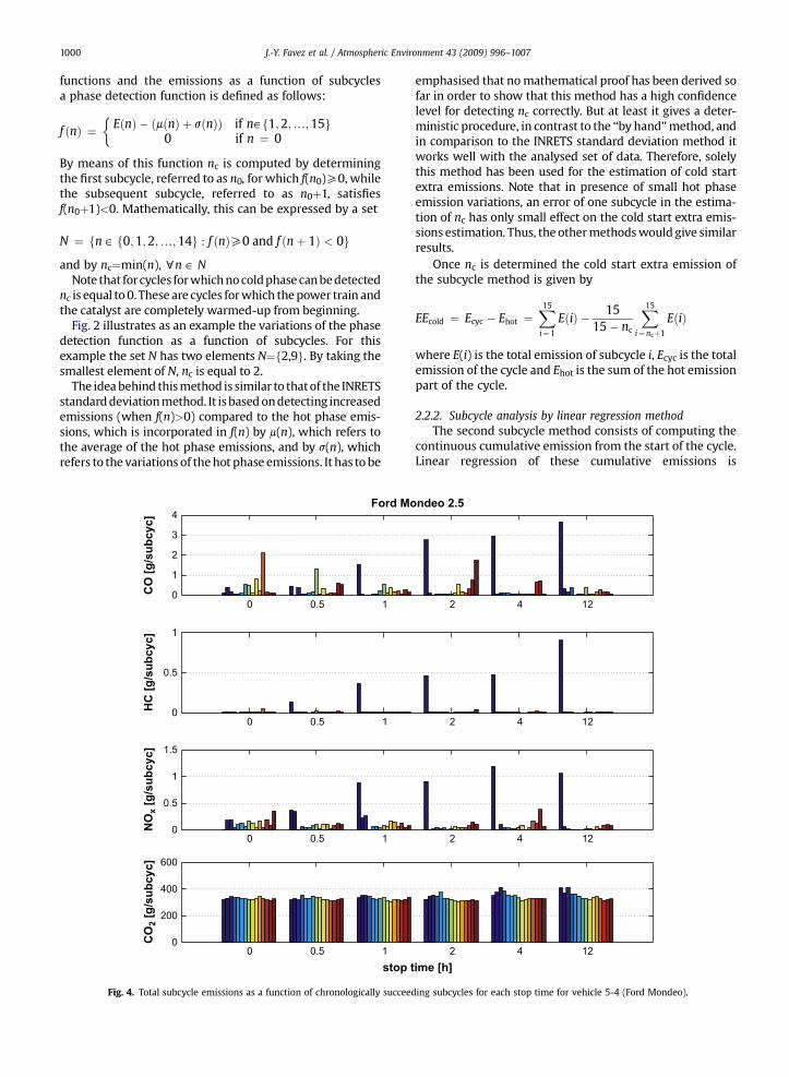
Fig. 4. Total subcycle emissions as a function of chronologically succee
emphasised that no mathematical proof has been derived sofar in order to show that this method has a high confidencelevel for detecting nc correctly. But at least it gives a deter-ministic procedure, in contrast to the ‘‘by hand’’ method, andin comparison to the INRETS standard deviation method itworks well with the analysed set of data. Therefore, solelythis method has been used for the estimation of cold startextra emissions. Note that in presence of small hot phaseemission variations, an error of one subcycle in the estima-tion of nc has only small effect on the cold start extra emis-sions estimation. Thus, the other methods would give similarresults.
Once nc is determined the cold start extra emission ofthe subcycle method is given by
EEcold ¼ Ecyc � Ehot ¼X15
i¼1
EðiÞ � 1515� nc
X15
i¼ncþ1
EðiÞ
where E(i) is the total emission of subcycle i, Ecyc is the totalemission of the cycle and Ehot is the sum of the hot emissionpart of the cycle.
2.2.2. Subcycle analysis by linear regression methodThe second subcycle method consists of computing the
continuous cumulative emission from the start of the cycle.Linear regression of these cumulative emissions is
2 4 12
ndeo 2.5
2 4 12
2 4 12
2 4 12ime [h]
ding subcycles for each stop time for vehicle 5-4 (Ford Mondeo).

J.-Y. Favez et al. / Atmospheric Environment 43 (2009) 996–1007 1001
calculated uniquely on the basis of the hot phase part. Thus,again nc is required and it is determined with the enhancedstandard deviation method presented above. Havingcomputed the linear regression as a function of subcycles,the estimation of the cold start extra emission is given byevaluating the linear regression at the first subcycle (startof the cycle). A detailed discussion of this method isprovided in Weilenmann (2001) and in Andre and Joumard(2005).
2.2.3. Bag analysis methodSome laboratories measure emission factors using bags
only. At EMPA a complete cycle is subdivided into three bagmeasurements. In the case of an IUFC15 the total emissionof subcycles 1–5, 6–10 and 11–15 correspond to the bags 1,2 and 3, respectively. By assuming that the cold phase endsbefore the start of the third bag (first 10 subcycles) theemission is given by
EEcold ¼ Ebag1 þ Ebag2 � 2Ebag3
2.2.4. Cycle analysis methodIf only the total emission of a whole cycle, referred to as
Ecyc, is available, we additionally need to measure the
0 0.5 1
0
−5
−50
5
10
CO
[g
/cyc]
Opel AIUFCIUFC lin. reg.Int. BagComplete cycle
0 0.5 10
0.5
1
1.5
HC
[g
/cyc]
0 0.5 10
0.2
0.4
0.6
0.8
NO
x [g
/cyc]
0 0.5 1
0
50
100
150
CO
2 [g
/cyc]
stop t
Fig. 5. Extra emission as a function of stop time estimated
emissions of a fully hot cycle, referred to as Ehotcyc. The coldstart extra emission is given by
EEcold ¼ Ecyc � Ehotcyc
A fully hot cycle starts with a completely warmed-uppower train and a catalyst above light-off temperature. Acycle after zero stop time can typically be considered asa fully hot cycle, if the engine start is not included in theconsidered cycle. Unfortunately, the engine start isincluded in the IUFC15 and the T50 cycles. For thesecycles the cold start extra emissions can be slightlyunderestimated due to the excess emissions during theengine start. Note that in the framework of this study noexcess emissions due to the engine start could beobserved.
This is the sole method which can be applied to non-repetitive cycles like the T50 cycle. But it can be as wellapplied to repetitive cycles like the IUFC15 cycle.
3. Comparison of the different extra emissionestimation methods
Fig. 3 illustrates the estimated cold start extra emissionsof vehicle 5–4 (Ford Mondeo). The extra emissions are
2 4 12
gila 1.2
2 4 12
2 4 12
2 4 12ime [h]
by 4 different methods for vehicle 1-4 (Opel Agila).

J.-Y. Favez et al. / Atmospheric Environment 43 (2009) 996–10071002
expressed as a function of stop time and are estimated withthe four different estimation methods by using data ofIUFC15 cycles. The extra emission of HC shows similarvalues for all methods, while for CO and NOx only thesubcycle methods provide similar extra emissions whichqualitatively correspond to the evolution that can beexpected. On the other hand, the bag and cycle methodsprovide widely varying and oscillating extra emissionevolutions.
These odd results can be explained by analysing theevolution of the subcycle emissions. Fig. 4 depicts thetotal subcycle emissions as a function of the chrono-logically succeeding subcycles for each stop time. Withthe focus only on the CO emissions, the first subcycle canbe assigned to the total cold start extra emissions. Thecycles corresponding to stop times of 0 and 2 h showa considerable excess of emissions in the last part oftheir hot phases, i.e. subcycles 10–15 (third bag), forwhich it is assumed that the catalyst light-off tempera-ture is already reached (especially for the 0 stop timecycle), and thus distinct lower emissions are expected.This emission excess therefore leads to negativeemission estimations for the bag analysis method. Asimilar observation can be established for the cycleanalysis method: Due to the excess emission during the
0 0.5 10
2
4
6
8
CO
[g
/su
bcyc]
Opel A
0 0.5 10
0.5
1
HC
[g
/su
bcyc]
0 0.5 10
0.4
0.2
0.6
0.8
NO
x [g
/su
bcyc]
0 0.5 10
100
200
300
CO
2 [g
/su
bcyc]
stop t
Fig. 6. Total subcycle emissions as a function of chronologically succe
last five subcycles of the zero stop time cycle (fully hotcycle) the hot phase emission Ehotcyc is overestimatedcompared to the hot phase emissions of the other cycles.This inevitably leads to an underestimation of the extraemissions particularly for the cycles corresponding tostop times of 2 and 4 h.
In general, it is expected to detect excess emissions forcycles with a stop time of 0 due to the starting of theengine. In our study this effect cannot be established. Atleast we claim that such an effect cannot be detected byinspecting the emissions as a function of subcycles(see Fig. 4).
Both subcycle analysis methods are in general morerobust, especially for cycles (such as the zero stop timecycle considered) for which no cold phase can be deter-mined, i.e. nc¼0. This robustness results from the fact thatthe hot phase emissions are averaged over several sub-cycles. In our considered case the cold phases end in sub-cycle one for stop time longer than 0 h, and thus the hotphase emissions are averaged over 14 subcycles, providingrepresentative hot phase emissions. We conclude that theestimation accuracy can be improved by increasing the hotphase length: either by appending supplementary sub-cycles or by measuring a cycle with the same stop timeseveral times.
2 4 12
gila 1.2
2 4 12
2 4 12
2 4 12ime [h]
eding subcycles for each stop time for vehicle 1-4 (Opel Agila).

0 0.5 1 2 4 120
5
10
15
CO
[g
/su
bcyc]
Toyota Avensis 2.0
0 0.5 1 2 4 120
3
2
1
HC
[g
/su
bcyc]
0 0.5 1 2 4 120
0.4
0.2
0.6
0.8
NO
x [g
/su
bcyc]
0 0.5 1 2 4 120
200
100
300
400
CO
2 [g
/su
bcyc]
stop time [h]
Fig. 7. Total subcycle emissions as a function of chronologically succeeding subcycles for each stop time for vehicle 4-4 (Toyota Avensis).
J.-Y. Favez et al. / Atmospheric Environment 43 (2009) 996–1007 1003
Similar considerations hold for the NOx emissions. Onthe other hand, the hot phase emissions of HC show lessvariation (Fig. 4). Thus, the subcycles in the hot phase (usedby the two subcycle methods), the third bag (used by thebag method) and the zero stop time cycle (used by the cyclemethod) have similar amounts of averaged emissions. Thisexplains the fact that the 4 methods provide similar extraemissions estimations for HC (Fig. 3).
By analysing the six vehicles of the recent Euro-4campaign we can distinguish between 3 different hot phaseclasses:
3.1. Homogeneous distributed hot phase emissions
For this class the hot phase emissions evolve almostconstantly with only small variations. Thus, all 4 extraemission estimation methods provide meaningful results.Fig. 5 illustrates the results for the different estimationmethods and Fig. 6 depicts the emissions as a function ofthe chronologically succeeding subcycles of vehicle 1–4(Opel Agila). Vehicles 3-4 and 6-4 show similar subcycleemissions and thus belong to this class regarding thepollutants CO, HC and NOx. In general, the HC pollutant forall vehicles also belongs to this class.
3.2. Heterogeneous distributed hot phase emissions
For this class the hot phase emissions oscillate and varygreatly. Thus, only the two subcycle analysis methods aresufficiently accurate. The CO and NOx pollutants of vehicles2-4 and 5-4 belong to this class. Fig. 3 illustrates the resultsfor the different estimation methods and Fig. 4 depicts theemissions as a function of the chronologically succeedingsubcycles of vehicle 5-4 (Ford Mondeo).
3.3. Non-determinable hot phase
The CO and NOx pollutants of vehicle 4-4 (ToyotaAvensis) show emission evolutions (Fig. 7) with thefollowing characteristics: (i) extreme subcycle emissionvariations, (ii) huge variations in averaged hot phaseemissions between cycles and (iii) for unusually many hotphase subcycles the emissions are larger than for coldphase subcycles.
Analysis of the air/fuel ratio of vehicle 4-4 reveals thatdifferent control strategies occur during the hot phases.Occasional air/fuel ratio drop peaks (Dl¼�0.15.�0.2) andincrease peaks (Dl¼þ0.01.þ0.03) lead to a considerableaugmentation of CO and NOx emissions respectively. It has

0 0.5 1 2 4 12
−50
−100
0
50
CO
[g
/cyc]
Toyota Avensis 2.0
0 0.5 1 2 4 12
0
1
2
3
HC
[g
/cyc]
0 0.5 1 2 4 12−2
−1
−1
0
1
2
0 0.5 1 2 4 12stop time [h]
IUFCIUFC lin. reg.Int. BagComplete cycle
−400
−200
0
200
400
NO
x [g
/cyc]
CO
2 [g
/cyc]
Fig. 8. Extra emission as a function of stop time estimated by 4 different methods for vehicle 4-4 (Toyota Avensis).
J.-Y. Favez et al. / Atmospheric Environment 43 (2009) 996–10071004
not yet been possible to establish the rule for these controlstrategies. Since the evolutions of the emissions showquasi-chaotic behaviour we conclude that for this type ofvehicles a meaningful estimation derived from anyproposed method cannot be expected. Fig. 8 illustrates the
0 2 4-1.5
-1
-0.5
0
0.5
1
1.5
2
2.5
extra em
issio
n [-]
stop t
CO of vehicle 4HC of vehicle 4
Fig. 9. Evolution of the normalised extra emission of the
results for the different estimation methods for vehicle 4-4(Toyota Avensis).
A possible explanation for hot phase emission variationscan be found by inspecting the mode of operation of thethree-way catalyst (TWC). The TWC requires the air/fuel
6 8 10 12
ime [h]
two Euro-1 samples excluded for the comparison.
CO
0 2 4 6 8 10 12-0.5
0
0.5
1
1.5
2
relative extra em
issio
n [-]
stop time [h]
Euro-4Euro-1Model
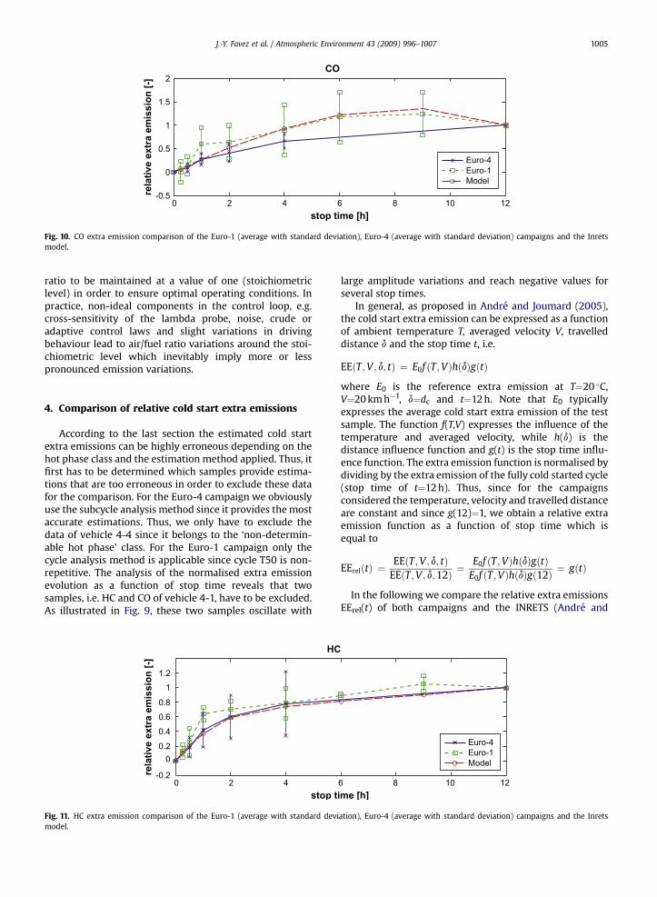
Fig. 10. CO extra emission comparison of the Euro-1 (average with standard deviation), Euro-4 (average with standard deviation) campaigns and the Inretsmodel.
J.-Y. Favez et al. / Atmospheric Environment 43 (2009) 996–1007 1005
ratio to be maintained at a value of one (stoichiometriclevel) in order to ensure optimal operating conditions. Inpractice, non-ideal components in the control loop, e.g.cross-sensitivity of the lambda probe, noise, crude oradaptive control laws and slight variations in drivingbehaviour lead to air/fuel ratio variations around the stoi-chiometric level which inevitably imply more or lesspronounced emission variations.
4. Comparison of relative cold start extra emissions
According to the last section the estimated cold startextra emissions can be highly erroneous depending on thehot phase class and the estimation method applied. Thus, itfirst has to be determined which samples provide estima-tions that are too erroneous in order to exclude these datafor the comparison. For the Euro-4 campaign we obviouslyuse the subcycle analysis method since it provides the mostaccurate estimations. Thus, we only have to exclude thedata of vehicle 4-4 since it belongs to the ‘non-determin-able hot phase’ class. For the Euro-1 campaign only thecycle analysis method is applicable since cycle T50 is non-repetitive. The analysis of the normalised extra emissionevolution as a function of stop time reveals that twosamples, i.e. HC and CO of vehicle 4-1, have to be excluded.As illustrated in Fig. 9, these two samples oscillate with
HC
0 2 4-0.2
00.2
0.4
0.6
0.8
11.2
relative extra em
issio
n [-]
stop t
Fig. 11. HC extra emission comparison of the Euro-1 (average with standard devimodel.
large amplitude variations and reach negative values forseveral stop times.
In general, as proposed in Andre and Joumard (2005),the cold start extra emission can be expressed as a functionof ambient temperature T, averaged velocity V, travelleddistance d and the stop time t, i.e.
EEðT;V ; d; tÞ ¼ E0f ðT;VÞhðdÞgðtÞ
where E0 is the reference extra emission at T¼20 �C,V¼20 km h�1, d¼dc and t¼12 h. Note that E0 typicallyexpresses the average cold start extra emission of the testsample. The function f(T,V) expresses the influence of thetemperature and averaged velocity, while h(d) is thedistance influence function and g(t) is the stop time influ-ence function. The extra emission function is normalised bydividing by the extra emission of the fully cold started cycle(stop time of t¼12 h). Thus, since for the campaignsconsidered the temperature, velocity and travelled distanceare constant and since g(12)¼1, we obtain a relative extraemission function as a function of stop time which isequal to
EErelðtÞ ¼EEðT ;V ; d; tÞ
EEðT;V ; d;12Þ ¼E0f ðT ;VÞhðdÞgðtÞ
E0f ðT;VÞhðdÞgð12Þ ¼ gðtÞ
In the following we compare the relative extra emissionsEErel(t) of both campaigns and the INRETS (Andre and
6 8 10 12ime [h]
Euro-4Euro-1Model
ation), Euro-4 (average with standard deviation) campaigns and the Inrets

NOx
0 2 4 6 8 10 12-0.5
0
0.5
1
1.5
2
2.5
3
relative extra em
issio
n [-]
Euro-4Euro-1Model
stop time [h]
Fig. 12. NOx extra emission comparison of the Euro-1 (average with standard deviation), Euro-4 (average with standard deviation) campaigns and the Inretsmodel.
J.-Y. Favez et al. / Atmospheric Environment 43 (2009) 996–10071006
Joumard, 2005) model against each other. Note that theINRETS model consists of polynomials as a function of stoptime.
CO (Fig. 10): The standard deviations indicate that theCO mean variations of Euro-1 vehicles are much larger asfor Euro-4 vehicles. The model fits the Euro-1 data well,except at t¼1 h. This result is not surprising since the modelis based on older vehicle data. For stop times longer than1 h the relative extra emissions of the Euro-4 vehicles arewell below the modelled and averaged Euro-1 extraemissions.
HC (Fig. 11): In contrast to CO, the HC mean variationsare much larger for the Euro-4 vehicles. Surprisingly, themodel fits the Euro-4 vehicles much better than the Euro-1vehicles. The HC relative extra emissions of the Euro-4vehicles are appreciably below the Euro-1 emissions in thestop time interval of 0.5–4 h.
NOx (Fig. 12): In the stop time interval of 0.5–4 h theEuro-4 campaign fleet produce lower NOx relative extraemissions than the Euro-1 fleet. But as the standard devi-ations are large for both campaigns this establishmentshould be viewed with caution. By taking into consider-ation the large standard deviations the model can beregarded as appropriate for representing both Euro-1 andEuro-4 vehicles.
Note that there is a similar tendency for CO, HC and NOx
that the Euro-1 campaign show higher relative cold startextra emissions than the model at stop times 1 and 2 h.
CO2: With regard to the Euro-4 vehicles, potential rela-tive extra emissions can only be detected for 12 h stop timecycles. Thus, no particular statements concerning therelative extra emissions for the relevant stop times (#4 h)can be deduced, apart the fact that they seem to beapproximately zero. Similarly, no trends can be detected forthe Euro-1 test fleet. This is remarkable, since other reports,e.g. Hammarstrom (2002) and Andre and Joumard (2005),claim to identify clear trends as a function of stop time forEuro-1 cars. The following two causes could explain thisdifference. Firstly, in this study only the cycle method couldbe applied for the Euro-1 test fleet. As mentioned above thecycle method is not as accurate as the subcycle methods.Secondly, we cannot average out several data sets sinceonly one set of data per vehicle and stop time is available.Therefore, it is not possible to remove random emission
variations in order to potentially establish stressed trends.Further investigations are required in order to identify thepredominant factor for this discrepancy.
5. Discussion and conclusion
The comparison of the different extra emission esti-mation methods clearly indicates that the bag and cyclemethods often fail when the hot phase emissions varygreatly. Thus, in general, one of the two distinctly morerobust subcycle methods should be preferably applied inorder to ensure meaningful estimation results. Neverthe-less, there are vehicles for which the extra emissionscannot be estimated with any proposed methods. In suchcases an improvement can probably only be achieved byconsiderably increasing the number of tests in order toobtain more accurate averaged hot phase emission esti-mations. Since the estimation methods may fail it isimportant to examine the resulting estimations in order toexclude non-meaningful data for interpretation andmodelling purposes.
Currently we are not in the position to explain the wideemission variations during the hot phase. Therefore, weconsider that the next steps should be the determinationand characterisation of the causes of this phenomenon.Further analysis of emission variations during the hotphase are most important, especially if there are systematicchanges as a function of time and distance when theidentical cycle is repeated.
For the relative extra emission comparison it is difficultto state trends with great certainty since only a few vehiclesare considered, i.e. three vehicles for Euro-1 and five forEuro-4. Nevertheless, we may claim with caution that formedium stop times of 0.5 to 4 h the averaged relative coldstart extra emissions of recent vehicles (Euro-4) are wellbelow the averaged extra emissions of 10-year-old vehicles.This new result may prove useful for expanding the INRETSand other models with stop time influences of Euro-4vehicles.
In this paper we mentioned that the estimated colddistance of the six examined Euro-4 vehicles are about1 km, while in Andre and Joumard (2005) the colddistances evaluated from data of 14 gasoline Euro-4 vehi-cles are given as follows: 5.2 km for CO, 6.6 km for HC,

J.-Y. Favez et al. / Atmospheric Environment 43 (2009) 996–1007 1007
3.9 km for NOx and 1.9 km for CO2. Thus, this large discrep-ancy has to be investigated in order to be able to providea consistent model.
Acknowledgements
This work was done within the DACHþNLþS (German,Austrian, Swiss, Dutch and Swedish) cooperation on vehicleemission monitoring. The authors wish to thank FOEN,FEDRO, SFOE and all co-founders.
References
Andre, J-M., Joumard, R., 2005. Modelling of cold start excess emissionsfor passenger cars. INRETS Report, No. LTE 0509, Bron, France, 239pp.
Andre, M., Hammarstrom, U., Reynaud, I., 1999. Driving Statistics for theassessment of pollutant emissions from road transport. INRETSReport, No. LTE9906, Bron, France.
Council Directive 70/220/EEC 1970. On the approximation of the lawsof the Member States relating to measures to be taken against
air pollution by gases from positive-ignition engines of motor vehi-cles Chttp://eur-lex.europa.eu/LexUriServ/LexUriServ.do?uri¼CELEX:31970L0220:EN:NOTD.
Hammarstrom, U., 2002. Betydelsen av korta motoravstangningar ochkortid for avgasemissioner fran bensindrivna bilar med och utankatalysator (Exhaust emission variations for short engine stops anddriving time for petrol cars with and without catalyst). VTI medde-lande 931, Sweden.
Hausberger, S., 1997. Globale Modellbildung fur Emissions- und Ver-brauchsszenarien im Verkehrssektor (Global modelling of scenariosconcerning emission and fuel consumption in the transport sector).Dissertation am Institut fur Verbrennungskraftmaschinen und Ther-modynamik der TU-Graz, Graz.
Sabate, S., 1996. Methodology for calculating and redefining cold and hotstart emissions. CARB Report.
Schweizer, Th., Rytz, Ch., Heeb, N., Mattrel, P., 1997. Nachfuhrung derEmissionsgrundlagen Strassenverkehr–Teilprojekt Emissionsfakto-ren–Arbeiten 1996 (Tracing of emission bases-road traffic–subproject emission factors–work in 1996). EMPA Bericht-Nr.161’150.
Weilenmann, M.F., 2001. Cold start and cold ambient emissions of Euro IIcars. In: Proceedings of the 10th International Symposium on Trans-port and Air Pollution, Boulder, USA.