ÉCOLE DE TECHNOLOGIE SUPÉRIEUREUNIVERSITÉ DU QUÉBEC

THESIS PRESENTED TOÉCOLE DE TECHNOLOGIE SUPÉRIEURE

IN PARTIAL FULFILLMENT OF THE REQUIREMENTS FORTHE DEGREE OF DOCTOR OF PHILOSOPHY

Ph.D.

BYLuana BEZERRA BATISTA

MULTI-CLASSIFIER SYSTEMS FOR OFF-LINE SIGNATURE VERIFICATION

MONTREAL, MARCH 30 2011

c© Copyright 2011 reserved by Luana Bezerra Batista

BOARD OF EXAMINERS

THIS THESIS HAS BEEN EVALUATED

BY THE FOLLOWING BOARD OF EXAMINERS

Mr. Robert Sabourin, thesis directorDépartement de génie de la production automatisée à l’École de technologie supérieure

Mr. Eric Granger, thesis co-directorDépartement de génie de la production automatisée à l’École de technologie supérieure

Mr. Bruno De Kelper, committee presidentDépartement de génie électrique à l’École de technologie supérieure

Mr. Jean-Marc Robert, examinerDépartement de génie logiciel et des technologies de l’information

Mrs. Nicole Vincent, external examinerUniversité Paris Descartes

THIS THESIS HAS BEEN PRESENTED AND DEFENDED

BEFORE A BOARD OF EXAMINERS AND PUBLIC

MARCH 14 2011

AT ÉCOLE DE TECHNOLOGIE SUPÉRIEURE

ACKNOWLEDGMENTS

First of all, I would like to thank Dr. Robert Sabourin and Dr. Eric Granger, for supervi-

sing my work over these five years. Their expertise and guidance were fundamental for the

accomplishment of this Thesis.

Thanks also to the members of my examining committee: Dr. Nicole Vincent, Dr. Jean-Marc

Robert and Dr. Bruno De Kelper, for evaluating this Thesis and providing valuable comments.

I would like to thank all my colleagues in the LIVIA (Laboratoire d’imagerie, de vision et

d’intelligence artificielle), for sharing so many ideas, and Vins et Fromages. Special thanks to

Albert Ko, Bassem Guendy, Carlos Cadena, Clement Chion, César Alba, Cristophe Pagano,

David Dubois, Dominique Rivard, Eduardo Vellasques, Éric Thibodeau, Eulanda dos San-

tos, Francis Quintal, George Eskander, Idrissa Coulibaly, Jean-François Connoly, Jonathan

Bouchard, Jonathan Milgram, Luis da Costa, Marcelo Kapp, Mathias Adankon, Melyssa Ay-

ala, Miguel de la Torre, Olaf Gagnon, Paulo Cavalin, Vincent Doré, and Wael Khreich.

Most of all, thanks to my boyfriend, Julien Lauzé, as well as to Ana Aguiar, Fernando Kajita,

Jean-Pierre Caradant, Larissa Fernandes, Linda Henrichon, and Paulino Neto, for being my

new family in Montreal.

I dedicate this Thesis to all my friends and family in Brazil, especially to my mother, Ligia

Bezerra, my sister, Beatriz Bezerra, my aunt, Nina Bezerra, and my grandmother, Inah Bezerra.

They have always supported and encouraged me.

This work was financially supported by the Defence Research and Development Canada, by

the Fonds Québécois de la Recherche sur la Nature et les Technologies, and by the Natural

Sciences and Engineering Research Council of Canada.

MULTI-CLASSIFIER SYSTEMS FOR OFF-LINE SIGNATURE VERIFICATION

Luana BEZERRA BATISTA

ABSTRACT

Handwritten signatures are behavioural biometric traits that are known to incorporate a con-siderable amount of intra-class variability. The Hidden Markov Model (HMM) has been suc-cessfully employed in many off-line signature verification (SV) systems due to the sequentialnature and variable size of the signature data. In particular, the left-to-right topology of HMMsis well adapted to the dynamic characteristics of occidental handwriting, in which the handmovements are always from left to right. As with most generative classifiers, HMMs requirea considerable amount of training data to achieve a high level of generalization performance.Unfortunately, the number of signature samples available to train an off-line SV system is verylimited in practice. Moreover, only random forgeries are employed to train the system, whichmust in turn to discriminate between genuine samples and random, simple and skilled forgeriesduring operations. These last two forgery types are not available during the training phase.

The approaches proposed in this Thesis employ the concept of multi-classifier systems (MCS)based on HMMs to learn signatures at several levels of perception. By extracting a high numberof features, a pool of diversified classifiers can be generated using random subspaces, whichovercomes the problem of having a limited amount of training data.

Based on the multi-hypotheses principle, a new approach for combining classifiers in the ROCspace is proposed. A technique to repair concavities in ROC curves allows for overcomingthe problem of having a limited amount of genuine samples, and, especially, for evaluatingperformance of biometric systems more accurately. A second important contribution is theproposal of a hybrid generative-discriminative classification architecture. The use of HMMsas feature extractors in the generative stage followed by Support Vector Machines (SVMs) asclassifiers in the discriminative stage allows for a better design not only of the genuine class,but also of the impostor class. Moreover, this approach provides a more robust learning thana traditional HMM-based approach when a limited amount of training data is available. Thelast contribution of this Thesis is the proposal of two new strategies for the dynamic selection(DS) of ensemble of classifiers. Experiments performed with the PUCPR and GPDS signaturedatabases indicate that the proposed DS strategies achieve a higher level of performance inoff-line SV than other reference DS and static selection (SS) strategies from literature.

Keywords : Dynamic Selection, Ensembles of Classifiers, Hidden Markov Models, HybridGenerative-Discriminative Systems, Multi-Classifier Systems, Off-line Signature Verification,ROC Curves, Support Vector Machines.

SYSTÈMES DE CLASSIFICATEURS MULTIPLES POUR LA VÉRIFICATIONHORS-LIGNE DE SIGNATURES MANUSCRITES

Luana BEZERRA BATISTA

RÉSUMÉ

Les signatures manuscrites sont des traits biométriques comportementaux caractérisés par unegrande variabilité intra-classe. Les modèles de Markov cachés (MMCs) ont été utilisés avecsuccès en vérification hors-ligne des signatures manuscrites (VHS) en raison de la nature sé-quentielle et très variable de la signature. En particulier, la topologie gauche-droite des MMCsest très bien adaptée aux caractéristiques de l’écriture occidentale, dont les mouvements de lamain sont principalement exécutés de la gauche vers la droite. Comme la plupart des classifi-cateurs de type génératif, les MMCs requièrent une quantité importante de données d’entraî-nement pour atteindre un niveau de performance élevé en généralisation. Malheureusement, lenombre de signatures disponibles pour l’apprentissage des VHS est très limité en pratique. Deplus, uniquement les faux aléatoires sont utilisés pour l’apprentissage des VHS qui doivent êtreen mesure de discriminer entre les signatures authentiques et les classes de faux aléatoires, lesfaux simples et les imitations. Ces deux dernières classes de faux ne sont pas disponibles lorsde la phase d’apprentissage.

Les approches proposées dans cette thèse reposent sur le concept des classificateurs multiplesbasés sur des MMCs exploités pour l’extraction de plusieurs niveaux de perception des signa-tures. Cette stratégie basée sur la génération d’un nombre très important de caractéristiquespermet la mise en œuvre de classificateurs dans les sous-espaces aléatoires, ce qui permet des’affranchir du nombre limité de données disponibles pour l’entraînement.

Une nouvelle approche pour la combinaison des classificateurs basée sur le principe des hy-pothèses multiples dans l’espace ROC est proposée. Une technique de réparation des courbesROC permet de s’affranchir du nombre limité de signatures disponibles et surtout pour l’éva-luation de la performance des systèmes biométriques. Une deuxième contribution importanteest la proposition d’une architecture de classification hybride de type génératif-discriminatif.L’utilisation conjointe des MMCs pour l’extraction des caractéristiques et des machines à vec-teurs de support (MVSs) pour la classification permet une meilleure représentation non seule-ment de la classe des signatures authentiques, mais aussi de la classe des imposteurs. L’ap-proche proposée permet un apprentissage plus robuste que les approches MMCs convention-nelles lorsque le nombre d’échantillons disponibles est limité. La dernière contribution de cettethèse est la proposition de deux nouvelles stratégies pour la sélection dynamique (SD) d’en-sembles de classificateurs. Les résultats obtenus sur les bases de signatures manuscrites PUCPRet GPDS, montrent que les stratégies proposées sont plus performantes que celles publiées dansla littérature pour la sélection dynamique ou statique des ensembles de classificateurs.

VI

Mots-clés : Courbes ROC, ensembles de classificateurs, machines à vecteurs de support, mo-dèles de Markov cachés, sélection dynamique de classificateurs, systèmes hybrides génératifs-discriminatifs, systèmes à classificateurs multiples, vérification hors-ligne des signatures ma-nuscrites.

TABLE OF CONTENT

Page

INTRODUCTION................................................................................................ 1

CHAPTER 1 THE STATE-OF-THE-ART IN OFF-LINE SIGNATURE VERIFICATION 101.1 Feature Extraction Techniques ................................................................... 11

1.1.1 Signature Representations ............................................................. 121.1.2 Geometrical Features.................................................................... 151.1.3 Statistical Features....................................................................... 171.1.4 Similarity Features....................................................................... 181.1.5 Fixed Zoning .............................................................................. 181.1.6 Signal Dependent Zoning .............................................................. 201.1.7 Pseudo-dynamic Features .............................................................. 23

1.2 Verification Strategies and Experimental Results............................................ 251.2.1 Performance Evaluation Measures................................................... 251.2.2 Distance Classifiers...................................................................... 261.2.3 Artificial Neural Networks............................................................. 281.2.4 Hidden Markov Models ................................................................ 291.2.5 Dynamic Time Warping ................................................................ 311.2.6 Support Vector Machines .............................................................. 321.2.7 Multi-Classifier Systems ............................................................... 33

1.3 Dealing with a limited amount of data ......................................................... 351.4 Discussion............................................................................................. 38

CHAPTER 2 A MULTI-HYPOTHESIS APPROACH.............................................. 422.1 Off-line SV systems based on discrete HMMs............................................... 44

2.1.1 Feature Extraction ....................................................................... 452.1.2 Vector Quantization ..................................................................... 472.1.3 Classification.............................................................................. 47

2.2 Challenges with the Single-Hypothesis Approach .......................................... 492.3 The Multi-Hypothesis Approach ................................................................ 53

2.3.1 Model Selection .......................................................................... 542.3.2 Combination .............................................................................. 562.3.3 Averaging .................................................................................. 562.3.4 Testing ...................................................................................... 57

2.4 Experimental Methodology ....................................................................... 582.5 Simulation Results and Discussions ............................................................ 62

2.5.1 Off-line SV based on an universal codebook...................................... 622.5.2 Off-line SV based on user-specific codebooks.................................... 69

2.6 Discussion............................................................................................. 73

VIII

CHAPTER 3 DYNAMIC SELECTION OF GENERATIVE-DISCRIMINATIVEENSEMBLES................................................................................ 76

3.1 Hybrid Generative-Discriminative Ensembles ............................................... 773.2 A System for Dynamic Selection of Generative-Discriminative Ensembles.......... 80

3.2.1 System Overview ........................................................................ 803.2.2 Bank of HMMs........................................................................... 843.2.3 A Random Subspace Method for Two-Class Classifiers ....................... 853.2.4 A New Strategy for Dynamic Ensemble Selection .............................. 873.2.5 Complexity Analysis .................................................................... 91

3.3 Experimental Methodology ....................................................................... 923.3.1 Off-line SV Databases .................................................................. 92

3.3.1.1 Brazilian SV database ....................................................... 933.3.1.2 GPDS database................................................................ 93

3.3.2 Grid Segmentation....................................................................... 953.3.3 Training of the Generative Stage .................................................... 963.3.4 Training of the Discriminative Stage................................................ 973.3.5 Classifier Ensemble Selection......................................................... 983.3.6 Performance Evaluation ................................................................ 99

3.4 Simulation Results and Discussions ........................................................... 1003.4.1 Reference Systems...................................................................... 1003.4.2 Scenario 1 – abundant data ........................................................... 1013.4.3 Scenario 2 – sparse data ............................................................... 1033.4.4 Comparisons with systems in the literature....................................... 1083.4.5 System Complexity..................................................................... 110

3.5 Discussion............................................................................................ 111

CONCLUSION ................................................................................................ 113

APPENDIX I STATIC SELECTION OF GENERATIVE-DISCRIMINATIVE EN-SEMBLES ................................................................................... 118

APPENDIX II ADDITIONAL RESULTS OBTAINED WITH THE HYBRIDGENERATIVE-DISCRIMINATIVE SYSTEM .................................... 125

APPENDIX III USING SYSTEM-ADAPTED CODEBOOKS ................................. 131

LIST OF TABLES

Page

Table 1.1 Signature verification databases (I = Individual; G = Genuine; F =Forgeries; S = Samples) . . . . . . . . . . . . . . . . . . . . . . . . . . . . . . . . . . . . . . . . . . . . . . . . . . . . . . . . . 41

Table 2.1 Error rates (%) on test . . . . . . . . . . . . . . . . . . . . . . . . . . . . . . . . . . . . . . . . . . . . . . . . . . . . . . . . . . . 68

Table 2.2 Additional error rates (%) on test obtained with the multi-hypothesis system 68

Table 2.3 Error rates (%) on test . . . . . . . . . . . . . . . . . . . . . . . . . . . . . . . . . . . . . . . . . . . . . . . . . . . . . . . . . . . 71

Table 3.1 Time complexities of the generative and discriminative stages . . . . . . . . . . . . . . . . 91

Table 3.2 Datasets for a specific writer i, using the Brazilian SV database . . . . . . . . . . . . . . 94

Table 3.3 Datasets for a specific writer i, using the GPDS database . . . . . . . . . . . . . . . . . . . . . 95

Table 3.4 Overall error rates (%) obtained on Brazilian test data for γ = 0.90,under Scenario 1 . . . . . . . . . . . . . . . . . . . . . . . . . . . . . . . . . . . . . . . . . . . . . . . . . . . . . . . . . . . . . . . .103

Table 3.5 Overall error rates (%) obtained on Brazilian test data for γ = 1.0,under Scenario 1 . . . . . . . . . . . . . . . . . . . . . . . . . . . . . . . . . . . . . . . . . . . . . . . . . . . . . . . . . . . . . . . .103

Table 3.6 Overall error rates (%) obtained on Brazilian and GPDS-160 testdata for γ = 0.90, under Scenario 2. . . . . . . . . . . . . . . . . . . . . . . . . . . . . . . . . . . . . . . . . . . .107

Table 3.7 Overall error rates (%) provided by systems designed with theBrazilian SV database . . . . . . . . . . . . . . . . . . . . . . . . . . . . . . . . . . . . . . . . . . . . . . . . . . . . . . . . . .109

Table 3.8 EERs (%) provided by the proposed system and by other systemsin the literature . . . . . . . . . . . . . . . . . . . . . . . . . . . . . . . . . . . . . . . . . . . . . . . . . . . . . . . . . . . . . . . . . .110

Table 3.9 Average number of HMMs, states, SVM inputs, and support vectors(SVs) in each scenario . . . . . . . . . . . . . . . . . . . . . . . . . . . . . . . . . . . . . . . . . . . . . . . . . . . . . . . . . .111

LIST OF FIGURES

Page

Figure 0.1 Examples of (a) genuine signature, (b) random forgery, (c) simpleforgery and (d) skilled forgery. . . . . . . . . . . . . . . . . . . . . . . . . . . . . . . . . . . . . . . . . . . . . . . . . . . 2

Figure 0.2 Block diagram of a generic SV system. . . . . . . . . . . . . . . . . . . . . . . . . . . . . . . . . . . . . . . . . 3

Figure 0.3 Example of several superimposed signature samples of the same writer. . . . . . 4

Figure 1.1 Examples of (a) Occidental and (b) Japanese signatures.Adapted from Justino (2001) . . . . . . . . . . . . . . . . . . . . . . . . . . . . . . . . . . . . . . . . . . . . . . . . . . . 10

Figure 1.2 Examples of (a) (b) cursive and (c) graphical signatures. . . . . . . . . . . . . . . . . . . . . . 11

Figure 1.3 A taxonomy of feature types used in SV. . . . . . . . . . . . . . . . . . . . . . . . . . . . . . . . . . . . . . . 12

Figure 1.4 Examples of (a) handwritten signature and (b) its outline.Adapted from Huang and Yan (1997). . . . . . . . . . . . . . . . . . . . . . . . . . . . . . . . . . . . . . . . . . 13

Figure 1.5 Signature outline extraction using morphological operations: (a)original signature, (b) dilated signature, (c) filled signature and (d)signature outline.Adapted from Ferrer et al. (2005) . . . . . . . . . . . . . . . . . . . . . . . . . . . . . . . . . . . . . . . . . . . . . . 14

Figure 1.6 Examples of (a) handwritten signature and (b) its upper and lowerenvelopes.Adapted from Bertolini et al. (2010) . . . . . . . . . . . . . . . . . . . . . . . . . . . . . . . . . . . . . . . . . . . 14

Figure 1.7 Examples of signatures with two different calibers: (a) large, and(b) medium.Adapted from Oliveira et al. (2005). . . . . . . . . . . . . . . . . . . . . . . . . . . . . . . . . . . . . . . . . . . . 15

Figure 1.8 Examples of (a) proportional, (b) disproportionate, and (c) mixedsignatures.Adapted from Oliveira et al. (2005). . . . . . . . . . . . . . . . . . . . . . . . . . . . . . . . . . . . . . . . . . . . 16

Figure 1.9 Examples of signatures (a) with spaces and (b) no space.Adapted from Oliveira et al. (2005). . . . . . . . . . . . . . . . . . . . . . . . . . . . . . . . . . . . . . . . . . . . 16

Figure 1.10 Examples of signatures with an alignment to baseline of (a) 22◦,and (b) 0◦.Adapted from Oliveira et al. (2005). . . . . . . . . . . . . . . . . . . . . . . . . . . . . . . . . . . . . . . . . . . . 17

XI

Figure 1.11 Grid segmentation using (a) square cells and (b) rectangular cells.Adapted from Justino et al. (2000) . . . . . . . . . . . . . . . . . . . . . . . . . . . . . . . . . . . . . . . . . . . . . 19

Figure 1.12 Examples of (a) handwritten signature and (b) its envelopes.Adapted from Bajaj and Chaudhury (1997) . . . . . . . . . . . . . . . . . . . . . . . . . . . . . . . . . . . 21

Figure 1.13 Retina used to extract local Granulometric Size Distributions.Adapted from Sabourin et al. (1997b) . . . . . . . . . . . . . . . . . . . . . . . . . . . . . . . . . . . . . . . . . 21

Figure 1.14 Example of feature extraction on a looping stroke by the ExtendedShadow Code technique. Pixel projections on the bars are shownin black.Adapted from Sabourin et al. (1993). . . . . . . . . . . . . . . . . . . . . . . . . . . . . . . . . . . . . . . . . . . 22

Figure 1.15 Example of polar sampling on an handwritten signature. Thecoordinate system is centered on the centroid of the signature toachieve translation invariance and the signature is sampled using asampling length α and an angular step β.Adapted from Sabourin et al. (1997a) . . . . . . . . . . . . . . . . . . . . . . . . . . . . . . . . . . . . . . . . . 22

Figure 1.16 Examples of (a) signature and (b) its high pressure regions.Adapted from Huang and Yan (1997). . . . . . . . . . . . . . . . . . . . . . . . . . . . . . . . . . . . . . . . . . 24

Figure 1.17 Examples of stroke progression: (a) few changes in directionindicates a tense stroke, and (b) a limp stroke changes directionmany times.Adapted from Oliveira et al. (2005). . . . . . . . . . . . . . . . . . . . . . . . . . . . . . . . . . . . . . . . . . . . 24

Figure 1.18 Additional Sample Generation: (a) Pair of genuine samplesoverlapped, (b) The corresponding strokes identified and linkedup by displacement vectors, (c) New sample generated byinterpolation (dashed lines with dots).Adapted from Fang and Tang (2005) . . . . . . . . . . . . . . . . . . . . . . . . . . . . . . . . . . . . . . . . . . 37

Figure 1.19 Examples of computer generated signatures (in grey), obtainedusing an strategy based on elastic matching, and the originalsignatures (in black).Adapted from Fang and Tang (2005) . . . . . . . . . . . . . . . . . . . . . . . . . . . . . . . . . . . . . . . . . . 37

Figure 2.1 Block diagram of a traditional off-line SV system based on discrete HMMs.45

Figure 2.2 Example of grid segmentation scheme. . . . . . . . . . . . . . . . . . . . . . . . . . . . . . . . . . . . . . . . . 46

XII

Figure 2.3 Examples of (a) 4-state ergodic model and (b) 4-state left-to-rightmodel.Adapted from Rabiner (1989) . . . . . . . . . . . . . . . . . . . . . . . . . . . . . . . . . . . . . . . . . . . . . . . . . . 48

Figure 2.4 Cumulative histogram of random forgery scores regarding twodifferent users in a single-hypothesis system. The horizontal lineindicates that γ = 0.3 is associated to two different thresholds, thatis, τuser1(0.3) ∼= −5.6 and τuser2(0.3) ∼= −6.4. . . . . . . . . . . . . . . . . . . . . . . . . . . . . . . . 50

Figure 2.5 Typical score distribution of a writer, composed of 10 positivesamples (genuine signatures) vs. 100 negative samples (forgeries). . . . . . . . . . 51

Figure 2.6 ROC curve with three concavities. . . . . . . . . . . . . . . . . . . . . . . . . . . . . . . . . . . . . . . . . . . . . . 52

Figure 2.7 Averaged ROC curve obtained by applying the Ross’s method to100 different user-specific ROC curves.The global convex hull iscomposed of a set of optimal thresholds that minimize differentclassification costs. However, these thresholds may fall in concaveareas of the user-specific ROC curves, as indicated by γ = 0.91and γ = 0.86.. . . . . . . . . . . . . . . . . . . . . . . . . . . . . . . . . . . . . . . . . . . . . . . . . . . . . . . . . . . . . . . . . . . . 53

Figure 2.8 ROC outer boundary constructed from ROC curves of two differentHMMs. Above TPR = 0.7, the operating points are taken fromHMM7, while below TPR = 0.7, the operating points correspondto HMM9. . . . . . . . . . . . . . . . . . . . . . . . . . . . . . . . . . . . . . . . . . . . . . . . . . . . . . . . . . . . . . . . . . . . . . 54

Figure 2.9 Example of MRROC curve. By using combination, any operatingpoint C between A and B is realizable. In this example, for a sameFPR, the TPR associated with C could be improved from 90% to 96%. . . 57

Figure 2.10 Retrieving user-specific HMMs from an averaged ROC curve. . . . . . . . . . . . . . . 59

Figure 2.11 Composite ROC curve, with AUC = 0.997, provided by CB35 onthe whole validation set of DBdev. . . . . . . . . . . . . . . . . . . . . . . . . . . . . . . . . . . . . . . . . . . . . . 63

Figure 2.12 AUC (area under curve) vs NC (number of clusters). As indicatedby the arrow, CB35 represents the best codebook for DBdev over 10averaged ROC curves generated with different validation subsets of DBdev. 64

Figure 2.13 Averaged ROC curves when applying CB35 to DBexp. Beforeusing the Ross’s averaging method, the proposed system usedthe steps of model selection and combination in order to obtainsmoother user-specific ROC curves; while the baseline systemdirectly averaged the 60 user-specific ROC curves, as shows theinner figure. . . . . . . . . . . . . . . . . . . . . . . . . . . . . . . . . . . . . . . . . . . . . . . . . . . . . . . . . . . . . . . . . . . . . . 65

XIII

Figure 2.14 Number of HMM states used by different operating points in theaveraged ROC space. The complexity of the HMMs increases withthe value of γ, indicating that the operating points in the upper-leftpart of the ROC space are harder achieved. In other words, the bestoperating points are achieved with more number of states. . . . . . . . . . . . . . . . . . . . 66

Figure 2.15 User-specific MRROC curves of two writers in DBexp. Whilewriter 1 can use HMMs with 7, 11, or 17 states depending onthe operating point, writer 3 employs the same HMM all thetime. Note that writer 3 obtained a curve with AUC = 1, whichindicates a perfect separation between genuine signatures andrandom forgeries in the validation set. . . . . . . . . . . . . . . . . . . . . . . . . . . . . . . . . . . . . . . . . . 67

Figure 2.16 User-specific AERs obtained on test with the single- and multi-hypothesis systems. The stars falling below the dotted linesrepresent the writers who improved their performances with multi-hypothesis system. . . . . . . . . . . . . . . . . . . . . . . . . . . . . . . . . . . . . . . . . . . . . . . . . . . . . . . . . . . . . . . 69

Figure 2.17 Number of HMM states selected by the cross-validation processin the single-hypothesis system. These models are used in alloperating points of the ROC space. . . . . . . . . . . . . . . . . . . . . . . . . . . . . . . . . . . . . . . . . . . . . 70

Figure 2.18 (a) Distribution of codebooks per writer. In the cases where allcodebooks provided AUC = 1, the universal codebook CB35 wasused. (b) Among the 13 codebooks selected by this experiment,CB35 was employed by 58% of the population, while 15% of thewriters used a codebook with 150 clusters. . . . . . . . . . . . . . . . . . . . . . . . . . . . . . . . . . . . . 71

Figure 2.19 Averaged ROC curves obtained for three different systems, wherethe multi-hypothesis system with user-specific codebooks providedthe greatest AUC. While the single-hypothesis system storesonly the user-specific thresholds in the operating points, themulti-hypothesis systems can store information about user-specificthresholds, classifiers and codebooks in each operating point of thecomposite ROC curve. . . . . . . . . . . . . . . . . . . . . . . . . . . . . . . . . . . . . . . . . . . . . . . . . . . . . . . . . . . 72

Figure 2.20 User-specific AERs obtained on test with two versions of themulti-hypothesis system. The squares falling below the dottedlines represent the writers who improved their performances withmulti-hypothesis system based on user-specific codebooks. . . . . . . . . . . . . . . . . . . 73

Figure 3.1 Design of the generative stage for a specific writer i. . . . . . . . . . . . . . . . . . . . . . . . . . 82

Figure 3.2 Design of the discriminative stage for a specific writer i. . . . . . . . . . . . . . . . . . . . . . 82

XIV

Figure 3.3 Entire hybrid generative-discriminative system employed duringoperations (for a specific writer i). . . . . . . . . . . . . . . . . . . . . . . . . . . . . . . . . . . . . . . . . . . . . . 83

Figure 3.4 Bank of left-to-right HMMs used to extract a vector of likelihoods. . . . . . . . . . 85

Figure 3.5 Illustration of the dynamic selection process for two-classclassifiers based on output profiles. In this example, 2-CCi

1, 2-CCi3

and 2-CCin are selected.. . . . . . . . . . . . . . . . . . . . . . . . . . . . . . . . . . . . . . . . . . . . . . . . . . . . . . . . . 88

Figure 3.6 Example of grid segmentation scheme. . . . . . . . . . . . . . . . . . . . . . . . . . . . . . . . . . . . . . . . . 96

Figure 3.7 Averaged ROC curves obtained with scores produced from 100different SVMs using DBi

roc (from Brazilian data), under Scenario 1. . . . . .101

Figure 3.8 AERs versus operating points (γ) obtained on Brazilian test datawith different SV systems, under Scenario 1. . . . . . . . . . . . . . . . . . . . . . . . . . . . . . . . .102

Figure 3.9 AERs versus operating points (γ) obtained on Brazilian test datawith the baseline system and OP-ELIMINATE, under Scenario 2. . . . . . . . . .104

Figure 3.10 AERs versus operating points (γ) obtained on Brazilian andGPDS-160 test data with OP-ELIMINATE strategy, underScenario 2. . . . . . . . . . . . . . . . . . . . . . . . . . . . . . . . . . . . . . . . . . . . . . . . . . . . . . . . . . . . . . . . . . . . . .105

Figure 3.11 AERs versus operating points (γ) obtained on Brazilian andGPDS-160 test data with OP-UNION strategy, under Scenario 2. . . . . . . . . . .106

Figure 3.12 AERs versus operating points (γ) obtained on Brazilian test datawith incremental updating and OP-ELIMINATE strategy, underScenario 2. . . . . . . . . . . . . . . . . . . . . . . . . . . . . . . . . . . . . . . . . . . . . . . . . . . . . . . . . . . . . . . . . . . . . .108

Figure 3.13 AERs versus operating points (γ) obtained on GPDS test datawith incremental updating of DBi

ds and OP-ELIMINATE strategy,under Scenario 2. . . . . . . . . . . . . . . . . . . . . . . . . . . . . . . . . . . . . . . . . . . . . . . . . . . . . . . . . . . . . . .109

LIST OF SYMBOLS

α Number of genuine samples in the training set

A State transition probability distribution

β Number of random forgery samples in the training set

B Observation symbol probability distribution

C SVM cost parameter

C Pool of classifiers

C1 Genuine class

C2 Impostor class

cr Classifier trained with subspace r

CB35 Codebook with 35 symbols

cent Centroid in the vector quantization process

CI Margin-based measure

D Number of input dimensions

D Vector of HMM likelihoods

D′ Vector of HMM likelihoods in the random subspace

DBexp Exploitation database

DBdev Development database

DBds Database used for dynamic selection

DBhmm Database used to train HMMs

DBroc Database used to generate ROC curves

DBsvm Database used to train SVMs

DBtst Database used during operations

E Ensemble of classifiers

Et Error at time t

F Set of feature vectors

F Feature vector

H Bank of representative HMMs

I(x, y) Signature image with coordinates (x, y)

XVI

I ′(x, y) Preprocesed signature image with coordinates (x, y)

Itrn Training signature sample

Itst Test signature sample

Ivld Validation signature sample

L Classification label

L Number of observations in the sequence of observations

Lmin Number of observations in the smaller sequence of observations

M Bank of available HMMs

M Size of the validation set

M Alphabet size

N Number of clusters

N Negative class

N Size of the training set

O Sequence of discrete observations

o Discrete observation

Otrn Set of observation sequences used for training

Otst Set of observation sequences used for test

Ovld Set of observation sequences used for validation

P Positive class

P Probability

P (O|λ) Probability of λ to have generated O

q Codebook

Q Number of codebooks

Q Size of the bank of HMMs

r Random subspace

R Number of random subspaces

R Number of HMMs in the genuine subspace

R′ Size of the genuine random subspace

S Number of HMMs in the impostor subspace

XVII

S ′ Size of the impostor random subspace

S Number of distinct states

S Set of states

st State at time t

τ Decision threshold

t Time

Tdev Training set from the development database

Texp Training set from the exploitation database

T ′ Random subspace training set

TSTrand Test set containing random forgeries

TSTsimp Test set containing simple forgeries

TSTskil Test set containing skilled forgeries

TSTtrue Test set containing genuine samples

U Cluster in the vector quantization process

μ Average

v Observation symbol

V Set of symbols

V Number of support vectors

Vdev Validation set from the development database

Vexp Validation set from the exploitation database

w2 Set of HMMs of the impostor class

w1 Set of HMMs of the genuine class

xi Input pattern

yj Output label

γ Cumulative frequency of the impostors’ scores

λ Discrete HMM

π Initial state distribution

σ Variance

Φ1 Set of available HMMs representing the genuine class

XVIII

Φ2 Set of available HMMs representing the impostor class

Ω Set of margins

Δ Limit of jumps in the left-to-right HMM topology

LIST OF ACRONYMS

AER Average Error Rate

EER Equal Error Rate

AUC Area Under Curve

DS Dynamic Selection

DR Dissimilarity Representation

EoC Ensemble of Classifiers

FNR False Negative Rate

FPR False Positive Rate

HMMs Hidden Markov Models

K-NN K-Nearest Neighbors

KNORA K-Nearest Oracles

MCS Multi-Classifier Systems

NC Number of Clusters

OP Output Profile

RBF Radial Basis Function

RSM Random Subspace Method

SV Signature Verification

SS Static Selection

TNR True Negative Rate

2-CCs 2-Class Classifiers

INTRODUCTION

Biometrics refers to automated methods used to authenticate the identity of a person. In con-

trast to the conventional identification systems, whose features (such as ID cards or passwords)

can be forgotten, lost or, either, stolen, biometric systems are based on physiological or behav-

ioral features of the individual that are difficult for another individual to reproduce; thereby

reducing the possibility of forgery (Kung et al., 2004). Fingerprints, voice, iris, retina, hand,

face, handwriting, keystroke and finger shape are examples of popular features used in biomet-

rics. The use of other biometric measures, such as gait, ear shape, head resonance, optical skin

reflectance and body odor, is still in an initial research phase (Wayman et al., 2005).

The handwritten signature has always been one of the most simple and accepted biometric trait

used to authenticate official documents. It is easy to obtain, results from a spontaneous gesture

and it is unique to each individual. Automatic signature verification is, therefore, relevant

in many situations where handwritten signatures are currently used, such as cashing checks,

transactions with credit cards, and authenticating documents (Jain et al., 2002).

Signature Verification (SV) systems seek to authenticate the identity of an individual, based

on the analysis of his/her signature, through a process that discriminates a genuine signature

from a forgery (Plamondon, 1994). There are three main types of forgeries, namely, random,

simple and skilled (see Figure 0.1). A random forgery is usually a genuine signature sample

belonging to a different writer. It is produced when the forger has no access to the genuine

samples, not even the writer’s name. In the case of simple forgeries, only the writer’s name

is known. Thus, the forger reproduces the signature in his/her own style. Finally, a skilled

forgery represents a reasonable imitation of a genuine signature. Generally, only genuine and

random forgery samples are used to design a SV system. The reason is that, in practice, forged

signatures samples are rarely available. On the other hand, different types of forgeries are used

to evaluate the system performance.

Depending on the data acquisition mechanism, the process of SV can be classified as on-line or

off-line. The on-line (or dynamic) approach employs specialized hardware (such as a digitizing

2

(a) (b)

(c) (d)

Figure 0.1 Examples of (a) genuine signature, (b) random forgery, (c) simple forgery and(d) skilled forgery.

tablet or a pressure sensitive pen) in order to capture the pen movements over the paper at the

time of the writing. In this case, a signature can be viewed as a space-time variant curve that can

be analyzed in terms of its curvilinear displacement, its angular displacement and the torsion

of its trajectory (Plamondon and Lorette, 1989).

On the other hand, with the off-line (or static) approach, the signature is available on a sheet

of paper, which is later scanned in order to obtain a digital representation composed of m × n

pixels. Hence, the signature image is considered as a discrete 2-D function I(x, y), where

x = 0, 1, 2, . . . , m and y = 0, 1, 2, . . . , n denote the spatial coordinates, and the value of I in

any (x, y) corresponds to the grey level (generally a value from 0 to 255) in that point (Gonzalez

and Woods, 2002).

Figure 0.2 shows an example of a generic SV system, which follows the classical pattern recog-

nition model steps, that is, image acquisition, preprocessing, feature extraction, and classifica-

tion. After acquisition, some corrections – such as noise removal and centering – are applied to

the raw signature image during the pre-processing step. Then, a set of representative features

are extracted and assembled into a vector F. This feature vector should maximize the distance

3

between signature samples of different writers, while minimizing the distance between sig-

nature samples belonging to the same writer. Finally, a classification algorithm classifies the

signature as genuine or forgery. Chapter 1 presents a survey of techniques employed by off-line

SV systems in the steps of feature extraction and classification.

Figure 0.2 Block diagram of a generic SV system.

Problem Statement

Over the last two decades, and with the renewed interest in biometrics caused by the tragic

events of 9/11, several innovative approaches for off-line SV have been introduced in the li-

terature. Off-line SV research generally focuses on the phases of feature extraction and/or

classification. In this Thesis, the main focus is on techniques and systems for the classification

phase.

Among the well-known classifiers used in pattern recognition, the discrete Hidden Markov

Model (HMM) (Rabiner, 1989) – a finite stochastic automata used to model sequences of

observations – has been successfully employed in off-line SV due to the sequential nature and

4

variable size of the signature data (El-Yacoubi et al., 2000; Ferrer et al., 2005; Justino et al.,

2000; Rigoll and Kosmala, 1998). In particular, the left-to-right topology of HMMs is well

adapted to the dynamic characteristics of European and American handwriting, in which the

hand movements are always from left to right.

Handwritten signatures are behavioural biometric traits that are known to incorporate a con-

siderable amount of intra-class variability. Figure 0.3 presents the superimposition of several

signature skeletons samples of the same writer. Note that the intrapersonal variability occurs

mostly in the horizontal direction, since there is normally more space to sign in this direction.

By using a grid segmentation scheme adapted to the signature size, Rigoll and Kosmala (1998),

and later Justino et al. (2000), have shown that discrete HMMs are suitable for modeling the

variabilities observed among signature samples of a same writer.

Figure 0.3 Example of several superimposed signature samples of the same writer.

As the HMM is a generative classifier (Drummond, 2006), it requires a considerable amount

of training data to achieve a high level of performance. Unfortunately, acquiring signature

samples for the design of off-line SV systems is a costly and time consuming process. For

instance, in banking transactions, a client is asked to supply between 3 and 5 signatures samples

at the time of his/her subscription.

5

Another issue with the use of discrete HMMs regards the design of codebooks1. Typically, the

data used to generate codebooks are the same data that are employed to train the HMMs (Ferrer

et al., 2005; Rigoll and Kosmala, 1998). In the work of Ferrer et al. (2005), all writers share a

global codebook generated with their training data. The main drawback of this strategy is the

need to reconstruct the codebook and retrain the HMMs, whenever a new writer is added to the

system. According to Rigoll and Kosmala (1998), the utilization of user-specific codebooks,

generated by using only the training signatures of a particular writer, adds one more personal

characteristic to the verification process. However, this strategy has been shown to yield poor

system performance when few signature samples are available (El-Yacoubi et al., 2000).

Regardless the type of classifier chosen to perform off-line SV, the availability of a limited

amount of signature samples per writer is a fundamental problem in this field. By using a small

training set, the class statistics estimation errors may be significant, resulting in unsatisfactory

classification performance (Fang and Tang, 2005). Moreover, a high number of features is

generally extracted from a handwritten signature image, which increases the difficulty of the

problem. These crucial issues have received little attention in the literature. Proposed solutions

from literature are:

1) The generation of synthetic samples, by adding noise or applying transformations to the

available genuine signature samples (Fang et al., 2002; Fang and Tang, 2005; Huang and

Yan, 1997; Vélez et al., 2003);

2) The selection of the most discriminative features, by using feature selection algorithms such

as Genetic Algorithms (Xuhua et al., 1996) or Adaboost (Rivard, 2010);

3) The use of a dichotomic approach based on dissimilarity representation. This approach al-

lows to reduce the SV problem into two classes (i.e., genuine and impostor classes), regard-

less the number of writers enrolled to the system, while increasing the quantity of training1A codebook contains a set of symbols, each one associated with a cluster of feature vectors, used to generate

sequences of discrete observations in discrete HMM-based systems.

6

vectors. In this case, the population of writers shares a same global classifier (Bertolini

et al., 2010; Rivard, 2010; Santos et al., 2004).

Objectives and Contributions

The main objective of this Thesis is to design accurate and adaptive off-line SV systems, based

on multiple left-to-right HMMs, with a reduced number of genuine signatures per writer. For

this purpose, this Thesis contains the following contributions to the advancement of knowledge

in off-line SV and pattern recognition in general:

1) Use of the concept of Multi-Classifier Systems (MCS) in off-line SV. A promising way

to improve off-line SV performance is through MCS (Bajaj and Chaudhury, 1997; Bertolini

et al., 2010; Blatzakis and Papamarkos, 2001; Huang and Yan, 2002; Sabourin and Genest,

1995; Sansone and Vento, 2000). The motivation of using MCS stems from the fact that

different classifiers usually make different errors on different samples. Indeed, it has been

shown that, when the response of a set of C classifiers is averaged, the variance contribution

in the bias-variance decomposition decreases by 1/C, resulting in a smaller expected classi-

fication error (Tax, 2001; Tumer and Ghosh, 1996). Instead of trying to increase the number

of training samples or to select the most discriminative features to overcome the problem

of having a limited amount of training data, the off-line SV approaches proposed in this

Thesis take advantage of the high number of features typically extracted from handwritten

signatures to produce multiple classifiers that work together in order to reduce error rates.

2) Proposal of a multi-hypothesis approach. Off-line SV systems based on HMMs generally

employs a single HMM per writer. By using a single codebook, different number of states

are tried in order to select that one providing the highest training probability (Justino et al.,

2001; El-Yacoubi et al., 2000). In an attempt to reduce error rates and to take advantage

of the sub-optimal HMMs often discarded by the traditional systems, a multi-hypothesis

approach is proposed in this Thesis. Multiple discrete left-to-right HMMs are trained per

writer by using different number of states and codebook sizes, allowing the system to learn

7

a signature at different levels of perception. The codebooks are generated using signature

samples of an independent database, supplied by writers not enrolled to the SV system.

This prior knowledge ensures that system design can be triggered even with a single user.

This contribution has been published as a journal article in (Batista et al., 2010a) and as a

conference article in (Batista et al., 2009).

3) Proposal of a hybrid generative-discriminative architecture. Despite the success of

HMMs in SV, several important systems have been developed with discriminative classifiers

(Impedovo and Pirlo, 2008). In this Thesis, a hybrid architecture composed of a generative

stage followed by discriminative stage is proposed. In the generative stage, multiple discrete

left-to-right HMMs – some representing the genuine class, some representing the impostor

class – are used as feature extractors for the discriminative stage. In other words, HMM

likelihoods are measured for each training signature, resulting in feature vectors used to

train a pool of two-class classifiers (2-CCs) in the discriminative stage. The 2-CCs are

trained through a specialized Random Subspace Method (RSM), which takes advantage of

the high number of features produced by the generative stage. The main advantage of this

hybrid architecture is that it allows to model not only the genuine class, but also the impostor

class. Traditional SV approches based on HMMs generally use only genuine signatures as

training set. Then, a decision threshold is defined by using a validation set composed of

genuine and random forgery samples. This contribution has been published as conference

articles in (Batista et al., 2010b) and (Batista et al., 2010c), and submitted as a journal article

to Pattern Recognition (december, 2010).

4) Proposal of new dynamic selection strategies. Given a pool of classifiers, an important

issue is the selection of a diversified subset of classifiers to form an ensemble, such that the

recognition rates are maximized during operations (Ko et al., 2008). In this work, this task

is performed dynamically, with two new strategies based on K-nearest-oracles (KNORA)

(Ko et al., 2008) and on output profiles (OP) (Cavalin et al., 2010). As opposed to static

selection (SS), where a single ensemble of classifiers (EoC) is selected before operations

and used for all input samples, dynamic selection (DS) allows the selection of a different

8

EoC for each input sample during the operational phase. Moreover, when signature samples

become available overtime, they can be incrementally incorporated to the system and used

to improve the selection of the most adequate EoC. This is an important challenge in SV,

since it is very difficult to get all possible signature variations – due to the age, psycholog-

ical and physical state of an individual – during the training phase. This contribution has

been published as conference articles in (Batista et al., 2010b) and (Batista et al., 2010c),

accepted for publication in (Batista et al., 2011), and submitted as a journal article to Pattern

Recognition (december, 2010).

5) Use of ROC curves as performance evaluation tool. Generally, SV systems have been

evaluated through error rates calculated from a single threshold, assuming that the classifi-

cation costs are always the same. Though not fully explored in the literature, it has recently

been shown that the Receiver Operating Characteristic (ROC) curve provides a powerful

tool for evaluating, combining and comparing off-line SV systems (Coetzer and Sabourin,

2007; Oliveira et al., 2007). In this work, the overall system performance is measured by

an averaged ROC curve that takes into account all the writers enrolled to the system. Each

writer has his/her own set of thresholds, and the decision of using a specific operating point

may be made dynamically according to the risk associated with the amount of a bank check.

6) Proposal of an approach to repair ROC curves. As the dataset used to model the signa-

tures of a writer generally contains a reduced number of genuine samples against several

random forgeries, it is common to obtain ROC curves with concave areas. In general, a con-

cave area indicates that the ranking provided by the classifier in this region is worse than

random (Flach and Wu, 2003). Based on the combination of multiple discrete left-to-right

HMMs, this Thesis proposes an approach to repair concavities of individual ROC curves

while generating a high quality averaged ROC curve. This contribution has been published

as a journal article in (Batista et al., 2010a) and as a conference article in (Batista et al.,

2009).

9

Organization of the Thesis

This Thesis is composed of three main chapters. In Chapter 1, the state-of-the-art in off-line

SV over the last two decades is presented. It includes the most important techniques used

for feature extraction and classification, the strategies proposed to face the problem of limited

amount of data, as well as the research directions in this field.

In Chapter 2, an approach based on the combination of multiple discrete left-to-right HMMs

in the ROC space is proposed to improve performance of off-line SV systems designed from

limited and unbalanced data. By selecting the most accurate HMM(s) for each operating point,

we show that it is possible to construct a composite ROC curve that provides a more accurate

estimation of system performance during training (i.e., without concavities) and significantly

reduces the error rates during operations. Experiments performed with a real-world signature

database (comprised of random, simple and skilled forgeries) are presented and analysed.

In Chapter 3, the problem of having a limited amount of genuine signature samples is addressed

by designing a hybrid system based on the dynamic selection of generative-discriminative en-

sembles. By using multiple discrete left-to-right HMMs as feature extractors in the generative

stage and an ensemble of two-class classifiers in the discriminative stage, we demonstrate the

advantages of using a hybrid approach. This chapter also proposes two dynamic selection

(DS) strategies – to select the most accurate EoC for each input signature – suitable for incre-

mental learning. Experiments performed with two different real-world signature databases are

presented and analysed.

Finally, the conclusions and proposals for further work are presented.

CHAPTER 1

THE STATE-OF-THE-ART IN OFF-LINE SIGNATURE VERIFICATION

The goal of a Signature Verification (SV) system is to authenticate the identity of an individual,

based on the analysis of his/her signature, through a process that discriminates a genuine sig-

nature from a forgery (Plamondon, 1994). Such as described in the previous chapter, random,

simple and skilled are the three main types of forgeries.

SV is directly related to the alphabet (Roman, Chinese, Arabic, etc.) and the form of writing

of each region (Justino, 2001). Figure 1.1 presents examples of signatures proceeding from the

Roman (occidental) and Japanese alphabets.

(a) (b)

Figure 1.1 Examples of (a) Occidental and (b) Japanese signatures.Adapted from Justino (2001)

The occidental signatures can be classified in two main styles: cursive or graphical, as shown

in Figure 1.2. With cursive signatures, the author writes his or her name in a legible way, while

the graphical signatures contain complex patterns which are very difficult to interpret as a set

of characters.

Off-line SV systems deal with signature samples originally available on sheets of paper, which

are later scanned in order to obtain a digital representation. Given a digitized signature image,

an off-line SV system will perform preprocessing, feature extraction, and classification (also

called “verification” in the SV field).

11

(a) (b) (c)

Figure 1.2 Examples of (a) (b) cursive and (c) graphical signatures.

The rest of this chapter is organized as follows. Sections 1.1 and 1.2 present, respectively, a

literature review on feature extraction techniques and verification strategies proposed for off-

line SV. Then, Section 1.3 describes some strategies used to face the problem of having a

limited amount of data. Finally, Section 1.4 concludes the chapter with a general discussion.

The contents of this chapter have been published as a book chapter in (Batista et al., 2007).

1.1 Feature Extraction Techniques

Feature extraction is essential to the success of a SV system. In an off-line environment, the

signatures are usually acquired from a paper document, and preprocessed before the feature

extraction begins. Feature extraction is a fundamental task because of the handwritten sig-

natures variability and the lack of dynamic information about the signing process. An ideal

feature extraction technique extracts a minimal feature set that maximizes the interpersonal

distance between signature examples of different writers, while minimizing the intrapersonal

distance for those belonging to the same writer. There are two classes of features used in off-

line SV, namely, (i) Static, related to the signature shape, and (ii) Pseudo-dynamic, related to

the dynamics of the handwriting.

These features can be extracted locally, if the signature is viewed as a set of segmented regions,

or globally, if the signature is viewed as a whole. It is important to note that techniques used

to extract global features can also be applied to specific regions of the signature in order to

produce local features. In the same way, a local technique can be applied to the whole image

12

to produce global features. Figure 1.3 presents a taxonomy of the categories of features used

SV.

Figure 1.3 A taxonomy of feature types used in SV.

Local features can be categorized as contextual and non-contextual. If the signature segmen-

tation is performed in order to interpret the text (for example, bars of "t" and dots of "i"), the

analysis is considered contextual (Chuang, 1977). This type of analysis is not popular for two

reasons: (i) it requires a complex segmentation process and (ii) it is not suitable to deal with

graphical signatures. On the other hand, if the signature is viewed as a drawing composed of

line segments (as it occurs in the majority of the literature), the analysis is considered non-

contextual.

Before describing the most important feature extraction techniques in the field of off-line SV,

the main types of signature representations are discussed.

1.1.1 Signature Representations

Some techniques transform the signature image into another representation before extracting

the features. Off-line SV literature is quite extensive about signature representations.

The box representation (Frias-Martinez et al., 2006) is composed of the smallest rectangle

fitting the signature. Its perimeter, area and perimeter/area ratio are generally employed as fea-

13

tures. The convex hull representation (Frias-Martinez et al., 2006) is composed of the smallest

convex hull fitting the signature. The area, roundness, compactness, length and orientation are

examples of features extracted from this representation.

The skeleton of the signature, its outline, directional frontiers and ink distributions have also

been used as signature representations (Huang and Yan, 1997). The skeleton (or core) repre-

sentation is the pixel wide strokes resulting from the application of a thinning algorithm to a

signature image. The skeleton can be used to identify the signature edge points (1-neighbor

pixels) that mark the beginning and ending of strokes (Ozgunduz et al., 2005). Pseudo-Zernike

moments have also been extracted from this kind of representation (Wen-Ming et al., 2004).

The outline representation is composed of every black pixel adjacent to at least one white pixel.

Huang and Yan (1997) consider as belonging to the signature outline, the pixels whose grey-

level values are above the threshold of 25% and whose 8-neighbor count is below 8 (see Figure

1.4). Whereas Ferrer et al. (2005) obtained the signature outline by applying morphological

operations (see Figure 1.5). First, a dilatation is applied in order to reduce the signature vari-

ability. After that, a filling operation is used to simplify the outline extraction process. Finally,

the extracted outline is represented in terms of its Cartesian and Polar coordinates.

(a) (b)

Figure 1.4 Examples of (a) handwritten signature and (b) its outline.Adapted from Huang and Yan (1997)

Directional frontiers (also called shadow images) are obtained when keeping only the black

pixels touching a white pixel in a given direction (and there are 8 possible directions). To

perform ink distribution representations, a virtual grid is superposed over the signature image.

The cells containing more than 50% of black pixels are completely filled, while the others are

14

(a) (b) (c) (d)

Figure 1.5 Signature outline extraction using morphological operations: (a) originalsignature, (b) dilated signature, (c) filled signature and (d) signature outline.

Adapted from Ferrer et al. (2005)

emptied. Depending on the grid scale, the ink distributions can be coarser or more detailed.

The number of filled cells can also be used as a global feature.

Upper and lower envelopes (or profiles) are also found in the literature. The upper envelope

is obtained by selecting column-wise the upper pixels of a signature image, while the lower

envelope is achieved by selecting the lower pixels, as illustrated by Figure 1.6. The numbers of

turns and gaps in these representations have been used as global features (Ramesh and Murty,

1999).

(a) (b)

Figure 1.6 Examples of (a) handwritten signature and (b) its upper and lower envelopes.Adapted from Bertolini et al. (2010)

Regarding the Mathematic transforms, Nemcek and Lin (1974) employed the fast Hadamard

transform in their feature extraction process as a trade-off between computational complex-

ity and representation accuracy, when compared to other transforms. Whereas Coetzer et al.

15

(2004) employed the Discrete Radon transform to extract observation sequences of signatures,

which was used to train a Hidden Markov Model.

Finally, signature images can also undergo a series of transformations before feature extraction.

For example, Tang et al. (2002) used a central projection to reduce the signature image to a 1-D

signal that was, in turn, transformed by a wavelet before fractal features were extracted.

1.1.2 Geometrical Features

Global geometric features measure the shape of a signature. The height, the width (Armand

et al., 2006a) and the area (or pixel density) (El-Yacoubi et al., 2000) of the signature are basic

features belonging to this category. The height and width can be combined to form the aspect

ratio (or caliber) (Oliveira et al., 2005), as depicted in Figure 1.7.

(a) (b)

Figure 1.7 Examples of signatures with two different calibers: (a) large, and (b) medium.Adapted from Oliveira et al. (2005)

More elaborated geometric features consist of proportion, spacing and alignment to baseline.

Proportion, as depicted in Figure 1.8, measures the height variations of the signature; while

spacing, depicted in Figure 1.9, describes the gaps in the signature (Oliveira et al., 2005).

Alignment to baseline extracts the general orientation of the signature according to a baseline

reference (Armand et al., 2006a; Frias-Martinez et al., 2006; Oliveira et al., 2005; Senol and

16

Yildirim, 2005) (see Figure 1.10). Finally, connected components can also be employed as

global features, such as the number of 4-neighbors and 8-neighbors pixels in the signature

image (Frias-Martinez et al., 2006).

(a) (b)

(c)

Figure 1.8 Examples of (a) proportional, (b) disproportionate, and (c) mixed signatures.Adapted from Oliveira et al. (2005)

(a) (b)

Figure 1.9 Examples of signatures (a) with spaces and (b) no space.Adapted from Oliveira et al. (2005)

17

(a) (b)

Figure 1.10 Examples of signatures with an alignment to baseline of (a) 22◦, and (b) 0◦.Adapted from Oliveira et al. (2005)

1.1.3 Statistical Features

Many authors use projection representation. It consists of projecting every pixel on a given axis

(usually horizontal or vertical), resulting in a pixel density distribution. Statistical features,

such as the mean (or center of gravity), global and local maximums are generally extracted

from this distribution (Frias-Martinez et al., 2006; Ozgunduz et al., 2005; Senol and Yildirim,

2005). Moments - which can include central moments (i.e. skewness and kurtosis) (Bajaj and

Chaudhury, 1997; Frias-Martinez et al., 2006) and moment invariants (Al-Shoshan, 2006; Lv

et al., 2005; Oz, 2005) - have also been extracted from a pixel density distribution.

Several other types of distributions can be extracted from an off-line signature. Drouhard et al.

(1996) extracted directional PDF (Probability Density Function) from the gradient intensity

representation of the silhouette of a signature. Stroke direction distributions have been ex-

tracted using structural elements and morphologic operators (Frias-Martinez et al., 2006; Lv

et al., 2005; Madasu, 2004; Ozgunduz et al., 2005). A similar technique is used to extract edge-

hinge (strokes changing direction) distributions (Madasu, 2004) and slope distributions, from

signature envelopes (Fierrez-Aguilar et al., 2004; Lee and Lizarraga, 1996). Finally, Madasu

et al. (2003) extracted distributions of angles with respect to a reference point from a skeleton

representation.

18

1.1.4 Similarity Features

Similarity features differ from other types of features in the sense that they are extracted from

a set of signatures. Thus, in order to extract these features, one signature is the questioned

signature while the others are used as references.

In literature, Dynamic Time Warping seems to be the matching algorithm of choice. However,

since it works with 1-D signals, the 2-D signature image must be reduced to one dimension. To

that effect, projection and envelope representations have been used (Fang et al., 2003; Khol-

matov, 2003). A weakness of the Dynamic Time Warping is that it cumulates errors and, for

this reason, the sequences to match must be the shortest as possible. To solve this problem, a

wavelet transform can be used to extract inflection points from the 1-D signal. Then, Dynamic

Time Warping matches this shorter sequence of points (Deng et al., 2003). The inflection

points can also be used to segment the wavelet signal into shorter sequences to be matched by

the Dynamic Time Warping algorithm (Ye et al., 2005).

Among other methods, a local elastic algorithm was used by Fang et al. (2003) and You et al.

(2005) to match the skeleton representations of two signatures, and cross-correlation was used

by Fasquel and Bruynooghe (2004) to extract correlation peak features from multiple signature

representations obtained from identity filters and Gabor filters.

1.1.5 Fixed Zoning

Several fixed zoning methods are described in the literature. Usually, the signature is divided

into strips (vertical or horizontal) or using a layout like a grid (see Figure 1.11) or angular

partitioning. Then, geometric features (Armand et al., 2006b; Ferrer et al., 2005; Huang and

Yan, 1997; Justino et al., 2005; Martinez et al., 2004; Ozgunduz et al., 2005; Qi and Hunt,

1994; Santos et al., 2004; Senol and Yildirim, 2005), wavelet transform features and statistical

features (Fierrez-Aguilar et al., 2004; Frias-Martinez et al., 2006; Hanmandlu et al., 2005;

Justino et al., 2005; Madasu, 2004) can be extracted.

19

Figure 1.11 Grid segmentation using (a) square cells and (b) rectangular cells.Adapted from Justino et al. (2000)

Strips based methods include peripheral features extraction from horizontal and vertical strips

of a signature edge representation. Peripheral features measure the distance between two edges

and the area between the virtual frame of the strip and the first edge of the signature (Fang et al.,

2002; Fang and Tang, 2005).

The Modified Direction Feature (MDF) technique (Armand et al., 2006b) extracts the location

of the transitions from the background to the signature and their corresponding direction values

for each cell of a grid superposing the signature image. The Gradient, Structural and Concavity

(GSC) technique (Kalera et al., 2004; Srihari et al., 2004) extracts gradient features from edge

curvature, structural features from short strokes and concavity features from certain hole types

independently for each grid cell covering the signature image.

The Extended Shadow Code (ESC) technique, proposed by Sabourin and colleagues (Sabourin

et al., 1993; Sabourin and Genest, 1994, 1995), centers the signature image on a grid layout

where each rectangular cell of the grid is composed of six bars: one bar for each side of the cell

plus two diagonal bars stretching from a corner of the cell to the other in an ‘X’ fashion. The

pixels of the signature are projected perpendicularly on the nearest horizontal bar, the nearest

20

vertical bar, and also on both diagonal bars (see Figure 1.14). The features are extracted from

the normalized area of each bar that is covered by the projected pixels.

The envelope-based technique (Bajaj and Chaudhury, 1997; Ramesh and Murty, 1999) de-

scribes, for each grid cell, the comportment of the upper and lower envelope of the signature.

In the approach of Bajaj and Chaudhury (1997), a grid 4X3 is superimposed on the upper and

lower envelopes, as shown in the Figure 1.12. After that, a numerical value is assigned for

each grid element. The following values are possible (Bajaj and Chaudhury, 1997; Ramesh

and Murty, 1999) :

• 0, if the envelope does not pass through the cell;

• 1, if the envelope passes through the cell, but no prominent peak/valley lies inside the cell

(or both prominent peak and valley lies in the cell);

• 2, if a prominent peak (maximal curvature) lies inside the cell;

• 3, if a prominent valley (minimum curvature) lies inside the cell;

• 4, if a prominent upslope lies inside the cell;

• 5, if a prominent downslope lies inside the cell.

While the pecstrum technique (Sabourin et al., 1996, 1997b) centers the signature image on a

grid of overlapping retinas and then uses successive morphological openings to extract local

Granulometric Size Distributions. The positive pattern spectrum is computed by measuring the

result of successive morphological openings of the object, as the size of the structuring element

increases. In a similar way, the negative pattern spectrum is obtained from the sequence of

closings of the object. Figure 1.13 shows a retina example.

1.1.6 Signal Dependent Zoning

Signal dependent zoning generates different regions adapted to individual signatures. Mar-

tinez et al. (2004), followed by Ferrer et al. (2005) and Vargas et al. (2008), extracted position

21

(a) (b)

Figure 1.12 Examples of (a) handwritten signature and (b) its envelopes.Adapted from Bajaj and Chaudhury (1997)

Figure 1.13 Retina used to extract local Granulometric Size Distributions.Adapted from Sabourin et al. (1997b)

features from a contour representation in polar coordinates. Still using the polar coordinate

system, signal dependent angular-radial partitioning techniques have been developed. These

techniques adjust themselves to the circumscribing circle of the signature to achieve scale in-

variance. Rotation invariance is achieved by synchronizing the sampling with the baseline of

the signature. Shape matrices have been defined in this way to sample the silhouette of two

signatures and extract similarity features (Sabourin et al., 1997a) (see Figure 1.15). A similar

method is used by Chalechale et al. (2004), though edge pixel area features are extracted from

each sector and rotation invariance is obtained by applying a 1-D discrete Fourier transform to

the extracted feature vector.

22

Figure 1.14 Example of feature extraction on a looping stroke by the Extended ShadowCode technique. Pixel projections on the bars are shown in black.

Adapted from Sabourin et al. (1993)

Figure 1.15 Example of polar sampling on an handwritten signature. The coordinatesystem is centered on the centroid of the signature to achieve translation invariance and

the signature is sampled using a sampling length α and an angular step β.Adapted from Sabourin et al. (1997a)

By using a Cartesian coordinate system, signal dependent retinas were employed by Ando

and Nakajima (2003) to define the best local regions capturing the intrapersonal similarities

from the reference signatures of individual writers. The location and size of the retinas were

optimized through a genetic algorithm. Then, similarity features could be extracted from the

questioned signature and its reference set.

23

In the work of Igarza et al. (2005), a connectivity analysis was performed on the signature

images in order to obtain local regions from which geometric and position features were ex-

tracted. A more detailed analysis was performed by Perez-Hernandez et al. (2004), where

stroke segments were obtained by first finding the direction of each pixel of the skeleton of the

signature and then using a pixel tracking process. Then, the orientation and endpoints of the

strokes were employed as features. Another technique consists of eroding the stroke segments

into bloated regions before extracting similarity features (Franke et al., 2002).

Instead of using strokes, Xiao and Leedham (2002) segmented upper and lower envelopes

whose orientation changed sharply. After that, length, orientation, position and pointers to the

left and right neighbors of each segment were extracted. Finally, Chen and Srihari matched two

signature contours using Dynamic Time Warping before segmenting and extracting Zernike

moments.

1.1.7 Pseudo-dynamic Features

The lack of dynamic information is a serious constraint in off-line SV. The knowledge of the

pen trajectory, along with speed and pressure, gives an edge to on-line systems. To overcome

this difficulty, some approaches use dynamic signature references to develop individual stroke

models that can be applied to off-line questioned signatures. For instance, Guo et al. (1997,

2000) used stroke-level models and heuristic methods to locally compare dynamic and static

pen positions and stroke directions. Lau et al. (2005) developed the Universal Writing Model

(UWM), which consists of a set of distribution functions constructed using the attributes ex-

tracted from on-line signature samples. Whereas Nel et al. (2005) used a probabilistic model of

the static signatures based on Hidden Markov Models, where the models restricted the choice

of possible pen trajectories describing the signature morphology. Then, the optimal pen trajec-

tory was calculated by using a dynamic sample of the signature.

Without resorting to on-line examples, it is possible to extract pseudo-dynamic features from

static signature images. Pressure features can be extracted from pixel intensity (i.e. grey levels)

(Huang and Yan, 1997; Lv et al., 2005; Santos et al., 2004; Wen-Ming et al., 2004) and stroke

24

width (Lv et al., 2005; Oliveira et al., 2005). In the approach of Huang and Yan (1997), pixels

whose grey-level values are above the threshold of 75% are considered as belonging to high

pressure regions (see Figure 1.16).

(a) (b)

Figure 1.16 Examples of (a) signature and (b) its high pressure regions.Adapted from Huang and Yan (1997)

Finally, speed information can be extrapolated from stroke curvature (Justino et al., 2005; San-

tos et al., 2004), stroke slant (Justino et al., 2005; Oliveira et al., 2005; Senol and Yildirim,

2005), progression (Oliveira et al., 2005; Santos et al., 2004) and form (Oliveira et al., 2005).

Figure 1.17 illustrates two stroke progressions.

(a) (b)

Figure 1.17 Examples of stroke progression: (a) few changes in direction indicates a tensestroke, and (b) a limp stroke changes direction many times.

Adapted from Oliveira et al. (2005)

25

1.2 Verification Strategies and Experimental Results

This section categorizes some research in off-line SV according to the technique used to per-

form verification, that is, Distance Classifiers, Artificial Neural Networks, Hidden Markov

Models, Dynamic Time Warping, Support Vector Machines and Multi-Classifier Systems.

In SV, the verification strategy can be categorized either as writer-independent or as writer-

dependent (Srihari et al., 2004). With writer-independent verification, a single classifier deals

with the whole population of writers. In contrast, writer-dependent verification needs a dif-

ferent classifier for each writer. As the majority of the research presented in literature is de-

signed to perform writer-dependent verification, this aspect is mentioned only when writer-

independent verification is considered.

Before describing the verification strategies, the measures used to evaluate the performance of

SV systems are presented.

1.2.1 Performance Evaluation Measures

The simplest way to report the performance of SV systems is in terms of error rates. The False

Negative Rate (FNR) is related to the number of genuine signatures erroneously classified by

the system as forgeries. Whereas the False Positive Rate (FPR) is related to the number of

forgeries misclassified as genuine signatures. FNR and FPR are also known as type 1 and type

2 errors, respectively. Finally, the Average Error Rate (AER) is related to the total error of

the system, where type 1 and type 2 errors are averaged by taking into account the a priori

probabilities.

On the other hand, if the decision threshold of a system is set to have the FNR approximately

equal to the FPR, the Equal Error Rate (EER) is calculated. Finally, a few works in the literature

measure their system performances in terms of classication rate, which corresponds to the ratio

of samples correctly classified to the total of samples.

26

1.2.2 Distance Classifiers

A simple Distance Classifier is a statistical technique which usually represents a pattern class

with a Gaussian probability density function (PDF). Each PDF is uniquely defined by the mean

vector and covariance matrix of the feature vectors belonging to a particular class. When the

full covariance matrix is estimated for each class, the classification is based on Mahalanobis

distance. On the other hand, when only the mean vector is estimated, classification is based on

Euclidean distance (Coetzer, 2005).

Approaches based on Distance Classifiers are traditionally writer-dependent. The reference

samples of a given author are used to compose the class of genuine signatures and a subset of

samples from each other writer is chosen randomly to compose the class of (random) forgeries.

The questioned signature is classified according to the label of its nearest reference signature in

the feature space. Further, if the classifier is designed to find a number of K-nearest reference

signatures, a voting scheme is used to take the final decision.

Distance Classifiers were one of the first classification techniques to be used in off-line SV. One

of the earliest reported research was by Nemcek and Lin (1974). By using a fast Hadamard

transform as feature extraction technique on genuine signatures and simple forgeries, and Max-

imum Likelihood Classifiers, they obtained an FNR of 11% and an FPR of 41%.

Then, Nagel and Rosenfeld (1977) proposed a system to discriminate between genuine signa-

tures and simple forgeries using images obtained from real bank checks. A number of global

and local features were extracted considering only the North American’s signature style. Using

Weighted Distance Classifiers, they obtained FNRs ranging from 8% to 12% and an FPR of

0%.

It is only years later that skilled forgeries began to be considered in off-line SV. Besides propos-

ing a method to separate the signatures from noisy backgrounds and to extract pseudo-dynamic

features from static images, Ammar and colleagues (Ammar, 1991; Ammar et al., 1985, 1988)

were the first to try to detect skilled forgeries using an off-line SV system. In their research,

27

distance classifiers were used together with the leave-one-out cross validation method, since

the number of signatures samples was small.

Qi and Hunt (1994) presented a SV system based on global geometric features and local grid-

based features. Different types of similarity measures, such as Euclidean distance, were used

to discriminate between genuine signatures and forgeries (including simple and skilled). They

achieved an FNR ranging from 3% to 11.3% and an FPR ranging from 0% to 15%.

Sabourin and colleagues have done extensive research in off-line SV since middle 80’s. In

one of their research (Sabourin et al., 1993), the Extended Shadow Code was used in order to

extract local features from genuine signatures and random forgeries. The first experiment used

a K-Nearest Neighbors (K-NN) classifier with a voting scheme, obtaining an AER of 0.01%

when K = 1. The second experiment used a Minimum Distance Classifier, obtaining an AER

of 0.77% when 10 training signatures were used for each writer. In another relevant research

(Sabourin et al., 1997b), they used granulometric size distributions as local features, also in

order to eliminate random forgeries. By using K-NN and Threshold Classifiers, they obtained

an AER around 0.02% and 1.0%, respectively.

Fang et al. (2001) developed a system based on the assumption that the cursive segments of

skilled forgeries are generally less smooth than those of genuine signatures. Besides the utiliza-

tion of global shape features, a crossing and a fractal dimension methods were proposed to ex-

tract the smoothness features from the signature segments. Using a simple Distance Classifier

and the leave-one-out cross-validation method, an FNR of 18.1% and an FPR of 16.4% were

obtained. Later, Fang et al. (2002) extracted a set of peripheral features in order to describe in-

ternal and external structures of the signatures. To discriminate between genuine signatures and

skilled forgeries, they used a Mahalanobis distance classifier together with the leave-one-out

cross-validation method. The obtained AERs were in the range of 15.6% (without artificially

generated samples) and 11.4% (with artificially generated samples).

28

1.2.3 Artificial Neural Networks

An Artificial Neural Network (ANN) is a massively parallel distributed system composed of

processing units capable of storing knowledge learned from experience (samples) and using

it to solve complex problems (Haykin, 1998). Multi-Layer Perceptrons (MLPs) trained with

the error Back Propagation (BP) algorithm (Rumelhart et al., 1986) have been so far the most

frequently ANN architecture used in pattern recognition.

Mighell et al. (1989) were the first to apply ANNs to off-line SV. In order to eliminate simple

forgeries, they used the raw images as input to a MLP. In the experiments, by using a training

set composed of genuine signatures and forgeries, they achieved an EER of 2%.

Sabourin and Drouhard (1992) used directional PDFs as global feature vectors and MLP as

classifier in order to eliminate random forgeries. Since their database was composed of few

data, some signature samples were artificially generated by rotating the directional PDFs. In

the experiments, they obtained an FNR of 1.75% and an FPR of 9%.

Murshed et al. (1995) proposed a verification strategy based on Fuzzy ARTMAPs in the con-

text of random forgeries. Differently from other neural networks types, the Fuzzy ARTMAPs

allows training by using examples of only one class. Therefore, in this approach, the genuine

signatures are used for training and the random forgeries (as well as some unseen genuine

signatures samples), for testing. In order to simulate different experts examining different re-

gions of the signature, the image is divided in a number of overlapping squares, according

to the writer signature shape. Then, each signature region is verified by a specialized Fuzzy

ARTMAP. In the experiments, they obtained an AER of 9.14%.

Fadhel and Bhattacharyya (1999) proposed a SV system based on Steerable Wavelets as feature

extraction technique and MLP as classifier. In the first experiment, by selecting only the first 2

of the 16 coefficients which represent each signature image, they obtained a classification rate

of 85.4%. Whereas in a second experiment, by using all the 16 coefficients, the classification

rate was improved to 93.8%.

29

Quek and Zhou (2002) proposed a system based on Fuzzy Neural Networks, in order to elim-

inate skilled forgeries. To represent the signatures, they used reference pattern-based features,

global baseline features, pressure features and slant features. In the first set of experiments,

using both genuine signatures and skilled forgeries to train the network, an average EER of

22.4% was obtained. Comparable results were obtained in the second set of experiments, in

which only genuine signatures were used as training data.

Vélez et al. (2003) performed SV by comparing sub-images or positional cuttings of a test

signature to the representations stored in Compression Neural Networks. In this approach,

neither image preprocessing nor feature extraction is performed. By using one signature per

writer, together with a set of artificially generated samples, they obtained a classification rate

of 97.8%.

Armand et al. (2006b) proposed the combination of the Modified Direction Feature (MDF)

extracted from the signature’s contour with a set of geometric features. In the experiments,

they compared Radial Basis Function (RBF) and Resilient Backpropagation (RBP) neural net-

work performances. Both networks performed writer identification and contained 40 classes:

39 corresponding to each writer and one corresponding to the forgeries. In this case, skilled

forgeries were used in the training phase. The best classification rates obtained were 91.21%

and 88.0%, using RBF and RBP, respectively.

1.2.4 Hidden Markov Models

Hidden Markov Models (HMMs) (Rabiner, 1989) are finite stochastic automata used to model

sequences of observations. They are widely applied in time-dependent problems - such as

speech recognition and on-line signature verification - where the number of observations is un-

known or difficult to define a priori. In off-line SV, discrete HMMs have been used to perform

writer-dependent verification, where only the genuine signatures are modeled. In this case, the

decision threshold is generally defined by using an independent set composed of genuine and

random forgery samples. Another particularity of systems based on discrete HMMs is the use

of a codebook to extract discrete observation sequences from the signature images.

30

Rigoll and Kosmala (1998) presented a comparison between on-line and off-line SV using

HMMs. To represent the signatures in the on-line model, they used both static and dynamic

features. In the first set of experiments, in which each feature was investigated separately,

surprising results were obtained. The bitmap feature was the most important one, achieving a

classification rate of 92.2%. The Fourier feature also supplied a high classification rate. Finally,

another surprise was the low importance of the acceleration. As expected, good results were

obtained using the velocity feature. Other experiments, using several features together, were

performed in order to obtain high classification rates. The best result (99%) was obtained when

only 4 features (bitmap, velocity, pressure and Fourier feature) where combined. To represent

the signatures in the off-line model, they subdivided the signature image into several squares of

10 × 10 pixels. After that, the grey value of each square was computed and used as feature. In

the experiments, a classification rate of 98.1% was achieved. The small difference between the

on-line and off-line classification rates is an important practical result, since off-line verification

is simpler to implement.

El-Yacoubi et al. (2000) proposed an approach based on HMM and pixel density feature in

order to eliminate random forgeries. To perform training while choosing the optimal HMM

parameters, the Baum-Welch algorithm and the cross-validation method were used. Each sig-

nature was analyzed under three resolutions (100 × 100, 40 × 40 and 16 × 16 pixels). Then, a

majority-vote rule took the final decision. An AER of 0.46% was obtained when both genuine

and impostor spaces were modeled, and AER of 0.91% was obtained when only the genuine

signatures were modeled.

Justino (2001) used HMMs to detect random, simple and skilled forgeries. Also using a grid-

segmentation scheme, three features were extracted from the signatures: pixel density feature,

Extended Shadow Code and axial slant feature. They applied the cross-validation method in

order to define the number of states for each HMM writer model. Using the Bakis model

topology and the Forward algorithm, they obtained an FNR of 2.83% and FPRs of 1.44%,

2.50% and 22.67%, for random, simple and skilled forgeries, respectively.

31

Ferrer et al. (2005) used two left-to-right HMMs per writer in order to model features (i.e.,

signature envelope and interior stroke distribution) extracted from polar and Cartesian coordi-

nates. Each HMM was trained with the Baum-Welch algorithm, using 35 states. By using the

GPDS-160 database, and 12 genuine samples per writer during training, they obtained a FNR

of 14.1% and a FPR of 12.6%, with respect to skilled forgeries.

1.2.5 Dynamic Time Warping

Widely applied in Speech Recognition, Dynamic Time Warping (DTW) is a Template Match-

ing technique used for measuring similarity between two sequences of observations. The pri-

mary objective of DTW is to non-linearly align the sequences before they are compared (or

matched) (Coetzer, 2005).

Wilkinson and Goodman (1990) used DTW to discriminate between genuine signatures and

simple forgeries. Assuming that curvature, total length and slant angle are constant among

different signatures of a same writer, they used a slope histogram to represent each sample.

In the experiments, they obtained an EER of 7%. Increases in the error rates were observed

when the forgers had some a priori knowledge about the signatures.

Deng et al. (1999) proposed a Wavelet-based approach to eliminate simple and skilled forg-

eries. After applying a Closed-Contour Tracing algorithm to the signatures, the obtained cur-

vature data were decomposed into multi-resolution signals using Wavelets. Then, DTW were

used to match the corresponding zero-crossings. Experiments were performed using English

and Chinese signature datasets. For the English dataset, an FNR of 5.6% and FPRs of 21.2%

on skilled forgeries and 0% on simple forgeries were obtained. Whereas using the Chinese

dataset, an FNR of 6.0% and FPRs of 13.5% and 0% were achieved on skilled and simple

forgeries, respectively.

Fang et al. (2003) proposed a method based on DTW and one-dimensional projection profiles

in order to deal with intra-personal signature variations. To achieve discrimination between

genuine signatures and skilled forgeries, a non-linear DTW was used in a different way. Instead

32

of using the distance between a test signature and a reference sample to take a decision, the

positional distortion at each point of the projection profile was incorporated into a distance

measure. Using the leave-one-out cross-validation method and the Mahalanobis distance, they

obtained AERs of 20.8% and 18.1%, when binary and grey level signatures were considered,

respectively.

1.2.6 Support Vector Machines

SVM (Vapnik, 1999) use a kernel-based learning technique which has shown successful results

in various domains, such as pattern recognition, regression estimation, density estimation, nov-

elty detection and others.

Signature verification systems that use SVM as classifier are designed in a similar way to those

that use neural networks. That is, in a writer-dependent approach, there is one class for the

genuine signatures and other class for the forgeries. In addition, by using one-class SVMs

(Scholkopf et al., 2001), it is possible to perform training by using only genuine signatures.

In the research of Srihari et al. (2004) they tried to use it in the context of skilled forgeries.

However, by using the traditional two-class approach, the AER decreased from 46.0% to 9.3%.

Martinez et al. (2004) used SVM with RBF kernel in order to detect skilled forgeries. In the

experiments, different types of geometrical features, as well as raw signatures were tested. The

best result, an FPR of 18.85%, was obtained when raw images with a scale of 0.4 were used.

Justino et al. (2005) performed a comparison between SVM and HMM classifiers in the de-

tection of random, simple and skilled forgeries. By using a grid-segmentation scheme, they

extracted a set of static and pseudo-dynamic features. Under different experimental condi-

tions, that is, varying the size of the training set and the types of forgeries, the SVM with a

linear kernel outperformed the HMM.

Ozgunduz et al. (2005) used Support Vector Machines in order to detect random and skilled

forgeries. To represent the signatures, they extracted global geometric features, direction fea-

tures and grid features. In the experiments, a comparison between SVM and ANN was per-

33

formed. Using a SVM with RBF kernel, an FNR of 0.02% and an FPR of 0.11% were

obtained. Whereas the ANN, trained with the Backpropagation algorithm, provided an FNR

of 0.22% and an FPR of 0.16%. In both experiments, skilled forgeries were used to train the

classifier.

In order to detect skilled forgeries, Vargas et al. (2011) proposed a SV system based on SVMs

and grey level information. After removing the signature background and reducing the influ-

ence of different ink pens, the grey level variations were measured globally using statistical

texture features (i.e., the co-occurence matrix and local binary pattern). By using two different

databases, that is, GPDS-100 and MCYT-75, and 5 genuine samples vs. 5 random forgeries per

writer to train the SVMs, they obtained, respectivelly, EERs of 13.38% and 12.92%, regarding

genuine and skilled forgery samples.

1.2.7 Multi-Classifier Systems

Multi-Classifier Systems (MCS) have been used to reduce error rates of many challenging

pattern recognition problems, including SV. In a Multi-Classifier System (MCS), classifiers

may be combined in parallel by changing (i) the training set (e.g., bagging (Breiman, 1996) and

boosting (Freund, 1990)), (ii) the input features (e.g., random subspaces (Ho, 1998)) and (iii)

the parameters/architecture of the classifier. Another way to use multiple classifiers is through

multi-stage approaches, where each classification level receives the results of the previous one.

The first multi-classifier off-line SV systems were designed (from the 90’s) to detect random

forgeries. Cardot et al. (1994) proposed a multi-stage neural network architecture based on Ko-

honen maps and MLPs. They used the outline of the signature images and geometric features

to compose two types of feature vectors. The first level was composed of two Kohonen maps

(one for each set of features), in order to perform an initial classification and to choose the

random forgeries to train the networks of the second level. As the number of writers was very

large (over 300), they had to limit the number of classes to less than 50. In the second level,

two MLPs per writer were used to perform writer-dependent verification. Finally, in the last

34

level, an MLP accepted or rejected the signature. By using 6000 signature images extracted

from real postal checks, they achieved an FNR of 4% and an FPR of 2%.

Sabourin and Genest (1995) used the Extended Shadow Code (ESC) to extract 15 different sig-

nature representations from 800 genuine signatures of 20 writers. The authors showed that the

cooperation of 15 classifiers (either K-NN or Minimum Distance classifiers) provides a mean

performance as good as or better than the mean performance provided by the best individual

classifier. In another work, Sabourin et al. (1997b) used Granulometric Size Distributions to

obtain four different signature representations. By using an ensemble of four K-NN classifiers

(one for each signature representation), they obtained an AER below 0.02%. When using an

ensemble of four Minimum Distance classifiers, they obtained an AER below 1%.

Bajaj and Chaudhury (1997) proposed a system based on the combination of three writer-

independent MLPs, each one representing a different feature vector: moments, upper envelope

and lower envelop. During experiments, a substantial reduction on the error rates was obtained

when using the three classifiers together (FNR = 1%; FPR = 3%).

Blatzakis and Papamarkos (2001) proposed a two-stage system based on global geometric

features, grid features and texture features. In the first stage, three MLPs (one for each feature

set) performed a coarse classification. After that, a RBF neural network - trained with samples

which were not used in the first stage - took the final decision. By using a set of 2000 signatures

from 115 writers, a FNR of 3% and a FPR of 9.8% were obtained.

In the 2000’s, other forgery types started to be handled by the multi-classifier off-line SV

systems. Sansone and Vento (2000) proposed a multi-stage system for dealing with three types

of forgeries. The first stage used signature’s outline in order to eliminate random and simple

forgeries. Then, the signatures accepted by the first stage (i.e., classified as genuine) were

sent to the second stage, where they could be classified as genuine or as skilled forgery by

using high pressure regions as features. Finally, a third stage took the final decision. By using

MLP as classifiers, and a set of 980 genuine signatures and 980 forgeries from 49 writers, they

35

obtained a FNR of 2.04% and FPRs of 0.01%, 4.29% and 19.80% - with respect to random,

simple and skilled forgeries, respectively.

Huang and Yan (2002) proposed a two-stage system based on ANN and a structural approach.

To represent the signatures, they used geometric and directional frontier features. In the first

stage of the system, a neural network attributes to the signature three possible labels: pass (gen-

uine signature), fail (random or less skilled forgery) and questionable (skilled forgery). For the

questionable signatures, the second stage uses a Structural Feature Verification algorithm to

compare the detailed structural correlation between the test signature and the reference sam-

ples. In the experiments, the first classifier rejected 2.2% of the genuine signatures, accepted

3.6% of the forgeries and was undecided on 32.7% of the signatures. The second classifier

rejected 31.2% of the questionable genuine signatures and accepted 23.2% of the questionable

forgeries. Finally, the combined classifier provided a FNR of 6.3% and a FPR of 8.2%.

Bertolini et al. (2010) employed a dichotomic approach based on dissimilarity representation

(Cha, 2001) to design writer-independent classifiers that deals with a population of 100 writers.

They represented the signatures by means of Bezier curves using different grid sizes in order to

extract a set of graphometric features (i.e., pixel distribution, curvature, density and slant). By

using an ensemble of SVMs built with a standard genetic algorithm and 15 reference signatures

per writer, they obtained a FNR of 11.32% and FPRs of 4.32% (random), 3.00% (simple)

and 6.48% (skilled).

1.3 Dealing with a limited amount of data

Mainly for practical reasons, a limited number of signatures per writer is available to train a

classifier for SV. However, by using a small training set, the class statistics estimation errors

may be significant, resulting in unsatisfactory verification performance (Fang and Tang, 2005).

In order to generate additional training samples, Huang and Yan (1997) applied slight transfor-

mations to the genuine signatures; and heavy transformations, also to the genuine signatures,

36

in order to generate forgeries. In the two cases, the transformations were: slant distortions,

scalings in horizontal and vertical directions, rotations and perspective view distortions.

Vélez et al. (2003) tried to reproduce intrapersonal variability using only one signature per

writer. To generate additional training samples, they applied rotations (in the range of ±15◦),

scalings (in the range of ±20%), horizontal and vertical displacements (in the range of ±20%)

and different types of noise for each original signature.

By using a different approach, Fang and Tang (2005) proposed the generation of additional

samples in the following way:

1) At first, two samples are selected from the set of genuine signatures;

2) Then, an Elastic Matching Algorithm is applied to the pair of signatures in order to establish

the correspondences between individual strokes;

3) Next, the corresponding stroke segments are linked up by displacement vectors;

4) Finally, the displacement vectors are used to perform an interpolation between the two

signatures and, thus, to produce a new training sample.

Figure 1.18 presents the process explained above and Figure 1.19 shows examples of generated

signatures.

37

(a) (b)

(c)

Figure 1.18 Additional Sample Generation: (a) Pair of genuine samples overlapped, (b)The corresponding strokes identified and linked up by displacement vectors, (c) New

sample generated by interpolation (dashed lines with dots).Adapted from Fang and Tang (2005)

Figure 1.19 Examples of computer generated signatures (in grey), obtained using anstrategy based on elastic matching, and the original signatures (in black).

Adapted from Fang and Tang (2005)

By using a dichotomic approach based on Dissimilarity Representation (DR) (Cha, 2001),

Santos et al. (2004), followed by Bertolini et al. (2010) and Rivard (2010), solved the problem

38

of having a limited number of samples to perform SV. Instead of using one class per writer to

train a global classifier, only two classes are used: genuine and forgery. After the usual feature

extraction phase, new feature vectors are generated in the following way:

1) Compute the Euclidean distance vector between each pair of signatures;

2) If the pair of signatures belongs to the same writer, label the distance vector as 1. Otherwise,

label the distance vector as 0;

3) Use the distance vectors to train a two-class classifier.

In the verification phase, distance vectors are computed between the input signature and a set

of reference signatures of a specific writer, and sent as input to the classifier. The final decision

is taken by combining all classifier outputs in a voting schema. Similar SV approaches have

also been developed by Shihari and his team (Kalera et al., 2004; Srihari et al., 2004).

1.4 Discussion

This chapter presented a survey of techniques developed in the field of off-line SV over the last

twenty years. Even if error rates are reported, it is very difficult to compare performances be-

tween verification strategies since each research uses a different experimentation protocol, and

a different signature database. For security reasons, it is not easy to make a signature dataset

available to the SV community, especially if the signatures come from a real application, as

banking documents, for example. Table 1.1 presents a summary of some signature databases

reported in the off-line SV literature.

In off-line SV, a significant level of uncertainty resides due to the availability of partial knowl-

edge during system design. Generaly, only genuine and random forgery samples are available

to design a SV system. This system, in turn, must detect other forgery types during opera-

tions. Thus, the choice of using global or local features depends on the types of forgeries to

be detected by the system. The global features are extracted at a low computational cost and

39

have good noise resilience. However, they have less capacity to discriminate between genuine

signatures and skilled forgeries. On the other hand, local features are more suitable to identify

skilled forgeries, despite their dependence on a zoning process. Thus, a verification system de-

signed to eliminate random, simple and skilled forgeries could benefit from using both global

and local features. With respect to the classification techniques, writer-independent classifiers

are more useful to eliminate rough forgery samples (i.e., random and simple), since a single

classifier deals with all population of writers; while writer-dependent classifiers can deal with

more skilled forgeries. A drawback with the use of writer-dependent approaches is the high

number of classifiers generated, since at least one classifier per writer is employed.

Another important issue is the large number of samples required to ensure that the classifier

will be able to generalize on unseen data (Leclerc and Plamondon, 1994). Classifiers without

explicit training phase, such as Distance Classifiers and Dynamic Time Warping, despite not

requiring many reference samples, they tend to have a low generalization capability. In addition

to genuine signature samples, discriminative classifiers such as MLPs and SVMs need forgery

samples in the training set in order to allow class separation. Most researchers have been

dealing with this problem by using a subset of genuine signatures taken from other writers (i.e.,

random forgeries). Other solutions have been the use of one-class classifiers (Murshed et al.,

1995; Srihari et al., 2004) and computer generated forgeries (Mighell et al., 1989). Although

only genuine signature samples are used during the training phase of generative classifiers

such as Hidden Markov Models, random forgery samples are subsequently needed to define

the decision thresholds.

The generation of synthetic samples (Fang et al., 2002; Fang and Tang, 2005; Huang and Yan,

1997; Vélez et al., 2003) and the use of dichotomic approaches (Bertolini et al., 2010; Rivard,

2010; Kalera et al., 2004; Santos et al., 2004; Srihari et al., 2004) are examples of strategies

used to increase the number of training data from the available genuine signature samples.

The disadvantage of using synthetic samples is that they may increase the confusion between

genuine samples and skilled forgeries. With respect to dichotomic approaches, since writer-

independent classifiers are employed, they are less suitable for detecting skilled forgeries.

40

Finally, the use of multiple classifiers seems to be a promising solution to reduce error rates

of off-line SV systems. In the next chapter, the problem of having a limited amount of train-

ing data is dealt through a writer-dependent multi-hypothesis approach. Instead of trying to

increase the training set size, the available signature samples are learned at different levels of

perception. This is acomplished by using multiple discrete left-to-right HMMs trained with

different number of states and codebook sizes. The codebooks are designed using signature

samples of an independent database, supplied by writers not enrolled to the SV system. This

prior knowledge ensures that system design can be triggered even with a single user.

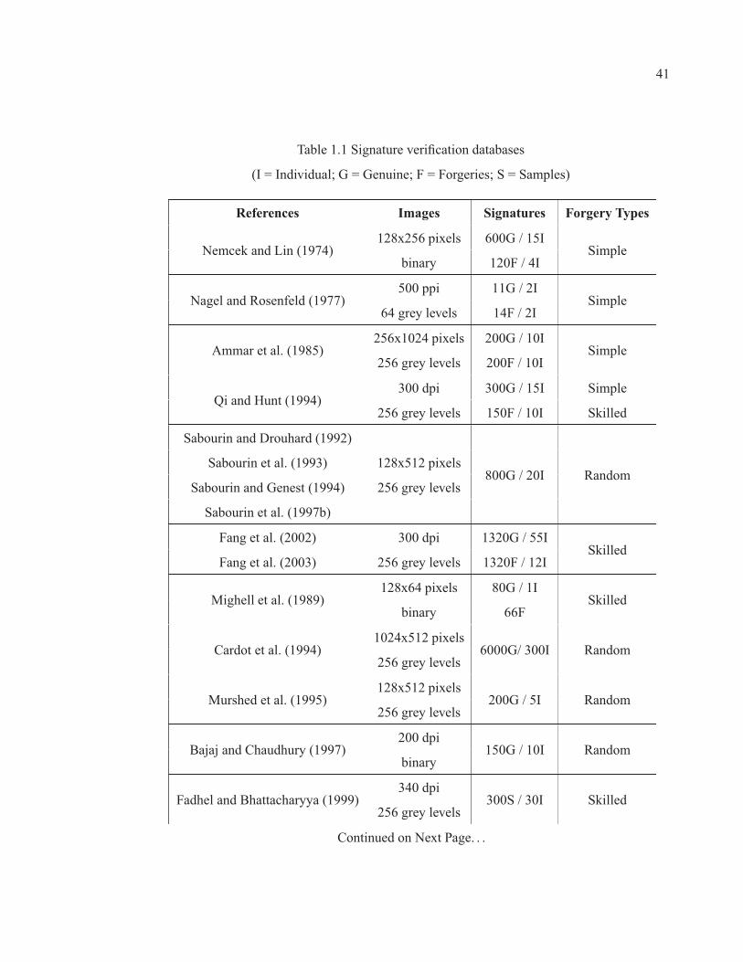
41

Table 1.1 Signature verification databases

(I = Individual; G = Genuine; F = Forgeries; S = Samples)

References Images Signatures Forgery Types

Nemcek and Lin (1974)128x256 pixels 600G / 15I

Simplebinary 120F / 4I

Nagel and Rosenfeld (1977)500 ppi 11G / 2I

Simple64 grey levels 14F / 2I

Ammar et al. (1985)256x1024 pixels 200G / 10I

Simple256 grey levels 200F / 10I

Qi and Hunt (1994)300 dpi 300G / 15I Simple

256 grey levels 150F / 10I Skilled

Sabourin and Drouhard (1992)

800G / 20I RandomSabourin et al. (1993) 128x512 pixels

Sabourin and Genest (1994) 256 grey levels

Sabourin et al. (1997b)

Fang et al. (2002) 300 dpi 1320G / 55ISkilled

Fang et al. (2003) 256 grey levels 1320F / 12I

Mighell et al. (1989)128x64 pixels 80G / 1I

Skilledbinary 66F

Cardot et al. (1994)1024x512 pixels

6000G/ 300I Random256 grey levels

Murshed et al. (1995)128x512 pixels

200G / 5I Random256 grey levels

Bajaj and Chaudhury (1997)200 dpi

150G / 10I Randombinary

Fadhel and Bhattacharyya (1999)340 dpi

300S / 30I Skilled256 grey levels

Continued on Next Page. . .

References Images Signatures Forgery Types

Sansone and Vento (2000)300 dpi 980G / 49I Simple

256 grey levels 980F / 49I Skilled

Blatzakis and Papamarkos (2001) binary 2000G / 115I Random

Quek and Zhou (2002)516x184 pixels 535G / 24I

Skilled256 grey levels 15-20F / 5I

Vélez et al. (2003)300 dpi

112S / 28I not specified256 grey levels

Armand et al. (2006b) not specified936G / 39I

Skilled1170F / 39I

Rigoll and Kosmala (1998) not specified280G / 14I Simple

60F Skilled

Justino (2001) 300 dpi 4000G / 100I Simple

Justino et al. (2005) 256 grey levels 1200F / 10I Skilled

Bertolini et al. (2010)

Coetzer (2005)300 dpi 660G / 22I Simple

binary 264F / 6I Skilled

Deng et al. (1999)600 ppi 1000G / 50I Simple

256 grey levels 2500G / 50I Skilled

Srihari et al. (2004)300 dpi 1320G/ 55I

Skilled256 grey levels 1320F / 55I

Martinez et al. (2004) 300dpi 3840G / 160ISkilled

Ferrer et al. (2005) 256 grey levels 4800F / 160I

Ozgunduz et al. (2005) 256 grey levels 1320S / 70I Skilled

Bastos et al. (1997) not specified 120G / 6I Random

Huang and Yan (2002)100 dpi 1272G / 53I

Skilled256 grey levels 7632F / 53I

42

CHAPTER 2

A MULTI-HYPOTHESIS APPROACH

Though not fully explored in literature, it has recently been shown that the Receiver Operating

Characteristic (ROC) curve – where the True Positive Rates are plotted as function of the False

Positive Rates – provides a powerful tool for evaluating, combining and comparing off-line

SV systems (Coetzer and Sabourin, 2007; Oliveira et al., 2007). Several interesting properties

can be observed from ROC curves. First, Area Under Curve (AUC) is equivalent to the prob-

ability that the classifier will rank a randomly chosen positive sample higher than a randomly

chosen negative sample (Fawcett, 2006). This measure is useful to characterize the system

performance by using a single scalar value. In addition, the optimal threshold for a given class

distribution lies on the ROC convex hull, which is defined as being the smallest convex set con-

taining the points of the ROC curve. Finally, by taking into account several operating points

(thresholds), the ROC curve allows to analyze these systems under different classification costs

(Fawcett, 2006). This property is useful, for instance, for off-line SV systems where the op-

erating points are selected dynamically according to the risk associated with the amount of a

bank check.

In this chapter, an approach based on the combination of classifiers in the ROC space is pro-

posed to improve performance of off-line SV systems designed from limited and unbalanced

data. By training a set of classifiers with different parameters, and then selecting the best classi-

fier(s) for each operating point, it is possible to construct a composite ROC curve that provides

a more accurate estimation of system performance during training and significantly reduces

the error rates during operations. This approach is based on the multiple-hypothesis princi-

ple (Fujisawa, 2007), which request the system to propagate several hypothesis throughout the

recognition steps, generating a hierarchical tree of possible solutions.

Although the proposed approach may be applied to any type of statistical or neural 2-class

classifier, this work involves HMMs trained by using different number of states and different

44

codebooks. In order to avoid the problems caused by the use of limited codebooks, and ensure

that the system can be designed even with a single user, two databases are employed by the pro-

posed approach: the development database (DBdev), which contains the signatures of writers

(not enrolled to the SV system) used to generate the candidate codebooks; and the exploitation

database (DBexp), which contains the signatures of the final users. The latter contains samples

used to train, validate and test HMMs.

The rest of this chapter is organized as follows. The next section presents a brief survey of off-

line SV systems based on discrete HMMs. Section 2.2 describes some key issues that affect the

performance of off-line SV systems. Then, Section 2.4 describes the proposed approach and its

advantages. In Section 2.5, the experimental results are shown and discussed. Finally, Section

2.6 concludes the chapter with a general discussion. The contents of this chapter have been

published as a journal article in (Batista et al., 2010a) and as a conference article in (Batista

et al., 2009).

2.1 Off-line SV systems based on discrete HMMs

A traditional off-line SV system based on discrete HMMs follows the steps shown by Figure

2.1. At first, the signature is scanned in order to obtain a digital representation I(x, y). Af-

ter applying some corrections to the signature image during the pre-processing step (such as

noise removal and centering), a set of feature vectors F = {F1,F2, ...,FL} are extracted and

quantized in a sequence of discrete observations O = {o1, o2, ..., oL}, where each observation

oi is a symbol provided by the codebook and L is the sequence size. Finally, the signature is

classified as genuine or forgery by using the corresponding writer-dependent HMM λ.

Note that Figure 2.1 illustrates a writer-dependent system, where each writer is associated to a

specific HMM trained with his/her corresponding genuine signature samples. Since each writer

is associated with a single HMM, this system is also referred as a single-hypothesis system.

Multi-hypothesis systems, on the other hand, allow a same writer to employ different classifiers

depending on the input samples.

45

Figure 2.1 Block diagram of a traditional off-line SV system based on discrete HMMs.

The rest of this section provides additional details on the feature extraction, vector quantization

and classification sub-systems considered in this work.

2.1.1 Feature Extraction

As described in Chapter 1, two classes of features are used in off-line SV: (i) static, related

to the signature shape and (ii) pseudo-dynamic, related to the dynamics of the writing. These

features can be extracted locally, if the signature is viewed as a set of segmented regions, or

globally, if the signature is viewed as a whole. Since the HMMs are used to model sequence of

observations, the local approach is typically employed (El-Yacoubi et al., 2000; Justino, 2001;

Justino et al., 2000; Rigoll and Kosmala, 1998).

In the grid segmentation scheme of Justino (2001), for instance, the signature images (com-

posed of 400x1000 pixels) are divided in 62 horizontal cells, where each cell is a rectangle

46

composed of 40x16 pixels. To absorb the horizontal variability of the signatures, the blank

cells in the end of the images are discarded. Therefore, the images may have a variable number

of horizontal cells, while the number of vertical cells is always 10. Figure 2.2 shows an exem-

ple of a signature image with its final width. Note that the segmentation can be performed both

in horizontal and vertical directions.

Figure 2.2 Example of grid segmentation scheme.

Each column of cells is then converted into a feature vector, where each vector element contains

the density of pixels in its respective cell. In other words, each vector element is a value

between 0 and 1 which corresponds to the number of black pixels in a cell divided by the total

number of pixels of this cell. Therefore, the preprocessed signature I ′(x, y) is represented by

a set of feature vectors F = {Fj} , 1 ≤ j ≤ col, where col is the number of columns in the

grid. Other static features, such as pixel distribution and gravity center, as well as pseudo-

dynamic features, such as axial slant and stroke curvature, have been extracted through this

segmentation scheme (Justino, 2001; Justino et al., 2005).

47

2.1.2 Vector Quantization

In order to generate a sequence of discrete observations, each extracted feature vector is quan-

tized as one of the previously-computed symbols of the codebook. The codebook may be

generated through an iterative clustering algorithm called K-means (Makhoul et al., 1985). As

explained by Algorithm 2.1, the feature vectors F = {Fj} , 1 ≤ j ≤ col, are separated into N

clusters Ui, 1 ≤ i ≤ N , where each cluster Ui represents a symbol in the the codebook.

Inputs:– the set of feature vectors, F = {Fj} , 1 ≤ j ≤ col– the number of centroids/clusters, NOutputs: the set of updated centroids, centi, 1 ≤ i ≤ N ,

1: from the set of feature vectors F , choose an initial set of N centroids centi2: classify the feature vectors into the clusters Ui by using the nearest neighbor rule:

Fj ∈ Ui, iff dist(Fj , centi) ≤ dist(Fj , centk), k �= j, 1 ≤ k ≤ N

3: update the centroid of each cluster by averaging its corresponding feature vectors4: if the centroids have changed then5: go to step 26: end if

Algorithm 2.1 K-means algorithm, where Ui is the ith cluster with centroid centi.

2.1.3 Classification

Once the sequences of discrete observations are obtained, they are used to train and test the

HMMs. A discrete HMM λ can be defined as λ = (S,M,A,B, π), where (Rabiner, 1989):

1) S is the number of distinct states in the model. The set of states is denoted by S =

{S1, S2, ..., SS}, and st is the state at time t;

2) M is the alphabet size, that is, the number of distinct observation symbols per state. The set

of symbols is denoted by V = {v1, v2, ..., vM};

48

3) A is the state transition probability distribution, denoted by A = {aij}, where

aij = P [st+1 = Sj |st = Si], and 1 ≤ i, j ≤ S;

4) B is the observation symbol probability distribution, denoted by B = {bj(k)}, where

bj(k) = P [vk at t|st = Sj ], and 1 ≤ k ≤M, 1 ≤ j ≤ S;

5) and π is the initial state distribution, denoted by π = {πi}, where πi = P [s1 = Si], and

1 ≤ i ≤ S.

HMMs can be classified in two main types of topologies (Rabiner, 1989): the ergotic and the

left-to-right topologies, as depicted by Figure 2.3. The ergotic topology is a specific case of

a fully-connected model in which every state can be reached from any other state in a finite

number of steps. With the left-to-right topology, the state indices increase from left to right

(that is, aij = 0, j < i), and no transitions are allowed to states whose indices are lower

than the current state. As consequence, the sequence of observations must begin in S1 (that

is, πi = 0 when i �= 1, and πi = 1 when i = 1) and must end in SN . Often, the additional

constraint aij = 0, j > i + Δ is used, where Δ is a value used as the limit of jumps. For

instance, the left-to-right model illustrated in Figure 2.3 (b) has Δ = 2, which forbids jumps

with more than 2 states.

(a) (b)

Figure 2.3 Examples of (a) 4-state ergodic model and (b) 4-state left-to-right model.Adapted from Rabiner (1989)

49

Given a model initialized according to the constraints described so far, there are three tasks of

interest (Huang et al., 2001):

1) The Evaluation Problem. Given a model λ and a sequence of observationsO = {o1, o2, ..., oL},

what is the probability of the model λ has generated the observation O, that is, P (O|λ);

2) The Decoding Problem. Given a model λ, what is the most likely sequence of states S =

{S1, S2, ..., SS} in the model that produces the sequence of observationsO = {o1, o2, ..., oL};

3) The Learning Problem. Given a model λ and a sequence of observationsO, how the model

parameters can be adjusted so as to maximize the probability P (O|λ).

An advantage of the discrete HMMs is that it is not necessary to have a priori knowledge

about the probability distributions to model a signal (Britto, 2001). With enough representative

training data, it is possible to adjust the parameters for the HMM. Algorithms based on the

expectation-maximization (E-M) technique (e.g., the Baum-Welch algorithm) are generally

used to perform this task (Gotoh et al., 1998).

Typically, only genuine signatures are used for training an user-specific HMM for SV. In this

case, the decision boundary between impostor and genuine spaces is defined by using a val-

idation set that contains samples of both classes. Another particularity of HMM-based SV

systems is the use of the left-to-right topology. Indeed, this topology is perfectly adapted to

the dynamic characteristics of the occidental handwritten, in which the hand movements are

always from left to right.

2.2 Challenges with the Single-Hypothesis Approach

In this work, it is assumed that the performance of the whole SV system is measured by an

overall ROC curve obtained from a set of user-specific ROC curves. Averaging methods have

been used to group ROC curves produced from different user-specific classifiers in single-

hypothesis systems (Fawcett, 2006; Jain and Ross, 2002).

50

Jain and Ross (2002), for instance, proposed a method to generate an averaged ROC curve

taking into account user-specific thresholds1. For each user i, the cumulative histogram of

his/her random forgery scores (taken from a validation dataset) is computed. Then, the scores

providing a same value of cumulative frequency, γ, are used as thresholds to compute the

operating points {TPRi(γ), FPRi(γ)}. Finally, the operating points associated with a same

γ (and related to different users) are averaged. Note that γ can be viewed as the True Negative

Rate (TNR) (i.e., ratio of random forgeries correctly classified to the total of random forgeries)

and that it may be associated with different thresholds. Fig. 2.4 shows an example where the

thresholds associated with γ = 0.3 are different for users 1 and 2, that is τuser1(0.3) ∼= −5.6

and τuser2(0.3) ∼= −6.4.

−8 −7 −6 −5 −4 −3 −20

0.1

0.2

0.3

0.4

0.5

0.6

0.7

0.8

0.9

1

Random Forgery Scores (τ)

Cum

ulat

ive

Fre

quen

cy (γ

)

user 1user 2

Figure 2.4 Cumulative histogram of random forgery scores regarding two different usersin a single-hypothesis system. The horizontal line indicates that γ = 0.3 is associated to

two different thresholds, that is, τuser1(0.3) ∼= −5.6 and τuser2(0.3) ∼= −6.4.

1Since biometric systems typically use a common threshold across users, Jain and Ross (Jain and Ross, 2002)have shown that it is possible to improve system performance by setting user-specific thresholds.

51

In off-line SV, where the dataset used to model a writer generally contains a reduced number

of genuine samples against several random forgeries, it is common to obtain ROC curves with

concave areas. In general, a concave area indicates that the ranking provided by the classifier in

this region is worse than random (Flach and Wu, 2003). Figure 2.5 shows an example of score

distribution in an off-line SV system. The positive class, P, contains only 10 genuine samples

of a given writer, while the negative class, N, contains 100 samples of forgeries.

−15 −10 −5 0 5 10 150

1

2

3

4

5

6

Similarity Score

Freq

uenc

y

NP

Figure 2.5 Typical score distribution of a writer, composed of 10 positive samples(genuine signatures) vs. 100 negative samples (forgeries).

Due to the limited amount of samples in the positive class, the resulting ROC curve (see Fig-

ure 2.6) presents three concave areas, which correspond to low-quality predictions (Flach and

Wu, 2003). For example, the similarity scores between −1.2 and 0 provide TPRs of 90%.

The result of averaging the ROC curves related to the models of 100 different writers, by us-

ing the Ross’s method, is illustrated by Figure 2.7. Note that the imperfections of individual

52

ROC curves are hidden within the average points, which can be observed with any averaging

algorithm.

0 0.2 0.4 0.6 0.8 1

0.4

0.5

0.6

0.7

0.8

0.9

1

FPR

TPR concavity produced by

similarity scores between −1.2 and 0

Figure 2.6 ROC curve with three concavities.

The drawback of using an averaged ROC curve can be observed during the selection of optimal

thresholds in the respective convex hull. Given two γ in the convex hull, γ1 and γ2, where each

one minimizes a different set of costs (Tortorella, 2005), γ2 should provide a TPR higher than

γ1 whenever γ1 > γ2. However, regarding a user-specific ROC curve, γ1 and γ2 may fall

in a same concave area, providing identical TPRs. An example is illustrated by Figure 2.7,

where TPR(γ = 0.86) is higher than TPR(γ = 0.91) in the global convex hull, but, in the

user-specific ROC curve, TPR(γ = 0.86) is equal to TPR(γ = 0.91).

53

0 0.05 0.1 0.15 0.2 0.25 0.3 0.35

0.4

0.5

0.6

0.7

0.8

0.9

1

FPR

TPR

User−specific ROC curve Averaged ROC curve

γ = 0.91γ = 0.86

Global convex hull

Figure 2.7 Averaged ROC curve obtained by applying the Ross’s method to 100 differentuser-specific ROC curves.The global convex hull is composed of a set of optimal

thresholds that minimize different classification costs. However, these thresholds may fallin concave areas of the user-specific ROC curves, as indicated by γ = 0.91 and γ = 0.86.

2.3 The Multi-Hypothesis Approach

Based on the combination of HMMs trained with different number of states, the approach

proposed in this section provides a solution to repair concavities of user-specific ROC curves

while generating a high quality averaged ROC curve. The utilization of different HMMs is

motivated by the fact that the superiority of a classifier over another may not occur on the

whole ROC space (Fawcett, 2006). Indeed, in off-line SV systems where the optimal number

of states for a HMM is found empirically by a cross-validation process2, it is often observed that

the best HMM is not superior than the other intermediate/ sub-optimal HMMs in all operating

points of the ROC space. Three steps are involved in the proposed multi- hypothesis approach:

model selection, combination and averaging.2Given a set of HMMs trained with different number of states, the cross-validation process selects the HMM

providing the highest training probability (Justino et al., 2001; El-Yacoubi et al., 2000).

54

2.3.1 Model Selection

This step allows to select the best classifier for each operating point such that every writer’s

performance is optimized. In this work, a ROC outer boundary is constructed for each writer

in order to encapsulate the best operating points provided by multiple HMMs, each one trained

by using a different number of states. Given a set of ROC curves generated from different

classifiers associated with a same writer, the process consists in splitting the x axis ∈ [0, 1] into

a number of bins, and within each bin finding the pair (FPR, TPR) having the largest value

of TPR. While the ROC outer boundary is being generated, the best model HMMj , where j

is the number of states, is automatically chosen for each operating point. Figure 2.8 shows an

example of a user-specific ROC outer boundary constructed from ROC curves of two different

classifiers, HMM7 and HMM9. The corresponding convex hull is composed of three vertices,

p, q and r, where p and q are associated with HMM9, and r is associated with HMM7.

0 0.2 0.4 0.6 0.8 10

0.1

0.2

0.4

0.5

0.6

0.7

0.8

0.9

1

FPR

TPR

ROC HMM9

ROC HMM7

r

q

pConvex Hull

ROC outer boundary

Figure 2.8 ROC outer boundary constructed from ROC curves of two different HMMs.Above TPR = 0.7, the operating points are taken from HMM7, while below

TPR = 0.7, the operating points correspond to HMM9.

55

Algorithm 2.2 presents the approach for generating the outer boundary of ROC curves pro-

duced by training Lmin HMMs on a same dataset but with different number of states; where

Lmin is the number of observations in the shorter training sequence.

Inputs: the training and validation setsOutputs: the set of ROC outer boundaries

1: for each writer i = 1, 2, ..., M do2: for each number of states j = 2, 3, ..., Lmin do3: train an HMM with j states4: calculate the ROC curve j by using the validation set5: end for6: for each bin k ∈ [0, 1] do7: let λ(k) be the classifier associated to the current bin8: set TPR(k) ← 09: for each ROC curve j do

10: if TPRj(k) > TPR(k) then11: TPR(k) ← TPRj(k)12: FPR(k) ← FPRj(k)13: λ(k) ← HMMj(k)14: end if15: end for16: end for17: use the pairs {FPR(k), TPR(k)} to generate the ROC outer boundary i18: end for

Algorithm 2.2 Generating ROC outer boundaries from different HMMs.

Note that this process can also be extended for multiple codebooks. In other words, by train-

ing an ensemble of HMMs with different codebook sizes and different number of states, each

bin can be associated with the pair {codebook, state} providing the highest TPR. Therefore,

depending on the operating point, a same individual may use a different model, denoted as

HMMNj , trained with j states and with a codebook of N clusters.

56

2.3.2 Combination

This step allows to interpolate between two consecutive classifiers on the ROC curve in order

to obtain not yet reached operating points. In this work, the method proposed by Scott et. al

(Scott et al., 1998) is applied to the ROC outer boundaries in order to repair concavities. Given

two vertices A and B on the convex hull, it is possible to realize a point C, located between A

and B, by randomly choosing A or B. The probability of selecting one of the two operating

points is determined by the distance of C regarding A and B (see Equations 2.1 and 2.2).

The expected operating point (FPRC , TPRC) is given by Equations 2.3 and 2.4 (Scott et al.,

1998).

P(C = A) = (FPRC−FPRB)/(FPRA−FPRB) (2.1)

P(C = B) = 1−P(C = A) (2.2)

FPRC = (P(C = A)·FPRA)+(P(C = B)·FPRB) (2.3)

TPRC = (P(C = A)·TPRA)+(P(C = B)·TPRB) (2.4)

By using the Equations 2.1 to 2.4, Algorithm 2.3 can realize any FPRC located between two

consecutive classifiers, A and B, where each classifier corresponds to a hull vertex of a user-

specific ROC outer boundary. Figure 2.9 presents an example of a maximum realizable ROC

(MRROC) curve.

2.3.3 Averaging

Finally, a process based on the Jain and Ross’s method (Jain and Ross, 2002) is used to group

the operating points already computed during the combination step. Given a γ, the Algorithm

2.4 searches the pairs {TPRi(γ), FPRi(γ)} where FPRi(γ) = 1− γ (recalling that γ can be

57

0 0.2 0.4 0.6 0.8 10.82

0.84

0.86

0.88

0.9

0.92

0.94

0.96

0.98

1

1.02

FPR

TPR

MRROC curveROC curve

A

B

C*

Figure 2.9 Example of MRROC curve. By using combination, any operating point Cbetween A and B is realizable. In this example, for a same FPR, the TPR associated

with C could be improved from 90% to 96%.

viewed as the TNR). Then, the operating points corresponding to a same γ are averaged and

used to generate the averaged ROC curve.

2.3.4 Testing

During operations, γ is used to retrieve the set of user-specific HMMs/thresholds which will be

applied on input samples. Figure 2.10 illustrates two possible situations linking the averaged

ROC curve and a user-specific MRROC curve. In the first case, γ falls directly on HMM7.

Thus, the user-specific threshold associated to this γ will be used to classify the input samples.

In the second case, the requested γ is obtained by combining classifiers HMM7 and HMM9.

That is, each test sample must be randomly assigned to either HMM7 or to HMM9, according

to the probabilities given by Equations 2.1 and 2.2. Note that a test sample is not assigned to

both classifiers at the same time. However, if a fusion strategy is incorporated to the process,

58

Inputs: the set of ROC outer boundariesOutputs: the set of MRROC curves

1: for each writer i = 1, 2, ..., M do2: for each FPRC ∈ [0, 1] do3: find, in the convex hull of his/her ROC outer boundary, the pair of classifiers (A, B)

able to realize FPRC

4: calculate:5: //the probability of A to be chosen (Eq. 2.1):

P(A) ←(FPRC − FPRi(B))

(FPRi(A) − FPRi(B))

6: //the probability of B to be chosen (Eq. 2.2):

P(B) ← 1 −P(A)

7: //the expected operating points (Eqs. 2.3 and 2.4):

FPRC ← (P(A) · FPRi(A)) + (P(B) · FPRi(B))

TPRC ← (P(A) · TPRi(A)) + (P(B) · TPRi(B))

8: end for9: use the pairs {FPRC, TPRC} to generate the MRROC curve i

10: end for

Algorithm 2.3 Generating MRROC curves.

there are no restrictions to combine the decisions of both classifiers.

2.4 Experimental Methodology

Two types of codebook have been employed in off-line SV systems based on discrete HMMs:

the universal codebook, shared by all writers enrolled to the system, and the user-specific

codebook, adapted to a particular writer. However, as discussed before, these codebooks have

typically been constructed by using the same data that are used to train the HMMs (Ferrer et al.,

2005; Rigoll and Kosmala, 1998). Instead, this section investigates the use of an independent

SV database to generate universal and user-specific codebooks. In both cases, the impact of

applying the multi-hypothesis approach to improve the system performance is analysed.

59

Inputs: the set of MRROC curvesOutputs: the averaged ROC curve

1: for each value of γ ∈ [0, 1] do2: set {FPR(γ), TPR(γ)} ← 03: for each writer i = 1, 2, ..., M do4: find, in his/her MRROC curve, the operating point associated with γ, that is:

{FPRi(γ), TPRi(γ)} |FPRi(γ) = 1 − γ

5: update FPR(γ) and TPR(γ) as:

FPR(γ) ← FPR(γ) + FPRi(γ)

TPR(γ) ← TPR(γ) + TPRi(γ)

6: end for7: divide FPR(γ) and TPR(γ) by the number of writers M :

FPR(γ) ← FPR(γ)/M

TPR(γ) ← TPR(γ)/M

8: end for9: use the pairs {FPR(γ), TPR(γ)} to generate the averaged ROC curve

Algorithm 2.4 Generating the averaged ROC curve.

Averaged ROC curve User-specific MRROC curve

HMM 9

HMM 7

HMM 7

HMM 7

HMM 7

HMM 9

Figure 2.10 Retrieving user-specific HMMs from an averaged ROC curve.

60

The Brazilian signature database from PUCPR (Pontifícia Universidade Católica do Paraná)

(Batista et al., 2010a, 2009; Bertolini et al., 2010; Justino et al., 2000), is used for proof-of-

concept computer simulations. It contains 7920 samples of signatures that were digitized as

8-bit greyscale images over 400x1000 pixels, at resolution of 300 dpi. The signatures were

provided by 168 writers and are organized as follows:

1) The development database (DBdev). DBdev is composed of 4320 genuine samples sup-

plied by 108 writers, and is mostly used to construct universal codebooks. For each writer,

there are 20 genuine samples for training, 10 genuine samples for validation and 10 genuine

samples for test.

2) The exploitation database (DBexp). DBexp contains 60 writers, each one with 40 samples

of genuine signatures, 10 samples of simple forgery and 10 samples of skilled forgery. For

each writer, 20 genuine samples are used for training, 10 genuine samples for validation,

and 30 samples for test (10 genuine samples, 10 simple forgeries and 10 skilled forgeries).

Moreover, 10 genuine samples are randomly selected from the other 59 writers and used

as random forgeries to test the current model. For ROC analysis, we use 10 genuine sam-

ples (from validation) versus 1080 random forgeries taken from DBdev (i.e., 10 validation

samples from 108 writers).

Given DBdev and DBexp, two experiments are performed:

1) Off-line SV based on an universal codebook. As proposed by Justino et al. (2000), an eval-

uation system is generated with DBdev by trying different candidate codebooks obtained

from this same dataset. Then, the codebook which performs the best in DBdev is selected to

develop the final system, that is, a system for the writers in DBexp. This strategy assumes

that if DBdev is representative of the whole population, the codebook selected to represent

this database will also work well for DBexp.

2) Off-line SV based on user-specific codebooks. By using the same candidate codebooks of

the previous experiment, the idea is to find, for each writer in DBexp, the codebook which

61

the best adapts to his/ her individual characteristics. Thus, a same off-line SV system may

work with multiple codebooks.

Therefore, while DBdev is used to construct codebooks, as well as to develop evaluation SV

systems, a DBexp is employed for training, testing and validation of the final SV system. As

mentioned, the use of DBdev allows to construct codebooks earlier, with enough data, indepen-

dently of the writers in DBexp.

The greyscale signature images are converted to black and white using the Otsu’s binarization

method (Gonzalez and Woods, 2002). Then, they are represented by means of density of

pixels, extracted through the same grid resolution described in Section 2.1. By trying different

resolutions, Justino (2001) showed that the grid with 10 vertical cells (where each cell is a

rectangle composed of 40x16 pixels) is the most suitable for the Brazilian SV database. This

analysis was performed with DBdev, that is, using signature samples from writers not enrolled

to the system.

By varying the number of clusters from 10 to 150, in steps of 5, 29 candidate codebooks

are obtained; where each one is constructed by using the first 30 signatures (training set +

validation set) of each writer in DBdev. In the first experiment, in order to select the universal

codebook, an averaged ROC curve is produced for each different version of the evaluation

system. Then, the codebook providing the averaged ROC curve with highest AUC is chosen. In

the second experiment, the user-specific codebooks are selected before the averaging step; that

is, by choosing the codebook providing the MRROC curve with highest AUC for each writer.

Then, the individual MRROC curves are averaged. Since high values of FPR are rarely useful

in real situations, the AUC may be calculated regarding a specific region of interest of the ROC

space.

After codebook selection, an off-line SV system is designed for each writer enrolled to the

system (i.e., using DBexp). In the first experiment, a ROC outer boundary is obtained for

each writer by using the same universal codebook and a set of HMMs trained with a different

number of states. In the second experiment, a ROC outer boundary is obtained for each writer

62

by using his/her own codebook and a set of HMMs trained with a different number of states.

Note that, in both experiments, the ROC curves are generated by using a validation set which

contains only genuine samples and random forgeries.

Each HMM is trained by using the Baum-Welch forward-backward algorithm (Rabiner, 1989),

and at each iteration t, a error measure Et is calculated as:

Et = P(O/λ(t))−P(O/λ(t−1))P(O/λ(t))+P(O/λ(t−1))

(2.5)

where P(O/λ(t)) and P(O/λ(t−1)) represent the joint probabilities of the training sequences

O have been generated by the HMM λ in the instants t and t − 1, respectively. The goal is to

reach an error of 10−5 or smaller (Justino, 2001). Besides this stop criteria, the validation set

is used in order to select the optimal training point before overfitting.

2.5 Simulation Results and Discussions

2.5.1 Off-line SV based on an universal codebook

In a first step, the multi-hypothesis approach (Algorithms 2.2 to 2.4) was applied for each one

of the candidate codebooks by using the whole validation set. Among the 29 averaged ROC

curves, the codebook of 35 clusters (CB35) provided the highest AUC (i.e., 0.997). Figure 2.11

shows the averaged ROC curve and AUC associated with CB35. Then, in order to confirm this

result, 10 different averaged ROC curves were generated for each codebook by randomly se-

lecting a subset of signatures in the validation set. Since there are much more random forgeries

than genuine samples, only the forgery space was changed for each averaged ROC curve.

Figure 2.12 presents the relation between the Number of Clusters (NC) used in each code-

book and the corresponding AUC, calculated on the entire averaged ROC space. This graphic

confirms that the codebook with 35 clusters provides the highest AUCs for this population.

Moreover, the Kruskal-Wallis test (Gibbons, 1985) indicates that the AUC values correspond-

ing to CB35 are significantly different to the data regarding any other codebook in the graphic.

63

0 0.2 0.4 0.6 0.8 1

0.8

0.82

0.84

0.86

0.88

0.9

0.92

0.94

0.96

0.98

1

FPR

TPR

CB35

AUC = 0.997

Figure 2.11 Composite ROC curve, with AUC = 0.997, provided by CB35 on the wholevalidation set of DBdev.

The next step consisted of applying the codebook CB35 to DBexp, which is composed of 60

writers. As expected, CB35 also performed well for this population, providing an AUC of

0.998 in the region of interest (i.e., between FPR = 0 and FPR = 0.1) of the averaged ROC

space. The ROC curve of the multi-hypothesis system is indicated by the star-dashed line in

Figure 2.13. Whereas the circle-dashed line represents the baseline or single-hypothesis system

used for comparisons. In this system, only the HMM which performs the best in the cross-

validation process (Justino et al., 2001; El-Yacoubi et al., 2000) is considered for generating a

user-specific ROC curve. This means that all operating points of an individual ROC curve are

associated with a same HMM. Moreover, the user-specific ROC curves are directly averaged,

without repairing, by using the standard Ross’s method (Jain and Ross, 2002) (see the inner

graphic in Figure 2.13). As expected, the multi-hypothesis system provided a higher ROC

curve, and, due to the Scott’s method (Scott et al., 1998), a superior number of operating points

was obtained.

64

10 35 60 85 110 1350.975

0.978

0.981

0.984

0.987

0.99

0.993

0.996

0.999

AUC

NC

Outliers+

Figure 2.12 AUC (area under curve) vs NC (number of clusters). As indicated by thearrow, CB35 represents the best codebook for DBdev over 10 averaged ROC curves

generated with different validation subsets of DBdev.

Depending on the operating point, a same writer could employ a different HMM, as shows

Figure 2.14. It is worth noting that the complexity of the HMMs increases with the value of γ;

which indicates that the operating points in the best region of the ROC space (i.e., the upper-left

part) are achieved with a greater number of states.

Figure 2.15 shows the user-specific MRROC curves of two writers. While writer 1 employs

different HMMs in the MRROC space, writer 3 uses the same HMM in all operating points.

The fact that writer 3 obtained AUC=1 by using an HMM with only 2 states (i.e., HMM2)

indicates that his/her corresponding genuine and forgery spaces in the validation set are easily

separable. In other words, high inter-class variability demands less complex models.

In the following phase, the operating points of the averaged ROC space (given by γ) were used

to retrieve the user-specific HMMs/thresholds, and apply them to the test set. Table 2.1 presents

the test set error rates for some γ values in both baseline and proposed systems. In order to ob-

65

0 0.02 0.04 0.06 0.08 0.100.85

0.9

0.95

1

FPR

TPR

Multi−hypothesis system

Single−hypothesis system

0 0.02 0.04 0.06 0.08 0.10

0.2

0.4

0.6

0.8

1

Standard Ross’saveraging method

60 user−specific ROCcurves non−repaired

Figure 2.13 Averaged ROC curves when applying CB35 to DBexp. Before using theRoss’s averaging method, the proposed system used the steps of model selection andcombination in order to obtain smoother user-specific ROC curves; while the baselinesystem directly averaged the 60 user-specific ROC curves, as shows the inner figure.

serve the impact on system performance at each step of the multi-hypothesis approach, results

are first shown without the combination step (that is, by performing model selection followed

by averaging), while the last results correspond to the whole multi-hypothesis approach. Since

there are three types of forgeries in the test set, the average error rate is calculated as

AER(γ) = (FNR(γ)+FPR(γ)rand+FPR(γ)simp+FPR(γ)skil)/4 (2.6)

Which is equivalent to consider equal a priori probabilities, that is, P (genuine) = P (random)

= P (simple) = P (skilled) = 0.25, since the test set of each writer is composed of 10 samples

per category of signature.

66

0 10 20 30 40 50 600

5

10

15

20

25

30

35

40

45

50

55

Writer

Num

ber o

f Sta

tes

γ = 1

(a)

0 10 20 30 40 50 600

5

10

15

20

25

30

35

40

45

50

55

Writer

Num

ber o

f Sta

tes

γ = 0.850

(b)

0 10 20 30 40 50 600

5

10

15

20

25

30

35

40

45

50

55

Writer

Num

ber o

f Sta

tes

γ = 0.700

(c)

0 10 20 30 40 50 600

5

10

15

20

25

30

35

40

45

50

55

Writer

Num

ber o

f Sta

tes

γ = 0.550

(d)

Figure 2.14 Number of HMM states used by different operating points in the averagedROC space. The complexity of the HMMs increases with the value of γ, indicating thatthe operating points in the upper-left part of the ROC space are harder achieved. In other

words, the best operating points are achieved with more number of states.

In general, the multi-hypothesis system provided smaller error rates. Moreover, the FPR(γ)rand

are closer to the expected error rates given by 1-γ (recalling that γ can be viewed as the TNR,

and that FPR = 1− TNR). Additional results obtained with the multi-hypothesis system are

presented in Table 2.2.

In order to analyze the impact of repairing individual ROC curves, the proposed approach was

applied only to the 20 writers having ROC curves with concavities. On average, 75.91% of the

67

0 0.1 0.2 0.3 0.4 0.5

0.8

0.85

0.9

0.95

1

FPR

TPR

data1data2data3data4data5data6Writer 3Writer 1

Writer 1: HMM17

Writer 3: HMM2 for all γ

Writer 1: HMM7

Writer 1: HMM11

Figure 2.15 User-specific MRROC curves of two writers in DBexp. While writer 1 canuse HMMs with 7, 11, or 17 states depending on the operating point, writer 3 employs the

same HMM all the time. Note that writer 3 obtained a curve with AUC = 1, whichindicates a perfect separation between genuine signatures and random forgeries in the

validation set.

problematic writers had their AERs on test enhanced with the multi-hypothesis system in the

region between γ = 0.9 and γ = 1; while 18.64% performed better with the single-hypothesis

system. For the remaining 5.45%, both systems performed equally. Figure 2.16 presents the

results for some γ values, where the improvements obtained with the multi-hypothesis system

are located in the positive side, that is, below the dotted line. For instance, with the single-

hypothesis system, the writer indicated by the arrow in (a) had an AER of 22.5%. When using

the multi-hypothesis system, the respectiveAER was reduced to 4.9%, that is, 17.6% lower.

Finally, the multi-hypothesis system required fewer HMM states than the single-hypothesis

system. Figure 2.17 shows the number of HMM states used by each writer in the single-

hypothesis system. Note that these models, applied to all operating points, are more complex

than those ones previously shown in Figure 2.14. Regarding the entire ROC space, the pro-

68

Table 2.1 Error rates (%) on test

Single-hypothesis systemγ FNR FPRrandom FPRsimple FPRskilled AER

0.96 0.50 6.00 10.83 64.83 20.540.97 0.83 5.67 9.00 60.17 18.920.98 1.17 4.00 5.67 52.50 15.830.99 2.33 2.67 4.00 42.67 12.92

1 12.67 0.33 1.17 19.83 8.50Multi-hypothesis system without combination

γ FNR FPRrandom FPRsimple FPRskilled AER0.96 3.17 5.17 11.00 62.33 20.420.97 3.33 4.17 9.33 58.50 18.830.98 3.83 1.83 6.67 51.17 15.880.99 5.00 1.17 4.17 41.17 12.88

1 12.83 0.33 1.17 20.50 8.71Multi-hypothesis system

γ FNR FPRrandom FPRsimple FPRskilled AER0.96 4.13 4.67 8.70 54.81 18.070.97 4.15 3.17 7.35 52.23 16.720.98 4.48 2.50 5.51 47.05 14.880.99 5.55 1.17 4.00 39.63 12.58

1 12.83 0 1.17 20.50 8.62

Table 2.2 Additional error rates (%) on test obtained with the multi-hypothesis system

γ FNR FPRrandom FPRsimple FPRskilled AER0.991 5.71 1.00 3.83 38.01 12.130.992 5.81 0.67 3.83 37.38 11.920.993 6.00 0.67 3.50 36.15 11.580.994 6.17 0.67 3.50 35.90 11.560.995 6.30 0.67 3.17 34.80 11.230.996 7.10 0.67 2.67 33.73 11.040.997 7.63 0.67 2.67 32.48 10.860.998 8.21 0.67 2.67 30.60 10.540.999 9.37 0.17 1.91 26.83 9.57

1 12.83 0 1.17 20.50 8.62

posed approach reduced by 48.09% the number of states employed by the HMMs. This occurs

because during the model selection step (see Algorithm 2.2), when two or more HMMs achieve

the same TPR, the model with fewer states is chosen.

69

0 5 10 15 20 25 30 350

5

10

15

20

25

30

35γ = 0.96

AER (%) single−hypothesis system

AE

R (%

) mul

ti−hy

poth

esis

sys

tem

−

+

(a)

0 5 10 15 20 25 30 350

5

10

15

20

25

30

35γ = 0.97

AER (%) single−hypothesis system

AE

R (%

) mul

ti−hy

poth

esis

sys

tem

−

+

(b)

0 5 10 15 20 25 30 350

5

10

15

20

25

30

35γ = 0.98

AER (%) single−hypothesis system

AE

R (%

) mul

ti−hy

poth

esis

sys

tem

+

−

(c)

0 5 10 15 20 25 30 350

5

10

15

20

25

30

35γ = 0.99

AER (%) single−hypothesis system

AE

R (%

) mul

ti−hy

poth

esis

sys

tem

−

+

(d)

Figure 2.16 User-specific AERs obtained on test with the single- and multi-hypothesissystems. The stars falling below the dotted lines represent the writers who improved their

performances with multi-hypothesis system.

2.5.2 Off-line SV based on user-specific codebooks

This experiment explored the idea of using user-specific codebooks in order to reduce indi-

vidual error rates. Since each writer must be evaluated separately, the selection of the best

user-specific codebook was performed after the combination step, by choosing that one pro-

viding the MRROC curve with greatest AUC in the region of interest (i.e., between FPR = 0

and FPR = 0.1). Figure 2.18 (a) presents the codebook selected for each writer. For some

70

0 10 20 30 40 50 600

5

10

15

20

25

30

35

40

45

50

55

Writer

Num

ber o

f Sta

tes

Figure 2.17 Number of HMM states selected by the cross-validation process in thesingle-hypothesis system. These models are used in all operating points of the ROC space.

writers, due to the high variability inter-class on validation (i.e., genuine signatures versus ran-

dom forgeries), all codebooks provided AUC = 1. In these cases, the universal codebook CB35,

found in the previous experiment, was used. Figure 2.18 (b) indicates that only 13 codebooks

(out of 29) were selected by this experiment; where 58% of the writers used the universal

codebook CB35, and 15% used a codebook with 150 clusters.

After selecting the best codebook per user, the user-specific MRROC curves were averaged

by using Algorithm 2.4. The dash-dot line in Figure 2.19 shows the resulting averaged ROC

curve (AUC = 0.9989), which is better than the curve obtained with the previous version of

multi-hypothesis system (i.e., with CB35) in the region between γ = 0.995 and γ = 1. This

improvement was also observed on test, as shows Table 2.3; specially for γ = 1. The results

for γ = 0.96 to 0.99 are not shown in Table 2.3 since both systems performed similarly for

γ < 0.995. Figure 2.20 presents the AERs of the 20 problematic writers obtained with the

two multi-hypothesis systems. On average, 36.25% of these writers had their AERs enhanced

71

0 10 20 30 40 50 600

20

40

60

80

100

120

140

160

Writer

NC

(a)

58%

15%

NC = 35

NC = 150

(b)

Figure 2.18 (a) Distribution of codebooks per writer. In the cases where all codebooksprovided AUC = 1, the universal codebook CB35 was used. (b) Among the 13 codebooksselected by this experiment, CB35 was employed by 58% of the population, while 15% of

the writers used a codebook with 150 clusters.

with the use of user-specific codebooks. This represents 12.08% of the whole population,

which may indicate a considerable amount of users in a real world application. Only 16.25%

performed better with CB35; and for the remaining 47.50%, both systems performed equally.

Table 2.3 Error rates (%) on test

Results obtained with the multi-hypothesis system when using user-specific codebooksγ FNR FPRrandom FPRsimple FPRskilled AER

0.995 5.93 1.00 3.22 35.10 11.310.996 6.60 0.83 2.85 33.15 10.860.997 6.87 0.67 2.83 31.82 10.550.998 7.73 0.67 2.60 29.22 10.050.999 8.63 0.17 1.60 26.00 9.10

1 9.83 0 1.00 20.33 7.79Results obtained with the multi-hypothesis system when using CB35

γ FNR FPRrandom FPRsimple FPRskilled AER0.995 6.30 0.67 3.17 34.80 11.230.996 7.10 0.67 2.67 33.73 11.040.997 7.63 0.67 2.67 32.48 10.860.998 8.21 0.67 2.67 30.60 10.540.999 9.37 0.17 1.91 26.83 9.57

1 12.83 0 1.17 20.50 8.62

72

0 0.01 0.02 0.03 0.04 0.050.85

0.9

0.95

1

FPR

TPR

Single−hypoth. system using CB35

Multi−hypoth. system using CB35

Multi−hypoth. system usinguser−specific codebooks

γ = 1

{writer, codebook, HMM, threshold}

{writer, HMM, threshold}

{writer, threshold}

γ = 0.995

γ = 0.9

Figure 2.19 Averaged ROC curves obtained for three different systems, where themulti-hypothesis system with user-specific codebooks provided the greatest AUC. While

the single-hypothesis system stores only the user-specific thresholds in the operatingpoints, the multi-hypothesis systems can store information about user-specific thresholds,

classifiers and codebooks in each operating point of the composite ROC curve.

Besides being used to retrieve the set of user-specific classifiers and thresholds, the operating

points of the last multi-hypothesis system also stores information about what codebook to use;

taking into account that a same codebook may be shared by different writers. In the single-

hypothesis system, on the other hand, only the user-specific thresholds are stored, since each

writer employs his/her single classifier in all operating points. It is worth noting that another

variation of the proposed system could be developed by finding the best codebook at each

operating point. However, since the 13 codebooks selected by this experiment already provided

composite ROC curves with AUC equal or very close to 1, this approach was not investigated.

73

0 5 10 15 20 250

5

10

15

20

25γ = 0.997

AER (%) multi−hypothesis system with CB35

AE

R (%

) mul

ti−hy

poth

. sys

t. w

ith u

ser−

spec

ific

code

book

s−

+

(a)

0 5 10 15 20 250

5

10

15

20

25γ = 0.998

AER (%) multi−hypothesis system with CB35

AE

R (%

) mul

ti−hy

poth

. sys

t. w

ith u

ser−

spec

ific

code

book

s

−

+

(b)

0 5 10 15 20 250

5

10

15

20

25γ = 0.999

AER (%) multi−hypothesis system with CB35

AE

R (%

) mul

ti−hy

poth

. sys

t. w

ith u

ser−

spec

ific

code

book

s

−

+

(c)

0 5 10 15 20 250

5

10

15

20

25γ = 1

AER (%) multi−hypothesis system with CB35

(%) m

ulti−

hypo

th. s

yst.

with

use

r−sp

ecifi

c co

debo

oks

−

+

(d)

Figure 2.20 User-specific AERs obtained on test with two versions of themulti-hypothesis system. The squares falling below the dotted lines represent the writerswho improved their performances with multi-hypothesis system based on user-specific

codebooks.

2.6 Discussion

In this chapter, an approach based on the combination of classifiers in the ROC space was

proposed in order to improve performance of off-line SV systems designed from limited and

unbalanced data. By training an ensemble of HMMs with different number of states and dif-

ferent codebooks, and then selecting the best model(s) for each operating point, it is possible

74

to construct a composite ROC curve that provides a more accurate estimation of system per-

formance during training and significantly reduces the error rates during operations.

Experiments carried out on the Brazilian SV database, with random, simple and skilled forg-

eries, show that the multi-hypothesis approach leads to a significant improvement in overall

performance, besides reducing the number of HMM states by up to 48%. The results also

show that the use of user-specific codebooks can improve class separability.

Moreover, the multi-hypothesis system using an universal codebook obtained a considerable

reduction in the number of codebook clusters and in the error rates3 when comparing with

another off-line SV system developed with the same SV database (Justino et al., 2001). There-

fore, since ROC concavities are observed, the proposed approach is suitable to improve system

performance. It can be easily adapted to any neural or statistical classifier designed to solve

similar two-class problems. Of course, given a set of features able to provide adequate class

separation, the multi-hypothesis approach would give no advantage.

The multi-hypothesis approach can be used for dynamic selection of the best classification

model – that is, the best codebook, HMM and threshold – according to the risk linked to an

input sample. In banking applications, for example, the decision to use a specific operating

point may be associated with the amount of the check. In the simplest case, for a user that

rarely signs high value checks, big amounts would require operating points related to low

FPRs, such as would be provided by a γ close to 1; while lower amounts would require

operating points related to low FNRs, since the user would not feel comfortable with frequent

rejections. Note that, in the cases where a validation set is not available, the ROC curves may

be generated by using the training set.

The proposed approach may require greater computational complexity (training time and mem-

ory consumption) than a single-hypothesis approach due to the generation of a set of candidate

codebooks and HMMs. However, once the multi-hypothesis ROC space is obtained, all sub-3Error rates reported in (Justino et al., 2001) with pixel density features: FNR = 2.17%, FPRrandom =

1.23%, FPRsimple = 3.17%, FPRskilled = 36.57%, AER = 10.78%.

75

optimal solutions can be discarded, and only the HMMs associated with useful operating points

should be stored. During the test phase, no additional time is required, since the process con-

sists in the use of one HMM at a time.

Since HMMs are generative classifiers, they need more training data than discriminative clas-

sifiers to achieve a high level of performance. Indeed, while a generative classifier learns the

full joint distribution of a class, i.e., a model of the joint probability P (X|Y ), of the inputs X

and the label Y , a discriminative classifier models the decision boundary between class distri-

butions by learning the posterior probability P (Y |X) directly, or by learning a direct map from

inputs X to the class labels (Drummond, 2006; Ng and Jordan, 2001). In this work, each HMM

was built using 30 genuine signatures samples (i.e., 20 samples for training and 10 samples for

validation), which is considered a limited set for a generative classifier. Other pattern recogni-

tion problems, such as handwritten character recognition, employ thousands of samples to train

a HMM (Cavalin et al., 2009; Ko et al., 2009a,b). On the other hand, acquiring 30 signature

samples per writer for designing a real-world SV system may be a costly and time consuming

process. In the next chapter, a hybrid generative-discriminative SV system is proposed in order

to take advantage of both classification paradigms. As both genuine and impostor classes are

modeled, fewer training samples are needed to obtain satisfactory results.

CHAPTER 3

DYNAMIC SELECTION OF GENERATIVE-DISCRIMINATIVE ENSEMBLES

Since HMMs are generative classifiers, they need more training data than discriminative clas-

sifiers to achieve a high level of performance during operations. In this chapter, the problem of

having a limited amount of genuine signature samples for training is addressed by designing

a hybrid multi-classifier off-line SV system based on the dynamic selection of generative-

discriminative ensembles. By taking advantage of both generative and discriminative classi-

fication paradigms, the objective is to achieve a more robust learning than a pure generative

approach when a limited amount of training data is available.

To design the generative stage, multiple discrete left-to-right HMMs are trained using a differ-

ent number of states and codebook sizes, allowing the system to learn signatures at different

levels of perception. The codebooks are generated using signature samples of an indepen-

dent database (also called development database), supplied by writers not enrolled to the SV

system. This prior knowledge ensures that the SV system can be design even with a single

user. To design the discriminative stage, HMM likelihoods are measured for each training sig-

nature, and assembled into feature vectors that are used to train a diversified pool of 2-Class

Classifiers (2-CCs) through a specialized Random Subspace Method (RSM).

Given an input signature during operations, the most accurate subset of 2-CCs is selected to

form an EoC using a Dynamic Selection (DS) strategy based on K-Nearest Oracles (KNORA)

(Ko et al., 2008) and on Output Profile (OP) (Cavalin et al., 2010). As opposed to Static

Selection (SS), where a single Ensemble of Classifiers (EoC) is selected before operations, and

applied to all input samples, DS allows for a different selection of EoCs according to each input

sample. Moreover, when new reference samples become available, they can be incorporated to

the system, incrementally, to improve the selection of the most adequate EoC.

To validate the proposed SV system, proof-of-concept experiments are carried out on real-

world signature data from two datasets, namely, the Brazilian SV database (Batista et al.,

77

2010a) (comprised of genuine samples and random, simple and skilled forgeries) and the GPDS

database (Vargas et al., 2007) (comprised of genuine samples and random and skilled forg-

eries). The performance of the generative-discriminative ensembles formed with the proposed

DS strategy is compared to that of other well-know DS and SS strategies, with a traditional

system based on HMMs, and with other relevant SV systems found in the literature. Moreover,

the adaptive properties of the proposed SV system for incremental learning of new signature

samples are investigated.

The rest of this chapter is organized as follows. The next section briefly presents the state-of-

the-art on hybrid generative-discriminative classifiers and on Ensemble of Classifiers. Section

3.2 presents the hybrid generative-discriminative off-line SV system, as well as the proposal

of a new DS strategy. Section 3.3 describes the experimental methodology, including datasets,

training protocol and measures used to evaluate system performance. The experiments are pre-

sented and discussed in Section 3.4. Finally, Section 3.5 concludes the chapter with a general

discussion. The contents of this chapter have been publishedas conference articles in (Batista

et al., 2010b) and (Batista et al., 2010c), accepted for publication in (Batista et al., 2011), and

submitted to Pattern Recognition (december, 2010).

3.1 Hybrid Generative-Discriminative Ensembles

Generative classifers differ from discriminative ones in that they can reproduce an input pattern

in addition to recognizing it. A generative classifier learns the full joint distribution of a class,

i.e., a model of the joint probability P (X|Y ), of the inputs X and the label Y , and may generate

labeled instances according to this distribution. Prediction is performed via the Bayes rule to

compute P (Y = yj|X = xi), and then by assigning xi to the most likely yj. In contrast, a

discriminative classifier models the decision boundary between class distributions by learning

the posterior probability P (Y |X) directly, or by learning a direct map from inputs X to the

class labels (Drummond, 2006; Ng and Jordan, 2001).

78

Despite the success of HMMs in SV, several important systems have been developed with dis-

criminative classifiers (Batista et al., 2007; Impedovo and Pirlo, 2008). In fact, both generative

and discriminative paradigms hold advantages and drawbacks. In classification problems, lit-

erature states that learning the full distribution P (X|Y ) is unnecessary. According to Vapnik

(Vapnik, 1999), “one should solve the classification problem directly and never solve a more

general problem as an intermediate step such as modeling P (X|Y )”. Indeed, discriminative

classifiers have been favored over generative ones in many pattern recognition problems due to

their low asymptotic error (Abou-Moustafa et al., 2004), although comparisons between both

paradigms have shown that a discriminative classifier does not necessarily yield better perfor-

mance (Ng and Jordan, 2001; Rubinstein and Hastie, 1997). Moreover, generative classifiers

may handle missing data (Raina et al., 2004), novelty detection, and supervised, unsupervised

and incremental training more easily, since class densities are considered separately one from

another (Rubinstein and Hastie, 1997). It is therefore easy to add and remove classes as the

operational environment unfolds.

Some hybrid approaches found in literature appear promising to exploit both generative and

discriminative paradigms. In the hybrid handwritten 10-digit recognition system proposed by

Abou-Moustafa et al. (2004), a set of 20 discrete HMMs (two per class) is used to map the

variable-lenght input patterns into single fixed-size likelihood vectors. In the classification

stage, these vectors are presented to 10 SVMs (one per class) that provide the final decision

through the one-against-all strategy. With a similar hybrid architecture, Bicego et al. (2004)

proposed a system for 2D-shape/face recognition where each sample of a class is modeled by

a continuous HMM. This type of architecture can be viewed as a dissimilarity representation

(DR) approach, in which input patterns are described by their distance with respect to a pre-

determined set of prototypes (Pekalska and Duin, 2000, 2005). Therefore, while the HMMs

model a set of prototypes, the likelihoods provide similarity measures that define a new input

feature space. This new space of similarities can, in principle, be used to train any discrim-

inative classifier. The fact that two patterns x1 and x2 present similar degrees of similarity

with respect to several HMMs enforces the hypothesis that x1 and x2 belong to the same class

79

(Bicego et al., 2004). In a pure generative approach, an input pattern x1 would be assigned to

the most similar class model, neglecting all the information provided by a DR space (i.e., the

distances with respect to the other classes).

The hybrid system achitectures presented in (Abou-Moustafa et al., 2004; Bicego et al., 2004)

are particularly relevant for SV since they allow to model not only the genuine class, but also

the impostor class. Traditional SV approches based on HMMs generally use only genuine

signatures to train the system. Then, a decision threshold is defined by using a validation

set composed of genuine and random forgery samples (in practice, only random forgeries are

available during the design of a SV system).

Multi-Classifier Systems (MCS) have been used to reduce error rates of many challenging

pattern recognition problems, including SV (Bajaj and Chaudhury, 1997; Bertolini et al., 2010;

Blatzakis and Papamarkos, 2001; Huang and Yan, 2002; Sabourin and Genest, 1995; Sansone

and Vento, 2000). The motivation of using MCS stems from the fact that different classifiers

usually make different errors on different samples. Indeed, it has been shown that, when the

response of a set of C classifiers is averaged, the variance contribution in the bias-variance

decomposition decreases by 1/C, resulting in a smaller expected classification error (Tax, 2001;

Tumer and Ghosh, 1996).

Bagging (Breiman, 1996), boosting (Freund, 1990) and random subspaces (Ho, 1998) are well-

known methods for creating diverse classifiers. While bagging and boosting use different sam-

ples subsets to train different classifiers, the random subspace method (RSM) use different sub-

spaces of the original input feature space. The RSM is, therefore, well-suited for generating

a pool of classifiers in applications that must deal with a limited number of training samples.

While many classification methods suffer from the curse of dimensionality, large amounts of

features can be exploited by the RSM to improve the system performance (Ho, 1998).

Given a pool of classifiers, an important issue is the selection of a diversified subset of classi-

fiers to form an EoC, such that the recognition rates are maximized during operations (Ko et al.,

2008). This task may be performed either statically or dynamically. Given a set of reference

80

samples (generally not used to train the classifiers), a static selection (SS) approach selects

the EoC that provides the best classification rates on that set. Then, this EoC is used during

operations to classify any input sample. Dynamic selection (DS) also needs a reference set to

select the best EoC; however, this task is performed on-line, by taking into account the specific

characteristics of the sample to be classified. The KNORA strategy (Ko et al., 2008), for in-

stance, finds for each input sample its K-nearest neighbors in the reference set, and then selects

the classifiers that have correctly classified those neighbors. Finally, the selected classifiers are

combined in order to classify the input sample.

In a biometric system that starts with a limited number of reference samples, it is difficult to

define a priori a single best EoC for the application. Ideally, the EoC should be continuously

adapted whenever new reference samples become available. With DS, this new data can be

incorporated to the reference set (after being classified by the pool of classifiers) without any

additional step.

3.2 A System for Dynamic Selection of Generative-Discriminative Ensembles

In this section, a hybrid generative-discriminative multi-classifier system is proposed for off-

line SV. It consists of two stages – a generative stage that provides feature vectors for input

patterns using a bank of HMMs; and a discriminative stage that classifies these feature vectors

using an ensemble of two-class classifiers (2-CCs).

3.2.1 System Overview

Let T i = I itrn(l), 1 ≤ l ≤ N , be the training set used to design a SV system for writer

i. T i contains genuine signature samples supplied by writer i, as well as random forgery

samples supplied by other writers not enrolled to the system (these random forgeries are part of

a development database, and represent a prior knowledge of the problem). For each signature

I itrn(l), in the training set T i, a set of features is generated such as depicted in Figure 3.1. First,

I itrn(l) is described by means of pixel densities, which are extracted through a grid composed

81

of rectangular cells. Each column of cells j is converted into a feature vector Fij, where each

vector element is a value between 0 and 1 corresponding to the number of black pixels in a cell

divided by the total number of pixels of this cell. The signature I itrn(l) is therefore represented

by a set of feature vectors F itrn(l) =

{Fi

j

}, 1 ≤ j ≤ col, where col is the number of columns

in the grid.

Then, F itrn(l) is quantized into a sequence of discrete observations Oi

q=

{oi

j

}, 1 ≤ j ≤ col,

where each observation oij is a symbol provided by the codebook q (which is generated using

the K-means algorithm (Makhoul et al., 1985)). As Q different codebooks are employed, a set

of observation sequences Oitrn(l) = {Oi

q}, 1 ≤ q ≤ Q, is obtained for a same training signature

I itrn(l). The set of observation sequences, Oi

trn(l), is then sent as input to the bank of left-to-

right HMMs Mi = {λib}, 1 ≤ b ≤ B, from which a new feature vector D

(Oi

trn(l), Mi

)

is extracted. Each vector element in D(Oi

trn(l), Mi)

is a likelihood Pb computed between

an observation sequence Oiq and a HMM λi

b, where λib can be either from the genuine class

(i.e., trained with genuine samples from writer i), or from the impostor class (i.e., trained with

random forgery samples). It is worth noting that the same sequences Oitrn(l), 1 ≤ l ≤ N , used

to obtain the HMM likelihood vectors, D(Oi

trn(l), Mi

), 1 ≤ l ≤ N , are also used to train

the HMMs in Mi.

Since long HMM likelihood vectors are produced during the feature generation phase, a spe-

cialized random subspace method (RSM) is used to select the input space in which multiple

discriminative 2-CCs are trained. For each random subspace r, 1 ≤ r ≤ R, a smaller subset

of likelihoods is randomly selected, with replacement, from D(Oi

trn(l), Mi)

, 1 ≤ l ≤ N ,

and used to train a different 2-CC. As depicted in Figure 3.2, R random subspaces result in R

different 2-CCs.

During operations (see Figure 3.3), a given input signature I itst follows the same steps of feature

extraction, vector quantization and likelihood extraction as performed with a training signature,

resulting in the HMM likelihood vector D(Oi

tst, Mi

). Then, based on signature samples

previously classified – stored on the dynamic selection (DS) database –, the most accurate

82

Figure 3.1 Design of the generative stage for a specific writer i.

Figure 3.2 Design of the discriminative stage for a specific writer i.

83

ensemble of 2-CCs is dynamically selected and used to classify D(Oi

tst, Mi

). Such as the

training set, the DS database contains genuine signature samples supplied by writer i, as well

as random forgery samples taken from the developement database. Section 3.3 explains the

partitioning of each dataset used in this work.

The dynamic selection strategy proposed in this work is based on the K-nearest-oracles (KNO-

RA) (briefly described in Section 3.1), which has been successfully applied to handwritten-

numeral recognition (Ko et al., 2008). The main drawback of KNORA is that a robust set

of features must be defined in order to compute similarity between the input sample and the

samples in the DS database. As an alternative, the strategy proposed in this work inputs vector

D(Oi

tst, Mi

)to all 2-CCs in the pool, and the resulting output labels are used to find the

K-nearest neighbors in the DS database. Then, the 2-CCs that have correctly classified those

neighbors are selected to classify D(Oi

tst, Mi

).

Figure 3.3 Entire hybrid generative-discriminative system employed during operations(for a specific writer i).

84

The rest of this section presents additional details on the bank of HMMs, the specialized al-

gorithms to generate random subspaces and to perform dynamic selection of classifiers, and a

complexity analysis of different components of the system.

3.2.2 Bank of HMMs

Let Mi = {w1∪w2} be the bank of left-to-rightHMMs, where w1 = {λ(C1)1 , λ

(C1)2 , ..., λ

(C1)R }

is the set of R HMMs of the genuine class C1, and w2 = {λ(C2)1 , λ

(C2)2 , ..., λ

(C2)S } is the set of S

HMMs of the impostor’s class C2. Each HMM in w1 is trained on genuine signature sequences

of a specific writer i by using a different number of states. In a similar manner, the HMMs in

w2 are trained on random forgery sequences, that is, genuine signature sequences from writ-

ers not enrolled to the system. Besides the different number of states, different codebooks are

used, allowing the system to learn a signature at different levels of perception. Section 3.3.3

presents the training strategy adopted for the HMMs.

Once the bank Mi is obtained, it is used to extract likelihood vectors (see Figure 3.4). Given the

set of observation sequences Oitrn(l) = {Oi

1, Oi2, ...,O

iQ} extracted from a training signature

I itrn(l), the vector D

(Oi

trn(l), Mi

)is obtained by computing the likelihoods of Oi

trn(l) for

each HMM in Mi, that is,

D(Oi

trn(l), Mi

)=

⎡⎢⎢⎢⎢⎢⎢⎣

P (Oiq/λ

(C1)1 )

P (Oiq/λ

(C1)2 )

...

P (Oiq/λ

(C2)S )

⎤⎥⎥⎥⎥⎥⎥⎦

(3.1)

If, for instance, λ(C1)1 and λ

(C2)S were trained with observation sequences extracted from the

codebook q = 10, a compatible sequence from Oitrn(l), that is, Oi

q=10, must be sent to both.

Finally, the vector D(Oi

trn(l), Mi

)is labeled according to the class of Oi

trn(l). Observe

that, if Oitrn(l) belongs to class C1, D

(Oi

trn(l), Mi)

should contain higher values in the first

R positions and lower values in the remaining S positions, allowing a two-class classifier to

discriminate between classes C1 and C2.

85

Figure 3.4 Bank of left-to-right HMMs used to extract a vector of likelihoods.

This procedure is performed on all Oitrn(l), 1 ≤ l ≤ N , and the resulting likelihood vectors

D(Oi

trn(l), Mi)

, 1 ≤ l ≤ N , are used to train a pool of 2-CCs in the discriminative stage.

3.2.3 A Random Subspace Method for Two-Class Classifiers

Let Oitrn(l), 1 ≤ l ≤ N , be the sequences of observations extracted from the training sig-

natures of writer i and D(Oi

trn(l), Mi

), 1 ≤ l ≤ N , be their corresponding likelihood

vectors – refered in this section as training vectors. From the first training vector, that is,

D(Oi

trn(1), Mi

), Algorithm 3.1 randomly selects, with replacement, R′ likelihoods from its

R first positions (corresponding to w1), and S ′ likelihoods from its S last positions (corre-

sponding to w2). Then, for each training vector D(Oi

trn(l), Mi)

, 1 ≤ l ≤ N , the selected

positions, R′ and S ′, are used to form a new vector D′

(Oi

trn(l), Mi

), which is stored in the

training set T ′.

86

Finally, the vectorsD′

(Oi

trn(l), Mi)

, 1 ≤ l ≤ N , in T ′, are used to train a two-class classifier

cr, where r, 1 ≤ r ≤ R, is the actual random subspace. This procedure is repeated for R

random subspaces, resulting in a pool C of R different two-class classifiers (2-CCs).

Inputs:– the number of random subspaces, R– the training likelihood vectors, D

(Oi

trn(l), Mi

), 1 ≤ l ≤ N

– the number of likelihoods associated to w1, R– the number of likelihoods associated to w2, S– the size of the subspace associated to w1, R′

– the size of the subspace associated to w2, S ′

Outputs:– the pool of trained 2-CCs, C

1: for each subspace r = 1, 2, ...,R do2: STEP 1:3: from the first training vector D

(Oi

trn(1), Mi

), select at random and with replacement

R′ likelihoods from its R first positions and S ′ likelihoods from its S last positions4: let D′

(Oi

trn(1), Mi)

be the a new vector containing only R′ and S ′

5: store D′

(Oi

trn(1), Mi)

in the training set T ′

6: STEP 2:7: for each training vector D

(Oi

trn(l), Mi)

, l = 2, 3, ..., N do

8: let D′

(Oi

trn(l), Mi

)be the a new vector containing only the R′ and S ′ positions

selected in STEP 29: store D′

(Oi

trn(l), Mi

)in the training set T ′

10: end for11: STEP 3:12: use the vectors in T ′ to train a 2-CC cr

13: store cr in the pool C14: end for

Algorithm 3.1 Random Subspace Method for 2-CCs.

87

3.2.4 A New Strategy for Dynamic Ensemble Selection

Let Oids(j), 1 ≤ j ≤ M , be the sequences of observations extracted from the DS database

of writer i, and D(Oi

ds(j), Mi

), 1 ≤ j ≤ M , be their corresponding likelihood vectors –

refered in this section as DS vectors. For each DS vector D(Oi

ds(j), Mi)

, an output profile

(OP) is calculated by using Algorithm 3.2. First, D(Oi

ds(j), Mi

)is sent to all two-class

classifiers cr, r = 1, 2, ...,R, in the pool C, where each cr receives as input only the vector

positions related to its respective subspace. Then, the resulting output labels are stored in a

vector to form a DS output profile, OP(D

(Oi

ds(j), Mi

)). This procedure is repeated for all

DS vectors, resulting in a set of DS-OPs. For simplicity, we consider that the DS-OPs are also

stored in the DS database.

Inputs:– the input vector, D

(Oi

ds(j), Mi

)

– the number of random subspaces, R– the pool of 2-CCs, COutputs:– the output profile, OP

(D

(Oi

ds(j), Mi

))

1: for each 2-CC cr, r = 1, 2, ...,R, in C do2: classify D

(Oi

ds(j), Mi)

using cr

3: store the classification label yr( D(Oi

ds(j), Mi)

) in the output profile vector:

OP(D(Oi

ds(j), Mi

)) [r] = yr( D

(Oi

ds(j), Mi

))

4: end for5: return OP

(D

(Oi

ds(j), Mi

))

Algorithm 3.2 Output Profile Algorithm.

When a test vector D(Oi

tst, Mi

)is presented, four main steps are performed (see Figure

3.5). First, the output profile OP(D

(Oi

tst, Mi

))is calculated, such as performed for the

DS vectors. Second, OP(D

(Oi

tst, Mi

))is compared to each DS-OP, through the Euclidean

distance, in order to find its K-nearest neighbors. Third, the 2-CCs that correctly classify the K

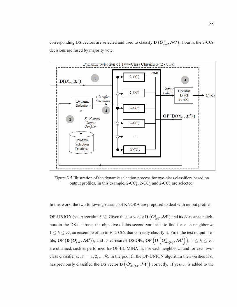
88

corresponding DS vectors are selected and used to classify D(Oi

tst, Mi

). Fourth, the 2-CCs

decisions are fused by majority vote.

Figure 3.5 Illustration of the dynamic selection process for two-class classifiers based onoutput profiles. In this example, 2-CCi

1, 2-CCi3 and 2-CCi

n are selected.

In this work, the two following variants of KNORA are proposed to deal with output profiles.

OP-UNION (see Algorithm 3.3). Given the test vectorD(Oi

tst, Mi

)and its K-nearest neigh-

bors in the DS database, the objective of this second variant is to find for each neighbor k,

1 ≤ k ≤ K, an ensemble of up to K 2-CCs that correctly classify it. First, the test output pro-

file, OP(D

(Oi

tst, Mi

)), and its K-nearest DS-OPs, OP

(D

(Oi

ds(k), Mi

)), 1 ≤ k ≤ K,

are obtained, such as performed for OP-ELIMINATE. For each neighbor k, and for each two-

class classifier cr, r = 1, 2, ...,R, in the pool C, the OP-UNION algorithm then verifies if cr

has previously classified the DS vector D(Oi

ds(k), Mi

)correctly. If yes, cr is added to the

89

ensemble Ek; otherwise, the next 2-CC in the pool is verified. After applying this procedure

to all K-nearest neighbors, the 2-CCs in each ensemble Ek are combined in order to classify

the test vector D(Oi

tst, Mi

). Finally, the final classification label L is obtained by using the

majority vote rule. Note that a same 2-CC can give more than one vote if it correctly classifies

more than one DS vectors.

Inputs:– the number of nearest neighbors, K– the input vector, D

(Oi

tst, Mi)

– the number of random subspaces, R– the pool of 2-CCs, C– the DS output profiles, OP

(D

(Oi

ds(j), Mi))

, 1 ≤ j ≤ M , previously calculated with Algorithm 3.2Outputs:– the final classification label, L1: STEP 1:2: use Algorithm 3.2 to obtain OP

(D

(Oi

tst, Mi))

, where the input vector is D(Oi

tst, Mi)

3: STEP 2:4: find its K nearest output profiles by calculating the Euclidean distance betweenOP

(D

(Oi

tst, Mi))

andeach OP

(D

(Oi

ds(j), Mi))

, where 1 ≤ j ≤ M

5: STEP 3:6: for each neighbor k, 1 ≤ k ≤ K , do7: set count = 1; // number of 2-CCs added to the ensemble8: for each 2-CC cr, r = 1, 2, ...,R, in C do9: if 2-CC cr has previously classified D

(Oi

ds(k), Mi)

correctly and count ≤ K then10: store cr in the ensemble Ek, that is, Ek(count) = cr

11: increment the variable count;12: end if13: end for14: end for15: STEP 4:16: use all Ek, 1 ≤ k ≤ K , to classify D

(Oi

tst, Mi)

17: return the final classification label L by majority voting

Algorithm 3.3 OP-UNION Algorithm.

OP-ELIMINATE (see Algorithm 3.4). Given the test vector D(Oi

tst, Mi

), the objective this

first variant is to find an ensemble of up to K 2-CCs that simultaneously classify its K-nearest

neighbors in the DS database correctly. First, the test output profile, OP(D

(Oi

tst, Mi

)), is

calculated. Its K-nearest DS-OPs, OP(D

(Oi

ds(k), Mi

)), 1 ≤ k ≤ K, are then obtained by

using the Euclidean distance. For each two-class classifier cr, r = 1, 2, ...,R, in the pool C, the

OP-ELIMINATE algorithm verifies if cr has previously classified all corresponding DS vectors

90

D(Oi

ds(k), Mi)

, 1 ≤ k ≤ K, correctly. If yes, cr is added to the ensemble E; otherwise,

the next 2-CC in the pool is verified. In the case where no classifier ensemble can correctly

classify all K DS vectors, the value of K is decreased until at least one 2-CC can correctly

classify one DS vector. Finally, each 2-CC in the ensemble E submites a vote on the test

vector D(Oi

tst, Mi

), where final classification label L is obtained by using the majority vote

rule.

Inputs:– the number of nearest neighbors, K– the input vector, D

(Oi

tst, Mi)

– the number of random subspaces, R– the pool of 2-CCs, C– the DS output profiles, OP

(D

(Oi

ds(j), Mi))

, 1 ≤ j ≤ M , previously calculated with Algorithm 3.2Outputs:– the final classification label, L1: STEP 1:2: use Algorithm 3.2 to obtain OP

(D

(Oi

tst, Mi))

, where the input vector is D(Oi

tst, Mi)

3: STEP 2:4: find its K nearest output profiles by calculating the Euclidean distance betweenOP

(D

(Oi

tst, Mi))

andeach OP

(D

(Oi

ds(j), Mi))

, where 1 ≤ j ≤ M

5: STEP 3:6: set count = 1; // number of 2-CCs added to the ensemble7: for each 2-CC cr, r = 1, 2, ...,R, in C do8: if 2-CC cr has previously classified all D

(Oi

ds(k), Mi)

, 1 ≤ k ≤ K , correctly and count ≤ K then9: store cr in the ensemble E, that is, E(count) = cr;

10: increment the variable count;11: end if12: end for13: STEP 4:14: if size(E) == 0 then15: decrement K16: repeat the process from STEP 317: end if18: STEP 5:19: use the 2-CCs in E to classify D

(Oi

tst, Mi)

20: by majority voting, return the final classification label L

Algorithm 3.4 OP-ELIMINATE Algorithm.

91

3.2.5 Complexity Analysis

The following complexity analysis considers the use of the Forward-Backward algorithm (Ra-

biner, 1989) for HMMs employed in the generative stage, and Support Vector Machines (SVM)

with Radial Basis Function (RBF) kernel (Burges, 1998) in the discriminative stage. Assume a

left-to-right HMM with S states, in which only transitions between two consecutive states are

allowed, and a sequence of lenght L. The Forward-Backward algorithm has a complexity of

O(LS) per iteration, in terms of both time and memory (Alpaydin, 2004; Khreich et al., 2010).

For the SVM-RBF, the time and memory complexity during training is O(DN2), where N is

the size of the training set and D is the number of input dimensions. During operations, the

evaluation of each input sample has a time and memory complexity of O(DV ), where V is the

number of support vectors (Burges, 1998; Cao et al., 2008).

Table 3.1 presents the overall time complexities associated with the generative and discrimina-

tive stages, where the proposed SV system is composed of a bank of B HMMs and a pool of R

SVMs, respectively. In the discriminative stage, α genuine samples vs. β forgery samples are

used to train the SVMs (i.e., N = α + β), while only α genuine samples are used to train each

HMM in the generative stage. The DS strategies proposed in this paper are applied only during

operations, where K is the number of nearest output profiles. Note that the output profiles are

obtained from the pool of SVMs, whose complexity is shown in the second column.

Table 3.1 Time complexities of the generative and discriminative stages

Phase Bank of HMMs Pool of SVMs OP-ELIM./UNIONTraining O(αBLS) O(RDN2) -

Test O(BLS) O(RDV ) O(KR)

92

3.3 Experimental Methodology

Given the generative-discriminative system proposed in Section 3.2, two scenarios are investi-

gated:

1) Scenario 1 – abundant data. A considerable number of genuine signatures per writer

(i.e., 30) is assumed to be available to design an off-line SV system. The objective of this

scenario is to analyse the impact of using the proposed DS strategies over other relevant

ensemble selection strategies found in the literature.

2) Scenario 2 – sparse data A limited number of genuine signatures per writer is assumed to

be available to design an off-line SV system. The objective of this scenario is to apply the

proposed system to two realistic cases of SV. In the first case, three different systems are

designed, each one with 4, 8 and 12 genuine signatures per writer. In the second case, a

system is initially designed with 4 genuine signatures per writer, and new genuine samples

available overtime are incrementaly added to system, without retraining the actual classi-

fiers.

The rest of this section describes the signature databases, the grid segmentation scheme, the

classifier training specifications and the performance evaluation method used in the experi-

ments.

3.3.1 Off-line SV Databases

Two different off-line signature databases are used for proof-of-concept computer simulations:

the Brazilian SV database from PUCPR, used by our research group (Batista et al., 2010a;

Justino et al., 2000; Bertolini et al., 2010; Batista et al., 2010b), and the GPDS database (Var-

gas et al., 2007), used by other researchers (Ferrer et al., 2005; Martinez et al., 2004; Pirlo

et al., 2009; Vargas et al., 2011). While the Brazilian SV database is composed of random,

simple and skilled forgeries, the GPDS database is composed of random and skilled forgeries.

93

3.3.1.1 Brazilian SV database

As presented in Chapter 2, the Brazilian SV database contains 7920 samples of signatures

that were digitized as 8-bit greyscale images over 400X1000 pixels, at resolution of 300 dpi.

The signatures were provided by 168 writers and are organized in two sets: the development

database (DBdev) and the exploitation database (DBexp).

DBdev contains signature samples from writers not enrolled to the system, and is used as prior

knowledge to design the codebooks and the impostor class. It is composed of 4320 genuine

samples supplied by 108 writers. Each writer j has 40 genuine samples, where 20 are available

for training (T j

dev(20)) and 10 for validation (Vj

dev(10)). The remaining 10 samples, available for

test, are not employed in this work.

DBexp contains signature samples from writers enrolled to the system, and is used to model

the genuine class. It is composed of 3600 signatures supplied by 60 writers. Each writer has

40 genuine samples, 10 simple forgeries and 10 skilled forgeries. In the first scenario, 20

genuine samples are available for training (T iexp(20)) and 10 for validation (V i

exp(10)). In the sec-

ond scenario, 4, 8 and 12 genuine samples are available for training, taken from T iexp(20). The

test set is the same for Scenarios 1 and 2, that is, each writer in DBexp has 10 genuine sam-

ples (TST itrue(10)), 10 random (TST i

rand(10)) forgeries, 10 simple (TST isimp(10)) forgeries and

10 skilled forgeries (TST iskil(10)); where the random forgeries are genuine samples randomly

selected from other writers in DBexp.

Given a writer i enrolled to the system, DBdev and DBexp are used to compose different

datasets employed in different phases of the system design (see Table 3.2).

3.3.1.2 GPDS database

The GPDS database is composed of 16200 signature images digitized as 8-bit greyscale at

resolution of 300 dpi. It contains 300 writers, where the first 160 are set as DBexp and the

remaining 140, as DBdev. For each writer in both DBexp and DBdev, there are 24 genuine

94

Table 3.2 Datasets for a specific writer i, using the Brazilian SV database

(a) Scenario 1 – designDataset Name Task Genuine Samples Random Forgery Samples

DBihmm HMM Training T i

exp(20) + V iexp(10) T j=1:108

dev(20) + Vj=1:108dev(10)

DBisvm SVM Training T i

exp(20) 20 from T j=1:108dev(20)

DBigrid SVM Grid Search

V iexp(10)

10 from Vj=1:108dev(10)

DBiroc ROC Curve

Vj=1:108dev(10)

DBids Dynamic Selection

(b) Scenario 2 – designDataset Name Task Genuine Samples Random Forgery Samples

DBihmm HMM Training

4, 8, 12 from T iexp(20)

4x108, 8x108, 12x108from T j=1:108

dev(20)

DBisvm SVM Training 4, 8, 12 from T j=1:108

dev(20)

DBigrid SVM Grid Search 4, 8, 12 from Vj=1:108

dev(10)

DBiroc ROC Curve

Vj=1:108dev(10)

DBids Dynamic Selection

(c) Scenarios 1 and 2 – operationsDataset Name Genuine Samples Forgery Samples

DBitst

TST itrue(10) TST i

rand(10) + TST isimp(10) + TST i

skil(10)

signatures and 30 skilled forgeries. In the literature, only 80 to 160 writers (out of 300) are

used to develop the SV systems, which allow us to work with two datasets.

As this database has a limited number of genuine signatures per writer, it is employed only in

Scenario 2 (see Table 3.3). For each writer j in DBdev, 14 genuine signatures are available

for training (T j

dev(14)) and 10 for validation (Vj

dev(10)); while in DBexp, each writer i has 14

genuine signatures available for training (T idev(14)) and 10 for test (TST i

true(10)). Moreover, 10

random forgeries (TST irand(10)) and 10 skilled forgeries (TST i

skil(10)) are used for test, where

the random forgeries are genuine samples randomly selected from other writers in DBexp.

95

During the comparative analysis performed with systems in the literature (presented in Section

3.4.4), 30 skilled forgeries (TST iskil(30)) are used for test, instead of 10.

In the following sections, the GPDS database is refered as GPDS-160, since a set of 160 writers

(that is, DBexp) is actually modeled by the proposed system.

Table 3.3 Datasets for a specific writer i, using the GPDS database

(a) Scenario 2 – designDataset Name Task Genuine Samples Random Forgery Samples

DBihmm HMM Training

4, 8, 12 from T iexp(14)

4x140, 8x140, 12x140from T j=1:140

dev(14)

DBisvm SVM Training 4, 8, 12 from T j=1:140

dev(14)

DBigrid SVM Grid Search 4, 8, 12 from Vj=1:140

dev(10)

DBiroc ROC Curve

Vj=1:140dev(10)

DBids Dynamic Selection

(b) Scenario 2 – operationsDataset Name Genuine Samples Forgery Samples

DBitst TST i

true(10)

TST irand(10)+TST i

skil(10)

TST irand(10) + TST i

skil(30)

3.3.2 Grid Segmentation

For the Brazilian SV database, the signature images (composed of 400x1000 pixels) are divided

in 62 horizontal cells, where each cell is a rectangle composed of 40x16 pixels. This grid size

along with density of pixels have been successfully applied to this database in (Justino et al.,

2000).

A similar grid segmentation scheme is applied to the GPDS-300 database, even if no previous

work have been done in order to find the best cell size. Although this database contains images

96

of different sizes (that vary from 51x82 pixels to 402x649 pixels), they are represented in a

grid of 400x650 pixels, and segmented in 65 horizontal cells of 40x10 pixels.

To absorb the horizontal variability of the signatures, the images are aligned to the left and the

blank cells in the end of the images are discarded. Therefore, the images may have a variable

number of horizontal cells, while the number of vertical cells is always 10, as shows the exem-

ple of Figure 3.6.

Figure 3.6 Example of grid segmentation scheme.

3.3.3 Training of the Generative Stage

29 different codebooks q (1 ≤ q ≤ 29) are generated by varying the number of clusters from 10

to 150, in steps of 5; using all training and validation signatures of DBdev. In Scenario 1, given

a writer i and a codebook q, 20 genuine samples are taken from DBihmm (i.e., T i

exp(20)) and used

to train a set of discrete left-to-right HMMs with different number of states. As the number

of states varies from 2 to the lenght of the smallest sequence used for training (Lmin), the

genuine space, w1, is composed of a variable number HMMs (i.e., 29x(Lmin-1)) that depends

on the writer’s signature size. On the other hand, to compose the impostor space, w2, there

97

are thousands of HMMs taken from the writers in DBdev (each writer j in DBdev has a set of

HMMs trained with his/her genuine samples).

As performed in Chapter 2, each HMM is trained by using the Baum-Welch Forward-Backward

algoritm (Rabiner, 1989), and at each iteration t, the error Et is calculated (see Equation 2.5).

The goal is to reach an error of 10−5 or smaller (Justino, 2001). Besides this stop criteria, a

validation set (i.e., V iexp(10), available only for Scenario 1) is used in order to select the optimal

training point before overfitting.

In Scenario 2, the number of training sequences is dramatically reduced to 4, 8 and 12. For a

given training sequence Oiq, a set of HMMs is trained by varying the number of states from 2

to 13

of the sequence’s size. The use of a single training sequence per HMM was previoulsy

investigated in (Bicego et al., 2004). The main advantage of this strategy is that it allows to

obtain a higher number of HMMs, adding more diversity to the next system stage.

3.3.4 Training of the Discriminative Stage

Although any discriminative two-class classifier can be used in the second stage, the SVM

classifier with RBF kernel (Chang and Lin, 2001) was chosen because of its successful use in

different pattern recognition problems.

By employing the LIBSVM toolbox (Chang and Lin, 2001), the parameters C and È are found

through a gridsearch technique. For each different pair {C, È}, 10 different SVMs are trained

using a variant of the cross-validation method, where the genuine samples performs the usual

rotation, and the random forgery samples are changed each time. Since the number of genuine

samples in DBigrid can be smaller than the number of SVMs to be trained (i.e., in Scenario

2), the same genuine samples are used to train more than one SVM. On the other hand, new

random forgery samples are selected, randomly and with remplacement, each time that a new

SVM training is performed. Finally, the error rates provided by the 10 SVMs are averaged, and

the pair {C, È} providing the smallest error rates are used to train the final SVMs.

98

By using the specialized RSM (see Algorithm 3.1) with R′ = S ′ = 15, 100 SVMs are trained

per writer. Note that, for a same writer i, the training set, DBisvm, remains the same for all 100

SVMs.

3.3.5 Classifier Ensemble Selection

In this work, the simulation results obtained with OP-UNION and OP-ELIMINATE are com-

pared with KNORA-UNION/ELIMINATE (Ko et al., 2008), the standard combination of all

classifiers, and Decision Templates (DT) (Kuncheva et al., 2001).

With OP-UNION and OP-ELIMINATE, the search for the K-nearest neighbors is done by

using the output labels provided by all 100 SVMs; while with KNORA-UNION and KNORA-

ELIMINATE, only the SVM input subspace providing the lowest error rates on DBids is used

during the search. The value of K is defined as being half of the number of genuine samples

in DBids. If the value of K is even, K + 1 classifiers are used in order to avoid votes that result

in a tie. In Scenario 1, K is set as 5; while in Scenario 2, K is set as 3, 5 and 7.

The standard combination of classifiers consists of sending the test vector D(Oi

tst, Mi

)to all

100 SVMs and then fusing their corresponding output labels by majory vote. If a tie vote is

obtained, the final output label is randomly chosen.

The decision templates (DTs) is a well-known DS method in the multi-classifier system (MCS)

community (Kuncheva et al., 2001). First, each DS vector D(Oi

ds(j), Mi)

, 1 ≤ j ≤ M , is

sent to all SVMs, and its corresponding output labels are organized in a decision profile (DP)

matrix, where each line corresponds to a different SVM and each column corresponds to a

different class. Since we work with 100 two-class SVMs, each DP(D

(Oi

ds(j), Mi))

is

composed of 2 columns and 100 lines, where each cell contains the value 1 or 0. For instance,

if the 100th SVM classifies D(Oi

ds(j), Mi)

as belonging to the genuine class C1, the cell

located in line 100 and column 1 will contain the value 1, while the cell located in line 100

and column 2 (which corresponds to the class C2) will contain the value 0. Then, a decision

99

template (DT) is calculated for each class Cj (j = 1, 2) by averaging the DPs of the DS vectors

belonging to this class. When a test vector D(Oi

tst, Mi

)is presented, its decision profile

matrix DP(D

(Oi

tst, Mi

))is calculated and compared to the decision templates DT(Cj).

The comparison is done by using the Euclidean distance, and the higher the similarity between

DP(D

(Oi

ds(j), Mi

))and DT(Cj), the higher the support for class Cj. Finally, the most

likely DT(Cj) is selected and the output label the most represented in this template is assigned

to D(Oi

ds(j), Mi

).

The DS strategies proposed in this paper are compared as well with two reference systems pro-

posed in our previous work, that is, (i) a traditional generative system based on HMMs (Batista

et al., 2010a) (refered in this paper as baseline system), and (ii) a hybrid system based on the

static selection of generative-discriminative ensembles (Batista et al., 2010b). Both systems

are briefly described in Section 3.4.1.

3.3.6 Performance Evaluation

The system performance is measured by an averaged ROC curve generated using DBiroc, ac-

cording to the method of Jain and Ross (2002). As explained in Chapter 2, the operating points

associated with a same γ value (and related to different users) are averaged. Recall that γ corre-

sponds to the true negative rate (TNR) and that it may be associated with different thresholds.

Since different 2-CCs are trained through the Random Subspace Method, each 2-CC results in

a different averaged ROC curve.

During operations, FNR and FPR are calculated regarding different γ values of the averaged

ROC curves. The average error rate (AER), also computed for different γ values, indicates the

total error of the system, where FNR and FPR are averaged taking into account the a priori

probabilities. When the Brazilian SV database is used, the FPR is calculated with respect

to three forgery types: random, simple and skilled (see DBitst of Table 3.2); while for GPDS

database, FPR is calculated with respect to random and skilled forgeries (see DBitst of Table

100

3.3).

3.4 Simulation Results and Discussions

3.4.1 Reference Systems

In Chapter 2, a baseline off-line SV system was designed under a traditional HMM-based

approach, which consists of training a single HMM per writer (see also ref. Batista et al.

(2010a)). By using DBihmm (see Table 3.2 (a)) and a single codebook, multiple HMMs were

trained with a different number of states in order to isolate an HMM order that provides the

smallest error Et (see Equation 2.5). This resulted in an AER (γ = 1.0) of 8.50% on test data.

To reduce error rates and exploit the sub-optimal HMMs discarded by this baseline system,

a multi-hypothesis system was also designed. By training a set of HMMs with a different

number of states, and then selecting the most accurate HMM for each operating point of the

ROC space, an AER (γ = 1.0) of 7.79% was obtained on test data.

In another work, a hybrid system based on the static selection of generative-discriminative en-

sembles was proposed (see also ref. Batista et al. (2010b) and Appendix I). Given the same

HMMs generated through the multi-hypothesis approach, only the most representative HMMs

were selected to compose the generative stage, by using a greedy search algorithm. The rep-

resentative HMMs were then employed as a feature extractors for the discriminative stage. To

generate a pool of SVMs, a different SVM was trained using DBisvm (see Table 3.2 (a)), each

time that the greedy algorithm added a new representative HMM to the system. Then, the ICON

algorithm (Ulas et al., 2009) was applied in order to incrementally construct the ensemble. Like

the model selection algorithm, ICON consists in a greedy process that, during each iteration,

chooses the SVM that most improves system performance on validation data when added to the

ensemble. A margin-based measure called CI (from Chebishev’s inequality) (Breiman, 2001;

Kapp et al., 2007) was employed to assess the performance of each ensemble. This resulted in

an AER (γ = 1.0) of 5.50% on test data – which represents an improvement of 2.50% with

101

respect to the baseline system of Chapter 2. Figure 3.8 shows the corresponding AERs curves.

3.4.2 Scenario 1 – abundant data

In this experiment, each DBids is composed of 10 genuine samples supplied by writer i (in

DBexp) versus 1080 random forgery samples taken from writers not enrolled to the system

(see Table 3.2 (a)). Note that the random forgery samples are the same for all writers in DBexp.

Figure 3.7 shows the averaged ROC curves obtained with scores produced from 100 different

SVMs using DBiroc , while Figure 3.8 presents the AERs curves on test data (DBi

tst), as

function of operating points (γ).

0 0.05 0.1 0.15 0.2 0.25 0.3 0.35 0.4 0.45 0.50.91

0.92

0.93

0.94

0.95

0.96

0.97

0.98

0.99

1

FPR

TP

R

Figure 3.7 Averaged ROC curves obtained with scores produced from 100 differentSVMs using DBi

roc (from Brazilian data), under Scenario 1.

Results indicate that OP-ELIMINATE and OP-UNION strategies provided the lowest AERs,

demonstrating the advantage of using a DS approach based on output profiles – as opposed to

102

KNORA, where the input feature space is used to find the K-nearest DS samples. It is also

beneficial to employ EoCs composed of a small set of base classifiers – in contrast to Decision

Templates and to the standard combination of classifiers, where all base classifiers in the pool

are part of the ensemble.

OP-ELIMINATE and OP-UNION also achieved AERs that are lower than those obtained with

SS, showing that the proposed DS strategies are more suitable for SV, where a significant level

of uncertainty resides due to the availability of partial knowledge during system design. Gen-

eraly, only genuine and random forgery samples are available to design a SV system. This

system, in turn, must detect other forgery types during operations. Finally, the fewer perfor-

mance of the baseline system is obtained because a pure generative approach was adopted for

system design, where only the genuine class is modeled. Tables 3.4 and 3.5 present the overall

results for γ = 0.90 and γ = 1.0, respectively.

0 0.86 0.88 0.90 0.92 0.94 0.96 0.98 15

10

15

20

25

30

35

Operating Points (γ)

AER

(%)

OP−UNIONOP−ELIMINATEKNORA−UNIONKNORA−ELIMINATEDecision TemplatesCombination of 100 SVMsBaseline SystemStatic Selection

Figure 3.8 AERs versus operating points (γ) obtained on Brazilian test data withdifferent SV systems, under Scenario 1.

103

Table 3.4 Overall error rates (%) obtained on Brazilian test data for γ = 0.90, underScenario 1

Method FNR FPRrandom FPRsimple FPRskilled AEROP-UNION 3.33 1.67 3.83 34.83 10.92

OP-ELIMINATE 4.67 1.33 2.83 30.00 9.71KNORA-UNION 2.17 2.50 7.00 45.33 14.25

KNORA-ELIMINATE 2.33 2.67 6.33 44.33 13.92Decision Templates 2.17 2.17 7.17 45.50 14.25

Combination of 100 SVMs 2.00 2.67 8.17 47.33 15.04Static Selection (Batista et al., 2010b) 2.17 8.00 5.83 35.17 12.79

Baseline (Batista et al., 2010a) 0.33 12.17 20.67 78.83 28.00

Table 3.5 Overall error rates (%) obtained on Brazilian test data for γ = 1.0, underScenario 1

Method FNR FPRrandom FPRsimple FPRskilled AEROP-UNION 8.17 0.67 0.67 14.00 5.88

OP-ELIMINATE 7.50 0.33 0.50 13.50 5.46KNORA-UNION 8.17 0.67 0.67 14.67 6.04

KNORA-ELIMINATE 7.83 0.67 0.67 14.17 5.83Decision Templates 8.67 0.50 0.67 15.17 6.25

Combination of 100 SVMs 8.83 0.50 0.67 15.33 6.33Static Selection (Batista et al., 2010b) 13.50 0.00 0.17 8.33 5.50

Baseline (Batista et al., 2010a) 12.67 0.33 1.17 19.83 8.50

3.4.3 Scenario 2 – sparse data

In this experiment, each DBids is composed of 4, 8 and 12 genuine samples supplied by writer

i (in DBexp) versus several random forgery samples taken from writers not enrolled to the

system (see Tables 3.2 (b) and 3.3 (a)), where the random forgery samples are the same for

all writers in DBexp. Figure 3.9 presents a comparison between the baseline system (Batista

et al., 2010b) and OP-ELIMINATE, when trained with 4, 8 and 12 genuine samples from the

Brazilian SV database. The results obtained by these systems when trained with 20 genuine

samples, previously presented in Scenario 1, are also shown in this graph. As expected, system

performance improves as more genuine samples are used for training. Such an improvement

104

is less pronounced with the baseline system. As with Scenario 1, the proposed system reached

the smallest AERs.

0 0.86 0.88 0.90 0.92 0.94 0.96 0.98 15

10

15

20

25

30

35

Operating Points (γ)

AE

R (%

)

Baseline (#trn = 4)Baseline (#trn = 8)Baseline (#trn = 12)Baseline (#trn = 20)OP−ELIM. (#trn = 4)OP−ELIM. (#trn = 8)OP−ELIM. (#trn = 12)OP−ELIM. (#trn = 20)Static Sel. (#trn = 20)

Figure 3.9 AERs versus operating points (γ) obtained on Brazilian test data with thebaseline system and OP-ELIMINATE, under Scenario 2.

Figures 3.10 and 3.11 show the AERs obtained with the proposed systems for both Brazilian

and GPDS-160 databases, and Table 3.6 presents the overall error rates obtained for γ = 0.9;

where #trn indicates the number of genuine signatures in the training set (i.e., DBihmm and

DBisvm), and #ds indicates the number of genuine signatures in DBi

ds. Note that Table 3.6 (d)

is related to the Scenario 1, where the training and DS sets differ. See Appendix II for error

rates related to other operating points (γ).

The proposed system achieved higher error rates with the GPDS-160 database because it con-

tains different image sizes, which vary (vertically and horizontally) even for a same writer. In

this work, no normalization technique was employed. As explained in Section 3.3.2, a fixed-

sized grid – suitable for the Brazilian SV database – was applied to the GPDS-160 database.

105

With the Brazilian SV database, the region used for signing does not vary, since it simulates

the case where the signature samples come from a same type of document, i.e., checks from a

specific bank.

OP-UNION seems to be more suitable than OP-ELIMINATE when the base classifiers are

trained with a very small number of signatures (for instance, 4 genuine signatures vs. 4 random

forgeries). In fact, since classifiers trained with few signature samples are not very accurate, it

is desirable to select a higher number of classifiers to form an EoC.

0 0.86 0.88 0.90 0.92 0.94 0.96 0.98 15

10

15

20

25

30

35

Operating Points (γ)

AE

R (%

)

GPDS−160 (#trn = 4)GPDS−160 (#trn = 8)GPDS−160 (#trn = 12)Brazilian (#trn = 4)Brazilian (#trn = 8)Brazilian (#trn = 12)

Figure 3.10 AERs versus operating points (γ) obtained on Brazilian and GPDS-160 testdata with OP-ELIMINATE strategy, under Scenario 2.

The final experiment investigates the adaptive capabilities of the proposed system when new

genuine signatures are integrated incrementally. A limited number of genuine signatures are

used to design both generative and discriminative stages. Then, the goal is to gradually improve

system performance by adding new genuine signatures to DBids.

106

0 0.86 0.88 0.90 0.92 0.94 0.96 0.98 15

10

15

20

25

30

35

Operating Points (γ)

AE

R (%

)

GPDS−160 (#trn = 4)GPDS−160 (#trn = 8)GPDS−160 (#trn = 12)Brazilian (#trn = 4)Brazilian (#trn = 8)Brazilian (#trn = 12)

Figure 3.11 AERs versus operating points (γ) obtained on Brazilian and GPDS-160 testdata with OP-UNION strategy, under Scenario 2.

First, DBids is composed of 4 genuine signatures versus 1080 random forgeries from DBdev,

as performed in the previous experiment. Then, DBids is updated twice, by adding 4 new

genuine signatures each time. Figures 3.12 and 3.13 show the AER curves (in bold) obtained

with OP-ELIMINATE using the Brazilian and GPDS-160 databases, respectively. The AER

curves related to the systems trained with 8 genuine samples and 12 genuine samples, from the

previous experiment, are also presented in these figures.

The addition of newly-obtained genuine samples in DBids improved system performance in

almost all operating points. With the Brazilian SV database (see Figure 3.12), the performance

of the system using 4 genuine samples for training and 8 for DS is comparable to that of using

8 genuine samples for both training and DS in some operating points, such as γ = 0.91 and

γ = 0.87. With the GPDS-160 database (see Figure 3.13), the performance of the system using

4 signatures for training and 12 for DS is comparable to or better than that of using 12 genuine

samples for both training and DS, when γ ≤ 0.92.

107

Table 3.6 Overall error rates (%) obtained on Brazilian and GPDS-160 test data forγ = 0.90, under Scenario 2.

(a) #trn = 4, #ds = 4, K = 3

Database Method FNR FPRrandom FPRsimple FPRskilled AER

BrazilianBaseline 16.17 9.67 15.00 67.83 27.17

OP-UNION 26.17 10.83 9.33 35.17 20.38OP-ELIMINATE 27.33 11.67 10.50 34.83 21.08

GPDS-160 OP-UNION 19.44 12.62 N/A 48.69 26.92OP-ELIMINATE 20.69 16.56 N/A 50.50 29.25

(b) #trn = 8, #ds = 8, K = 5

Database Method FNR FPRrandom FPRsimple FPRskilled AER

BrazilianBaseline 8.00 11.00 19.17 73.33 27.87

OP-UNION 11.33 11.83 9.67 42.33 18.79OP-ELIMINATE 16.00 11.33 8.67 38.83 18.71

GPDS-160 OP-UNION 14.88 11.44 N/A 49.00 25.10OP-ELIMINATE 16.62 11.62 N/A 48.75 25.67

(c) #trn = 12, #ds = 12, K = 7

Database Method FNR FPRrandom FPRsimple FPRskilled AER

BrazilianBaseline 5.17 11.50 19.33 73.83 27.46

OP-UNION 7.83 10.67 10.50 43.33 18.08OP-ELIMINATE 13.50 5.67 6.83 34.33 15.08

GPDS-160 OP-UNION 13.75 11.62 N/A 53.94 26.44OP-ELIMINATE 19.19 9.81 N/A 47.25 25.42

(d) #trn = 20, #ds = 10, K = 5 (from Scenario 1)Database Method FNR FPRrandom FPRsimple FPRskilled AER

Brazilian

Baseline 0.33 12.17 20.67 78.83 28.00Static Selection 2.17 8.00 5.83 35.17 12.79

OP-UNION 3.33 1.67 3.83 34.83 10.92OP-ELIMINATE 4.67 1.33 2.83 30.00 9.71

The main advantage of adapting DBids incrementally is that the actual classifiers need not

be retrained. Moreover, more genuine signatures may be exploited by OP-UNION and OP-

ELIMINATE during the dynamic selection of classifiers. Although more complexes, the sys-

tems trained with 8 and 12 genuine samples provide, in general, lower error rates compared to

the system trained with 4 genuine samples and using 8 and 12 samples for DS, respectively.

Therefore, incremental updating of DBids represents a viable measure to improve system per-

formance, and may be used in conjuction with incremental learning (IL) of classifiers.

108

0 0.86 0.88 0.90 0.92 0.94 0.96 0.98 112

14

16

18

20

22

24

Operating Points (γ)

AE

R (%

)

#trn = 4 (#ds = 4 )#trn = 8 (#ds = 8 )#trn = 12 (#ds =12)#trn = 4 (#ds = 8 )#trn = 4 (#ds =12)

Figure 3.12 AERs versus operating points (γ) obtained on Brazilian test data withincremental updating and OP-ELIMINATE strategy, under Scenario 2.

3.4.4 Comparisons with systems in the literature

Table 3.7 presents the error rates provided by systems designed with the Brazilian SV database.

While Bertolini et al. (2010) and Santos et al. (2004) proposed discriminative systems based

on dissimilarity representation, Justino et al. (2001) proposed a traditional generative system

based on HMMs. Finally, Batista et al. (2010a) proposed a multi-hypothesis system based on

HMMs (note that it represents the same system of Chapter 2). Since these systems required

a considerable number of signatures for training, they are compared with the best system ob-

tained in Scenario 1.

Comparisons with other systems is difficult because of the use of different features, databases

and experimentation protocols. In our research, only genuine signatures and random forgeries

are considered during training, validation and thresholding, since other forgery types are not

available during the design of a real-world SV system. However, some authors have used

109

0 0.86 0.88 0.90 0.92 0.94 0.96 0.98 121

22

23

24

25

26

27

28

29

30

31

Operating Points (γ)

AE

R (%

)

#trn = 4 (#vld = 4 )#trn = 8 (#vld = 8 )#trn = 12 (#vld =12)#trn = 4 (#vld = 8 )#trn = 4 (#vld =12)

Figure 3.13 AERs versus operating points (γ) obtained on GPDS test data withincremental updating of DBi

ds and OP-ELIMINATE strategy, under Scenario 2.

Table 3.7 Overall error rates (%) provided by systems designed with the Brazilian SVdatabase

Reference FNR FPRrandom FPRsimple FPRskilled AERBatista et al. (2010a) 9.83 0.00 1.00 20.33 7.79Bertolini et al. (2010) 11.32 4.32 3.00 6.48 6.28Justino et al. (2001) 2.17 1.23 3.17 36.57 7.87Santos et al. (2004) 10.33 4.41 1.67 15.67 8.02

OP-ELIMINATE (γ = 1.0) 7.50 0.33 0.50 13.50 5.46

skilled forgeries to select optimal decision thresholds. In order to compare with systems that

use the GPDS database, the equal error rate (EER) – obtained when the threshold is set to have

the FNR approximately equal to the FPR – is employed. Two operating points are chosen

from the test scores: one regarding genuine signatures vs. random forgeries, and a second

regarding genuine signatures vs. skilled forgeries (where 30 skilled forgeries are employed,

instead of 10). Table 3.8 presents the EERs provided by the proposed system and other

110

systems designed with different subsets of the GPDS database. Following the same evaluation

critera, the results obtained with the Brazilian SV database are also shown in Table 3.8.

Table 3.8 EERs (%) provided by the proposed system and by other systems in theliterature

(a) genuine signatures vs. random forgeriesReference Database #trn FNR (%) FPR (%)

Ferrer et al. (2005) GPDS-1604 4.30 3.808 2.50 2.4012 2.20 3.30

Vargas et al. (2011) GPDS-100 5 3.75 3.7510 1.76 1.76

OP-UNION GPDS-1604 7.75 6.568 5.38 5.4412 4.50 5.19

OP-UNION Brazilian4 7.67 8.338 4.17 4.6712 2.83 3.67

(b) genuine signatures vs. skilled forgeriesReference Database #trn FNR (%) FPR (%)

Ferrer et al. (2005) GPDS-1604 17.30 14.908 13.40 14.90

12 14.10 12.60Martinez et al. (2004) GPDS-160 - 9.56 9.56

Pirlo et al. (2009) GPDS-40 - 19.00 21.00

Vargas et al. (2011) PDS-100 5 12.06 12.0610 9.02 9.02

OP-UNION GPDS-1604 20.75 20.318 16.69 17.38

12 16.81 16.88

OP-UNION Brazilian4 19.00 20.178 14.33 14.67

12 12.17 12.67

3.4.5 System Complexity

In Scenario 1, Q(Lmin −1) HMMs are trained per writer, where Q is the number of codebooks

(i.e., 29) and Lmin is the size of the smallest training sequence. On the other hand, αQ(13L−1)

HMMs are trained per writer in Scenario 2, where α is the number of genuine signatures used

for training and L is the size of the training sequence being modeled. This indicates that this

scenario produces about α/3 times more HMMs than the previous one. Nevertheless, the time

111

complexity to train an individual HMM is lower in Scenario 2, since HMMs are trained with

a single observation sequence, and with a smaller number of states. Recall that the number of

HMM states varies from 2 to Lmin in Scenario 1 and from 2 to 13L in Scenario 2. Regarding the

discriminative stage, each SVM has a fixed input feature dimension of 15+15 (i.e., R′ + S ′).

During the experiments, the number of HMM states varied from 2 to 33 in Scenario 1 and

from 2 to 12 in Scenario 2, on average. By considering only the genuine space, w1, 29x(33-1)

HMMs were trained per writer in Scenario 1, and 4x29x(12-1) HMMs were trained per writer

in Scenario 2, when α = 4. Table 3.9 presents the average number of HMMs, states, SVM

inputs and support vectors employed in each scenario. Despite the overproduction of base

classifiers in both generative and discriminative stages, each individual base classifier holds a

very low complexity.

Table 3.9 Average number of HMMs, states, SVM inputs, and support vectors (SVs) ineach scenario

Scenario α HMMs per writer (w1) HMM states SVM inputs (R′ + S′) SVs per SVM1 20 928 2 to 33

15+15

25

24 1276

2 to 127

8 2552 1112 3828 16

3.5 Discussion

In this chapter, the challenge of designing off-line SV systems from a limited amount of gen-

uine signature samples was addressed through the dynamic selection of hybrid generative-

discriminative ensembles. In the generative stage, multiple discrete left-to-right HMMs are

trained using a different number of states and codebook sizes, and employed as feature extrac-

tors for the discriminative stage. In the discriminative stage, HMM likelihoods are measured

for each training signature, and assembled into feature vectors that are used to train a diver-

sified pool of 2-CCs through a specialized RSM. During operations, a DS strategy selects the

most accurate ensemble of 2-CCs to classify a given input signature. Experiments performed

112

with two real-world signature databases (comprised of genuine samples and random, simple

and skilled forgeries) indicate that the proposed DS strategy can significantly reduce the overall

error rates, with respect to other EoCs formed using well-known dynamic and static selection

strategies. Moreover, the performance of the hybrid generative-discriminative system is greater

than or comparable to that of relevant systems found in the literature.

The use of different codebooks and HMM states allows the system to learn each signature

at different levels of perception. The codebooks – as well as the impostor class – are ob-

tained from signatures of an independent database (i.e., DBdev), ensuring that the SV sys-

tem can be designed with a single user (Appendix III investigates the use of DBexp for both

designing codebooks and the SV system, such as performed by most SV systems based on

discrete HMMs). Another important contribution is the proposal of two new DS strategies

(OP-ELIMINATE and OP-UNION), based on KNORA (Ko et al., 2008) and on output pro-

files (OP) (Cavalin et al., 2010), which were shown to be more suitable for off-line SV than

other well-known dynamic and static selection strategies.

A challenging issue in biometrics is to take into account the aging of reference data in long-

lived systems (Pato and Millett, 2010). In this respect, the proposed generative-discriminative

SV system can be adapted such that newly-obtained genuine samples are used to incrementally

improve its performance overtime, without the need of retraining the actual classifiers.

CONCLUSION

This Thesis focused on the challenge of designing accurate and adaptive off-line SV systems,

based on left-to-right HMMs, with a limited and unbalanced amount of data. Instead of trying

to increase the number of training samples or to select the most discriminative features, the

off-line SV approaches proposed in this Thesis take advantage of the potential availability of

a large number of extracted features to overcome the problem of having a limited amount of

training data. In other words, signatures are represented at different levels of perception and

used to produce multiple classifiers that collaborate together in order to reduce error rates.

Besides, an independent signature database, supplied by writers not enrolled to the SV system,

is employed as prior knowledge of the problem to design the codebooks and the impostor class.

Based on the multi-hypotheses principle, a new approach for combining classifiers in the ROC

space is proposed. By training a set of HMMs with different number of states and codebooks

and then selecting the most accurate HMM(s) for each operating point of the ROC space, we

propose a solution to repair concavities of individual ROC curves, while generating a high

quality composite ROC curve. Besides providing a more accurate estimation of system perfor-

mance during training, the operating points of the composite ROC curve significantly reduces

the error rates during operations. Therefore, since ROC concavities are observed, this ap-

proach is suitable to improve system performance. Another advantage of the multi-hypothesis

approach is that it can be used for dynamic selection of the best classification model – that is,

the best codebook, HMM and threshold – according to the risk linked to an input sample. In

banking applications, for instance, the decision to use a specific operating point may be asso-

ciated with the amount of the check. As an example, if a user rarely signs high value checks,

signing for large amounts would require operating points related to low FPRs, as would be

provided by a γ value close to 1. Lower amounts would translate to operating points related to

low FNRs, since the bank and user would not feel comfortable with frequent false rejections.

Still taking advantage of multiple left-to-right HMMs trained with different states and code-

books, a hybrid generative-discriminative classification architecture is proposed. The use of

114

HMMs as feature extractors in the generative stage followed by SVMs as classifiers in the

discriminative stage allows for a better design not only of the genuine class, but also of the

impostor class. Moreover, this approach provides a more robust learning than a traditional

HMM-based approach when a limited amount of training data is available. Despite the over-

production of base classifiers in both generative and discriminative stages, each individual base

classifier holds a very low complexity.

The last contribution of this Thesis is the proposal of two new strategies for the dynamic selec-

tion (DS) of ensemble of classifiers, namely OP-UNION and OP-ELIMINATE. Experiments

performed with the PUCPR and GPDS signature databases indicate that the proposed DS strate-

gies achieve a higher level of performance in off-line SV than other reference DS and static

selection (SS) strategies from literature. This represents a situation where DS is superior to

SS, i.e., in a problem where a significant level of uncertainty resides due to the availability

of partial knowledge during system design. Finally, OP-UNION and OP-ELIMINATE allow

for the SV system to be adapted such that new genuine signature samples may be integrated

incrementally. As new genuine signature samples become available, the system performance

may be improved overtime, without the need of retraining the actual classifiers.

Although the proposed approaches were validated for the specific problem of off-line SV, they

can be easly adapted to any similar two-class problem, e.g., other applications in biometrics.

Regardless the biometric trait, applications in biometrics generally suffer from the problem of

having a limited number of genuine samples to train a classifier. With respect to the choice

of classifiers, the multi-hypothesis approach can be employed with any generative or discrim-

inative classifier, with the condition that it is possible to generate ROC curves from its out-

puts. Similarly, other generative and discriminative classifiers can be investigated in the hybrid

generative-discriminative architecture, such as, Gaussian Mixture Models (GMMs) followed

by Multi-Layer Perceptrons (MLPs).

115

Future work

Due to time constraints, some interesting issues were not investigated in this Thesis. Therefore,

proposals for future work consist of:

1) Generation of a composite ROC curve for the hybrid generative-discriminative system.

As an alternative to the classifier selection/combination strategies proposed for the hybrid

generative-discriminative system of Chapter 3, the multiple SVMs generated through the

random subspace method could be used to obtain a composite ROC curve (such as pro-

posed in Chapter 2), so that the best SVM(s) would be associated to each operating point of

the curve.

2) Learning of new features incrementally. In Chapter 3, we have shown that each HMM in

the generative stage may be trained by using a single signature sample. In this respect, new

HMMs – and, consequently, new likelihoods – may be added to the system whenever a

new training sample is available. The discriminative stage, however, should be composed

of classifiers able to deal with the addition of new dimensions to the input feature vectors,

such as the K-NN classifier.

3) Investigation of other grid resolutions and features. Although the grid resolution and the

features employed in this Thesis were previously validated by Justino (2001) with the

Brazilian SV database, different grid resolutions/features could be analysed taking into ac-

count other SV databases.

116

LIST OF PUBLICATIONS

Journal Articles

• Batista, L., E. Granger, and R. Sabourin. Dynamic Selection of Generative-Discriminative

Ensembles for Off-Line Signature Verification. Submitted to Pattern Recognition.

• Batista, L., E. Granger, and R. Sabourin. Improving Performance of HMM-based Off-line

Signature Verification Systems through a Multi-Hypothesis Approach. International Journal

on Document Analysis and Recognition (IJDAR), 13:33–47, March 2010.

Conference Articles

• Batista, L., E. Granger, and R. Sabourin. Dynamic Ensemble Selection for Off-Line Sig-

nature Verification. To appear in the Tenth International Workshop on Multiple Classifier

System (MCS’11), Jun 2011.

• Batista, L., E. Granger, and R. Sabourin. Applying Dissimilarity Representation to Off-

Line Signature Verification. In Twentieth International Conference Pattern Recognition

(ICPR’10), pages 1293–1297, August 2010.

• Batista, L., E. Granger, and R. Sabourin. A Multi-Classifier System for Off-line Signature

Verification based on Dissimilarity Representation. In Ninth International Workshop on

Multiple Classifier System (MCS’10), pages 264–273, April 2010.

• Batista, L., E. Granger, and R. Sabourin. A Multi-Hypothesis Approach for Off-line Sig-

nature Verification with HMMs. In International Conference on Document Analysis and

Recognition (ICDAR’09), pages 1315–1319, July 2009.

117

Book Chapter

• Batista, L., D. Rivard, R. Sabourin, E. Granger, and P. Maupin. State of the Art in Off-

line Signature Verification. In B. Verma and M. Blumenstein, editors, Pattern Recognition

Technologies and Applications: Recent Advances. IGI Global, 1st edition, pages 39-62,

2007.

APPENDIX I

STATIC SELECTION OF GENERATIVE-DISCRIMINATIVE ENSEMBLES

The contents of this appendix have been published as a conferece article in (Batista et al.,

2010b). In that work, a hybrid generative-discriminative off-line SV system was proposed,

similar to that of Chapter 3, where the generative stage is composed of HMMs trained by using

a single universal codebook (i.e., CB35) and different number of states, and the discriminative

stage is composed of one or more two-class classifiers, selected through a static strategy.

This system is depicted in Figure AI.1, where only the most representative HMMs, Hi, are

chosen to compose the genuine (w1) and impostor (w2) subspaces for a specific writer i.

Figure AI.1 The hybrid generative-discriminative system, for a specific writer i, usingthree representative HMMs per subspace.

Let Mi = {Φ1 ∪ Φ2}be the bank of available HMMs for a specific writer i, where Φ1is the

set of HMMs trained with genuine samples of writer i, and Φ2is the set of HMMs trained with

119

random forgery samples (i.e., genuine samples from writers not enrolled to the system). By

starting with an empty subspace wn, 1 ≤ n ≤ 2, a greedy algorithm incrementally adds a new

HMM to wn, until a convergence criterion is reached (see Algorithm AI.1).

Basically, a HMM λb is chosen if its addition to the current subspace, wn, minimizes the

AER provided by a 1-NN classifier (with Euclidean distance) on the validation set Oivld(j),

1 ≤ j ≤ M . In other words, when a HMM λb is added to wn, a set of likelihood vectors

D(Oi

vld(j), wn

), 1 ≤ j ≤ M , is obtained such as described in Chapter 3. Then, for each

vector D(Oi

vld(j), wn

), its nearest neighbor is found in the validation set (excluding itself),

and its output label is calculated. After applying this procedure to all validation vectors, the

AER is calculated. If the addition of λb to wn minimizes the AER, it is permanently added

to the bank of representative HMMs, Hi.

Inputs:– the validation set of writer i, composed of genuine samples (class C1) and random forgerysamples (class C2)– the bank of available left-to-right HMMs Mi = {Φn}, 1 ≤ n ≤ 2, where Φn is the set ofHMMs of class nOutputs: the bank of representative HMMs Hi = {wn}, 1 ≤ n ≤ 2

for each class Cn, 1 ≤ n ≤ 2, doset wn← [ ]; //empty subspaceset m ← 0; //number of models stored in wn

repeatm ← m + 1;find the HMM λb in Φn that, when added to wn(m), provides the smallest AER of a1-NN classifier using the validation set;remove λb from the set Φn;

until AER reaches a minimum valueend forstore each subspace wnin Hi, that is, Hi = {wn}, 1 ≤ n ≤ 2;return Hi;

Algorithm AI.1 Selection of representative HMMs for a specific writer i.

The rest of this appendix presents the experiments performed with the hybrid generative-

discriminative system using the Brazilian SV database. Except for the fact that only one

120

codebook is used, the experimentation protocol is similar to that employed in Scenario 1 of

Chapter 3.

Hybrid Generative-Discriminative System vs. Baseline System

Given the bank of available left-to-right HMMs, Mi = {Φ1 ∪ Φ2}, and the validation set of

writer i, Algorithm I.1 was applied to select the most representative HMMs, Hi = {w1∪w2}.

This procedure was repeated for each writer in DBexp, and, on average, 2 HMMs were selected

to compose w1, and 3 HMMs were selected to compose w2. Then, by using Hi and a set of

training sequences Oitrn(l), 1 ≤ l ≤ N , likelihood vectors D

(Oi

trn(l), Hi)

, 1 ≤ l ≤ N were

obtained and used to train a single SVM per writer.

The averaged ROC curve representing the generative-discriminative system (obtained with val-

idation scores) is indicated by the square-dashed line in Figure AI.2. The circle-dashed curve

corresponds to the baseline system, designed under a traditional HMM-based SV approach

(see Chapters 2 and 3). Table AI.1 (a) and (b) present the error rates on test for both systems

regarding different operating points (γ). Note that the proposed system provided a reduction in

the AER from 2.5%, for γ =1, up to 9.87%, for γ = 0.95.

Static Selection of SVMs Ensembles

The next experiment consisted of analyzing the impact of using an ensemble of SVMs per

writer in the discriminative stage, where each SVM of the ensemble is selected through a static

approach. In order to generate a pool, a different SVM is trained each time that a new HMM

is selected by Algorithm I.1. For example, given that w1 is represented by the HMMs {a, b, c}

and w2, by {d, e}, six base SVMs can be produced by using {w1∪w2}, that is, {a, d}; {a, d, e};

{a, b, d}; {a, b, d, e}; {a, b, c, d} and {a, b, c, d, e}.

Once the pool of SVMs is obtained, the algorithm ICON (Ulas et al., 2009) is applied in order

to incrementally construct the ensemble. Such as Algorithm I.1, ICON consists in a greedy

process, at each iteration, chooses the classifier that best improves the system performance (on

validation data) when added to the current ensemble.

121

0 0.02 0.04 0.06 0.08 0.1 0.12 0.14 0.16 0.18 0.20.88

0.9

0.92

0.94

0.96

0.98

1

FPR

TP

R

Proposed SystemBaseline System

0 0.005 0.01 0.015 0.02 0.025 0.03 0.0350.98

0.9825

0.985

0.9875

0.99

0.9925

0.995

0.9975

1

FPR

TP

R

γ = 1

γ = 1

Figure AI.2 Averaged ROC curves of the baseline and proposed systems.

In this work, a measure called CI (from Chebishev’s inequality) (Breiman, 2001; Kapp et al.,

2007) was employed to evaluate the ensembles. It is computed as CI = σ(Ω)/μ(Ω)2, where

σ and μ denote the variance and the average of the set of margins Ω provided by the samples

in the validation set, respectively. Given a sample xi from class C1, its margin Ωi is given by

the difference between the number of votes assigned to the true class C1, minus the number

of votes assigned to class C2. The ensemble providing the smallest CI value contains the

strongest and less correlated classifiers (Kapp et al., 2007).

The overall error rates obtained on test data by using the majority vote are shown in Table AI.1

(c). Note that, except for γ = 1, the improvements were mostly related to the FPRs. Figure

AI.3 presents the 60 individual AERs for γ = 0.95. According to this graph, 48.33% of the

writers had their AERs on test reduced (in up to 10%) with the use of ensembles – which may

indicate a considerable amount of users in a real world application –, while 15% performed

better with single SVMs. For the remaining 36.67%, both versions of the system performed

equally.

122

Table AI.1 Overall error rates (%) of baseline and proposed systems on the test data

(a) Baseline system (Batista et al., 2010a)γ FNR FPRrandom FPRsimple FPRskilled AER

0.95 0.50 6.83 12.83 68.00 22.040.96 0.50 6.00 10.83 64.83 20.540.97 0.83 5.67 9.00 60.17 18.920.98 1.17 4.00 5.67 52.50 15.830.99 2.33 2.67 4.00 42.67 12.92

1 12.67 0.33 1.17 19.83 8.50(b) Generative-Discriminative system with single SVMs (Batista et al., 2010b)

γ FNR FPRrandom FPRsimple FPRskilled AER0.95 2.17 3.83 5.17 37.50 12.170.96 2.17 3.17 4.83 36.67 11.710.97 2.17 2.50 4.50 36.50 11.420.98 2.33 2.00 4.00 36.33 11.170.99 2.50 1.33 3.33 34.67 10.46

1 16.17 0.00 0.17 7.67 6.00(c) Generative-Discriminative system with ensembles of SVMs (Batista et al., 2010b)

γ FNR FPRrandom FPRsimple FPRskilled AER0.95 2.83 2.33 4.50 33.33 10.750.96 3.00 1.67 3.67 33.67 10.500.97 2.83 1.33 3.67 33.67 10.370.98 2.83 1.00 3.50 34.17 10.370.99 3.00 1.00 3.50 32.67 10.04

1 13.50 0.00 0.17 8.33 5.50(d) Generative-Discriminative system with AdaBoost (Batista et al., 2010c)

γ FNR FPRrandom FPRsimple FPRskilled AER0.95 3.33 6.00 11.50 67.67 22.120.96 3.33 4.83 10.83 64.33 20.830.97 3.50 4.00 7.67 58.83 18.500.98 3.67 3.17 5.17 52.33 16.080.99 4.50 1.67 3.50 41.83 12.87

1 13.67 0 0.50 12.00 6.54

Regarding γ = 1, only 34 writers (out of 60) were associated to ensembles by algorithm ICON.

The remaining 26 writers kept using a single SVM with all HMMs selected by Algorithm 1.

In Figure AI.4, observe that the AER was reduced in 7.5% for writers 4 and 10, in 10% for

writer 9, and in 2.5% for writers 21, 26 and 38. Whereas for writer 20, the use of ensembles

increased the AER in 2.5%.

123

1 4 7 10 13 16 19 22 25 28 31

1

4

7

10

13

16

19

22

25

28

31

AER (%) − Single SVM

AE

R (

%)

− E

nsem

ble

of S

VM

s

γ = 0.95

writer

Figure AI.3 Individual AERs obtained on test data for γ = 0.95, before and after usingensemble of SVMs. Note that the writers that had their AERs reduced by using an

ensemble of SVMs are located below the dotted line.

Comparison with Adaboost

Given its ability to perform feature selection while classifying, the Gentle Adaboost algorithm

(Friedman et al., 2000) was investigated in the discriminative stage of the proposed system.

Differently from the original AdaBoost algorithm, Gentle AdaBoost deals with overfitting by

assigning less importance to outliers.

Although the maximum number of hypothesis was set as 1000 during the experiments, Ad-

aboost reached training error equal to zero with a single hypothesis per writer – where a hy-

pothesis corresponds to a decision stump, that is, a single-level decision tree constructed from

the likelihoods of a single HMM. This occurred due to the fact that training set was easily

separable, since it contains only genuine and random forgery samples. However, in the test

phase, other forgery types were considered, and the problem became more difficult. Indeed,

Adaboost did not reduce the error rates obtained by the generative-discriminative system based

on SVMs, as shows Table AI.1 (d).

124

2 4 9 12 16 19 21 29 31 35 37 39 45 48 54 56 600

2

4

6

8

10

12

14

16

18

20

AE

R (

%)

Writer

γ = 1

Ensemble of SVMsSingle SVM

Figure AI.4 Individual AERs obtained on test data for γ = 1, before and after usingensemble of SVMs.

The use of a validation set to select the most discriminative features (i.e., HMMs) and to select

the best ensemble of SVMs provided a more robust solution and a higher level of performance

on unknown data. Adaboost, on the other hand, performs feature selection based only on the

training set.

APPENDIX II

ADDITIONAL RESULTS OBTAINEDWITH THE HYBRIDGENERATIVE-DISCRIMINATIVE SYSTEM

This appendix presents additional results obtained with the hybrid generative-discriminative

system of Chapter 3, under Scenarios 1 and 2. Tables AII.1 to AII.6 present the overall error

rates obtained on test data for different operating points (γ). Note that the error rates related

to the Baseline System and Static Selection of Scenario 1 were previously presented by Tables

AI.1 (a) and (c), respectively, in Appendix I.

Table AII.1 Overall error rates (%) obtained on Brazilian and GPDS-160 test data forγ = 0.95

(a) #trn = 4, #ds = 4, K = 3 (from Scenario 2)Database Method FNR FPRrandom FPRsimple FPRskilled AER

BrazilianBaseline 18.33 6.67 8.83 59.17 23.25

OP-UNION 37.33 7.33 5.67 25.50 18.96OP-ELIMINATE 37.67 7.67 7.17 27.00 19.88

GPDS-160 OP-UNION 28.69 6.94 N/A 37.81 24.48OP-ELIMINATE 27.69 9.50 N/A 40.31 25.83

(b) #trn = 8, #ds = 8, K = 5 (from Scenario 2)Database Method FNR FPRrandom FPRsimple FPRskilled AER

BrazilianBaseline 8.33 6.83 10.00 65.00 22.54

OP-UNION 20.50 5.83 5.33 29.17 15.21OP-ELIMINATE 21.00 7.67 5.83 29.67 16.04

GPDS-160 OP-UNION 22.50 5.56 N/A 35.25 21.10OP-ELIMINATE 19.62 7.50 N/A 39.81 22.31

(c) #trn = 12, #ds = 12, K = 7 (from Scenario 2)Database Method FNR FPRrandom FPRsimple FPRskilled AER

BrazilianBaseline 5.67 7.17 11.50 66.33 22.67

OP-UNION 18.00 6.33 4.33 28.33 14.25OP-ELIMINATE 20.50 4.00 3.50 24.17 13.04

GPDS-160 OP-UNION 20.19 6.25 N/A 39.06 21.83OP-ELIMINATE 18.12 7.06 N/A 41.81 22.33

(d) #trn = 20, #ds = 10, K = 5 (from Scenario 1)Database Method FNR FPRrandom FPRsimple FPRskilled AER

Brazilian

Baseline 0.50 6.83 12.83 68.00 22.04Static Selection 2.83 2.33 4.50 33.33 10.75

OP-UNION 4.50 1.50 3.50 32.00 10.38OP-ELIMINATE 5.33 1.17 2.33 27.83 9.17

126

Table AII.2 Overall error rates (%) obtained on Brazilian and GPDS-160 test data forγ = 0.96

(a) #trn = 4, #ds = 4, K = 3 (from Scenario 2)Database Method FNR FPRrandom FPRsimple FPRskilled AER

BrazilianBaseline 19.50 5.83 8.33 56.50 22.54

OP-UNION 39.50 5.67 5.33 24.33 18.71OP-ELIMINATE 39.33 7.17 6.33 26.50 19.83

GPDS-160 OP-UNION 33.44 6.00 N/A 32.38 23.94OP-ELIMINATE 31.56 7.38 N/A 36.50 25.15

(b) #trn = 8, #ds = 8, K = 5 (from Scenario 2)Database Method FNR FPRrandom FPRsimple FPRskilled AER

BrazilianBaseline 9.33 6.50 9.17 63.33 22.08

OP-UNION 23.50 5.17 4.00 26.17 14.71OP-ELIMINATE 24.00 6.33 4.50 26.00 15.21

GPDS-160 OP-UNION 26.56 4.12 N/A 31.81 20.83OP-ELIMINATE 22.19 6.19 N/A 37.31 21.90

(c) #trn = 12, #ds = 12, K = 7 (from Scenario 2)Database Method FNR FPRrandom FPRsimple FPRskilled AER

Brazilian5.83 5.83 10.17 62.83 21.17

OP-UNION 20.83 5.50 4.50 26.00 14.21OP-ELIMINATE 23.17 4.00 2.67 22.50 13.08

GPDS-160 OP-UNION 22.81 5.12 N/A 33.94 20.62OP-ELIMINATE 19.38 6.75 N/A 39.94 22.02

(d) #trn = 20, #ds = 10, K = 5 (from Scenario 1)Database Method FNR FPRrandom FPRsimple FPRskilled AER

Brazilian

Baseline 0.50 6.00 10.83 64.83 20.54Static Selection 3.00 1.67 3.67 33.67 10.50

OP-UNION 3.67 1.50 3.00 30.00 9.54OP-ELIMINATE 5.33 1.00 2.33 26.00 8.67

127

Table AII.3 Overall error rates (%) obtained on Brazilian and GPDS-160 test data forγ = 0.97

(a) #trn = 4, #ds = 4, K = 3 (from Scenario 2)Database Method FNR FPRrandom FPRsimple FPRskilled AER

BrazilianBaseline 20.50 4.83 6.83 53.33 21.38

OP-UNION 43.33 4.67 3.50 21.17 18.17OP-ELIMINATE 42.33 5.17 5.83 22.67 19.00

GPDS-160 OP-UNION 37.19 4.38 N/A 28.69 23.42OP-ELIMINATE 35.19 5.19 N/A 31.62 24.00

(b) #trn = 8, #ds = 8, K = 5 (from Scenario 2)Database Method FNR FPRrandom FPRsimple FPRskilled AER

BrazilianBaseline 9.67 5.50 7.67 60.67 20.87

OP-UNION 30.67 3.83 2.67 23.67 15.21OP-ELIMINATE 29.00 6.00 4.00 25.00 16.00

GPDS-160 OP-UNION 29.44 3.75 N/A 29.19 20.79OP-ELIMINATE 23.12 5.81 N/A 36.12 21.69

(c) #trn = 12, #ds = 12, K = 7 (from Scenario 2)Database Method FNR FPRrandom FPRsimple FPRskilled AER

BrazilianBaseline 6.17 5.00 9.17 60.17 20.13

OP-UNION 24.17 4.00 3.00 23.17 13.58OP-ELIMINATE 27.00 3.33 2.17 19.67 13.04

GPDS-160 OP-UNION 25.69 4.37 N/A 30.69 20.25OP-ELIMINATE 19.56 6.94 N/A 38.44 21.65

(d) #trn = 20, #ds = 10, K = 5 (from Scenario 1)Database Method FNR FPRrandom FPRsimple FPRskilled AER

Brazilian

Baseline 0.83 5.67 9.00 60.17 18.92Static Selection 2.83 1.33 3.67 33.67 10.37

OP-UNION 3.33 1.50 3.33 28.67 9.21OP-ELIMINATE 4.83 1.00 2.67 25.33 8.46

128

Table AII.4 Overall error rates (%) obtained on Brazilian and GPDS-160 test data forγ = 0.98

(a) #trn = 4, #ds = 4, K = 3 (from Scenario 2)Database Method FNR FPRrandom FPRsimple FPRskilled AER

BrazilianBaseline 22.00 4.33 6.00 50.33 20.67

OP-UNION 49.50 3.50 3.00 16.00 18.00OP-ELIMINATE 46.50 5.83 5.83 18.83 19.25

GPDS-160 OP-UNION 45.31 2.69 N/A 22.00 23.33OP-ELIMINATE 40.19 3.62 N/A 23.75 22.52

(b) #trn = 8, #ds = 8, K = 5 (from Scenario 2)Database Method FNR FPRrandom FPRsimple FPRskilled AER

BrazilianBaseline 10.50 4.67 6.67 56.00 19.46

OP-UNION 36.00 2.50 1.83 19.17 14.88OP-ELIMINATE 33.33 5.00 3.17 20.50 15.50

GPDS-160 OP-UNION 36.06 2.94 N/A 24.62 21.21OP-ELIMINATE 27.62 4.31 N/A 31.12 21.02

(c) #trn = 12, #ds = 12, K = 7 (from Scenario 2)Database Method FNR FPRrandom FPRsimple FPRskilled AER

BrazilianBaseline 6.83 4.00 8.67 56.83 19.08

OP-UNION 28.33 3.33 2.50 20.33 13.62OP-ELIMINATE 29.50 2.83 1.50 17.83 12.92

GPDS-160 OP-UNION 32.44 2.56 N/A 24.38 19.79OP-ELIMINATE 24.06 7.38 N/A 34.62 22.02

(d) #trn = 20, #ds = 10, K = 5 (from Scenario 1)Database Method FNR FPRrandom FPRsimple FPRskilled AER

Brazilian

Baseline 1.17 4.00 5.67 52.50 15.83Static Selection 2.83 1.00 3.50 34.17 10.37

OP-UNION 3.83 1.50 2.50 29.67 9.38OP-ELIMINATE 5.00 1.00 2.17 25.50 8.42

129

Table AII.5 Overall error rates (%) obtained on Brazilian and GPDS-160 test data forγ = 0.99

(a) #trn = 4, #ds = 4, K = 3 (from Scenario 2)Database Method FNR FPRrandom FPRsimple FPRskilled AER

BrazilianBaseline 22.83 3.50 5.00 45.00 19.08

OP-UNION 54.83 2.17 2.83 12.67 18.12OP-ELIMINATE 52.33 3.33 4.00 15.83 18.88

GPDS-160 OP-UNION 45.06 2.50 N/A 19.56 22.37OP-ELIMINATE 46.94 2.37 N/A 20.12 23.15

(b) #trn = 8, #ds = 8, K = 5 (from Scenario 2)Database Method FNR FPRrandom FPRsimple FPRskilled AER

BrazilianBaseline 11.17 4.33 5.67 52.67 18.46

OP-UNION 42.00 2.00 1.17 14.67 14.96OP-ELIMINATE 38.00 3.83 2.67 18.33 15.71

GPDS-160 OP-UNION 35.25 3.19 N/A 25.38 21.27OP-ELIMINATE 37.62 4.00 N/A 27.56 23.06

(c) #trn = 12, #ds = 12, K = 7 (from Scenario 2)Database Method FNR FPRrandom FPRsimple FPRskilled AER

BrazilianBaseline 7.33 3.17 6.33 53.50 17.58

OP-UNION 32.17 1.83 1.83 15.67 12.88OP-ELIMINATE 33.67 1.67 0.50 14.17 12.50

GPDS-160 OP-UNION 38.38 1.94 N/A 20.44 20.25OP-ELIMINATE 31.06 5.62 N/A 31.44 22.71

(d) #trn = 20, #ds = 10, K = 5 (from Scenario 1)Database Method FNR FPRrandom FPRsimple FPRskilled AER

Brazilian

Baseline 2.33 2.67 4.00 42.67 12.92Static Selection 3.00 1.00 3.50 32.67 10.04

OP-UNION 4.67 1.17 2.17 28.00 9.00OP-ELIMINATE 5.83 0.83 1.83 23.50 8.00

130

Table AII.6 Overall error rates (%) obtained on Brazilian and GPDS-160 test data forγ = 1.0

(a) #trn = 4, #ds = 4, K = 3 (from Scenario 2)Database Method FNR FPRrandom FPRsimple FPRskilled AER

BrazilianBaseline 27.00 2.00 2.83 37.17 17.25

OP-UNION 60.50 0.17 1.33 8.17 17.54OP-ELIMINATE 59.33 0.33 1.33 8.33 17.33

GPDS-160 OP-UNION 67.56 1.19 N/A 8.94 25.90OP-ELIMINATE 67.31 1.19 N/A 9.06 25.85

(b) #trn = 8, #ds = 8, K = 5 (from Scenario 2)Database Method FNR FPRrandom FPRsimple FPRskilled AER

BrazilianBaseline 13.00 2.50 4.33 46.67 16.62

OP-UNION 50.17 1.00 0.50 7.83 14.88OP-ELIMINATE 47.33 1.00 0.50 8.00 14.21

GPDS-160 OP-UNION 56.69 0.69 N/A 12.00 23.12OP-ELIMINATE 54.88 0.69 N/A 12.31 22.63

(c) #trn = 12, #ds = 12, K = 7 (from Scenario 2)Database Method FNR FPRrandom FPRsimple FPRskilled AER

BrazilianBaseline 8.00 2.00 4.50 46.33 15.21

OP-UNION 45.33 0.83 0.83 8.17 13.79OP-ELIMINATE 43.67 1.33 1.00 9.33 13.83

GPDS-160 OP-UNION 56.25 0.81 N/A 10.56 22.54OP-ELIMINATE 53.69 1.00 N/A 11.38 22.02

(d) #trn = 20, #ds = 10, K = 5 (from Scenario 1)Database Method FNR FPRrandom FPRsimple FPRskilled AER

Brazilian

Baseline 12.67 0.33 1.17 19.83 8.50Static Selection 13.50 0.00 0.17 8.33 5.50

OP-UNION 8.17 0.67 0.67 14.00 5.88OP-ELIMINATE 7.50 0.33 0.50 13.50 5.46

APPENDIX III

USING SYSTEM-ADAPTED CODEBOOKS

This appendix investigates the use a single database, i.e., DBexp, for both designing codebooks

and the SV system, such as performed by most SV systems based on discrete HMMs. A hybrid

generative-discriminative off-line SV system, similar to that proposed in Chapter 3, is designed

using the data indicated in Table AIII.1. Since the 29 codebooks are designed using the same

data used for training and validation of the classifiers (i.e., T i=1:60exp(20) + V i=1:60

exp(10)), they are refered

as system-adapted codebooks.

Table AIII.1 Datasets for a specific writer i, using the Brazilian SV database

(a) DesignDataset Name Task Genuine Samples Random Forgery Samples

DBihmm HMM Training T i

exp(20) + V iexp(10) T j=1:60

exp(20) + Vj=1:60exp(10), j �= i

DBisvm SVM Training T i

exp(20) 20 from T j=1:60exp(20), j �= i

DBigrid SVM Grid Search

V iexp(10)

10 from Vj=1:60exp(10), j �= i

DBiroc ROC Curve

Vj=1:60exp(10), j �= i

DBids Dynamic Selection

(b) OperationsDataset Name Genuine Samples Forgery Samples

DBitst

TST itrue(10) TST i

rand(10) + TST isimp(10) + TST i

skil(10)

The main goal of the experiments presented in this appendix is to perform a comparison with

Scenario 1 of Chapter 3 (see Section 3.4.2), which employs universal codebooks designed

using an independent database (i.e., DBdev).

Figure AIII.1 shows the averaged ROC curves obtained with scores produced from 100 differ-

ent SVMs using DBiroc, while Figure AIII.2 presents the AERs curves on test data (DBi

tst), as

132

function of operating points (γ). As occurred with in Chapter 3 (see Figure 3.8), OP-ELIMI-

NATE and OP-UNION strategies provided the lowest AERs.

0 0.1 0.2 0.3 0.4 0.5 0.6 0.7 0.8 0.9 10.9

0.92

0.94

0.96

0.98

1

FPR

TP

R

Figure AIII.1 Averaged ROC curves obtained with scores produced from 100 differentSVMs, using DBi

roc (from Brazilian data).

Tables AIII.2 and AIII.3 present the overall results for γ = 0.90 and γ = 1.0, respectively,

where the different SV systems were designed with the data presented by Table AIII.1. Note

that the error rates shown in Chapter 3 (see tables 3.4 and 3.5) are smaller, which proves that

the universal codebooks generated using DBdev are representative of the population in DBexp.

The main advantage of using universal codebooks, over system-adapted codebooks, is that a

SV system can be designed even for a single user, since the data used to generate the codebooks

came from an independent database.

133

0 0.86 0.88 0.90 0.92 0.94 0.96 0.98 15

10

15

20

25

30

35

Operating Points (γ)

AE

R (

%)

OP−UNIONOP−ELIMINATEKNORA−UNIONKNORA−ELIMINATEDecision TemplatesCombination of 100 SVMsBaseline System

Figure AIII.2 AERs versus operating points (γ) obtained on Brazilian test data withdifferent SV systems.

Table AIII.2 Overall error rates (%) obtained on Brazilian test data for γ = 0.90

Method FNR FPRrandom FPRsimple FPRskilled AEROP-UNION 3.50 1.33 5.00 37.00 11.71

OP-ELIMINATE 3.00 1.17 3.33 34.67 10.54KNORA-UNION 2.17 13.83 9.33 49.50 18.71

KNORA-ELIMINATE 2.17 12.33 8.33 48.67 17.88Decision Templates 1.00 14.83 8.83 49.67 18.58

Combination of 100 SVMs 1.00 17.50 10.33 51.67 20.12Baseline 0.33 8.83 22.67 77.83 27.42

Table AIII.3 Overall error rates (%) obtained on Brazilian test data for γ = 1.0

Method FNR FPRrandom FPRsimple FPRskilled AEROP-UNION 8.00 0.17 0.50 16.67 6.33

OP-ELIMINATE 6.17 0.00 0.83 16.00 5.75KNORA-UNION 8.33 0.33 0.83 17.33 6.71

KNORA-ELIMINATE 6.83 0.33 0.67 16.67 6.12Decision Templates 8.33 0.50 0.83 17.83 6.88

Combination of 100 SVMs 9.00 0.50 0.67 17.17 6.83Baseline 3.33 0.33 1.33 33.33 9.58

BIBLIOGRAPHY

Abou-Moustafa, K., M. Cheriet, and C. Suen, 2004. Classification of time-series data us-ing a generative/discriminative hybrid. Ninth International Workshop on Frontiers inHandwriting Recognition, pages 51–56, Washington, DC, USA, 2004. IEEE ComputerSociety.

Al-Shoshan, A., 2006. Handwritten signature verification using image invariants and dynamicfeatures. 2006 International Conference on Computer Graphics, Imaging and Visuali-sation, pages 173–176.

Alpaydin, E., 2004. Introduction to Machine Learning (Adaptive Computation and MachineLearning). The MIT Press.

Ammar, M., 1991. Progress in verification of skillfully simulated handwritten signatures. In-ternational Journal of Pattern Recognition and Artificial Intelligence, 5(1-2):337–351.

Ammar, M., Y. Yoshida, and T. Fukumura, 1985. Off-line verification of signature based onpressure features. Tech. Group Meeting of Pattern Recognition Learn, pages 134–144.

Ammar, M., Y. Yoshida, and T. Fukumura, 1988. Off-line pre-processing and verification ofsignatures. International Journal of Pattern Recognition and Artificial Intelligence, 2(4):589–602.

Ando, S. and M. Nakajima, 2003. An active search method for local individual features inoff-line signature verification. Systems and Computers in Japan, 34(12):64–76.

Armand, S., M. Blumenstein, and V. Muthukkumarasamy, 2006a. Off-line signature verifica-tion based on the modified direction feature. 18th International Conference on PatternRecognition, volume 4, pages 509–512.

Armand, S., M. Blumenstein, and V. Muthukkumarasamy, 2006b. Off-line signature veri-fication using the enhanced modified direction feature and neural-based classification.International Joint Conference on Neural Networks, pages 684–691.

Bajaj, R. and S. Chaudhury, January 1997. Signature verification using multiple neural classi-fiers. Pattern Recognition, 30(1):1–7.

Bastos, L., F. Bortolozzi, R. Sabourin, and C. Kaestner, 1997. Mathematical modelation ofhandwritten signatures by conics. Revista da Sociedade Paranaese de Matemática, 18:135–146.

Batista, L., D. Rivard, R. Sabourin, E. Granger, and P. Maupin, 2007. State of the art in off-line signature verification. Verma, B. and M. Blumenstein, editors, Pattern RecognitionTechnologies and Applications: Recent Advances, pages 39–62. IGI Global, 1st edition.

Batista, L., E. Granger, and R. Sabourin, July 2009. A multi-hypothesis approach for off-linesignature verification with HMMs. International Conference on Document Analysis andRecognition, pages 1315–1319.

135

Batista, L., E. Granger, and R. Sabourin, March 2010a. Improving performance of HMM-basedoff-line signature verification systems through a multi-hypothesis approach. Interna-tional Journal on Document Analysis and Recognition, 13:33–47. ISSN 1433-2833.

Batista, L., E. Granger, and R. Sabourin, April 2010b. A multi-classifier system for off-line sig-nature verification based on dissimilarity representation. Ninth International Workshopon Multiple Classifier Systems, pages 264–273.

Batista, L., E. Granger, and R. Sabourin, August 2010c. Applying dissimilarity representationto off-line signature verification. 20th International Conference on Pattern Recognition,pages 1293–1297.

Batista, L., E. Granger, and R. Sabourin, Jun 2011. Dynamic ensemble selection for off-line signature verification. To appear in the Tenth International Workshop on MultipleClassifier Systems.

Bertolini, D., L. Oliveira, E. Justino, and R. Sabourin, January 2010. Reducing forgeries inwriter-independent off-line signature verification through ensemble of classifiers. Pat-tern Recognition, 43(1):387–396.

Bicego, M., V. Murino, and M. Figueiredo, 2004. Similarity-based clustering of sequencesusing hidden Markov models. Pattern Recognition, 37(12):2281–2291.

Blatzakis, H. and N. Papamarkos, 2001. A new signature verification technique based on atwo-stage neural network classifier. Engineering Applications of Artificial Intelligence,14:95–103.

Breiman, L., 1996. Bagging predictors. Machine Learning, 2:123–140.

Breiman, L., 2001. Random forests. Machine Learning, 45:5–32.

Britto, A., 2001. A Two-Stage HMM-based Method for Recognizing Handwritten NumeralStrings. PhD thesis, PUC-PR, Brasil.

Burges, C., 1998. A tutorial on support vector machines for pattern recognition. Data miningand knowledge discovery, 2(2):121–167.

Cao, H., T. Naito, and Y. Ninomiya, 2008. Approximate RBF kernel SVM and its applicationsin pedestrian classification. 1st International Workshop on Machine Learning for Vision-based Motion Analysis.

Cardot, H., M. Revenu, B. Victorri, and M. Revillet, 1994. A static signature verificationsystem based on a cooperating neural network architecture. International Journal onPattern Recognition and Artificial Intelligence, 8(3):679–692.

Cavalin, P., R. Sabourin, C. Suen, and A. Britto, December 2009. Evaluation of incrementallearning algorithms for HMM in the recognition of alphanumeric characters. PatternRecognition, 42:3241–3253.

136

Cavalin, P., R. Sabourin, and C. Suen, 2010. Dynamic selection of ensembles of classifiersusing contextual information. Ninth International Workshop on Multiple Classifier Sys-tems, pages 145–154.

Cha, S., 2001. Use of DistanceMeasures in Handwriting Analysis. PhD thesis, State Universityof New York at Buffalo.

Chalechale, A., G. Naghdy, P. Premaratne, and A. Mertins, 2004. Document image analysisand verification using cursive signature. IEEE International Conference on Multimediaand Expo, volume 2, pages 887–890.

Chang, C. and C. Lin, 2001. LIBSVM: a library for support vector machines.http://www.csie.ntu.edu.tw/˜ cjlin/libsvm.

Chen, S. and S. Srihari. Combining one- and two-dimensional signal recognition approachesto off-line signature verification. Taghva, K. and X. Lin, editors, Document Recognitionand Retrieval XIII, volume 6067, pages 1–10. SPIE.

Chuang, P., 1977. Machine verification of handwritten signature image. 1977 InternationalConference on Crime Countermeasures–Science and Engineering, pages 105–109.

Coetzer, H. and R. Sabourin, 2007. A human-centric off-line signature verification system.International Conference on Document Analysis and Recognition, pages 153–157.

Coetzer, J., 2005. Off-line Signature verification. PhD thesis, University of Stellenbosch.

Coetzer, J., B. Herbst, and J. du Preez, 2004. Offline signature verification using the discreteradon transform and a hidden Markov model. Journal on Applied Signal Processing,2004(4):559–571.

Deng, P., H. Liao, C. Ho, and H. Tyan, December 1999. Wavelet-based off-line handwrittensignature verification. Computer Vision and Image Understanding, 76(3):173–190.

Deng, P., L. Jaw, J. Wang, and C. Tung, 2003. Trace copy forgery detection for handwrittensignature verification. IEEE 37th Annual 2003 International Carnahan Conference onSecurity Technology, pages 450–455.

Drouhard, J., R. Sabourin, and M. Godbout, March 1996. A neural network approach to off-line signature verification using directional PDF. Pattern Recognition, 29(3):415–424.

Drummond, C., 2006. Discriminative vs. generative classifiers for cost sensitive learning.Canadian Conference on Artificial Intelligence. Lecture Notes in Artificial Intelligence,pages 479–490.

El-Yacoubi, A., E. Justino, R. Sabourin, and F. Bortolozzi, 2000. Off-line signature verifica-tion using HMMs and cross-validation. IEEE Workshop on Neural Networks for SignalProcessing, pages 859–868.

Fadhel, E. and P. Bhattacharyya, 1999. Application of a steerable wavelet transform usingneural network for signature verification. Pattern Analysis and Applications, 2:184–195.

137

Fang, B. and Y. Tang, 2005. Improved class statistics estimation for sparse data problems inoffline signature verification. IEEE Transactions on Systems, Man and Cybernetics, PartC, 35(3):276–286.

Fang, B., Y. Wang, C. Leung, and K. Tse, 2001. Off-line signature verification by the analysisof cursive strokes. International Journal of Pattern Recognition and Artificial Intelli-gence, 15(4):659–673.

Fang, B., C. Leung, Y. Tang, P. Kwok, K. Tse, and Y. Wong, 2002. Offline signature verifi-cation with generated training samples. IEE Proceedings of Vision, Image and SignalProcessing, 149(2):85–90.

Fang, B., C. Leung, Y. Tang, K. Tse, P. Kwok, and Y. Wong, January 2003. Off-line signatureverification by the tracking of feature and stroke positions. Pattern Recognition, 36(1):91–101.

Fasquel, J. and M. Bruynooghe, March 2004. A hybrid opto-electronic method for fast off-linehandwritten signature verification. International Journal on Document Analysis andRecognition, 7(1):56–68.

Fawcett, T., June 2006. An introduction to ROC analysis. Pattern Recognition Letters, 27(8):861–874.

Ferrer, M., J. Alonso, and C. Travieso, 2005. Offline geometric parameters for automatic sig-nature verification using fixed-point arithmetic. IEEE Transactions on Pattern Analysisand Machine Intelligence, 27(6):993–997.

Fierrez-Aguilar, J., N. Alonso-Hermira, G. Moreno-Marquez, and J. Ortega-Garcia, 2004. Anoff-line signature verification system based on fusion of local and global information.Maltoni, D. and A. K. Jain, editors, Biometric Authentication, Lecture Notes In Com-puter Science, pages 295–306. Springer-Verlag Berlin.

Flach, P. and S. Wu, 2003. Repairing concavities in ROC curves. UK Workshop on Computa-tional Intelligence, pages 38–44.

Franke, K., Y. Zhang, and M. Koppen, 2002. Static signature verification employing a kosko-neuro-fuzzy approach. International Conference on Fuzzy Systems, volume 2275, pages185–190. Springer Berlin / Heidelberg.

Freund, Y., 1990. Boosting a weak learning algorithm by majority. third annual workshopon Computational learning theory, pages 202–216, San Francisco, CA, USA, 1990.Morgan Kaufmann Publishers Inc.

Frias-Martinez, E., A. Sanchez, and J. Velez, September 2006. Support vector machines versusmulti-layer perceptrons for efficient off-line signature recognition. Engineering Appli-cations of Artificial Intelligence, 19(6):693–704.

Friedman, J., T. Hastie, and R. Tibshirani, 2000. Additive logistic regression: A statistical viewof boosting. The Annals of Statistics, 38(2):337–374.

138

Fujisawa, H., 2007. Robustness Design of Industrial Strength Recognition Systems. Springer.

Gibbons, J., 1985. Nonparametric Statistical Inference. M. Dekker, 2nd edition.

Gonzalez, R. and R. Woods, editors, 2002. Digital Image Processing. Prentice Hall, 2ndedition.

Gotoh, Y., M. Hochberg, and H. Silverman, 1998. Efficient training algorithms for HMMsusing incremental estimation. IEEE Transactions on Speech and Audio Processing, 6(6):539–548.

Guo, J., D. Doermann, and A. Rosenfeld, 1997. Local correspondence for detecting randomforgeries. International Conference on Document Analysis and Recognition, volume 1,pages 319–323.

Guo, J., D. Doermann, and A. Rosenfeld, 2000. Off-line skilled forgery detection using strokeand sub-stroke properties. 15th International Conference on Pattern Recognition, vol-ume 2, pages 355–358.

Hanmandlu, M., M. Yusof, and V. Madasu, March 2005. Off-line signature verification andforgery detection using fuzzy modeling. Pattern Recognition, 38(3):341–356.

Haykin, S., 1998. Neural Networks: A Comprehensive Foundation. Prentice Hall, 2 edition.

Ho, T., 1998. The random subspace method for constructing decision forests. IEEE Transac-tions on Pattern Analysis and Machine Intelligence, 20(8):832–844.

Huang, K. and H. Yan, January 1997. Off-line signature verification based on geometric featureextraction and neural network classification. Pattern Recognition, 30(1):9–17.

Huang, K. and H. Yan, 2002. Off-line signature verification using structural feature correspon-dence. Pattern Recognition, 35:2467–2477.

Huang, X., A. Acero, and H. Hon, editors, 2001. Spoken Language Processing. Prentice Hall.

Igarza, J., I. Hernaez, and I. Goirizelaia, 2005. Static signature recognition based on left-to-right hidden Markov models. Journal of Electronic Imaging, 14(4).

Impedovo, D. and G. Pirlo, 2008. Automatic signature verification: The state of the art. 38(5):609–635.

Jain, A. and A. Ross, 2002. Learning user-specific parameters in a multibiometric system.International Conference on Image Processing, pages 57–60.

Jain, A., F. Griess, and S. Connell, 2002. On-line signature verification. Pattern Recognition,35:2963–2972.

Justino, E., 2001. O Grafismo e os Modelos Escondidos de Markov na Verificacao Automaticade Assinaturas. PhD thesis, PUC-PR, Brasil.

139

Justino, E., A. El-Yacoubi, F. Bortolozzi, and R. Sabourin, 2000. An off-line signature ver-ification system using HMM and graphometric features. International Workshop onDocument Analysis Systems, pages 211–222.

Justino, E., F. Bortolozzi, and R. Sabourin, 2001. Off-line signature verification using HMMfor random, simple and skilled forgeries. International Conference on Document Anal-ysis and Recognition, pages 105–110.

Justino, E., F. Bortolozzi, and R. Sabourin, 2005. A comparison of SVM and HMM classifiersin the off-line signature verification. Pattern Recognition Letters, 26(9):1377–1385.

Kalera, M., S. Srihari, and A. Xu, 2004. Offline signature verification and identification usingdistance statistics. International Journal of Pattern Recognition and Artificial Intelli-gence, 18(7):1339–1360.

Kapp, M., R. Sabourin P., and Maupin, 2007. An empirical study on diversity measures andmargin theory for ensembles of classifiers. 10th International Conference on Informa-tion Fusion, pages 1–8.

Kholmatov, A., 2003. Biometric identity verification using on-line and off-line signature veri-fication. Master’s thesis, Sabanci University, Istanbul, Turkey.

Khreich, W., E. Granger, A. Miri, and R. Sabourin, 2010. On the memory complexity of theforward-backward algorithm. Pattern Recognition Letters, 31(2):91–99.

Ko, A., R. Sabourin, and A. Britto, 2008. From dynamic classifier selection to dynamic en-semble selection. Pattern Recognition, 41(5):1718–1731.

Ko, A., P. Cavalin, R. Sabourin, and A. Britto, December 2009a. Leave-one-out-training andleave-one-out-testing hidden Markov models for a handwritten numeral recognizer: Theimplications of a single classifier and multiple classifications. IEEE Transactions onPattern Analysis and Machine Intelligence, 31:2168–2178.

Ko, A., R. Sabourin, and A. Britto, January 2009b. Ensemble of HMM classifiers based onthe clustering validity index for a handwritten numeral recognizer. Pattern Analysis andApplications, 12:21–35.

Kuncheva, L., J. Bezdek, and R. Duin, 2001. Decision templates for multiple classifier fusion:an experimental comparison. Pattern Recognition, 34:299–314.

Kung, S., M. Mak, and S. Lin, 2004. Biometric Authentication: A Machine Learning Approach.Prentice Hall.

Lau, K., P. Yuen, and Y. Tang, 2005. Universal writing model for recovery of writing sequenceof static handwriting images. International Journal of Pattern Recognition and ArtificialIntelligence, 19(5):603–630.

Leclerc, F. and R. Plamondon, 1994. Automatic signature verification: the state of the art -1989-1993. International Journal of Pattern Recognition and Artificial Intelligence, 8(3):643–660.

140

Lee, L. and M. Lizarraga, 1996. An off-line method for human signature verification. 13thInternational Conference on Pattern Recognition, volume 3, pages 195–198.

Lv, H., W. Wang, C. Wang, and Q. Zhuo, November 2005. Off-line chinese signature verifica-tion based on support vector machines. Pattern Recognition Letters, 26(15):2390–2399.

Madasu, V., April 2004. Off-line signature verification and Bank Cheque processing. PhDthesis, University of Queensland.

Madasu, V., M. Hanmandlu, and S. Madasu, 2003. Neuro-fuzzy approaches to signature veri-fication. 2nd National Conference on Document Analysis and Recognition.

Makhoul, J., S. Roucos, and H. Gish, 1985. Vector quantization in speech coding. IEEE, 73:1551–1558.

Martinez, L., C. Travieso, J. Alonso, and M. Ferrer, 2004. Parameterization of a forgery hand-written signature verification system using svm. 38th Annual International CarnahanConference on Security Technology, pages 193–196.

Mighell, D., T. Wilkinson, and J. Goodman, 1989. Advances in Neural Information ProcessingSystems I. Morgan Kaufmann, San Mateo, CA.

Murshed, N., F. Bortolozzi, and R. Sabourin, 1995. Off-line signature verification using fuzzyartmap neural networks. IEEE International Conference on Neural Networks, pages2179–2184.

Nagel, R. and A. Rosenfeld, 1977. Computer detection of freehand forgeries. IEEE Transac-tions on Computers, 26:895–905.

Nel, E., J. du Preez, and B. Herbst, 2005. Estimating the pen trajectories of static signaturesusing hidden Markov models. IEEE Transactions on Pattern Analysis and MachineIntelligence, 27(11):1733–1746.

Nemcek, W. and W. Lin, 1974. Experimental investigation of automatic signature verification.IEEE Transactions on Pattern Analysis and Machine Intelligence, 4:121–126.

Ng, A. and M. Jordan, 2001. On discriminative vs. generative classifiers: A comparison of lo-gistic regression and naive Bayes. Advances in Neural Information Processing Systems,pages 841–848.

Oliveira, L., E. Justino, C. Freitas, and R. Sabourin, 2005. The graphology applied to signatureverification. 12th Conference of the International Graphonomics Society, pages 178–182.

Oliveira, L., E. Justino, and R. Sabourin, 2007. Off-line signature verification using writer-independent approach. International Joint Conference on Neural Networks, pages 2539–2544.

141

Oz, C., 2005. Signature recognition and verification with artificial neural network using mo-ment invariant method. Advances in Neural Networks., volume 3497 of Lecture Notesin Computer Science, pages 195–202. Springer Berlin / Heidelberg.

Ozgunduz, E., T. Senturk, and M. E. Karsligil, September 2005. Off-line signature verificationand recognition by support vector machine. 13th European Signal Processing Confer-ence.

Pato, J. and L. Millett, 2010. Biometric Recognition: Challenges and Opportunities. NationalAcademies Press.

Pekalska, E. and R. Duin, 2000. Classifiers for dissimilarity-based pattern recognition. Inter-national Conference on Pattern Recognition, volume 2, pages 12–16.

Pekalska, E. and R. Duin, 2005. The Dissimilarity Representation for Pattern Recognition:Foundations And Applications (Machine Perception and Artificial Intelligence). WorldScientific Publishing Co., Inc., River Edge, NJ, USA.

Perez-Hernandez, A., A. Sanchez, and J. F. Velez, 2004. Simplified stroke-based approachfor off-line signature recognition. 2nd COST Workshop on Biometrics on the Internet:Fundamentals, Advances and Applications, pages 89–94.

Pirlo, G., D. Impedovo, E. Stasolla, and C. Trullo, 2009. Learning local correspondences forstatic signature verification. XIth International Conference of the Italian Association forArtificial Intelligence Reggio Emilia on Emergent Perspectives in Artificial Intelligence,pages 385–394, Berlin, Heidelberg, 2009. Springer-Verlag.

Plamondon, R., 1994. Progress in Automatic Signature Verification. Word Scientific, Singa-pore.

Plamondon, R. and G. Lorette, 1989. Automatic signature verification and writer identification- the state of the art. Pattern Recognition, 22:107–131.

Qi, Y. and B. Hunt, 1994. Signature verification using global and grid features. Pattern Recog-nition, 27(12):1621–1629.

Quek, C. and R. Zhou, 2002. Antiforgery: A novel pseudo product based fuzzy neural networkdriven signature verification system. Pattern Recognition Letters, 23:1795–1816.

Rabiner, L., 1989. A tutorial on hidden Markov models and selected applications in speechrecognition. IEEE, 77(2):257–286.

Raina, R., Yirong Shen, Andrew Y. Ng, and Andrew McCallum, 2004. Classification withhybrid generative/discriminative models. Thrun, S., Lawrence Saul, and BernhardSchölkopf, editors, Advances in Neural Information Processing Systems 16. MIT Press,Cambridge, MA.

Ramesh, V. and M. Murty, 1999. Off-line signature verification using genetically optimizedweighted features. Pattern Recognition, 32:217–233.

142

Rigoll, G. and A. Kosmala, 1998. A systematic comparison between on-line and off-line meth-ods for signature verification with hidden Markov models. International Conference onPattern Recognition, volume 2, pages 1755–1757.

Rivard, D., 2010. Multi-feature approach for writer-independent offline signature verification.Master’s thesis, Ecole de Technologie Superieure, Montreal, Canada.

Rubinstein, Y. and T. Hastie, 1997. Discriminative vs informative learning. Third InternationalConference on Knowledge Discovery and Data Mining, pages 49–53.

Rumelhart, D., G. Hinton, and R. William, 1986. Learning Internal Representations by ErrorPropagation, volume 1. MIT Press.

Sabourin, R. and J. Drouhard, 1992. Off-line signature verification using directional PDF andneural networks. International Conference on Pattern Recognition, pages 321–325.

Sabourin, R. and G. Genest, 1994. An extended-shadow-code based approach for off-linesignature verification. i. evaluation of the bar mask definition. 12th International Con-ference on Pattern Recognition, volume 2, pages 450–453.

Sabourin, R. and G. Genest, 1995. An extended-shadow-code based approach for off-linesignature verification. ii. evaluation of several multi-classifier combination strategies.International Conference on Document Analysis and Recognition, 1:197.

Sabourin, R., M. Cheriet, and G. Genest, 1993. An extended-shadow-code based approach foroff-line signature verification. Second International Conference on Document Analysisand Recognition, pages 1–5.

Sabourin, R., G. Genest, and F. Prêteux, 1996. Pattern spectrum as a local shape factor foroff-line signature verification. 13th International Conference on Pattern Recognition,volume 3, pages 43–48.

Sabourin, R., J. Drouhard, and E. Wah, 1997a. Shape matrices as a mixed shape factor foroff-line signature verification. Fourth International Conference on Document Analysisand Recognition, volume 2, pages 661–665.

Sabourin, R., G. Genest, and F. Prêteux, 1997b. Off-line signature verification by local granu-lometric size distributions. IEEE Transactions on Pattern Analysis and Machine Intelli-gence, 19(9):976–988.

Sansone, C. and M. Vento, 2000. Signature verification: Increasing performance by a multi-stage system. Pattern Analysis and Applications, 3:169–181.

Santos, C., E. Justino, F. Bortolozzi, and R. Sabourin, 2004. An off-line signature verificationmethod based on the questioned document expert’s approach and a neural network clas-sifier. International Workshop on Frontiers in Handwriting Recognition, pages 498–502.

Scholkopf, B., J. Platt, J. Taylor, A. Smola, and R. Williamson, 2001. Estimating the supportof a high dimensional distribution. Neural Computation, 13:1443–1471.

143

Scott, M., M. Niranjan, and R. Prager, 1998. Realisable classifiers: improving operating per-formance on variable cost problems. British Machine Vision Conference.

Senol, C. and T. Yildirim, 2005. Signature verification using conic section function neuralnetwork. 20th International Symposium on Computer and Information Sciences, pages524–532.

Srihari, S., A. Xu, and M. Kalera, 2004. Learning strategies and classification methods for off-line signature verification. Ninth International Workshop on Frontiers in HandwritingRecognition, pages 161–166.

Tang, Y., Y. Tao, and E. Lam, May 2002. New method for feature extraction based on fractalbehavior. Pattern Recognition, 35(5):1071–1081.

Tax, D., 2001. One-class Classification. PhD thesis, TU Delft, Nederland.

Tortorella, F., 2005. A roc-based reject rule for dichotomizers. Pattern Recognition Letters,26:167–180.

Tumer, K. and J. Ghosh, 1996. Analysis of decision boundaries in linearly combined neuralclassifiers. Pattern Recognition, 29(2):341 – 348.

Ulas, A., M. Semerci, O. Yildiz, and E. Alpaydin, 2009. Incremental construction of classifierand discriminant ensembles. Information Sciences, 179(9):1298–1318.

Vapnik, V., editor, 1999. The Nature of Statistical Learning Theory. Springer-Verlag, NewYork, 2nd edition.

Vargas, J., M. Ferrer, C. Travieso, and J. Alonso, 2007. Off-line handwritten signature gpds-960 corpus. International Conference on Document Analysis and Recognition, pages764–768.

Vargas, J., M. Ferrer, C. Travieso, and J. Alonso, 2008. Off-line signature verification based onhigh pressure polar distribution. 11th International Conference on Frontiers in Hand-writing Recognition, pages 373–378.

Vargas, J., M. Ferrer, C. Travieso, and J. Alonso, 2011. Off-line signature verification basedon grey level information using texture features. Pattern Recognition, pages 375–385.

Vélez, J., Á. Sánchez, and A. Moreno, 2003. Robust off-line signature verification usingcompression networks and positional cuttings. IEEE Workshop on Neural Networks forSignal Processing, pages 627–636.

Wayman, J., A. Jain, D. Maltoni, and D. Maio, editors, 2005. Biometric Systems: Technology,Design and Performance Evaluation. Springer, New York.

Wen-Ming, Z., L. Shao-Fa, and Z. Xian-Gui, 2004. A hybrid scheme for off-line chinese sig-nature verification. IEEE Conference on Cybernetics and Intelligent Systems, volume 2,pages 1402–1405.

144

Wilkinson, T. and J. Goodman, 1990. Slope histogram detection of forged handwritten signa-tures. International Society for Optical Engineering, pages 293–304.

Xiao, X. and G. Leedham, May 2002. Signature verification using a modified bayesian net-work. Pattern Recognition, 35(5):983–995.

Xuhua, Y., T. Furuhashi, K. Obata, and Y. Uchikawa, 1996. Selection of features for signatureverification using the genetic algorithm. Computers & Industrial Engineering, 30(4):1037–1045.

Ye, X., W. Hou, and W. Feng, 2005. Off-line handwritten signature verification with inflectionsfeature. IEEE International Conference on Mechatronics and Automation, volume 2,pages 787–792.

You, X., B. Fang, Z. He, and Y. Tang, 2005. Similarity measurement for off-line signatureverification. International Conference on Intelligent Computing, pages 272–281.