collaborative-demographic hybrid for financial product
TRANSCRIPT

i
Collaborative-Demographic Hybrid for Financial
Product Recommendation
Ana Silva Pestana
Internship report presented as partial requirement for
obtaining the Master’s degree in Data Science and
Advanced Analytics

ii
NOVA Information Management School
Instituto Superior de Estatística e Gestão de Informação
Universidade Nova de Lisboa
COLLABORATIVE-DEMOGRAPHIC HYBRID FOR FINANCIAL
PRODUCT RECOMMENDATION
by
Ana Silva Pestana
Internship report presented as partial requirement for obtaining the Master’s degree in Data Science
and Advanced Analytics
Advisor: Dr. Mauro Castelli
Co-Advisor: Dr. Flávio Luís Portas Pinheiro

iii
ABSTRACT
Due to the increased availability of mature data mining and analysis technologies supporting CRM
processes, several financial institutions are striving to leverage customer data and integrate insights
regarding customer behaviour, needs, and preferences into their marketing approach. As decision
support systems assisting marketing and commercial efforts, Recommender Systems applied to the
financial domain have been gaining increased attention. This thesis studies a Collaborative-
Demographic Hybrid Recommendation System, applied to the financial services sector, based on real
data provided by a Portuguese private commercial bank. This work establishes a framework to support
account managers’ advice on which financial product is most suitable for each of the bank’s corporate
clients. The recommendation problem is further developed by conducting a performance comparison
for both multi-output regression and multiclass classification prediction approaches. Experimental
results indicate that multiclass architectures are better suited for the prediction task, outperforming
alternative multi-output regression models on the evaluation metrics considered. Withal, multiclass
Feed-Forward Neural Networks, combined with Recursive Feature Elimination, is identified as the top-
performing algorithm, yielding a 10-fold cross-validated F1 Measure of 83.16%, and achieving
corresponding values of Precision and Recall of 84.34%, and 85.29%, respectively. Overall, this study
provides important contributions for positioning the bank’s commercial efforts around customers’
future requirements. By allowing for a better understanding of customers’ needs and preferences, the
proposed Recommender allows for more personalized and targeted marketing contacts, leading to
higher conversion rates, corporate profitability, and customer satisfaction and loyalty.
KEYWORDS
Recommendation System; Collaborative Filtering; Demographic Filtering; Hybrid Filtering; Multiclass
Classification; Multi-Output Regression

iv
INDEX
1. Introduction .................................................................................................................. 1
1.1. Company Overview ............................................................................................... 4
1.2. Problem Definition ................................................................................................ 6
1.2.1. Case Study ...................................................................................................... 7
1.2.2. Constraints and Limitations ............................................................................ 7
1.2.3. Proposed Solution .......................................................................................... 8
2. Theoretical Framework ................................................................................................ 9
2.1. Recommendation Systems .................................................................................... 9
2.1.1. Definitions and Terminology .......................................................................... 9
2.1.2. Recommendation Systems’ Evolution .......................................................... 10
2.2. Recommendation Techniques ............................................................................. 10
2.2.1. Content-Based Recommenders ................................................................... 11
2.2.2. Collaborative Filtering .................................................................................. 12
2.2.3. Demographic Filtering .................................................................................. 13
2.2.4. Knowledge-Based Recommenders ............................................................... 14
2.2.5. Hybrid Recommenders ................................................................................. 14
2.3. Recommendation Systems’ Input Features ........................................................ 15
2.4. Implicit Rating Structures .................................................................................... 15
2.5. Systematic Literature Review .............................................................................. 16
3. Methodology .............................................................................................................. 19
3.1. Research Framework ........................................................................................... 19
3.2. Tools and Technologies ....................................................................................... 22
3.3. Algorithms ........................................................................................................... 23
3.3.1. k-Nearest Neighbours................................................................................... 24
3.3.2. Random Forest ............................................................................................. 26
3.3.3. Logistic Regression ....................................................................................... 28
3.3.4. Feed-Forward Neural Networks ................................................................... 29
3.3.5. Feature Selection and Extraction Methods .................................................. 33
3.3.6. k-Prototypes ................................................................................................. 35
4. Data Processing .......................................................................................................... 36
4.1. Data Collection .................................................................................................... 36
4.2. Data Understanding ............................................................................................ 41
4.2.1. Exploratory Data Analysis ............................................................................. 41

v
4.2.2. Clustering Client Complaints ........................................................................ 45
4.3. Data Preparation ................................................................................................. 52
4.3.1. Data Cleaning................................................................................................ 52
4.3.2. Feature Engineering ..................................................................................... 54
5. Experimental Study..................................................................................................... 55
5.1. Evaluation Protocol ............................................................................................. 55
5.2. Evaluation Metrics ............................................................................................... 55
5.3. Experimental Results and Discussion .................................................................. 56
5.3.1. Experimental Results for Multi-Output Regression ..................................... 57
5.3.2. Experimental Results for Multiclass Classification ....................................... 63
5.3.3. Comparison Between Prediction Approaches ............................................. 67
6. Deployment ................................................................................................................ 70
6.1. Assessment of Commercial Viability ................................................................... 70
6.2. Deployment Plan ................................................................................................. 72
7. Conclusions ................................................................................................................. 73
7.1. Limitations ........................................................................................................... 75
7.2. Future Work......................................................................................................... 75
8. Bibliography ................................................................................................................ 76
9. Appendix ..................................................................................................................... 81
9.1. Appendix A – Project Timeline ............................................................................ 81
9.2. Appendix B – Project: Performance Monitoring Reports ................................... 85
9.3. Appendix C – Project: Leasing Products Purchase Propensity Model ............... 100
9.4. Appendix D – Systematic Literature Review ..................................................... 112
10. Annexes .............................................................................................................. 129
10.1. Annex A – Primary Studies Considered For SLR .......................................... 129
10.2. Annex B – Hyperparameter Grids Considered For Model Tuning .............. 134
10.3. Annex C – Predictors’ Input Data Categories and Examples ...................... 135

vi
LIST OF FIGURES
Figure 1 - Partial organogram of the bank’s administrative structure ...................................... 5
Figure 2 - CRISP-DM Reference Model’s phases, respective tasks, and outputs..................... 20
Figure 3 - Most frequent dependencies between CRISP-DM project phases.......................... 21
Figure 4 - Input processing and output generation in a hidden neuron .................................. 30
Figure 5 - Pseudo-code for k-Prototypes clustering algorithm ................................................ 35
Figure 6 - Mosaic plot between P0006_ownership and P0006_purchase ............................... 43
Figure 7 - Mosaic plot between bank_age and P0006_purchase ............................................ 44
Figure 8 - Grid search’s silhouette coefficient and WSS results .............................................. 46
Figure 9 - Elbow graph for k-Prototypes using λ=0.03 ............................................................. 47
Figure 10 - Dendrogram for hierarchical clustering based on Gower’s similarity measure .... 47
Figure 11 - Complaint placement channel per dissatisfaction level cluster ............................ 49
Figure 12 - Complaint response channel per dissatisfaction level cluster ............................... 49
Figure 13 - Motivation and response labels’ pairings per dissatisfaction level cluster ........... 50
Figure 14 - WordCloud for clarification-labelled complaints’ commentaries ......................... 51
Figure 15 - Most frequent bigrams in clarification-labelled complaints’ commentaries ........ 51
Figure 16 - Multi-output models’ performance for different target Δs ................................... 58
Figure 17 - Multi-output models’ overfitting for different target Δs ....................................... 59
Figure 18 - Performance results for multi-output models’ architectures ............................... 60
Figure 19 - F1-based overfitting scores for the different multi-output architectures ............. 61
Figure 20 - F1, Precision and Recall for the best performing multi-output architectures ....... 62
Figure 21 - Boxplots for the best performing multi-output architectures ............................... 63
Figure 22 - Performance results for multiclass models’ architectures .................................... 64
Figure 23 - F1-based overfitting scores for the different multiclass architectures ................. 65
Figure 24 - F1, Precision and Recall for the best performing multiclass architectures ........... 66
Figure 25 - Boxplots for the best performing multiclass architectures ................................... 67
Figure 26 - Comparison of the best performing multi-output and multiclass architectures .. 68
Figure 27 - Percentage of registered second-level product sales per likelihood percentile ... 71

vii
LIST OF TABLES
Table 1 - Software version specifications ................................................................................. 23
Table 2 - Information on the data repository provided for this project’s development ......... 36
Table 3 - Second-level financial products codes and their respective descriptions ................ 37
Table 4 - Product families not featured among the set of first acquired products ................. 38
Table 5 - Product acquisition rates throughout the target commercial cycle ......................... 41
Table 6 - Distribution of first product acquisition rate for the target commercial cycle ......... 42
Table 7 - Top 15 best results for k-Prototypes’ hyperparameters grid search ........................ 45
Table 8 - Descriptive variables’ median and mean per product complaints cluster ............... 48
Table 9 - Sparsity percentage in multi-output target User-Item matrix for Δ1, Δ2, and Δ3 .... 57
Table 10 - Average F1, Precision, and Recall per second-level product code family ............... 69
Table 11 - Mapping between predicted and observed first sales of second-level products ... 70

viii
LIST OF ABBREVIATIONS AND ACRONYMS
AIN Artificial Immune Network
ANN Artificial Neural Network
API Application Programming Interface
AUROC Area Under the ROC Curve
CBF Content-Based Filtering
CBR Case-Based Reasoning
CF Collaborative Filtering
CF-DF Collaborative Filtering – Demographic Filtering
CNN Convolutional Neural Network
CRAN Comprehensive R Archive Network
CRISP-DM Cross-Industry Standard Process for Data Mining
CRM Customer Relationship Management
DF Demographic Filtering
DM/ML Data Mining / Machine Learning
ETL Extract, Transform, Load
FNN Feed-Forward Neural Network
FSE Feature Selection and Extraction
GDPR General Data Protection Regulation
IDE Integrated Development Environments
IES Simplified Business Information
KBF Knowledge-Based Filtering
KMO Kaiser-Meyer Olkin
kNN k-Nearest Neighbours
KPI Key Performance Indication
KSS Kolmogorov-Smirnov Statistic
MAD Median Absolute Deviation

ix
MAE Mean Absolute Error
MAP Mean Average Precision
MF Matrix Factorization
MR Misclassification Rate
MRR Mean Reciprocal Rank
MSE Mean Square Error
NMF Non-Negative Matrix Factorization
NN Neural Network
NPTB Next-Product-To-Buy
OvR One-vs-Rest
P2P Peer-to-Peer
PC Principal Component
PCA Principal Components Analysis
PyPI Python Package Index
RFE Recursive Feature Elimination
RFM Recency, Frequency, Monetary Value
RMSE Root Mean Square Error
RNN/LSTM Recurrent Neural Network / Long Short-Term Memory
ROC ROC Index
ROI Return On Investment
SEMMA Sample, Explore, Modify, Model, Assess
SEPA Single Euro Payments Area
SLR Systematic Literature Review
SNA Social Network Analysis
SVM Support Vector Machines
WSS Within Sum of Squares

1
1. INTRODUCTION
In the last two decades, developments and advances in information systems and decision technologies
(Parvatiyar & Sheth, 2001a; Parvatiyar & Sheth, 2001b), allied to organizational changes towards
customer-centric processes and increasingly fiercer competition (Richard et al., 2001) have leveraged
the importance of Customer Relationship Management (CRM) in both practical applications and
academic research (Reinartz et al., 2004).
CRM became prominent in the mid-1990s (Richard et al., 2001), as the marketing paradigm shifted
from transactional towards relationship marketing (Ojiaku et al., 2017). Competitive conditions, such
as stiffer competition and the growing number of market players, the globalization of e-commerce and
Internet-based companies and the advent of new marketing and sales channels (Gilaninia et al., 2011;
Wahab, 2010; Parvatiyar & Sheth, 2001b) have pressed organizations to transition from product- or
company-centric approaches to customer-centric marketing strategies (Reinartz et al., 2004).
On the other side, due to the increasing availability and accessibility of products and companies
information, on account of the proliferation of the Internet, digital touchpoints (Richard et al., 2001;
Piller & Tseng, 2003), customers have increasingly become more informed and proactive in their choice
of brands and products. Additionally, due to the abundance of options, led by the current competitive
market environment, customers’ expectations for products, services and providers have become more
demanding (Ojiaku et al., 2017). Thus, due to being more informed and aware, customers more easily
switch brands per their needs (Gilaninia et al., 2011).
In this context of intense competition and higher customer expectations (Parvatiyar & Sheth, 2001a),
marketers have realised the need for integrating in-depth knowledge about their customers into their
marketing approaches (Parvatiyar & Sheth, 2001b) in order to better understand and satisfy
customers’ needs, thus preventing them from switching to competing companies (Gilaninia et al.,
2011). As many studies have shown (Ojiaku et al., 2017; Wahab, 2010), acquiring new customers is up
to five times more expensive than retaining current ones. Thus, companies have shifted their focus
towards customer retention, satisfaction, and loyalty rather than making one-time sales (Parvatiyar &
Sheth, 2001a).
As a business strategy, CRM places the customers’ needs and satisfaction at the centre of the value
creation strategy (Piller & Tseng, 2003; Chan, 2005). On the premise that retaining existing customers
is more profitable and competitively sustainable than acquiring new ones (Parvatiyar & Sheth, 2001a;
Gilaninia et al., 2011), CRM’s primary goal is to create, develop, maintain and maximize long-term
relationships with strategic customers (Ojiaku et al., 2017), in order to maximize customer value,
corporate profitability and customer satisfaction (Wahab, 2010). Hence, companies usually seek to
cross-sell and up-sell products with a high likelihood of purchase (Reinartz et al., 2004; Chan, 2005) to
carefully targeted customer segments.
With the availability of sophisticated tools to undertake data mining and data analysis (Richard et al.,
2001), technologies supporting CRM activities, such cross-sell and up-sell analysis, churn prevention
and customer reactivation (Jiménez & Mendoza, 2013), have matured over the past two and a half
decades (Chan, 2005).

2
CRM systems leverage data to generate customer insights, understand customer needs and accurately
predict their behaviour and preferences (Parvatiyar & Sheth, 2001b) in order to assist marketing and
sales departments in suggesting the “right products to the right customers, at the right time and
through the right channels” (Chan, 2005). Thus strategically positioning marketing and commercial
efforts around customers’ future requirements (Piller & Tseng, 2003).
In the financial domain, several institutions are lacking such intelligent CRM systems for assisting their
marketing and commercial efforts (Zibriczky, 2016). According to the literature, one of the main
approaches to boost and facilitate product sales decision-making processes are Recommender
Systems (Bogaert et al., 2019). Recommender Systems applied to the financial domain have been
gaining increased attention from both industry and academia (Zibriczky, 2016). These systems tackle
major challenges of retail banking, namely improving the sales force efficiency and effectiveness (Xue
et al., 2017).
Being able to predict customers’ preferences accurately is crucial to financial services companies.
Identifying potential customers and recommending products in a personalized manner reduces
marketing costs and improves work efficiency. In addition, personalized Recommendation Systems
avoid excessively disturbing customers who are not interested in acquiring the marketed product. As
such, not only do Recommenders improve customer value and corporate profitability, but they also
contribute to increased customer loyalty and satisfaction (Lu et al., 2016). Broadly, Recommenders can
be thought of as systems that suggest items in which users might be interested. Following the
knowledge sources that serve as a basis for the recommendation process, Recommenders can be
classified as either Content-Based, Collaborative, Demographic, Knowledge-Based or Hybrid
(Sharifihosseini & Bogdan, 2018; Burke, 2007).
Content-Based recommendation techniques rely on the assumption that a user will be
interested in items that are similar to the ones the user previously purchased, consumed, or
rated (Adomavicius & Tuzhilin, 2005). These approaches make use of user preferences profiles
in order to generate item recommendations. User preferences can be explicitly elicited,
through user forms or questionnaires, for instance, or implicitly constructed by analysing the
properties (i.e., content) of previously rated, consumed, or bought items (Sinha &
Dhanalakshmi, 2019).
Collaborative Filtering approaches are the most mature and widely employed
recommendation strategies (Burke, 2002). They are grounded on the premise that users who
shared similar item preferences in the past will continue to do so in the future. Collaborative
Recommenders usually rely on explicit user feedback, collected in the form of item ratings. On
domains where no explicit ratings are available, implicit user feedback, such as historical
purchase data, is considered (Zhang et al., 2019; Mohamed et al., 2019).
Demographic-Based Recommenders assume that users sharing specific demographic
attributes will also share similar item preferences. Pure Demographic-Based approaches rely
solely on users’ demographic profiles for producing item recommendations. However,
Demographic Filtering can also be applied as a reinforcing technique of Collaborative
Recommenders. In this scenario, it is assumed that users sharing both demographic attributes
and past item preferences will continue to have similar tastes in the future (Mohamed et al.,
2019; Adomavicius & Tuzhilin, 2005).

3
Knowledge-Based Recommenders rely on underlying knowledge structures to generate item
recommendations. These systems can be further differentiated into Case-Based and
Constraint-Based Recommenders. While the former approaches item recommendation by
recalling, reusing and adapting the solution of similar past cases (Sinha & Dhanalakshmi, 2019),
the latter is grounded on specific sets of user-defined constraints or legal/environmental
requirements for item properties (Felfernig, 2016).
In addition, diverse knowledge sources can be integrated into the recommendation process
through hybridization techniques (Gunawardana & Meek, 2009). Hence, Hybrid
Recommenders are Recommendation Systems integrating two or more recommendation
approaches (Sinha & Dhanalakshmi, 2019; Zhang et al., 2019). These systems aim to boost
recommendation accuracy and mitigate the drawbacks of individual recommendation
techniques (Thorat et al., 2015).
Compared to more conventional recommended items, like movies, songs, or documents, financial
products entail a long-lasting user commitment. Thus, the application of Recommender Systems to
financial domains can be a challenging task. Additionally, users tend to formulate strict privacy
requirements for the usage of their personal information. This premise holds especially true for data
held by financial service companies (Zibriczky, 2016). Hence, since Recommenders incorporate large
amounts of information about their users, data privacy and protection are important concerns for
Recommender Systems.
Another challenge to the application of Recommenders in financial domains pertains to the lack of
explicit rating structures. Ratings are indicators of perceived item quality. Explicit rating structures can
be binary indicators, such as like/dislike, or interval scales, such as 1 to 5 stars, for example. However,
in most financial domains, there are no explicit user-item rating structures, with only binary
information regarding, for instance, product purchase being available (Choo et al., 2014). The
shortcoming of such implicitly obtained ratings is the uncertainty behind the significance of the
negative instances (Bogaert et al., 2019). While items rated as 1 correspond to product purchases,
items rated 0 can denote that users either are not interested in the items or are not aware of them.

4
1.1. COMPANY OVERVIEW
Due to the present market and technological conditions, efforts are being made to integrate
information systems and decision technologies into companies’ CRM processes. Likewise, financial
sector companies, namely commercial banks, have been following this tendency and integrating
intelligent decision support systems for improving sales, marketing, fraud detection, credit risk
assessment, among other processes. This is also the case for the Portuguese private commercial bank
supplying the data for this thesis, as part of a research internship program. In this bank, in particular,
such systems have been implemented and are currently used for assisting several organizational and
operational processes. Most notably, several regression and classification models are deployed for
assisting sales processes and marketing campaigns directed at retail customers. In the Portuguese
private commercial bank supplying the data for this thesis, the development and deployment of these
models mostly fall into the responsibility of the Analytics and Models team under the CRM department
of the bank’s Retail Marketing Division (see Figure 1).
Contrastingly, intelligent capabilities for assisting Enterprise Marketing Division’s marketing efforts are
still very scarce. To mitigate the shortage of integrated intelligent decision technologies in enterprise
marketing processes, the Retail Marketing Division’s Analytics and Models team has recently launched
several initiatives for the development of the first predictive models having corporate clients as the
basis. Examples of such initiatives are the development of a propensity model for predicting the
likelihood of leasing products purchase by corporate clients (for more details see Appendix C) and this
thesis’ project of recommending the second-level financial product that is most likely to be bought by
each corporate customer.
Within the bank, each financial product can be identified by a unique product code, which, in turn, can
be positioned in a product code hierarchy. At the bottom of the hierarchy, we start with the finer-
grained level, composed by the individual product codes. These are then successively aggregated, with
each level having a coarser granularity than the previous one, until reaching the 1st level of the product
code hierarchy.
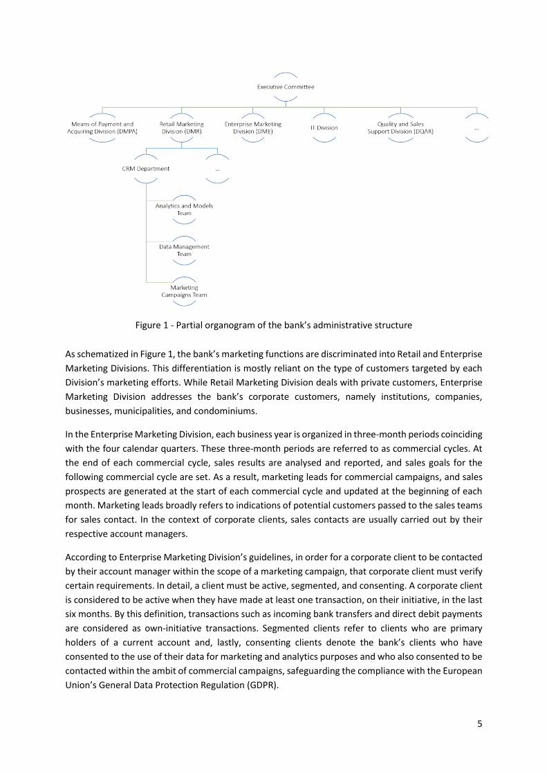
A partial organogram of the bank’s administrative structure is presented in Figure 1. Albeit not
including all functional units within the bank, all relevant teams and divisions mentioned throughout
this thesis have been included in this graph.
5
Figure 1 - Partial organogram of the bank’s administrative structure
As schematized in Figure 1, the bank’s marketing functions are discriminated into Retail and Enterprise
Marketing Divisions. This differentiation is mostly reliant on the type of customers targeted by each
Division’s marketing efforts. While Retail Marketing Division deals with private customers, Enterprise
Marketing Division addresses the bank’s corporate customers, namely institutions, companies,
businesses, municipalities, and condominiums.
In the Enterprise Marketing Division, each business year is organized in three-month periods coinciding
with the four calendar quarters. These three-month periods are referred to as commercial cycles. At
the end of each commercial cycle, sales results are analysed and reported, and sales goals for the
following commercial cycle are set. As a result, marketing leads for commercial campaigns, and sales
prospects are generated at the start of each commercial cycle and updated at the beginning of each
month. Marketing leads broadly refers to indications of potential customers passed to the sales teams
for sales contact. In the context of corporate clients, sales contacts are usually carried out by their
respective account managers.
According to Enterprise Marketing Division’s guidelines, in order for a corporate client to be contacted
by their account manager within the scope of a marketing campaign, that corporate client must verify
certain requirements. In detail, a client must be active, segmented, and consenting. A corporate client
is considered to be active when they have made at least one transaction, on their initiative, in the last
six months. By this definition, transactions such as incoming bank transfers and direct debit payments
are considered as own-initiative transactions. Segmented clients refer to clients who are primary
holders of a current account and, lastly, consenting clients denote the bank’s clients who have
consented to the use of their data for marketing and analytics purposes and who also consented to be
contacted within the ambit of commercial campaigns, safeguarding the compliance with the European
Union’s General Data Protection Regulation (GDPR).
6
1.2. PROBLEM DEFINITION
Customer-driven marketing strategies are geared towards identifying and meeting clients’ needs, as
well as targeting a specific market segment to reach the clients who would benefit the most from
certain products or services. To do so, such marketing strategies must leverage customer knowledge
in order to direct customers towards products and services that meet their current or future
requirements. Notwithstanding, extracting value from the extensive and varied volumes of data
available, while safeguarding the time-to-market and realizing customers’ expectations, has become a
complex challenge faced by marketing professionals. In light of this, companies have been integrating
machine learning functions in marketing processes. By transforming historical data into actionable
insights, these systems strive to automate, optimize and augment marketers’ productivity and work
efficiency, as well as to better anticipate customers’ behaviours and preferences.
Aiming at more efficient customer engagement, companies are striving to automate the choice of the
most appropriate offer to each customer as per their characteristics and needs. According to the
literature, one of the main approaches to tackle this problem are Recommender Systems. On this
thesis, such systems were studied for addressing the problem of automating financial product
recommendations to corporate clients, in the banking sector.
Problem Definition:
Automating the choice of which financial product to market for each corporate customer
On this basis, the following five research questions have been investigated:
(1) How can the most suitable financial product be recommended to a corporate client?
(2) Can exploratory data analysis provide insights into the prediction problem?
(3) Which predictive model performs best for the problem at hand?
(4) Would Feature Selection and Extraction methods improve model performance?
(5) Which prediction approach is best suited for recommending financial products to corporate
clients?

7
1.2.1. Case Study
This Subsection will cover the case study of the application of the selected approach to address the
problem of automating the choice of which financial product to market for each corporate customer,
in the banking sector.
As part of a set of initiatives launched to mitigate the shortage of integrated intelligent decision
technologies in Enterprise Marketing Division’s marketing processes, CRM Department’s Analytics and
Models team assumed the task of employing intelligent advanced analytics and predictive modelling
capabilities to boost marketing leads generation processes. In particular, aiming to assist sales teams
and account managers in identifying which second-level product should be suggested to each
corporate customer as part of the sales contact plan for each commercial cycle. As such, under the
scope of a research internship program, the development of a model identifying the most suitable
second-level product for each corporate customer was undertaken as the research subject for this
thesis.
Ultimately, information regarding the second-level product that is most likely to be bought by a specific
corporate customer will be passed as leads onto the respective account managers, who will be
responsible for contacting the customers. Therefore, the project goal revolves around anticipating
corporate clients’ needs and bettering the efficiency of sales representatives, thus leading to increased
corporate clients' satisfaction and profitability.
1.2.2. Constraints and Limitations
In this thesis, the data used for modelling and evaluating the proposed Recommender architectures
was provided by a Portuguese private commercial bank, as part of a research internship program. This
dataset, generated in accordance with the researcher’s access profile and authorizations, featured a
set of attributes pertaining to corporate clients identified by a pseudo-unique identification number.
Due to data security and privacy bank policies, customer name and other unique identifiers, such as
Taxpayer Identification Number, were pre-excluded from the provided real-life dataset, in compliance
with European Union’s General Data Protection Regulation (GDPR), as well as the bank’s confidentiality
and data protection policies.
Additionally, as part of the case study’s constraints, the developed Recommender System was required
to exclusively base its prediction upon the internal data provided by the bank. As such,
recommendation techniques and predictive algorithms were selected in accordance with the available
information.
Finally, respecting Enterprise Marketing Division’s business year organization and marketing leads
generation procedures, the implemented Recommender System’s independent variables were
required to regard a single commercial cycle (from now onwards referred to as the base commercial
cycle). In turn, the dependent variables were requested to review the acquisition patterns followed by
each corporate customer in the following commercial cycle, that is, in the three months following the
base commercial cycle. This period will henceforth be designated as target commercial cycle.

8
1.2.3. Proposed Solution
As per the case study’s constraints and limitations, a Collaborative-Demographic Hybrid
recommendation approach will be employed for predicting the most suitable second-level financial
product purchase for each corporate client.
According to the surveyed literature, this prediction task can be formulated as either a multi-output
regression or a multiclass classification problem. In a multi-output context, the prediction’s target for
each user is usually a vector of item ratings, denoting, for instance, item purchase likelihood. In a
multiclass classification problem setting, the product that is most likely to be bought by a specific
customer is selected from the range of available products. Recommenders following this prediction
approach are often referred to as Next-Product-To-Buy (NPTB) models (Bogaert et al., 2019).
In this thesis, both prediction approaches are implemented and compared. For multi-output
regression, the prediction’s target are 10-dimensional binary vectors denoting product purchases by
corporate clients during the target commercial cycle. In this scenario, each position in the 10-
dimensional binary vectors corresponds to a specific product class. The label associated with each
product class is set to 1 if a product belonging to that class was purchased during the target commercial
cycle, and 0 otherwise. Once the model is trained, it can be applied to predict item purchase likelihood.
Hence, values in the predicted vectors will range from 0 to 1. Thus, selecting the most suitable financial
product purchase for each corporate client u corresponds to solving 𝑎𝑟𝑔𝑚𝑎𝑥(𝑣𝑢), where 𝑣𝑢 is the
predicted vector for corporate client u (Choo et al., 2014). Alternatively, for multiclass classification,
the prediction’s target is defined as the first product acquired by each corporate client during the
target commercial cycle.
This thesis’ work has both theoretical and practical implications. Existing literature centred around
financial products recommendation in a corporate banking environment is limited. Thus, from a
theoretical point of view, this project supplements existing literature in two main aspects. First, it
proposes a system for financial product recommendation directed at corporate clients, and secondly,
it provides a comparison between multi-output regression and multiclass classification prediction
approaches. On a practical level, the impact of this research work is two-fold. First, it allows for higher
accuracy when targeting marketing campaigns by anticipating clients’ needs. On the other hand, the
proposed Recommender provides added value to account managers’ recommendations, and allow for
increased automation of sales and marketing leads generation processes.
The remainder of this thesis is organized as follows. Chapter 2 provides an overview of relevant
Recommendation Systems’ literature, including a brief outline of Recommenders’ evolution, as well as
a summarization of the Systematic Literature Review results. In Chapter 3, the CRISP-DM research
methodology is discussed, the utilized tools and technologies are briefly introduced, and some
theoretical notions behind the employed algorithms, implementation details and hyperparameter
tuning efforts are covered. In Chapter 4, data collection, preparation, and processing steps are
overviewed. In Chapter 5, Recommender’ performance results for both multi-output regression and
multiclass classification are presented and discussed, followed by a comparison between both
prediction approaches and a more in-depth analysis of the best overall model. Chapter 6 provides an
overview of preliminary deployment tasks, including a commercial viability assessment for the
proposed Recommender through ex-post backtesting, and an outline of the deployment. In Chapter 7,
overall conclusions, limitations, and future work directions and improvements are outlined.

9
2. THEORETICAL FRAMEWORK
This Chapter provides a discussion on the concepts that informed the study. In more detail, Section
2.1. presents an overview of relevant definitions and terminology, as well as a brief outline of
Recommenders’ evolution. In Section 2.2., different recommendation techniques are introduced.
Section 2.3. covers a categorization for Recommenders’ input features, and, in Section 2.4., implicit
rating structures are discussed. Lastly, in Section 2.5., the results of a Systematic Literature Review of
Recommender Systems, applied to the financial sector, are summarized and analysed in terms of the
year of publication, application domain, recommendation techniques, underlying algorithms, and
evaluation strategies and metrics employed.
2.1. RECOMMENDATION SYSTEMS
In this Section, relevant definitions and terminology for this thesis’ work are presented to provide the
necessary background knowledge about the studied themes. Additionally, Recommendation Systems’
evolution, since the first Recommender until promising future research directions will be overviewed.
2.1.1. Definitions and Terminology
Regarding terminology, throughout this thesis, the terms “Recommender”, “Recommender System”
and “Recommendation System”, as well as “client” and “customer” are used interchangeably. In the
context of Recommender Systems, the term “users” refers to entities that actively interact (e.g., view,
purchase, rate) with the different items in the system. In turn, items refer to the recommendable
objects with which the users can interact (e.g., movies, books, songs).
Several definitions of Recommender Systems can be found in the literature. Thorat et al. (2015)
generally defined Recommendation Systems as systems that suggest items in which the users might
be interested. Other broad definitions are provided by Bogaert et al. (2019), who state Recommender
Systems are able to convert user preferences into predictions of their interests, and Zhang et al. (2019)
affirmed Recommender Systems proactively recommend items based on estimates of users’
preference.
Other definitions emphasize the underlying technologies of the recommendation process. Zibriczky
(2016) defined Recommender Systems as “information filtering and decision supporting systems that
present items in which the user is likely to be interested”. Park et al. (2011) remark the use of analytic
technology to compute purchase probability in order to recommend the right product for each user.
More generally, Çano and Morisio (2017) define Recommender Systems as “software tools and
techniques used to provide suggestions of items (…) to users”.
In sum, previous interpretations were combined to create the Recommendation Systems’ definition
underlying this thesis’ work. Henceforth, Recommenders will be taken as systems leveraging user and
item data for suggesting the item or items in which each user is likely to be most interested.

10
2.1.2. Recommendation Systems’ Evolution
In the last 30 years, with the evolution of the web, and the advent of digital information, the amount
of data available grew exponentially (Çano & Morisio, 2017). This scenario originated an information
overload phenomenon, with users having increased difficulty sifting through the vast amounts of
content available in order to locate the right information at the right time (O’Donovan & Smyth, 2005).
In this context, Recommender Systems emerged in the early 1990s as an information filtering tool to
mitigate this problem (O’Donovan & Smyth, 2005; Zhang et al., 2019). The first research paper on
Recommender Systems (Sinha & Dhanalakshmi, 2019) featured a Collaborative Filtering technique
designed to filter electronic documents as per their alignment with the user’s interests (Goldberg et
al., 1992). Other prototypes applying Collaborative Filtering emerged in the mid-1990s. Among them,
GroupLens, a recommendation engine for news articles filtering, and Ringo, which provided
personalized music recommendations according to users’ musical taste similarities (Çano & Morisio,
2017).
As an independent research field closely related to Information Retrieval, Machine Learning, and
Decision Support Systems (Jannach et al., 2012), Recommendation Systems have received significant
attention from both researchers and practitioners during the past years (Jannach et al., 2012). This
growing academic and industrial interest was prompted by several factors (Jannach et al., 2012).
Among them highly visible innovation competitions such as the Netflix Prize 1, the rapid growth of e-
commerce and Internet-based companies (Lü et al., 2012) and the rising importance of providing users
with the most relevant personalized content and services amid the explosive growth in the amount of
available information and stricter customer expectations (Abdollahpouri & Abdollahpouri, 2013).
In the early years, Recommender Systems primarily relied on an explicit rating structure (Adomavicius
& Tuzhilin, 2005). However, with the growing volume of information available (Zhang et al., 2019),
Recommendation Systems started to follow a clear tendency to integrate more diverse types of data,
namely through hybridization techniques (Gunawardana & Meek, 2009). Currently, due to advances in
the Social Web and mobile environment (Çano & Morisio, 2017), these hybrid systems are
incorporating social and contextual information (e.g., location, time), with authors predicting an
increase of applications employing Social Network Analysis (Park et al., 2011), and Context-Aware
(Barranco et al., 2012) Recommendation Systems.
2.2. RECOMMENDATION TECHNIQUES
Recommendation techniques refer to the underlying paradigms supporting the computation of
personalized recommendations (Jannach et al., 2012). Former works (Sharifihosseini & Bogdan, 2018;
Burke, 2007) have classified recommendation techniques into Content-Based, Collaborative,
Demographic, Knowledge-Based, and Hybrid approaches. This categorization builds upon the
knowledge sources feeding the recommendation process (Burke, 2007).
1 Netflix Prize, [Online]. Available: https://www.netflixprize.com/

11
2.2.1. Content-Based Recommenders
Content-Based Recommendation is rooted in research fields of Information Retrieval (Adomavicius &
Tuzhilin, 2005) and Information Filtering (Burke, 2002). These approaches are grounded on the
premise that a user will be interested in items which are similar to the ones the user bought, consumed,
or rated positively in the past (Thorat et al., 2015).
Content-Based Recommenders rely on profiles of the users’ preferences. This profiling information can
be obtained explicitly (e.g., via user forms or questionnaires) or implicitly, through the analysis of the
attributes of items previously rated by the user as well as the user’s historical transactional data. Upon
constructing a portfolio of user interests, Content-Based approaches match the properties of each
candidate item with the established preference profile of each user (Choo et al., 2014). In the end, the
items that best fit the user’s interests are recommended.
Content-Based Filtering is mainly designed to recommend text-based items (Adomavicius & Tuzhilin,
2005), that is, items with inherent textual content (e.g., news articles, web pages, documents) as well
as items whose description integrates information extracted from web environments, such as
comments, posts, and tags. As such, in these systems, the item descriptions are usually represented
by keywords, with Term Frequency/Inverse Document Frequency (TF-IDF) being the most extensively
employed technique (Thorat et al., 2015) to support the recommendation process.
Contrary to Collaborative Filtering, Content-Based Recommender Systems do not require data from
other users, and they are able to suggest unpopular or new items, so as long as they have item features
associated. Content-Based approaches are dependent on the item descriptions and features. As such,
the unavailability of item features, inherent to a certain domain, constitutes a significant impairment
to the application of Content-Based Filtering methods.
Since Content-Based recommendations are reliant on a user’s past preferences, in cases where the
user has yet to rate a sufficing amount of items, the system will not be able to produce accurate
recommendations. This is usually referred to as the New User Problem, a ramification of the Cold-Start
Problem or Ramp-Up Problem (Burke, 2002).
Due to the content-oriented approach of recommending items on the basis of how similar they are to
the ones the user previously preferred, Content-Based Filtering suffers from overspecialization, only
being able to recommend items akin to those the user has already consumed or bought (Park et al.,
2011). This limitation is particularly critical in certain domains (e.g., news articles) where items should
not be recommended if they are too similar to items the user is already aware of (Adomavicius &
Tuzhilin, 2005).
Another challenge that arises from the application of Content-Based approaches is the plasticity
problem, meaning that once a preference profile has been ascertained for a user, it is difficult to shift
the user’s preferences (Burke, 2002). As such, and by way of example, a user that recently became a
vegetarian will continue to receive recommendations for steakhouses if said user has positively rated
similar restaurants in the past.

12
2.2.2. Collaborative Filtering
Content-Based and Collaborative Filtering are the most pervasive recommendation techniques found
in the literature (O’Donovan & Smyth, 2005), with Collaborative Filtering being the most extensively
used and most mature approach (Thorat et al., 2015).
The phrase “Collaborative Filtering” was first coined by the developers of the first Recommender
System, Tapestry (Renick & Varian, 1997; Sharifihosseini & Bogdan, 2018). Collaborative
recommendation is grounded on the assumption that users who shared similar preferences in the past
will continue to have similar tastes in the future. As such, Collaborative Filtering recommendations rely
on the items favoured by the users considered to have the most in common with the target user.
This type of Recommender Systems is grounded on user-generated feedback, which can be extracted
explicitly (e.g., through item ratings or like/dislike indicators) or implicitly (e.g., by collecting browsing
history, or historical data of consumed content) (Zhang et al., 2019; Mohamed et al., 2019). With this
information about the users’ past interactions, the system builds user rating profiles (i.e., vectors of
item ratings), which are continuously complemented over time by the user’s interactions with the
system. All these user profiles are then aggregated into a User x Item matrix, which supports the
identification of taste commonalities between users.
In order to provide suitable recommendations, Collaborative approaches compare the rating profiles
in order to identify the users who rated products in a similar way to that of the target user (Thorat et
al., 2015). Thereupon, each user will be recommended items that other users with similar preferences
rated positively in the past. k-Nearest Neighbours (kNN) is the most widely used algorithm for
implementing Recommendation Systems based on Collaborative Filtering paradigms (Thorat et al.,
2015).
Collaborative Filtering systems can be classified as either Model-Based or Memory-Based (also called
Heuristic-Based) (Lü et al., 2012). Model-Based systems learn a model from the User x Item rating
matrix, which is then used to make predictions (Xue et al., 2017). On the other hand, Memory-Based
recommendations result from directly comparing users by means of similarity or correlation measures
calculated over the entire rating collection (Burke, 2002), which must remain available in the system’s
memory during the algorithm’s runtime.
One of the most significant advantages of Collaborative Filtering techniques over Content-Based
methods is its ability to generate cross-genre recommendations. For instance, Collaborative algorithms
can provide novel or “outside the box” suggestions for a comedy genre aficionado, by discovering that
users who enjoy comedy also enjoy horror movies (Burke, 2002). Collaborative methods do not require
domain knowledge or data about either users or items in order to make suggestions.
Collaborative Recommender Systems suffer from sparsity problems (Park et al., 2011), which arise
when users rate only a minimal amount of available items. Sparse rating matrixes are usually
associated with domains having exceedingly large item spaces (Lü et al., 2012). That is, since these
techniques depend on the intersection of ratings across users, sparse User x Item rating matrixes
negatively impact the generation of quality recommendations (Park et al., 2011). The sparsity problem
is attenuated to a certain extent in Model-Based approaches (Burke, 2002).

13
Collaborative Filtering Recommenders also suffer from the Cold-Start (or Ramp-Up) Problem, which
branches into the New Item and New User problems. In certain domains where new items are regularly
added to the system or when some items go unrated due to the large item space, Collaborative
systems would not be able to recommend such items until they gather a sufficient amount of user
ratings. This problem is referred to as the New Item problem (Adomavicius & Tuzhilin, 2005; Sinha &
Dhanalakshmi, 2019). The New User problem, on the other hand, relates to Collaborative Filtering’s
reliance on the accumulation of ratings for inferring about users’ past preferences. Consequently,
Collaborative Filtering systems cannot provide reliable recommendations for new users who have yet
to rate a sufficient amount of items to enable the system to extrapolate their preferences (Thorat et
al., 2015).
Additionally, with new items having very few ratings, it is unlikely for Collaborative approaches to
recommend them and, in turn, items that are not recommended may go unnoticed by most users who,
consequently, do not rate these items. This cycle can, therefore, lead to unpopular items being left out
of the Collaborative recommendation process (Bobadilla et al., 2013). Collaborative approaches also
suffer from the grey sheep problem (Mohamed et al., 2019). For users with unusual preferences among
the population, Collaborative approaches may not find users with similar profiles, thus leading to a
poor recommendation.
2.2.3. Demographic Filtering
One way to mitigate the rating sparsity problem of Collaborative approaches is to exploit additional
user information, namely demographic characteristics when calculating user similarity (Lü et al., 2012).
Demographic-Based Recommenders assume that users belonging to the same demographic segment
(i.e., users sharing certain personal attributes) will have common preferences (Bobadilla et al., 2013).
Pure Demographic-Based systems adopt a similar approach to Collaborative Filtering, as they provide
recommendations on the basis of user profile comparison. However, these systems take as input users’
personal attributes instead of historical rating data.
Another approach is to employ Demographic Filtering as an extension of Collaborative Filtering, with
users being considered similar not only if they have similarly rated the same products but also if they
have certain personal attributes in common (Mohamed et al., 2019). In such cases, Demographic
Filtering is considered a reinforcing technique to improve recommendation quality (Çano & Morisio,
2017).
Unlike Collaborative Filtering, pure Demographic-Based Recommenders do not suffer from the New
User problem, as they do not require historical data about user ratings. In turn, they depend on users’
personal information whose collection gives rise to privacy concerns.

14
2.2.4. Knowledge-Based Recommenders
Knowledge-Based Recommenders are based on knowledge structures, namely cases, and constraints
(Bobadilla et al., 2013). These systems provide recommendations by reasoning about what items
comply with the elicited requirements. User requirements are usually collected by means of a
knowledge acquisition interface. The need for knowledge acquisition is the biggest shortcoming of
Knowledge-Based systems (Adomavicius & Tuzhilin, 2005).
Knowledge-Based systems can be further differentiated into Case-Based and Constraint-Based
systems. Case-Based systems apply Case-Based Reasoning (CBR) to address the recommendation
problem. Case-Based Reasoning is a lazy learning technique that relies on the assumption that similar
problems have similar solutions (Leonardi et al., 2016). Thus, CBR approaches a new problem (i.e.,
target case) by recalling, reusing, or adapting the solution of similar past cases (Sinha & Dhanalakshmi,
2019). Previously solved problems and their respective proposed solutions are stored in a Case Library
(Musto et al., 2015).
Constraint-Based Recommenders are grounded on a set of explicitly defined constraints regarding user
and legal requirements for item properties. Such constraints are also denoted as filter constraints
(Felfernig, 2016). On this basis, Constraint-Based methods recommend to the user a set of items that
fulfil the constraints elicited, by filtering the items whose properties are compliant with the given
requirements.
2.2.5. Hybrid Recommenders
Hybrid Recommenders refer to systems that integrate two or more recommendation approaches
(Zhang et al., 2019). In the late 1990s, researchers started to combine Recommenders in order to
exploit their complementary advantages (Çano & Morisio, 2017). The primary motivation for the
combination of different techniques and knowledge sources (Jannach et al., 2012) is two-fold. Hybrid
Filtering approaches aim to improve recommendation performance while overcoming or alleviating
the drawbacks associated with individual recommendation techniques (Mohamed et al., 2019), in
particular, the Cold Start problem. Hybrid Filtering systems are usually implemented using bio-inspired
or probabilistic methods, namely neural networks and genetic algorithms (Bobadilla et al., 2013).

15
2.3. RECOMMENDATION SYSTEMS’ INPUT FEATURES
According to Sinha and Dhanalakshmi (2019), input information provided to the Recommendation
System can be classified as:
Socioeconomic data, including population characteristics such as gender, date of birth and income
for retail customers , or sector of economic activity, sales volume and number of employees for
corporate clients;
Behaviour pattern data, including indicators of interaction patterns between users and items,
namely website clicks, amount of time spent browsing and number of visualizations;
Proceedings data, describing events featuring a time dimension (e.g., purchasing details such as
purchase timestamp, quantity, price, and discount);
Production informative data, of which the most significant example is items’ content descriptions;
Rating data, that is, indications or quantifications of users’ perceived item quality.
In addition to the aforementioned input data categories, financial indicators of the clients’ relationship
with the bank (Urkup et al., 2018), such as number of years as customer and Share of wallet, were also
included in this thesis.
2.4. IMPLICIT RATING STRUCTURES
Ratings constitute indications or quantifications of users’ perceived item quality. These ratings can be
binary remarks (e.g., like/dislike) or interval scales specifying a degree of preference (Burke, 2002). In
most cases, rating information is explicitly collected. However, ratings can also be implicitly acquired
by considering certain user-item interactions, namely item purchase and consumption (Lü et al., 2012).
Implicit preference elicitation is based on the inference of facts about the user on the basis of their
observed behaviour (Rashid et al. 2008). For example, we can consider a binary User x Item matrix
where the rating 1 in the position (u, i) signifies the user u has purchased the item i. The downside of
this approach is the ambiguity of the resulting negative instances (i.e., zero ratings), as they can be
interpreted in two ways; either the user is not interested in the items or the user does not know about
them (Bogaert et al., 2019).

16
2.5. SYSTEMATIC LITERATURE REVIEW
To better understand the scientific background framing this work, as well as to adequately position its
contributions, a review of the state-of-the-art of Recommender Systems research was undertaken.
Reported review work conclusions resulted from the application of Systematic Literature Review (SLR)
guidelines. Details into the methodology adopted, Review Protocol established, and different phases’
output can be consulted in Appendix D.
During this review work, the state-of-the-art of Recommender Systems, applied to the financial sector,
was summarized and analysed in terms of the year of publication, application domain,
recommendation techniques, underlying algorithms, and evaluation strategies and metrics. In this
Section, a brief summary of the key conclusions drawn from the application of an SLR methodology to
analyse relevant Recommendation Systems literature will be provided. For a detailed overview of the
review work’s conclusions, refer to Appendix D.
First, with regard to the Data Mining and Machine Learning (DM/ML) techniques employed by
Recommendation Systems, a wide variety of techniques is used for Recommender’s implementation,
with authors typically using diverse approaches when building the different components of the
proposed Recommendation System architecture. Amongst them, the most frequent technique is
found to be reliant on the calculation of distance or similarity measures for producing item
recommendations. However, around 27% of the reviewed studies implement only one machine
learning algorithm in their Recommendation System solution. Particularly, Association Rule Mining,
Neural Networks, Ensemble regressors and classifiers, Correlation Coefficients, and Matrix
Factorization techniques.
Additionally, about 10% of the reviewed studies explicitly reported having used feature
selection/extraction (FSE) methods to lessen the number of variables under consideration, aiming to
efficiently summarize the input data, reduce the computational requirements, or enhance the
predictive model’s performance. Some of the employed FSE methods include Recursive Feature
Elimination (RFE), Forward and Backward Selection, f_regression, Principal Components Analysis
(PCA), and Non-Negative Matrix Factorization (NMF).
Finally, five problem classes were identified for recommending the most suitable item(s) for each user:
binary classification, multi-class classification, multi-label classification, single-output regression, and
multi-output regression.
Binary classification tries to ascertain whether each user will consume or purchase a particular item.
Application examples found for this class of problems are predicting whether a lender will fund a loan,
whether a bank customer will apply for/subscribe/acquire a specific product, and whether a news
article is relevant.
Still considering Recommenders suggesting only one product for each user, multi-class classification
problems select, out of the whole range of products, the one that is most likely to be bought by a
specific customer. Amidst the reviewed studies structured as multi-class classification problems, the
target was considered, for instance, as the last financial product purchased by each customer. In turn,
Multi-label classification selects a set of the k products most likely to be of interest to the user,
considering the whole range of available products. Amid the primary studies considered, multi-label

17
classifiers were used to recommend a set of financial products for cross-sell purposes, to automatically
find potential lenders, in a P2P lending environment, for the target loan, and to identify the most
appropriate service selection, in order to adjust the menu ordering in banking applications.
Regarding regression problems, single-output regression was employed mostly to predict stock
prices/expected stock returns. However, it was also utilized in other application domains, such as P2P
lending, where it was used to predict the likelihood of funding for a given (lender; loan) pair. In this
case, the best lender for a particular loan i can be found by solving argmaxi (U, i) for all users in the U
set. Analogously, the most suitable loan for a lender u to invest in can be found by calculating the
argmaxu (u, I) for all loans in the I set.
Lastly, multi-output regression problems are primarily used for predicting a vector of item
consumption/acquisition probabilities for each user. For instance, in the field of Financial Statements
Auditing, a Feed-Forward Neural Network was proposed for mapping each passage from the financial
statement under audit (i.e., considered the “user” of the Recommendation System) to a relevance
vector for all the legal requirements (i.e., the recommended items).
Then, with regard to the recommendation techniques found on the set of primary studies reviewed,
Content-Based and Collaborative Filtering were the most frequently employed techniques for
recommendation computation.
Furthermore, for providing a more integrated perspective, the distribution of DM/ML techniques was
analysed according to the underlying recommendation technique. This analysis emphasised that the
use of certain DM/ML techniques is highly dependent on the recommendation paradigm employed,
with Correlation Coefficients found to be exclusively used with Collaborative Filtering approaches. In
contrast, Time Series Analysis was employed only in Content-Based Recommenders.
From this analysis, it was possible to denote that Collaborative Filtering approaches mostly rely on Rule
Mining, Correlation computation, K-Nearest Neighbours algorithm, and Matrix Factorization methods.
While Content-Based approaches, mainly due to the need for item properties extraction, focus on
Word Embedding and Text Vectorization techniques, Knowledge Representation mechanisms (such as
Ontologies), and Time Series Analysis.
In addition, the Recommenders’ evaluation process was examined with regard to the evaluation
methodologies and metrics adopted. For this topic, most studies reported having evaluated the
proposed algorithm(s) in comparison against one or more baselines, usually chosen from the most
widely implemented algorithms (e.g., kNN, MF) for the recommendation paradigm being employed.
The second most used evaluation methodology relies on comparing either different parameter
configurations or variations of the proposed Recommender. That is, for instance, Recommenders
relying on different Feature Selection/Extraction techniques, different classifiers or regressors, and
different recommendations ranking strategies.
Among the considered primary studies, 16 report having split their dataset into train and test sets
when assessing the Recommender’s performance. Cross-validation was performed in 8 studies, and
backtesting was employed in two Recommenders for the Stock Market domain. User studies and
surveys were used in 4 cases, while comparison against domain experts was undertaken in 3 studies.
Both these evaluation methodologies require the involvement of users who perform mainly subjective

18
quality assessments and provide feedback about their perception of the Recommendation System.
Finally, from the 8 primary studies which did not report evaluation, two indicated the evaluation of
their recommendation framework as future work.
Regarding the metrics involved in the evaluation methodology, the most common metrics used for
Recommenders’ evaluation are classification measures such as Recall, Precision, Accuracy, Area Under
the ROC curve (AUROC), F-Measure and Mean Average Precision (MAP), Specificity, Mean Reciprocal
Rank (MRR) and G-Mean. For regression problems, the most frequently used error measure is Root
Mean Square Error (RMSE). Trailing error measures include R-Square and Mean Absolute Error (MAE).
To complement the aforementioned accuracy measures, novelty and diversity metrics have been
proposed and employed in a 4 studies. Further, among the considered primary studies, algorithms’
runtime was evaluated in 3 studies, and scalability assessment was explicitly carried out on one paper.
Dispersion measures, such as Median Absolute Deviation (MAD), were present in 4 primary studies.
Several of the considered primary studies have also reportedly assessed their Recommenders on the
basis of financial/economic indicators such as the yield, gain, profit, and Return On Investment (ROI)
obtained from the recommended item, particularly stocks and investment portfolios.
Some problem- and algorithm-specific metrics were evaluated in 5 primary studies. Included metrics
in this category are, for instance, the number of atoms per dictionary [P19]. Usability and Domain
Experts' opinions were employed as evaluation metrics in primary studies performing user and domain
expert-based studies, respectively.

19
3. METHODOLOGY
In this Chapter, the research methodology adopted for this thesis’ data mining project development is
reviewed. Section 3.1. presents a summarized description of each CRISP-DM phase, as well as a
detailed overview of their tasks and respective outputs. Section 3.2. briefly introduces the tools and
technologies utilized throughout this project. Finally, Section 3.3. covers some theoretical notions
behind the employed predictive models and FSE methods, complemented by examples of studies
applying these algorithms, as well as implementation details and hyperparameter tuning efforts.
3.1. RESEARCH FRAMEWORK
The data mining methodology used in this thesis is the Cross-Industry Standard Process for Data Mining
(CRISP-DM). In terms of data mining process models and methodologies, CRISP-DM is considered the
de facto standard for developing data mining projects (Martínez-Plumed et al., 2019). Furthermore,
alongside SEMMA, it is one of the most popular industry standards for the implementation of data
mining applications (Azevedo & Santos, 2008; Shafique & Qaiser, 2014). However, unlike the Sample,
Explore, Modify, Model, Assess (SEMMA) model, which was developed by the SAS institute (Shafique
& Qaiser, 2014) as “a logical organization of the functional toolset of the SAS Enterprise Miner”
software (Marbán et al., 2009), CRISP-DM is independent of the project’s application domain, and
technology tools used. (Wirth & Hipp, 2000; Marbán et al., 2009)
The CRISP-DM process was developed in the mid-1990s (Marbán et al., 2009) by a European funded
consortium (Martínez-Plumed et al., 2019) composed by DaimlerChrysler, Teradata, OHRA, SPSS and
NCR (Azevedo & Santos, 2008; Shafique & Qaiser, 2014; Marbán et al., 2009). The first version of CRISP-
DM, providing a uniform framework and guidelines for planning and conducting data mining projects,
was published in 1999 (Shafique & Qaiser, 2014).
CRISP-DM builds on previous attempts to define knowledge discovery methodologies (Wirth & Hipp,
2000). Aiming to provide a uniform and structured approach to data mining projects development,
CRISP-DM reference model overviews the life cycle of a data mining project, consisting of six well-
defined phases, their respective tasks, and outputs (Wirth & Hipp, 2000; Shafique & Qaiser, 2014).
A brief description of the CRISP-DM’s phases is presented below.
Business Understanding
During this phase, the focus is on understanding the project’s requirements and business objectives.
Additionally, elements such as success criteria and relevant domain knowledge and terminologies
should be elicited. Then, in view of the acquired insights, a data mining problem definition should be
formulated.
Data Understanding
During this phase, the data is collected and explored, allowing for proper familiarization with the data,
namely in regard to data quality and interesting subsets or underlying patterns. In sum, the first
insights into the available data are formulated during this phase.

20
Data Preparation
This phase encompasses all the steps undertaken to construct the processed dataset that will serve as
input for modelling the algorithm(s). Usual data preparation tasks are record, and attribute selection,
data cleaning, new attribute construction, and attribute transformation.
Modelling
In this phase, the appropriate data mining task (e.g., binary classification, multiclass classification,
clustering, regression) is identified, and corresponding data mining and machine learning algorithms
are selected, implemented, and fine-tuned. Typically, several techniques are considered for modelling
the same data mining problem.
Evaluation
After implementation and parameter calibration, the algorithms’ performance must be thoroughly
evaluated. Additionally, during this phase, the constructed architecture should be reviewed in order
to guarantee that the project’s objectives, defined during the business understanding phase, are being
achieved.
Deployment
This phase focuses on organizing, reporting, and presenting the discovered knowledge so it can be
used by the interested parties. Furthermore, this phase can also entail the integration of the proposed
architecture into another system, as well as subjacent monitoring and maintenance.
A more detailed overview, entailing the generic tasks for each CRISP-DM phase, as well as their
respective outputs, can be seen in Figure 2.
Figure 2 - CRISP-DM Reference Model’s phases, respective tasks, and outputs
Adapted from (Chapman et al., 2000). Generic CRISP-DM phases’ tasks are represented
in bold, and corresponding outputs are presented in italic.

21
The sequence of CRISP-DM phases is not strict. In practice, it will often be necessary to backtrack to
previous phases and repeat certain tasks as a response to the outcome of each phase (Wirth & Hipp,
2000). The most frequent dependencies between project phases are schematized in Figure 3.
Figure 3 - Most frequent dependencies between CRISP-DM project phases
Adapted from (Chapman et al., 2000).
The six phases of the CRISP-DM methodology provide a framework for this thesis’ research. Business
Understanding tasks’ outputs, namely project context, requirements, and problem definition, were
provided in Chapter 1. Data Understanding outputs, in particular, data collection, dataset description,
as well as first insights into the data, were provided in Sections 4.1. and 4.2. Data Preparation tasks,
and their respective results, are detailed in Section 4.3. Modelling phase’s algorithm selection task, as
well as models’ construction and hyperparameter tuning efforts are reported in Section 3.3. Model
evaluation is addressed in Chapter 5. Lastly, preliminary tasks of the Deployment phase are covered in
Chapter 6.

22
3.2. TOOLS AND TECHNOLOGIES
In this thesis, Python will be used as the main tool for analytics and data mining. Python is an open-
source general-purpose programming language created by Guido Van Rossum in 1991 (Brittain et al.,
2018). Due to a vast community of users, Python has been continuously evolving and extending its
capabilities through a collection of community-contributed packages. The Python Package Index
(PyPI)2 hosts thousands of Python packages, providing support for efficient storage and data
manipulation, as well as implementations of state-of-the-art machine learning algorithms, among
other tasks. In recent years, Python has been gaining momentum, reportedly surpassing popular
programming languages such as Java (Ozgur et al., 2017; Cass, 2019).
In the field of Data Science, alongside R and SAS, Python is also one of the prevalent coding languages
(Ozgur et al., 2019). In a recent survey, NumPy and Scipy packages were found amongst the most
popular for statistical analysis, while Scikit-Learn emerged as the preferred data mining package
(Brittain et al., 2018). In addition, as a general-purpose programming language (Ozgur et al., 2017),
Python has an edge over R with regard to model deployment, since it can more effectively integrate
the proposed model with other systems.
Even though Python was used as the main data science tool, R software was employed on occasion,
namely for constructing more informative visualizations ("Choosing Python or R for Data Analysis? An
Infographic", 2020) and for implementing algorithms not yet available on Python libraries. The R
environment, created by Robert Gentleman and Ross Ihaka, in 1993 (Ozgur et al., 2017), is an open-
source integrated suite of software facilities for data manipulation, calculation, and graphical display3.
Similarly to Python’s PyPI, the Comprehensive R Archive Network (CRAN) provides supporting
documentation and libraries with add-on packages (Brittain et al., 2018).
The data repository made available for this project consists of a set of SAS tables, the default SAS
storage format ("Choosing Python or R for Data Analysis? An Infographic", 2020). Thus, Base SAS was
employed for data collection. Base SAS Software is the core of Statistical Analysis System (SAS)4, a
proprietary set of software solutions developed by the SAS Institute. Base SAS Software offers a SAS
programming language for data access and manipulation, analysis, and reporting (SAS Institute Inc.,
2010).
Regarding Integrated Development Environments (IDE), the Jupyter Notebook web-based interactive
environment 5 was utilized for data exploration and visualization tasks, leveraging its notebook
document format for combining code, rich text, images, mathematical equations, and plots into a
single document.
PyCharm6 is one of the most frequently used IDEs for data science projects (Brittain et al., 2018). In
this thesis, data preparation, modelling, and evaluation tasks were carried out on PyCharm on account
of its intelligent coding assistance, providing smart code navigation and code completion; and also due
2 Python Software Foundation, [Online]. Available: https://www.python.org/. 3 The R Project, [Online]. Available: https://www.r-project.org/. 4 SAS Institute, [Online]. Available: https://www.sas.com/en_us/home.html. 5 Project Jupyter, [Online]. Available: https://jupyter.org/. 6 PyCharm, [Online]. Available: https://www.jetbrains.com/pycharm/.

23
to PyCharm’s Version Control Systems (VCS) integration and support, in particular the “Resolve
Conflicts” feature.
SAS Windowing Environment was used in this thesis for data retrieval and collection operations. While
RStudio, one of the most frequently used R language IDEs, was selected to carry out punctual tasks
involving R code (Brittain et al., 2018). Software version specifications for the different tools,
technologies, and IDEs employed in this thesis are presented in Table 1.
Table 1 - Software version specifications
Tools and IDEs Version
Python 3.6.6
SAS 9.2
R 3.4.3
Jupyter Notebook 6.0.1
PyCharm 2018.3
RStudio 1.1.456
As reported in Table 1, SAS Software’s version 9.2, released on March 1st, 2008, was employed for data
collection purposes. Albeit more recent versions having been released, the equipment provided by the
bank for accessing their data repository only featured the aforementioned SAS Software version. Thus,
Base SAS 9.2 was employed for data extraction tasks.
3.3. ALGORITHMS
In this Section, some theoretical notions behind the employed algorithms will be overviewed.
Additionally, examples of studies applying these algorithms, alongside obtained results, will be
presented. Further, the learning algorithms’ implementation details and hyperparameter tuning
efforts will be described.
For implementing this thesis’ Collaborative-Demographic Hybrid Recommender, four algorithms were
selected on account of their widespread usage according to the performed SLR of Recommendation
Systems applied to the financial sector. Additionally, two distinct Feature Selection and Extraction
methods were employed for improving Recommender performance.
Hyperparameter tuning was performed prior to the models’ evaluation, mostly through grid search.
Grid search is amongst the most widely used strategies for hyperparameter optimization. With this
approach, estimator performance is exhaustively evaluated over specified parameter values. Grid
search parameter optimization was performed using Python’s sklearn.model_selection.GridSearchCV
class with 5-fold cross-validation. With this setting, for each of the considered learning algorithms, a
5-fold cross-validated grid search over a user-defined parameter-grid was executed. The specified
hyperparameter grids can be found in Annex B. In order to find a good initial range of parameter values
for grid search tuning, preliminary ad-hoc experiments were carried out.

24
3.3.1. k-Nearest Neighbours
k-Nearest Neighbours (kNN) is a lazy or instance-based non-parametric algorithm. That is, for the
purpose of the prediction task, kNN directly searches through all the training data instances instead of
building a model (Dreiseitl & Ohno-Machado, 2002).
This algorithm is based on the premise that the most similar data points to a target (i.e., the target’s
neighbours) carry useful information for predicting the target’s label (Kramer, 2013). Therefore, the
kNN algorithm calculates the distances between all of the training data points and the target in order
to identify its k nearest neighbours.
Thus, for regression problems, the label assigned to the target is computed based on the mean or
median of its k nearest neighbours’ labels. While for classification problems, it is assigned based on
the most common class label among the target’s nearest neighbours (Brown & Mues, 2012).
The size of the considered neighbourhood is defined by k, one of the model’s hyperparameters. In
order to compute the target’s neighbourhood, that is, the k data points most similar to the target (i.e.,
the target’s nearest neighbours), it is necessary to define a similarity measure. A commonly used
distance for q-dimensional data spaces IRq is the Minkowski metric (Kramer, 2013), which corresponds
to the Manhattan distance for p=1 and to the Euclidean distance for p =2.
‖𝑥′ − 𝑥𝑗‖𝑝
= (∑ |(𝑥𝑖)′ − (𝑥𝑖)𝑗|𝑝𝑞
𝑖=1 )1
𝑝⁄ (1)
One of kNN’s drawbacks relates to its sensitivity to the value of k, which determines the locality of the
algorithm. For small values of k, the predictions are highly affected by noisy instances, while large
values of k result in smoother decision boundaries and increased computational expenditure (Ertuğrul
& Tağluk, 2017). Additionally, kNN is negatively affected by high dimensional spaces (Kouiroukidis &
Evangelidis, 2011). Thus relaying the importance of feature engineering methods, namely feature
selection and extraction.
The kNN algorithm is one of the most widely used prediction algorithms. Thus, it is frequently used as
a baseline in many domain problems. In Recommender System’s research, kNN is the most extensively
used Collaborative Filtering algorithm. As a model, kNN has been employed, for instance, for informing
venture investment decision-making by producing a list of the top-N investment opportunities for
Venture Capital firms and their investment partners [P51]. In this study, a dataset of 21.610 items (i.e.,
the private investee companies), 7560 Venture Capital firms, and 32.710 investment partners (i.e., two
distinct sets of users) was considered. Different system architecture configurations were tested, with
authors reporting a linear ensemble of kNN with 3rd tier (highest granularity) industry hierarchy
information as the best model, scoring an AUROC of 0.6582 and 0.6312, for Venture Capital firms and
investment partners, respectively.

25
Implementation Details
k-Nearest Neighbours (kNN) learning algorithm has been implemented with the help of sklearn’s
KNeighborsRegressor and KNeighborsClassifier, for the multi-output and multiclass prediction tasks,
respectively.
The choice for the values of kNN’s hyperparameters was data-driven. That is, the value of each
hyperparameter was set on the basis of kNN’s performance, assessed over a 5-fold cross-validated
grid-search optimization strategy. kNN’s hyperparameter grid dictionary used for Python’s cross-
validated grid search can be found in Annex B.
kNN algorithm’s tuned hyperparameters included the number of neighbours (n_neighbors), the
Minkowski distance power parameter (p), and the weight function (weights). For the power parameter
p, when it assumes the value 1, kNN will employ the Manhattan distance to compute the target’s
neighbourhood. Conversely, for p=2, the Euclidean distance will be used. With regard to the weighting
function, if a uniform weighting strategy is employed, all data points in the neighbourhood will
contribute equally to the prediction. If, on the other hand, distance weighting is used, the impact of
each neighbour’s contribution to the prediction will be the inverse of their distance so that closer
neighbours have greater influence than more distant ones.
The final configuration of hyperparameters resulting from the execution of the 5-fold cross-validated
grid search for KNeighborsRegressor and KNeighborsClassifier lead both models to be configured to
use the Manhattan distance to compute the target’s neighbourhood. In addition, for
KNeighborsRegressor, 100 data points were selected to constitute the target’s neighbourhood, while,
for KNeighborsClassifier, only 75 neighbours will be considered. Furthermore, KNeighborsRegressor
was configured with a uniform weighting strategy and, in turn, KNeighborsClassifier will be using
distance weighting.

26
3.3.2. Random Forest
Random Forest is a nonparametric tree-based algorithm belonging to the family of bagging ensemble
methods. In general, ensemble methods combine the predictions of a number of base learners in order
to improve the generalization ability and robustness when compared to a single base learner’s
performance.
Two popular ensemble methods are (Sutton, 2005): (1) boosting methods, where weak base learners
are iteratively built from weighted training samples. In each iteration, the weights are adjusted to give
increasing weight to cases which were misclassified in the previous iteration; (2) and bootstrap
aggregation, or bagging, methods, where a number of base learners are independently trained on
bootstrap samples drawn from the available data, and then their individual predictions are aggregated
to obtain the overall prediction.
For the particular case of Random Forests, each independent tree base learner is grown to full size
(i.e., no pruning) and fitted on a training sample, drawn with replacement, that is the same size as the
original training dataset (i.e., bootstrap sample). Additionally, when constructing the tree base
learners, the best split for each node is found based on a random subset of all possible input features
(Brown & Mues, 2012). By introducing these two sources of randomness, the goal is to improve the
model stability and reduce both the overfitting tendency and the prediction variance when compared
to single Decision Trees (Sutton, 2005; Buskirk, 2018).
For regression tasks, the Random Forest prediction is produced by averaging the individual predictions
of the base learners. Conversely, for classification tasks, the Random Forest’s predictions result from
majority voting. That is, the outcome of a Random Forest model is the class that gathered more base
learners’ votes (Brown & Mues, 2012; Buskirk, 2018).
Random Forest algorithm’s main hyperparameters relate to the number of base learners to be
considered (n_estimators), and the size of the random subset of input features to consider when
splitting each node (max_features). Large values of max_features produce more correlated trees,
reproducing the overfitting behaviour of single Decision Trees. Regarding the n_estimators
hyperparameter, a higher number of trees provides more accurate and stable predictions, at the cost
of algorithm runtime (Buskirk, 2018).
As previously mentioned, one of the advantages of using Random Forest models is that they usually
entail less overfitting than single tree models. Furthermore, albeit not being as easily interpretable as
single Decision Trees, Random Forests produce a variable importance measure for each predictor
(Buskirk, 2018). On the downside, Random Forest models can be computationally expensive, and their
produced measure of variable importance can be biased if the input features are correlated (Buskirk,
2018).
Throughout Recommender Systems’ literature, Random Forest models have shown great results,
namely applied to very similar problems as this research. Such as in [P5], where the authors compare
the performance of several algorithms in a multiclass setting for recommending financial products for
cross-sell purposes. In this study, the authors highlight Binary Relevance with Random Forests model
as one of the top-performing approaches, yielding a Precision score of 0.7301, Recall equal to 0.4110,
Accuracy equal to 0.3688, F1 Measure of 0.5257 and G-Mean of 0.5478.

27
Implementation Details
Random Forest learning algorithm has been implemented with the help of sklearn’s
RandomForestRegressor and RandomForestClassifier, for the multi-output and multiclass prediction
tasks, respectively.
Sklearn’s implementation of RandomForestClassifier differs from the original implementation with
respect to the approach for combining base learners’ predictions. Instead of applying the majority rule
over the base learners’ votes for the most probable class, Sklearn’s implementation considers the
averaging of the probabilistic prediction of each individual classifier (Pedregosa et al., 2011).
For Random Forest, four main hyperparameters influencing the model’s performance needed to be
tuned. Said hyperparameters include the number of base learners (n_estimators), split quality measure
(criterion), size of the random subset of features considered for node splitting (max_features), and the
minimum number of training samples in each leaf node (min_samples_leaf) (Pedregosa et al., 2011).
For RandomForestRegressor, available split quality criteria are mean square error (mse) and mean
absolute error (mae). In turn, for RandomForestClassifier, Gini impurity measure (gini) and information
gain’s entropy (entropy) can be selected.
For the size of the random feature subset at each node split, max_features can be set to sqrt, meaning
that the square root of the total amount of input features will be considered for the subset size. The
same principle applies to the log2 option, which considers, in turn, the base-2 logarithm of the total
amount of input features. Alternatively, an integer value can be passed as an argument.
Regarding the minimum number of data points in each leaf node, for min_samples_leaf values higher
than one, node splitting will only be considered if both the left and right branches resulting from said
node split can be left with at least min_samples_leaf training observations. At last, a seeded random
state was used to ensure results reproducibility.
To tune the values of the aforementioned hyperparameters, a 5-fold cross-validated grid search was
performed. A list of the hyperparameter grid used for Random Forest’s grid search can be found in
Annex B. The final configuration of hyperparameters resulting from the execution of the 5-fold cross-
validated grid search for RandomForestRegressor and RandomForestClassifier lead both models to be
configured to use 100 base tree learners, which will be grown without pruning (min_samples_leaf =1).
Additionally, regarding the number of features analysed for deciding each node split, the square root
of the total amount of features will be used. Lastly, for RandomForestRegressor the mean square error
will be employed as the split quality criterion, while RandomForestClassifier will apply the Gini impurity
measure.

28
3.3.3. Logistic Regression
Logistic regression is a type of Generalized Linear Model usually employed for predicting binary
dependent variables. Multinomial Logistic Regression is an extension of the binary Logistic Regression
model for categorical dependent variables in multiclass problem settings.
Like other Linear Models, also Logistic Regressions estimate linear decision boundaries. Logistic
Regression models the posterior probabilities of the K classes as linear functions of the independent
variables according to Equation 2 (Hastie et al., 2009). As such, training a Logistic Regression model
translates to estimating the β coefficients through maximum-likelihood estimation (Hastie et al., 2009).
Prob(𝑦 = 𝐾 | 𝑋 = 𝑥) = 1
1+ ∑ exp (𝛽𝑖0+ 𝛽𝑖𝑇𝑥)𝐾−1
𝑖=1
(2)
Despite not imposing all the key assumptions from Linear Models, Logistic Regression still requires
little to no multicollinearity among predictor variables. Also, Logistic Regression models assume
linearity between the independent variables x and the log-posterior odds between classes k and K
(Schreiber-Gregory, 2018), as given by Equation 3. The Logistic Regression model can, therefore, be
specified in terms of the log-odds of the posterior probabilities of the K classes, which, in turn, sum
up to one (Hastie et al., 2009).
log (𝑃𝑟𝑜𝑏(𝑦=𝑘 | 𝑋=𝑥)
𝑃𝑟𝑜𝑏(𝑦=𝐾 | 𝑋=𝑥)) = 𝛽𝑘0 + 𝛽𝑘
𝑇 ∙ 𝑥 (3)
Regression analysis was one of the most frequent techniques found in the surveyed Recommender
Literature. Among the employed regression models, Logistic Regression showed promising results. For
example, in [P2] Logistic Regression was found to produce the best results, with a sensitivity of 0.857.
Additionally, in [P15], for the domain of financial news recommendation, Logistic Regression
experimental results show an accuracy of 73.83% and an F1 Measure of 76.95%. In this study, Logistic
Regression results were only slightly worse (a difference of less than 1.3%) than the best performing
model – a Support Vector Machine classifier – showing an accuracy of 74.42% and an F1 Measure of
78.24%.

29
Implementation Details
Logistic Regression’s implementation was performed with the help of sklearn’s LogisticRegression
class. For the multiclass classification task, the algorithm uses the one-vs-rest (OvR) training scheme
(Pedregosa et al., 2011). Thus separate classifiers are trained for the different classes.
Through the usage of a 5-fold cross-validated grid search, three Logistic Regression hyperparameters
were tuned, namely the inverse of regularization strength (C), the underlying optimization algorithm
(solver), and the prediction paradigm for multi-output/multiclass targets (multi_class). To tune the
values of the aforementioned hyperparameters, a 5-fold cross-validated grid search was performed. A
list of the hyperparameter grid used for Logistic Regression’s grid search can be found in Annex B.
The C hyperparameter controls the strength of the applied regularization. For small values of C, stricter
regularization is applied, which can lead to underfitting. Whereas for higher values of C, the model
tends to overfit the data.
Besides a one-vs-rest training scheme, where a classifier is fitted for each label, Logistic Regression’s
multi_class hyperparameter can also be set to multinomial. In this mode, the learning algorithm
becomes a Multinomial Logistic Regression, with only one model being fitted for the different classes.
At last, a seeded random state was used to ensure results reproducibility.
The final configuration of hyperparameters resulting from the execution of the 5-fold cross-validated
grid search for Sklearn’s LogisticRegression lead Logistic Regression models to be configured to use the
Limited-memory Broyden–Fletcher–Goldfarb–Shanno (lbfgs) optimization algorithm, with a
regularization strength of 1. As for the multi_class hyperparameter, Logistic Regression will use an OvR
scheme for binary targets and will become a Multinomial Logistic Regression otherwise.
3.3.4. Feed-Forward Neural Networks
Artificial Neural Networks (ANNs) are mathematical systems inspired by the structure and functioning
of the human brain (Brown & Mues, 2012). ANNs are composed of processing units called neurons,
and weighted connections between those neurons, analogously to the human brain’s synapses.
Artificial neurons are organized into input, output, and, in most cases, also hidden layers. Input layer’s
neurons are called input neurons and, similarly, output and hidden layers’ neurons are respectively
called output and hidden neurons (Brown & Mues, 2012).
The output units represent the predicted outputs of the network. The hidden units, one the other
hand, act as feature detectors (Tu, 1996). There can be any number of hidden units, while there should
be one input unit for each input variable.
Several different ANN architectures are present in the literature. Among them, the most widely used
is the Feed-Forward Multilayer Perceptron (Brown & Mues, 2012). In Feed-Forward Neural Networks
(FNN), each layer is fully connected, meaning that every neuron in a layer connects to all nodes in the
previous layer. In other words, all possible intra-level connections between two adjacent layers are
established (Teller, 2000).

30
In this architecture, each neuron processes its inputs and transmits its output to all neurons in the
subsequent layer. There are no cycles, and no outputs are transmitted back to previous layers. Simply
put, the information flow in Feed-Forward Neural Networks in unidirectional (Teller, 2000).
For a hidden neuron j, belonging to the hidden layer l, the propagation function fprop receives the
outputs 𝑦𝑖𝑥 (x=1, …, n) of all the neurons ix (x=1, …, n) from the preceding layer l-1. This function then
computes the network input of neuron j (netj) by taking into account the connection weights 𝑤𝑖𝑥,𝑗
(x=1, …, n). In FNN, the weighted sum (Equation 4) is usually employed as the propagation function
fprop. The netj of neuron j is then processed by an activation function, resulting in the output yj of
neuron j (Kriesel, 2007). Possible activation functions are the threshold or step activation function and
the logistic or sigmoidal activation function.
𝑛𝑒𝑡𝑗 = 𝑓𝑝𝑟𝑜𝑝 = ∑ 𝑦𝑖 × 𝑤𝑖,𝑗𝑖 ∈ 𝑙−1 (4)
The procedure of inputs’ processing and output generation at each hidden neuron is summarized in
Figure 4.
Figure 4 - Input processing and output generation in a hidden neuron
Adapted from (Kriesel, 2007).
As stated by the Universal Approximation Theorem, assuming the nonlinearity of the activation
function for the hidden neurons, FNNs can arbitrarily approximate any nonlinear relationship between
the dependent and independent variables (Tu, 1996). That is to say that the decision boundaries for
FNNs can be nonlinear, granting these models more flexibility when compared to order approaches,
such as Logistic Regression (Dreiseitl & Ohno-Machado, 2002).

31
Each connection between neurons is initially assigned a random value. This weight initialization
method is called random initialization (Tu, 1996). Other weight initialization methods include the He
and Xavier initializers. During the learning phase, the weights are iteratively adjusted so as to minimize
an objective function (i.e., loss function) like, for instance, the Mean Square Error. To do so, the errors
of the output neurons are backpropagated to the hidden neurons, and the weights are modified in
accordance with Gradient Descent or other optimization methods, namely RMSprop and Adam (Brown
& Mues, 2012; Teller, 2000).
Neural Networks (NN) require large training sets as well as extensive hyperparameter tuning. Hence,
the development of NN models is a computationally intensive procedure with high computational
resources requirements. Furthermore, Artificial Neural Networks are prone to overfitting (Dreiseitl &
Ohno-Machado, 2002; Tu, 1996).
Various forms of regularization can be used to minimize overfitting. Among them are dropout (i.e.,
randomly dropping some units and connections from the network during the training phase) (Teller,
2000), early stopping, and weight decay. Analogously to Logistic Regression’s shrinkage, in Neural
Networks, weight decay limits the magnitude of the weights leading to smoother decision boundaries
(Dreiseitl & Ohno-Machado, 2002).
Early Stopping consists of terminating the learning phase before convergence when a monitored
metric has ceased to improve. Early Stopping criteria relate to the network’s generalization ability and,
therefore, the use of Early Stopping requires a subset of the training data to be used as validation set
(Dreiseitl & Ohno-Machado, 2002).
Hyperparameter tuning in Neural Networks is essential. Unlike network parameters, such as the
connection weights, which are learnt by the model, hyperparameters must be defined by the
algorithm’s designer. Such hyperparameters include the learning rate, momentum, model architecture
(number of layers, and number of neurons per layer), choice of activation functions, optimizers, and
loss function (Teller, 2000).
The learning rate η hyperparameter influences the learning speed and accuracy of the Neural Network.
More specifically, the learning rate assumes a value ranging from 0 to 1 for controlling the proportion
of change in the weights during the training phase. Large values of η are associated with prominent
oscillations in the error surface, with the algorithm potentially “jumping over” optimal values for the
weights vector. Therefore, smaller values of the learning rate are usually desirable. However, such
small values can often entail unacceptably long running times (Kriesel, 2007).
The momentum α is responsible for incorporating a fraction of the previous change to every new
weight change (Kriesel, 2007). As such, it allows the network to avoid local minima, with a given
probability 0 ≤ α ≤ 1, accelerating the model’s convergence towards a global error minimum (Tu, 1996).
Feed-Forward Neural Networks were found in several of the reviewed research papers. However, they
were always outperformed by other algorithms. For instance, in [P2], a Recommender for automating
financial statements audit is proposed. The recommendation task is dependent on matching the
document under audit against a checklist of legal requirements. To do so, authors consider a Logistic
Regression receiving vector space representations of document structures (e.g., paragraphs) as input
in order to predict the probability of relevance for a requirement. Under the assumption that a certain

32
structure could pertain to several requirements, authors also propose using a Feed-Forward Neural
Network to map a given structure to a binary relevance vector for all the requirements. In this study,
the binary Logistic Regression achieved a sensitivity of 0.857, while the multi-output Feed-Forward
model fell shortly behind, with a sensitivity of 0.854.
Implementation Details
For designing and implementing an Artificial Neural Network, architecture Keras library using
Tensorflow backend was employed. Keras 7 is a deep learning Application Programming Interface (API),
running on TensorFlow 8, an open-source Python library for developing and training machine learning
models. In particular, for constructing the Feed-Forward Neural Network algorithm, Keras Sequential
model was used.
The shape of the input and output layer was defined in advance since it can be derived from the
problem definition. Hence, the number of input neurons corresponded to the number of input
features, and the number of output neurons was determined by the number of target labels.
Considering the target for the multi-output and multiclass problem approaches were, in turn, a 10-
dimensional binary vector and a 6-level categorical variable, 10 output neurons were employed for the
multi-output problem setting, and 6 output neurons were used for the multiclass prediction task.
Furthermore, softmax activation function was used in the output layer. This was done so that the
output values produced by the network ranged from 0 to 1 and could be interpreted as probability
distributions.
The hyperparameters of a Neural Networks include the learning rate, momentum, model architecture
(number of layers and number of neurons per layer), choice of activation functions, optimizers, loss
function, and weight initializer. Exhaustively grid searching all these parameters was not feasible due
to computational constraints, as it would lead to an unacceptably large number of hyperparameter
grid combinations. Thus, a coordinate descent parameter optimization (Hinkle et al., 2003) approach
was used instead. With this approach, all hyperparameters except one were fixed, and the remaining
hyperparameters would be adjusted to minimize the cross-validation error. This procedure was
repeated, in turn, for all of FNN hyperparameters. For the detailed values of FNN’s hyperparameters
considered during coordinate descent optimization, refer to Annex B.
7 Keras, [Online]. Available: https://keras.io/. 8 TensorFlow, [Online]. Available: https://www.tensorflow.org/.

33
3.3.5. Feature Selection and Extraction Methods
High-dimensional datasets are detrimental for predictive algorithms as they incur high computational
and memory requirements (Khalid et al., 2014). Large datasets, with potentially irrelevant, noisy, or
redundant features, benefit from the application of dimensionality reduction (also called feature
extraction) and feature selection methods, considering they reduce the model’s complexity and the
risk of overfitting (Dreiseitl & Ohno-Machado, 2002).
Alongside the aforementioned advantages, that is, the reduced dimensionality, and consequent
decrease in the learning algorithm’s running time, employing FSE methods can also contribute to
improve data quality, increase the models’ accuracy and save data collection resources (Khalid et al.,
2014).
Feature Selection is the process of selecting the best subset of original features with discriminatory
ability. On the other hand, Feature Extraction approaches transform the original features to generate
variables that are more relevant (Khalid et al., 2014).
Recursive Feature Elimination
Feature Selection methods can be classified into filter, wrapper, and embedded methods (Khalid et al.,
2014). Filter methods select the subset of variables as a pre-processing step, independently of the
employed predictor. Wrapper methods use the predictor’s performance as the objective function to
evaluate the variable subset. At last, embedded methods incorporate variable selection into the
predictor’s training process. An example of embedded methods is CART Decision Trees, which have
built-in mechanisms for variable selection (Guyon & Elisseeff, 2013).
Recursive Feature Selection (RFE) is a sequential wrapper method that performs backward elimination.
At each step of the iterative procedure, the chosen predictor is fitted with all current features. The
features are then ranked according to a measure of their importance to the model, and the less
relevant feature is removed. At each iteration, it is necessary to refit the model since measures of
feature importance can vary when evaluated over different subsets of features (Granitto et al., 2006).
This procedure is recursively repeated until the specified number of features (n_features_to_select) is
reached.
Alternatively to removing only the less relevant feature at each iteration, in order to reduce the
algorithm’s runtime, it is possible to remove the x lowest ranking features. This is usually motivated
by computational requirements, at the expense of possible degradation of the predictor’s performance
(Zhu & Hastie, 2004).
Recursive feature selection has been employed throughout the literature for supporting algorithms
which are sensitive to irrelevant features or high-dimensional data. For example, in [P1], three
methods, namely forward, backward and recursive feature selection, were tested to assess their
impact on the performance of the four predictors under comparison: Linear Regression, Random
Forests, Support Vector Machines, and k-Nearest Neighbours. Random Forest model with recursive
feature selection was appointed by the authors as the best performing model for predicting the
likelihood of getting funded, with an accuracy of 0.91.

34
Principal Components Analysis
Principal Component Analysis (PCA) is the most popular feature extraction method (Khalid et al., 2014).
It is a nonparametric mathematical algorithm used for reducing the dimensionality of the data whilst
minimizing the loss of information (Rea & Rea, 2016). The computation of the Principal Components
consists of solving an eigenvalue/eigenvector problem over the data’s correlation or covariance matrix
(Rea & Rea, 2016).
PCA is a linear orthogonal transformation for combining the original variables into a new same-sized
set of linearly uncorrelated features, called Principal Components (PCs). Hence, each Principal
Component is a linear combination of the original variables, and all PCs are uncorrelated with each
other (Khalid et al., 2014). The first PC accounts for the highest amount of variability in the dataset,
and each succeeding Principal Component is the linear combination, uncorrelated with all preceding
PCs, accounting for as much of the remaining variability as possible.
One of the key considerations when applying PCA is determining the number of Principal Components
to include. These components define the dimensionality of the reduced space, while the excluded PCs
represent the residual variability (Coste et al., 2005). Many methods and rules-of-thumb have been
proposed for determining the number of PCs to retain. Among them, Kaiser’s criterion is the most
popular method (Coste et al., 2005). This rule states one should retain only the Principal Components
whose eigenvalue is larger than the mean of all eigenvalues (Coste et al., 2005). In the context of PCA
computed over the correlation matrix, this is equivalent to selecting only the PCs with corresponding
eigenvalues larger than 1 (Coste et al., 2005).
The Kaiser-Meyer Olkin (KMO) Measure of Sampling Adequacy should be carried out as a preliminary
test for assessing whether the dataset is suited for Principal Component Analysis. The KMO statistic is
a measure of how small the partial correlations are with regard to the original correlations. KMO values
vary between 0 and 1, with 0.5 being the smallest value considered acceptable for Principal
Component Analysis (Rea & Rea, 2016).
As previously mentioned, Principal Component Analysis is one of the most popular feature extraction
techniques. Also, in the field of Recommenders research, PCA is applied to enhance the predictive
power of the proposed models. In [P18], for instance, the authors improve the performance of the
proposed Artificial Immune Network (AIN) by applying PCA on the training data and thus increasing
the model’s accuracy, recall, specificity, and precision by 0.0269, 0.2476, 0.0043, 0.0841, respectively.

35
3.3.6. k-Prototypes
To better understand and characterize the corporate clients’ dissatisfaction with second-level financial
products, client complaints were clustered into two dissatisfaction level clusters, using k-Prototypes
algorithm. k-Prototypes is a clustering approach designed to handle mixed data types, that is, both
numerical and categorical features. Belonging to the class of partitional clustering algorithms, k-
Prototypes shares and integrates characteristics of both k-Means and k-Modes.
In general, mixed data types partitional clustering algorithms require the definition of a cluster centre
representing both numerical and categorical features, a dissimilarity measure that is able to handle
both data types, as well as a cost function that is to be iteratively minimized (Ahmad & Khan, 2019).
Like other partitional clustering algorithms, also k-Prototypes iteratively minimizes the cost function
given by Equation 5, with n being the number of data points in the dataset, 𝐶𝑖 being the closest cluster
centre to the data point 𝑥𝑖, and 𝑑(∙) being a dissimilarity measure between 𝑥𝑖, and 𝐶𝑖.
𝐸 = ∑ 𝑑(𝑥𝑖 − 𝐶𝑖)𝑛𝑖=1 (5)
With k-Prototypes, cluster centres are represented by mode values for categorical attributes and mean
values for numerical attributes. Considering a dataset with m features, with the first p being numerical
and the remaining m-p being categorical, the distance function 𝑑(∙) used by k-Prototypes is given by
Equation 6 (Ahmad & Khan, 2019).
𝑑(𝑥𝑖 , 𝜇𝑗) = ∑ (𝑥𝑖𝑧 − 𝜇𝑗
𝑧)2
+ 𝜆 ∙ ∑ 𝛿(𝑥𝑖𝑧 , 𝜇𝑗
𝑧)𝑚𝑧=𝑝+1
𝑝𝑧=1 . (6)
Where,
𝛿(𝑎, 𝑏) = {0, 𝑎 = 𝑏1, 𝑎 ≠ 𝑏
(7)
While for the numerical variables, the distance measure employed is the Euclidean distance, for the
categorical variables, 𝛿(𝑥𝑖𝑘 , 𝜇𝑗
𝑘) corresponds to the Hamming distance. The trade-off between both
terms, that is, the impact of categorical variables, is determined by the hyperparameter λ, which is
specified in advance alongside the number of clusters, k. When λ=0, k-Prototypes assumes the
behaviour of the traditional k-Means algorithm. k-Prototypes’ pseudo-code is provided in Figure 5.
Figure 5 - Pseudo-code for k-Prototypes clustering algorithm
k-Prototypes algorithm was implemented in R using the function kproto available in clustMixType
CRAN package. In addition, for choosing the hyperparameters k (i.e., number of clusters) and λ, a grid
search for Pareto optimization of the silhouette coefficient and Within Sum of Squares (WSS) was
performed with the goal of maximizing the clusters’ silhouette and minimizing their WSS (Ahmad &
Khan, 2019).

36
4. DATA PROCESSING
In this Chapter, data collection, preparation, and processing steps are overviewed. Section 4.1.
describes the data used for modelling and evaluating the proposed Recommender architectures. To
do so, specifics regarding the data acquisition process, namely the considered predictors as well as the
definition and construction of both the client base and dependent variables, are reviewed. Further, in
Section 4.2., a description of the data exploration results is provided in order to allow for a better data
understanding. At last, Section 4.3. details the performed data processing and feature engineering
steps.
4.1. DATA COLLECTION
In this thesis, the data used for modelling and evaluating the proposed Recommender architectures
was provided from the data repository of a Portuguese private commercial bank, as part of a research
internship program. The data repository consisted of 28 SAS data tables, stored in six different SAS
libraries, which, in turn, are managed by different teams belonging to three distinct Divisions, as shown
in Table 2. On account of the data being stored in SAS files, the data collection process was carried out
on SAS Windowing Environment, using Base SAS programming language.
Table 2 - Information on the data repository provided for this project’s development
SAS LIBRARY SAS TABLES MANAGED BY…
ABILIO 2 Means of Payment and Acquiring Division (DMPA)
DATAMART 16 CRM Department
DOSS_EMP 1 Data Management team
EGD1 1 CRM Department
MAINPUT 1 IT Division
MIND 7 Analytics and Models team
Due to data security and privacy bank policies, customer name and other unique identifiers, such as
Taxpayer Identification Number, were pre-excluded from the provided real-life dataset. In turn,
pseudo-unique identifiers were disclosed by the bank. The raw anonymized dataset featured 183.702
unique corporate clients, possessing 425 distinct individual product codes.
According to the business requirements elicited during the Business Understanding phase, several data
cleaning steps were taken. Firstly, only active, segmented, and consenting clients were included. These
filters were applied in light of the client requirements for marketing campaigns in the bank. In other
words, in order for the bank to contact a client in the scope of a marketing campaign, that client must
be active and segmented, and they must also have consented to be contacted. According to the bank’s
guidelines, a client is considered active when they have made at least one transaction, on their own
initiative, in the last 6 months. By this definition, transactions such as incoming bank transfers and
direct debit payments are not to be counted as own-initiative transactions. Segmented clients refer to
clients who are primary holders of a current account and, lastly, consenting clients denote the bank’s

37
clients who have consented to the use of their data for marketing and analytics purposes and who also
consented to be contacted within the ambit of commercial campaigns. This last filter was put in place
to ensure the Recommender’s compliance with the European Union’s General Data Protection
Regulation (GDPR).
Within the bank, each financial product can be identified by a unique product code, which, in turn, can
be positioned in a product code hierarchy. At the bottom of the hierarchy, we start with the finer-
grained level, composed by the individual product codes. These are then successively aggregated, with
each level having a coarser granularity than the previous one, until reaching the first level of the
product code hierarchy, which aggregates every product into 3 macro product families.
For this analysis, only products with an active status were included, since inactive products are no
longer marketed by the bank. Additionally, products with high sparsity levels (i.e., products possessed
by less than 1% of the clients) were removed from the dataset (Bogaert et al., 2019).
For this project, the system was required to recommend, for each client, the most relevant second-
level financial product. Therefore, the identified individual product codes were replaced by their
corresponding second-level product codes. The final dataset comprises of 131.866 corporate clients
and 10 second-level product code families, listed in Table 3.
Table 3 - Second-level financial products codes and their respective descriptions
Second-Level
Product Code Product Code Family
P0006 Short-Term Credit
P0008 Medium and Long-Term Credit
P0009 Debit Cards
P0011 Investment and Savings
P0014 Risk Insurance
P0961 Services
P0979 Integrated Banking Solutions
P1069 Current Accounts
P1234 Specialized Credit
P1849 Channels and Self-banking
As mentioned in the Problem Definition Section and according to the elicited business requirements,
the Recommender should base its prediction on the set of variables, collected at the end of the base
commercial cycle, characterizing each client during that same commercial cycle. In turn, the dependent
variables should refer to the acquisition patterns of each customer in the following commercial cycle,
that is, in the 3 months following the commercial cycle the input variables refer to.
On that note, the dataset predictors for training and testing the models were collected in the last week
of the fourth commercial cycle of 2019, while the dependent variables pertain to the clients’

38
purchasing behaviour in the following commercial cycle (i.e., the target commercial cycle). That is the
first commercial cycle of 2020, covering the period from January 1, 2020, to March 31, 2020.
In the multi-output regression context, the target variable is a 10-dimensional binary vector denoting
the clients’ product acquisitions during the target commercial cycle. In other words, for each client,
there are, in total, 10 binary dependent variables, representing the purchase of each financial product
in the target commercial cycle. Each binary dependent variable assumes the value 1 if the client has
acquired that product, and the value 0 otherwise.
Product purchase binary vectors can be extracted for each of the months composing the target
commercial cycle. As such, three multi-output binary target vectors were produced. The first binary
vector consists of product purchases during the first month of the target commercial cycle (Multi-
Output Target Δ1). For the second binary vector, product purchases for both the first and second
months were considered (Multi-Output Target Δ2). At last, the third binary target vector accounted
for all corporate clients’ purchases during the target commercial cycle (Multi-Output Target Δ3).
On the other hand, in the multiclass classification context, the target variable is a categorical variable
that, for each client, indicates the product code of the first acquired product during the target
commercial cycle. For the first commercial cycle of 2020, only 6 of the considered 10 product code
families were contemplated in the set of first acquired products. Consequently, since the multiclass
target became a 6-level categorical variable, the multiclass learning algorithms will not be able to
recommend the missing four product families.
Advantageously, the missing four product codes, listed in Table 4, were the least aligned with the
strategic sales objectives of the bank, which, in the current context of negative interest rates and
excess liquidity, seeks to incentivize its customers to diversify their capital and shift their portfolios
towards credit loans (Demiralp et al., 2019).
Table 4 - Product families not featured among the set of first acquired products
2nd Level Product Code Product Code Family
P0961 Services
P0979 Integrated Banking Solutions
P1069 Current Accounts
P1849 Channels and Self-banking
The provided dataset covered socioeconomic and behavioural information about the bank’s
customers. Furthermore, it also provided financial indicators of the clients’ relationship with the bank.
On the downside, the provided dataset did not include any variable pertaining to item content
descriptions.
The dataset’s information was translated into 211 predictor variables, which will be used for training
both the multi-output and the multiclass learning algorithms.

39
The provided 28 SAS data tables contained information pertaining to different input data categories.
A summary of the number of predictors in each input data category, as well as some examples of
predictors, can be found in Annex C.
In total, 132 financial indicators of the clients’ relationship with the bank were found on 21 tables,
stored across four different SAS Libraries. Some predictors were found on more than one table, and,
on occasion, the same predictor on different tables would assume different values for the same client.
After inquiring, this was found to be due to the use of different formulas for the calculation of certain
relationship indicators by the different departments managing the SAS Libraries. Examples of financial
indicators present in the provided dataset are date each user became a bank client, risk score, client’s
profitability, share of wallet, and net worth.
In addition, 41 socioeconomic profiling attributes were present across five tables in three different
directories. These variables relate to the economic activity of each corporate client and were mostly
obtained from two external data sources: the IES and an Informa D&B database.
IES stands for Simplified Business Information, and it is a mandatory annual declaration submitted
electronically, for accounting, tax, and statistical purposes 9. In turn, Informa D&B is a company
specialized in knowledge about the business fabric with which the bank has a data licencing agreement.
Implicit rating data, that is, information regarding financial product ownership, was found on one table.
With this information, 10 binary variables indicating a client’s current ownership for each of the 10
second-level product code families were generated. This same table was used for generating the multi-
output binary target vector, as product purchase was defined as the client’s product ownership profile
at the end of the target commercial cycle while excluding the items the client already possessed at the
end of the base commercial cycle.
Behavioural information was scattered across four tables belonging to three distinct SAS Libraries.
These four tables covered various types of banking activity, particularly product complaints, responses
to commercial campaigns, web platform activity, and credit simulations.
In detail, the first table gathered information regarding product complaints placed by corporate clients.
Included attributes are the product each complaint refers to, the channel through which the client
placed the complaint, the bank’s response channel, complaint’s motivation label, complaint’s
resolution label, date of complaint placement, date of complaint resolution/response, amount of
money claimed by the client and amount of money returned to the client. The labels for complaint
motivation and resolution are assigned by a team belonging to the Quality and Sales Network Support
Division. This classification relies on a 4-level categorical variable, assuming the values: clarification,
dissatisfaction, correction of a perceived error, and correction of confirmed error. In total, 9630
distinct clients placed 15.781 product complaints about 9 out of the 10 considered second-level
product families. No complaints were found for P0009 product family.
9 According with Decreto-Lei n.º 8/2007 - Diário da República n.º 12/2007, Série I de 2007-01-17

40
The next table pertains to commercial campaigns focusing on the promotion of a certain financial
product. In other words, this table contained information regarding client contacts in the ambit of
marketing campaigns for the base commercial cycle. Among the included attributes, there was the
product the bank divulged to the client in that commercial campaign and the client’s response to the
campaign, which was coded into 5 levels of purchase intention. In total, 60.378 distinct clients
responded to at least one marketing campaign for at least one of the considered second-level product
families. This table contained information regarding 476.221 marketing campaign contacts.
In the following table, information regarding the clients’ web platform interaction was provided.
Attributes in this table were product code and the corresponding number of clicks in the bank’s web
platform for each corporate client. Contrary to the remaining behavioural tables, which contained the
complaints, campaign response, and credit simulation history for the base commercial cycle (since
October 1, 2019, until the week of data collection), this table only contained web platform engagement
data for the last 15 days. After inquiring, it was found that the IT Division’s team responsible for
managing this information does not keep historical information for more than 15 days. Hence, no more
web platform engagement history was made available. Consequently, only information regarding the
web platform activity of 7 corporate clients over 6 second-level product families was retrieved.
At last, attributes found in the table containing credit simulation information were code of credit
product simulated and operation state. The operation state attribute consisted of an ordinal 10-level
variable related to the client’s level of commitment to the simulation. The level of commitment’s
ordering arises from how far the client proceeded along the simulation process. In total, 3451 distinct
clients engaged in 11.056 credit simulations across all three second-level credit product families.
Finally, all this information was joint, resulting in a dataset with 243 variables, discriminated between
211 predictors, 30 binary target variables (10 for each of the 3 multi-output target Δs), 1 multiclass
target variable and 1 pseudo-unique client identifier.

41
4.2. DATA UNDERSTANDING
Per accordance with the CRISP-DM Reference Model, following the data collection task, initial findings
and insights should be extracted from the data. In this Section, Data Understanding tasks of data
exploration and analysis will be detailed. Furthermore, new attributes construction in a mixed dataset
scenario using a clustering algorithm will be overviewed.
4.2.1. Exploratory Data Analysis
To better understand the structure of the dataset, as well as the relationship between the predictors
and the target variables, a preliminary data analysis was carried out. The raw dataset, resulting from
the data collection task, comprises of 131.866 distinct corporate clients, characterized by 211
independent variables. Additionally, 11 target features are present in the dataset, accounting for the
10-dimensional binary vector for multi-output regression and the 6-level categorical target variable for
multiclass classification.
With regard to the client purchase behaviour, the dataset is unbalanced, with only 9.26% of the
corporate clients considered having acquired at least one product during the entire target commercial
cycle, against 90.74% who have not purchased any financial product. More specifically, during the first
month of the target commercial cycle, only 4.05% of the client base had registered financial product
purchases. Considering both the first and second months, this percentage increases to 7.14%. Lastly,
at the end of the commercial cycle, 9.26% of the corporate clients have acquired at least one financial
product. An overview of the distribution of financial product purchases during the target commercial
cycle can be found in Table 5.
Table 5 - Product acquisition rates throughout the target commercial cycle
Financial Product
Family
Acquisition Rate for
the first month
(Target Δ1 month)
Acquisition Rate for
the first two months
(Target Δ2 months)
Acquisition Rate for all
three months
(Target Δ3 months)
P0006 0.99% 1.83% 2.5%
P0008 0.21% 0.52% 0.8%
P0009 0.02% 0.04% 0.05%
P0011 0.11% 0.23% 0.36%
P0014 0.23% 0.51% 0.79%
P0961 0.08% 0.67% 0.93%
P0979 0.07% 1.08% 1.75%
P1069 1.33% 1.53% 1.52%
P1234 0.14% 0.29% 0.42%
P1849 2.22% 2.83% 2.92%
Additionally, in Table 6, it is summarized the distribution of the first acquired second-level financial
product family, during the 3 months composing the target commercial cycle.

42
Table 6 - Distribution of first product acquisition rate for the target commercial cycle
2nd level financial
product family Description
First Product
Acquisition Rate
P0006 Short-Term Credit 3.89%
P0008 Medium and Long-Term Credit 1.30%
P0009 Debit Cards 1.27%
P0011 Investment and Savings 1.01%
P0014 Risk Insurance 0.93%
P1234 Specialized Credit 0.86%
As shown, Short-Term Credit (P0006) products are the most common first acquired product.
Conversely, Specialized Credit (P1234) is the least common first product acquisition for the target
commercial cycle.
Now, concerning the existing variables’ data types, amid the 211 predictors, there are 204 numerical
features and 7 categorical features. Among the latter, two belong to the financial indicators input data
category, while the remaining five belong to socioeconomic context attributes. Furthermore, one of
the two financial indicators, as well as three of the socioeconomic attributes, are binary variables (i.e.,
flags). In contrast, the remaining features are categorical.
In order to derive some insights about data quality and possible relationships amongst variables,
several data analytics tools were employed. In the first stage, descriptive statistics about the data were
computed. For numerical data, these included measures of central tendency (i.e., mean and median),
variability (i.e., minimum, maximum, quartiles, variance, and mean and median absolute deviation),
variables’ skewness and kurtosis. On the other hand, for categorical variables, their unique values (i.e.,
categorical levels), the relative and absolute frequency of each level, and the most common value for
each variable were analysed. Then, variables’ univariate distributions were examined through the
usage of bar charts, in the case of categorical variables, and histograms and boxplots for numerical
features.
For better understanding the relationships between dataset variables, bivariate scatterplots were
produced. This analysis was extended to the multivariate context thru colour hues and plot matrixes,
such as Python seaborn’s FacetGrid.
At last, mosaic plot displays were employed as data analytic tools for assessing the relationship
between the target variables and categorical and binned numerical independent features. Mosaic plots
are well-established graphical displays of contingency tables’ cell frequency. Contingency tables are
often exploited for analysing the relationship between categorical variables (Zeileis et al., 2007).
Considering a 2-way contingency table, that is, a contingency table between two categorical variables
A and B, with I and J levels, respectively. In this scenario, cell frequencies will be denoted 𝑛𝑖𝑗, for i=1,
…, I and j=1, … J. Given this notation, row- and column-wise sums for the contingency table are
respectively given by 𝑛𝑖+ = ∑ 𝑛𝑖𝑗𝑖 and 𝑛𝑗+ = ∑ 𝑛𝑖𝑗𝑗 . Furthermore, 𝑛++ = ∑ ∑ 𝑛𝑖𝑗𝑖𝑗 gives the

43
contingency table frequencies’ grand total. Expected cell frequencies under the null hypothesis of
independence (H0) are denoted �̂�𝑖𝑗 = 𝑛𝑖+ × 𝑛𝑗+
𝑛++.
Then, Pearson residuals (Equation 8) are calculated for measuring the discrepancy between observed
and expected contingency table cell frequencies.
𝑟𝑖𝑗 = 𝑛𝑖𝑗− �̂�𝑖𝑗
√�̂�𝑖𝑗
(8)
These residuals are then aggregated into their sum of squares (Equation 9), giving rise to the Pearson’s
Chi-Squared test statistic.
Χ2 = ∑ ∑ 𝑟2𝑖𝑗𝑖𝑗 (9)
As previously mentioned, mosaic plots are visualization techniques that allow for the graphical display
of contingency tables. Mosaic plots can be taken as extensions of grouped bar charts, where the areas
of the rectangles (i.e., the mosaic plot tiles) are proportional to the contingency table’s observed cell
frequencies (Zeileis et al., 2007). More specifically, their widths are proportional to the column-wise
total frequency, and their heights proportional to the total frequency in each row.
Mosaic plot visualizations can be enhanced through the use of colour hues and colour saturation or
shading (Zeileis et al., 2007). The idea is to use tile colouring and shading to, respectively, visualize the
sign and magnitude of the residuals. This extension allows for the graphical perception of departures
from independence as well as the visualization of dependence patterns (Zeileis et al., 2007).
In this thesis, the red hue was employed to signify negative residuals, while the blue hue was used for
positive residuals. For interpretation purposes, this would mean blue tiles contain more observations
than what would be expected under the null hypothesis (i.e., independence), while on the other hand,
red tiles have fewer observations than expected. Examples of the constructed mosaic plots for
categorical and binned numerical variables are presented in Figure 6 and Figure 7, respectively.
Figure 6 - Mosaic plot between P0006_ownership and P0006_purchase

44
Figure 7 - Mosaic plot between bank_age and P0006_purchase
Figure 6 displays the mosaic plot for the relationship between the categorical variable
P0006_ownership and the target variable P0006_purchase. In turn, Figure 7 presents the mosaic plot
for the relationship between the binned numerical variable bank_age (in days) and the target variable
P0006_purchase. For confidentiality reasons, the value intervals have been removed from this figure
and replaced by the corresponding percentile labels.
Some of the Data Understanding phase findings are listed below. As a general principle, clients who,
in the base commercial cycle, possess certain products tend not again to purchase them in the target
commercial cycle. Also, clients who acquired Short-Term Credit (P0006) products in the target
commercial cycle tend to be clients owning less than three financial products (i.e., cross-sell index).
Additionally, they tend to be clients with low-risk scores. This last finding finds corroboration in
business rules for credit concession, where only clients who have a low propensity for defaulting are
eligible for contracting bank credit lines.
Conversely, clients who did not acquire P0006 products tend to be corporate clients currently paying
higher credit interest rates (i.e., from the 30th percentile onwards). Moreover, clients with very small
(in the 10th lower percentile) or very high (on the 90th percentile) net worth tend not to purchase Short-
Term Credit products. In line with what was previously stated, clients assigned with a high-risk score
do not purchase products under the P0006 product family.
On another note, corporate clients having acquired Investment and Savings products (P0011) in the
target commercial cycle tend to be clients who have only recently joint the bank (i.e., in the last 4
years) and whose net worth is below the 60th percentile. On the contrary, clients with a lot of debit
transactions in the base commercial cycle (i.e., in the 70th percentile or higher) tend not to acquire
P0011 products. This corroborates an existing business assumption that clients with a bank
relationship profile based on transactionality, tend not to invest with the bank. A working hypothesis
is that they are clients with an investment-oriented profile in another bank.
In addition, clients who currently own Medium and Long-Term Credit (P0008) products tend not to
acquire Specialized Credit during the following commercial cycle. Also, clients paying very high-interest
margins (on the 90th percentile) tend not to acquire P0008 products as well. At last, regarding Channels

45
and Self-banking products, corporate clients having purchased P1849 products tend to have only
become bank clients in the last 6 years.
4.2.2. Clustering Client Complaints
As previously mentioned, one information that was included in the predictors pertained to client
complaints, placed during the base commercial cycle, about the 10 product families considered. To
better understand and characterize the clients’ dissatisfaction with certain products, client complaints
were clustered into two dissatisfaction level clusters, using k-Prototypes algorithm.
In order to cluster the clients’ complaints, all provided information about them was included for
clustering. In detail, nine features were used for clustering, among which four were categorical, and
five were numerical.
The four categorical features were related to the complaint placement channel, the bank’s response
channel, the complaint’s motivation, and resolution labels. On the other hand, numerical features
included days since complaint placement, days since complaint resolution/response, the amount of
money claimed by the client, and the amount of money returned to the client. Additionally, a new
numerical attribute Days_Until_Closure was created for representing the number of days the
complaint was opened.
In order to choose the hyperparameters k (i.e., number of clusters) and λ, a grid search for Pareto
optimization of the silhouette coefficient and Within Sum of Squares (WSS) was performed. More
specifically, the goal was to maximize the clusters’ silhouette and minimize the WSS (Ahmad & Khan,
2019). The top 15 pairs of (silhouette coefficient, WSS) and their respective hyperparameters k and λ
are listed in Table 7.
Table 7 - Top 15 best results for k-Prototypes’ hyperparameters grid search
k λ Silhouette WSS
4 0.09 0.8518492 561.5899
4 0.07 0.8514583 739.4646
4 0.10 0.8514583 620.6046
4 0.11 0.8514583 680.9846
4 0.15 0.8514583 922.5046
4 0.06 0.8489767 377.9494
4 0.14 0.8489767 859.4694
2 0.03 0.8334921 216.1770
2 0.06 0.8329886 415.3357
2 0.12 0.8329547 813.5995
2 0.14 0.8329547 946.3595
2 0.18 0.8329547 1211.8795
2 0.19 0.8329547 1278.2595
4 0.20 0.8327669 1343.9053
4 0.13 0.8258879 878.9820

46
A graphical representation including the best 15 results returned by the grid search can be seen in
Figure 8.
Figure 8 - Grid search’s silhouette coefficient and WSS results
Additionally, to further corroborate the choice of k, the elbow method and hierarchical clustering
approach using Gower’s similarity measure (Ahmad & Khan, 2019) were implemented. The resulting
elbow plot and the dendrogram for the hierarchical clustering approach are shown in Figure 9 and
Figure 10, respectively.

47
Figure 9 - Elbow graph for k-Prototypes using λ=0.03
Hierarchical clustering using Gower’s similarity measure was implemented through R’s hclust()
function and cluster::daisy() receiving metric = "gower" as an argument (see Figure 10). Provided with
the grid search results, as well as the elbow plot and hierarchical clustering dendrogram, k=2 and
λ=0.03 were found to be the best-suited values for k-Prototypes’ hyperparameters.
Figure 10 - Dendrogram for hierarchical clustering based on Gower’s similarity measure

48
Next, the results of the clustering procedure were analysed. To do so, three new variables were
calculated: a numerical variable representing the difference between the amount claimed and the
amount returned (Diff_Amount) and two variables for flagging whether the client asked for money to
be returned (Asked_For_Money) and for whether they received more money than they claimed
(Positive_Return). The mean and median of those three new variables, alongside the
Days_Until_Closure variable, are presented in Table 8.
Table 8 - Descriptive variables’ median and mean per product complaints cluster
Cluster Count Days_Until_Closure Diff_Amount Positive_Return Asked_For_Money
Median Mean Median Mean Median Mean Median Mean
0 10341 0.0 0.408181 26.0 4.051715 1 0.970216 1 1.000000
1 5439 5.0 12.980511 0.0 -1144.037244 0 -0.050193 0 0.053319
From the analysis of Table 8, cluster 0 appears to gather complaints that were addressed immediately
by returning the money claimed by the client who placed the complaint. Conversely, cluster 1
pertained to complaints having a higher average closing timeframe and with clients not receiving
money compensations.
As such, cluster 0 was taken as an aggregation of complaints associated with a lower degree of
customer dissatisfaction (dissatisfaction level 0) and cluster 1 as a set of complaints having a higher
degree of dissatisfaction (dissatisfaction level 1).
Next, the categorical attributes were analysed, namely the distribution of placement (Figure 11) and
response channels (Figure 12) as well as classification labels for complaint motivation and response
(Figure 13).

49
Figure 11 - Complaint placement channel per dissatisfaction level cluster
Figure 12 - Complaint response channel per dissatisfaction level cluster
According to Figure 11 and Figure 12, for Dissatisfaction Level 0 complaints, the bank’s branch is the
most frequent placement and response channel. This corroborates previously found information for
Dissatisfaction Level 0 cluster, in particular with regard to the days until complaint closure. In the
scenario where the client places the complaint while physically being in the bank’s branch, the
complaint is immediately addressed by the branch’s personnel, thus leading to lower client
dissatisfaction. Contrarily, Dissatisfaction Level 1 complaints’ placement channels include more formal
channels often associated with higher degrees of severity. Those would be, for instance, official
complaints book, Ombudsman’s Office, and notification to the Bank of Portugal.
Now, pertaining to the labels for complaint motivation and complaint response shown in Figure 13,
Dissatisfaction Level 0 cluster appears to have more incidence among complaints labelled correction

50
of perceived error and correction of confirmed error for both motivation and response. This would
mean that the complaints belonging to this cluster resulted in the bank compensating the clients for
the reported problems, leading to lesser dissatisfaction on the client’s part. This also corroborated
previous findings regarding the Dissatisfaction Level 0 cluster.
(a)
(b)
Figure 13 - Motivation and response labels’ pairings per dissatisfaction level cluster
Occurrence and frequency of the different pairings of complaints’ motivation and response
labels in (a) Dissatisfaction Level 0 and (b) Dissatisfaction Level 1 clusters.
For the Dissatisfaction Level 1 cluster, the second most popular pairing was (dissatisfaction,
dissatisfaction), for complaint’s motivation and response, respectively, matching previous insights
generated for this cluster. On the other hand, the majority of complaints fell under the clarification
label for both motivation and response, which appears to disrupt this cluster’s interpretation as a set
of complaints associated with a higher degree of dissatisfaction.
To better understand the significance and reasoning for this pairing, a word frequency analysis was
undertaken. The basis for this analysis was a dataset of complaint commentaries produced by bank
employees involved in the process of complaint response. The provided dataset had been anonymized
and filtered in advance for complaints placed by corporate clients, and whose motivation and response
had both been labelled under clarification (from this point onwards referred to as clarification-labelled
complaints). Before computing word frequency, the sentences were tokenized, punctuation was
removed, letters were lowercased, and, considering these are complaints placed for a Portuguese
bank, Portuguese stopwords were removed. Then, with the help of Python’s wordcloud module, a
cloud of words sized proportionally to their frequency was produced (see Figure 14). Additionally, via

51
Python’s nltk package, sentence tokenization and bigrams frequency analysis were performed. The
results are shown in Figure 15.
Figure 14 - WordCloud for clarification-labelled complaints’ commentaries
WordCloud based on the commentaries for complaints placed by corporate clients
and whose motivation and response were labelled under clarification
Figure 15 - Most frequent bigrams in clarification-labelled complaints’ commentaries
The top 20 most frequent bigrams in the commentaries for complaints placed by corporate
clients and whose motivation and response were labelled under clarification
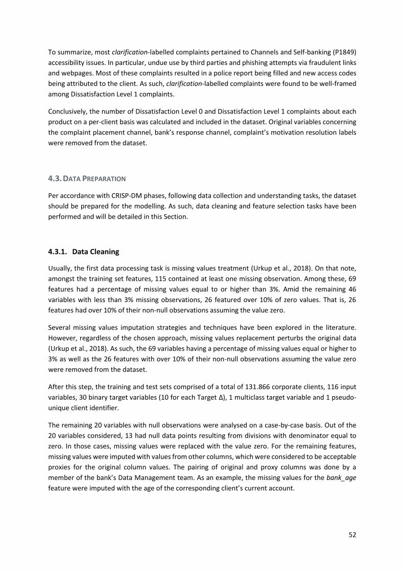
52
To summarize, most clarification-labelled complaints pertained to Channels and Self-banking (P1849)
accessibility issues. In particular, undue use by third parties and phishing attempts via fraudulent links
and webpages. Most of these complaints resulted in a police report being filled and new access codes
being attributed to the client. As such, clarification-labelled complaints were found to be well-framed
among Dissatisfaction Level 1 complaints.
Conclusively, the number of Dissatisfaction Level 0 and Dissatisfaction Level 1 complaints about each
product on a per-client basis was calculated and included in the dataset. Original variables concerning
the complaint placement channel, bank’s response channel, complaint’s motivation resolution labels
were removed from the dataset.
4.3. DATA PREPARATION
Per accordance with CRISP-DM phases, following data collection and understanding tasks, the dataset
should be prepared for the modelling. As such, data cleaning and feature selection tasks have been
performed and will be detailed in this Section.
4.3.1. Data Cleaning
Usually, the first data processing task is missing values treatment (Urkup et al., 2018). On that note,
amongst the training set features, 115 contained at least one missing observation. Among these, 69
features had a percentage of missing values equal to or higher than 3%. Amid the remaining 46
variables with less than 3% missing observations, 26 featured over 10% of zero values. That is, 26
features had over 10% of their non-null observations assuming the value zero.
Several missing values imputation strategies and techniques have been explored in the literature.
However, regardless of the chosen approach, missing values replacement perturbs the original data
(Urkup et al., 2018). As such, the 69 variables having a percentage of missing values equal or higher to
3% as well as the 26 features with over 10% of their non-null observations assuming the value zero
were removed from the dataset.
After this step, the training and test sets comprised of a total of 131.866 corporate clients, 116 input
variables, 30 binary target variables (10 for each Target Δ), 1 multiclass target variable and 1 pseudo-
unique client identifier.
The remaining 20 variables with null observations were analysed on a case-by-case basis. Out of the
20 variables considered, 13 had null data points resulting from divisions with denominator equal to
zero. In those cases, missing values were replaced with the value zero. For the remaining features,
missing values were imputed with values from other columns, which were considered to be acceptable
proxies for the original column values. The pairing of original and proxy columns was done by a
member of the bank’s Data Management team. As an example, the missing values for the bank_age
feature were imputed with the age of the corresponding client’s current account.

53
After having handled all null data points, the pseudo-unique identifier was removed from the training
set, and duplicated rows were deleted. In total, 131.854 client entries remained in the training and
test sets.
Next, columns with zero or almost zero variance (i.e., standard deviation strictly less than 0.001) have
been removed. Deleted features consisted of one financial indicator of the clients’ relationship with
the bank as well as all six variables relating to webpage activity for each of the six respective products.
At this stage, the training and test sets comprised of a total of 131.854 corporate clients, 109 input
variables, 30 binary target variables (10 for each Target Δ), and 1 multiclass target variable.
Next, a Pearson correlation analysis for the 99 numerical features in the training set was performed.
Among the 99 numerical variables considered, 22 were found to be highly correlated, and 9 were found
to be moderately correlated with other variables. The 0.5 threshold was considered for the absolute
value of Pearson correlation coefficients (Hinkle et al., 2003). The 31 variables presenting moderate to
high correlation coefficients were dropped. With this, the training and test sets totalled 131.854
corporate clients, 78 input variables, 30 binary target variables (10 for each Target Δ), and 1 multiclass
target variable.
Another implemented processing step was the one-hot encoding of categorical variables. In other
words, each categorical feature was mapped into a binary vector with length equal to C-1, with C being
the number of unique categories in the original categorical variable. This task was performed since the
machine learning models that will be trained during the modelling phase require all input features to
be numeric. One-hot encoding of categorical variables was implemented using the
pandas.get_dummies Python function. After one-hot encoding, the training and test sets totalled
131.854 corporate clients, 103 input variables, 30 binary target variables (10 for each Target Δ), and 1
multiclass target variable.
Lastly, a Standard Scaler was fitted to the training dataset. Standard Scaler is able to standardize the
dataset by removing the mean 𝜇 and scaling each feature 𝑥 to unit variance 𝜎, in accordance with
Equation 10.
𝑧𝑥 = 𝑥𝑖− 𝜇𝑥
𝜎𝑥 (10)
Hence, Standard Scaler is able to scale and centre each feature independently. This task was
undertaken since algorithms, like PCA, require the data to be standardized in order to avoid unit scaling
effects (Coste et al., 2005). Data standardization was done by applying Python’s
sklearn.preprocessing.StandardScaler() class. Once the scaler was fit to the training set, it was applied
to both the test and training sets. Further, in order to prevent information leakage between the
training and test dataset splits, standardization, Feature Selection and Extraction, modelling and
evaluation steps were assembled into a pipeline using sklearn’s pipeline.Pipeline class. This object
allows for a sequence of transformation steps to be applied together during cross-validation with a
fit() and transform() paradigm.

54
4.3.2. Feature Engineering
As previously mentioned, predictive algorithms tend to beneficiate from feature engineering. Since
not every feature is useful and considering the usage of models, such as the k-Nearest Neighbours,
which are sensitive to irrelevant features and high-dimensional feature spaces, as well as Logistic
Regression, which assumes little to no multicollinearity between input features, Feature Selection and
Extraction methods were employed. In this thesis, Principal Component Analysis (PCA) and Recursive
Feature Elimination (RFE) were considered for improving the models' performance.
Principal Component Analysis
Before Principal Components Analysis was carried out, the dataset’s adequacy was tested by the
Kaiser-Meyer-Olkin factor adequacy statistic, which was performed using the KMO function in R’ psych
package. This test returned a value of 0.5; the lowest value still acceptable for Principal Component
Analysis (Rea & Rea, 2016).
On this basis, PCA was implemented and executed on the correlation matrix using the prcomp R
function. As aforementioned, the original data was scaled and centred around 0. Thus, the PC loadings
can be interpreted as correlation coefficients between the Principal Components and the original input
features, hence facilitating PC interpretation (Coste et al., 2005).
For determining the number of Principal Components to retain, Kaiser’s criterion was employed. This
rule states one should retain only the Principal Components whose eigenvalue is larger than the mean
of all eigenvalues (Coste et al., 2005). In this context, where PCA was computed over the correlation
matrix, this is equivalent to selecting only the PCs with corresponding eigenvalues larger than 1. The
application of the Kaiser’s criterion returned the first 56 Principal Components, with a percentage of
the cumulative variance of approximately 70.38%.
Recursive Feature Elimination
Recursive Feature Elimination (RFE) was implemented as a wrapper feature selection method using
the sklearn.feature_selection.RFE class receiving as estimator each of the considered machine learning
algorithms.

55
5. EXPERIMENTAL STUDY
In this Chapter, experimental setup and Recommendation Systems’ performance results are presented
and discussed. Foremost, the evaluation strategies employed for evaluating Recommenders and FSE
methods performance are overviewed. Then, the evaluation metrics selected for performance
assessment are introduced and discussed. Further, performance results for both multi-output
regression and multiclass classification prediction approaches are discussed independently. At last, a
comparison between both prediction approached is carried out, followed by a more in-depth analysis
of the best overall model.
5.1. EVALUATION PROTOCOL
In order to assess Recommender performance, a 10-fold cross-validation evaluation strategy is used
(Urkup et al., 2018). As such, the training dataset is randomly divided into 10 equal-sized subsamples.
Out of these, one is taken as the holdout set. The learning model is then trained and tested 10 times,
using the holdout set for testing and the remaining folds for training.
The strategy employed for evaluating Feature Selection and Extraction methods was based on the
notion that the best FSE method is the one that most improves the learning model’s performance
(Urkup et al., 2018). Thus, improvement of model performance was taken as an indicator of FSE
methods performance.
5.2. EVALUATION METRICS
In this thesis, Recommender's performance is based on its ability to recommend relevant products to
the bank’s corporate clients. Evaluation metrics used in this thesis were chosen due to their
widespread usage in assessing the performance of Recommender Systems applied to financial
domains. Thus, to compare the learning models performances, F1 Measure, Precision, and Recall
metrics were selected as model evaluation criteria.
In the multi-output regression setting, the recommendation of the most suitable financial product
purchase for each corporate user 𝑢 corresponds to solving 𝑎𝑟𝑔𝑚𝑎𝑥(𝑣𝑢), where 𝑣𝑢 is the predicted
vector for a corporate client 𝑢. Thus, a recommendation is considered to be a True Positive (TP) when
the recommended product was indeed purchased by the client in the time span determined by the
target Δ considered. For example, if target Δ = 1 month, then product purchases up to 1 month from
the end of the base commercial cycle are considered.
Overall, True Positives (TP) measure the number of recommended financial products which were
indeed purchased by the corporate client. Recommendations that did not result in product purchases
are defined as False Positives (FP). True Negatives (TN) correspond to financial products that were
correctly not recommended, and False Negatives (FN) are products which were not recommended but
should have been, as they have been purchased by the client. On this basis, Precision measures the
Recommender’s correctness and can be defined by Equation 11.

56
𝑃𝑟𝑒𝑐𝑖𝑠𝑖𝑜𝑛 = 𝑇𝑃
𝑇𝑃 + 𝐹𝑃 (11)
High precision models minimize False Positives or the recommendation of products the user is not
interested in buying. In the specific application context of this thesis, Precision can, therefore, be linked
with customer satisfaction (Bogaert et al., 2019), as models having high Precision will not advise
account managers to suggest their corporate clients to purchase financial products which are not
relevant to them. As such, Precision can also be taken as a degree of confidence in the relevance of
the recommendation.
On the other hand, Recall (also known as sensitivity) measures Recommendation System’s coverage,
and it is given by Equation 12. Models with high Recall minimize False Negatives, that is, products the
users are interested in buying but are overlooked by the model. For the Recommender developed in
this thesis, Recall is closely related to profitability, as it is an indicator of the Recommender’s ability to
identify product purchasing opportunities.
𝑅𝑒𝑐𝑎𝑙𝑙 = 𝑇𝑃
𝑇𝑃 + 𝐹𝑁 (12)
Lastly, F1 Measure is calculated as the harmonic mean between Precision and Recall, as given by
Equation 13. The F1 Measure, combining Precision and Recall, was employed as a composite measure
for an overall model performance assessment.
𝐹1 𝑀𝑒𝑎𝑠𝑢𝑟𝑒 = 2 × 𝑃𝑟𝑒𝑐𝑖𝑠𝑖𝑜𝑛 × 𝑅𝑒𝑐𝑎𝑙𝑙
𝑃𝑟𝑒𝑐𝑖𝑠𝑖𝑜𝑛 + 𝑅𝑒𝑐𝑎𝑙𝑙 (13)
Evaluation metrics are assessed on both training and unseen test sets. While training set performance
is important for understanding the learning models' ability to model the data, performance evaluation
of unseen instances allows for an estimation of the Recommender’s generalization ability. A 10-fold
cross-validation was performed, reported metrics correspond to the average results obtained across
all 10 runs.
5.3. EXPERIMENTAL RESULTS AND DISCUSSION
This Section presents the results of the application of the aforementioned machine learning models
for both multi-output regression and multiclass classification prediction approaches. As previously
mentioned, hyperparameters for each learning algorithm have been tuned for both multi-output
regression and multiclass classification. Performance results for both prediction approaches are
discussed independently. Next, a comparison between them is carried out, followed by a more in-
depth analysis of the best overall model.

57
5.3.1. Experimental Results for Multi-Output Regression
Experimental results discussion starts by analysing the performance of the learning models in the
multi-output problem setting. In this prediction approach, the goal is to predict a 10-dimensional
vector denoting product purchase likelihood by corporate clients during the target commercial cycle.
As a first step, matrix sparsity was calculated for each of the three target Δs considered. Sparsity for a
given matrix 𝑀 is given by Equation 14. Matrix sparsity results are shown in Table 9.
% 𝑆𝑝𝑎𝑟𝑠𝑖𝑡𝑦 = 100 × (1 − # non−zero elements(𝑀)
# elements(𝑀)) (14)
Table 9 - Sparsity percentage in multi-output target User-Item matrix for Δ1, Δ2, and Δ3
Sparsity of the Training Target Binary Matrix
Multi-Output Target Δ1 99.46%
Multi-Output Target Δ2 99.05%
Multi-Output Target Δ3 98.81%
According to Table 9, as more months are considered for the product purchase registry, the number
of positions assigned the value 1 on the binary target vectors increases. Hence, the sparsity of the User-
Item target matrix decreases as the target’s Δ increases. Thus, it is expected the algorithms perform
better for Multi-Output Target Δ3, then for Multi-Output Target Δ2, or Multi-Output Target Δ1.
This assumption was validated by training each multi-output learning model on the training set for
each of the three multi-output target Δs. F1 Measure, Precision, and Recall were evaluated on the
training and test sets. Figure 16 shows the 10-fold averaged F1, Precision, and Recall values per multi-
output learning algorithm, configured for optimally tuned hyperparameters, for each multi-output
target Δs.

58
Figure 16 - Multi-output models’ performance for different target Δs
Tuned models’ performance is evaluated on average F1 Measure, Precision,
and Recall over 10-fold cross-validation for both training and test sets.
Overall, the hypothesis that learning models would perform better for less sparse User-Item matrixes
has been verified. On the training data, the average F1 Measure over target Δ3 is higher than F1 over
target Δ1 for all the considered learning models. Moreover, it is higher or comparable to the averaged
F1 measured over target Δ2. Furthermore, on unseen data samples, F1 measured on data considering
all three target commercial cycle months is, for all considered models, strictly higher than F1 over
target Δ2 or target Δ1.
Regarding F1 measured on the training data, both Logistic Regression and Random Forest do not
register an increased performance when considering all three months rather than just the first two
months of the target commercial cycle. Conversely, the Feed-Forward Neural Networks algorithm

59
presents the most significant improvement in F1 over target Δ3 when compared to target Δ2. For the
same conditions, k-Nearest Neighbours algorithm shows only a slight improvement in performance.
Notwithstanding, for unseen data points, all learning models achieve a higher F1 and Recall
performance on the dataset considering all three months. Regarding the Precision score, 3 out of the
4 learning models considered display better or akin results for target Δ1 when compared with target
Δ3. Upon further analysis, on account of the low number of registered product purchases during only
the first month of the target commercial cycle, the learning models were producing a proportionally
small number of financial product recommendations. Thus, the number of generated False Positive
recommendations for target Δ1 was smaller than the one produced over target Δ3, leading to slightly
better Precision score results.
To better understand the algorithms’ generalization ability, the difference between training and test
F1 Measures was taken as quantification of overfitting. A graphical display of the obtained results can
be seen in Figure 17.
Figure 17 - Multi-output models’ overfitting for different target Δs
Average difference between 10-fold cross-validated F1 score measured
on the training and test sets for the tuned multi-output learning models
applied to the different target Δs.
From the inspection of Figure 17, Random Forest models present the highest overfitting. This condition
could be partially explained by the hyperparameters selected during cross-validated grid search. As
aforementioned, individual Decision Trees are prone to overfitting. In Random Forest algorithms, this
tendency is mitigated through training the base learners with bootstrap samples of the training data
and the introduction of randomness in the subset of features considered to decide node split. Apart
from these two mechanisms, tree pruning can also be used to mitigate the algorithm’s proneness to
overfit noisy or atypical data. However, in this thesis, as part of the best hyperparameters
configuration, cross-validated grid search identified that base learners grown to full size (i.e., without
pruning) produced better cross-validated results than alternative min_samples_leaf hyperparameter
settings.

60
On the other hand, kNN and Logistic Regression present negligible overfitting. For k-Nearest
Neighbours algorithms, this is mostly due to the wide number of neighbours considered in each data
point’s neighbourhood. Feed-Forward Neural Networks have slightly higher overfitting, although this
has already been mitigated by the application of regularization techniques, namely Early Stopping and
dropout. Overall, the best multi-output learning models’ performance was considered to be achieved
with target Δ3. Hence, such performance was, from this point onwards, considered as the baseline to
assess the impact of the application of FSE methods.
Next, experimental results for the impact of applying FSE techniques are presented. As previously
mentioned, the performance of Feature Selection and Extraction methods was taken as the
improvement they provide to a base model’s performance. As such, grid-searched tuned multi-output
learning models’ performance with target Δ3 was considered as a baseline for comparison.
Experimental results for baseline learning models, and RFE and PCA learning model architectures are
reported in Figure 18.
(a)
(b)
(c)
(d)
Figure 18 - Performance results for multi-output models’ architectures Average 10-fold cross-validated F1 Measure, Precision, and Recall for both
training and test sets evaluated on Multi-Output Target Δ3, trained on Principal
Components and with RFE feature selection method for multi-output (a) Feed-
Forward Neural Networks, (b) k-Nearest Neighbours, (c) Logistic Regression,
and (d) Random Forests
From Figure 18, it appears that Feature Selection and Extraction (FSE) methods have a significant
positive impact on Feed-Forward Neural Networks performance. FNN, in combination with Recursive

61
Feature Elimination (RFE), results in the higher averaged F1 score measured on the test set. This model
surpasses the second runner-up by a large margin, achieving almost double F1 performance than the
combination of Feed-Forward Neural Networks and Principal Component Analysis. The FNN baseline
presents the worst performance on the test set for all considered evaluation metrics, thus supporting
the hypothesis that Feature Selection and Extraction methods can allow for a significant improvement
in Recommender performance.
For k-Nearest Neighbours, albeit not as significantly impacting Recommender performance, RFE
contributes to improving both F1, Precision as well as Recall values on the test set. Comparatively, the
combination of Principal Components with kNN learning model produced the worst performance,
being surpassed by the baseline architecture in all metrics evaluated on the test set.
For multi-output Logistic Regression, on the other hand, the combination of the learning model with
Principal Component Analysis (PCA) slightly outperforms both the baseline and RFE alternative models.
These results are in agreement with Logistic Regression’s assumption of no multicollinearity between
input features.
Lastly, RFE methods did not prove useful in increasing Random Forest model performance. Moreover,
the application of dimensionality reduction methods, such as PCA, result in a significant decrease in
Recommender performance. Upon analysis, due to Random Forest models having built-in embedded
feature selection mechanisms, it was found that these models do not benefit from previous feature
selection and extraction efforts.
With respect to the multi-output learning models’ generalization ability, the difference between 10-
fold averaged F1 score evaluated on the training and test sets was taken as an indicator of the models’
tendency to overfit the data. As such, algorithms with low F1 overfitting scores are considered to
generalize better, and, reciprocally, high F1 overfitting values are associated with architectures lacking
generalization ability.
Figure 19 - F1-based overfitting scores for the different multi-output architectures
Average difference between 10-fold cross-validated F1 score measured on the training and
test sets for the tuned multi-output learning model applied to Target Δ3 (Base), trained on
Principal Components (PCA) and combined with Recursive Feature Elimination (RFE).

62
Regarding the models’ overfitting, as shown in Figure 19, for both FNN and kNN Recommenders, the
application of PCA increases the models’ tendency to overfit the training data. In the case of Feed-
Forward Neural Networks, RFE technique has a very positive impact on the algorithm’s generalization
ability, reducing F1 Measure overfitting by 10% when compared to the baseline approach. For Logistic
Regression, FSE methods contribute to reducing the difference in F1 training and testing scores
drastically. At last, for Random Forest models, PCA appears to reduce the overfitting, albeit in
detriment of algorithm performance.
In this stage, the best performing model architecture for each multi-output learning model was taken
for comparison. Considering all three performance metrics evaluated on the test set, the best
architecture for multi-output learning models was considered to be Feed-Forward Neural Networks
combined with Recursive Feature Elimination, achieving an F1 of 28.92%, a Precision score of 23.00%
and a Recall of 38.92%. RFE wrapper feature selection with k-Nearest Neighbours algorithm,
presenting an F1, Precision, and Recall of 27.70%, 24.21%, and 32.37%, respectively, was found to be
the best kNN learning model architecture. For Logistic Regression, a combination with PCA produced
the highest F1 score of 26.52%, with corresponding Precision and Recall of 19.34% and 42.18%. Lastly,
baseline Random Forest over target Δ3 appeared as the best performing model with an F1, Precision,
and Recall of 30.24%, 20.56%, and 57.21%.
Overall, considering the best multi-output regression model architectures, Random Forest appears to
be the best performing algorithm for the F1 Measure, closely trailed by RFE+FNN, RFE+KNN, and
PCA+Logistic Regression. The test set averaged performance results for the best multi-output model
architectures are shown in Figure 20.
Figure 20 - F1, Precision and Recall for the best performing multi-output architectures
For the best performing multi-output regression model architectures, F1 measured on the test set
ranged from 26.51% to 30.24%. Corresponding values of Precision and Recall range from 19.34% to
24.21%, and from 32.37% to 57.21%, respectively.

63
Figure 21 reports the Standard Deviation for 10-fold cross-validated F1 scores on the test set. In the
boxplots displayed on Figure 21, the central line in each box corresponds to the median, the cross
marker corresponds to the mean F1 value, the upper and lower box limits are, respectively, the first
and third quartiles, and the whiskers extend to the maximum and minimum F1 measurements.
Further, Standard Deviation values for 10-fold generalization F1 scores are presented for each learning
model.
Figure 21 - Boxplots for the best performing multi-output architectures
Standard Deviation ranges from 0.018 to 0.046. Among the considered models, RFE+FNN architecture
produces the most stable results, with a Standard Deviation of 1.8%, while F1 scores for Random Forest
over target Δ3 present the highest variation, reaching a Standard Deviation value of 4.6%.
5.3.2. Experimental Results for Multiclass Classification
In this subsection, performance results for learning models applied to a multiclass classification setting
are discussed. First, a performance comparison for multiclass learning models and architectures,
combining them with Recursive Feature Elimination and Principal Components Analysis techniques, is
provided. For this purpose, the performance of 10-fold cross-validated grid-searched tuned multiclass
models was taken as a baseline, and improvements on the evaluation metrics were considered to be
indicators of FSE methods performance. Experimental results for the impact of applying RFE and PCA
to multiclass learning models are reported in Figure 22.

64
(a)
(b)
(c)
(d)
Figure 22 - Performance results for multiclass models’ architectures
Average 10-fold cross-validated F1 Measure, Precision, and Recall for both
training and test sets evaluated on the processed dataset, trained on
Principal Components and with RFE feature selection method for multiclass
(a) Feed-Forward Neural Networks, (b) k-Nearest Neighbours, (c) Logistic
Regression, and (d) Random Forests
From the analysis of Figure 22, it can be seen that all four baseline multiclass learners present a
comparable 10-fold averaged F1 performance on the test set. This metric, when evaluated on unseen
samples, ranged from 44.44% to 52.08%, with Random Forest achieving the highest performance,
followed closely by k-Nearest Neighbours with an F1 score of 51.94%, and Feed-Forward Neural
Networks, with 51.04% F1 score. Logistic Regression had the worst performance resulting in an F1
value of 44.44%.
RFE and PCA applied to multiclass learning models produced qualitatively comparable results to FSE
methods application in the multi-output setting. More precisely, similarly to multi-output FNN, also
for multiclass learners, the application of Feature Selection and Extraction (FSE) methods appears to
have a positive impact on multiclass Feed-Forward Neural Networks’ performance. The combination
of RFE with FNN emerges as the best performing architecture, bettering the baseline’s F1 score,
Precision, and Recall by 30 percentage points each. Principal Components, on the other hand, only
introduce a slight improvement over the baseline’s performance, increasing all evaluation metrics
values by around 6 percentage points.
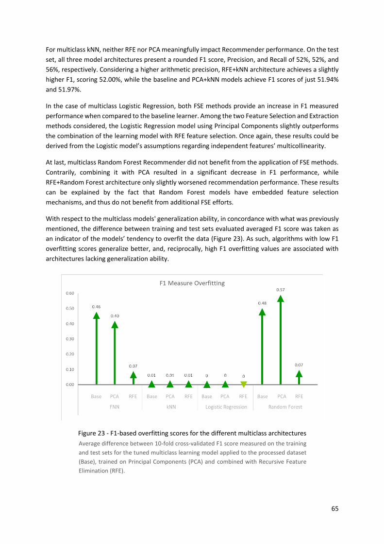
65
For multiclass kNN, neither RFE nor PCA meaningfully impact Recommender performance. On the test
set, all three model architectures present a rounded F1 score, Precision, and Recall of 52%, 52%, and
56%, respectively. Considering a higher arithmetic precision, RFE+kNN architecture achieves a slightly
higher F1, scoring 52.00%, while the baseline and PCA+kNN models achieve F1 scores of just 51.94%
and 51.97%.
In the case of multiclass Logistic Regression, both FSE methods provide an increase in F1 measured
performance when compared to the baseline learner. Among the two Feature Selection and Extraction
methods considered, the Logistic Regression model using Principal Components slightly outperforms
the combination of the learning model with RFE feature selection. Once again, these results could be
derived from the Logistic model’s assumptions regarding independent features’ multicollinearity.
At last, multiclass Random Forest Recommender did not benefit from the application of FSE methods.
Contrarily, combining it with PCA resulted in a significant decrease in F1 performance, while
RFE+Random Forest architecture only slightly worsened recommendation performance. These results
can be explained by the fact that Random Forest models have embedded feature selection
mechanisms, and thus do not benefit from additional FSE efforts.
With respect to the multiclass models' generalization ability, in concordance with what was previously
mentioned, the difference between training and test sets evaluated averaged F1 score was taken as
an indicator of the models’ tendency to overfit the data (Figure 23). As such, algorithms with low F1
overfitting scores generalize better, and, reciprocally, high F1 overfitting values are associated with
architectures lacking generalization ability.
Figure 23 - F1-based overfitting scores for the different multiclass architectures
Average difference between 10-fold cross-validated F1 score measured on the training
and test sets for the tuned multiclass learning model applied to the processed dataset
(Base), trained on Principal Components (PCA) and combined with Recursive Feature
Elimination (RFE).

66
As reported in Figure 23, for FNN, Logistic Regression, and Random Forest learning models, the
application of Recursive Feature Elimination positively impacts the generalization ability. For FNN and
Random Forest, in particular, RFE architectures reduce F1 Measure overfitting in 30 to 40 percentage
points. When compared to the baseline learner, combining PCA with FNN reduces F1 overfitting.
However, the opposite effect is found for Random Forest classifiers, where Principal Components
increase model overfitting. Overall, kNN and Logistic Regression models present exceedingly low F1
overfitting. Architectures combining either FNN or Random Forest models with RFE achieve relatively
good results, with F1 train-test discrepancies of just 7%. Conversely, baseline and PCA architectures of
FNN and Random Forest models present high order generalization errors, possibly requiring further
regularization and parameter tuning efforts.
In this stage, the best performing multiclass model architecture was taken for comparison. Considering
the performance metrics evaluated on the test set, Feed-Forward Neural Networks combined with
Recursive Feature Elimination was found as the best FNN model architecture, achieving an F1 of
83.16%, a Precision score of 84.34% and a Recall of 85.29%. RFE wrapper feature selection with k-
Nearest Neighbours algorithm presenting an F1, Precision, and Recall of 52.00%, 52.36%, and 55.62%,
respectively, was considered to be the best kNN learning model architecture. Even though its
performance only surpassed alternative kNN-based Recommender configuration by a very thin margin,
the application of RFE reduced the dataset’s feature space, thus decreasing computational runtime.
For Logistic Regression, a combination with PCA produced the highest F1 score of 47.73%, with
corresponding Precision and Recall of 48.21% and 48.33%. Lastly, the baseline configuration of
multiclass Random Forests appeared as the best performing model with an F1, Precision, and Recall of
52.08%, 55.87%, and 57.34%.
Overall, among the best multiclass architectures for each learning model, the combination of RFE with
FNN emerges as the best performing algorithm for all considered test set evaluation metrics. The
remaining algorithms achieved similar F1, Precision and Recall scores, with Random Forest appearing
as the second-best model, closely trailed by RFE+kNN, and PCA+Logistic Regression. The test set
averaged performance results for the best multiclass models are shown in Figure 24.
Figure 24 - F1, Precision and Recall for the best performing multiclass architectures

67
For the best performing multiclass model architectures, F1 measured on the test set ranged from
47.73% to 83.16%. Corresponding values of Precision and Recall range from 48.21% to 84.34%, and
from 48.33% to 85.29%, respectively.
Figure 25 reports the Standard Deviation for 10-fold cross-validated F1 scores on the test set. Once
again, for the boxplots displayed in Figure 25, the central line in each box corresponds to the median,
the cross marker to the mean F1 value, the upper and lower box limits are, respectively, the first and
third quartiles, and the whiskers extend to the maximum and minimum F1 measurements.
Figure 25 - Boxplots for the best performing multiclass architectures
From the interpretation of Figure 25, Standard Deviation ranges from 0.001 to 0.009. Among the
considered models, RFE+FNN architecture produces the most stable results, with a Standard Deviation
of 0.1%, while PCA+Logistic Regression’s F1 scores present the highest variation, reporting a slightly
higher Standard Deviation value of 0.9%. Generally, all Standard Deviation values are low, implying
that the multiclass model architectures considered produce stable results.
5.3.3. Comparison Between Prediction Approaches
In this subsection, results for the best architectures for both multi-output regression and multiclass
classification approaches will be analysed and compared. A discussion vising to address the research
questions formulated during the Business Understanding project phase will also be carried out. Figure
26 summarizes test set performance for the best architectures found for the two prediction
approaches considered.

68
Figure 26 - Comparison of the best performing multi-output and multiclass architectures
Average F1, Precision, and Recall metrics, evaluated on the test set, for the best performing model
architectures of both multi-output and multiclass prediction approaches.
As reported in Figure 26, multiclass learners generally yield better results when compared to multi-
output regression-based architectures. Multi-output learning models appear to have poor
performance, with PCA combined with Logistic Regression performing worst from both F1 and
Precision scores, and multi-output RFE+kNN presenting the lowest Recall among the considered
architectures. Multiclass Feed-Forward Neural Networks, in combination with Recursive Feature
Elimination, appears as the best performing algorithm for all evaluation metrics considered, followed
by multiclass Random Forests, and multiclass kNN in combination with RFE feature selection.
Furthermore, a detailed analysis of the obtained results allowed the following remarks. First, the
worst-performing algorithms were observed to be characterized by higher Recall values and rather low
Precision scores. Practical implications of models having high Recall and low Precision are that they
succeed in recommending the majority of relevant items, albeit in detriment of also recommending a
large number of irrelevant instances. In short, such models have a small number of False Negative
recommendations due to their high Recall rate but produce a large number of False Positives due to
their low Precision. One might argue that such models provide more complete recommendations,
since producing a small number of False Negative recommendations leads to most relevant items being
recommended. However, when a high Recall rate is combined with low Precision scores, this results in
a large number of False Positive recommendations being generated.
In the context of this project, acting upon such recommendation will lead account managers to suggest
financial products the users are not interested in, thus decreasing overall customer satisfaction.
Therefore, considered multi-output regression models, which are characterized by higher Recall rates
and lower Precision values, favour the harness of sales opportunities, and hence the increase of
customer value and corporate profitability, over customer satisfaction.
Alternatively, models having high Precision but low Recall rates will focus on recommending truly
relevant items (i.e., minimizing the number of False Positives) in detriment of neglecting to
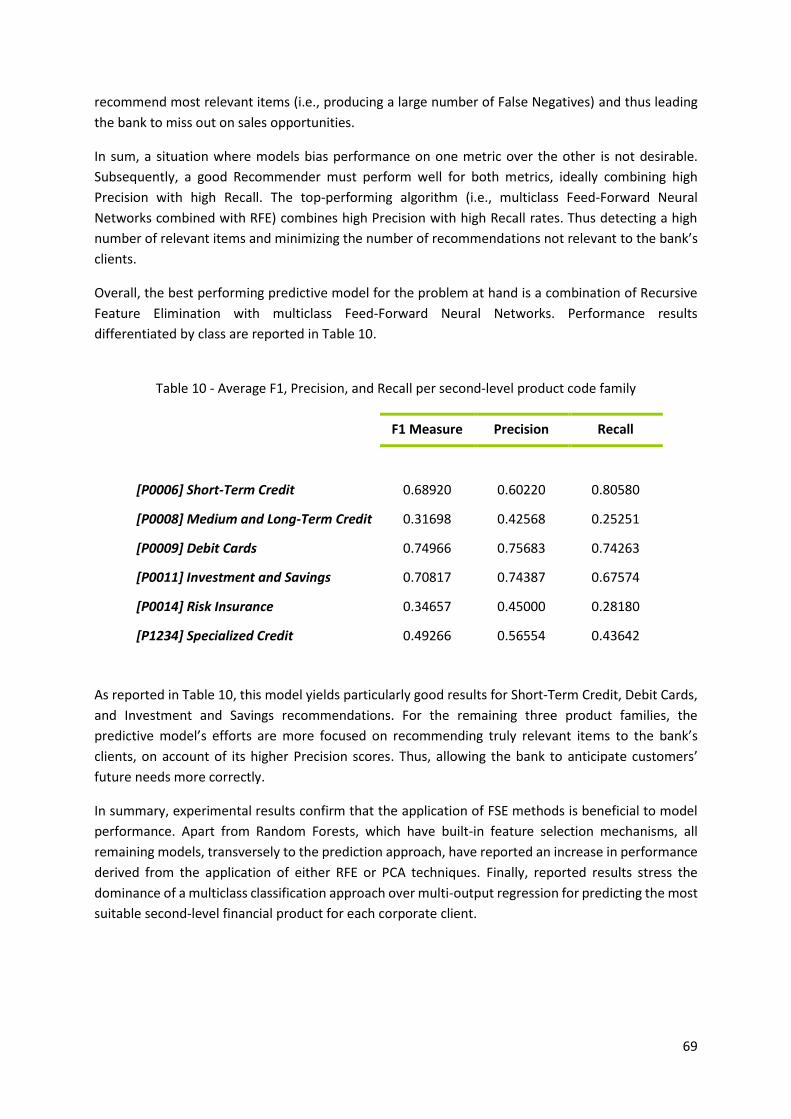
69
recommend most relevant items (i.e., producing a large number of False Negatives) and thus leading
the bank to miss out on sales opportunities.
In sum, a situation where models bias performance on one metric over the other is not desirable.
Subsequently, a good Recommender must perform well for both metrics, ideally combining high
Precision with high Recall. The top-performing algorithm (i.e., multiclass Feed-Forward Neural
Networks combined with RFE) combines high Precision with high Recall rates. Thus detecting a high
number of relevant items and minimizing the number of recommendations not relevant to the bank’s
clients.
Overall, the best performing predictive model for the problem at hand is a combination of Recursive
Feature Elimination with multiclass Feed-Forward Neural Networks. Performance results
differentiated by class are reported in Table 10.
Table 10 - Average F1, Precision, and Recall per second-level product code family
F1 Measure Precision Recall
[P0006] Short-Term Credit 0.68920 0.60220 0.80580
[P0008] Medium and Long-Term Credit 0.31698 0.42568 0.25251
[P0009] Debit Cards 0.74966 0.75683 0.74263
[P0011] Investment and Savings 0.70817 0.74387 0.67574
[P0014] Risk Insurance 0.34657 0.45000 0.28180
[P1234] Specialized Credit 0.49266 0.56554 0.43642
As reported in Table 10, this model yields particularly good results for Short-Term Credit, Debit Cards,
and Investment and Savings recommendations. For the remaining three product families, the
predictive model’s efforts are more focused on recommending truly relevant items to the bank’s
clients, on account of its higher Precision scores. Thus, allowing the bank to anticipate customers’
future needs more correctly.
In summary, experimental results confirm that the application of FSE methods is beneficial to model
performance. Apart from Random Forests, which have built-in feature selection mechanisms, all
remaining models, transversely to the prediction approach, have reported an increase in performance
derived from the application of either RFE or PCA techniques. Finally, reported results stress the
dominance of a multiclass classification approach over multi-output regression for predicting the most
suitable second-level financial product for each corporate client.

70
6. DEPLOYMENT
After experimental results’ evaluation and assertion of the fulfilment of the proposed business
objectives, the project results were organized and reported to the Analytics and Models team’s
liaisons. Furthermore, although production, monitoring, and maintenance stages were out of scope
for this thesis, preliminary deployment tasks have been carried out. Ergo, this Chapter provides an
outline of preliminary deployment tasks, including a commercial viability assessment for the proposed
Recommender through ex-post backtesting, as well as an outline of the deployment plan.
6.1. ASSESSMENT OF COMMERCIAL VIABILITY
To emphasize the value of the proposed Recommender in marketing processes, a backtesting for the
second commercial cycle of 2020 was conducted. Backtesting the proposed model allows for an
evaluation of how it would have performed ex-post. The main purpose of this analysis is to provide an
assessment of the commercial viability of the proposed Recommender. That is, to stress the model’s
aptitude to advise account managers on which product would better suit their clients’ needs as well
as to explore potential marketing opportunities arising from produced recommendations.
Table 11 summarizes the mapping between predicted and observed first sales of a second-level
product to corporate clients in the second commercial cycle of 2020 (from April 1, 2020, to June 30,
2020). The required set of features that informed the results reported in Table 11 was collected at the
end of the first commercial cycle of 2020. On this basis, the best performing model was used to predict
the first second-level financial product purchase for each corporate client. At the end of the second
commercial cycle of 2020, observed first product sales for each client were retrieved.
Table 11 - Mapping between predicted and observed first sales of second-level products
From the analysis of Table 11, one can argue that 85% of first Short-Term Credit product sales were
correctly predicted by the model. Additionally, 71% and 72% of Debit Card purchases and Investment
and Savings product sales, respectively, were also correctly forecasted. With regard to Medium and
Long-Term Credit products, only 38% of the first sales were properly identified as such. The majority
was incorrectly predicted as Short-Term Credit sales. Similar scenarios were found for Risk Insurance
and Specialized Credit products.
Upon further analysis, three reasons were appointed for the obtained results. First, Short-Term Credit
products feature the highest first product acquisition rate among all considered second-level product
classes. As such, the proposed Recommender accompanies this acquisition rates imbalance by biasing
predictions for Short-Term Credit products.
Secondly, the reported results could be impaired by the ambiguity associated with implicit negative
instances. That is, corporate clients may not have purchased the predicted products not because they
have no interest in acquiring them, but because they do not know about them. Account managers will

71
play a crucial role in mitigating the impact of ambiguous negative instances, as they will contact the
corporate clients to present and suggest to them the predicted product.
Lastly, Table 11 only maps observed and predicted first sales of second-level financial products.
Building on the notion that clients may not be aware of the product the Recommender predicted for
them, corporate clients may have first acquired another financial product and only subsequently
bought the second-level product predicted by the Recommender. To further develop this notion,
registered product purchases throughout the commercial cycle have been analysed in Figure 27.
Figure 27 - Percentage of registered second-level product sales per likelihood percentile
Proportion of observed sales per purchase likelihood percentile for Short-Term Credit, Medium
and Long-Term Credit, Debit Cards, Investment and Savings, Risk Insurance, Specialized Credit

72
In Figure 27, the likelihood scores predicted by the Recommendation System for each product family
were divided into percentiles. A percentile is a statistical measure indicating the value below which a
certain percentage of observations can be found. That is, the nth percentile is the value below which
n% of all observations are found.
According to Figure 27, the Recommender performance per percentile shows very encouraging results.
For Medium and Long-Term Credit products, 58% of recorded sales during the second commercial
cycle of 2020 occur amid the 10th percentile of corporate users predicted to acquire products of this
class. For Debit Cards, this percentage increases to 68%. While for Specialized Credit products, 80% of
product sales can be found within the 10th percentile.
For the remaining product families, this percentage is slightly lower. However, considering the 20%
corporate clients predicted to most likely acquire each product class, 48% of Short-Term Credit sales,
53% of Investment and Savings product purchases, and 65% of Risk Insurance subscriptions are
accounted for.
6.2. DEPLOYMENT PLAN
In preparation for putting the model into production, data collection scripts were revised and altered
to allow them to be parameterized more easily and, thus, more seamlessly integrated into marketing
applications and processes. Additionally, data preparation and processing, as well as feature selection
and modelling tasks, have been automated and integrated into a machine learning pipeline, using the
pipeline.Pipeline class of sklearn.
Then, among the currently active marketing campaigns directed at corporate clients, the set of
campaigns marketing the purchase of financial products belonging to the specified second-level
product families have been identified as marketing campaigns potentially benefitting from the
integration of the proposed system’s recommendations.
Lastly, the main lines for the deployment of the Recommender into the lead generation framework for
these campaigns were delineated. For the first commercial cycle upon model deployment and
integration with lead generation applications, to further assess the Recommender’s impact on sales
and marketing processes, an isolated group of corporate clients will be defined as the control group
for each campaign. While for remaining corporate clients, the account managers will receive the
Recommendation System’s suggestions, for the control group, such recommendations will not be
provided. Therefore, with the establishment of the control group as a baseline for comparison, it will
be possible to more accurately estimate the Recommender’s influence and impact on commercial Key
Performance Indicators (KPIs), such as the marketing contacts conversion rate.

73
7. CONCLUSIONS
In this thesis, the challenge was to investigate how Recommender Systems can help automate the
choice of the most suitable financial product for a bank’s corporate customers, aiming to foresee their
future needs and requirements. The applied research in this thesis was based on a case study using an
anonymized real-world dataset provided by a Portuguese private commercial bank. Independent
variables featured in the provided dataset pertained to financial product ownership, socioeconomic
context attributes, behavioural information, and financial indicators of the customers’ relationship
with the bank.
While retail banking serves individual customers, corporate banking addresses clients belonging to the
corporate sector, namely institutions, companies, businesses, municipalities, and condominiums. For
this thesis’ case study, and following the business model’s constraints and requirements, the
Recommender’s client base was composed by the bank’s active, segmented, and consenting corporate
customers.
Two distinctive approaches to the recommendation task at hand were investigated: Multi-Output
Regression, and Multiclass Classification. The first approach considered a vector of item ratings,
denoting item purchase likelihood, as the prediction target. In turn, the second approach aimed to
predict the product that was most likely to be bought from the range of available second-level financial
products.
The CRISP-DM research methodology was adopted for this thesis’ data mining project development.
Business Understanding tasks, namely research on the bank’s business model, as well as business and
project requirements elicitation, were carried out in order to formulate this thesis’ problem definition.
During the Data Understanding phase, a preliminary understanding of the influence of independent
variables and main factors prompting corporate clients to purchase the bank’s financial products was
formulated. To do so, an exploratory data analysis was conducted, with the goal of generating initial
insights into the prediction problem, and the relationship between predictors and dependent
variables. Subsequently, Data Preparation tasks were implemented for preparing the dataset for
posterior Modelling and Evaluation phases.
According to the features provided in the data, four Collaborative-Demographic Hybrid
Recommenders, based on established supervised machine learning methods, were implemented and
evaluated. k-Nearest Neighbours, Random Forest, Logistic Regression and Feed-Forward Neural
Networks supervised machine learning algorithms and Recursive Feature Elimination, and Principal
Components Analysis FSE methods were selected, according to the surveyed literature on
Recommender Systems applied to financial domains.
Following Recommenders’ Modelling phase, a comparison of the application of Recommenders in each
of the two considered prediction approaches was performed. Additionally, an assessment of Feature
Selection and Extraction methods’ impact on Recommendation Systems’ performance was conducted.
Recommenders’ performance was assessed over three established metrics in Recommender
literature. As such, F1 Measure, Precision, and Recall were taken as model evaluation criteria.
Hyperparameter tuning efforts relied on 5-fold cross-validated grid search optimization while
Recommenders’ performance assessment employed a 10-fold cross-validation strategy, with reported
results corresponding to the averaged metrics across cross-validation folds.

74
In terms of feature engineering efforts, RFE and PCA methods were included in combination with the
base Recommenders. Thus, improvements to recommendation performance were considered as
indicators of FSE methods’ performance.
According to obtained experimental results, it was shown that Multiclass Classification Recommenders
outperform most of the remaining Multi-Output Regression-based architectures for all evaluation
metrics.
In general, Multi-Output Recommenders performed poorly for the task of determining the most
suitable financial product for each corporate client. For this prediction approach, Random Forest was
the top-performing algorithm, with an average cross-validated F1 Measure of 30.24%, and Precision
and Recall of 20.56% and 57.21%, respectively.
Multiclass Recommenders performed comparatively better for the prediction task at hand. Based on
the reported results, Multiclass Feed-Forward Neural Networks, in combination with Recursive Feature
Elimination, yielded the best results for all performance metrics considered, presenting an average
cross-validated F1 Measure, Precision, and Recall of 83.16%, 84.34%, and 85.29%.
Also, in terms of the predicted results’ stability, multiclass approaches established their prevalence
over Multi-Output Regression Recommenders. With regard to the Standard Deviation of 10-fold cross-
validated F1 measures, multi-output models presented higher variations, ranging from 0.18 to 0.046.
Whilst, multiclass architectures produced more stable results, with Standard Deviation values ranging
from 0.001 to 0.009. For both approaches, Feed-Forward Neural Networks with RFE achieved the
lowest variation.
In conclusion, multiclass Recommenders were shown to be more performant at predicting the most
suitable financial product for each of the bank’s corporate clients. Additionally, the assumption that
Recommenders’ performance could benefit from the application of FSE methods found support on the
experimental results reported as, apart from Random Forests, which have built-in feature selection
mechanisms, all remaining models, transversely to the prediction approach, have reported an increase
in performance derived from the application of either RFE or PCA techniques.
Ultimately, produced recommendations will be integrated into marketing and sales leads generation
processes and be passed onto the respective account managers. Therefore, the proposed
Recommender will allow to provide added value to account managers’ recommendations and more
accurately target marketing campaigns, anticipating clients’ needs and reducing unwanted client
contacts, leading to increased customer satisfaction and value.

75
7.1. LIMITATIONS
The applied research in this thesis was based on a case study using a real-world dataset provided by a
Portuguese private commercial bank. The provided dataset was not only subject to business model
restrictions but also subject to data confidentiality requirements. As part of the case study’s
constraints, the developed Recommender System was required to exclusively base its prediction upon
the data provided by the bank. Additionally, the Recommender’s independent variables were required
to solely pertain to the base commercial cycle. As a consequence, only the available information
regarding the social-economic profile and customers’ relationship with the bank could be leveraged.
Otherwise, other relevant information, such as social media information or historical data for each
corporate client since they became bank customers, could be leveraged to enhance the
recommendation process.
In addition, the provided dataset did not include product content information. Thus, strategies
comprising the setup and exploration of Content-Based approaches were rendered impracticable.
Content-Based Recommenders are premised on profiles of the users’ preferences, thus requiring
detailed product information and characteristics. Despite their unpredictable performance in financial
domains, Content-Based Recommenders are, nonetheless, an interesting research line. Moreover,
such systems could as well be combined into Hybrid Recommenders, alongside Collaborative and
Demographic Filtering approaches.
7.2. FUTURE WORK
Future improvements would firstly focus on addressing the identified limitations in order to mitigate
their impact and remove noted impediments. Additionally, three lines of research are suggested for
further investigation.
First, the conduction of a real-life experiment in which the Recommender System proposed is
integrated into the bank’s marketing leads generation process. This experiment should feature a set
of corporate clients, termed control group, for whom the generated leads will not incorporate the
Recommendation System’s predictions. In this way, given that the experiment surveys a sufficiently
long testing period, it will be possible to confirm the proposed model’s contributions and assess its
real-world applicability, beyond ex-post and offline evaluation metrics.
The second direction for future research pertains to the incorporation of different types and sources
of information. Project improvements could be gained from considering indicators of commercial
activity sectors, financial market, and macroeconomic trends influencing corporate clients’ purchasing
behaviour.
The third future research line may regard the identification of social and commercial relationships
between the bank’s corporate and private customers, leading to the construction of a financial social
network. As supported by Recommender literature, Social Network Analysis (SNA) encompasses a
promising research direction, reflecting the effects of social ties and economic relationships on
consumer behaviour.

76
8. BIBLIOGRAPHY
Abdollahpouri, H., & Abdollahpouri, A. (2013). An approach for personalization of banking services in
multi-channel environment using memory-based collaborative filtering. The 5th Conference on
Information and Knowledge Technology, 208-213.
Adomavicius, G., & Tuzhilin, A. (2005). Toward the next generation of recommender systems: a survey
of the state-of-the-art and possible extensions. IEEE Transactions on Knowledge and Data
Engineering, 17, 734-749.
Ahmad, A., & Khan, S.S. (2019). Survey of State-of-the-Art Mixed Data Clustering Algorithms. IEEE
Access, 7, 31883-31902.
Azevedo, A., & Santos, M. (2008). KDD, SEMMA and CRISP-DM: a parallel overview. IADIS European
Conf. Data Mining.
Barranco, M. J., Noguera, J. M., Castro, J., & Martínez, L. (2012). A context-aware mobile recommender
system based on location and trajectory. Advances in Intelligent Systems and Computing, 153–
162. Springer Berlin Heidelberg.
Bobadilla, J., Ortega, F., Hernando, A., & Gutiérrez, A. (2013). Recommender systems survey.
Knowledge-Based Systems, 46, 109-132.
Bogaert, M., Lootens, J., Van den Poel, D., & Ballings, M. (2019). Evaluating multi-label classifiers and
recommender systems in the financial service sector. European Journal of Operational Research,
279, 620-634.
Brittain, J., Cendon, M., Nizzi, J., & Pleis, J. (2018). Data scientist’s analysis toolbox: Comparison of
Python, R, and SAS Performance. SMU Data Science Review, 1, 7.
Brown, I., & Mues, C. (2012). An experimental comparison of classification algorithms for imbalanced
credit scoring data sets. Expert Systems with Applications, 39, 3446-3453.
Burke, R. (2002). Hybrid recommender systems: Survey and experiments. User modeling and user-
adapted interaction, 12, 331-370.
Burke, R. (2007). Hybrid web recommender systems. The Adaptive Web, 377-408. Springer, Berlin,
Heidelberg.
Buskirk, T. D. (2018). Surveying the forests and sampling the trees: an overview of classification and
regression trees and random forests with applications in survey research. Survey Practice, 11, 1-
13.
Çano, E., & Morisio, M. (2017). Hybrid recommender systems: A systematic literature review.
Intelligent Data Analysis, 21, 1487-1524.
Cass, S. (2019, September 5). The Top Programming Languages 2019. Retrieved May 5, 2020, from
https://spectrum.ieee.org/computing/software/the-top-programming-languages-2019

77
Chan, J. O. (2005). Toward a unified view of customer relationship management. Journal of American
Academy of Business, 6, 32-38.
Chapman, P., Clinton, J., Kerber, R., Khabaza, T., Reinartz, T., Shearer, C., & Wirth, R. (2000). CRISP-DM
1.0: Step-by-step data mining guide. SPSS inc, 9, 13.
Choo, J., Lee, C., Lee, D., Zha, H., & Park, H. (2014, February). Understanding and promoting micro-
finance activities in kiva.org. Proceedings of the 7th ACM international conference on Web
search and data mining, 583-592.
Choosing Python or R for Data Analysis? An Infographic. (2020, January 9). Retrieved May 5, 2020, from
https://s3.amazonaws.com/assets.datacamp.com/email/other/Python+vs+R.pdf
Coste, J., Bouée, S., Ecosse, E., Leplège, A., & Pouchot, J. (2005). Methodological issues in determining
the dimensionality of composite health measures using principal component analysis: case
illustration and suggestions for practice. Quality of Life Research, 14, 641-654.
Demiralp, S., Eisenschmidt, J., & Vlassopoulos, T. (2019). Negative interest rates, excess liquidity and
retail deposits: Banks’ reaction to unconventional monetary policy in the euro area. Working
Paper Series 2283, European Central Bank.
Dreiseitl, S., & Ohno-Machado, L. (2002). Logistic regression and artificial neural network classification
models: a methodology review. Journal of biomedical informatics, 35, 352-359.
Ertuğrul, Ö. F., & Tağluk, M. E. (2017). A novel version of k nearest neighbor: Dependent nearest
neighbor. Applied Soft Computing, 55, 480-490.
Felfernig, A. (2016). Application of constraint-based technologies in financial services
recommendation. CEUR Workshop.
Gilaninia, S., Almani, A. M., Pournaserani, A., & Mousavian, S. J. (2011). Relationship marketing: A new
approach to marketing in the third millennium. Australian journal of basic and applied sciences,
5, 787-799.
Goldberg, D., Nichols, D., Oki, B. M., & Terry, D. (1992). Using collaborative filtering to weave an
information tapestry. Communications of the ACM, 35, 61-70.
Granitto, P. M., Furlanello, C., Biasioli, F., & Gasperi, F. (2006). Recursive feature elimination with
random forest for PTR-MS analysis of agroindustrial products. Chemometrics and Intelligent
Laboratory Systems, 83, 83-90.
Gunawardana, A., & Meek, C. (2009, October). A unified approach to building hybrid recommender
systems. Proceedings of the third ACM conference on Recommender systems, 117-124.
Guyon, I., & Elisseeff, A. (2003). An introduction to variable and feature selection. Journal of machine
learning research, 3, 1157-1182.
Hastie, T., Tibshirani, R., & Friedman, J. (2009). The elements of statistical learning: data mining,
inference, and prediction. Springer Science & Business Media.

78
Hinkle, D. E., Wiersma, W., & Jurs, S. G. (2003). Applied statistics for the behavioral sciences (Vol. 663).
Houghton Mifflin College Division.
Jannach, D., Zanker, M., Ge, M., & Gröning, M. (2012, September). Recommender systems in computer
science and information systems - A landscape of research. International Conference on
Electronic Commerce and Web Technologies, 76-87. Springer, Berlin, Heidelberg.
Jiménez, F. R., & Mendoza, N. A. (2013). Too popular to ignore: The influence of online reviews on
purchase intentions of search and experience products. Journal of Interactive Marketing, 27,
226-235.
Khalid, S., Khalil, T., & Nasreen, S. (2014, August). A survey of feature selection and feature extraction
techniques in machine learning. 2014 Science and Information Conference, 372-378. IEEE.
Kouiroukidis, N., & Evangelidis, G. (2011, September). The effects of dimensionality curse in high
dimensional knn search. 2011 15th Panhellenic Conference on Informatics, 41-45. IEEE.
Kramer, O. (2013). Dimensionality reduction with unsupervised nearest neighbors. Intelligent Systems
Reference Library.
Kriesel, David (2007). A Brief Introduction to Neural Networks. Retrieved April 23, 2020, from
http://www.dkriesel.com/en/science/neural_networks
Leonardi, G., Portinale, L., Artusio, P., & Valsania, M. (2016). A Smart Financial Advisory System
exploiting Case-Based Reasoning. FINREC.
Lü, L., Medo, M., Yeung, C. H., Zhang, Y. C., Zhang, Z. K., & Zhou, T. (2012). Recommender systems.
Physics reports, 519, 1-49.
Lu, X. Y., Chu, X. Q., Chen, M. H., Chang, P. C., & Chen, S. H. (2016). Artificial immune network with
feature selection for bank term deposit recommendation. Journal of Intelligent Information
Systems, 47, 267-285.
Marbán, Ó., Mariscal, G., & Segovia, J. (2009). A data mining & knowledge discovery process model.
Data mining and knowledge discovery in real life applications. IntechOpen.
Martínez-Plumed, F., Contreras-Ochando, L., Ferri, C., Orallo, J. H., Kull, M., Lachiche, N., Quintana,
M.J., & Flach, P. (2019). CRISP-DM Twenty Years Later: From Data Mining Processes to Data
Science Trajectories. IEEE Transactions on Knowledge and Data Engineering.
Mohamed, M. H., Khafagy, M. H., & Ibrahim, M. H. (2019, February). Recommender systems challenges
and solutions survey. 2019 International Conference on Innovative Trends in Computer
Engineering (ITCE), 149-155. IEEE.
Musto, C., Semeraro, G., Lops, P., De Gemmis, M., & Lekkas, G. (2015). Personalized finance advisory
through case-based recommender systems and diversification strategies. Decision Support
Systems, 77, 100-111.
O’Donovan, J., & Smyth, B. (2005, January). Trust in recommender systems. Proceedings of the 10th
international conference on Intelligent user interfaces, 167-174.

79
Ojiaku, C. O., Aghara, O. V., & Ezeoke, O. L. (2017). Effect of Relationship Marketing and Relationship
Marketing Programs on Customer Loyalty. International Journal of Business and Management
Review, 5, 58-71.
Ozgur, C., Booth, D., & Alam, P. (2019). Analytics Software Languages for Problem Solving. Engineering
and Technology Quarterly Reviews, 2.
Ozgur, C., Colliau, T., Rogers, G., Hughes, Z. & Myer-Tyson, B. (2017). MatLab vs. Python vs. R. Journal
of Data Science, 15.
Park, D. H., Kim, H. K., Choi, I. Y., & Kim, J. K. (2011). A literature review and classification of
recommender systems on academic journals. Journal of intelligence and information systems,
17, 139-152.
Parvatiyar, A., & Sheth, J. N. (2001). Conceptual framework of customer relationship management.
Customer relationship management: Emerging concepts, tools and applications, 3-25.
Parvatiyar, A., & Sheth, J. N. (2001). Customer relationship management: Emerging practice, process,
and discipline. Journal of Economic & Social Research, 3.
Pedregosa, F., Varoquaux, G., Gramfort, A., Michel, V., Thirion, B., Grisel, O., Blondel, M., Louppe, G.,
Prettenhofer, P., Weiss, R., Weiss, R.J., VanderPlas, J., Passos, A., Cournapeau, D., Brucher, M.,
Perrot, M., & Duchesnay, E. (2011). Scikit-learn: Machine learning in Python. The Journal of
machine Learning research, 12, 2825-2830.
Piller, F., & Tseng, M. (2003). New directions: future challenges for mass customisation. The customer
centric enterprise: Advances in mass customization and personalization, 519-533. New York,
Berlin: Springer.
Rashid, A. M., Karypis, G., & Riedl, J. (2008). Learning preferences of new users in recommender
systems: an information theoretic approach. Acm SIGKDD Explorations Newsletter, 10, 90-100.
Reinartz, W., Krafft, M., & Hoyer, W. D. (2004). The customer relationship management process: Its
measurement and impact on performance. Journal of marketing research, 41, 293-305.
Renick, P., & Varian, H. R. (1997). Recommender System. Communications of the ACM, 40, 56-58.
Richard, J. E., Thirkell, P. C., & Huff, S. L. (2007). The strategic value of CRM: a technology adoption
perspective. Journal of strategic Marketing, 15, 421-439.
SAS Institute Inc. (2010). SAS® 9.2 Language Reference: Concepts. SAS Institute.
Schreiber-Gregory, D. N. (2018). Logistic and Linear Regression Assumptions: Violation Recognition and
Control. Henry M Jackson Foundation.
Shafique, U., & Qaiser, H. (2014). A comparative study of data mining process models (KDD, CRISP-DM
and SEMMA). International Journal of Innovation and Scientific Research, 12, 217-222.

80
Sharifihosseini, A., & Bogdan, M. (2018, December). Presenting Bank Service Recommendation for Bon
Card Customers:(Case Study: In the Iranian Private Sector Banking Market). 2018 4th Iranian
Conference on Signal Processing and Intelligent Systems (ICSPIS), 145-150. IEEE.
Sinha, B. B., & Dhanalakshmi, R. (2019). Evolution of recommender system over the time. Soft
Computing, 23, 12169-12188.
Sutton, C. D. (2005). Classification and regression trees, bagging, and boosting. Handbook of statistics,
24, 303-329.
Teller, V. (2000). Speech and language processing: an introduction to natural language processing,
computational linguistics, and speech recognition. Computational Linguistics, 26, 638-641.
Thorat, P. B., Goudar, R. M., & Barve, S. (2015). Survey on collaborative filtering, content-based filtering
and hybrid recommendation system. International Journal of Computer Applications, 110, 31-
36.
Tu, J. V. (1996). Advantages and disadvantages of using artificial neural networks versus logistic
regression for predicting medical outcomes. Journal of clinical epidemiology, 49, 1225-1231.
Urkup, C., Bozkaya, B., & Salman, F. S. (2018). Customer mobility signatures and financial indicators as
predictors in product recommendation. PloS ONE, 13.
Wahab, S. (2010). The Evolution of relationship marketing (RM) towards customer relationship
management (CRM): A step towards company sustainability. Information Management and
Business Review, 1, 88-96.
Wirth, R., & Hipp, J. (2000, April). CRISP-DM: Towards a standard process model for data mining.
Proceedings of the 4th international conference on the practical applications of knowledge
discovery and data mining, 29-39. London, UK: Springer-Verlag.
Xue, J., Huang, L., Liu, Q., & Yin, J. (2017, October). A bi-directional evolution algorithm for financial
recommendation model. National Conference of Theoretical Computer Science, 341-354.
Springer, Singapore.
Zeileis, A., Meyer, D., & Hornik, K. (2007). Residual-based shadings for visualizing (conditional)
independence. Journal of Computational and Graphical Statistics, 16, 507-525.
Zhang, H., Babar, M. A., & Tell, P. (2011). Identifying relevant studies in software engineering.
Information and Software Technology, 53, 625-637.
Zhang, S., Yao, L., Sun, A., & Tay, Y. (2019). Deep learning based recommender system: A survey and
new perspectives. ACM Computing Surveys (CSUR), 52, 1-38.
Zhu, J., & Hastie, T. (2004). Classification of gene microarrays by penalized logistic regression.
Biostatistics, 5, 427-443.
Zibriczky, D. (2016). Recommender systems meet finance: a literature review. FINREC.

81
9. APPENDIX
9.1. APPENDIX A – PROJECT TIMELINE
During the research internship program, several projects and activities have been undertaken. A
mapping for week allocation to the different projects and other assignments, discriminating between
major phases of data mining projects development for this thesis’ work, is presented in Table 1.
Table 1 - Week allocation to the different projects and assignments
Wee
ks
Tra
inin
g C
ou
rses
Per
form
an
ce M
on
ito
rin
g R
epo
rts
Lea
sin
g P
rod
uct
s P
urc
ha
se
Pro
pen
sity
Mo
del
Second-level financial product Recommender for
corporate clients
SLR
Ad
-Ho
c D
ata
Co
llect
ion
an
d
An
aly
sis
Req
ues
ts
Bu
sin
ess
Un
der
sta
nd
ing
Da
ta C
olle
ctio
n
Da
ta U
nd
erst
an
din
g
Da
ta P
rep
ara
tio
n
Mo
del
ling
Eva
lua
tio
n
Co
mm
erci
al V
iab
ility
Ass
essm
ent
Dep
loym
ent
Pla
n
09.Sep 15.Sep
16.Sep 22.Sep
23.Sep 29.Sep
30.Sep 06.Oct
07.Oct 13.Oct
14.Oct 20.Oct
21.Oct 27.Oct
28.Oct 03.Nov
04.Nov 10.Nov
11.Nov 17.Nov
18.Nov 24.Nov

82
25.Nov 01.Dec
02.Dec 08.Dec
09.Dec 15.Dec
16.Dec 22.Dec
23.Dec 29.Dec
30.Dec 05.Jan
06.Jan 12.Jan
13.Jan 19.Jan
20.Jan 26.Jan
27.Jan 02.Feb
03.Feb 09.Feb
10.Feb 16.Feb
17.Feb 23.Feb
24.Feb 01.Mar
02.Mar 08.Mar
09.Mar 15.Mar
16.Mar 22.Mar
23.Mar 29.Mar
30.Mar 05.Apr
06.Apr 12.Apr

83
13.Apr 19.Apr
20.Apr 26.Apr
27.Apr 03.May
04.May 10.May
11.May 17.May
18.May 24.May
25.May 31.May
01.Jun 07.Jun
08.Jun 14.Jun
15.Jun 21.Jun
22.Jun 28.Jun
29.Jun 05.Jul
Table 1 presents a map of week allocation to the different projects and assignments undertaken during
the research internship program with a Portuguese private commercial bank. The allocation of time
resources for this thesis’ work is discriminated between the different phases of data science projects
development, per accordance with CRISP-DM methodology.
Among the projects and assignments undertaken during the research internship program, on-site
training courses refer to technical and soft skills lectures, seminars and workshops organized by the
bank. These courses had a monthly recurrence and a duration of 5 days (i.e., working week) each
month. Moreover, course attendance was compulsory. Among the revised contents were introductory
lectures about the banking business; presentation of the different bank Divisions, focusing on their
main activities and responsibilities; as well as technical training in tools such as SAS and Power BI.
Performance Monitoring Reports project was the first assignment undertaken. The main goal of this
project was to create interactive Power BI reports for easier performance monitoring of predictive
CRM models, namely models for acquisition propensity and churn prediction. For further details
regarding this project, see Appendix B.

84
Then, in the wake of the bank’s set of initiatives to develop intelligent systems for supporting
Enterprise Marketing Division’s processes, a model predicting purchase likelihood of leasing products
by corporate clients was developed. For more details on this project, refer to Appendix C.
Next, a Recommendation System for identifying and suggesting the most suitable second-level
financial product for each corporate client was developed. Project developing phases will be further
detailed throughout this thesis.
Apart from business understanding and project requirements elicitation phases, all three projects were
single-handily developed.
SLR tasks pertain to the different steps in the Systematic Literature Review Protocol. For further details
regarding this methodology, consult Appendix D. SLR’s results are reported in Chapter 2, Section 2.5.
Lastly, ad-hoc data collection and analysis requests were carried out. Due to being the main functional
unit of data management and analysis in the bank, the CRM department, besides developing prediction
and classification models for assisting sales processes and marketing campaigns, is also tasked with
data provision duties. Subsequently, when another department or division requires certain data from
the repository managed by the CRM department or when they need certain information requiring data
treatment and analysis, they submit a data collection and analysis request to the CRM department
teams. On this note, during the research internship program, three such requests were procured. The
first data collection and analysis request consisted of characterizing bank’s foreign clients residing in
Portugal, foreign clients residing abroad and Portuguese diaspora clients. Main focuses of this analysis
included the distribution of each client group with regard to nationality and residence countries,
whether such countries belonged to Single Euro Payments Area (SEPA) region and their preferred
channels for banking communication, sales and transactions.
The second data collection and analysis request involved an analysis of international transfer services
versus traditional bank transfers, namely regarding the number and characteristics of clients using such
services, and the amount transferred, absolute frequency, provenance and destination countries of
such transactions. Ultimately, the goal of this analysis was to provide some insights and support the
decision-making of a team charged with assessing the pertinence of a partnership with the two most
used international transfer services by the bank’s customers.
The last data collection and analysis requests were a by-product of the COVID-19 epidemic effects on
the banking industry, more specifically contextualized by governmental instructions for credit
moratorium granting to private and corporate clients. Some tasks included in these requests were
analysis of the main drivers for credit moratorium requests by private customers, analysis of the
relationship between credit moratorium requests and companies with layoff notices, and also analysis
of effects on clients’ transactional profiles.

85
9.2. APPENDIX B – PROJECT: PERFORMANCE MONITORING REPORTS
In the last decade, Business Intelligence (BI) has been gaining increased attention by upper
management, with BI systems and tools becoming widely used by several organizations to leverage
data for achieving business objectives, increasing revenues, and supporting strategic planning
decisions. Through the exploitation of BI systems and tools, organizations can improve key processes
in different business areas, namely marketing, sales, and customer service 10 11.
Data Visualization is an important BI field that focuses on efficiently and effectively representing
information in a manner that enables fast perception and data comprehension and enhances human
problem-solving capabilities and cognition 12.
Dynamic and interactive visual representations, namely reports and dashboards, allow for the
presentation of complex information through graphical representations providing different
perspectives and detail levels. Due to the rapid development of digital dashboards and interactive
reports, their usage has become increasingly widespread, allowing business executives to make data-
driven decisions by providing support for planning, presentation, communication, monitoring, and
analysis 11 12.
Problem Definition
In the current age of information and knowledge, many organizations have been exploiting data
analysis and data mining tools and technologies for leveraging customer data in order to enrich their
business processes. Following this tendency, several companies are striving to further integrate
information systems and decision technologies into operational and organizational processes.
In the specific case of this thesis’ research internship’s host organization, a Portuguese private
commercial bank, such systems have been implemented, deployed, and are currently used for assisting
sales, marketing, fraud detection, credit risk assessment, among other processes. Most notably,
several product propensity models are currently deployed for assisting sales processes and marketing
campaigns.
After being deployed, these models should be monitored to ensure they are maintaining a
predetermined level of performance. The goal of this project is to construct two Power BI reports for
assisting the bank’s business analysts in their monitoring framework.
The first report will feature the bank’s Analytics and Models team as its end-users and thus should
focus on model prediction accuracy metrics. In turn, the second report is intended for the Marketing
Campaigns team. As a result, this report will be centred around business Key Performance Indicators
(KPIs).
10 Gowthami, K., & Kumar, M. P. (2017). Study on business intelligence tools for enterprise dashboard
development. International Research Journal of Engineering and Technology, 4, 2987-2992. 11 Noonpakdee, W., Khunkornsiri, T., Phothichai, A., & Danaisawat, K. (2018, April). A framework for
analyzing and developing dashboard templates for small and medium enterprises. 2018 5th International Conference on Industrial Engineering and Applications (ICIEA), 479-483. IEEE.
12 Zheng, J. G. (2014). Data visualization.

86
Methodology
In this section, Business Intelligent tools used for model monitoring reports construction will be briefly
described. Then, an overview of the report development methodology will be provided. Finally, the
main tasks for each phase will be presented.
Tools and Technologies
Due to the technical requirements established for this project, model monitoring reports were
constructed using Microsoft’s Power BI.
Power BI is a cloud-based business analytics service. As a suite of business analytics tools, Power BI
enables data transformation, data visualization, and the development and sharing of reports and
dashboards with other users 13 14.
Power BI supports more than 60 types of source integration, namely Excel, CSV, and SQL Server data
sources 13.
Once the data model is ready, reports can be created by adding from a choice of multiple visualization
elements. Additionally, interactive and static filters can be applied to the reports for enabling multiple
viewpoints for data exploration and analysis.
Power BI is composed of Power BI Desktop, Power BI Service, and Power BI App. Power BI Desktop
software features a drag-and-drop interface for creating interactive visualization. In turn. Power BI
Service is a Software as a Service (SaaS) cloud service that is used for publishing Power BI reports.
Lastly, the Power BI App is a content-type combining related dashboards and reports in one place 10.
Report Development Methodology
For the development of both Power BI reports, the project development methodology described in 15
was followed. This methodology is composed of 5 phases, namely Planning, Requirement Elicitation,
Data Collection and Design, Construction and Validation, and Maintenance, as presented in Figure 1.
13 Ali, S. M., Gupta, N., Nayak, G. K., & Lenka, R. K. (2016, December). Big data visualization: Tools and
challenges. 2016 2nd International Conference on Contemporary Computing and Informatics (IC3I), 656-660. IEEE.
14 Krishnan, V. (2017). Research data analysis with Power BI. 15 Jayaveran, S. N. (2019). A Methodology for Development of Market Share Analysis for Dutch Lady Milk
Industries Dashboard. Open International Journal of Informatics (OIJI), 7, 158-169.

87
Figure 1 - Report development methodology. Adapted from 15
A brief overview of each phase in the report development methodology summarized in Figure 1 is
provided below.
Planning
During this phase, the overall project goals should be determined. Additionally, vital KPIs for the main
end-users should be identified, alongside their respective expected thresholds.
Requirement Elicitation
During this phase, key stakeholders should be interviewed to determine their needs and expectations
for the report and visualizations. Elicited stakeholders’ requirements should map already diagnosed
KPIs. Overall report presentation and functionality should be discussed.
Data Collection and Design
At this phase, all required data sources should be located, and relevant data should be extracted at
the lowest granularity available. Then, it is necessary to shape the data in such a way that it can be
consumed by Power BI. This task often involves data preparation, staging, and transformation stages
for producing the final data model. The transformed data should be stored separately, so as to not
alter the original data.
Lastly, a low-fidelity prototyping step should be conducted. Report layout, design and interactivity,
KPIs and metrics thresholds, and visual information encoding should be reviewed in collaboration with
the end-users.
Construction and Validation
During this phase, the Power BI report and corresponding visuals should be created in accordance with
the outputs of the Data Collection and Design phase. Then, together with key stakeholders, it should
be assessed whether the graphs, charts, and other visuals satisfactory represent the information, as
well as assessing the encoding adequacy of employed visual signals.

88
Maintenance
Lastly, after the reports have been published, efforts of regular upkeep should be made. Since needs
and expectancies can change over time, periodical empirical evaluations for discovering usability
problems and addressing user requirement changes should be carried on.
Results and Discussion
In this section, the project results will be presented and discussed in accordance with the steps
featured in the aforementioned report development methodology.
Due to confidentiality reasons, in order for the produced reports and corresponding visualizations to
be included in this thesis, certain numerical and textual elements had to be censored.
Planning
During this phase, the main stakeholders have been identified, and, in accordance with their needs,
the project objectives have been detailed.
As previously mentioned, the overall goal for this project is to facilitate model performance monitoring
- a task performed by both the Analytics and Models and the Marketing Campaigns teams at the bank.
As such, stakeholders for this project were considered to be the end-users, belonging to both teams,
that partake in model monitoring tasks. In total, three members of the Marketing Campaigns team and
a member of the Analytics and Models team were consulted throughout this project.
Having established the target end-users, the next step was to ascertain which KPIs they considered
relevant and to determine expected thresholds for each of them. From the conducted group and
individual interviews, it was perceived that both teams required very different sets of indicators on
account of their different takes on model performance.
Firstly, albeit not supported by visualization tools, model monitoring was already being performed by
both teams. Therefore, they already possessed a clear understanding of which metrics they considered
relevant for model performance monitoring analysis. Additionally, they even had established
performance thresholds for some of the presented metrics.
In sum, Analytics and Models team requested the integration of nine Key Performance Indicators into
the model monitoring report. Additionally, they also presented evaluation thresholds for most of the
required metrics. Information regarding both Analytics and Models team’s KPIs and their
corresponding threshold is summarized in Table 1.
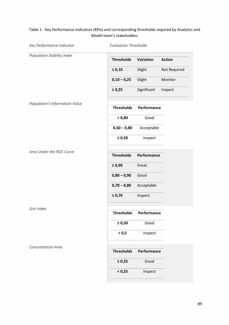
89
Table 1 - Key Performance Indicators (KPIs) and corresponding thresholds required by Analytics and
Model team’s stakeholders
Key Performance Indicator Evaluation Thresholds
Population Stability Index Thresholds Variation Action
≤ 0,10 Slight Not Required
0,10 – 0,25 Slight Monitor
≥ 0,25 Significant Inspect
Population’s Information Value Thresholds Performance
> 0,80 Good
0,50 – 0,80 Acceptable
≤ 0,50 Inspect
Area Under the ROC Curve Thresholds Performance
≥ 0,90 Great
0,80 – 0,90 Good
0,70 – 0,80 Acceptable
≤ 0,70 Inspect
Gini Index Thresholds Performance
≥ 0,50 Good
< 0,5 Inspect
Concentration Area Thresholds Performance
≥ 0,25 Good
< 0,25 Inspect

90
Sales Distribution (Percentage per propensity score percentile)
Sales Rate (Percentage per propensity score percentile)
Variables’ Characteristic Stability Index Thresholds Variation Action
≤ 0,10 Slight Not Required
0,10 – 0,25 Slight Monitor
≥ 0,25 Significant Inspect
Variables’ Information Value Thresholds Performance
> 0,80 Good
0,50 – 0,80 Acceptable
≤ 0,50 Inspect
While Analytics and Models team focused on model prediction accuracy performance, the Marketing
Campaign members required more business-oriented metrics, namely the number of clients listed and
the number of clients contacted for each campaign, contact and sales rate, and the total number of
sales per campaign. While not requiring thresholds for most metrics, Marketing Campaigns team
stakeholders established thresholds for marketing campaigns’ sales rate at the end of each commercial
cycle in accordance with Table 2.
Table 2 - Thresholds for marketing campaigns’ sales rate at the end of each commercial cycle
Thresholds Performance
≥ 1% Good
< 1% Inspect
All in all, considering that both teams expressed rather distinct demands, KPIs, and overall goals for
the project at hand, it was decided the development of two monitoring reports, each targeted towards
one specific team’s needs.

91
Requirement Elicitation
In this next phase, stakeholders’ expectations for the report layout, design, and interactivity, as well
as requirements for the visuals and thresholds’ encoding, were discussed.
Firstly, the usage of the bank’s official Power BI theme was requested for consistency purposes.
Therefore, design aspects such as the lettering font and colour palette have been laid out.
With regard to the Analytics and Models team’s report, functional requirements encompassed the
possibility of selecting the month or months under analysis and the inclusion of a filtering mechanism
to select the propensity model being analysed. Additionally, it was required for visuals used to allow
the display of several months’ performance and for the established metrics’ thresholds to be encoded
according to a specific colour scheme.
In turn, the Marketing Campaigns team required a more complex visualization report. On the one
hand, they expected to be able to visually compare two adjacent months (i.e., the selected month
against the previous month) for the number of contacts and sales, as well as for the contact and sales
rates of specific campaigns. In addition, they requested the possibility of filtering this information per
campaign codes or financial products marketed. Illustratively, if a user selected a certain product, then
only information pertaining to campaigns marketing the selected product should be displayed.
Furthermore, it was also requested the inclusion into the report of a visual encoding of a table
produced by the Marketing Campaigns team at the end of each month to summarize campaign results.
Moreover, this team presented additional functional requirements, requesting for the comparison of
the sales rate between commercial cycles. With regard to this comparison, it was also expected to be
possible to select the commercial cycles being analysed, as well as to filter sales rate information by
campaign code, marketed product, marketing channel, and an indicator of whether or not the
marketing leads incorporated a model’s propensity scores.
Lastly, Marketing Campaigns team requested the best and worst-performing campaigns to be
identified, as well as for a display of the evolution of the number of contacts and sales rate for as long
as a specific campaign has been active.
Data Collection and Design
During this phase, the necessary data to assemble the model monitoring reports was identified,
extracted, transformed, and loaded into Power BI Desktop’s application.
For the first report, targeted at Analytics and Models team, the performance metrics requested were
already calculated and stored in a SAS table. This table featured five columns, which are briefly
described in Table 3.

92
Table 3 - Column names and respective descriptions included in the SAS table provided by the
Analytics and Models team for reporting propensity model performance
Column Description
Model This column featured an abbreviation of the propensity model to which
the metric column corresponds to
Month This column featured a concatenation of the year and month of the
propensity scores the metric evaluates
Metric This column featured the name of the metric being evaluated
Sub_Metric This column featured each of the percentiles for which the Sales Rate and
Sales Distribution metrics were evaluated and assumed the value “Total”
for the remaining metrics
Value This column featured the value of the metric named in the field “Metric”,
evaluated on the propensity scores of the model identified in “Model”,
generated for the month “Month”, for each Sub_Metric (when applicable)
Conversely, the data required for constructing the Marketing Campaigns team’s report was collected
from five different SAS tables, stored across four different SAS libraries, as reported in Table 4.
Table 4 - SAS Tables, and their respective SAS Libraries, consulted for extraction and transformation
tasks underlying Marketing Campaigns team’s monitoring report
SAS Library SAS Table Description
Datamart Histcomunic Information pertaining to past marketing campaigns, namely
campaign code, code of the marketed product, marketing
channel used, date of contact, pseudo-unique customer identifier
and indicator of customer response
Vendas Vendas_Globais Information pertaining to product sales, including pseudo-unique
customer identifier, code of the product sold and date of sale
RR X_Cod_Produto Information matching the product codes to a product description
Luisaf Ac_Vend_4 Information pertaining to marketing campaigns results per
commercial cycle (only included campaigns marketed over
“human channels”)
Luisaf Ac_Vend_cnh_4 Information pertaining to marketing campaigns results per
commercial cycle (only included campaigns marketed over “non-
human channels”)

93
The bank characterizes its marketing channels into “human” and “non-human” based on whether they
require direct interaction between marketer and customer. As such, marketing campaigns presented
to the customer at the bank’s branch, or marketing communications performed over a phone call, by
either the account managers or the bank’s call centre, are considered to integrate the “human
channels”. Otherwise, marketing communications over email, SMS, or app notification, for example,
are included in the “non-human channels”.
Apart from SAS tables, additional data sources were consulted for data collection purposes. One of the
most relevant was an Excel file containing a pairing of the existing propensity models with codes of
campaigns whose marketing leads integrated propensity scores.
Required Extract, Transform, Load (ETL) steps were carried out on Base SAS Software, via SAS
Windowing Environment, given that most of the required information was stored in SAS Tables.
After prepping the datasets for the Construction and Validation phase, they were exported to a SQL
Server database to allow for Power BI Desktop to import them as data sources using the Get Data
functionality.
Finally, considering all the elicited requirements, a low-fidelity prototype of the reports’ layout and
visualizations was sketched on blank paper sheets. This product was iterated by integrating feedback
from the considered stakeholders before moving onto the next phase.
Construction and Validation
During this phase, the prototyped reports were reproduced using Power BI Desktop. The bank’s official
Power BI theme was applied, complying with the user requirement reported during the Requirement
Elicitation phase. Further design details have been discussed in collaboration with the stakeholders.
Snapshots of the outputs of this phase are presented in Figure 2 until Figure 6.
(a.1)
(a.2)
Figure 2 - Pages (a.1) and (a.2) composing the monitoring report targeted towards Analytics and
Models team’s analysts
As presented in Figure 2, the monitoring report developed to assist the Analytics and Models team’s
analysts relies on six matrix visuals and colour encoding to represent the required KPIs and their
respective thresholds. Additionally, it features two filtering mechanisms for selecting the model and

94
month(s) under analysis. For the model slicer, and per the request of the end-users, only one model
can be selected at a time. On the other hand, the month slicer allows for multiple item selection.
Filtering mechanisms, such as Power BI’s slicer, enable the users to dynamically adjust the displayed
information, and focus on information of interest.
The matrix visual is s structured table-like format that is easy to interpret and consult. The colours
selected by the end-users of this report for threshold encoding are reported in Table 5.
Table 5 - Colour specifications in hexadecimal values used for encoding the KPIs’ thresholds on the
Analytics and Models team’s report
Colour HEX Colour Code
#01B8AA
#B3C100
#F2C80F
#FD625E
Next, with regard to the Marketing Campaigns team, the first two pages of their monitoring report are
displayed in Figure 3.
(b.1)
(b.2)
Figure 3 - Pages (b.1) and (b.2) included in the monitoring report targeted towards Marketing
Campaigns team’s analysts
As presented in Figure 3, the page (b.1) of the monitoring report developed to assist the Marketing
Campaigns team’s analysts features bar chart visualizations to provide a fast visual comparison
between the selected and previous months. Additionally, filter mechanisms to select the financial
product marketed and the marketing campaign were also developed. On the top of this page were
included Power BI cards summarizing main KPIs.

95
On page (b.2) of the report, in accordance with the elicited requirements, it was included a
representation of the table summarizing campaign results, produced by the Marketing Campaigns
team at the end of each month.
(b.1.1)
(b.1.2)
(b.1.3)
(b.1.4)
Figure 4 - Different filtering settings for page (b.1) of the monitoring report targeted towards
Marketing Campaigns team’s analysts
In Figure 4 are displayed the filtering capabilities of page (b.1) of Marketing Campaigns team’s
monitoring report. When designing this page, it was required by the stakeholder not only to be possible
to filter the displayed information based on the financial product, marketing campaign, and month
under analysis but also that these filtering mechanisms be synchronized. As such, in (b.1.2), when
selecting a specific financial product, automatically, the list of marketing campaigns is updated to only
include campaigns marketing the selected product. The reverse scenario is represented in (b.1.3).

96
(b.3)
(b.4)
(b.5)
(b.6)
Figure 5 - Pages (b.3), (b.4), (b.5) and (b.6) included in the monitoring report targeted towards
Marketing Campaigns team’s analysts
As presented in Figure 5, pages (b.3) and (b.5) of the monitoring report developed to assist the
Marketing Campaigns team’s analysts pertain to the commercial cycle’s results for campaigns
marketed through human channels.
In more detail, page (b.3) displays sales rate information per product, campaign, channel, and
commercial cycle through a matrix visual. Per the requirement of this report’s end-users, the sales rate
information on this visual was extended by colour encoding it according to the specified thresholds.
The colours selected by the end-users of this report for threshold encoding are reported in Table 6.
Table 6 - Colour specifications in hexadecimal values used for encoding the sales rate thresholds
Colour HEX Colour Code
#B3C100
#FD625E
At the top right corner of page (b.3), Power BI cards summarize the main KPIs, according to the current
filtering selection. The amount and focus of the displayed information can be controlled by the user

97
through a set of five slicers for campaign code, commercial cycle, channel, product, and whether to
consider only campaigns whose leads integrated model propensity scores.
Additionally, four other Power BI cards were included in the header to help the user perceive which
filters are currently on effect.
Furthermore, page (b.4) features several different visuals providing a mixture of an overview of a
marketing campaign’s performance since they have first launched with performance indicators for the
selected commercial cycle.
More specifically, a Power BI’s funnel chart is employed to assist the visualization of the relative
proportion of clients listed for a marketing campaign, the number of clients which were contacted in
reality, from those the number of clients who expressed intention of purchasing the marketed product
and lastly, the number of clients who actually bought the product.
In turn, pie charts are applied to encode the distribution of listed clients, contacted clients and sales
per marketing channel in the selected commercial cycle, and scatterplots are used to overview contact
and sales rate since the campaigns have launched.
Two table visuals have been introduced into this page during the Validation phase, per request of the
stakeholders. These two visualizations represent information regarding the number of listed clients,
contacted clients, contact rate, number of clients denoting purchase intention, purchase intention
rate, number of sales and sales rate per product and per campaign.
Additionally, at the right top corner, the designation of the three best and worst-performing marketing
campaigns for the selected commercial cycle have been included, fulfilling another elicited
requirement.
Once again, the focus of the displayed information can be tuned through three filtering mechanisms
for campaign code, commercial cycle, and whether to consider only campaigns whose leads integrated
model propensity scores.
The same visualizations and filtering mechanisms have been reproduced in pages (b.5) and (b.6) for
campaigns marketed through non-human channels.

98
(b.3.1)
(b.4.1)
(b.5.1)
(b.6.1)
Figure 6 - Different filtering settings for pages (b.3), (b.4), (b.5) and (b.6) of the monitoring report
targeted towards Marketing Campaigns team’s analysts
Figure 6 displays some of the filtering capabilities of pages (b.3), (b.4), (b.5), and (b.6) of the Marketing
Campaigns team’s monitoring report.
On page (b.3.1), by using the slicers to filter for the commercial cycles of 201901, 201902 and 201903,
as well as to display only sales rate information pertaining to campaigns marketed through the bank’s
branch (sucursal, in Portuguese) channel, the content of the Power BI cards included in the header is
updated to reflect the filtering settings. This functionality was included to assist the user in perceiving,
which filtering settings are currently put in place. In addition, besides filtering the sales rate
information of the matrix visual, also the KPIs in the top right corner are updated to reflect the current
filtering scenario.
On page (b.4.1), only campaigns including propensity model’s scores into their leads were considered.
From these, a single campaign has been selected through a multiple selection-type slicer visual. As
such, both table visuals, as well as the funnel, pie, and scatter charts, alongside the Sales Rate Power
BI card, have been updated to comply with the filtering settings. In turn, the three best and worst-
performing campaigns remained unchanged as it was required them not to be affected by the slicer
visuals.
For page (b.5.1), only product and campaign information have been filtered. Firstly, on the product
slicer, the Credit Card product has been selected. As a result, the remaining slicers have been updated

99
only to include campaign codes, commercial cycles, and non-human channels available for campaigns
marketing the chosen product. Additionally, three marketing campaigns have been chosen from the
set of available campaigns. This selection was reflected in the card visuals included in the header. KPIs’
card visuals at the top right corner, as well as the sales rate matrix visual, have been updated
accordingly.
Lastly, on page (b.6.1), on the first table visual referring to marketing campaign KPIs per product, two
financial products have been selected by clicking on their respective rows while pressing the control
key. Subsequently, on the remaining campaign-specific visuals, the data pertaining to the selected
financial products have been highlighted. With this, the users can be provided with a relative
comparison of the contribution of campaigns marketing the chosen products for the different KPIs. As
in previous pages, the Power BI card included in the header has been updated to reflect the number
of campaigns marketing the chosen products. The Power BI sales rate card has also been updated
according to the filtering scenario described.
Maintenance
After receiving the approval of the involved stakeholders, the monitoring reports were published into
the Power BI App, in order to be made available and integrated into business analysts’ monitoring
frameworks.
Every month, the data sources will be updated to include new data. Periodical re-evaluations of the
end-users needs and requirements will be carried out in order to address identified problems or
improvement opportunities.
Conclusions
In the last decade, Business Intelligence (BI) has been gaining increased attention for leveraging data
to improve marketing, sales, and customer service processes. As such, the usage of BI tools and
technologies, such as reports and dashboards, has become increasingly widespread, allowing business
executives to make data-driven decisions by providing support for planning, presentation,
communication, monitoring, and analysis.
In this project, Power BI reports are developed for facilitating propensity models’ performance
monitoring tasks. With this goal in mind, two distinct reports have been constructed. The first report,
targeted at Analytics and Models team, featured model prediction accuracy KPIs. In turn, the report
designed to assist the Marketing Campaigns team’s business analysts was centred around more
business-oriented metrics.
The developed Power BI reports have been published and integrated into both teams’ monitoring
frameworks. For maintaining the reports and ensuring their compliance with changing user
requirements, periodical empirical evaluations will be performed. Subsequently, future improvements
will focus on addressing identified usability problems, impediments, or limitations as well as meeting
new user needs and requirements.

100
9.3. APPENDIX C – PROJECT: LEASING PRODUCTS PURCHASE PROPENSITY MODEL
With the rapid development of data mining technologies and data availability in financial fields, like
the banking sector, several organizations have recognized the importance of leveraging diverse,
comprehensive data for user modelling, in order to develop precise marketing strategies. Devising such
strategies requires an in-depth understanding of user behaviour, namely with regard to product
purchase likelihood.
In line with this sector trend, the Portuguese private commercial bank providing the data for this
project has been innovating its organizational and operational processes through the development
and deployment of decision support systems assisting sales processes and one-to-one marketing
efforts. In particular, several prediction and classification models directed at retail customers have
been implemented by a specialized team and integrated into the bank’s Retail Marketing Division’s
processes.
Contrastingly, decision support systems assisting enterprise marketing efforts are still very scarce. To
mitigate this shortage of integrated intelligent decision technologies in enterprise marketing
processes, the bank has envisioned several initiatives for the development of predictive models for
better understanding corporate clients’ behaviour. One such initiative pertains to the development of
a propensity model for predicting the likelihood of leasing products purchase by corporate clients.
Problem Definition
The goal of this project is to predict short-term leasing products purchase by the bank’s corporate
clients. Identifying potential customers who are likely to acquire leasing products in the following
month allows for customer prioritization for personalized marketing campaigns. By suggesting the
right product, to the right customer, at the right time, not only can the bank increase the efficiency
and effectiveness of its sales representatives, it can also improve its customers’ satisfaction, leading to
increased corporate profitability and customer loyalty.
In sum, this problem is formulated as a regression problem where the output of the predictive model
denotes the probability of each corporate client purchasing leasing products in the following month.
The rationale behind predicting monthly acquisitions pertains to Enterprise Marketing Division’s leads
generation processes’ execution frequency. Such processes are executed at the end of each
commercial cycle and updated every month, thus producing a monthly listing of suggested marketing
and sales client contacts.

101
Methodology
Leasing product purchase predictive model was developed on SAS Enterprise Miner 6.2, a proprietary
software, and the main predictive analytics tool employed by the bank. Furthermore, as the bank’s
data repository is stored in SAS tables, Base SAS Software, via SAS Windowing Environment, was used
for data collection tasks.
Given the usage of SAS Enterprise Miner software, Sample, Explore, Modify, Model, Assess (SEMMA)
methodology was adopted for this project. Developed by the SAS Institute, it can be defined as “a
logical organization of the functional toolset of the SAS Enterprise Miner”, thus making it a suitable
standard for implementing this predictive modelling application.
In order to model leasing product purchase behaviour, as specified by SEMMA methodology, and
following the data collection phase, an exploratory data analysis was conducted aiming to extract initial
insights from the available data. Next, a variable transformation and selection phase was performed
in order to reduce the dataset’s dimensionality and remove noisy, irrelevant, and redundant features.
Lastly, the proposed Meta-Level Hybrid 16 model is implemented, evaluated, and compared with three
state-of-the-art baseline models, namely Decision Tree, Gradient Boosting, and Logistic Regression.
Experimental Results and Discussion
In this section, a high-level description of the dataset supplied by the bank is provided. Next, the
Modification phase’s tasks are briefly overviewed. The evaluation methodology and performance
metrics calculated for model comparison are then defined. At last, experimental results are reported
and discussed.
The Dataset
To evaluate the different algorithms, extensive experiments were conducted on a real-world customer
dataset provided by a Portuguese private commercial bank, as part of a research internship program.
This raw dataset included 160.238 unique corporate clients, 1499 independent variables, and leasing
product monthly sales from January 2018 until September 2019.
Due to data security and privacy bank policies, customer name and other unique identifiers, such as
Taxpayer Identification Number, were pre-excluded from the provided real-life dataset. In turn, the
bank’s corporate clients were referred to via a pseudo-unique identifier.
According to the bank’s security, privacy, and marketing processes’ requirements, only active,
segmented, and consenting clients were included. These filters were applied in light of marketing
campaigns’ requirements that state that, in order for the bank to contact a client in the scope of a
marketing campaign, the client must be active and segmented, and they must also have consented to
be contacted. According to the bank’s guidelines, a client is considered active when they have made
16 A model learned by the Gradient Boosting algorithm replaces the original data and becomes the new input for
a Logistic Regression algorithm

102
at least one transaction, on their initiative, in the last 6 months. By this definition, transactions such as
incoming bank transfers and direct debit payments are not to be counted as own-initiative
transactions. Segmented clients refer to clients who are primary holders of a current account and,
lastly, consenting clients denote the bank’s clients who have consented to the use of their data for
marketing and analytics purposes and who also consented to be contacted within the ambit of
commercial campaigns. This last filter ensures the model’s compliance with the European Union’s
General Data Protection Regulation (GDPR).
As stated in the problem definition, the propensity model should predict, based on a set of predictors
collected at the end of each month, leasing product acquisition by corporate clients in the following
month. As such, the regression target was defined as a binary variable assuming the value 1 in cases
where the corporate client acquired leasing products up to one month from the reference date and
assuming the value 0 otherwise.
As the first step after data collection, the provided dataset was split into training and test sets, with a
proportion of 70:30, respectively.
Subsequently, an exploratory data analysis was conducted on the training set. Amongst the several
tasks undertaken during this phase were included the statistical analysis of independent variables,
their graphical representation for deriving initial insights, and the analysis of potential categories’
aggregation and numerical variables’ binning.
With the gathered knowledge about the data, subsequent steps towards reducing the dataset’s
dimensionality were taken.
As previously mentioned, the provided dataset originally featured 1499 independent variables,
covering socioeconomic and behavioural information about the bank’s corporate customers, as well
as financial indicators of the clients’ relationship with the bank. Additionally, it also featured
information regarding the clients’ current portfolio, past product purchases, and customers’ response
to previous marketing campaigns for the 19-month period of January 2018 until September 2019.
Given the high dimensionality of the dataset, and relying on the knowledge derived from the
exploratory analysis conducted, data cleaning tasks have been performed so as to prepare the data for
modelling.
First, 149 variables having a percentage of missing valued observations higher than 10% were
identified. Since, regardless of the imputation approach, missing values treatment is a perturbation of
the original data, these 149 features have been removed from the dataset.
After having handled features with missing values, 328 variables with mean, mode, and median equal
to zero have been removed from the dataset. Deleted features consisted mostly of interval variables
pertaining to either socioeconomic profile information or financial indicators of the client’s
relationship with the bank.
Lastly, 393 features with zero or almost zero variance (i.e., standard deviation strictly less than 0.001)
have been removed. Deleted features consisted of nominal and binary features flagging, for instance,
socioeconomic indicators such as whether that corporate client is listed, whether it is a start-up
company, or whether it is an import-export business.

103
Information regarding the number of variables removed from the dataset at each of the
aforementioned data cleaning steps is summarized in Figure 1.
Figure 1 - Data cleaning steps for dimensionality reduction and prepping the data for modelling
After data cleaning, the training and test sets comprised a total of 160.238 unique corporate clients,
628 input variables, 1 binary target variable, and 1 pseudo-unique client identifier.
The distribution of input variables’ data types is presented in Table 1.
Table 1 - Distribution of the independent variables across data types
Data Type Number of independent variables
Binary 386
Interval 218
Nominal 23
Ordinal 1
As reported in Table 1, more than 61% of the remaining independent variables are binary features,
followed by interval variables, totalling almost 35%, and nominal features accounting for the remaining
4% of the number of independent attributes.
Modification Phase
During the Modification phase, variable transformation, variable selection, and dataset resampling
steps were taken.
With the help of the Transform Variables node of SAS Enterprise Miner, several variable
transformations have been tested for interval and categorical features. Additionally, since Logistic
Regression models assume no multicollinearity between independent variables, a correlation analysis
of the input features was performed in order to remove redundant highly correlated features from the
dataset.

104
Lastly, given the severe unbalance of our dataset (i.e., every month only less than 1% of the bank’s
corporate clients acquire leasing products) an undersampling of the most frequent target class,
corresponding to the non-purchase event (i.e., target assuming the value 0), was performed.
Evaluation Methodology and Performance Metrics
As previously mentioned, prior to the data exploration phase, the dataset was split into test and
training sets, with the former accounting for 30% of all observations, and the latter for the remaining
70%. All four regression models were trained on the training set data and afterward evaluated on the
test set, so as to provide a more reliable performance estimate.
The metrics calculated and collected for model performance comparison were selected based on their
widespread employment for assessing propensity models’ performance. As such, experimental results’
discussion and analysis were based mainly on five metrics, namely Mean Square Error (MSE), Root
Mean Square Error (RMSE), Kolmogorov-Smirnov Statistic (KSS), Misclassification Rate (MR), and ROC
Index (ROC), measured on both the training and test sets.
Results and Discussion
In this section, the fitness of the proposed models is assessed through the aforementioned evaluation
metrics. Performance results for each of the considered regression algorithms are presented in Table
2.
Table 2 - Mean Square Error (MSE), Root Mean Square Error (RMSE), Kolmogorov-Smirnov Statistic
(KSS), Misclassification Rate (MR), and ROC Index (ROC), measured on both the training and test sets,
for Decision Tree, Gradient Boosting, Logistic Regression, and Meta-Level Hybrid regression models
Decision Tree Gradient Boosting Logistic Regression Meta-Level Hybrid
MSE Train Set 0.122640 0.103671 0.093020 0.085934
Test Set 0.120033 0.098799 0.088884 0.082332
RMSE Train Set 0.350200 0.322485 0.304991 0.293145
Test Set 0.346458 0.314323 0.298134 0.286935
KSS Train Set 0.763000 0.782000 0.780000 0.805000
Test Set 0.771000 0.820000 0.815000 0.820000
MR Train Set 0.142408 0.115183 0.109948 0.099476
Test Set 0.114355 0.099757 0.097324 0.094891
ROC Train Set 0.915000 0.929000 0.934000 0.934000
Test Set 0.920000 0.923000 0.925000 0.930000

105
Experimental results show that the Meta-Level Hybrid model is able to achieve the most accurate
prediction, slightly outperforming state-of-the-art baseline models for all considered metrics.
A more in-depth look into the proposed Meta-Level Hybrid model is presented in Figure 2, by analysing
its cumulative percentage of captured response.
Figure 2 - Cumulative Percentage of Capture Response for the Meta-Level Hybrid regression model
(in green) against the baseline curve (in grey)
In the chart displayed in Figure 2, the cumulative proportion of sales (i.e., the events where the target
equals to 1) that are captured in each percentile is plotted against the number of sales when no model
is being used 17.
From the analysis of this figure, it can be seen that, by using the Meta-Level Hybrid regression model,
50% of all considered corporate clients account for approximately 90% of all leasing product purchases.
As such, integrating this model into leads generation processes would allow account managers to
achieve sales objectives while contacting a smaller number of clients. Therefore, the sales contacts
efficiency and, subsequently, their conversion rates could improve significantly.
One the other hand, leasing product sales contacts would be better targeted at customers who truly
need or have an interest in purchasing such products, while customers who are not interested in
buying them would not be excessively disturbed, thus increasing customer satisfaction.
17 Jaffery, T., & Liu, S. X. (2009). Measuring campaign performance by using cumulative gain and lift chart.
SAS Global Forum, 196.

106
Apart from assessing model performance, an analysis of the most relevant features for modelling the
problem at hand was also carried out.
Figure 3 displays the importance attributed to the top 7 independent variables by the Gradient
Boosting component of the Meta-Level Hybrid regression model.
Figure 3 - Feature Importance attributed by the Gradient Boosting component of the Meta-Level
Hybrid regression model to the top 7 independent variables
From the interpretation of Figure 3, it can be reasoned that the model relies mainly on five
independent attributes for leasing product sales likelihood prediction. Next, each of the top 7 features
included in Figure 3 will be analysed with regard to the model’s target. In relation to their data type,
from these seven features, four are binary, while three are interval variables.
From Figure 4 to Figure 10, the event of target equal to 1 is referred to as “Clients who acquired leasing
products” while the complementary event is designated “Clients who did not acquire leasing
products”.
Firstly, in Figure 4, binary Variable #1’s distribution per target class is reported.

107
Figure 4 - Distribution of Variable #1 per leasing products purchase propensity model’s target class
Variable #1 relates to a specific leasing product’s contracted amount one year previous to the
reference date. As such, through the analysis of Figure 4, it can be seen that clients who possessed this
specific leasing product one year before are less likely to purchase it again at the time of the reference
date.
Variable #2 pertains to the number of a specific type of transfer performed by corporate clients via
internet channels. On this basis, Figure 5 displays the binned distribution of Variable #2, for all
corporate clients, as well as for clients who did and did not acquire leasing products.
Figure 5 - Distribution of Variable #2 (after binning), for all corporate clients (in grey), as well as for
clients who did (in dark green) and did not (in light green) acquire leasing products
From the interpretation of Figure 5, customers performing less than 10 such transfers have a higher
probability of not acquiring leasing products. On the other hand, corporate clients performing 30 to 40
transfers are more likely to purchase the target products.
Next, in Figure 6, binary Variable #3’s distribution per target class is reported.

108
Figure 6 - Distribution of Variable #2 per leasing products purchase propensity model’s target class
Variable #2 relates to another specific leasing product’s contracted amount one year previous to the
reference date. By interpreting Figure 6, it can be seen that clients who possessed this specific leasing
product one year before are slightly less likely to purchase it again at the time of the reference date.
Variable #4 pertains to the number of marketing and communication campaigns directed at each
corporate client. In Figure 7, the distribution of Variable #4, after having been binned, for all corporate
clients, as well as for clients who did and did not acquire leasing products, is presented.
Figure 7 - Distribution of Variable #4 (after binning), for all corporate clients (in grey), as well as for
clients who did (in dark green) and did not (in light green) acquire leasing products
While not having discriminative boundaries as clear as Variable #2, from the interpretation of Figure
7, it can be reasoned that customers receiving less than 10 marketing contacts have a slightly higher
probability of acquiring leasing products. On the other hand, corporate clients who were contacted for
more than 10 communication or marketing campaigns are more likely not to purchase the target
products.
In Figure 8, the distribution of the binary Variable #5 per target class is presented.

109
Figure 8 - Distribution of Variable #5 per leasing products purchase propensity model’s target class
Variable #5 relates to the number of products each client acquired from one year previous to the
reference date. As reported in Figure 8, clients who did not acquire any products during the last 12
months are less likely to acquire leasing products at the time of the reference date. Conversely,
corporate clients having purchased some financial products have a slightly higher probability of also
purchasing the target products.
Variable #6 pertains to the number of days the account balance remained negative after overdrawing.
Figure 9 presents the distribution of Variable #6, after having been binned, for all corporate clients, as
well as for clients who did and did not acquire leasing products.
Figure 9 - Distribution of Variable #6 (after binning), for all corporate clients (in grey), as well as for
clients who did (in dark green) and did not (in light green) acquire leasing products
By interpreting Figure 9, it can be seen that customers who restore their account balance in less than
10 days are more likely to (be allowed to) purchase leasing products. On the other hand, corporate
clients who, after overdrawing, leave their accounts with a negative balance for more than 1 month
are much less likely to (be allowed to) purchase the target products.
Lastly, the distribution of the binary Variable #7 per target class is presented in Figure 10.

110
Figure 10 - Distribution of Variable #7 per leasing products purchase propensity model’s target class
At last, Variable #7 relates to the total amount of credit liabilities owned by corporate clients. In Figure
10, it is reported that clients who have very small amounts of credit liabilities with the bank are much
more likely to acquire leasing products.
Ex-Post Backtesting
In order to emphasize the added benefit of the proposed propensity model to marketing and sales
processes, backtesting for the month of October 2019 was conducted. Backtesting the proposed model
allows for an evaluation of how it would have performed ex-post. The main purpose of this analysis
was to provide an assessment of the commercial viability of the proposed model. More specifically, to
stress the model’s aptitude to identify potential promising corporate clients for purchasing the target
leasing products.
The results for the backtesting of the Meta-Level Hybrid model’s performance are summarized in
Figure 11.
Figure 11 - Ex-Post Backtesting of Meta-Level Hybrid model’s performance for the month of October
2019
Per analysis of Figure 11, it can be seen that almost 50% of all registered leasing sales during the
surveyed month occurred from corporate clients listed among the 10% more likely to acquire such
products according to the proposed model. Additionally, among those same 10% corporate clients, the

111
probability of a client acquiring the target products is far greater than the probability that they do not
acquire them. On this basis, backtesting results support the model’s potential for improving sales
contacts’ conversion rates and better focusing sales representatives’ commercial efforts.
Conclusions
The rapid development of data mining technologies and data availability in the banking sector has
given rise to the need to equip sales representatives, bankers, and account managers with tools that
support precise marketing strategies leveraging in-depth customer knowledge.
In this project, a Meta-Level Hybrid regression model is proposed for the problem of predicting short-
term leasing products purchase by a bank’s corporate clients.
This thesis considers an anonymized dataset provided by a Portuguese private commercial bank, as
part of a research internship program. Prior to modelling and assessment phases, an exploration of
the provided data was conducted with the goal of generating initial insights into the prediction
problem, and the relationship between predictors and the target variable.
On this basis, the proposed model has been implemented, evaluated, and compared against three
state-of-the-art baseline models, them being Decision Tree, Gradient Boosting, and Logistic
Regression. Model performance was assessed over five evaluation metrics, namely Mean Square Error,
Root Mean Square Error, Kolmogorov-Smirnov Statistic, Misclassification Rate, and ROC Index,
measured on both the training and test sets.
According to the obtained experimental results, the proposed Meta-Level Hybrid regression model
outperforms the remaining baseline algorithms for all evaluation metrics considered. Additionally, ex-
post backtesting was conducted in order to more reliably assess the commercial viability of the
proposed model. This experiment stressed the model’s aptitude to identify potential promising
corporate clients for purchasing the target leasing products and, thus, confirming the model’s added
value to marketing and sales processes.
Ultimately, likelihood propensity estimates will be integrated into marketing and sales leads
generation processes and be passed onto the respective account managers. Therefore, the proposed
algorithm will allow to more accurately target marketing campaigns, anticipating clients’ needs, and
reducing client contacts, leading to increased customer satisfaction and profitability.
The planning and integration of the proposed model into the bank’s marketing leads generation
process is underway. This experiment will feature a set of corporate clients, termed control group, for
whom the generated leads will not incorporate leasing products purchase likelihood predictions.
Future work directions will, thus, include the implementation and monitoring of the aforementioned
experiment. Given that a sufficiently long testing period is surveyed, it will be possible to confirm the
proposed model’s contributions and assess its real-world applicability, beyond ex-post and offline
evaluation metrics.

112
9.4. APPENDIX D – SYSTEMATIC LITERATURE REVIEW
To better understand the scientific background framing this work, as well as to adequately position its
contributions, a review of the state-of-the-art of Recommender Systems research was undertaken.
It was acknowledged that a comprehensive overview of Recommender Systems literature would be
too extensive18 on account of the vastness of available literature 19. Therefore, considering the data
used in this project is sourced from a banking institution, and similarly to previous works (Bogaert et
al., 2019), this thesis will focus on surveying the landscape of Recommendation Systems in the financial
services sector.
In the following sections, the state-of-the-art of Recommender Systems, applied to the financial sector,
will be summarized and analysed in terms of the year of publication, application domain,
recommendation techniques, underlying algorithms, and evaluation strategies and metrics.
Methodology
The following review work follows the guidelines for Systematic Literature Review (SLR) delineated in.
Contrarily from traditional (ad-hoc) literature reviews, this methodology constitutes a means to
analyse and interpret the available research in a meticulous, unbiased, and auditable way (Zhang et
al., 2011).
According to Systematic Literature Review guidelines, a Review Protocol should be developed prior to
the conduction of the review work in order to ensure the properties of reproducibility and impartiality
of SLR. For this reason, an SLR Protocol must clearly stipulate the procedure for identifying primary
studies addressing the defined review questions 20.
The different steps of the Review Protocol employed in this thesis are summarized in Figure 1.
18 Preliminary searches of Recommendation Systems, not yet restricted to financial services sector
applications, retrieved over 50.000 documents across the six digital libraries considered. 19 Beel, J., Gipp, B., Langer, S., & Breitinger, C. (2016). Research-paper recommender systems: a literature
survey. International Journal on Digital Libraries, 17, 305-338. 20 Kitchenham, B., & Charters, S. (2007). Technical report title: Guidelines for performing Systematic
Literature Reviews in Software Engineering, EBSE 2007-001. Keele University and Durham University Joint Report.

113
Figure 1 - Systematic Literature Review Protocol
Adapted from (Çano & Morisio, 2017).
The SLR Protocol employed in this thesis features twelve steps, which will be detailed in the following
subsections.
Review Questions, Search Query, and Digital Sources
The main purpose of this Systematic Literature Review is to understand how Recommender Systems
applied to the financial services sector have evolved, how they are implemented and evaluated, and
in which financial sector domains they are most commonly employed. To do so, the following review
questions, delineating the research scope, have been specified:
RQ1 – How is the volume of relevant Recommender Systems research, applied to the financial services
sector, distributed over the last decade?
RQ2 – In what financial services sector domains are Recommenders employed?
RQ3 – Which data mining and machine learning techniques are exploited for Recommendation
Systems implementation?
RQ4 – Which recommendation techniques are used for Recommenders applied to the financial
services sector?

114
RQ5 – Which evaluation methodologies are employed to assess Recommender performance?
RQ6 – What metrics are monitored when evaluating Recommender Systems?
Six digital libraries, listed in Table 1, were selected as the primary sources for Recommender Systems
publications. This selection took into account digital libraries considered in previous systematic review
works as well as their accessibility to external researchers (Zhang et al., 2011).
Other frequently used sources, namely IEEE Xplore (Zhang et al., 2011), were not considered as they
are indexed in at least one of the primary sources considered.
Table 1 - Digital libraries considered as primary sources for relevant documents retrieval
Digital Library URL
ACM Digital Library https://dl.acm.org/
B-On https://www.b-on.pt/
SAGE Journals https://journals.sagepub.com/
ScienceDirect https://www.sciencedirect.com/
Scopus https://www.scopus.com/
SpringerLink https://link.springer.com/
In this stage, preliminary searches 20 were conducted with the goals of assessing the volume of relevant
available literature and identifying frequently used terms pertinent to Recommender Systems research
in the financial services sector.
In order to derive the search terms, statistical analysis of the most frequently occurring term
combinations in the keywords, title, and abstract of financial Recommender System publications was
undertaken. In order to carry out this analysis, Python’s nltk and WordCloud textual analysis packages
were utilized.
The set of elicited terms capturing the concepts of interest was extended with usual synonyms,
culminating in the set of keywords listed in Table 2.
Table 2 - Set of relevant keywords and their synonyms
Keywords and Synonyms
Finance, Financial, Banking, Bank
Recommendation, Recommender
System, Engine, Algorithm, Model, Method, Approach

115
The derived search query was defined as follows ("Finance" OR "Financial" OR "Banking" OR "Bank")
AND ("Recommendation" OR "Recommender") AND ("System" OR "Engine" OR "Algorithm" OR
"Model" OR "Method" OR "Approach").
The exact search query’s codification was adapted in accordance with the specific syntax and filtering
criteria settings of the different digital libraries’ search engines. As a reference, Scopus’ search queries
are presented in Table 3.
Table 3 - Scopus’ queries for Initial Search and Retrieval, and Coarse Selection stages
Selection Stage Scopus’ Search Query
Initial Search and
Retrieval
TITLE-ABS-KEY(("Finance" OR "Financial" OR "Banking" OR "Bank") AND
("Recommendation" OR "Recommender") AND ("System" OR "Engine"
OR "Algorithm" OR "Model" OR "Method" OR "Approach"))
Coarse Selection TITLE-ABS-KEY (("Finance" OR "Financial" OR "Banking" OR "Bank") AND
("Recommendation" OR "Recommender") AND ("System" OR "Engine"
OR "Algorithm" OR "Model" OR "Method" OR "Approach")) AND (
DOCTYPE ( "ar" ) OR DOCTYPE ( "cp" ) ) AND ( ( PUBYEAR > 2008 ) AND (
PUBYEAR < 2020 ) ) AND ( SRCTYPE ( "j" ) OR SRCTYPE ( "p" ) ) AND (
LANGUAGE ( "English" ) )
Table 3 presents the search queries used for retrieving Recommendation System studies during the
Initial Search and Retrieval, and Coarse Selection stages of the SLR Protocol.
Selection of Papers
Initial Search and Retrieval
For initial search and retrieval, the search query was applied to the digital libraries’ search engines in
order to obtain all documents whose title, abstract, or keywords matched the elicited set of relevant
keywords and respective synonyms. In total, 13.810 studies were identified and retrieved by applying
the defined search query to the six digital libraries selected.
This study retrieval process was conducted on October 19th, 2019, and its results are summarized in
Table 4.
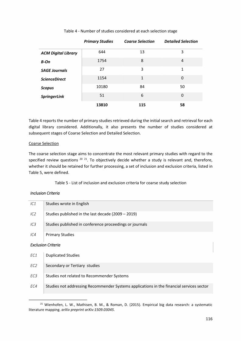
116
Table 4 - Number of studies considered at each selection stage
Primary Studies Coarse Selection Detailed Selection
ACM Digital Library 644 13 3
B-On 1754 8 4
SAGE Journals 27 3 1
ScienceDirect 1154 1 0
Scopus 10180 84 50
SpringerLink 51 6 0
13810 115 58
Table 4 reports the number of primary studies retrieved during the initial search and retrieval for each
digital library considered. Additionally, it also presents the number of studies considered at
subsequent stages of Coarse Selection and Detailed Selection.
Coarse Selection
The coarse selection stage aims to concentrate the most relevant primary studies with regard to the
specified review questions 20 21. To objectively decide whether a study is relevant and, therefore,
whether it should be retained for further processing, a set of inclusion and exclusion criteria, listed in
Table 5, were defined.
Table 5 - List of inclusion and exclusion criteria for coarse study selection
Inclusion Criteria
IC1 Studies wrote in English
IC2 Studies published in the last decade (2009 – 2019)
IC3 Studies published in conference proceedings or journals
IC4 Primary Studies
Exclusion Criteria
EC1 Duplicated Studies
EC2 Secondary or Tertiary studies
EC3 Studies not related to Recommender Systems
EC4 Studies not addressing Recommender Systems applications in the financial services sector
21 Wienhofen, L. W., Mathisen, B. M., & Roman, D. (2015). Empirical big data research: a systematic
literature mapping. arXiv preprint arXiv:1509.03045.

117
According to Table 5, if a study complies with all four inclusion criteria and does not verify any of the
defined exclusion criteria, then it can advance to the next study selection stage.
Park et al. (2011) have reported a rapid increase in Recommendation Systems publications between
2007 and 2010. Moreover, the last decade witnessed significant changes for the banking industry,
mostly related to the steady growth and widespread application of information technologies (Zibriczky,
2016). As such, a time span of 10 years was considered a suitable publication period for this review. As
such, only studies published from 2009 until 2019 were considered.
For this review, only primary studies were included. That is empirical research conducted by the
authors in order to answer specific research questions 20. Secondary studies (e.g., reviews of primary
studies) and tertiary studies (e.g., reviews of secondary studies) were excluded.
Due to the overlap among digital libraries, duplicated studies need to be identified and removed. The
duplicates removal was performed in accordance with Table 6.
Table 6 - Rules for duplicated studies removal
Digital Library Remove studies that are already present in…
Scopus ---
B-On Scopus
ACM Digital Library Scopus or B-On
ScienceDirect Scopus or B-On or ACM Digital Library
SAGE Journals Scopus or B-On or ACM Digital Library or ScienceDirect
SpringerLink Scopus or B-On or ACM Digital Library or ScienceDirect or SAGE Journals
The number of studies considered for detailed selection per digital library was very much impacted by
the rules presented in Table 6. For example, a SpringerLink sourced study will only advance towards
the next selection stage if it is not yet present in any of the other digital libraries considered. Given
that libraries such as Scopus and B-On partially index the other considered collections, it is expected
that they concentrate the majority of considered studies.
Since strictly processing all studies was not practical, in most cases, the abstract was examined in order
to decide whether the study should be retained. However, certain cases required other parts, namely,
introduction and conclusion, to be analysed.
After applying the inclusion and exclusion criteria, a list of 115 studies was obtained.

118
Detailed Selection
In this stage, a detailed selection of the studies was carried out by revising the content of every paper.
In order to arrive at the final list of primary studies, each paper was analysed based on the
completeness of the proposed algorithm’s description, its implementation, and its application to the
financial services sector.
Furthermore, some studies were still duplicated, typically due to being published in consecutive years
or different publications.
At last, the final set of 58 primary studies was identified. Their publication details can be consulted in
Annex A.
Data Extraction and Quality Assessment
Data extraction was undertaken on the final set of 58 primary studies. During this process, all relevant
data to approach the review questions must be gathered 20. The collected data items, as well as the
review questions they address, are synthesised in Table 7.
Table 7 - Data items collected during the Data Extraction process
Data Item Review Question
Publication Year RQ1
Application Domain RQ2
Recommendation Technique RQ3
Data Mining and Machine Learning Techniques RQ4
Evaluation Methodology RQ5
Evaluated Metrics RQ6
Challenges inherent to the Financial Sector RQ7
In order to confirm the consistency of the data extraction procedure, cross-checking was done on 20
arbitrarily selected papers (around 34%).

119
Synthesis and Analysis
In this subsection, the data extracted is synthesised and analysed in light of the specified review
questions.
RQ1 – How is the volume of relevant Recommender Systems research, applied to the financial services
sector, distributed over the last decade?
The final set of primary studies contained 58 studies published in conference proceedings and journals
over the last ten years (from 2009 until 2019). The distribution, according to the publication year, is
presented in Figure 2.
Figure 2 - Distribution of primary studies per publication year
According to Figure 2, the number of Recommender Systems’ publications applied to the financial
services sector denoted a significant increase between 2014 and 2015, with more than 77% of the
primary studies being published in the second half of the time span considered (from 2015 onwards).
The growth of the number of publications in recent years is an indicator of the intensifying demand for
Recommender Systems improving sales efficiency and automatizing decision-making in the financial
services sector, mainly due to recent changes in the banking industry, in particular developments in
mobile and digital banking (Urkup et al., 2018).
RQ2 – In what financial services sector domains are Recommenders employed?
In this thesis, for the purpose of overviewing the application areas of Recommender Systems, a
financial domain was considered a specific area of finance that can be duly delimited and typified
according to the properties of the items being recommended (Zibriczky, 2016).
On that account, the following financial domains were defined:
Financial Statements Auditing
In Financial Statement Auditing, an independent auditor examines the financial statements of a
company to corroborate the authenticity and completeness of the disclosed financial statements. In

120
this domain, the recommendation task is focused on pairing relevant text passages with legal
requirements 22.
Traditional Lending
In Traditional Lending, money is lent by a traditional financial lender, typically a bank, to an entity
(either a private individual or an organization), under contracted conditions. In this domain, the
recommendation problem is focused on matching borrowers with loan products offered by one or
multiple banks, satisfying the borrowers’ financial needs while also regarding their risk of default.
Venture Finance
Venture Capital constitutes initial funding provided by Venture Capital firms or funds for emerging
companies in exchange for private equity. The goal of Recommender Systems in Venture Finance is to
find adequate fits between emerging companies seeking funding and potential Venture Capital
investors.
Financial News
Financial News includes all news articles reporting conducted research or interviews regarding
economic matters, such as stock market trends, mergers, and acquisitions. In this domain,
Recommenders are tasked with suggesting previously unseen news articles on the basis of their
potential interest to the users.
Investment Management
A portfolio is a collection of differently weighted financial assets. In this domain, Recommenders’ task
is to manage portfolio composition by recommending asset allocation strategies in accordance with
the investor’s current portfolio and risk appetite.
Retail Banking
Retail Banking can be defined as the banking activities providing products and services to consumers
and small businesses through bank branches, call centres, ATMs, web and mobile platforms, or other
channels. Services and products offered by retail banks include transaction deposits, saving accounts,
credit cards, mortgages, personal loans, and insurance brokerage 22. In this domain, Recommender
Systems are mostly employed in order to recommend retail products and services, aiming to increase
sales representatives’ effectiveness.
P2P Lending
Peer-To-Peer (P2P) Lending is a type of microfinance solution through which individuals, organized
singularly or in teams, can invest in low-income individuals, groups or projects, via a P2P lending
marketplace. In this context, the goal of Recommender Systems is to appropriately pair lenders with
individuals or projects requiring loans (Zibriczky, 2016).
22 Sifa, R., Ladi, A., Pielka, M., Ramamurthy, R., Hillebrand, L., Kirsch, B., ... & Nütten, U. (2019, September).
Towards Automated Auditing with Machine Learning. Proceedings of the ACM Symposium on Document Engineering 2019, 1-4.

121
Stock Market
Stocks, representing ownership in a company, are traded in the stock market, where the pricing is ruled
by traders’ bids and offers. In this domain, a Recommender’s task is to suggest a stock purchase or sale
heeding the trader’s portfolio and the stocks’ buy and sell prices.
On the basis of the aforementioned financial domains, Figure 3 reports the distribution of
Recommender research across the financial sector’s application domains.
Figure 3 - Distribution of primary studies per application domains
According to Figure 3, the prevalent domain is Stock Market related recommendation, gathering
slightly more than 30% of the primary studies considered. However, P2P loans, retail products and
services, and portfolio recommendation also present considerable volumes of research, covering
around 48% of the reviewed papers. Financial News recommendation mustered almost 10% of the
review literature and reported contributions in Venture Finance, Traditional Loans, and Financial
Statements Auditing domains account for the remaining 10%.
RQ3 – Which data mining and machine learning techniques are exploited for Recommendation
Systems implementation?
This review question addresses the distribution of research according to the Data Mining and Machine
Learning techniques employed by the Recommendation Systems proposed in the set of considered
primary studies.
Data Mining techniques are purposed for the extraction of meaningful patterns from large quantities
of data (Park et al., 2011). On the other hand, Machine Learning techniques focus on learning a
classification or regression model from the training data 23.
Due to the significant overlap between the techniques employed in Data Mining and Machine Learning
fields 23, in this review, the implemented algorithms will simply be referred to as DM/ML techniques.
23 Buczak, A. L., & Guven, E. (2015). A survey of data mining and machine learning methods for cyber
security intrusion detection. IEEE Communications surveys & tutorials, 18(2), 1153-1176.

122
On this note, Figure 4 reports the distribution of Recommenders’ research according to the DM/ML
techniques implemented.
Figure 4 - Distribution of primary studies per implemented DM/ML techniques
As shown in Figure 4, a wide variety of DM/ML techniques is used for Recommender’s implementation,
with authors typically using diverse approaches when building the different components of the
proposed Recommendation System architecture.
For instance, in [P2], a Recommender for automating financial statements audit is proposed. The
recommendation task is dependent on matching the document under audit against a checklist of legal
requirements. To do so, the financial report and legal requirements’ text is pre-processed (included
steps are stemming and lemmatization) and then represented using n-grams, TF-IDF, and Matrix
Factorization vector space representations. Finally, the recommendation is based on the calculus of
similarity between the representation of each legal requirement and specific report structures (e.g.,
paragraphs, tables). Similarity measures employed are either Jaccard- or Tversky-index for n-gram
representation, or the cosine similarity in the case of vector space representations. Alternatively,
authors consider a supervised learning approach, by training a Logistic Regression receiving the
structure’s representation as input in order to predict the probability of relevance for a requirement.
Under the assumption that a specific structure could pertain to several requirements, authors also
propose a Feed-Forward Neural Network mapping a given structure to a binary relevance vector for
all the requirements. At last, in order to account for structural dependencies among legal requirements
and document structures, a Recurrent Neural Network using Gated Recurrent Units is also proposed.
From the interpretation of Figure 4, the most frequent technique is found to be reliant on the
calculation of distance or similarity measures for producing item recommendations.
Illustratively, in [P3] a model is proposed for estimating investors’ personalized stock preferences.
Under the assumption that automatic predictions regarding the interests of a user can be generated
by collecting the preferences from other users having similar investment philosophies, authors
combine users’ historical preferences and historical stock movements in a matrix they designate
movement-aware preference matrix. On this basis, the proposed model estimates the similarity

123
between two users using the cosine similarity between their row vectors in the movement-aware
preference matrix. As future work, authors propose deep learning strategies for better inferring
investors’ preferences.
In the majority of the studies reviewed [P1] [P9] [P37] [P41] [P51] [P52], the authors provided a
comparison between several algorithms’ performance in order to find the best-fitted model.
For instance, in [P1], the authors propose a Recommendation system for advising P2P borrowers on
the adequate type of loan according to interest rates and the likelihood of getting funded. To reach
this goal, they compare three feature selection algorithms (forward selection, backward selection, and
recursive selection) and employ four regression models, namely linear regression, an ensemble
regressor (i.e., Random Forest), Support Vector Machines (SVM) and k-Nearest Neighbours (k-NN)
algorithms. Finally, having predicted, for each client and each type of loan, a tuple of the interest rate
payable and the likelihood of success, they compute the Euclidean Distance between each predicted
tuple and the optimal case of 0% interest rate payable and 100% likelihood of successfully getting
funded, in order to generate the recommendation. At last, the authors propose deriving a sentiment
score from the borrower’s loan purpose description using VADER (Valence Aware Dictionary and
sEntiment Reasoner), a rule-based sentiment analysis tool, and assessing its impact on the likelihood
of getting funded.
However, about 27% of the reviewed studies implement only one machine learning algorithm in their
Recommendation System solution. Particularly, Association Rule Mining [P21], Neural Networks [P10],
Ensemble regressors and classifiers [P12], Correlation Coefficients [P14], and Matrix Factorization
[P35] [P50] techniques.
Around 10% of the reviewed studies explicitly reported having used feature selection/extraction (FSE)
methods to lessen the number of variables under consideration aiming to efficiently summarize the
input data [P9] [P49], reduce the computational requirements [P18] [P49], and enhance the predictive
model’s performance [P1] [P9] [P18]. Some of the employed FSE methods include Recursive Feature
Elimination (RFE), Forward and Backward Selection, f_regression, Principal Components Analysis
(PCA), and Non-Negative Matrix Factorization (NMF).
Finally, five problem classes were identified for recommending the most suitable item(s) for each user:
binary classification, multi-class classification, multi-label classification, single-output regression, and
multi-output regression.
Focusing on one specific product, binary classification tries to ascertain whether each user will
consume or purchase a certain item. Application examples found for this class of problems are
predicting whether a lender will fund a loan [P8], whether a bank customer will apply
for/subscribe/acquire a specific product [P9] [P18] [P42], and whether a news article is relevant [P15].
Still considering Recommenders suggesting only one product for each user, multi-class classification
problems select, out of the whole range of products, the one that is most likely to be bought by a
specific customer. These types of problems are often referred to as Next-Product-To-Buy (NPTB)
models. Amidst the reviewed studies, [P36] [P54] are structured as multi-class classification problems.
In the former study, the target is considered as the last financial product purchased by each customer.
While in the latter, each user is recommended the portfolio of the representative expert in the
community to which the user belongs. Multi-label classification, on the other hand, selects a set of the

124
k products most likely to be of interest to the user, considering the whole range of available products.
Amid the primary studies considered, multi-label classifiers are used to recommend a set of financial
products for cross-sell purposes [P5], to automatically find potential lenders, in a P2P lending
environment, for the target loan [P12], and to identify the most appropriate service selection, in order
to adjust the menu ordering in banking applications [P52].
Regarding regression problems, single-output regression was employed mostly to predict stock
prices/expected stock returns [P13] [P19] [P32]. However, it was also utilized in other application
domains, such as P2P lending [P49], where it was used to predict the likelihood of funding for a given
(lender; loan) pair. In this case, the best lender for a particular loan i can be found by solving argmaxi
(U, i) for all users in the U set. Analogously, the most suitable loan for a lender u to invest in can be
found by calculating the argmaxu (u, I) for all loans in the I set. Lastly, multi-output regression
problems are primarily used for predicting a vector of item consumption/acquisition probabilities for
each user. For instance, in the field of Financial Statements Auditing [P2], a Feed-Forward Neural
Network is proposed for mapping each passage from the financial statement under audit (i.e.,
considered the “user” of the Recommendation System) to a relevance vector for all the legal
requirements (i.e., the recommended items).
RQ4 – Which recommendation techniques are used for Recommenders applied to the financial
services sector?
Recommendation techniques found on the set of primary studies reviewed are Content-Based Filtering
(CBF), Collaborative Filtering (CF), Hybrid, and Knowledge-Based paradigms.
Among them, Content-Based and Collaborative Filtering are the most frequently employed techniques
for recommendation computation.
The distribution of primary studies across recommendation techniques is shown in Figure 5.
Figure 5 - Distribution of primary studies per recommendation paradigms
For this distribution, Demographic Filtering (DF), as well as CF-DF hybrids, were incorporated as
extensions of the Collaborative paradigm, as they differ in the nature of the input features but have
similar recommendation approaches.

125
Another perspective that was analysed was the distribution of DM/ML techniques according to the
underlying recommendation technique. A summary of the results is presented in Figure 6.
Figure 6 - Distribution of DM/ML techniques across recommendation paradigms
This analysis emphasised that the use of certain DM/ML techniques is highly dependent on the
recommendation paradigm employed. Namely, among the 58 primary studies examined, Correlation
Coefficients were found to be exclusively used with Collaborative Filtering approaches, while Time
Series Analysis was employed only in Content-Based Recommenders, applied to the Stock Market
domain.

126
As a result, the most frequently employed DM/ML techniques also vary in accordance with the
underlying recommendation paradigm. As shown in Figure 6, it is possible to denote that Collaborative
Filtering approaches mostly rely on Rule Mining, Correlation computation, K-Nearest Neighbours
algorithm, and Matrix Factorization methods. While Content-Based approaches, mainly due to the
need for item properties extraction, focus on Word Embedding and Text Vectorization techniques,
Knowledge Representation mechanisms (such as Ontologies), and Time Series Analysis (found in four
primary studies relating the forecast of stock prices/returns).
RQ5 - Which evaluation methodologies are employed to assess Recommender performance?
Review questions 5 and 6 examine the Recommenders’ evaluation process, namely the evaluation
methodologies (see Figure 7) and involved metrics (see Figure 8).
Figure 7 - Distribution of primary studies per evaluation methodologies
According to Figure 7, most studies report having evaluated the proposed algorithm(s) in comparison
against one or more baselines, usually chosen from the most widely implemented algorithms (e.g.,
kNN, MF) for the recommendation paradigm being employed.
Other studies also report kNN (Bobadilla et al., 2013) and Matrix Factorization techniques (Jannach et
al., 2012) as reference algorithms, in particular for Collaborative Filtering recommendation.
The second most used evaluation methodology relies on comparing either different parameter
configurations [P32] or variations of the proposed Recommender. That is, for instance, Recommenders
relying on different Feature Selection/Extraction techniques [P9], different classifiers or regressors [P2]
[P5], different ranking strategies [P20] [P44], and so on.
Among the considered primary studies, 16 report having split their dataset into train and test sets
when assessing the Recommender’s performance. Cross-validation was performed in 8 studies, and
backtesting was employed in two Recommenders for the Stock Market domain.
User studies and surveys were used in 4 cases, while comparison against domain experts was
undertaken in 3 studies. Both these evaluation methodologies require the involvement of users who
perform mainly subjective quality assessments and provide feedback about their perception of the
Recommendation System.

127
Finally, from the 8 primary studies which did not report evaluation, two indicated the evaluation of
their recommendation framework as future work [P41] [P53].
RQ6 – What metrics are monitored when evaluating Recommender Systems?
Regarding the metrics involved in the evaluation methodology, Figure 8 summarises their distributions
over the 58 primary studies considered.
Figure 8 - Distribution of primary studies per evaluation metrics employed
Recommendation Systems try to balance properties such as Accuracy, Novelty, Diversity, Scalability,
and Coverage when providing users with item recommendations (Bobadilla et al., 2013).
The most common metrics used for Recommenders’ evaluation are classification measures such as
Recall, Precision, Accuracy, Area Under the ROC curve (AUROC), F-Measure, and Mean Average
Precision (MAP), Specificity, Mean Reciprocal Rank (MRR) and G-Mean. For regression problems, the
most frequently used error measure is Root Mean Square Error (RMSE). Trailing error measures include
R-Square and Mean Absolute Error (MAE).
To complement the aforementioned accuracy measures, novelty and diversity metrics have been
proposed and employed in several studies.
Novelty assesses the degree of distinction between the recommended items and the items the users
already consumed or purchased. It can also refer to the algorithm’s ability to recommend less apparent
items, avoiding popularity bias (i.e., recommending mainly popular and highly-rated items) (Lü et al.,
2012). Novelty property was found to be the subject of Recommender evaluation in two of the
reviewed primary studies.
Diversity measures (e.g., Intra-List Diversity) quantify how dissimilar the recommended items are with
respect to each other. Diversity measure operates at two different levels. Inter-user diversity evaluates
the Recommender’s ability to return different results to different users, while intra-user diversity
appraises the algorithm’s capacity for recommending diverse items for each individual user (Lü et al.,
2012). Among the selected papers, two explicitly reported evaluation results concerning
recommendation diversity.
Coverage metrics, found in one primary study, relate to the percentage of items from the item space
that a Recommender is able to suggest. Low coverage implies that the recommendation algorithm can
only access a small number of items, frequently the most popular or highly-rated items. Thus, as

128
algorithms having high coverage are likely to provide diverse recommendations, coverage can also be
considered as a diversity metric (Lü et al., 2012).
In the big data era, scalability is a critical property for real-world Recommender applications (Zhang et
al., 2019), including millions of users and items. Stemming from this issue, another relevant factor to
consider when choosing recommendation models is the time complexity or computational cost of the
algorithms. Among the considered primary studies, algorithms’ runtime was evaluated in 3 studies,
and scalability assessment was explicitly carried out on one paper.
Dispersion measures, such as Median Absolute Deviation (MAD), were present in 4 primary studies.
Several of the considered primary studies have also reportedly assessed their Recommenders on the
basis of financial/economic indicators such as the yield, gain, profit, and Return On Investment (ROI)
obtained from the recommended item, particularly stocks and investment portfolios.
Some problem- and algorithm-specific metrics were evaluated in 5 primary studies. Included metrics
in this category are, for instance, the number of atoms per dictionary [P19].
Usability and Domain Experts' opinions were employed as evaluation metrics in primary studies
performing user and domain expert-based studies, respectively.
In accordance with previous results, the same 8 primary studies which did not report evaluation
methodologies are bundled under the label (NA) in Figure 8.
Lastly, other evaluation metrics like Confusion Matrix and rate of Recommendation-Preference
Interactions (RPIs) [P7] were found on 8 primary studies.

129
10. ANNEXES
10.1. ANNEX A – PRIMARY STUDIES CONSIDERED FOR SLR
ID Digital Library Primary Studies
P1 ACM Digital
Library
Ren, K., & Malik, A. (2019, October). Recommendation Engine for Lower Interest Borrowing on Peer to Peer Lending (P2PL) Platform. 2019 IEEE/WIC/ACM International Conference on Web Intelligence (WI), 265-269. IEEE.
P2 ACM Digital
Library
Sifa, R., Ladi, A., Pielka, M., Ramamurthy, R., Hillebrand, L., Kirsch, B., Biesner, D., Stenzel, R., Bell, T., Lübbering, M., Nütten, U., Bauckhage, C., Warning, U., Fürst, B., Khameneh, T., Thom, D., Huseynov, I., Kahlert, R., Schlums, J., Ismail, H., Kliem, B., & Loitz, R. (2019). Towards Automated Auditing with Machine Learning. Proceedings of the ACM Symposium on Document Engineering 2019, 1-4.
P3 ACM Digital
Library
Tsai, Y. C., Chen, C. Y., Ma, S. L., Wang, P. C., Chen, Y. J., Chang, Y. C., & Li, C.
T. (2019, September). FineNet: a joint convolutional and recurrent neural
network model to forecast and recommend anomalous financial items.
Proceedings of the 13th ACM Conference on Recommender Systems, 536-
537.
P4 SAGE Journals Nair, B. B., Mohandas, V. P., Nayanar, N., Teja, E. S. R., Vigneshwari, S., & Teja, K. V. N. S. (2015). A stock trading recommender system based on temporal association rule mining. SAGE Open, 5.
P5 Scopus Bogaert, M., Lootens, J., Van den Poel, D., & Ballings, M. (2019). Evaluating
multi-label classifiers and recommender systems in the financial service
sector. European Journal of Operational Research, 279, 620-634.
P6 Scopus Naranjo, R., & Santos, M. (2019). A fuzzy decision system for money
investment in stock markets based on fuzzy candlesticks pattern
recognition. Expert Systems with Applications, 133, 34-48.
P7 Scopus Ren, J., Long, J., & Xu, Z. (2019). Financial news recommendation based on
graph embeddings. Decision Support Systems, 125.
P8 Scopus Yan, J., Wang, K., Liu, Y., Xu, K., Kang, L., Chen, X., & Zhu, H. (2018). Mining
social lending motivations for loan project recommendations. Expert
Systems with Applications, 111, 100-106.
P9 Scopus Urkup, C., Bozkaya, B., & Salman, F. S. (2018). Customer mobility signatures
and financial indicators as predictors in product recommendation. PloS
ONE, 13.
P10 Scopus Sun, Y., Fang, M., & Wang, X. (2018). A novel stock recommendation system
using Guba sentiment analysis. Personal and Ubiquitous Computing, 22,
575-587.
P11 Scopus Zhong, H., Liu, C., Zhong, J., & Xiong, H. (2018). Which startup to invest in: a
personalized portfolio strategy. Annals of Operations Research, 263, 339-
360.

130
P12 Scopus Zhang, H., Zhao, H., Liu, Q., Xu, T., Chen, E., & Huang, X. (2018). Finding
potential lenders in P2P lending: a hybrid random walk approach.
Information Sciences, 432, 376-391.
P13 Scopus Wang, W., & Mishra, K. K. (2018). A novel stock trading prediction and
recommendation system. Multimedia Tools and Applications, 77, 4203-
4215.
P14 Scopus Xue, J., Zhu, E., Liu, Q., & Yin, J. (2018). Group recommendation based on
financial social network for robo-advisor. IEEE Access, 6, 54527-54535.
P15 Scopus Chen, K., Ji, X., & Wang, H. (2017). A search index-enhanced feature model
for news recommendation. Journal of Information Science, 43, 328-341.
P16 Scopus Nair, B. B., Kumar, P. S., Sakthivel, N. R., & Vipin, U. (2017). Clustering stock
price time series data to generate stock trading recommendations: An
empirical study. Expert Systems with Applications, 70, 20-36.
P17 Scopus Ai, W., Chen, R., Chen, Y., Mei, Q., & Phillips, W. (2016). Recommending
teams promotes prosocial lending in online microfinance. Proceedings of
the National Academy of Sciences, 113, 14944-14948.
P18 Scopus Lu, X. Y., Chu, X. Q., Chen, M. H., Chang, P. C., & Chen, S. H. (2016). Artificial
immune network with feature selection for bank term deposit
recommendation. Journal of Intelligent Information Systems, 47, 267-285.
P19 Scopus Rosas-Romero, R., Díaz-Torres, A., & Etcheverry, G. (2016). Forecasting of
stock return prices with sparse representation of financial time series over
redundant dictionaries. Expert Systems with Applications, 57, 37-48.
P20 Scopus Musto, C., Semeraro, G., Lops, P., De Gemmis, M., & Lekkas, G. (2015).
Personalized finance advisory through case-based recommender systems
and diversification strategies. Decision Support Systems, 77, 100-111.
P21 Scopus Paranjape-Voditel, P., & Deshpande, U. (2013). A stock market portfolio
recommender system based on association rule mining. Applied Soft
Computing, 13, 1055-1063.
P22 Scopus Gonzalez-Carrasco, I., Colomo-Palacios, R., Lopez-Cuadrado, J. L., Garcı, Á.,
& Ruiz-Mezcua, B. (2012). PB-ADVISOR: A private banking multi-investment
portfolio advisor. Information Sciences, 206, 63-82.
P23 Scopus Fasanghari, M., & Montazer, G. A. (2010). Design and implementation of
fuzzy expert system for Tehran Stock Exchange portfolio recommendation.
Expert Systems with Applications, 37, 6138-6147.
P24 B-On Zhang, L., Zhang, H., & Hao, S. (2018). An equity fund recommendation
system by combing transfer learning and the utility function of the prospect
theory. The Journal of Finance and Data Science, 4, 223-233.
P25 B-On Pereira, N., & Varma, S. L. (2019). Financial Planning Recommendation
System Using Content-Based Collaborative and Demographic Filtering.
Smart Innovations in Communication and Computational Sciences, 141-151.
Springer, Singapore.
P26 B-On Xue, J., Huang, L., Liu, Q., & Yin, J. (2017, October). A bi-directional evolution
algorithm for financial recommendation model. National Conference of
Theoretical Computer Science, 341-354. Springer, Singapore.

131
P27 B-On Colombo-Mendoza, L. O., García-Díaz, J. A., Gómez-Berbís, J. M., & Valencia-
García, R. (2018, June). A Deep Learning-Based Recommendation System to
Enable End User Access to Financial Linked Knowledge. International
Conference on Hybrid Artificial Intelligence Systems, 3-14. Springer, Cham.
P28 Scopus Godbole, A. M., & Crandall, D. J. (2019, June). Empowering Borrowers in
their Choice of Lenders: Decoding Service Quality from Customer
Complaints. Proceedings of the 10th ACM Conference on Web Science, 117-
124.
P29 Scopus Ren, K., & Malik, A. (2019, January). Investment Recommendation System
for Low-Liquidity Online Peer to Peer Lending (P2PL) Marketplaces.
Proceedings of the Twelfth ACM International Conference on Web Search
and Data Mining, 510-518.
P30 Scopus Chang, J., & Tu, W. (2018, November). A Stock-Movement Aware Approach
for Discovering Investors' Personalized Preferences in Stock Markets. 2018
IEEE 30th International Conference on Tools with Artificial Intelligence
(ICTAI), 275-280. IEEE.
P31 Scopus Hegde, M. S., Krishna, G., & Srinath, R. (2018, September). An ensemble
stock predictor and recommender system. 2018 International Conference
on Advances in Computing, Communications and Informatics (ICACCI),
1981-1985. IEEE.
P32 Scopus Jeevan, B., Naresh, E., & Kambli, P. (2018, October). Share Price Prediction
using Machine Learning Technique. 2018 3rd International Conference on
Circuits, Control, Communication and Computing (I4C), 1-4. IEEE.
P33 Scopus Swezey, R. M., & Charron, B. (2018, September). Large-scale
recommendation for portfolio optimization. Proceedings of the 12th ACM
Conference on Recommender Systems, 382-386.
P34 Scopus Wang, H., Sun, Y., Li, X., Xie, Y., & Qi, Y. (2018, May). A Stock
Secommendation System Using with Distributed Graph Computation and
Trust Model-Collaborative Filtering Algorithm. 2018 2nd IEEE Advanced
Information Management, Communicates, Electronic and Automation
Control Conference (IMCEC), 1-1508. IEEE.
P35 Scopus Sharifihosseini, A., & Bogdan, M. (2018, December). Presenting Bank
Service Recommendation for Bon Card Customers:(Case Study: In the
Iranian Private Sector Banking Market). 2018 4th Iranian Conference on
Signal Processing and Intelligent Systems (ICSPIS), 145-150. IEEE.
P36 Scopus Wang, L., Liu, Y., & Wu, J. (2018). Research on financial advertisement
personalised recommendation method based on customer segmentation.
International Journal of Wireless and Mobile Computing, 14, 97-101.
P37 Scopus Kanaujia, P. K. M., Pandey, M., & Rautaray, S. S. (2017, February). Real time
financial analysis using big data technologies. 2017 International
Conference on I-SMAC (IoT in Social, Mobile, Analytics and Cloud)(I-SMAC),
131-136. IEEE.

132
P38 Scopus Zhang, Y., Geng, X., & Jia, H. (2017, June). The Scoring Matrix Generation
Method and Recommendation Algorithm in P2P Lending. 2017 IEEE World
Congress on Services (SERVICES), 86-89. IEEE.
P39 Scopus Gigli, A., Lillo, F., & Regoli, D. (2017). Recommender Systems for Banking and Financial Services. RecSys Posters.
P40 Scopus Rakesh, V., Lee, W. C., & Reddy, C. K. (2016, February). Probabilistic group
recommendation model for crowdfunding domains. Proceedings of the
ninth ACM international conference on web search and data mining, 257-
266.
P41 Scopus Leonardi, G., Portinale, L., Artusio, P., & Valsania, M. (2016). A Smart
Financial Advisory System exploiting Case-Based Reasoning. FINREC.
P42 Scopus Lu, X. Y., Chu, X. Q., Chen, M. H., & Chang, P. C. (2015). Data Analytics for
Bank Term Deposit by Combining Artificial Immune Network and
Collaborative Filtering. Proceedings of the ASE BigData & SocialInformatics
2015, 1-6.
P43 Scopus Zhao, X., Zhang, W., & Wang, J. (2015, September). Risk-hedged venture
capital investment recommendation. Proceedings of the 9th ACM
Conference on Recommender Systems, 75-82.
P44 Scopus Musto, C., & Semeraro, G. (2015). Case-based Recommender Systems for
Personalized Finance Advisory. FINREC, 35-36.
P45 Scopus Ren, R., Zhang, L., Cui, L., Deng, B., & Shi, Y. (2015). Personalized financial
news recommendation algorithm based on ontology. Procedia Computer
Science, 55, 843-851.
P46 Scopus Felfernig, A., Jeran, M., Stettinger, M., Absenger, T., Gruber, T., Haas, S.,
Kirchengast, E., Schwarz, M., Skofitsch, L., & Ulz, T. (2015, April). Human
Computation Based Acquisition of Financial Service Advisory Practices.
FINREC, 27-34.
P47 Scopus Sankar, C. P., Vidyaraj, R., & Kumar, K. S. (2015). Trust based stock
recommendation system–a social network analysis approach. Procedia
Computer Science, 46, 299-305.
P48 Scopus Nair, B. B., & Mohandas, V. P. (2015). An intelligent recommender system
for stock trading. Intelligent Decision Technologies, 9, 243-269.
P49 Scopus Choo, J., Lee, C., Lee, D., Zha, H., & Park, H. (2014, February). Understanding
and promoting micro-finance activities in kiva.org. Proceedings of the 7th
ACM international conference on Web search and data mining, 583-592.
P50 Scopus Lee, E. L., Lou, J. K., Chen, W. M., Chen, Y. C., Lin, S. D., Chiang, Y. S., & Chen,
K. T. (2014, August). Fairness-aware loan recommendation for microfinance
services. Proceedings of the 2014 international conference on social
computing, 1-4.
P51 Scopus Stone, T., Zhang, W., & Zhao, X. (2013, October). An empirical study of top-
n recommendation for venture finance. Proceedings of the 22nd ACM
international conference on information & knowledge management, 1865-
1868.
P52 Scopus Abdollahpouri, H., & Abdollahpouri, A. (2013, May). An approach for
personalization of banking services in multi-channel environment using

133
memory-based collaborative filtering. The 5th Conference on Information
and Knowledge Technology, 208-213. IEEE.
P53 Scopus Taghavi, M., Bakhtiyari, K., & Scavino, E. (2013, October). Agent-based
computational investing recommender system. Proceedings of the 7th ACM
conference on recommender systems, 455-458.
P54 Scopus Koochakzadeh, N., Kianmehr, K., Sarraf, A., & Alhajj, R. (2012, August). Stock
market investment advice: A social network approach. 2012 IEEE/ACM
International Conference on Advances in Social Networks Analysis and
Mining, 71-78. IEEE.
P55 Scopus Drury, B., Almeida, J. J., & Morais, M. H. M. (2011, June). Magellan: An
adaptive ontology driven “breaking financial news” recommender. 6th
Iberian Conference on Information Systems and Technologies (CISTI 2011),
1-6. IEEE.
P56 Scopus Paranjape-Voditel, P., & Deshpande, U. (2011, February). An association
rule mining based stock market recommender system. 2011 Second
International Conference on Emerging Applications of Information
Technology, 21-24. IEEE.
P57 Scopus Jinghua, W., & Rong, F. (2010, August). An Intelligent Agent System for
Borrower's Recommendation in P2P Lending. 2010 International
Conference on Multimedia Communications, 179-182. IEEE.
P58 Scopus Liu, G., Jiang, H., Geng, R., & Li, H. (2010, June). Application of
multidimensional association rules in personal financial services. 2010
International Conference On Computer Design and Applications, 5, V5-500-
V5-503. IEEE.

134
10.2. ANNEX B – HYPERPARAMETER GRIDS CONSIDERED FOR MODEL TUNING
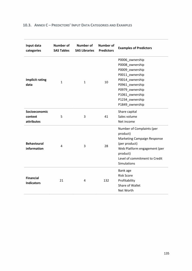
135
10.3. ANNEX C – PREDICTORS’ INPUT DATA CATEGORIES AND EXAMPLES
Input data
categories
Number of
SAS Tables
Number of
SAS Libraries
Number of
Predictors Examples of Predictors
Implicit rating
data 1 1 10
P0006_ownership
P0008_ownership
P0009_ownership
P0011_ownership
P0014_ownership
P0961_ownership
P0979_ownership
P1061_ownership
P1234_ownership
P1849_ownership
Socioeconomic
context
attributes
5 3 41
Share capital
Sales volume
Net income
Behavioural
information 4 3 28
Number of Complaints (per
product)
Marketing Campaign Response
(per product)
Web Platform engagement (per
product)
Level of commitment to Credit
Simulations
Financial
Indicators 21 4 132
Bank age
Risk Score
Profitability
Share of Wallet
Net Worth

Page | i