collaborative filtering recommendation techniques -...
TRANSCRIPT
Collaborative Filtering Recommendation Techniques
Yehuda Koren
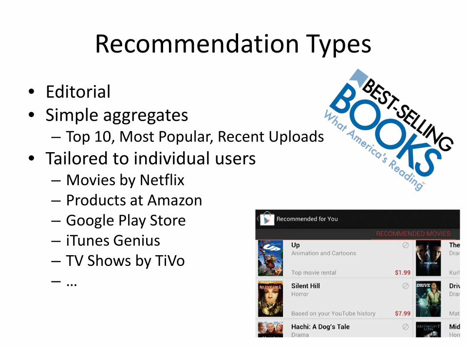
Recommendation Types
• Editorial • Simple aggregates
– Top 10, Most Popular, Recent Uploads • Tailored to individual users
– Movies by Netflix – Products at Amazon – Google Play Store – iTunes Genius – TV Shows by TiVo – …
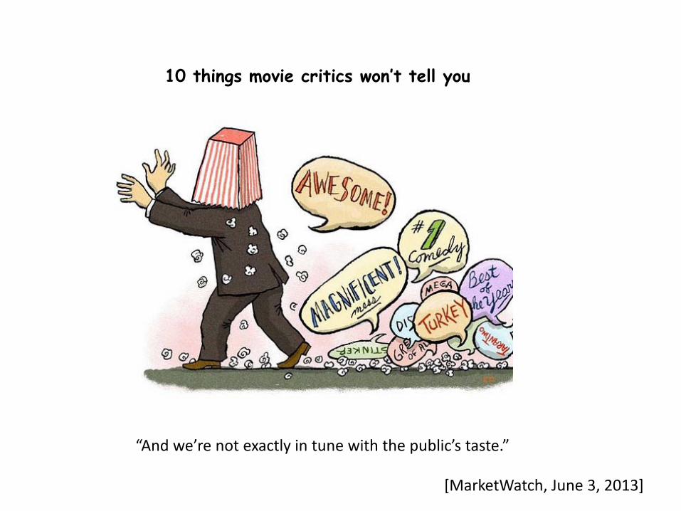
“And we’re not exactly in tune with the public’s taste.”
10 things movie critics won’t tell you
[MarketWatch, June 3, 2013]

4
Recommendation Process
Collecting “known” user-item ratings Extrapolate unknown ratings from
known ratings Estimate ratings for the items that have not
been seen by a user Recommend the items with the highest
estimated ratings to a user
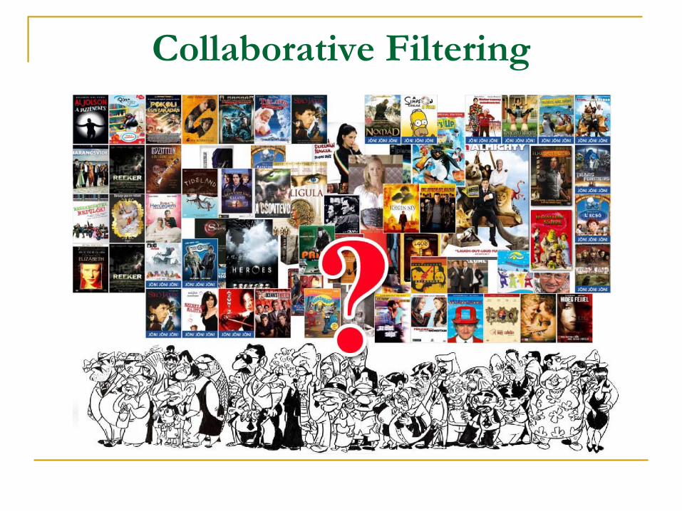
Collaborative Filtering

Collaborative filtering • Recommend items based on past transactions of many
users • Analyze relations between users and/or items • Specific data characteristics are irrelevant
– Domain-free: user/item attributes are not necessary – Can identify elusive aspects

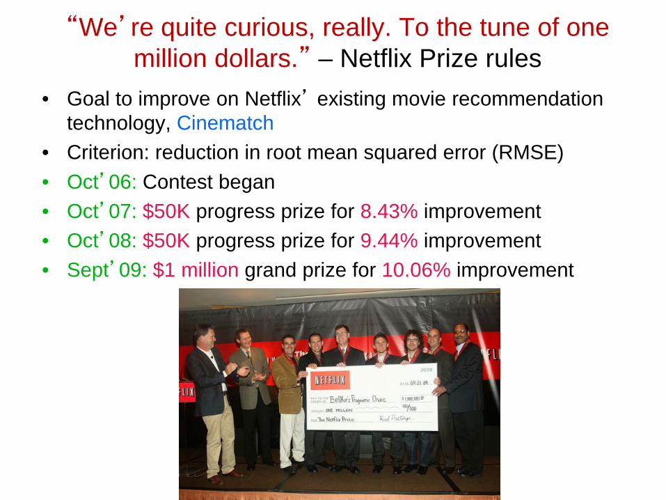
“We’re quite curious, really. To the tune of one million dollars.” – Netflix Prize rules
• Goal to improve on Netflix’ existing movie recommendation technology, Cinematch
• Criterion: reduction in root mean squared error (RMSE) • Oct’06: Contest began • Oct’07: $50K progress prize for 8.43% improvement • Oct’08: $50K progress prize for 9.44% improvement • Sept’09: $1 million grand prize for 10.06% improvement
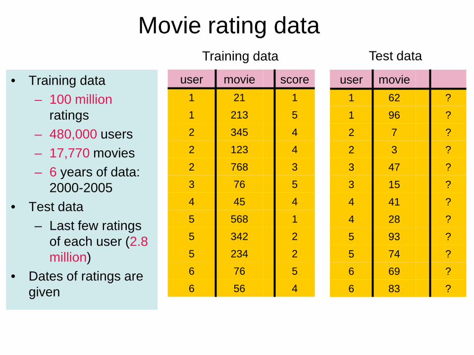
score movie user 1 21 1 5 213 1 4 345 2 4 123 2 3 768 2 5 76 3 4 45 4 1 568 5 2 342 5 2 234 5 5 76 6 4 56 6
movie user ? 62 1 ? 96 1 ? 7 2 ? 3 2 ? 47 3 ? 15 3 ? 41 4 ? 28 4 ? 93 5 ? 74 5 ? 69 6 ? 83 6
Training data Test data
Movie rating data
• Training data – 100 million
ratings – 480,000 users – 17,770 movies – 6 years of data:
2000-2005 • Test data
– Last few ratings of each user (2.8 million)
• Dates of ratings are given
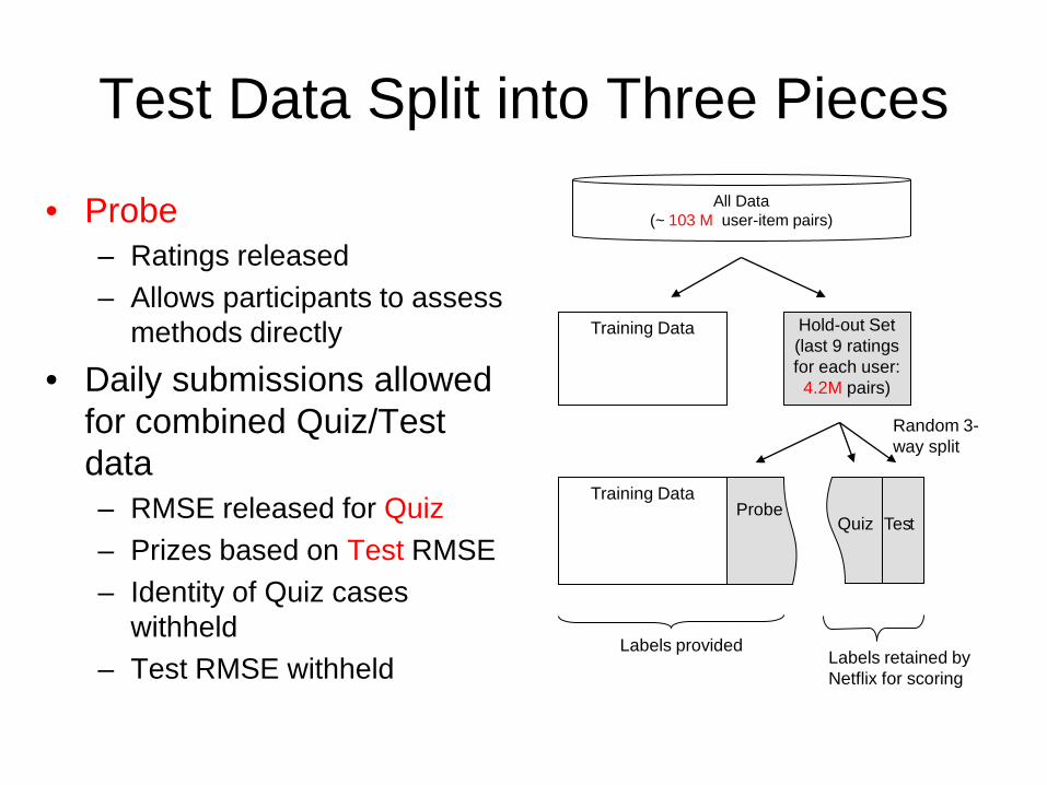
Test Data Split into Three Pieces
• Probe – Ratings released – Allows participants to assess
methods directly
• Daily submissions allowed for combined Quiz/Test data – RMSE released for Quiz – Prizes based on Test RMSE – Identity of Quiz cases
withheld – Test RMSE withheld
Training Data
Training Data
Hold-out Set (last 9 ratings for each user:
4.2M pairs)
All Data (~ 103 M user-item pairs)
Quiz
Test
Labels provided Labels retained by Netflix for scoring
Random 3-way split
Probe
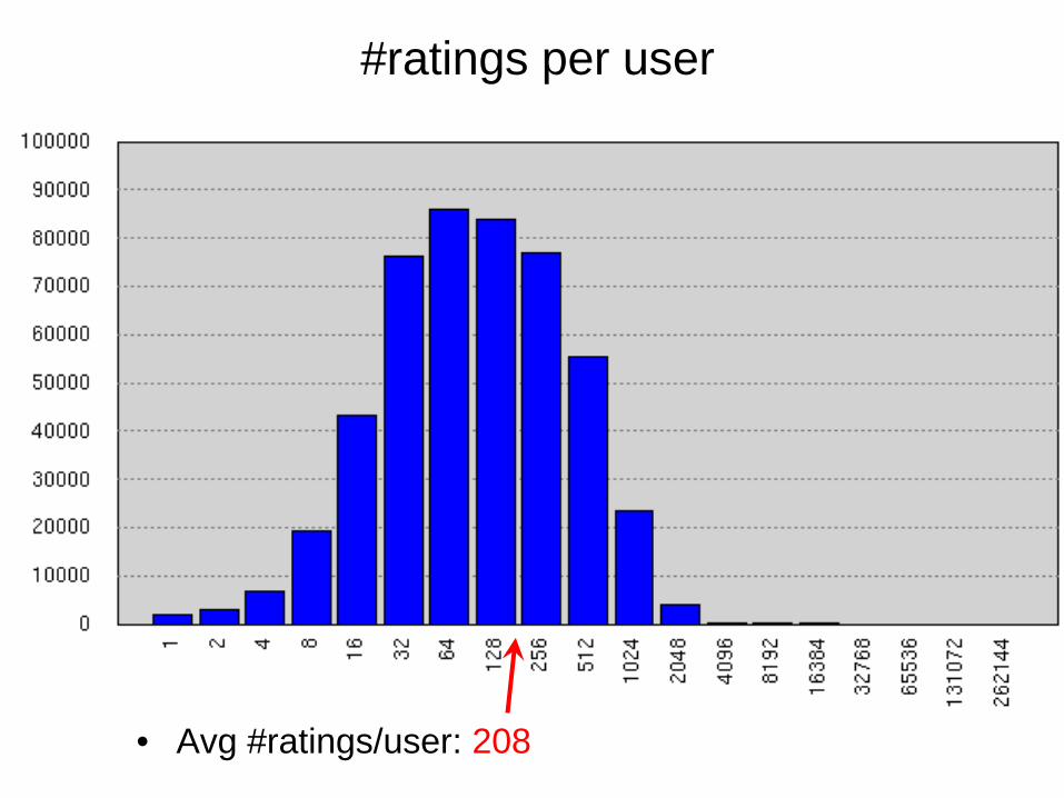
#ratings per user
• Avg #ratings/user: 208
12
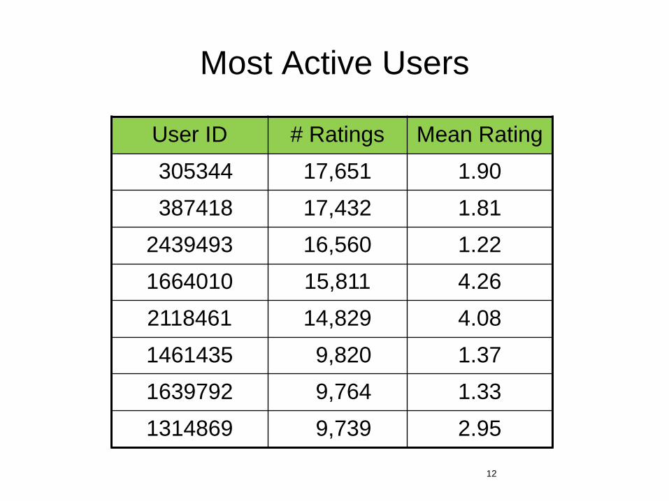
Most Active Users
User ID # Ratings Mean Rating 305344 17,651 1.90 387418 17,432 1.81 2439493 16,560 1.22 1664010 15,811 4.26 2118461 14,829 4.08 1461435 9,820 1.37 1639792 9,764 1.33 1314869 9,739 2.95
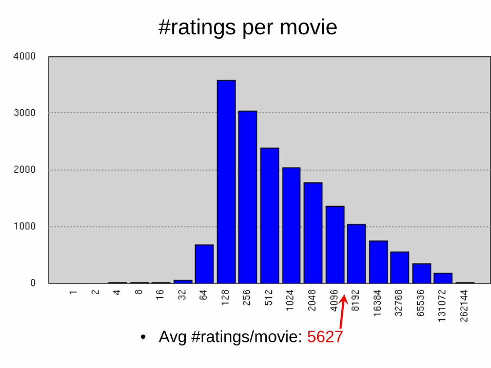
#ratings per movie
• Avg #ratings/movie: 5627
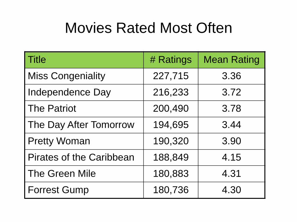
Movies Rated Most Often
Title # Ratings Mean Rating Miss Congeniality 227,715 3.36 Independence Day 216,233 3.72 The Patriot 200,490 3.78 The Day After Tomorrow 194,695 3.44 Pretty Woman 190,320 3.90 Pirates of the Caribbean 188,849 4.15 The Green Mile 180,883 4.31 Forrest Gump 180,736 4.30
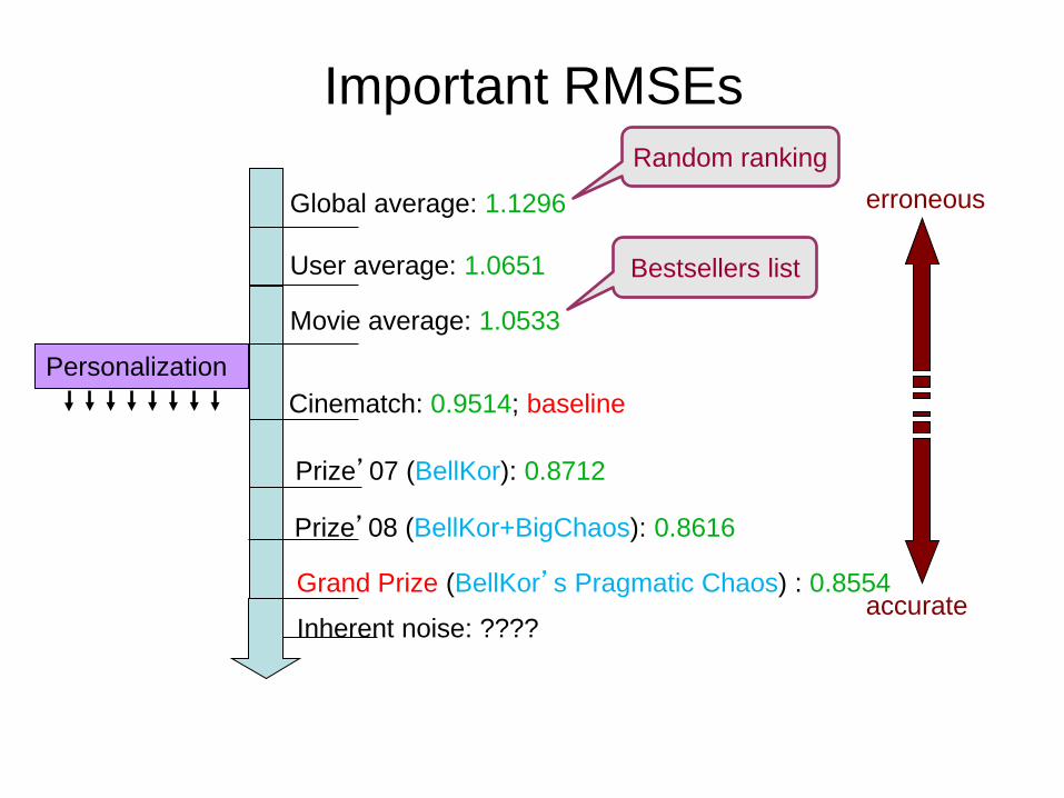
Important RMSEs
Prize’07 (BellKor): 0.8712
Cinematch: 0.9514; baseline
Movie average: 1.0533
User average: 1.0651
Global average: 1.1296
Inherent noise: ????
Personalization
erroneous
accurate
Prize’08 (BellKor+BigChaos): 0.8616
Grand Prize (BellKor’s Pragmatic Chaos) : 0.8554
Random ranking
Bestsellers list
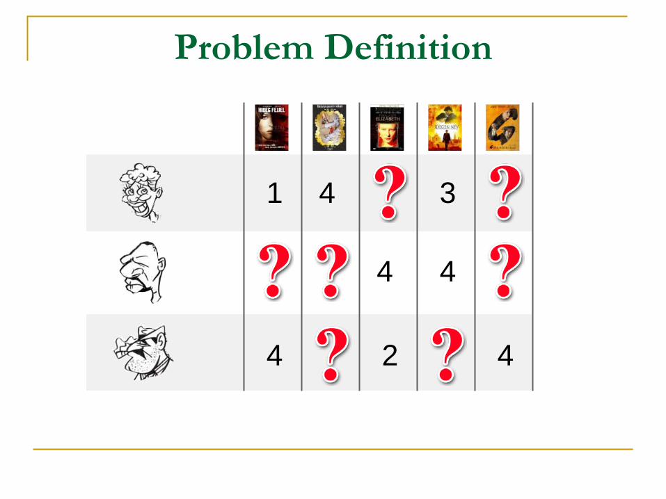
Problem Definition
1 4 3
4
4 4
4
2
#17,770
#3
#2
#1
Users➔ Items #480,000 #3 #2 #1
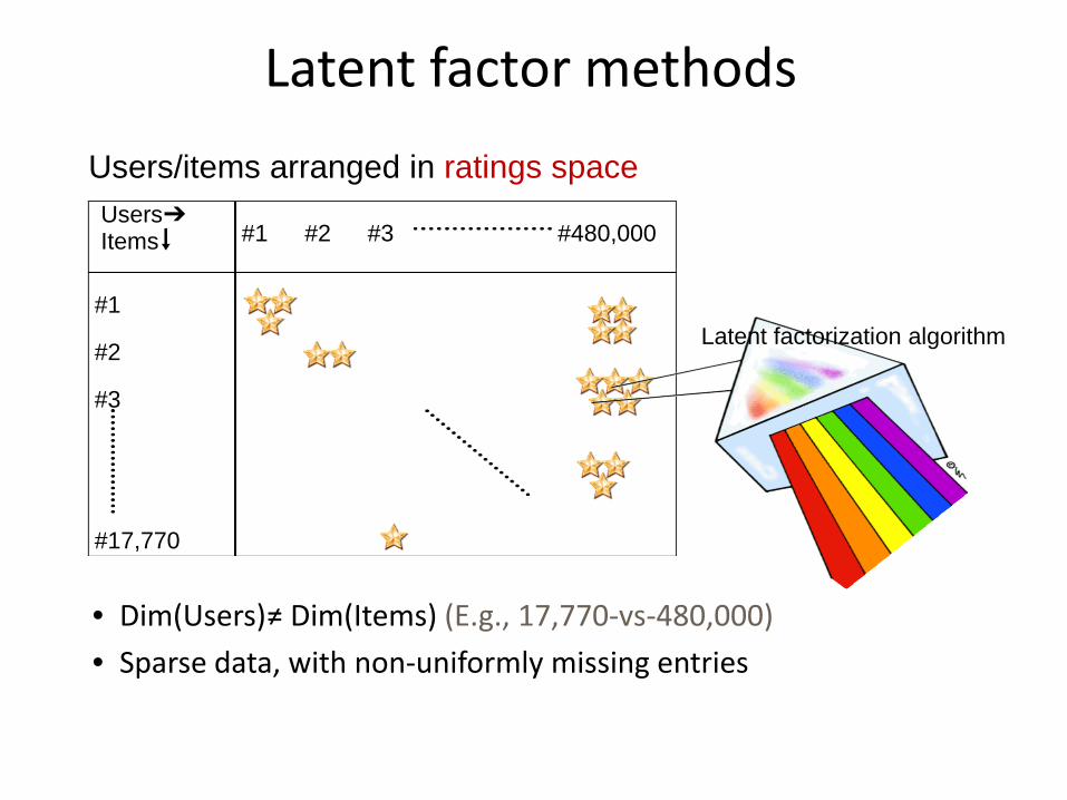
Users/items arranged in ratings space
Latent factorization algorithm
• Dim(Users)≠ Dim(Items) (E.g., 17,770-vs-480,000) • Sparse data, with non-uniformly missing entries
Latent factor methods
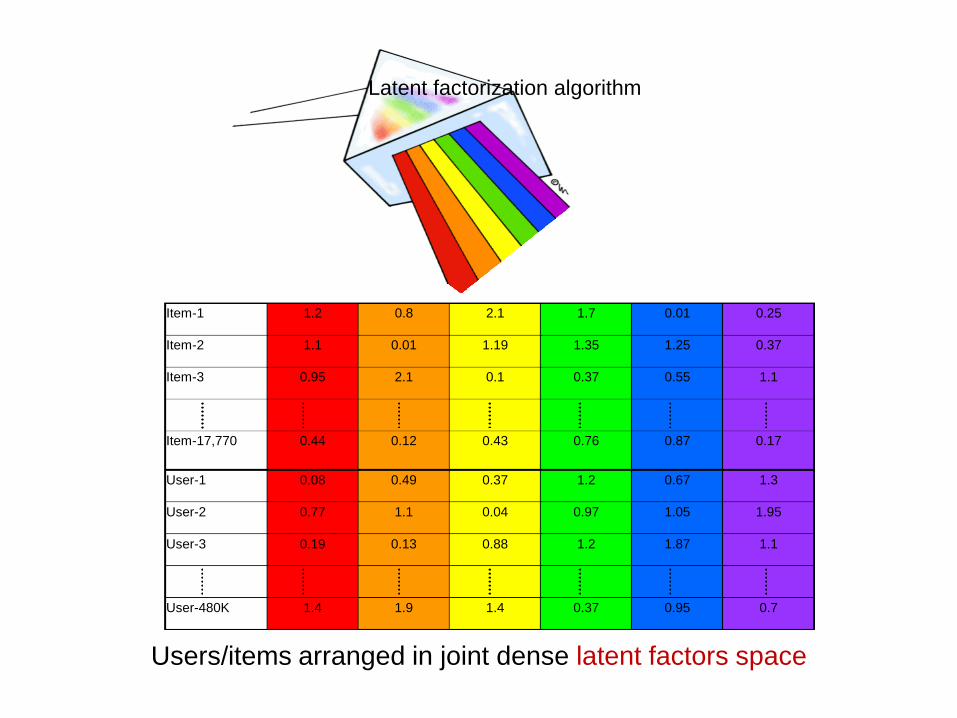
0.7 0.95 0.37 1.4 1.9 1.4 User-480K
1.1 1.87 1.2 0.88 0.13 0.19 User-3
1.95 1.05 0.97 0.04 1.1 0.77 User-2
1.3 0.67 1.2 0.37 0.49 0.08 User-1
0.17 0.87 0.76 0.43 0.12 0.44 Item-17,770
1.1 0.55 0.37 0.1 2.1 0.95 Item-3
0.37 1.25 1.35 1.19 0.01 1.1 Item-2
0.25 0.01 1.7 2.1 0.8 1.2 Item-1
Latent factorization algorithm
Users/items arranged in joint dense latent factors space
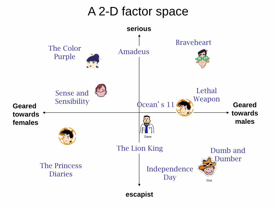
Geared towards females
Geared towards males
serious
escapist
The Princess Diaries
The Lion King
Braveheart
Lethal Weapon
Independence Day
Amadeus The Color Purple
Dumb and Dumber
Ocean’s 11
Sense and Sensibility
Gus
Dave
A 2-D factor space
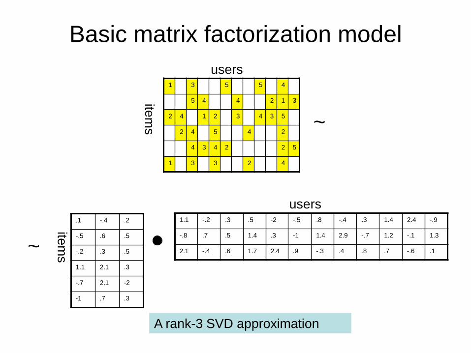
Basic matrix factorization model
4 5 5 3 1
3 1 2 4 4 5
5 3 4 3 2 1 4 2
2 4 5 4 2
5 2 2 4 3 4
4 2 3 3 1
items
.2 -.4 .1
.5 .6 -.5
.5 .3 -.2
.3 2.1 1.1
-2 2.1 -.7
.3 .7 -1
-.9 2.4 1.4 .3 -.4 .8 -.5 -2 .5 .3 -.2 1.1
1.3 -.1 1.2 -.7 2.9 1.4 -1 .3 1.4 .5 .7 -.8
.1 -.6 .7 .8 .4 -.3 .9 2.4 1.7 .6 -.4 2.1
~
~
items
users
users
A rank-3 SVD approximation
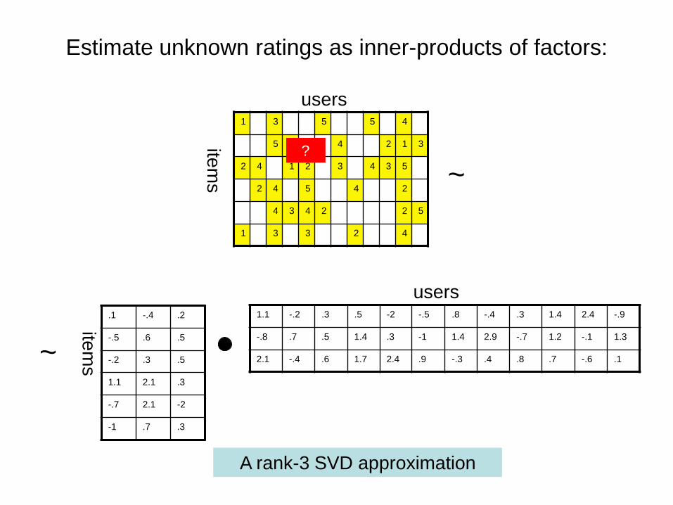
Estimate unknown ratings as inner-products of factors:
4 5 5 3 1
3 1 2 4 4 5
5 3 4 3 2 1 4 2
2 4 5 4 2
5 2 2 4 3 4
4 2 3 3 1
items
.2 -.4 .1
.5 .6 -.5
.5 .3 -.2
.3 2.1 1.1
-2 2.1 -.7
.3 .7 -1
-.9 2.4 1.4 .3 -.4 .8 -.5 -2 .5 .3 -.2 1.1
1.3 -.1 1.2 -.7 2.9 1.4 -1 .3 1.4 .5 .7 -.8
.1 -.6 .7 .8 .4 -.3 .9 2.4 1.7 .6 -.4 2.1
~
~
items
users
A rank-3 SVD approximation
users
?
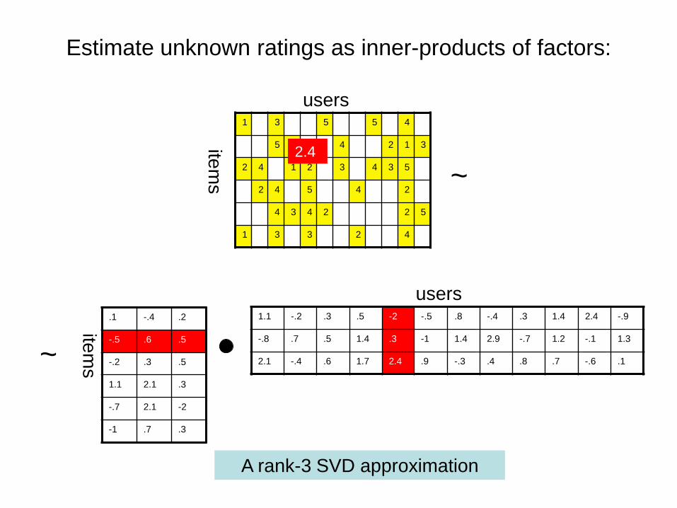
Estimate unknown ratings as inner-products of factors:
4 5 5 3 1
3 1 2 4 4 5
5 3 4 3 2 1 4 2
2 4 5 4 2
5 2 2 4 3 4
4 2 3 3 1
items
.2 -.4 .1
.5 .6 -.5
.5 .3 -.2
.3 2.1 1.1
-2 2.1 -.7
.3 .7 -1
-.9 2.4 1.4 .3 -.4 .8 -.5 -2 .5 .3 -.2 1.1
1.3 -.1 1.2 -.7 2.9 1.4 -1 .3 1.4 .5 .7 -.8
.1 -.6 .7 .8 .4 -.3 .9 2.4 1.7 .6 -.4 2.1
~
~
items
users
2.4
A rank-3 SVD approximation
users
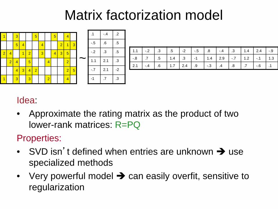
Matrix factorization model 4 5 5 3 1
3 1 2 4 4 5
5 3 4 3 2 1 4 2
2 4 5 4 2
5 2 2 4 3 4
4 2 3 3 1
.2 -.4 .1
.5 .6 -.5
.5 .3 -.2
.3 2.1 1.1
-2 2.1 -.7
.3 .7 -1
-.9 2.4 1.4 .3 -.4 .8 -.5 -2 .5 .3 -.2 1.1
1.3 -.1 1.2 -.7 2.9 1.4 -1 .3 1.4 .5 .7 -.8
.1 -.6 .7 .8 .4 -.3 .9 2.4 1.7 .6 -.4 2.1 ~
Idea: • Approximate the rating matrix as the product of two
lower-rank matrices: R=PQ Properties: • SVD isn’t defined when entries are unknown use
specialized methods • Very powerful model can easily overfit, sensitive to
regularization
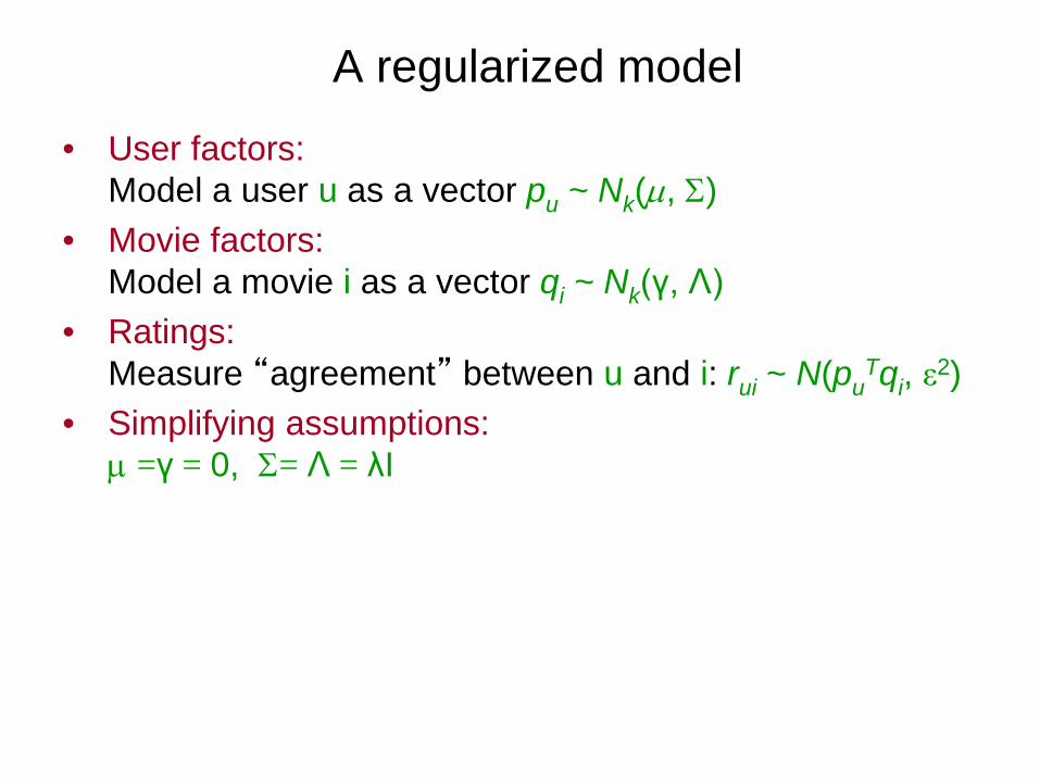
A regularized model
• User factors: Model a user u as a vector pu ~ Nk(µ, Σ)
• Movie factors: Model a movie i as a vector qi ~ Nk(γ, Λ)
• Ratings: Measure “agreement” between u and i: rui ~ N(pu
Tqi, ε2) • Simplifying assumptions:
µ =γ = 0, Σ= Λ = λI
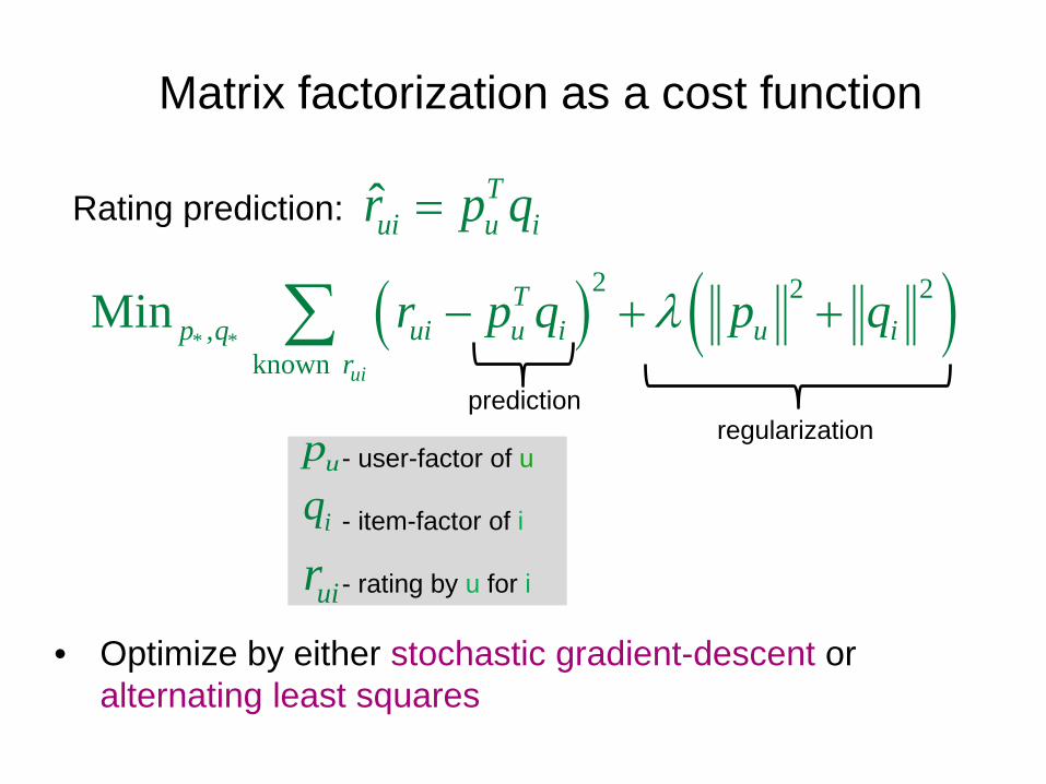
Matrix factorization as a cost function
ˆ Tui u ir p q=
regularization - user-factor of u - item-factor of i
- rating by u for i uir
iqup
• Optimize by either stochastic gradient-descent or alternating least squares
prediction
( ) ( )* *
2 2 2,
knownMin
ui
Tp q ui u i u i
rr p q p qλ− + +∑
Rating prediction:

Alternating Least Squares (ALS)
• Alternate between solving two least squares (Ridge regression) problems:
R ≈ PQ • Fix item factors (Q) and find P by regressing R on Q • Fix user factors (P) and find Q by regressing R on P • Make a few sweeps…
( ) ( )* *
2 2 2,
knownMin
ui
Tp q ui u i u i
rr p q p qλ− + +∑
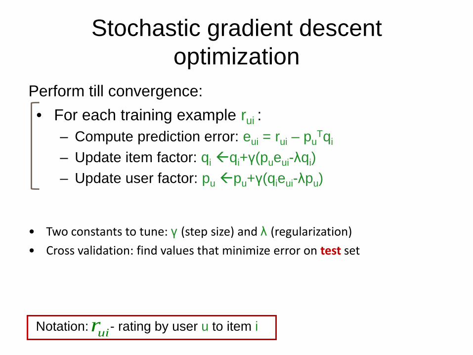
Stochastic gradient descent optimization
• For each training example rui : – Compute prediction error: eui = rui – pu
Tqi
– Update item factor: qi qi+γ(pueui-λqi) – Update user factor: pu pu+γ(qieui-λpu)
Perform till convergence:
• Two constants to tune: γ (step size) and λ (regularization) • Cross validation: find values that minimize error on test set
Notation: - rating by user u to item i uir
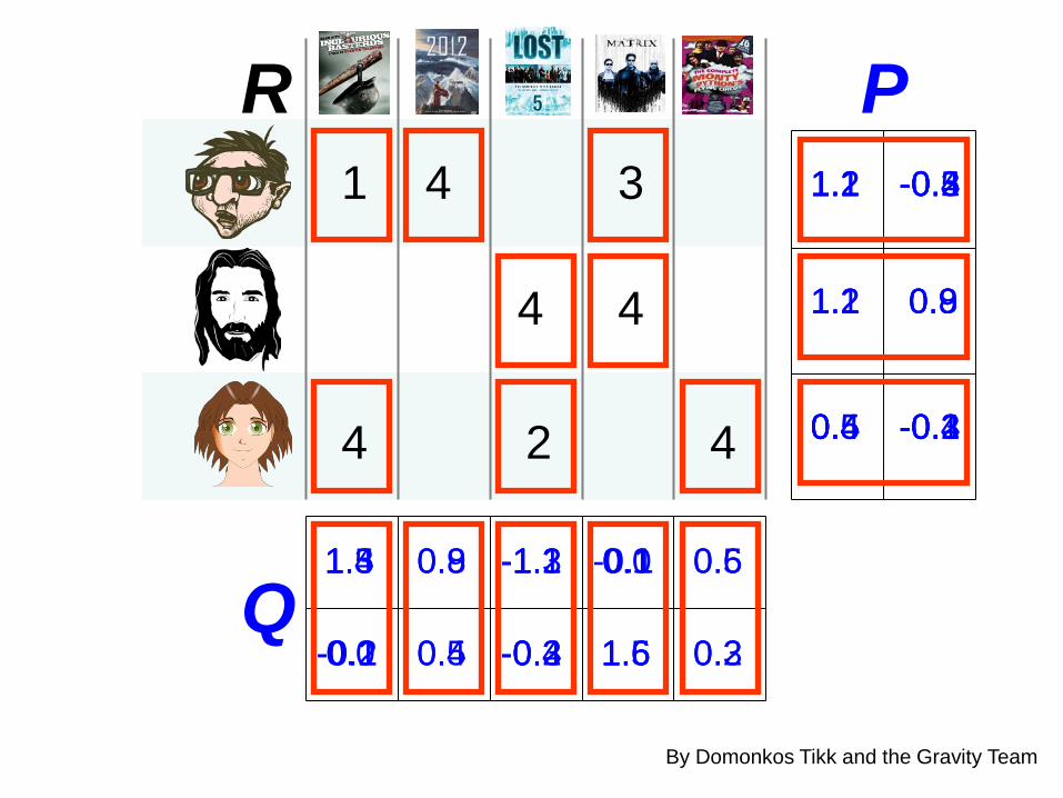
1 4 3
4
4 4
4
2
1.4
-0.2
0.8
0.5
-1.3
-0.4 1.6
-0.1 0.5
0.3
1.2 -0.5 1.1 -0.4
1.2 0.9
0.4 -0.4
1.2 -0.3
1.3
-0.1
0.9
0.4
1.1 -0.2
1.5
0.0
1.1 0.8
-1.2
-0.3
1.2 0.9
1.6
0.1 1.5
0.0
0.5 -0.3
-1.1
-0.2
0.4 -0.2 0.5 -0.1
0.6
0.2
P
Q
R
By Domonkos Tikk and the Gravity Team

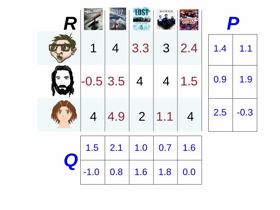
1 4 3
4
4 4
4
2
1.5
-1.0
2.1
0.8
1.0
1.6 1.8
0.7 1.6
0.0
1.4 1.1
0.9 1.9
2.5 -0.3
P
Q
R 3.3 2.4
-0.5 3.5 1.5
1.1 4.9
Data normalization
• Most variability in observed data is driven by user-specific and item-specific effects, regardless of user-item interaction
• Examples: – Some movies are systematically rated higher – Some movies were rated by users that tend to rate low – Ratings change along time
• Data must be adjusted to account for these main effects • This stage requires most insights into the nature of the data • Can make a big difference…
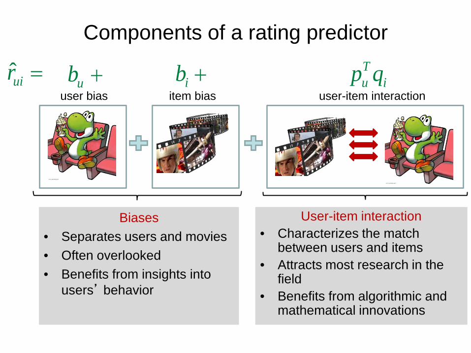
Components of a rating predictor
user-item interaction item bias user bias
User-item interaction • Characterizes the match
between users and items • Attracts most research in the
field • Benefits from algorithmic and
mathematical innovations
Biases • Separates users and movies • Often overlooked • Benefits from insights into
users’ behavior
ub + ib + Tu ip quir =
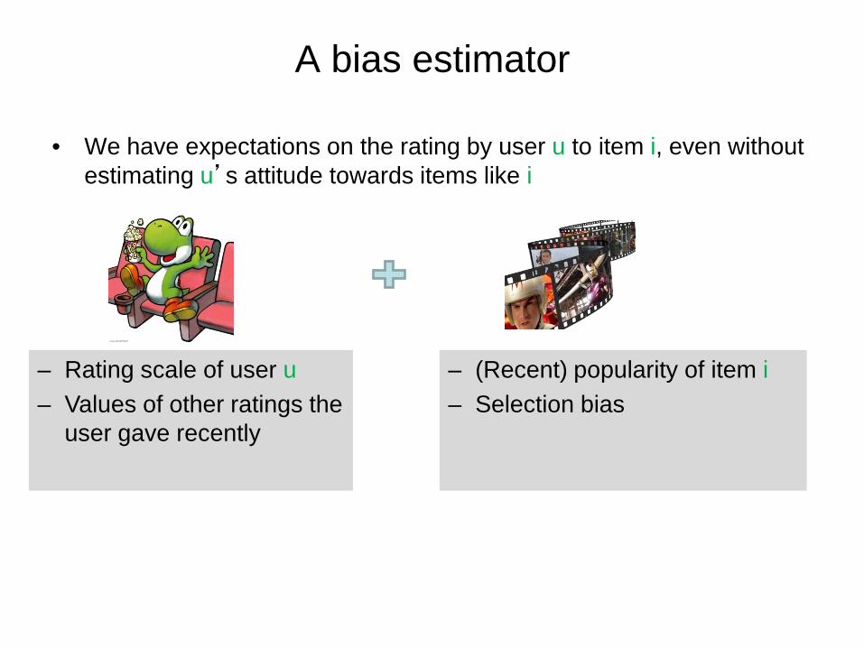
A bias estimator
• We have expectations on the rating by user u to item i, even without estimating u’s attitude towards items like i
– Rating scale of user u – Values of other ratings the
user gave recently
– (Recent) popularity of item i – Selection bias
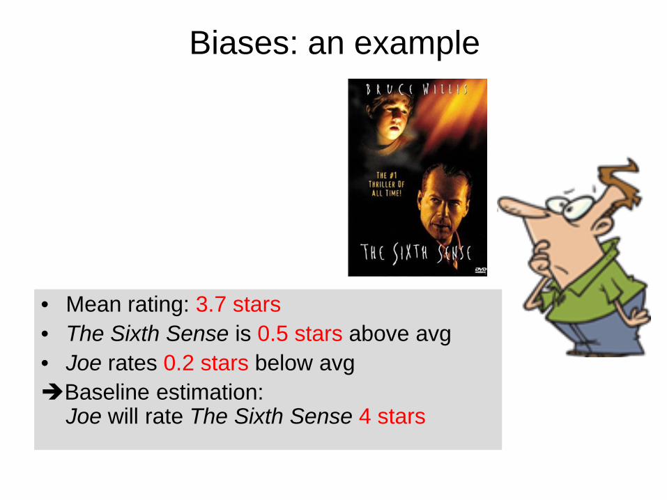
Biases: an example
• Mean rating: 3.7 stars • The Sixth Sense is 0.5 stars above avg • Joe rates 0.2 stars below avg Baseline estimation:
Joe will rate The Sixth Sense 4 stars
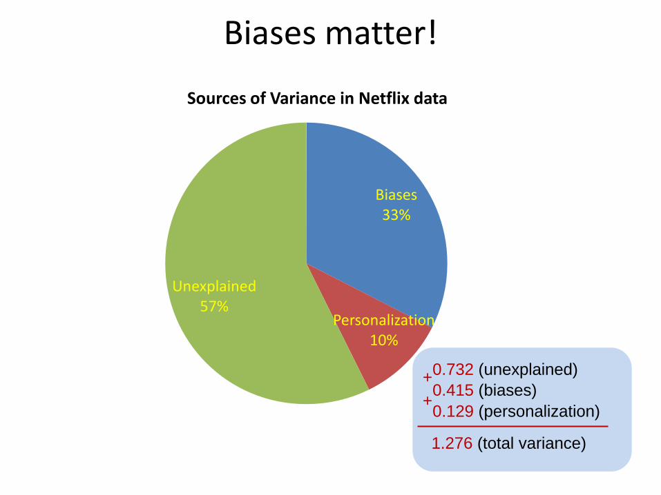
Biases 33%
Personalization 10%
Unexplained 57%
Sources of Variance in Netflix data
1.276 (total variance)
0.732 (unexplained) 0.415 (biases) 0.129 (personalization)
+ +
Biases matter!
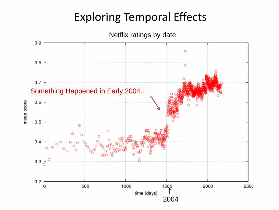
Exploring Temporal Effects
2004
Netflix ratings by date
Something Happened in Early 2004…
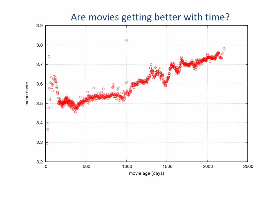
Are movies getting better with time?
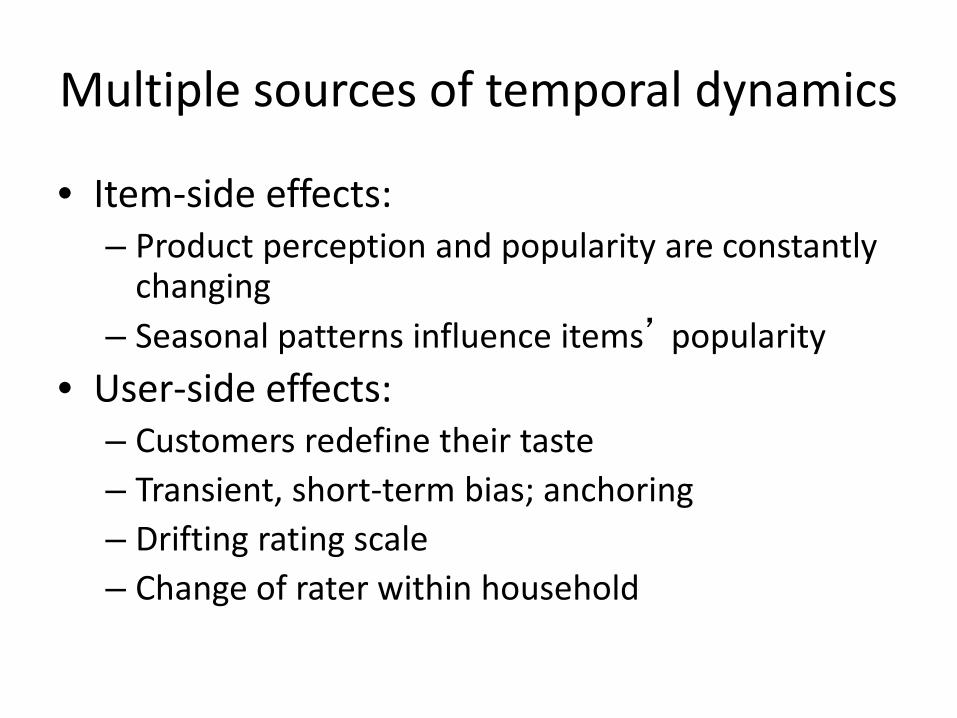
Multiple sources of temporal dynamics
• Item-side effects: – Product perception and popularity are constantly
changing – Seasonal patterns influence items’ popularity
• User-side effects: – Customers redefine their taste – Transient, short-term bias; anchoring – Drifting rating scale – Change of rater within household
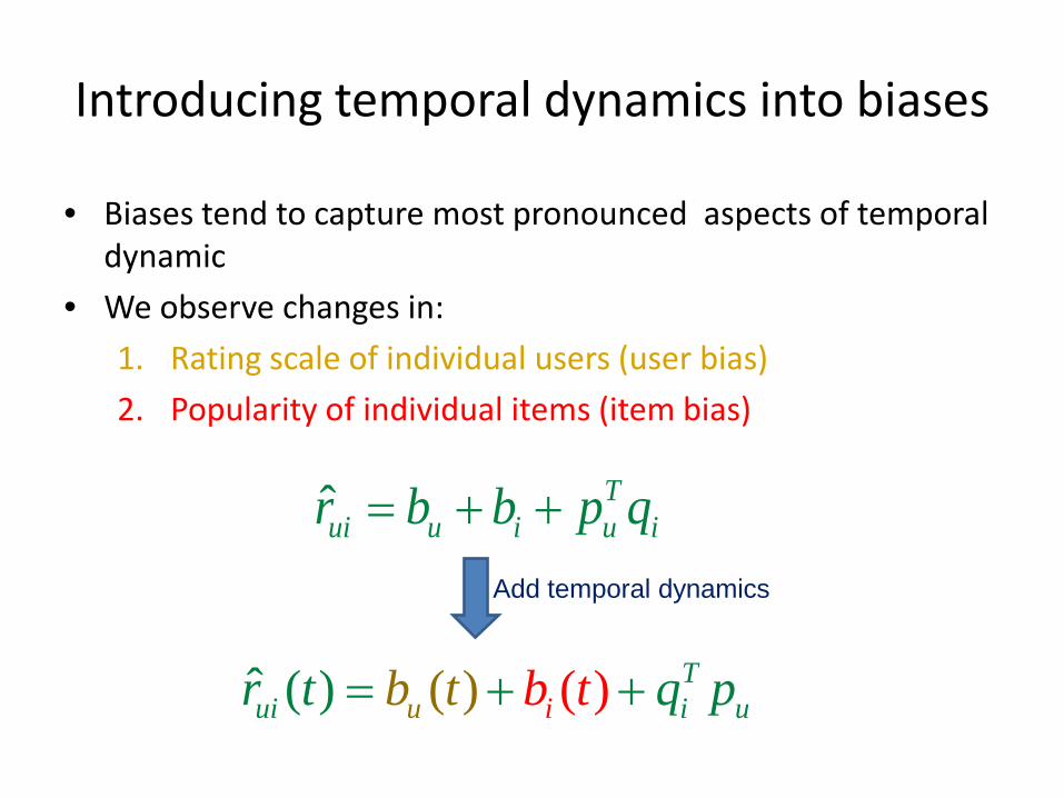
Introducing temporal dynamics into biases
• Biases tend to capture most pronounced aspects of temporal dynamic
• We observe changes in: 1. Rating scale of individual users (user bias) 2. Popularity of individual items (item bias)
( )ˆ (( )) Tu i i uui b b ptt tr q= + +
ˆ Tui u i u ir b b p q= + +
Add temporal dynamics

General Lessons and Experience

• 1.4M predictions are split into 10 equal bins based on #ratings per user
Some users are more predictable…
0.7
0.75
0.8
0.85
0.9
0.95
1
12 24.4 38.1 55.4 80.9 119.4 176.5 264.8 420.9 918.5
RMSE vs. #Ratings

Ratings are not given at random!
Marlin, Zemel, Roweis, Slaney, “Collaborative Filtering and the Missing at Random Assumption” UAI 2007
Yahoo! survey answers Yahoo! music ratings Netflix ratings
Distribution of ratings
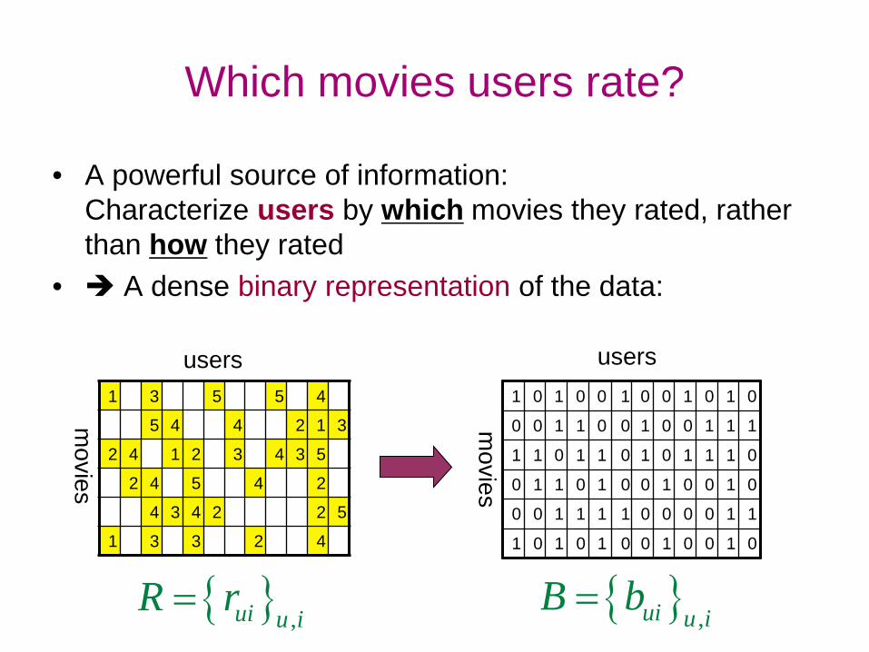
• A powerful source of information: Characterize users by which movies they rated, rather than how they rated
• A dense binary representation of the data:
4 5 5 3 1
3 1 2 4 4 5
5 3 4 3 2 1 4 2
2 4 5 4 2
5 2 2 4 3 4
4 2 3 3 1
users
movies
0 1 0 1 0 0 1 0 0 1 0 1
1 1 1 0 0 1 0 0 1 1 0 0
0 1 1 1 0 1 0 1 1 0 1 1
0 1 0 0 1 0 0 1 0 1 1 0
1 1 0 0 0 0 1 1 1 1 0 0
0 1 0 0 1 0 0 1 0 1 0 1
users m
ovies
Which movies users rate?
{ } ,ui u iR r= { } ,ui u i
B b=

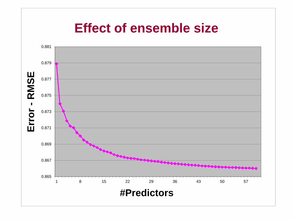
The Wisdom of Crowds (of Models)
• All models are wrong; some are useful – G. Box – Some miss strong “local” relationships, e.g., among sequels – Others miss cumulative effect of many small signals – Each complements the other
• Our best entry during Year 1 was a linear combination of 107 sets of predictions
• Our final solution was a linear blend of over 700 prediction sets – Many variations of model structure and parameter settings
• Mega blends are not needed in practice – A handful of simple models achieves 90% of the improvement of
the full blend
0.865
0.867
0.869
0.871
0.873
0.875
0.877
0.879
0.881
1 8 15 22 29 36 43 50 57
Erro
r - R
MSE
#Predictors
Effect of ensemble size
4 5 5 3 1
3 1 2 4 4 5
5 3 4 3 2 1 4 2
2 4 5 4 2
5 2 2 4 3 4
4 2 3 3 1
3 4 3 2 1
4 5 4
2 4 3 4
3 2 5
2 4
Yehuda Koren Google