Collaborators:

Ulrich BroseCarol BlanchetteJennifer Dunne

Sonia KefiNeo MartinezBruce Menge

Sergio NavarreteOwen Petchey

Philip StarkRich Williams

…

Predictability

Predict

Biodiversity

Prediction

Biodiversity

Changes in Focal Species

….add bit about yosemite toad or mt yellow legged frog

How can we predict the consequences of species loss in complex ecosystems?

Little Rock Lake Food Web (Martinez 1991)

1 degree

How can we predict the consequences of species loss in complex ecosystems?

Little Rock Lake Food Web (Martinez 1991)

2 degrees

How can we predict the consequences of species loss in complex ecosystems?

Little Rock Lake Food Web (Martinez 1991)

3 degrees

Williams et al. PNAS 2002

How can we predict the consequences of species loss in complex ecosystems?

Little Rock Lake Food Web (Martinez 1991)

Complex

Complicated

some hope

metabolism

<1>

everything needs energy to stay alive

<2>

BIG things need more energy than small things

<2>

BIG things need more energy than small things( )3/4

allometric scaling of metabolism with body size

Feeding is Universal

Food Webs are the foundation of Ecological Networks

Body Size should predict the strength of interactions in food webs

Feeding is Universal

Universal ≠ The Only Thing

Ubiquitous≠ The Only Thing

non-metabolic interactions

R. Donovan

Question

can we explain with body size (metabolism)?

ALL interaction strengths

can we explain with body size (metabolism)?

ALL interaction strengths

can we explain with body size (metabolism)?

WHAT

can we explain with body size (metabolism)?

WHAT NOT

.

repeat it

can we explain with body size (metabolism)?

ALL interaction strengths

can we explain with body size (metabolism)?

WHAT

can we explain with body size (metabolism)?

WHAT NOT

abun

danc

e,in

tera

ction

str

engt

h,et

c.

?

abun

danc

e,in

tera

ction

str

engt

h,et

c.

feeding,body size,

metabolism,etc.

abun

danc

e,in

tera

ction

str

engt

h,et

c.

feeding,body size,

metabolism,etc.

can wedescribe a metabolic baseline of interactions

in complex networks?

can wedetrend metabolism

in complex networks?

Brose et al. 2005 EcologyBrose et al. 2006 EcologyPetchey et al. 2008 PNAS

Body Size also influences Food Web Structure

if each link obeys allometric rulesare those rules preserved at the network scale?

if each link obeys allometric ruleswill body size predict

the effect of species loss in the network?

does more complex = more complicated?

Approach

Simulation Results

Real World

Approach:

<1>

Simulate species dynamics in a wide variety of networks

stochastic variation instructural and dynamic

parameters

Approach:

<2>

all feeding links governed by (body size)¾

Approach:

<3>

delete each species and measure effects on all others

Approach:

<4>

Track variation for each simulation

interaction strengthsnetwork level structureneighborhood structure

species attributeslink attributes

Approach:

<5>

mine the variability for what best explains interaction strengths

The Model

The Modelscoupled

<1> Food Web Structure: Niche Model

(Williams and Martinez 2000)

<2> Predator-Prey Interactions: Bio-energetic Model

(Yodzis and Innes 1992, Brose et al. 2005, 2006 Eco Letts)

<3> Plant population dynamics: Plant-Nutrient Model

(Tilman 1982, Huisman and Weissing 1999)

consumersj

jijijjresourcesj

ijiiiii eFyBxFyBxBxB /'

Bioenergetic Predator-Prey Dynamics

Biomassi at time t

Biomass of each species (i) at time (t) is balance of1. gain from consuming prey species 2. loss to being consumed by other species 3. loss to metabolism

mass-specific metabolic rate

max metabolic-specific ingestion rate

Functional Response

assimilationefficiency

Bioenergetic Predator-Prey Dynamics

consumersj

jijijjresourcesj

ijiiiii eFyBxFyBxBxB /'

xi, yi scale with body size(body size correlated with web structure)

# Prey

Cons

umpti

on

Nutrient-DependentGrowth of Plants

Bioenergetic Predator-Prey Dynamics(Plants)

consumersj

jijijjiiiiii eFyBxBxBGrB /'

mass-specificgrowth rate metabolic loss loss to herbivores

ri, xj, y scale with body size

Nutrient-Dependent Growth of Plants

Growth determined by most limiting Nutrient

plantgrowth rate

Concentration of Nutrientsdetermined by

SupplyTurnover

Consumption

Half saturation conc. for uptake of that Nutrient

)(,)(22

2

11

1 tBNK

N

NK

NMINNG i

iii

Generate a food web (Niche Model)

Calculate trophic level for each species

Apply plant-nutrient model to plants, predator-prey model to rest.

Assign body sizes based on trophic level (mean pred: prey ratio = 10)

Run simulation with each species deleted individually to generate a complete removal matrix

Repeat for all species and for 600 Niche Model webs

R

T

Removed Species

Target Species

R

T

X+

R

T

R

T

X-

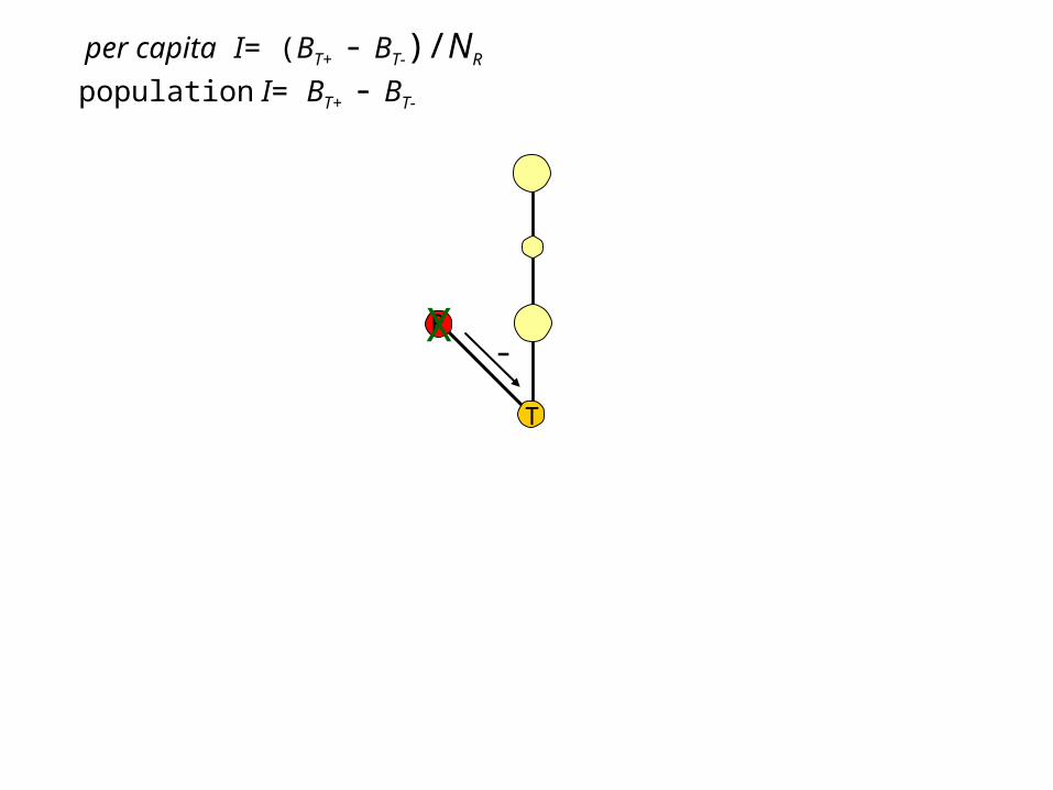
per capita I= (BT+ - BT-)/NR

population I= BT+ - BT-

R

T

X-

per capita I= (BT+ - BT-)/NR

population I= BT+ - BT-

R

T

X-

per capita I= (BT+ - BT-)/NR

population I= BT+ - BT-

R

T

X-

per capita I= (BT+ - BT-)/NR

population I= BT+ - BT-

R

T

X ?

T

per capita I= (BT+ - BT-)/NR

population I= BT+ - BT-

R

T

X 1° Consumers

2° Consumers

3° Consumers

1° Prey

2° Prey

3° Prey

?

T

per capita I= (BT+ - BT-)/NR

population I= BT+ - BT-

R

T

X 1° Consumers

2° Consumers

3° Consumers

1° Prey

2° Prey

3° Prey

?

T

per capita I= (BT+ - BT-)/NR

population I= BT+ - BT-

K

D S1

NK1

K = Keystone consumerNK = Non-Keystone consumer

D = Dominant basal speciesS = Subordinate basal species

R = ResourceR1 R2

S1

S2

K

D S1

NK1

+

Keystone Present

R1 R2

Consumption

Resource competition

Indirect Facilitation

S1

S2

K

D S1

NK1

+

Keystone Present

R1 R2Increased Resources

Consumption

Resource competition

Indirect Facilitation

S1

S2

K

D S1

NK1

Sn

Other Competitors

+

Keystone Present

R1 R2

Consumption

Resource competition

Indirect Facilitation

S1

K

D S1

NK1

Secondary Consumers

+

R1 R2

NK2n

Consumption

Resource competition

Indirect Facilitation

S1

S2

K

D S1

NK1

NK3nTertiary Consumers

+

Secondary Consumers

R1 R2

NK2n

Consumption

Resource competition

Indirect Facilitation

S1

S2

K

D S1

NK1

NK2n

NK3nTertiary Consumers

+

Secondary Consumers

R1 R2

and so on… NK4n

S1

K

D S1

+

S2

Bottom up

Top down

Horizontal

add noise

track the consequences of that noise

add noise:

<1>

Web Structuresize, connectance, architecture

add noise:

<2>

Animal Attributes metabolic and max consumption rate,

pred-prey body size ratiofunctional response type

predator interference

add noise:

<3>

Plant Attributesgrowth rate

half saturation concentrations

track:

90 predictors to explain

variation in the strengths of

254,032 interactions among

12,116 species in

600 webs

track:

<1>Global network structure

<2>Species attributes of R and T

<3>Local network structure around each R and T

<4>Attributes of the interaction

prey predatorpredator prey

+

-

R

T

R T

attributes of the interaction+-

shortest path = 2 degrees

2 degree paths: +, +, -prey predator

predator prey

+

-

R

T

R T+-

attributes of the interaction

shortest path = 2 degrees

2 degree paths: +, +, -3 degree paths: +, +, +, -prey predator

predator prey

+

-

R

T

R T+-

attributes of the interaction

shortest path = 2 degrees

2 degree paths: +, +, -3 degree paths: +, +, +, -4 degree paths: -

prey predatorpredator prey

+

-

R

T

R T+-

sign shortest path = +1sign next shortest path = +2un-weighted sum (shortest + next shortest) = +3weighted sum (shortest + (next shortest / 2)) = +2

attributes of the interaction

-2

0

2

4

6

8

Log

(Bod

y M

ass)

1 2 3 4 5 6 7 8

Trophic Level

Body Size and Food Web Structure

R2 = 0.90Slope = 0.74

Lo

g (

per

ca

pit

a co

nsu

mp

tio

n)

-12

-9

-6

-3

0

3

6

9

PC

Lin

IS)

-4 -2 0 2 4 6 8 10log (SR mass)

Log (R body mass)

Each Feeding Interaction Scales with (Body Size)3/4

R

T

R2 = 0.90Slope = 0.74

Lo

g (

per

ca

pit

a co

nsu

mp

tio

n)

Per Capita Linear Interaction Strength

-12

-9

-6

-3

0

3

6

9

PC

Lin

IS)

-4 -2 0 2 4 6 8 10log (SR mass)

Log (R body mass)

R

T

= Per Capita Removal Interaction Strength?

-12

-9

-6

-3

0

3

6

9

log

(|D

iff P

C|)

-4 -2 0 2 4 6 8 10log (SR mass)

Lo

g |

per

ca

pit

a I|

R2 = 0.32Slope = 0.74

Log (R body mass)

Per Capita Removal Interaction Strength

R

T

-12

-9

-6

-3

0

3

6

9

log

(|D

iff P

C|)

-4 -2 0 2 4 6 8 10log (SR mass)

Lo

g |

per

ca

pit

a I|

R2 = 0.14Slope = 1.3

Log (R body mass)

Per Capita Removal Interaction Strength

R

T

-12

-9

-6

-3

0

3

6

9

log

(|D

iff P

C|)

-4 -2 0 2 4 6 8 10log (SR mass)

Log (R body mass)

Lo

g |

per

ca

pit

a I|

R2 = 0.45Slope = 1.4

Per Capita Removal Interaction Strength

R

T

-6

-3

0

3

6

Res

idua

ls

log

(abs

PC

)

-15 -12 -9 -6 -3 0log (TS biom)

-12

-9

-6

-3

0

3

6

9

log

(|D

iff P

C|)

-4 -2 0 2 4 6 8 10log (SR mass)

Log (R body mass)

Lo

g |

per

ca

pit

a I|

Per Capita Interaction Strength

Low R BiomassHigh R Biomass

Res

idu

als

Log (T biomass)

Per Capita Removal Interaction Strength

R

T

Predicted by:Log (T biomass) +Log (R biomass) +Log (R body mass)

Lo

g |

per

ca

pit

a I|

Per Capita Interaction Strength

-12

-9

-6

-3

0

3

6

9

log

(|D

iff P

C|)

-10 -8 -6 -4 -2 0 2 4 6 8Pred Formula log (|Diff PC|)

R2 = 0.88

R

T

population I

(population interaction strength)

population I

(total effect on T of removing R)

Classification and Regression Trees (CART)on log transformed |Interaction Strengths|

best predictors of absolute magnitude of log(population I)

T biomassR biomass

(Degrees Separated)

of the 90 variables tracked

R2 = 0.65

-12

-9

-6

-3

0

log

(|D

iff T

E|)

-12 -9 -6 -3 0log (TS biom)

Lo

g |

po

pu

lati

on

I|

Log (T biomass)

-12

-9

-6

-3

0

log

(|D

iff T

E|)

-12 -9 -6 -3 0log (TS biom)

Low R BiomassHigh R Biomass

Log (T biomass)

Lo

g |

po

pu

lati

on

I|

R2 = 0.65

Sign (strong interactions)

0.00

0.25

0.50

0.75

1.00

-1 0 1

-1

1

≤ -1 ≥ 1

Weighted Sum Path Signs

Pro

po

rtio

n O

bse

rved

0.00

0.25

0.50

0.75

1.00

-1 0 1

-1

1

Sign (weak interactions)

≤ -1 ≥ 1

Weighted Sum Path Signs

positive

negative

-18

-15

-12

-9

-6

-3

0

log

(abs

TE

)

-15 -12 -9 -6 -3 0log (TS biom)

-6

-3

0

3

6

Res

idua

ls

log

(abs

PC

)-15 -12 -9 -6 -3 0

log (TS biom)

-15

-12

-9

-6

-3

0

log

(abs

TE

)

-4 -2 0 2 4 6 8 10log (SR mass)

-12

-8

-4

0

4

8

12

log

(abs

PC

)

-4 -2 0 2 4 6 8 10log (SR mass)

Lo

g (

|per

cap

ita

I|)L

og

(|p

op

ula

tio

n I|

)

Res

idu

als

fro

m (

a)

Log (T biomass)Log (R Body Mass)

Lo

g (

|po

pu

lati

on

I|)

(a)

2. strongest per capita I:large bodied, low biomass R

effects on high biomass TR2 = 0.88

3. strongest population I:high biomass R

effects on high biomass TR2 = 0.65

Summary:

1. 3/4 scaling disappears in complex networks

Low R BiomassHigh R Biomass

-2

0

2

4

6

-4 -2 0 2 4 6 8 10log (SR mass)

Lo

g (

per

cap

ita

linea

r I)

Strong Strong per capita per capita effectseffects

Strong population effects

How can it be so simple?

Is it circular?

-15

-12

-9

-6

-3

0

log

(|D

iff T

E|)

-15 -12 -9 -6 -3 0

log (TS biom)Log (T biomass)

Lo

g (

|po

pu

lati

on

I|)

predicting: (BT+ - BT-)using: BT+

Log (BT+)

BT+ = T biomass (R present)BT- = T biomass (R removed)

Is it circular?

-15

-12

-9

-6

-3

0

TE

shu

ff|)

-15 -12 -9 -6 -3 0log (TS biom)

-15

-12

-9

-6

-3

0

log

(|D

iff T

E|)

-15 -12 -9 -6 -3 0

log (TS biom)Log (T biomass)

Lo

g (

|po

pu

lati

on

I|)

predicting: (BT+ - BT-) 2° extinction of T

Log (T biomass)

reshuffled interactions

using: BT+

Log (BT+) Log (BT+)

R2 = 0.59 R2 = 0.19

-6

-4

-2

0

2

Diff

TE

1 2 3 4 5 6 7degrees_separated

po

pu

lati

on

I

Degrees Separated

Chains of interactions tend to dampen with distance

Species Richness

10 15 20 25 30

R2

0.75

0.80

0.85

0.90

0.95

Species Richness

10 15 20 25 30

R2

0.45

0.50

0.55

0.60

0.65

0.70

Prop

ortio

n of

Var

iatio

n Ex

plai

ned

R2 = 0.88

Number of Species

R2 = 0.73

More Complex is More Simple

per capita I population I

What about the real world?

Predictions:

<1> Purely metabolic interactions

should be well predicted by simple attributes of R and T.

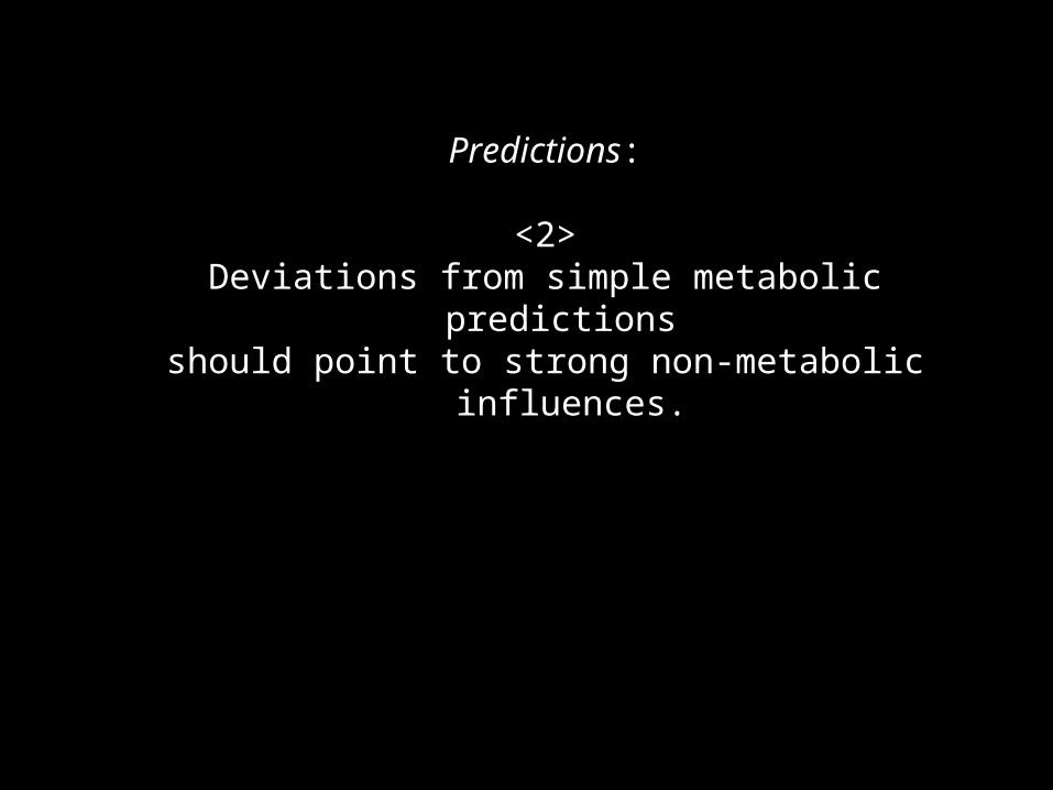
Predictions:

<2>Deviations from simple metabolic predictions

should point to strong non-metabolic influences.

Goal:

De-trend the "metabolic baseline" of complex systems to gain insight into other important ecological processes.

SuccessfullyPredict

FailPredictably

Berlow 1999 Nature 398:330

R

T

Whelks

MusselsBarnacles

Space

R

T

Whelks

MusselsBarnacles

Space

Field Experiment Conditions

R

T

Whelks

MusselsBarnacles

Space

R

T

Whelks

MusselsBarnacles

Space

+-

+- -

- -

Metabolic

R

T

Whelks

MusselsBarnacles

Space

+-

+- -

- -

Metabolic+

Non-Metabolic

R

T

WhelksMussels

Barnacles

+-

Metabolic+

Non-Metabolic

R

T

R

T+-

+- -

T+-

+- -

R

T

R

T

-

T

-Metabolic

Experimental Design

WhelksExcluded

Low WhelkBiomass

High WhelkBiomass

Natural Variationin Mussels

and Barnacles

4 blocks x 3 start datesx 1-3 yrs

-18

-15

-12

-9

-6

-3

0

log

(abs

TE

)

-15 -12 -9 -6 -3 0log (TS biom)

-6

-3

0

3

6R

esid

uals

log

(abs

PC

)

-15 -12 -9 -6 -3 0log (TS biom)

Lo

g (

|per

ca

pit

a I|

)

Log (T biomass)

Lo

g (

|po

pu

lati

on

I|)

Simulation ResultsLow R BiomassHigh R Biomass

Log (Mussel Biomass)

-1 0 1 2 3

Lo

g (|p

op

ulatio

n

I|)

-3

-2

-1

0

1

-1 0 1 2 3

Lo

g (

| per

cap

ita

I|)

-4

-3

-2

-1

0

Log (Mussel biomass)

Low Whelk BiomassHigh Whelk Biomass

Central TendencyPredicted by Simulations

predicted

Lo

g (

|per

ca

pit

a I|

)L

og

(|p

op

ula

tio

n I

|)

-1 0 1 2 3

Lo

g (

| per

cap

ita

I|)

-4

-3

-2

-1

0

Log (Mussel Biomass)

-1 0 1 2 3

Lo

g (

|po

pu

lati

on

I|)

-3

-2

-1

0

1

R

T

-Metabolic predicted

Log (Mussel biomass)

Lo

g (

|per

ca

pit

a I|

)L

og

(|p

op

ula

tio

n I

|)

Low Whelk BiomassHigh Whelk Biomass

-1 0 1 2 3

Lo

g (

| per

cap

ita

I|)

-4

-3

-2

-1

0

-1 0 1 2 3

Log (Mussel Biomass)

-1 0 1 2 3

Lo

g (

|po

pu

lati

on

I|)

-3

-2

-1

0

1

Log (Mussel Biomass)

-1 0 1 2 3

R

T

R

T+

+- --

R2 = 0.49

R2 = 0.43

Metabolic predicted

observed

Log (Mussel biomass)

Lo

g (

|per

ca

pit

a I|

)L

og

(|p

op

ula

tio

n I

|)

Low Whelk BiomassHigh Whelk Biomass

Low Whelk BiomassHigh Whelk Biomass

-1 0 1 2 3

Lo

g (

| per

cap

ita

I|)

-4

-3

-2

-1

0

-1 0 1 2 3

Log (Mussel Biomass)

-1 0 1 2 3

Lo

g (

|po

pu

lati

on

I|)

-3

-2

-1

0

1

Log (Mussel Biomass)

-1 0 1 2 3

R

T

R

T+

+- --

R2 = 0.49

R2 = 0.43

Metabolic Metabolic+

Non-Metabolic

Log (Mussel biomass) Log (Mussel biomass)

predicted

observed

Lo

g (

|per

ca

pit

a I|

)L

og

(|p

op

ula

tio

n I

|)

Summary<1>

¾ power law signal disappears andnew simple patterns emerge in a network context.

<2>magnitude of per capita and population I

explained by 2-3 simple species attributes (of 90)

<3>effects dampen with distancemore complex = more simple

<4>predictable fit and lack-of-fit in field experiment

Conclusions

<1>metabolic "webbiness" of life not necessarily a big source of uncertainty.

Conclusions

<2>“module” approaches may work best

when embedded in complexity

Conclusions

<3>metabolic "null model" may describe

a universal baseline of species interactions in a complex network.

Conclusions

<4>"de-trend" metabolism in ecological networks

to better understand non-metabolic interactions and processes

"I would not give a fig for simplicity on this side of complexity, but I'd give my life for the simplicity on the other side of complexity"

Oliver Wendell Holmes, Jr.

Acknowledgements

Alexander von Humboldt Foundation

-14

-12

-10

-8

-6

-4

-2

0

2

4L

og

(P

op

ula

tio

n D

ensi

ty)

-6 -4 -2 0 2 4 6 8 10 12

Log (Body Mass)

R2 = 0.96 slope = -1.05High Biomass

R2 = 0.36 slope = -1.17Low Biomass

R2 = 0.59slope = -1.4All Points

0.05

0.10

0.15

Pro

babi

lity

-16 -14 -12 -10 -8 -6 -4 -2 0 1

0.05

0.10

0.15

-16 -14 -12 -10 -8 -6 -4 -2 0 1

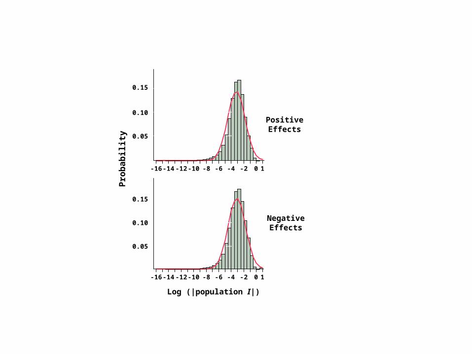
PositiveEffects

NegativeEffects

Pro

bab

ility

0.10

0.05

0.15

0.10

0.05

0.15

Log (|population I|)

n = 5 random subsamplesof 10,000 interactions

trophic

leve

l

1dgr p

rey

biom

log (b

ody m

ass)

#1 d

gr pre

d

% o

f E

xpla

ined

Var

iati

on

0

10

20

30

40

50

R presentR removed

(a)+

+

-

-

Degrees Separated1 2 3 4 5 6 7

Ma

x L

og

(|p

er c

apit

a I|

)

2

4

6

8

10

Ma

x L

og

(|p

op

ula

tio

n I

|)

-1.6

-1.2

-0.8

-0.4

Chains of interactions tend to dampen with distance