Susan Taylor, James H. Lever, Ralph P. Harvey, and May 1997John Govoni

CR

REL

REP

OR

T 9

7-1

Collecting Micrometeorites from theSouth Pole Water Well

Abstract: A collector was designed and built to retrievemicrometeorites from the floor of the South Pole WaterWell. The large volume of firn and ice being melted forthe well and the low component of terrestrial materialin Antarctic ice make the South Pole Water Well anideal place to collect micrometeorites. Because the ageof the ice being melted is known, yearly or periodic

How to get copies of CRREL technical publications:

Department of Defense personnel and contractors may order reports through the Defense Technical Information Center:DTIC-BR SUITE 09448725 JOHN J KINGMAN RDFT BELVOIR VA 22060-6218Telephone 1 800 225 3842E-mail help@dtic.mil

msorders@dtic.milWWW http://www.dtic.dla.mil/

All others may order reports through the National Technical Information Service:NTIS5285 PORT ROYAL RDSPRINGFIELD VA 22161Telephone 1 703 487 4650

1 703 487 4639 (TDD for the hearing-impaired)E-mail orders@ntis.fedworld.govWWW http://www.fedworld.gov/ntis/ntishome.html

A complete list of all CRREL technical publications is available from:USACRREL (CECRL-LP)72 LYME RDHANOVER NH 03755-1290Telephone 1 603 646 4338E-mail techpubs@crrel.usace.army.mil

For information on all aspects of the Cold Regions Research and Engineering Laboratory, visit our World Wide Web site:http://www.crrel.usace.army.mil

collections provide large numbers of micrometeorites ofknown terrestrial age. The collector was designed to poseno threat to the well’s water quality, to be reliable andeasy to operate, and to collect particles larger than 50µm. This report details how this collector was built andtested and documents the rationale behind some of thedesign choices. It also includes preliminary findings fromthe first deployment.

Susan Taylor, James H. Lever, Ralph P. Harvey, and May 1997John Govoni

CRREL Report 97-1

Collecting Micrometeorites from theSouth Pole Water Well

Prepared for

OFFICE OF THE CHIEF OF ENGINEERS

Approved for public release; distribution is unlimited.

US Army Corpsof Engineers®

Cold Regions Research &Engineering Laboratory

PREFACE

This report was prepared by Susan Taylor, Research Physical Scientist, Geologi-cal Science Division; James Lever, Mechanical Engineer, Ice Engineering ResearchDivision; and John Govoni, Physical Science Technician, Snow and Ice Division; ofthe Research and Engineering Directorate of the U.S. Army Corps of EngineersCold Regions Research and Engineering Laboratory; and Ralph Harvey, Senior Re-search Associate, Department of Geological Sciences, Case Western Reserve Uni-versity, Cleveland, Ohio.

Funding for this work was provided by the National Science Foundation. Thereport was technically reviewed by John Rand and Stephen Ackley of CRREL.

The authors wish to thank the following people who assisted in this study: Rob-ert Forrest, William Birch, and Peter Alekseiunas, who made the components forthe micrometeorite collector at CRREL; Michael Walsh, who suggested the tech-nique for fabricating the collector arm; Dennis Lambert, who turned our ideas intodetailed drawings and added improvements of his own; John Rand, who providedinvaluable information about the well and the wellhouse; the CRREL brainstorm-ing participants—Dr. Thomas Jenkins, Janet Hardy, Dr. Edgar Andreas, DeborahDiemand, Stephen Flanders, Capt. Jeffrey Wilkinson, John Rand, and Dr. J.-C.Tatinclaux—for their wonderful and varied suggestions for the collector design;Dr. Ellen Mosley Thompson, The Ohio State University, who kindly provided un-published data on particle size distributions obtained from a South Pole core; PeterStark, who constructed the wooden well shape on which the collectors were tested;Thomas Vaughan for his illustrations; and Jesse Stanley, who juggled his basin testsso that these tests could be run at all hours of day and night. The authors also thankMs. Hodgdon’s 8th-grade math class at Lebanon Junior High School, Lebanon, N.H.,who designed the logo for the project, shown on the cover of this report. Last butnot least, the authors thank Michael Shandrick, who assisted them at the Pole dur-ing the marathon drilling session and any other time his help was needed, for hisdedication and good spirit.

The contents of this report are not to be used for advertising or promotionalpurposes. Citation of brand names does not constitute an official endorsement orapproval of the use of such commercial products.

ii

iii

CONTENTSPage

Preface ..................................................................................................................... iiIntroduction ............................................................................................................ 1South Pole Water Well ........................................................................................... 2Collector design ..................................................................................................... 4

Technical objectives ....................................................................................... 4Design requirements and performance criteria ........................................ 4Preliminary design ........................................................................................ 5Particulate concentrations expected ........................................................... 6

Pumping requirements and preliminary tests .................................................. 7Final design ............................................................................................................ 8

Prototype tests and modifications ............................................................... 10Deployment .................................................................................................... 13

Samples ................................................................................................................... 15Weathering ...................................................................................................... 18Flux rates ......................................................................................................... 18

Conclusion .............................................................................................................. 21Literature cited ....................................................................................................... 22Appendix A: SPWW dimensions ........................................................................ 25Appendix B: Summary of collector development tests .................................... 35Appendix C: Summary of collector deployments in SPWW .......................... 37Abstract ................................................................................................................... 39

ILLUSTRATIONS

Figure1. Evolution of the South Pole Water Well .................................................. 32. Approximate size and shape of the South Pole Water Well

in December 1995 .................................................................................. 43. Original collector concept .......................................................................... 54. Number and size distribution of particles >50 µm estimated

for the bottom of the SPWW ............................................................... 65. Final collector-arm cross-section .............................................................. 86. Major components of the 1.2-m operational collector .............................. 97. Schematic of the 1.2-m collector in the SPWW ....................................... 108. 2.5-m operational collector suspended from the cable on a winch ..... 119. Slot width measured along the 1.2-m collector prior to

deployment ............................................................................................ 1310. Work space at the SPWW, consisting of a winch room directly

over the access hole and an adjoining laboratory ............................ 1411. Hot-water drill used to drill second access hole to the SPWW ............ 1412. Map of the bottom of the SPWW showing the plateau area

and pocket no. 1 .................................................................................... 1513. An assortment of spherules from the SPWW ......................................... 1614. Sediment retrieved from the well ............................................................. 1715. Backscattered electron photomicrographs of selected SPWW

micrometeorites ..................................................................................... 1916. Ternary diagram illustrating where the analyzed SPWW

spherules plot in relation to the Deep Sea and Greenlandspherules ................................................................................................ 20

17. Weight percent Al/Si and Ca/Al plot of the SPWW spherulesas compared to DSS and chondritic value ........................................ 20

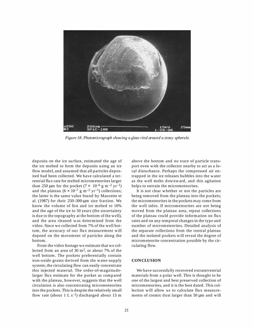
18. Photomicrograph showing a glass rind around a stonyspherule .................................................................................................. 21

TABLESPage

Table1. Other wells built in polar regions ............................................................. 22. Summary of quantitative collection efficiency tests .............................. 113. Size range and weight of the pocket and plateau samples ................... 174. Types of extraterrestrial particles in the pocket sample ........................ 185. Comparison of SPWW spherule types with those found in

Greenland and in the Deep Sea collection......................................... 20

iv

INTRODUCTION

Micrometeorites are the dominant mass contri-bution to the present-day Earth and add one hun-dred tons of material to the Earth each day(Brownlee 1981, Love and Brownlee 1993). Al-though ubiquitous in terrestrial environments,relatively little of this material has been collectedbecause micrometeorites occur in low concentra-tions and generally weather rapidly. To collect mi-crometeorites one needs to find deposits wherethey are concentrated. Like meteorites, micro-meteorites range from unaltered primordial ma-terials to those that have seen extensive differen-tiation and alteration deep within a parent body.They represent collision-produced fragments ofasteroids as well as materials of cometary origin(Brownlee et al. 1993). Some of these small par-ticles are thought to contain exotic materials, in-cluding interstellar grains and fragments of solarsystem materials that have no counterparts amongmeteorite collections (Bradley et al. 1989, Brownleeet al. 1993).

In this paper we use the word micrometeoriteas a generic term referring to all types of terrestri-ally collected extraterrestrial debris with sizes <1cm. Cosmic spherules refer to spherical and/orrounded particles that have been totally or par-tially melted by atmospheric entry. The term in-terplanetary dust particle (IDP) refers to the small(<50 µm) extraterrestrial particles collected in thestratosphere.

More than a century ago a few magnetic cos-mic spherules were found in deep-sea sedimentscollected by members of the H.M.S. Challenger ex-pedition (Murray and Renard 1876). Both iron andsilicate spherules were found, and it was thought,especially of the iron spherules, which containednickel in chondritic proportions, that they were ofmeteoritic origin. The presence of wustite in thesespherules, a high-temperature iron oxide found inmeteorite fusion crusts, also suggested an extra-terrestrial origin for iron spherules (Marvin andEinaudi 1967). The extraterrestrial origin of thesilicate spherules, which are composed of olivine,interstitial glass, and magnetite, was more diffi-cult to prove. Major element analysis showed that

they had chondritic ratios of magnesium, silicon,and iron (Blanchard et al. 1978), but it requiredtrace chemical analyses to show their extraterres-trial origin (Ganapathy et al. 1978).

Cosmic spherules are distinctive-looking par-ticles and have been found in many terrestrial en-vironments. They have been found in the swampsof Siberia (Krinov 1959), in desert sands(Fredriksson and Gowdy 1963), in beach sand(Marvin and Einaudi 1967), in deep sea sediments(Brownlee 1979), in lithified abyssal sedimentsexposed on land (Czajkowski et al. 1983, Jehannoet al. 1988, Taylor and Brownlee 1991), in Green-land’s cryoconite and melt-water drainage basins(Maurette et al. 1986, 1987; Robin et al. 1990), andin Antarctic morainal sediments (Hagen 1988,Koeberl and Hagen 1989), aeolian debris (Harveyand Maurette 1991, Hagen et al. 1992), and ice cores(Yiou and Raisbeck 1990, Hagen et al. 1992).

Unmelted micrometeorites have also beensought and found. Interplanetary dust particles(IDPs) were collected in the stratosphere(Brownlee et al. 1977) and are routinely collectedby NASA using U-2 high-flying aircraft. Largerunmelted micrometeorites were found inGreenland ice (Maurette et al. 1987), and manymicrometeorites, primarily <100 µm in size, werefound upon melting and sieving 100 tons of Ant-arctic blue ice (Maurette et al. 1991).

The South Pole Water Well (SPWW) is a 24-m-diameter by 15-m-deep melt pool 100 m below thesnow surface; it supplies potable water to theAmundsen–Scott South Pole Station. Because ofthe large volume of ice melted, the well is the larg-est source of micrometeorites yet discovered. Thecompressed-snow polar ice preserves a record ofmelted and unmelted micrometeorites in an envi-ronment low in terrestrial debris, and the well pro-vides the concentrating mechanism necessary forcollecting these particles. The large pool volumeand low water-injection rate produce low circula-tion velocities that cannot entrain micrometeoritesmelted out of the ice. These particles should, there-fore, form a lag deposit on the well bottom. Basedon this assumption, we built a collector to retrievemicrometeorites larger than 50 µm from the bot-tom of the well. We deployed the collector in De-

Collecting Micrometeorites from the South Pole Water WellSUSAN TAYLOR, JAMES H. LEVER, RALPH P. HARVEY, AND JOHN GOVONI

1

cember 1995 and did indeed recover large num-bers of micrometeorites.

The SPWW represents a uniquely valuablesource of micrometeorites. The age of the ice be-ing melted is known as a function of depth(Kuivinen et al. 1982), making it possible to datethe depositional age of the particles recovered.Although the SPWW does not allow horizontal(stratigraphic) control on a fine scale as do tradi-tional cores, the large numbers of extraterrestrialparticles from different time periods should allowa statistically significant study of the recent varia-tion of cosmic dust flux at the Earth’s surface. Thefirst year’s collection is an integrated sample ofmicrometeorites that fell to Earth between 1100and 1500 A.D. As melting occurs predominantlyin a downward (older ice) direction at a known

rate, later collections will be integrated samplesfrom known depths, and thus known ages. Morespecifically, the well deepens approximately 10 meach year (equivalent to 100 years of deposition)and will melt ice that dates from 400 to 1500 A.D.during its life. By sampling all, or a known per-centage, of the well bottom and repeating the col-lection on an annual basis, the flux rate and anyvariation in either rate or composition of micromete-orites can be determined on a 100-year time scale.

SOUTH POLE WATER WELL

In 1955 Henri Bader suggested building ‘waterwells’ at glacier camps after observing the size andshape of sewage disposal pits (Clark 1965). Schmitt

Table 1. Other wells built in polar regions.

Date Type Location Additional information

1959 Water wella Camp Century, Greenland Rodriguez assembles components and firstwell is made. Well reached 171.5 ft. Observerlowered into the well after most of the waterhad been pumped out (Schmitt and Rodriguez1960).

1960 Water wella Camp Century, Greenland Original well is restarted, producing a 244-ftsymmetrical, bell-shaped cavity (Schmitt andRodriguez 1963).

1960–1963 Waste heat Camp Century, Greenland Made from waste heat from a nuclear reactorstorageb (Clark 1965).

1960–1961 Water well Tuto, Greenland Russell (1965).

1964 Water wellc Camp Century, Greenland Second utility well created.

1972 Water well South Pole, Antarctica Operated 3 months (Williams 1974).

1977–78 Drilling water Ross Ice Shelf, Antarctica

1990–91 Water welld South Pole, Antarctica Drilled by John Rand and John Govoni. Minedfor micrometeorites in December 1995.

1994–95 Drilling water South Pole, Antarctica Amanda Project, PICO

2

and Rodriguez (1960) were the first to build a melt-pocket water well in ice, and subsequent polarwells have been called Rodriguez or Rod wells (seeTable 1 for a list of such wells). Researchers havesearched for cosmic spherules and extraterrestrialmaterials in polar wells (e.g., Langway 1963,McCorkell et al. 1970). McCorkell and his col-leagues filtered 200,000 liters of water pumpedfrom a meter from the well floor at the Camp Cen-tury well in Greenland. They found no excess 26Al,an extraterrestrial marker, on their 3-µm filters. Themicrometeorites had probably formed a lag de-posit on the well floor, but the pump intake wastoo high on the well bottom to entrain the particles.

The SPWW is a Rodriguez well constructedduring the 1992–93 austral summer. A hot-waterdrill was used to melt a 30-cm-diameter hole intothe snow to a depth of 60–70 m. The drill was thenlowered more slowly to create a large pool or res-ervoir of water. The surface wellhouse, which con-tains the equipment for drilling and operating thewell, consists of two stacked 4.6 × 2.1 × 2.4 m ship-ping containers (millvans). The wellhead is in thelower container, about 2.5 m below the presentsnow surface. The 30-cm-diam. wellhead and neckaccommodate the electrical cable connected to thesubmersible pump, emergency heat trace, and two

insulated hoses (one carrying water to the surfaceand one returning warm water to the well). Be-cause contamination of the well by fuel was amajor concern, a low-temperature EPDM (ethyl-ene propylene dienemonomer) mat surrounds thewellhead and extends out 7 m.

The SPWW was certified as a source of potablewater in early 1994. On 26 February 1994, the poolwas about 16 m deep and 22 m in diameter, andthe well bottom was 101 m below the wellhouse(103.5 m below the snow surface, Appendix A).Before consumption began, however, an electricalfire in the pump cable on 1 March 1994 forced a 9-month shutdown. During the shutdown, a 4-m-thick ice layer formed on the pool surface and 6–11 m of freezeback occurred on the walls and bot-tom. The well was restarted in December 1994 bydrilling through the ice layer and recirculatingwarm water as before. By March 1995, the wellhad melted below the prefire level and releasedany particles trapped during the freezeback. Fig-ure 1 shows the approximate well geometry be-fore and after the fire and at the time of deploy-ment in December 1995. It also shows the corre-sponding age of the ice (and the depositional ageof the micrometeorites).

The SPWW has supplied potable water since

Start Consumption30 Jan 95

Volume Consumed1,600 m3 to end

Dec 95

101.2 m1000 A.D.

86.6 m

90.2 m

D ~ 22 m

26 Feb 94Before Fire on

1 Mar 94Freezeback Before

Restart on 30 Nov 94

106.5 m

Pump

Pool Volume ~ 4,000 m3

1500 A.D.

4 m Ice She

10 cm Ice Cover

60

70

80

90

100

110

Dep

th (

m)

Pool Volume ~5,000 m3

82.6 m

Figure 1. Evolution of the South Pole Water Well.

3

January 1995. The reservoir has reached a rela-tively stable size of about 24 m diameter and 16 mdepth and contains about 5,000 m3 of water (basedon water consumption and depth data, AppendixA). The present consumption rate is about 2,000m3 (about 2 million liters) per year. The pumpdraws water from about 1 m below the water sur-face. About 10% of the water is consumed and therest is heated, using waste heat from the station,and returned to the well.

The flow rate of returning water is about 1L s–1, and it is discharged 3 m below the watersurface through a nozzle designed to produce auniform, 90° cone-shaped jet. Peak discharge ve-locity 1 m away from the nozzle should be lessthan 1 mm s–1, and no remnants of the jetshould persist at the well bottom. Rather, thejet and heat input probably establish large-scalecirculation cells in the pool. It seems very unlikelythat circulation velocities at the well bottom wouldbe adequate to entrain the micrometeorites ofinterest.

The effort required to model the flow distribu-tion in the SPWW was beyond the scope of ourwork. However, we estimated the velocitiesneeded to transport micrometeorites and assessedwhether such velocities were likely to be present.To initiate movement of a 50-µm particle with adensity of 2.5 g cm–3 (stony or glassy micromete-orites), flow velocity along the well bottom wouldneed to exceed about 6 cm s–1 (ASCE 1975). Themicrometeorites of interest are generally larger ormore dense and hence would have higher thresh-olds. It seems unlikely that bottom velocitieswould exceed threshold values, given that veloci-ties 1 m from the nozzle are substantially lower.We therefore thought that micrometeorites wouldform a lag deposit on the well bottom as they aremelted out of the ice.

Originally we had planned to deploy the col-lector during an annual maintenance period whenthe well’s pump and hoses were removed for ser-vicing.* However, space in the well house is verylimited, complicating collector deployment, andour collection time would have been restricted toa few hours. For these reasons we drilled a sec-ond access hole, about 2 m from the centralhole, and had a separate work area constructed(Fig. 2).

COLLECTOR DESIGN

Technical objectivesOur technical objectives were (a) to collect es-

sentially all of the micrometeorites from a large,known area of the well bottom, and (b) to be ca-pable of returning to the same area of the wellbottom annually. Assuming that the micromete-orites form a lag deposit, meeting these technicalobjectives would allow us to calculate flux ratesand document any temporal changes in the com-position of the particles (i.e., meet the scientificobjectives).

Design requirements and performance criteriaThe nature of the SPWW imposes strict require-

ments on the collector design. The collector mustnot degrade water quality under any circum-stances. It must fit down a 30-cm-diam. well neckand survive a cold soak at –50°C during its de-scent to the well pool. It must operate remotely inabout 20 m of water at a distance of 200 m belowthe snow surface.

In addition, we specified several performancecriteria to help guide our design selections. Thecollector should collect essentially all particles in

Surface

Winch Room

WellhouseLab

2.5 m

60 m

70 m

80 m

90 m

100 m

110 m 24 m

EPDM Protective

Mat

1500 A.D.

1000 A.D.

Cameraand Lamp

Water Level

Collector

Figure 2. Approximate size and shape of the South PoleWater Well in December 1995.

*J.H. Rand, 1996, Ice Engineering Division, CRREL, per-sonal communication.

4

the size range 50–1000 µm without bias to compo-sition (e.g., toward magnetic particles). Its collec-tion efficiency should be high (and we shouldmeasure it). It should cause no physical or chemi-cal changes to the particles. Its design should mini-mize handling losses after collection. It should givereliable performance and be adaptable to un-known bottom surface conditions. In addition, itsdesign should minimize the possibility of it be-coming stuck in the well.

Preliminary designWe had a brainstorming session to gather pre-

liminary collector concepts. After reviewing theseideas, we selected a concept that involved down-hole suctioning and filtering of the particles by amobile collector controlled from the surface. Fig-ure 3 shows this concept as originally envisioned.It utilizes the unconstrained, vertical dimensionof the well neck to maximize the filter capacity andthe area swept out by the collector in a single pass.A pump develops a high-speed flow to suctionparticles through a slot along the underside of along, flexible arm containing a filter. The filter armwould be formed from a flexible, drinking-water-safe plastic to allow it to conform to the curvedwell bottom. We could drive the long arm aroundin a circle and measure its rotation to determine

the area swept. Separate filter chambers distrib-uted along the arm would reveal informationabout the radial distribution of particles. Alterna-tively, we could independently operate a drivemotor at either end of a shorter version of the col-lector to maneuver it over undulating well-bot-tom topography. An underwater video camerawould help maneuver the collector and documentthe area swept.

This concept contains many advantages overalternatives considered. Suctioning particles by en-training them in a water stream should avoid anycompositional bias in the collection (assuming thatthe water flow is high enough to entrain the heavi-est particles of interest). Down-hole filteringavoids the need to pump water and particles tothe surface, saving pumping requirements andavoiding particle damage and losses within thepiping system. Indeed, our design minimizes par-ticle damage and losses by incorporating the fil-ter immediately downstream of the intake slot.

Further development of this concept requiredbasic data on the number of particles expected (todetermine filter capacity), the flow velocity neededto entrain the particles of interest, and the pump-ing losses expected (to size the pump). We alsoinvestigated several fabrication options to incor-porate a filter into the collector arm.

Figure 3. Original collector concept (layout and filter arm cross-section).

5

Particulate concentrations expectedWe determined the filter mesh size and required

area using information on the size distribution andamounts of particulates in Antarctic ice and esti-mates of extraterrestrial particle concentrations inGreenland and Antarctic ice.

The number of particulates in Antarctic ice <30µm have been determined using Coulter counters(unpublished data from E.M. Thompson) and bycounting the number of particles from photomi-crographs taken using a scanning electron micro-scope (Higashi et al. 1990). The number of particlesis very high: 20,000 particles/mL of water for sizesless than 1 µm, and about 7000 particles/mL ofwater in the 1–30-µm size range (unpublished datafrom E.M. Thompson). These particles are over-whelmingly terrestrial in origin. Thus, to avoidclogging our filter with terrestrial particles, wechose a filter fabric with a 53-µm opening. Thisshould limit our collection to particles larger thanabout 50 µm unless the filter plugs significantly.These larger particles are easy to handle and ana-lyze.

We estimated the fraction of extraterrestrial toterrestrial particles in Antarctic ice larger than 50µm using data from Maurette et al. (1991). Theymelted 100 tons of Antarctic ice and recoveredabout 10 grams of particulate material. This mate-rial included 9000 micrometeorites 50 to 100 µmin diameter, 6500 micrometeorites 100 to 400 µmin diameter, and 9 micrometeorites larger than 400µm. Assuming an average density of 2.5 g cm–3,and taking 75 µm as the average diameter for the50- to 100-µm-sized particles, 250 µm for the 100-to 400-µm particles, and 400 µm as the diameter

for particles larger than 400 µm, we estimate that0.15 g of the 10 g recovered, or about 1.5%, wasextraterrestrial.

Maurette et al. (1987) estimated the microme-teorite flux rate falling on Greenland ice as 6.3 ×10–6 g m–2 yr–1 for the 50–300-µm size range. Loveand Brownlee (1993) measured the micrometeor-ite flux rate in space, using the Long Duration Ef-fects Facility, as 40 (±20) × 106 kg yr–1, or 1.2 ×10–4 to 3.9 × 10–5 g m–2 yr–1. The difference be-tween the LDEF and the Greenland values sug-gests that 5 to 15% of the particles survive atmo-spheric passage. Figure 4 shows the size distribu-tion of micrometeorites expected at the SPWWbased on the Greenland flux rate. Our original es-timate for the diameter of the SPWW was 15 mand that 10 m of downward melting (100 years ofdeposition) would occur each year. Thus, we ex-pected that yearly collection could yield 0.11 gramsof micrometeorites, or about 105 particles largerthan 50 µm based on the flux rate of Maurette etal. (1987). However, we expected the first collec-tion in 1995–96 to have three to four times thisamount of material because of the larger ice vol-ume melted to create and operate the well prior toour deployment.

We also expected the operation of the SPWWto add particulates to the well. To determine anapproximate count, we asked John Rand to filter8 L of water from the SPWW through a cellulosenitrate membrane filter with a 5-µm pore size. Weexamined the filter both optically and with a scan-ning electron microscope. Eleven percent of thesurface area of the filter yielded 15 fibers and 568particles, most in the 5–10-µm size range. Forty-

5

3

2

1

0

4105

104

103

102

106

50 100 150 200 250 300Mean Particle Diameter (µm)

Num

ber

of P

artic

les

Flu

x R

ate

(10–

6 g

m-2

yr-

1 )

Flux Rate (Maurette et al. 1987)No. of Particles in First YearNo. of Particles Released in 1 Year

Figure 4. Number and size distribution of particles >50 µm estimated forthe bottom of the SPWW.

6

four particles were larger than 50 µm. A randomsampling of these particles using an SEM/EDXfound a copper sulfate grain, an alumino silicatewith some CuS on its surface, a fibrous particle(probably plastic) with some mineral fragmentsadhered, a very platey alumino silicate that con-tained Mg, Ca, and Fe, possibly a clay, several plas-tic pieces, and four particles containing Fe, Ni, Cr,Pb, Al, Si, and a trace of S. Most of these particlesprobably come from the heat exchanger, pump,and hoses used to operate the well. Assuming thatthe number of particles found in the 8-L sample isrepresentative of what would be found in 2000 m3

(the amount of water melted during one year ofoperation), that all these particles were from thewell equipment, and that they settle to the bottomand are collected by our device, 108 terrestrial par-ticles would be added to our collection, or about1000 terrestrial particles for each extraterrestrialparticle larger than 50 µm. Annual collectionwould thus yield a total of about 100 g of material.

The 8-L sample also revealed the presence ofsubmicron particles of iron oxide in the well wa-ter. The white, cellulose nitrate membrane filterturned a bright orangish color after filtration, andenergy-dispersive X-ray analyses of the filtershowed only the presence of iron. The rust isthought to be from the heat exchangers or pumpused for the well. Until January 1994, the water inthe SPWW was acidic (pH 4.8), very soft,* and cor-rosive to metals. NSF has neutralized the water(pH 6.9) by running it through a limestone bed.This measure may diminish the formation of ironoxide. In addition, a fire retardant (Ansul dust,similar to baking soda) was used during the 1994well fire. Particles of this fire retardant, soot, andmelted insulation could also have reached the wellpool, although most should have deposited alongthe well neck.

PUMPING REQUIREMENTS ANDPRELIMINARY TESTS

Our collector design allowed for almost 1 m2

of 30-cm-wide filter fabric inside a 3-m-long filterarm using a single fold of the filter to create apouch. We obtained a polyester filter consistingof 53-µm mesh openings and 108 openings/m2.Thus, 1 m2 of this filter should trap the expected

108 particles before plugging. Design guidancesuggested using a pressure drop of 34 kPa (5 lbin.–2) across the filter to determine pumping re-quirements. We expected that this loss woulddominate all pumping losses.

We estimated the required pumping rate fromthe velocity needed to entrain 1-mm-diametersand particles in water (ASCE 1975). The averagevelocity in the intake slot must exceed the particlefall velocity of about 10 cm/s to carry these par-ticles into the filter. In addition, the friction veloc-ity between the filter arm and the ice surface mustexceed the threshold value to initiate particlemovement of about 3 cm s–1. This requires thatthe average flow exceed about 15 cm s–1, if we as-sume that the gap between the filter arm and theice surface is about 1 mm. Both conditions are metif the average velocity exceeds 30 cm s–1 in a 1-mm-wide intake slot (or 15 cm s–1 in a 2-mm-wideintake slot). We selected a compact, submersiblepump that could deliver 1.6 L s–1 at 34 kPa or about50 cm/s through a 1-mm-wide × 3-m-long intakeslot. Near zero pressure, the pump delivers about3 L s–1 (100 cm/s through a 1-mm-wide × 3-m-long intake slot).

We expected that the high-pressure dropthrough the filter and the narrow intake slot wouldestablish relatively uniform intake velocities alongthe slot. Nevertheless, we conducted flow tests ona 30-cm-long × 13-cm-wide model of the filter arm(front-slot version, Fig. 3) to verify particle pickupand assess the velocity distribution. This modelcontained pressure taps that allowed us to mea-sure the pressure drop across the intake, the filter,and the plenum areas at three cross-sections alongthe collector. We also measured the total flow rate.For these tests, we prepared mixtures of simulatedextraterrestrial particles consisting of stainless steeland glass spheres and silica sand, covering a sizerange of 50–420 µm.

We found no appreciable plugging of the filter(negligible increase in pressure drop across filter,negligible decrease in flow rate) even after collect-ing 68 g of material. The maximum pressure dropacross the 53-µm filter was 4.2 kPa, and the corre-sponding minimum flow rate was 0.31 L s–1 (rep-resenting 100 cm s–1 through the 1-mm-wide × 30-cm-long intake slot). The collector model easilysuctioned up particles lying several millimeters infront of the intake. However, because the flowvelocity drops quickly inside the collector, the col-lected particles were deposited on the bottom ofthe filter pouch downstream of the slot rather thanevenly plugging the fabric.

*H. Mahar, 1996, National Science Foundation, personalcommunication.

7

These tests also revealed several disadvantagesof our original, front-slot design: (a) filter installa-tion was awkward, (b) it would be difficult to con-trol the slot width if the arm was made from flex-ible plastic, and (c) the flow-collecting plenumchannel downstream of the filter needed to belarger to reduce the pressure drop (and hencemaintain a more uniform intake velocity distribu-tion) along the collector arm.

For these reasons, we modified the collector-arm design to produce a central intake slot and aflow plenum channel along each side (Fig. 5). Thearm can be fabricated from a machined and foldedpiece of low-density polyethylene (LDPE). O-ringssecure the sides of the filter fabric adjacent to theintake slot, and folding results in a filter pouch.End caps with O-rings seal the filter pouch andprevent flow leakage. Aluminum ribs spacedalong the arm maintain the geometry of the armand slot and prevent collapse of the plastic undersuction. Although this design draws flow equallyfrom both directions under the collector, resultingin lower velocities along the ice surface, we feltthe manufacturing, assembly, and flow-distribu-tion advantages outweighed this disadvantage.

We conducted flow tests on a 30-cm-long × 18-cm-wide model of the central-slot collector arm.This model developed better flow distribution, asevidenced by a lower pressure drop through thefilter and negligible pressure drop along the ple-num channels. It also easily suctioned up the testparticles. No appreciable plugging of the filter oc-curred even though it collected almost 200 g ofmaterial, and the resulting minimum flow rate was0.33 L s–1. It was also much easier to install andremove filters with this model. With careful ma-chining, a relatively uniform intake slot was

formed by folding and securing the two sides ofthe arm.

An important modification resulted from thesetests. We found that particles could escape backthrough the intake slot when we pulled the col-lector out of the water and the pump lost suction.To prevent this “backflushing” of particles, weinstalled a thin strip of 1-µm filter fabric (laterreplaced with a strip of thin LDPE) to serve as aflow check valve. This solved the backflushingproblem.

FINAL DESIGN

We constructed two fully operational collectorsbased on the central-slot design. We initially builta 1.2-m-long prototype to assess the design’smaneuverability and collection efficiency on icedsurfaces. This prototype also provided us with ashorter, more maneuverable collector to use in theSPWW as an alternative to the 3-m-long deviceoriginally planned.

Figure 6 shows the basic features of the 1.2-mcollector. The filter arm consists of a single ma-chined and folded sheet of LDPE with the sameinternal layout as the 30-cm-long model (Fig. 5).This arm is quite flexible, allowing the collector toconform to a surface curvature of about 2 m ra-dius (30 cm rise over 1.2 m). The LDPE also exhib-its low friction on wet ice. A central, waterproofaluminum housing contains the pump and drivemotors and all electrical connections; the externallymounted pump housing is also aluminum. O-ringsseal the removable end plates and motor shafts.Traction is via heavy, stainless steel, spiked wheelsdriven by DC gear motors through articulated alu-

Folded LDPE

Flow Channelto Pump

O–Ring

2 mm Intake Slot

Thin LDPE Strip(check valve to prevent

back–flushing)

Filter Fabric(53 µm mesh)

Aluminum Rib

Figure 5. Final collector-arm cross-section.

8

minum shafts. The manufacturer rated these mo-tors for a continuous duty torque of 4.6 N·m. Ateach end of the arm, heavy aluminum assembliesguide the motor shafts and help the collector con-form to surface curvature. In addition, one of theseend assemblies contains an internal flow passage(manifold) to connect the pump to the two ple-num chambers along the arm.

An electromechanical cable connects to the cen-tral housing via a waterproof connector. This cus-tom-made, LDPE-jacketed cable contains 19 elec-trical conductors to operate the collector, under-water video camera, and lights at the SPWW. Italso contains an internal Kevlar braided jacket,with a rated breaking strength of 4500 N, to act asa strength member. Mechanical attachments at thehousing and end assembly transfer the weight ofthe collector to the cable. This 17-mm-diam. cableis quite flexible and can bend to a minimum ra-dius of 30 cm at –50°C. All collector and cable com-ponents were accepted for use in the SPWW. Fig-ure 7 shows a schematic of the 1.2-m collector,cable, camera, and lights in the SPWW.

We also constructed a 2.4-m-long, central-slotcollector (Fig. 8). We chose this length for the filterarm because the longest sheet of LDPE availableto us was 2.4 m. This collector utilizes similar com-ponents but is completely independent of the 1.2-m collector. It possesses two waterproof housings,each fitted with a pump and drive motor. Both alu-minum end assemblies contain internal manifoldsto connect the pumps to the plenum chambers inthe arm. We can replace one drive wheel and mo-tor with a 90° gear box and rotation transducer tomeasure the rotation of the arm around a pivot

point. The same electromechanical cable operateseither collector. Many of the individual compo-nents are interchangeable between the 1.2-m and2.4-m collectors, providing a level of redundancy;we also purchased numerous spare parts, includ-ing a second electromechanical cable.

The underwater video camera consisted of ahigh-resolution color camera and a zoom lensmounted inside an aluminum pressure housing(rated to 1000-m water depth). A thermostaticallycontrolled heater ensured normal camera opera-tion at –50°C. Two independently operated 500-W waterproof lamps provided illumination, withone projecting sideways from the collector and oneprojecting downward from the camera. Water-proof connectors connected the camera and lampsto the electromechanical cable. This equipmentwas operated through a video control unit and avideo monitor at the surface.

The video system provides the visual feedbackneeded to maneuver the collector. We control therotation speed and direction of drive motors us-ing two DC power supplies at the surface. Cur-rent limiters ensure operation of the motors be-low their continuous-duty torque ratings. A simplerectifier and switch are sufficient to operate thecollector pumps. We can monitor the currentdrawn by the pumps to determine the approxi-mate flow rate.

A reversible, constant-speed winch raises andlowers the collector via the electromechanicalcable. A set of slip rings provide electrical connec-tions between the rotating cable and the station-ary surface equipment. The cable passes over a 76-cm-diam. sheave mounted on top of a 3.6-m high

Figure 6. Major components of the 1.2-m operational collector.

9

tower and then connects to the collector (Fig. 8).The tower allows the collector to hang verticallybefore descending through the well neck; it alsoallows the cable to warm slightly during ascentbefore bending over the sheave. The winch, towerassembly, and video and collector control equip-ment fit inside the winch room located directlyabove the second access hole to the SPWW(Fig. 2).

Prototype tests and modificationsValidating the performance of our particle col-

lection system prior to its first use at the SouthPole was an essential step in our design plan. We

arrived at the final collector designs through a se-ries of laboratory tests, primarily using the 1.2-mcollector prototype. The goals of these tests wereto assess the collector’s maneuverability and col-lection efficiency on submerged, iced surfaces andto make modifications as warranted before build-ing the 2.4-m collector. We used two main test fa-cilities: a 1.5 m × 1.5 m × 0.3-m-deep tank with acold plate on its bottom to grow a flat layer of ice,and a 2.5-m-wide × 6-m-long × 3.6-m-high icedramp with a curved parabolic profile that approxi-mated published shapes for earlier Rodriguezwells (Schmitt and Rodriguez 1963, Russell 1965,Williams 1974, Lunardini and Rand 1995). We

Figure 7. Schematic of the 1.2-m collector in the SPWW.

Center of Well

Camera and Lamp

CollectorOverall Length......120 cm

Maximum Height........23 cmWidth........20 cm

Central Plateau

ParticulateConcentrations

30-60 cm

1-1.5 m 4-5 m

30-60 cm

10

could submerge the iced ramp in a 9-m-wide ×37-m-long × 2.4-m-deep refrigerated basin. Thisprovided the most realistic simulation of the collec-tor’s operation in the SPWW; however, we wereunable to conduct quantitative collection-effi-ciency tests with this arrangement.

We quickly found that collector maneuverabil-ity was very good on both the flat and curved icedsurfaces. The heavy spiked wheels provided ex-cellent traction, and motor torque was adequate

for the collector to climb up the ramp to a locationwith a 45° downward slope. Pump suction did notaffect collector mobility.

We conducted four quantitative collection effi-ciency tests, all using the 1.2-m collector in the 1.5-m iced tank. In all four cases, we used a 53-µmpolyester filter and a 5-cm-wide strip of LDPE asa check valve. We again used mixtures of stainlesssteel, glass spheres, and silica sand to simulatemicrometeorites in a size range 60–400 µm. Weweighed the particulates added to the tank beforetesting and the particulates recovered from thecollector filter after testing to determine the over-all collection efficiency. Table 2 summarizes theresults of these tests.

The ice surface formed on the cold plate wasquite flat across the tank (with only 3- to 5-cm-widestrips of thinner ice along the tank walls) and gen-erally very smooth (with only a few isolated de-pressions 1–2 mm deep and 1–2 cm wide, made aswe added water to fill the tank). We tested the col-lector on this smooth ice during the first, and halfof the second and third, collection-efficiency tests.For half of the second and third tests and all of thefourth test, we roughened the ice with a water jetto create numerous depressions 2–10 mm deep and1–2 cm wide.

The collector suctioned test particles very wellfrom smooth ice surfaces, collecting almost all theparticles in a single pass. Particles remaining afterthe first pass were usually concentrated in the lo-cal depressions. Each additional pass would re-trieve some particles from the depressions, but thecollector would not generally clean them entirely.Nevertheless, the first three tests all yielded col-lection efficiencies over 99% (Table 2) despite thepresence of intentionally roughened ice during halfof the second and third tests. Interestingly, the col-lector achieved these high collection efficienciesdespite leaving clearly visible patches of particles,mostly concentrated in the depressions but also in

Figure 8. 2.5-m operational collector suspended fromthe cable on a winch.

Table 2. Summary of quantitative collection efficiency tests. All tests were con-ducted in 1.5-m iced tank.

Material Materialadded recovered Percent

Date (g) (g) recovered Remarks

29 Jun 390.1 387 99.21 Smooth ice, multiple passes30 Jun 100.1 99.54 99.44 Smooth ice surface 50 g, rough ice 50 g

6 Jul 100.0 99.46 99.46 Smooth ice surface 50 g, rough ice 50 g10 Jul 231.51 206.38 89.15 Rough ice surface

11

lower concentrations on the flat ice. For example,the second test left only 0.6 g of the 100.1 g of par-ticles added, yet particle patches were clearly vis-ible.

The collector had much more difficulty collect-ing particles from the extensively roughened icesurface made for the fourth collection efficiencytest. It achieved a collection efficiency of only about89%. Some of the remaining particles, however,were frozen onto the bottoms of the depressions,suggesting that the test technique may have af-fected the recovery. Nevertheless, we did not knowwhat the SPWW bottom roughness would be like,and we wanted to develop a method to retrieveparticles easily from rough ice.

We made several minor modifications to the col-lector during the collection-efficiency tests basedon the observed performance. The first test re-vealed that the flat-bottomed collector could pressparticles into very flat ice and be unable to collectthem. We subsequently tested the collector with1.5-mm-diam. Teflon-coated wires wrappedaround the filter arm at the locations of the inter-nal ribs. We tested these “runners” during the sec-ond and third tests and found that the collectordid not press the particles into flat ice and itachieved good collection efficiency. However, thecollector could retrieve particles better from deepdepressions without these runners. We stillbrought a quantity of this wire to the SPWW foruse if the well-bottom ice appeared to be verysmooth (we did not use it).

We also developed (but again did not use in theSPWW) a method to retrieve particles from roughice. This involved attaching an 8-cm-wide strip ofthin LDPE (the same material used for the checkvalve) to the underside of the collector arm adja-cent to the slot. This external flap would seal itselfto the ice surface when the pump was on. Flowcould only bypass the flap though deep depres-sions, effectively cleaning these depressions ofparticles, or by entering the slot from the other sideof the collector, essentially doubling flow veloci-ties. We tested this arrangement in a separate col-lection efficiency test on very rough ice. It pickedup particles extremely well, even from 1-cm-deepdepressions, and left the ice visibly clean after asingle pass. Unfortunately, the shipping deadlineprevented us from conducting a quantitativecollection efficiency test, but the visual evidencefrom the test conducted suggests that it wouldhave been greater that 99%.

We routinely measured flow rates through the1.2-m collector during the collection efficiency

tests. The flow rate was consistently 2.1 L s–1,independent of ice conditions, the presence of run-ners, and the amount of material collected (up toa maximum of 212 g preceding a flow measure-ment). Unlike the 30-cm-long model, however, itwas difficult to achieve a uniform slot width alongthe 1.2-m-long prototype. For the first two collec-tion efficiency tests, the slot width averaged about1 mm, but varied between about 0.5 and 1.5 mm.This yielded an average gap velocity of about 170cm s–1, much higher than that needed for particlepickup. Because we were concerned that the nar-row slot sections corresponded to areas of poorparticle pickup, we attempted to machine the slotto a uniform width of 2 mm. We achieved an aver-age slot width of 1.64 mm (Fig. 9), but local varia-tions ranged from just under 1 mm to 2.8 mm. Thisyielded gap velocities that ranged from 64 to 190cm/s and averaged 125 cm s–1 (assuming a uni-formly distributed total flow of 2.1 L s–1), well ex-ceeding the target minimum of 10 cm/s. This ve-locity distribution did not appear to affect overallcollection efficiency (the collector recovered over99% of the particles deployed on combined smoothand rough ice during the third test), and we nolonger saw any correlation between narrow slotwidth and poor particle pickup. We made no fur-ther changes to the slot prior to field deployment.

We also conducted particle-collection tests us-ing the 1.2-m collector in the iced ramp, submergedin the refrigerated basin. Although these tests werequalitative, visual evidence indicated good collec-tion efficiency where the collector contacted thesurface. However, the collector left particle patcheson the ramp in areas where it did not conform wellto the surface shape. We therefore added weightinside the waterproof housing to allow the collec-tor to conform to more severe surface curvature.

The modifications resulting from these tests onthe 1.2-m collector were essentially options to im-prove collection efficiency on very smooth, rough,or curved ice and did not affect the basic design.Thus, we constructed the 2.4-m collector essen-tially as designed (see Appendix B for a summaryof the collector development tests).

We tested the 2.4-m collector only on the iced,submerged ramp. The collector was quite maneu-verable and could sweep across a region with a45° upward slope. However, as with the 1.2-m col-lector, we added extra weight near the center ofthe collector to help it conform to the ramp andthereby improve its collection efficiency (docu-mented visually). The spiked wheels could slip orcut through the ice at the steeper ascent angles, so

12

to increase traction we manufactured longer driveshafts that could accept a double set of heavy,spiked wheels. These same long shafts and thespare wheels also fit the 1.2-m collector (option-ally to increase its traction).

In addition to these tests on the assembled col-lectors, we cold-soaked individual components(silicone hoses, LDPE filter arm, O-rings, etc.) at–65°C in a liquid-nitrogen-cooled chamber(Tantillo 1993) to check their flexibility and dura-bility. We also suspended each collector from ourtower and sheave to ensure that they hung true.

DeploymentWe sent two fully operational collectors to the

South Pole with the means to make modificationsto each should the well-bottom conditions be dif-ferent from our expectations. We also shipped awinch, tower, and sheave, two 200-m electrome-chanical cables, a video camera, monitor, and re-corder, spare pumps, filter fabric, and motors andvarious tools that we needed for assembly andrepair of the collector in Antarctica. The operationof all these components was checked before ship-ping. The collectors and cables were disinfectedusing a 1:60 solution of Clorox® to water and werewrapped in plastic to stay clean during transit.

At the Pole, personnel from Antarctic SupportAssociates (ASA) assisted us in many ways. Theirmain task was to build the surface facilities thatwould provide us access to the SPWW and createan adjoining work space. They first dug a pit(about 3 m × 3 m × 3 m) in the snow adjacent tothe existing wellhouse and down to the EPDMliner. We then cut a 30-cm square opening in the

liner, and ASA constructed and installed an EPDM-lined wooden chimney over the opening. Wesealed the chimney to the opening. This processensured continuity of the EPDM liner around ouraccess hole and work area. ASA then carefullybackfilled the pit with snow and constructed ourwork space. This work space consisted of a winchroom directly over the chimney and an adjoininglaboratory (Fig. 10).

We used a hot-water drill (Fig. 11) to make thesecond access hole to the SPWW; ASA also assistedwith the drilling. Water from the well was heatedin boilers located in the wellhouse and fed intothe 30-cm-diam. cylindrical drill via a neoprenerubber hose. This hot water discharged through a90°-cone nozzle to melt the ice as the drill de-scended. A water pump positioned inside the drillpumped water from down-hole to the surface viaa return hose. The drill was lowered using a winchand stainless steel cable. The hoses were attachedto the cable with stainless clamps and cloth ties.The cable was guided into the hole using a sheavesuspended from a spring scale. The scale allowedus to determine whether the drill was suspendedin air, was on ice, or was in water; this set the drill-ing rate. Drilling took about 36 hours, longer thanexpected, but yielded a vertical, wavy-walled ac-cess hole with a minimum clearance of 30 cm indiameter.

Prior to collector deployment, we lowered thevideo camera to examine the hole and inspectthe well-bottom topography. We noticed that anice cover had formed on the well pool and thatthe access hole through it had refrozen (we wouldneed to break through this ice cover before each

0

3

2

1

0

40

80

120

160

200

0 20 40 60 80 100 120Distance (cm) from Pump End

Slo

t Wid

th (

mm

)

Gap

Vel

ocity

(cm

s-1

)

Slot Width (mm)Average Slot Width (mm)

Average Gap Velocity (cm s-1)Gap Velocity (cm s-1)

Figure 9. Slot width measured along the 1.2-m collector prior todeployment. Also shown is the corresponding gap velocity, assum-ing a uniform distribution of 2.1 L s–1 total flow.

13

collector deployment). More importantly, the cam-era revealed that the well bottom contained iso-lated dark pockets of particulates and thatthese pockets coincided with sculptured featuresin the ice that were arcuate and half a meterdeep. We decided to deploy the 1.2-mcollector because it could more easily negotiatethe sculpted topography than could the 2.4-mcollector.

We successfully deployed and retrieved the 1.2-m collector six times and obtained five separatecollections (one filter deployed twice) totalingabout 200 g of material. Appendix C lists the de-ployments and shows the collector configurationfor each. The collector provided a scale uponwhich to judge the well-bottom topography. It wasmuch more complicated than we expected basedon published shapes of earlier Rodriguez wells(Schmitt and Rodriguez 1963, Russell 1965, Will-iams 1974, Lunardini and Rand 1995). It consistedof a gently curved central plateau (about 18 m2)sculptured at its periphery into fairly steep arcu-ate dips that were 0.3–0.6 m below the plateau and1–3 m wide; these dips led to smaller plateaus (1–3 m2) (Fig. 12). Farther away from the center, thebottom rose steeply and the sculptured featuresappeared to be more severe (either deeper or at

Figure 10. Work space at the SPWW, consisting of a winch room directly over the access hole and anadjoining laboratory.

Figure 11. Hot-water drill used to drill second accesshole to the SPWW.

14

shorter length scales). Associated with most sculp-tured features were dark pockets of particulates.Particles on the plateau areas were visible but notconcentrated into pockets. Local surface roughnesswas quite smooth (perhaps 1-mm depressions over1–5 mm scales). For this reason, we did not usethe Teflon-wire runners or external LDPE flap(developed for very smooth or rough ice, respec-tively).

The collector maneuvered easily over the cen-tral plateau, and we devoted one collection (no. 3)exclusively to the plateau. Movement onto the ad-joining dips and plateaus was possible with somepractice, and we collected from five of these (about10 m2 total), including three particle pockets. Wecollected as much as 50 g of material at oncewithout appreciably reducing pumping efficiency.Plateau areas suctioned were visibly clean, andgently curved dark areas changed from black towhite with a single pass. This indicated high-effi-ciency particle pickup, based on our laboratory ex-perience.

Good contact between the collector bottom andthe ice surface was the most serious limit to col-lection efficiency in severely curved areas, and wemaneuvered the collector slowly across the asso-ciated pockets to maintain good surface contact.This technique worked well but was very time-consuming. During some deployments, the field

of view of the video camera limited our ability tomaneuver the collector. We tried several tech-niques, unsuccessfully, to orient the camera to fol-low the collector.

The spiked wheels, often doubled on each end,provided extremely good traction on the ice. Theallowable motor torque, rather than traction,generally limited collector maneuverability onsteep sections, although collector stability was alsoa factor. We normally worked around these limi-tations quite successfully, and could have substan-tially increased the area suctioned within the per-formance capabilities of the 1.2-m collector. Un-fortunately, after about two hours of maneuver-ing during a deployment, the drive motors failed.Post-deployment inspection revealed that shear-ing of gear teeth in each motor’s gearbox causedthe failures. This repeatedly occurred, despitereadouts from the drive-motor power supplies thatindicated operation at about half of the continu-ous-duty torque rating provided by the motormanufacturer. After all four motors had failed once(by deployment no. 4), we continued to run thecollector by interchanging gears between gear-boxes; this provided us with about two hours ofoperation before motor failure for deployments 5and 6.

We had planned to dedicate deployment no. 4to repeat suctioning of the central plateau. Thiswould have allowed us to calculate in-situ collec-tion efficiency. Unfortunately, one drive motorfailed at the start of that deployment, and we onlycovered about one third of the central plateau.Upon retrieval of the collector, we found very littlematerial in the filter bag and decided to reuse itfor the next deployment to save time. Althoughnot quantitative, the results of deployment no. 4and the visually apparent cleaning of particlesfrom the ice suggests a high in-situ collection effi-ciency.

SAMPLES

After each deployment except no. 4, we broughtthe collector to the laboratory space and removedthe polyester filter from the filter arm. The whiteflexible fabric allowed us to see particles and eas-ily remove them by backflushing the filter. Webackflushed each of the two samples we processedinto a large HDPE funnel, using well water thatwe pressurized in an HDPE hand sprayer. Eachsample, one from a pocket, the other from the pla-teau, was then wet-sieved into stainless steel sieves

Plateau

Pocket 1

Pocket 5 and 6

Collector

Figure 12. Map of the bottom of the SPWW showingthe plateau area and pocket no. 1.

15

yielding 50–106-µm, 106–250-µm, 250–425-µm,and >425-µm size fractions. Using a binocularmicroscope, spheres were separated from thesetwo samples by hand picking (Fig. 13). These twosamples were processed in the field to assess thecollector’s performance and to determine the typeand amount of materials recovered. The remain-ing three samples were placed in bags, sealed, andshipped to CRREL for later analysis.

Other than well water, no solvents were usedin the separation process. We collected aliquots ofeverything the particles may have come in con-tact with (drilling water, water, and residue leftafter backflushing and sieving a collection). Wealso exposed a section of clean filter to thewellhouse environment, as suggested by MichaelZolensky. These samples can be analyzed if anyunexpected contaminants are found in the par-ticles.

About 200 g of material were recovered fromthe well bottom. Most of the material was terres-trial (Fig. 14), predominantly rust grains injectedinto the well and originating either from the heatexchanger or from the non-stainless steel compo-nents within the pump. There were also woodfragments, paint chips, wire, and aluminum flakes.

Our initial examination of the collected sedi-

ment focused predominantly on spherical par-ticles. Although not all spherical particles are extra-terrestrial (there were copper spheres formedwhen pipes were soldered and dark, nonmagnetic“glue balls” thought to have formed during thefire), spheres can be rapidly separated with an or-dinary binocular microscope. Those that are “cos-mic” can then be separated by their several uniqueproperties. Previous studies have shown that cos-mic spherules have distinctive mineralogy, bulkchemistry, internal and surface textures, and areusually moderately magnetic (Brownlee 1981).Here we used their abundance as a measure of theamount of extraterrestrial material in our samples.

All 6.01 g of the 250–425-µm size fraction ofpocket collection no. 1 and all 3.5 g of the 250–425-µm size fraction of the plateau collection wereexamined. Table 3 lists the number of cosmicspherules found in these two fractions. Assumingan average particle weight of 3.5 × 10–5 g/particle(300 µm diam., 2.5 g cm–3) gives a weight of 7.9 ×10–3 g for the pocket collection and 4.4 × 10–3 g forthe plateau collection, or about one part per thou-sand melted meteoritic material. In addition to the250–425-µm size fractions, 0.56 g of the 23.8 g ofthe 106–250 µm and 0.15 g of the 12.67 g of the 53–106 µm were also examined for the pocket collec-

Figure 13. An assortment of spherules from the SPWW. The large sphere in the upper leftcorner is a copper contaminant (×40).

300 µm

16

Figure 14. ‘Sediment’ retrieved from the well (×10).

Table 3. Size range and weight of the pocket and plateau samples.

Pocket Plateau

Size range Weight No. of cosmic Flux Weight No. of cosmic Flux(µm) (g) spherules (g m2 yr–1) (g) spherules (g m2 yr–1)

>425 6.4 5.4250–425 6.0 224 7 × 10–6 3.5 126 6 × 10–7

106–250 23.8 5.153–106 12.7 2.9

Total 48.9 16.9

Area covered 5 m2 17 m2

17

tion. If the subsamples are representative of theentire size fraction, then there are 2 × 10–3 g g–1 ofmaterial in the 106–250-µm size fraction.

The types of cosmic spherules found in theSPWW were assessed by mounting particles fromthe 250–425-µm and 106–250-µm size fractionin epoxy, sectioning them, and examining themusing the Cameca SX-50 electron microprobe atthe University of Tennessee, Knoxville. We foundthe full range of cosmic spherule morphologies(Table 4).

Photomicrographs of SPWW particles are pre-sented in Figure 15a–h. Glass spherules are com-posed of mafic glass and represent particles thathave been fully melted, devolatilized, and rapidlyquenched during atmospheric entry (Fig. 15a).Cryptocrystalline spherules are predominantlyglassy particles with crystallites too small to beindividually recognized, surrounded by an iron-rich glass (Fig. 15b). Barred olivine spherules areparticles that have also been fully melted but thatwere less rapidly quenched, allowing olivine andmagnetite crystallites to form (Fig. 15c). Relic-grain-bearing spherules are particles that did not fullymelt before quenching and retain “meteoritic”minerals, surrounded by an iron-rich glassy rim(Fig. 15d). Volatile-rich spherules are vessiculatedparticles showing regular to irregular cavities andlots of relic olivine, metal, or sulfide grains; theyrepresent particles quenched quickly after initialheating, before full devolatilization could occur(Fig. 15e). The G-type are high-iron spherules andcontain magnetite dendrites in a glass matrix (Fig.15f). Iron spherules (I-type) are wholly metallic (Fig.15g) and show meteoritic siderophile concentra-tions. Unmelted IDP-like particles have compact,irregular texture, with iron-rich rims around dis-persed voids and relic olivine grains (Fig. 15h).

When compared to the other large collections

of cosmic spherules—the Deep Sea spheres(Brownlee 1979) and the Greenland spherules(Maurette et al. 1987)—the SPWW materials aremost similar to particles collected in Greenland(Table 5). The main difference is the higher pro-portion of glassy spheres and the lower percent-age of unmelted materials in the SPWW collection.However, the fraction of unmelted micrometeor-ites in the SPWW will increase as we systemati-cally look for them. The major differences betweenthe SPWW spherules and those found in deep-seasediments are the increase in glass spherules foundand the paucity of iron and G-type spherules. Thisis true both for magnetically and nonmagneticallycollected deep-sea spheres (Taylor and Brownlee1991).

Twenty spherules from the pocket sample wereanalyzed using a Zeiss DSM962 at DartmouthCollege. When plotted on a MgO, SiO2, and FeOternary diagram (Fig. 16) or on a Ca/Si vs. Al/Siplot (Fig. 17), the SPWW spherules lie within thefield found for other collections.

Although detailed examinations of non-spherical particles have not yet taken place, thepresence of one relatively large, unmelted particlein one of our mounts suggests a significantunmelted ET component. Unmelted particles havebeen found by previous studies of particles re-trieved from melted Antarctic snow and ice. Fur-ther studies will incorporate a detailed examina-tion of the nonspherical particles in the sediment.

WeatheringThe barred olivine spherules show various de-

grees of weathering with preferential removal ofFe-rich glass interstitial to Mg-rich olivine bars.Some stony spherules retain a glassy rim (Fig. 18),while others show 10–20-µm grooves at their mar-gins and occasionally significant removal of glassin their interiors. The one G-type spherule has ahighly weathered core (Fig. 15f), and the ironspherule has lost the interstitial nickel-rich phasenear its periphery (Fig. 15g). The weathering isprobably caused by the acidic water in which theparticles were immersed for up to 4 years. Howweathering has affected unmelted particles in notyet known.

Flux ratesA terrestrial flux rate for meteoritic material 50–

300 µm was obtained from Greenland ice(Maurette et al. 1987). To make this flux calcula-tion, Maurette and his colleagues estimated theconcentration of sediment in mature cryoconite

Table 4. Types of extraterrestrial particles in thepocket sample, 106–425 µm.

Glass 14Cryptocrystalline 11Barred olivine 51Relic grain-bearing 7Volatile-rich 3High iron (G-type) 1Iron 1IDP-like 1

Total 88

18

Figure 15. Backscattered electronphotomicrographs of selectedSPWW micrometeorites that in-clude: a) a glassy spherule show-ing a bright network of convec-tion borders; b) a cryptocrystal-line to fine-grained spherule; c)a barred olivine spherule; d) aspherule containing several relicgrains and small distributedFeNi patches; e) a volatile-richspherule showing large irregu-lar internal cavities; f) a G-typespherule containing magnetitedendrites in iron-rich glass; g) ametallic FeNi particle showingsmall ameoboidal domains andmeteoritic composition; h) anIDP-like particle showing a Mg-rich phyllosilicate matrix, dis-tributed relic FeNi metal andsulfide grains, and Fe stainingat the rim and surrounding in-terior voids.

a b

c d

e f

g h

19

1

0.1

0.0110.10.01

Al/S

i

Ca/Si

Figure 17. Weight percent Al/Si and Ca/Al plot of the SPWW spherules as com-pared to DSS and chondritic value.

Figure 16. Ternary diagram illustrat-ing where the analyzed SPWWspherules plot in relation to the DeepSea and Greenland spherules.

Table 5. Comparison of SPWW spherule types with those found in Greenland and in the Deep Seacollection.

Relic Crypto- BarredNo. of Unmelted grains Glass crystalline olivine G-type Ironspheres

examined (%)

SPWW 88 5 8 16 12 57 1 1Greenland 92 18 10 5 9 55 1 1Deep Sea spheres 778 5 9 1 2 52 5 26 (magnetically collected)Deep Sea spheres 146 6 10 1 5 44 7 27 (nonmagnetically collected)

Greenland and Deep Sea Spheres

South Pole Water Well Spherules

Pyroxene

Olivine

SiO2

FeOMgO

20

deposits on the ice surface, estimated the age ofthe ice melted to form the deposits using an iceflow model, and assumed that all particles depos-ited had been collected. We have calculated a ter-restrial flux rate for melted micrometeorites largerthan 250 µm for the pocket (7 × 10–6 g m–2 yr–1)and the plateau (6 × 10–7 g m–2 yr–1) collections;the latter is the same value found by Maurette etal. (1987) for their 250–300-µm size fraction. Weknow the volume of firn and ice melted to 10%and the age of the ice to 50 years (the uncertaintyis due to the topography at the bottom of the well),and the area cleaned was determined from thevideo. Since we collected from 7% of the well bot-tom, the accuracy of our flux measurement willdepend on the movement of particles along thebottom.

From the video footage we estimate that we col-lected from an area of 30 m2, or about 7% of thewell bottom. The pockets preferentially containiron-oxide grains derived from the water-supplysystem; the circulating flow can easily concentratethis injected material. The order-of-magnitude-larger flux estimate for the pocket as comparedwith the plateau, however, suggests that the wellcirculation is also concentrating micrometeoritesinto the pockets. This is despite the relatively smallflow rate (about 1 L s–1) discharged about 13 m

above the bottom and no trace of particle trans-port even with the collector nearby to act as a lo-cal disturbance. Perhaps the compressed air en-trapped in the ice releases bubbles into the wateras the well melts downward, and this agitationhelps to entrain the micrometeorites.

It is not clear whether or not the particles arebeing removed from the plateau into the pockets;the micrometeorites in the pockets may come fromthe well sides. If micrometeorites are not beingmoved from the plateau area, repeat collectionsof the plateau could provide information on fluxrates and on any temporal changes in the type andnumber of micrometeorites. Detailed analysis ofthe separate collections from the central plateauand the isolated pockets will reveal the degree ofmicrometeorite concentration possible by the cir-culating flow.

CONCLUSION

We have successfully recovered extraterrestrialmaterials from a polar well. This is thought to beone of the largest and best preserved collection ofmicrometeorites, and it is the best dated. This col-lection will allow us to calculate flux measure-ments of cosmic dust larger than 50 µm and will

Figure 18. Photomicrograph showing a glass rind around a stony spherule.

21

give us an understanding of the breadth ofmaterials present in the solar system in this sizerange.

Our collector worked well despite the severewell topography. We learned that a 2.5-m collec-tor is too long and is not needed for the condi-tions we encountered; that available motor torque(rather than traction) limited the collector’s mo-bility over the well bottom; and that visual feed-back is essential to negotiate the well’s complextopography (our camera lacked the ability to trackthe collector more than 5 m away from the cen-ter). We hope to install more powerful motors anda pan/tilt camera to overcome these problems andthus to increase the collection area and opera-tional efficiency. However, the more severe topog-raphy away from the center of the well dictatesthe need for a second, smaller, and more agilecollector.

The complex bottom topography in the SPWWprecluded our suctioning the entire bottom. Wesuctioned a gently curved, central plateau (about18 m2) and three surrounding pockets (about 12m2 total) and should be able to return to these ar-eas annually to determine flux rates. From the fivecollections, we retrieved approximately 200 g ofmaterial. Microscopic examination of the 250 to425-µm size fraction from two of the five collec-tions suggests that one of every 1000 particles inthis size fraction is a melted micrometeorite. Notcounted are the unmelted micrometeorites present.We think the flux value for the plateau of 6 × 10–7

g m–2 yr–1 is a minimum. The circlation velocitiesseem too low to add particles to the plateau, andwe did not include unmelted particles in this esti-mate. With unmelted micrometeorites included,the flux rate we calculate for the SPWW will behigher than that found by Maurette et al. (1987) inGreenland.

The particles retrieved will be analyzed andcompared with other cosmic dust collections to de-termine differences in composition and weather-ing patterns. Because of the large number of par-ticles recovered, it is likely that very large IDP-like micrometeorites, extremely rare in other col-lections, will be found. In addition, identificationof the terrestrial components (pollen, diatoms, ash,etc.) from these samples would allow a statisticallysignificant study of circum-Antarctic wind circu-lation during these time periods.

LITERATURE CITED

ASCE (1975) Sedimentation Engineering. ASCEManuals and Reports on Engineering Practice No.54. New York: American Society of Civil Engineers.Blanchard, M.B., D.E. Brownlee, T.E. Bunch, P.W.Hodge, and F.T. Kyte (1978) Meteor AblationSpheres from Deep-Sea Sediments, NASA Tech-nical Memorandum 78510.Bradley, J.P., S.A. Sandford, and R.M. Walker(1989) Interplanetary Dust Particles, in Meteorites andthe Early Solar System (Kerridge and Matthews,Ed.). Tucson, Arizona: University of Arizona Press.Brownlee, D.E. (1979) Meteorite mining on theocean floor (abstract). Lunar Planet. Science, 10:157–158.Brownlee, D.E. (1981) Extraterrestrial compo-nents. In The Sea 7 (C. Emiliani, Ed.). New York: J.Wiley and Sons, Inc., p. 733–762.Brownlee, D.E., D.A. Tomandl, and E. Olszewski(1977) Interplanetary dust; a new source of extra-terrestrial material for laboratory studies. In Pro-ceedings of the 8th Lunar and Planetary Science Con-ference, Houston, Texas, p. 149–160.Brownlee, D.E., D.J. Joswiak, S.G. Love, A.O.Nier, D.J. Schlutter, and J.P. Bradley (1993) Iden-tification of cometary and asteroidal particles instratospheric IDP collections (abstract). InProceeings of the 24th Lunar and Planetary ScienceConference. Houston: Lunar and Planetary Insti-tute, p. 205–206.Clark, E.F. (1965) Camp Century—Evolution ofconcept and history of design, construction andperformance. USA Cold Regions Research andEngineering Laboratory, Technical Report 174.Czajkowski, J., P. Englert, Z.A. Bosellini, and J.G.Ogg (1983) Cobalt enriched hardgrounds—Newsources of ancient extraterrestrial materials. Mete-oritics, 18: 286–287.Fredriksson, K., and R. Gowdy (1963) Meteoriticdebris from the Southern California desert.Geochimica et Cosmochimica Acta, 27: 241–243.Ganapathy, R., D.E. Brownlee, and P.W. Hodge(1978) Silicate spherules from deep sea sediments:Confirmation of extraterrestrial origin. Science, 201:1119–1121.Hagen, E.H. (1988) Geochemical studies of Neo-gene till in the Transantarctic Mountains: Evidencefor an extraterrestrial component. M.S. thesis, TheOhio State University.

22

Hagen, E.H., G. Faure, and C. Koeberl (1992)Geochemistry of silicate spherules from till andice cores in Antarctica: Evidence for anthropogenicspherules (abstract). GSA Abstracts with Programs1992, a135.Harvey, R.P., and M. Maurette (1991) The originand significance of cosmic dust from the WalcottNévé, Antarctica. In Proceedings of the 22nd Lunarand Planetary Science Conference, Houston, Texas.Houston: Lunar and Planetary Institute, 21: 569–578.Higashi, A., Y. Fujii, S. Takamatsu, and R.Watanabe (1990) SEM observations of micro-particles in Antarctic ice cores. Bulletin of GlacierResearch, 8: 31–53.Jehanno, C., D. Boclet, Ph. Bonte, A. Castellarin,and R. Rocchia (1988) Identification of two popu-lations of extraterrestrial particles in a Jurassichardground of the Southern Alps. In Proceedingsof the 19th Lunar and Planetary Science Conference,Houston, Texas. Houston: Lunar and Planetary In-stitute, 18: 623–630.Koeberl, C., and E.H. Hagen (1989) Extraterres-trial spherules in glacial sediment from theTransantarctic Mountains, Antarctica; structure,mineralogy, and chemical composition. Geochimicaet Cosmochimica Acta, 53: 937–944.Krinov, E.L. (1959) Über die Natur der Mikro-meteoriten. Chem. Erde, 20: 28–35.Kuivinen, K.C., B.R. Koci, G.W. Holdsworth, andA.J. Gow (1982) South Pole ice core drilling, 1981–1982. Antarctic Journal of the United States XVII, p.89–91.Langway, C.C. (1963) Sampling for extra-terres-trial dust on the Greenland Ice Sheet, UnionGéodésique et Géophysique Internationale, Asso-ciation Internationale d’Hydrologie Scientifique.Berkeley Symposium, Pub. No. 61, p. 189–197.Love, S.G., and D.E. Brownlee (1993) A directmeasurement of the terrestrial mass accretion rateof cosmic dust. Science, 262: 550–553.Lunardini, V., and J. Rand (1995) Thermal designof an Antarctic water well. USA Cold Regions Re-search and Engineering Laboratory, Special Report95-10.Marvin, U.B., and M.T. Einaudi (1967) Black, mag-netic spherules from Pleistocene and recent beachsands. Geochimica et Cosmochimica Acta, 31: 1871–1884.Maurette, M., C. Hammer, D.E. Brownlee, N.Reeh, and H.H. Thomsen (1986) Placers of cos-mic dust in the blue ice lakes of Greenland. Sci-ence, 233: 869–872.Maurette, M., C. Jehanno, E. Robin, and C. Ham-

mer (1987) Characteristics and mass distributionof extraterrestrial dust from the Greenland ice cap.Nature, 328: 699–702.Maurette, M., C. Olinger, M. Christophe, G.Kurat, M. Pourchet, F. Brandstatter, and M.Bourot-Denise (1991) A collection of diverse mi-crometeorites recovered from 100 tonnes of Ant-arctic blue ice. Nature, 351: 44.McCorkell, R.H., W.H. Pinson, E.L. Fireman, andC.C. Langway, Jr. (1970) A search for cosmic dustin a large collection of particulate and dissolvedmaterial from polar ice. International Association ofScience Hydrology, 86: 25–30.Murray, J., and A.F. Renard (1876) On the micro-scopic characters of volcanic ashes and cosmicdust, and their distribution in deep-sea deposits.In Proceedings of the Royal Society of Edinburgh, XII,p. 474–495.Robin, E., M. Christophe, M. Bourot-Denise, andC. Jehanno (1990) Crystalline micrometeoritesfrom Greenland blue lakes: Their chemical com-position, mineralogy and possible origin. Earth andPlanetary Science Letters, 97: 162–176.Russell, F.L. (1965) Water production in a polarice cap by utilization of waste engine heat. USACold Regions Research and Engineering Labora-tory, Technical Report 168.Schmitt, R.P., and R. Rodriguez (1960) Glacierwater supply system. The Military Engineer, p. 382–383.Schmitt, R.P., and R. Rodriguez (1963) Glacierwater supply and sewage disposal systems. InSymposium on Antarctic Logistics, Boulder, Colo-rado, 1962. National Academy of Sciences, Na-tional Research Council, p. 329–338.Tantillo, T. (1993) Design of liquid nitrogen tem-perature control system. USA Cold RegionsResearch and Engineering Laboratory, internalreport.Taylor, S., and D.E. Brownlee (1991) Cosmicspherules in the geologic record. Meteoritics, 26:203–211.Williams, J.S. (1974) Experimental developmentof potable water supply for new South Pole Sta-tion. Technical Note N-1328. Port Hueneme, Cali-fornia: Civil Engineering Laboratory, Naval Con-struction Battalion Center.Yiou, F., and G.M. Raisbeck (1990) Cosmicspherules from Antarctic ice cores as proxy indi-cators of extraterrestrial matter influx during thelast 150,000 years. In Workshop on Differences be-tween Antarctic and non-Antarctic Meteorites, LPITechnical Report 90-01. Houston: Lunar and Plan-etary Institute, p. 99–100.

23

APPENDIX A: SPWW DIMENSIONS

Table A1 contains measured well dimensions from the SPWW log book and mea-sured water consumption from weekly South Pole situation reports (sitreps). Bot-tom depth (D) is the distance from the wellhouse floor to the bottom of the well;water level (L) is the distance from the wellhouse floor to the top of the water pool;pool depth (H) is the difference between bottom depth and water level (H = D – L);dQ/dt is the water volume consumed from the well during the one-week reportinginterval; and Q is the cumulative volume of water consumed during the life of thewell. Figure A1 plots these data as functions of time. Interestingly, the dimensionsvary nearly linearly with time shortly after initial startup and after the restart ne-cessitated by the 1994 fire. Note that freezing of the pool caused a 4-m-thick icecover to form between 82.6–86.6 m depth.

Several “draw-down” tests were conducted during the history of the well todetermine its radius (R): a known volume of water was withdrawn from the welland the drop in water level was measured. However, after consumption began,withdrawals of about 5 m3 would only yield water-level drops of about 1 ±0.5 cm,producing large uncertainty in the estimated pool radii. Indeed, the 14 draw-downtests conducted in March/April 1995 yielded an average radius of 13.1 m with astandard deviation of 2.4 m. However, because dQ/dt was recorded from the onsetof consumption, we may use these data in a water-balance formula to computepool radius.

Figure A2 shows a schematic of the well pool and the resulting changes in di-mensions as the pool deepens. The pool volume, initially Vp, increases to Vp + dVp.This melts additional ice volume,

dV dV R dLi p= + π 2 , (A1)

so the incremental water created is

dV dV dV R dLw p i p p= = +( )γ γ π 2 , (A2)

where γp is the average ice specific gravity along the pool walls. The increase inpool volume then equals this increase in water created less any water volume con-sumed. That is,

dV dV R dL dQp p p= +( )γ π 2 – . (A3)

Rearranging eq A3 yields an expression for water consumption in terms of changesin pool volume:

dQ R dL dV= ( )γ π γp p p

2 1– – . (A4)

To use eq A4, we must assume an average shape for the pool. Lunardini and Rand(1995) assumed that the well would develop a paraboloid-shaped pool. However,shape data for previous Rodriguez wells (Rodriguez 1963, Russell 1965, Williams1974, Lunardini and Rand 1995) and observed geometry from our 1995 deploy-ments in the SPWW suggest that an ellipsoidal pool shape would also be a goodapproximation. For either case,

V R Hp = α 2 where α π=2

for a paraboloid

α π= 2

3for an ellipsoid (A5)

24

Table A1. SPWW dimensions and water consumption from startup to the end of 1995 collectordeployments.

Bottom Water Pool Estimateddepth level depth dQ/dt Q radius

Date Comments (m) (m) (m) (m3/week) (m3) (m)

1 12/8/92 startup 54.32 12/9/92 64.3 59.5 4.9 3.43 12/10/92 meas. D=2.7 m 67.1 61.2 5.9 4.14 12/11/92 meas. D=3.1 m 68.9 62.3 6.6 4.65 12/12/92 meas. D=3.2 m 69.7 62.9 6.8 4.86 12/19/92 74.1 65.7 8.4 5.97 12/26/92 77.0 67.6 9.4 6.68 1/29/93 83.8 73.4 10.3 7.29 2/1/93 84.1 73.8 10.3 7.210 2/13/93 74.811 3/14/93 87.5 76.5 11.0 7.712 4/10/93 89.3 78.3 11.0 7.713 4/24/93 89.9 79.0 11.0 7.714 5/1/93 90.2 79.0 11.3 7.915 5/8/93 90.5 79.0 11.6 8.116 5/15/93 90.9 79.3 11.6 8.117 5/22/93 91.2 79.6 11.6 8.118 5/29/93 91.5 79.6 11.9 8.319 6/5/93 91.8 80.2 11.6 8.120 6/12/93 92.4 80.5 11.9 8.321 6/19/93 92.5 80.5 12.0 8.422 6/26/93 93.0 80.8 12.2 8.523 7/3/93 93.3 80.8 12.5 8.824 7/10/93 93.9 81.3 12.7 8.925 7/17/93 94.2 81.4 12.8 9.026 7/24/93 94.4 81.6 12.8 9.027 7/31/93 94.8 82.0 12.8 9.028 8/7/93 95.1 82.0 13.1 9.229 8/14/93 95.4 82.2 13.3 9.330 8/21/93 95.6 82.2 13.4 9.431 8/28/93 96.2 82.3 13.9 9.732 9/4/93 96.6 82.6 14.0 9.833 9/4/93 96.6 82.6 14.0 9.834 9/11/93 96.6 82.3 14.3 10.035 9/18/93 97.0 82.3 14.6 10.236 9/25/93 97.3 82.6 14.6 10.237 10/3/93 97.4 82.9 14.5 10.138 10/9/93 97.6 83.1 14.5 10.139 10/16/93 97.6 83.1 14.5 10.140 10/23/93 98.2 83.2 14.9 10.541 11/3/93 98.3 83.4 14.9 10.542 11/6/93 98.6 83.7 14.9 10.543 11/13/93 98.8 83.8 14.9 10.544 11/20/93 98.9 84.0 14.9 10.545 11/27/93 99.1 84.1 14.9 10.546 12/4/93 99.2 84.1 15.1 10.647 12/11/93 99.4 84.1 15.2 10.748 12/18/93 99.5 84.3 15.2 10.749 12/25/93 99.5 84.3 15.2 10.750 1/1/94 99.8 84.5 15.4 10.851 1/8/94 100.0 84.6 15.4 10.852 1/15/94 100.2 84.8 15.4 10.853 1/22/94 100.3 84.9 15.4 10.854 1/29/94 100.5 84.9 15.5 10.955 2/4/94 100.6 85.1 15.5 10.956 2/12/94 100.8 85.2 15.5 10.957 2/19/94 100.9 85.2 15.7 11.058 2/26/94 101.2 85.4 15.9 11.159 3/1/94 fire-shut down606162 11/26/94 repair ongoing63 11/30/94 shelf to 86.6 m 90.2 82.6 7.6 0.264 12/2/94 restart well 90.2

25

Table A1 (Cont’d).

Bottom Water Pool Estimateddepth level depth dQ/dt Q radius

Date Comments (m) (m) (m) (m3/week) (m3) (m)

65 12/3/94 90.2 83.5 6.7 4.766 12/3/94 83.467 12/4/94 83.468 12/6/94 83.669 12/7/94 83.870 12/11/94 98.6 83.7 14.8 10.471 12/16/94 98.8 84.5 14.2 9.972 12/24/94 99.0 84.6 14.4 10.173 12/31/94 99.5 84.8 14.8 10.374 1/4/95 99.7 85.0 14.7 10.375 1/7/95 water samples 99.8 85.0 14.7 10.376 1/14/95 100.0 85.1 14.8 10.477 1/21/95 100.2 85.2 14.9 10.578 1/28/95 100.3 85.2 15.1 10.679 1/30/95 start consumption 100.5 0.000 10.780 2/2/95 100.7 85.5 15.2 32.32 32.320 10.781 2/11/95 100.9 85.6 15.3 43.24 75.560 10.782 2/18/95 101.4 85.8 15.6 27.30 102.86 10.883 2/22/95 pump failed84 2/25/95 pump replaced 23.33 126.2085 3/4/95 101.4 85.9 15.5 4.98 131.18 10.986 3/11/95 101.5 86.0 15.5 25.47 156.65 10.987 3/18/95 101.6 86.1 15.5 24.82 181.48 10.988 3/24/95 101.8 86.2 15.6 25.05 206.52 11.089 4/1/95 ave. R=13.1±2.4 102.0 86.3 15.6 26.33 232.86 11.190 4/8/95 102.1 86.5 15.6 24.04 256.90 11.291 4/15/95 102.4 86.6 15.8 25.41 282.30 11.392 4/22/95 102.5 86.7 15.9 27.90 310.20 11.493 4/28/95 102.7 86.8 15.8 29.53 339.73 11.594 5/6/95 102.8 87.0 15.8 25.62 365.35 11.595 5/13/95 102.9 87.1 15.8 27.36 392.71 11.696 5/20/95 103.0 87.2 15.9 26.04 418.75 11.797 5/27/95 103.2 87.3 15.9 26.66 445.41 11.798 6/2/95 103.4 87.4 15.9 30.33 475.74 11.899 6/9/95 103.4 87.6 15.9 33.48 509.22 11.8100 6/16/95 103.5 87.8 15.7 30.20 539.42 11.9101 6/24/95 103.7 87.8 15.9 25.14 564.57 11.9102 7/1/95 103.7 87.9 15.9 30.71 595.28 11.9103 7/11/95 103.8 87.9 15.9 26.56 621.83 12.0104 7/15/95 redrilled hole 26.59 648.43105 7/22/95 pump repaired 103.9 88.1 15.8 27.89 676.32 12.0106 7/28/95 104.0 87.9 16.1 28.20 704.52 12.0107 8/5/95 104.0 88.3 15.7 29.73 734.25 12.0108 8/11/95 104.1 88.1 16.0 28.01 762.26 12.1109 8/18/95 104.2 88.4 15.8 29.68 791.94 12.1110 8/26/95 104.4 88.5 15.9 27.94 819.88 12.1111 9/1/95 104.5 88.6 15.9 27.28 847.16 12.1112 9/9/95 104.6 88.7 15.9 26.95 874.11 12.1113 9/16/95 104.8 88.8 15.9 31.24 905.35 12.1114 9/23/95 104.8 88.9 15.9 31.31 936.66 12.1115 9/30/95 104.8 89.1 15.7 30.43 967.09 12.1116 10/7/95 104.9 89.1 15.8 28.74 995.84 12.1117 10/14/95 105.0 89.2 15.8 30.28 1026.1 12.1118 10/21/95 30.74 1056.9119 10/28/95 37.37 1094.2120 11/4/95 pump replaced 105.2 89.3 15.9 45.42 1139.6 12.1121 11/10/95 105.5 89.3 16.2 60.14 1199.8 12.1122 11/17/95 we arrive 105.5 89.7 15.8 60.41 1260.2 12.1123 11/24/95 105.8 89.9 15.9 49.72 1309.9 12.0124 12/1/95 105.9 90.0 16.0 53.25 1363.2 12.0125 12/8/95 2nd hole done 106.1 90.2 15.9 55.41 1418.6 12.0126 12/15/95 2 collections 106.2 90.3 15.9 58.89 1477.5 11.9127 12/22/95 106.3 90.5 15.9 59.10 1536.6 11.9128 12/29/95 6 collections 106.5 90.6 15.9 65.86 1602.4 11.9

26

Assuming that the shape factor α is approximately constant as the well develops,the change in pool volume becomes

dV HRdR R dHp = +2 2α α (A6)

Inserting eq A6 into eq A4 yields

dQ R dL HRdR R dH= ( ) +( )γ π γ α αp p

2 21 2– – . (A7)

Because water consumption, water levels, and pool depths were measured, wemay use eq A7 to determine pool radius throughout well development. Note thatthe specific gravity of ice increases approximately linearly with depth over the pooldepths of interest (Kuivinen et al. 1982):

γ p p= + ( )0 68 0 0028 60. . –D , (A8)

where Dp is the average pool depth in meters.Measurement uncertainties in dL and dH and slight timing differences between

these measurements and those for dQ can yield unrealistic values of R if eq A7 is

31 Dec 92 31 Dec 93 31 Dec 94 31 Dec 95

100

0 0

Dim

ensi

ons

(ft)

Tot

al W

ell P

rodu

ctio

n Q

(m3 )

Total Consumption (m3)

Bottom Depth (m)

Water Level (m)

Pool Depth (m)

120

80

60

40

20400

800

1200

1600

2000Fire Shut-down

Initial Water Surface

Final Water Surface

Final Pool Shape

Initial Pool Shape

dL

dRR

H

dD

D

L

Figure A1. Measured SPWW dimensions and water consumption.

Figure A2. Schematic of well pool, showing changes in dimensions as the pool deepens.

Dim

ensi

ons

(m)

27

solved for each set of values in Table A1. Instead, we generated polynomial curvesthat give very good fits to the data and reduce the influence of uncertainties inthese measurements.

There are three periods of interest:1. From initial startup on 12/8/92 to the fire-induced shutdown on 3/1/94,2. From restart on 12/2/94 to the start of consumption on 1/30/95, and3. The period of consumption ending 12/29/95 after our six collector deploy-

ments.

Periods 1 and 2For the first two periods, no consumption occurred. Setting dQ = 0 and using the

substitution x = D – 60, eq A7 becomes

dR

dxc x R x= ( ) ( ) , (A9)

where c x

H x

dLdx

dHdx

( )–

( )

–=

π α

α

γγp

p1

2 .

The solution of eq A9 is simply

R x R c x dx

x

( ) exp ( )=

∫0

0 , (A10)

where R0 = R(0).Figure A3 shows the measured water levels and a third-degree polynomial ap-

proximation for L(x) over period 1. Note that H(x) = x + 60 – L(x). Figure A4 showsthe resulting solution for α = 2π/3 and R0 = 15 cm (the radius of the hot-water drill)plotted as R(L). This curve represents the predicted shape of the well cavity formed

Figure A3. Period 1 (prefire) water level vs. depth and third-degreepolynomial curve fitted to data.

100

0

90

80

70

60

5010 20 40 5030

Wat

er L

evel

(m

)

X = D–60 (m)

28

during period 1. There are two main problems with these results. First, the pre-dicted radius at the level of the freeze-back ice cover, R(82.6 m) = 16 m, is substan-tially larger than that estimated from down-hole video images (8 ±2 m). Second,the observed cavity appeared to flare out at its upper end and become more verti-cal toward its bottom; that is, it appeared to be bell-shaped. The predicted shapeactually has the opposite trend: it is narrow (with near vertical walls) at its upperend, and it flares out towards the bottom.

The most likely cause for the poor prediction by eq A10 is that it does not ac-count for water percolation out of the well (dQ ≠ 0 in eq A7). Based on otherRodriguez wells, Lunardini and Rand (1995) assumed that percolation would ceaseat an ice specific gravity greater than 0.72, corresponding to depths below 74 m.This generally agrees with Williams (1974), who expected that percolation from thefirst South Pole Rodriguez well would cease at about 76 m. Modeling the percola-tion from the well is beyond the present scope of work and would introduce itsown uncertainties. A more satisfactory approach would be to measure the cavityradius as a function of depth using a device lowered into the well.

Period 2 covers the two-month period after restarting the well on 12/2/94 butbefore consumption began on 1/30/95. The well had frozen back about 11 m dur-ing the nine-month shut down after the fire. Although percolation would not besignificant during period 2, new ice had not been melted before the start of con-sumption. That is, there is no need to analyze period 2 to determine the volume ofice melted that released micrometeorites into the well.

Period 3During the period of water consumption, the water level was below 85 m, and

we would expect percolation to be zero. Thus, eq A7 may be used to relate changesin well dimensions to the rate of water consumed. Figure A5 shows the polynomialcurves fitted to L, H, and Q data for period 3 (with x = D – 100.5). Note that dH/dx

Figure A4. Predicted period 1 cavity shape, from eq A10.

40

0

50

60

70

80

9010 20 40 5030

Wat

er L

evel

(m

)

Radius, R(L) (m)

Ellipsoidal Pool ShapeR(0) = 0.15 m

29

2000

400

0

100

80

60

40

20

0

1600

1200

800

0 1 2 3 4 5 6 7

X = D–100.5

Dim

ensi

ons

(m)

Tot

al C

onsu

mpt

ion

(m3)

Q (m3)

Pool Depth (m)

Water Level (m)

over the period is less than 0.1, so we may treat H as a constant for the period, H =15.5 m. In addition, solution of eq A7 requires an integration constant. If we as-sume that changes in well radius become small near the end of the period (i.e., thewell dimensions stabilize) we may solve eq A7 with dR/dx = 0 to obtain an integra-tion constant, R(6 m) = 11.9 m.

Figure A6 shows the resulting prediction for the R(L) obtained by solving eq A7

Figure A5. Period 3 (consumption) dimensions and water consumption, andpolynomial curves fitted to data.

Figure A6. Predicted period 3 cavity shape, from eq A7.

7

85

86

87

88

89

90

918 9 10 11 12 13

Wat

er L

evel

(m

)

Radius (m)

30

for both ellipsoid and paraboloid pool shapes and averaging the results (radii dif-ferences due to pool shape are less than about 30 cm). Note that the predicted ra-dius of 11.1 m at L = 86.3 m agrees with the results of the draw-down tests con-ducted in March/April 1995, R = 13.1 ±2.4 m.

Composite well shapeWe may use the foregoing analyses to compose our best estimate of the well

shape at the end of our collector deployments in December 1995. For the period ofwater consumption, eq A7 provides a reasonable estimate for the cavity shape. Inaddition, shape data from previous Rodriguez wells and our own video recordsfrom the SPWW indicate that an ellipsoidal pool shape is reasonable for the below-water portion of the well. Unfortunately, by not accounting for percolation, eq A7yields an unrealistic shape for the prefire well cavity. Therefore, for period 1 (andthe short period 2) we will estimate cavity shape by using an approximation adoptedby Lunardini and Rand (1995): the ratio of pool radius/depth is approximatelyconstant. This ratio for period 3 ranges from 0.69 to 0.77 and averages 0.74. We used

Prefire Pool

Pool After CollectorDeployments

Best Estimate Radius

Wat

er L

evel

(m

)

Estimated Radius (m)

50

60

70

80

90

100

110

120

13020 25 30 35 400 5 10 15

Minimum Radius

Figure A7. Composite well shape, showing two possibleprefire cavity shapes.

31

its value at the start of consumption, R/H = 0.70, to ensure that the well shape iscontinuous at the transition from period 2 to period 3.

Figure A7 shows the resulting composite well shape. Use of R/H = 0.70 for pe-riod 1 yields a bell-shaped cavity that is qualitatively consistent with the observedshape. It predicts a radius of 10 m at the level of the freeze-back ice cover, consistentwith the observed value of 8 ±2 m. However, R/H = 0.70 probably overpredicts thecavity size near its upper level. Thus, Figure A7 shows a conical wall shape thatshould underpredict the prefire cavity size. Figure A7 also shows ellipsoidal poolsas they would have existed immediately before the 1994 fire and just following our1995 collector deployments.

Ice volume and mass meltedWe may use Figure A7 to estimate the volume and mass of ice melted that con-

tributed micrometeorites to the well. The prefire cavity volume ranges between3,300 m3 and 4,400 m3 for the conical and R/H = 0.70 shapes, respectively. Usingthe average value and applying a 20% uncertainty, we estimate the prefire ice vol-ume melted as 3,900 ±800 m3. The period 3 analysis yields a cavity volume of 2,200m3 with an ellipsoidal pool of 4,700 m3. Assuming ±10% uncertainty, the period 3ice volume melted is 6,900 ±700 m3. Combining these values yields a total volumeof ice melted as 11,000 ±1,000 m3. Accounting for the variation of density with depth,we estimate the total ice mass melted as 8,100 ±900 tonnes.

32

APPENDIX B: SUMMARY OF COLLECTOR DEVELOPMENT TESTS.

Collector Mat’l Mat’ltest added recovered Percent Type of

Date facility (g) (g) recovered material Remarks

14 May 1 ft 100 71.07 71.07 Mixture A Fines from aoliansample were notrecovered, they didnot plug the filter.

16 May 1 ft 200 165.6 82.80 Ss 297–420 µm Particles wereflushed out ofcollector by waterdraining through slot.

24 May 1 ft 200 191.6 95.80 Ss 200–400 µm Tried polyethyl-ene check valve

30 May 1 ft 100 78.81 78.81 Ss 200–400 µm Check valve notBg 75–150 µm tight

29 Jun 4-ft 390.1 387 99.21 Ss 200–400 µm Rough ice,tank Bg 75–150 µm multiple passes

30 Jun 4-ft 100.1 99.54 99.44 Ss 200–400 µm Smooth ice 50 g,tank Bg 75–150 µm rough ice 50 g

6 Jul 4-ft 100 99.46 99.46 Ss 200–400 µm Smooth ice 50 g,tank Bg 75–150 µm rough ice 50 g

10 Jul 4-ft 231.51 206.38 89.15 Mixture B Rough ice surfacetank

23 Aug 4-ft basin Ss 200–400 µm Could see sweep lineBg 75–150 µm of collector

6 Sep 4-ft tank Outer flap picked upparticles extremelywell.

24 Aug 8-ft basin Needs weightin center

28 Aug 8-ft basin Bg >400 µm

Ss = Silica sand.Bg = Black glass.Mixture A: 50 g Antarctic aeolian dust, 49 g silica sand 297–420 µm, 1 g metal, and glassspheres 50–400 µm size.Mixture B: 68 g silica sand 200–400 µm, 20 g black glass 150–425 µm, 8 g stainless steelspheres 60–125 µm, and 4 g black glass 75–150 µm.

33

4

APPENDIX C: SUMMARY OF COLLECTOR DEPLOYMENTS IN SPWW.

Deployment no./Date area collected Configuration

14 Dec 1 Single weights on short shaft Pocket 1 Small hubs on outside of weights

Small hanging hoop

15 Dec 2 Single weights on short shaftsPocket Large hub, 6.25 ≤O.D. on1 & 2 inside of weight on

lower end, outside onupper end

Small hanging hoop

18 Dec 3 Double weights on both shaftsPlateau Small hubs outside, large inside

only Small hanging hoop

22 Dec 4 Double weight on long (lower)shaft

Large hanging hoopSting motors failed

23 Dec 5 Double weight on long (lower)Pocket 5 shaft

Large hanging hoopSting

25 Dec 6 Double weight on long (lower)Pocket 6 shaft

Large hanging hoopSting

2

3

3

4

5

6

1

34

1. AGENCY USE ONLY (Leave blank) 2. REPORT DATE 3. REPORT TYPE AND DATES COVERED

4. TITLE AND SUBTITLE 5. FUNDING NUMBERS

6. AUTHORS

7. PERFORMING ORGANIZATION NAME(S) AND ADDRESS(ES) 8. PERFORMING ORGANIZATION REPORT NUMBER

9. SPONSORING/MONITORING AGENCY NAME(S) AND ADDRESS(ES) 10. SPONSORING/MONITORING AGENCY REPORT NUMBER

11. SUPPLEMENTARY NOTES

12a. DISTRIBUTION/AVAILABILITY STATEMENT 12b. DISTRIBUTION CODE

13. ABSTRACT (Maximum 200 words)

14. SUBJECT TERMS 15. NUMBER OF PAGES

16. PRICE CODE

17. SECURITY CLASSIFICATION 18. SECURITY CLASSIFICATION 19. SECURITY CLASSIFICATION 20. LIMITATION OF ABSTRACT OF REPORT OF THIS PAGE OF ABSTRACT

NSN 7540-01-280-5500 Standard Form 298 (Rev. 2-89)Prescribed by ANSI Std. Z39-18298-102

REPORT DOCUMENTATION PAGEForm ApprovedOMB No. 0704-0188

Public reporting burden for this collection of information is estimated to average 1 hour per response, including the time for reviewing instructions, searching existing data sources, gathering andmaintaining the data needed, and completing and reviewing the collection of information. Send comments regarding this burden estimate or any other aspect of this collection of information,including suggestion for reducing this burden, to Washington Headquarters Services, Directorate for Information Operations and Reports, 1215 Jefferson Davis Highway, Suite 1204, Arlington,VA 22202-4302, and to the Office of Management and Budget, Paperwork Reduction Project (0704-0188), Washington, DC 20503.

May 1997

Collecting Micrometeorites from the South Pole Water Well

Susan Taylor, James H. Lever, Ralph P. Harvey, and John Govoni

U.S. Army Cold Regions Research and Engineering Laboratory72 Lyme RoadHanover, New Hampshire 03755-1290

CRREL Report 97-1

Approved for public release; distribution is unlimited.Available from NTIS, Springfield, Virginia 22161

A collector was designed and built to retrieve micrometeorites from the floor of the South Pole Water Well. Thelarge volume of firn and ice being melted for the well and the low component of terrestrial material in Antarctic icemake the South Pole Water Well an ideal place to collect micrometeorites. Because the age of the ice being melted isknown, yearly or periodic collections provide large numbers of micrometeorites of known terrestrial age. Thecollector was designed to pose no threat to the well’s water quality, to be reliable and easy to operate, and to collectparticles larger than 50 µm. This report details how this collector was built and tested and documents the rationalebehind some of the design choices. It also includes preliminary findings from the first deployment.

National Science FoundationArlington, Virginia 22230

42

UNCLASSIFIED UNCLASSIFIED UNCLASSIFIED UL

Antarctica Micrometeorites Water wellCosmic dust South Pole