collection of theses zsuzsanna tajti

1

Institute of Accounting and Finance Department of Investments and Corporate Finance

COLLECTION OF THESES

Zsuzsanna Tajti

The methodological opportunities of quantifying

the retail mortgage loan’s LGD in Hungary

Ph.D. dissertation

Tutor:

Katalin Vér Gáspár dr. Associate Professor

© Zsuzsanna Tajti

3

Table of contents

1. RESEARCH ANTECEDENTS AND REASONING THE THEME.................................................................. 4

2. THE APPLIED METHODS .................................................................................................................................. 6

2.1. THE HUNGARIAN INTERBANK LGD DATABASE .................................................................................................. 6 2.2. THE BANK’S DATABASE ....................................................................................................................................... 7 2.3. DEFINITIONS AND ASSUMPTIONS ....................................................................................................................... 11 2.4. STATISTICAL EXAMINATIONS ............................................................................................................................ 17

3. THE RESULTS OF THE DISSERTATION ...................................................................................................... 20

3.1. 1ST HYPOTHESIS: THE LGD VALUES OF THE LOANS WITH HOME PURPOSE ARE LOWER THAN THE LGD VALUES

OF THE MORTGAGE EQUITY WITHDRAWALS. ...................................................................................................... 20 3.2. 2ND

HYPOTHESIS: THE PURELY COLLATERAL-BASED LOANS WITHOUT INCOME VERIFICATION ARE

CHARACTERIZED BY HIGHER LGDS THAN THE LOANS BASED ON INCOME VERIFICATION. ................................. 20 3.3. 3RD

HYPOTHESIS: THE TYPE OF THE APPLIED DISCOUNT RATE INFLUENCES THE CALCULATED LGD VALUE

CONSIDERABLY.................................................................................................................................................. 21 3.4. 4TH

HYPOTHESIS: THE LOWERING OF THE MATERIALITY THRESHOLD USED IN THE BASIC MODEL DOES NOT

AFFECT THE RESULT OF THE LGD CALCULATION CONSIDERABLY IN CASE OF THE RETAIL MORTGAGE LOANS. . 21 3.5. 5TH

HYPOTHESIS: THE LGD VALUES OF THE CATEGORIES ACCORDING TO THE CLOSING TYPE OF THE DEALS

DIFFER STRONGLY FROM EACH OTHER, AND THE ELEMENTS OF THE TWO GROUPS WHICH HAVE CLOSED

RECOVERY PROCESS (“NOFURTHERREC”, “WORKOUTEND”) CAN BE PROPERLY SEPARATED WITH USING

LOGISTIC REGRESSION. ...................................................................................................................................... 21 3.6. 6TH

HYPOTHESIS: WITH THE LINEAR REGRESSION MODELS ON THE BASIS OF THE HUNGARIAN INTERBANK LGD

DATABASE, THE DEALS OF THE “NOTCLOSED” CATEGORY CAN ALSO BE INVOLVED IN THE CALCULATION, AND

A MORE EXACT AND MORE ACCURATE DEAL LEVEL LGD ESTIMATION BECOMES POSSIBLE. ............................. 22 3.7. 7TH

HYPOTHESIS: DIFFERENT FACTORS INFLUENCE THE LGD VALUES OF THE DEALS WITH DIFFERENT CLOSING

TYPES (“WORKOUTEND”, “NOFURTHERREC”), THUS IT IS INAPPROPRIATE TO HANDLE THESE CATEGORIES

TOGETHER IN THE COURSE OF MODELLING THE DEAL LEVEL LGD. ................................................................... 24

4. SUMMARY: THE APPLICABILITY OF THE RESULTS IN PRACTICE .................................................. 26

5. MAIN REFERENCES.......................................................................................................................................... 28

6. OWN PUBLICATIONS IN CONNECTION WITH THE TOPIC................................................................... 30

6.1. ARTICLES IN JOURNALS (IN HUNGARIAN).......................................................................................................... 30 6.2. E-LEARNING CURRICULUM (IN HUNGARIAN) .................................................................................................... 30 6.3. CONFERENCE PRESENTATION AND ARTICLE IN CONFERENCE PAPER (IN ENGLISH) .......................................... 30 6.4. BOOK (IN ENGLISH) ........................................................................................................................................... 30

4

1. Research antecedents and reasoning the theme

The CRD (Capital Requirements Directive) founded on the Basel recommendations put the whole risk assessment of

the banks on new bases. It is no exaggeration to state that it generated considerable changes on all risk-relevant areas of

the activity of the credit institutions, concerning both the credit risk, the operational risk and the market risk. However,

this thesis focus only on a fairly narrow scope not disputing that the particularly complex system of the Basel rules does

not enable the dissociation of the areas so categorically. I descend to the particulars only for the proper credit risk which

can be defined as the so-called default risk, and I follow this interpretation in the framework of the whole thesis.

The CreditVaR concept serves as a basis for modelling the credit risk according to the Basel recommendations, on the

basis of which different prescriptions refer to the assessment of the expected and the unexpected risks: while provision

has to be formed for the first one, capital has to be allocated for covering the latter one. The task of the regulatory

capital is to protect against the unexpected loss at a given confidence level. It can also be quantified as the difference

between a given percentile of the loss distribution and the expected loss (Figure 1). The term “unexpected loss at a given

confidence level” derives from that.

Figure 1: The loss distribution of the credit risk

0%

5%

10%

15%

20%

25%

0 1 0 2 0 3 0 4 0

Loss amount

Pro

ba

bil

ity Unexpected Loss

↓Regulatory capital

Expected Loss↓

Provision

0

CreditVaR

Amount atcertain

confidencelevel

(Self-made figure)

With establishing the CRD it became possible for the credit institutions, if they use the Internal Rating Based (IRB)

method regarding the credit risk, then they are allowed to apply their own calculations concerning certain credit risk

parameters for quantifying the capital requirement, provided that they meet the assumptions and regulatory

prescriptions of the Basel II.

The quantification and the measure of the credit risk are founded on the under-mentioned risk parameters in case of

using the Internal Rating Based (IRB) models:

▪ Probability of Default (PD): the probability that the client becomes non-performing over a one year period.

▪ Loss Given Default (LGD): the ratio of the loss due to the default of the client to the exposure amount at

default.

▪ Exposure at Default (EAD): the exposure at the default event.

▪ Maturity (M): the remaining time until the expiration of the deal.

In addition to serving for the objectives of managing the portfolio, the risk parameters also play an important role in

calculating the expected and the unexpected loss as well as the Risk Weighted Assets (RWA) eventually.

In the present dissertation I make known certain aspects of calculating the Loss Given Default (LGD), which is one of

the most significant components referring to the calculation of the expected loss.

5

The rating system serving as a basis for the internal rating based method has to provide measurement of the credit risk,

classifying and assigning the exposures to pools as well as quantification of the credit risk parameters belonging to

them. The classification to grades and pools has to be based on assignment criteria, but the institutions have a relatively

large liberty in defining them, because both the CRD and the Government Decree No. 196/2007 on the Management

and Capital Requirement of Credit Risk (Hkr.) contain only very general prescriptions concerning them. It is expected

that the credit institutions lean on the significant risk drivers during the calculations, but there are neither in the CRD

nor in the Hungarian regulations any exact prescriptions relating to their scope, so their establishment is the certain

institution’s task.

An overall requirement for assignment to pool is that the concentration should not be disproportionately high. The

categories have to be defined and the number of categories has to be appointed in a way, which provides the assignment

of homogenous exposures to the same pools, but the numbers of exposures in the certain pools should be sufficient to

allow reliable quantification of the risks, enabling the exact and consistent quantification of loss characteristics at grade

or pool level. So the regulation prescribes the credit institutions to choose the “golden mean”.

Considering that the data series available for the majority of the Hungarian credit institutions are not old and accurate

enough for carrying out appropriately consistent estimations, as well as the quantity of the default data is not adequate

in many cases, therefore calculating the own LGD values comes up against numerous difficulties.

In the actual Hungarian practice the institutions are not able to take advantage of the theoretical opportunity given by

the Basel rules in many cases yet, because the necessary conditions of the secondary market of loans and bonds do not

exist. For that very reason the credit institutions have to focus on the historic collecting the internal data and on the

basis of them on preparing the most possible accurate predictive models for the sake of exactly quantifying the credit

risk parameters on the basis of them.

At the same time the opportunity has a great importance from the viewpoint of the present dissertation that, though the

estimations have to be founded basically on the internal data, but external or even common data can be used as well, if

it is provable that there is not any significant difference between the internal and external data regarding the assigning

processes into grades or pools, as well as the composition of the data (risk profile), or if the differences can be adjusted

properly for the sake of completing representativity.

While the literature of the credit risk has been paying notable attention to estimating Probability of Default (PD) for a

long time, the quantification of Loss Given Default rate (LGD) has got much less emphasis. Only in the latest few years

came modelling the LGD and the recovery rate into the limelight.

Concerning the corporate sector there is already a comprehensive literature about both the theoretical and the empirical

LGD modelling, and the more so about modelling the recovery rates, while there are barely a few examples in case of

the retail loans in spite of the fact that the retail loan outstandings in whole considerably exceed the amount of the

corporate deals.

Considering that the scarcity of data means the largest barrier of the model-building in Hungary, the available database

with larger quantity for the loan deals relating to the retail segment implicates more considerable potential in some

respects, in comparison with the corporate sector. At the same time there is a rather narrow scope of the information,

which is available for the credit institutions, and which can be used as influencing factor of the recovery rate and the

LGD in the course of preparing the predictive models hereby.

The aim of my research was to study the characteristic features of the LGD parameter of the retail mortgage loans and

to prepare a model for calculating the LGD, which enables the more exact and accurate quantification of this risk

parameter than the actual, under domestic conditions. Considering that only the application of the workout LGD

methodology has actually the reason for existence in Hungary recently, I also grounded my empirical researches on it.

6

2. The applied methods

In the course of my research I applied the data of an anonymous commercial bank’s database of closed and non-closed

retail mortgage loans, as well as the data of the Hungarian Interbank LGD Database.

2.1. The Hungarian Interbank LGD Database

In 2007 the LGD project started being coordinated by the Hungarian Mortgage Association (HMA) and with the

participation of five Hungarian banks, with the aim of supporting modelling of the expected losses of mortgage lending

based on real loss data. The Hungarian Interbank Retail Mortgage LGD Database, which is the first one founded in

Europe, collects the anonymous data about defaulted mortgage deals with the purpose of enabling the participant banks

to carry out better-established estimations regarding the mortgage LGD parameter, for the sake of meeting the

requirements of the Hungarian regulation in connection with credit risk.

Although the Database was established only in 2008, it contains the data related to 2005, 2006 and 2007 as well,

because participant banks undertook to carry out the “primordial uploading”, by providing historical data with reference

to those three years retroactively.

The LGD Database is able to admit data in the appropriate structure, pertaining to the participant banks’ defaulted

mortgage loans. From the constitutional aspect the dataset consists of three parts (HMA [2008]):

a) basic data of the non-performing mortgage loans, data in connection with the claims derived from the deals, as

well as recovery and loss data.

b) data of the real estates referring to these deals, as well as data of realization of the real estate value,

c) basic data which enable to join deals and related real estates together, as well as value data.

There can be different relational connections between deals and real estates. In most cases only one particular real estate

pertains to each deal (1:1 relation), but occasionally there are more than one real estate collateral behind a particular

deal (1:n), or the same real estate serves as collateral for more than one deal (m:1).1 These relations appear in the system

in a way that each deal or each real estate occurs only once in the table of deals or real estates, but that table which

contains the connective data represents each link as separate record, so if two real estates serve as collateral of a

particular deal, then these result in two records in the table of connections, and it can be recognized from the deal and

real estate identification numbers which deal they pertain to.

For the banks which comply with the obligation to provide data, the credit risk analysts or the other staff-members who

are charged with this function and are in possession of the right for downloading and password, can download them as

anonymous data in pre-specified format whenever they wish. There are not any restrictions in connection with the

frequency of downloadings, but only those data can be accessed which relate to the already closed periods, therefore the

quantity of downloadable data from the system do not change during a particular quarter. On 30th June 2011 the

Hungarian Interbank LGD Database contained 1770 deals and 1719 real estates, which constituted 1881 records

because of the 1:n and m:1 relationships between the deals and the real estates.2

In the course of my empirical researches I had respect only to those deals, in case of which the default event occurred

after 31st December 2003, because the bank database, on which the most considerable part of my analyses rested, also

contains only the deals whose default event occurred after December of 2003. In addition to that I picked out from the

database the deals as well, in case of which not residential real estate (or not only residential real estate) serves as

collateral.

1 Theoretically the occurrence of m:n relation is also possible. 2 30th June 2011 was the closing date of the last quarter which preceded the carrying out my empirical analyses, thus I consider as actual the state of the database at this time.

7

The reason behind these adjusting steps was that only those data should be applied in the course of the empirical

analyses, which are directly comparable with the data of the bank database. Namely according to the 71. § (1)

Paragraph of the Hkr. one of the important base conditions of using the common database is that it has to reflect the

portfolio representatively, relating to which the common data are applied.

2.2. The bank’s database

The dynamic growth of the bank’s retail mortgage loan portfolio until 2008 is mainly the result of the general boom on

the Hungarian lending market during the past few years. The government subsidized mortgage loan program, which

started in 2001, intensively increased the credit taking appetite of the people, then in December 2003 when the

Government continued to enhance this policy, several credit institutions decided to launch foreign currency credit

lending to take the advantages of the low level of the interest rates. Subsequently the foreign currency denominated

loans incrementally took the place of HUF loans, almost displaced them.

The turning befell in the autumn of 2008, when the credit institutions executed serious lending restrictions on account of

the financial crises. Due to the drastic HUF depreciation CHF credit lending has practically been stopped, and as a

consequence of the crisis and the restrictions only minimal new volume had been disbursed during 2009 and 2010.

According to these changes in lending policy, the total exposure of the retail mortgage loans did not grow on in the last

two years.

The CRD prescribes the use of the so-called downturn LGD in order to calculate the risk weighted assets, in the course

of which also the changes arising from the cyclicality of the economic conditions have to be taken into account.

Considering that due to the crisis, which started in September 2008, a considerable proportion of the portfolio is derived

from the economic downturn period, so in the course of calculating the LGD further adjustment is not necessary to

reflect the impact of the economic recession.

In this subsection I present the data, sorting on the basis of the data sources, which I used in the course of calculating

the LGD.

(a) Application data

The first block is composed by the application data, whose majority respects to the clients, who apply for the loan, and

the minor part comes from the characteristics of the deals at the origination. On the basis of the greatly expansive

dataset which was available, I produced the structured data table containing the following elements:

Table 1: Basic data at the application (known at the date of origination of the deal)

NAME OF THE DATA FIELD CONTENT OF THE DATA FIELD

deal_id Deal identification number. start_term The duration term of the deal according to the contract (number of months). loan_purpose Purpose of the loan. loan_amount_lcy Loan amount which was applied for and paid out (in HUF). coapplicant_flag Dummy variable which indicates whether there is a co-applicant. first_instalment The original monthly repayment amount (in HUF). full_name The full name of the client. gender The gender of the client. citizenship The citizenship of the client. birth_settlement The birth place of the client. start_age_months The age of the client at the origination of the deal (number of months). marital_status The marital status of the client. education_level The education level of the client. Home_settlement The name of the settlement of the client’s living place. landline_phone_flag Dummy variable which indicates whether the client has a landline phone. mobile_phone_flag Dummy variable which indicates whether the client has mobile phone. start_address_months The duration of living at the given permanent address at the origination of the deal (number of months). Empl_industry The industry of the client’s employer. Empl_type The type of the client’s employment.

8

Table 1 (continuation): Basic data at the application (known at the date of origination of the deal)


empl_position The working position of the client. empl_term The type of the client’s labour contract. start_work_months The duration of working for the given employer at the origination of the deal (number of months). applicant_net_income The monthly net income of the client. total_household_income The total monthly income of the household of the client. earners_number The number of earners in the household of the client. dependents_number The number of dependents in the household of the client. existing_ca_flag Dummy variable which indicates whether the client has a current account. existing_card_flag Dummy variable which indicates whether the client has a credit card. existing_ovd_flag Dummy variable which indicates whether the client has an overdraft. existing_loan_flag Dummy variable which indicates whether the client has another credit. interest The original lending rate of the deal. apr The Annual Percentage Rate of the deal at the origination.

(Self-made table) Considering that the Annual Percentage Rate (APR) was not available in case of all deals, imputation became

necessary. In the framework of that I quantified the average APR values for each month, currency and deal type

according to the purpose of the loan then I refilled the missing values with them.

(b) Behavioural data

While the application data give a static image about the characteristics of the certain deals and clients, the behavioural

data show the run of some treats of the deals concerning the whole duration of the loans from time to time.

The bank’s database, which was disposable for me, held the behavioural data of the deals relating to the last workday of

each month on deal level. Considering that I focused on the retail mortgage loans in the course of my research, I filtered

the data according to the type of the client and the product group. In order that to make it possible to investigate the

impact of changing the materiality threshold (5th Hypothesis), I defined dummy variables to indicate whether the given

deal was voted non-performing in the actual month in case of applying the different materiality thresholds. Beyond that

I also constructed indicator codes for the sake of indicating the reason of the default concerning each materiality

threshold which I examined. On the basis of all that I made up the data table with the under-mentioned content:

Table 2: The behavioural basic data of the deals


deal_id Deal identification number. basic_number Client identification number. product Type of the product. product_description Sub-type of the product. application_type Category according to the type of the application. exposure_lcy The actual exposure at the end of the month (in HUF). exposure_ccy The actual exposure at the end of the month (in the original currency of the deal). principal_lcy The actual principal amount at the end of the month (in HUF). principal_ccy The actual principal amount at the end of the month (in the original currency of the deal). start_principal_lcy The disbursed loan amount (in HUF). start_principal_ccy The disbursed loan amount (in the original currency of the deal). dpd The number of days past due at the end of the given month. past_due_amount_lcy The delayed amount at the end of the given month (in HUF). past_due_amount_ccy The delayed amount at the end of the given month (in the original currency of the deal). defaulted_minwage Dummy variable which indicates whether the deal has default status in the given month according to the materiality

threshold, which is defined by the lowest monthly minimum wage. default_reason_minwage The indicator variable which indicates the reason of the default according to the materiality threshold which is

defined on the basis of the lowest monthly minimum wage. defaulted_huf50000 Dummy variable which indicates whether the deal has default status in the given month according to the materiality

threshold of HUF 50000. default_reason_huf50000 The indicator variable which indicates the reason of the default according to the materiality threshold of HUF 50000. defaulted_huf20000 Dummy variable which indicates whether the deal has default status in the given month according to the materiality

threshold of HUF 20000. default_reason_huf20000 The indicator variable which indicates the reason of the default according to the materiality threshold of HUF 20000. defaulted_huf2000 Dummy variable which indicates whether the deal has default status in the given month according to the materiality

threshold of HUF 2000. default_reason_huf2000 The indicator variable which indicates the reason of the default according to the materiality threshold of HUF 2000.

9

Table 2 (continuation): The behavioural basic data of the deals


defaulted_huf0 Dummy variable which indicates whether the deal has default status in the given month according to the materiality threshold of HUF 0.

default_reason_huf0 The indicator variable which indicates the reason of the default according to the materiality threshold of HUF 0. write_off_lcy The loss which has been written off in the given month. ccy The original currency of the deal. start_date The date of the origination of the deal. maturity_date The contractual maturity date of the deal.

(Self-made table) In the course of working up the subtypes of the deals (product_description) I attempted to establish quite homogeneous

groups, because I assumed that significant differences can be experienced among their LGD values. The

circumscription served the purpose to enable me to filter out the deals from the analysis which were concerned by

restructuring or secured by life insurance. I considered as concerned by restructuring not only the deals which the

clients claimed for restructuring their already existing loans (successor deals), but the ones as well, which served as

ancestors deals. This was necessary, because in the case of these loans the same default definition could not have been

applied, thus the testing of the impacts of changing the default definition (1st Hypothesis) would have become

impossible. The disposability of the client identification number (basic_number) technically enabled me the joining of

the concerned deals to each other.

The circumscription of the categories according to the type of the application (application_type) was justified by the

fact that the maximum LTV-ratio is considerably higher in the case of the loans which are based on income verification,

than in the case of the purely collateral-based financings, so I also presupposed significant differences concerning the

risk level. I investigated the impact of this feature on the LGD values in the course of the 3rd Hypothesis.

(c) Data referring to the collaterals

Also monthly level data were obtainable for me concerning each collateral underlying the deals. In order to make the

recoveries of the loan deals, which were examined by me, comparable with the recoveries of the Hungarian Interbank

LGD Database, I tried to construct a data table which possesses equivalent content to the Hungarian Interbank LGD

Database (Table 3), according to the pieces of information about the collaterals. In the case of some data fields (for

example the floor-space, the number of rooms, the year of the building and the renovation) the lack of data was so

considerable that it could not have been handled by imputation reliably, thus finally I left out these variables from the

analysis.

Table 3: The basic data referring to the collaterals


collateral_id Collateral identification number. deal_id Deal Identification number. appraisaldate The date of the original appraisal (prior to the disbursement of the loan). revaluedate The date of the latest revaluation which is effective in the given month. priorcharge_amount The sum of the prior charges on the collateral (in HUF). start_collvalue The realization value of the collateral at the origination of the deal. loancoll_value The realization value of the collateral at the end of the given month. start_marketvalue The market value of the collateral at the origination of the deal. marketvalue The market value of the collateral at the end of the given month. zipcode The zip code of the real estate which serves as collateral. settlement The name of the settlement of the real estate which serves as collateral. realestate_type The type of the real estate which serves as collateral. material The building type of the real estate which serves as collateral.

(Self-made table) All through the categorization according to the type of the real estate (realestate_type) and the building type (material) I

kept the requirement in view that the same grouping should come up as the one which exists in the Hungarian Interbank

LGD Database for the sake of making feasible the comparison of the recoveries.

10

(d) Recoveries and direct costs

I constructed a data table from the recovery amounts and the indirect costs as well. In addition to the deal identification

number, the currency and the amounts given in the original currency of the deal I also disposed the date of the paying-

up of the recovery and the occurring of the cost, and considering that the whole process of LGD estimation grounds on

HUF-amounts, I exchanged the recoveries and the costs from the original currency of the deal to HUF on the exchange

rate effective at their emergence date. The table below shows the content of the data table, which was constructed in this

manner.

Table 4: Recoveries and direct costs


deal_id Deal identification number. ccy The original currency of the deal. repayment_date The value date of accounting the recovery or the indirect cost. principal_lcy The principal recovery amount (in HUF). interest_lcy The interest recovery amount (in HUF). charge_lcy The charge recovery amount and the accruing direct cost (in HUF). principal_ccy The principal recovery amount (in the original currency of the deal). interest_ccy The interest recovery amount (in the original currency of the deal). charge_ccy The charge recovery amount and the accruing direct cost (in the original currency of the deal).

(Self-made table)

(e) Macroeconomic data

For the sake of investigating the effects of the general macroeconomic situation on the LGD I collected some indicators

which I considered as potential LGD influencing factors in the course of my empirical research. The Hungarian Central

Statistical Office’s (HCSO) STADAT Database served as a source of the majority of the data, while the probabilities of

defaults are results from the internal estimations of the bank.

Table 5: Macroeconomic basic data


month The month which the macroeconomic indicators refer to. unempl_rate Quarterly average unemployment rate (STADAT 3.10.). min_wage The official lowest monthly minimum wage (STADAT 2.1.40.). avg_netincome Average monthly net income: until December 2007 the 12-month moving averages calculated from the yearly

averages (STADAT 2.1.34.1., STADAT 2.1.34.2.), from January 2008 the monthly figures according to the HCSO (STADAT 2.1.37.).

CPI Yearly consumer price index: until December 2006 the 12-month moving averages calculated from the yearly averages (STADAT 3.6.1., 2.1.41.), from January 2007 the monthly figures according to the HCSO (STADAT 3.6.1.).

cum_CPI Fixed-base consumer price index according to the STADAT 3.6.1. (base: January 2001). realwage_index Yearly real wage index: the quotient of the 12-month moving average calculated from the change of the average

monthly net income (avg_netincome) and the yearly consumer price index (CPI). cum_realwage_index Base ratio of the monthly real wage according to the realwage_index (base: January 2001). cum_GDP_growth Base ratio of the GDP-growth: base ratio which is calculated from the increasing of the seasonally adjusted GDP

values on a quarterly basis (STADAT 3.1.6.), using geometric average (base: January 2001). GDP_growth Yearly GDP-growth index: 12-month moving average of the yearly GDP-growth indices which are calculated from

the cum_GDP_growth. HomeEquity_PD Average PD of the mortgage equity withdrawals at the given month. HousingLoan_PD Average PD of the home loans at the given month. avg_PD Average PD of the mortgage loans at the given month.

(Self-made table) In addition to the data enrolled in the table I also used the central bank base rates in the course of estimating the LGD,

but considering that they occasionally changed during the month as well, I linked the values of the central bank base

rate of the proper currency effective at the time of default event and the values of them effective on 30th June 2001

directly to the certain deals.

In the course of my analyses I made the estimates and built the regression models using the data made known

previously.

11

2.3. Definitions and assumptions

The presented data tables contain the deals which are in normal status (not in default status) as well, therefore in the

next step I defined the date of all default events of each deal, and I created a data table (Table 2) from the behavioural

data which comprehends only the non-performing deals. I think it is important to note that if a certain deal has “cured”

after the default, then later on it became non-performing again, I handled all default events separately, so I considered

all default events as particular cases from the viewpoint of estimating the LGD.

To select the non-performing deals, in the first step I had to define the mere default event.

(a) The default event

The CRD and the Hungarian prescriptions (Hkr. 68-69. §) served as a basis for defining the term “default event”.

The calculation of the number of the days past due (DPD) is fundamental to the definition of default. If a client fails to

meet one or more instalments of the certain loan, this deal becomes delinquent. The counting of the DPD starts with the

first day when an instalment is overdue, so the DPD measures the number of days since the due date of the earliest and

currently unpaid past due obligation. If later on the client pays money on his account, then this covers the oldest arrear

at first, namely the oldest past due obligation is satisfied foremost, then the other instalments one after the other. If the

arrear is paid in full, the deal becomes to normal status again and the DPD is restored to 0.

The establishment of the term “materiality threshold” was needed for the sake of not considering the deals as non-

performing in cases when the amounts in arrears are negligible or when the delays occur because of technical reasons.

In the basic model the highest delayed amount which is not defined as delinquent (the overdue amount is considered as

immaterial) is the minimum of the under-mentioned values:

▪ the lowest monthly minimum wage effective at the time of becoming delayed,

▪ 2% of the obligations of the client, and

▪ one monthly repayment instalment.

It means that counting the days past due (DPD) starts on the day, when the overdue obligations exceed this calculated

amount. The most common reason for going into default status is that the DPD for the deal goes above 90, and at the

same time the total past due obligation exceeds the prescribed materiality threshold. If the client executes a payment

thereafter, and therefore the DPD decreases below 90, then this results in the “recurring” of the deal. The case is an

exception to this rule, when the delay of the deal with a material past due amount reaches 181 days, namely in this case

the total exposure becomes due, consequently later on the deal is considered as defaulted irrespectively of its current

DPD and past due obligation until its closing.

There are two further efficient causes of qualifying the deals as non-performing: the decease of the client and the fraud.

The decease of the client results in the deal is becoming to default status, but if the inheritor takes over the loan, then the

deal get to normal status again. Also the fraud (for example manipulating the evaluation of the collateral) generates the

qualifying as non-performing, but this default status is irrecoverably, it results in the total exposure is becoming due

immediately.

So generally speaking a deal is considered as defaulted in the basic model if either of the below conditions holds:

▪ The client is in delay for more than 90 days with the instalments of the deal, and the past due obligation is

more than the lowest monthly minimum wage effective at the time of becoming delayed or 2% of the

obligations of the client or one monthly repayment instalment.

▪ The client was in delay for more than 180 days with instalments of the deal at any time, and the past due

obligation exceeded the lowest monthly minimum wage effective at the time of becoming delayed or 2% of the

obligations of the client or one monthly repayment instalment.

▪ It is inferential that the loan will not be paid back, because the client died or a fraud occurred.

12

If any of these conditions obtain in connection with a loan of a client, then all the other loans of the given client is also

considered as non-performing (cross-default), so the term “default status” acts in my empirical analysis as a client-level

category.

The 4th Hypothesis was directed towards survey, how the change of the materiality threshold influences the LGD

values. For the sake of that I decided to use four different alternative materiality thresholds (HUF 50000, HUF 20000,

HUF 2000, HUF 0), but for the comparability I left unchanged the other parameters of the default definition (DPD-

counting, cross-default, consideration of the other default reasons), so enabling the separate investigation of the effects

derived from modifying the materiality threshold.

Considering that in the course of estimating the LGD the exposure at the date of the default event means the reference

point, I quantified both this amount and the reasons behind the non-performing status, then I joined them to the

behavioural data of the deals.

Table 6: Data about the default


default_date The date of the default event of the deal. default_month The period of the default event of the deal (year, month). months_to_default The duration from the origination of the deal to the default event (number of months). defaulted_exposure_lcy The exposure of the deal at the date of the default event (in HUF). orig_default_reason_minwage The indicator variable at the date of the default event which indicates the reason of the default because of arrears

according to the materiality threshold which is defined on the basis of the lowest monthly minimum wage. orig_default_reason_huf50000 The indicator variable at the date of the default event which indicates the reason of the default because of arrears

according to the materiality threshold of HUF 50000. orig_default_reason_huf20000 The indicator variable at the date of the default event which indicates the reason of the default because of arrears



according to the materiality threshold of HUF 0. defaulted_per_start_exposure The proportion of the exposure at the default and the disbursed amount. reason_fraud Dummy variable which indicates whether the deal is considered as defaulted because of fraud. reason_death Dummy variable which indicates whether the deal is considered as defaulted because of death. reason_pastdue_minwage Dummy variable which indicates whether the deal is considered as defaulted according to the materiality threshold

which is defined on the basis of the lowest monthly minimum wage. reason_pastdue_huf50000 Dummy variable which indicates whether the deal is considered as defaulted according to the materiality threshold

of HUF 50000. reason_pastdue_huf20000 Dummy variable which indicates whether the deal is considered as defaulted according to the materiality threshold



of HUF 0. default_age_months The age of the client at the date of the default event of the deal (number of months). default_address_months The duration of living at the given permanent address at the date of the default event (number of months). default_work_months The duration of working for the given employer at the date of the default event (number of months). default_fx_rate The exchange rate of the deal’s currency at the date of the default. default_unempl_rate Unemployment rate at the date of the default. default_min_wage The lowest monthly minimum wage at the date of the default. default_avg_netincome Average monthly net income at the date of the default. default_realwage_index Yearly real wage index at the date of the default. default_CPI Yearly consumer price index at the date of the default. default_GDP_growth Yearly GDP-growth index at the date of the default.

(Self-made table)

(b) Calculating the net recoveries on deal level

The measurement of the recoveries involves all cash recoveries and non-cash items regardless of their source (for

example payment from the clients, repossession or selling of the collaterals). Relating to the certain recoveries only the

date of the coming-in and the amount were available in the database which I examined, thus the different handling of

the distinct types of the recoveries was not feasible, but considering that the Collection Department keeps a separate file

about the deal identification numbers of the loans, in case of which the real estate, which served as collateral, has been

13

sold, it became possible for me to compare the recoveries of the Hungarian Interbank LGD Database with the recoveries

of the deals which I examined.

I treated the penalty fees and penalty interests as well as internal (for example phone call, reminder letter) and external

collection costs as negative cash flows in the course of calculating the LGD. Considering that some costs could not be

associated with the individual deals (indirect costs), and therefore the concrete deal-level cost amount is not disposable,

I allocated the total collection costs of the given month evenly between the deals which are actually in default status

each month. The consideration in the background of this decision is that the portfolio, examined by me, contained only

retail mortgage loans, in connection with which the intensity of the collection process was not significantly influenced

by either the loan amount, or the exposure at the date of the default event, or other similar factor, on the basis of which

the proportioning is practicable and logically reasonable.

In the next step I linked each deal with the obtainable recoveries and direct costs on deal level, as well as the monthly

overheads computed from the indirect costs, which I calculated in a way that I divided the total indirect collection costs,

which occurred in the certain months, with the quantity of the deals which were in default status in the given month. In

order that I will be able to examine the effect of using the different discount rates on the LGD values (4th Hypothesis), I

also assigned four types of discount rates to the deals.

Table 7: Data which are needed for calculating the discounted net recoveries


recovery The sum of the recoveries of the deal during the given month (in HUF). direct_cost The sum of the direct costs which occurred in connection with collecting the deal during the given month (in HUF). indirect_cost The indirect collection cost overhead in the given month (in HUF). interest The original lending rate of the deal. apr The Annual Percentage Rate of the deal at the origination. def_rate The central bank base rate of the original currency of the deal effective at the default of the deal. curr_rate The central bank base rate of the original currency of the deal effective on 30th June 2011.

(Self-made table) After collecting the recoveries and the costs I calculated the net recoveries for each deal on monthly level, then I

discounted them back to the date of the default using the following formula:

( ) 121

coscoscovRet

ttt

t

r

tsIndirecttsDirecteryPV

+

−−=

(1)

where: t: the length of the period from the default (year),

r: discount rate.

In case of the basic model I used the contractual lending rate of each deal as discount rate, because it reflects both the

differences between the actual interest levels at the date of the origination of certain deals, and on the other hand it

varies according to their currency as well. Nevertheless for the sake of investigating the deviations of the LGDs which

derived from using different discount rates I quantified the present values of the net recoveries without discounting and

with using the alternative discount rates as well, then I summed up the discounted monthly net recoveries on deal level.

Table 8: The nominal and the discounted net recoveries


disc_rec_null_lcy The sum of the cumulative nominal (not discounted) recoveries of the deal (in HUF). disc_rec_interest_lcy The sum of the cumulative recoveries of the deal, discounted by the original lending rate (in HUF). disc_rec_apr_lcy The sum of the cumulative recoveries of the deal, discounted by the original Annual Percentage Rate (in HUF). disc_rec_def_rate_lcy The sum of the cumulative recoveries of the deal, discounted by the central bank base rate according to the deal’s

currency at the default (in HUF). disc_rec_curr_rate_lcy The sum of the cumulative recoveries of the deal, discounted by the central bank base rate according to the deal’s

currency on 30th June 2011 (in HUF).

(Self-made table) In the next step I quantified the cumulative discounted recovery rate relating to each month, dividing the cumulative

discounted recoveries by the exposure at the default event:

14

EAD

PV

CRM

t

i

i

t

∑== 1 (2)

where: CRMt: cumulative discounted recovery rate t months after the default,

PVi: discounted net recovery in the ith month after the default,

EAD: the exposure at the time of the default.

As the result of this procedure the monthly series of the cumulative discounted recovery rates for each deal were at my

disposal,3 on the basis of their last items the deal level LGDs have become quantifiable:

≥−

<−<−

≤−

=

11,1

110,1

01,0

MAX

MAXMAX

MAX

t

tt

t

CRMha

CRMhaCRM

CRMha

LGD (3)

where: tMAX: the total length of the recovery period considered.

In the course of my analyses tMAX is the duration from the default of the given deal to its “recurring” or its closing.

It is conspicuous from the above formula that I truncated the deal level LGD values at 0% and 100% in accordance with

the procedure which is frequently mentioned by the literature, so I considered that the bank can not lose larger amount

than the exposure at the date of the default (the LGD can not exceed 100%), and it can not realize larger cumulative

recovery than the exposure at the default (the LGD can not be negative).

(c) Pooling the deals according to the closing type

Generally, the aim of pooling is to split the portfolio into homogenous groups from the point of view of the risk on the

basis of the characteristics of the product, the deal, the client and the underlying collateral, which factors are expected to

influence significantly the recoveries. My 1st and 2nd Hypotheses have a connection with this fact, in the framework of

which I investigated the deviations of the LGD values relating to the subportfolios constructed on the ground of the

purpose of the loan (loan_purpose) and the type of the application (application_type). In case of all three of them

characteristics served as a basis for the grouping, which were already known at the origination of the deal, so the certain

deals could be squarely assigned to the proper group.

In this subsection I show another sort of using the categorization: in the course of my empirical research I segmented

the deals according to the closing type of the collection process, and for the sake of that I defined the date of closing the

deal and some connecting data referring to this date.

Table 9: Data about closing the deals


write_off_flag Dummy variable which indicates whether the collection of the deal closed with writing off losses. woe_month The period of closing the deal (year, month). woe_months_since_default The duration from the origination of the deal to the closing (number of months). woe_exposure_lcy The exposure of the deal at the date of the default event (in HUF). woe_defaulted_minwage Dummy variable which indicates whether the deal has default status in the period of the closing according to the

materiality threshold, which is defined by the lowest monthly minimum wage. woe_defaulted_huf50000 Dummy variable which indicates whether the deal has default status in the period of the closing according to the

materiality threshold of HUF 50000. woe_defaulted_huf20000 Dummy variable which indicates whether the deal has default status in the period of the closing according to the



materiality threshold of HUF 0. fv_crm_lcy The cumulative nominal (not discounted) recovery rate of the deal referring to the last period of the recovery process. real_term The effective duration of the deal (number of months).

(Self-made table)

3 Thereafter I always use the term “recovery rate” for the last member of this series.

15

Based on all these I worked up the under-mentioned categories (deal_status):

▪ “WorkoutEnd”: The deals which are not in default status any more, because the client has paid back the

delayed amount, the exposure has been written off or for example the property which served as underlying

collateral has been sold.

▪ “NoFurtherRec”: The deals which are still in default status, since their becoming non-performing longer

duration has passed than the effective recovery period, and in case of which at least 90% of the exposure at the

date of default has recovered (nominally, without discounting: fv_crm_lcy).

▪ “NotClosed”: The deals which can be assigned to neither of the previous categories, in case of which the

collection procedure is still in progress.

In the course of my analyses I considered the effective length of the collection period 36 months, because analyzing the

data of the database I experienced on the basis of the discounted cumulative recovery rates that regarding the majority

of the quarters considerable recoveries did not occur after the first 36 months of the collection process.

The unclosed deals in case of which the length of the collection period (the time from the default event) exceeded the 36

months, were classified into the “NoFurtherRec” category, increasing the quantity of the deals which can be involved

in the analysis, since in case of the basic model I carried out the calculations on the basis of those deals only, which are

relating to the first two groups (“WorkoutEnd”, “NoFurtherRec”), I disregarded the deals which were assigned to the

third category in the course of quantifying the LGD.

It can be considered as natural that the proportion of the latter category rises highly, since the later the given deal has

become non-performing, the shorter time was disposable for it to get into another group. According to the historic

experiences a large part of these deals gets into the “WorkoutEnd” category, because the client will settle his/her

arrears, or for example the property which served as underlying collateral will be sold. Otherwise the deal will be

assigned to the “NoFurtherRec” category maximum 36 months later than becoming non-performing, because the

effective recovery period ends at this time, so following that no further considerable recoveries can be expected from it.

To sum it up: sooner or later (in maximum 36 months from the default event) all the deals will be entered into one of

the first two categories. Considering that it can be stated according to the results of my analysis that significant

difference can be observed between the LGD values of these two groups (1st Hypothesis), I also investigated in my

empirical analysis whether any factors can be explored on the basis of which it becomes predictable which category the

certain deals will get into (5th Hypothesis), since if we succeed in finding such factors, the deals assigned to the actual

“NotClosed” category can be involved in the LGD calculation as well.

(d) Calculating the pool level LGD

Considering that in accordance with the Basel regulation a long-term average has to be applied for measuring the LGD

on portfolio level, I arranged the deals into so-called cohorts4 according to the date of non-performing event. I used

monthly division, so those deals have been categorized into the same cohort which became non-performing in the same

month, then I averaged the deal level LGD values on cohort level for each deal categories (“WorkoutEnd”,

“NoFurtherRec”).

For the sake of carrying out the most possible accurate estimating procedure, I considered the number of the default

events as weights in the course of calculating the long run average, because this method takes into consideration the fact

that the recovery and cost data of more deals were used for quantifying the LGD values of the cohorts which contain

larger quantity of deals, so these are statistically more grounded, thus this methodology will result in larger degree of

accuracy of the model.

4 “Cohort: Group whose members share a significant experience at a certain period of time or have one or more similar characteristics” (Source: http://www.businessdictionary.com/definition/cohort.html). According to this definition I refer to the group of deals whose default date falls into the same period (month) as cohort.

16

In the course of the empirical research I quantified the deal category level long run average weighted by number of the

non-performing deals according to the under-mentioned formula:

[ ]

∑

∑

=

=

∗

=M

i

i

M

i

ii

category

N

NLGD

LGD

1

1 (4)

where: LGDi: average LGD value of the ith cohort,

M: number of cohorts,

Ni: number of non-performing deals in the ith cohort.

Throughout calculating the LGD I treated the deal categories separately, so it enabled to investigate and compare the

LGD values of the certain categories, however, in the final step I averaged the category level LGD values as

quantification of the aggregated LGD of the total portfolio which I studied. Being attentive to the requirement of the

consistent procedure, the quantity of the deals in the certain categories served as a basis of the weighting in this case as

well:

cNoFurtherWorkoutEnd

cNoFurthercNoFurtherWorkoutEndWorkoutEnd

NN

NLGDNLGDLGD

Re

ReRe

+

∗+∗= (5)

(e) Data used for investigating the influencing factors

In the framework of my empirical research I also probed what kind of characteristics influence significantly the run of

the LGD. For the sake of establishing these analyses first I constructed a table from the available data about the

underlying collaterals of the deals, which contains the following data for each deal and each default event:

Table 10: The secondary data about the collaterals


deal_id Deal identification number. start_month The period of the origination of the deal (year, month). default_month The period of the default event of the deal (year, month). start_value_month The period of defining the collateral value effective at the origination of the deal (year, month). default_value_month The period of defining the collateral value effective at the default of the deal (year, month). priorcharge_rate The quotient of the sum of the prior charges on the collateral and the realization value at the origination of the deal. start_collvalue The realization value of the collateral at the origination of the deal. default_collvalue The realization value of the collateral at the default of the deal. start_marketvalue The market value of the collateral at the origination of the deal. default_marketvalue The market value of the collateral at the default of the deal. start_LTV The proportion of the loan amount and the market value of the collateral at the origination. current_LTV The proportion of the exposure at the default and the market value of the collateral at the default. zipcode The zip code of the real estate which serves as collateral. settlement The name of the settlement of the real estate which serves as collateral. region The region of the real estate which serves as collateral. county The county of the real estate which serves as collateral. settlement_type The type of the settlement of the real estate which serves as collateral. realestate_type The type of the real estate which serves as collateral. material The building type of the real estate which serves as collateral.

(Self-made table) In the course of that I considered the latter from the date of the original appraisal (appraisaldate) and the last

revaluation date (revaluedate) effective at the origination and the default of the deal, as the date of defining the

collateral values at the origination and the default of the deal. The cases were exceptions to that, when the values at the

default differed from the values of the origination of the deal, in such cases I considered the date of the default event as

the defining date of the values at the default.

In those cases when the date of the original appraisal was not disposable, then I imputed them with the date of the

origination of the deal, in case of lack of the values at the default I filled them up with the values at the origination of

the deal (start_collvalue, start_marketvalue).

17

Considering that more than one real estate can lie under certain deals, and the same real estate can serve as collateral for

several deals as well, I had to carry out the allocation of the collateral values and the market values of the collaterals.

For the sake of that I summed up the values of the collaterals on deal level, and I linked the characteristics of the real

estate with the highest value to each deal in all cases. If the same collateral referred to more than one deal, then I linked

the values to the single deals allocated according to the proportion of the exposure at the default. Following that there

was only one record for each deal in the data table, to which I was already able to join the region, county and type of the

settlement according to the location of the real estate, so the data shown in Table 10 occurred at last.

The formerly illustrated data structures enabled me to join the secondary data referring to the collaterals to the data

about the clients and the deals, and to develop the data table which grounds the analysis of the influencing factors of the

LGD. In the table below (Table 11) I make known the data fields with which in this latest step I supplemented the final

data table, which served as a basis for regression building.

Table 11: Macroeconomic secondary data


start_fx_rate The exchange rate of the deal’s currency at the origination. start_unempl_rate Unemployment rate at the origination of the deal. start_min_wage The lowest monthly minimum wage at the origination of the deal. start_avg_netincome Average monthly net income at the origination of the deal. start_realwage_index Yearly real wage index at the origination of the deal. start_CPI Yearly consumer price index at the origination of the deal. start_GDP_growth Yearly GDP-growth index at the origination of the deal. fx_index_ds The index of the exchange rate of the currency at the default and the origination (ratio). collvalue_index_ds The index of the realization value of the collateral at the default and the origination (ratio). marketvalue _index_ds The index of the market value of the collateral at the default and the origination (ratio). unempl_rate_index_ds The index of the unemployment rate at the default and the origination (ratio). min_wage_index_ds The index of the lowest monthly minimum wage at the default and the origination (ratio). avg_netincome_index_ds The index of the average monthly net income at the default and the origination (ratio). cum_realwage_index_ds The ratio of the real wages at the default and the origination. cum_CPI_ds The index of the consumer prices at the default and the origination (the quotient of the cumulative consumer price

indices). GDP_growth_index_ds The index of the GDP at the default and the origination (the quotient of the cumulative GDP-growth indices).

(Self-made table) After the review of the features of the examined portfolio, the data used as well as the definitions and assumptions

applied in the basic model I enter upon the presentation of the concrete examinations.

2.4. Statistical examinations In the framework of my 1st and 2nd Hypothesis I investigated whether the LGD values of the categories, worked up from

the deals in the database examined by me, significantly differ from each other on the basis of the loan purpose and the

type of the application. In the first step I compared the distributions on the basis of the descriptive statistics (mean

values, indices of dispersion, kurtosis and skewness) and graphically illustrating with bar-chart, then in the next step I

carried out Homogeneity Analysis regarding the equivalence of the LGD distributions.

The null hypothesis of the Homogeneity Analysis formalizes that the distribution of a variate is the same in the two

populations (Y-population, X-population), and its alternative hypothesis states that the two distributions differ from each

other. Issuing from the special feature of the test function this test can be carried out with critical region only on the

right side.

To carry out the Homogeneity Analysis of large samples, both the samples have to be divided up to the same classes on

the basis of certain variable in the manner which can be seen in the following table:

18

Table 12: The work table of the hypothesis testing

CLASS FREQUENCIES IN THE SAMPLE OF THE Y-POPULATION

FREQUENCIES IN THE SAMPLE OF THE X-POPULATION

TOTAL

C1 nY1 nX1 nY1+nX1 C2 nY2 nX2 nY2+nX2 … … … … Ci nYi nXi nYi +nXi … … … … Ck nYk nXk nYk +nXk Σ nY nX nY +nX

(Self-made table on the basis of Hunyadi – Vita [2004] pp. 475.)

In course my dissertation I created 16 LGD bands (classes) for the purpose of the Homogeneity Analysis, but I did not

define their broadness equally, instead I considered narrow intervals on the segments near 0% and 100%, and broader

intervals on the middle section as separate LGD bands, moreover I worked up distinct classes for the LGD values of 0%

and 100% with respect to the large quantity of the extreme values.

If the distribution of the given variable is the same in the two distributions (H0 is true), and both samples are large

enough, the χ2 test function follows approximately χ2-distribution with 1k −=ν degree of freedom:

∑=

−

+=χ

k

1i

2

X

Xi

Y

Yi

XiYiXY

2

n

n

n

n

nn

1nn (6)

The null hypothesis states only the equivalence of the distributions, but it does not say anything about the type and

certain characteristics of the distributions, thus in some respect it can be applied as a completion of the two-sample

tests. For that very reason during my empirical analyses I also used the tests regarding the equality of the expected

values and the Homogeneity Analysis simultaneously.

Despite the fact that the distributions notably differed from the normal distribution, regarding the considerably large

quantity of elements I carried out asymptotic z-tests to examine the equality of the average LGD values. Here and

during the execution of the statistical tests of the further hypotheses (asymptotic z-tests, t- and F-tests, Homogeneity

Analyses) alike I applied a significance level of 5% and p-value approach.

My 3rd Hypothesis was directed towards evaluating to what extent certain alternative discount rates divert the LGD

values from the ones of the basic model, namely I compared the LGD values, which were calculated with the alternative

discount rates, to the LGD values of the basic model in all cases. Following the investigation of the descriptive statistics

and the graphical illustrations of the distributions I carried out Homogeneity Analysis pair-wise referring to the

equivalence of the distributions using the 16 LGD bands worked up previously, and with regard to the considerably

large quantity of elements I examined the equality of the LGD values calculated with the different discount rates with

paired two-sample t-tests.

In the framework of my 4th Hypothesis I investigated the effect of using four alternative thresholds, in addition to the

materiality threshold in the basic model, on the results of the LGD calculation. I separated the “technical defaults”,

namely those which are not considered as non-performing according to the definition of the basic model, but they did

according to the materiality threshold of 0 HUF. In the course of the examinations I compared the LGD values of this

subportfolio with the LGD values in the basic model, using the same methodologies as during testing the 1st and the 2nd

Hypothesis.

The subject of my 5th Hypothesis was the search for the features of the categories defined on the basis of the closing

type of the deals, since according to my anticipative expectations the characteristics of the cases which compose the

categories of the different closing types are insomuch diverse, that they are properly classifiable with using statistical

methods.

19

The logistic regression model does not have any assumptions regarding the distribution of the explanatory variables, so

it is particularly suitable for classifying the result variables whose distribution is discrete, since in this case the

discriminant analysis is not applicable because of the unfulfilment of the multivariate normality of the explanatory

variables.

The dichotomous logistic regression model carries out the categorisation of the observations based on the β parameters

in a way that it defines the critical value (cut-off) of the certain event’s emergence, and it classes the observations, in

case of which the conditional probability exceeds this value, into the given category, and the other observations into the

complementary one (Hajdu [2004]).

The types of the models differ from each other in that respect, what kind of transformation they apply and what kind of

assumptions they have relating to the distribution of the u error factor. The best-known types are the probit and the logit

models: in case of the probit model the standard normal distribution describes the estimated probability, whereas the

logit model uses the logistic cumulative distribution function for characterising the estimated probability (Maddala

[2003]; Ramanathan [2003]; Greene [2003]):

Proceeding from the theorem that a significant relation exists between some explanatory variable and the result variable,

if the partial coefficient of the regression is not 0 at a given confidence level, the testing of the significance of the

parameters can be done inversely by two types of methods, similarly to the classical linear regression (Hajdu [2004]):

▪ The z-test statistic is suitable for both one-tailed and two-tailed testing, whose distribution is asymptotically

standard normal for large samples in case of the validity of the H0: βj=0 null hypothesis.

▪ The testing against the two-tailed H1: βj<>0 alternative hypothesis also can be carried out by using the Wald

statistic, which also follows roughly χ2-distribution with the degree of freedom df=1 for large samples

(Wooldridge [2009]).

The logistic model is actually a special case of the generalised linear model (GLIM: Generalized Linear Interactive

Modelling) worked out by Nelder and Wedderburn [1972], which enables the linear modelling of explanatory variables

whose measuring scale is different.

In the course of my empirical research I built the logistic regression with SAS Enterprise MinerTM 5.2 applying stepwise

model selecting procedure. Testing numerous model types and transformation procedures I compared the performances

of the regressions on the basis of fit statistics, and considering them I decided upon the model which applies logit link

without any transformation. Following that I analyzed the results of the Maximum Likelihood estimation referring to

the variables of the model also from the viewpoint of interpretability.

In the course of examining my 6th Hypothesis my goal was to make a survey of the factors which are able to predict

statistically confidently the length of the period which is needed for the recoveries from selling the collateral or the

debt, and to predict the recovery rate itself. For the purpose of justifying my hypothesis I built separately linear

regressions referring to the expected length of the recovery period and to the recovery rate deriving from the selling on

the basis of the Hungarian Interbank LGD Database.

Following that in the framework of my 7th Hypothesis I investigated whether the influencing factors of the LGD values

of the deals with different closing types differ considerably from each other. In this case I also created linear regressions

separately for the categories according to the closing types of the deals, and on the basis of them I searched the factors

which proved to be significant.

I built the models, which served as a basis for the examination of my 6th and 7th Hypotheses, with stepwise procedure

using SAS Enterprise MinerTM 5.2, then in case of the models whose adjusted coefficients of determination were rather

low I made modifications on expert base for the sake of improving the explanatory power. During the model selection I

considered the adjusted coefficients of determination and the results of the global Wald test, and I verified the relevance

of each variable with using t-test.

20

3. The results of the dissertation

In the framework of this dissertation I studied the specialities of the LGD parameter of the retail mortgage loans, and I

took steps to prepare a model with which more exact and more accurate LGD calculation will be possible. In the

following I summarize the most important results of my research.

3.1. 1st

Hypothesis: The LGD values of the loans with home purpose are lower than the LGD values of the mortgage equity withdrawals.

The object of my 1st Hypothesis was the connection between the purpose of the loan and the LGD. According to my

anticipative expectations in the case of the deals, where the purpose of the loan is the construction or purchase of the

real estate which serves as collateral, larger recoveries can be expected in comparison with the mortgage equity

withdrawals. In addition to the preceding empirical results (for example Grippa et al. [2005]) the belief lies behind this

that the clients presume less to take the risk of losing their home in the case, if they had decided to take up the loan

exactly for the sake of its obtainment.

According to the examinations, which were carried out, my 1st Hypothesis did not prove to be true, the LGD values of

the loans with home purpose seemed lower than the LGD values of the mortgage equity withdrawals at none of the

popular significance levels, the results of the tests show just the opposite of that. The analyses also clarified that the

LGD distributions of the two groups defined within the loans with home purpose (home building and home purchase)

differ much less from each other than the LGD distributions of the mortgage loans with home purpose and the mortgage

equity withdrawals, thus the separate treating has relevance only in the case of the two latter groups in the course of the

categorization, the application of more detailed parcelling does not have any notable added value.

3.2. 2

nd Hypothesis: The purely collateral-based loans without income verification are

characterized by higher LGDs than the loans based on income verification.

In the framework of my 2nd Hypothesis I investigated whether the LGD values of the purely collateral-based loans

without income verification and the mortgage loans based on income verification differ from each other significantly.

According to my presumption only lower recoveries can be expected from the deals which belong to the former group,

following the occasional default event, because the income of the clients who have resort to this kind of loan is

supposedly lower and less steady in comparison with the ones who are prepared to give free run of their income

certificate to the bank at the application.

The tests, which were carried out, uniformly seem to verify my 2nd Hypothesis, since they show that the LGD values of

the purely collateral-based loans without income verification and of the deals based on income verification differ from

each other significantly, the graphical illustration of the distributions and the descriptive statistics clearly show that the

LGD values of the latter category are lower in the examined portfolio.

Considering that the LGD values of the deals based on income verification proved to be significantly lower than the

LGD values of the purely collateral-based loans without income verification, if the deals pertaining to the latter

category dominate among the loans with home purpose, then this can partly explain why the statement which is

composed in the 1st Hypothesis did not prove to be watertight. However, since the average LGD values of the loans

with home purpose are higher in case of both deal categories which are defined on the basis of the type of the

application, in comparison with the ones of the mortgage equity withdrawals, it does not give any explanation why the

statement composed in the 1st Hypothesis did not pass the test. Moreover the fact that in the examined portfolio the

purely collateral-based loans without income verification represent larger proportion within the group of the mortgage

equity withdrawals, than within the category of the loans with home purpose, would reason intuitively exactly the fact

that the mortgage equity withdrawals should be featured by higher LGD values.

21

3.3. 3rd

Hypothesis: The type of the applied discount rate influences the calculated LGD value considerably.

In case of the basic model I used the contractual lending rate of each deal as discount rate, and in the course of

investigating my 3rd Hypothesis I analyzed the effects of using the four following alternative discount rates: discount

rate of 0%, the contractual Annual Percentage Rate of the given deals, the central bank base rate of the currency of the

deal effective at the default, and the central bank base rate of the currency of the deal effective on 30th June 2011.

My examinations showed that, though in the high LGD range large differences did not appear between the proportions

of the LGD values, which are calculated with the given alternative discount rates, considerable deviations can be

experienced by 0% and in the LGD bands which are near that. The use of the 0% discount rate and the contractual

Annual Percentage Rate diverted the LGD values the most considerably from the ones of the basic model. Although the

differences seemed to be smaller in the case of the two other discount rates, even in case of them the presumption of

both the equivalence of the distributions and the equality of the averages had to be rejected at all the popular

significance levels. From all these results it may be concluded that the used discount rate has an important LGD

influencing role, so they support the statement composed in my 3rd Hypothesis.

3.4. 4th

Hypothesis: The lowering of the materiality threshold used in the basic model does not affect the result of the LGD calculation considerably in case of the retail mortgage loans.

Considering that the credit institutions are also allowed to use criteria for materiality threshold which are different from

the prescriptions (Hkr. 68. § (5)-(7) Paragraph), if they are able to justify its necessity, reasonability, my 4th Hypothesis

was directed towards investigating whether a considerable role can be put down to the use of the lower materiality

thresholds from the viewpoint of the result of the LGD calculation. According to my anticipative expectations the low-

amount arrears are quite rare in case of the mortgage loans, so it has a relatively small probability that the clients delay

with an amount which is smaller than the materiality threshold described by the Hkr.

For the sake of testing my hypothesis I compared the LGD values of the “technical defaults” with the LGD values in the

basic model, and the results showed that the statement composed in my 4th Hypothesis, according to which using the

lower materiality thresholds does not cause considerable affect on the result of the LGD calculation, can be accepted

only at quite low significance levels.

3.5. 5th

Hypothesis: The LGD values of the categories according to the closing type of the deals differ strongly from each other, and the elements of the two groups which have closed recovery process (“NoFurtherRec”, “WorkoutEnd”) can be properly separated with using logistic regression.

In the course of my 5th Hypothesis I investigated whether my anticipative expectation can be justified that the LGD

values of the categories defined according to the closing type of the deals differ strongly from each other, and the

logistic regression methodology can be successfully applied for carrying out the classification. As the result of the

modelling I managed to configure two fairly strong models.

In the model which applies the logit link the reasons of the default (whether the deal is considered as non-performing

because of death; whether the delay is the reason of the default status), the settlement type of the real estate which

serves as collateral, some macroeconomic factors (the yearly average growth of the GDP and of the real wages from the

origination of the deal to the default; the yearly real wage index at the default event), the ratio of the loan amount and

the market value of the collateral at the origination as well as the paying history (the length of the period from the

origination of the deal to the default event) proved to be key factors regarding the categorization of the default events.

22

Table 13: The variables of the logistic regression with logit link

Parameter

Estimate

Standard Error

Wald χ2 Pr > χ2

(p-value)

Exp(Estimate)

Intercept 2.4906 0.1940 164.76 <.0001 12.069 REASON_DEATH = 0 1.0071 0.1595 39.88 <.0001 2.738 REASON_PASTDUE = 0 0.9365 0.2344 15.96 <.0001 2.551 SETTLEMENT_TYPE = Budapest & environs 0.3630 0.1383 6.89 0.0087 1.438 SETTLEMENT_TYPE = County town & environs 0.4630 0.1228 14.22 0.0002 1.589 SETTLEMENT_TYPE = Other city & environs -0.0689 0.1024 0.45 0.5010 0.933 SETTLEMENT_TYPE = Small village -0.4707 0.1395 11.38 0.0007 0.625 STD_CUM_REALWAGE_INDEX_DS_Y 0.4041 0.0531 57.82 <.0001 1.498 STD_DEFAULT_REALWAGE_INDEX -0.2433 0.0616 15.58 <.0001 0.784 STD_GDP_GROWTH_INDEX_DS_Y -1.3934 0.0983 200.95 <.0001 0.248 STD_MONTHS_TO_DEFAULT 1.1343 0.1064 113.74 <.0001 3.109 STD_START_LTV -0.3588 0.0671 28.55 <.0001 0.699

(Self-made table: own calculation results) In the model which applies the probit link the variables in connection with the rate of growth of the real wage do not

appear, but as a quasi compensation the indices which measure the changing of the consumer prices proved to be

significant. Similarly, the model which applies the probit link does not contain the ratio of the loan amount and the

market value of the collateral at the origination, but the product type which is in tight connection with this variable, was

qualified as significant. The industry of the client’s employer, the region of the property and the amount of the first

instalment occurred as further variables.

It is an important lesson that the reasons of the default, the settlement type of the real estate which serves as collateral,

the yearly average rate of the GDP-growth in the period from the disbursement of the loan to the default, and the length

of the period to the default proved to be significant in case of this model as well, and regarding these variables the

direction of the connections are the same as the ones in the model with the logit link. Roughly speaking it can be stated

that the two models show considerable cognateness concerning both the scale of the influencing factors and the

direction of the connections.

On the basis of all these results my 5th Hypothesis can be considered as justified.

3.6. 6th

Hypothesis: With the linear regression models on the basis of the Hungarian Interbank LGD Database, the deals of the “NotClosed” category can also be involved in the calculation, and a more exact and more accurate deal level LGD estimation becomes possible.

My 6th Hypothesis was directed towards the examination of the Hungarian Interbank LGD Database: my goal was to

make a survey of the factors which are able to predict statistically confidently the length of the period which is needed

for the recoveries from selling the collateral or the debt, and to predict the recovery rate itself. I took steps with using

the data of the Hungarian Interbank LGD Database to develop a complex model, with which the deals can also be

involved in the calculations whose collection process has not been closed yet. However, it is its very important

condition to prepare regressions, with which a precise prediction can be made referring to the expected length of the

recovery period of the deals and the recovery rate deriving from the selling, on the basis of the data which are available

at the default.

In the first step I built a linear regression referring to the expected length of the recovery period. A part of the variables

of the model prepared on the basis of the Maximum Likelihood estimation is in connection with the deal itself (the

purpose of the loan; the proportion of the exposure at the default and the disbursement amount) or with the underlying

collateral (the county; the ratio of the exposure at the default and the value of the collateral at the same time), whereas

the other part of them consists of the macroeconomic changes in the period from the origination of the deal (the yearly

average growth of the consumer prices and the unemployment rate from the origination of the deal to the default event)

and the characteristics of the macroeconomic situation at the default (the consumer price index; the minimal wage).

23

Table 14: The variables of the regression developed for the length of the recovery period

Parameter Estimate

(non-standardised) Estimate

(standardised) Standard Error (standardised)

t Value Pr > |t|

(p-value)

Intercept -100.7 14.9128 0.4085 36.51 <.0001 COUNTY=Baranya 1.1004 1.1004 1.3274 0.83 0.4072 COUNTY=Borsod-Abaúj-Zemplén -2.4692 -2.4692 0.9468 -2.61 0.0092 COUNTY=Budapest 1.8953 1.8953 0.7837 2.42 0.0157 COUNTY=Bács-Kiskun 1.0652 1.0652 1.2701 0.84 0.4018 COUNTY=Békés -3.7576 -3.7576 1.2714 -2.96 0.0032 COUNTY=Csongrád 3.2227 3.2227 1.1520 2.80 0.0052 COUNTY=Fejér 0.1592 0.1592 1.3159 0.12 0.9037 COUNTY=Győr-Moson-Sopron 0.4562 0.4562 1.5834 0.29 0.7733 COUNTY=Hajdu-Bihar -0.3116 -0.3116 1.1118 -0.28 0.7793 COUNTY=Heves -1.5188 -1.5188 0.9731 -1.56 0.1188 COUNTY=Jász-Nagykun-Szolnok -0.2926 -0.2926 0.9262 -0.32 0.7521 COUNTY=Komárom-Esztergom -0.4112 -0.4112 1.1715 -0.35 0.7256 COUNTY=Nógrád 0.7071 0.7071 0.9255 0.76 0.4450 COUNTY=Pest -0.1437 -0.1437 0.6565 -0.22 0.9268 COUNTY=Somogy -0.3566 -0.3566 0.9087 -0.39 0.6948 COUNTY=Szabolcs-Szatmár-Bereg -1.6533 -1.6533 0.6420 -2.58 0.0101 COUNTY=Tolna 5.6115 5.6115 2.2564 2.49 0.0130 COUNTY=Vas -2.7035 -2.7035 2.6723 -1.01 0.3118 COUNTY=Veszprém 0.7974 0.7974 1.5420 0.52 0.6052 LOAN_PURPOSE=Other 0.3749 0.3749 0.4136 0.91 0.3649 LOAN_PURPOSE=Real estate construction 1.5622 1.5622 0.6627 2.36 0.0185 LOAN_PURPOSE=Real estate purchase -1.2811 -1.2811 0.4434 -2.89 0.0039 CUM_CPI_DS_Y 88.6327 1.2608 0.2738 4.60 <.0001 UNEMPL_RATE_INDEX_DS_Y 4.4630 0.5840 0.2930 2.01 0.0445 DEFAULT_CPI 42.6944 0.7877 0.3022 2.61 0.0092 DEFAULT_MIN_WAGE -0.00033 -1.4144 0.2852 -4.96 <.0001 DEFAULTED_PER_START_EXPOSURE -10.1692 -1.2241 0.3132 -3.91 <.0001 CURRENT_LTV 8.7642 1.4951 0.2613 5.72 <.0001

(Self-made table: own calculation results) In the next step I constructed a linear regression also for the recovery rate (the proportion of the recovery deriving from

the selling discounted to the date of the default and the exposure at the default). It is conspicuous that numerous ones

among the explanatory variables appear also in the model created for the length of the recovery period, namely there is

a large overlapping between the factors of the two models: as a matter of fact very similar factors influence the length of

the recovery period and the recovery rate deriving from the selling.

In this case as well, a part of the variables of the model prepared on the basis of the Maximum Likelihood estimation is

in connection with the deal itself (the purpose of the loan) or with the underlying collateral (the county; the type of the

settlement; the ratio of the exposure at the default and the value of the collateral at the same time; the quotient of the

prior charges on the collateral and the realization value at the origination of the deal), whereas the other part of them

consists of the macroeconomic changes in the period from the origination of the deal (the yearly average growth of the

consumer prices and the unemployment rate from the origination of the deal to the default event), but the role of the

characteristics of the macroeconomic situation at the default did not prove to be important. My results agreed in

numerous respects with the results published in the studies of Qi and Yang [2007; 2009].

Table 15: The variables of the regression developed for the recovery rate deriving from the selling

Parameter Estimate

(non-standardised)

Estimate

(standardised)

Standard Error

(standardised)

t Value Pr > |t|

(p-value)

Intercept 3.7596 0.5866 0.0112 52.37 <.0001 COUNTY=Baranya -0.0772 -0.0772 0.0334 -2.31 0.0208 COUNTY=Borsod-Abaúj-Zemplén 0.0192 0.0192 0.0237 0.81 0.4175 COUNTY=Budapest 0.1468 0.1468 0.0363 4.04 <.0001 COUNTY=Bács-Kiskun -0.0192 -0.0192 0.0317 -0.60 0.5462 COUNTY=Békés -0.0134 -0.0134 0.0318 -0.42 0.6737 COUNTY=Csongrád -0.0444 -0.0444 0.0291 -1.52 0.1279 COUNTY=Fejér 0.0194 0.0194 0.0329 0.59 0.5547 COUNTY=Győr-Moson-Sopron 0.000177 0.000177 0.0395 0.00 0.9964 COUNTY=Hajdu-Bihar 0.0314 0.0314 0.0278 1.13 0.2591 COUNTY=Heves -0.0360 -0.0360 0.0244 -1.48 0.1399 COUNTY=Jász-Nagykun-Szolnok -0.0246 -0.0246 0.0323 -1.06 0.2885 COUNTY=Komárom-Esztergom -0.00372 -0.00372 0.0293 -0.13 0.8988

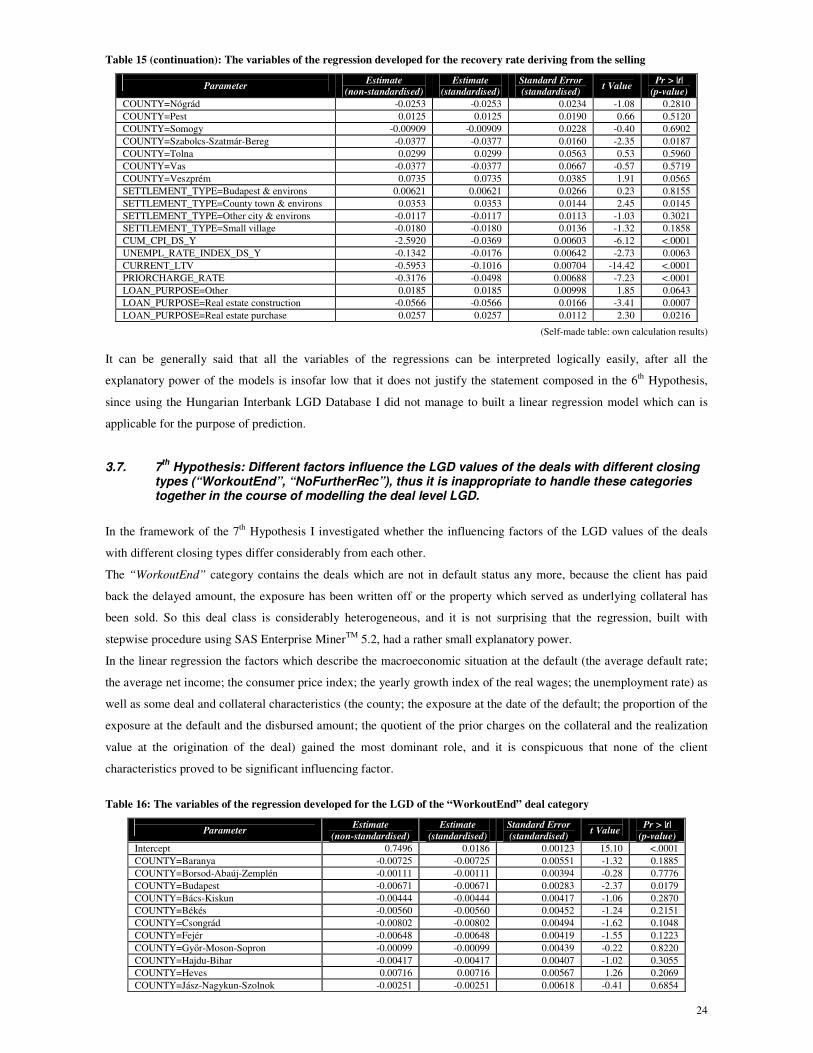
24

Table 15 (continuation): The variables of the regression developed for the recovery rate deriving from the selling

Parameter Estimate



t Value Pr > |t|

(p-value)

COUNTY=Nógrád -0.0253 -0.0253 0.0234 -1.08 0.2810 COUNTY=Pest 0.0125 0.0125 0.0190 0.66 0.5120 COUNTY=Somogy -0.00909 -0.00909 0.0228 -0.40 0.6902 COUNTY=Szabolcs-Szatmár-Bereg -0.0377 -0.0377 0.0160 -2.35 0.0187 COUNTY=Tolna 0.0299 0.0299 0.0563 0.53 0.5960 COUNTY=Vas -0.0377 -0.0377 0.0667 -0.57 0.5719 COUNTY=Veszprém 0.0735 0.0735 0.0385 1.91 0.0565 SETTLEMENT_TYPE=Budapest & environs 0.00621 0.00621 0.0266 0.23 0.8155 SETTLEMENT_TYPE=County town & environs 0.0353 0.0353 0.0144 2.45 0.0145 SETTLEMENT_TYPE=Other city & environs -0.0117 -0.0117 0.0113 -1.03 0.3021 SETTLEMENT_TYPE=Small village -0.0180 -0.0180 0.0136 -1.32 0.1858 CUM_CPI_DS_Y -2.5920 -0.0369 0.00603 -6.12 <.0001 UNEMPL_RATE_INDEX_DS_Y -0.1342 -0.0176 0.00642 -2.73 0.0063 CURRENT_LTV -0.5953 -0.1016 0.00704 -14.42 <.0001 PRIORCHARGE_RATE -0.3176 -0.0498 0.00688 -7.23 <.0001 LOAN_PURPOSE=Other 0.0185 0.0185 0.00998 1.85 0.0643 LOAN_PURPOSE=Real estate construction -0.0566 -0.0566 0.0166 -3.41 0.0007 LOAN_PURPOSE=Real estate purchase 0.0257 0.0257 0.0112 2.30 0.0216

(Self-made table: own calculation results) It can be generally said that all the variables of the regressions can be interpreted logically easily, after all the

explanatory power of the models is insofar low that it does not justify the statement composed in the 6th Hypothesis,

since using the Hungarian Interbank LGD Database I did not manage to built a linear regression model which can is

applicable for the purpose of prediction.

3.7. 7th

Hypothesis: Different factors influence the LGD values of the deals with different closing types (“WorkoutEnd”, “NoFurtherRec”), thus it is inappropriate to handle these categories together in the course of modelling the deal level LGD.

In the framework of the 7th Hypothesis I investigated whether the influencing factors of the LGD values of the deals

with different closing types differ considerably from each other.

The “WorkoutEnd” category contains the deals which are not in default status any more, because the client has paid

back the delayed amount, the exposure has been written off or the property which served as underlying collateral has

been sold. So this deal class is considerably heterogeneous, and it is not surprising that the regression, built with

stepwise procedure using SAS Enterprise MinerTM 5.2, had a rather small explanatory power.

In the linear regression the factors which describe the macroeconomic situation at the default (the average default rate;

the average net income; the consumer price index; the yearly growth index of the real wages; the unemployment rate) as

well as some deal and collateral characteristics (the county; the exposure at the date of the default; the proportion of the

exposure at the default and the disbursed amount; the quotient of the prior charges on the collateral and the realization

value at the origination of the deal) gained the most dominant role, and it is conspicuous that none of the client

characteristics proved to be significant influencing factor.

Table 16: The variables of the regression developed for the LGD of the “WorkoutEnd” deal category

Parameter Estimate

(non-standardised)

Estimate

(standardised)

Standard Error

(standardised)

t Value Pr > |t|

(p-value)

Intercept 0.7496 0.0186 0.00123 15.10 <.0001 COUNTY=Baranya -0.00725 -0.00725 0.00551 -1.32 0.1885 COUNTY=Borsod-Abaúj-Zemplén -0.00111 -0.00111 0.00394 -0.28 0.7776 COUNTY=Budapest -0.00671 -0.00671 0.00283 -2.37 0.0179 COUNTY=Bács-Kiskun -0.00444 -0.00444 0.00417 -1.06 0.2870 COUNTY=Békés -0.00560 -0.00560 0.00452 -1.24 0.2151 COUNTY=Csongrád -0.00802 -0.00802 0.00494 -1.62 0.1048 COUNTY=Fejér -0.00648 -0.00648 0.00419 -1.55 0.1223 COUNTY=Győr-Moson-Sopron -0.00099 -0.00099 0.00439 -0.22 0.8220 COUNTY=Hajdu-Bihar -0.00417 -0.00417 0.00407 -1.02 0.3055 COUNTY=Heves 0.00716 0.00716 0.00567 1.26 0.2069 COUNTY=Jász-Nagykun-Szolnok -0.00251 -0.00251 0.00618 -0.41 0.6854

25

Table 16 (continuation): The variables of the regression developed for the LGD of the “WorkoutEnd” deal category

Parameter Estimate



t Value Pr > |t|

(p-value)

COUNTY=Komárom-Esztergom -0.00220 -0.00220 0.00409 -0.54 0.5914 COUNTY=Nógrád 0.00510 0.00510 0.00584 -0.87 0.3824 COUNTY=Pest -0.00101 -0.00101 0.00290 -0.35 0.7277 COUNTY=Somogy -0.00658 -0.00658 0.00683 -0.96 0.3354 COUNTY=Szabolcs-Szatmár-Bereg -0.00509 -0.00509 0.00384 -1.33 0.1847 COUNTY=Tolna 0.0169 0.0169 0.00831 2.03 0.0421 COUNTY=Vas -0.00375 -0.00375 0.00708 -0.53 0.5965 COUNTY=Veszprém -0.00213 -0.00213 0.00400 -0.53 0.5947 DEFAULTED_EXPOSURE_LCY 5.28E-10 0.00275 0.00101 2.72 0.0065 DEFAULTED_PER_START_EXPOSURE 0.0216 0.00399 0.00122 3.27 0.0011 PRIORCHARGE_RATE 0.0173 0.00250 0.000973 2.57 0.0103 AVG_PD -0.6131 -0.0153 0.00307 -4.97 <.0001 DEFAULT_AVG_NETINCOME -4.08E-7 -0.00349 0.00175 -1.99 0.0464 DEFAULT_CPI -0.5301 -0.00774 0.00130 -5.95 <.0001 DEFAULT_REALWAGE_INDEX -0.1616 -0.00587 0.00108 -5.42 <.0001 DEFAULT_UNEMPL_RATE 0.5051 0.00805 0.00308 2.61 0.0090

(Self-made table: own calculation results) I consider it necessary to emphasize the negative sign of the estimated parameter of the default rate (avg_PD), since we

can usually read in the literature about the positive correlation between the LGD and the default rate (for example

Grunert and Weber [2005], Brady et al. [2007], Bellotti and Crook [2008]), or in some cases about independency

respectively (Carey – Gordy [2003]). However, in case of the other factors the results were not surprising.

The “NoFurtherRec” category consists of the deals which are still in default status, since their becoming non-

performing longer than 36 months duration has passed, and in case of which at least 90% of the exposure at the date of

default has recovered. According to my anticipative expectations, this group is much more homogeneous in comparison

with the “WorkoutEnd” category, and the influencing factors of the deal level LGD can be better defined. This model

proved to be much stronger indeed.

In this linear regression the client characteristics (the age of the client at the default; the landline phone) also played an

important role in addition to the deal and collateral characteristics (the length of the period from the origination of the

deal to the default event; whether the deal became non-performing because of delay; the region; the type of the

settlement) as well as the macroeconomic factors (the growth of the real wages, of the consumer prices and of the GDP

in the period from the origination of the deal to the default; the average default rate at the default date), contrary to the

regression prepared for the “WorkoutEnd” deal category.

Table 17: The variables of the regression developed for the LGD of the “NoFurtherRec” deal category

Parameter Estimate

(non-standardised)

Estimate

(standardised)

Standard Error

(standardised)

t Value Pr > |t|

(p-value)

Intercept -7.9544 0.7094 0.0323 21.96 <.0001 DEFAULT_AGE_MONTHS -0.00018 -0.0251 0.0106 -2.35 0.0190 LINE_PHONE_FLAG=0 0.0209 0.0209 0.0103 2.04 0.0421 REASON_PASTDUE=0 -0.1702 -0.1702 0.0297 -5.72 <.0001 MONTHS_TO_DEFAULT -0.0304 -0.2216 0.0358 -6.20 <.0001 REGION=Budapest & environs -0.0347 -0.0347 0.0388 -0.89 0.3714 REGION=Central-Western -0.0308 -0.0308 0.0283 -1.09 0.2766 REGION=Eastern 0.0284 0.0284 0.0263 1.08 0.2811 REGION=North-Eastern 0.0488 0.0488 0.0198 2.46 0.0142 REGION=North-Western -0.0580 -0.0580 0.0305 -1.90 0.0577 REGION=South-Central 0.0361 0.0361 0.0407 0.89 0.3751 REGION=South-Eastern -0.0347 -0.0347 0.0326 -1.06 0.2878 REGION=South-Western 0.000328 0.000328 0.0422 0.01 0.9938 SETTLEMENT_TYPE=Budapest & environs 0.0253 0.0253 0.0383 0.66 0.5091 SETTLEMENT_TYPE=County town & environs -0.0721 -0.0721 0.0227 -3.17 0.0016 SETTLEMENT_TYPE=Other city & environs 0.00688 0.00688 0.0180 0.38 0.7034 SETTLEMENT_TYPE=Small village 0.0298 0.0298 0.0234 1.27 0.2030 CUM_REALWAGE_INDEX_DS -2.7167 -0.0573 0.0122 -4.70 <.0001 CUM_CPI_DS 2.3466 0.0884 0.0390 2.27 0.0239

26

Table 17 (continuation): The variables of the regression developed for the LGD of the “NoFurtherRec” deal category

Parameter Estimate



t Value Pr > |t|

(p-value)

GDP_GROWTH_INDEX_DS 9.0760 0.1762 0.0148 11.93 <.0001 AVG_PD 3.6371 0.0417 0.0137 3.04 0.0025

(Self-made table: own calculation results) On the basis of the linear regression models developed for the “WorkoutEnd” and the ”NoFurtherRec” deal categories,

it can be said summing up that the results support the statement composed in my 7th Hypothesis according to which

different factors influence the LGD values of the deals with different closing types, thus it is inappropriate to handle

them together in the course of modelling the deal level LGD.

4. Summary: the applicability of the results in practice In the past period the questions in connection with the capital adequacy received high priority for the credit institutions.

All the ingravescent economic problems, the increasing risks and the aggravation of the capital adequacy prescriptions

have the affect that the capital available for the institutions is tighter and tighter. Under such conditions the proper

capital management and portfolio management are essential, thus the exact quantification of the credit risk parameters

also has an increasing importance.

Taking into consideration this aspect as well, the notability of prudential definition of the pooling criteria is undoubted,

since the divergence of the risk parameters results in different capital requirements withal, thus the credit risk

parameters serve as important input factors for the decisions in connection with the portfolio management as well. In

case of the portfolio examined by me I experienced significant differences between the LGD values of the certain

subportfolios in the course of the categorization according to both the purpose of the loan and the type of the

application. Naturally the appropriate pooling criteria can differ from each other institute by institute, moreover they

can change in time as well, thus the dynamic approach and the systematic revisions are essential in the course of their

use. For that matter the CRD prescribes as well that concerning the statistical models comprehensive supervision has to

be made at least annually, which has to include the monitoring of the predictive power, the freeness of distortion and the

stability, the review of specifications, the comparison of predicted and real realized results (Back Testing). For the

objectivity and exploration of the model’s deficiencies the requirement of a review by professional evaluation is a

further prescription (EC [2011c] Article 170; Hkr. 63. §).

The result that the applied discount rate has significant LGD-influencing role is important because actually neither the

CRD nor the national regulation contains particular prescriptions regarding what kind of method the rate should be

defined with. In my opinion the contractual lending rate of the deals can be considered as the most appropriate one,

since it reflects both the differences between the actual interest levels at the date of the origination of certain deals, and

on the other hand it varies according to their currency as well. However, the empirical results indicate that the definition

significantly influences the calculated LGD values.

The appropriate choice of the materiality threshold is generally important, because it promotes the elimination of

numerous technical default events, since therefore the delay of “insignificant amounts” does not result automatically in

getting into non-performing status. On the other hand according to my empirical researches the decision about the

materiality threshold takes notable effect on the calculated value of the risk parameters in case of the mortgage loans as

well, so the opportunity composed in Hkr. 68. § (5)-(7) Paragraph according to which the credit institutions are allowed

to use criteria which are different from the prescriptions has great importance.

In the course of my researches I did not manage to build regression models having so large explanatory power on the

basis of the data of the Hungarian Interbank LGD Database that this way the deals can also be involved in the

calculations whose collection process has not been closed yet, but according to my expectations this will also be

possible later when the quantity of the deals in the database increases. Considering that the use of the data deriving from

27

the common database can provide advantages for all the credit institutions, it would be expediential that more

institutions join it and create a relatively large and variegated database by historic uploading their data, which also

enables the consideration of the individual characteristics of their portfolios applying the proper filters.

Keeping it in view I focused in the framework of my dissertation on the analysis of the categories according to the

closing type of the deals: I examined the differences between the LGD values of the individual groups, the opportunities

of the classification as well as the influencing factors of the LGD values of the certain categories, and all of my results

confirmed my anticipative expectations according to which the separate handling of these groups is reasonable. I

managed to build a logistic regression with which the futural closing type of the deals with not yet closed collection

process can also be predicted with quite great reliability, thus I count great potential to the data of the Hungarian

Interbank LGD Database concerning its futural use in the predictions regarding the recovery rates from collateral

selling.

28

5. Main references

ALLISON, P. D. [1998]: Survival Analysis Using SAS: A Practical Guide, SAS Publishing ALTMAN, E. I. [2009]: Default Recovery Rates and LGD in Credit Risk Modeling and Practice: An Updated Review of

the Literature and Empirical Evidence. Working Paper, New York University, Stern School of Business ALTMAN, E. I. – RESTI, A. – SIRONI, A. [2005b]: Loss Given Default: A Review of the Literature. In: ALTMAN, E. I. –

RESTI, A. – SIRONI, A. (eds.): Recovery Risk. The Next Challenge in Credit Risk Management. Risk Books, London. NYU Salomon Center and NYU Stern School of Business; Bocconi University, pp. 41-59.

BARTLETT, M. S. [1996]: Multivariate Analysis. Journal of the Royal Statistical Society, Series B, Vol. 9, pp. 176-197. BELLOTTI, T. – CROOK, J. [2009]: Calculating LGD for credit cards. GFRMC Conference on Risk Management in the

Personal Financial Services Sector. London BHATIA, M. [2006]: Credit Risk Management & Basel II. – An Implication Guide. Risk Books, Navarra BRADY, B. – CHANG, P. – MIU, P. – OZDEMIR, B. – SCHWARTZ, D. C. [2007]: Discount Rate for Workout Recoveries: An

Empirical Study. Social Science Research Network, Working Paper Series, August CALEM, P. S. – LACOUR-LITTLE, M. [2004]: Risk-Based Capital Requirements for Mortgage Loans. Journal of Banking

& Finance, Vol. 28, pp. 647-672. CAREY, M. – GORDY, M. [2003]: Systematic Risk in Recoveries on Defaulted Debt. Mimeo, Federal Reserve Board,

Washington, DC CLAURETIE, T. M. [1990]: A Note on Mortgage Risk: Default vs. Loss Rate. EREZEA Journal, Vol. 18, No. 2, pp. 202-

206. CLAURETIE, T. M. – HERZOG, T. [1990]: The Effect of State Foreclosure Laws on Loan Losses: Evidence form

Mortgage Insurance Industry. Journal of Money, Credit, and Banking, Vol. 22, No. 2, pp. 221-233. COX, D. R. [1984]: Analysis of Survival Data. Chapman & Hall, London CROUHY, M – GALAI, D. – MARK, R. [2001]: Risk Management. McGraw-Hill, New York DE LAROSIÈRE, J. [2009]: The High-level group on financial supervision in the EU: Report. Brussels, 25th February

2009. URL: http://ec.europa.eu/internal_market/finances/docs/de_larosiere_report_en.pdf (downloaded: 25.07.2011.)

DE SERVIGNY, A. – OLIVER, R. [2004]: Measuring and Managing Credit Risk. McGraw Hill, Boston DERKSEN, S. – KESELMAN, J. H. [1992]: Backward, Forward, and Stepwise Automated Subset Selection Algorithms.

Frequency of Obtaining Authentic and Noise Variables. British Journal of Mathematical and Statistical Psychology, Vol. 45, pp. 265-282.

DERMINE, J. – NETO DE CARVALHO, C. [2005]: How to Measure Recoveries and Provisions on Bank Lending: Methodology and Empirical Evidence. In: ALTMAN, E. I. – RESTI, A. – SIRONI, A. (eds.): Recovery Risk. The Next Challenge in Credit Risk Management. Risk Books, London. NYU Salomon Center and NYU Stern School of Business; Bocconi University, pp. 101-119.

DRAPER, N. – SMITH, H. [1981]: Applied Regression Analysis. John Wiley & Sons, Inc., New York EC [2011a]: Proposal for a Directive of the European Parliament and of the Council on credit agreements relating to

residential property. European Commission, Brussels, 31st March 2011. URL: http://www.europolitics.info/pdf/gratuit_en/291224-en.pdf (downloaded: 10.08.2011.)

EC [2011c]: Proposal for a Regulation of the European Parliament and of the Council on prudential requirements for credit institutions and investment firms. European Commission, Brussels, 20th July 2011. URL: http://ec.europa.eu/internal_market/bank/docs/regcapital/CRD4_reform/20110720_regulation_proposal_part1_en.pdf; http://ec.europa.eu/internal_market/bank/docs/regcapital/CRD4_reform/20110720_regulation_proposal_part2_en.pdf; http://ec.europa.eu/internal_market/bank/docs/regcapital/CRD4_reform/20110720_regulation_proposal_part3_en.pdf (downloaded: 31.07.2011.)

EC [2011d]: Proposal for a Directive of the European Parliament and of the Council on the access to the activity of credit institutions and the prudential supervision of credit institutions and investment firms and amending Directive 2002/87/EC of the European Parliament and of the Council on the supplementary supervision of credit institutions, insurance undertakings and investment firms in a financial conglomerate. European Commission, Brussels, 20th July 2011. URL: http://eur-lex.europa.eu/LexUriServ/LexUriServ.do?uri=COM:2011:0453:FIN:EN:PDF (downloaded: 31.07.2011.)

ENGELMANN, B. – RAUHMEIER, R. (eds.) [2006]: The Basel II Risk Parameters. Estimation, Validation, and Stress Testing. Springer Verlag, Heidelberg/Berlin

EPC [2006a]: Directive 2006/48/EC of the European Parliament and of the Council of 14th June 2006 relating to the taking up and pursuit of the business of credit institutions (recast). European Parliament and of the Council, Official Journal of the European Union L177, 30th June 2006

EPC [2006b]: Directive 2006/49/EC of the European Parliament and of the Council of 14th June 2006 on the capital adequacy of investment firms and credit institutions (recast). European Parliament and of the Council, Official Journal of the European Union L177, 30th June 2006

FÜSTÖS, L. – KOVÁCS, E. – MESZÉNA, GY. – SIMONNÉ, M. N. [2004]: Alakfelismerés. Sokváltozós statisztikai módszerek. (Pattern Recognition. Multivariate Statistical Methods) Új Mandátum Kiadó, Budapest

GREENE, W. H. [2003]: Econometric Analysis. 5th Edition (International student), Prentice Hall, New Jersey GRIPPA, P. S. – IANNOTTI, F. – LEANDRI, F. [2005]: Recovery rates in the banking industry: stylised facts emerging from

the Italian experience. In: ALTMAN, E. I. – RESTI, A. – SIRONA, A. (eds.): Recovery Risk. Risk Books, London, pp. 121-141.

29

GRUNERT, J. – WEBER, M. [2005]: Recovery Rates of Bank Loans: Empirical Evidence for Germany. Department of Banking and Finance, University of Mannheim, Working Paper, March

HAJDU, O. [2003]: Többváltozós statisztikai számítások. Statisztikai módszerek a társadalmi és gazdasági elemzésekben. (Multivariate Statistical Calculations. Statistical Methods in the Social and Economic Analyses) Központi Statisztikai Hivatal (Hungarian Central Statistical Office), Budapest

HAJDU, O. (ed.) [2004]: Statisztika III. (Statistics III) Egyetemi jegyzet, Budapest HAMILTON, D. T. – VARMA, P. – OU, S. – CANTOR, R. [2003]: Loss. Characteristics of Commercial Mortgage

Foreclosure HARREL, F. E. [2001]: Regression Modeling Strategies: With Applications to Linear Models, Logistic Regression, and

Survival Analysis. Springer Series in Statistics. Springer-Verlag, New York HFSA [2008c]: Validációs Kézikönyv. A belső minősítésen alapuló módszerek és a működési kockázat fejlett mérési

módszereinek (AMA) bevezetéséről, értékeléséről, jóváhagyásáról. I. rész: A belső minősítésen alapuló módszer. (Validation Guidelines. On the implementation, assessment and approval of Internal Ratings Based (IRB) Approaches and Advanced Measurement Approaches (AMA). Part I: International Ratings Based Approach.) Pénzügyi Szervezetek Állami Felügyelete (Hungarian Financial Supervisory Authority), June

HFSA [2010]: A hitelintézetek és befektetési vállalkozások tőkekövetelmény szabályozásának (CRD) a közelmúltban elfogadott és jelenleg folyamatban lévő uniós módosításai. (The Union’s Recently Accepted or Actually Ongoing Modifications of the Capital Requirement Regulation of Credit Institutions and Investment Firms (CRD)) Pénzügyi Szervezete Állami Felügyelete (Hungarian Financial Supervisory Authority). URL: http://www.pszaf.hu/data/cms2109746/CRD_I_IV_aktualizalt_internetre.pdf (downloaded: 25.07.2010.)

HMA [2008]: LGD-adatbázis rendszerterv. (LGD Database System plan) Magyar Jelzálogbank Egyesület (Hungarian Mortgage Association), 7th March 2008

HUNYADI, L. – VITA, L. [2004]: Statisztika közgazdászoknak. Statisztikai módszerek a társadalmi és gazdasági elemzésekben. (Statistics for Economists. Statistical Methods in the Social and Economic Analyses) 3rd Edition, Központi Statisztikai Hivatal (Hungarian Central Statistical Office), Budapest

INFO-DATAX [2006]: Összbanki LGD adatbázis adatmodellje. (Data Model of the Interbank LGD Database). Info-Datax Kft., July 2006

KARDOSNÉ, V. ZS. [2010]: Várható változások az európai tőkeszabályozásban. (Expected Changes in the European Capital Regulation) Hitelintézeti Szemle, Vol. 9, No. 3, pp. 236-248.

KLEINBAUM, D. G. – KUPPER, L. L. – MULLER, K. E. – NIZAM, A. [1998]: Applied Regression Analyis and Other Multivariable Methods. 3rd Edition, Brooks/Cole Publishing Company, Duxbury Press, pp. 656-686.

KLUGMAN, S. A. – PANJER, H. H. – WILLMOT, G. E. [2008]: Loss Models. From Data to Decisions. 3rd Edition, John Wiley & Sons, Inc., New Jersey

LEKKAS, V. – QUIGLEY, J. M. – VAN ORDER, R. [1993]: Loan Loss Severity and Optimal Mortgage Default. Journal of

the American Real Estate and Urban Economics Association, Vol. 21, No. 4, pp. 353-371. MACKINNON, J. G. [1992]: Model Specification Tests and Artificial Regression. Journal of Economic Literature, Vol.

30, pp. 102-145. MACLACHLAN, I. [2005]: Choosing the Discount Factor for Estimating Economic LGD. In: ALTMAN, E. I. – RESTI, A. –

SIRONI, A. (eds.): Recovery Risk. The Next Challenge in Credit Risk Management. Risk Books, London, pp. 285-305.

MADDALA, G. S. [2004]: Bevezetés az ökonometriába (Introduction to Econometrics). Nemzetközi Tankönyvkiadó, Budapest. Source: MADDALA, G. S. [2001]: Introduction to Econometrics, John Wiley & Sons, Ltd.

MELNICK, E. L. – EVERITT, B. S. (eds.) [2008]: Encyclopedia of Quantitative Risk Analysis and Assessment. John Wiley & Sons, Inc.

MORAL, G. – GARCÍA-BAENA, R. [2002]: LGD Estimates in a Mortgage Portfolio. Estabilidad Financiera, Banco de España, Vol. 3, pp. 127–164. (Financial Stability Review)

MORAL, G. – OROZ, M. [2002]: Interest Rates and LGD Estimates. Manuscript NELDER, J. A. – WEDDERBURN, R. W. [1972]: Generalized linear models. Journal of the Royal Statistical Society, Series

A, Vol. 135, No. 3, pp. 370-384. PAULOVICS, O. [2005]: LGD modellezés elméletben és gyakorlatban. (LGD Modelling in Theory and in Practice)

Hitelintézeti Szemle, Vol. 4, No. 5-6, pp. 63-83. QI, M. – YANG, X. [2009]: Loss Given Default of High Loan-to-value Residential Mortgages. Risk Management

Research Report, Journal of Banking & Finance, 33, pp. 788-799. (QI, M. – YANG, X. [2007]: Loss Given Default of High Loan-to-value Residential Mortgages. Economics and Policy Analysis working Paper, No. 4, August)

RAMANATHAN, R. [2003]: Bevezetés az ökonometriába, alkalmazásokkal. (Introductory Econometrics with Applications) Panem Kiadó, Budapest. (Source: RAMANATHAN, R. [2002]: Introductory Econometrics with Applications. 5th Edition, Harcourt College Publishers, New York)

THOMAS, L. C. – MATUSZYK, A. – MOORE, A. [2007a]: Collections policy comparison in LGD modelling. 3rd September, URL: http://www.management.soton.ac.uk/research/publications/CRR-09-03.pdf (downloaded: 09.08.2010.)

WITTEN, I. H. – FRANK, E. [2005]: Data Mining. Practical Machine Learning Tools and Techniques. 2nd Edition, Elsevier, Morgan Kaufmann Publishers, Inc.

WOOLDRIDGE, J. M. [2009]: Introductory Econometrics: A modern approach. 4th Edition, South-Western Act CXII of 1996 on Credit Institutions and Financial Enterprises (Hpt.) Government Decree No. 196/2007 on the Management and Capital Requirement of Credit Risk (Hkr.)

30

6. Own publications in connection with the topic 6.1. Articles in Journals (in Hungarian)

ZSUZSANNA TAJTI [2005]: A modernkori bankbiztosítás magyarországi története. (The Hungarian History of the Modern Bankassurance) Hitelintézeti Szemle, Vol. 4, No. 2, pp. 57-73.

ZSUZSANNA TAJTI [2005]: Egy kombinált bankbiztosítási jelzáloghitel-konstrukció elemzése.

(Analysis of a Combined Bankassurance Mortgage Loan Construction) Hitelintézeti Szemle, Vol. 4, No. 4, pp. 37-64.

ZSUZSANNA TAJTI [2011]: A bázeli ajánlások és a tőkemegfelelési direktíva (CRD) formálódása.

(Changes of the Basel Recommendations and of the Capital Adequacy Directive (CRD)) Hitelintézeti Szemle, Vol. 10, No. 5, pp. 499-519.

6.2. E-learning Curriculum (in Hungarian)

ZSUZSANNA TAJTI [2008]: Banküzemtan – Vállalkozások bankkapcsolatai. (Banking – Relationships between the Enterprises and the Banks) Kodolányi János Főiskola

6.3. Conference Presentation and Article in Conference Paper (in English)

ZSUZSANNA TAJTI [2010]: An application of historical internal and external data for loss given default calculation. 7th International Conference of PhD Students, University of Miskolc, 8-12th August, pp. 131-136.

6.4. Book (in English)

ZSUZSANNA TAJTI [under discussion]: The methodological opportunities of quantifying the retail mortgage loan LGD in Hungary. LAP LAMBERT Academic Publishing GmbH & Co. KG, Germany, Saarbrücken

collection of theses zsuzsanna tajti

Documents