collective atomic recoil laser as a synchronization transition · collective atomic recoil laser as...

Collective atomic recoil laser as a synchronization transition

J. JavaloyesInstitut Mediterrani d’Estudis Avançats (IMEDEA), Campus Universitat de les Illes Balears, E-07122 Palma de Mallorca, Spain

M. PerrinLaboratoire de Physique des Lasers Atomes et Molécules, F-59655 Villeneuve d’Ascq Cedex, France

and Max-Planck-Institut fur Physik Komplexer Systeme, Nothnitzer Strasse 38, D-01187 Dresden, Germany

A PolitiIstituto dei Sistemi Complessi, CNR, via Madonna del Piano 10, I-50019 Sesto Fiorentino, Italy

�Received 10 December 2007; published 8 July 2008�

We consider here a model previously introduced to describe the collective behavior of an ensemble of coldatoms interacting with a coherent electromagnetic field. The atomic motion along the self-generated spatiallyperiodic force field can be interpreted as the rotation of a phase oscillator. This suggests a relationship withsynchronization transitions occurring in globally coupled rotators. In fact, we show that whenever the fielddynamics can be adiabatically eliminated, the model reduces to a self-consistent equation for the probabilitydistribution of the atomic “phases.” In this limit, there exists a formal equivalence with the Kuramoto model,though with important differences in the self-consistency conditions. Depending on the field-cavity detuning,we show that the onset of synchronized behavior may occur through either a first- or second-order phasetransition. Furthermore, we find a secondary threshold, above which a periodic self-pulsing regime sets in, thatis immediately followed by the unlocking of the forward-field frequency. At yet higher, but still experimentallymeaningful, input intensities, irregular, chaotic oscillations may eventually appear. Finally, we derive a simplermodel, involving only five scalar variables, which is able to reproduce the entire phenomenology exhibited bythe original model.

DOI: 10.1103/PhysRevE.78.011108 PACS number�s�: 05.90.�m, 42.65.Sf, 42.50.Wk, 05.45.Xt

I. INTRODUCTION

Much progress has been recently made in understandingthe onset of collective phenomena in cold atoms in the pres-ence of a coherent electromagnetic field, when atomic recoilcannot be neglected. In particular, the experimental observa-tion of collective atomic recoil laser �CARL� �1�, accompa-nied by the development of simple theoretical models �2�,has revealed that this is an appropriate physical environmentfor testing new and general ideas on the behavior of globallycoupled oscillators. In fact, the position of an atom movingalong a line in a self-generated periodic potential can beinterpreted as a phase: this observation opens up the possi-bility to compare CARL with other globally coupled systems�3–5� and, in particular, with the Kuramoto model �KM� �6�.It is also interesting to explore the formal analogy with neu-ral networks, which are currently the object of a strong re-search activity �see, e.g., �7,8�� in the perspective of unrav-eling the underlying information processing mechanisms. Infact, in one of the simplest, although nontrivial, modelingschemes, neurons can be assimilated to rotators, since theaction potential can be interpreted as a phase �this is, e.g., thecase of the so called “leaky integrate and fire” neurons �LIF��7��. One of the goals of this manuscript is precisely to in-vestigate analogies and differences between the collectivephenomena that can arise in cold atoms and the synchroni-zation phenomena that occur in general models of globallycoupled rotators.

Altogether, the idea of atomic recoil is often linked withoptical cooling �9�, but several years ago it was suggestedthat the recoil resulting from photon emission or absorption

could induce macroscopic phenomena �2� and possibly con-tribute to the transformation of kinetic energy into coherentlight emission, in analogy to what happens in the free elec-tron laser �10�.

However, for a long time, progress on the theoretical sidewas hindered by the lack of a suitable model to describe theasymptotic stationary behavior of an ensemble of atoms. Pre-liminary experiments conducted at room temperature �11,12�were also partially inconclusive, as pointed out in �13�. As aconsequence, it was unclear which experimental conditionswould be more appropriate for an experimental observationand even whether collective phenomena could be seen at all.

With the introduction of the first model capable of ac-counting for stationary phenomena �14�, it has been shownthat at sufficiently low temperatures �above the region wherequantum effects become important� an atomic-polarizationgrid can spontaneously arise, which triggers a coherent back-propagating field �15�. More recently, experimental evidencehas been found �1� and a corresponding theory has been pro-posed �16–18�, of collective atomic recoil lasing action in thepresence of a very strong detuning, when the atomic dynam-ics can be effectively described by a linear response theory.Although a density grating arises in both cases, it is only inthe latter setup that it contributes to generating the back-propagating field, while in the former one it just followsfrom the existence of two counterpropagating fields and it isnot the dominant mechanism providing self-amplification.

So far, the only collective behavior that has been observedis the spontaneous onset of a slightly detuned backward-propagating constant field through a second order transition.In this paper, we extend the theoretical study, by first show-

PHYSICAL REVIEW E 78, 011108 �2008�

1539-3755/2008/78�1�/011108�13� ©2008 The American Physical Society011108-1

http://dx.doi.org/10.1103/PhysRevE.78.011108

ing that the phase of the backward field can be eliminated byreferring to a frame that moves with the instantaneous back-ward field frequency. This step allows uncovering an analogywith the KM, but also some relevant differences. In bothCARL and KM, the force fields are self-consistently gener-ated and depend on the nonuniformity in the probability dis-tribution; moreover, both of them contain a mean-field sinu-soidal term that eventually triggers ferromagnetic ordering.However, at variance with the “standard” KM, the slope ofthe potential �i.e., the effective frequency of the oscillators�is self-generated and there exists a preferred moving frame�the one we have accurately selected� where the dynamics isautonomous. This makes it meaningful to distinguish be-tween locking �i.e., perfect synchrony� and libration, depend-ing whether the potential exhibits local minima or not. Theunavoidable presence of thermal noise introduces a furtherinteresting effect, namely, a mismatch between the averagevelocity of the atoms and that of the density grating. Thisindeed represents the starting point for establishing a connec-tion with another transition �see below�.

By exploring the behavior for larger but still experimen-tally accessible input intensities �1�, we uncover an unex-pectedly rich bifurcation scenario, starting from the primarytransition which appears to be either second or first order,depending on the magnitude of the detuning between theinjected field and the nearest cavity mode. More interestingis the secondary instability, which gives rise to amplitudeoscillations of both the backward and forward field and isthen followed by an unlocking transition, where the forward-field frequency too starts to be �red� detuned with respect tothe input field. On the one hand, this regime is reminiscent ofthe periodic collective motion predicted in a model of chargedensity waves �4�, but it also resembles “self-organized”quasiperiodicity, a phenomenon first found in a model of LIFneurons �19�, revisited in �20�, and proved in its full gener-ality in �21�. We show that all these features and the transi-tion to chaotic behavior observed for yet higher input inten-sities are captured by a simple model containing only fivevariables. Such a model is derived in the limit of a strongcooperation parameter �see the next section for its definition�and weak dipolar coupling, when the probability density iswell approximated by the first Fourier mode. However, itsvalidity appears to extend to a wide parameter region. Thesimplified model proves useful also to unravel the nature ofthe primary transition in the presence of a nonzero cavity-field detuning.

The paper is organized as follows: In Sec. II, we derivethe explicit form of the self-consistent washboard potentialacting on the particle probability density and discuss theanalogies with the Kuramoto model. In Sec. III, we provide afull characterization of the various dynamical regimes ap-pearing in this model. In Sec. V, we derive a minimal modelconsisting of five ordinary differential equations, that is ableto reproduce the rich phenomenology of the full system. Fi-nally, in Sec. VI, we summarize the main results and com-ment about the open problems.

II. THE MODEL

The original CARL model �2� considers only the dynam-ics of the back-scattered field. Such an approximation is

valid in the vicinity of the first threshold, but it fails at higherinput intensities. It becomes then necessary to consider theforward mode dynamics as well, as first proposed in �22� andfurther discussed in �23,24�. Besides, as analyzed in �16�,different models should be invoked, depending on the physi-cal mechanisms that are responsible for atomic thermaliza-tion. For instance, if the process involves collisions �witheither an external buffer gas, or hard boundaries�, a Vlasovequation with a BGK-type collisional operator �25� for theatomic density in phase space �26� is appropriate to modelthe thermalization. This leads to a Vlasov-type equation forthe evolution of the density of probability. On the other hand,in the context of cold atoms dynamics, thermalization can beachieved via Doppler cooling �27�. Then, each cooling cyclechanges slightly the atomic momentum, and the appropriatethermalization model, as shown in �9�, may therefore be aFokker-Planck operator �28�, to describe the interaction be-tween the probability distribution of particles and the molas-ses fields.

In this latter case, the model consists of a set of twoequations for the complex cavity fields xb, xf, coupled to aFokker-Planck equation for the single particle probabilitydistribution Q�� , p� for the atomic position � and momentump. As in Ref. �16�, we limit ourselves to considering thestrong friction limit, which is both physically meaningful andallows us to obtain some analytical results.

Accordingly, under the simplifying hypothesis of a van-ishingly small inertia, the model reduces to a Fokker-Planckequation for the density ��u , t� of atoms in the position u,accompanied by two equations for the complex amplitudesxf, xb of the forward and backward field, respectively,

�t� = − ��uIm�xfxb�e2iu�� + T�u

2� ,

dxf

dt= − ��1 + i��xf + �Y − i�Cxb�e−2iu� ,

dxb

dt= − ��1 + i��xb − i�Cxf�e2iu� , �1�

where the adimensional parameters have the followingmeaning: �i� C is the atom-field coupling constant; �ii� � isthe suitably shifted �forward� field-cavity detuning; �iii� � isthe dipolar coupling; �iv� T is the atomic temperature; �v� Yis the input field amplitude; �vi� �−1 is the photon lifetimewithin the ring cavity, rescaled to the coherence time of theatomic transition.

We find it convenient to further rescale the variables, intot=�t, xf =YF, xb=YB, and u=z /2 �which implies ��u , t�=2P�z , t��. Accordingly, the model reads

�tP = − ��zIm�FB�eiz�P + ��z2P ,

F = − �1 + i��F + 1 − iCBR�,

B = − �1 + i��B − iCFR , �2�

JAVALOYES, PERRIN, AND POLITI PHYSICAL REVIEW E 78, 011108 �2008�

011108-2

where the dot denotes the derivative with respect to the newtime variable t, and we have explicitly introduced the orderparameter,

R�t� = �0

2

dzeizP�z,t� . �3�

Moreover, we defined the two effective control parameters�=2Y2� /� and �=4T /�. As a result, it turns out that thereare four relevant parameters that cannot be scaled out,namely, the detuning �, the so-called cooperation parameterC, the input intensity �, and the temperature �.

A. A moving frame

Next, we perform yet another change of variables to re-move an irrelevant variable �a phase� from the dynamics. Wedo that by referring to a moving frame

� = z + �t� , �4�

where is to be defined. The new probability density writes

Q��,t� = P�z,t� . �5�

Additionally, we introduce an amplitude-and-phase descrip-tion for the two fields,

F = fei�,

B = bei�.

Notice that with these notations, a positive �negative� lineargrowth of the phases is to be interpreted as a redshift �blue-shift� in the field frequency. Accordingly, the Fokker-Planckequation reads

�tQ = − �� + �fb sin�� − � − + ��Q + ��2Q .

This equation suggests defining

� � − � . �6�

By doing so, we obtain

�tQ = − �� − � + �fb sin ��Q + ��2Q . �7�

Moreover, the order parameter writes

R = ei��−��Rei �8�

where

Rei � Rc + iRs =� d�ei�Q��,t� . �9�

As a result, the field equations write as

f = cos � − f − CbRs, �10�

b = − b + CfRs, �11�

� = −sin �

f−

CbRc

f− � , �12�

� = −CfRc

b− � . �13�

We can now replace the expression for � and � in theFokker-Planck equation to finally obtain

�tQ = − ��Cf2 − b2

fbRc −

sin �

f+ �fb sin �Q + ��

2Q ,

�14�

from which we see that the variable � does not play any rolein the dynamics, since it does not contribute to any of theforce fields. Accordingly, we conclude that the model is fullydescribed by the three Eqs. �10�–�12� plus the Fokker-Planckequation �14�. Upon interpreting � as a phase, we can recog-nize atoms as rotators and the underlying dynamics as that ofidentical globally coupled rotators in the presence of noise.The mutual interaction is mediated by the two fields F and Bwhich follow their own dynamics. The primary interest inthis setup was motivated by the possible existence of a re-gime where the modulus of the order parameter �as well asthe amplitude of the backward field� is different from zero.In view of the above relationship with rotator systems, theonset of this regime is akin to a synchronization transition.However, it is also interesting to notice some analogies withthe standard laser threshold. In fact, in both cases the fre-quency of the backward field is self-generated by the dynam-ics, but the corresponding phase does not contribute to thedynamics itself. Accordingly, from a mathematical point ofview, the transition appears to be a degenerate Hopf bifurca-tion. Moreover, from the above equations, it turns out thatthe reference frame moves with a velocity equal to the fre-quency difference between the two fields. In dimensional

variables this means that the frame velocity is 2��− �� /k,where k is the wave number of the injected field.

B. The physical parameter range

In order to keep contact with a possible experimental con-firmation, we give here the meaningful orders of magnitudeof the four relevant parameters, making reference to the ex-periment carried out in Ref. �1�. The cavity is characterizedby a power transmission coefficient of the cavity mirrors T=6.3�10−6 and a roundtrip length �=8.5 cm. Accordingly,the cavity linewidth is �=−c /� ln�R��22 kHz. The atomicsample consists of 85Rb atoms whose temperature and den-sity are T0=250 �K and n=3�1017 m−3, respectively. Thecharacteristic length of the atomic sample is L=10−3 m. Theoptical parameters are given by the coherence dephasing rateof the D1 transition, namely, 2��=�� =5.9 MHz. The dipo-lar moment is D=1.5�10−29 cm−1. The detunings betweenthe injected field and both the atomic transition and the near-est cavity mode are �a=1 THz and �c�0, respectively.Therefore the physical expressions and the relative orders ofmagnitude of the parameters are

C =L

T� O�1 − 102� ,

� = �c + C � � O�0 − 10� ,

COLLECTIVE ATOMIC RECOIL LASER AS A … PHYSICAL REVIEW E 78, 011108 �2008�

011108-3

� =k2kBT0

m�2��2 � O�10−1 − 101� ,

� =Y2��

2�K2�a� O�0 − 10� ,

where is the unsaturated absorption rate per unit length, kBis the Boltzmann constant, and m the atomic mass.

III. STATIONARY STATES

Both in the perspective of determining the stationary so-lution and to emphasize the analogies with the KM, we de-rive an adiabatic CARL model �ACM� by setting the timederivatives of the three field variables equal to zero. In orderto keep the notations as simple as possible, initially we as-sume �=0 �see Sec. V for the qualitative changes induced bya nonzero detuning�. From Eq. �11�

b = CRs f . �15�

By then setting to zero the derivative in Eq. �12�, we obtain

sin � = − C2fRsRc, �16�

while, from Eq. �10�,

cos � = f�1 + C2Rs2� . �17�

By combining together these last two equations, one obtains

f−2 = C4Rs2Rc

2 + �1 + C2Rs2�2.

After replacing back into the equation for Q�� , t�, the modelreduces to

�tQ = − ��1 + � sin ��Q + ��2Q , �18�

where

� =Rc

Rs�19�

� =�CRs

2

Rc��1 + C2Rs2�2 + C4Rs

2Rc2�

. �20�

Since the field dynamics is absent, the model resembles atypical Fokker-Planck equation in a static potential, as stud-ied extensively by Risken �28�, except that the force field ishere determined self-consistently from some moments of thedistribution Q. The structure of the force field corresponds tothat of the so-called Adler, or washboard, potential �29�. Theparameters � and �, respectively, measure the tilt and modu-lation amplitude of the potential. The tilt originates from ourchoice of a moving frame: a stationary solution for the prob-ability density would indeed correspond to a moving gratingin the laboratory frame. The second parameter � quantifiesthe amplitude of the entraining force on the atomic could.For ��1, the drifting velocity is simply modulated, but itdoes not change sign. For ��1, the washboard potential pos-sesses a local minimum and complete entrainment �synchro-nization� is possible.

A. The zero temperature limit

In order to understand the underlying physics, it is conve-nient to start from the zero-noise limit. A priori, the two mostsymmetric solutions are �i� the perfectly synchronized statewith all particles located in the same position; �ii� the so-called splay state �30�, characterized by a constant flux ofparticles.

If all particles are located in �, then �Rc ,Rs�= �cos � , sin �� and we can reduce the whole problem to theordinary differential equation,

� =cos �

sin �+

�C sin2 �

1 + C2�2 + C2�sin2 �. �21�

The fixed point solution of the fully synchronized state isobtained by determining the zero of the force field,

cos ��1 + C2�2 + C2�sin2 �� = − �C sin3 � . �22�

By squaring it and introducing X=sin2 �, we obtain the equa-tion

�1 − X��1 + C2�2 + C2�X�2 = �2C2X3. �23�

It is easy to verify that there exists a meaningful solution forany value of the parameters C and �. This means that, atzero temperature, any arbitrarily small input field is able totrigger a backward field that is sufficiently strong to entrainthe atoms in the fully synchronized state.

On the other hand, the splay state is obtained by imposingthat, at zero temperature, the flux is constant, i.e., �� 1+� sin ��Q�=�tQ�0. The probability density then becomesproportional to the inverse of the force field,

Q�� =N

��1 + � sin ��, �24�

where N is a normalization condition. From the definition ofthe order parameter, Eq. �3�, we obtain the condition

Rc + iRs =� d�Nei�

��1 + � sin ��. �25�

By solving the real part of this integral, one easily finds thatRc=0. Accordingly, from Eq. �19�, it follows that �=0 whichmeans that there cannot be any tilt and, as a consequence, nosplay state, because the flux would be necessarily equal tozero.

B. A comparison with the Kuramoto model

At zero temperature, there exists a nontrivial collectivestate for arbitrarily small input field. It is interesting to notethat this regime can be linked to the bad and good cavityregimes discussed in Ref. �17�, where the stationary state ofthe CARL model with an undepleted forward field is consid-ered. From the resulting steady state equations, two distinctscaling laws for the backward field intensity have been foundas a function of the number of particles N, in the limit ofsmall and large cavity losses, where it is proportional to N4/3

and N2, respectively. However, such a limit is not directlyapplicable to our model, since both fields are considered self-


011108-4

consistently. Whether these two regimes can be recovered, atleast in a vicinity of the CARL primary transition, is an openquestion.

At finite temperature, as already shown in Ref. �16�, thereexists a threshold value for the input intensity, below whichthe noise washes out any order. The presence of such a tran-sition as well as the underlying structure of the model arereminiscent of what was observed in the KM. In the absenceof quenched disorder �i.e., assuming that all rotators areidentical�, the KM writes

�tQ = − ��KR sin�� − �Q + ��2Q , �26�

where K denotes the coupling constant, while the other no-tations are the same as before. It is well known that the orderparameter R is larger than zero only if the coupling constantis larger than some critical value which depends on the noisestrength.

From the comparison between the ACM and the KM, onecan notice that the sinusoidal force depends on the localphase in the ACM, while it depends on the phase differencein the KM. This implies that the dynamics of the KM is timeindependent in any moving frame �as long as the velocity isconstant�. It is, nevertheless, convenient to write the evolu-tion equation in the frame which allows removing the driftterm �which is indeed absent in the KM�. On the other hand,the drift term cannot be removed from the ACM withoutintroducing an explicit time dependence. A last differenceconcerns the amplitude of the sinusoidal force which is pro-portional to the order parameter in the KM, while it isstrongly nonlinear, in the ACM, due to the coupling betweenorder parameter and field equations as can be seen in Eqs.�19� and �20�. It is now important to understand the implica-tions of such differences on the observed dynamics, espe-cially in the presence of stochastic processes, when phasetransitions are expected.

C. The type of synchronization

In the vicinity of the primary transition, the backwardfield intensity is arbitrarily small. Therefore � is also a smallquantity and the washboard potential cannot drag the atomiccloud. All the variables being stationary, the flux is constantin the vicinity of the transition, and the collective behavior isa typical splay state. In order to understand how this regimeconnects with the fully synchronous state observed in thezero-noise limit, we solve numerically Eqs. �10�–�12� and

�14� for different temperature values. As illustrated in Fig.1�a�, there is no backward field for large enough �, while theforward field intensity is constant and equal to 1 with ournormalizations. Upon decreasing � below the thresholdvalue, f drops below 1 �dashed line�, while b increases fromzero �solid line� and, at small temperatures, decreases againin this particular case. At the same time, the amplitude of theorder parameter increases monotonously from 0 to 1 �dotdashed line�. Note that the highest backward field does notcorrespond to the most coherent state �R=1�, because of thenonlinear dependence of the potential amplitude on the orderparameter. At the same time, in Fig. 1�b�, we see that fordecreasing �, the relative amplitude � of the modulation in-creases above 1 �meaning that the potential exhibits localminima� and eventually decreases, though remaining largerthan 1 at zero temperature, when there is complete dragging.On the other hand, we see in Fig. 2, that the velocity of thedensity grating, which is given by −� �solid line�, decreasesmonotonously with �. In the same figure, the dashed linecorresponds to the average velocity v of the atoms, that isgiven by

va = − � + 2� , �27�

where � is the stationary flux of the Fokker-Planck equation,

� � �Q�0� − ��Q�0� . �28�

By comparing the two curves, we see that the density gratingvelocity is everywhere larger than the atomic velocity exceptat zero temperature, where the two coincide, the sign of acomplete dragging. The difference is maximal in the vicinityof the primary transition, where the atomic velocity is nearly

0 5 10 15 20σ

0.0

0.2

0.4

0.6

0.8

1.0

b,f,Ra)

0 5 10 15 20σ

0

1

2

3

ξ b)

FIG. 1. �Color online� Left panel: Bifurcationdiagram of the ACM model for �=40, C=5,�=0. Solid, dashed, and dotted-dashed lines cor-respond to b, f , and R as a function of �. Rightpanel: the parameter � of the force field.

0 5 10 15 20σ

0

1

2

3

4

5

-ω , va

FIG. 2. �Color online� Velocity of the density grating �−�, solidline� and average velocity of the atoms �va, dashed line� vs thescaled temperature � and the same parameter values as in Fig. 1.


011108-5

zero �because the backward field is negligible too�, while thegrating velocity is maximal.

In order to check the generality of this scenario, wepresent in Fig. 3 a phase diagram for different values of both� and the input intensity �. There we see that above thetransition line, there are two broad areas that extend down to�=0. In the first one �color-shaded, for larger values of ��,the potential has minima, and there is no fixed point. In thesecond one, �in white, between the transition line and thedashed line�, the potential has no minima. The dashed lineseparating these two regions does not represent a true tran-sition line, but marks a quantitative difference: above �firstregion�, the flux is triggered by the noise, since the barrier tothe right of a minimum is lower than that on the left; below�second region�, the flux is intrinsically deterministic.

IV. NUMERICAL ANALYSIS

So far we have discussed the stationary state that arisesfrom the solution of the ACM. We have shown the existenceof two phases: �i� a trivial one characterized by a zero orderparameter and an independent evolution of the single atoms;�ii� a collective state characterized by two different velocitiesfor the single atoms and the density grating. This scenario issuperficially reminiscent of that one found in the KM, but theproperties of the collective motion are slightly more subtle.In the frame where the dynamics is stationary, there is still anonzero flux induced by a finite tilting that cannot be re-moved. However, there are further differences. At variancewith the KM, here we show the existence of more compli-cated dynamical regimes that appear when the amplitude ofthe injected field is further increased beyond the primarytransition. In Fig. 4, we show the typical sequence of statesthat are detected upon increasing the input field �.

For each value of �, the extrema of the field are plotted.Inside region I, there is only one point, meaning that thecollective state is stationary in the moving frame. A second-ary Hopf bifurcation separates region I from region II, wherethe two field amplitudes start oscillating. In region II,the average frequency of the forward field still remainslocked to that of the input field. This can be appreciated inFigs. 5�a� and 5�d� where we plot the real and imaginarycomponents of the order parameter �Rc, Rs� and of the for-

ward field �fc, fs� for �=2.3. In fact, neither R, nor F exhibitan overall rotation since, in both representations, the limitcycle does not encircle the origin. Upon further increasing �,an unlocking occurs: in region III, the periodic oscillationamplitudes are accompanied by a rotation, as it can be seenin Figs. 5�b� and 5�e�, where both limit cycles projectionsnow encircle the origin for �=6 �see Sec. IV B for details�.Finally, a period doubling bifurcation signals the appearanceof yet more complicated dynamical states and the possibleonset of a chaotic dynamics. This occurs in region IV andcan be appreciated by looking at Figs. 5�c� and 5�f�, wherethe phase state projections are plotted for �=9.

A. The secondary transition

Besides solving directly the Fokker-Planck equation, wehave determined the locus of the secondary Hopf bifurcation,by first determining the steady state in terms of a continued

��

��

0 0.05 0.1 0.15 0.2 0.25σ

0

0.5

1

1.5

2

µ

FIG. 3. �Color online� Phase diagram separating locked or drift-ing from partially locked regimes for C=5.

0

0.5

1.0

b

0 2 4 6 8 10µ

0

0.5

1.0

f

I II III IVa)

b)

FIG. 4. Bifurcation diagram for the backward �a� and forward�b� field amplitudes as a function of �. The other parameters areC=20, �=1, and �=0. The meaning of the various regions is dis-cussed in the text.

-0.1 0Rc

0

0.1Rs

-0.2 0 Rc

-0.2

0

Rs

-0.2 0 0.2Rc

-0.2

0

0.2Rs

0 0.2 fc

0

0.2

0.4fs

0 0.2 fc

-0.2

0

0.2

fs

0 0.2 fc

-0.2

0

0.2

fs

a)

d)

b)

e)

c)

f)

FIG. 5. Phase space portraits of the typical behavior observed inregion II ��a�,�d�, �=2.3�, region III ��b�,�e�, �=6�, and region IV��c�,�f� �=9�. Parameters are those of Fig. 4.


011108-6

fraction expansion as described in �16�. The equilibriumprobability distribution has been evaluated analytically byusing its integral form �see, e.g., �28� for further details�; thestability analysis has been thereby carried out by introducinginfinitesimal perturbations for the fields and for the probabil-ity distribution, by referring to an equispaced mesh contain-ing N�256 points. Finally, we have determined the eigen-values of a sparse Jacobian matrix of size �N+3�2 by meansof the QR decomposition �31� while the integral form of theequilibrium distribution has been evaluated by using theClenshaw-Curtis quadrature integration scheme �32�.

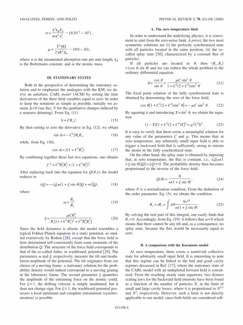
The main results are summarized in Fig. 6. There, one cansee that the secondary bifurcation is inhibited at small tem-peratures, where both the threshold power �h and the Hopffrequency �h diverge to infinity. This inhibition also takesplace for small values of the cooperation parameter C.

Furthermore, it is worth noticing the limiting behavior ofthe secondary threshold as C is increased: All bifurcationcurves tend to accumulate on an asymptote. Besides, the fre-

quency of the secondary bifurcation is almost independent ofC. This suggests that in the large-C limit, the parameter Ccan be scaled out of the problem. In fact, in the next sectionwe show that it is convenient to introduce the smallness pa-rameter 1 /C and thereby suitably expand the dynamicalequations.

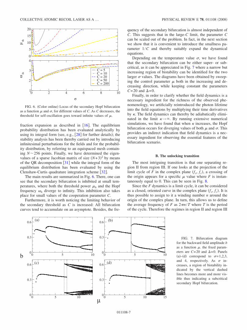
Depending on the temperature value �, we have foundthat the secondary bifurcation can be either super- or sub-critical, as it can be appreciated in Fig. 7 where a narrow butincreasing region of bistability can be identified for the twolarger � values. The diagrams have been obtained by sweep-ing the control parameter � both in the increasing and de-creasing direction, while keeping constant the parametersC=20 and �=0.

Finally, in order to clarify whether the field dynamics is anecessary ingredient for the richness of the observed phe-nomenology, we artificially reintroduced the photon lifetimeinto the field equations by multiplying their time derivativesby �. The field dynamics can thereby be adiabatically elimi-nated in the limit �→�. By running extensive numericalsimulations, we have found that when � increases, the Hopfbifurcation occurs for diverging values of both � and �. Thisprovides an indirect indication that field dynamics is a nec-essary ingredient for observing the essential features of thebifurcation scenario.

B. The unlocking transition

The most intriguing transition is that one separating re-gion II from region III. If one looks at the projection of thelimit cycle of F in the complex plane �fs, fc�, a crossing ofthe origin appears for a specific � value where F is instan-taneously equal to 0. This can be seen in Fig. 8.

Since the F dynamics is a limit cycle, it can be consideredas a closed, oriented curve in the complex plane �fs, fc�. It isthus possible to assign to it a winding number n around theorigin of the complex plane. In turn, this allows us to definethe average frequency of F as 2n /T where T is the periodof the cycle. Therefore the regimes in region II and region III

0

5

10

15

20

µth

C = 5C = 10C = 20C = 50C = 200

0 2 4 6 8 10

σ

1

2

3

4

ωth

FIG. 6. �Color online� Locus of the secondary Hopf bifurcationas a function � and �, for different values of C. As C decreases, thethreshold for self-oscillation goes toward infinite values of �.

0 5 100

0.3

0.6

0 5 100

0.3

0.6

0 5 100

0.3

0.6

0 5 10 150

0.3

0.6

µ

b

(a) (b)

(c) (d)

FIG. 7. Bifurcation diagramfor the backward field amplitude bas a function �. the fixed param-eters are C=20 and �=0. Panels�a�–�d� correspond to �=1,2,3,and 4, respectively. As � in-creases, a region of bistability in-dicated by the vertical dashedlines becomes more and more vis-ible thus indicating a subcriticalsecondary Hopf bifurcation.


011108-7

are characterized by a zero and nonzero average rotation,respectively. One can consider intuitively that the mechanismresponsible for the redshift of the backward field with respectto the input field is at some point responsible for shifting theforward field with respect to the frequency of the backwardone.

A less trivial scenario is found in the �Rc, Rs� plane �seeFig. 9�: only a fraction of the limit cycle remains unchangedwhen passing from below to above the transition point. Theremaining part is made of two complementary halves of acircumference, so that across the transition, the whole limitcycle abruptly encircles the origin, thus signaling the onsetof an order-parameter rotation. In order to further clarifythe transition, let us look at the evolution of the potential tilt

�− �. In Fig. 10 we see that in the vicinity of the singularpoint, where the field amplitude f is close to zero �for thesake of simplicity, we have set the origin of the time axissuch that the minimal distance from the origin occurs at

t=0�, �− � becomes very large, but the sign of this quantityis different above and below the transition, because the ori-gin is encircled only above the transition. In the laboratoryframe, however, the average velocity of the atoms exhibits a

smooth change across the transition; in fact, the discontinu-ous variation of the instantaneous frequency is compensatedby a discontinuous variation of the flux—cf. Eq. �27�. Fi-nally, in Fig. 11 we show the dependency of the average

frequency of both the forward ��, and the backward ��field, as a function of �. There, we can see that both frequen-cies have the same sign and that the redshift of the forwardfield is larger than the one of the backward field. Both fea-tures can be understood by means of the following heuristicargument. We indeed expect that the same mechanism that isresponsible for the redshift of the backward field with respectto the input field should, at some point �when the backwardfield intensity is large enough� be responsible for redshiftingthe forward field with respect to the backward one. This isprecisely what we see.

V. A MINIMAL MODEL

In this section we go back to the general case ��0 andshow how the model can be reduced to a set of five ordinary

0 0.2 0.4 fc

0

0.2

fs

f

φ

FIG. 8. A projection of F in the complex plane, for the criticalvalue �c=2.752, when the forward field unlocks from the inputfield. Parameters are those of Fig. 4 The cycle goes through thepoint F=0.

-0.1 0 0.1 Rc

-0.1

0

0.1

Rs

FIG. 9. �Color online� A projection of two limit cycles just be-low and above the critical point, �c=2.752 where the forward fieldunlocks from the input field. The other parameter values are thoseof Fig. 5. The arrows indicate the direction of the motion: below�above� the transition, in the �un�locked regime, the upper �lower�semicircle is followed.

-0.02 -0.01 0 0.01 0.02t

-2000

-1000

0

φ−β

FIG. 10. �Color online� The behavior of the instantaneous slopeof the potential, just below ��=2.75 dashed line� and above��=2.76 the transition point�. The different amplitude of the twocurves is due to a different distance from the critical point. Param-eters are those of Fig. 4.

2 4 6 8µ0

1

2

3β , φ

2 4 6 8µ0.9

1

1.1

β

FIG. 11. �Color online� Frequency of the forward �dashed line�and backward �solid line� fields, referred to that of the input field, asa function of �. Parameters are the same as in Fig. 4. An enlarge-

ment of the � behavior is plotted in the inset.


011108-8

differential equations that is still able to reproduce the rel-evant phenomenology discussed in the previous section. Westart by assuming that the parameter C is large and introducethe smallness parameter ��C−1/3. As a next step, we per-form the following change of variables, that has been sug-gested by numerical simulations,

t = �� ,

f = �u, b = �v . �29�

Moreover, we express the probability density Q�� , t� as thesum of a homogeneous component and a sinusoidal pertur-bation, namely,

Q��,t� =1

2+ �2S��,�� 30�

and correspondingly define

Rs = �2rs Rc = �2rc. �31�

Accordingly, the equations for the field variables write

du

d�= cos � − �u − vrs,

dvd�

= − �v + urs,

d�

d�= −

sin �

u−

vrc

u− �� ,

d�

d�= −

urc

v− �� . �32�

while the Fokker-Planck equation writes

��S = −��

2uv cos � − ��D� + ��3uv sin ��S + ��

2S ,

�33�

where we have introduced

D� =d�

d�−

d�

d�= rc�u

v−

vu� −

sin �

u�34�

both to keep the notations as compact as possible and toremind that � is not a relevant variable.

So far, no approximation has been introduced, and theabove two sets of equations are equivalent to the initial for-mulation. However, we can recognize the existence of smallterms when � is small. In particular, it is tempting to neglectall terms which are proportional to some �positive� power of�, but this limit is singular. In fact, the resulting model isdissipationless �notice also that all physical parameterswould disappear�. On the one hand, the diffusion term in theFokker-Planck equation disappears as well as the positiondependent force, so that any initial condition for the distri-bution S�� remains invariant in time, which is not physical.On the other hand, the field dynamics is conservative as well�the two loss terms vanish�. Since, finally, as we see below,

there are conserved quantities, it is obvious that any arbi-trarily small dissipation is going to qualitatively modify theasymptotic behavior and we, accordingly, cannot drasticallyset the � terms equal to zero. Nevertheless, we are entitled toneglect the cubic term, which is a less crude hypothesis. Theresulting simplified Fokker-Planck equation can be solvedexactly, assuming that S�� reduces to its first Fourier mode.It is convenient to express the amplitude of such mode di-rectly referring to the two components of the order param-eter,

S�� =1

2��rc + irs�e−i� + c.c.� �35�

We indeed obtain �from now on, we again use a dot to meanthe derivative with respect to the time variable ��

rc = −��

2uv − D�rs − ��rc,

rs = D�rc − ��rs �36�

which complement the first three equations in Eqs. �32�If we now pass to phase and amplitude

rc = r cos �, rs = r sin � �37�

the entire set of equations writes

u = cos � − �u − vr sin � ,

v = − �v + ur sin � ,

� = −rvu

cos � −sin �

u− �� ,

� = D� +��

2

uvr

sin � ,

r = − ��r −��

2uv cos � �38�

while

D� = r cos ��u

v−

vu� −

sin �

u. �39�

Let us now discuss an analogy between our asymptoticlimit and the small gain approximation, or the uniform fieldlimit �UFL�, that are widely used in laser physics. Our ap-proach implicitly assumes a weak action of the fields ontothe atomic sample, i.e., a small dipolar coupling. Thereforethe Bragg grating imprinted onto the atomic density can beconsidered as a small perturbation of a homogeneous sample.On the other hand, one has to assume that the retroaction ofthe atoms onto the cavity is sufficiently strong for the smalldensity modulation to influence the fields, i.e., a large coop-eration parameter C. This approximation can be compared,for instance, with the small gain approximation, where oneassumes that the material gain is simply proportional to itspopulation inversion. This amounts to neglecting nonlinear


011108-9

saturation processes such as power broadening for a two-level atoms or carrier heating for a semiconductor material.Altogether, the asymptotic limit of this section is analogousto the UFL which amounts to considering a weak single passgain within the cavity and, simultaneously, small opticallosses, in such a way that a finite net amplification can even-tually occur.

A. Numerical and theoretical analysis

1. The primary transition with nonzero detuning

Analytic expressions for the steady states of Eqs. �38� arederived in the Appendix. The resulting bifurcation diagramscorresponding to �=0, 2, 3, and −2, respectively, are dis-played in Fig. 12, where, for the sake of clarity, we keepusing the same notations as in the previous section. In par-ticular, we see that for positive and large enough detuningthere exist two branches �besides the trivial one b=0�. Thismeans that the primary bifurcation becomes subcritical, sig-naling the appearance of a bistability region. Still from theanalytic discussion presented in the Appendix, it turns outthat the primary threshold is

�th =1 + �2

C�� − 1� + �� + 1��2 + 4�� . �40�

It is important to notice that this expression holds true alsofor the original model, since in the vicinity of the transition,the behavior of Q�� is by definition dominated by the firstFourier harmonic.

As shown in the Appendix, it is possible to derive ananalytic expression for the saddle-node bifurcation, whichturns out to be

�sn =2

C

�2�� − �3��2 + 4� + �4 + 2�2

��2 + 4� − �. �41�

Notice that this equation makes sense only when both solu-tions of the biquadratic equation �A4� are positive. This can

happen only for � larger than a critical value �c that can bedetermined by setting �sn=�th,

�c =1

��c + 1. �42�

Thus one can conclude that, when � is negative, no bistabil-ity can occur, while it is allowed for a sufficiently large posi-tive detuning.

Finally, in the small temperature limit, the minimumthreshold is achieved for a detuning,

�m = 2�1 − ��

1 + 9� + 8�2 . �43�

Figure 13 shows the spinodal decomposition of the solutionscurve in the �� ,�� plane of both the original and the simpli-fied model �see dashed and solid lines, respectively� for �=1 and C=20. One can see that there is a reasonable agree-ment even though the corresponding � value is not too small��0.36�. The two shaded regions correspond to the mono-and the bistable regimes, respectively. The full circle marksthe tricritical point, where the bistable area appears in theoriginal model.

2. The secondary transition

The almost quantitative agreement between the full andthe simplified model is not solely restricted to steady states.At larger input intensities, the simplified model exhibits ascenario that is very reminiscent of that observed in theoriginal model: a secondary instability is first detected, thatis followed by the unlocking phenomenon and, finally, by asequence of period doubling bifurcations toward a chaoticregime. This indicates that the degrees of freedom that areresponsible for the onset of macroscopic order are the verysame ones leading to the self-pulsating instability. In order toconfirm whether the simplified model is really built on therelevant physical variables, we have investigated whether thelocus of the secondary transition exhibits a similar depen-dence on the control parameters. We proceeded along thesame lines described in Sec. IV A. Our main results are sum-

0 1 2 3 4 50

0.2

0.4

0.6

0.8

1

0 1 2 3 4 50

0.2

0.4

0.6

0.8

1

1 2 3 4 50

0.2

0.4

0.6

0.8

1

1 2 3 4 50

0.2

0.4

0.6

0.8

1

µ

b

(a) (b)

(d)(c)

FIG. 12. Bifurcation diagram of the steady states of Eqs. �38� asa function of �, for C=20 and �=1. Panels �a�–�d� correspond to�=0, 2, 3, and −2, respectively. The dashed lines denote the borderof the bistability regions whenever there is one.

��

��

-4 -2 0 2 4∆

0.1

1

10µ

FIG. 13. �Color online� Spinodal decomposition of the steadystates. Dashed lines refer to the original full model �for �=1 andC=20�; solid lines refer to the simplified model �38�. The twoshaded regions correspond to mono- and bistable regimes in the fullmodel. The circle denotes the tricritical point �c.


011108-10

marized in Fig. 14. There, one can see that the characteristicsof the full model described in Fig. 6 are preserved, like e.g.,inhibition of the transition for small values of either the tem-perature or the cooperation parameter C. By comparing thefull and dashed lines in Fig. 14, one can also notice that analmost quantitative agreement with the full model is obtainedwhenever the value of �th is not too large. Otherwise, theapproximation, that consists in truncating the Fourier expan-sion of the probability distribution after the first mode,breaks. The overall quantitative agreement is reasonablygood for values down to C=50, regardless of the value of thetemperature �.

B. The C\� limit

Since the highest degree of dynamical complexityamounts to a sequence of period-doubling bifurcations, onemight wonder whether it is possible to further reduce thedimensionality of the model from five to three degrees offreedom. In order to clarify this question we now considerthe limit �→0 and, for the sake of simplicity, we restrict theanalysis to the resonant case �=0. It is, unfortunately, nec-essary to perform a further change of variables; namely weintroduce

uc = u cos �; us = u sin � �44�

and

vc = v cos�� − ��; vs = v sin�� − �� . �45�

The resulting equations read

r = − ��r −��

2�vcuc − vsus� ,

uc = 1 − rvs − �uc,

us = − rvc − �us,

vc = rus − �vc −��

2

vs

r�vsuc + vcus� ,

vs = ruc − �vs +��

2

vc

r�vsuc + vcus� . �46�

The great advantage of this representation is that in the �→0 limit, it factorizes into three independent and partiallydegenerate blocks,

r = 0,

uc = − r2uc,

us = − r2us �47�

characterized by three constants of motion,

C1 = r ,

C22 = �vs − 1/r�2 + uc

2,

C32 = vc

2 + us2. �48�

Accordingly, a general solution writes as

vs =1

C1+ C2 sin�C1t + �1� ,

uc = C2 cos�C1t + �1� ,

vc = C3 sin�C1t + �2� ,

us = C3 cos�C1t + �2� �49�

from which it is clear that two other constants enter thegame, namely the phases �1, and �2. However, one phasecan be removed by shifting the origin of the time axis,namely by introducing the phase difference �=�2−�1. Thuswe see that altogether, it should be possible at least to re-move one out of the five variables. However, rather thanpursuing this goal, we prefer to limit our discussion to theproblem of determining the value of all the relevant con-stants. In order to do that, it is necessary to reintroduce afinite smallness parameter � and thereby determine the timederivative of the various “constants.” By denoting with aprime the derivative with respect to ��, we find

C1� = − �C1 −�

2C2C3 sin � ,

C2� = − C2 +�C3

16C13 ��C2

2 − C32�C1

2 − 4�sin � ,

C3� = − C3 −�C2

16C13 ��C2

2 − C32�C1

2 + 4�sin � ,

0

5

10

15

20

µth

C = 10C = 50C = 200

0 2 4 6 8 10

σ

2

3

4

ωth

FIG. 14. �Color online� Locus of the secondary instability as afunction � and �, for different values of C. Predictions of the sim-plified model, Eqs. �38�, with dashed lines, are compared with thoseof the exact model, Eqs. �10�–�14�, with solid lines. Parameters arethose of Fig. 6.


011108-11

�� = −�

16C13 ��C2

2 + C32�C1

2 + 4��C3

C2+

C2

C3�cos � . �50�

These equations admit a pair of symmetric fixed pointswhich correspond to a periodic dynamics in the original vari-ables,

� = �

2, C1 = � ��

4�1/3

, C22 = C3

2 =�

2� 4

��2/3

.

�51�

Therefore the most robust dynamics which persists in theC→� limit is the periodic one, arising after the Hopf bifur-cation.

VI. CONCLUSION

By recasting a known CARL model as a self-consistentequation for the probability distribution, we have been ableto discuss analogies and differences with the Kuramotomodel for synchronization in ensemble of globally coupledrotators. In fact, although the primary transition, giving riseto the spontaneous formation of a density grating, resemblesthe onset of a macroscopic synchronized state in the Kura-moto model, there are important differences. In particular,the global coupling affects the frequency of the oscillators�here, the velocity of the atoms�, determining the tilting ofthe effective washboard potential. Another difference con-cerns the existence, in the CARL context, of an “absolute”reference frame, the only one where the equations are timeindependent. As a result of these differences, we find asubtlety in the macroscopic behavior: the average velocity ofthe grating does not coincide with the average velocity of thesingle atoms. Such a feature is reminiscent of the collectivebehavior discussed in �21�, where it is shown that nonlinearall-to-all interactions may lead to the onset of a peculiar pe-riodic macroscopic phase. That phase is �in the absence ofexternal noise� both characterized by a microscopic quasip-eriodic motion and an average frequency of the single oscil-lators that differs from the period of the macroscopic motion.However, the correspondence between this behavior and thecollective atomic motion arising beyond the primary thresh-old is perhaps incomplete, since in the CARL context, theperiodic global dynamics reduces to a fixed point in the “ab-solute” reference frame. A more promising candidate to es-tablish a full analogy is the periodic motion arising beyondthe unlocking transition, although the presence of micro-scopic stochastic fluctuations makes it difficult to formulate aconvincing final statement. In fact, on the one hand, quasip-eriodicity can be recognized as such only in deterministicsystems, and, on the other hand, we are aware of at leastanother mechanism leading to periodic oscillations in glo-bally coupled noisy rotators �see, e.g., �4��. Unfortunately, inthe context of cold atoms, we cannot consider directly thezero-noise limit, as it corresponds to a qualitatively differentregime, namely full synchronization. Therefore until an ob-jective criterion of distinguishing possibly different classesof periodic collective motions is introduced, the problem willremain open.

Finally, we wish to recall that the rich phenomenologyextensively discussed in this paper is experimentally acces-sible, since we have everywhere �with the only exception ofthe zero-temperature limit� considered parameter values thatare compatible with the experiment discussed in �1�. Theonly important constraint comes from the need to stabilizeand control a priori of the frequency of the input field, with-out the help of any feedback coming from the output of thecavity itself as done in Ref. �1�.

ACKNOWLEDGMENTS

We wish to thank G. L. Lippi for useful discussions. J.J.acknowledges support from the program Juan de la Cierva,Ministerio de Educación y Ciencia. A.P. acknowledges finan-cial support from the Max Planck Institute for Complex Sys-tems �Dresden� where this work was initiated as well assupport of the PRIN on “Dynamics and thermodynamics ofsystems with long-range interactions.”

APPENDIX

In this appendix we determine the steady states of Eqs.�38�, by setting all the derivatives equal to zero. From thesecond and the last of them, one obtains

sin � =�vur

,

cos � = −2�r

�uv. �A1�

By now subtracting the fourth from the third equation in theset �38� and thereby eliminating sin � and cos � with the helpof Eq. �A1�, we obtain a biquadratic equation in s=v /r. Suchan equation has always one and only one positive, and thusphysically acceptable, solution,

��

2s2 = −

�

2+

�

2��2 + 4� . �A2�

By now squaring and summing the two expressions for sin �and cos � in Eq. �A1� we find that the intensity of the for-ward field is

u2 = �2s2 +4�2

�2

1

s2 . �A3�

The last step consists in solving the first and third equa-tion in Eq. �38� for cos � and sin �, respectively, squaringand summing. As a result, we obtain a biquadratic equationfor r,

c4r4 + c2r2 + c0 = 0, �A4�

where

c4 = �2s4 +4�2

�2 ,

c2 = 2u2��s2 −2��

�� ,


011108-12

c0 = u2��2u2�1 + �2� − 1� .

The bifurcation point of the homogeneous state r=0 is foundby setting c0=0. With the help of Eqs. �A2� and �A3�, thiscondition transforms into Eq. �40�, displayed in Sec. V.

Moreover, the above biquadratic equation may have twodistinct nontrivial solutions. The critical point where a pair ofsolutions is created �the saddle-node bifurcation� can be de-termined by imposing

c22 − 4c4c0 = 0. �A5�

With the help of Eqs. �A2� and �A3�, this condition trans-forms into Eq. �41�. Notice that this condition makes senseonly when the two resulting solutions are both larger thanzero, i.e., when c2 /c4�0. Finally, from the way the solutionshave been derived, one can observe a curious property: thetwo branches are characterized by the same amplitude of theforward field.

�1� D. Kruse, C. von Cube, C. Zimmermann, and Ph. W.Courteille, Phys. Rev. Lett. 91, 183601 �2003�.

�2� R. Bonifacio and L. De Salvo, Nucl. Instrum. Methods Phys.Res. A 341, 360 �1994�; R. Bonifacio, L. De Salvo, L. M.Narducci, and E. J. D’Angelo, Phys. Rev. A 50, 1716 �1994�.

�3� K. Kometani and H. Shimizu, J. Stat. Phys. 13, 473 �1975�; R.C. Desai and R. Zwanzig, ibid. 19, 1 �1978�.

�4� L. L. Bonilla, J. M. Casado, and M. Morillo, J. Stat. Phys. 48,571 �1987�.

�5� A. S. Pikovsky, M. G. Rosenblum, and J. Kurths, Europhys.Lett. 34, 165 �1996�.

�6� Y. Kuramoto, Chemical Oscillations, Waves and Turbulence�Springer, Berlin, 1984�.

�7� L. F. Abbott and C. van Vreeswijk, Phys. Rev. E 48, 1483�1993�.

�8� A. Zumdieck, M. Timme, T. Geisel, and F. Wolf, Phys. Rev.Lett. 93, 244103 �2004�.

�9� C. Cohen-Tannoudji, J. Dupont-Roc, and G. Grynberg, Atom-Photon Interactions: Basic Processes and Applications �Wiley,New York, 1992�.

�10� L. R. Elias, W. M. Fairbank, J. M. J. Madey, H. A. Schwett-man, and T. I. Smith, Phys. Rev. Lett. 36, 717 �1976�.

�11� G. L. Lippi, G. P. Barozzi, S. Barbay, and J. R. Tredicce, Phys.Rev. Lett. 76, 2452 �1996�.

�12� P. R. Hemmer, N. P. Bigelow, D. P. Katz, M. S. Shahriar, L.DeSalvo, and R. Bonifacio, Phys. Rev. Lett. 77, 1468 �1996�.

�13� W. J. Brown, J. R. Gardner, D. J. Gauthier, and R. Vilaseca,Phys. Rev. A 55, R1601 �1997�.

�14� M. Perrin, G. L. Lippi, and A. Politi, Phys. Rev. Lett. 86, 4520�2001�.

�15� J. Javaloyes, G. L. Lippi, and A. Politi, Phys. Rev. A 68,

033405 �2003�.�16� J. Javaloyes, M. Perrin, G. L. Lippi, and A. Politi, Phys. Rev.

A 70, 023405 �2004�.�17� G. R. M. Robb, N. Piovella, A. Ferraro, R. Bonifacio, Ph. W.

Courteille, and C. Zimmermann, Phys. Rev. A 69, 041403�R��2004�.

�18� C. von Cube, S. Slama, D. Kruse, C. Zimmermann, Ph. W.Courteille, G. R. M. Robb, N. Piovella, and R. Bonifacio,Phys. Rev. Lett. 93, 083601 �2004�.

�19� C. van Vreeswijk, Phys. Rev. E 54, 5522 �1996�.�20� P. K. Mohanty and A. Politi, J. Phys. A 39, L415 �2006�.�21� M. Rosenblum and A. Pikovsky, Phys. Rev. Lett. 98, 064101

�2007�.�22� R. Bonifacio, G. R. M. Robb, and B. W. J. McNeil, Phys. Rev.

A 56, 912 �1997�.�23� M. Perrin, Z. Ye, and L. M. Narducci, Phys. Rev. A 66,

043809 �2002�.�24� Z. Ye and L. M. Narducci, Phys. Rev. A 63, 043815 �2001�.�25� P. L. Bhatnagar, E. P. Gross, and M. Krook, Phys. Rev. 94, 511

�1954�.�26� R. Bonifacio and P. Verkerk, Opt. Commun. 124, 469 �1996�.�27� C. N. Cohen-Tannoudji, Rev. Mod. Phys. 70, 707 �1998�.�28� H. Risken, The Fokker-Planck Equation �Springer, Berlin,

1984�.�29� R. Adler, Proc. IEEE 61, 1380 �1973�; reprinted from Proc.

IRE 34 �6�, 351 �1946�.�30� S. Nichols and K. Wiesenfeld, Phys. Rev. A 45, 8430 �1992�.�31� D. E. Stewart, Meschach Linear Algebra Library in C,

http://www.math.uiowa.edu/~dstewart/meschach/�32� T. Ooura and A. Clenshaw-Curtis, Quadrature package in C,

http://www.kurims.kyoto-u.ac.jp/~ooura/


011108-13

collective atomic recoil laser as a synchronization transition · collective atomic recoil laser as...

Documents