college algebra - lamar universitytutorial.math.lamar.edu/dodownload.aspx?u=pdf/alg/... · college...

COLLEGE ALGEBRA Systems of Equations

Paul Dawkins

College Algebra

© 2007 Paul Dawkins i http://tutorial.math.lamar.edu/terms.aspx

Table of Contents

Preface ............................................................................................................................................ ii Systems of Equations ..................................................................................................................... 3

Introduction ................................................................................................................................................ 3 Linear Systems with Two Variables .......................................................................................................... 4 Linear Systems with Three Variables .......................................................................................................12 Augmented Matrices .................................................................................................................................16 More on the Augmented Matrix ................................................................................................................25 Non-Linear Systems ..................................................................................................................................31

College Algebra

© 2007 Paul Dawkins ii http://tutorial.math.lamar.edu/terms.aspx

Preface Here are my online notes for my Algebra course that I teach here at Lamar University, although I have to admit that it’s been years since I last taught this course. At this point in my career I mostly teach Calculus and Differential Equations. Despite the fact that these are my “class notes”, they should be accessible to anyone wanting to learn Algebra or needing a refresher for algebra. I’ve tried to make the notes as self contained as possible and do not reference any book. However, they do assume that you’ve had some exposure to the basics of algebra at some point prior to this. While there is some review of exponents, factoring and graphing it is assumed that not a lot of review will be needed to remind you how these topics work. Here are a couple of warnings to my students who may be here to get a copy of what happened on a day that you missed.

1. Because I wanted to make this a fairly complete set of notes for anyone wanting to learn algebra I have included some material that I do not usually have time to cover in class and because this changes from semester to semester it is not noted here. You will need to find one of your fellow class mates to see if there is something in these notes that wasn’t covered in class.

2. Because I want these notes to provide some more examples for you to read through, I don’t always work the same problems in class as those given in the notes. Likewise, even if I do work some of the problems in here I may work fewer problems in class than are presented here.

3. Sometimes questions in class will lead down paths that are not covered here. I try to anticipate as many of the questions as possible in writing these up, but the reality is that I can’t anticipate all the questions. Sometimes a very good question gets asked in class that leads to insights that I’ve not included here. You should always talk to someone who was in class on the day you missed and compare these notes to their notes and see what the differences are.

4. This is somewhat related to the previous three items, but is important enough to merit its own item. THESE NOTES ARE NOT A SUBSTITUTE FOR ATTENDING CLASS!! Using these notes as a substitute for class is liable to get you in trouble. As already noted not everything in these notes is covered in class and often material or insights not in these notes is covered in class.

College Algebra

© 2007 Paul Dawkins 3 http://tutorial.math.lamar.edu/terms.aspx

Systems of Equations

Introduction This is a fairly short chapter devoted to solving systems of equations. A system of equations is a set of equations each containing one or more variable. We will focus exclusively on systems of two equations with two unknowns and three equations with three unknowns although the methods looked at here can be easily extended to more equations. Also, with the exception of the last section we will be dealing only with systems of linear equations. Here is a list of the topics in this section. Linear Systems with Two Variables – In this section we will use systems of two equations and two variables to introduce two of the main methods for solving systems of equations. Linear Systems with Three Variables – Here we will work a quick example to show how to use the methods to solve systems of three equations with three variables. Augmented Matrices – We will look at the third main method for solving systems in this section. We will look at systems of two equations and systems of three equations. More on the Augmented Matrix – In this section we will take a look at some special cases to the solutions to systems and how to identify them using the augmented matrix method. Nonlinear Systems – We will take a quick look at solving nonlinear systems of equations in this section.

College Algebra


Linear Systems with Two Variables A linear system of two equations with two variables is any system that can be written in the form.

ax by pcx dy q

+ =+ =

where any of the constants can be zero with the exception that each equation must have at least one variable in it. Also, the system is called linear if the variables are only to the first power, are only in the numerator and there are no products of variables in any of the equations. Here is an example of a system with numbers.

3 7

2 3 1x y

x y− =+ =

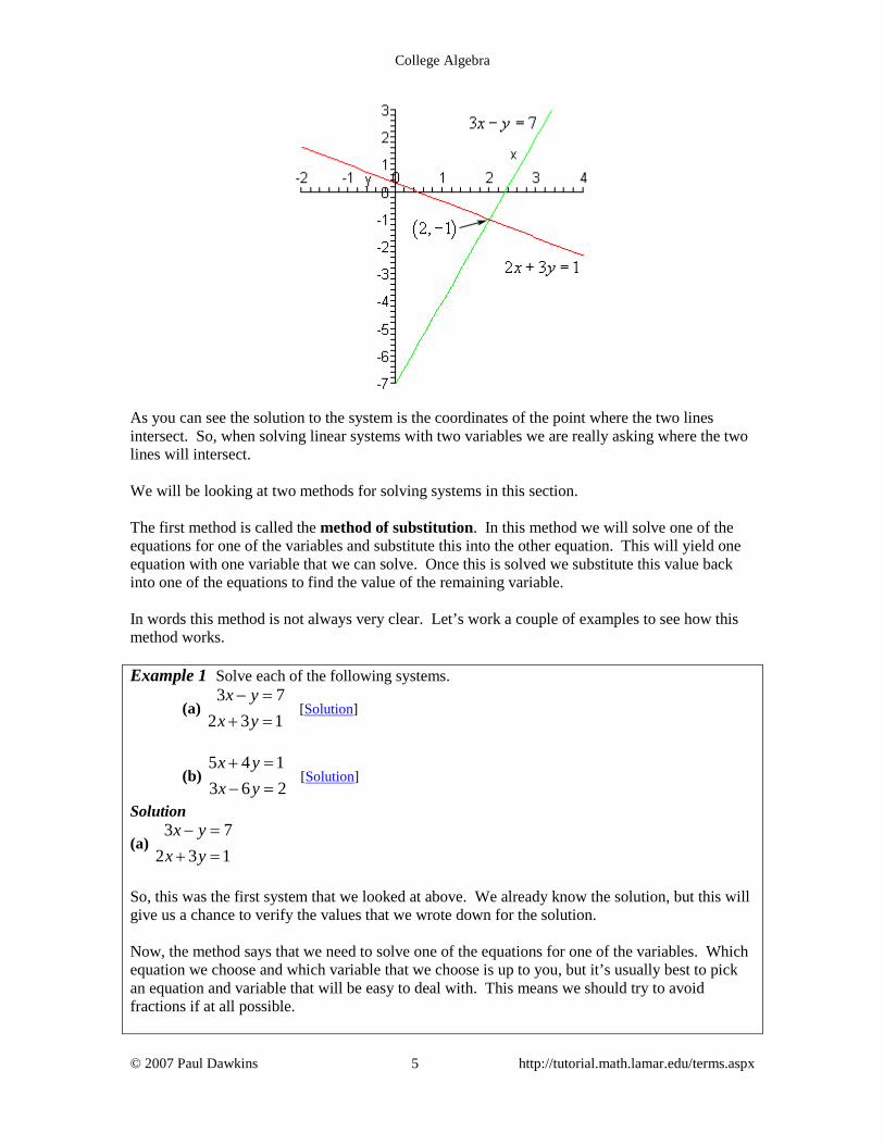
Before we discuss how to solve systems we should first talk about just what a solution to a system of equations is. A solution to a system of equations is a value of x and a value of y that, when substituted into the equations, satisfies both equations at the same time. For the example above 2x = and 1y = − is a solution to the system. This is easy enough to check.

( ) ( )

( ) ( )3 2 1 7

2 2 3 1 1

− − =

+ − =

So, sure enough that pair of numbers is a solution to the system. Do not worry about how we got these values. This will be the very first system that we solve when we get into examples. Note that it is important that the pair of numbers satisfy both equations. For instance 1x = and

4y = − will satisfy the first equation, but not the second and so isn’t a solution to the system. Likewise, 1x = − and 1y = will satisfy the second equation but not the first and so can’t be a solution to the system. Now, just what does a solution to a system of two equations represent? Well if you think about it both of the equations in the system are lines. So, let’s graph them and see what we get.

College Algebra


As you can see the solution to the system is the coordinates of the point where the two lines intersect. So, when solving linear systems with two variables we are really asking where the two lines will intersect. We will be looking at two methods for solving systems in this section. The first method is called the method of substitution. In this method we will solve one of the equations for one of the variables and substitute this into the other equation. This will yield one equation with one variable that we can solve. Once this is solved we substitute this value back into one of the equations to find the value of the remaining variable. In words this method is not always very clear. Let’s work a couple of examples to see how this method works. Example 1 Solve each of the following systems.

(a) 3 7

2 3 1x y

x y− =+ =

[Solution]

(b) 5 4 13 6 2x yx y+ =− =

[Solution]

Solution

(a) 3 7

2 3 1x y

x y− =+ =

So, this was the first system that we looked at above. We already know the solution, but this will give us a chance to verify the values that we wrote down for the solution. Now, the method says that we need to solve one of the equations for one of the variables. Which equation we choose and which variable that we choose is up to you, but it’s usually best to pick an equation and variable that will be easy to deal with. This means we should try to avoid fractions if at all possible.

College Algebra


In this case it looks like it will be really easy to solve the first equation for y so let’s do that. 3 7x y− = Now, substitute this into the second equation. ( )2 3 3 7 1x x+ − = This is an equation in x that we can solve so let’s do that.

2 9 21 1

11 222

x xxx

+ − ===

So, there is the x portion of the solution. Finally, do NOT forget to go back and find the y portion of the solution. This is one of the more common mistakes students make in solving systems. To so this we can either plug the x value into one of the original equations and solve for y or we can just plug it into our substitution that we found in the first step. That will be easier so let’s do that. ( )3 7 3 2 7 1y x= − = − = − So, the solution is 2x = and 1y = − as we noted above.

[Return to Problems]

(b) 5 4 13 6 2x yx y+ =− =

With this system we aren’t going to be able to completely avoid fractions. However, it looks like if we solve the second equation for x we can minimize them. Here is that work.

3 6 2

223

x y

x y

= +

= +

Now, substitute this into the first equation and solve the resulting equation for y.

25 2 4 131010 4 13

10 714 13 37 13 14

16

y y

y y

y

y

y

+ + =

+ + =

= − = −

= −

= −

College Algebra


Finally, substitute this into the original substitution to find x.

1 2 1 2 126 3 3 3 3

x = − + = − + =

So, the solution to this system is 13

x = and 16

y = − .

[Return to Problems] As with single equations we could always go back and check this solution by plugging it into both equations and making sure that it does satisfy both equations. Note as well that we really would need to plug into both equations. It is quite possible that a mistake could result in a pair of numbers that would satisfy one of the equations but not the other one. Let’s now move into the next method for solving systems of equations. As we saw in the last part of the previous example the method of substitution will often force us to deal with fractions, which adds to the likelihood of mistakes. This second method will not have this problem. Well, that’s not completely true. If fractions are going to show up they will only show up in the final step and they will only show up if the solution contains fractions. This second method is called the method of elimination. In this method we multiply one or both of the equations by appropriate numbers (i.e. multiply every term in the equation by the number) so that one of the variables will have the same coefficient with opposite signs. Then next step is to add the two equations together. Because one of the variables had the same coefficient with opposite signs it will be eliminated when we add the two equations. The result will be a single equation that we can solve for one of the variables. Once this is done substitute this answer back into one of the original equations. As with the first method it’s much easier to see what’s going on here with a couple of examples. Example 2 Solve each of the following systems of equations.

(a) 5 4 13 6 2x yx y+ =− =

[Solution]

(b) 2 4 106 3 6x yx y+ = −+ =

[Solution]

Solution

(a) 5 4 13 6 2x yx y+ =− =

This is the system in the previous set of examples that made us work with fractions. Working it here will show the differences between the two methods and it will also show that either method can be used to get the solution to a system. So, we need to multiply one or both equations by constants so that one of the variables has the same coefficient with opposite signs. So, since the y terms already have opposite signs let’s work with these terms. It looks like if we multiply the first equation by 3 and the second equation by 2

College Algebra


the y terms will have coefficients of 12 and -12 which is what we need for this method. Here is the work for this step.

5 4 1 3 15 12 3

3 6 2 2 6 12 4

21 7

x y x y

x y x y

x

+ = × + =

− = × − =

=

So, as the description of the method promised we have an equation that can be solved for x.

Doing this gives, 13

x = which is exactly what we found in the previous example. Notice

however, that the only fraction that we had to deal with to this point is the answer itself which is different from the method of substitution. Now, again don’t forget to find y. In this case it will be a little more work than the method of substitution. To find y we need to substitute the value of x into either of the original equations and solve for y. Since x is a fraction let’s notice that, in this case, if we plug this value into the second equation we will lose the fractions at least temporarily. Note that often this won’t happen and we’ll be forced to deal with fractions whether we want to or not.

13 6 23

1 6 26 1

16

y

yy

y

− =

− =− =

= −

Again, this is the same value we found in the previous example.


(b) 2 4 106 3 6x yx y+ = −+ =

In this part all the variables are positive so we’re going to have to force an opposite sign by multiplying by a negative number somewhere. Let’s also notice that in this case if we just multiply the first equation by -3 then the coefficients of the x will be -6 and 6. Sometimes we only need to multiply one of the equations and can leave the other one alone. Here is this work for this part.

2 4 10 3 6 12 30

6 3 6 same 6 3 6

9 364

x y x y

x y x y

yy

+ = − × − − − =

+ = + =

− == −

Finally, plug this into either of the equations and solve for x. We will use the first equation this

College Algebra


time.

( )2 4 4 102 16 10

2 63

xx

xx

+ − = −

− = −==

So, the solution to this system is 3x = and 4y = − .

[Return to Problems] There is a third method that we’ll be looking at to solve systems of two equations, but it’s a little more complicated and is probably more useful for systems with at least three equations so we’ll look at it in a later section. Before leaving this section we should address a couple of special case in solving systems. Example 3 Solve the following systems of equations.

6

2 2 1x y

x y− =

− + =

Solution We can use either method here, but it looks like substitution would probably be slightly easier. We’ll solve the first equation for x and substitute that into the second equation.

( )

6

2 6 2 112 2 2 1

12 1 ??

x y

y yy y

= +

− + + =

− − + =− =

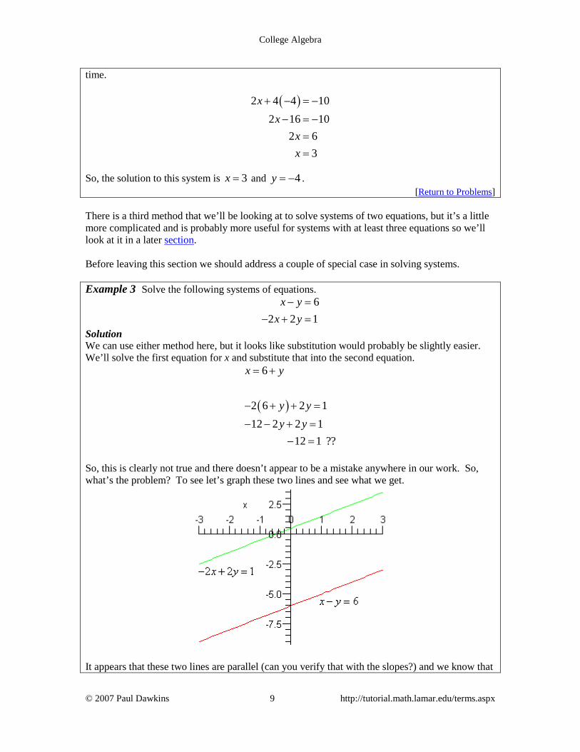
So, this is clearly not true and there doesn’t appear to be a mistake anywhere in our work. So, what’s the problem? To see let’s graph these two lines and see what we get.

It appears that these two lines are parallel (can you verify that with the slopes?) and we know that

College Algebra


two parallel lines with different y-intercepts (that’s important) will never cross. As we saw in the opening discussion of this section solutions represent the point where two lines intersect. If two lines don’t intersect we can’t have a solution. So, when we get this kind of nonsensical answer from our work we have two parallel lines and there is no solution to this system of equations. The system in the previous example is called inconsistent. Note as well that if we’d used elimination on this system we would have ended up with a similar nonsensical answer. Example 4 Solve the following system of equations.

2 5 1

10 25 5x y

x y+ = −

− − =

Solution In this example it looks like elimination would be the easiest method.

2 5 1 5 10 25 5

10 25 5 same 10 25 5

0 0

x y x y

x y x y

+ = − × + = −

− − = − − =

=

On first glance this might appear to be the same problem as the previous example. However, in that case we ended up with an equality that simply wasn’t true. In this case we have 0=0 and that is a true equality and so in that sense there is nothing wrong with this. However, this is clearly not what we were expecting for an answer here and so we need to determine just what is going on. We’ll leave it to you to verify this, but if you find the slope and y-intercepts for these two lines you will find that both lines have exactly the same slope and both lines have exactly the same y-intercept. So, what does this mean for us? Well if two lines have the same slope and the same y-intercept then the graphs of the two lines are the same graph. In other words, the graphs of these two lines are the same graph. In these cases any set of points that satisfies one of the equations will also satisfy the other equation. Also, recall that the graph of an equation is nothing more than the set of all points that satisfies the equation. In other words, there is an infinite set of points that will satisfy this set of equations. In these cases we do want to write down something for a solution. So what we’ll do is solve one of the equations for one of the variables (it doesn’t matter which you choose). We’ll solve the first for y.

2 5 1

5 2 12 15 5

x yy x

y x

+ = −= − −

= − −

Then, given any x we can find a y and these two numbers will form a solution to the system of equations. We usually denote this by writing the solution as follows,

College Algebra


where is any real number2 15 5

x tt

y t

=

= − −

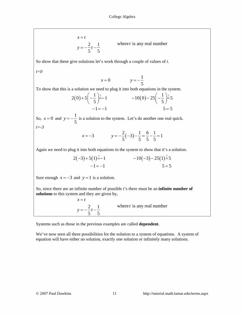
So show that these give solutions let’s work through a couple of values of t. t=0

105

x y= = −

To show that this is a solution we need to plug it into both equations in the system.

( ) ( )? ?1 12 0 5 1 10 0 25 5

5 51 1 5 5

+ − =− − − − = − = − =

So, 0x = and 15

y = − is a solution to the system. Let’s do another one real quick.

t=-3

( )2 1 6 13 3 15 5 5 5

x y= − = − − − = − =

Again we need to plug it into both equations in the system to show that it’s a solution.

( ) ( ) ( ) ( )? ?2 3 5 1 1 10 3 25 1 51 1 5 5

− + =− − − − =

− = − =

Sure enough 3x = − and 1y = is a solution. So, since there are an infinite number of possible t’s there must be an infinite number of solutions to this system and they are given by,

where is any real number2 15 5

x tt

y t

=

= − −

Systems such as those in the previous examples are called dependent. We’ve now seen all three possibilities for the solution to a system of equations. A system of equation will have either no solution, exactly one solution or infinitely many solutions.

College Algebra


Linear Systems with Three Variables This is going to be a fairly short section in the sense that it’s really only going to consist of a couple of examples to illustrate how to take the methods from the previous section and use them to solve a linear system with three equations and three variables. So, let’s get started with an example. Example 1 Solve the following system of equations.

2 3 7

2 43 2 2 10

x y zx y z

x y z

− + =+ + =

− + − = −

Solution We are going to try and find values of x, y, and a z that will satisfy all three equations at the same time. We are going to use elimination to eliminate one of the variables from one of the equations and two of the variables from another of the equations. The reason for doing this will be apparent once we’ve actually done it. The elimination method in this case will work a little differently than with two equations. As with two equations we will multiply as many equations as we need to so that if we start adding pairs of equations we can eliminate one of the variables. In this case it looks like if we multiply the second equation by 2 it will be fairly simple to eliminate the y term from the second and third equation by adding the first equation to both of them. So, let’s first multiply the second equation by two.

2 3 7 same 2 3 7

2 4 2 4 2 2 8

3 2 2 10 same 3 2 2 10

x y z x y zx y z x y z

x y z x y z

− + = − + =+ + = × + + =

− + − = − − + − = −

Now, with this new system we will replace the second equation with the sum of the first and second equations and we will replace the third equation with the sum of the first and third equations. Here is the resulting system of equations.

2 3 7

5 5 152 3

x y zx zx z

− + =+ =

− + = −

So, we’ve eliminated one of the variables from two of the equations. We now need to eliminate either x or z from either the second or third equations. Again, we will use elimination to do this. In this case we will multiply the third equation by -5 since this will allow us to eliminate z from this equation by adding the second onto is.

College Algebra


2 3 7 same 2 3 7

5 5 15 same 5 5 152 3 5 10 5 15

x y z x y zx z x zx z x z

− + = − + =+ = + =

− + = − × − − =

Now, replace the third equation with the sum of the second and third equation.

2 3 7

5 5 1515 30

x y zx zx

− + =+ =

=

Now, at this point notice that the third equation can be quickly solved to find that 2x = . Once we know this we can plug this into the second equation and that will give us an equation that we can solve for z as follows.

( )5 2 5 1510 5 15

5 51

zzzz

+ =

+ ===

Finally, we can substitute both x and z into the first equation which we can use to solve for y. Here is that work.

( )2 2 3 1 72 5 7

2 21

yy

yy

− + =

− + =− =

= −

So, the solution to this system is 2x = , 1y = − and 1z = . That was a fair amount of work and in this case there was even less work than normal because in each case we only had to multiply a single equation to allow us to eliminate variables. In the next section we’ll be looking at a third method for solving systems that is basically a shorthand method for what we did in the previous example. The work using that method will be messy as well, but it will be slightly easier to do once you get the hang of it. In the previous example all we did was use the method of elimination until we could start solving for the variables and then just back substitute known values of variables into previous equations to find the remaining unknown variables. Not every linear system with three equations and three variables uses the elimination method exclusively so let’s take a look at another example where the substitution method is used, at least partially. Example 2 Solve the following system of equations.

College Algebra


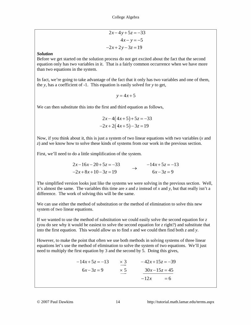
2 4 5 33

4 52 2 3 19

x y zx y

x y z

− + = −− = −

− + − =

Solution Before we get started on the solution process do not get excited about the fact that the second equation only has two variables in it. That is a fairly common occurrence when we have more than two equations in the system. In fact, we’re going to take advantage of the fact that it only has two variables and one of them, the y, has a coefficient of -1. This equation is easily solved for y to get, 4 5y x= + We can then substitute this into the first and third equation as follows,

( )( )

2 4 4 5 5 332 2 4 5 3 19

x x zx x z− + + = −

− + + − =

Now, if you think about it, this is just a system of two linear equations with two variables (x and z) and we know how to solve these kinds of systems from our work in the previous section. First, we’ll need to do a little simplification of the system.

2 16 20 5 33 14 5 13

2 8 10 3 19 6 3 9x x z x z

x x z x z− − + = − − + = −

→− + + − = − =

The simplified version looks just like the systems we were solving in the previous section. Well, it’s almost the same. The variables this time are x and z instead of x and y, but that really isn’t a difference. The work of solving this will be the same. We can use either the method of substitution or the method of elimination to solve this new system of two linear equations. If we wanted to use the method of substitution we could easily solve the second equation for z (you do see why it would be easiest to solve the second equation for z right?) and substitute that into the first equation. This would allow us to find x and we could then find both z and y. However, to make the point that often we use both methods in solving systems of three linear equations let’s use the method of elimination to solve the system of two equations. We’ll just need to multiply the first equation by 3 and the second by 5. Doing this gives,

14 5 13 3 42 15 39

6 3 9 5 30 15 45

12 6

x z x z

x z x z

x

− + = − × − + = −

− = × − =

− =

College Algebra


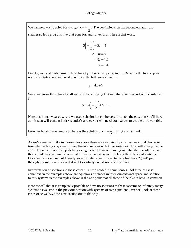
We can now easily solve for x to get 12

x = − . The coefficients on the second equation are

smaller so let’s plug this into that equation and solve for z. Here is that work.

16 3 92

3 3 93 12

4

z

zzz

− − =

− − =− =

= −

Finally, we need to determine the value of y. This is very easy to do. Recall in the first step we used substitution and in that step we used the following equation. 4 5y x= + Since we know the value of x all we need to do is plug that into this equation and get the value of y.

14 5 32

y = − + =

Note that in many cases where we used substitution on the very first step the equation you’ll have at this step will contain both x’s and z’s and so you will need both values to get the third variable.

Okay, to finish this example up here is the solution : 12

x = − , 3y = and 4z = − .

As we’ve seen with the two examples above there are a variety of paths that we could choose to take when solving a system of three linear equations with three variables. That will always be the case. There is no one true path for solving these. However, having said that there is often a path that will allow you to avoid some of the mess that can arise in solving these types of systems. Once you work enough of these types of problems you’ll start to get a feel for a “good” path through the solution process that will (hopefully) avoid some of the mess. Interpretation of solutions in these cases is a little harder in some senses. All three of these equations in the examples above are equations of planes in three dimensional space and solution to this systems in the examples above is the one point that all three of the planes have in common. Note as well that it is completely possible to have no solutions to these systems or infinitely many systems as we saw in the previous section with systems of two equations. We will look at these cases once we have the next section out of the way.

College Algebra


Augmented Matrices In this section we need to take a look at the third method for solving systems of equations. For systems of two equations it is probably a little more complicated than the methods we looked at in the first section. However, for systems with more equations it is probably easier than using the method we saw in the previous section. Before we get into the method we first need to get some definitions out of the way. An augmented matrix for a system of equations is a matrix of numbers in which each row represents the constants from one equation (both the coefficients and the constant on the other side of the equal sign) and each column represents all the coefficients for a single variable. Let’s take a look at an example. Here is the system of equations that we looked at in the previous section.

2 3 7

2 43 2 2 10

x y zx y z

x y z

− + =+ + =

− + − = −

Here is the augmented matrix for this system.

1 2 3 72 1 1 43 2 2 10

− − − −

The first row consists of all the constants from the first equation with the coefficient of the x in the first column, the coefficient of the y in the second column, the coefficient of the z in the third column and the constant in the final column. The second row is the constants from the second equation with the same placement and likewise for the third row. The dashed line represents where the equal sign was in the original system of equations and is not always included. This is mostly dependent on the instructor and/or textbook being used. Next we need to discuss elementary row operations. There are three of them and we will give both the notation used for each one as well as an example using the augmented matrix given above.

1. Interchange Two Rows. With this operation we will interchange all the entries in row i and row j. The notation we’ll use here is i jR R↔ . Here is an example.

1 3

1 2 3 7 3 2 2 102 1 1 4 2 1 1 43 2 2 10 1 2 3 7

R R− − − −

↔ → − − − −

So, we do exactly what the operation says. Every entry in the third row moves up to the first row and every entry in the first row moves down to the third row. Make sure that you move all the entries. One of the more common mistakes is to forget to move one or more entries.

College Algebra


2. Multiply a Row by a Constant. In this operation we will multiply row i by a constant c and the notation will use here is icR . Note that we can also divide a row by a constant

using the notation 1

iRc

. Here is an example.

3

1 2 3 7 1 2 3 74

2 1 1 4 2 1 1 43 2 2 10 12 8 8 40

R− −

− → − − − −

So, when we say we will multiply a row by a constant this really means that we will multiply every entry in that row by the constant. Watch out for signs in this operation and make sure that you multiply every entry.

3. Add a Multiple of a Row to Another Row. In this operation we will replace row i with

the sum of row i and a constant, c, times row j. The notation we’ll use for this operation is i j iR cR R+ → . To perform this operation we will take an entry from row i and add to it c times the corresponding entry from row j and put the result back into row i. Here is an example of this operation.

3 1 3

1 2 3 7 1 2 3 74

2 1 1 4 2 1 1 43 2 2 10 7 10 14 38

R R R− −

− → → − − − − − −

Let’s go through the individual computation to make sure you followed this.

( )( )( )( )

3 4 1 7

2 4 2 10

2 4 3 14

10 4 7 38

− − = −

− − =

− − = −

− − = −

Be very careful with signs here. We will be doing these computations in our head for the most part and it is very easy to get signs mixed up and add one in that doesn’t belong or lose one that should be there. It is very important that you can do this operation as this operation is the one that we will be using more than the other two combined.

Okay, so how do we use augmented matrices and row operations to solve systems? Let’s start with a system of two equations and two unknowns.

ax by pcx dy q

+ =+ =

We first write down the augmented matrix for this system,

a b pc d q

and use elementary row operations to convert it into the following augmented matrix.

1 00 1

hk

College Algebra


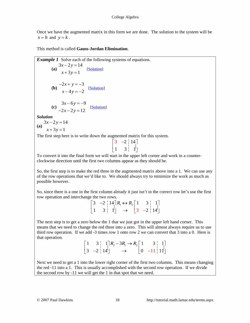
Once we have the augmented matrix in this form we are done. The solution to the system will be x h= and y k= . This method is called Gauss-Jordan Elimination. Example 1 Solve each of the following systems of equations.

(a) 3 2 14

3 1x yx y− =+ =

[Solution]

(b) 2 3

4 2x y

x y− + = −

− = − [Solution]

(c) 3 6 92 2 12

x yx y− = −

− − = [Solution]

Solution

(a) 3 2 14

3 1x yx y− =+ =

The first step here is to write down the augmented matrix for this system.

2 14

1 3 13 −

To convert it into the final form we will start in the upper left corner and work in a counter-clockwise direction until the first two columns appear as they should be. So, the first step is to make the red three in the augmented matrix above into a 1. We can use any of the row operations that we’d like to. We should always try to minimize the work as much as possible however. So, since there is a one in the first column already it just isn’t in the correct row let’s use the first row operation and interchange the two rows.

1 23 2 14 1 3 11 3 1 2 143

R R− ↔ → −

The next step is to get a zero below the 1 that we just got in the upper left hand corner. This means that we need to change the red three into a zero. This will almost always require us to use third row operation. If we add -3 times row 1 onto row 2 we can convert that 3 into a 0. Here is that operation.

2 1 21 3 1 3 1 3 113 2 14 0 11 1

R R R− → − → −

Next we need to get a 1 into the lower right corner of the first two columns. This means changing the red -11 into a 1. This is usually accomplished with the second row operation. If we divide the second row by -11 we will get the 1 in that spot that we need.

College Algebra


211 3 1 1 111

0 11 113

0 1 1R−

− − →

Okay, we’re almost done. The final step is to turn the red three into a zero. Again, this almost always requires the third row operation. Here is the operation for this final step.

1 2 11 3 1 3 1 0 40 1 1 0 1 1

R R R− → − → −

We have the augmented matrix in the required form and so we’re done. The solution to this system is 4x = and 1y = − .


(b) 2 3

4 2x y

x y− + = −

− = −

In this part we won’t put in as much explanation for each step. We will mark the next number that we need to change in red as we did in the previous part. We’ll first write down the augmented matrix and then get started with the row operations.

1 2 2 1 21 3 1 4 2 2 1 4 222 71 4 2 1 3 0 7

R R R R R− ↔ − − + → − − −

− − − − → − → −

Before proceeding with the next step let’s notice that in the second matrix we had one’s in both spots that we needed them. However, the only way to change the -2 into a zero that we had to have as well was to also change the 1 in the lower right corner as well. This is okay. Sometimes it will happen and trying to keep both ones will only cause problems. Let’s finish the problem.

1 2 1211 4 2 1 2 4 1 0 27

0 7 0 1 14

0 1 17R R RR− − − + →−

− → →

−−

The solution to this system is then 2x = and 1y = .


(c) 3 6 92 2 12

x yx y− = −

− − =

Let’s first write down the augmented matrix for this system.

6 9

2 2 123 − −

− −

Now, in this case there isn’t a 1 in the first column and so we can’t just interchange two rows as the first step. However, notice that since all the entries in the first row have 3 as a factor we can divide the first row by 3 which will get a 1 in that spot and we won’t put any fractions into the problem.

College Algebra


Here is the work for this system.

2 1 2116 9 1 2 3 2 1 2 33

2 2 12 2 122 6603 R R RR− − − − + → − −

− − − → − → −

( ) 1 2 1211 2 3 1 2 3 2 1 0

65

60 6 0 1 1 0 1 1

R R RR− − − + → −− − → − − →

−

The solution to this system is 5x = − and 1y = − .

[Return to Problems] It is important to note that the path we took to get the augmented matrices in this example into the final form is not the only path that we could have used. There are many different paths that we could have gone down. All the paths would have arrived at the same final augmented matrix however so we should always choose the path that we feel is the easiest path. Note as well that different people may well feel that different paths are easier and so may well solve the systems differently. They will get the same solution however. For two equations and two unknowns this process is probably a little more complicated than just the straight forward solution process we used in the first section of this chapter. This process does start becoming useful when we start looking at larger systems. So, let’s take a look at a couple of systems with three equations in them. In this case the process is basically identical except that there’s going to be more to do. As with two equations we will first set up the augmented matrix and then use row operations to put it into the form,

1 0 00 1 00 0 1

pqr

Once the augmented matrix is in this form the solution is x p= , y q= and z r= . As with the two equations case there really isn’t any set path to take in getting the augmented matrix into this form. The usual path is to get the 1’s in the correct places and 0’s below them. Once this is done we then try to get zeroes above the 1’s. Let’s work a couple of examples to see how this works.

College Algebra


Example 2 Solve each of the following systems of equations.

(a) 3 2 2

2 32 3 3

x y zx y zx y z

+ − =− + =− − =

[Solution]

(b) 3 2 72 2 9

3 6

x y zx y zx y z

+ − = −+ + =

− − + = [Solution]

Solution

(a) 3 2 2

2 32 3 3

x y zx y zx y z

+ − =− + =− − =

Let’s first write down the augmented matrix for this system.

1 2 2

1 2 1 32

3

1 3 3

− − − −

As with the previous examples we will mark the number(s) that we want to change in a given step in red. The first step here is to get a 1 in the upper left hand corner and again, we have many ways to do this. In this case we’ll notice that if we interchange the first and second row we can get a 1 in that spot with relatively little work.

1 2

332

1 2 2 1 2 1 31 2 1 3 1 2 22 1 3 3 1 3 3

R R− −

↔ − − → − − − −

The next step is to get the two numbers below this 1 to be 0’s. Note as well that this will almost always require the third row operation to do. Also, we can do both of these in one step as follows.

2 1 2

3 1 3

1 2 1 3 3 1 2 1 31 2 2 23 7

20 5 7

1 3 3 0 3 5 3

R R RR R R

− − → − − − → − − − − → − −

Next we want to turn the 7 into a 1. We can do this by dividing the second row by 7.

2

1 2 1 31 2 1 3 150 5 7 0 1 177

0 3 5 3 0 3

7

3 5

R− −

− − − − → − − − −

So, we got a fraction showing up here. That will happen on occasion so don’t get all that excited about it. The next step is to change the 3 below this new 1 into a 0. Note that we aren’t going to bother with the -2 above it quite yet. Sometimes it is just as easy to turn this into a 0 in the same step. In this case however, it’s probably just as easy to do it later as we’ll see.

College Algebra


So, using the third row operation we get,

3 2 3

1 2 1 3 1 2 1 335 50 1 1 0 1 1

7 70 5 33 0 020 0

7

R R R

− − − → − − − − → −

−−

Next, we need to get the number in the bottom right corner into a 1. We can do that with the second row operation.

3

157

20

1 2 1 3 1 2 37

50 1 1 0 1 1207

0 0 107

00 0

R

− − − − − − →

−

−

Now, we need zeroes above this new 1. So, using the third row operation twice as follows will do what we need done.

2 3 2

1 3 1

51 2 3 1 0 370 1 1 0 1 0 1

0 0 1 00 0

1571 0

2R R R

R R R

− + → − − → − →

−

−

Notice that in this case the final column didn’t change in this step. That was only because the final entry in that column was zero. In general, this won’t happen. The final step is then to make the -2 above the 1 in the second column into a zero. This can easily be done with the third row operation.

1 2 1

1 0 3 1 0 0 12

0 1 0 1 0 1 0 10 0 1 0 0 0 1 0

2R R R

+ → − − →

−

So, we have the augmented matrix in the final form and the solution will be, 1, 1, 0x y z= = − = This can be verified by plugging these into all three equations and making sure that they are all satisfied.


College Algebra


(b) 3 2 72 2 9

3 6

x y zx y zx y z

+ − = −+ + =

− − + =

Again, the first step is to write down the augmented matrix.

1 2 7

2 2 1 91 1 3

3

6

− − − −

We can’t get a 1 in the upper left corner simply by interchanging rows this time. We could interchange the first and last row, but that would also require another operation to turn the -1 into a 1. While this isn’t difficult it’s two operations. Note that we could use the third row operation to get a 1 in that spot as follows.

1 2 1

321

1 2 7 1 1 3 162 2 1 9 2 1 91 1 3 6 1 3 6

R R R− − − − −

− → → − − − −

Now, we can use the third row operation to turn the two red numbers into zeroes.

2 1 2

3 1 3

1 1 3 16 2 1 1 3 162 1 9 0 7 411 3 6 0 2 0 1

2 41 0

R R RR R R

− − − − → − − − + → −− → − −

The next step is to get a 1 in the spot occupied by the red 4. We could do that by dividing the whole row by 4, but that would put in a couple of somewhat unpleasant fractions. So, instead of doing that we are going to interchange the second and third row. The reason for this will be apparent soon enough.

2 3

1 1 3 16 1 1 3 160 7 41 0 0 100 2 0

4 210 0 4 7 41

R R− − − − − −

↔ − → − −

−

Now, if we divide the second row by -2 we get the 1 in that spot that we want.

2

1 1 3 16 1 1 3 1610 0 10 0 1 0 520 4 7 41 0 7 41

24

R− − − − − −

− − →

−

Before moving onto the next step let’s think notice a couple of things here. First, we managed to avoid fractions, which is always a good thing, and second this row is now done. We would have eventually needed a zero in that third spot and we’ve got it there for free. Not only that, but it won’t change in any of the later operations. This doesn’t always happen, but if it does that will make our life easier. Now, let’s use the third row operation to change the red 4 into a zero.

College Algebra


3 2 3

1 1 3 16 1 1 3 164

0 1 0 5 0 1 0 50 7 41 0 0 214 7

R R R− − − − − −

− → →

We now can divide the third row by 7 to get that the number in the lower right corner into a one.

3

1 1 3 16 1 1 1610 1 0 5 0 1 0 570 0 2 0

3

17 0 1 3

R− − − − −

→

−

Next, we can use the third row operation to get the -3 changed into a zero.

1 3

1 1 16 1 0 73

0 1 0 5 0 1 0 50 0 1 3 0 0 1 3

3 1R R R

− − − + →

→

− −

The final step is to then make the -1 into a 0 using the third row operation again.

1 2

1 0 7 1 0 0 20 1 0 5 0 1 0 50 0 1 3 0 0 1 3

1R R R

− − + →

→

−

The solution to this system is then, 2, 5, 3x y z= − = =

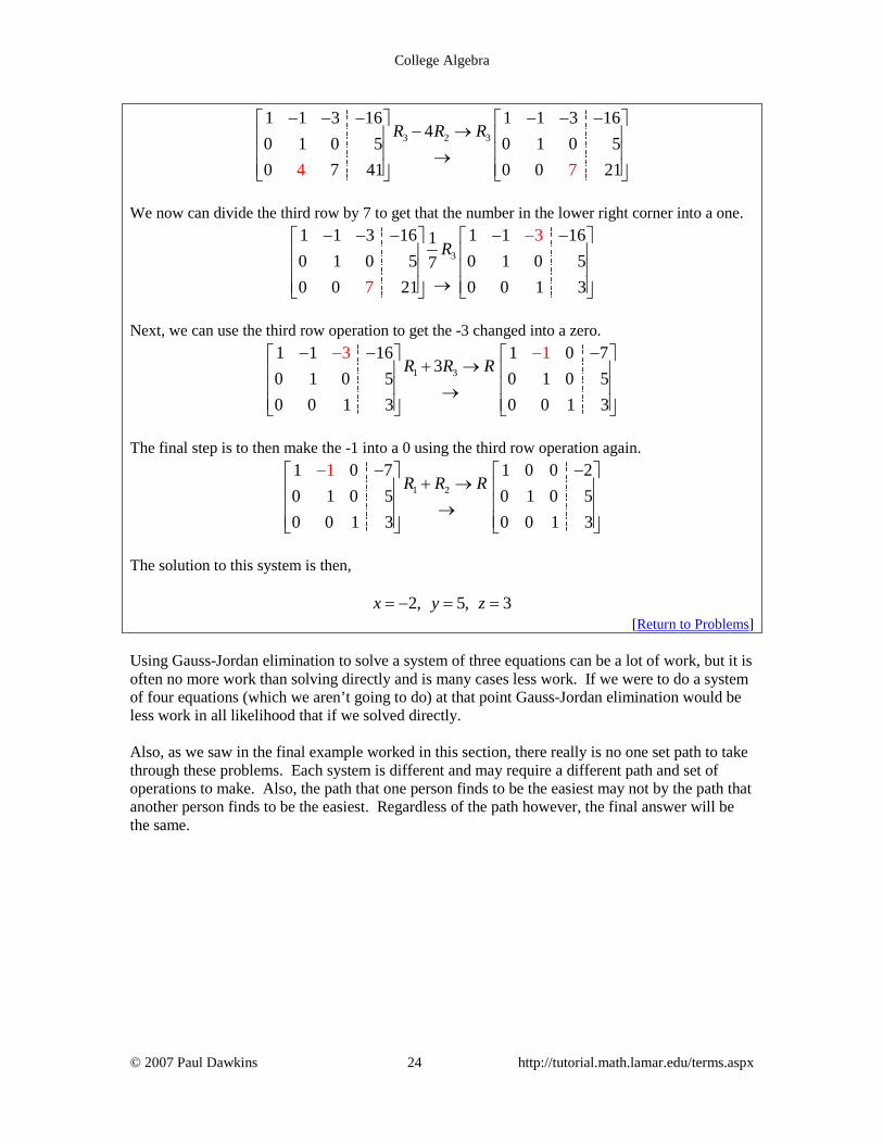
[Return to Problems] Using Gauss-Jordan elimination to solve a system of three equations can be a lot of work, but it is often no more work than solving directly and is many cases less work. If we were to do a system of four equations (which we aren’t going to do) at that point Gauss-Jordan elimination would be less work in all likelihood that if we solved directly. Also, as we saw in the final example worked in this section, there really is no one set path to take through these problems. Each system is different and may require a different path and set of operations to make. Also, the path that one person finds to be the easiest may not by the path that another person finds to be the easiest. Regardless of the path however, the final answer will be the same.

College Algebra


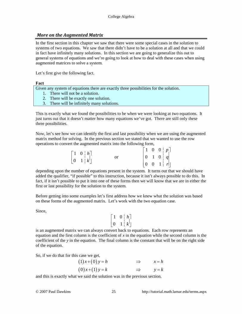
More on the Augmented Matrix In the first section in this chapter we saw that there were some special cases in the solution to systems of two equations. We saw that there didn’t have to be a solution at all and that we could in fact have infinitely many solutions. In this section we are going to generalize this out to general systems of equations and we’re going to look at how to deal with these cases when using augmented matrices to solve a system. Let’s first give the following fact. Fact Given any system of equations there are exactly three possibilities for the solution.

1. There will not be a solution. 2. There will be exactly one solution. 3. There will be infinitely many solutions.

This is exactly what we found the possibilities to be when we were looking at two equations. It just turns out that it doesn’t matter how many equations we’ve got. There are still only these three possibilities. Now, let’s see how we can identify the first and last possibility when we are using the augmented matrix method for solving. In the previous section we stated that we wanted to use the row operations to convert the augmented matrix into the following form,

1 0 0

1 0or 0 1 0

0 10 0 1

ph

qk

r

depending upon the number of equations present in the system. It turns out that we should have added the qualifier, “if possible” to this instruction, because it isn’t always possible to do this. In fact, if it isn’t possible to put it into one of these forms then we will know that we are in either the first or last possibility for the solution to the system. Before getting into some examples let’s first address how we knew what the solution was based on these forms of the augmented matrix. Let’s work with the two equation case. Since,

1 00 1

hk

is an augmented matrix we can always convert back to equations. Each row represents an equation and the first column is the coefficient of x in the equation while the second column is the coefficient of the y in the equation. The final column is the constant that will be on the right side of the equation. So, if we do that for this case we get,

( ) ( )( ) ( )1 0

0 1

x y h x h

x y k y k

+ = ⇒ =

+ = ⇒ =

and this is exactly what we said the solution was in the previous section.

College Algebra


This idea of turning an augmented matrix back into equations will be important in the following examples. Speaking of which, let’s go ahead and work a couple of examples. We will start out with the two systems of equations that we looked at in the first section that gave the special cases of the solutions. Example 1 Use augmented matrices to solve each of the following systems.

(a) 6

2 2 1x y

x y− =

− + = [Solution]

(b) 2 5 1

10 25 5x y

x y+ = −

− − = [Solution]

Solution

(a) 6

2 2 1x y

x y− =

− + =

Now, we’ve already worked this one out so we know that there is no solution to this system. Knowing that let’s see what the augmented matrix method gives us when we try to use it. We’ll start with the augmented matrix.

1 1 6

2 12−

−

Notice that we’ve already got a 1 in the upper left corner so we don’t need to do anything with that. So, we next need to make the -2 into a 0.

2 1 21 1 6 2 1 1 62 1 0 132 0

R R R− + → −−

→

Now, the next step should be to get a 1 in the lower right corner, but there is no way to do that without changing the zero in the lower left corner. That’s a problem, because we must have a zero in that spot as well as a one in the lower right corner. What this tells us is that it isn’t possible to put this augmented matrix form. Now, go back to equations and see what we’ve got in this case.

6

0 13 ???x y− =

=

The first row just converts back into the first equation. The second row however converts back to nonsense. We know this isn’t true so that means that there is no solution. Remember, if we reach a point where we have an equation that just doesn’t make sense we have no solution. Note that if we’d gotten

1 1 60 1 0

−

we would have been okay since the last row would return the equation 0y = so don’t get confused between this case and what we actually got for this system.


College Algebra


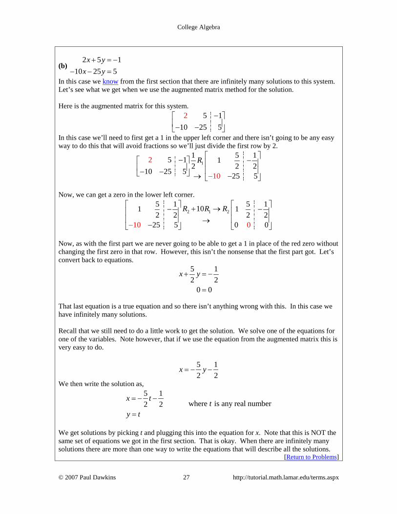
(b) 2 5 1

10 25 5x y

x y+ = −

− − =

In this case we know from the first section that there are infinitely many solutions to this system. Let’s see what we get when we use the augmented matrix method for the solution. Here is the augmented matrix for this system.

5 1

10 252

5−

− −

In this case we’ll need to first get a 1 in the upper left corner and there isn’t going to be any easy way to do this that will avoid fractions so we’ll just divide the first row by 2.

11 5 15 1 12 2 2

10 25 52

10 25 5

R − − − − → − −

Now, we can get a zero in the lower left corner.

2 1 25 1 5 1101 12 2 2 2

1 25 5 0 00 0

R R R + →− − →− −

Now, as with the first part we are never going to be able to get a 1 in place of the red zero without changing the first zero in that row. However, this isn’t the nonsense that the first part got. Let’s convert back to equations.

5 12 2

0 0

x y+ = −

=

That last equation is a true equation and so there isn’t anything wrong with this. In this case we have infinitely many solutions. Recall that we still need to do a little work to get the solution. We solve one of the equations for one of the variables. Note however, that if we use the equation from the augmented matrix this is very easy to do.

5 12 2

x y= − −

We then write the solution as,

5 1

where is any real number2 2x t

ty t

= − −

=

We get solutions by picking t and plugging this into the equation for x. Note that this is NOT the same set of equations we got in the first section. That is okay. When there are infinitely many solutions there are more than one way to write the equations that will describe all the solutions.


College Algebra


Let’s summarize what we learned in the previous set of examples. First, if we have a row in which all the entries except for the very last one are zeroes and the last entry is NOT zero then we can stop and the system will have no solution. Next, if we get a row of all zeroes then we will have infinitely many solutions. We will then need to do a little more work to get the solution and the number of equations will determine how much work we need to do. Now, let’s see how some systems with three equations work. The no solution case will be identical, but the infinite solution case will have a little work to do. Example 2 Solve the following system of equations using augmented matrices.

3 3 6 32 2 4 10

2 3 7

x y zx y z

x y z

− − = −− − =

− + + =

Solution Here’s the augmented matrix for this system.

3 6 3

2 2 4 102 3 1 7

3 − − − − − −

We can get a 1 in the upper left corner by dividing by the first row by a 3.

1

3 6 3 1 1 2 112 2 4 10 2 4 13

22

032 3 1 7 3 1 7

R− − − − − −

− − − − → − −

Next we’ll get the two numbers under this one to be zeroes.

2 1 2

3 1 3

1 1 2 1 2 1 1 2 12 4 10 2 0 0 0 123 1 7 0 3 52 1

2R R RR R R

− − − − → − − − − − + → → − −

And we can stop. The middle row is all zeroes except for the final entry which isn’t zero. Note that it doesn’t matter what the number is as long as it isn’t zero. Once we reach this type of row we know that the system won’t have any solutions and so there isn’t any reason to go any farther. Okay, let’s see how we solve a system of three equations with an infinity number of solutions with the augmented matrix method. This example will also illustrate an interesting idea about systems.

College Algebra


Example 3 Solve the following system of equations using augmented matrices. 3 3 6 32 2 4 2

2 3 7

x y zx y z

x y z

− − = −− − = −

− + + =

Solution Notice that this system is almost identical to the system in the previous example. The only difference is the number to the right of the equal sign in the second equation. In this system it is -2 and in the previous example it was 10. Changing that one number completely changes the type of solution that we’re going to get. Often this kind of simple change won’t affect the type of solution that we get, but in some rare cases it can. Since the first two steps of the process are identical to the previous part we won’t discuss them. Here they are.

2 1 2

13 1 3

3 6 3 1 1 2 1 2 1 1 2 112 2 4 2 2 4 2 2 0 0 0 032 3 1 7 3 1 7

22 5

3

0 1 3

R R RR

R R R− − − − − − − → − − −

− − − − − − + → → − → − −

We’ve got a row of all zeroes so we instantly know that we’ve got infinitely many solutions. Unlike the two equation case we aren’t going to stop however. It looks like with a couple of row operations we can make the second column look like it is supposed to in the final form so let’s do that.

2 3 1 2 1

1 1 2 1 1 2 1 1 0 5 40 0 0 0 1 3 5 0 1 3 50 1 3 5 0 0

10

0 0 0 0 0 0

R R R R R− − − − − −

→ + → − − → → −

−

In this case we were able to make the second column look like it’s supposed to and the third column will never look correct. However, it is possible that the situation could be reversed and it would be the third column that we can make look correct and the second wouldn’t look correct. Every system is different. Once we reach this point we go back to equations.

5 43 5

x zy z− =− =

Now, both of these equations contain a z and so we’ll move that to the other side in each equation.

5 43 5

x zy z= += +

This means that we get to pick the value of z for free and we’ll write the solution as,

College Algebra


5 43 5 where is any real number

x ty t tz t

= += +=

Since there are an infinite number of ways to choose t there are an infinite number of solutions to this system.

College Algebra


Non-Linear Systems In this section we are going to be looking at non-linear systems of equations. A non-linear system of equations is a system in which at least one of the variables has an exponent other than 1 and/or there is a product of variables in one of the equations. To solve these systems we will use either the substitution method or elimination method that we first looked at when we solved systems of linear equations. The main difference is that we may end up getting complex solutions in addition to real solutions. Just as we saw in solving systems of two equations the real solutions will represent the coordinates of the points where the graphs of the two functions intersect. Let’s work some examples. Example 1 Solve the following system of equations.

2 2 102 1

x yx y+ =+ =

Solution In linear systems we had the choice of using either method on any given system. With non-linear systems that will not always be the case. In the first equation both of the variables are squared and in the second equation both of the variables are to the first power. In other words, there is no way that we can use elimination here and so we are must use substitution. Luckily that isn’t too bad to do for this system since we can easily solve the second equation for y and substitute this into the first equation. 1 2y x= − ( )22 1 2 10x x+ − = This is a quadratic equation that we can solve.

( )( )

2 2

2

1 4 4 105 4 9 0

91 5 9 0 1,5

x x xx x

x x x x

+ − + =

− − =

+ − = ⇒ = − =

So, we have two values of x. Now, we need to determine the values of y and we are going to have to be careful to not make a common mistake here. We determine the values of y by plugging x into our substitution.

( )1 1 2 1 3x y= − ⇒ = − − =

9 9 131 25 5 5

x y = ⇒ = − = −

Now, we only have two solutions here. Do not just start mixing and matching all possible values of x and y into solutions. We get 3y = as a solution ONLY if 1x = − and so the first solution is,

1, 3x y= − =

College Algebra


Likewise, we only get 135

y = − ONLY if 95

x = and so the second solution is,

9 13,5 5

x y= = −

So, we have two solutions. Now, as noted at the start of this section these two solutions will represent the points of intersection of these two curves. Since the first equation is a circle and the second equation is a line have two intersection points is definitely possible. Here is a sketch of the two equations as a verification of this.

Note that when the two equations are a line and a circle as in the previous example we know that we will have at most two real solutions since it is only possible for a line to intersect a circle zero, one, or two times. Example 2 Solve the following system of equations.

2 22 2

2x y

xy− =

=

Solution Okay, in this case we have a hyperbola (the first equation, although it isn’t in standard form) and a rational function (the second equation if we solved for y). As with the first example we can’t use elimination on this system so we will have to use substitution. The best way is to solve the second equation for either x or y. Either one will give us pretty much the same work so we’ll solve for y since that is probably the one that will make the equation look more like those that we’ve looked at in the past. In other words, the new equation will be in terms of x and that is the variable that we are used to seeing in equations.

2yx

=

College Algebra


22

22

22

22 2

42 2

8 2

xx

xx

xx

− =

− =

− =

The first step towards solving this equation will be to multiply the whole thing by x2 to clear out the denominators.

4 2

4 2

8 22 8 0

x xx x

− =

− − =

Now, this is quadratic in form and we know how to solve those kinds of equations. If we define,

( )22 2 2 4u x u x x= ⇒ = = and the equation can be written as,

( )( )

2 2 8 04 2 0 2, 4

u uu u u u

− − =

− + = ⇒ = − =

In terms of x this means that we have the following,

2

2

4 2

2 2

x x

x x i

= ⇒ = ±

= − ⇒ = ±

So, we have four possible values of x and two of them are complex. To determine the values of y we can plug these into our substitution.

22 1222 12

x y

x y

= ⇒ = =

= − ⇒ = = −−

2

2

2 2 2 222 2 2 2

2 2 2 222 2 2 2

i i ix i yii i i

i i ix i yii i i

= ⇒ = = = = −

= − ⇒ = − = − = − =

For the complex solutions, notice that we made sure the i was in the numerator. The for solutions are then,

2, 1 and 2, 1 and2 22 , and 2 ,2 2

x y x yi ix i y x i y

= = = − = −

= = − = − =

College Algebra


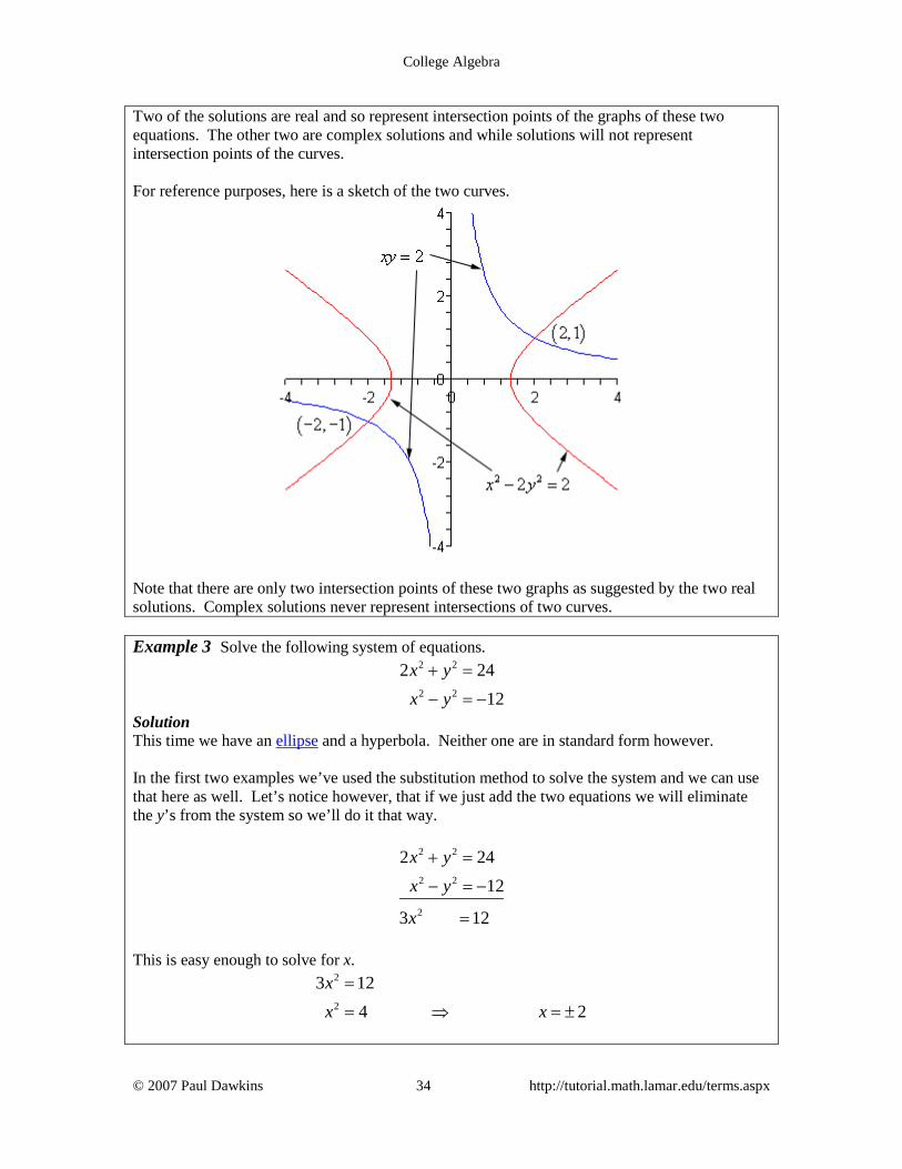
Two of the solutions are real and so represent intersection points of the graphs of these two equations. The other two are complex solutions and while solutions will not represent intersection points of the curves. For reference purposes, here is a sketch of the two curves.

Note that there are only two intersection points of these two graphs as suggested by the two real solutions. Complex solutions never represent intersections of two curves. Example 3 Solve the following system of equations.

2 2

2 2

2 2412

x yx y+ =

− = −

Solution This time we have an ellipse and a hyperbola. Neither one are in standard form however. In the first two examples we’ve used the substitution method to solve the system and we can use that here as well. Let’s notice however, that if we just add the two equations we will eliminate the y’s from the system so we’ll do it that way.

2 2

2 2

2

2 2412

3 12

x yx y

x

+ =

− = −

=

This is easy enough to solve for x.

2

2

3 124 2

xx x

=

= ⇒ = ±

College Algebra


To determine the value(s) of the y’s we can substitute these into either of the equations. We will use the first since there won’t be any minus signs to worry about.

2 :x =

( )2 2

2

2

2 2 24

8 2416 4

y

yy y

+ =

+ =

= ⇒ = ±

2 :x = −

( )2 2

2

2

2 2 24

8 2416 4

y

yy y

− + =

+ =

= ⇒ = ±

Note that for this system, unlike the previous examples, each value of x actually gave two possible values of y. That means that there are in fact four solutions. They are, ( ) ( ) ( ) ( )2,4 2, 4 2,4 2, 4− − − − This also means that there should be four intersection points to the two curves. Here is a sketch for verification.

college algebra - lamar universitytutorial.math.lamar.edu/dodownload.aspx?u=pdf/alg/... · college...

Documents