collision avoidance for vessels using a low-cost radar...

Collision Avoidance for Vessels using aLow-Cost Radar Sensor

Michael Schuster ∗ Michael Blaich ∗ Johannes Reuter ∗

∗University of Applied Sciences Konstanz, Konstanz, 78462 Germany(e-mail: schustem, mblaich, [email protected]).

Abstract: Collision avoidance for vessels highly depends on a robust obstacle detection. Thisis commonly achieved by use of high precision radar sensing. For smaller vessels however, theuse of low-cost sensors is typical. The idea of this work is to improve the robustness of collisionavoidance by integrating a sensor model together with the collision avoidance algorithm in orderto consider the accuracy of the measurements. Furthermore, a target tracking algorithm basedon an interacting Multi-Model Filter (IMM) is used for robust obstacle detection.

Keywords: Collision avoidance, Ship navigation, Path planning, COLREGs, Raster grid,Interacting Multiple Model Filter,

1. INTRODUCTION

Collision avoidance for vessels is an ongoing topic in ma-rine navigation research. In recent years, a lot of systemslike Automatic Identification System (AIS) and AutomaticRadar Plotting Aid (ARPA) have been developed to sup-port the ship navigators. Further, a multitude of collisionavoidance algorithms for scenarios on passages with highship traffic like the Baltic Sea or the English Channelhave been carried out. Most of these algorithms have beendeveloped for land based applications, specifically used inVessel Traffic Service (VTS) centers. These algorithms usethe AIS information of all vessels in the region of interest tocalculate optimal collision free routes for each vessel. How-ever, in a lot of areas e. g. inland lakes or coastal regions,plenty of vessels like recreational crafts operate withoutan AIS system. For such scenarios, on-board systems likeARPA are necessary to detect and track other vessels. AnARPA system estimates the risk of collision and proposesavoidance maneuvers to support the navigator. Neverthe-less, these systems are quit expensive, large, heavy, andhave high power consumption. Thus, they are unqualifiedfor smaller recreational crafts or small Unmanned ServiceVehicles (USV). The aim of this work is to present anon-board collision avoidance approach, which detects andtracks other vessels based on the measurements of a low-cost radar sensor and to use these tracks to calculate acollision free path for close range encounter situations.

The presented approach has been developed and tested onthe recreational craft ”Korona”, which is equipped witha Navico BR24 FMCW radar system, as shown in Fig. 1.The use of such a small, low-cost and low power consumingradar qualifies the approach for USVs and recreationalcrafts, particularly in regions where AIS carriage is notrequired. The test area is the Lake Constance and theupper Rhine river, where there is no obligation for AIScarriage. Because of the unavailability of AIS information,the position, course, speed, and dimensions of other vesselshave to be estimated by radar measurements and addi-

Fig. 1. The vessel Korona from the HTWG Konstanzequipped with the a Navico BR24 Radar Sensor.

tional algorithms to track the other vessels’ course. For thispurpose, an image preprocessing is used to detect objectsin the radar data. To estimate tracks associated withthese objects, a multiple model object tracking approachis applied. Based on these tracks, a collision avoidancealgorithm calculates a collision free path in real time. Thealgorithm respects the turning circle of the own vessel andprovides a drivable path according to the ”Rules of theRoad” (COLREGs, see (Benjamin et al., 2006)). This pathcould be used to support the vessel navigator or to guidethe vessel automatically.

In the last decades a multitude of algorithms concerningcollision avoidance for vessels have been carried out. Anoverview of the approach until 2009 is given in (Statheroset al., 2008; Tam et al., 2009). Referring to Tam et al.(2009), the most promising approach is an evolutionaryalgorithm presented by Smierzchalski (1999) but the mostpractical and efficient approach is the grid-based methodfrom Szlapczynski (2006). Nowadays, the algorithm forcollision avoidance can by divided in two groups. The first

Preprints of the 19th World CongressThe International Federation of Automatic ControlCape Town, South Africa. August 24-29, 2014

Copyright © 2014 IFAC 9673

Fig. 2. Raw radar image (left) and extracted radar targets(right). The colored targets are dolphins or ships. Thegray areas are considered to be part of the shore lineand will not be used for target tracking.

one consists of approaches which are developed to optimizethe vessel’s routes by land-based stations like Vessel TrafficServices (VTS). Most of these algorithms are based onthe approach of Smierzchalski (1999) and use heuristicoptimization methods to find optimal collision free routes.The most promising approach, therefore, is the hybridalgorithm presented in (Szlapczynski and Szlapczynska,2012). The second group comprises of methods that areused on-board the vessels. These methods use discretegrids to calculate a collision free path as presented in(Szlapczynski, 2006). Kuwata et al. (2013) presented anapproach based on a velocity space grid. They also showedsome results of actual on-water tests for multi vesselscenarios. In this work, the collision avoidance algorithmpresented in (Blaich et al., 2012a,b) is used to perform realon-water test.

2. RADAR DATA PREPROCESSING

The Navico BR24 FMCW radar system is an imagingsensor which provides a 360◦ echo image of the environ-ment every 2.5s. The image consists of 2048 range scans(spokes), one spoke approx. every 0.2◦ but with an openingbeam width of 5.2◦(3dB). Each spoke itself is split in 1024resolution cells, whose occupancy is indicated by a 4-bitvalue. The maximum range is configurable from 60m upto 32nmi. For the collision avoidance on inland waters wefocused our work on a maximum range of about 800m. Anexample is shown in Fig. 2. Each time, an image has beenreceived, the target extraction is performed in three steps:first an ego motion compensation, second a cell basedoccupancy likelihood determination and third a connectedcomponent labeling.

2.1 Ego Motion Compensation

In a first step, the effects of the own vessel’s yaw rateis compensated. This is done by calculating the azimuthof each scan in respect to the corresponding own vesselheading. The own vessel moves with low speed, only.Changes in the absolute position of the sensor are smallduring one scan and will be corrected in the trackingsystem.

2.2 Occupancy Likelihood Determination

Second, the occupancy likelihood of each resolution cellis determined. Because of the rather large beam width,in one spoke, several cells are affected for each rangestep. The returned energy to the radar is the sum ofthe energy reflected from all those cells. However, thereported amplitude is zero or maximum most of the time,and therefore, of rather little use. Thus, for any valuegreater than zero, a cell is assumed to be reported asoccupied. Based on the antenna beam width, we assumeeach cell becomes illuminated say n times during a 360◦-scan. Furthermore, we assume that for each spoke theprobability p of a cell being reported as occupied isindependent and constant. Thus, the occupancy likelihoodis binomially distributed and can be calculated by

Pr(ai,j = occ) =

m∑k=0

(n

k

)pk(1− p)n−k, (1)

where

m =

bn/2c∑l=b−n/2c

ai,j+l. (2)

Here, ai,j ∈ [0, 1] denotes the reported occupancy valueof each cell, i is the cell index in range and j in azimuth,respectively.

2.3 Connected Component Labeling

Finally, a cell is assumed to contain a target, if theoccupancy probability is greater than 0.5. Since a targetusually extends of several hundred cells, adjacent, occupiedcells are grouped using connected component labeling(Gonzalez and Woods, 2006). Each group is considered tobe a target of elliptical shape, for which range and azimuthof the center, its total size, cross range (distance betweenminimum and maximum bearing) and down range extends(distance between minimum range and maximum range)are calculated. The origin of each target is also verifiedusing a map, which was obtained previously, by extractingthe shore line from each radar scan (Greuter et al., 2012).Targets that are not located on the water are suppressed,and the remaining targets form the input of the MultiObject Tracking (Fig. 2).

3. TRACK FILTERING USING IMM

The extracted target positions are still very noisy, thus,strong low pass filtering is required to obtain an object’strue position, heading, and velocity. Using just one dy-namic model for straight line motion can lead to largeestimation errors or even track loss during a turning ma-neuver. Using only one model for maneuvering targets canlead to poor state estimates when the object keeps itsheading. Therefore, an interacting multiple model (IMM)filter is chosen here. The basic idea of this filter is torun several models in parallel. Based on the estimate ofeach model and the current measurement, a likelihood foreach model to reflect the true motion state is determined.The output of the filter is a weighted sum of all modelestimates. Since the IMM has been used in target trackingfor many years, only the used models and parameters areexplained here. For implementation details the reader is

19th IFAC World CongressCape Town, South Africa. August 24-29, 2014

9674

referred to Challa et al. (2011).

For each object on the water, three models of the form

x(i)k = f

(i)k

(x

(i)k−1

)+ G

(i)k w

(i)k (3)

are assumed. Here x(i)k is the state vector of the ith model

and f(i)k describes the corresponding system dynamics. w

(i)k

is a white noise sequence with zero mean and covariances

cov[w(i)k ] = Q(i), G

(i)k serves as an input matrix and

describes the interaction of the noise components with thestates. For prediction and measurement update of eachmodel, the Unscented Kalmanfilter is used (Julier andUhlmann, 2004). The models become time dependent dueto non constant sampling rate.

3.1 Dynamic Models

In the following, the dynamic models considered in thisstudy are explained briefly. Details concerning these mod-els can be found in Li and Jilkov (2003).

As straight line motion model the Constant Velocity(CV)model is applied. The state vector x(1) = (x, x, y, y)′,where x denotes the position along the own vessel lon-gitudinal axis and y the lateral axis. The process noise

Q(1) = diag[σ2x, σ

2y] reflects very small acceleration in both

direction.

The second model, used for maneuvering, is the ConstantTurn Rate and Velocity (CTRV) model. Here, the statex(2) = (x, y, ψ, ω, V )′ contains besides the position, theyaw angle ψ, turn rate ω. and the overall velocity V .It was already shown by Gertz (1989) that estimatingthe heading angle directly leads to better results duringa maneuver than estimating the corresponding velocitydirections. This model assumes that yaw rate and velocity

are nearly constant, with Q(2) = diag(σ2V , σ

2ω).

The last model is a Constant Acceleration (CA) modelwith state x(3) = (x, x, x, y, y, y)′. This model serves as atransition model, when the motion changes from straightline to constant turn or fast velocity changes occur. It usesthe same process noise expressions like the CV, but withhigher values for the variances.

3.2 Measurement Model

Since the utilized radar does not provide any Dopplerinformation, only the polar position measurements can beused for updating the dynamic models. The measurementequation is given by

zk =

[rθ

]= h (xk) + vk =

{ √x2 + y2

arctan(y/x)+ vk (4)

Here, vk is also normally distributed with zero mean andcovariance R = diag[σ2

R, σ2θ ].

For a collision avoidance system the size of an object isof critical importance. In Salmond and Parr (2003) a fifthstate is added to the CV model defining the length of anobject. It is assumed that all objects are of elliptical shapewith a fixed aspect ratio γ of major and minor axis. Thus,

the relationship between the measured down range LDRand the object length l is defined as

LDR(φ) = l

√cos2(φ) + γ2 sin2(φ), (5)

where the aspect angle φ = ψ − θ is the difference ofobject heading and measured azimuth. However, for oursystem, the measured down range is overestimated mostof the time and shows only little dependency on the aspectangle. Thus, we do not incorporate the object length inour dynamic models, but update the length estimate witha constant gain on every scan independently. The sameis done for the extracted size of the target, which is usedfor data association only. Due to the high antenna beamwidth, cross range values are in general too large to beof any use. When a new measurement is available, eachmodel is updated according to the rules of IMM. Basedon the individual filter residuals, a new model likelihoodis determined. The final state and uncertainty estimateis then given by the weighted sum of all models. Finally,the components of the object state necessary for the mostlikely model are provided for the path planning module,together with the length and the maneuvering likelihood.

4. TRACK HANDLING

One of the major challenge in a multi object trackingapplication still is the data association problem. In general,it is unknown which measurement was originated fromwhich object, even the cardinality of objects is not knowna priori. Especially when working with a radar on water,additional measurements occur which do not belong to anyreal object (clutter), or an existing object is not detected atall. To solve these problems, a large variety of algorithmshave been proposed. These can be roughly divided intotwo groups. The first group is comprised of single instancefilters. The states of all objects are collected in one set.This set is regarded as a new state space and is updatedusing one Bayes filter. The second group uses at least onefilter instance for each object. For these filters, an explicitmeasurement to object association has to be performed.Here also a large number of algorithms have been designedfor different applications and conditions.

For the presented application the following assumptionsare valid:

• One object creates just a single measurement.• Object trajectories can be in close proximity.

Because of these assumption, the Joint Probabilistic DataAssociation (JPDA) is selected, Bar-Shalom et al. (2005).The JPDA associates all measurements within a gate to atrack subject to all other tracks in this gate. To use theJPDA, first the assignment matrix A ∈ RMm×Mt has tobe calculated which contains for each measurement/trackpair the conditional measurement data likelihood. Mm

and Mt are the number of measurements that fall inthe gate, number of tracks in the gate, respectively. Formeasurement i and track j the association likelihood isassumed to be Gaussian distributed:

aij = N (zi, h(xj),Sj) i ∈ {1, . . . ,Mm}, j ∈ {1, . . . ,Mt}(6)

The innovation covariance Sj is the sum of the currenttrack position covariance and the constant measurement


9675

covariance. If the value is below some gating threshold,the likelihood is zero. Then, A has to be expanded foreach track by the likelihood of a missed detection, andfor each measurement the likelihood of false alarm or newobject likelihood has to be taken into account. Then, thejoint association likelihood is given by

p(aij) = aijper(Aij)

per(A)(7)

where the permanent is the sum of products over allpermutations:

per(A) =

n∑i=1

aijper(Aij) (8)

and Aij is the submatrix obtained by removing row i andcolumn j. The computation of all permanents can stillbe very time consuming. For this reason, they are herereplaced by an approximation. In Uhlmann (2008) variousapproximation schemes are compared with respect to theirassignment correctness. Based on these results, here theapproximation

per(A) ≤n∏i=1

n∑j=1

aijcicj

(9)

is adopted, where cj is the sum of column j. Based onthis aproximation, an optimal assignment approach is usedto find the measurement to track update pairing. Notassigned measurements are used as candidates for newtracks in the next update step.

5. COLLISION AVOIDANCE

The collisions avoidance algorithm uses the track informa-tion and the most probable model provided by the IMMfilter to predict the movement of the other vessels overa future time period. If the CTRV model is the mostprobable, the motion of the other vessel is predicted asan arc, otherwise it is predicted as a straight line. Thisinformation is used by the collision avoidance algorithmto find a safe path in close range encounter situations.The algorithm is divided in two steps. In the first step,a set of waypoints for a collision free path is estimatedin the local area. The size of this local region depends onthe sensor’s range. This algorithm is presented in detailin (Blaich et al., 2012a,b), thus, only a short overview ofthe algorithm is given in this section. In a second step thewaypoints are connected by Bezier splines to get a paththat is navigable by the vessel.

The algorithm for the waypoint search uses the own vesselspeed and course information to predict the own movementwhile traveling the local area. To predict the movement ofthe other vessels, the information provided by the trackingalgorithm is used. Both informations are stored in a gridto calculate the cost of a path. If map data is availablethis information is also stored in the same grid. To finda collision free path in this grid an A∗ search is used. Toconsider the own ship kinematic constraints, a special T-shape neighborhood is implemented. This neighborhoodonly considers those cells for the next search step thatare actually reachable by the vessel. For the other ships,a ship domain as presented by Goodwin (1975) is usedto prefer COLREGs compliant avoidance maneuvers. Theusage of the grid and the A∗ search enables the real-time

capability of the waypoint search, which is necessary foron-board systems.

For connecting the waypoints, Bezier splines are used insuch a way that the path segments are interconnectedwith continuous curvature. Thus, a smooth transitionbetween the segments is assured. Moreover, since the pathplanning algorithm already takes into account the vesselkinematics, the Bezier splines provide a continuous pathwith admissible curvature.

6. EXPERIMENTAL RESULTS

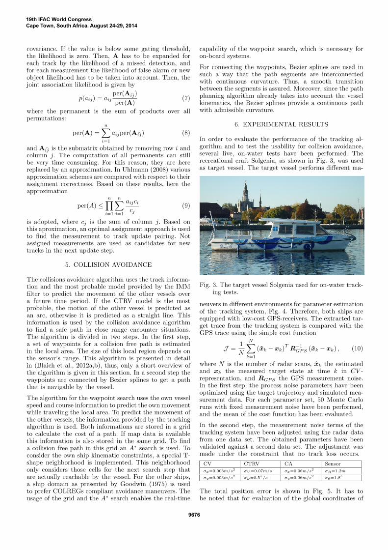
In order to evaluate the performance of the tracking al-gorithm and to test the usability for collision avoidance,several live, on-water tests have been performed. Therecreational craft Solgenia, as shown in Fig. 3, was usedas target vessel. The target vessel performs different ma-

Fig. 3. The target vessel Solgenia used for on-water track-ing tests.

neuvers in different environments for parameter estimationof the tracking system, Fig. 4. Therefore, both ships areequipped with low-cost GPS-receivers. The extracted tar-get trace from the tracking system is compared with theGPS trace using the simple cost function

J =1

N

N∑k=1

(xk − xk)TR−1GPS (xk − xk) , (10)

where N is the number of radar scans, xk the estimatedand xk the measured target state at time k in CV -representation, and RGPS the GPS measurement noise.In the first step, the process noise parameters have beenoptimized using the target trajectory and simulated mea-surement data. For each parameter set, 50 Monte Carloruns with fixed measurement noise have been performed,and the mean of the cost function has been evaluated.

In the second step, the measurement noise terms of thetracking system have been adjusted using the radar datafrom one data set. The obtained parameters have beenvalidated against a second data set. The adjustment wasmade under the constraint that no track loss occurs.

CV CTRV CA Sensor

σx=0.003m/s2 σV =0.07m/s σx=0.06m/s2 σR=1.2m

σy=0.003m/s2 σω=0.5◦/s σy=0.06m/s2 σθ=1.8◦

The total position error is shown in Fig. 5. It has tobe noted that for evaluation of the global coordinates of


9676

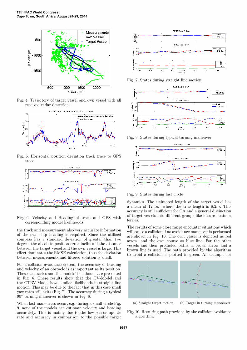
Fig. 4. Trajectory of target vessel and own vessel with allreceived radar detections

Fig. 5. Horizontal position deviation track trace to GPStrace

Fig. 6. Velocity and Heading of track and GPS withcorresponding model likelihoods.

the track and measurement also very accurate informationof the own ship heading is required. Since the utilizedcompass has a standard deviation of greater than twodegree, the absolute position error inclines if the distancebetween the target vessel and the own vessel is large. Thiseffect dominates the RMSE calculation, thus the deviationbetween measurements and filtered solution is small.

For a collision avoidance system, the accuracy of headingand velocity of an obstacle is as important as its position.These accuracies and the models’ likelihoods are presentedin Fig. 6. These results show that the CV-Model andthe CTRV-Model have similar likelihoods in straight linemotion. This may be due to the fact that in this case smallyaw rates still exits (Fig. 7). The accuracy during a typical90◦ turning maneuver is shown in Fig. 8.

When fast maneuvers occur, e.g. during a small circle Fig.9, none of the models can estimate velocity and headingaccurately. This is mainly due to the low sensor updaterate and accuracy in comparison to the possible target

Fig. 7. States during straight line motion

Fig. 8. States during typical turning maneuver

Fig. 9. States during fast circle

dynamics. The estimated length of the target vessel hasa mean of 12.4m, where the true length is 8.2m. Thisaccuracy is still sufficient for CA and a general distinctionof target vessels into different groups like leisure boats orferries.

The results of some close range encounter situations whichwill cause a collision if no avoidance maneuver is performedare shown in Fig. 10. The own vessel is depicted as redarrow, and the own course as blue line. For the othervessels and their predicted paths, a brown arrow and abrown line is used. The path provided by the algorithmto avoid a collision is plotted in green. An example for

(a) Straight target motion (b) Target in turning manoeuver

Fig. 10. Resulting path provided by the collision avoidancealgorithm.


9677

(a) (b) (c) (d)

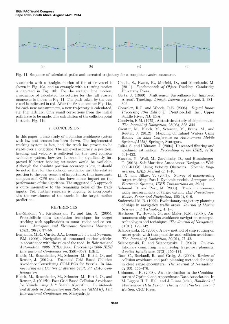
Fig. 11. Sequence of calculated paths and executed trajectory for a complete evasive maneuver.

a scenario with a straight motion of the other vessel isshown in Fig. 10a, and an example with a turning motionis depicted in Fig. 10b. For the straight line motion,a sequence of calculated trajectories for the full evasivemaneuver is shown in Fig. 11. The path taken by the ownvessel is indicated in red. After the first encounter Fig. 11a,for each new measurement, a new trajectory is calculated,e.g. Fig. 11b,11c. Only small corrections from the initialpath have to be made. The calculation of the collision pointis stable, Fig. 11d.

7. CONCLUSION

In this paper, a case study of a collision avoidance systemwith low-cost sensors has been shown. The implementedtracking system is fast, and the track has proven to bestable over a long time. The achieved accuracy in position,heading and velocity is sufficient for the used collisionavoidance system, however, it could be significantly im-proved if better heading estimates would be available.Although the absolute position accuracy is low, it shouldbe noted that for the collision avoidance just the relativeposition to the own vessel is of importance, thus inaccuratecompass and GPS resolution have minor impact on theperformance of the algorithm. The suggested CA approachis quite insensitive to the remaining noise of the trackinputs. Yet, further research is ongoing to incorporatealso the covariances of the tracks in the target motionprediction.

REFERENCES

Bar-Shalom, Y., Kirubarajan, T., and Lin, X. (2005).Probabilistic data association techniques for targettracking with applications to sonar, radar and eo sen-sors. Aerospace and Electronic Systems Magazine,IEEE, 20(8), 37–56.

Benjamin, M.R., Curcio, J.A., Leonard, J.J., and Newman,P.M. (2006). Navigation of unmanned marine vehiclesin accordance with the rules of the road. In Robotics andAutomation, 2006. ICRA 2006. Proceedings 2006 IEEEInternational Conference on, 3581–3587. IEEE.

Blaich, M., Rosenfelder, M., Schuster, M., Bittel, O., andReuter, J. (2012a). Extended Grid Based CollisionAvoidance Considering COLREGs for Vessels. In Ma-noeuvring and Control of Marine Craft, 9th IFAC Con-ference on.

Blaich, M., Rosenfelder, M., Schuster, M., Bittel, O., andReuter, J. (2012b). Fast Grid Based Collision Avoidancefor Vessels using A * Search Algorithm. In Methodsand Models in Automation and Robotics (MMAR), 17thInternational Conference on. Miezyzdroje.

Challa, S., Evans, R., Musicki, D., and Morelande, M.(2011). Fundamentals of Object Tracking. CambridgeUniversity Press.

Gertz, J. (1989). Multisensor Surveillance for ImprovedAircraft Tracking. Lincoln Laboratory Journal, 2, 381–396.

Gonzalez, R.C. and Woods, R.E. (2006). Digital ImageProcessing (3rd Edition). Prentice-Hall, Inc., UpperSaddle River, NJ, USA.

Goodwin, E.M. (1975). A statistical study of ship domains.The Journal of Navigation, 28(03), 328–344.

Greuter, M., Blaich, M., Schuster, M., Franz, M., andReuter, J. (2012). Mapping Of Inland Waters UsingRadar. In 22nd Conference on Autonomous MobileSystems(AMS). Springer, Stuttgart.

Julier, S. and Uhlmann, J. (2004). Unscented filtering andnonlinear estimation. Proceedings of the IEEE, 92(3),401–422.

Kuwata, Y., Wolf, M., Zarzhitsky, D., and Huntsberger,T. (2013). Safe Maritime Autonomous Navigation WithCOLREGS, Using Velocity Obstacles. Oceanic Engi-neering, IEEE Journal of, 1–10.

Li, X. and Jilkov, V. (2003). Survey of maneuveringtarget tracking. Part I: Dynamic models. Aerospace andElectronic Systems, IEEE Transactions on, 39(4).

Salmond, D. and Parr, M. (2003). Track maintenanceusing measurements of target extent. IEE Proceedings-Radar, Sonar and Navigation, 150(6), 0–6.

Smierzchalski, R. (1999). Evolutionary trajectory planningof ships in navigation traffic areas. Journal of MarineScience and Technology, 4, 1–6.

Statheros, T., Howells, G., and Maier, K.M. (2008). Au-tonomous ship collision avoidance navigation concepts,technologies and techniques. The Journal of Navigation,61(01), 129–142.

Szlapczynski, R. (2006). A new method of ship routing onraster grids, with turn penalties and collision avoidance.The Journal of Navigation, 59(01), 27–42.

Szlapczynski, R. and Szlapczynska, J. (2012). On evo-lutionary computing in multi-ship trajectory planning.Applied Intelligence, 37(2), 155–174.

Tam, C., Bucknall, R., and Greig, A. (2009). Review ofcollision avoidance and path planning methods for shipsin close range encounters. The Journal of Navigation,62(03), 455–476.

Uhlmann, J.K. (2008). An Introduction to the Combina-torics of Optimal and Approximate Data Association. InM. Liggins II, D. Hall, and J. Llinas (eds.), Handbook ofMultisensor Data Fusion: Theory and Practice, SecondEdition. CRC Press.


9678

collision avoidance for vessels using a low-cost radar...

Documents