HAL Id: hal-02908985https://hal.archives-ouvertes.fr/hal-02908985

Submitted on 29 Jul 2020

HAL is a multi-disciplinary open accessarchive for the deposit and dissemination of sci-entific research documents, whether they are pub-lished or not. The documents may come fromteaching and research institutions in France orabroad, or from public or private research centers.

L’archive ouverte pluridisciplinaire HAL, estdestinée au dépôt et à la diffusion de documentsscientifiques de niveau recherche, publiés ou non,émanant des établissements d’enseignement et derecherche français ou étrangers, des laboratoirespublics ou privés.

Collision-Free Transmissions in an IoT MonitoringApplication Based on LoRaWAN

Rahim Haiahem, Pascale Minet, Selma Boumerdassi, Leila Azouz Saidane

To cite this version:Rahim Haiahem, Pascale Minet, Selma Boumerdassi, Leila Azouz Saidane. Collision-FreeTransmissions in an IoT Monitoring Application Based on LoRaWAN. Sensors, MDPI, 2020,�10.3390/s20144053�. �hal-02908985�

sensors

Article

Collision-Free Transmissions in an IoT MonitoringApplication Based on LoRaWAN

Rahim Haiahem 1, Pascale Minet 2,* , Selma Boumerdassi 3 and Leila Azouz Saidane 1

1 RAMSIS Team, CRISTAL Laboratory, 2010 Campus University, 2010 Manouba, Tunisia;haiahem.rahim@gmail.com (R.H.); leila.saidane@ensi-uma.tn (L.A.S.)

2 EVA Project, Inria—Paris, 75012 Paris, France3 CEDRIC/CNAM, 75003 Paris, France; selma.boumerdassi@cnam.fr* Correspondence: pascale.minet@inria.fr

Received: 5 June 2020; Accepted: 16 July 2020; Published: 21 July 2020

Abstract: With the Internet of Things (IoT), the number of monitoring applications deployed isconsiderably increasing, whatever the field considered: smart city, smart agriculture, environmentmonitoring, air pollution monitoring, to name a few. The LoRaWAN (Long Range Wide AreaNetwork)architecture with its long range communication, its robustness to interference and itsreduced energy consumption is an excellent candidate to support such applications. However, if thenumber of end devices is high, the reliability of LoRaWAN, measured by the Packet Delivery Ratio(PDR), becomes unacceptable due to an excessive number of collisions. In this paper, we proposetwo different families of solutions ensuring collision-free transmissions. The first family is TDMA(Time-Division Multiple Access)-based. All clusters transmit in sequence and up to six end deviceswith different spreading factors belonging to the same cluster are allowed to transmit in parallel.The second family is FDMA (Frequency Divsion Multiple Access)-based. All clusters transmit inparallel, each cluster on its own frequency. Within each cluster, all end devices transmit in sequence.Their performance are compared in terms of PDR, energy consumption by end device and maximumnumber of end devices supported. Simulation results corroborate the theoretical results and show thehigh efficiency of the solutions proposed.

Keywords: IoT; LPWAN; LoRaWAN; monitoring application; reliability; scalability; collision-free;TDMA; FDMA; air pollution monitoring

1. Introduction

The Internet of Things (IoT) is tremendously contributing to the increase of the number ofmonitoring applications deployed. These applications belong to various fields like smart farming (withsmart irrigation, nutrient monitoring and disease detection) [1,2], air pollution monitoring [3,4], smartcities [5] (with smart parking, smart waste collection and smart lighting), environment control (withleak detection), etc. Such applications require long range transmissions (e.g., from 1 to 12 km), a highnumber (i.e., ≥900) of End Devices (EDs) transmitting short messages (i.e., less than 50 bytes) to a sinkin charge of gathering data, not frequently (e.g., from once every 5 mn, up to once every hour or every 6h). The high number of EDs deployed leads to the choice of low-cost wireless transceivers. In addition,since these devices are battery-operated, a high battery lifetime is required. Taking into account thefeatures of IoT monitoring applications, namely their monitoring area that ranges over an area of upto 6 km radius around the gateway, their data rate, the robustness against interferences and a highnetwork lifetime requested, the LoRaWAN solution [4,6] is the most attracting solution, compared withother examples of Low-Power WANs (LPWANs) such as Sigfox and NB-IoT (Narrow Band—Internetof Things)which enable long communication range and operate for long periods [7].

Sensors 2020, 20, 4053; doi:10.3390/s20144053 www.mdpi.com/journal/sensors

Sensors 2020, 20, 4053 2 of 33

However, many authors [8–12], observed that the reliability of LoRaWAN considerably decreaseswhen the number of EDs increases: the Packet Delivery Ratio (PDR) drops by 50% for 900 EDs.This scalability problem is an issue for LoRaWAN. The objective of this paper is to get rid of theunreliability of LoRaWAN due to collisions when the number of EDs increases. For that purpose,we propose and compare different solutions based on LoRaWAN [13] which ensure collision-freetransmissions for monitoring applications. The first solution, called OAPM_D for Orthogonal AirPollution Monitoring Deterministic solution, is based on a time division multiple access (TDMA) ofclusters, where a cluster is a group of EDs, whereas the second solution, called FAPM for FDMA-basedAir Pollution Monitoring solution, is based on a frequency division multiple access (FDMA) of clusters.These basic solutions are optimized to support more End Devices (EDs) without losing messages andare compared on five different configurations, with uniform distribution of spreading factors or not.The evaluation criteria are: (i) the number of EDs supported, (ii) the reliability of the networkingsolution evaluated by the Packet Delivery Ratio, (iii) the energy consumed by each ED, (iv) the EDlifetime, (v) the time needed to collect the monitoring report of all EDs. To get quantitative performanceresults, an air pollution monitoring application is considered for an illustrative purpose, and the formatof the air pollution monitoring report is given. More generally, the solutions proposed are valid for anyIoT monitoring application where each ED has a monitoring report to transmit once per monitoringperiod. We also discuss the applicability of these solutions according to the application requirementsin terms of latency, number of EDs deployed and monitoring area size.

This paper is organized as follows. In Section 2, we present some IoT monitoring applications insmart agriculture, smart cities and environment monitoring. The LoRaWAN architecture is describedas well as some solutions dealing with the unreliability of LoRaWAN. Section 3 defines the frameworkof this study. OAPM-D, a TDMA-based solution, and its optimized variant OAPM-O are detailed inSection 4, whereas Section 5 deals with FAPM, a FDMA-based solution, and its optimized variantFAPM-O. These solutions are compared from a theoretical point of view and then by simulation.In Section 6, the air pollution monitoring application is used for an illustrative purpose to evaluate theperformances of our solutions. Theoretical and simulation results confirm the very good reliabilityobtained for a high maximum number of EDs. Complexity, ED energy consumption, network lifetimeand data gathering delay are evaluated. In Section 7, the applicability of these solutions is discussedwith regard to the IoT application requirements. A hybrid solution minimizing the gathering delay isproposed in Section 8. Finally, Section 9 summarizes the main results and gives some perspectives.

2. Related Work

2.1. IoT Monitoring Applications

IoT monitoring applications are various. They are already deployed in smart agriculture,smart cities, environment monitoring, etc. In [1], the authors present a review of long-range (LoRa)and (LoRaWAN)-enabled IoT applications for smart agriculture. They analyze the currently availablelong-range wide-area network technologies that could be the most appropriate for agriculture andagri-tech applications. Since in the agri-tech context, End Devices (EDs) usually monitor and reportenvironmental factors such as temperature, humidity, and chemical conditions of soil and plantsthat do not require up-to-date real-time monitoring, authors conclude that LoRaWAN technology isthe most suitable competitor for this type of application. Thus, the paper discusses the limits andoutstanding research limitations of LoRaWAN and points out the biggest challenge and issue ofthe future development of large-scale LoRaWAN applications: the effect of packet collision on thedeployment scalability.

In [14], the authors develop an IoT agriculture system based on LoRaWAN. The system is madeup of three services: the data collection service, the data analytics service and a remote control service.EDs transmit their measures to the LoRaWAN gateways (GWs) which transmit them to The ThingsNetwork (TTN) platform used to register EDs. GWs reroute the formatted messages to the cloud

Sensors 2020, 20, 4053 3 of 33

services. The cloud is in charge of data storage, data analytics and visualization. As a proof of concept,authors positioned three collector nodes (EDs) and one executor nodes in a 1-km radius from the GW.Air temperature, humidity and soil moisture measured by EDs are used by the analytics service todecide about the irrigation system. The decision is sent to the executor of the watering pump in thefield, in order to turn it on or off, according to the decision received.

In [15], the authors present a long term evaluation of LoRaWAN for smart city IoT deployments.The paper details experiences from deploying a city-scale LoRaWAN network across Southampton, UK.The aims behind this deployment are to support an installation of air quality monitoring and to explorethe capabilities of LoRaWAN protocol. Furthermore, the authors compare different LoRaWAN nodesand Gateways needed for the deployment. Based on the data-set produced over 135,000 transmissionsgathered while monitoring air quality, the authors analyze message delivery reliability and delay,as well as the scheduling and the atmospheric influences on message delivery. Finally, authors assertthat LoRaWAN is an applicable communication technology for city-scale air quality monitoring andother smart city applications.

In [16], the authors aim to demonstrate the feasibility of an Air Quality (AQ) monitoring systembased on Internet of Things (IoT) devices. Each IoT device is equipped with several sensors able tosense the variations in time and space of Particulate Matter (PM) air pollutants. Power and networkconnectivity are provided by a Power Over Ethernet (PoE) HAT to a Raspberry Pi 3 Model B. Each IoTdevice results in a total cost of approximatively 900 USD (with four PM sensors supported per device)in its first version and approximatively 1000 USD (up to ten PM sensors supported per device) inthe second one. To allow low bandwidth and long range communication, a LoRaWAN module hasbeen included. Six IoT devices were deployed in two school sites in Southampton to monitor PMconcentration over a period of seven months. Results show that on the one hand, the Spreading Factor(SF) 10 gives the best trade-off in terms of range and throughput. On the other hand, the capability ofthese IoT devices to sense spatio-temporal variations of air pollutants with a lower cost than this of anAutomatic Urban and Rural Network (AURN) station is established.

In [3], the authors present a real-life 100-day deployment of low-cost black carbon (BC) sensorsacross 100 distinct sampling locations in the 15 km2 neighborhood in West Oakland, California.The residents, organizations and businesses were recruited to host Aerosol Black Carbon Detector(ABCD) units. Data from the sampling location is aggregated in an online database containing 1-minuteaverage black carbon (BC) concentration measurements wirelessly transmitted by each ABCD andstored in a custom SQL database online. BC concentration measurements were collected over a periodof 240,000 h and used to raise awareness of the harmful effects of air pollution on health.

2.2. LoRaWAN and Its Reliability Problem

As seen in the previous subsection, many authors agree on the fact that LoRaWAN meets manyrequirements of IoT monitoring applications. We now briefly present LoRaWAN, before pointing outits reliability problem and summarizing some solutions based on a time slotted medium access.

LoRa uses the chirp spread spectrum (CSS) modulation to provide a long-range communicationlink robust to interference [17]. According to the ERC Recommendation 70-03 [18], LoRa operates inthe 868 MHz band in Europe and in the 915 MHz band in North America. Table 1 presents LoRaWANdefault channels and duty cycle limitations for the 868 MHz band, where each channel has a bandwidthof 125 kHz. LoRa supports different transmission bitrates depending on the Spreading Factor (SF)used. The SF value ranges from 7 with the highest bitrate of 5470 bps and a distance up to 2 km, to 12with the lowest bit rate of 250 bps and a distance up to 6 km in urban area [6]. The main advantage inthis modulation is that several transmissions with different SFs on the same channel are orthogonaland can be received simultaneously by the GW, provided that they are allowed by the number ofreceive paths [19,20].

Sensors 2020, 20, 4053 4 of 33

Table 1. LoRaWAN default channels and duty cycle limitations.

Channel Central Frequency (MHz) Duty Cycle Regulatory Regime Max Effective Radiated Power (ERP)

1 868.12 868.3 1% h 1.5 14 dBm3 868.5

4 868.85 0.1% h 1.6 14 dBm5 869.05

6 869.525 10% h 1.7 27 dBm

LoRaWANTM [13] defines the architecture of a network based on LoRa. There are three maintypes of devices: Network Server (NS), Gateways (GWs) and End Devices (EDs). The EDs form a startopology around the GW. All EDs transmit their messages to the GW according to the Aloha mediumaccess method. Three different classes of EDs exist, namely:

• Class A devices, with the basic set of features that all devices must implement. Hence, class A isthe default class with the lowest power consumption class [7].

• Class B devices, in addition to the functionalities of Class A, can be accessed by the GW at somepredefined time slots defined by Beacon messages periodically sent by the gateway [11].

• Class C devices are Continuously listening End Devices. Hence, they are accessible withlow-latency but consume more energy than EDs of any other class [10].

The complexity GW forwards the messages received from the EDs to the cloud-based NetworkServer via standard IP connections. Because of its multi-channel transceiver, the GW is able tosimultaneously receive several messages on multiple channels (i.e., up to eight channels).

The complexity is kept within the NS [13] with the elimination of redundant received packets,security checks, acknowledgment and downlink traffic scheduling, data rate adaptation, etc.

Many authors, [12,21–23], observed that when the number of End Devices (EDs) increases,the Packet Delivery Ratio (PDR) of LoRaWAN falls below the ratio acceptable by the application.This is due to the high number of collisions arising with the Aloha medium access method. In [23],the authors study the performance of LoRaWAN especially to find network capacity and understandhow transmission reliability depends on the number of packets generated by the end devices.Assuming that the messages are generated according to a Poisson distribution, the comparison of thedeveloped mathematical model and the simulation reveals that the collisions resolution approach usedin LoRaWAN is inefficient with a high number of EDs. In order to limit the collision, the authors showwith simulation that when the transmission frequency is 10 Hz and the biggest payload size of thegreatest SF used is 51 bytes, the communication is rather reliable (packet loss ratio less than 0.001) ifthe number of EDs is 100 and each ED sends at most one packet per 20 min. The network capacitymay reach 5000 EDs when each of them generates two messages per day on average.

Our paper aims at proposing solutions to avoid collisions, whereas others try to strongly limitthem [23] or transform them into constructive collisions like Choir [24] or QuAiL [25] using the linearaddition of powers of phase-asynchronous channels. Others take advantage of specific hardware tosuccessfully decode weak transmissions at the GW, like Charm [26].

2.3. Solutions Based on Time Slots

Several solutions to improve the reliability of LoRaWAN, such as [8,9,27], rely on a time slottedmedium access. In [27], the authors propose to regulate the medium access within slots (Slotted Aloha).For this purpose, they introduce a time synchronization service for low-cost IoT LoRaWAN devicesconnected to a gateway. When any ED transmits a confirmed uplink frame, it includes its timestampat the end of its transmission. The GW sends a timestamped Acknowledgement in the RX1 receivewindow. Thus, the ED has all the information needed for clock re-alignment. The authors developedand deployed a LoRaWAN testbed in real-life conditions. They show that their solution improves thereliability in real-life deployments based on LoRaWAN.

Sensors 2020, 20, 4053 5 of 33

In [8], each End Device is assigned a time slot, whose value is computed from its own address andthe frame length. The last slot of the frame is used by the GW on the one hand, to synchronize the EDsand on the other hand, to group the acknowledgments of transmissions sent in this frame. The framelength dynamically evolves over time to reflect the real number of EDs in the LoRaWAN network.

In [9], time slots are assigned to End Devices (EDs) according to their traffic needs.The synchronization and scheduling methods are triggered by any ED to get its time slot indexesencoded in Bloom filters to reduce the size of scheduling messages. They show that this solutionimproves the reliability of LoRaWAN. However, the scalability problem remains for a large number ofdevices, or even a moderate number of devices but with high SFs.

3. Framework for Performance Evaluation

3.1. Notations

In this paper, we adopt the notations given in Table 2.

Table 2. Notations.

MA Monitoring Application

GW GatewayED End DeviceNS Network Sever

F Number of frequency channels the GW simultaneously listens to, F = 3, 6 or 8M Maximum number of messages simultaneously demodulated by the GW, also

called number of receive paths of the GW, M = 8

SP Synchronization PeriodMP Monitoring PeriodTW Time WindowTT Transmission Time∆ The clock of any ED is synchronized within ∆ to the GW clock

SG Synchronization guard time between a downlink synchronization messagefollowed by an uplink monitoring message, or vice-versa

MG Monitoring guard time between two uplink monitoring messages

SF Spreading Factor, SF ∈ {7, 8, 9, 10, 11, 12}TSF Transmission Time of a monitoring message using the spreading factor SF

EDOAPMD Maximum number of EDs supported by OAPM_DEDFAPM Maximum number of EDs supported by FAPM

3.2. General Architecture

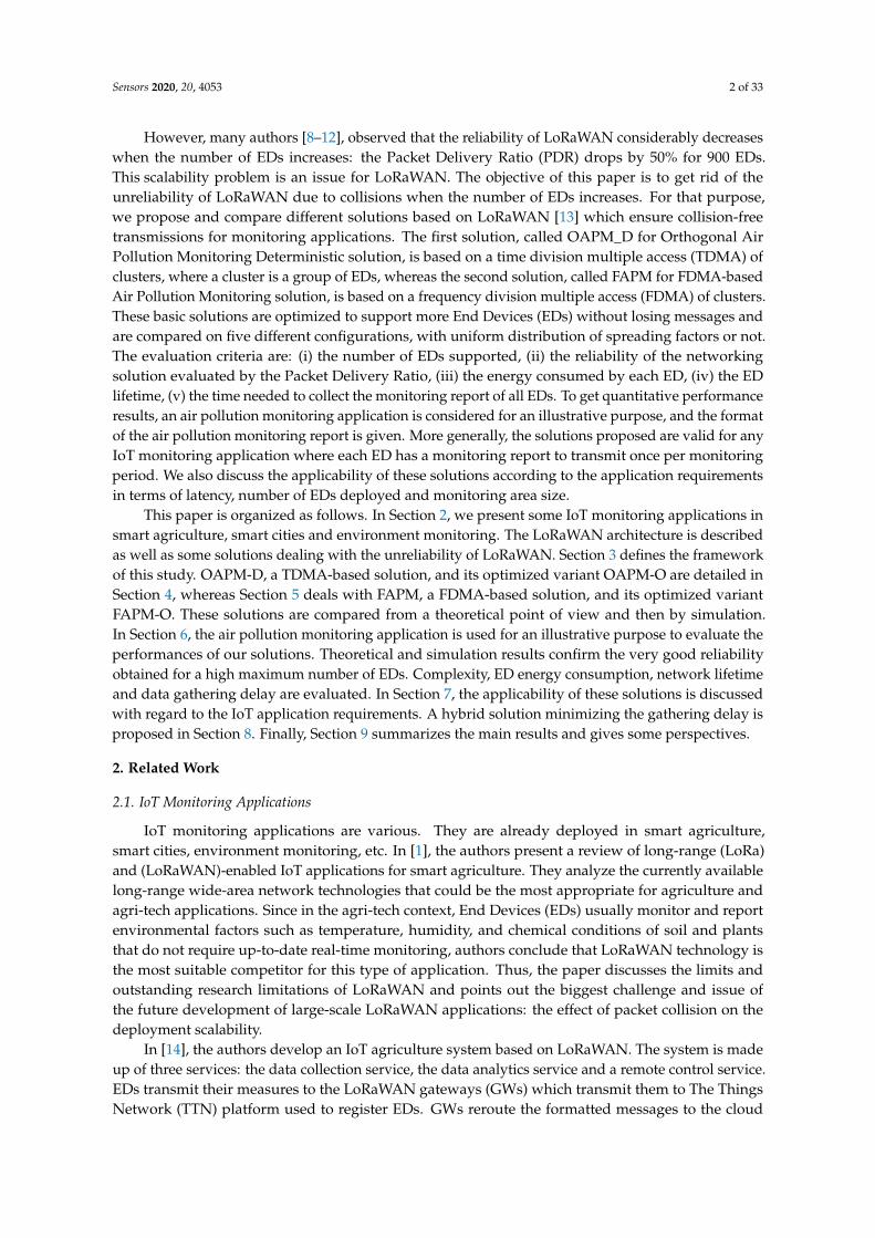
An example of LoRaWAN architecture is depicted in Figure 1. The monitoring area consists offive clusters represented by the five disks and populated by End Devices (EDs). Each ED is representedby a small dot whose color refers to the Spreading Factor (SF) used by this ED. The meaning of thenumber associated with the ED in Figure 1 depends on the solution proposed. For instance, it can bethe identifier of the ED sub-cluster, or the frequency used by this ED.

More generally, the architecture for the LoRaWAN network supporting monitoring applicationscan be described as follows:

A1 A single gateway (GW) exists in the monitoring area. It is located in the center of the monitoringarea to reduce its distance to EDs, whose activity is ruled by their duty cycle limitation (i.e., 1%).

A2 This gateway has a number of frequency channels F = 3, 6 or 8. Three is the default number,whereas eight is the maximum number of frequency channels that a commercially available GWcan listen to, see for instance the technical features of the SX1301 digital baseband chip [6].

Sensors 2020, 20, 4053 6 of 33

A3 The gateway can simultaneously demodulate several messages using different spreading factorseven on the same frequency channel. However, the gateway cannot demodulate more than M = 8messages simultaneously [6]. M is also called the number of receive paths in the literature.

A4 The monitoring area is split into angular sectors centered at the gateway as depicted in Figure 1.Each angular sector is called a cluster. Clusters are populated by End Devices (EDs), according totheir geographical coordinates obtained when the EDs are deployed.

A5 All EDs are LoRaWAN [13] class A devices, which is the basic class and the most energy-efficientone.

A6 All EDs are one-hop away from the GW. In other words, the network topology is a star centeredat the GW.

A7 Each ED uses a spreading factor SF ∈ {SF7, SF8, SF9, SF10, SF11, SF12} that depends on itsdistance to the GW.

A8 Each ED transmits a single message per monitoring period, denoted MP. This message containsits monitoring report. This uplink traffic is not acknowledged (i.e., unconfirmed data type).

A9 Each ED transmits its monitoring message at a time and on a frequency channel assigned by theNetwork Server according to the solution considered (e.g., Algorithm 1 for FAPM in Section 5).

A10 All EDs are synchronized with regard to the reference time of the GW. All EDs are keptsynchronized within ∆ from the GW. The synchronization period is denoted SP.

Figure 1. General network architecture with 5 clusters in the monitoring area.

It is worth noting that all the solutions proposed in this paper rely on Transmission Times assignedby the Network Server to EDs to ensure collision-free transmissions. However, this is not sufficient toavoid overlapping transmissions of two successive transmissions made by two different EDs, since theclocks of EDs drift apart over time. To get rid of this problem, EDs are periodically synchronized to thereference time provided by the GW and two guard periods are introduced:

Sensors 2020, 20, 4053 7 of 33

• SG the synchronization guard to avoid either the overlapping of either a previous uplinktransmission and the downlink synchronization message, or the overlapping of a previousdownlink synchronization message and an uplink transmission.

SG = ∆ + max_propagation_delay (1)

• MG the monitoring guard to avoid overlapping of two successive uplink transmissions made bytwo different EDs.

MG = 2∆ + max_propagation_delay (2)

Several synchronization algorithms exist. Some adopt an on-demand approach, where each EDtransmits its synchronization request to the GW. To reduce the energy consumption, simple algorithmssynchronizing all the EDs in one-shot are preferred such as [28,29].

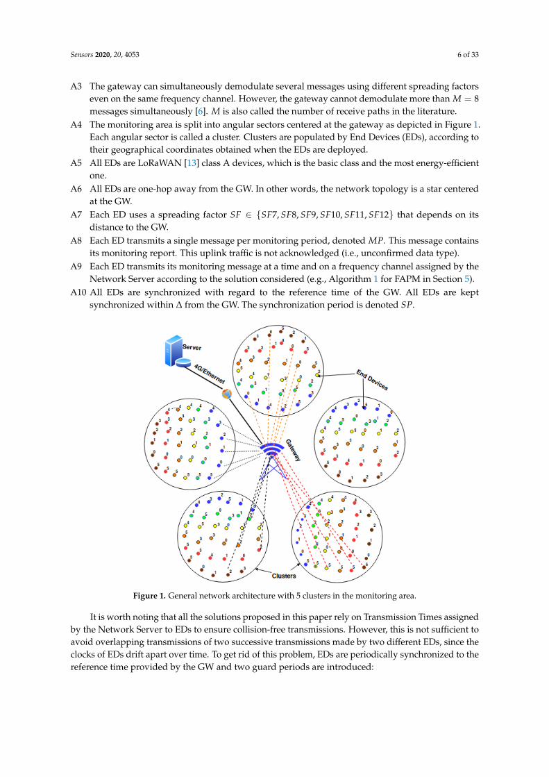
Hence, the medium activity over time is organized into synchronization periods, as depicted inFigure 2, where Sync denotes the synchronization message and MR the monitoring report message.

Figure 2. Medium activity over time.

Each synchronization period is delimited by the transmission of two successive synchronizationmessages. After the transmission of the synchronization message, several monitoring periods follow.A monitoring period consists of several Time Windows. Each cluster in the monitoring area is assigneda Time Window and one or several frequencies to transmit the monitoring reports of its EDs. Each EDis assigned a Transmission Time within the Time Window of its cluster and one frequency amongthose assigned to its cluster. Those assignments are such that all transmissions are collision-free.As a consequence, the following two constraints should be met:

Constraint C1: The synchronization period contains nMPperSP monitoring periods with nMPperSP ≥1:

TSync + 2SG + nMPperSP×MP ≤ SP, (3)

where TSync is the Transmission on Air of the synchronization message.Constraint C2: The monitoring period allows each ED to transmit its monitoring report without

collisions. The expression of this constraint depends on the solution adopted(e.g., OAPM_D, FAPM, etc.).

3.3. Performance Evaluation Criteria and Additional Assumptions

In the comparative performance evaluation, we focus more particularly on the air pollutionmonitoring application. The air pollution level is evaluated by measuring the Air Quality Index(AQI) according to the recommendations given by the World Health Organization [30] and the USEnvironmental Protection Agency [31]. The AQI has six levels of air pollution with different impacts

Sensors 2020, 20, 4053 8 of 33

on the environment and people; these levels are Good, Moderate, Unhealthy for sensitive groups,Very Unhealthy and Hazardous. Six major pollutants have been identified as the causes of air pollution:Carbon Monoxide CO, Nitrogen Dioxide NO2, Sulfur Dioxide SO2, Ozone O3, Particulate Matter PM2.5

and Particulate Matter PM10. The concentration of pollutant is averaged over one hour for O3, SO2

and NO2, and over 24 h for Particulate Matter PM2.5 and PM10.For the performance evaluation, we adopt some additional assumptions, which are not required

by OAPM_D and FAPM, but make the performance computation easier (e.g., A11, A12), or allowa quantitative evaluation of the maximum number of EDs supported (e.g., A13 and A14):

A11 All clusters have the same distribution of SFs.A12 The synchronization message is broadcast with the maximum SF used in the configuration

considered. It has a total size of 17 bytes, where 4 bytes are used for the GW timestamp.A13 The synchronization period is set to 1602 s, corresponding to a maximum propagation delay of

18 µs [32] associated with a radius of 6 km around the GW, SG = 1.018 ms, MG = 2.018 ms and∆ = 1 ms. The monitoring period varies from 400 s to 1600 s.

A14 The monitoring report transmitted by each End Device (ED) has a message size of 21 bytes. Inthe monitoring message, each index of the six main air pollutants is coded on 10 bits, leading to8 bytes of payload and a total of 21 bytes for the Monitoring message.

The deployment of the GW has to take into account multiple constraints: the real topography,the urban buildings and health rules, to name a few. This may result in various configurations wherethe GW is close to its EDs, or on the contrary, far from its EDs. To have a quantitative performanceevaluation representative of various real-world deployments, we evaluate the LoRaWAN-basedsolutions proposed on five configurations, which are:

• C16,16,16,16,16,16 A uniform configuration where the distribution of EDs within the monitoring areais uniform with regard to the different spreading factors. Each SF in {7,8,9,10,11,12} is used by100/6 = 16.66% of the EDs in the monitoring area. Intuitively, this configuration has the samenumber of EDs in each concentric crown of width R around the GW, where R is the radio range ofthe smallest spreading factor. This means that the number of EDs with high spreading factorsper unit of surface is reduced compared to the number of EDs with small spreading factors.It corresponds to a constant distribution of SFs.

• C10,20,20,20,20,10 A non-uniform distribution where the minimum and the maximum SFs (i.e., SF7and SF12) are used by 10% of the EDs, whereas the other SFs are used by 20% of the EDs.This configuration is close to the uniform one, except that the number of EDs very close and thenumber of EDs very far are smaller. This corresponds to a one-step distribution of SFs.

• C33,33,33,0,0,0 A non-uniform distribution where the only SFs present in the monitoring area areSF7, SF8 and SF9, in the same ratio. This configuration corresponds to a “best case” deployment,where all EDs are close to the GW.

• C0,0,0,33,33,33 A non-uniform distribution where the only SFs present in the monitoring areaare SF10, SF11 and SF12, in the same ratio. This configuration corresponds to a “worst case”deployment, where all EDs are far from the GW, which could not be installed closer to the EDs fordiverse reasons.

• C5,15,35,30,10,5 a non-uniform distribution where all SFs are present but with different percentages.SF7 is used by 5% of EDs, SF8 by 15%, SF9 by 35%, SF10 by 30%, SF11 by 10% and SF12 by5%. This configuration corresponds to a deployment, where some EDs are very close to the GWwhereas others are very far, but most of them are at a medium distance from the GW. The SFdistribution shape is closer to a bell.

For each configuration, we evaluate the maximum number of EDs supported by OAPM_D,FAPM and their optimized variants, both by theoretical computation and by simulation. For theoreticalresults, we use the assumption A11 (i.e., all clusters have the same distribution as the monitoring area)

Sensors 2020, 20, 4053 9 of 33

to define the concept of representative of the ED distribution in the different SFs. A representativeis a set of EDs with their associated SFs, such that each cluster contains a multiple of representatives.We evaluate the transmission time of a representative with each solution to deduce the maximumnumber of EDs per cluster.

4. OAPM_D, A TDMA-Based Solution

4.1. Presentation of OAPM_D

In OAPM_D, clusters are subdivided into sub-clusters and each cluster transmits sequentially,similarly for the sub-clusters. The parallelism of transmissions is obtained within each sub-clusterwhere a number of EDs equal to the number of different SFs in this sub-cluster, transmits in parallel.In any case, each sub-cluster includes at most six EDs, which is the maximum number of different SFspresent in this sub-cluster. OAPM_D is a deterministic solution where each ED within a sub-clustertransmits on a given frequency channel and at a transmission time given by the network server.The scheme of transmissions with OAPM_D is depicted in Figure 3, where the clusters are representedby disks, sub-clusters by dashed ovals and EDs by dots whose color represents their spreading factor.Each cluster i transmits sequentially in the time window TWi assigned to it. Similarly, the sub-clustersof cluster i transmit sequentially in TWi. All the EDs belonging to the same cluster (i.e., at most sixEDs) have different SFs and transmit simultaneously, which is illustrated by the six receive paths RPkat the bottom of Figure 3, where RPk denotes the kth receive path of the GW.

Figure 3. Time diagram of transmissions with OAPM_D.

In OAPM_D, the choice of the frequency channel used by any ED is assigned by the NetworkServer, in such a way that at any time, there is at most one ED transmitting its message on a givenfrequency channel using a given SF. For OAPM_D, Constraint C2 leads to:

nsub

∑h=1

(Th + MG) ≤ MP (4)

where nsub denotes the number of sub-clusters in the monitoring area and Th is the maximumtransmission time on the air of a monitoring report with the maximum spreading factor in sub-clusterh.

Notice that in specific configurations, where some receive paths of the GW would remain unusedbecause some spreading factors are missing in the cluster considered, some optimizations are possible.

Sensors 2020, 20, 4053 10 of 33

For instance in configurations C33,33,33,0,0,0 and C0,0,0,33,33,33, two EDs using the same SF could begrouped into the same sub-cluster provided that they are assigned two different frequency channels(see Sections 4.3.3 and 4.3.4 for more details). This is the intuitive idea behind OAPM_O.

4.2. Presentation of OAPM_O

OAPM_O is the optimized version of OAPM_D, where the main principles of OAPM_D are kept:clusters and sub-clusters transmit sequentially, but EDs in the same sub-cluster transmit in parallel onthe frequency channel and with the SF assigned by the Network Server. The definition of sub-cluster isgeneralized to allow the coexistence of several EDs using the same SF in the same sub-cluster, providedthat they transmit on different frequency channels. This condition is required to ensure collision-freetransmissions.

Notice that GW cannot listen to more than F channels with 3 ≤ F ≤ 8 and can demodulate atmost M = 8 messages simultaneously [6]. Hence, in OAPM_O, the number of EDs per sub-clustermay be higher than 6 which is the maximum allowed in OAPM_D. As a consequence, the number ofEDs supported by OAPM_O is greater than or equal to that supported by OAPM_D, as we will see inthe next section.

4.3. Theoretical Performances of OAPM_D and OAPM_O

4.3.1. Configuration C16,16,16,16,16,16

In the C16,16,16,16,16,16 configuration, each cluster contains the same number of EDs for each SFin [7, 12]. Hence, the representative is SF7, SF8, SF9, SF10, SF11, SF12. Since F the number of GWreceive paths is at least equal to 6, each sub-cluster in the OAPM family contains exactly six EDs withsix different SFs to guarantee collision-free transmissions. The number of sub-clusters in a cluster is

limited by:⌊

MPT12+MG

⌋. Hence the maximum number of EDs supported by OAPM_D and OAPM_O is

given by:

EDOAPMD = EDOAPMO = 6×⌊

MPT12 + MG

⌋, (5)

where T12 denotes the Time on Air of the monitoring report using SF12.

4.3.2. Configuration C10,20,20,20,20,10

In the C10,20,20,20,20,10 configuration, each cluster contains the same number of EDs for eachSF in [8, 11] and this number is twice the number of EDs with SF7, which is also the numberof EDs with SF12. As a consequence, a representative of the cluster distribution is given by:SF7, SF8, SF9, SF10, SF11, SF12, SF8, SF9, SF10, SF11. The number of representatives in the monitoringarea should be such that each ED is able to transmit once per monitoring period without a collision.Since by definition of OAPM_D, EDs with SF7 to SF12 can transmit in parallel (one ED per SF), the timeneeded by a representative to transmit is equal to T12 + T11 + 2MG. Hence, the maximum number of

representatives is given by⌊

MPT12+T11+2MG

⌋. Since, each representative contains 10 EDs, the maximum

number of EDs supported by OAPM_D and OAPM_O is given by:

EDOAPMD = EDOAPMO = 10×⌊

MPT12 + T11 + 2MG

⌋. (6)

4.3.3. Configuration C33,33,33,0,0,0

In the C33,33,33,0,0,0 configuration, each cluster contains only EDs with SF in {7, 8, 9} and has thesame number of EDs for each SF in {7, 8, 9}. Hence, a representative of cluster distribution is givenby SF7, SF8, SF9. However, when at least two frequency channels are available, OAPM_O uses two

Sensors 2020, 20, 4053 11 of 33

frequency channels per sub-cluster allowing two EDs with the same SF to transmit simultaneously,but on two different channel frequencies. Hence with this improvement, a cluster representative, whichis also a sub-cluster representative, consists of two EDS using SF7, two EDs using SF8, and two EDsusing SF9. One ED with SF7, one ED of SF8 and one ED of SF9 transmit in parallel on a given channel,where the three others EDs of this sub-cluster transmit in parallel on another given channel. Thetransmission time required by a representative to transmit its message is given by T9 + MG. Hence, the

maximum number of cluster representatives is given by⌊

MPT9+MG

⌋. Since, each representative contains

six EDs, the maximum number of EDs supported by OAPM_O is given by:

EDOAPMO = 6×⌊

MPT9 + MG

⌋. (7)

whereas the number of EDs supported by OAPM_D is only

EDOAPMD = 3×⌊

MPT9 + MG

⌋. (8)

4.3.4. Configuration C0,0,0,33,33,33

The case of the C0,0,0,33,33,33 configuration is very similar to the previous one, leading to thefollowing maximum number of EDs supported by OAPM_O:

EDOAPMO = 6×⌊

MPT12 + MG

⌋. (9)

whereas the number of EDs supported by OAPM_D is only

EDOAPMD = 3×⌊

MPT12 + MG

⌋. (10)

4.3.5. Configuration C5,15,35,30,10,5

In the C5,15,35,30,10,5 configuration, a cluster distribution representative is given bySF7, 3SF8, 7SF9, 6SF10, 2SF11, SF12, leading to one sub-cluster with SF7 . . . SF12, one sub-cluster withSF8 . . . SF11, one sub-cluster with SF8 . . . SF10, three sub-clusters with SF9, SF10 and one sub-clusterwith SF9. These sub-clusters have a total transmission time equal to T12 + T11 + 4× T10 + T9 + 7MG.

Hence, the maximum number of representatives per cluster is given by⌊

MPT12+T11+4×T10+T9+7MG

⌋.

Since, each representative contains 20 EDs, the maximum number of EDs supported by OAPM_D isgiven by:

EDOAPMD = 20×⌊

MPT12 + T11 + 4× T10 + T9 + 7MG

⌋. (11)

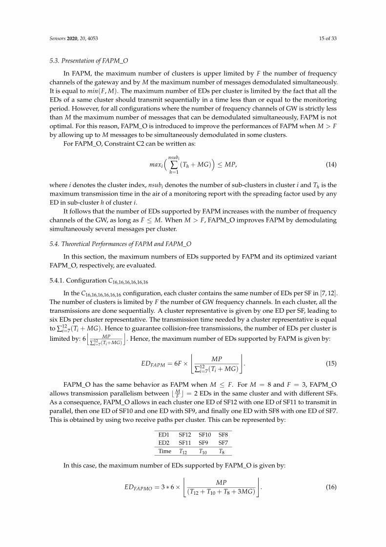
With OAPM_O, the idea consists in filling each sub-cluster with M EDs, while ensuring that atmost F frequency channels and at most M receive paths are used. The sub-cluster membership isgiven in Table 3, where members of any sub-cluster are denoted in black, blue or red, depending onthe frequency channel assigned to transmit the ED monitoring reports (i.e., a frequency channel isrepresented by a color: black, blue or red). We notice that increasing F from 3 to 6 or 8 does not changethe membership of clusters, since each sub-cluster 1 or 2 already transmits M messages in parallel andconsumes all the available receive paths of the GW.

Sensors 2020, 20, 4053 12 of 33

Table 3. Sub-cluster versus number of frequency channels for OAPM_O.

Channels Sub-Clusters Members Transmission Duration

3, 6 or 8 1 SF7, SF8, SF9, SF10, SF11, SF12, SF9, SF10 T12 + MG2 SF8, SF9, SF10, SF11, SF9, SF10, SF9, SF10 T11 + MG3 SF8, SF9, SF10, SF9 T10 + MG

EDOAPMO = 20×⌊

MPT12 + T11 + T10 + 3MG

⌋. (12)

4.4. Discussion

Note that in OAPM_D, if the number of frequency channels of the GW is strictly higher than themaximum number of different SFs present in the sub-cluster, some frequency channels remain unused.To increase the maximum number of EDs supported, there are several possibilities. The first one hasalready been presented, it consists in optimizing the definition of sub-clusters by allowing two EDs withthe same SF to coexist, provided that they use two different frequency channels. Another possibilityconsists in assigning different frequency channels to clusters, enabling them to transmit in parallel.This is the basic idea of FAPM presented in the next section.

5. FAPM, A FDMA-Based Solution

5.1. Description of FAPM

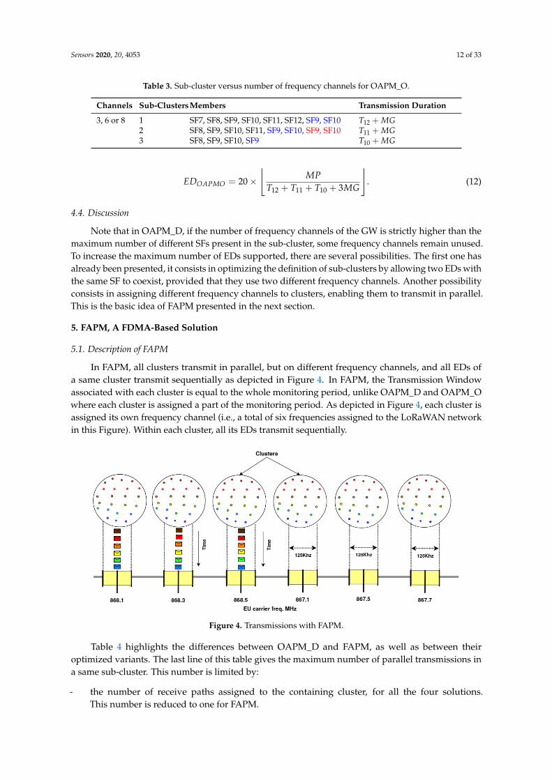
In FAPM, all clusters transmit in parallel, but on different frequency channels, and all EDs ofa same cluster transmit sequentially as depicted in Figure 4. In FAPM, the Transmission Windowassociated with each cluster is equal to the whole monitoring period, unlike OAPM_D and OAPM_Owhere each cluster is assigned a part of the monitoring period. As depicted in Figure 4, each cluster isassigned its own frequency channel (i.e., a total of six frequencies assigned to the LoRaWAN networkin this Figure). Within each cluster, all its EDs transmit sequentially.

Figure 4. Transmissions with FAPM.

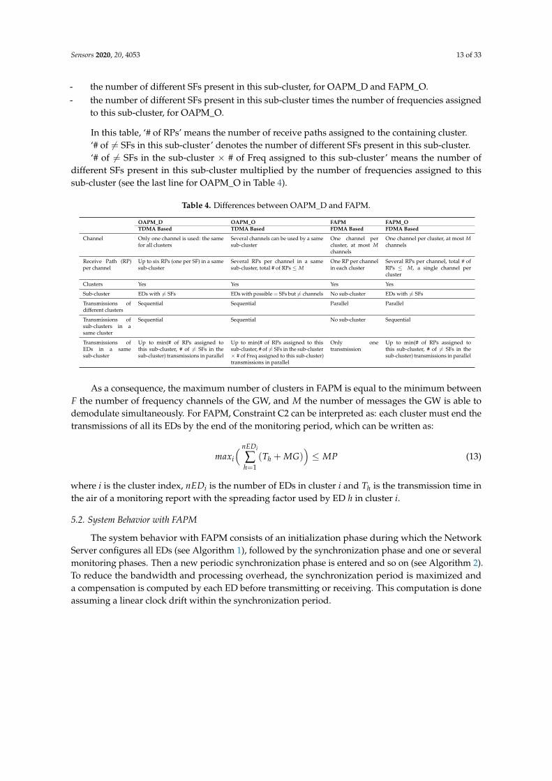
Table 4 highlights the differences between OAPM_D and FAPM, as well as between theiroptimized variants. The last line of this table gives the maximum number of parallel transmissions ina same sub-cluster. This number is limited by:

- the number of receive paths assigned to the containing cluster, for all the four solutions.This number is reduced to one for FAPM.

Sensors 2020, 20, 4053 13 of 33

- the number of different SFs present in this sub-cluster, for OAPM_D and FAPM_O.- the number of different SFs present in this sub-cluster times the number of frequencies assigned

to this sub-cluster, for OAPM_O.

In this table, ‘# of RPs’ means the number of receive paths assigned to the containing cluster.‘# of 6= SFs in this sub-cluster’ denotes the number of different SFs present in this sub-cluster.‘# of 6= SFs in the sub-cluster × # of Freq assigned to this sub-cluster’ means the number of

different SFs present in this sub-cluster multiplied by the number of frequencies assigned to thissub-cluster (see the last line for OAPM_O in Table 4).

Table 4. Differences between OAPM_D and FAPM.

OAPM_D OAPM_O FAPM FAPM_OTDMA Based TDMA Based FDMA Based FDMA Based

Channel Only one channel is used: the samefor all clusters

Several channels can be used by a samesub-cluster

One channel percluster, at most Mchannels

One channel per cluster, at most Mchannels

Receive Path (RP)per channel

Up to six RPs (one per SF) in a samesub-cluster

Several RPs per channel in a samesub-cluster, total # of RPs ≤ M

One RP per channelin each cluster

Several RPs per channel, total # ofRPs ≤ M, a single channel percluster

Clusters Yes Yes Yes Yes

Sub-cluster EDs with 6= SFs EDs with possible = SFs but 6= channels No sub-cluster EDs with 6= SFs

Transmissions ofdifferent clusters

Sequential Sequential Parallel Parallel

Transmissions ofsub-clusters in asame cluster

Sequential Sequential No sub-cluster Sequential

Transmissions ofEDs in a samesub-cluster

Up to min(# of RPs assigned tothis sub-cluster, # of 6= SFs in thesub-cluster) transmissions in parallel

Up to min(# of RPs assigned to thissub-cluster, # of 6= SFs in the sub-cluster× # of Freq assigned to this sub-cluster)transmissions in parallel

Only onetransmission

Up to min(# of RPs assigned tothis sub-cluster, # of 6= SFs in thesub-cluster) transmissions in parallel

As a consequence, the maximum number of clusters in FAPM is equal to the minimum betweenF the number of frequency channels of the GW, and M the number of messages the GW is able todemodulate simultaneously. For FAPM, Constraint C2 can be interpreted as: each cluster must end thetransmissions of all its EDs by the end of the monitoring period, which can be written as:

maxi

( nEDi

∑h=1

(Th + MG))≤ MP (13)

where i is the cluster index, nEDi is the number of EDs in cluster i and Th is the transmission time inthe air of a monitoring report with the spreading factor used by ED h in cluster i.

5.2. System Behavior with FAPM

The system behavior with FAPM consists of an initialization phase during which the NetworkServer configures all EDs (see Algorithm 1), followed by the synchronization phase and one or severalmonitoring phases. Then a new periodic synchronization phase is entered and so on (see Algorithm 2).To reduce the bandwidth and processing overhead, the synchronization period is maximized anda compensation is computed by each ED before transmitting or receiving. This computation is doneassuming a linear clock drift within the synchronization period.

Sensors 2020, 20, 4053 14 of 33

Algorithm 1 End Devices Configuration (Run by the server to configure all End Devices)

/* Initializations */for each ED in the monitored area do

/* Cluster assignment */Assign ED to a cluster according to its geographic coordinates obtained during deploymentCompute minSF and maxSF the minimum and maximum SF used in the network

end for/* Compute the parameters common to all EDs */

Initialize SP, MP, SP_Start, MP1← SG + TSync, nMPperSP, maxSF/* Compute the transmission and receive times of all EDs */

for each RP = 1 to M do

I(RP)← 1 /* Initialize the transmission index per receive path */end forfor each cluster in the monitored area do

for each ED ∈ cluster do

/* Assign a receive path to each ED and an index on this receive path */ED.RP← a receive path ∈ [1, M]Index ← I(RP)I(RP) + +/* Assign Transmission Time to this ED */ED.TT ← ∑Index−1

k=1 Tk + (Index− 1)MG /* From the beginning of the monitoring period */end for /* ED */

end for /* Cluster *//* Send configuration parameters to all EDs */

for SF = minSF to maxSF do

Uncon f igured← all the EDs using SFwhile Uncon f igured 6= empty do

Multicast configuration parameters to a maximum number of EDs ∈ Uncon f igured using SFRemove these EDs from Uncon f igured

end whileend for

Algorithm 2 Monitoring step (Run by any End Device ED)

Receive (ConfigurationParameters)Initialize its local parametersNextAwake← SP_StartNbS = 0 /* Number of the current synchronization period */repeat

/* Behavior of any ED during a synchronization period */Sleep until NextAwake to receive the next synchronization messageProcess the synchronization message,Update the clockComp← the compensation before next transmitNbS ++NextAwake← SP_Start + MP1 + ED.TT + Compfor NbM = 1 to nMPperSP do

/* Transmit its monitoring report once per MPduring nMPperSP successive periods */Sleep until NextAwake to transmit its monitoring msgBuild the air pollutant reportTransmit the air pollutant report to the GWComp← the compensation before next transmitNextAwake← SP_Start + MP1 + NbM ∗MP + ED.TT + Comp

end forComp← the compensation before next receiptNextAwake← SP_Start + NbS ∗ SP + Comp

until forever

Sensors 2020, 20, 4053 15 of 33

5.3. Presentation of FAPM_O

In FAPM, the maximum number of clusters is upper limited by F the number of frequencychannels of the gateway and by M the maximum number of messages demodulated simultaneously.It is equal to min(F, M). The maximum number of EDs per cluster is limited by the fact that all theEDs of a same cluster should transmit sequentially in a time less than or equal to the monitoringperiod. However, for all configurations where the number of frequency channels of GW is strictly lessthan M the maximum number of messages that can be demodulated simultaneously, FAPM is notoptimal. For this reason, FAPM_O is introduced to improve the performances of FAPM when M > Fby allowing up to M messages to be simultaneously demodulated in some clusters.

For FAPM_O, Constraint C2 can be written as:

maxi

( nsubi

∑h=1

(Th + MG))≤ MP, (14)

where i denotes the cluster index, nsubi denotes the number of sub-clusters in cluster i and Th is themaximum transmission time in the air of a monitoring report with the spreading factor used by anyED in sub-cluster h of cluster i.

It follows that the number of EDs supported by FAPM increases with the number of frequencychannels of the GW, as long as F ≤ M. When M > F, FAPM_O improves FAPM by demodulatingsimultaneously several messages per cluster.

5.4. Theoretical Performances of FAPM and FAPM_O

In this section, the maximum numbers of EDs supported by FAPM and its optimized variantFAPM_O, respectively, are evaluated.

5.4.1. Configuration C16,16,16,16,16,16

In the C16,16,16,16,16,16 configuration, each cluster contains the same number of EDs per SF in [7, 12].The number of clusters is limited by F the number of GW frequency channels. In each cluster, all thetransmissions are done sequentially. A cluster representative is given by one ED per SF, leading tosix EDs per cluster representative. The transmission time needed by a cluster representative is equalto ∑12

i=7(Ti + MG). Hence to guarantee collision-free transmissions, the number of EDs per cluster is

limited by: 6⌊

MP∑12

i=7(Ti+MG)

⌋. Hence, the maximum number of EDs supported by FAPM is given by:

EDFAPM = 6F×⌊

MP

∑12i=7(Ti + MG)

⌋. (15)

FAPM_O has the same behavior as FAPM when M ≤ F. For M = 8 and F = 3, FAPM_Oallows transmission parallelism between bM

F c = 2 EDs in the same cluster and with different SFs.As a consequence, FAPM_O allows in each cluster one ED of SF12 with one ED of SF11 to transmit inparallel, then one ED of SF10 and one ED with SF9, and finally one ED with SF8 with one ED of SF7.This is obtained by using two receive paths per cluster. This can be represented by:

ED1 SF12 SF10 SF8ED2 SF11 SF9 SF7Time T12 T10 T8

In this case, the maximum number of EDs supported by FAPM_O is given by:

EDFAPMO = 3 ∗ 6×⌊

MP(T12 + T10 + T8 + 3MG)

⌋. (16)

Sensors 2020, 20, 4053 16 of 33

5.4.2. Configuration C10,20,20,20,20,10

In the C10,20,20,20,20,10 configuration, the number of EDs with SF = 7 and the number ofEDs with SF12 represent 10% of the total number of EDs, whereas the number of EDs withany other SF represents 20% of the total number of EDs. In such a case, each ED patternSF7, SF8, SF9, SF10, SF11, SF12, SF8, SF9, SF10, SF11 needs a time equal to ∑12

i=7(Ti + MG)+∑11i=8(Ti +

MG) to transmit the pollutant reports. Hence the maximum number of EDs per cluster is given by

10×⌊

MP12

∑i=7

(Ti + MG) +11

∑i=8

(Ti + MG)

⌋. Since there is one cluster per frequency channel of the GW,

the maximum number of EDs supported by FAPM is given by:

EDFAPM = 10F×⌊

MP

∑12i=7(Ti + MG) + ∑11

i=8(Ti + MG)

⌋. (17)

FAPM_O has the same behavior as FAPM when M ≤ F. For M = 8 and F = 3, FAPM_O allowsin each cluster two messages to be simultaneously transmitted as follows:

ED1 SF7 SF8 SF9 SF10 SF11ED2 SF8 SF9 SF10 SF11 SF12Time T8 T9 T10 T11 T12

In this case, the maximum number of EDs supported by FAPM_O is given by:

EDFAPMO = 3 ∗ 10×⌊

MP

∑12i=8(Ti + MG)

⌋. (18)

5.4.3. Configuration C33,33,33,0,0,0

In the C33,33,33,0,0,0 configuration, there are only EDs with SF = 7, 8 or 9 and the number of EDsis fairly distributed over these three SF values. The EDs of a same cluster transmit sequentially.Hence, it will take a time equal to ∑9

i=7(Ti + MG) for the EDs belonging to the pattern SF7, SF8, SF9 totransmit their report. As a consequence, the number of EDs per cluster is limited by 3× b MP

∑9i=7(Ti+MG)

c.Since there is one cluster per frequency channel of the GW, the maximum number of EDs supportedby FAPM is given by:

EDFAPM = 3F×⌊

MP

∑9i=7(Ti + MG)

⌋. (19)

FAPM_O has the same behavior as FAPM when M ≤ F. For M = 8 and F = 3, FAPM_O allowsin each cluster two messages to be simultaneously transmitted as follows:

ED1 SF7 SF8 SF9ED2 SF9 SF7 SF8Time T9 T8 T9

In this case, the maximum number of EDs supported by FAPM_O is given by:

EDFAPMO = 6 ∗ 3×⌊ MP

T8 + 2 ∗ T9 + 3 ∗MG)

⌋. (20)

5.4.4. Configuration C0,0,0,33,33,33

This case is very similar to the previous one, leading to the following maximum number of EDsfor FAPM:

EDFAPM = 3F×⌊

MP

∑12i=10(Ti + MG)

⌋. (21)

Sensors 2020, 20, 4053 17 of 33

FAPM_O has the same behavior as FAPM when M ≤ F. For M = 8 and F = 3, FAPM_O allowsin each cluster two messages to be simultaneously transmitted in each cluster as follows:

ED1 SF10 SF11 SF12ED2 SF12 SF10 SF11Time T12 T11 T12

In this case, FAPM_O supports the maximum number of EDs given by:

EDFAPMO = 6 ∗ 3×⌊

MPT11 + 2 ∗ T12 + 3 ∗MG

⌋. (22)

5.4.5. Configuration C5,15,30,35,10,5

In the C5,15,35,30,10,5 configuration, a cluster distribution representative is given by SF7, 3SF8,7SF9, 6SF10, 2SF11, SF12. Since in FAPM, all EDs belonging to the same cluster transmitsequentially, the total transmission time of a cluster representative is equal to T12 + 2× T11 + 6×T10 + 7× T9 + 3× T8 + T9 = 20MG. Hence, the maximum number of representatives is given by⌊

MPT12+2×T11+6×T10+7×T9+3×T8+T9+20MG

⌋. Since, each representative contains 20 EDs, and there are F

clusters, the maximum number of EDs supported by FAPM is given by:

EDFAPM = 20F×⌊

MPT12 + 2× T11 + 6× T10 + 7× T9 + 3× T8 + T7 + 20MG

⌋. (23)

FAPM_O has the same behavior as FAPM when M ≤ F. For M = 8 and F = 3, FAPM_O allowsin each cluster two messages to be simultaneously transmitted in each cluster as follows:

ED1 SF7 SF9 SF11 SF8 SF10 SF8 SF9 SF9 SF9 SF9ED2 SF8 SF10 SF12 SF9 SF11 SF9 SF10 SF10 SF10 SF10Time T8 T10 T12 T9 T11 T9 T10 T10 T10 T10

In this case, FAPM_O supports the maximum number of EDs given by:

EDFAPMO = 20 ∗ 3×⌊

MPT12 + T11 + 5 ∗ T10 + 2 ∗ T9 + T8 + 10 ∗MG

⌋. (24)

6. Comparative Performance Evaluation

In this section, we first compare the theoretical results of OAPM_D, OAPM_O, FAPM andFAPM_O, and then show by simulation that the solutions studied truly support this maximum numberof EDs by providing them a Packet Delivery Ratio equal to one.

6.1. Comparison of Theoretical Results

The maximum number of EDs supported by OAPM_D, OAPM_O, FAPM and FAPM_O arecompared for various values of the monitoring period and various numbers of frequency channelson the five configurations described in Section 3.3. Figures 5–7 depict these numbers of EDs fora monitoring period ranging from 400 s to 1600 s, and a number of frequency channels equal to 3, 6or 8.

Sensors 2020, 20, 4053 18 of 33

(a) For 3 channels. (b) For 3, 6 or 8 channels.Figure 5. Number of EDs supported by OAPM_D, FAPM and FAPM_O in C16,16,16,16,16,16.

(a) For 3 channels. (b) For 3, 6 or 8 channels.Figure 6. Number of EDs supported by OAPM_D, FAPM and FAPM_O in C10,20,20,20,20,10.

(a) For 3 channels. (b) For 3, 6 or 8 channels.Figure 7. Number of EDs supported by OAPM_D, OAPM_O, FAPM and FAPM_O in C5,15,30,35,10,5.

In Figure 5a, we see that the number of EDs supported per monitoring period in OPAM_D whenexploiting six reception paths of the GW is always lower than that number in FAPM and FAPM_Ousing three and six channels, respectively. This is explained by the fact that each cluster in OAPM_Doccupies six reception paths for the whole TW duration, whereas in FAPM a cluster does not occupymore than one reception path in the same duration. Since all SFs are present in each sub-cluster,six receptions paths are used, no optimization can be made for OAPM_D. However, when F thenumber of channels is lower than M the number of messages simultaneously demodulated, FAPM_Oallows bM

F c parallel transmissions in each cluster. For instance, with F = 3 and M = 8, each ofthe three deployed clusters exploits at least two reception paths on its channel, which explains why

Sensors 2020, 20, 4053 19 of 33

FAPM_O is outperforming FAPM. Then, by implementing six and eight channels, Figure 5b showsthat FAPM_O gives the same results as FAPM, and no optimization can be made by FAPM_O solution.Besides, since eight channels allow the deployment of eight parallel clusters, the number of EDs thatcan be supported is bigger than when using six clusters. Moreover, whatever the solution considered,the maximum number of EDs supported increases with the size of the monitoring period.

In Figure 6a, we notice that the number of EDs in the C10,20,20,20,20,10 configuration is greaterthan in the C16,16,16,16,16,16 configuration. This is because of the non-uniform distribution of SFs whichleads to the absence of some SFs in the sub-clusters. The percentage of EDs with the smallest SF,SF7, and this with the greatest SF, SF12, is half the percentage of EDs with any other SF. This reducesthe transmission duration of a representative and by consequence allows the deployment of moresub-clusters in the monitoring period.

The C5,15,30,35,10,5 configuration has almost the same behavior as the C10,20,20,20,20,10 configuration,because the numbers of EDs with the smallest SF and with the greatest SFs are smaller than for anyother SF. The transmission of a representative of 20 EDs is organized into seven sequential sub-clusters,not all filled with M EDs with OAPM_D, whereas OAPM_O fills each sub-cluster with M EDs whichresults into three sequential sub-clusters. Since the transmission time needed by three sub-clusters issmaller than for seven sub-clusters, the number of EDs supported by OAPM_O is always bigger thanthat obtained by OAPM_D which is confirmed by Figure 7a.

Figure 8a,b show that with the C33,33,33,0,0,0 configuration, the number of EDs supported is greaterthan in any other configuration. As depicted in Figure 8a, for three channels and a monitoring periodof 1600 s, the number of EDs supported by OAPM_D and FAPM is greater than 20,000 and 40,000,respectively. Such numbers are not obtained by any other configuration. And this is due to the lowesttransmission time per sub-cluster which is equal to T9 in OAPM_D and the sum of T9, T8, T7 in FAPM.Since all SFs are not present, OAPM_O and FAPM_O improve OAPM_D and FAPM, respectively.Figure 8b shows that the number of EDs supported exceeds 50,000 and 80,000 for a monitoring periodof 1600 s and six receive paths. For eight channels, that number exceeds 111,000 in both FAPM andFAPM_O solutions with eight receive paths.

(a) For 3 channels. (b) For 3, 6 or 8 channels.Figure 8. Number of EDs supported by by OAPM_D, OAPM_O, FAPM and FAPM_O in C33,33,33,0,0,0.

Unlike the previous configuration, Figure 9a,b show that the C0,0,0,33,33,33 configuration givesthe worst results of our study in terms of number of EDs supported. From Figure 9a, we see thatthe number of EDs supported by OAPM_D cannot exceed 909 with three channels (three RPs) anda monitoring period of 400 s. When OAPM_O exploits six RPs that number does not exceed 1818.Furthermore, from Figure 9b the number of EDs supported does not exceeds a threshold of 20,000for FAPM and FAPM_O at their best implementation (8 channels, a monitoring period of 1600 s).Notice that this threshold corresponds to the number of EDs supported by the same solutions with thelowest monitoring period (i.e., 400 s) with six channels in C33,33,33,0,0,0 configuration. This is obviously

Sensors 2020, 20, 4053 20 of 33

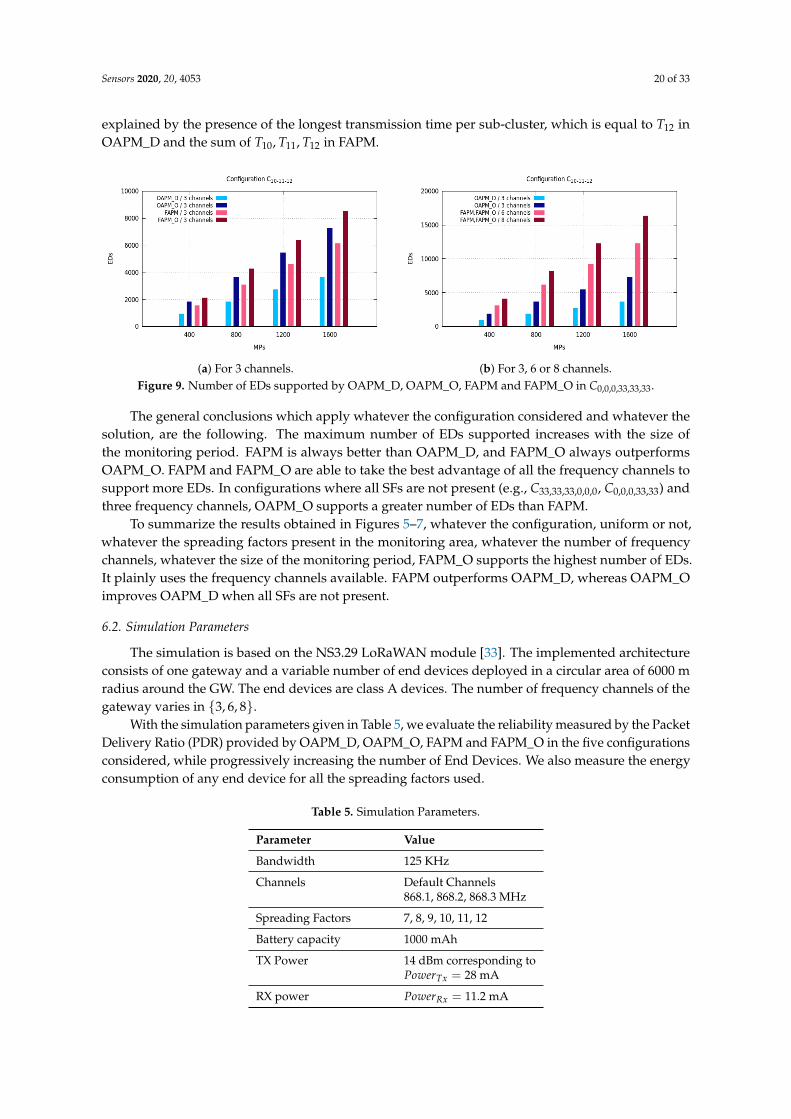
explained by the presence of the longest transmission time per sub-cluster, which is equal to T12 inOAPM_D and the sum of T10, T11, T12 in FAPM.

(a) For 3 channels. (b) For 3, 6 or 8 channels.Figure 9. Number of EDs supported by OAPM_D, OAPM_O, FAPM and FAPM_O in C0,0,0,33,33,33.

The general conclusions which apply whatever the configuration considered and whatever thesolution, are the following. The maximum number of EDs supported increases with the size ofthe monitoring period. FAPM is always better than OAPM_D, and FAPM_O always outperformsOAPM_O. FAPM and FAPM_O are able to take the best advantage of all the frequency channels tosupport more EDs. In configurations where all SFs are not present (e.g., C33,33,33,0,0,0, C0,0,0,33,33) andthree frequency channels, OAPM_O supports a greater number of EDs than FAPM.

To summarize the results obtained in Figures 5–7, whatever the configuration, uniform or not,whatever the spreading factors present in the monitoring area, whatever the number of frequencychannels, whatever the size of the monitoring period, FAPM_O supports the highest number of EDs.It plainly uses the frequency channels available. FAPM outperforms OAPM_D, whereas OAPM_Oimproves OAPM_D when all SFs are not present.

6.2. Simulation Parameters

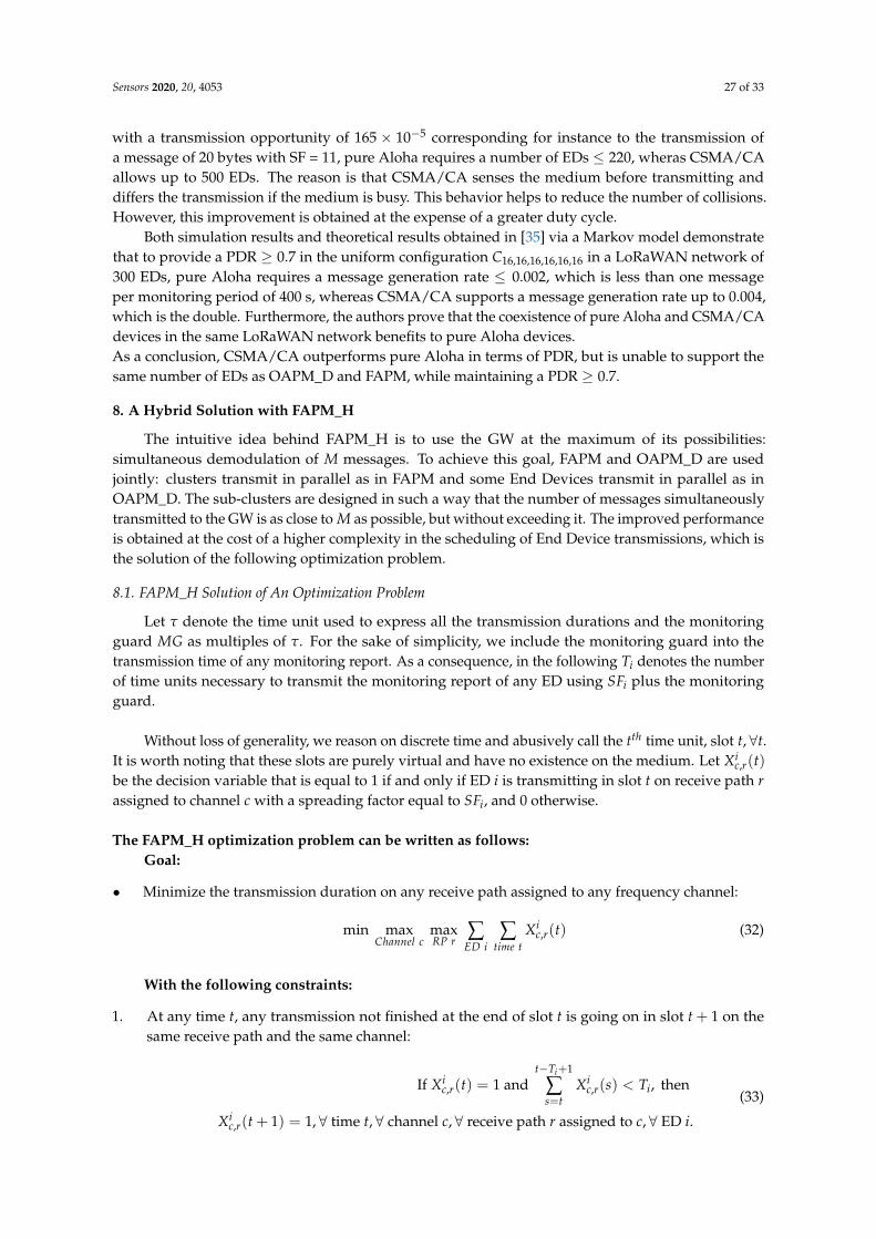
The simulation is based on the NS3.29 LoRaWAN module [33]. The implemented architectureconsists of one gateway and a variable number of end devices deployed in a circular area of 6000 mradius around the GW. The end devices are class A devices. The number of frequency channels of thegateway varies in {3, 6, 8}.

With the simulation parameters given in Table 5, we evaluate the reliability measured by the PacketDelivery Ratio (PDR) provided by OAPM_D, OAPM_O, FAPM and FAPM_O in the five configurationsconsidered, while progressively increasing the number of End Devices. We also measure the energyconsumption of any end device for all the spreading factors used.

Table 5. Simulation Parameters.

Parameter Value

Bandwidth 125 KHz

Channels Default Channels868.1, 868.2, 868.3 MHz

Spreading Factors 7, 8, 9, 10, 11, 12

Battery capacity 1000 mAh

TX Power 14 dBm corresponding toPowerTx = 28 mA

RX power PowerRx = 11.2 mA

Sensors 2020, 20, 4053 21 of 33

Table 5. Cont.

Parameter Value

Idle power PowerIdle = 1.4 mA

Sleep power PowerSleep = 15 µA

Supply Voltage 3.3 V

Number of EDs [0...5000]

Area radius 6000 m

Data payload 21 bytes

Uplink message Type Unconfirmed

Monitoring Period 400 s, 800 s, 1200 s, 1600 s

Synchronization Period 1602 s

Simulation Time 32,000 s

6.3. Packet Delivery Ratio

In this subsection, only some examples of simulation results are reported: one example perconfiguration. They are depicted in Figures 10–12 for a monitoring period equal to 400 s.

(a) in C16,16,16,16,16,16 for 6 channels. (b) in C10,20,20,20,20,10 for 6 channels.Figure 10. PDR of FAPM, OAPM_D and pure Aloha versus the number of End Devices.

(a) in C33,33,33,0,0,0 for 3 channels. (b) in C0,0,0,33,33,33 for 3 channels.Figure 11. PDR of FAPM, OAPM_D and pure Aloha versus the number of End Devices.

Sensors 2020, 20, 4053 22 of 33

Figure 12. PDR of FAPM, OAPM_D and pure Aloha in C5,15,30,35,10,5 with 3 channels versus the numberof End Devices.

We measured the PDR versus the number of EDs devices supported. Due to the hardwarelimitation, we have considered a maximum of 5000 EDs in our simulation. All curves in Figures 10–12corroborate the theoretical results presented in Sections 4.3 and 5.4. As shown in Figure 10a,b, the PDRof OAPM_D solution stabilises at 1 up to 1818 and 2020 EDs for the configurations C16,16,16,16,16,16

and C10,20,20,20,20,10, respectively, which corresponds exactly to the theoretical results given previously.Moreover, Figure 10a,b and Figure 11a show that the PDR of the FAPM solution corroborates theoreticalresults and stabilises at 1 up to 5000 EDs. In fact, ED numbers greater than 5000 have not been simulateddue to hardware limitations. And this restriction is also valid for OAPM_D results presented inFigure 11a. Simulation results illustrated in Figure 11b and Figure 12 are compliant with the theoreticalresults obtained for each solution. Pure Aloha gives the worst PDR for all the configurations evaluatedand for a much smaller number of EDs. This result shows the high efficiency of the solutions proposed.

6.4. Energy Consumption

The energy consumed by any ED during a synchronization period is the sum of:

• the energy consumed in transmitting its monitoring report once per monitoring period. Since themonitoring report message is not acknowledged and there is no retransmission, the energyconsumed for the transmission in one synchronization period is equal to the Transmission Power,PowerTx, times TRep, the transmission duration of a monitoring report using the Spreading Factorof this ED, times the number of monitoring periods in a synchronization period. This energy isthe same for all the solutions proposed.

• the energy consumed in listening to the medium, which is equal to the Idle power times thesynchronization guard SG. Again, this energy is the same for all the solutions proposed.

• the energy consumed in receiving the synchronization message, which is equal to the ReceivePower, PowerRx, times the transmission duration of the synchronization message, which is thesame for the solutions proposed.

Finally, the energy consumed by any ED per synchronization period is given by:

EnergyperSynchroPeriod = nMPperSP× TRep × PowerTx + TSync × PowerRx + SG× PowerIdle+

(SP− nMPperSP× TRep − TSync − SG)× PowerSleep.(25)

where TRep is the Transmission Time on Air of the monitoring report by this ED, and TSync theTransmission Time on Air of the synchronization message (using the maximum SF used in themonitoring area) that the ED has to receive. It is worth noting that this energy is the same forall the solutions proposed.

We evaluate by simulation the energy consumed by any ED in a synchronization period includingfour monitoring periods. Since this energy depends on the spreading factor used by the ED considered,

Sensors 2020, 20, 4053 23 of 33

six EDs are selected: one per spreading factor. Figure 13 depicts their energy consumption measuredin the simulations. These results are fully compliant with the theoretical results given by Equation (25).For any spreading factor, the energy consumption curve consists of four steps corresponding to thefour monitoring periods in the synchronization period. The horizontal part of each step highlights thealmost zero energy consumption when the ED is sleeping. It is worth noting, that EDs far fom the GWuse the highest SFs which induce a greater energy consumption.

Figure 13. ED Energy Consumption during a Synchronization period.

From Equation (25), we can deduce the lifetime of any ED battery with initial capacity Capacityas follows:

Li f etime =Capacity× Synchronization_Period

EnergyperSynchroPeriod(26)

Figure 14 depicts the lifetime of any ED equipped with a battery capacity of 1000 mAh. We noticethat the ED lifetime decreases when the spreading factor increases. The smaller lifetime of 1.13 year isobtained for SF12, whereas SF7 obtains a network lifetime of 8.83 years.

Figure 14. Network lifetime vs Spreading Factor.

The duty cycle of any ED is expressed as the percentage of time in a synchronization periodduring which the ED considered is transmitting its monitoring report or receiving the synchronizationmessage. It is given by:

Duty_cycle(ED) =TRep × nMPperSP + TSync + SG

SP(27)

Sensors 2020, 20, 4053 24 of 33

Hence, the duty cycle of any ED does not depend on the solution studied but only on itstransmit power, its receive power, its spreading factor and the spreading factor used to transmitthe synchronization message.

Table 6 gives the duty cycle of each ED according to its spreading factor for a monitoring periodof 400 s and a synchronization period of 1602 s. It is worth noting that all EDs meet the requirement ofa duty cycle ≤ 1%.

Table 6. Duty_cycle(ED) for a monitoring period of 400 s and a synchronization period of 1602 s.

Spreading Factor ED Duty_cycle (%)

SF7 0.08SF8 0.09SF9 0.11

SF10 0.15SF11 0.23SF12 0.39

7. Applicability of These Solutions

In the previous section, we have compared the scalability of OAPM_D, OAPM_O, FAPM andFAPM_O expressed by the maximum number of EDs supported. We have also evaluated the energyconsumption of each solution. In this section, we discuss the applicability of the solutions proposedwith regard to the requirements expressed by IoT applications. These constraints involve:

• the number of EDs deployed.• the geographical coordinates of each ED. The spreading factor used by the ED considered is

deduced from its distance to the GW. The cluster to which this ED belongs is computed from itsgeographical coordinates.

• the average delay between two consecutive application messages generated by the same ED,also called inter-arrival time, and the standard deviation.

• the message size.• the maximum acceptable data latency, which is defined as the maximum time elapsed between

the generation of the message including these data and its receipt by the GW.• the reliability required, which is expressed by the PDR.• the minimum lifetime of ED, which is requested by the application.• the maximum duty cycle of ED, which is accepted by the application.• the existence of an urgent traffic. If it exists, it should be described as the normal traffic is and the

reliability and latency constraints should be expressed.• the ED cost. In this paper, we assume that the ED cost is proportional to the complexity of the

solution implemented in this ED.• The coexistence with other applications sharing this GW.

7.1. Complexity

In all the solutions presented, there is no complexity in the EDs: each ED has only to transmit itsmonitoring report at the time and on the frequency channel assigned by the Network Server. All thecomplexity is left to the Network Server for the configuration of End Devices and to the GW forreceiving simultaneous messages sent by different EDs during the monitoring phase.

7.2. Data Gathering Duration

The maximum number of EDs supported by any solution presented is computed from themonitoring period to ensure collision-free transmissions of all EDs. Hence, the data gathering duration

Sensors 2020, 20, 4053 25 of 33

is very close to the Monitoring period, when the number of EDs is maximum. Notice that thismaximum depends on the solution considered.

If the number of EDs is small with regard to the maximum, the GW may support severalmonitoring applications. In such a case, the solution minimizing the data gathering duration such asFAPM_H presented in the next section, will be preferred to make the coexistence of several applicationseasier. Another advantage of a solution minimizing the data gathering duration is to ensure a bettertime consistency of all the samples collected since they have been collected at closer times.

7.3. Data Latency

Since in all the solutions proposed, the transmission of the monitoring report produced by eachED is scheduled, the generation of a new message corresponding to a new measure is not immediatelyfollowed by its transmission, some latency may exist.

In the worst case, the new message is generated just after the ED considered starts the transmissionof its monitoring report. Consequently, the new message will be transmitted in the next monitoringperiod. In the worst case, this next monitoring period is preceded by a synchronization. The maximumlatency is equal to:

MaxLatency = MP + TSync + 2SG + TRep, (28)

where TRep denotes the Time on Air of the monitoring report transmitted by this ED, TSync is the Timeon Air of the synchronization message transmitted with the highest SF in the configuration.

Since a new message may be generated at any time in the monitoring period and the nextmonitoring period is preceded by a synchronization once per nMPperSP, the average latency is equalto:

AverageLatency =MP

2+

TSync + 2SG2nMPperSP

+ TRep. (29)

7.4. Urgent Traffic Support

Some monitoring IoT applications support two classes of traffic: urgent and normal. Urgent trafficshould be delivered promptly to the GW. If the requirements for normal traffic are fully compliant withthe average latency and the maximum latency given by Equation (29) and by Equation (28), respectively,it is usually not the case for the urgent traffic. The solutions proposed can easily be extended byassuming that only a small number of EDs can generate urgent messages (Assumption A15). TheseEDs, denoted Urg_EDs, maintain two buffers: one for an urgent message and one for a normalmessage, whereas the remaining EDs, denoted Norm_EDs, maintain only one buffer for a normalmessage. The monitoring period is subdivided into a multiple of urgent monitoring periods. In eachurgent monitoring period, there are three parts:

• The first one is left to Urg_EDs. They are the only devices allowed to transmit in this part.They transmit an urgent message, if it exists, and a normal message otherwise. As a consequence,an Urg_ED has as many opportunities to transmit urgent messages as the number of urgentmonitoring periods in a monitoring period.

• The second part is left to some Norm_EDs. Norm_EDs are assigned to urgent monitoring periodsin such a way that each Norm_ED has a single opportunity to transmit in each monitoring period.

• This third part may be empty, it depends on the application requirements. In the third part,all devices are sleeping to save energy.

With Assumption A15, the maximum latency of urgent traffic is given by:

MaxUrgentLatency = UMP + TSync + 2SG + TUrg, (30)

Sensors 2020, 20, 4053 26 of 33

where UMP is the Urgent Monitoring Period, TUrg denotes the Time on Air of the urgent messagetransmitted by this ED.

With Assumption A15, the average latency of urgent traffic is equal to:

AverageUrgentLatency =UMP

2+

TSync + 2SGnMPperSP

+ TUrg. (31)

If Assumption A15 is not met, the monitoring period becomes very close to the urgent monitoringperiod and the number of EDs supported decreases to meet the latency of urgent messages. If onerequirement of the IoT application is not met, the solution cannot be applied.

7.5. Probabilistic Traffic

Up to now we have only considered the case where each ED generates a single message in eachmonitoring period. We now take into account the fact any ED may generate 0, 1 or more messagesper monitoring period. Traffic generation is now probabilistic. For simplicity reasons, the size of thebuffer of each ED is set to one monitoring message. When a new message is generated, it replacesthe previous one. This is consistent with the data freshness required by the monitoring applications.As a consequence, a given monitoring message may be never transmitted if a new message has alreadyreplaced it.

We now consider probabilistic traffic. Each ED generates a Poisson traffic with inter-arrival timeequal to the monitoring period MP = 400 s. We consider the uniform configuration with six channelsand compare the performances of the solutions studied in terms of reliability in Figure 15a and latencyof the messages delivered to the GW in Figure 15b, respectively. The number of EDs for each solutionevaluated is equal to 1812, except for Aloha where it is equal to 400. With regard to latency, simulationresults corroborate the theoretical results. With regard to reliability, simulation results provide therates of (i) messages overwritten (i.e., denoted lost in Figure 15a), and messages received over the totalnumber of messages generated, and (ii) messages delivered among those transmitted, which is thePDR. It appears that the main reason for unreliability is due to the overwriting of messages in the caseof a buffer of size one message. To reduce these losses, a smaller monitoring period could be used.All the solutions proposed ensure a PDR equal to one, whereas pure Aloha with a smaller numberof EDs (i.e., less than the quarter of the number of EDs used for the other solutions) ensures a PDRequal to 0.7. This shows the efficiency of the solutions proposed. Figure 15b shows an average latencyaround 222 s for all the solutions evaluated, in accordance with Equation (29).

(a) Comparative reliability. (b) Comparative latency.Figure 15. Comparative performance evaluation of pure Aloha, OAPM_D and FAPM in C16,16,16,16,16,16.

CSMA/CA and pure Aloha have been well analyzed and evaluated in the literature.However their performances have been compared considering saturated traffic on all devices. Thisassumption is no longer valid for IoT monitoring applications. In addition, the metric evaluated was thenetwork throughput, whereas in IoT monitoring applications, metrics such as PDR, latency and energyconsumption are more relevant. In [34], the authors show by simulation that to ensure a PDR ≥ 0.7

Sensors 2020, 20, 4053 27 of 33

with a transmission opportunity of 165 × 10−5 corresponding for instance to the transmission ofa message of 20 bytes with SF = 11, pure Aloha requires a number of EDs ≤ 220, wheras CSMA/CAallows up to 500 EDs. The reason is that CSMA/CA senses the medium before transmitting anddiffers the transmission if the medium is busy. This behavior helps to reduce the number of collisions.However, this improvement is obtained at the expense of a greater duty cycle.

Both simulation results and theoretical results obtained in [35] via a Markov model demonstratethat to provide a PDR ≥ 0.7 in the uniform configuration C16,16,16,16,16,16 in a LoRaWAN network of300 EDs, pure Aloha requires a message generation rate ≤ 0.002, which is less than one messageper monitoring period of 400 s, whereas CSMA/CA supports a message generation rate up to 0.004,which is the double. Furthermore, the authors prove that the coexistence of pure Aloha and CSMA/CAdevices in the same LoRaWAN network benefits to pure Aloha devices.As a conclusion, CSMA/CA outperforms pure Aloha in terms of PDR, but is unable to support thesame number of EDs as OAPM_D and FAPM, while maintaining a PDR ≥ 0.7.

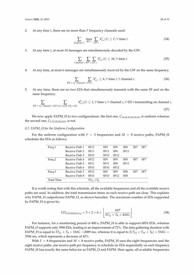
8. A Hybrid Solution with FAPM_H

The intuitive idea behind FAPM_H is to use the GW at the maximum of its possibilities:simultaneous demodulation of M messages. To achieve this goal, FAPM and OAPM_D are usedjointly: clusters transmit in parallel as in FAPM and some End Devices transmit in parallel as inOAPM_D. The sub-clusters are designed in such a way that the number of messages simultaneouslytransmitted to the GW is as close to M as possible, but without exceeding it. The improved performanceis obtained at the cost of a higher complexity in the scheduling of End Device transmissions, which isthe solution of the following optimization problem.

8.1. FAPM_H Solution of An Optimization Problem

Let τ denote the time unit used to express all the transmission durations and the monitoringguard MG as multiples of τ. For the sake of simplicity, we include the monitoring guard into thetransmission time of any monitoring report. As a consequence, in the following Ti denotes the numberof time units necessary to transmit the monitoring report of any ED using SFi plus the monitoringguard.

Without loss of generality, we reason on discrete time and abusively call the tth time unit, slot t, ∀t.It is worth noting that these slots are purely virtual and have no existence on the medium. Let Xi

c,r(t)be the decision variable that is equal to 1 if and only if ED i is transmitting in slot t on receive path rassigned to channel c with a spreading factor equal to SFi, and 0 otherwise.

The FAPM_H optimization problem can be written as follows:Goal:

• Minimize the transmission duration on any receive path assigned to any frequency channel:

min maxChannel c

maxRP r

∑ED i

∑time t

Xic,r(t) (32)

With the following constraints:

1. At any time t, any transmission not finished at the end of slot t is going on in slot t + 1 on thesame receive path and the same channel:

If Xic,r(t) = 1 and

t−Ti+1

∑s=t

Xic,r(s) < Ti, then

Xic,r(t + 1) = 1, ∀ time t, ∀ channel c, ∀ receive path r assigned to c, ∀ ED i.

(33)

Sensors 2020, 20, 4053 28 of 33

2. At any time t, there are no more than F frequency channels used:

∑Channel c

maxRP r

∑ED i

Xic,r(t) ≤ F, ∀ time t. (34)

3. At any time t, at most M messages are simultaneously decoded by the GW:

∑Channel c

∑RP r

∑ED i

Xic,r(t) ≤ M, ∀ time t. (35)

4. At any time, at most 6 messages are simultaneously received by the GW on the same frequency.

∑RP r o f channel c

∑ED i

Xic,r ≤ 6, ∀ time t, ∀ channel c. (36)

5. At any time, there are no two EDs that simultaneously transmit with the same SF and on thesame frequency:

∑RP r o f channel c

∑ED k 6=i with SFk=SFi

Xkc,r(t) ≤ 1, ∀ time t, ∀ channel c, ∀ ED i transmitting on channel c.

(37)

We now apply FAPM_H to two configurations: the first one, C16,16,16,16,16,16, is uniform whereasthe second one, C5,15,35,30,10,5, is not.

8.2. FAPM_H for the Uniform Configuration

For the uniform configuration with F = 3 frequencies and M = 8 receive paths, FAPM_Hschedules the EDs as follows:

Freq 1 Receive Path 1 SF12 SF9 SF9 SF8 SF7 SF7Receive Path 2 SF11 SF11 SF8 SF11Receive Path 3 SF10 SF10 SF12

Freq 2 Receive Path 4 SF12 SF9 SF9 SF8 SF7 SF7Receive Path 5 SF11 SF11 SF8 SF11Receive Path 6 SF10 SF10 SF12

Freq 3 Receive Path 7 SF12 SF9 SF9 SF8 SF7 SF7Receive Path 8 SF10 SF10 SF12 SF8

Total Time 3T11 +T8

It is worth noting that with this schedule, all the available frequencies and all the available receivepaths are used. In addition, the total transmission times on each receive path are close. This explainswhy FAPM_H outperforms FAPM_O, as shown hereafter: The maximum number of EDs supportedby FAPM_H is given by:

EDFAPMH3 f req = 3× 2× 6×⌊

MP3T11 + T8 + 4MG

⌋. (38)

For instance, for a monitoring period of 400 s, FAPM_H is able to support 6876 EDs, whereasFAPM_O supports only 3996 EDs, leading to an improvement of 72%. The data gathering duration withFAPM_H is equal to 3T11 + T8 + 3MG =2089 ms, whereas it is equal to 2(T12 + T10 + T8) + 5MG =

3596 ms, which represents a decrease of 42%.With F = 8 frequencies and M = 8 receive paths, FAPM_H uses the eight frequencies and the

eight receive paths, one receive path per frequency, to schedule six EDs sequentially on each frequency.FAPM_H has exactly the same behavior as FAPM_O and FAPM. Here again, all available frequencies

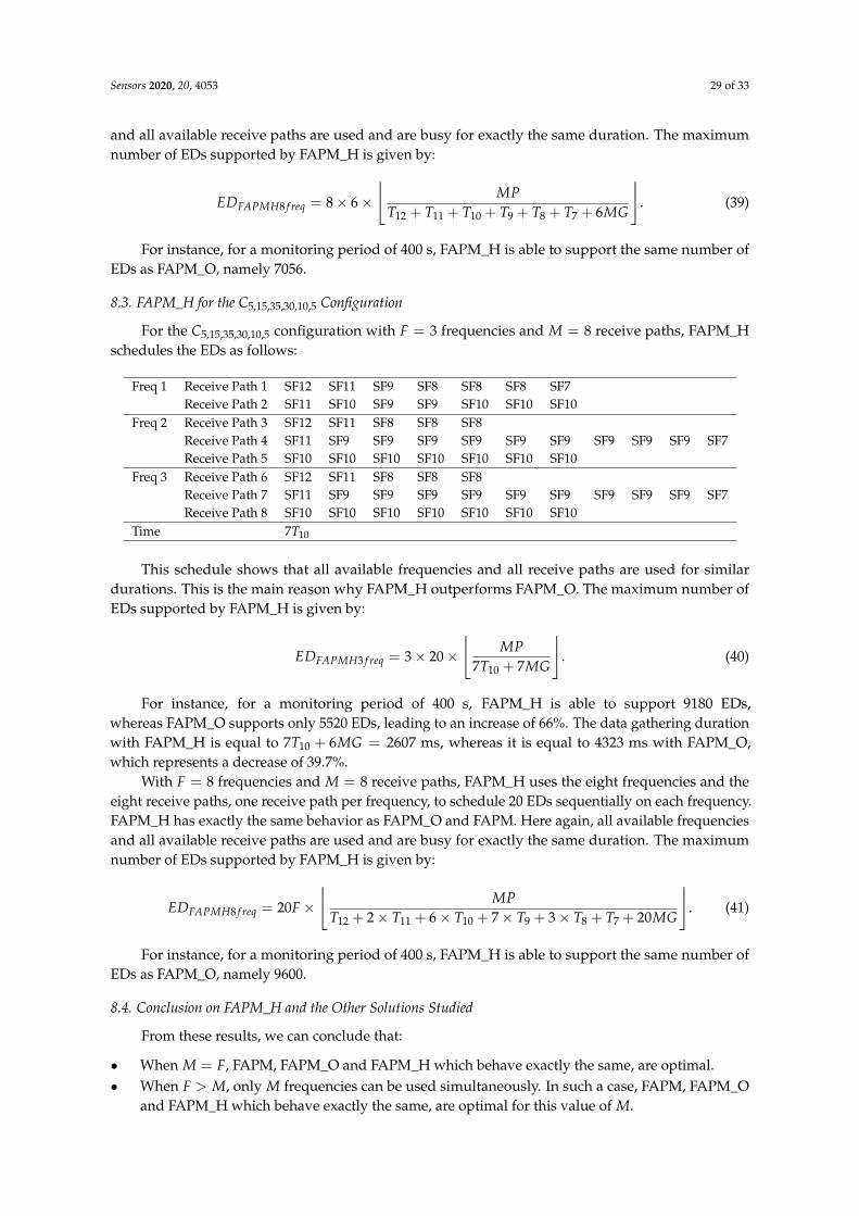
Sensors 2020, 20, 4053 29 of 33

and all available receive paths are used and are busy for exactly the same duration. The maximumnumber of EDs supported by FAPM_H is given by:

EDFAPMH8 f req = 8× 6×⌊

MPT12 + T11 + T10 + T9 + T8 + T7 + 6MG

⌋. (39)

For instance, for a monitoring period of 400 s, FAPM_H is able to support the same number ofEDs as FAPM_O, namely 7056.

8.3. FAPM_H for the C5,15,35,30,10,5 Configuration

For the C5,15,35,30,10,5 configuration with F = 3 frequencies and M = 8 receive paths, FAPM_Hschedules the EDs as follows:

Freq 1 Receive Path 1 SF12 SF11 SF9 SF8 SF8 SF8 SF7Receive Path 2 SF11 SF10 SF9 SF9 SF10 SF10 SF10

Freq 2 Receive Path 3 SF12 SF11 SF8 SF8 SF8Receive Path 4 SF11 SF9 SF9 SF9 SF9 SF9 SF9 SF9 SF9 SF9 SF7Receive Path 5 SF10 SF10 SF10 SF10 SF10 SF10 SF10

Freq 3 Receive Path 6 SF12 SF11 SF8 SF8 SF8Receive Path 7 SF11 SF9 SF9 SF9 SF9 SF9 SF9 SF9 SF9 SF9 SF7Receive Path 8 SF10 SF10 SF10 SF10 SF10 SF10 SF10

Time 7T10

This schedule shows that all available frequencies and all receive paths are used for similardurations. This is the main reason why FAPM_H outperforms FAPM_O. The maximum number ofEDs supported by FAPM_H is given by:

EDFAPMH3 f req = 3× 20×⌊

MP7T10 + 7MG

⌋. (40)

For instance, for a monitoring period of 400 s, FAPM_H is able to support 9180 EDs,whereas FAPM_O supports only 5520 EDs, leading to an increase of 66%. The data gathering durationwith FAPM_H is equal to 7T10 + 6MG = 2607 ms, whereas it is equal to 4323 ms with FAPM_O,which represents a decrease of 39.7%.

With F = 8 frequencies and M = 8 receive paths, FAPM_H uses the eight frequencies and theeight receive paths, one receive path per frequency, to schedule 20 EDs sequentially on each frequency.FAPM_H has exactly the same behavior as FAPM_O and FAPM. Here again, all available frequenciesand all available receive paths are used and are busy for exactly the same duration. The maximumnumber of EDs supported by FAPM_H is given by:

EDFAPMH8 f req = 20F×⌊

MPT12 + 2× T11 + 6× T10 + 7× T9 + 3× T8 + T7 + 20MG

⌋. (41)

For instance, for a monitoring period of 400 s, FAPM_H is able to support the same number ofEDs as FAPM_O, namely 9600.

8.4. Conclusion on FAPM_H and the Other Solutions Studied

From these results, we can conclude that:

• When M = F, FAPM, FAPM_O and FAPM_H which behave exactly the same, are optimal.• When F > M, only M frequencies can be used simultaneously. In such a case, FAPM, FAPM_O

and FAPM_H which behave exactly the same, are optimal for this value of M.

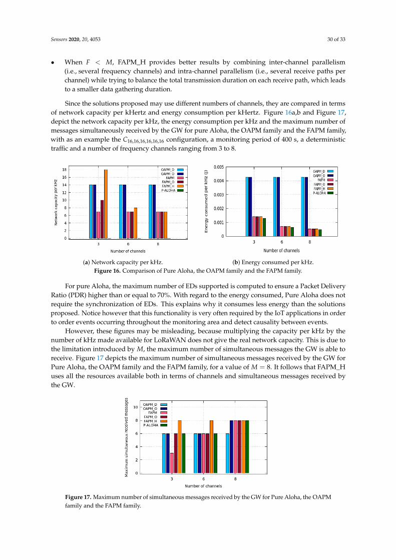
Sensors 2020, 20, 4053 30 of 33

• When F < M, FAPM_H provides better results by combining inter-channel parallelism(i.e., several frequency channels) and intra-channel parallelism (i.e., several receive paths perchannel) while trying to balance the total transmission duration on each receive path, which leadsto a smaller data gathering duration.

Since the solutions proposed may use different numbers of channels, they are compared in termsof network capacity per kHertz and energy consumption per kHertz. Figure 16a,b and Figure 17,depict the network capacity per kHz, the energy consumption per kHz and the maximum number ofmessages simultaneously received by the GW for pure Aloha, the OAPM family and the FAPM family,with as an example the C16,16,16,16,16,16 configuration, a monitoring period of 400 s, a deterministictraffic and a number of frequency channels ranging from 3 to 8.

(a) Network capacity per kHz. (b) Energy consumed per kHz.Figure 16. Comparison of Pure Aloha, the OAPM family and the FAPM family.

For pure Aloha, the maximum number of EDs supported is computed to ensure a Packet DeliveryRatio (PDR) higher than or equal to 70%. With regard to the energy consumed, Pure Aloha does notrequire the synchronization of EDs. This explains why it consumes less energy than the solutionsproposed. Notice however that this functionality is very often required by the IoT applications in orderto order events occurring throughout the monitoring area and detect causality between events.

However, these figures may be misleading, because multiplying the capacity per kHz by thenumber of kHz made available for LoRaWAN does not give the real network capacity. This is due tothe limitation introduced by M, the maximum number of simultaneous messages the GW is able toreceive. Figure 17 depicts the maximum number of simultaneous messages received by the GW forPure Aloha, the OAPM family and the FAPM family, for a value of M = 8. It follows that FAPM_Huses all the resources available both in terms of channels and simultaneous messages received bythe GW.

Figure 17. Maximum number of simultaneous messages received by the GW for Pure Aloha, the OAPMfamily and the FAPM family.

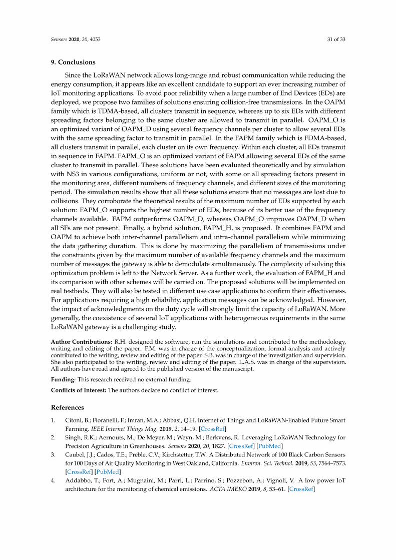
Sensors 2020, 20, 4053 31 of 33

9. Conclusions

Since the LoRaWAN network allows long-range and robust communication while reducing theenergy consumption, it appears like an excellent candidate to support an ever increasing number ofIoT monitoring applications. To avoid poor reliability when a large number of End Devices (EDs) aredeployed, we propose two families of solutions ensuring collision-free transmissions. In the OAPMfamily which is TDMA-based, all clusters transmit in sequence, whereas up to six EDs with differentspreading factors belonging to the same cluster are allowed to transmit in parallel. OAPM_O isan optimized variant of OAPM_D using several frequency channels per cluster to allow several EDswith the same spreading factor to transmit in parallel. In the FAPM family which is FDMA-based,all clusters transmit in parallel, each cluster on its own frequency. Within each cluster, all EDs transmitin sequence in FAPM. FAPM_O is an optimized variant of FAPM allowing several EDs of the samecluster to transmit in parallel. These solutions have been evaluated theoretically and by simulationwith NS3 in various configurations, uniform or not, with some or all spreading factors present inthe monitoring area, different numbers of frequency channels, and different sizes of the monitoringperiod. The simulation results show that all these solutions ensure that no messages are lost due tocollisions. They corroborate the theoretical results of the maximum number of EDs supported by eachsolution: FAPM_O supports the highest number of EDs, because of its better use of the frequencychannels available. FAPM outperforms OAPM_D, whereas OAPM_O improves OAPM_D whenall SFs are not present. Finally, a hybrid solution, FAPM_H, is proposed. It combines FAPM andOAPM to achieve both inter-channel parallelism and intra-channel parallelism while minimizingthe data gathering duration. This is done by maximizing the parallelism of transmissions underthe constraints given by the maximum number of available frequency channels and the maximumnumber of messages the gateway is able to demodulate simultaneously. The complexity of solving thisoptimization problem is left to the Network Server. As a further work, the evaluation of FAPM_H andits comparison with other schemes will be carried on. The proposed solutions will be implemented onreal testbeds. They will also be tested in different use case applications to confirm their effectiveness.For applications requiring a high reliability, application messages can be acknowledged. However,the impact of acknowledgments on the duty cycle will strongly limit the capacity of LoRaWAN. Moregenerally, the coexistence of several IoT applications with heterogeneous requirements in the sameLoRaWAN gateway is a challenging study.

Author Contributions: R.H. designed the software, run the simulations and contributed to the methodology,writing and editing of the paper. P.M. was in charge of the conceptualization, formal analysis and activelycontributed to the writing, review and editing of the paper. S.B. was in charge of the investigation and supervision.She also participated to the writing, review and editing of the paper. L.A.S. was in charge of the supervision.All authors have read and agreed to the published version of the manuscript.

Funding: This research received no external funding.

Conflicts of Interest: The authors declare no conflict of interest.

References

1. Citoni, B.; Fioranelli, F.; Imran, M.A.; Abbasi, Q.H. Internet of Things and LoRaWAN-Enabled Future SmartFarming. IEEE Internet Things Mag. 2019, 2, 14–19. [CrossRef]

2. Singh, R.K.; Aernouts, M.; De Meyer, M.; Weyn, M.; Berkvens, R. Leveraging LoRaWAN Technology forPrecision Agriculture in Greenhouses. Sensors 2020, 20, 1827. [CrossRef] [PubMed]

3. Caubel, J.J.; Cados, T.E.; Preble, C.V.; Kirchstetter, T.W. A Distributed Network of 100 Black Carbon Sensorsfor 100 Days of Air Quality Monitoring in West Oakland, California. Environ. Sci. Technol. 2019, 53, 7564–7573.[CrossRef] [PubMed]

4. Addabbo, T.; Fort, A.; Mugnaini, M.; Parri, L.; Parrino, S.; Pozzebon, A.; Vignoli, V. A low power IoTarchitecture for the monitoring of chemical emissions. ACTA IMEKO 2019, 8, 53–61. [CrossRef]

Sensors 2020, 20, 4053 32 of 33

5. Yu, F.; Zhu, Z.; Fan, Z. Study on the feasibility of LoRaWAN for smart city applications. In Proceedingsof the 2017 IEEE 13th International Conference on Wireless and Mobile Computing, Networking andCommunications (WiMob), Rome, Italy, 9–11 October 2017; pp. 334–340.

6. Semtech, Wireless and Sensing Products Datasheet. Available online: https://www.semtech.com/products/wireless-rf/lora-gateways/sx1301#download-resources (accessed on 5 May 2020).

7. Queralta, J.; Gia, T.; Zou, Z.; Tenhunen, H.; Westerlund, T. Comparative study of LPWAN technologies onunlicensed bands for M2M communication in the IoT: beyond LoRa and LoRaWAN. Procedia Comput. Sci.2019, 155, 343–350. [CrossRef]

8. Zorbas, D.; Abdelfadeel, K.; Kotzanikolaou, P.; Pesch, D. TS-LoRa: Time-slotted LoRaWAN for the IndustrialInternet of Things. Comput. Commun. 2020, 153, 1–10. [CrossRef]

9. Haxhibeqiri, J.; Moerman, I.; Hoebeke, J. Low overhead scheduling of lora transmissions for improvedscalability. IEEE Internet Things J. 2018, 6, 3097–3109. [CrossRef]

10. Polonelli, T.; Brunelli, D.; Marzocchi, A.; Benini, L. Slotted aloha on lorawan-design, analysis, anddeployment. Sensors 2019, 19, 838. [CrossRef] [PubMed]

11. Adelantado, F.; Vilajosana, X.; Tuset-Peiro, P.; Martinez, B.; Melia-Segui, J.; Watteyne, T. Understanding theLimits of LoRaWAN. IEEE Commun. Mag. 2017, 55, 34–40. [CrossRef]

12. Bor, M.C.; Roedig, U.; Voigt, T.; Alonso, J.M. Do LoRa Low-Power Wide-Area Networks Scale?In Proceedings of the 19th ACM International Conference on Modeling, Analysis and Simulation of Wirelessand Mobile Systems (MSWIM), Malta, Malta, 13–17 November 2016; pp. 59–67.

13. LoRa Alliance. LoRaWAN 1.0.3 Specification. Available online: https://lora-alliance.org/resource-hub/lorawanr-specification-v103 (accessed on 25 January 2020).

14. Davcev, D.; Mitreski, K.; Trajkovic, S.; Nikolovski, V.; Koteli, N. IoT agriculture system based on LoRaWAN.In Proceedings of the 2018 14th IEEE International Workshop on Factory Communication Systems (WFCS),Imperia, Italy, 13–15 June 2018; pp. 1–4.

15. Basford, P.J.; Bulot, F.M.; Apetroaie-Cristea, M.; Cox, S.J.; Ossont, S.J. LoRaWAN for smart city IoTdeployments: A long term evaluation. Sensors 2020, 20, 648. [CrossRef] [PubMed]

16. Johnston, S.J.; Basford, P.J.; Bulot, F.M.; Apetroaie-Cristea, M.; Easton, N.H.; Davenport, C.; Foster, G.L.;Loxham, M.; Morris, A.K.; Cox, S.J. City scale particulate matter monitoring using LoRaWAN based airquality IoT devices. Sensors 2019, 19, 209. [CrossRef] [PubMed]

17. LoRa Alliance. What is LoRaWAN: A Technical Overview of LoRa and LoRaWAN. Available online:https://lora-alliance.org/resource-hub/what-lorawanrJan (accessed on 25 January 2020).

18. CEPT, Electronic Communications Committee. ERC Recommendation 70-03. Available online: https://www.ecodocdb.dk/download/25c41779-cd6e/Rec7003e.pdf (accessed on 15 July 2020).

19. Goursaud, C.; Gorce, J.M. Dedicated networks for IoT: PHY/MAC state of the art and challenges.EAI Endorsed Trans. Internet Things 2015. [CrossRef]

20. Capuzzo, M.; Magrin, D.; Zanella, A. Confirmed traffic in LoRaWAN: Pitfalls and countermeasures.In Proceedings of the 2018 17th Annual Mediterranean Ad Hoc Networking Workshop (Med-Hoc-Net),Capri, Italy, 20–22 June 2018; pp.1–7. [CrossRef]

21. Iova, O.; Murphy, A.; Picco, G.P.; Ghiro, L.; Molteni, D.; Ossi, F.; Cagnacci, F. LoRa from the city to themountains: Exploration of hardware and environmental factors. In Proceedings of the 2017 InternationalConference on Embedded Wireless Systems and Networks, Uppsala, Sweden, 20–22 February 2017.

22. Petajajarvi, J.; Mikhaylov, K.; Roivainen, A.; Hanninen, T.; Pettissalo, M. On the coverage of LPWANs:Range evaluation and channel attenuation model for LoRa technology. In Proceedings of the 2015 14thInternational Conference on ITS Telecommunications (ITST), Copenhagen, Denmark, 2–4 December 2015;pp. 55–59.

23. Bankov, D.; Khorov, E.; Lyakhov, A. On the limits of LoRaWAN channel access. In Proceedings ofthe 2016 International Conference on Engineering and Telecommunication (EnT), Dolgoprudny, Russia,29–30 November 2016; pp. 10–14.

24. Eletreby, R.; Zhang, D.; Kumar, S.; Yagan, O. Empowering low-power wide area networks in urban settings.In Proceedings of the Conference of the ACM Special Interest Group on Data Communication (SIGCOM),Los Angeles, CA, USA, 21–25 August 2017; pp. 309–321.

Sensors 2020, 20, 4053 33 of 33

25. Gadre, A.; Yi, F.; Rowe, A.; Iannucci, B.; Kumar, S. Quick (and Dirty) Aggregate Queries on Low-PowerWANs. In Proceedings of the 2020 The 19th ACM/IEEE Conference on Information Processing in SensorNetworks (IPSN), Sydney, Australia, 21–24 April 2020.

26. Dongare, A.; Narayanan, R.; Gadre, A.; Luong, A.; Balanuta, A.; Kumar, S.; Iannucci, B.; Rowe, A.Charm: Exploiting geographical diversity through coherent combining in low-power wide-area networks.In Proceedings of the 2018 17th ACM/IEEE International Conference on Information Processing in SensorNetworks (IPSN), Porto, Portugal, 11–13 April 2018; pp. 60–71.

27. Polonelli, T.; Brunelli, D.; Benini, L. Slotted aloha overlay on lorawan-a distributed synchronization approach.In Proceedings of the 2018 IEEE 16th International Conference on Embedded and Ubiquitous Computing(EUC), Bucharest, Romania, 29–31 October 2018; pp. 129–132.

28. Ramirez, C.G.; Sergeyev, A.; Dyussenova, A.; Iannucci, B. LongShoT: Long-range synchronization of time.In Proceedings of the 18th International Conference on Information Processing in Sensor Networks (IPSN),Montreal, QC, Canada, 16–18 April 2019; pp. 289–300.

29. Gao, S.; Zhang, X.; Du, C.; Ji, Q. A Multichannel Low-Power Wide-Area Network With High-AccuracySynchronization Ability for Machine Vibration Monitoring. IEEE Internet Things J. 2019, 6, 5040–5047.[CrossRef]

30. World Health Organization. Ambient Air Pollution: A Global Assessment of Exposure and Burden of Disease;World Health Organization: Geneva, Switzerland, 2016.

31. US Environmental Protection Agency and US Environmental Protection Agency, Office of Air QualityPlanning and Standards, Outreach and Information Division. Air Quality Index: A Guide to Air Qualityand Your Health. EPA-456/F-14-002. Research Triangle Park, NC: 2014. Available online: https://www.airnow.gov/air-quality-index-publications/ (accessed on 25 January 2020).

32. Rizzi, M.; Depari, A.; Ferrari, P.; Flammini, A.; Rinaldi, S.; Sisinni, E. Synchronization Uncertainty VersusPower Efficiency in LoRaWAN Networks. IEEE Trans. Instrum. Meas. 2019, 68, 1101–1111. [CrossRef]

33. Magrin, D.; Centenaro, M.; Vangelista, L. Performance evaluation of LoRa networks in a smart cityscenario. In Proceedings of the 2017 IEEE International Conference on Communications (ICC), Paris, France,21–25 May 2017; pp. 1–7.

34. Ben Khalifa, A.; Stanica, R. Performance Evaluation of Channel Access Methods for Dedicated IoT Networks.In Proceedings of the 2019 Wireless Days (WD), Manchester, UK, 24–26 April 2019.

35. Ortín, J.; Cesana, M.; Redondi, A. How do ALOHA and Listen Before Talk Coexist in LoRaWAN?In Proceedings of the 2018 IEEE 29th Annual International Symposium on Personal, Indoor and MobileRadio Communications (PIMRC), Bologna, Italy, 9–12 September 2018.

c© 2020 by the authors. Licensee MDPI, Basel, Switzerland. This article is an open accessarticle distributed under the terms and conditions of the Creative Commons Attribution(CC BY) license (http://creativecommons.org/licenses/by/4.0/).