Copyright © 2010, 2012 by Aldo Musacchio, André Martínez Fritscher, and Martina Viarengo

Working papers are in draft form. This working paper is distributed for purposes of comment and discussion only. It may not be reproduced without permission of the copyright holder. Copies of working papers are available from the author.

Colonial Institutions, Trade Shocks, and the Diffusion of Elementary Education in Brazil, 1889-1930 Aldo Musacchio André Martínez Fritscher Martina Viarengo

Working Paper

10-075 December 18, 2012

Colonial Institutions, Trade Shocks, and the Diffusion of Elementary Education in Brazil,

1889-1930

Aldo Musacchio* Harvard Business School and NBER

André Martínez Fritscher

Banco de Mexico

Martina Viarengo The Graduate Institute, Geneva

Abstract

In this paper, we examine the role of trade shocks in promoting the diffusion of elementary education in subnational units in Brazil during a period (1889-1930) in which they had relative financial autonomy to collect export taxes and spend on public goods. The argument is that trade shocks affect asymetrically the tax revenues of state governments and, thus, their expenditures on elementary education per capita according to what crop mix they had. We then show that states with more egalitarian and democratic institutions use positive trade shocks to invest in education, while the opposite takes place in states with less democratic institutions (e.g., in states that had more slaves). We also show using OLS and instrumental variables that positive trade shocks increased expenditures on education per capita and led to higher literacy rates and to more schools per children. The resulting distribution of human capital across states persists until today.

This version: December, 2012

* Musacchio is the corresponding author, amusacchio@hbs.edu, Harvard Business School, Morgan Hall 279, Boston, MA 02163. Research assistance for this paper was ably provided by Jenna Bernhardson and Carlos L. Góes. We benefited from comments to earlier drafts by Ran Abramitsky, Dan Bogart, Carlos Capistrán, Eric Chaney, Karen Clay, Rafel DiTella, Catherine Duggan, Stan Engerman, Felipe T. Fernandes, Cláudio Ferraz, Mary Hansen, Eric Hilt, Richard Hornbeck, Lakshmi Iyer, Joseph L. Love, Ricardo Madeira, Noel Maurer, João Manuel P. de Mello, David Moss, Joana Naritomi, Tom Nicholas, Robert Margo, Steve Nafziger, Nathan Nunn, Ian Read, Eustáquio Reis, Rodrigo Soares, Peter Temin, John Wallis, Jeff Williamson and participants in seminars at Harvard University, Harvard Business School, Stanford University, UC Berkeley, UC Davies, PUC and FGV in Rio, USP, and CIDE and Banco de México in Mexico City. We also thank commentators and participants at the ASSA, EHA, Cliometrics and CLADE-II conferences. The usual caveats apply.

1

Introduction

Recent research links the inequality we observe today across former colonies, and even

within regions in former colonies, to colonial institutions.1 According to this literature,

endowments and the conditions at the time of colonization determined a set of political

institutions that ended up perpetuating an unequal distribution of land, wealth, and political

power. In fact, the variation in colonial institutions has been identified as a cause of

heterogeneity in expenditures on public goods per capita, such as education, both across

countries or within countries.2 In general, the causal argument of this literature is that because

colonial institutions were determined hundreds of years ago, finding correlations with today’s

economic outcomes shows causality from the former to the latter.

Yet, finding correlations between variables that were observed hundreds of years apart

begs further examination. Do colonial institutions determine outcomes that then persist for

hundreds of years or do they matter only after economies suffer specific shocks that make those

institutions binding? Could it be the case that these correlations are proxies for something else

that may explain today’s outcomes? So far we only have scant evidence of how much colonial

institutions led to monotonic trends in economic development and about how institutions,

inequality, and economic outcomes change over time in former colonies. For instance, we know

that in the nineteenth century former colonies in what is now Latin America experienced a

radical reversal of fortune for the worse. We also know that there have been significant

reversals in legal institutions and financial development across countries in the twentieth

century. Finally, there is also evidence that trade shocks in the nineteenth century increased

inequality within countries in the Americas.3

In this paper we identify heterogeneous trade shocks between 1890 and 1930 that were

translated into significant differences in revenues and expenditures on education per capita

among state governments in Brazil. Those shocks explain why some states were able to spend

1 Acemoglu, Johnson, and Robinson, “Colonial Origins;” Engerman and Sokoloff, “Factor Endowments” and “History Lessons;” Nunn, “ Slavery;” and Bruhn and Gallego, “Good, Bad, and Ugly.”

2 For studies explaining variation in expenditures on education see Engerman, Mariscal, and Sokoloff, “Evolution of Schooling” and Gallego, “Historical Origins. For studies looking at variation in education expenditures within countries see Banerjee and Iyer, “History;” Iyer, “Direct versus Indirect;” and, Wegenast, “Cana, Café, Cacau” and “Legacy of Landlords.”

3 For reversals of fortune see Acemoglu, Johnson, and Robinson, “Reversal of Fortune;” Coatsworth,”Structures” and “Inequality.” Reversals of financial development are documented in Rajan and Zingales, “Great Reversals” and Musacchio, “Can Civil Law.” For the relationship between trade shocks and inequality see Williamson “History without Evidence” and Arroyo-Abad, “Persistent Inequality?”

2

more and lead in the diffusion of elementary education in Brazil, while others lagged behind.

We argue that trade shocks made political institutions binding, as the shocks to government

revenues were attenuated by the type how much of the positive trade shocks turned into

expenditure on education.

By focusing on variation over time, rather than just on path dependence since colonial

times, our findings contribute to the growing literature on the long-term effects of colonial

institutions in Brazil. In particular, our paper adds a time dimension to a relatively “time-less”

literature. In Brazil, studies of the long term effects of the so-called colonial institutions have

proliferated. Naritomi, Soares and Assunção, find significant correlations in municipalities with

extractive institutions during colonial times, (i.e., mining and sugar areas), and municipalities

that today have worse indicators of rule of law and legal sophistication. Wegenast in a cross-

sectional framework shows that land inequality is correlated with educational attainment at the

state level. Since land inequality was mostly determined during colonial times, this author

argues there is causality from land inequality to education levels. In contrast, Summerhill finds

no correlation between colonial institutions and land inequality or GDP per capita in the long

run and de Carvalho Filho and Colistete find strong correlation between education levels at the

municipal level in Sao Paulo c. 1905 and today, but do not attribute it to colonial institutions.4

We do not think that looking exclusively at path-dependence, however, gives us much

mileage because if education outcomes were a consequence solely of colonial institutions more

than any of the dynamics we show in this paper, we would expect to find that original

distribution of human capital across states should not change that much over time. For instance,

we would expect to find that measures of literacy in 1872 (the year of the first census) to be

highly correlated with measures of literacy in the twentieth century and we would not expect to

find radical reversals of fortune during our period of study (1889-1930). The evidence we have,

however, documents reversals in the relative fortune (or ranking) of states in our period.

Literacy rates across states in 1872 are not correlated strongly with literacy rates in the second

half of the twentieth century, while literacy rates after 1900 are highly correlated with literacy

rates in 1991 or 2007 (see Table 1). Our evidence, therefore, suggests that something altered the

relative inequality among states between 1890 and 1930 that then had persistent effects in the

4 Naritomi et al. “Institutional Development;” Wegenast, “Cana, Café, Cacau;” Summerhill, “Colonial Institutions;” and, de Carvalho Filho and Colistete, “Education.”

3

second half of the twentieth century.5 Thus, we think that documenting how trade shocks and

their interaction with institutions explain the variation over time in expenditures on education

and the diffusion of elementary education sheds light in our understanding of how the so-called

colonial institutions (or the kind of agricultural systems that prevailed then) ended up being

correlated with outcomes today.

We show that one of the main drivers of change in relative human capital accumulation

across states between 1891 and 1930 was the asymmetric effect that the commodity boom of the

late nineteenth century had on state revenues across Brazil. The Constitution of 1891

decentralized taxation and expenditure powers, giving Brazil’s 20 states the sole right to collect

export taxes until the republican regime was overthrown in 1930. The fact that states

governments could tax commodity exports allowed the governments of provinces that

experienced positive shocks in their terms of trade to collect higher revenues per capita and

spend more on education. In contrast, those states that had negative shocks in their terms of

trade collected lower revenues and lagged behind in terms of expenditures in education.

Between 1889 and 1930, and despite bad colonial institutions (i.e., the existence of

slavery), Brazil as a whole had the largest increase in literacy rates in Latin America, going from

19.8% in 1890 to 40% in 1940 (for the population over 4 years of age). This improvement,

however, was uneven, with some states such as São Paulo improving their literacy rate from

18.8% to 52%, while others like Maranhão, Mato Grosso, and Bahia kept their rate flat at 20%

during the same period.

Using both OLS and IV techniques (and controlling for a series of macro variables, fixed

effects, and time dummies) we find that both changes in export tax revenues or simply the

change in the terms of trade correlated positively with education expenditures per capita,

especially when interacted with variable that proxy for colonial institutions.

In the last part of the paper we provide some hypotheses to explain why somewhat

puzzling finding that despite the fact that Brazil had a literacy requirement to vote, political

elites in states that suffered a positive trade shock actually decided to spend on education, well

beyond what state governments spent on other public goods. Still, we end by showing that the

positive trade shocks did not lead to a situation in which rich states behaved like states in the

5 De Carvalho and Colistete, “Education Performance” also find high and significant correlation between expenditures on education in 1905 and today in municipalities in the state of São Paulo.

4

northeast of the United States, where elementary education had high rates of enrollment and

benefited people from all social strata. Using cohort data from the 1960 census in Brazil, we find

that the expansion of public education during our period of study benefitted disproportionately

white Brazilians. That is, it is very likely that the effort to improve education was restricted to

groups supportive of the ruling elite.

The paper is organized as follows. In Section II we describe the differences in the

diffusion of elementary education in states with more favorable institutions and trade shocks vis

a vis the rest of the country. In section III we do OLS and IV analysis to explain the diffusion of

elementary education between 1890 and 1930. In Section IV we explain the long run effects of

the shocks we study. Section V provides some hypotheses to explain why politicians between

1890 and 1930 invested tax revenues on education and not in other goods.

The Diffusion of Elementary Education in Brazil 1890-1930

Political institutions in Brazil during colonial times restricted political participation to a few and

political posts were not democratically elected. Thus, even though on paper independent Brazil

adopted, in 1821, a constitutional monarchy with a clear division of power, an elected

parliament, and an emperor, elections were indirect, with Parliamentarians (senators and

deputies) elected by state electoral colleges. Electoral participation was restricted by an income

requirement, which was a year’s income for most skilled professions.6

The provision of education was limited during the imperial period (1821-1889) because

despite the centralization of taxation and expenditures, the members of congress that drafted

the Constitution of 1824 chose to decentralize the supply of education. Therefore, from 1824 on,

the imperial government focused mostly on providing education in the capital of the country

and subsidizing a couple of universities around the country, while the provincial governments

were in charge of elementary and secondary education in their own territories.7 Provincial elites

6 The process was, in fact, even more complex because Brazil had a system of indirect elections. That is, voters in parishes (known as eleitores) would vote to elect an electoral college similar to that of the United States. The members of this electoral college were known as votantes (voters). The Constitution of 1824 included income requirements for both, eleitores and votantes. For the former it was 100$ per year (or approximately US $60), while the latter needed to prove an income of $200. There were exceptions to this requirement, mostly for members of the army. See Porto, ”O voto no Brasil” pp. 44 and45. Law 3029 of January 9, 1881 increased the income requirement to vote to 200$ for eleitores.

7 Hilsdorf, “História.”

5

spent money on education, but benefited mostly the children of the elites. A sign of such elitism

was the fact that enrollment rates were below 10% during this period.

By the end of the imperial period, in 1889, Brazil was the largest country in South

America and had one of the lowest literacy rates (16.6%). In some Brazilian provinces literacy

rates were closer to 10%. Finally, there were two schools for every 1,000 school-age children in

the country and in some states, such as Bahia and Ceará, there was only one school per 1,000

children.

In 1879, Leôncio de Carvalho, Minister for Internal Affairs, sent a bill to reform the

education system of the country to Congress that introduced secular education and mandated

the creation of schools of education to train teachers. Education outcomes improved gradually

in most states after these reforms, but significant changes in school infrastructure, number of

teachers, and the curriculum did not take place until after the Republican parties took over state

governments in the 1890s and actually funded the diffusion of elementary schools across states.

Education During The Republic (1889–1930): Increases in Literacy in 1-2-3

In 1889, a Republican movement that overthrew the emperor in a peaceful revolution

established a provisional government in charge of drafting a new constitution. Through the

change in the legal framework and the rise of a new dominant ideology (positivism), the

Republican government brought about a major reform in the way schooling was financed and

organized.

Among the most important issues the new Constitution of 1891 brought about was the

decentralization of public finances in Brazil.8 State governments were allowed to tax exports

and keep all the revenue. This boosted state coffers in states that exported commodities in high

demand (e.g., rubber and coffee) and eroded the public finances of states that exported

commodities with negative price shocks (e.g., sugar, tobacco, or cotton). Table 2 shows that,

from the Empire to the Republic, there was an increase in real expenditures on education per

8 In the Constitutional Congress of 1890-91, a coalition of exporter states that included São Paulo, Minas Gerais, Rio de Janeiro, Bahia, Pará, and Amazonas defeated a more disorganized coalition that included sugar exporting states in the northeast and the cattle-exporting state of Rio Grande do Sul. In fact, the bargaining power of the winning coalition stemmed to a large extent from the fact that the commodities those states exported, such as coffee and rubber, had significant booms at the end of the nineteenth century. Martinez Fritscher, “Bargaining for Fiscal Control” argues that the economic power of the local elites made the threat of leaving the federation credible enough to allow them to push for a decentralized constitution.

6

capita of 67%, on average, but also show the decline in many states exporting sugar, tobacco,

and cotton.

Table 2 shows that the states that had higher average expenditures on education per

capita, between 1889 and 1930, were those that exported rubber, coffee, and cattle. States that

exported coffee and rubber, for instance, spent more than 2.5 times what sugar-exporting states

spent per capita (and over 3.5 times what cotton exporters spent). The same differences across

states is clear when we look at the number of schools per thousand children in Table 2, a figure

closely correlated with the level of export tax revenues per capita.

The education system in Brazil underwent a gradual transformation throughout the

Republican period. First, ministers of the interior or of education in the states gradually

changed the way schools worked. From the Lancaster method in which in one room students

from all ages studied together and helped each other learn with the guidance of one teacher,

Republican governments in the states started to modernize schools, introducing the idea of

having one teacher per subject and one subject at a time in the schedule. These changes required

changes in the buildings as well. Schools could no longer consist of one large room. They

required specialization of certain spaces, a separation of students by grades, and the creation of

spaces like gyms or libraries. Obviously not all the states could provide all of these facilities in

all of their schools, but gradually schools in large cities started to converge to the new school

layout and the new schedule.9

The results of an increase in the fiscal capacity of states to spend in schools and the

ideological drive to change the schooling system led to significant improvements in school

enrollments, teacher-pupil ratios, and the number of schools per children enrolled. Enrollment

rates in elementary school, defined as the number of students enrolled over the population of

children from 5 to 14 years old, went from 6% in 1889 to 23% in 1933 (Table 2).

The most important increases in enrollment rates took place as a consequence of the

expansion of public education at the state level. The elementary school system during the

republic was divided into four: private, state, municipal, and federal schools. Since

independence in 1821 most of the elites attended private schools; in most towns and cities

private schools were perhaps the best providers of education. Yet, most of the increase in

enrollment between 1907 and 1933 took place in schools sponsored by their state governments.

9 De Souza, “O Processo.”

7

Municipal schools gained market share (of total enrollment), but only marginally. In fact, the

advance of state-sponsored schools was such that they gained market share from private

schools. Between 1907 and 1933 state schools increased their share of total students from 54% to

65%, while private schools lost share, going from 24% to 18% of the total student body.

The increase in the number of teachers is perhaps a better indicator of the speed at

which different schools invested in education. For instance, while the pupil-teacher ratio

increased for federal, municipal, and private schools between 1907 and 1933, state governments

hired enough new teachers to outpace the rapid increase in enrollment rates, therefore lowering

this ratio (e.g., enrollment rates in state schools increased 757% from 1889 to 1933). That means

that while most school systems were having a hard time keeping up with increases in

enrollment rates, state governments and state schools managed to train and hire teachers in a

number large enough to lower pupil-teacher ratios. It is even more astonishing if we remember

that state schools were also gaining market share during this period, so they faced increases in

enrollment higher than those of other schools.

Data and Methodology

In order to document the drivers of expenditures on education and of educational outcomes, we

created a panel with data on expenditures on education, export tax revenues per state,

population density, and imports per capita between 1890 and 1930. The Appendix explains the

sources and methodology by which the key variables used in the present analysis were

estimated. Below, we explain how we construct our main dependent variables and the

empirical strategy used to estimate the determinants of public goods expenditures for Brazilian

states.

The empirical findings section is divided into three parts. Initially, we are interested in

showing that trade shocks led to changes in expenditures on education. That is, we want to

focus on the variation over time in export tax revenues and how that maps into expenditures on

education per capita. Thus, first we show the results using OLS estimations with fixed effects. In

the second part of our empirical work we try to clean the effect of price shocks as determinants

of expenditures on education using commodity price indices weighted using the state export

mix, as instruments for the terms of trade shocks. In the final part of our empirical work we

examine the role of specific proxies of colonial institutions to attenuate, or not, the transmission

8

of a positive income shock, coming from a terms of trade improvement, into more expenditures

on education.

Trade shocks and Expenditures on Education (OLS)

We start by running a simple OLS regression using panel data. Our baseline

specification for examining the determinants of expenditures on education per capita by state is

of the following form:

eeit= β sit + δXit + ζi+φt +εit,

where eeit is the log of expenditures on education per capita (or per children of school age, 5-14)

in state i in year t, sit is the log of export tax revenue per capita for each state i and year t. We

also include a vector of state characteristics, X, which includes imports per capita, and

population or population density. Most specifications include fixed effects (ζi) to control for

state unobservable characteristics and year dummies (φt) to account for time varying trends

common to all states (in some specifications we include state trends as well).

The main coefficient β should be interpreted as an (export) income elasticity for state

governments that tells us, in percentage points, how much expenditures on education would

increase given a 1% increase in export tax revenue. We use the natural logarithm of the

variables to minimize the effect of outliers and to ensure that most variables follow a normal

distribution.

Our variable measuring imports per capita is a key control in our specifications because

it controls for factors that may have determined the demand for education. For instance, ideally

we would want to control for GDP per capita at the state level as one can imagine that as the

average family got richer it was easier to send their kids to school. Yet, there is no annual GDP

data at the state level that can be used in a panel setting. Thus, we think our annual data on

imports per capita are the best available proxy for income we have that can be used in a panel

setting. Imports per capita had a high elasticity of income in Brazil during this period and may

also help us to proxy for other demand factors such as the level of industrialization in the state.

There are, however, two problems of using OLS with fixed effects to study the effect of

trade shocks on the supply of education. First, we are controlling imperfectly for the demand

using imports per capita. We would want better measures, but that is the best option given data

limitations. Second, running OLS we may confound the effect of say a positive terms of trade

shock with state-specific positive trends that may come from before our period. In fact, it could

9

also be the case that there are state-specific trends that may be correlated with trade shocks, but

that were not necessarily a consequence of them. Therefore, we run our baseline OLS

specification including state-specific trends.

Instrumental Variables Approach

Beyond using simple OLS estimations, we run a series of estimations using instrumental

variables for three reasons. First, we want to ensure that variation in export tax revenues is

attributable to exogenous conditions in commodity markets or coming from the fact that natural

endowments limit the kind of commodities a state can produce and export. Second, we want to

isolate the exogenous variation in prices from possible changes in the tax rates at the state level

that could drive the variation in export tax revenues per capita (since tax rates can be

endogenous to political outcomes and to declines or increases in prices). We do not think that

the tax rates were such a big problem for us anyway because from the scant data we have on

export taxes we know that most states had similar tax rates for the same commodity.

Third, we think there is the possibility of having serial correlation in our estimates, since it is

likely that export tax revenue at period t-1 is correlated with the error term at period t. For

example, a permanent change in conditions (e.g., in preferences or competitiveness) in the

international market for the main commodity export of state i could increase export tax revenue

and, consequently, expenditures on public goods in t-1, which could persist through the error

term in t, thereby driving up expenditures on public goods in period t.

Seeing how taxes on commodity exports account for much of state revenues, we wanted

to find an exogenous factor that determined the export and revenue collection capacity of each

state (without affecting expenditures on public goods directly). Initially we thought of using

geographical or climate-related variables that explained the supply of exports across states. We,

however, ran into two obstacles. First we did not have panel data for weather variables and, in

fact, weather and temperature varied widely within states. Second, and more importantly,

creating a panel with climatic variables (such as rainfall, temperatures, and barometric

pressure), geographical variables (such as altitude and distance to the equator), and other

geological variables (such as soil types, which determine which crops can be produced) would

have enabled us to control for conditions that affected the supply of, but not demand for,

commodities.

10

Because the shock we want to capture has an important demand component we devise

an alternative approach. We use price data and create a price index for each state using the

largest eight exports as weights for the index. That is, each index has eight commodities. Since

the export mix can change over time and can be endogenous to other variables in our study,

especially education expenditures, we use the earliest observation we have of such mix weight

the price index of each state.. First, we rely on the fact that geographic and weather data have a

strong correlation with the export or crop mix of each state (i.e., the export mix of each state

reflects the specific geographic and weather conditions of the state). Therefore, we use the

export mix in 1901 (the first year for which we have complete fiscal data for all states) to create

export price indices per state. Having the export mix of each state we then proceed to use the

annual variation in the prices of the eight largest commodity exports by state to capture shot-

term fluctuations in demand and supply and create simulated export price indices for every

state, leaving the weights fixed according to the export mix in 1901. 10 We use fixed weights

because one could think that the crop mix may be endogenous to changes in expenditures in

public goods and we want the export mix to be as exogenous as possible to expenditures on

education and other public goods. In any case, the results do not change much if we use the

export basket in each year to weight prices. We build the price series using world market prices

for commodities from Global Financial Data or from the database of Jacks, O’Rourke, and

Williamson.11

We then use a price index for each state as an instrument for state public revenue per

capita in the first stage, the idea being that our price indices per state will reflect how much

states can extract in ad valorem taxes on exports. In the second stage, we use our estimated state

public revenues per capita as independent variable to estimate the expenditures on education

per capita.

Using price indices of commodity exports, however, assumes that states did not

influence the growth rate of prices in international markets, which is not necessarily true. This is

problematic because the states of São Paulo, Minas Gerais, and Rio de Janeiro, as price setters in

the international coffee market, largely determined the growth rate of national coffee exports

10 The first year for which there are data for commodity exports at the state level is 1901. There being no evidence of compositional changes in the state exports during the 1890s, we believe that 1901 should be representative of the state of commodity exports in 1890.

11 Jacks, O’Rourke, and Williamson, “Commodity.”

11

(especially in 1906-1914, and in some years in the 1920s). Also, Amazonas and Pará were the

principal suppliers in the international rubber market, yet in that case there was no

coordination or any explicit effort to control prices; i.e., individual rubber exporters were price

takers. To deal with the potential endogeneity in coffee prices, we construct alternative price

indexes that ignore the price fluctuations for coffee and we replicate the exercise and exclude

rubber prices from other estimates. Results are robust much when we exclude coffee or rubber

from the price indices or when we remove from the sample the states that obtained most of their

revenue per capita by exporting coffee (e.g. São Paulo) and rubber (Amazonas).

Colonial Institutions and Trade Shocks

We understand that even if the type of commodities states could export and the prices of

those commodities were determined exogenously for each of the states, the amount of state tax

revenues devoted to education may depend on initial conditions at the state level. For instance,

politicians may spend less on education per capita in states with higher initial levels of

education or in states in which there was more inequality in the distribution of assets (e.g.,

land).12 Moreover, perhaps in states in which there were more slaves before emancipation

(1888), elites would want to restrict education for individuals of African background, a

phenomenon that took place in the south of the United States for decades after the Civil War.13

How can we know how important these conditions or colonial institutions are to

determine how much state governments restricted, or not, the supply of education? We think

there are two ways to go about showing the importance of the institutions that would be

determined by colonization patters. First, we can use our baseline specification and add

interaction terms of our variable of interest sit (the log export tax revenue per capita) with

different variables that proxy for “colonial institutions” or at least for inequality in the

distribution of land and wealth that it could come from colonial times.

The literature on colonial institutions has focused on correlating initial conditions with

outcomes and not so much in showing the explicit channels through which such initial

conditions affect outcomes, such as expenditures on education. For lack of better data we follow

that approach, but with a certain distrust of what is it exactly that some of those variables imply

once they are mapped into politics and policies. For simplicity, we call the set of all of these

12 This is the main argument of Engerman, Mariscal, and Sokoloff, “Evolution of Schooling.” 13 See, for example, Margo, Race, and Naidu, “Suffrage.”

12

variables “colonial institutions.” The basic idea is that there are conditions that may come from

the initial colonial settling and exploitation patterns (e.g., the type of agricultural systems used)

that led to the creation of specific political institutions that then determined whether provincial

elites let state governments invest in mass education or not.

We use the baseline model with full controls and add a series of variables that interact

export tax revenue with each of the proxies for colonial institutions. The proxies we use are

variables that measure what type of commodity was produced (predominantly) in the province

during colonial times, the percentage of slaves to total population by state in 1819 and in 1872

(following Engerman and Sokoloff), distance to the equator (to proxy for weather), the

percentage of farms over 100 hectares as a proxy for the concentration of land ownership, and a

dummy for good (coded as 1) and bad (0) colonial institutions depending on whether the main

commodity the state produced during colonial times either relied on plantation agriculture or

on some form of coerced labor (we follow the classification of commodities of Bruhn and

Gallego, see Panel C of the Appendix for the coding of this variable).14

Second, there is an indirect way of studying if state governments, despite experiencing

positive trade shocks, actually increased the supply of education for all or if they spend money

to benefit groups close to the elites. Given Brazil’s history of slavery and late emancipation

(1888), we would want to check if the expansion of education we document benefited blacks

and mixed race Brazilians as much as it benefited say elites, which traditionally, yet not always,

were descendants of white European immigrants. This we do by looking at literacy rates of the

cohorts of Brazilians who attended school in the first two decades of the century, using the 1960

census. We would want to see if in the “treated” group, those who attended school during the

period we study, we see if the increases in literacy black and mixed race Brazilians are similar to

the improvements among white Brazilians.

Findings

Our OLS estimates show that increases in export tax revenues are significant to explain

the increases in expenditures on education at the state level (see Table 3) and that the effect of

14 Our slavery variable tries to capture one of the main institutional channels that link economic production systems to political institutions according to Engerman and Sokoloff, “History Lessons” and “Factor Endowments.” The variable of land concentration follows Wegenast, “Cana, Café, Cacau,” and the different commodity dummies try to capture different parts of the argument of Bruhn and Gallego, “Good, Bad, and Ugly.”

13

an increase of 1% in export tax revenues is an increase in education expenditures of 0.11%-

0.27%. That means that large jumps in export tax revenues per capita over time, for instance

jumps of 100%, which took place in states that exported rubber or coffee, education

expenditures per capita could be increased almost 20%. This “elasticity of income” for

education expenditures is higher than the elasticity of income of other normal public goods

such as healthcare.15 Moreover, even when we control for the composition of the export basket

we find that the coefficient for export revenues per capita is still significant and of similar

magnitude. That means that it was not changes in the composition of exports that determined

the increase in revenues and expenditures, but either the price ramp up or the capacity to export

more volume.

As robustness checks, in Specifications 5 and 9 of Table 3 we run OLS specifications that

include state-specific time trends, in addition to the fixed effects and the time dummies for all

states. We then find that export tax revenue is still significant in some of the specifications and

explain increases in education expenditures, even if only at 10% significance. In Specification 6

we take out coffee states (Rio de Janeiro and São Paulo) and in Specification 7 we do the same

with rubber-exporting states (Amazonas and Pará). Across the board our coefficient for the

logarithm of export tax revenue is weakened, with the elasticity going to 0.15 when we take our

rubber states. That means that the lower bound for our export tax revenue elasticity is between

0.10 and 0.25. In Specifications 8 and 9 we run the baseline model without and with state-

specific trends using expenditure on education per child as the dependent variable and we get

results consistent with our estimates using expenditures per capita. Since expenditures per

capita capture better how elitist the system was we focus on those results throughout the rest of

the paper.

Instrumental Variables

In order to show that the variation in export tax revenues is exogenous to the political economy

of the state (e.g., to changes in tax rates), and to correct for possible serial correlation, we run the

same estimates using our export price indices for each state as instrumental variables (IVs). The

15 We compare the elasticities for healthcare and education expenditures using panel data from 1901 to 1908, when we have complete expenditures on both items, including state and year fixed effects and controlling for imports per capita and population density. The elasticity for healthcare expenditures is 0.026, while that of education is 0.11. The t-test of equality of the coefficients and to see if the elasticity for healthcare is bigger than for education rejects the null at 99% confidence in both cases.

14

results of our IV estimates are in Table 4. The variation in export prices at the state level seems

to explain the variation in expenditures on education over time quite strongly. Again even after

controlling for the composition of the portfolio (the average) we find strong coefficients in the

first and second stages. This perhaps implies that what mattered the most to increase revenues

and expenditures were the price ramp ups. In this table we also run estimates that exclude the

price of coffee and rubber and show that the results are not driven by Brazil’s market power in

these two products as the coefficients do not change radically. Moreover, another concern could

be that state governments changed tax rates when prices moved as a way to smooth export tax

revenue, in that case our instrument should lead to weak first stage results. Our results in the

first stage, however, show that changes in taxes, which did take place from time to time, were

not big enough or timed in such a way to neutralize changes in commodity prices.

Interestingly, the coefficients for the variable of interest (export tax revenues) in the

second stage are larger than our OLS panel coefficient, but close to one standard error larger so

we believe there is no significant bias or measurement error driving our IV results. One could

think that the coefficients could be biased upwards because the prices of commodities affect

expenditures through other channels than just export tax revenues (e.g., commodity prices

could have pushed land prices up and thus increased the collection of land taxes and

expenditures on education), that is, there could be a possible violation of the exclusion

restriction. However, in Table 4 we have controlled for the other tax revenues, which include

land taxes, a tax on industries and professions, and other stamp taxes in order to study the pure

effect of export tax revenues on education expenditures. Even after controlling for these

alternative channels we still find a strong effect of our simulated price indices on education

expenditures. Moreover, when we control for the crop mix of the state the alternative tax

revenue channels have no significant effects, while our instrumented export tax revenues is still

significant. Thus, we think the evidence shows that the effect of commodity prices on

expenditures through other revenues is not a major problem and that there is no violation of the

exclusion restriction.

A final concern would be that our coefficient for export tax revenues per capita in the

second stage is large, larger than in OLS, because increases in commodity prices caused an

income effect that led to an increase for the demand for education beyond simply an expansion

in tax revenues. Yet, by including imports per capita we should be able to control for such

15

income effects, as shifts in income would also lead to shifts in total imports at the state level.

This last shift would be proportional to the income shock because the large majority of goods

imported were normal goods such as food.

Explaining Education Indicators Using a Reduced Form

So far we have shown that shocks to the terms of trade affected expenditures on

education per capita. Another important step is to show that increases in export tax revenue per

capita or the price of exports actually led to improvements in education outcomes over time. In

order to check this, in Tables 5 and 6 we take two approaches. First, we average out all of our

variables and run a simple cross-sectional regression (with limited sample size of 20) and check

if average expenditures on schooling per capita are correlated with the change in literacy rates

(1890-1940), the number of schools (1890-1940), and the number of students (1890-1940). We find

significant correlations across the board, except for the change in the number of students, which

is only significant when we control for state characteristics. We then run similar regressions in

Table 6 using panel data with a super reduced form. Thus, we use our simulated export price

indices at the state level as independent variable, rather than using export tax revenue per

capita, and actual education outcomes as dependent variable, rather than expenditures on

education per capita. We get consistent significant results showing that positive price shocks led

to improvements in education outcomes (except for the change in enrollment, which is not

significant when we control for population density).

Unbundling Colonial Institutions

In order to explore whether initial conditions may be constraining or determining the

behavior of state politicians when they received an additional dollar in revenue, we run the

same OLS regressions (with panel data) we presented in Table 4, and we add interaction terms

that multiply export tax revenue per capita by each of our variables that are proxies for colonial

institutions (see Table 7).

The literature on colonial institutions has used commodities as proxies for institutions.

For instance, Bruhn and Gallego use “good” and “bad” commodities to proxy for institutions.16

Among the commodities that supposedly led to bad institutions they have sugar, mining, as

16 Bruhn and Gallego, ”Good, Bad, and Ugly”

16

well as the traffic of native indigenous slaves in the state of São Paulo. We think that looking at

commodities proxies for institutions is a mistake. First of all, we do not get any significant effect

when we include the good commodity dummy. Second, there is variation in institutions among

some of the supposed “bad” commodities. Take for instance the states that according to these

authors cultivated mostly sugar during colonial times. During our period we find sugar states

with very poor records on education, such as Pernambuco, which lowered its expenditures per

capita and we find states like Sergipe, which increased expenditures by almost 30%. When we

interact a dummy variable for states that produced sugar during colonial times with export tax

revenues per capita we do not get a significant coefficient (see Specification 2 in Table 7).

Finally, the coding of Bruhn and Gallego is based on what the provinces were producing

toward the end of colonial times, instead of the predominant colonial activities. This creates a

problem, a province that produced sugar using slaves for 200 years and then switched to a

different commodity may be coded as “good,” when in fact it may have inherited exploitative

institutions and steep inequality of wealth and political power. This is precisely what happened

to Maranhão, a sugar state that then turned to cotton. In fact, Brazil as a whole was a sugar

colony for much of the sixteenth and early seventeenth centuries, so following the logic of

commodities as proxies for institutions would mean that most states started with similar “bad”

institutions. There were sugar mills in São Paulo, Rio de Janeiro, the entire northeast and

eventually in the northern provinces of Maranhão and parts of Pará in the Amazon.

In a similar fashion, Nartomi, Soares and Assuncao associate municipalities that

predominantly exported sugar or mining products during colonial times with weaker rule of

law in the long run.17 Yet, when we include a dummy for mining and sugar states we do not

find that those spend less on education than other states (see Specification 3 in Table 7).

We then include a dummy for states that exported cotton during late colonial times,

Maranhão and Sergipe. According to Bruhn and Gallego those should be states with relatively

“good” institutions. Yet, those states, toward the end of the colonial period, used slaves

intensively to cultivate cotton and had some of the most extractive colonial systems in Brazil.

Maranhão, for instance, had very few European settlers and was developed from a small

outpost to one of the largest entrepôts of Brazil when the Portuguese crown created the

Companhia Geral do Comércio do Grão Pará e Maranhão (1755) with the explicit aim of

17 Naritomi et al. “Institutional Development;”

17

importing African slaves to aid in the production of sugar, initially, and then cotton (Silva, 1984;

p. 265). In fact, in Maranhão slaves represented 80% of the population in 1819, by far the largest

share in Brazil. Therefore the variable we include as “cotton colony,” is really a slavery and

extractive colony variable and in Specification 4 we can see it is significant and large, with a

coefficient of -0.339. Such large coefficient implies that a positive shock to export tax revenue

would not be translated into any expenditure on education in those states.

So it seems that it is not necessarily about what kind of commodities a state produced

and exported, but the economic system they used to produce it. This is the point that Engerman

and Sokoloff made in their work and that now has been lost. In Specifications 5 to 6, therefore,

we add an interaction with the ratio of slaves to population in each state in 1819, right before

independence, and in 1864, almost 25 years before abolition, almost a decade before voting

requirements were changed from wealth to literacy, and a couple of decades before the

diffusion of elementary education began. Interestingly, we do not get any significant effect

when we use slaves to population in 1819, but we get a large and significant, at 10%, coefficient

when we interact our main variable of interest with the proportion of slaves to total population

in 1864. Again, this coefficient shows how institutions may constrain the diffusion of education.

In states with a high proportion of slaves (above the mean) in 1864, a positive trade shock

would not be translated into more expenditures on education at all (the coefficient of the

interaction is larger than the elasticity of export tax revenues). This seems to be the most

important institutional variable. There is something about the intensity with which slavery

prevailed in a state that led to lower expenditures on education.

There are at least two hypotheses explaining why slavery is correlated with lower

expenditures on education in our regressions in Table 7. First, it could be that pure racism led

elites, mostly white elites, to spend less education. In fact, at the end of the paper we discuss

evidence showing that the expansion of education we document benefited mostly whites and

some mixed race Brazilians. Second, it could be the case that states in which slavery prevailed

had a steeper distribution of economic assets and political power and therefore elites preferred

not to expand public education purely for political reasons, as more education could lead to

more voters and more voters would be harder to control. In fact, as we explain in the last

section, state elites had political incentives to expand public education and the number of voters

as part of the electoral bargain they played with the ruling coalition in the capital. Again, that

18

expansion of education mostly benefited groups supportive of the elites, composed mostly of

white Brazilians.

In table 7 we try other interactions with proxies for colonial institutions used in the

literature and we do not get any significant results. For instance, in Specificaiton 7 we include

distance to the equator as a control and it does not yield significant results. In Specification 8 we

include the mortality rate in 1910 as a proxy for mortality rates during colonial times (the

diffusion of cures for malaria and other tropical diseases began around those years, so we

expect the correlation between mortality rates in 1910 and say 1800 to be similar) and we do not

get a significant result.

We take another historical liberty including an interaction with our proxy for the

concentration of land ownership in 1920. Wegenast assumes that land concentration was stable

since colonial times and even uses the Gini coefficient for land concentration in 1950 as

“exogenous” source of variation to explain expenditures on education in the twentieth century

using a cross-sectional regression.18 When we include a dummy for high concentration of land

(the percentage of farms with more than 100 hectares is above the mean) in the panel setting

and we do not get any significant result.

Finally, we include an interaction with the proportion of voters to population in 1875, 15

years before our period. We can see that in states that had more voters relative to population in

1875 positive trade shocks are also barely translated into more expenditures on education. This

could be counterintuitive if we think that according to Lindert the number of voters to

population should correlated with expenditures on education per capita.19 Yet, in the case of

Brazil our finding should not be necessarily counterintuitive because there was a wealth

requirement to vote until the 1870s and states in which the elites were richer, e.g., states with

more slaves, also had more voters. In those states, even after the republican regime was

established, elites may have prevented the expansion of mass schooling.

Our evidence then supports the idea that there are factors, such as the predominance of

slavery or certain economic systems that led to a political equilibrium in which elites blocked

the expansion of education. Even if we find evidence that in some colonial provinces colonial

institutions perhaps led to tight elite control in the long run, we are not 100% clear that all of the

18 Wegenast, “Cana, Café, Cacau,” pp. 115–118. 19 Lindert, Growing Public, pp. 33–43.

19

political institutions that hindered the diffusion of education come from colonial times. Take for

instance slavery. States that had a larger percentage of slaves in 1819 (right before

independence) did not end up being the states that spend less on education in the long run. In

states such as Rio Grande do Norte and Piaui, states that spend very little on education during

our period, slaves represented less than 15% of population in 1819, while our top spenders on

education Sao Paulo, Amazonas, Para and Minas Gerais had slave populations that represented

over 25% of the total. Yet, states that ended up with more slaves before abolition in 1888 ended

up spending less on education during our period. That is, it was not so much the specific

colonial institutions, but how they were preserved or recreated in states in the nineteenth

century that drove different governments to spend more or less on education.

That does not mean that political and economic institutions in some of the states that

spent more on education were “good” during our period. São Paulo, one of our top spenders on

education, had a large slave population right before abolition in 1888. After abolition coffee

planters in São Paulo financed the immigration of European workers using contracts very

similar to those of indenture servants in the colonial United States. In the state of Amazonas,

our top spender in education, the main activity was rubber tapping and tappers worked for

large landowners with contracts that again mimicked indentured servitude (they borrowed

from their bosses to migrate to the region were they were going to work and their bosses sold

food staples on credit at monopoly prices). Thus, the Engerman and Sokoloff story may be

partly right, in the sense that the political institutions that accompany slavery yield low

expenditures on public goods such as education. The part of the story that perhaps gets

sometimes confused is that commodities can create certain institutions (in colonial times or in

subsequent episodes), but sometimes those institutions are altered, either because the system of

economic production changes, because the commodities produced changes, or because political

incentives change.

Therefore, in this section we reinforce the idea that shocks to the terms of trade are

changing the institutional trajectory of some states and that how much the shock is translated

into expenditures on education was constrained by the institutions that prevailed in each

specific state during the period we study. If that is the case, we would expect to find imperial

elites more entrenched in states in which the trade shock was not strong (or was negative)

because without money to spend on education and other public goods, opportunities for social

20

mobility that would upset the social status quo were limited. A good example is the state of

Pernambuco, a sugar exporter, where the trade shock was not large and where “ex-monarchists

dominated state politics” throughout our period and where “not a single historical Republican

was elected governor” (Love, 1980, p. 112). In fact, Pernambuco started with one of the highest

literacy rates within Brazil (in 1889) and then fell to the bottom of the rankings by 1930 because

of lack of investment in education (see Table 1). On average this state devoted 7.1% of

expenditures to education during the Republic, making it the state with the second lowest share

of expenditure going to education and one of the lowest per capita expenditures on education

(see Table 3).

In sum, our empirical strategy shows that state governments collected more tax revenue

when they had increases in the prices of their commodities. Those states that had higher export

tax revenues and did not have too many slaves ended up spending more on education and

having better outcomes such as higher literacy and enrollment rates or more schools. Yet, we

have not explained why the political elites who controlled the government in the different states

of Brazil would have incentives to use the “windfall” profits of export taxes to pay for public

education. In the next section we examine the incentives of these elites.

Incentives to Spend on Education at the State Level

In this section we examine the motivation of state politicians and state political parties

had to spend money on education. Understanding the incentives that politicians had to spend

on education in Brazil between 1889 and 1930 is particularly important because their behavior is

at first sight puzzling when seen under the light of the literature that studies political

institutions and education expenditures. In a country with such steep inequality and in which

the Constitution included a literacy requirement to vote we would not expect politicians to

expand the provision of public education.20

Our findings, however, should not be puzzling for at least two reasons. First, there is a

political economy story explaining the change in incentives. This story is related to both the

increase in the number of voters during the Republic, which likely increased the demand for

education, and to changes in electoral rules that altered the incentives of state politicians.

20 Engerman, Mariscal, and Sokoloff, “Evolution of Schooling” and Lindert, Growing Public.

21

Second, with the benefit of hindsight we find that most of the expenditures on education

benefitted whites disproportionately over blacks or mixed race Brazilians. Given that after

abolition it is logical to assume blacks were not part of the dominant elite, these findings

support the idea that education was still benefitting mostly Brazilians either connected to the

ruling elites or supportive of the status quo.

The political economy of education and voting in Brazil

State politicians, had two incentives to spend on education. First, following Lindert’s

work, one would expect that in states that had a higher increase in the number of voters to total

population—his measure of political voice—there should be higher average expenditures on

education per children. In specifications 1 and 2 of Table 8 we show that there is a strong and

significant correlation between the growth in “political voice” and the level of expenditures on

education. In Lindert’s view as the number of voters increased they demanded public

education.21

In our view, the correlation between voters and expenditures on education in Table 8

has an endogeneity problem. Since there was a literacy restriction to vote, the number of voters

is endogenous to expenditures on education. In states where expenditures on education were

used to teach children (and adults) how to read and write, there was an increase in the number

of voters over time. This problem is particularly clear in our case because we are working with

education data that comes from census years that were spaced far apart, thus blurring the

causality link between the increase in voters and improvements in education. In specifications 3

and 4 of Table 8 it is clear that education expenditures are correlated with growth in the number

of voters either in absolute terms or as a percentage of the population.

One way to get around the reverse causality problem between education expenditures

and the number of voters is to use export tax revenues as a proxy for expenditures on education

and see the correlation with the number of voters (Specifications 5 and 6). We find a strong

correlation between the revenue variable and the change in the number of voters, but not in

proportion of voters to population.22

21 Lindert, Growing Public, pp. 33–43. 22 One could think that states with higher revenues and expenditures per capita also had more voters

because as they provided better public goods, voters from others states could have migrated to these states. Yet, the quality of the roads and the relatively high price of train and boat tickets made internal migration within Brazil impossible for rural, and even urban, workers from the poorest states.

22

So, there may have been a demand push coming from the increase in the number of

voters. But if revenues were an important determinant of education expenditures and of the

number of voters we need to provide an explanation of why state politicians would want to

invest in education if there was a literacy requirement preventing the masses from demanding

such public services. In our view, there are two explanations. First, given how electoral

institutions operated after 1889, politicians had incentives to increase the number of voters, to

increase their bargaining power in national elections. Second, state politicians increased the

supply of education, but not to benefit the masses. We think the expansion was restricted to the

population close to the elites or supportive of the status quo.

Let us examine each of these explanations. First, electoral incentives, we think, may

explain part of the drive to invest in education. In order to increase the number of voters

dominant parties in each state could mobilize, politicians had to increase the number of literate

adult males. This had to be done by teaching a target group of potential voters the basics of how

to read and write. Since 1881, adult males who wished to become registered voters had to be

able to write their name and the date when they registered. Between 1822 and 1881 there was

an income requirement preventing most blue collar workers from voting.23 Then, between 1889

and 1890, two Republican decrees eliminated the income requirement to vote, but left the

literacy requirement in place. These decrees further altered the electoral system, eliminating the

system of electoral colleges at the state level, to a system with direct elections for president and

federal congressmen. This legal changes, therefore, made every vote in any part of the country

be worth the same in national elections and changed the incentives of state parties because it

made education a policy variable that could allow them to increase the number of voters in their

state.

In order to compete for political power, either to win the presidency of the country, or to

win favors from the ruling coalition at the federal level, the dominant political party of each

state had to negotiate favors with the ruling coalition at the federal level, integrated by the

Republican parties of the states of São Paulo and Minas Gerais.24 Dominant political parties in

each state had thus incentives to mobilize voters to increase their bargaining power vis a vis the

23 The income requirement to vote for most of the nineteenth century was 100 mil reis (about US$43) and the 1881 Electoral Law raised it to 200 mil reis (US$85). See the so-called Saraiva Law, Decree 3029 of 1881.

24 Except for the 1910 to 1914 presidential period, when the ruling coalition had the Republican Party of Minas Gerais that of Rio Grande do Sul, leaving the Republican Party of São Paulo outside of the circle of power. For a basic overview of power relations among states see Fausto, “Historia do Brasil” pp. 265-267).

23

central government. That happened in a less orderly fashion in the 1890s, until in 1902 President

Manuel Ferraz de Campos Sales forged an explicit agreement with governors and state parties

through which, in exchange for support for the ruling coalition in national congress and for

votes in the presidential elections, state politicians got favors. The kind of favors a state

politician asked for in such a decentralized federation ranged from no military intervention

from the federal government, the deployment of less federal soldiers in their states, and

subsidies to build railways or ports, to congressional support to block state opposition parties.

According to this agreement between the ruling coalition at the federal level and parties

at the state level, the latter could appeal to the president and its ruling coalition in Congress for

help if an opposition party at the state level threatened their hold on power. This is because

contested elections for governors or federal senators and congressmen had to be scrutinized by

national congress. Therefore, the dominant block in Congress could help a state party to annul

the election of an opposition candidate on some technical ground. This practice was commonly

referred to as “beheading”25.

For instance, the states of Pará in the north, and Espírito Santo in the east had similar

export tax revenues per capita (about $4 in the former and $3 in the latter), yet their

expenditures in education differed significantly. Pará spent about $0.63 per capita, while

Espírito Santo spent $0.33. Part of the explanation has to do with the fact that the republican

party of Pará was in constant conflict with the ruling coalition at the federal. The party leader in

Pará, Lauro Sodré, opposed a coup attempt by the more military wing of the Republicans in

1891, even if a large group of military officers in the Republican groups supported it. Then in

1897 ran for president against the dominant coalition of the Federal Republic Party (FRP), which

had the support of Rio de Janeiro, Minas Gerais, Bahia and to a lesser extent by Sao Paulo. He

ran for Senator against the FRP in 1897, 1912 and 1922 and became governor of Pará in 1916.

With such strong opposition to the federal government, the Pará Republican Party had to make

sure they could mobilize voters and had a bargaining chip with the ruling coalition that

controlled the federal government.26

25 See Porto (2002), p. 196 and Fausto (1999) pp. 258-259 or the vote count in the Diario do Congresso on June 27, 1902.

26 De Souza, “O Processo Político,” p. 182; Sodré, “Lauro Sodré”pp. 57–59; Freire, “Entre a Insurreição” pp. 6-9.

24

It is hard to think that state politicians had a long enough horizon to invest in educating

children so that they could vote in future elections. Yet, education expenditures also went to

educate some adults. Moreover, the dominant political families ruled for 10 or 15 years in some

states, while in others the dominant parties ruled for decades.27 Another way to think about

why politicians and dominant parties at the state level wanted to spend on education for

children is to think about it as an insurance mechanism against an eventual rise of an opposition

party in their state or as a lever to remain independent from the federal government. The

federal government intervened regularly in states where either the local dominant party or an

opposition government openly opposed the ruling coalition at the federal level.28

The second political economy explanation is that even if state politicians had incentives

to spend on education, they did not provide education for all. The objective function of

politicians at the state level was not just to maximize the number of voters; otherwise one could

argue that they could have simply done away with the literacy requirement, ignoring the

writing test at the time of registering voters. Political elites did not want to increase the number

of voters in a way that threatened their tenure in office. Thus, we think that the literacy test was

a way to “filter” who could vote and the policy variable used to increase the franchise was the

increase in literacy to the “desired” social or ethnic group. Doing away with electoral

institutions, such as the process to register voters, was not an option as it could allow

subversive voters to end the status quo. Moreover, the political system was oligarchic, but had

some checks and balances in operation. In fact, massive electoral fraud or manipulation of the

registration process was monitored and punished by parties in national congress. Electoral

anomalies led to significant conflict in congress, military tensions between state governments

and the federal government, and even a civil war in 1930.29

As a way to minimize political opposition at the state level, parties and politicians made

investments to improve education only at the margin; only enough to make mostly white

people pass the literacy test to vote, but not enough to increase the franchise and education in a

way that would risk their control of the state.

27 De Souza, “O Processo Político.” 28 This happened for instance in the states of Paraná, Pernambuco, and Santa Catarina in the 1890s, and in

Pernambuco 1908-1915 and Rio de Janeiro in 1923. 29 Some discussions of this process are in Love, “São Paulo” and de Souza, “O Processo Político.”

25

Therefore, we should not expect to find that education expenditures before 1930

increased dramatically the educational attainment of the population as a whole and, especially

not for black Brazilians who would want to subvert the white dominance in politics (most

blacks were enslaved until 1888). One way to examine these two hypotheses is to look at the

education accomplishments of two cohorts, those who were 6-10 years old in 1920 and those

who were of the same age in 1930, using data from the Brazilian census of 1960 compiled by

IPUMS. In Table 11 we show that there were significant improvements in literacy in these

cohorts compared to the initial level of literacy in our period, going from a literacy rate of less

than 20% of the population in 1890 to over 50% for these cohorts. Yet, this improvement in basic

skills to read and write did not translate into a radical improvement in academic attainment for

all. For instance, there is a significant difference in the educational attainment of blacks and

mixed race Brazilians compared to whites, with literacy rates of around 30 percent or less for

the former and around 60 percent for the latter. The percentage of people who never attended

school is closer to 80% in the black and mixed race group, versus 50% for whites.

Alternative Factors Increasing the Demand for Education

An alternative hypothesis would be that there were other factors driving the demand for

education that then led politicians to spend more on this sector. One way to understand the

increase in demand for education would be to find out if the change in preferences for

education came as a result of rapid industrialization or as a byproduct of European

immigration. For instance, industrialists could have pressured governments to provide more

education. Alternatively, families themselves could have demanded more education if skill

premia increased in states that were more industrialized, or simply as a product of the fact that

families were richer and could afford to send their kids to school. Additionally, the rapid

increase in European immigration after 1890 could have been another cause of the increase in

demand, either because planters in Brazil pushed local governments to offer better public

education to attract migrants or simply because as the migrants arrived they demanded public

schools.

We test for some of these hypotheses in Table 10 and find no evidence that

industrialization or immigration drove the increase in education expenditures at the state level.

Since there is not panel data for industrialization or immigration by state, we use cross-sectional

data from the population census (1890, 1920, 1940) and industrial census (1907, 1920, and 1940)

26

and interact it with our variable of interest, export tax revenue per capita, in our OLS panel

setting. Instead of finding a positive correlation between the number of immigrants per state in

1890 and 1920 and education expenditures, we find a negative coefficient (Specifications 1 and

2). In Specifications 3 to 10 we find significant coefficients but again negative signs when we

interact export tax revenue per capita with either growth in industrial production between 1907

and 1940, the number of industrial firms, or the value of industrial production in 1907, 1920,

and 1940.

There are two reasons why we feel confident about these results that immigration and

industrialization are not correlated with increases in expenditures on education at the state

level. First, a great majority of the European immigrants that went to Brazil came from countries

where governments did not spend much on education, such as Italy, Portugal, and Spain.30

Thus, there is no reason why we should expect them to demand high education expenditures in

Brazil, when they did not do it in Europe.

Second, the industrialization of Brazil was not with technology that had skill-

complementarity. For instance, following Goldin and Katz, we divide the industries for which

we have data on technology imports between those that are the product of the first industrial

revolution (i.e., textile and machinery for woodwork), which require low levels of education,

and a second generation of technology, product of the second industrial revolution (i.e.,

machinery for energy and electric equipment) that relies on a skilled labor.31 We find that the

largest increase in machinery imports took place in sectors linked to the first industrial

revolution, which were labor-intensive and required less skilled workers. Therefore, we should

not expect to find that industrialists pushed for more education or that families demanded more

education as if skill premia was not necessarily increasing more in more industrialized states.

On the contrary, industrialists in Brazil may have preferred low levels of expenditures on

education to keep wage levels low.

Therefore, it is not clear that immigration or industrialization really drove the demand

for education up. It could be the case that changes in income or societal preferences may have

changed the demand for education and we would be controlling for this only imperfectly in our

30 For a discussion of this see Lindert, Growing Public, chapter 15. 31 See Goldin and Katz, “Origins.”

27

statistical work. Thus, we prefer to leave some of these explanations as possible hypotheses that

require further testing.

Conclusion: Implications in the Long Run

In this paper we have shown that there was some progress in the provision of

elementary education in Brazil between 1889 and 1930 and that it was to a large extent a

consequence of the fact that some states got export tax revenues to spend on public education.

We are cautious, however, because for the period we examined we could not infer anything on

the quality of education. We acknowledge the fact that increases in the quantity of education do

not necessarily translate into increases in the accumulation of human capital.32 Still, given the

starting level of educational attainment in Brazil, the expansion in the supply of education in

our period was significant.

We think that our findings are original and surprising for a broad literature that studies

the political economy of development for three reasons. First, the fact that there can be trade

shocks that alter the development trajectory of a state in a significant way, despite the legacy of

colonial institutions, is important. Few of the works that defend the persistent effect of colonial

institutions discuss in depth the kind of shocks that actually can change the development

trajectory of a country or in this case, a state. We argue that initial conditions (or the so-called

colonial institutions) were strong constraints to increase education expenditures after states

received windfall profits from taxing exports, but at the end of the day our econometric work

shows that windfall tax revenues had a net positive effect on education expenditures.

Moreover, we show that shocks to the terms of trade can have long-lasting consequences

on the distribution of wealth and human capital across states. For instance, the ranking of

Brazilian states according to literacy rates has not changed much since 1930, but is very

different from that of the late nineteenth century (e.g., 1872). This is partly because after 1930

both industrialization and internal migration patterns perpetuated the relative inequality across

states and even accentuated it as capital and labor flowed to the states that were more educated

at the turn of the century. Therefore, our paper suggests one explanation of the origin of high

regional inequality in Brazil.

32 This is now common place in the development literature, e.g., see Pritchett et al. “Solutions.”

28

Second, the advances that we describe in the provision of public education happened

despite the fact that there was a literacy requirement to vote. This may be puzzling when

compared to the findings of Engerman and Sokoloff or Lindert, who find that in countries with

literacy requirements the ruling elite spends less on education that in countries without such

restrictions. Naidu also finds similar results at the county level for the Post-Bellum South in the

United States.33 Yet we show that competition in national elections in Brazil (to mobilize more

voters for presidential election) and the literacy requirement may have provided the right

incentives for state political parties and state politicians to spend on education. Most of the

political economy models to explain the relationship between colonial institutions and

education in the long run assume there is one elite controlling the political process and

rationing the provision of education. In the case of Brazil (1889-1930) we find that there were a

multitude of state and federal elites competing and bargaining with each other and that

competition provided incentives to invest in education. Still, these elites invested mostly in the

education of white Brazilians. Therefore, our results are similar to the findings of Margo (1990),

who finds that improvements in education in the South of the United States in the Post-Bellum

period were targeted at white students.

Third, the fact that the expansion in the provision of education was financed by taxing

commodity exports is surprising because there is a long discussion among social scientists on

whether there is a so-called “resource curse.”34 A broad definition of the resource curse, beyond

the fact that countries with abundant natural resources tend to have slower growth, would

argue that countries that have abundant natural resources develop renter mentalities that can

prevent them from investing in productive capacity in the long run, e.g., leading them to have

low investment in education. Our findings support the idea that there is no resource curse

because positive trade shocks were translated into higher state government revenues and,

ultimately, into investments in education. Coincidentally, or perhaps as a consequence of these

positive trade shocks, the states that invested the most on education at the turn of the twentieth

century ended up being the richest and most industrialized states in Brazil in the long-run.

33 Engerman and Sokoloff, “Factor Endowments;” Lindert, Growing Public; and, Naidu, “Suffrage.” 34 For the resource curse see Sachs and Warner, “Natural Resource” and Lederman and Maloney, Natural

Resources.

29

References

Acemoglu, Daron, Simon Johnson, and James A. Robinson. “The Colonial Origins of Comparative Development: An Empirical Investigation.” American Economic Review 91, no. 5 (December 2001): 1369-1401.

--------------------. “Reversal of Fortune: Geography and Institutions in the Making of the Modern World Income Distribution.” Quarterly Journal of Economics 117, no. 4 (November 2002): 1231-1294.

Arroyo-Abad, Leticia. “Persistent Inequality? Trade, Factor Endowments, and Inequality in Republican Latin America”. Journal of Economic History, forthcoming.

Banerjee, Abhijit and Lakshmi Iyer. "History, Institutions and Economic Performance: the Legacy of Colonial Land Tenure Systems in India" in American Economic Review 95, no. 4 (September 2005): 1190-1213.

Bruhn, Miriam and Francisco Gallego. ”Good, Bad, and Ugly Colonial Activities: Do They Matter for Economic Development?” Review of Economics and Statistics 94, no. 2 (May 2012): 433–461

Coatsworth, John H. “Structures, Endowments, and Institutions in Economic History of Latin America.” Latin American Research Review 40-3 (2005): 126–144.

--------------------. “Inequality, Institutions and Economic Growth in Latin America.” Journal of Latin American Studies 40 (2008): 545–569.

de Carvalho Filho, Irineu and Colistete, Renato P.. "Education Performance: Was It All Determined 100 Years Ago? Evidence From São Paulo, Brazil." MPRA Paper 24494, University Library of Munich, Germany 2010.

De Souza, Maria do Carmo Campello. “O Processo Político-Partidário na Primeira República” in Carlos Guilherme Mota (org.) Brasil em Perspectiva. Corpo e Alma do Brasil vol. XIII. São Paulo: Difel, 162–226, 1984.

De Souza, Rosa Fátima. Templos de civilização: a implantação da escola primária graduada no Estado de São Paulo, 1890–1910, Sao Paulo, UNESP Fundação, 1998.

Engerman, Stanley L. and Kenneth L. Sokoloff. “Factor Endowments, Institutions, and Differential Paths of Growth among New World Economies: A View from Economic Historians of the United States.” In Stephen Haber (ed.) How Latin America Fell Behind. Stanford: Stanford University Press, 260–304, 1997.

--------------------. “History Lessons: Institutions, Factor Endowments, and Paths of Development in the New World". Journal of Economic Perspectives 14, no. 3 (Summer 2000): 217-232.

--------------------. “Factor Endowments, Inequality, and Paths of Development among New World Economies” in Economía 3, no. 1(Fall 2002): 41–109.

Engerman, Stanley L., Elisa V. Mariscal, and Kenneth L. Sokoloff. “The Evolution of Schooling in the Americas, 1800-1925.” In David Eltis, Frank D. Lewis, and Kenneth L. Sokoloff. Human Capital and Institutions: The Long Run View. Cambridge and New York: Cambridge University Press, 2009.

Fausto, Boris. História do Brasil. São Pulo, Editora da Universidade de São Paulo, 1999. Freire, Américo. “Entre a Insurreição e a institucionalização. Lauro Sodré e a República carioca.” Working

Paper, Fundação Getúlio Vargas/CPDOC No. 26, 1997. Gallego, Francisco. “Historical Origins of Schooling: The Role of Democracy and Political

Decentralization” in Review of Economics and Statistics 92, no. 2 (2010): 228-243. Goldin, C. and L. Katz. “The origins of technology-skill complementarity”. Quarterly Journal of Economics

113, no. 3 (August 1998), 693-732. Hilsdorf, Maria Lucia Spedo. História da Educação Brasileira: Leituras. São Paulo, Pionera Thomson

Learning, 2003. Iyer, Lakshmi. “Direct versus Indirect Colonial Rule in India: Long-Term Consequences.” Review of

Economics and Statistics 92, no. 4(2010): 693-713. Jacks, David S., Kevin H. O'Rourke, and Jeffrey G. Williamson. "Commodity Price Volatility and World

Market Integration since 1700." NBER Working Paper 14748, National Bureau of Economic Research, 2009.

30

Lederman, Daniel, and William F. Maloney (eds). 2007. Natural Resources: Neither Curse nor Destiny. Stanford, Ca.: Stanford University Press and The World Bank.

Lindert, Peter H. “Explaining the Rise of Mass Public Schooling.” In Growing Public: Social Spending and Economic Growth Since the Eighteenth Century Vol. II, Ed. Peter H. Lindert. Cambridge and New York: Cambridge University Press, Chapter 15, 2004.

Love, Joseph LeRoy. São Paulo in the Brazilian Federation, 1889-1937. Stanford: Stanford University Press, 1980.

Margo, Robert. Race and schooling in the South, 1880–1950: an economic history. Chicago: University of Chicago Press and NBER, 1990.

Martinez Fritscher, André. “Bargaining for Fiscal Control: Tax Federalism in Brazil and Mexico, 1870-1940.” Unpublished Ph. D. dissertation, Boston University. 2009.

Musacchio, Aldo . "Can Civil Law Countries Get Good Institutions? Lessons from the History of Creditor Rights and Bond Markets in Brazil." Journal of Economic History 68, no. 1 (March 2008): 80-108.

Naidu, Suresh. “Suffrage, Schooling, and Sorting in the Post-Bellum U.S. South.” mimeo, Columbia University, October 2010.

Naritomi, Joana, Rodrigo R. Soares, and Julian J. Assunção. “Institutional Development and Colonial Heritage Within Brazil.” Journal of Economic History 72, no. 2 (June 2012): 393–422.

Nunn, Nathan. "Slavery, Inequality, and Economic Development in the Americas: An Examination of the Engerman-Sokoloff Hypothesis." In Elhanan Helpman (ed.) Institutions and Economic Performance, Cambridge, Ma.: Harvard University Press, 148-180, 2008.

Porto, Walter Costa. O Voto no Brasil: Da Colônia à 6ª. República. Rio de Janeiro: Topbooks, 2002. Pritchett, Lant and Michael Woolcock. 2004. “Solutions When the Solution is the Problem: Arraying the

Disarray in Development.” World Development 32-2 (February): 191–212. Rajan and Zingales. “The Great Reversals: the Politics of Financial Development in the Twentieth

Century”, Journal of Financial Economics 69 (2003): 5-50. Sachs, Jeffrey D. and Warner, Andrew M. “Natural Resource Abundance and Economic Growth” NBER

Working Paper No. W5398, 1995. Silva, Andrée Mansuy-Diniz. “Imperial Re-Organization, 1750-1808.” In Leslie Bethell (ed.) Colonial Brazil.

Cambridge and New York: Cambridge University Press, 244–283, 1984. Sodré, Emmanuel. Lauro Sodré na História da República. Rio de Janeiro: Gráfica Editora, 1970. Summerhill, William R. III. "Colonial Institutions, Slavery, Inequality, and Development: Evidence from

São Paulo, Brazil." MPRA Paper 22162, University Library of Munich, Germany, 2010. Wegenast, Tim. “The Legacy of Landlords: Educational Distribution and Development in a Comparative

Perspective”, Zeitschrift für Vergleichende Politikwissenschaft – Comparative Governance and Politics, 3 no. 1 (2009): 81-107.

--------------------. “Cana, Café, Cacau: Agrarian Structure and Educational Inequalities in Brazil.” Revista de Historia Económica / Journal of Iberian and Latin American Economic History 28, no. 1(2010): 103-137.

Williamson, Jeffrey. “History without Evidence: Latin American Inequality Since 1491.” NBER Working Paper No. 14766, March (2009).

31

The Great Leap Forward: The Political Economy of Education in Brazil, 1889-1930

Appendix. Data Sources

Panel A. Sources for Education Indicators, 1872–1940

Variable

187

2

189

0

190

0

190

7

192

0

193

3

194

0

Pu

bli

c/P

riv

ate

Source

Literacy rate X X X X X 1872, 1890, 1900 and 1920 from Brazil (1923); 1940 from Brazil (1950)

Population, age brackets, and data on foreign population

X X X X X 1872, 1890, 1900 and 1920 from Brazil (1923); 1940 from Brazil (1950)

Number of primary schools X X X X X Both For 1872, from Brazil (1917a); 1907 from (1917b); 1920 from Brazil (1923); 1933 from Brazil (1936) and 1940 from Brazil (1946)

Enrollment in primary schools X X X X X Both For 1872 from Brazil (1940); 1907 from (1917b); 1920 from Brazil (1923); 1933 from Brazil (1936) and 1940 from Brazil (1946)

Primary schools teachers

X X X Both 1907 from (1917b); 1920 from Brazil (1923); 1933 from Brazil (1936) and 1940 from Brazil (1946)

Panel B. Fiscal and Trade Data

Variable Source:

Education expenditure and export tax revenue35 Willeman (1909) and Brazil (1926), data for the 1880s from Brazil (1887)

State public revenue36 For data before 1897, we use Brazil (1914). For data from 1897 to 1939, see AEB V (1939/40).

Commodity prices Global Financial Data and Jacks et al (2009).

Exports and imports

Data from 1902 (imports) and 1901 and 1902 (exports) from Brazil (1904); 1908-1912 comes from Brazil (1917a); Data from 1913-1927 and 1935-40 comes from Commerico Exterior do Brasil, several years.; Information from 1928-1934 is from Brazil (1938); Data for 1887, 1892 to 1897 and 1903-1907 is from Brazil (1908). Except for Minas Gerais37 and the Federal District (Distrito Federal).38 Data for Minas Gerais from Minas Gerais (1929)

35 We only have state expenditures in schooling for the periods: 1901-1907, 1914-1916, 1919-1921 and 1924-1926. Expenditures come from the state budgets and may differ from the actual amounts spent.

36 The data is the budgeted and not the “actual” amounts spent. The data sources we have reported budgets for either 6 or 18 months, thus we had to annualize the amounts multiplying by 2 or 2/3 respectively. Finally, we completed some missing data using simple linear interpolation between the closest data points available.

37 We have information only for states that had customs offices and a port (or a navigable river that connected it to the ocean). For this reason, we originally had no data for Góias (GO) and Minas Gerais (MG). Yet for Minas Gerais we have some reports of total exports, but not from which port they were shipped. Since we know that most of the exports were shipped from Rio de Janeiro (RJ), Santos (in São Paulo, SP), and in the 1920s through Espírito Santo (ES). For simplicity we assume that the exports of MG were exported through RJ and SP in equal proportions. Thus we subtract the exports from MG from those two other states. For the MG export data for 1927-1931, we assume that the MG average export share between 1923 and 1927 will prevail for the rest of the studied period and we proceed with the same methodology as explained above. In order to show that results of the estimations do not change, we also use the exports as reported by the federal publications (excluding MG). Unfortunately, data for imports for MG are not available. Therefore, all the estimations that include imports as a control exclude the observations from MG.

38 The city of Rio de Janeiro was the capital of Brazil, known as Federal District (Distrito Federal or DF). Rio de Janeiro City is in the middle of what was Rio de Janeiro State, now Guanabara. Both the city and the state collected

32

Panel C. Data sources for variables that measure institutions, industrialization, and electoral participation Variable Definition Source:

Dummy good commodity

If the state grew a “good” commodity is 1; otherwise 0. Good commodities include cacao, cattle, and cotton; bad commodities include the trade of enslaved Indians, mining, and sugar. We use Bruhn and Gallego’s coding, but add Ceará as cotton and Piauí as sugar. Thus we code states as follows: AL=Sugar, AM=Cacao; BA=Sugar; CE=Cotton; ES=Sugar; GO=Mining; MA=Cotton; MG=Mining; MT=Cattle; PA=Cacao; PB=Sugar; PE=Sugar; PI=Sugar; PR=Mining; RJ=Sugar; RN=Cattle; RS=Cattle; SC=Cattle; SE=Sugar; SP=Indians.

Bruhn and Gallego (2007)

Industrial production and number of industrial establishments

Industrial production in 1920 milreís and number of industrial establishments. 1907, 1920 and 1940

Industrial Census

Population density Population/km2 For population see Panel A;

for state areas, see Wileman (1909)

Pre-colonial native population

Population per squared km at the time of colonization Bruhn and Gallego (2007)

Size of rural establishments in 1920

Average number of hectares per rural establishment in 1920. 1920 Industrial Census

Slave population Slave population in 1819 and 1864. We divide them by the population of each state in 1823 and 1872, respectively.

Stein, Vassouras, p. 295 and 1872 Population Census

Voters in 1875, 1910 and 1934

Before 1891 the number of voters represents the number of registered voters, between 1891 and 1934 we have the data for the number of registered voters (eleitores) and we only have the number of actual votes for the 1910 election.

Brazil (1913) and ipeadata.com

Additional References for Appendices A, B and C

Bouças, Valentim. 1932. Financas dos estados do Brasil. Volume I. Rio de Janeiro, Ministério da Fazenda.

Brazil. 1887. Secretaria de Estado dos Negocios do Império. Trabalhos da Secção de Estatística...anno de 1886.

Rio de Janeiro, Imprensa Nacional.

Brazil. 1894. Constitution of the United States of Brazil. Chicago: Chicago University Press.

Brazil. 1904. Commercio exterior do Brazil (1902). Rio de Janeiro: Imprensa Nacional.

Brazil. 1908. Ministério da Agricultura, Indústria e Commercio. Boletim Comemorativo da Exposição Nacional

de 1908. Rio de Janeiro: Directoria Geral de Estatística

Brazil. 1914. Balanços da Receita e Despeza da República. Rio de Janeiro: Imprensa Nacional

their own tax revenue, yet export taxes collected in the port of Rio de Janeiro accrued mostly to the State of Rio, while import taxes accrued to the Federal Government, as in other parts of the country. Moreover, the port of Rio de Janeiro, in the Federal District, served the states of Rio de Janeiro and Minas Gerais. Rio de Janeiro state had no other port until the 1920s (i.e. Angra dos Reis). Therefore, we cannot distinguish the exports made from the capital itself and Rio de Janeiro State (or Minas Gerais, see note above). We are confident, however, that most of the exports shipped from the Rio de Janeiro port were commodities produced in the state of Rio de Janeiro and not in the Federal District. Furthermore, we consider that the state of Rio de Janeiro benefited from the exports and economic activity of the port of the city of Rio de Janeiro and vice versa and for this reason we use the same level of international trade activity for both state and city.

33

Brazil. 1917a. Ministério da Agricultura, Indústria e Commercio. Anuário Estatístico do Brasil I/1908-1912

(AEB I). Rio de Janeiro: Diretoria Geral de Estatística.

Brazil. 1917b. Estatística da Instrucção. Volume I. Rio de Janeiro: Diretoria Geral de Estatística

Brazil. 1923. Ministério da Agricultura, Indústria e Commercio. Recenseamento do Brasil, 1920. Rio de

Janeiro: Directoria Geral de Estadística

Brazil. 1926. Ministério da Agricultura, Indústria e Comércio. Estatística das Finanças do Brasil. Rio de

Janeiro: Ministério da Agricultura, Indústria e Comércio.

Brazil. 1936. Anuário Estatístico do Brasil II/1936 (AEB II). Rio de Janeiro: Instituto Nacional de Estatística.

Brazil. 1938. Quadros Estatístico., Rio de Janeiro: Diretoria de Estatistica Economica e Financeira.

Brazil. 1940. Anuário Estatístico do Brasil V/1939-1940 (AEB V). Rio de Janeiro: Instituto Brasileiro de

Geografia e Estatística.

Brazil. 1946. Anuário Estatístico do Brasil VI/1941-1945 (AEB VI). Rio de Janeiro: Instituto Brasileiro de

Geografia e Estatística.

Brazil. 1950. Recenseamento do Brasil, 1940. Rio de Janeiro: Instituto Brasileiro de Geografia e Estatística.

Correia, Manoel Francisco. 1878. Relatorio e Trabalahos Estatisticos Apresentados a Illm. E Exm. Sr. Conselheiro

Dr. Carlos Leoncio de Carvalho, Ministro e Secretario de Estado dos Negocios do Imperio, pelo Director

Geral Conselheiro Manoel Francisco Correia em 20 de Novembro de 1878. Rio de Janeiro, Typographia

Nacional.

Minas Gerais. 1929. Carteira Estatística de Minas Gerais, Serviço de Estatística Geral, Imprensa Official.

Moacyr, Primitivo. 1939. A instrução e as provincias: subsídios para a história da educação no Brasil, 1835–1889.

Vols. I and II. Sao Paulo, Recife, e Porto Alegre, Cia. Editora Nacional.

Stein, Stanley. 1957. Vassouras: A Brazilian Coffee County, 1850–1890. Harvard, Ma.: Harvard University

Press.

Wileman, J. P. 1909. The Brazilian Year Book. Rio de Janeiro and London.

34

Panel A. Ranking of States by Literacy Rates

Literacy Rate Ranking Literacy Rate Ranking Literacy Rate Ranking Literacy Rate Ranking

States that moved up the ranking over time

SP 18.8 10 16.6 10 52.1 2 95.4 3

SC 16.5 11 23.3 3 49.1 3 95.6 2

GO 16.2 12 12.6 16 22.8 16 91.2 8

AM 14.1 15 19.0 6 36.6 9 92.0 6

ES 13.1 17 16.0 13 39.8 8 91.5 7

MG 11.2 20 12.2 17 33.0 10 91.1 9

RJ 19.1 9 17.8 8 42.5 5 95.7 1States that did not move significantly from their ranking in 1872a

PR 28.9 1 22.5 4 42.9 4 93.4 5

RS 22.5 3 30.3 1 54.4 1 95.0 4

SE 13.4 16 11.6 19 27.2 11 83.2 12

CE 13.0 18 16.3 11 26.2 13 80.8 15

PB 12.9 19 14.9 15 20.8 18 76.5 18

States that moved down the ranking over time

PA 26.7 2 26.0 2 41.1 6 88.3 11

MA 22.1 4 15.4 14 21.2 17 78.5 17

MT 20.5 5 19.4 5 40.5 7 89.9 10

BA 20.3 6 10.1 20 23.7 15 81.5 13

PE 19.6 7 16.8 9 25.1 14 81.5 14

RN 19.1 8 18.3 7 27.1 12 80.4 16

PI 15.0 13 11.8 18 19.0 20 76.5 19

AL 14.3 14 16.2 12 19.5 19 74.8 20Panel B Correlation of Literacy Rates by Stateb

1872 1890 1900 1920 1940 1950 1970 1980 1991

1890 0.8215* 11900 0.6735* 0.8666* 11920 0.7432* 0.9107* 0.9256* 11940 0.6555* 0.8372* 0.8631* 0.9731* 11950 0.6070* 0.7888* 0.8055* 0.9427* 0.9895* 11970 0.3969 0.5539* 0.6529* 0.7840* 0.8719* 0.9127* 11980 0.3914 0.5381 0.6447* 0.7718* 0.8592* 0.8984* 0.9922* 11991 0.3545 0.4844 0.6069* 0.7382* 0.8301* 0.8732* 0.9792* 0.9925* 12007 0.3295 0.4735 0.6504* 0.7384* 0.8218* 0.8550* 0.9684* 0.9801* 0.9839*

Notes:a) This group shows states that did not move more than five places in the overall ranking between 1872 and 2007. b) These correlations include all states except the Federal District. Stars (*) denote 1% significance.

Table 1. Ranking of States by Literacy Rates In the Long Run

1872 1890 1940 2007

35

Table 2. State Expenditures on Education and Outcomes By Commodity Exported

Main commodity

exported (1889-1930)

Main colonial

commodity

Expenditure on education per capita (1913

milreis)

Expenditures on education

/total expenditure

Expenditure on education

per capita (1913

milreis)

Expenditures on education

/total expenditure

Enrollment Rate in

Primary School 1889

Enrollment Rate in

Primary School 1933

Schools per 1000´s

children 1889

Schools per 1000´s

children 1933

High expenditures on educationCeará Cattle Cotton 0.4 23% 0.7 19% 4.2 13.0 1.0 1.8Rio Grande do Sul Cattle Cattle 1.1 19% 1.8 15% 9.8 33.2 2.0 5.7Espírito Santo Coffee Sugar 1.2 22% 1.0 9% 7.2 25.2 2.9 4.4Minas Gerais Coffee Mining 0.4 28% 2.4 15% 5.7 23.4 2.1 2.1Rio de Janeiro Coffee Sugar 1.6 19% 1.2 11% 14.4 29.1 3.9 3.4São Paulo Coffee Indian slaves 0.7 14% 3.6 16% 6.3 31.6 3.1 3.2Paraná Mate Mining 0.9 20% 1.4 14% 10.2 25.2 3.1 3.8Santa Catarina Mate Catlle 0.6 27% 0.8 13% 10.0 37.3 2.3 6.4Amazonas Rubber Cacao 1.8 12% 3.2 9% 10.0 23.2 3.4 8.9Mato Grosso Rubber Cattle 0.9 23% 1.7 12% 7.9 22.8 2.2 3.3Pará Rubber Cacao 2.4 25% 2.1 11% 13.5 27.9 3.8 4.2Low expenditures on education

Maranhão Cotton Cotton 0.9 32% 0.5 10% 5.7 12.2 1.5 2.3Paraíba Cotton Sugar 0.4 18% 0.5 12% 2.0 16.0 0.7 2.2Piauí Cotton Sugar 0.3 16% 0.2 9% 2.9 8.0 1.1 0.9Rio Grande do Norte Cotton Cattle 0.5 27% 0.5 9% 7.7 20.6 2.3 2.5Alagoas Sugar Sugar 0.5 19% 0.5 13% 5.4 13.2 1.6 2.2Pernambuco Sugar Sugar 1.0 20% 0.5 7% 7.5 15.7 2.9 3.0Sergipe Sugar Sugar 0.7 19% 0.9 14% 4.9 17.4 2.7 3.5Bahia Tobacco Sugar 0.5 15% 0.4 6% 4.4 9.2 1.3 1.7Goiás n.a. Mining 0.4 21% 0.2 8% 4.4 12.1 1.6 2.1Brazil 0.7 0.2 1.2 0.1 7.0 23.3 2.2 3.0

1875-1884 (average) 1901-1925 (average)

36

Table 3. OLS Regressions with Expenditures on Education Per Capita at the State Level, 1901-1926

(1) (2) (3) (4) (5) (6) (7) (8) (9)Ln(exp. per

child)Ln(exp. per

child)

No controls No controlsMacro

controlsControls for

crop mixState-specific

trendsexcl. coffee

statesexcl. rubber

statesControls for

crop mixState-specific

trendsVARIABLES Random FX Fixed FX Fixed FX Fixed FX Fixed FX Fixed FX Fixed FX Fixed FX Fixed FX

ln(export tax rev pc) 0.326*** 0.324*** 0.270*** 0.258*** 0.108* 0.262*** 0.154*** 0.256*** 0.112*(0.097) (0.100) (0.076) (0.065) (0.055) (0.066) (0.049) (0.062) (0.056)

ln(imports pc) 0.229** 0.144* 0.050 0.167* 0.059 0.150* 0.045(0.083) (0.077) (0.049) (0.095) (0.052) (0.077) (0.050)

ln(popdensity) 0.818 0.984 7.998 1.089 1.190 0.948 8.777(0.807) (0.608) (7.186) (0.741) (0.694) (0.581) (7.297)

ln(state debt per capita) -0.009 -0.037 -0.095 -0.030 -0.038 -0.038 -0.089(0.067) (0.055) (0.068) (0.051) (0.061) (0.057) (0.071)

Additional controls:State-specific trends N N N N Y N N N YCrop mix N N N Y Y Y Y Y YYear dummies Y Y Y Y Y Y Y Y YState dummies Y Y Y Y Y Y Y Y YConstant Y Y Y Y Y Y Y Y YObservations 292 292 255 255 255 214 228 255 255Num. of states 21 21 18 18 18 16 17 18 18R2 overall 0.350 0.342 0.000 0.001 0.013 0.052 0.004 0.001 0.014R2 between 0.143 0.131 0.005 0.015 0.022 0.076 0.000 0.014 0.024R2 within 0.252 0.253 0.369 0.455 0.647 0.511 0.347 0.467 0.645Note: Robust standard errors in parentheses. Errors clustered at the state level. *, **, and *** denote statistical significance at 10, 5, and 1 pe

Dep variable: Log of expenditures on education per capita

37

1 2 3 4 5 6 Log

(Education pc)

Log (Education

pc)

Log (Education

pc)

Log (Education

pc)

Log (Education

pc) Excluding

Coffee Prices

Log (Education pc) Excluding Rubber prices

Log (Export Tax Revenue pc) 0.735*** 0.537*** 0.453*** 0.354*** 0.529*** 0.313**(0.119) (0.121) (0.114) (0.120) (0.167) (0.099)

Log (SPRpc - ETRpc) 0.312*** 0.188** 0.150** 0.12 0.146** 0.115*(0.103) (0.064) (0.062) (0.062) (0.069) (0.062)

Observations 272 272 257 257 257 257R2 Adjusted 0.59 0.87 0.88 0.90 0.88 0.90

Log (Commodity Prices) (0.428)*** 0.610** 0.609** 0.559** 0.544** 0.597**(0.119) (0.277) (0.238) (0.251) (0.208) (0.237)

R2 Adjusted 0.224 0.73 0.789 0.83 0.83 0.84 F statistic 7.8 183.2 133.6 9.7 26.4 24.8 Kleibergen-Papp Statistic 9.8 4.8 6.5 5.0 6.8 6.3

Log (Export Tax Revenue pc) 0.637*** 0.345*** 0.271*** 0.270*** 0.270*** 0.270***

(0.097) (0.100) (0.079) (0.074) (0.074) (0.074)

Log (State Public Revenue pc) 0.604*** 0.315*** 0.247*** 0.259*** 0.259*** 0.259***(0.095) (0.095) (0.080) (0.079) (0.079) (0.079)

Log (Commodity Prices) 0.036 0.165** 0.134* 0.068 0.068 0.068(0.058) (0.073) (0.071) (0.075) (0.075) (0.075)

Fixed Effects and Year Dummies N Y Y Y Y YPopulation Density and Imports pc N N Y Y Y Y

Commodity Share N N N Y Y Y

Panel A: 2 SLS. Log( Education Expenditure)

Panel B: First Stage for Export Tax Revenue per capita

Panel C: Ordinary Least Squares

Table 4. Regressions for Expenditure on Education. Panel A reports the second stage estimates with expenditures on education at state level, and Panel B the first stage using Commodity International Prices Index as instrument. Panel C reports OLS estimates already reported in Table 9A. Variables are in logarithms, so the coefficient is an elasticity. Robust state cluster standard errors shown in parenthesis. Coefficients marked with: *** indicates significant at 1%, ** at 5% and * at 10%

Panel D: Ordinary Least Squares with Instrument (Simulated Prices)

38

Main independent variable:

Change in Literacy Rate

1890-1940

% change in primary

schools 1890-1940

Change in Enrollment 1940/1907 none

Initial Conditions

Chg. in private

enrollment 1940/1907

Pop density, imports pc

Coefficient Avg. expenditure pc education 6.412*** 0.815 0.041* YCoefficient Avg. expenditure pc education 6.608*** 1.011*** 0.032 YCoefficient Avg. expenditure pc education 6.627*** 1.011*** 0.032 Y YCoefficient Avg. expenditure pc education 7.179*** 1.540*** 0.029 Y Y YRobust errors in parenthesis. Coefficients marked with: *** indicates significant at 1%, ** at 5% and * at 10%

Main independent variable:Log(Literacy

Rate) Log (schools)

Log (Enrollment

Rate) none FEMacro

controls

FE, macro, year

dummies

Coefficient of Log(simulated Prices) 0.207** 0.647*** 0.329*** YCoefficient of Log(simulated Prices) 0.340*** 0.576*** 0.340*** YCoefficient of Log(simulated Prices) 0.278*** 0.214** 0.272*** Y YCoefficient of Log(simulated Prices) -0.068 -0.104 -0.073 Y Y Y

Controls

Controls

Table 5 Conditional Correlations between Expenditures and Education Outcomes (Cross Section regressions--We show only the coefficient of interest).

Table 6. OLS Regressions: Trade Shocks and Education Outcomes (Reduced Form--We display only the coefficients of interest)

Dependent variables are education outcomes. The independent variable of interest is logarithm of our state price indices for three periods. Panel data using three education census years: 1890, 1900, 1920. In this reduced form We test the hypothesis that favorable fluctuations in the international price of commodities increased the expenditure on schooling, which was reflected in higher education outcomes . The expected sign of the coefficient is positive. Coefficients marked with: *** indicates significant at 1%, ** at 5% and * at 10. Robust standard errors in parenthesis. Errors clustered at the state level.

Dependent variables

Dependent variables

39

Table 7. Expenditures on Education Per Capita and Colonial Institutions (Fixed Effects OLS)

Good commodity Sugar colony

Sugar & mining colony Cotton colony

Slave/pop in 1823

Slave/pop in 1864

Distance to the equator

Mortality rate in 1910

% of farms over 100 hectares

Voters/pop in 1875

VARIABLES (1) (2) (3) (4) (5) (6) (7) (8) (9) (10)

lexportr 0.215* 0.282*** 0.278*** 0.370*** 0.303*** 0.318*** 0.258** 0.339** 0.207 0.369***(0.109) (0.086) (0.086) (0.077) (0.080) (0.079) (0.092) (0.140) (0.123) (0.093)

x good commodity 0.063(0.137)

x colonial sugar -0.091(0.137)

x sugar & mining -0.063(0.137)

x colonial cotton -0.339**(0.125)

x slave/pop1823 -0.202(0.215)

x slave/pop1864 -0.336*(0.168)

x dist. To equator 0.065(0.128)

x mortality rate -0.132(0.159)

x % farms over 100 hect. 0.074(0.154)

x voters/pop in 1872 -0.345**(0.133)

Additional controls:Imports, pop density, debt Y Y Y Y Y Y Y Y Y YYear dummies Y Y Y Y Y Y Y Y Y YState dummies Y Y Y Y Y Y Y Y Y YConstant Y Y Y Y Y Y Y Y Y YObservations 255 255 255 255 255 255 255 255 255 255Num. of states 18 18 18 18 18 18 18 18 18 18R2 overall 0.003 0.010 0.003 0.002 0.001 0.003 0.005 0.002 0.002 0.000R2 between 0.019 0.032 0.019 0.021 0.012 0.020 0.025 0.014 0.001 0.003R2 within 0.370 0.371 0.370 0.410 0.380 0.398 0.371 0.378 0.371 0.411Note: Robust standard errors in parentheses. *, **, and *** denote statistical significance at 10, 5, and 1 per cent, respectively.

Dep variable: Log of expenditures on education per capita

40

(1) (2) (3) (4) (5) (6)

VARIABLES

Log education expenditures

pc

Log education expenditures

pc

Log chg. number of

voters 1894-1930

Change in voters to

population 1894 -1930

Log chg. number of

voters 1894-1930

Change in voters to

population 1894 -1930

Ln (voters 1930) - ln( voters 1894) 0.918**(0.362)

Chg. in voters to population 1894 -1930 26.673*

(12.267)Ln (education pc) 0.380** 0.011*

(0.150) (0.005)Ln (export tax revenue pc) 0.370** 0.007

(0.141) (0.005)

ControlsDummy for Amazonas 2.332*** 2.013** -1.586*** -0.039** -1.900*** -0.040*

(0.762) (0.753) (0.468) (0.015) (0.522) (0.019)Literacy rate 1890 0.046 0.043 -0.021 -0.000 -0.025 -0.000

(0.027) (0.028) (0.018) (0.001) (0.019) (0.001)Voters 1894/ literate male 1890 0.749 0.681 -1.290** -0.044** -1.607*** -0.052***

(0.912) (0.979) (0.475) (0.015) (0.459) (0.017)Constant -2.410** -1.498* 2.127*** 0.037** 1.781*** 0.028*

(0.883) (0.702) (0.383) (0.012) (0.364) (0.013)Observations 17 17 17 17 17 17F 4.142 3.480 5.523 4.622 5.742 3.233p-value Test F 0.0246 0.0416 0.00930 0.0172 0.00807 0.0511R-squared 0.580 0.537 0.648 0.606 0.657 0.519R-squared adjusted 0.440 0.383 0.531 0.475 0.542 0.358

Table 8. Voters growth and Education Expenditure. This table reports cross sectional regressions between the average per capita revenue from export taxes and education per capita and the growth rate of voters and the change in voters to population for between 1894, the year of the first republican election, and 1930. Coefficients marked with: *** indicates significant at 1%, ** at 5% and * at 10%

41

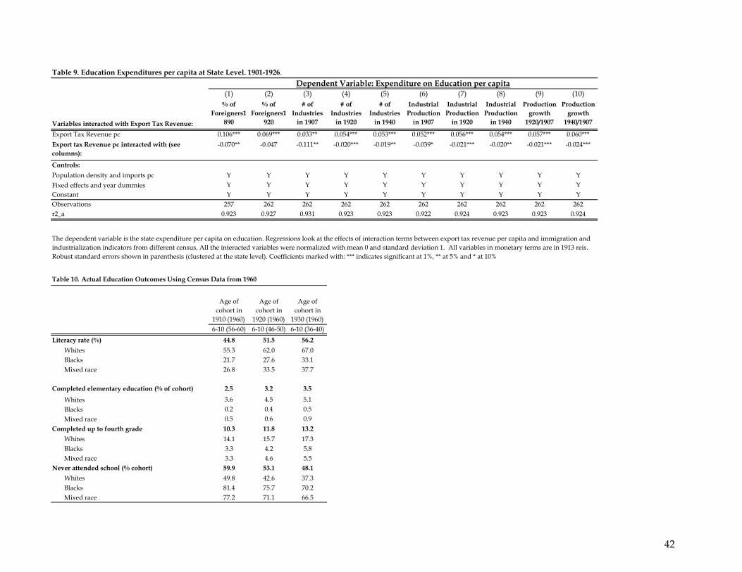
(1) (2) (3) (4) (5) (6) (7) (8) (9) (10)

Variables interacted with Export Tax Revenue:

% of Foreigners1

890

% of Foreigners1

920

# of Industries

in 1907

# of Industries

in 1920

# of Industries

in 1940

Industrial Production

in 1907

Industrial Production

in 1920

Industrial Production

in 1940

Production growth

1920/1907

Production growth

1940/1907

Export Tax Revenue pc 0.106*** 0.069*** 0.033** 0.054*** 0.053*** 0.052*** 0.056*** 0.054*** 0.057*** 0.060***

Export tax Revenue pc interacted with (see columns):

-0.070** -0.047 -0.111** -0.020*** -0.019** -0.039* -0.021*** -0.020** -0.021*** -0.024***

Controls:

Population density and imports pc Y Y Y Y Y Y Y Y Y Y

Fixed effects and year dummies Y Y Y Y Y Y Y Y Y YConstant Y Y Y Y Y Y Y Y Y YObservations 257 262 262 262 262 262 262 262 262 262r2_a 0.923 0.927 0.931 0.923 0.923 0.922 0.924 0.923 0.923 0.924

Table 10. Actual Education Outcomes Using Census Data from 1960

Age of cohort in

1910 (1960)

Age of cohort in

1920 (1960)

Age of cohort in

1930 (1960)6-10 (56-60) 6-10 (46-50) 6-10 (36-40)

Literacy rate (%) 44.8 51.5 56.2

Whites 55.3 62.0 67.0Blacks 21.7 27.6 33.1Mixed race 26.8 33.5 37.7

Completed elementary education (% of cohort) 2.5 3.2 3.5

Whites 3.6 4.5 5.1

Blacks 0.2 0.4 0.5

Mixed race 0.5 0.6 0.9

Completed up to fourth grade 10.3 11.8 13.2

Whites 14.1 15.7 17.3Blacks 3.3 4.2 5.8Mixed race 3.3 4.6 5.5

Never attended school (% cohort) 59.9 53.1 48.1

Whites 49.8 42.6 37.3Blacks 81.4 75.7 70.2Mixed race 77.2 71.1 66.5

Table 9. Education Expenditures per capita at State Level. 1901-1926.

Dependent Variable: Expenditure on Education per capita

The dependent variable is the state expenditure per capita on education. Regressions look at the effects of interaction terms between export tax revenue per capita and immigration and industrialization indicators from different census. All the interacted variables were normalized with mean 0 and standard deviation 1. All variables in monetary terms are in 1913 reis. Robust standard errors shown in parenthesis (clustered at the state level). Coefficients marked with: *** indicates significant at 1%, ** at 5% and * at 10%

42