Electronic-Vibrational Coupling

Colors of Co(III) solutions

Vibronic Coupling

★ Because they have g—g character, the d-d transitions of complexes of the transition metals are “forbidden” (LaPorte forbidden).

★ Complexes with noncentrosymmetric coordination geometries (e.g., tetrahedral) have more intense d-d spectra.

★ Spectra in centrosymmetric (e.g., octahedral) complexes “acquire intensity” via vibronic coupling.

The total molecular wavefunction can usually be approximated as a product of electronic, vibrational, and rotational parts:

H ΨIt is good first approximation to assume that electronic,

vibrational, and rotational motion can be separated: H ≈ H elec. + H vib. + H rot.

In this approximation, the wavefunction is a product: Ψ =ψ elec.ψ vib.ψ rot.

H Ψ =ψ vib.ψ rot. H elec.ψ elec.( ) ++ψ elec.ψ rot. H vib.ψ vib.( ) +ψ elec.ψ vib. H rot.ψ rot.( )

H Ψ = Eelec. + Evib. + Erot.( )ΨHowever, the "separability" is not exact.

More accurately, H ≈ H elec. + H vib. + H rot . + H elec-vib

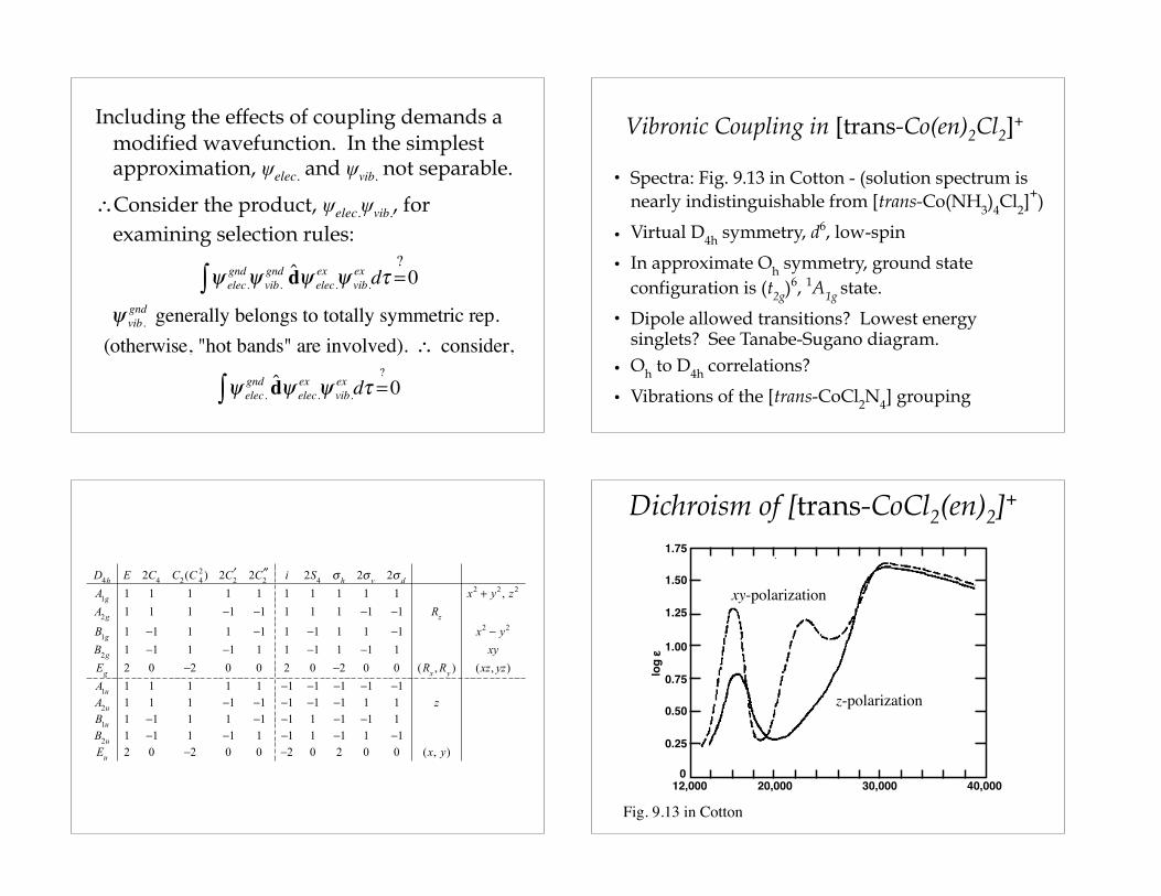
Including the effects of coupling demands a modified wavefunction. In the simplest approximation, ψelec. and ψvib. not separable.

∴Consider the product, ψelec.ψvib., for examining selection rules:

ψ elec.gndψ vib.

gnd d̂ψ elec.ex ψ vib.

ex∫ dτ =?

0

ψ vib.gnd generally belongs to totally symmetric rep.

(otherwise, "hot bands" are involved). ∴ consider,

ψ elec.gnd d̂ψ elec.

ex ψ vib.ex∫ dτ =

?0

Vibronic Coupling in [trans-Co(en)2Cl2]+

• Spectra: Fig. 9.13 in Cotton - (solution spectrum is nearly indistinguishable from [trans-Co(NH3)4Cl2]

+)

• Virtual D4h symmetry, d6, low-spin

• In approximate Oh symmetry, ground state configuration is (t2g)

6, 1A1g state.

• Dipole allowed transitions? Lowest energy singlets? See Tanabe-Sugano diagram.

• Oh to D4h correlations?

• Vibrations of the [trans-CoCl2N4] grouping

D4h E 2C4 C2(C 42 ) 2C2

′ 2C2′′ i 2S4 σ h 2σ v 2σ d

A1g 1 1 1 1 1 1 1 1 1 1 x2 + y2 , z2

A2g 1 1 1 −1 −1 1 1 1 −1 −1 Rz

B1g 1 −1 1 1 −1 1 −1 1 1 −1 x2 − y2

B2g 1 −1 1 −1 1 1 −1 1 −1 1 xyEg 2 0 −2 0 0 2 0 −2 0 0 (Rx , Ry ) (xz, yz)A1u 1 1 1 1 1 −1 −1 −1 −1 −1A2u 1 1 1 −1 −1 −1 −1 −1 1 1 zB1u 1 −1 1 1 −1 −1 1 −1 −1 1B2u 1 −1 1 −1 1 −1 1 −1 1 −1Eu 2 0 −2 0 0 −2 0 2 0 0 (x, y)

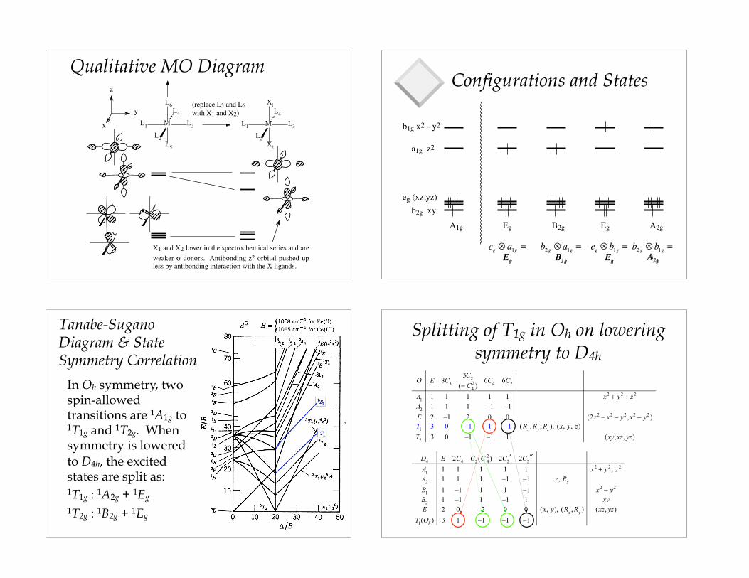
Dichroism of [trans-CoCl2(en)2]+

Fig. 9.13 in Cotton

12,000 20,000 30,000 40,0000

0.25

0.50

0.75

1.00

1.25

1.50

1.75

log ε

z-polarization

xy-polarization

Qualitative MO Diagram

y

z

x

(replace L5 and L6 with X1 and X2)

M L3L1

L2

L4

X1

X2

L6

M L3L1

L5

L2

L4

X1 and X2 lower in the spectrochemical series and are weaker σ donors. Antibonding z2 orbital pushed up less by antibonding interaction with the X ligands.

Configurations and States

a1g z2

b1g x2 - y2

b2g xyeg (xz,yz)

A1g Eg B2g Eg A2g

eg ⊗ a1g =Eg

b2g ⊗ a1g =B2g

eg ⊗ b1g =Eg

b2g ⊗ b1g =A2gEg B2g Eg A2g

Tanabe-Sugano Diagram & State Symmetry Correlation

In Oh symmetry, two spin-allowed transitions are 1A1g to 1T1g and 1T2g. When symmetry is lowered to D4h, the excited states are split as: 1T1g : 1A2g + 1Eg

1T2g : 1B2g + 1Eg

Splitting of T1g in Oh on lowering symmetry to D4h

O E 8C33C2

(= C42 )

6C4 6C2

A1 1 1 1 1 1 x2 + y2 + z2

A2 1 1 1 –1 –1E 2 –1 2 0 0 (2z2 – x2 − y2,x2 − y2 )T1 3 0 –1 1 –1 (Rx ,Ry ,Rz ); (x, y, z)T2 3 0 –1 –1 1 (xy,xz, yz)

D4 E 2C4 C2(C 42 ) 2C2

′ 2C2′′

A1 1 1 1 1 1 x2 + y2, z2

A2 1 1 1 –1 –1 z, RzB1 1 –1 1 1 –1 x2 − y2

B2 1 –1 1 –1 1 xyE 2 0 –2 0 0 (x, y), (Rx ,Ry ) (xz, yz)

T1(Oh ) 3 1 −1 −1 −1

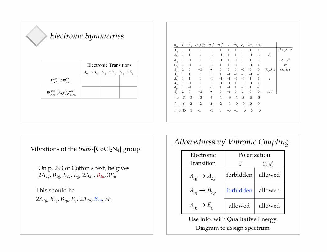
Electronic Symmetries

Electronic TransitionsA1g → A1g A1g → B2g A1g → Eg

ψ elec.gnd zψ elec.

ex

ψ elec.gnd (x,y)ψ elec.

ex

Γall 21 3 –3 –3 –1 –3 –1 5 5 3

Γt+r 6 2 –2 –2 –2 0 0 0 0 0

Γvib 15 1 –1 –1 1 –3 –1 5 5 3

D4h E 2C4 C2(C 42 ) 2C2

′ 2C2′′ i 2S4 σ h 2σ v 2σ d

A1g 1 1 1 1 1 1 1 1 1 1 x2 + y2 , z2

A2g 1 1 1 −1 −1 1 1 1 −1 −1 Rz

B1g 1 −1 1 1 −1 1 −1 1 1 −1 x2 − y2

B2g 1 −1 1 −1 1 1 −1 1 −1 1 xyEg 2 0 −2 0 0 2 0 −2 0 0 (Rx , Ry ) (xz, yz)A1u 1 1 1 1 1 −1 −1 −1 −1 −1A2u 1 1 1 −1 −1 −1 −1 −1 1 1 zB1u 1 −1 1 1 −1 −1 1 −1 −1 1B2u 1 −1 1 −1 1 −1 1 −1 1 −1Eu 2 0 −2 0 0 −2 0 2 0 0 (x, y)

Vibrations of the trans-[CoCl2N4] group

_ On p. 293 of Cotton’s text, he gives 2A1g, B1g, B2g, Eg, 2A2u, B1u, 3Eu

This should be 2A1g, B1g, B2g, Eg, 2A2u, B2u, 3Eu

Allowedness w/ Vibronic Coupling

Use info. with Qualitative Energy Diagram to assign spectrum

Electronic Transition

Polarization z (x,y)

forbidden allowed

forbidden allowed

allowed allowed

A1g → A2g

A1g → B2g

A1g → Eg

Graphical Summary• Because of the Oh → D4h

symmetry correlations, the specific configurations shown correspond to only the states shown - even in Oh .

• The dashed transitions are dipole and vibronically forbidden in z-polarization.

• The x,y-polarized transition at ~23,000 cm–1 is difficult to assign. The 1B2g state should be relatively favored by the weaker ligand field of the Cl ligands, but there is less e–-e– repulsion in the 1A2g state. 1A1g

xyx2-y2

xyz2

1T1g

1T2g

1Eg

1B2g1A2g

1Eg

xy

x2-y2z2

xy

x2-y2z2

Oh D4h

1A1g

Oh: E(1T2g ) − E(1T1g ) = 16B ≈ 17000 cm–1

Graphical Tools for getting relative Energies of States

Energies of each configuration are given by counting the orbital energies, adding up the repulsions (Jij) and subtracting the exchange “stabilizations” (Kij) between like spins.

A Graphical Scheme for getting relative Energies of States

Egr = 2εa + 2εb + Ja,a + Jb,b + 4Ja,b − 2Ka,b

Eex(3) = 2εa + εb + εc + Ja,a + 2Ja,b + 2Ja,c + Jb,c − Ka,b + Ka,c( ) − Kb,c

EexA = 2εa + εb + εc + Ja,a + 2Ja,b + 2Ja,c + Jb,c − Ka,b + Ka,c( )

EexB = 2εa + εb + εc + Ja,a + 2Ja,b + 2Ja,c + Jb,c − Ka,b + Ka,c( )

EexA+B + Eex

A−B = EexA + Eex

B ; but EexA+B = Eex

(3) and EexA−B = Eex

(1)

∴Eex(1) = Eex

A + EexB − Eex

(3)

Eex(1) = 2εa + εb + εc + Ja,a + 2Ja,b + 2Ja,c + Jb,c − Ka,b + Ka,c( ) + Kb,c

Eex(1) − Eex

(3) = +2Kb,c

A Graphical Scheme for getting relative Energies of States

Complex d-orbital J and K’s

The Coulomb (Jij) and exchange (Kij) integrals shown here can often be used to calculate state energy differences.

For 1st row transition metals, Racah parameters B and C have typical ranges shown. (State energy differences don’t involve A .)

J0,0 A+ 4B + 3CJ2,2 = J−2,−2 = J2,−2 A+ 4B + 2CJ2,1 = J−2,−1 = J2,−1 = J−2,1 A− 2B + CJ2,0 = J−2,0 A− 4B + CJ1,1 = J−1,−1 = J1,−1 A+ B + 2CJ1,0 = J−1,0 A+ 2B + CK1,−1 6B + 2CK2,−2 CK2,1 = K−2,−1 6B + CK2,−1 = K−2,1 CK2,0 = K−2,0 4B + CK1,0 = K−1,0 B + C

B ≈ 650 −1100 cm−1 C ≈ 2500 − 5500 cm−1

Slater-Condon and Racah Parameters

The "Slater-Condon parameters" are defined by

F k ≡ e2 r12

0

∞

∫ r22

0

∞

∫r<

k

r>k+1

Rnl (r1)2

Rnl (r2 )2

dr2

⎡

⎣⎢⎢

⎤

⎦⎥⎥

dr1 ; r<

k

r>k+1

=

r1k

r2k+1

if r2 > r1

r2k

r1k+1

if r1 > r2

⎧

⎨

⎪⎪

⎩

⎪⎪

and (in the d-shell): F0 ≡ F 0 , F2 =F 2

49 , F4 =

F 4

441The "Racah Parameters" are related to the Slater-Condon parameters by

A = F0 − 49F4

B = F2 − 5F4

C = 35F4

Example: B parameter for V3+

3F state: |3F ; 3 1⟩ = | 2+1+⟩ E(3F) = 2hd + J2,1 – K2,1 = 2hd + (A – 2B + C) – (6B + C) = 2hd + A – 8B

3P state: |3P ; 1 1 ⟩ = √3/5 |1

+ 0+ ⟩ – √2/5 |2+ –1+ ⟩

E(1+ 0+) = 2hd + J1,0 – K1,0 = 2hd + (A + 2B + C) – (B + C) = 2hd + A + B E(2+ –1+) = 2hd + J2,–1 – K2,–1 = 2hd + (A – 2B + C) – C = 2hd + A – 2B E(3P) = E(1+ 0+) + E(2+ –1+) – E(3F) = 2hd + A + 7B

E(3P) – E(3F) = 15B = 12,924 cm–1 B = 861.7 cm–1

Energies of d2 and d3 Terms

N Term Symbol Slater–Condon

Expression

Racah Expression

3F F0 – 8F2 – 9F4 A – 8B

3P F0 + 7F2 – 84F4 A + 7B

d2 1G F0 + 4F2 + F4 A + 4B + 2C

1D F0 – 3F2 + 36F4 A – 3B + 2C

1S F0 + 14F2 – 126F4 A + 14B + 7C

4F 3F0 – 15F2 – 72F4 3A – 15B

4P 3F0 – 147F4 3 A

2H 3F0 – 6F2 – 12F4 3A – 6B + 3C

d3 2P 3F0 – 6F2 – 12F4 3A – 6B + 3C

2G 3F0 – 11F2 + 13F4 3A – 11B + 3C

2F 3F0 + 9F2 – 87F4 3A + 9B + 3C

2D = 3, + = 1, –

3F0 + 5F2 + 3F4 ± (193F2

2 – 1650F2F4 + 8325F4

2)1/2

3A – 3B + 5C ± (193B2 + 8BC + 4C2)1/2

Tanabe-Sugano ∆E’s and the Scheme

Worked out details: singlet states example for the high-field limit for the d6 case.

1A1g : 6εt2g+ 3Jxy,xy +12Jxy,xz − 6Kxy,xz

1T1g : 5εt2g+ εeg

+ 2Jxy,xy + Jx2 − y2 ,xy

+12Jxy,xz − 6Kxy,xz + Kx2 − y2 ,xy

1T2g : 5εt2g+ εeg

+ 2Jxy,xy + Jxy,z2 + 8Jxy,xz + 4J

xz ,z2 − 4Kxy,xz − 2Kxz ,z2 + K

xy,z2

E(1T2g ) − E(1T1g ) =

Jxy,z2 − J

x2 − y2 ,xy( ) + 4 Jxz ,z2 − Jxy,xz( ) + 2 Kxy,xz − K

xz ,z2( ) + Kxy,z2 − K

x2 − y2 ,xy( )= −8B + 4(4B) + 2(3B − B) + (4B − 0) = 16B

Note: The exchange contributions are positive because these are the singlet states - see the diagram - back four slides!

Some Coulomb and Exchange Integrals

The Coulomb (Jij) and exchange (Kij) integrals shown here can often be used to calculate state energy differences.

Coulomb and Exchange Integrals Racah ParametersJxy,xy = Jxz ,xz = J yz , yz = J

z2 ,z2 = Jx2 − y2 ,x2 − y2 A+ 4B + 3C

Jxz , yz = Jxy, yz = Jxy,xz = Jx2 − y2 , yz

= Jx2 − y2 ,xz

A− 2B + C

Jxy,z2 = J

x2 − y2 ,z2 A− 4B + C

Jyz ,z2 = J

xz ,z2 A+ 2B + C

Jx2 − y2 ,xy

A+ 4B + C

Kxy, yz = Kxz , yz = Kxy,xz = Kx2 − y2 , yz

= Kx2 − y2 ,xz

3B + C

Kxy,z2 = K

x2 − y2 ,z2 4B + C

Kyz ,z2 = K

xz ,z2 B + C

Kx2 − y2 ,xy

C

∫ϕxz (1)ϕxy (2) 1 r12( )ϕ yz (1)ϕx2 − y2 (2)dτ1dτ2 −3B

B ≈ 650 −1100 cm−1 C ≈ 2500 − 5500 cm−1

For 1st row transition metals, Racah parameters B and C have typical ranges shown. (State energy differences don’t involve A .)

CrIII d-d spectra

[Cr(H2O)6]3+

[Cr(en)3]3+

300 350 400 450 500 550 600 650 700

174222457021834

28490

λ (nm)

Nonlinear Molecules in orbitally degenerate states are inherently unstable with respect to distortion.

We can write the ground state electronic energy, E0(Q), as a series expansion in each normal coordinate, Q:

Q - belongs to non-totally symmetric rep.

Jahn-Teller Theorem

E0 (Q) = E00 + E0

1(Q)Q + E02 (Q)Q2 + ...

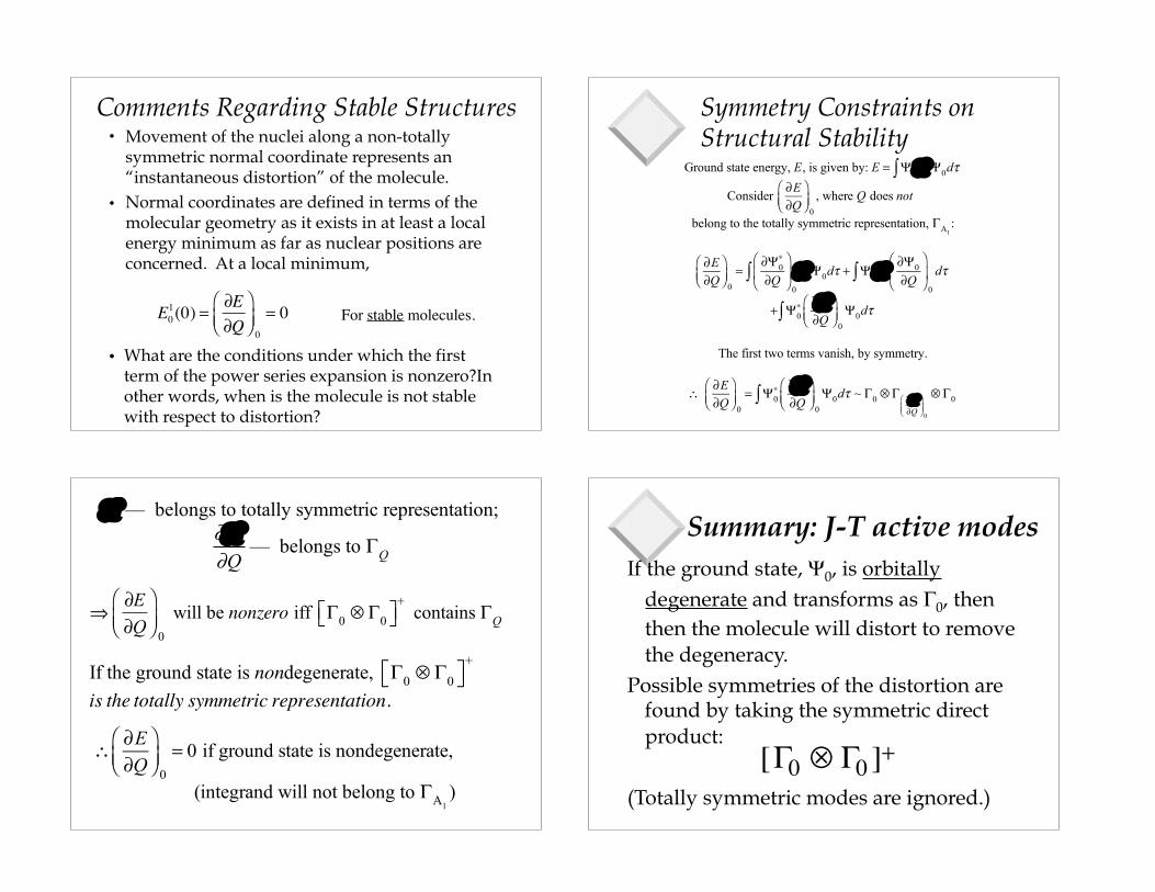
Comments Regarding Stable Structures

For stable molecules.

• Movement of the nuclei along a non-totally symmetric normal coordinate represents an “instantaneous distortion” of the molecule.

• Normal coordinates are defined in terms of the molecular geometry as it exists in at least a local energy minimum as far as nuclear positions are concerned. At a local minimum,

What are the conditions under which the first term of the power series expansion is nonzero?In other words, when is the molecule is not stable with respect to distortion?

•

E01(0) = ∂E

∂Q⎛⎝⎜

⎞⎠⎟ 0

= 0

Symmetry Constraints on Structural Stability

Ground state energy, E, is given by: E = Ψ0∗∫ H Ψ0dτ

Consider ∂E∂Q

⎛⎝⎜

⎞⎠⎟ 0

, where Q does not

belong to the totally symmetric representation, ΓA1:

∂E∂Q

⎛⎝⎜

⎞⎠⎟ 0

=∂Ψ0

∗

∂Q

⎛

⎝⎜

⎞

⎠⎟

0∫ H Ψ0dτ + Ψ0

∗∫ H∂Ψ0

∂Q⎛

⎝⎜

⎞

⎠⎟

0

dτ

+ Ψ0∗∫

∂H∂Q

⎛⎝⎜

⎞⎠⎟ 0

Ψ0dτ

The first two terms vanish, by symmetry.

∴ ∂E∂Q

⎛⎝⎜

⎞⎠⎟ 0

= Ψ0∗∫

∂H∂Q

⎛⎝⎜

⎞⎠⎟ 0

Ψ0dτ ~ Γ0 ⊗Γ ∂H∂Q

⎛⎝⎜

⎞⎠⎟ 0

⊗Γ0

H — belongs to totally symmetric representation;

∂H∂Q

— belongs to ΓQ

⇒

∂E∂Q

⎛⎝⎜

⎞⎠⎟ 0

will be nonzero iff Γ0 ⊗Γ0⎡⎣ ⎤⎦+

contains ΓQ

If the ground state is nondegenerate, Γ0 ⊗Γ0⎡⎣ ⎤⎦+

is the totally symmetric representation.

∴ ∂E∂Q

⎛⎝⎜

⎞⎠⎟ 0

= 0 if ground state is nondegenerate,

(integrand will not belong to ΓA1)

Summary: J-T active modesIf the ground state, Ψ0, is orbitally

degenerate and transforms as Γ0, then then the molecule will distort to remove the degeneracy.

Possible symmetries of the distortion are found by taking the symmetric direct product:

(Totally symmetric modes are ignored.)

[Γ0 ⊗ Γ0 ]+

Examples★ The best known J-T unstable molecules are Cu

II d

9

“octahedral” cases. What is the expected distortion coordinate?

★ “Tetrahedral” CuII complexes are common. Are they

really tetrahedral? ★ Are octahedral Ni

II complexes J-T unstable, (i) in their

ground states?, (ii) in excited states of the ground configuration?

★ Is cyclobutadiene J-T unstable, (i) in its ground state?, (ii) in excited states of the ground configuration?

★ What is the expected structure of the CrN36–

ion (in Ca3(CrN3))?

★ Would an octahedral VIII

complex be expected to exhibit a J-T distortion?

O E 8C33C2

(= C42 )

6C4 6C2

A1 1 1 1 1 1 x2 + y2 + z2

A2 1 1 1 –1 –1E 2 –1 2 0 0 (2z2 – x2 − y2 ,x2 − y2 )T1 3 0 –1 1 –1 (Rx , Ry , Rz ); (x, y, z)T2 3 0 –1 –1 1 (xy,xz, yz)

D4 E 2C4 C2(C 42 ) 2C2

′ 2C2′′

A1 1 1 1 1 1 x2 + y2, z2

A2 1 1 1 –1 –1 z, RzB1 1 –1 1 1 –1 x2 − y2

B2 1 –1 1 –1 1 xyE 2 0 –2 0 0 (x, y), (Rx ,Ry ) (xz, yz)

[E⊗ E]– 1 1 1 −1 −1 = A2[E⊗ E]+ 3 −1 3 1 1 = A1⊕ B1⊕ B2

Tetrahedral Group: Td

Td E 8C3 3C2 6S4 6σ d

A1 1 1 1 1 1 x2 + y2 + z2

A2 1 1 1 –1 –1E 2 –1 2 0 0 (2z2 – x2 − y2 , x2 − y2 )T1 3 0 –1 1 –1 (Rx , Ry , Rz )T2 3 0 –1 –1 1 (x, y, z) (xy,xz, yz)

D3h

D3h E 2C3 3C2 σ h 2S3 3σ v

A1′ 1 1 1 1 1 1 x2 + y2 , z2

A2′ 1 1 −1 1 1 −1 Rz

′E 2 −1 0 2 −1 0 (x, y) (x2 − y2 ,xy)A1′′ 1 1 1 −1 −1 −1

A2′′ 1 1 −1 −1 −1 1 z′′E 2 −1 0 −2 1 0 (Rx , Ry ) (xz, yz)

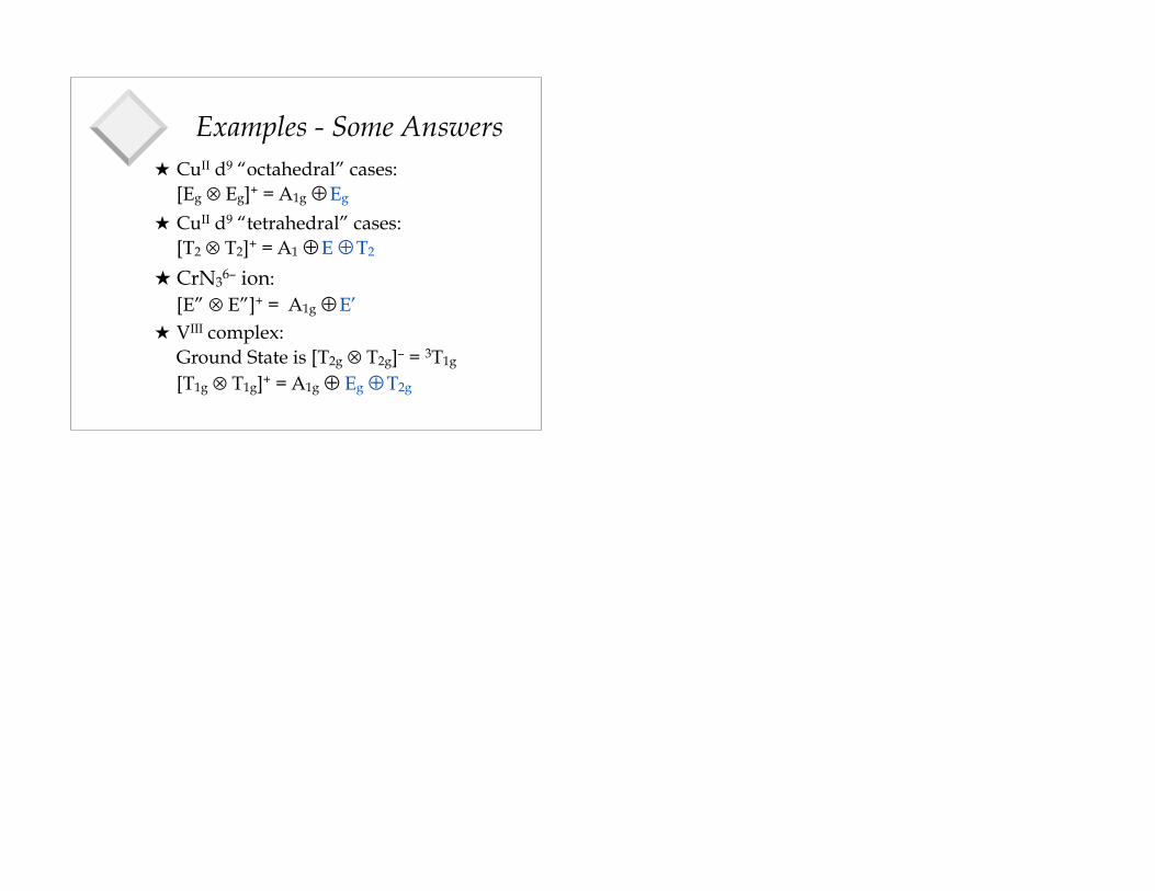
Examples - Some Answers★ CuII d9 “octahedral” cases:

[Eg ⊗ Eg]+ = A1g ⊕ Eg

★ CuII d9 “tetrahedral” cases: [T2 ⊗ T2]+ = A1 ⊕ E ⊕ T2

★ CrN36– ion: [E” ⊗ E”]+ = A1g ⊕ E’

★ VIII complex: Ground State is [T2g ⊗ T2g]– = 3T1g [T1g ⊗ T1g]+ = A1g ⊕ Eg ⊕ T2g