combinatorial auctions with restricted … auctions with restricted complements shaddin dughmi joint...
TRANSCRIPT

Combinatorial Auctions with Restricted Complements
Shaddin Dughmi
Joint work with:Ittai Abraham
Moshe BabaioffTim Roughgarden
April 12, 2012

Outline
1 Introduction
2 Technical Background
3 A Polylog Approximation Mechanism
4 Future Work

Outline
1 Introduction
2 Technical Background
3 A Polylog Approximation Mechanism
4 Future Work

Combinatorial Auctions
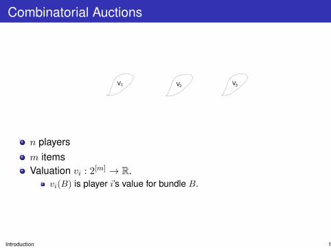
n players
m itemsValuation vi : 2[m] → R.
vi(B) is player i’s value for bundle B.
GoalPartition items into bundles B1, B2, . . . , Bn to maximize welfare:v1(B1) + v2(B2) + . . . + vn(Bn)
Introduction 1

Combinatorial Auctions
n playersm items
Valuation vi : 2[m] → R.vi(B) is player i’s value for bundle B.
GoalPartition items into bundles B1, B2, . . . , Bn to maximize welfare:v1(B1) + v2(B2) + . . . + vn(Bn)
Introduction 1
Combinatorial Auctions
V1 V2 V3
n playersm itemsValuation vi : 2[m] → R.
vi(B) is player i’s value for bundle B.
GoalPartition items into bundles B1, B2, . . . , Bn to maximize welfare:v1(B1) + v2(B2) + . . . + vn(Bn)
Introduction 1

Combinatorial Auctions
V1 V2 V3
n playersm itemsValuation vi : 2[m] → R.
vi(B) is player i’s value for bundle B.
GoalPartition items into bundles B1, B2, . . . , Bn to maximize welfare:v1(B1) + v2(B2) + . . . + vn(Bn)
Introduction 1
Combinatorial Auctions
V1 V2 V3
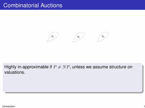
Highly in-approximable if P 6= NP , unless we assume structure onvaluations.
We will consider a classes of valuations allowing constant factorapproximation algorithms.
Introduction 1

Combinatorial Auctions
V1 V2 V3
Highly in-approximable if P 6= NP , unless we assume structure onvaluations.
We will consider a classes of valuations allowing constant factorapproximation algorithms.
Introduction 1

Example: Spectrum Auctions
Each telecom has a private value in $$ for each bundle of licensesDependencies: Some of the licenses are substitutes/complements
Introduction 2

Importance of Combinatorial AuctionsParadigmatic problem in algorithmic mechanism design.Many applications.Theoretically clean and expressive.
GoalAssuming valuations come from a class that naturally models someapplication, we want a mechanism that is:
1 (Dominant strategy) incentive compatible (truthful in expectation)2 Polynomial time3 Guarantees a “good” approximation to the social welfare
Constant factorClose to best of a polynomial time approximation algorithm
For which valuation classes is this possible?
Introduction 3

Previous Work
Positive Results:O(logm log logm) for subadditive, demand oracle. [Dobzinski ’07]O(logm/ log logm) for submodular, communication.[Dobzinski, Fu, Kleinberg ’10]1− 1/e for coverage valuations, computational.[Dughmi, Roughgarden, Yan ’11]
Negative Results:Ω(mα) for submodular, value oracle. [Dughmi, Vondrak ’11]Ω(nα) for submodular, computational. [Dobzinski, Vondrak ’12]
Introduction 4

This Sucks
1 Only “good” upperbounds are for complement free valuationsIn practice complements are present, and are the main obstacle.
2 Lower bounds are fragileRely on hardness of single-player utility maximization.Fall apart when we assume access to a demand oracle.
Introduction 5

This Sucks
1 Only “good” upperbounds are for complement free valuationsIn practice complements are present, and are the main obstacle.
2 Lower bounds are fragileRely on hardness of single-player utility maximization.Fall apart when we assume access to a demand oracle.
Introduction 5
Modeling Complements
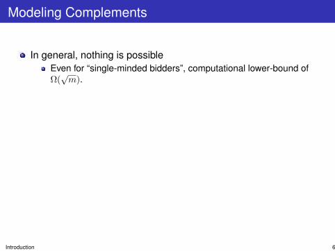
In general, nothing is possibleEven for “single-minded bidders”, computational lower-bound ofΩ(√m).
Ideally, want a model that is:1 Parametrized by the “size” of complements2 Admits approximation algorithms with guarantees that degrade
gracefully with size of complements.3 Succinct4 Admits a polynomial-time demand oracle
This PaperWe consider a such a natural model for combinatorial auctions withcomplements.
Introduction 6

Modeling Complements
In general, nothing is possibleEven for “single-minded bidders”, computational lower-bound ofΩ(√m).
Ideally, want a model that is:1 Parametrized by the “size” of complements2 Admits approximation algorithms with guarantees that degrade
gracefully with size of complements.
3 Succinct4 Admits a polynomial-time demand oracle
This PaperWe consider a such a natural model for combinatorial auctions withcomplements.
Introduction 6

Modeling Complements
In general, nothing is possibleEven for “single-minded bidders”, computational lower-bound ofΩ(√m).
Ideally, want a model that is:1 Parametrized by the “size” of complements2 Admits approximation algorithms with guarantees that degrade
gracefully with size of complements.3 Succinct
4 Admits a polynomial-time demand oracle
This PaperWe consider a such a natural model for combinatorial auctions withcomplements.
Introduction 6

Modeling Complements
In general, nothing is possibleEven for “single-minded bidders”, computational lower-bound ofΩ(√m).
Ideally, want a model that is:1 Parametrized by the “size” of complements2 Admits approximation algorithms with guarantees that degrade
gracefully with size of complements.3 Succinct4 Admits a polynomial-time demand oracle
This PaperWe consider a such a natural model for combinatorial auctions withcomplements.
Introduction 6

Modeling Complements
In general, nothing is possibleEven for “single-minded bidders”, computational lower-bound ofΩ(√m).
Ideally, want a model that is:1 Parametrized by the “size” of complements2 Admits approximation algorithms with guarantees that degrade
gracefully with size of complements.3 Succinct4 Admits a polynomial-time demand oracle
This PaperWe consider a such a natural model for combinatorial auctions withcomplements.
Introduction 6

(Hyper) graph valuations
Valuation of a player i described by a graph on the items.Weights vi(j) ≥ 0 on nodes jWeights vi(j, k) ≥ 0 on edges (j, k)vi(S) =
∑j∈S vi(j) +
∑j,k∈S vi(j, k)
10 5
7 2
2
3 1
0
5
Generalizing to hypergraphs, we model k-complements as ak-hypergraph valuation.Similar to models proposed earlier in the literature [Conitzer,Sandholm, and Santi ’05, Chevaleyre et al ’08].
Introduction 7

(Hyper) graph valuations
Valuation of a player i described by a graph on the items.Weights vi(j) ≥ 0 on nodes jWeights vi(j, k) ≥ 0 on edges (j, k)vi(S) =
∑j∈S vi(j) +
∑j,k∈S vi(j, k)
10 5
7 2
2
3 1
0
5
Generalizing to hypergraphs, we model k-complements as ak-hypergraph valuation.
Similar to models proposed earlier in the literature [Conitzer,Sandholm, and Santi ’05, Chevaleyre et al ’08].
Introduction 7

(Hyper) graph valuations
Valuation of a player i described by a graph on the items.Weights vi(j) ≥ 0 on nodes jWeights vi(j, k) ≥ 0 on edges (j, k)vi(S) =
∑j∈S vi(j) +
∑j,k∈S vi(j, k)
10 5
7 2
2
3 1
0
5
Generalizing to hypergraphs, we model k-complements as ak-hypergraph valuation.Similar to models proposed earlier in the literature [Conitzer,Sandholm, and Santi ’05, Chevaleyre et al ’08].
Introduction 7

Example: Spectrum Auctions
9
8
5
Introduction 8

Results
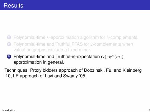
1 Polynomial-time k-approximation algorithm for k-complements.2 Polynomial-time and Truthful PTAS for 2-complements when
valuation graphs exclude a fixed minor.3 Polynomial-time and Truthful-in-expectation O(logk(m))
approximation in general.
Techniques: Proxy bidders approach of Dobzinski, Fu, and Kleinberg’10, LP approach of Lavi and Swamy ’05.
Introduction 9

Results
1 Polynomial-time k-approximation algorithm for k-complements.2 Polynomial-time and Truthful PTAS for 2-complements when
valuation graphs exclude a fixed minor.3 Polynomial-time and Truthful-in-expectation O(logk(m))
approximation in general.
Techniques: Proxy bidders approach of Dobzinski, Fu, and Kleinberg’10, LP approach of Lavi and Swamy ’05.
Introduction 9

Outline
1 Introduction
2 Technical Background
3 A Polylog Approximation Mechanism
4 Future Work

Mechanisms and Truthfulness
Mechanism1 Bidding: Solicit valuations v1, . . . , vn : 2[m] → R2 Allocation: Compute “good” allocation B1, . . . , Bn3 Payment: Charge payments p0, . . . , pn
Truthfulness in ExpectationA mechanism is truthful in expectation if a player maximizes hisexpected utility by reporting his true valuation, regardless of reports ofothers.
utility(i) = vi(Bi)− pi
Technical Background 10

VCG Mechanism
Vickrey Clarke Groves (VCG) Mechanism for CA1 Solicit purported valuations v1, . . . , vn : 2[m] → R2 Find allocation (B∗1 , . . . , B
∗n) maximizing (purported) welfare:∑
i vi(B∗i )
3 Charge each player his externalityThe increase in (purported) welfare of other players if he drops out
Technical Background 11

VCG Mechanism
Vickrey Clarke Groves (VCG) Mechanism for CA1 Solicit purported valuations v1, . . . , vn : 2[m] → R2 Find allocation (B∗1 , . . . , B
∗n) maximizing (purported) welfare:∑
i vi(B∗i )
3 Charge each player his externalityThe increase in (purported) welfare of other players if he drops out
Theorem (Vickrey, Clarke, Groves)VCG is truthful
Technical Background 11

VCG Mechanism
Vickrey Clarke Groves (VCG) Mechanism for CA1 Solicit purported valuations v1, . . . , vn : 2[m] → R2 Find allocation (B∗1 , . . . , B
∗n) maximizing (purported) welfare:∑
i vi(B∗i )
3 Charge each player his externalityThe increase in (purported) welfare of other players if he drops out
ProblemWhen the allocation problem is NP-hard, VCG cannot be implementedin polynomial time.
Some “special” approximation algorithms, when plugged into VCG, pre-serve truthfulness and recover polytime.
Technical Background 11

Maximal in Distributional Range Algorithms
Maximal in Distributional Range
1 Fix subset R of distributions over allocations up-front, called thedistributional range.
Independent of player valuations2 Given player values, find the distribution in R maximizing
expected social welfare.3 Sample this distribution
Technical Background 12

Maximal in Distributional Range Algorithms
Maximal in Distributional Range1 Fix subset R of distributions over allocations up-front, called the
distributional range.Independent of player valuations
2 Given player values, find the distribution in R maximizingexpected social welfare.
3 Sample this distribution
Technical Background 12

Maximal in Distributional Range Algorithms
Output
V1 V2 V3
Maximal in Distributional Range1 Fix subset R of distributions over allocations up-front, called the
distributional range.Independent of player valuations
2 Given player values, find the distribution in R maximizingexpected social welfare.
3 Sample this distribution
Technical Background 12

Maximal in Distributional Range Algorithms
Maximal in Distributional Range1 Fix subset R of distributions over allocations up-front, called the
distributional range.Independent of player valuations
2 Given player values, find the distribution in R maximizingexpected social welfare.
3 Sample this distribution
Technical Background 12

Maximal in Distributional Range and Truthfulness
Plugging an MIDR algorithm into VCG yields a truthful-in-expectationmechanism
Simply VCG applied to the “smaller” problem of finding the bestlottery in R, which we solve optimally.
UpshotReduced designing a truthful mechanism to designing anapproximation algorithm of this MIDR variety.
Technical Background 13
Designing MIDR Algorithms
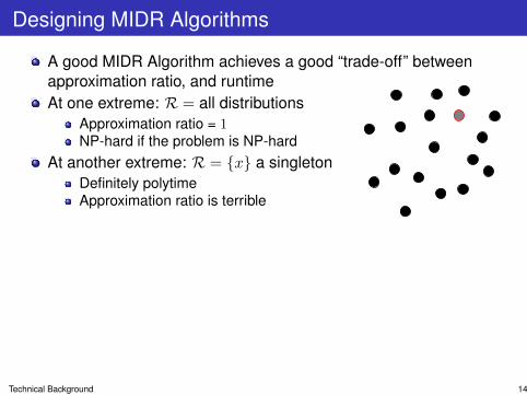
A good MIDR Algorithm achieves a good “trade-off” betweenapproximation ratio, and runtime
At one extreme: R = all distributionsApproximation ratio = 1NP-hard if the problem is NP-hard
At another extreme: R = x a singletonDefinitely polytimeApproximation ratio is terrible
Is there a “sweet spot”?Large enough for good approximationSmall/well-structured enough for polytime optimization
Technical Background 14

Designing MIDR Algorithms
A good MIDR Algorithm achieves a good “trade-off” betweenapproximation ratio, and runtimeAt one extreme: R = all distributions
Approximation ratio = 1NP-hard if the problem is NP-hard
At another extreme: R = x a singletonDefinitely polytimeApproximation ratio is terrible
Is there a “sweet spot”?Large enough for good approximationSmall/well-structured enough for polytime optimization
Technical Background 14

Example of MIDR
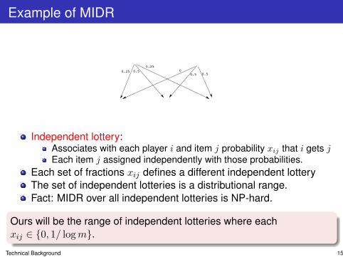
Independent lottery:Associates with each player i and item j probability xij that i gets jEach item j assigned independently with those probabilities.
Each set of fractions xij defines a different independent lotteryThe set of independent lotteries is a distributional range.Fact: MIDR over all independent lotteries is NP-hard.
Ours will be the range of independent lotteries where eachxij ∈ 0, 1/ logm.
Technical Background 15

Example of MIDR
0.50.25
0.250
0.5 0.5
Independent lottery:Associates with each player i and item j probability xij that i gets jEach item j assigned independently with those probabilities.
Each set of fractions xij defines a different independent lotteryThe set of independent lotteries is a distributional range.Fact: MIDR over all independent lotteries is NP-hard.
Ours will be the range of independent lotteries where eachxij ∈ 0, 1/ logm.
Technical Background 15

Example of MIDR
0.50.25
0.25
Independent lottery:Associates with each player i and item j probability xij that i gets jEach item j assigned independently with those probabilities.
Each set of fractions xij defines a different independent lotteryThe set of independent lotteries is a distributional range.Fact: MIDR over all independent lotteries is NP-hard.
Ours will be the range of independent lotteries where eachxij ∈ 0, 1/ logm.
Technical Background 15

Example of MIDR
00.5 0.5
Independent lottery:Associates with each player i and item j probability xij that i gets jEach item j assigned independently with those probabilities.
Each set of fractions xij defines a different independent lotteryThe set of independent lotteries is a distributional range.Fact: MIDR over all independent lotteries is NP-hard.
Ours will be the range of independent lotteries where eachxij ∈ 0, 1/ logm.
Technical Background 15

Example of MIDR
0.50.25
0.250
0.5 0.5
Independent lottery:Associates with each player i and item j probability xij that i gets jEach item j assigned independently with those probabilities.
Each set of fractions xij defines a different independent lotteryThe set of independent lotteries is a distributional range.
Fact: MIDR over all independent lotteries is NP-hard.
Ours will be the range of independent lotteries where eachxij ∈ 0, 1/ logm.
Technical Background 15

Example of MIDR
0.50.25
0.250
0.5 0.5
Independent lottery:Associates with each player i and item j probability xij that i gets jEach item j assigned independently with those probabilities.
Each set of fractions xij defines a different independent lotteryThe set of independent lotteries is a distributional range.Fact: MIDR over all independent lotteries is NP-hard.
Ours will be the range of independent lotteries where eachxij ∈ 0, 1/ logm.
Technical Background 15

Outline
1 Introduction
2 Technical Background
3 A Polylog Approximation Mechanism
4 Future Work

The Distributional Range
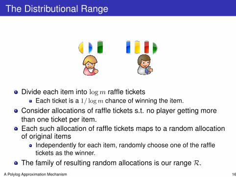
Divide each item into logm raffle ticketsEach ticket is a 1/ logm chance of winning the item.
Consider allocations of raffle tickets s.t. no player getting morethan one ticket per item.Each such allocation of raffle tickets maps to a random allocationof original items
Independently for each item, randomly choose one of the raffletickets as the winner.
The family of resulting random allocations is our range R.
A Polylog Approximation Mechanism 16

The Distributional Range
Divide each item into logm raffle ticketsEach ticket is a 1/ logm chance of winning the item.
Consider allocations of raffle tickets s.t. no player getting morethan one ticket per item.
Each such allocation of raffle tickets maps to a random allocationof original items
Independently for each item, randomly choose one of the raffletickets as the winner.
The family of resulting random allocations is our range R.
A Polylog Approximation Mechanism 16

The Distributional Range
Divide each item into logm raffle ticketsEach ticket is a 1/ logm chance of winning the item.
Consider allocations of raffle tickets s.t. no player getting morethan one ticket per item.Each such allocation of raffle tickets maps to a random allocationof original items
Independently for each item, randomly choose one of the raffletickets as the winner.
The family of resulting random allocations is our range R.
A Polylog Approximation Mechanism 16
The Distributional Range
Divide each item into logm raffle ticketsEach ticket is a 1/ logm chance of winning the item.
Consider allocations of raffle tickets s.t. no player getting morethan one ticket per item.Each such allocation of raffle tickets maps to a random allocationof original items
Independently for each item, randomly choose one of the raffletickets as the winner.
The family of resulting random allocations is our range R.A Polylog Approximation Mechanism 16

The Approximation Guarantee
LemmaFor every allocation (S1, . . . , Sn) of items, there is a lottery in the rangewith 1/ log2m fraction of the welfare.
Since we plan to optimize over the range, we will get a log2mapproximation.
A Polylog Approximation Mechanism 17

The Approximation Guarantee
LemmaFor every allocation (S1, . . . , Sn) of items, there is a lottery in the rangewith 1/ log2m fraction of the welfare.
Since we plan to optimize over the range, we will get a log2mapproximation.
A Polylog Approximation Mechanism 17

The Approximation Guarantee
Proof.Replace each item in each Si with a raffle ticket for that item.
Corresponds to a lottery in the range, by running raffles.
Consider an edge (j, k) with both endpoints in Si.He gets each of j,k with probability 1/ logm in the raffle.
Gets both with probability 1/ log2 m.
Since his utility is additive over edges, done.
2
31
A Polylog Approximation Mechanism 18

The Approximation Guarantee
Proof.Replace each item in each Si with a raffle ticket for that item.
Corresponds to a lottery in the range, by running raffles.
Consider an edge (j, k) with both endpoints in Si.
He gets each of j,k with probability 1/ logm in the raffle.Gets both with probability 1/ log2 m.
Since his utility is additive over edges, done.
2
31
A Polylog Approximation Mechanism 18

The Approximation Guarantee
Proof.Replace each item in each Si with a raffle ticket for that item.
Corresponds to a lottery in the range, by running raffles.
Consider an edge (j, k) with both endpoints in Si.He gets each of j,k with probability 1/ logm in the raffle.
Gets both with probability 1/ log2 m.
Since his utility is additive over edges, done.
2
31
A Polylog Approximation Mechanism 18

The Approximation Guarantee
Proof.Replace each item in each Si with a raffle ticket for that item.
Corresponds to a lottery in the range, by running raffles.
Consider an edge (j, k) with both endpoints in Si.He gets each of j,k with probability 1/ logm in the raffle.
Gets both with probability 1/ log2 m.
Since his utility is additive over edges, done.
2
31
A Polylog Approximation Mechanism 18

Optimizing over the Distributional Range
ObservationValue of player i for raffle tickets for Si is simply:
v′i(Si) = vi(Si)/ log2m
Therefore: Graph valuation with weights scaled down by log2m.Optimization problem for our range is combinatorial auctions withgraph valuations and logm supply of each item.
Fact (Folklore)A large linear programming relaxation, called the configuration LP, issolvable in polytime when valuations admit a demand oracle.
Fact (Informal)The configuration LP “essentially” has integrality gap 1 when we havelogm supply.
A Polylog Approximation Mechanism 19

Optimizing over the Distributional Range
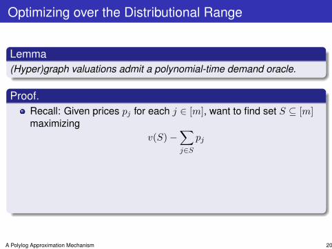
Lemma(Hyper)graph valuations admit a polynomial-time demand oracle.
Proof.Recall: Given prices pj for each j ∈ [m], want to find set S ⊆ [m]maximizing
v(S)−∑j∈S
pj
Rewriting, want to maximize∑
j∈S v(j) +∑
j,k∈S v(j, k)−∑
j∈S pj .Clearly supermodular, so can be maximized in polynomial time.
A Polylog Approximation Mechanism 20
Optimizing over the Distributional Range
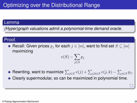
Lemma(Hyper)graph valuations admit a polynomial-time demand oracle.
Proof.Recall: Given prices pj for each j ∈ [m], want to find set S ⊆ [m]maximizing
v(S)−∑j∈S
pj
Rewriting, want to maximize∑
j∈S v(j) +∑
j,k∈S v(j, k)−∑
j∈S pj .Clearly supermodular, so can be maximized in polynomial time.
A Polylog Approximation Mechanism 20

Optimizing over the Distributional Range
Lemma(Hyper)graph valuations admit a polynomial-time demand oracle.
Proof.Recall: Given prices pj for each j ∈ [m], want to find set S ⊆ [m]maximizing
v(S)−∑j∈S
pj
Rewriting, want to maximize∑
j∈S v(j) +∑
j,k∈S v(j, k)−∑
j∈S pj .
Clearly supermodular, so can be maximized in polynomial time.
A Polylog Approximation Mechanism 20
Optimizing over the Distributional Range
Lemma(Hyper)graph valuations admit a polynomial-time demand oracle.
Proof.Recall: Given prices pj for each j ∈ [m], want to find set S ⊆ [m]maximizing
v(S)−∑j∈S
pj
Rewriting, want to maximize∑
j∈S v(j) +∑
j,k∈S v(j, k)−∑
j∈S pj .Clearly supermodular, so can be maximized in polynomial time.
A Polylog Approximation Mechanism 20

Outline
1 Introduction
2 Technical Background
3 A Polylog Approximation Mechanism
4 Future Work

Open Questions
1 Main open question: Is there a constant factor polytime truthfulmechanism for CA with restricted complements?
Existing results rule out deterministic VCG based.Existing techniques, such as Lavi/Swamy, proxy valuations, andConvex Rounding, don’t seem to work.
2 What about other classes of valuations, such as submodular, ifequipped with a demand oracle?
3 More generally: assuming individual agents can maximize theirown utility, does truthfulness + polytime follow?
4 Other ways of modeling complements?
Future Work 21

Thank You for Listening