Combinatorial interpretations of Lucas analogues ofbinomial coefficients and Catalan numbers

Curtis BennettDepartment of Mathematics, California State University,

Long Beach, CA 90840, USA, Curtis.Bennett@csulb.edu

Juan Carrillo20707 Berendo Avenue

Torrance, CA 90502, USA, juanscarrillo23@gmail.com

John MachacekDepartment of Mathematics and Statistics, York University,

Toronto, ON M3J 1P3, Canada, jmachacek.math@gmail.com

Bruce E. SaganDepartment of Mathematics, Michigan State University,

East Lansing, MI 48824, USA, sagan@math.msu.edu

September 24, 2018

Key Words: binomial coefficient, Catalan number, combinatorial interpretation, Coxeter group,generating function, integer partition, lattice path, Lucas sequence, tiling

AMS subject classification (2010): 05A10 (Primary) 05A15, 05A19, 11B39 (Secondary)

Abstract

The Lucas sequence is a sequence of polynomials in s, t defined recursively by {0} =0, {1} = 1, and {n} = s{n− 1}+ t{n− 2} for n ≥ 2. On specialization of s and t onecan recover the Fibonacci numbers, the nonnegative integers, and the q-integers [n]q.Given a quantity which is expressed in terms of products and quotients of nonnegativeintegers, one obtains a Lucas analogue by replacing each factor of n in the expressionwith {n}. It is then natural to ask if the resulting rational function is actually apolynomial in s, t with nonnegative integer coefficients and, if so, what it counts. Thefirst simple combinatorial interpretation for this polynomial analogue of the binomialcoefficients was given by Sagan and Savage, although their model resisted being used toprove identities for these Lucasnomials or extending their ideas to other combinatorialsequences. The purpose of this paper is to give a new, even more natural model forthese Lucasnomials using lattice paths which can be used to prove various equalitiesas well as extending to Catalan numbers and their relatives, such as those for finiteCoxeter groups.

1

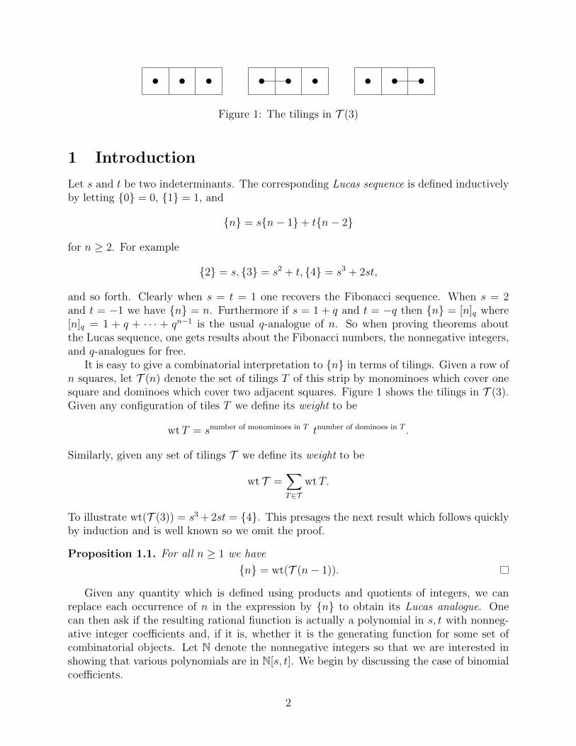
Figure 1: The tilings in T (3)

1 Introduction

Let s and t be two indeterminants. The corresponding Lucas sequence is defined inductivelyby letting {0} = 0, {1} = 1, and

{n} = s{n− 1}+ t{n− 2}

for n ≥ 2. For example

{2} = s, {3} = s2 + t, {4} = s3 + 2st,

and so forth. Clearly when s = t = 1 one recovers the Fibonacci sequence. When s = 2and t = −1 we have {n} = n. Furthermore if s = 1 + q and t = −q then {n} = [n]q where[n]q = 1 + q + · · · + qn−1 is the usual q-analogue of n. So when proving theorems aboutthe Lucas sequence, one gets results about the Fibonacci numbers, the nonnegative integers,and q-analogues for free.

It is easy to give a combinatorial interpretation to {n} in terms of tilings. Given a row ofn squares, let T (n) denote the set of tilings T of this strip by monominoes which cover onesquare and dominoes which cover two adjacent squares. Figure 1 shows the tilings in T (3).Given any configuration of tiles T we define its weight to be

wtT = snumber of monominoes in T tnumber of dominoes in T .

Similarly, given any set of tilings T we define its weight to be

wt T =∑T∈T

wtT.

To illustrate wt(T (3)) = s3 + 2st = {4}. This presages the next result which follows quicklyby induction and is well known so we omit the proof.

Proposition 1.1. For all n ≥ 1 we have

{n} = wt(T (n− 1)).

Given any quantity which is defined using products and quotients of integers, we canreplace each occurrence of n in the expression by {n} to obtain its Lucas analogue. Onecan then ask if the resulting rational fiunction is actually a polynomial in s, t with nonneg-ative integer coefficients and, if it is, whether it is the generating function for some set ofcombinatorial objects. Let N denote the nonnegative integers so that we are interested inshowing that various polynomials are in N[s, t]. We begin by discussing the case of binomialcoefficients.

2

1 2 3 4 5 6

1

2

3

4

5

6

1 2 3 4 5 6

1

2

3

4

5

6

Figure 2: δ6 embedded in R2 on the left and a tiling on the right.

For n ≥ 0, the Lucas analogue of a factorial is the Lucastorial

{n}! = {1}{2} . . . {n}.

Now given 0 ≤ k ≤ n we define the corresponding Lucasnomial to be{n

k

}=

{n}!{k}!{n− k}!

. (1)

It is not hard to see that this function satisfies an analogue of the binomial recursion (Propo-sition 3.1 below) and so inductively prove that it is in N[s, t].

The first simple combinatorial interpretation of the Lucasnomials was given by Sagan andSavage [SS10] using tilings of Young diagrams inside a rectangle. Earlier but more compli-cated models were given by Gessel and Viennot [GV85] and by Benjamin and Plott [BP09].Despite its simplicity, there were three difficulties with the Sagan-Savage approach. Themodel was not flexible enough to permit combinatorial demonstrations of straight-forwardidentities involving the Lucasnomials. Their ideas did not seem to extend to any other re-lated combinatorial sequences such as the Catalan numbers. And their model containedcertain dominoes in the tilings which appeared in an unintuitive manner. The goal of thispaper is to present a new construction which addresses these problems.

We should also mention related work on a q-version of these ideas. As noted above,letting s = t = 1 reduces {n} to Fn, the nth Fibonacci numbers. One can then makea q-Fibonacci analogue of a quotient of products by replacing each factor of n by [Fn]q.Working in this framework, some results parallel to ours were found indpendently during theworking sessions of the Algebraic Combinatorics Seminar at the Fields Institute with theactive participation of Farid Aliniaeifard, Nantel Bergeron, Cesar Ceballos, Tom Denton,and Shu Xiao Li [ABC+15].

3

We will need to consider lattice paths inside tilings of Young diagrams. Let λ =(λ1, λ2, . . . , λl) be an integer partition, that is, a weakly decreasing sequence of positiveintegers. The λi are called parts and the length of λ is the number of parts and denotedl(λ). The Young diagram of λ is an array of left-justified rows of boxes which we will writein French notation so that λi is the number of boxes in the ith row from the bottom ofthe diagram. We will also use the notation λ for the diagram of λ. Furthermore, we willembed this diagram in the first quadrant of a Cartesian coordinate system with the boxesbeing unit squares and the southwest-most corner of λ being the origin. Finally, it will beconvenient in what follows to consider the unit line segments from (λ1, 0) to (λ1 + 1, 0) andfrom (0, l(λ)) to (0, l(λ) + 1) to be part of λ’s diagram. On the left in Figure 2 the diagramof λ = δ6 is outlined with thick lines where

δn = (n− 1, n− 2, . . . , 1).

A tiling of λ is a tiling T of the rows of the diagram with monominoes and dominoes.We let T (λ) denote the set of all such tilings. An element of T (δ6) is shown on the rightin Figure 2. We write wtλ for the more cumbersome wt(T (λ)). The fact that wt δn = {n}!follows directly from the definitions. So to prove that {n}!/p(s, t) is a polynomial for somepolynomial p(s, t), it suffices to partition T (δn) into subsets, which we will call blocks, suchthat wt β is evenly divisible by p(s, t) for all blocks β. We will use lattice paths inside δn tocreate the partitions where the choice of path will vary depending on which Lucas analoguewe are considering.

The rest of this paper is organized as follows. In the next section, we give our newcombinatorial interpretation for the Lucasnomials. In Section 3 we prove two identitiesusing this model. The demonstration for one of them is straightforward, but the otherrequires a surprisingly intricate algorithm. Section 4 is devoted to showing how our modelcan be modified to give combinatorial interpretations to Lucas analogues of the Catalanand Fuss-Catalan numbers. In the following section we prove that the Coxeter-Catalannumbers for any Coxeter group have polynomial Lucas analogues and that the same is truefor the infiinite families of Coxeter groups in the Fuss-Catalan case. In fact we generalizethese results by considering d-divisible diagrams, d being a positive integer, where each rowhas length one less than a multiple of d. We end with a section containing comments anddirections for future research.

2 Lucasnomials

In this section we will use the method outlined in the introduction to show that the Lucas-nomials defined by (1) are polynomials in s and t. In particular, we will prove the followingresult.

Theorem 2.1. Given 0 ≤ k ≤ n there is a partition of T (δn) such that {k}!{n− k}! divideswt β for every block β.

Proof. Given T ∈ T (δn) we will describe the block β containing it by using a lattice path p.The path will start at (k, 0) and end at (0, n) taking unit steps north (N) and west (W ). If

4

(3, 0)

(0, 6)

(3, 0)

(0, 6)

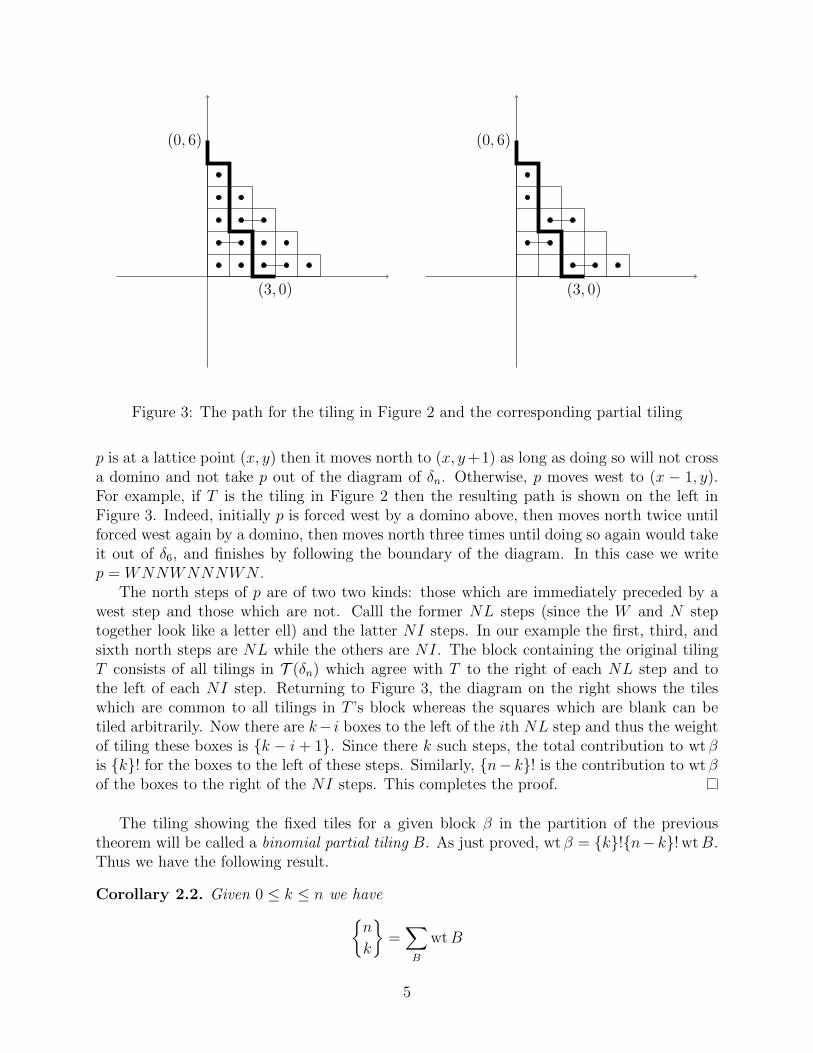
Figure 3: The path for the tiling in Figure 2 and the corresponding partial tiling

p is at a lattice point (x, y) then it moves north to (x, y+1) as long as doing so will not crossa domino and not take p out of the diagram of δn. Otherwise, p moves west to (x − 1, y).For example, if T is the tiling in Figure 2 then the resulting path is shown on the left inFigure 3. Indeed, initially p is forced west by a domino above, then moves north twice untilforced west again by a domino, then moves north three times until doing so again would takeit out of δ6, and finishes by following the boundary of the diagram. In this case we writep = WNNWNNNWN .

The north steps of p are of two two kinds: those which are immediately preceded by awest step and those which are not. Calll the former NL steps (since the W and N steptogether look like a letter ell) and the latter NI steps. In our example the first, third, andsixth north steps are NL while the others are NI. The block containing the original tilingT consists of all tilings in T (δn) which agree with T to the right of each NL step and tothe left of each NI step. Returning to Figure 3, the diagram on the right shows the tileswhich are common to all tilings in T ’s block whereas the squares which are blank can betiled arbitrarily. Now there are k− i boxes to the left of the ith NL step and thus the weightof tiling these boxes is {k − i + 1}. Since there k such steps, the total contribution to wt βis {k}! for the boxes to the left of these steps. Similarly, {n− k}! is the contribution to wt βof the boxes to the right of the NI steps. This completes the proof.

The tiling showing the fixed tiles for a given block β in the partition of the previoustheorem will be called a binomial partial tiling B. As just proved, wt β = {k}!{n− k}! wtB.Thus we have the following result.

Corollary 2.2. Given 0 ≤ k ≤ n we have{n

k

}=∑B

wtB

5

Figure 4: The tiling of a rectangle corresponding to the partial tiling in Figure 3

where the sum is over all binomial partial tilings associated with lattice paths from (k, 0) to(0, n) in δn. Thus

{nk

}∈ N[s, t].

We end this section by describing the relationship between the tilings we have been con-sidering and those in the model of Sagan and Savage. In their interpretation, one consideredall lattice paths p in a k × (n − k) rectangle R starting at the southwest corner, ending atthe northeast corner, and taking unit steps north and east. The path divides R into twopartitions: λ whose parts are the rows of boxes in R northwest of p and λ∗ whose parts arethe columns of R southeast of p. One then considers all tilings of R which are tilings of λ (soany dominoes are horizontal) and of λ∗ (so any dominoes are vertical) such that each tiling ofa column of λ∗ begins with a domino. They then proved that

{nk

}is the generating function

for all such tilings. But there is a bijection between these tilings and our binomial partialtilings where one uses the fixed tilings to left of NI steps for the rows of λ and those to theright of the NL steps for λ∗. Figure 4 shows the tiling of R corresponding to the partialtiling in Figure 3. Note that dominoes in the tiling of λ∗ occur naturally in the context ofbinomial partial tilings rather than just being an imposed condition. And, as we will see,the viewpoint of partial tilings is much more flexible than that of tilings of a rectangle.

3 Identities for Lucasnomials

We will now use Corollary 2.2 to prove various identities for Lucasnomials. We start withthe analogue of the binomial recursion mentioned in the introduction. In the Sagan andSavage paper, this formula was first proved by other means and then used to obtain theircombinatorial interpretation. Here, the recursion follows easily from our model.

Proposition 3.1. For 0 < k < n we have{n

k

}= {k + 1}

{n− 1

k

}+ t{n− k − 1}

{n− 1

k − 1

}.

Proof. By Corollary 2.2 it suffices to partition the set of partial tilings for{nk

}into two

subsets whose generating functions give the two terms of the recursion. First consider thebinomial partial tilings B whose path p starts from (k, 0) with an N step. Since this is anNI step, the portion of the first row to the left of the step is tiled, and by Proposition 1.1the generating function for such tilings is {k + 1}. Now p continues from (k, 1) through theremaining rows which form the partition δn−1. It follows that the weights of this portionof the corresponding partial tilings sum to

{n−1k

}. Thus these p give the first term of the

recursion.

6

1 2 3 4 5 6 7

1

2

3

4

5

6

7

B

S1

S2

Figure 5: An extended binomial partial tiling of type (7, 5, 2)

Suppose now that p starts with a W step. It follows that the second step of p must beN and so an NL step. In this case the portion of the first row to the right of the NL stepis tiled and that tiling begins with a domino. Using the same reasoning as in the previousparagraph, one sees that the weight generating function for the tiling of the first row ist{n− k − 1} while

{n−1k−1

}accounts for the rest of the rows of the tiling.

We will next give a bijective proof of the symmetry of the Lucasnomials. In particular,we will construct an involution to demonstrate the following result.

Proposition 3.2. For 0 ≤ t ≤ k ≤ n we have

{k}{k − 1} . . . {k − t+ 1}{n

k

}= {n− k + t} . . . {n− k + 1}

{n

n− k + t

}. (2)

In particular, when t = 0, {n

k

}=

{n

n− k

}.

Although this proposition is easy to prove algebraically, the algorithm giving the invo-lution is surprisingly intricate. To define the bijection we will need the following concepts.A strip of length k will be a row of k squares, that is, the Young diagram of λ = (k).For 0 ≤ t ≤ k ≤ n an extended binomial partial tiling of type (n, k, t) is a (t + 1)-tupleB = (B;S1, . . . , St) where

1. B is a partial binomial tiling of δn whose lattice path starts at (k, 0), and

2. Si is a tiled strip of length k − i for 1 ≤ i ≤ t.

For brevity we will sometimes write B = (B;S) where S = (S1, . . . , St). In figures, we willdisplay the strips to the northeast of B. See Figure 5 for an example with (n, k, t) = (7, 5, 2).Clearly the sum of the weights of all B of type (n, k, t) is the left-hand side of equation (2).Our involution will be a map ι : B 7→ C where B and C are of types (n, k, t) and (n, n−k+t, t),respectively. This will provide a combinatorial proof of Proposition 3.2.

7

To describe the algorithm producing ι we need certain operations on partial binomialtilings and strips. Given two strips R, S we denote their concatenation by RS or R · S. So,using the strips in Figure 5,

S1S2 = S1 · S2 = .

Given a partially tiled strip R of length n and a partial binomial tiling B of δn we definetheir concatenation, RB = R ·B, to be the tiling of δn+1 whose first (bottom) row is R andwith the remaining rows tiled as in B. So if B′ is the partial tiling of δ6 given by the top sixrows of the partial tiling B in Figure 5 then B = RB′ where

R = .

Note that only for certain R will the concatenation RB remain a partial binomial tiling forsome path. In particular R will have to be either a left strip where only the left-most boxesare tiled, or a right strip with tiles only on the right-most boxes. The example R is a rightstrip tiled by a domino.

Given a strip S of length k and 0 ≤ s ≤ k we define Sbsc and Sdse to be the stripsconsisting of, respectively, the first s and the last s boxes of S. Continuing our example

S1b3c = and S1d3e = .

Note that these notations are undefined if taking the desired boxes would involve breakinga domino. Also, to simplify notation, we will use RSbsc to be the first s boxes of theconcatentation of RS, while R ·Sbsc will be the concatenation of R with the first s boxes ofS. A similar convention applies to the last s boxes. We will also use the notation Sr for thereverse of a strip obtained by reflecting it in a vertical axis. In our example,

Sr2 = .

Our algorithm will break into four cases depending on the following concept. Call a point(r, 0) an NI point of a partial binomial tiling B if taking an N step from this vertex staysin B and does not cross a domino. Otherwise call (r, 0) an NL point which also includes thecase where this vertex is not in B to begin with. We consider use the previous two definitionsfor strips by considering them as being embedded in the first quadrant as a one-row partition.Because our algorithm is recursive, we will have to be careful about its notation. A priori,given a partial binomial tiling B the notation ι(B) is not well defined since ι needs as inputa pair B = (B;S). However, it will be convenient to write

ι(B;S1, . . . , St) = (ι(B); ι(S1), . . . , ι(St))

where it is understood on the right-hand side that ι is always taken with respect to the inputpair (B;S) to the algorithm. Because the algorithm is recursive, we will also have to applyι to B′ = (B′;S ′1, . . . , S

′r) where B′ is B with its bottom row removed and S ′1, . . . , S

′r are

certain strips. So we define ι′(B′) and ι′(S ′i) for 1 ≤ i ≤ r by

ι(B′;S ′1, . . . , S′r) = (ι′(B′); ι′(S ′1), . . . , ι

′(S ′r)).

8

Algorithm ι

Input: An extended binomial tiling B = (B;S1, . . . , St) having type (n, k, t).

Output: An extended binomial tiling ι(B) = (C;T1, . . . , Tt) = (C; T ) having type(n, n− k + t, t).

1. If n = 0 then ι is the identity and C = B.

2. If n > 0 then let R be the strip of tiled squares in the bottom row of B, and let B′ beB with the bottom row removed.

3. Construct B′ = (B′,S ′), calculate ι′(B′) recusively, and then define ι(B) using thefollowing four cases.

(a) If (k, 0) is an NI point of B and (k − t− 1, 0) is an NI point of B then let

St+1 = Rbk − t− 1c,S ′ = (S1, . . . , St, St+1),C = RL · ι′(B′) where RL is a left strip tiled by R′ = ι′(St+1) ·Rdt+ 1er,T = (ι′(S1), . . . , ι

′(St)).

(b) If (k, 0) is an NI point of B and (k − t− 1, 0) is an NL point of B then let

S ′ = (S1, . . . , St),C = RR · ι′(B′) where RR is a right strip tiled by R′ = Rbk − tcr,T = (ι′(St) ·Rdter, ι′(S1), . . . , ι

′(St−1)).

(c) If (k, 0) is an NL point of B and (k− t−1, 0) is an NI point of S1 (by convention,this is considered to be true if t = 0 so that S1 does not exist) then let

St+1 = S1bk − t− 1c,S ′ = (S2, . . . , St, St+1),C = RL · ι′(B′) where RL is a left strip tiled by R′ = RrSr

1bn− k + tc,T = (ι′(S2), . . . , ι

′(St), ι′(St+1)).

(d) If (k, 0) is an NL point of B and (k − t− 1, 0) is an NL point of S1 then let

S ′ = (S2, . . . , St),C = RR · ι′(B′) where RR is a right strip tiled by R′ = RrSr

1dk − te,T = (RrSr

1bn− k + t− 1c, ι′(S2), . . . , ι′(St)).

Figure 6: The algorithm for computing the involution ι

9

In particular, if S ′i = Sj for some i, j then ι′(Sj) = ι′(S ′i) so that Sj is being treated asan element of B′ rather than of B. We now have all the necessary concepts to present therecursive algorithm which is given in Figure 6.

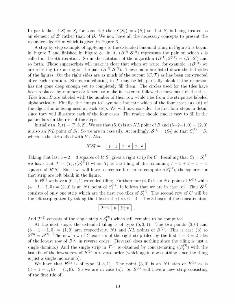
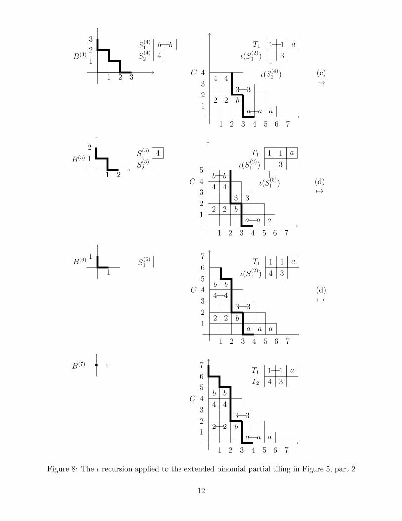
A step-by-step example of applying ι to the extended binomial tiling in Figure 5 is begunin Figure 7 and finished in Figure 8. In it, (B(i);S(i)) represents the pair on which ι iscalled in the ith iteration. So in the notation of the algorithm (B(1);S(1)) = (B′;S ′) andso forth. These superscripts will make it clear that when we write, for example, ι(B(i)) weare referring to ι acting on the pair (B(i);S(i)). These pairs are listed down the left sidesof the figures. On the right sides are as much of the output (C, T ) as has been constructedafter each iteration. Strips contributing to T may be left partially blank if the recursionhas not gone deep enough yet to completely fill them. The circles used for the tiles havebeen replaced by numbers or letters to make it easier to follow the movement of the tiles.Tiles from B are labeled with the number of their row while tiles from the strips are labeledalphabetically. Finally, the “maps to” symbols indicate which of the four cases (a)–(d) ofthe algorithm is being used at each step. We will now consider the first four steps in detailsince they will illustrate each of the four cases. The reader should find it easy to fill in theparticulars for the rest of the steps.

Initially (n, k, t) = (7, 5, 2). We see that (5, 0) is anNL point ofB and (5−2−1, 0) = (2, 0)

is also an NL point of S1. So we are in case (d). Accordingly, S(1) = (S2) so that S(1)1 = S2

which is the strip filled with b’s. Also

1 1 a a a aRrSr1 = .

Taking that last 5− 2 = 3 squares of RrSr1 gives a right strip for C. Recalling that S2 = S

(1)1

we have that T = (T1, ι(S(1)1 )) where T1 is the tiling of the remaining 7 − 5 + 2 − 1 = 3

squares of RrSr1 . Since we will have to recurse further to compute ι(S

(1)1 ), the squares for

that strip are left blank in the figure.In B(1) we have a (6, 4, 1) extended tiling. Furthermore (4, 0) is an NL point of B(1) while

(4 − 1 − 1, 0) = (2, 0) is an NI point of S(1)1 . It follows that we are in case (c). Thus S(2)

consists of only one strip which are the first two tiles of S(1)1 . The second row of C will be

the left strip gotten by taking the tiles in the first 6− 4− 1 = 3 boxes of the concatenation

2 2 b b b .

And T (2) consists of the single strip ι(S(2)1 ) which still remains to be computed.

At the next stage, the extended tiling is of type (5, 3, 1). The two points (3, 0) and(3 − 1 − 1, 0) = (1, 0) are, respectively, NI and NL points of B(2). This is case (b) soS(3) = S(2). The new row of C consists of the right strip tiled by the first 5 − 3 = 2 tilesof the lowest row of B(2) in reverse order. (Reversal does nothing since the tiling is just a

single domino.) And the single strip in T (3) is obtained by concatenating ι(S(3)1 ) with the

last tile of the lowest row of B(2) in reverse order (which again does nothing since the tilingis just a single monomino).

We have that B(3) is of type (4, 3, 1). The point (3, 0) is an NI step of B(3) as is(3 − 1 − 1, 0) = (1, 0). So we are in case (a). So S(4) will have a new strip consistingof the first tile of

10

1 2 3 4 5 6 7

1

2

3

4

5

6

7

1 1

2 2

3 3 3

4 4 4

a a a a

b b b

B

S1

S2

(C, T ) = ∅ (d)7→

1 2 3 4 5 6

1

2

3

4

5

6

2 2

3 3 3

4 4 4

b b b

B(1)

S(1)1

C

1

1 2 3 4 5 6 7

a a a

1 1 aT1

ι(S(1)1 )

(c)7→

B(2)

1 2 3 4 5

1

2

3

4

5

3 3 3

4 4 4

b bS(2)1

C

1

2

1 2 3 4 5 6 7

a a a

2 2 b

1 1 aT1

ι(S(2)1 )

(b)7→

B(3)

1 2 3 4

1

2

3

4

4 4 4

b bS(3)1

C

1

2

3

1 2 3 4 5 6 7

a a a

2 2 b

3 3

1 1 a

3

T1

ι(S(2)1 )

ι(S(3)1 ) (a)

7→

Figure 7: The ι recursion applied to the extended binomial partial tiling in Figure 5, part 1

11

B(4)

1 2 3

1

2

3b b

4

S(4)1

S(4)2

C

1

2

3

4

1 2 3 4 5 6 7

a a a

2 2 b

3 3

4 4

1 1 a

3

T1

ι(S(2)1 )

ι(S(4)1 ) (c)

7→

B(5)

1 2

1

24S

(5)1

S(5)2

C

1

2

3

4

5

1 2 3 4 5 6 7

a a a

2 2 b

3 3

4 4

b b

1 1 a

3

T1

ι(S(2)1 )

ι(S(5)1 ) (d)

7→

B(6)

1

1S(6)1

C

1

2

3

4

5

6

7

1 2 3 4 5 6 7

a a a

2 2 b

3 3

4 4

b b

1 1 a

34

T1

ι(S(2)1 )

(d)7→

B(7)

C

1

2

3

4

5

6

7

1 2 3 4 5 6 7

a a a

2 2 b

3 3

4 4

b b

1 1 a

34

T1

T2

Figure 8: The ι recursion applied to the extended binomial partial tiling in Figure 5, part 2

12

4 4 4 .

Now C adds a row consisting of the reversal of the tiles on the remaining two squares of theabove strip, while T does not change from the previous step.

Theorem 3.3. The map ι is a well defined involution on extended binomial tilings.

Proof. We induct on n where the case n = 0 is trivial. So assume n > 0 and that the theoremholds for extended binomial tilings with first parameter n− 1. We will now go through eachof the cases of the algorithm in turn.

Consider case (a). To check that ι is well defined, we must first show that restricting tothe first k−t−1 (or the last t+1) boxes of R does not break a domino. But this is true sinceR has length k and (k− t− 1, 0) is an NI point of B. Note also that |St+1| = k− t− 1 is thecorrect length to be the final strip in S ′ since one takes an NI step to go from B to B′ andso the path still has x-coordinate k. Similarly, the other strips of S ′ have the appropriatelengths. Next we must be sure that the left strip used for the bottom of C will permit thebeginning of a path starting at (n − k + t, 0) with an NI step. First note that the formsof B′ and S ′ show that B′ has parameters (n − 1, k, t + 1), so by induction ι′(B′) has type(n− 1, n− k + t, t+ 1) It follows that ι′(St+1) has length (n− k + t)− (t+ 1) = n− k − 1,and the number of boxes tiled in the first row of C is

|ι′(St+1) ·Rdt+ 1er| = (n− k − 1) + (t+ 1) = n− k + t

as desired. We must also make sure that once the NI step is taken in C, its end point willbe the same as the initial point of the path when we compute ι′(B′). But since the firststep in C will be NI, its x-coordinate will still be n − k + t which agrees with the middleparameter computed for ι′(B′) above. Finally, we must check that the entries of T have thecorrect lengths. But this follows from the fact that the middle parameters for B and B′ areboth k.

We now check that ι2(B) = B in case (a). To avoid confusion we will always use twodifferent alphabets to distinguish between B and C = ι(B). So, for example Si will always bethe ith strip of B, not the ith strip of C which will be denoted Ti. In the previous paragraphwe saw that C starts with an NI step. Furthermore, the definition of R′ as a concatenationshows that (k − t− 1, 0) is an NI point of C. So C is again in case (a). By induction ι′(B′)will be B with its lowest row removed. And the bottom row will be a left strip tiled by

(ι′)2(St+1) ·R′dt+ 1er = St+1 ·Rdt+ 1e = Rbk − t− 1c ·Rdt+ 1e = R.

Thus ι2(B) = B. Also, using induction,

ι2(S) = ι′(T ) = ((ι′)2(S1), . . . , (ι′)2(St)) = S.

Hence ι2(B) = B as we wished to prove.For the remaining three cases, much of the demonstration of being well defined is similar

to what was done in case (a). So we will just mention any important points of difference. Incase (b), the fact that (k−t−1, 0) is an NL point for B implies that there is a domino betweensquares k− t− 1 and k− t in the bottom row of B. In particular, this means that (k− t, 0)

13

is an NI point for B and so it is possible to take the first k − t squares of R when formingR′. Note also that by definition of the right strip RR, the domino just mentioned will coversquares n−k+t and n−k+t+1 in the bottom row of C. Thus a path starting at (n−k+t, 0)will be forced west and so this will an NL point of C. Furthermore, the first component ofT is ι′(St) ·Rdter, where by induction ι′(St) has length [(n− 1)− k + t]− t = n− k − 1. Sothis gives an NI point of T1 with coordinates (n − k − 1, 0) = ((n − k + t) − t − 1, 0) andthus C is in case (c).

To see that we have an involution in case (b), we have just noted that for B in this casewe have C = ι(B) is in case (c). As usual, ι′(B′) returns the top rows of B to what theywere. As for the bottom row we have, by definition of case (c) and the fact that C is of type(n, n− k + t, t), that it is a left strip tiled by

(R′)rT r1 bn− (n− k + t)− tc = (Rbk − tc)(Rdte · ι′(St)

r)bkc = R.

Finally, we have

ι2(S) = (ι′(T2), . . . , ι′(Tt+1)) = ((ι′)2(S1), . . . , (ι

′)2(St−1), ι′(T1b(n− k + t)− t− 1c))

whereT1b(n− k + t)− t− 1c = (ι′(St) ·Rdter)bn− k − 1c = ι′(St).

So by induction ι2(S) = S in this case as well.The proof if B is in case (c) is similar to the one for case (b) which is its inverse so this

part of the demonstration will be omitted. Finally we turn to case (d). To prove that thiscase is well defined, one again checks that the dominoes which force (k, 0) to be an NL pointof B and (k − t − 1, 0) to be an NL point of S1 appear in T1 and C, respectively, so that((n− k+ t)− t− 1, 0) = (n− k− 1, 0) is an NL point of T1 and (n− k+ t, 0) is an NL pointof C. One then uses this fact to show that applying ι twice is the identity. But no new ideasappear so we will leave these details to the reader.

4 Catalan and Fuss-Catalan numbers

The well-known Catalan numbers are given by

Cn =1

n+ 1

(2n

n

)for n ≥ 0. So the Lucas analogue is

C{n} =1

{n+ 1}

{2n

n

}.

In 2010, Lou Shapiro suggested this definition. Further, he asked whether this was a poly-nomial in s and t and, if so, whether it had a combinatorial interpretation. There is asimple relation between C{n} and the Lucasnomials which shows that the answer to the firstquestion is yes. This was first pointed out by Shalosh Ekhad [Ekh11]. We will prove thisequation combinatoriallly below. We can now show that the second question also has anaffirmative answer.

14

(2, 0)

(0, 6)

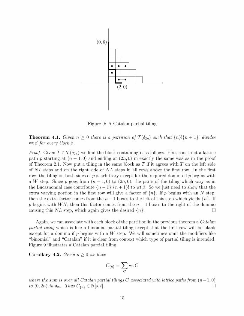
Figure 9: A Catalan partial tiling

Theorem 4.1. Given n ≥ 0 there is a partition of T (δ2n) such that {n}!{n + 1}! divideswt β for every block β.

Proof. Given T ∈ T (δ2n) we find the block containing it as follows. First construct a latticepath p starting at (n − 1, 0) and ending at (2n, 0) in exactly the same was as in the proofof Theorem 2.1. Now put a tiling in the same block as T if it agrees with T on the left sideof NI steps and on the right side of NL steps in all rows above the first row. In the firstrow, the tiling on both sides of p is arbitrary except for the required domino if p begins witha W step. Since p goes from (n − 1, 0) to (2n, 0), the parts of the tiling which vary as inthe Lucasnomial case contribute {n− 1}!{n+ 1}! to wt β. So we just need to show that theextra varying portion in the first row will give a factor of {n}. If p begins with an N step,then the extra factor comes from the n− 1 boxes to the left of this step which yields {n}. Ifp begins with WN , then this factor comes from the n− 1 boxes to the right of the dominocausing this NL step, which again gives the desired {n}.

Again, we can associate with each block of the partition in the previous theorem a Catalanpartial tiling which is like a binomial partial tiling except that the first row will be blankexcept for a domino if p begins with a W step. We will sometimes omit the modifiers like“binomial” and “Catalan” if it is clear from context which type of partial tiling is intended.Figure 9 illustrates a Catalan partial tiling

Corollary 4.2. Given n ≥ 0 we have

C{n} =∑C

wtC

where the sum is over all Catalan partial tilings C associated with lattice paths from (n−1, 0)to (0, 2n) in δ2n. Thus C{n} ∈ N[s, t].

15

We can now give a combinatorial proof of the identity relating the Lucas-Catalan poly-nomials C{n} and the Lucasnomials which we mentioned earlier.

Proposition 4.3. For n ≥ 2 we have

C{n} =

{2n− 1

n− 1

}+ t

{2n− 1

n− 2

}.

Proof. By Corollary 4.2, it suffices to partition the Catalan partial tilings P into two subsetswhose weight generating functions are the two terms in the sum. First consider the partialtilings associated with lattice paths p whose first step is N . Then the bottom row of P isblank. And the portion of p in the remaining rows goes from (n−1, 1) to (0, 2n) inside δ2n−1.Thus the contribution of these partial tilings is

{2n−1n−1

}. If instead p begins with WN , then

there is a single domino in the first row which contributes t. The rest of the path goes from(n− 2, 1) to (0, 2n) inside δ2n−1 and so contributes

{2n−1n−2

}as desired.

Note that this proposition is a Lucas analogue of the well-known identity

Cn =

(2n− 1

n− 1

)−(

2n− 1

n− 2

)obtained when s = 2 and t = −1.

We now wish to study the Lucas analogue of the Fuss-Catalan numbers which are

Cn,k =1

kn+ 1

((k + 1)n

n

)for n ≥ 0 and k ≥ 1. Clearly Cn,1 = Cn. Consider the Lucas analogue

C{n,k} =1

{kn+ 1}

{(k + 1)n

n

}.

To prove the next result, it will be convenient to give coordinates to the squares of aYoung diagram λ. We will use brackets for these coordinates to distinguish them from theCartesian coordinates we have been using for lattice paths. Let [i, j] denote the square inrow i from the bottom and column j from the left. Alternatively, if a square has northeastcorner with Cartesian coordinates (j, i) then the square’s coordinates are [i, j].

Theorem 4.4. Given n ≥ 0, k ≥ 1 there is a partition of T (δ(k+1)n) such that {n}!{kn+ 1}!divides wt β for every block β.

Proof. To find the block containing a tiling T of δ(k+1)n we proceed as follows. Consider theusual lattice path p in T starting at (n − 1, 0) and ending at ((k + 1)n, 0). If p starts withan N step, then we construct β exactly as in the proof of Theorem 4.1. In this case, theparts of the tiling which vary as in the Lucasnomial case contribute {n− 1}!{kn + 1}! andthe squares in the first row to the left of the NI step give a factor of {n} so we are done forsuch paths.

Now suppose p beginsWN . It follows that there is a domino of T between squares [1, n−1]and [1, n]. Also, there is no domino between squares [1, (k+1)n−1] and [1, (k+1)n] because

16

(2, 0)

(0, 9)

Figure 10: A Fuss-Catalan partial tiling

the latter square is not part of δ(k+1)n. So there is a smallest index m such that there isa domino between [1,mn − 1] and [1,mn] but no domino between [1, (m + 1)n − 1] and[1, (m + 1)n]. The block of β will consist of all tilings agreeing with T as for Lucasnomialsin rows above the first. And in the first row they agree with T to the right of the NL stepexcept in the squares from [1,mn + 1] through [1, (m + 1)n− 1] where the tiling is allowedto vary. As in the previous paragraph, the variable parts of β which are the same as forLucasnomials contribute {n− 1}!{kn+ 1}! while the variable portion to the right of the firstNL gives a factor of {n}. This finishes the demonstration.

As usual, we can represent a block β of this partition by a Fuss-Catalan partial tiling.Figure 10 displays such a tiling when n = 3, k = 2, and m = 2 (in the notation of theprevious proof).

Corollary 4.5. Given n ≥ 0, k ≥ 1 we have

C{n,k} =∑P

wtP

where the sum is over all Fuss-Catalan partial tilings associated with lattice paths going from(n− 1, 0) to (0, (k + 1)n) in δ(k+1)n. Thus C{n,k} ∈ N[s, t].

The next result is proved in much the same way as Proposition 4.3 and so the demon-stration is left to the reader.

Proposition 4.6. For n ≥ 2, k ≥ 1 we have

C{n,k} =

{(k + 1)n− 1

n− 1

}+

k∑m=1

tm{n}m−1{k −m+ 1}{

(k + 1)n− 1

n− 2

}.

17

W d1, . . . , dn hAn 2, 3, 4, . . . , n+ 1 n+ 1Bn 2, 4, 6, . . . , 2n 2nDn 2, 4, 6, . . . , 2(n− 1), n 2(n− 1) (for n ≥ 3)I2(m) 2,m m (for m ≥ 2)H3 2, 6, 10 10H4 2, 12, 20, 30 30F4 2, 6, 8, 12 12E6 2, 5, 6, 8, 9, 12 12E7 2, 6, 8, 10, 12, 14, 18 18E8 2, 8, 12, 14, 18, 20, 24, 30 30

Figure 11: finite irreducible Coxeter group degrees

5 Coxeter groups and d-divisible diagrams

There is a way to associate a Catalan number and Fuss-Catalan numbers with any finiteirreducible Coxeter group W . This has lead to the area of reseach called Catalan combina-torics. For more details, see the memoir of Armstrong [Arm09]. The purpose of this sectionis to prove that for any W , the Coxeter-Catalan number is in N[s, t]. In fact, we will provemore general results using d-divisible Young diagrams. This will also permit us to prove thatfor the infinite families of Coxeter groups, the Lucas-Fuss-Catalan analogue is in N[s, t].

The finite Coxeter groups W are those which can be generated by reflections. Thosewhich are irreducible have a well-known classification with four infinite families (An, Bn,Dn, and I2(m)) as well as 6 exceptional groups (H3, H4, F4, E6, E7, and E8) where thesubscript denotes the dimension n of the space on which the group acts. Associated witheach finite irreducilble group is a set of degrees which are the degrees d1, . . . , dn of certainpolynomial invariants of the group. The degrees of the various groups are listed in Figure 11.The Coxeter number of W is the largest degree and is denoted h. One can now define theCoxeter-Catalan number of W to be

CatW =n∏

i=1

h+ didi

with corresponding Lucas-Coxeter analogue

Cat{W} =n∏

i=1

{h+ di}{di}

.

If W is of type Jn for some J then we will also use the notation J{n} for {W}. Directly fromthe definitions, CatAn−1 = Cn. Also, after cancelling powers of 2, we have CatBn =

(2nn

).

But {2n} 6= {2}{n} so we will have to find another way to deal with CatB{n}. In fact, wewill be able to give a combinatorial interpretation when the numerator and denominator areboth constructed using “Lucastorials” containing the integers divisible by some fixed integerd ≥ 1.

18

Define the d-divisible Lucastorial as

{n : d}! = {d}{2d} . . . {nd}

with corresponding d-divisible Lucasnomial{n : d

k : d

}=

{n : d}!{k : d}!{n− k : d}!

for 0 ≤ k ≤ n. So we have

CatB{n} =

{2n : 2

n : 2

}.

Also define the d-divisible staircase parttion

δn:d = (nd− 1, (n− 1)d− 1, . . . , 2d− 1, d− 1).

The fact that wt δn:d = {n : d}! follows immediately from the definitions.

Theorem 5.1. Given d ≥ 1 and 0 ≤ k ≤ n there is a partition of T (δn:d) such that{k : d}!{n− k : d}! divides wt β for every block β.

Proof. We determine the block β containing a tiling T by constructing a path p from (kd, 0)to (0, n) as follows. The path takes an N step if and only if three conditions are satisfied:the two for Lucasnomial paths (the step does not cross a domino and stays within theYoung diagram) together with the requirement that the x-coordinate of the N step must becongruent to 0 or −1 modulo d with at most one N step on each line of the latter type. Sop starts by either goes north along x = kd or, if there is a blocking domino, taking a W stepand going north along x = kd−1. In the first case it can take another N step if not blocked,or go W and then N if it is. In the second case, p proceeds using W steps to ((k − 1)d, 1)and either goes north from that lattice point or, if blocked, takes one more W step to gonorth from ((k − 1)d− 1, 1), etc. See Figure 12 for an example. Call an N step an NI stepif it has x-coordinate divisible by d and an NL step otherwise. We now construct β as forLucasnomials: agreeing with T to the left of NI steps and to the right of NL steps. It is aneasy matter to check that {k : d}!{n− k : d}! is a factor of wt β.

The definition of d-divisible partial tiling (illustrated in Figure 12) and the next resultare as expected.

Corollary 5.2. Given d ≥ 1 and 0 ≤ k ≤ n we have{n : d

k : d

}=∑P

wtP

where the sum is over all d-divisible partial tilings associated with lattice paths going from(kd, 0) to (0, n) in δn:d. Thus

{n:dk:d

}∈ N[s, t].

19

(4, 0)

(0, 4)

(4, 0)

(0, 4)

Figure 12: A 2-divisible path on the left and corresponding partial tiling on the right

The Lucas-Coxeter analogue for Dn is

CatD{n} ={3n− 2}{n}

{2(n− 1) : 2

n− 1 : 2

}. (3)

Again, we will be able to prove a d-divisible generalization of this result. But first we need aresult of Hoggatt and Long [HL74] about the divisibility of polynonials in the Lucas sequence.(In their paper they only prove the divisbility statement, but the fact that the quotient is inN[s, t] follows easily from their demonstration.)

Theorem 5.3 ([HL74]). For positive integers m,n we have m divides n if and only if {m}divides {n}. In this case {m}/{n} ∈ N[s, t]. .

If λ, µ are Young diagrams with µ ⊆ λ, then the corresponding skew diagram, λ/µ,consists of all the boxes in λ but not in µ. The skew diagram used in Figure 13 is δ9:2/(5).We will use skew diagrams to prove the following result which yields (3) as a special case.

Theorem 5.4. Given d ≥ 1 we have

{(d+ 1)n− d}{n}

{2(n− 1) : d

n− 1 : d

}(4)

is in N[s, t].

Proof. Tile the rows of the skew shape δ2n−1:d/(d−1)n. It is easy to see that the correspond-ing generating function is the numerator of equation (4) where the bottom row contributes{(2n− 1)d− (d− 1)n} = {(d+ 1)n− d} which is the numerator of the fractional factor. Asusual, we group the tilings into blocks β and show that the denominator of (4) divides theweight of each block. Given a tiling T we find its block by starting a lattice path p at (nd, 0)and using exactly the same rules as in the proof of Theorem 5.1. See the upper diagram inFigure 13 for an example when d = 2 and n = 5. We now let the strips to the side of eachnorth step either be fixed or vary, again as dictated in Theorem 5.1’s demonstration. Thebottom diagram in Figure 13 shows the partial tiling corresponding to the upper diagram.There are two cases.

20

(10, 0)

(0, 9)

(10, 0)

(0, 9)

Figure 13: A lattice path and partial tiling for D{5}

If p starts with an N step then its right side contributes {(2n− 1)d− nd} = {(n− 1)d}.Now p enters the top 2n − 2 rows which form a δ2n−2:d at x-coordinate nd. It follows thatthe contribution of this portion of p to wt β is {n : d}!{n− 2 : d}!. So the total contributionto the weight of the variable parts of each row is

{(n− 1)d} · {n : d}!{n− 2 : d}! = {nd} · {n− 1 : d}!{n− 1 : d}!.

Thanks to Theorem 5.3, this is divisible by {n} · {n − 1 : d}!{n − 1 : d}! which is thedenominator of (4) so we are done with this case.

If p starts with WN , then the left side of p gives a contribution of {nd−n(d−1)} = {n}.Because of the rule that p can take at most one step on a vertical line of the form = kd−1, thepath must now continue to take west steps until it reaches ((n−1)d, 1). Now it can enter theupper rows of the diagram from this point contributing a factor of {n− 1 : d}!{n− 1 : d}! towt β. Multiplying the two contributions gives exactly the denominator of (4) which finishesthis case and the proof.

21

We note that replacing n by n+ 1 in equation (4) we obtain

{(d+ 1)n+ 1}{n+ 1}

{2n : d

n : d

}which, for d = 1, is just a multiple of the nth Lucas-Catalan polynomial. We also note thatone can generalize even further. Given positive integers satisfying l < kd < md, we considerstarting lattice paths from (kdn, 0) in the skew diagram δm(n−1)+1:d/(ld) using the same rulesas in the previous two proofs. This yields the following result whose demonstration is similarenough to those just given that we omit it. But note that we get the previous theorem asthe special case l = d− 1, k = 1, and m = 2.

Theorem 5.5. Given positive integers satisfying l < kd < md we have

{(dm− l)n− (m− 1)d}{gn}

{m(n− 1) : d

kn− 1 : d

}is in N[s, t] where g = gcd(kd, kd− l).

We finally come to our main theorem for this section.

Theorem 5.6. If W is a finite irreducible Coxeter group W then Cat{W} ∈ N[s, t].

Proof. We have already proved the result in types A, B, and D. And for the exceptionalCoxeter groups, we have verified the claim by computer. So we just need to show that

Cat I{2}(m) ={m+ 2}{2m}{2}{m}

is in N[s, t]. But this follows easily from Theorem 5.3. Indeed, if m is odd then the relativelyprime polynomials {2} = s and {m} both divide {2m}. It follows that the same is true oftheir product which completes this case. If m is even then {2} divides {m + 2} and {m}divides {2m}. So, again, we have a polynomial quotient and all quotients have nonnegativeinteger coefficients.

We now turn to the Fuss-Catalan case. For any finite Coxeter group W and positiveinteger k there is a Coxeter-Fuss-Catalan number defined by

Cat(k)W =n∏

i=1

kh+ didi

.

So, there is a corresponding Lucas-Coxeter-Fuss-Catalan analogue given by

Cat(k){W} =n∏

i=1

{kh+ di}{di}

.

In particular, Cat(k)A{n−1} = C{n,k}.

22

Theorem 5.7. If W = An, Bn, Dn, I2(m) then Cat(k){W} ∈ N[s, t].

Proof. We have already shown this for An in Corollary 4.5. For type B we find that

Cat(k)B{n} =n∏

i=1

{2kn+ 2i}{2i}

=

{(k + 1)n : 2

n : 2

}which is a polynomial in s and t with nonnegative coefficients by Corollary 5.2. In the caseof type D we see

Cat(k)D{n} ={2k(n− 1) + n}

{n}

n−1∏i=1

{2k(n− 1) + 2i}{2i}

={(2k + 1)n− 2k}

{n}

{(k + 1)(n− 1) : 2

n− 1 : 2

}which is in N[s, t] by Theorem 5.5.

For Cat(k) I{2}(m) we can use an argument similar to that of the proof of Theorem 5.6.We have that

Cat(k) I{2}(m) ={km+ 2}{(k + 1)m}

{2}{m}and can consider the parity of m and k. If m or k is even then {2} divides {km + 2} and{m} divides {(k + 1)m}. If m and k are both odd then {2} and {m} are relatively primeand both divide {(k + 1)m}. And in all cases the quotients have coefficients in N.

6 Comments and future work

Here we will collect various observations and open problems in the hopes that the readerwill be tempted to continue our work.

6.1 Coefficients

Note that we can write{n} =

∑k

aksn−2k−1tk

where the ak are positive integers and 0 ≤ k ≤ (n − 1)/2. We call a0, a1, . . . the coefficientsequence of {n} and note that any of our Lucas analogues considered previously will alsocorrespond to such a sequence. There are several properties of sequences of real numberswhich are common in combinatorics, algebra, and geometry. One is that the sequence isunimodal which means that there is an index m such that

a0 ≤ a1 ≤ · · · ≤ am ≥ am+1 ≥ . . . .

23

Another is that the sequence is log concave which is defined by the inequality

a2k ≥ ak−1ak+1

for all k, where we assume ak = 0 if the subscript is outside of the range of the sequence.Finally, we can consider the generating function

f(y) =∑k≥0

akyk

and ask for properties of its roots. For more information about such matters, see the surveyarticles of Stanley [Sta89] and Brenti [Bre94]. In particular, the following result is well knownand straightforward to prove.

Proposition 6.1. If a0, a1, . . . is a sequence of positive reals then its generating functionhaving real roots implies that it is log concave. And if the sequence is log concave then it isunimodal.

To see which of these properties are enjoyed by our Lucas analogues, it will be convenientto make a connection with Chebyshev polynomials. The Chebyshev polynomials of the secondkind, Un(x), are defined recursively by U0(x) = 1, U1(x) = 2x, and for n ≥ 2

Un(x) = 2xUn−1(x)− Un−2(x).

It follows immediately that{n} = Un−1(x) (5)

if we set s = 2x and t = −1.

Theorem 6.2. If the Lucas analogue of a quotient of products is a polynomial then it has acoefficient generating function which is real rooted. So if the coefficient sequence consists ofpositive integers then the sequence is log concave and unimodal.

Proof. From the previous proposition, it suffices to prove the first statement. It is well knownand easy to prove by using angle addition formulas that

Un(cos θ) =sin(n+ 1)θ

sin θ.

It follows that the roots of Un(x) are

x = coskπ

n+ 1

for 0 < k < n+ 1 and so real.By equation 5 we see that {n} and Un−1(x/2) have the same coefficient sequence except

that in the former all coefficients are positive and in the latter signs alternate. Now if wetake a quotient of products of the {n} which is a polynomial p(s, t), then the correspondingquotient of products where {n} is replaced by Un−1(x/2) will be a polynomial q(x). Further,from the paragraph above, q(x) will have real roots. It follows that the coefficient sequenceof p(s, t) (which is obtained from q(x) by removing zeros and making all coefficients positive)has a generating function with only real roots.

24

6.2 Rational Catalan numbers

Rational Catalan numbers generalize the ordinary Catalans and have many interesting con-nections with Dyck paths, noncrossing partitions, associahedra, cores of integer partitions,parking functions, and Lie theory. Let a, b be positive integers whose greatest commondivisor is (a, b) = 1. Then the associated ratioinal Catalan number is

Cat(a, b) =1

a+ b

(a+ b

a

).

In particular, it is easy to see that Cat(n, n+ 1) = Cn. We note that the the relative primecondition is needed to ensure that Cat(a, b) is an integer. As usual, consider

Cat{a, b} =1

{a+ b}

{a+ b

a

}.

We will now present a proof that Cat{a, b} is a polynomial in s, t which was obtained by theFields Institute Algebraic Combinatorics Group [ABC+15] for the q-Fibonacci analogue andworks equally well in our context. First we need the following lemma.

Lemma 6.3 ([HL74]). We have ({m}, {n}) = {(m,n)}.Theorem 6.4 ([ABC+15]). If (a, b) = 1 then C{a, b} is a polynomial in s, t.

Proof. Consider the quantity

p ={a+ b}!{a− 1}!{b}!

= {a+ b}{a+ b− 1

a− 1

}.

From the second expression for p, it is clearly a polynomial in s and t. Note that {a}divides evenly into p because p/{a} =

{a+ba

}. Similarly, {a+ b} divides p since p/{a+ b} ={

a+b−1a−1

}. But (a, a+ b) = 1 and so, by the lemma, {a}{a+ b} divides into p. It follows that

p/({a}{a+ b}) = C{a, b} is a polynomial in s, t.

Despite this result, we have been unable to find a combinatorial interpretation for C{a, b}or prove that its coefficients are nonnegative integers, although this has been checked bycomputer for a, b ≤ 50.

6.3 Narayana numbers.

For 1 ≤ k ≤ n we define the Narayana number

Nn,k =1

n

(n

k

)(n

k − 1

).

It is natural to consider the Narayana numbers in this context because Cn =∑

kNn,k.Further discussion of Narayana numbers can be found in the paper of Branden [Bra04]. Inour usual manner, let

N{n,k} =1

{n}

{n

k

}{n

k − 1

}.

Conjecture 6.5. For all 1 ≤ k ≤ n we have N{n,k} ∈ N[s, t].

This conjecture has been checked by computer for n ≤ 100. One could also considerNarayana numbers for other Coxeter groups.

25

6.4 Coxeter groups again

As is often true in the literature on Coxeter groups, our proof of Theorem 5.6 is case bycase. It would be even better if a case-free demonstration could be found. One could alsohope for a closer connection between the geometric or algebraic properties of Coxeter groupsand our combinatorial constructions. Alternatively, it would be quite interesting to give aproof of Theorem 5.6 by weighting one of the standard objects counted by CatW such asW -noncrossing partitions.

Acknowledgment. We had helpful discussions with Nantel Bergeron, Cesar Ceballos,and Volker Strehl about this work.

References

[ABC+15] Farid Aliniaeifard, Nantel Bergeron, Cesar Ceballos, Tom Denton, and Shu XiaoLi. Algebraic Combinatorics Seminar, Fields Institute. 2013–2015.

[Arm09] Drew Armstrong. Generalized noncrossing partitions and combinatorics of Cox-eter groups. Mem. Amer. Math. Soc., 202(949):x+159, 2009.

[BP09] Arthur T. Benjamin and Sean S. Plott. A combinatorial approach to Fibonomialcoefficients. Fibonacci Quart., 46/47(1):7–9, 2008/09.

[Bra04] Petter Branden. q-Narayana numbers and the flag h-vector of J(2×n). DiscreteMath., 281(1-3):67–81, 2004.

[Bre94] Francesco Brenti. Log-concave and unimodal sequences in algebra, combinatorics,and geometry: an update. In Jerusalem combinatorics ’93, volume 178 of Con-temp. Math., pages 71–89. Amer. Math. Soc., Providence, RI, 1994.

[Ekh11] Shalosh B. Ekhad. The Sagan-Savage Lucas-Catalan polynomials have positivecoefficients. 2011.

[GV85] Ira Gessel and Gerard Viennot. Binomial determinants, paths, and hook lengthformulae. Adv. in Math., 58(3):300–321, 1985.

[HL74] Verner E. Hoggatt, Jr. and Calvin T. Long. Divisibility properties of generalizedFibonacci polynomials. Fibonacci Quart., 12:113–120, 1974.

[SS10] Bruce E. Sagan and Carla D. Savage. Combinatorial interpretations of binomialcoefficient analogues related to Lucas sequences. Integers, 10:A52, 697–703, 2010.

[Sta89] Richard P. Stanley. Log-concave and unimodal sequences in algebra, combina-torics, and geometry. In Graph theory and its applications: East and West (Jinan,1986), volume 576 of Ann. New York Acad. Sci., pages 500–535. New York Acad.Sci., New York, 1989.

26