Journal of

Marine Science and Engineering

Article

Combined Longshore and Cross-Shore Modeling forLow-Energy Embayed Sandy Beaches

Yen Hai Tran 1,2,* , Patrick Marchesiello 3 , Rafael Almar 3 , Duc Tuan Ho 1,2,4, Thong Nguyen 1,2,Duong Hai Thuan 5 and Eric Barthélemy 6,*

Citation: Tran, Y.H.; Marchesiello, P.;

Almar, R.; Ho, D.T.; Nguyen, T.;

Thuan, D.H.; Barthélemy, E.

Combined Longshore and

Cross-Shore Modeling for

Low-Energy Embayed Sandy Beaches.

J. Mar. Sci. Eng. 2021, 9, 979.

https://doi.org/10.3390/jmse9090979

Academic Editor: Celene B. Milanes

Received: 12 August 2021

Accepted: 2 September 2021

Published: 7 September 2021

Publisher’s Note: MDPI stays neutral

with regard to jurisdictional claims in

published maps and institutional affil-

iations.

Copyright: © 2021 by the authors.

Licensee MDPI, Basel, Switzerland.

This article is an open access article

distributed under the terms and

conditions of the Creative Commons

Attribution (CC BY) license (https://

creativecommons.org/licenses/by/

4.0/).

1 Faculty of Civil Engineering, Ho Chi Minh City University of Technology (HCMUT), 268 Ly ThuongKiet Street, District 10, Ho Chi Minh City 700000, Vietnam; hotuanduc@hcmut.edu.vn (D.T.H.);nguyenthong@hcmut.edu.vn (T.N.)

2 Vietnam National University Ho Chi Minh City (VNU-HCM), Linh Trung Ward, Thu Duc District,Ho Chi Minh City 700000, Vietnam

3 Laboratoire d’Etudes en Géophysique et Océanographie Spatiales (LEGOS), Université deToulouse/CNRS/CNES/IRD, 31400 Toulouse, France; patrick.marchesiello@ird.fr (P.M.);rafael.almar@ird.fr (R.A.)

4 Asian Centre for Water Research, Ho Chi Minh City University of Technology (HCMUT), 268 Ly ThuongKiet Street, District 10, Ho Chi Minh City 700000, Vietnam

5 Faculty of Civil Engineering, Thuyloi University, Hanoi 116705, Vietnam; duonghaithuan@tlu.edu.vn6 Laboratoire des Ecoulements Géophysiques et Industriels, Université Grenoble Alpes, CNRS, Grenoble-INP,

38000 Grenoble, France* Correspondence: haiyen.tran@hcmut.edu.vn (Y.H.T.); Eric.Barthelemy@grenoble-inp.fr (E.B.)

Abstract: The present study focuses on the long-term multi-year evolution of the shoreline position ofthe Nha Trang sandy beach. To this end an empirical model which is a combination of longshore andcross-shore models, is used. The Nha Trang beach morphology is driven by a tropical wave climatedominated by seasonal variations and winter monsoon intra-seasonal pulses. The combined modelaccounts for seasonal shoreline evolution, which is primarily attributed to cross-shore dynamics butfails to represent accretion that occurs during the height of summer under low energy conditions. Thereason is in the single equilibrium Dean number Ωeq of the ShoreFor model, one of the components ofthe combined model. This equilibrium Dean number cannot simultaneously account for the evolutionof strong intra-seasonal events (i.e., winter monsoon pulses) and the annual recovery mechanismsassociated with swash transport. By assigning a constant value to Ωeq, when the surf similarityparameter is higher than 3.3 (occurrence of small surging breakers in summer), we strongly improvethe shoreline position prediction. This clearly points to the relevance of a multi-scale approach,although our modified Ωeq retains the advantage of simplicity.

Keywords: shoreline model; one-line model; embayed beach; low-energy beach; cross-shore; longshore

1. Introduction

Empirical data-driven models are increasingly being used for modeling shorelinechanges on time scales from days to decades [1–9]. They are based on a set of parametersrepresenting the contribution of complex physical processes that are evaluated on a calibra-tion period using observed shoreline data. These models are simpler but also much lesscomputationally expensive to simulate long-term shoreline changes than physics-basedmodels such as Delft3D [10], XBeach [11], or Mike21 [12]. These data-driven empiricalmodels essentially apply to natural beaches with no anthropic interference, beaches thatare more or less in equilibrium with the wave forcing conditions.

On one hand, shoreline changes on small time scales for such type of beaches areprimarily attributed to cross-shore transport [7]. The cross-shore empirical models usedfor long-term predictions predominantly assume that a sandy beach tends towards an

J. Mar. Sci. Eng. 2021, 9, 979. https://doi.org/10.3390/jmse9090979 https://www.mdpi.com/journal/jmse

J. Mar. Sci. Eng. 2021, 9, 979 2 of 15

equilibrium for a wave forcing uniform in time [5,13,14]. The shoreline evolution can thusbe represented as a relaxation process towards equilibrium [15,16] that takes the form

∂S∂t

= F(∆Ω) (1)

where S(t) is the shoreline position in the transect; t is time; ∂S∂t is the rate of shoreline

change; Ω is the dimensionless fall velocity (Dean number or Gourlay number): Ω = HwsT ,

a function of H the offshore significant wave height, ws the sediment fall velocity, and Tthe peak wave period; and ∆Ω is called the disequilibrium Dean number, ∆Ω = Ωeq −Ω,where Ωeq represents the equilibrium forcing. The success of cross-shore models relies onthe timescale used to correct the disequilibrium of shoreline position under a particularforcing. To improve its predictive skills, the work in [17] uses a multi-timescale approach,which accounts for storms and seasonal and inter-annual wave climate variability, includingthe scale interactions between these different forcings.

On the other hand, long-term evolution is generally associated with the longshoredrift, i.e., the transport of sediments by wave-driven currents along the coast. In one-linemodels, the littoral drift is the only mechanism of shoreline evolution. The theory in [18] isregarded as a cornerstone of these models, which describes the shoreline evolution due tobeach curvature ∂2S

∂x2 , following a diffusion equation (with κ a diffusion coefficient):

∂S∂t

= κ∂2S∂x2 (2)

Longshore transport can be significant even on a seasonal scale on very curvedcoastlines such as embayed beaches [19]. These shorelines may rotate in time around apivotal point due to changing wave directions. To translate a longshore drift gradient intoa change in the shoreline, it is assumed in one-line models that the beach profile moves ina direction transverse to the coast while maintaining its unchanging shape [2]. A secondassumption is that sand is transported alongshore between the active berm and a closuredepth hc, beyond which the beach is inactive, i.e., there is no erosion or accretion [20].In this case, the shoreline changes with the alongshore gradient of the volumetric longshoretransport rate Qx as

∂S∂t

= − 1hc + B

∂Qx

∂x(3)

where B is the berm height, and Qx is a function of the breaking wave height and long-shore direction, i.e., the longshore wave power, as in the widely used CERC formula [21].There are a number of such models based on various additional features and numericalimplementations [22–25]. A wave sheltering procedure for large wave angles, which trig-gers an instability mechanism generating large-scale morphology over long timescales, isintroduced by [22]. A new vector-based model with more flexible shoreline cell shape issuggested by [23]. The GSb model [9,25] is based on the one-line approach to investigatethe longshore drift at a coastal mound made up of non-cohesive sediments, e.g., sand,gravel, cobbles, shingle, and rock. The ShorelineS model in [24] is the latest model forlong-term shoreline evolution and is capable of simulating rich coastal transformationbehavior of complex shoreline features through its flexible grid.

For a coastline dominated by both cross-shore and longshore transport, as for embayedbeaches, a model that considers both transport processes is expected to improve a skillfulhindcast. An integrated shoreline model considering sea-level rise in addition to cross-shore and longshore transport is developed in [6] . In this model, called CosMos-COAST,the cross-shore contribution to shoreline change is based on the work in [13], the longshorecontribution is based on the one-line concept in [18], and the last contribution is fromthe sea level rise response model in [26]. Other combinations such as that of [7] whocombine the ShoreFor cross-shore model in [5] and a hybrid one-line approach derivedin [22]. Along this line [1] suggested coupling the ShoreFor model with a simpler longshore

J. Mar. Sci. Eng. 2021, 9, 979 3 of 15

model based on a sediment budget and the empirical CERC formula [21]. In the latter, itis assumed that an equilibrium exists in the form of an average shoreline position. Thus,the longshore model variables can be decomposed into a mean and fluctuating contributionin the time series.

In the present study, we will pay particular attention to the suitability of a longshoremodel for embayed beaches and the ability of a single equilibrum cross-shore model torepresent accretion during summer low wave energy conditions. Nha Trang, Vietnam, isan embayed beach with a curved shoreline [27], and thus provides a good test case for thecombined model of [1] that accounts for both cross-shore and longshore contributions. NhaTrang’s climate is characterized by strong seasonal forcing, i.e., summer monsoons withlow-energy waves and winter monsoons with high-energy waves, including intra-seasonalwinter pulses [28,29]. Because shoreline evolution models are typically calibrated with datafrom moderate- to high-energy beaches [5,6], the case of low-energy beaches was neglected,even though, as we will see, they present an additional challenge to these models.

In Section 2, the combined model of the work in [1] is briefly recalled. Section 3describes the characteristics of Nha Trang beach. The result of the combined modelimplemented on the embayed beach shoreline of Nha Trang is presented in Section 4, andSection 5 presents the concluding remarks.

2. Methods

The combined model of Tran and Barthélemy (2020) [1] is built by replacing in theShoreFor model equation of the work in [5] the free parameter d (representing a long-termtrend) with a longshore model equation. The combined model is written as

∂S∂t

= c(

F+ + rF−)+ H3/2

b[a cos2αb

′ + b sin2αb′] (4)

where t is time in days; S(t) is the shoreline position; and F+ and F− represent the accretionand erosion forcing terms, respectively [5]. The parameter r is called the erosion ratio [5].The forcing term F is the product of the incident wave power P and the disequilibriumDean number ∆Ω [5]. ∆Ω is defined by ∆Ω(t) = Ω(t)−Ωeq(t). Ω(t) is the instantaneousDean number. Ωeq(t) is the equilibrium Dean number which is defined by [14,16]

Ωeq(t) =∑

2φ∆tj=1 Ωj10−j∆t/φ

∑2φ∆tj=1 10−j∆t/φ

(5)

where φ (day) is the “memory decay”, ∆t is the wave forcing data time step, and j is thenumber of data points in the survey time series prior to the calculation point at time t [14].

In Equation (4), a, b, and c (m1.5days−1W−0.5) are free parameters obtained fromoptimization. Hb is the significant wave height at breaking point. α′b is the fluctuationof the orientation of the incident wave field, α′b = αb − αb; αb is the orientation angle ofthe incident wave field (Figure 1) and αb is the average. Figure 1 shows a plan view ofthe incident wave orientation angle α and the beach orientation angle β. In the longshoremodel, the equilibrium shoreline orientation β and the average breaking wave propagationdirection αb need to meet the condition [1]

β(x) = αb(x) +12

ψ(x) (6)

where ψ is defined by tan ψ ' H5/2 sin 2 α′bH5/2 cos 2 α′b

. ψ depends on correlations between the wave

height and the wave direction. If the value of ψ is small, β approximates αb. The averageincident wave direction is thus perpendicular to the shoreline. On a scale of several years,the embayed beach is assumed to be balanced if the wave direction is invariable andorthogonal to the shoreline.

J. Mar. Sci. Eng. 2021, 9, 979 4 of 15

Figure 1. Plan view of the incident wave orientation angle α and the beach orientation angle β.From the vertical line, an angle measured clockwise is positive and an angle measured counterclock-wise is negative. αb denotes the breaking wave angle. S denotes the shoreline position with respectto an arbitrary vertical baseline.~k is the wave vector. N stands for the north.

In fact, there are four free parameters to drive the model: a, b, c, and φ. The freeparameters will be obtained from the Simulated Annealing optimization method [30] tominimize the root mean square error (RMSE) between the observed and modeled shorelinedata [4].

3. Study Site3.1. Site Description

Nha Trang beach is a 6 km-long embayed beach, located on the southeastern Vietnamcoast (Figure 2). The Cai River estuary borders on the beach in the north. The beach issheltered by Hon Tre, Hon Tam, and Hon Mieu islands in the south. The tide regime ismicrotidal and a mix of diurnal and semidiurnal with a tidal range of roughly 1.5 m atspring tide. The beach is classified as a flat low-tide terrace and a steep beach face slope(≈0.1) [29]. The mean sand grain size is 0.4 mm. The survey transect considered in thisstudy is at the field experiment location of the project of Coastal Variability in West Africaand Vietnam (COASTVAR) in the north of Nha Trang beach (Figure 3) [29].

3.2. Waves

The beach of Nha Trang is sheltered and the waves are generally of lower energythan on the open coast [27–29]. Waves are affected by summer monsoons from May toSeptember and winter monsoons from October to April (Figure 2). Local islands shelterthe bay from waves induced by southwest summer monsoons (Figure 2). Northeast wintermonsoons drive stronger waves locally. From August to December, typhoons approachNha Trang typically from the NE direction. It is noteworthy that during the calibrationperiod, 2013–2016, two extremely strong typhoons entered Nha Trang, namely, Nari andHaiyan, on 15 October and 10 November 2013, respectively.

J. Mar. Sci. Eng. 2021, 9, 979 5 of 15

sheltered waves from summer monsoon (SE)

winter monsoon (NE)

summer monsoon (SW)

waves from winter monsoon (NE)

(b)(a)

2

34

1

Figure 2. (a) Location of Nha Trang beach on Vietnam map. (b) Nha Trang bay with Cai River estuary(1) in the north and a group of islands in the south, e.g., Hon Tre (2), Hon Tam (3), and Hon Mieu (4).

DS2

Shorelinesfrom

camera NNT

camera NNTcamera SNT

NNT (DS2)

SNT (DS1)

Shoreline position calculation

100m

DS2

cameras

Study area

Figure 3. Area of interest (COASTVAR field experiment location) with the location of video camerasand shoreline detection by video imagery.

4. Application, Result and Discussion4.1. Shoreline Data

Two shoreline datasets obtained from video imagery of two cameras are used tocalibrate the shoreline model [27]. For each day in the time-series, the shoreline is identifiedfrom video images at a time corresponding to the same tidal level, i.e., the mean tidal levelof the calibration period [29,31]. Figure 3 shows the location and snapshot of the videocameras installed from May 2013: one camera facing south (camera SNT) and one facingnorth (camera NNT). Shoreline dataset 1 (DS1) is from the camera SNT and shorelinedataset 2 (DS2) is from the camera NNT. DS1 was obtained from time-stack video imagesof a single cross-shore section (Figure 3) at the COASTVAR experiment location [29,32,33].These data represent the daily shoreline change for a full year, from July 2013 to August2014 [29]. DS2 from the NNT video camera was collected during 2.5 years from May 2013to December 2015 [31]. The shoreline in DS2 was detected for a distance of 300 m along thecoast, north of DS1 (Figure 3). In this study, the shoreline position of DS2 was calculatedby taking the average along the coast of about 100 m in the southern part of the entiredetection region, which is close to DS1 (Figure 3). The shoreline position data of the twodatasets are plotted in Figure 4. The mean time interval of the shoreline data is 1 day.

J. Mar. Sci. Eng. 2021, 9, 979 6 of 15

10

5

0

−5

−10

Years2014 2015 2016

S (m

)

S1 (t)

S2 (t)

accretion

erosion

Figure 4. Time series of shoreline position S1(t) from DS1 (red line) and S2(t) from DS2 (blue line).

4.2. Wave Input Data

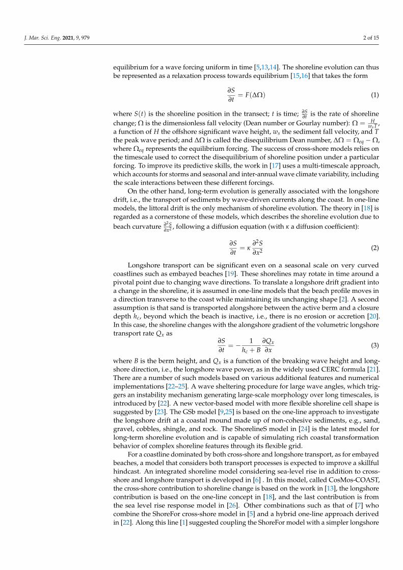
The 6 h interval ERA-Interim offshore wave data from the European Center for Medium-Range Weather Forecasts (ECMWF) from May 2013 to December 2015 are propagated andtransformed by the Simulating WAves Nearshore model (SWAN) up to 10 m water depthand at breaking point [34]. SWAN is a third-generation wave model for obtaining realisticestimates of wave parameters in coastal areas, lakes, and estuaries from given wind, bottom,and current conditions [35]. The bathymetry data input in SWAN is a combination of data ofthe General Bathymetric Chart of the Oceans (GEBCO) and COASTVAR measured topographydata (Figure 5). The resolution of GEBCO data is approximately 800 m. The COASTVARmeasured topography data are very detailed in the near-shore zone. The wave data results at10 m depth and at breaking point are used for shoreline evolution modeling. The time intervalof the wave fields including Hs, Tp, and α is 1 h. Locations of the point at 10 m depth and ofbreaker line used for extracting SWAN wave outputs are shown in Figure 6a. They are nearto the COASTVAR shoreline detection location. The breaking wave is defined indirectly fromthe significant wave height and the water depth extracted from SWAN outputs to calculatethe breaking index γ [7,36]. γ is the ratio of the wave height to the water depth. The criterionfor wave breaking is taken when γ is about 0.78. The SWAN computational grid of 20 m istoo large to define the locations where γ is 0.78. A region of 400 m× 400 m near the beachincluding the surf zone is thus extracted from the computational grid to find the grid cellshaving γ in the range from 0.4 to 0.8 [34]. Figure 6a,b shows the region of 400 m × 400 mextracted for the breaker line determination. It is clear that the range from 0.4 to 0.8 of thebreaking index provides the breaker line which is continuous along the shoreline and parallelto the shoreline (Figure 6a). The significant wave height and the wave direction at breakingpoint are calculated by taking mean value at these grid points. Figure 6c,d shows the waveroses at 10 m water depth and at breaking point, respectively. Figure 7a shows the time seriesof the significant wave height Hs at 10 m depth. It ranges from 0.01 m to 1.71 m and the meanvalue is 0.43 m. It is noticed that the significant wave height in summer has very small valuescorresponding with the large values of the surf similarity parameter (Figure 7b). The surfsimilarity parameter [37] or the Iribarren number ξ is used to classify breaker types, given by

ξ =m√

H∞/L∞(7)

where m is the beach slope, H∞ is the deep-water wave height, and L∞ is the deep-waterwave length. The surf similarity parameter ξ represents the influence of the beach slopeon the wave geometry. There are three main types of breaking, such as spilling (ξ < 0.5),plunging (0.5 < ξ < 3.3), and surging (ξ > 3.3) [38]. Figure 7b shows the time series of thesurf similarity parameter ξ. In this case, the wave parameters at 10 m depth were used tocalculate ξ.

J. Mar. Sci. Eng. 2021, 9, 979 7 of 15

GEBCO data grid points

Cai river estuary

800m

COASTVAR data points

Figure 5. Bathymetry data input includes GEBCO data grid points and COASTVAR measuredtopography data points.

(a)

5 10

15

Legend: Point at 10m depth

Breaker line

N

W

S

E

m

m

m

Tp (s)

N

W

S

E

m

m

m

Tp (s)

γ

(b)

(c) (d)

Figure 6. (a) Locations of point at 10 m depth and of breaker line used for extracting SWAN wavecharacteristics. (b) Breaker line along the shoreline at PF1 detected from a SWAN grid region of400 m × 400 m; colorbar indicates the breaking index. “x grid” is the index of “X”, while “y grid”is the index of “Y”; “pixel” is a grid cell of 20 m × 20 m. Directional plot of the significant waveheight Hs (circles) and the peak wave period Tp (colorbar) from SWAN at 10 m water depth (c) andat breaking point (d). The red line is the beach orientation. North (N) corresponds to 0.

J. Mar. Sci. Eng. 2021, 9, 979 8 of 15

(a)

0.0

0.5

1.0

1.5

2014 2015 2016

Hs (

m)

(b)

2

4

6

2014 2015 2016

Years

ξ

Figure 7. (a) Time series of SWAN significant wave height Hs at 10 m depth (green line) and the horizontal line at its meanvalue = 0.43 m (red dashed line). (b) Time series of the surf similarity parameter ξ (yellow line) and the horizontal line atthe threshold value of ξ = 3.3 (red dashed line).

4.3. Result

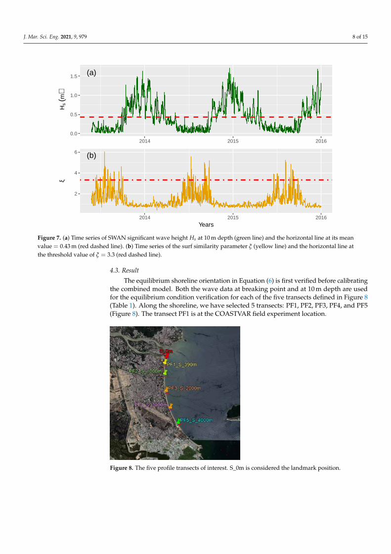
The equilibrium shoreline orientation in Equation (6) is first verified before calibratingthe combined model. Both the wave data at breaking point and at 10 m depth are usedfor the equilibrium condition verification for each of the five transects defined in Figure 8(Table 1). Along the shoreline, we have selected 5 transects: PF1, PF2, PF3, PF4, and PF5(Figure 8). The transect PF1 is at the COASTVAR field experiment location.

Figure 8. The five profile transects of interest. S_0m is considered the landmark position.

J. Mar. Sci. Eng. 2021, 9, 979 9 of 15

Table 1. Values of ψb, ψ10, αb, α10, βb, β10, and βm. βm is the beach orientation measured on GoogleEarth images.

Transect ψb ψ10 αb α10 βb β10 βm

PF1 −0.27 −58.53 2.68 18.02 2.54 −11.25 2

PF2 −0.53 −56.88 −5.12 12.87 −5.38 −15.57 −1

PF3 −0.99 −59.06 −13.58 4.60 −14.08 −24.93 −10

PF4 −1.38 −60.02 −25.77 −4.99 −26.46 −35 −22

PF5 −4.58 −70.16 −39.38 −14.87 −41.67 −49.95 −36

βm is the average of the beach orientation measured in time on Google Earth imagesduring the calibration period. Table 1 shows that βb is a closer guess to βm than β10which gives confidence in the SWAN simulations. The results indicate that ψb has a smallcontribution to the beach orientation. The assumption on the angles used in Equation (6)is thus validated. The wave data at breaking point will thus be used for the longshorecomponent of the combined model. The cross-shore component of the combined model (4)is calibrated with the SWAN wave data at 10 m depth (Figure 9a).

Nari

Haiyan

Figure 9. The combined model calibrated with DS1. (a) Time series of Ω (green line), Ωeq (redline), upper envelope (blue line) and lower envelope (brown line), vertical lines indicate the time ofNari and Haiyan typhoons. (b) Time series of measured shoreline position (red points); shorelineposition from combined model (black line); shoreline position from ShoreFor model (gray line).(c) Cross-shore contribution (purple line) and longshore contribution (green line).

J. Mar. Sci. Eng. 2021, 9, 979 10 of 15

The combined model calibrated with DS1 gives the smallest RMSE of 1.12 m forφ = 20 days (Figure 9b). The parameters a, b, c, and r are 0.0251, 4.9432, 0.0146, and 0.4702,respectively. The optimal value of φ = 20 days for the combined model is small in com-parison with 70 days found with the ShoreFor model alone. It indicates that the longshorecomponent interacts with the cross-shore equilibrium state. With the longshore contri-bution, the equilibrium Dean numbers are computed with a smaller memory decay φ,i.e., the modeled beach state reaches equilibrium on shorter time scales. Figure 9c showsa clear seasonal shoreline change of the longshore contribution at the Nha Trang beach.From November to January in winter monsoons, it has an eroding trend with an amplitudeof 5 m, and from February to May in summer monsoons, it has an accreting trend with anamplitude of 3.5 m. In the middle of October 2013 and early November 2013, the longshorecontribution gives a small accretion trend even though Nari and Haiyan typhoons hit thecoast (Figure 9c). The measured shoreline position indicates that these two typhoons havedriven strong erosion events, and then the beach has had a fast recovery immediately afterthat [29,31]. In fact, during the COASTVAR campaign, it was observed that a storm eventhit the coast and caused erosion but then the beach also quickly recovered [32,33,39,40]. Itappears that the longshore contribution of the model tends to favor accretion/recoveryimmediately after the storm (Figure 9c).

The combined model is also calibrated with DS2 which is longer than DS1 (Figure 10).This time, the smallest RMSE is 3.27 m for φ = 70 days. The three calibration-freeparameters—a, b, and c—are 0.0081, 1.1548, and 0.0113, respectively. The erosion ra-tio r is 0.2358. From Figure 10a, the upper and lower envelopes of Ω clearly show yearlycycles. Waves in Nha Trang are strongly affected by the tropical climate with two distinctseasons: small waves with small Ω in summer and strong waves with strong Ω in winter.Ωeq has a variability time scale of one year just as the forcing Ω. Figure 10a also shows howφ affects the equilibrium Dean number Ωeq computations. In the first part of winter, as theenvelope increases, the equilibrium Dean number Ωeq is less than the instantaneous Deannumber Ω, so the model gives a strong erosion (Figure 10b). Because φ = 70 days, Ωeq isaffected by the small values of Ω from the summer period. This φ value thus producesa strong phase shift of Ωeq. In the next phase, as Ωeq becomes larger than Ω, the modelgives an accretion (Figure 10b). Figure 10b shows that the modeled shoreline positionreproduces the observed annual cycle of erosion and accretion, although there are largediscrepancies during the accretion phase. Figure 10c shows that only a small part of theseasonal shoreline change is described by the longshore contribution while the synoptic toseasonal time scales of shoreline change are mainly due to the cross-shore contribution.

4.4. Discussion

The most striking result of the model is that the accretion sequence is poorly repro-duced during the summer monsoons (Figure 10b). This is due to the memory decay usedin the weighted averaging for Ωeq in Equation (5). During summer monsoons, the smallwave forcing leads to a small Ωeq, very similar to the instantaneous Dean number Ω, sothat the disequilibrium Dean number is small and induces a small shoreline variation. Thissuggests that an intra-seasonal memory decay is not appropriate for summer conditionsand a multi-scale approach should be considered [17,41]. Alternatively, here, the definitionof Ωeq is re-valuated for summer.

During much of summer monsoons, the surf similarity parameter ξ is higher than 3.3(Figure 7b). The breaking waves can be thus classified as surging breakers, and nearshorewaves may not even break at all. The shoreline measurements indicate that there are nobreaking waves, so the longshore contribution is zero, but small waves on a long periodstill contribute to cross-shore accretion. The surging breakers induce strong swash andgentle backwash that produces shoreward sand transport [42]. As a result, the shorelinetends to accrete in summer.

J. Mar. Sci. Eng. 2021, 9, 979 11 of 15

(a)

0

1

2

3

2014 2015 2016

Ω

(b)−10

0

10

2014 2015 2016

S (

m)

(c)−10

0

10

2014 2015 2016

Years

S (

m)

Figure 10. The combined model calibrated with DS2. (a) Time series of Ω (green line), Ωeq (red line), upper envelope (blueline), lower envelope (brown line) and inter-annual average (black line), (b) Time series of measured shoreline position(red points) and shoreline position from combined model (black line), (c) Cross-shore contribution (purple line), longshorecontribution (green line).

In the original ShoreFor formulation [14], the equilibrium forcing Ωeq was constant andrepresented an annual value. This formulation was more favorable to seasonal variations.In our case, Ω would be lower than Ωeq at the peak of summer and accretion wouldcontinue until the onset of winter monsoon. However, for Ωeq varying at intra-seasonalscale (to deal with winter monsoon pulses), the model looses its relaxation mechanism atthe annual scale, which is associated with swash processes and summer accretion.

To remedy to this summer limitation, we consider the special case of very low energywaves with surf similarity parameter ξ higher than 3.3. In this case, Ωeq is assigned a con-stant value of 0.8 (near the annual mean), so that the beach would accrete in summer whenΩ(t) < 0.8 and ξ > 3.3 (Figure 11a). Figure 11b confirms that the shoreline position fromthe combined model with modified Ωeq improves significantly and the modeled shorelineposition is now remarkably close to observations during the summer (compare Figure 11bwith Figure 10b). The RMSE is 2.25 m, which is much lower than the previous one (3.27 m).The values of the calibration parameters a, b, and c are 0.0239, 3.015, and 0.0195, respectively.The erosion ratio r is 0.5413, and the optimal memory decay φ is now 20 days instead of70 days in the previous case. The relatively short time scale of 20 days encompasses thatof winter monsoon pulses [28], on which the model can now focus more optimally. Thisis in line with the multi-scale approach of ShoreFor developed in [17,41], but within asimpler formulation. Figure 11c also shows that the seasonal fluctuation of the longshore

J. Mar. Sci. Eng. 2021, 9, 979 12 of 15

contribution is now more pronounced than in the previous calibration (Figure 10c). For alonger interannual evolution, a period of three years is still too short and we will rely inthe future on satellite monitoring for periods up to 30 years [43–45]. This will likely help inunderstanding the interaction between wave forcing and shoreline evolution at differenttime scales.

(a)

0

1

2

3

2014 2015 2016

Ω

(b)−10

0

10

2014 2015 2016

S (

m)

(c)−10

0

10

2014 2015 2016

Years

S (

m)

Figure 11. The combined model calibrated with DS2 and modified equilibrium Dean number in summer. (a) Time series ofΩ (light-blue line), Ωeq (red line), upper envelope (blue line), lower envelope (brown line). (b) Time series of measuredshoreline position (red points) and modeled shoreline position (black line). (c) Time series of the longshore contribution(green line) and the cross-shore contribution (purple line).

5. Conclusions

The results from the combined model calibrated with Nha Trang shoreline data andSWAN wave fields are an improvement over those of the ShoreFor model. The longshorecontribution slightly improves the variability of the modeled shoreline position, especiallywith the shoreline data DS1. Interestingly, the seasonal cycle of the coastline is weaklyaffected by the longshore contribution and is better explained by the cross-shore transport.

In addition, we suggest that the definition of the equilibrium Dean number shouldbe modified for very low-energy waves (ξ > 3.3), in summer, under conditions withoutintra-seasonal wave events. It is a way to resolve contrasting behaviors at multiple scales.Without this modification, it is difficult to find an optimal memory parameter φ thatrepresents in the same time the action of high-energy winter monsoon events at scales of3–20 days and annual recovery mechanisms associated with swash transport. By assigningan annual mean value to the equilibrium Dean number Ωeq when the surf similarity ξ0 ishigher than 3.3, we obtain a much smaller error of shoreline position. This enhancementsimply mimics the slow but long process of shoreline accretion under very light waves.

J. Mar. Sci. Eng. 2021, 9, 979 13 of 15

Although the combined model provides better predictive capabilities than the cross-shore model alone, the latter remains the main source of uncertainty at small time scales(<decades). A large part of the uncertainty appears related to the way Ωeq is defined. Ourresults clearly points to the relevance of a multi-scale approach in this regard, although ourmodified formulation keeps the advantage of simplicity.

Author Contributions: Conceptualization, E.B.; methodology: E.B., T.N., D.T.H.; software, Y.H.T.;validation, E.B., P.M., R.A. and Y.H.T.; data curation, R.A., D.H.T. and Y.H.T.; writing—original draftpreparation, Y.H.T.; writing—review and editing, E.B., P.M., R.A. and Y.H.T.; visualization, Y.H.T.;funding acquisition, D.T.H. and T.N. All authors have read and agreed to the published version ofthe manuscript.

Funding: This research is funded by Ho Chi Minh City University of Technology (HCMUT), VNU-HCM under grant number Tc-KTXD-2020-01.

Institutional Review Board Statement: Not applicable.

Informed Consent Statement: Not applicable.

Data Availability Statement: The data that support the findings of this study are available from thecorresponding author, [R.A. and D.H.T.], upon reasonable request.

Acknowledgments: This research has been conducted under the framework of CARE-Rescif initiativeand the Ho Chi Minh City University of Technology (HCMUT), VNU-HCM under grant numberTc-KTXD-2020-01. We acknowledge the support of time and facilities from HCMUT, VNU-HCM,LEGI-INPG, CARE-Rescif for this study. Y.H.T. was funded by the French Embassy in Hanoi for thePhD grant “Bourse d’Excellence”.

Conflicts of Interest: The authors declare no conflict of interest.

AbbreviationsThe following abbreviations are used in this manuscript:

COASTVAR Coastal Variability in West Africa and VietnamCosMos-COAST Coastal One-line Assimilated Simulation ToolECMWF European Center for Medium-Range Weather ForecastsGEBCO General Bathymetric Chart of the OceansRMSE root mean square errorSWAN Simulating WAves Nearshore model

References1. Tran, Y.H.; Barthélemy, E. Combined longshore and cross-shore shoreline model for closed embayed beaches. Coast. Eng. 2020,

158, 103692. [CrossRef]2. Hanson, H.; Kraus, N.C. GENESIS: Generalized Model for Simulating Shoreline Change. Report 1. Technical Reference; Coastal

Engineering Research Center: Vicksburg, MS, USA, 1989.3. Davidson, M.A.; Turner, I.L. A behavioral template beach profile model for predicting seasonal to interannual shoreline evolution.

J. Geophys. Res. Earth Surf. 2009, 114. [CrossRef]4. Castelle, B.; Marieu, V.; Bujan, S.; Ferreira, S.; Parisot, J.; Capo, S.; Sénéchal, N.; Chouzenoux, T. Equilibrium shoreline modelling

of a high-energy mesomacrotidal multiple-barred beach. Mar. Geol. 2014, 347, 85–94. [CrossRef]5. Splinter, K.D.; Turner, I.L.; Davidson, M.A.; Barnard, P.; Castelle, B.; Oltman-Shay, J. A generalized equilibrium model for

predicting daily to interannual shoreline response. J. Geophys. Res. Earth Surf. 2014, 119, 1936–1958. [CrossRef]6. Vitousek, S.; Barnard, P.L.; Limber, P.; Erikson, L.; Cole, B. A model integrating longshore and cross-shore processes for predicting

long-term shoreline response to climate change. J. Geophys. Res. Earth Surf. 2017, 122, 782–806. [CrossRef]7. Robinet, A.; Idier, D.; Castelle, B.; Marieu, V. On a reduced-complexity shoreline change model combining longshore and

cross-shore processes: The LX-Shore model. Environ. Model. Softw. 2018, 109, 1–16. [CrossRef]8. Montaño, J.; Coco, G.; Antolínez, J.A.; Beuzen, T.; Bryan, K.R.; Cagigal, L.; Castelle, B.; Davidson, M.A.; Goldstein, E.B.; Vos,

K.; et al. Blind testing of shoreline evolution models. Sci. Rep. 2020, 10, 2137. [CrossRef] [PubMed]9. Tomasicchio, G.R.; Francone, A.; Simmonds, D.J.; D’Alessandro, F.; Frega, F. Prediction of Shoreline Evolution. Reliability of a

General Model for the Mixed Beach Case. J. Mar. Sci. Eng. 2020, 8, 361. [CrossRef]10. Roelvink, J.A.; Van Banning, G.K.F.M. Design and development of delft3d and application to coastal morphodynamics. Oceanogr.

Lit. Rev. 1995, 11, 925.

J. Mar. Sci. Eng. 2021, 9, 979 14 of 15

11. Roelvink, D.; Reniers, A.J.H.M.; Van Dongeren, A.; Van Thiel de Vries, J.; Lescinski, J.; McCall, R. Xbeach model description andmanual. Unesco-Ihe Inst. Water Educ. Deltares Delft Univ. Technol. Rep. June 2010, 21, 2010.

12. Warren, I.R.; Bach, H.K. Mike 21: A modelling system for estuaries, coastal waters and seas. Environ. Softw. 1992, 7, 229–240.[CrossRef]

13. Yates, M.L.; Guza, R.T.; O’reilly, W.C. Equilibrium shoreline response: Observations and modeling. J. Geophys. Res. Ocean.2009, 114. [CrossRef]

14. Davidson, M.A.; Splinter, K.D.; Turner, I.L. A simple equilibrium model for predicting shoreline change. Coast. Eng. 2013,73, 191–202. [CrossRef]

15. Kriebel, D.L.; Dean, R.G. Convolution method for time-dependent beach-profile response. J. Waterw. Port Coast. Ocean. Eng. 1993,119, 204–226. [CrossRef]

16. Wright, L.D.; Short, A.D. Morphodynamic variability of surf zones and beaches: A synthesis. Mar. Geol. 1984, 56, 93–118.[CrossRef]

17. Schepper, R.; Almar, R.; Bergsma, E.; de Vries, S.; Reniers, A.; Davidson, M.; Splinter, K. Modelling Cross-Shore Shoreline Changeon Multiple Timescales and Their Interactions. J. Mar. Sci. Eng. 2021, 9, 582. [CrossRef]

18. Pelnard-Considère R. Theoretical Tests on the Shoreline Evolution of Sand and Gravel Beaches. In Proceedings of the 4èmesJournées de l’Hydraulique, Paris, France, 13–15 June 1956; pp. 289–298.

19. Turki, I.; Medina, R.; Coco, G.; Gonzalez, M. An equilibrium model to predict shoreline rotation of pocket beaches. Mar. Geol.2013, 346, 220–232. [CrossRef]

20. Dronkers, J. Dynamics of Coastal Systems; World Scientific: Singapore, 2005; Volume 25.21. Coastal Engineering Research Center (US). Shore Protection Manual; Department of the Army, Waterways Experiment Station,

Corps of Engineers, Coastal Engineering Research Center: Washington, DC, USA, 1984.22. Ashton, A.; Murray, A.B.; Arnoult, O. Formation of coastline features by large-scale instabilities induced by high-angle waves.

Nature 2001, 414, 296–300. [CrossRef]23. Hurst, M.D.; Barkwith, A.; Ellis, M.A.; Thomas, C.W.; Murray, A.B. Exploring the sensitivities of crenulate bay shorelines to wave

climates using a new vector-based one-line model. J. Geophys. Res. Earth Surf. 2015, 120, 2586–2608. [CrossRef]24. Roelvink, D.; Huisman, B.; Elghandour, A.; Ghonim, M.; Reyns, J. Efficient modelling of complex sandy coastal evolution at

monthly to century time scales. Front. Mar. Sci. 2020, 7, 535. [CrossRef]25. Medellin, G.; Torres-Freyermuth, A.; Tomasicchio, G.R.; Francone, A.; Tereszkiewicz, P.A.; Lusito, L.; Palemon-Arcos, L.; Lopez,

J. Field and Numerical Study of Resistance and Resilience on a Sea Breeze Dominated Beach in Yucatan (Mexico). Water 2018,10, 1806. [CrossRef]

26. Bruun, P. Sea-level rise as a cause of shore erosion. J. Waterw. Harb. Div. 1962, 88, 117–130. [CrossRef]27. Thuan, D.H.; Almar, R.; Marchesiello, P.; Viet, N.T. Video Sensing of Nearshore Bathymetry Evolution with Error Estimate. J. Mar.

Sci. Eng. 2019, 7, 233. [CrossRef]28. Marchesiello, P.; Kestenare, E.; Almar, R.; Boucharel, J.; Nguyen, N.M. Longshore drift produced by climate-modulated monsoons

and typhoons in the South China Sea. J. Mar. Syst. 2020, 211, 103399. [CrossRef]29. Almar, R.; Marchesiello, P.; Almeida, L.P.; Thuan, D.H.; Tanaka, H.; Viet, N.T. Shoreline response to a sequence of typhoon and

monsoon events. Water 2017, 9, 364. [CrossRef]30. Bertsimas, D.; Tsitsiklis, J. Simulated annealing. Stat. Sci. 1993, 8, 10–15 [CrossRef]31. Thuan, D.H.; Binh, L.T.; Viet, N.T.; Hanh, D.K.; Almar, R.; Marchesiello, P. Typhoon impact and recovery from continuous video

monitoring: A case study from Nha Trang Beach, Vietnam. J. Coast. Res. 2016, 75, 263–267. [CrossRef]32. Almeida, L.P.; Almar, R.; Blenkinsopp, C.; Senechal, N.; Bergsma, E.; Floc’h, F.; Caulet, C.; Biausque, M.; Marchesiello, P.;

Grandjean, P.; et al. Lidar Observations of the Swash Zone of a Low-Tide Terraced Tropical Beach under Variable WaveConditions: The Nha Trang (Vietnam) COASTVAR Experiment. J. Mar. Sci. Eng. 2020, 8, 302. [CrossRef]

33. Andriolo, U.; Almeida, L.P.; Almar, R. Coupling terrestrial LiDAR and video imagery to perform 3D intertidal beach topography.Coast. Eng. 2018, 140, 232–239. [CrossRef]

34. Tran, H.Y. Modeling Long Term Shoreline Evolution and Coastal Erosion. Ph.D. Thesis, Université Grenoble Alpes, Grenoble,France, 2018.

35. Booij, N.R.R.C.; Ris, R.C.; Holthuijsen, L.H. A third-generation wave model for coastal regions: 1. Model description andvalidation. J. Geophys. Res. Ocean. 1999, 104, 7649–7666. [CrossRef]

36. Bertin, X.; Castelle, B.; Chaumillon, E.; Butel, R.; Quique, R. Longshore transport estimation and inter-annual variability at ahigh-energy dissipative beach: St. Trojan beach, SW Oléron Island, France. Cont. Shelf Res. 2008, 28, 1316–1332. [CrossRef]

37. Battjes, J.A. Surf similarity. In Proceedings of the 14th International Conference on Coastal Engineering, Copenhagen, Denmark,24–28 June 1975; pp. 466–480.

38. Galvin, C.J., Jr. Breaker type classification on three laboratory beaches. J. Geophys. Res. 1968, 73, 3651–3659. [CrossRef]39. Daly, C.; Floc’h, F.; Almeida, L.P.; Almar, R. Modelling accretion at Nha Trang Beach, Vietnam. Icoastal Dyn. 2017, 170, 1886–1896.40. Dalya, C.J.; Floc’h, F.; Almeida, L.P.; Almara, R.; Jaud, M. Morphodynamic modelling of beach cusp formation: The role of wave

forcing and sediment composition. Geomorphology 2021, 389, 107798. [CrossRef]41. Davidson, M. Forecasting coastal evolution on time-scales of days to decades. Coast. Eng. 2021, 168, 103928. [CrossRef]42. Bird, E.C. Coastal Geomorphology: An Introduction; John Wiley & Sons: Hoboken, NJ, USA, 2011.

J. Mar. Sci. Eng. 2021, 9, 979 15 of 15

43. Vos, K.; Harley, M.D.; Splinter, K.D.; Walker, A.; Turner, I.L. Beach Slopes from Satellite-Derived Shorelines. Geophys. Res. Lett.2020, 47, e2020GL088365. [CrossRef]

44. Bergsma, E.W.; Almar, R. Coastal coverage of ESA’Sentinel 2 mission. Adv. Space Res. 2020, 65, 2636–2644. [CrossRef]45. Taveneau, A.; Almar, R.; Bergsma, E.W.; Sy, B.A.; Ndour, A.; Sadio, M.; Garlan, T. Observing and Predicting Coastal Erosion at the

Langue de Barbarie Sand Spit around Saint Louis (Senegal, West Africa) through Satellite-Derived Digital Elevation Model andShoreline. Remote Sens. 2021, 13, 2454. [CrossRef]