This content has been downloaded from IOPscience. Please scroll down to see the full text.

Download details:

IP Address: 193.137.92.44

This content was downloaded on 26/05/2017 at 17:37

Please note that terms and conditions apply.

Combined performance studies for electrons at the 2004 ATLAS combined test-beam

View the table of contents for this issue, or go to the journal homepage for more

2010 JINST 5 P11006

(http://iopscience.iop.org/1748-0221/5/11/P11006)

Home Search Collections Journals About Contact us My IOPscience

You may also be interested in:

Photon reconstruction in the ATLAS Inner Detector and Liquid Argon Barrel Calorimeter at the 2004

Combined Test Beam

E Abat, J M Abdallah, T N Addy et al.

A layer correlation technique for pion energy calibration at the 2004 ATLAS Combined Beam Test

E Abat, J M Abdallah, T N Addy et al.

ALICE: Physics Performance Report, Volume II

ALICE Collaboration, B Alessandro, F Antinori et al.

Operation and performance of the ATLAS semiconductor tracker

The ATLAS collaboration

Performance of the ATLAS Transition Radiation Tracker in Run 1 of the LHC: tracker properties

M. Aaboud, G. Aad, B. Abbott et al.

The Role of the LAr Calorimeter in the Search for H in ATLAS

G Unal and on behalf of the ATLAS Collaboration)

Monitoring and data quality assessment of the ATLAS liquid argon calorimeter

The ATLAS collaboration

Physics of cascading shower generation and propagation in matter: principles of high-energy,

ultrahigh-energy and compensating calorimetry

Claude Leroy and Pier-Giorgio Rancoita

Electromagnetic response of a highly granular hadronic calorimeter

The CALICE collaboration, C Adloff, J Blaha et al.

2010 JINST 5 P11006

PUBLISHED BY IOP PUBLISHING FOR SISSA

RECEIVED: September 6, 2010ACCEPTED: November 1, 2010

PUBLISHED: November 25, 2010

Combined performance studies for electrons at the2004 ATLAS combined test-beam

E. Abat, k,1 J.M. Abdallah, f T.N. Addy, ag P. Adragna, cc M. Aharrouche, ba

A. Ahmad, cm,2 T.P.A. Akesson, ay M. Aleksa, s C. Alexa, n K. Anderson, t

A. Andreazza, be,b f F. Anghinolfi, s A. Antonaki, e G. Arabidze, e E. Arik, k T. Atkinson, bd

J. Baines, c f O.K. Baker, dd D. Banfi, be,b f S. Baron, s A.J. Barr, bs R. Beccherle, a j

H.P. Beck, i B. Belhorma, aw P.J. Bell, bb,3 D. Benchekroun, q D.P. Benjamin, ac

K. Benslama, cg E. Bergeaas Kuutmann, cp,4 J. Bernabeu, cz H. Bertelsen, v S. Binet, bq

C. Biscarat, ad V. Boldea, n V.G. Bondarenko, bk M. Boonekamp, c j M. Bosman, f

C. Bourdarios, bq Z. Broklova, ca D. Burckhart Chromek, s V. Bychkov, an J. Callahan, ai

D. Calvet, u M. Canneri, bw M. Capeans Garrido, s M. Caprini, n L. Cardiel Sas, s T. Carli, s

L. Carminati, be,b f J. Carvalho, p,by M. Cascella, bw M.V. Castillo, cz A. Catinaccio, s

D. Cauz,ak D. Cavalli, be M. Cavalli Sforza, f V. Cavasinni, bw S.A. Cetin, k H. Chen, j

R. Cherkaoui, cd L. Chevalier, c j F. Chevallier, aw S. Chouridou, cx M. Ciobotaru, cv

M. Citterio, be A. Clark, ae B. Cleland, bx M. Cobal, ak E. Cogneras, i P. Conde Muino, by

M. Consonni, be,b f S. Constantinescu, n T. Cornelissen, s,5 S. Correard, w

A. Corso Radu, s G. Costa, be M.J. Costa, cz D. Costanzo, cl S. Cuneo, a j P. Cwetanski, ai

D. Da Silva, ch M. Dam,v M. Dameri, a j H.O. Danielsson, s D. Dannheim, s G. Darbo, a j

T. Davidek, ca K. De,d P.O. Defay,u B. Dekhissi, ax J. Del Peso, az T. Del Prete, bw

M. Delmastro, s F. Derue,av L. Di Ciaccio, ar B. Di Girolamo, s S. Dita,n F. Dittus, s

F. Djama,w T. Djobava, cs D. Dobos, aa,6 M. Dobson, s B.A. Dolgoshein, bk A. Dotti, bw

G. Drake,b Z. Drasal, ca N. Dressnandt, bu C. Driouchi, v J. Drohan, cw W.L. Ebenstein, ac

P. Eerola, ay,7 I. Efthymiopoulos, s K. Egorov, ai T.F. Eifert, s K. Einsweiler, h

M. El Kacimi, as M. Elsing, s D. Emelyanov, c f,8 C. Escobar, cz A.I. Etienvre, c j A. Fabich, s

1Deceased2Now at SUNY, Stony Brook, United States of America3Now at Universite de Geneve, Switzerland4Now at DESY, Zeuthen, Germany5Now at INFN Genova and Universita di Genova, Italy6Now at CERN7Now at University of Helsinki, Finland8Now at Joint Institute for Nuclear Research, Dubna, Russia

c© 2010 IOP Publishing Ltd and SISSA doi:10.1088/1748-0221/5/11/P11006

2010 JINST 5 P11006

K. Facius, v A.I. Fakhr-Edine, o M. Fanti, be,b f A. Farbin, d P. Farthouat, s

D. Fassouliotis, e L. Fayard, bq R. Febbraro, u O.L. Fedin, bv A. Fenyuk, cb

D. Fergusson, h P. Ferrari, s,9 R. Ferrari, bt B.C. Ferreira, ch A. Ferrer, cz D. Ferrere, ae

G. Filippini, u T. Flick, dc D. Fournier, bq P. Francavilla, bw D. Francis, s R. Froeschl, s,10

D. Froidevaux, s E. Fullana, b S. Gadomski, ae G. Gagliardi, a j P. Gagnon, ai M. Gallas, s

B.J. Gallop, c f S. Gameiro, s K.K. Gan, bp R. Garcia, az C. Garcia, cz I.L. Gavrilenko, b j

C. Gemme,a j P. Gerlach, dc N. Ghodbane, u V. Giakoumopoulou, e V. Giangiobbe, bw

N. Giokaris, e G. Glonti, an T. Goettfert, bm T. Golling, h,11 N. Gollub, s A. Gomes, at,au,by

M.D. Gomez,ae S. Gonzalez-Sevilla, cz,12 M.J. Goodrick, r G. Gorfine, bo B. Gorini, s

D. Goujdami, o K-J. Grahn, aq P. Grenier, u,13 N. Grigalashvili, an Y. Grishkevich, bl

J. Grosse-Knetter, l ,14 M. Gruwe, s C. Guicheney, u A. Gupta, t C. Haeberli, i

R. Haertel, bm,15 Z. Hajduk, y H. Hakobyan, de M. Hance,bu J.D. Hansen, v P.H. Hansen, v

K. Hara,cu A. Harvey Jr., ag R.J. Hawkings, s F.E.W. Heinemann, bs

A. Henriques Correia, s T. Henss, dc L. Hervas, s E. Higon, cz J.C. Hill, r J. Hoffman, z

J.Y. Hostachy, aw I. Hruska, ca F. Hubaut, w F. Huegging, l W. Hulsbergen, s,16

M. Hurwitz, t L. Iconomidou-Fayard, bq E. Jansen, ce I. Jen-La Plante, t

P.D.C. Johansson, cl K. Jon-And, cp M. Joos, s S. Jorgensen, f J. Joseph, h

A. Kaczmarska, y,17 M. Kado, bq A. Karyukhin, cb M. Kataoka, s,18 F. Kayumov, b j

A. Kazarov, bv P.T. Keener, bu G.D. Kekelidze, an N. Kerschen, cl S. Kersten, dc

A. Khomich, bc G. Khoriauli, an E. Khramov, an A. Khristachev, bv J. Khubua, an

T.H. Kittelmann, v,19 R. Klingenberg, aa E.B. Klinkby, ac P. Kodys, ca T. Koffas, s

S. Kolos, cv S.P. Konovalov, b j N. Konstantinidis, cw S. Kopikov, cb I. Korolkov, f

V. Kostyukhin, a j,20 S. Kovalenko, bv T.Z. Kowalski, x K. Kruger, s,21 V. Kramarenko, bl

L.G. Kudin, bv Y. Kulchitsky, bi C. Lacasta, cz R. Lafaye, ar B. Laforge, av W. Lampl, c

F. Lanni, j S. Laplace, ar T. Lari, be A-C. Le Bihan, s,22 M. Lechowski, bq

F. Ledroit-Guillon, aw G. Lehmann, s R. Leitner, ca D. Lelas, bq C.G. Lester, r Z. Liang, z

P. Lichard, s W. Liebig, bo A. Lipniacka, g M. Lokajicek, bz L. Louchard, u K.F. Lourerio, bp

A. Lucotte, aw F. Luehring, ai B. Lund-Jensen, aq B. Lundberg, ay H. Ma, j

9Now at Nikhef National Institute for Subatomic Physics, Amsterdam, Netherlands10Corresponding author,robert.froeschl@cern.ch11Now at Yale University, New Haven, U.S.A.12Now at Universite de Geneve, Switzerland13Now at SLAC, Stanford, U.S.A.14Now at Georg-August-Universitaet, Goettingen, Germany15Now at Versicherungskammer Bayern, Munich, Germany16Now at Nikhef National Institute for Subatomic Physics, Amsterdam, Netherlands17Now at Universite Pierre et Marie Curie (Paris 6) and Universite Denis Diderot (Paris-7), France18Now at Laboratoire de Physique de Particules (LAPP), Annecy-le-Vieux, France19Now at University of Pittsburgh, U.S.A.20Now at Physikalisches Institut der Universitaet Bonn, Germany21Now at Universitat Heidelberg, Germany22Now at IPHC, Universit’e de Strasbourg, CNRS/IN2P3, Strasbourg, France

2010 JINST 5 P11006

R. Mackeprang, v A. Maio, at,au,by V.P. Maleev,bv F. Malek,aw L. Mandelli, be J. Maneira, by

M. Mangin-Brinet, ae,23 A. Manousakis, e L. Mapelli, s C. Marques, by S.Marti i Garcia, cz

F. Martin, bu M. Mathes, l M. Mazzanti, be K.W. McFarlane, ag R. McPherson, da

G. Mchedlidze, cs S. Mehlhase, ah C. Meirosu, s Z. Meng,ck C. Meroni, be V. Mialkovski, an

B. Mikulec, ae,24 D. Milstead, cp I. Minashvili, an B. Mindur, x V.A. Mitsou, cz S. Moed,ae,25

E. Monnier, w G. Moorhead, bd P. Morettini, a j S.V. Morozov, bk M. Mosidze, cs

S.V. Mouraviev, b j E.W.J. Moyse, s A. Munar, bu A. Myagkov, cb A.V. Nadtochi, bv

K. Nakamura, cu,26 P. Nechaeva, a j,27 A. Negri, bt S. Nemecek, bz M. Nessi, s

S.Y. Nesterov, bv F.M. Newcomer, bu I. Nikitine, cb K. Nikolaev, an I. Nikolic-Audit, av

H. Ogren, ai S.H. Oh,ac S.B. Oleshko, bv J. Olszowska, y A. Onofre, bg,by

C. Padilla Aranda, s S. Paganis, cl D. Pallin, u D. Pantea,n V. Paolone, bx F. Parodi, a j

J. Parsons, bn S. Parzhitskiy, an E. Pasqualucci, ci S.M. Passmored, s J. Pater, bb

S. Patrichev, bv M. Peez,az V. Perez Reale,bn L. Perini, be,b f V.D. Peshekhonov, an

J. Petersen, s T.C. Petersen, v R. Petti, j,28 P.W. Phillips, c f J. Pina, at,au,by B. Pinto, by

F. Podlyski, u L. Poggioli, bq A. Poppleton, s J. Poveda, db P. Pralavorio, w L. Pribyl, s

M.J. Price, s D. Prieur, c f C. Puigdengoles, f P. Puzo,bq O. Røhne,br F. Ragusa, be,b f

S. Rajagopalan, j K. Reeves, dc,29 I. Reisinger, aa C. Rembser, s

P.A. Bruckman de Renstrom, bs P. Reznicek, ca M. Ridel, av P. Risso, a j I. Riu,ae,30

D. Robinson, r C. Roda,bw S. Roe,s O. Rohne, br A. Romaniouk, bk D. Rousseau, bq

A. Rozanov, w A. Ruiz, cz N. Rusakovich, an D. Rust, ai Y.F. Ryabov, bv V. Ryjov, s

O. Salto, f B. Salvachua, b A. Salzburger, al,31 H. Sandaker, g C. Santamarina Rios, s

L. Santi, ak C. Santoni, u J.G. Saraiva, at,au,by F. Sarri, bw G. Sauvage, ar L.P. Says, u

M. Schaefer, aw V.A. Schegelsky, bv C. Schiavi, a j J. Schieck, bm G. Schlager, s

J. Schlereth, b C. Schmitt, ba J. Schultes, dc P. Schwemling, av J. Schwindling, c j

J.M. Seixas, ch D.M. Seliverstov, bv L. Serin, bq A. Sfyrla, ae,32 N. Shalanda, bh C. Shaw,a f

T. Shin, ag A. Shmeleva, b j J. Silva, by S. Simion, bq M. Simonyan, ar J.E. Sloper, s

S.Yu. Smirnov, bk L. Smirnova, bl C. Solans, cz A. Solodkov, cb O. Solovianov, cb

I. Soloviev, bv V.V. Sosnovtsev, bk F. Spano,bn P. Speckmayer, s S. Stancu, cv R. Stanek, b

E. Starchenko, cb A. Straessner, ab S.I. Suchkov, bk M. Suk,ca R. Szczygiel, x

F. Tarrade, j F. Tartarelli, be P. Tas,ca Y. Tayalati, u F. Tegenfeldt, am R. Teuscher, ct

M. Thioye, cq V.O. Tikhomirov, b j C.J.W.P. Timmermans, ce S. Tisserant, w B. Toczek, x

23Now at Laboratoire de Physique Subatomique et de CosmologieCNRS/IN2P3, Grenoble, France24Now at CERN25Now at Harvard University, Cambridge, U.S.A.26Now at ICEPP, Tokyo, Japan27Now at P.N. Lebedev Institute of Physics, Moscow, Russia28Now at University of South Carolina, Columbia, U.S.A.29Now at UT Dallas30Now at IFAE, Barcelona, Spain31Now at CERN32Now at CERN

2010 JINST 5 P11006

L. Tremblet, s C. Troncon, be P. Tsiareshka, bi M. Tyndel, c f M.Karagoez. Unel, bs

G. Unal,s G. Unel,ai G. Usai, t R. Van Berg, bu A. Valero, cz S. Valkar, ca J.A. Valls, cz

W. Vandelli, s F. Vannucci, av A. Vartapetian, d V.I. Vassilakopoulos, ag L. Vasilyeva, b j

F. Vazeille, u F. Vernocchi, a j Y. Vetter-Cole, z I. Vichou, cy V. Vinogradov, an J. Virzi, h

I. Vivarelli, bw J.B.de. Vivie, w,33 M. Volpi, f T. Vu Anh, ae,34 C. Wang,ac M. Warren, cw

J. Weber, aa M. Weber,c f A.R. Weidberg, bs J. Weingarten, l ,35 P.S. Wells, s P. Werner, s

S. Wheeler, a M. Wiessmann, bm H. Wilkens, s H.H. Williams, bu I. Wingerter-Seez, ar

Y. Yasu,ap A. Zaitsev, cb A. Zenin, cb T. Zenis, m Z. Zenonos, bw H. Zhang, w A. Zhelezko bk

and N. Zhou bn

aUniversity of Alberta, Department of Physics, Centre for Particle Physics,Edmonton, AB T6G 2G7, Canada

bArgonne National Laboratory, High Energy Physics Division,9700 S. Cass Avenue, Argonne IL 60439, United States of America

cUniversity of Arizona, Department of Physics, Tucson, AZ 85721, United States of AmericadUniversity of Texas at Arlington, Department of Physics,Box 19059, Arlington, TX 76019, United States of America

eUniversity of Athens, Nuclear & Particle Physics Department of Physics, Panepistimiopouli Zografou, GR15771 Athens, Greece

f Institut de Fisica d’Altes Energies, IFAE, Universitat Autonoma de Barcelona, Edifici Cn, ES - 08193Bellaterra (Barcelona) Spain

gUniversity of Bergen, Department for Physics and Technology, Allegaten 55, NO - 5007 Bergen, NorwayhLawrence Berkeley National Laboratory and University of California, Physics Division, MS50B-6227, 1Cyclotron Road, Berkeley, CA 94720, United States of America

iUniversity of Bern, Laboratory for High Energy Physics, Sidlerstrasse 5, CH - 3012 Bern, SwitzerlandjBrookhaven National Laboratory, Physics Department, Bldg. 510A, Upton,NY 11973, United States of America

kBogazici University, Faculty of Sciences, Department of Physics, TR - 80815 Bebek-Istanbul, Turkeyl Physikalisches Institut der Universitaet Bonn, Nussallee12, D - 53115 Bonn, Germany

mComenius University, Faculty of Mathematics Physics & Informatics, Mlynska dolina F2, SK - 84248Bratislava, Slovak Republic

nNational Institute of Physics and Nuclear Engineering (Bucharest -IFIN-HH), P.O. Box MG-6, R-077125Bucharest, Romania

oUniversite Cadi Ayyad, Marrakech, MoroccopDepartment of Physics, University of Coimbra, P-3004-516 Coimbra, PortugalqUniversite Hassan II, Faculte des Sciences Ain Chock, B.P. 5366, MA - Casablanca, MoroccorCavendish Laboratory, University of Cambridge, J J ThomsonAvenue, Cambridge CB3 0HE, UnitedKingdom

sEuropean Laboratory for Particle Physics (CERN), CH-1211 Geneva 23, SwitzerlandtUniversity of Chicago, Enrico Fermi Institute,5640 S. Ellis Avenue, Chicago, IL 60637, United States of America

33Now at LAL-Orsay, France34Now at Universitat Mainz, Mainz, Germany35Now at Georg-August-Universitaet, Goettingen, Germany

2010 JINST 5 P11006

uLaboratoire de Physique Corpusculaire (LPC), IN2P3-CNRS,Universite Blaise-Pascal Clermont-Ferrand,FR - 63177 Aubiere, France

vNiels Bohr Institute, University of Copenhagen, Blegdamsvej 17, DK - 2100 Kobenhavn 0, DenmarkwUniversite Mediterranee, Centre de Physique des Particules de Marseille,CNRS/IN2P3, F-13288 Marseille, France

xFaculty of Physics and Applied Computer Science of the AGH-University of Science and Technology,(FPACS, AGH-UST), al. Mickiewicza 30, PL-30059 Cracow, Poland

yThe Henryk Niewodniczanski Institute of Nuclear Physics, Polish Academy of Sciences, ul. Radzikowskiego152, PL - 31342 Krakow Poland

zSouthern Methodist University, Physics Department, 106 Fondren Science Building, Dallas, TX 75275-0175, United States of America

aaUniversitaet Dortmund, Experimentelle Physik IV, DE - 44221 Dortmund, GermanyabTechnical University Dresden, Institut fuer Kern- und Teilchenphysik,

Zellescher Weg 19, D-01069 Dresden, GermanyacDuke University, Department of Physics Durham, NC 27708, United States of AmericaadCentre de Calcul CNRS/IN2P3, Lyon, FranceaeUniversite de Geneve, Section de Physique, 24 rue Ernest Ansermet, CH - 1211 Geneve 4, Switzerlanda f University of Glasgow, Department of Physics and Astronomy, UK - Glasgow G12 8QQ, United KingdomagHampton University, Department of Physics, Hampton, VA 23668, United States of AmericaahInstitute of Physics, Humboldt University, Berlin, Newtonstrasse 15, D-12489 Berlin, GermanyaiIndiana University, Department of Physics,

Swain Hall West 117, Bloomington, IN 47405-7105, United States of Americaa jINFN Genova and Universita di Genova, Dipartimento di Fisica,

via Dodecaneso 33, IT - 16146 Genova, ItalyakINFN Gruppo Collegato di Udine and Universita di Udine, Dipartimento di Fisica, via delle Scienze 208,

IT - 33100 Udine;INFN Gruppo Collegato di Udine and ICTP, Strada Costiera 11,IT - 34014 Trieste, Italy

alInstitut fuer Astro- und Teilchenphysik, Technikerstrasse 25, A - 6020 Innsbruck, AustriaamIowa State University, Department of Physics and Astronomy, Ames High Energy Physics Group, Ames,

IA 50011-3160, United States of AmericaanJoint Institute for Nuclear Research, JINR Dubna, RU - 141 980 Moscow Region, RussiaaoInstitut fuer Prozessdatenverarbeitung und Elektronik, Karlsruher Institut fuer Technologie, Campus Nord,

Hermann-v.Helmholtz-Platz 1, D-76344 Eggenstein-LeopoldshafenapKEK, High Energy Accelerator Research Organization,

1-1 Oho Tsukuba-shi, Ibaraki-ken 305-0801, JapanaqRoyal Institute of Technology (KTH), Physics Department, SE - 106 91 Stockholm, SwedenarLaboratoire de Physique de Particules (LAPP), Universite de Savoie, CNRS/IN2P3,

Annecy-le-Vieux Cedex, FranceasLaboratoire de Physique de Particules (LAPP), Universite de Savoie, CNRS/IN2P3, Annecy-le-Vieux

Cedex, France and Universite Cadi Ayyad, Marrakech, MoroccoatDepartamento de Fisica, Faculdade de Ciencias, Universidade de Lisboa, P-1749-016 Lisboa, PortugalauCentro de Fısica Nuclear da Universidade de Lisboa, P-1649-003 Lisboa, PortugalavUniversite Pierre et Marie Curie (Paris 6) and Universite Denis Diderot (Paris-7), Laboratoire de Physique

Nucleaire et de Hautes Energies, CNRS/IN2P3,Tour 33 4 place Jussieu, FR - 75252 Paris Cedex 05, France

2010 JINST 5 P11006

awLaboratoire de Physique Subatomique et de Cosmologie CNRS/IN2P3, Universite Joseph Fourier INPG,53 avenue des Martyrs, FR - 38026 Grenoble Cedex, France

axLaboratoire de Physique Theorique et de Physique des Particules, Universite Mohammed Premier,Oujda, Morocco

ayLunds universitet, Naturvetenskapliga fakulteten, Fysiska institutionen,Box 118, SE - 221 00, Lund, Sweden

azUniversidad Autonoma de Madrid, Facultad de Ciencias, Departamento de Fisica Teorica,ES - 28049 Madrid, Spain

baUniversitat Mainz, Institut fur Physik, Staudinger Weg 7, DE 55099, GermanybbSchool of Physics and Astronomy, University of Manchester,UK - Manchester M13 9PL, United KingdombcUniversitaet Mannheim, Lehrstuhl fuer Informatik V, B6, 23-29, DE - 68131 Mannheim, GermanybdSchool of Physics, University of Melbourne, AU - Parkvill, Victoria 3010, AustraliabeINFN Sezione di Milano, via Celoria 16, IT - 20133 Milano, Italyb f Universita di Milano, Dipartimento di Fisica, via Celoria 16, IT - 20133 Milano, ItalybgDepartamento de Fisica, Universidade do Minho, P-4710-057Braga, PortugalbhB.I. Stepanov Institute of Physics, National Academy of Sciences of Belarus, Independence Avenue 68,

Minsk 220072, Republic of BelarusbiB.I. Stepanov Institute of Physics, National Academy of Sciences of Belarus, Independence Avenue 68,

Minsk 220072, Republic of Belarus and Joint Institute for Nuclear Research, JINR Dubna, RU - 141 980Moscow Region, Russia

b jP.N. Lebedev Institute of Physics, Academy of Sciences, Leninsky pr. 53, RU - 117 924, Moscow, RussiabkMoscow Engineering & Physics Institute (MEPhI), Kashirskoe Shosse 31, RU - 115409 Moscow, RussiablLomonosov Moscow State University, Skobeltsyn Institute of Nuclear Physics, RU - 119 991 GSP-1

Moscow Lenskiegory 1-2, RussiabmMax-Planck-Institut fur Physik, (Werner-Heisenberg-Institut),

Fohringer Ring 6, 80805 Munchen, GermanybnColumbia University, Nevis Laboratory, 136 So. Broadway, Irvington, NY 10533, United States of AmericaboNikhef National Institute for Subatomic Physics, Kruislaan 409,

P.O. Box 41882, NL - 1009 DB Amsterdam, NetherlandsbpOhio State University, 191 West WoodruAve, Columbus, OH 43210-1117, United States of AmericabqLAL, Universite Paris-Sud, IN2P3/CNRS, Orsay, FrancebrUniversity of Oslo, Department of Physics, P.O. Box 1048, Blindern T, NO - 0316 Oslo, NorwaybsDepartment of Physics, Oxford University, Denys WilkinsonBuilding,

Keble Road, Oxford OX1 3RH, United KingdombtUniversita di Pavia, Dipartimento di Fisica Nucleare e Teorica and INFN Pavia,

Via Bassi 6 IT-27100 Pavia, ItalybuUniversity of Pennsylvania, Department of Physics, High Energy Physics, 209 S. 33rd Street Philadelphia,

PA 19104, United States of AmericabvPetersburg Nuclear Physics Institute, RU - 188 300 Gatchina, RussiabwUniversitadi Pisa, Dipartimento di Fisica E. Fermi and INFN Pisa,

Largo B.Pontecorvo 3, IT - 56127 Pisa, ItalybxUniversity of Pittsburgh, Department of Physics and Astronomy, 3941 O’Hara Street, Pittsburgh, PA

15260, United States of AmericabyLaboratorio de Instrumentacao e Fisica Experimental de Particulas - LIP, and SIM/Univ. de Lisboa,

Avenida Elias Garcia 14-1, PT - 1000-149, Lisboa, Portugal

2010 JINST 5 P11006

bzAcademy of Sciences of the Czech Republic, Institute of Physics and Institute for Computer Science, NaSlovance 2, CZ - 18221 Praha 8, Czech Republic

caCharles University in Prague, Faculty of Mathematics and Physics, Institute of Particle and NuclearPhysics, V Holesovickach 2, CZ - 18000 Praha 8, Czech Republic

cbInstitute for High Energy Physics (IHEP), Federal Agency ofAtom. Energy, Moscow Region, RU - 142284 Protvino, Russia

ccQueen Mary, University of London, Mile End Road, E1 4NS, London, United KingdomcdUniversite Mohammed V, Faculte des Sciences, BP 1014, MO - Rabat, MoroccoceRadboud University Nijmegen/NIKHEF, Dept. of Exp. High Energy Physics, Toernooiveld 1, NL - 6525

ED Nijmegen, Netherlandsc f Rutherford Appleton Laboratory, Science and Technology Facilities Council, Harwell Science and Inno-

vation Campus, Didcot OX11 0QX, United KingdomcgUniversity of Regina, Physics Department, CanadachUniversidade Federal do Rio De Janeiro, Instituto de Fisica, Caixa Postal 68528, Ilha do Fundao, BR -

21945-970 Rio de Janeiro, BrazilciUniversita La Sapienza, Dipartimento di Fisica and INFN Roma I,

Piazzale A. Moro 2, IT- 00185 Roma, Italyc jCommissariat a l’Enegie Atomique (CEA), DSM/DAPNIA, Centre d’Etudes de Saclay,

91191 Gif-sur-Yvette, FranceckInsitute of Physics, Academia Sinica, TW - Taipei 11529, Taiwan and Shandong University, School of

Physics, Jinan, Shandong 250100, P. R. ChinaclUniversity of Sheffield, Department of Physics & Astronomy,

Hounseld Road, Sheffield S3 7RH, United KingdomcmInsitute of Physics, Academia Sinica, TW - Taipei 11529, TaiwancnSLAC National Accelerator Laboratory, Stanford, California 94309, United States of AmericacoUniversity of South Carolina, Columbia, United States of AmericacpStockholm University, Department of Physics and The Oskar Klein Centre, SE - 106 91 Stockholm, SwedencqDepartment of Physics and Astronomy, Stony Brook, NY 11794-3800, United States of AmericacrInsitute of Physics, Academia Sinica, TW - Taipei 11529, Taiwan and Sun Yat-sen University, School of

physics and engineering, Guangzhou 510275, P. R. ChinacsTbilisi State University, High Energy Physics Institute, University St. 9, GE - 380086 Tbilisi, GeorgiactUniversity of Toronto, Department of Physics, 60 Saint George Street, Toronto M5S 1A7, Ontario, CanadacuUniversity of Tsukuba, Institute of Pure and Applied Sciences,

1-1-1 Tennoudai, Tsukuba-shi, JP - Ibaraki 305-8571, JapancvUniversity of California, Department of Physics & Astronomy, Irvine,

CA 92697-4575, United States of AmericacwUniversity College London, Department of Physics and Astronomy,

Gower Street, London WC1E 6BT, United KingdomcxUniversity of California Santa Cruz, Santa Cruz Institute for Particle Physics (SCIPP), Santa Cruz, CA

95064, United States of AmericacyUniversity of Illinois, Department of Physics,

1110 West Green Street, Urbana, Illinois 61801 United States of AmericaczInstituto de Fısica Corpuscular (IFIC), Centro Mixto UVEG-CSIC, Apdo. 22085, ES-46071 Valencia;

Dept. Fısica At., Mol. y Nuclear, Univ. of Valencia and Instituto deMicroelectronica de Barcelona(IMB-CNM-CSIC), 08193 Bellaterra, Barcelona, Spain

2010 JINST 5 P11006

daUniversity of Victoria, Department of Physics and Astronomy,P.O. Box 3055, Victoria B.C., V8W 3P6, Canada

dbUniversity of Wisconsin, Department of Physics,1150 University Avenue, WI 53706 Madison, Wisconsin, United States of America

dcBergische Universitaet, Fachbereich C, Physik,Postfach 100127, Gauss-Strasse 20, DE-42097 Wuppertal, Germany

ddYale University, Department of Physics,PO Box 208121, New Haven, CT06520-8121, United States of America

deYerevan Physics Institute, Alikhanian Brothers Street 2, AM - 375036 Yrevan, Armenia

E-mail: robert.froeschl@cern.ch

ABSTRACT: In 2004 at the ATLAS (A Toroidal LHC ApparatuS) combined test beam, one slice ofthe ATLAS barrel detector (including an Inner Detector set-up and the Liquid Argon calorimeter)was exposed to particles from the H8 SPS beam line at CERN. It was the first occasion to test thecombined electron performance of ATLAS. This paper presents results obtained for the momentummeasurementp with the Inner Detector and for the performance of the electron measurement withthe LAr calorimeter (energyE linearity and resolution) in the presence of a magnetic fieldin theInner Detector for momenta ranging from 20 GeV/c to 100 GeV/c. Furthermore the particle iden-tification capabilities of the Transition Radiation Tracker, Bremsstrahlungs-recovery algorithmsrelying on the LAr calorimeter and results obtained for theE/p ratio and a way how to extractscale parameters will be discussed.

KEYWORDS: Particle tracking detectors; Transition radiation detectors; Calorimeters; Large de-tector systems for particle and astroparticle physics

– 1 –

2010 JINST 5 P11006

Contents

1 Introduction 1

2 Setup 32.1 Sub-detectors geometry and granularity 32.2 Read-out electronics, data acquisition and reconstruction software 62.3 Beam lines set-up and instrumentation 7

3 Energy measurement with the Liquid Argon calorimeter 83.1 Data samples 83.2 Event selection 8

3.2.1 Particle identification 83.2.2 Beam quality 93.2.3 Detector imperfections 113.2.4 Quality of reconstructed objects 12

3.3 Energy measurement 123.3.1 Electronic calibration 123.3.2 Cluster building 13

3.4 Monte Carlo simulation and comparison to data 133.4.1 Monte Carlo simulation of the Combined Test Beam 2004 143.4.2 Energy response 153.4.3 Shower development 173.4.4 Systematic uncertainties 20

3.5 The Calibration Hits Method 213.5.1 General strategy for the computation of representative values for distributions223.5.2 Estimation of the energy deposited upstream of the accordion 223.5.3 Estimation of the energy deposited in the accordion 243.5.4 Estimation of the energy deposited downstream of the accordion 263.5.5 Iterative procedure 27

3.6 Linearity and resolution 29

4 Momentum measurement with the Inner Detector 324.1 Track reconstruction 334.2 Monte Carlo simulation and comparison with data 33

5 Particle identification with the Transition Radiation Tra cker 345.1 Introduction to particle identification with the Transition Radiation Tracker 345.2 The combined test beam data 35

5.2.1 Data samples 355.2.2 Data quality 365.2.3 Electron and pion samples 36

– i –

2010 JINST 5 P11006

5.3 Particle identification methods 37

5.3.1 The high threshold method 37

5.3.2 The time-over-threshold method 38

5.3.3 Combined method 39

5.4 Measurement of the high threshold onset 40

5.4.1 Procedure and error evaluation 40

5.4.2 Results 41

6 Bremsstrahlungs recovery using the Liquid Argon calorimeter 426.1 Results with combined test beam data 43

7 Intercalibration with E/p 477.1 Modeling the detector response functions 48

7.2 Scale factor extraction procedure 52

7.3 Estimation of systematic errors 53

7.4 Results 53

8 Conclusions 56

1 Introduction

The Large Hadron Collider (LHC) collides 7 TeV proton beams,extending the available centre-of-mass energy by about an order of magnitude over that of existing colliders. Together with itshigh collision rate, corresponding to an expected integrated luminosity of 10–100 fb−1/year, theseenergies will allow for the production of particles with high masses or high transverse momentaor other processes with low production cross-sections. TheLHC will search for effects of newinteractions at very short distances and for new particles beyond the Standard Model of particlephysics (SM).

An excellent knowledge of the electron energy and momentum and of the photon energy in alarge energy range is needed for precision measurements within and beyond the SM and to resolvepossible narrow resonances of new particles over a large background. Therefore good energy reso-lution and linearity are needed for energies ranging from a few GeV up to a few TeV. An excellentand uniform measurement of the photon and electron energy isnecessary for the potential discoveryof the Higgs boson in the decay channels H→ γγ or H→ ZZ∗ → 4e. In addition good e/π sepa-ration capabilities are needed to suppress the background from QCD (quantum chromodynamics)jets1 faking an electron signal by the required factor of 10−5.

In order to test the performance of the ATLAS (A Toroidal LHC ApparatuS) subdetectors inconditions similar to those expected at LHC, a Combined Test-Beam (CTB) campaign was set up

1A jet is an ensemble of hadrons and other particles produced by the hadronization of a quark or gluon emitted in anarrow cone.

– 1 –

2010 JINST 5 P11006

in 2004 where a full slice of the barrel detectors2 was exposed to particles (electrons, pions, muons,protons and photons) of momenta ranging from 1 GeV/c to 350 GeV/c. The most important goalsof this campaign were

• to test the detector performance in a combined set-up with final or close to final electronicsand TDAQ (Trigger and Data Acquisition) infrastructure;

• to develop and test reconstruction and calibration software similar to that used by ATLAS;

• to validate the description of the data by Monte-Carlo (MC) simulations to prepare for thesimulation of ATLAS data;

• to perform combined studies in a set-up very close to ATLAS (e.g. combined calorimetry,inner tracker and calorimetry).

This paper presents results combining the performance of various ATLAS subdetectors,namely the Pixel detector, the Semiconductor Tracker (SCT), the Transition Radiation Tracker(TRT) and the electromagnetic calorimeter.

The Pixel detector [1] is a silicon detector providing discrete spacepoints thatare used for highresolution tracking. The SCT detector [2] consists of silicon strips providing stereo pairs to thetracking algorithms. The TRT [3–5] is a straw tube tracker with electron identification capabilitiesmainly through detection of transition radiation photons created in a radiator between the straws.In this way electrons can be distinguished from hadrons, mostly pions. The Pixel detector togetherwith the SCT detector and the TRT compose the ATLAS Inner Detector.

The electromagnetic calorimeter of the ATLAS detector [6–9], is a lead and liquid argon (LAr)sampling calorimeter with accordion shaped absorbers, andhas been designed to fulfill the abovementioned requirements [10, 11]. The used LAr calorimeter module will be described in moredetail in section2. Its performance has been measured in many test-beam campaigns, the resultson linearity, uniformity and resolution for the LAr barrel calorimeter have been published in [12]and [13] for “close-to-ideal” conditions, with very little material upstream the calorimeter, withno other ATLAS detectors being operated simultaneously (potential sources of coherent noise)and without any magnetic field. The electron performance of the LAr barrel calorimeter at theCTB, including linearity, uniformity, and resolution withdifferent amounts of material upstreamthe calorimeter and momenta ranging from 1 GeV to 250 GeV/c without magnetic field in the InnerDetector has been published in [14]. This paper presents results obtained for the electromagneticperformance of the LAr calorimeter (linearity and resolution) in the presence of a magnetic field inthe Inner Detector.

After a description of the setup at the CTB (section2), results obtained for the electromag-netic performance of the LAr calorimeter (linearity and resolution) in the presence of a magneticfield in the Inner Detector (section3) and for the momentum measurement with the Inner Detector(section4) are presented. Furthermore thee/π separation performance of the Transition Radia-tion Tracker is discussed in section5. A bremstrahlungs-recovery algorithm relying on the LArcalorimeter is presented in section6 and results obtained for theE/p ratio, i.e. the ratio of the

2The barrel detectors constitute the central part of the ATLAS detector, i.e. around the plane through the interactionpoint and perpendicular to the beam axis.

– 2 –

2010 JINST 5 P11006

y

Inclination of cryostat = 11.25 o

zxH8 beam

2860

mm

Figure 1. Schematic view of the H8 CTB set-up, including the inner detector components and the LAr andTile calorimeters.

energy measured by the electromagnetic calorimeter and themomentum measured by the InnerDetector, and a way how to extract scale parameters are discussed in section7.

2 Setup

During the 2004 CTB campaign all ATLAS sub-detectors (barrel wedge) collected data with partsof their detectors in the H8 beam line of the CERN Super ProtonSynchrotron (SPS) (see sec-tion 2.3). The detectors were installed in the beam line with relative positions as close as tech-nically possible to the real ATLAS geometry: the distance between sub-detectors, the pointinggeometry, and the magnetic field orientation have been preserved where permitted, although thedistance between the Inner Detector and the calorimeters ismuch larger than in ATLAS (figure1,figure2, length scale in figure4). A detailed description of the whole set-up can be found in [15].

2.1 Sub-detectors geometry and granularity

The ATLAS combined set-up at the 2004 CTB included:

• Six modules of the Pixel detector (2 modules for each of the three pixel layers: B, 1 and 2 asdefined for the ATLAS detector) [1];

• Eight modules of the Semiconductor Tracker (SCT) detector (2 modules per layer, as in theATLAS detector) [2];

• Two barrel wedges of the Transition Radiation Tracker (TRT)[3] corresponding to 1/16 ofone barrel wheel;

• One module of the LAr electromagnetic barrel calorimeter (EMB) corresponding to 1/16 ofone barrel wheel [16];

– 3 –

2010 JINST 5 P11006

Figure 2. The ATLAS 2004 CTB set-up. The beam is coming from the left side. From left to right are locatedthe inner detector components including a magnet, the LAr cryostat with the Tile Calorimeter modules rightbehind. The muon set-up is located on the right outside of thescope of the picture.

• Three long barrel modules and three extended barrel modules3 of the hadronic Tile Calorime-ter [17];

• Muon spectrometer: three stations of barrel Monitored Drift Tube (MDT) chambers andthree stations of MDT endcap chambers4 [18].

The Inner Detector (ID) consists of three different subdetectors, namely Pixel, SCT and TRT.The CTB coordinate system is chosen to be right-handed, withthe Z-axis along the beam directionand the Y-axis pointing vertically towards the sky as depicted in figure1. The Pixel and SCTmodules were located inside a MBPS magnet (MBPSID). This magnet is one meter long, and isoften used at CERN as bending magnet for the accelerators. Itprovided a field along thex direction,deviating the particles inφ (angle in thez-y plane), as in the ATLAS detector. It is mainly operatedwith a -850 A current, providing an integrated field of∼ 1.4 Tm. In such a field the deviation fora 10 GeV/c electron is about 4 cm at the exit of the magnet, and∼ 11 cm at the front face of the

3The three extended barrel modules were only present at the beginning of the data taking period.4During parts of the test-beam campaign an additional barrelmuon chamber was placed directly downstream of the

Tile Calorimeter set-up (before the beam dump).

– 4 –

2010 JINST 5 P11006

electromagnetic barrel module; in ATLAS, a 10 GeV/c electron produced at the vertex is deviatedby ∼ 13 cm. Even though the set-up could not be identical as the ATLAS set-up, the configurationprovided a good enough approximation for many studies. The TRT modules were located outsidethe magnet due to space limitations.5 The origin of the global reference frame is located at theentrance of the MBPSID magnet.

A Pixel module consists of a single silicon wafer with an array of 50µm×400µm pixels thatare readout by 16 chips. In the CTB setup, six Pixel modules are used and distributed by pairs inthree layers and two sectors. The distance along the beam axis between the different layers andthe location of the modules within each layer coincides withthe arrangement of the modules inATLAS. The active area of each module is z×y = 60.8×16.4 mm2. Each module is positioned atan angle of about 20o with a superposition of the two modules in each layer of about200µm.

The SCT detector consists of silicon microstrip sensor modules with 80µm pitch. Each mod-ule has two sets of sensors glued back-to-back around a central TPG (Thermo-Pyrolithic Graphite)spine with a relative rotation of 40 mrad with respect to eachother to give the required capabilityfor a 3D space point reconstruction. The SCT has a single module type design for the barrel region,plus three types for the end-caps (namely outer, middle and inner according to their position in theend-cap wheels). Though the CTB was meant to reproduce a slice of the ATLAS barrel, eight SCTend-cap outer modules were used in the final setup. As in the pixels case, two SCT modules areused in each of the four layers and distributed in two sectors. The SCT module location is similarto the one that may be encountered in ATLAS, but the modules were mounted perpendicular to thebeam axis. The four SCT layers cover an area of z×y = 120.0×60.0 mm2. There is a 4 mm overlapbetween the two modules in each layer. Because of hardware problems, the front side of the lowerSCT module in the third layer was not functioning.

The TRT setup is made of two barrel wedges. Each wedge is equivalent to 1/16 of the circum-ference of a cylinder, with inner radius of 558 mm and outer radius of 1080 mm and overall lengthalong the Z-axis of 1425.5 mm. For some of the runs, the Pixel and SCT detector were exposedto a magnetic field. The magnetic field profile has also been measured and its non uniformity hasbeen also considered in the software and the track reconstruction has been carried out taking intoaccount its effects.

The alignment of the Inner Detector components has been donewith charged-hadron beamswith beam momenta between 5 and 180 GeV/c [19]. The RMS for the residuals was 10µm for thePixel modules and 25µm for the SCT modules.

The electromagnetic LAr calorimeter module was built for the ATLAS CTB, using absorbers,electrodes, motherboards, connectors and cables left fromthe production of the 32 ATLAS electro-magnetic barrel modules. An extensive description of the electromagnetic barrel calorimeter and itsmodules can be found in [16]. The electromagnetic barrel is a lead/LAr sampling calorimeter andis longitudinally segmented into three layers6 (strip, middle and back layer), each having differentlongitudinal thickness and transverse segmentation into read-out cells with the following granu-larity (see figure3): the strip layer is finely segmented in pseudorapidity7 η with a granularity of0.025/8η-units, but has only four subdivisions inφ per module and hence a granularity of 2π/64;

5In ATLAS, the TRT detector is inside the solenoidal field.6These three layers are also called the accordion part of the calorimeter.7The pseudorapidityη is defined asη = − ln tanθ

2 .

– 5 –

2010 JINST 5 P11006

∆ϕ = 0.0245

∆η = 0.02537.5mm/8 = 4.69 mm ∆η = 0.0031

∆ϕ=0.0245x4 36.8mmx4 =147.3mm

Trigger Tower

TriggerTower∆ϕ = 0.0982

∆η = 0.1

16X0

4.3X0

2X0

1500

mm

470

mm

η

ϕ

η = 0

Strip cells in Layer 1

Square cells in Layer 2

1.7X0

Cells in Layer 3 ∆ϕ×�∆η = 0.0245×�0.05

Figure 3. Sketch of a barrel module of the electromagnetic LAr calorimeter. The accordion structure andthe granularity inη andϕ of the cells of each of the three layers is shown.

the middle layer has a segmentation of 0.025 inη and 2π/256 inφ ; the back layer has the sameφgranularity as the middle one, but is twice as coarse inη (0.05). A thin presampler (PS) detectoris mounted in front of the LAr calorimeter module: the PS is segmented inη with a granularity of∼ 0.025 (as the middle layer), and has a granularity of 2π/64 in φ (as the strip layer). Between thePS and the strip layer readout-out cables and signal collection boards are installed.

The cryostat containing the module of the electromagnetic calorimeter is installed on a mov-able support table which can rotate inθ (angle in thex-z plane) and translate inx. It was thereforepossible to move different pseudorapidity regions into theparticle beam, but it was not possible torotate in azimuthφ .

2.2 Read-out electronics, data acquisition and reconstruction software

The Front-End Boards (FEB) and back-end electronics used for the CTB campaign were the fi-nal prototypes of the boards built to equip the LAr calorimeters installed in ATLAS. A detaileddescription of these boards is available in dedicated publications for the front-end board [20], cal-ibration board [21], controller and tower builder boards [22], and the Read-Out Driver (ROD) andback-end system [23]. Further explanations on the LAr read-out system used for the CTB can befound in [24]. Similarly to the detector set-up and read-out, the Data-Acquisition system (TDAQ)software in operation for the CTB data taking was an early version of the packages developed for

– 6 –

2010 JINST 5 P11006

Figure 4. Outline of the beam line instrumentation. [15]. The straight line represents the high energy beamline that was used for the data analyzed in this paper. The acronyms are explained in the text.

ATLAS [25].

Previous stand-alone test-beam campaigns had been monitored and analysed using specificsoftware. For this campaign, the C++ reconstruction software in the Athena framework, up to thenonly used for Monte Carlo simulation based studies [26], has been adapted to process the datafrom the 2004 CTB. The experience from the 2004 CTB has been invaluable in the development ofATLAS software used in data recording of events from cosmic rays hitting the detector since 2006and in LHC collisions.

2.3 Beam lines set-up and instrumentation

The CERN H8 beam line provides hadrons, electrons or muons with momenta from 1 GeV/c to350 GeV/c. The H8 beam is created by extracting 400 GeV/c protons from the SPS towards theNorth Area experimental zone. From the primary target (T4, beryllium up to 300 mm in length),the secondary beam had momenta between 9 GeV/c to 350 GeV/c. We call this the High Energy(HE) beam line. A secondary filter target (8 or 16 mm of lead foran electron beam) was introducedto produce a “pure” electron beam. The beam can also be diverted onto an additional target (T48)further downstream, close to the experiment to provide momenta from 1 GeV/c to 9 GeV/c. Thisis called the Very Low Energy (VLE) beam line.

Figure4 shows the beam line instrumentation for the HE and the VLE beam lines [15]. ThreeCerenkov counters were used on the H8 beam line, CHRV1 was furthest upstream, and the othertwo were placed about 1 m upstream of the last bending magnet of the VLE spectrometer (CHRV2),one on HE beam line for momenta> 9 GeV/c and the other one on the path of the particles in theVLE beam line. Five beam chambers (BC-2, BC-1, BC0, BC1, and BC2) were used to define thebeam profile. A beam stop was inserted after the first bending magnet of the VLE spectrometer andthe scintillator SMV behind served as a muon veto. The scintillators S1, S2 and S3 were used forthe main trigger, SMH (scintillator with a hole of diameter 3.4 cm) was used in anti-coincidence toveto the muon halo of the beam.

The beam momentum measurement at the CTB is described in detail in [ 14]. The absolute en-ergy scale of the electromagnetic LAr barrel calorimeter has been determined by means of selectedelectron runs (not listed in table1) with a nominal beam momentum of 180 GeV/c and withoutmagnetic field in the MBPS magnet. This scale has been used forthe entire CTB. It depends onthe LAr temperature which was measured to be 89.7± 0.1K. A comparison between the mea-sured visible energy in a 3× 3 cluster (see section3.3.2 for a description of the clustering) and

– 7 –

2010 JINST 5 P11006

Table 1. Run number, nominal beam momentum, estimated average beammomentum, beam spread, nomi-nalη impact position, current in the MBPS magnet that provides the field for the inner detector and the totalnumber of events taken for the data samples before and after cuts and the number of events after cuts for theMonte Carlo simulation used in this analysis.

Run number pnominalbeam < pbeam> σ(pbeam) ηnominal MBPS current Events Data Events Data Events MC

(GeV/c) (GeV/c) (GeV/c) (A) (after cuts) (after cuts)2102399 100 99.80± 0.11 0.24 0.45 -850 200000 19075 556652102400 50 50.29± 0.10 0.12 0.45 -850 200000 19723 561512102413 20 20.16± 0.09 0.05 0.45 -850 70000 6583 416002102452 80 80.0± 0.10 0.19 0.45 -850 200000 8180 57473

the simulated one yielded the absolute energy scale of the calorimeter that is used throughout thispaper. Details on the runs used and the method applied to extract the energy scale are describedin [14]. The uncertainty on the obtained absolute energy scale hasbeen estimated to be 0.7 %. Itaccounts for the HE spectrometer current error for these runs (∼ 0.04 %); the absolute scale for theCTB (25%/pbeam⊕0.5%= 0.52% for pbeam= 180 GeV/c) and the detector response uniformity(< 0.4 %, uniformity, see [14] for details). These three components have been added in quadrature.

3 Energy measurement with the Liquid Argon calorimeter

After a brief description of the data samples (section3.1) and the event selection (section3.2), theway the energy deposited in a single calorimeter cell is measured and how clusters are formed outof these cells is recapitulated in section3.3 . This is followed by a comparison of the Monte Carlosimulation to data (section3.4). Finally a Monte Carlo simulation based calibration procedure forthe cluster energy is presented in section3.5 and applied to data in section3.6 in order to extractthe linearity and resolution for the liquid argon calorimeter in the presence of a magnetic field inthe Inner Detector.

3.1 Data samples

The data samples that were taken during the CTB 2004 and used for the analysis in this paper arelisted in table1. The average beam momentum, denoted< pbeam>, and the beam spread, denotedσ(pbeam), were computed for each run using the collimator settings and the currents from the beammomentum selection spectrometer as described in [14].

3.2 Event selection

This section describes the event selection procedure for the CTB 2004. Section3.2.1is devoted toparticle identification for electrons, section3.2.2describes the requirements concerning the beamquality and section3.2.3 deals with detector imperfections. Finally section3.2.4 discusses thequality requirements for reconstructed electron-like objects.

3.2.1 Particle identification

The purpose of the procedures described in this subsection is to select only events for the analysisthat are triggered from an electron from the beam entering the calorimeter. Requirements concern-

– 8 –

2010 JINST 5 P11006

ing measurement variables from the beam line instrumentation present only in the data samplesare only applied there. Requirements that involve measurement variables from the calorimetersor the inner detector are applied both to the data and to the simulation samples in order to avoidintroducing any bias. When cuts were used only on data, it is explicitly stated.

The following requirements have to be met for an event to be accepted:

1. Less than 700 MeV is deposited in the first tile calorimeterlayer. The purpose of this re-quirement is to reject pions.

2. Less than one percent of the energy deposited in the calorimeters is deposited in the tilecalorimeter. The purpose of this requirement is to reject pions.

3. There must be at least 20 hits in the TRT. The purpose of thisrequirement is to be sure tohave a good track in the TRT.

4. TRT High Level Hit Probability8 > 0.15: The purpose of this requirement is to reject pionsand muons . This requirement is applied only to the data samples, since the TRT High LevelHit Probability is not correctly modeled in the simulation,and only electrons have beensimulated.

5. Trigger from the trigger scintillators S1∧S2: This requirement guarantees that only beamparticle triggered events are considered and not random triggers that were injected to measurepedestal levels. Since the trigger scintillators are not simulated, the requirement is appliedonly to the data samples.

6. Muon halo veto scintillator (SMH)< 460 ADC: The purpose of this requirement is to rejectmuons. Since the muon halo veto scintillator is not simulated, the requirement is appliedonly to the data samples.

7. Cherenkov counter CHRV2,HE> 650 ADC: The purpose of this requirement is to rejectpions for the run at 20 GeV/c nominal beam momentum. Since the cherenkov counter is notsimulated, the requirement is applied only to the data samples.

3.2.2 Beam quality

Two additional cuts are applied to the data to ensure that only particles from the central part of thebeam and no particles from the beam halo are used.

1. Thex values measured by the beam chambers BC-1 and BC0 are linearly correlated sincethe setup is rigid and there is no magnetic field in the flight path between these two beamchambers. The same is true fory values. The left figures of figure5 show the distributionsfor x andy. A line is fitted to each of the distributions and the orthogonal distances (∆xBC-1

and∆yBC-1) are shown in the right figures of figure5. Gaussians are fitted to the orthogo-nal distance distributions and 3 times theσ of a Gaussian is defined as the largest allowedabsolute orthogonal distance. Thex andy distributions and the corresponding orthogonaldistance distributions with these cuts applied are shown infigure6.

8The TRT High Level Hit probability is explained in section5.

– 9 –

2010 JINST 5 P11006

(mm)BC0x

−20 −15 −10 −5 0 5 10 15 20

(m

m)

BC

−1

x

−50

−40

−30

−20

−10

0

10

20

30

40

50

(mm)BC−1x∆

−60 −40 −20 0 20 40 60

)−

1 (

mm

BC

−1

x∆ddN

1

10

210

310

410

510 Constant 296± 8.484e+04

Mean 0.002± −2.983 Sigma 0.0014± 0.6624

(mm)BC0

y

−20 −15 −10 −5 0 5 10 15 20

(m

m)

BC

−1

y

−80

−70

−60

−50

−40

−30

−20

−10

(mm)BC−1

y∆0 10 20 30 40 50 60 70 80

)−

1 (

mm

BC

−1

y∆ddN

1

10

210

310

410

Constant 83± 1.717e+04 Mean 0.01± 45.53 Sigma 0.008± 2.154

Figure 5. Beam chambers BC-1 vs. BC0x (top left) andy (bottom left) measurements with fitted line.Distribution of the orthogonal distances (∆xBC-1 and∆yBC-1) from this line forx (top right) andy (bottomright) values together with a Gaussian fitted to the core of the distribution.

Table 2. Allowed ranges for thex andy values (denotedBC1x andBC1y) of beam chamber BC1 for all beammomenta.

pnominalbeam (GeV/c) (min,max)BC1x (mm) (min,max)BC1y (mm)

20 (−15,+7) (−13,+12)50 (−15,+5) (−15,+15)80 (−5,+7) (−10,+10)100 (−15,+7) (−15,+15)

2. Thex andy values (denotedBC1x andBC1y) of beam chamber BC1 are restricted to rangeswhere the total visible energy in the electromagnetic calorimeter is flat with respect toBC1x

andBC1y. The intervals used are given in table2.

– 10 –

2010 JINST 5 P11006

(mm)BC0x

−20 −15 −10 −5 0 5 10 15 20

(m

m)

BC

−1

x

−20

−15

−10

−5

0

5

10

15

20

(mm)BC−1x∆

−4.5 −4 −3.5 −3 −2.5 −2 −1.5

)−

1 (

mm

BC

−1

x∆ddN

10

210

310

Constant 12.3± 2929

Mean 0.00± −3.03 Sigma 0.0014± 0.4961

(mm)BC0

y

−20 −15 −10 −5 0 5 10 15 20

(m

m)

BC

−1

y

−60

−55

−50

−45

−40

−35

−30

(mm)BC−1

y∆40 42 44 46 48 50 52

)−

1 (

mm

BC

−1

y∆ddN

10

210

310

Constant 12.3± 2624 Mean 0.01± 45.49 Sigma 0.01± 1.92

Figure 6. Beam chambers BC-1 vs. BC0x (top left) andy (bottom left) measurements with fitted line with3σ cut applied. Distribution of the orthogonal distances (∆xBC-1 and∆yBC-1) from this line forx (top right)andy (bottom right) values together with a Gaussian fitted to the core of the distribution.

3.2.3 Detector imperfections

This subsection describes the procedures to discard eventsthat have been affected by detectorimperfections.

Coherent noise in the presampler. In order to reject events with coherent noise in the presamplerlayer of the LAr calorimeter, the distribution of the presampler cell energies of all cells outside theregion where the beam hits the calorimeter is considered, i.e. |ηcell −ηbeam| > 0.2. If there is nocoherent noise present, this distribution is a Gaussian with mean equal to 0 and an rms equal to theaverage noise of the cells. Letn+

PS denote the number of presampler cells with positive energy and

n−PS the number of presampler cells with negative energy. An event is rejected if∣∣∣

n+PS−n−PS

n+PS+n−PS

∣∣∣ > 0.6.

Since the coherent noise is not simulated this cut is only applied to the data samples. Less than0.2% of the events are rejected by this cut.

– 11 –

2010 JINST 5 P11006

Shaper problem. The four cells at 0< ϕcell < 0.1, ηcell = 0.3875 in the middle layer of theLAr calorimeter suffered from an unstable signal shaper. The stochastic distortion of the signalshape introduced a variation of the order of 3% for the gain values. Although the effect on thereconstructed cluster energy is≪ 1%, all events with clusters that contain any of these cells arediscarded. In order not to introduce a bias, this cut is applied both to the data samples and to thesimulation samples.

3.2.4 Quality of reconstructed objects

The purpose of the requirements described in this subsection is to select events that have a recon-structed electron-like object. This object consists of a cluster in the electromagnetic calorimeterand a track in the Inner Detector that is geometrically matched to the cluster.

Track to cluster matching. A track9 in the Inner Detector can be extrapolated to the LArcalorimeter and theη andϕ coordinates of this extrapolation, denotedηTrack andϕTrack are com-pared with theη andϕ coordinates computed for the clusters in the calorimeter, denotedηCluster

andϕCluster. In order for a track to be matched to a cluster the following two conditions are imposed

• |ϕTrack−ϕCluster| < 0.05 rad,

• |ηTrack−ηCluster| < 0.01.

An event is accepted for the analysis if there is at least one matched track-cluster combination.

Track quality. At least 2 hits in the Pixel detector for the matched track arerequired. Thisrequirement ensures an acceptable track quality.

3.3 Energy measurement

The calibration of the energy measurement of the LAr calorimeter consists of two consecutivesteps. First the raw signal (in ADC counts) for each cell is converted into the deposited energy inthe cell. This step is denoted aselectronic calibrationand briefly discussed in section3.3.1. Duringthe second step clusters are formed out of calorimeter cellsand an estimate of the initial energyof the impinging particle associated with the cluster is computed. The cluster formation algorithmis briefly described in section3.3.2and section3.5 is devoted to a Monte Carlo simulation basedprocedure for computing the estimate for the initial energyof the particle.

3.3.1 Electronic calibration

A very detailed discussion of the electronic calibration and cell energy reconstruction for the LArEMB calorimeter is given in [24].

The signals that are induced by the drifting electrons in theliquid argon gaps of the calorimeterare amplified, shaped and then digitized at a sampling rate of40 MHz in one of the three availablegain channels. Since the particles in the testbeam (unlike in the LHC) do not arrive in phase withthe 40 MHz clock, the phase is measured for each event by a scintillator in the beam line. Thismeasured event phase is then used to select the correct set ofoptimal filtering constants. The sets

9The track reconstruction for the CTB 2004 is described in section 4.1.

– 12 –

2010 JINST 5 P11006

of optimal filtering constants had been prepared previouslyfor all different event phases (1 set per1 ns). In the CTB 2004 setup six samples are digitized. From these six samples five samplessi

closest to the signal peak are chosen and the signal amplitude ADCpeak is computed by theOptimalFiltering Method[27]

ADCpeak=5

∑i=1

ai (si − p) , (3.1)

whereai are the optimal filtering coefficients that are computed fromthe predicted ionization pulsesobtained using the technique described in [28] and p is the pedestal value which is the mean of thesignal values generated by the electronic noise that is measured in dedicated calibration runs.

From the signal amplitudeADCpeak the cell energyEcell is computed by

Ecell = FDAC→µAFµA→MeV1

MPhys

MCal

∑i=1,2

Ri[ADCpeak

]i, (3.2)

where the factorsRi model the electronic gain with a second order polynomial, converting theADCpeakamplitude into the equivalent current units (DAC). The constant factor MPhys/MCal takesthe difference between the amplitudes of a calibration and an ionization signal of the same currentfor the electronic gain into account [28–31]. The constantsFDAC→µA andFµA→MeV finally transformthe current (DAC) into energy (MeV). The details of the computation and validation of all thecalibration constants used in eq. (3.1) and eq. (3.2) are described in [24].

The extraction of theFµA→MeV conversion factor determines the absolute energy scale of thecalorimeter and is extracted by comparing the energy response in selected runs with MC simula-tions (see more detailed description in section2.3and [14]).

3.3.2 Cluster building

In order to reduce the noise contribution to the energy measurement, a finite number of cells isused to calculate the energy. The process of choosing which cells are used is calledcluster build-ing. Several methods exist [32], e.g. topological clustering and sliding window clustering. In theanalysis here the standard ATLAS clustering [32] is used. For electrons, this means that in orderto find the seed position for the cluster, a window of 5× 5 middle cells (η ×ϕ extension) is slidacross the calorimeter and the energy content in these 25 middle cells is computed. The position ofthe central cell of the 5×5 window with the highest energy content is then used as seed positionfor the cluster. This seed position is propagated to the other layers of the calorimeter. For eachlayer, the cells contained in windows centered at the given seed position for the layer belong to thecluster. The size of the window is different for the various layers, e.g. for the middle layer the sizeis 3×7.

A 3×3 cluster has been used to extract the absolute energy scale of the electromagnetic LArbarrel calorimeter from selected electron runs (not listedin table1) with a nominal beam momen-tum of 180 GeV/c and without magnetic field in the MBPS magnet. Details can befound in [14].

3.4 Monte Carlo simulation and comparison to data

After a description of the Monte Carlo simulation setup in section 3.4.1, the results of the MonteCarlo simulation are compared to data taken in the CTB 2004. This comparison is performed for the

– 13 –

2010 JINST 5 P11006

energy response for the different layers of the calorimeter(subsection3.4.2) and the developmentof the electromagnetic shower (section3.4.3).

Since the calibration procedure (section3.5) relies on Monte Carlo simulation a sufficientlygood agreement between the Monte Carlo simulation and the data is necessary to achieve the re-quired level of accuracy for the electron energy measurement. For the required linearity of 0.5%the agreement between the Monte Carlo simulation and the data for the sum of the visible energiesof all cells in a cluster also has to be at the level of 0.5%.

3.4.1 Monte Carlo simulation of the Combined Test Beam 2004

The response of the detector setup of the Combined Test Beam 2004 to the various beam particlesis simulated using theGEANT4 toolkit [33]. GEANT4 uses Monte Carlo methods to simulate thephysics processes when particles pass through matter. TheQGSP-EMV physics list was used toparameterize these physics processes. The details of the geometric description of the CombinedTest Beam 2004 inGEANT4 are described in [34]. The simulated energy deposits are reconstructedwith the same software as the data. This is all done inside theATLAS offline software frameworkATHENA, release 12.0.95.

The far upstream material (section2) is taken into account by introducing a piece of alu-minum with the equivalent thickness of 15% of a radiation length placed directly downstream oftheGEANT4 particle generator. All particles that emerge from the far upstream material are recordedin the simulation and are used to model the effect of the beam line acceptance (section3.4.1).

One effect that is not modeled in the simulation is the cross talk between strip and middle lay-ers. This cross talk has been measured by analyzing the response of the various cells to calibrationpulses [35, 36]. A cross-talk ofXmi→st = 0.05% from the middle layer to the strip layer and ofXst→mi = 0.15% from the strip layer to the middle layer have been obtained (peak-to-peak values).They are accounted for after the energy reconstruction by redistributing 8·Xmi→st ·EMiddle from themiddle layer energy10 to the strip layer energy11 andXst→mi ·EStrips from the strip layer energy tothe middle layer energy.

The simulated electron momentum that is used in the Monte Carlo simulation is the nominalbeam momentumpnominal

beam for the given run (table1). Since the average beam momentum< pbeam>

is not identical to the nominal beam momentumpnominalbeam all energies in the Monte Carlo simula-

tion are scaled by< pbeam> /pnominalbeam . This is justified because the nonlinearities of the detector

response are negligible for such scaling factors very closeto unity for the investigated beam mo-mentum range. The beam spreadσ(pbeam) for the given run (table1) was also not simulated andtherefore has to be subtracted for the Monte Carlo simulation to data comparison of the resolution.

The beam profiles change with the beam energy due to modifications in the beam optics.Consequently, in order to guarantee the best agreement between data and MC, the beam profileshave been matched run-by-run: in the “standalone period” and the “calorimeter and TRT period”the MC beam profiles are generated as wide flat distributions in the(η ,φ) plane, whereas in the“fully combined period” they are generated to match the profiles measured in the SCT and Pixeldetectors. For all periods the events are then re-weighted in order to obtain the best match betweenthe(η ,φ) distributions obtained in MC and in the data in the calorimeter.

10The sum of the energies of all cells of a given layer is denotedas its layer energy.11Each middle cell has 8 adjacent strip cells.

– 14 –

2010 JINST 5 P11006

(%)nominalbeam

/ EE~

20 30 40 50 60 70 80 90 100

Wei

ght (

%)

0

10

20

30

40

50

60

70

80

90

100

Figure 7. Beam line acceptance weight function.

Beam line acceptance. Particles which loose a significant amount of energy in the beam line willhave a smaller probability to reach the trigger scintillators. Since the beam line was not modeledin the Monte Carlo simulation, a weighting scheme is employed to simulate the acceptance ofthe beam line. In the simulation a detector is placed directly after the far upstream material (seesection2 and section3.4.1). For each event the ratio of the energy of the most energeticparticleE measured by this detector and the nominal beam energy, i.e.E/Enominal

beam , is used to compute aweight from the weighting curve shown in figure7. This weight is attributed to all measurementvariables of the event. The weighting curve has been obtained by a dedicated beam line simulationbeforehand [37]. The application of the beam line acceptance weight has no significant impact onthe calorimeter measurements, but is needed for a correct description of the tail of the momentummeasurement in the inner detector (see figure8).

3.4.2 Energy response

The Monte Carlo simulation to data comparisons for a beam momentum of 50 GeV/c for the re-constructed presampler layer energiesEPS, for the reconstructed strip layer energiesEstrips, for thereconstructed middle layer energiesEMiddle and for the reconstructed back layer energiesEBack areshown in figure9. The agreement concerning the shapes of the distributions is good in general.

The Monte Carlo simulation to data comparisons of the visible energyEVis which is the sumof all layer energies is presented in figure10 for all beam momenta. The shape agreement isbest atpbeam= 20 GeV/c and deteriorates with increasing beam momentum. One causefor thisdiscrepancy is the fact that the beam spreadσ(pbeam) for the given run (table1) was not simulatedand the impact of the beam spread is larger for higher beam momenta since the relative resolution

– 15 –

2010 JINST 5 P11006

)-1 (c GeVp1

0.04 0.05 0.06 0.07 0.08 0.09

norm

aliz

ed n

umbe

r of

eve

nts

0

0.02

0.04

0.06

0.08

0.1

0.12

Data

Simulation

Simulation without Acceptance

Figure 8. The distribution of 1/p measured with the silicon detector (3 pixel layers and 4 SCT layers)for a beam momentum ofpbeam= 20 GeV/c. The solid circles are the data, the shaded area representsthesimulation including the beam acceptance, the dashed line the simulation without the beam acceptance. Theremaining discrepancy between the Monte Carlo simulation including the beam acceptance and the datacomes from a slight misalignment of the Inner Detector.

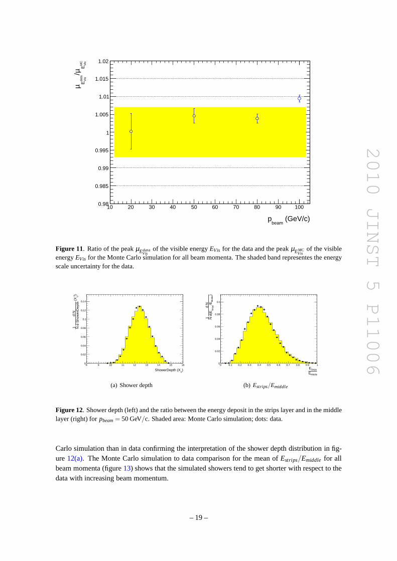
improves whereas the relative beam spread is constant with beam momentum. In addition, the tailstowards lower energies are larger in data than in the Monte Carlo simulation. The same behaviourhas been found for runs of the CTB 2004 without magnetic field [14, 38]. The reason for thisis that the beam line is not modeled in the Monte Carlo simulation and the beam line acceptanceweighting does only approximate the effect of the beam line.In order to quantify this effect,the visible energyEVis distributions are fitted with Crystal Ball functions12 and thetail fractionis defined as the fraction of events with a visible energyEVis below the meanµEVis of the fittedCrystal Ball function minus two standard deviationsσEVis of the fitted Crystal Ball function. Thetail fraction for Monte Carlo simulation and data is shown intable3 for all beam momenta. Notethat for a Gaussian distribution the tail fraction would be 2.3%.

The ratio of the peakµEdataVis

for the data and the peakµEMCVis

for the Monte Carlo simulation isshown in figure11 for all beam momenta. The deviation ofµEdata

calib/µEMC

calibfrom 1 is compatible with

the energy scale uncertainty and the error bars. The main contributions to the error bars are thebeam momentum uncertainty (data only) and the statistical errors.

12The definition of the Crystal Ball function is given in section 7.1, eq. (7.5).

– 16 –

2010 JINST 5 P11006

(GeV)PSE

-1 -0.5 0 0.5 1 1.5 2 2.5 3 3.5 4

)-1

(G

evP

SdEd

N

N1

0

0.02

0.04

0.06

0.08

0.1

0.12

(a) Presampler

(GeV)StripsE

0 5 10 15 20 25 30

)-1

(G

evS

trip

sdE

d N

N1

0

0.02

0.04

0.06

0.08

0.1

0.12

0.14

(b) Strip layer

(GeV)MiddleE

0 5 10 15 20 25 30 35 40 45 50

)-1

(G

evM

iddl

edE

d N

N1

0

0.02

0.04

0.06

0.08

0.1

0.12

0.14

(c) Middle layer

(GeV)BackE

-0.2 0 0.2 0.4 0.6 0.8 1

)-1

(G

evB

ack

dEd

N

N1

0

0.02

0.04

0.06

0.08

0.1

0.12

0.14

0.16

0.18

(d) Back layer

Figure 9. Energy deposit in all layers forpbeam= 50 GeV/c. Shaded area: Monte Carlo simulation; dots:data.

Table 3. Tail fraction (defined in the text) for Monte Carlo simulation and data for all beam momenta.

pnominalbeam Tail fraction Tail fraction

(GeV/c) Data (%) Monte Carlo simulation (%)

20 16.0(6) 10.8(2)50 16.0(3) 11.9(2)80 16.2(5) 8.5(1)100 14.4(3) 6.4(1)

3.4.3 Shower development

For the comparison of the longitudinal shower development two quantities are studied. Since inboth quantities reconstructed energies appear in the numerator as well as in the denominator, theyare independent of the global energy scale. The first quantity is the shower depthXmeandefined asthe energy weighted average layer depth of all accordion layers by

Xmean=EStripsXStrips+EMiddleXMiddle +EBackXBack

EStrips+EMiddle+EBack, (3.3)

– 17 –

2010 JINST 5 P11006

(GeV)VisE

14 15 16 17 18 19 20 21 22

)-1

(G

evV

isdEd

N

N1

0

0.02

0.04

0.06

0.08

0.1

(a) pbeam= 20 GeV/c

(GeV)VisE

38 40 42 44 46 48 50 52 54

)-1

(G

evV

isdEd

N

N1

0

0.02

0.04

0.06

0.08

0.1

0.12

0.14

0.16

0.18

0.2

0.22

(b) pbeam= 50 GeV/c

(GeV)VisE

65 70 75 80 85

)-1

(G

evV

isdEd

N

N1

0

0.05

0.1

0.15

0.2

0.25

(c) pbeam= 80 GeV/c

(GeV)VisE

85 90 95 100 105 110

)-1

(G

evV

isdEd

N

N1

0

0.05

0.1

0.15

0.2

0.25

(d) pbeam= 100 GeV/c

Figure 10. Total LAr EM calorimeter responseEVis (sum of the accordion compartments plus presamplerlayer) for all beam momenta. Shaded area: Monte Carlo simulation; dots: data.

Table 4. LAr EMB layer boundaries and average depth at the beam impact point (η = 0.442,ϕ = 0).

Layer Xstartlayer (X0) Xstop

layer (X0) Xlayer (X0)

Presampler 1.50 1.78 1.64Strips 2.18 6.41 4.29

Middle 6.41 25.02 15.71Back 25.02 26.78 25.90

whereXStrips,XMiddle,XBack denote the average depth of the corresponding layer in unitsof radi-ation lengths (X0) given in table4. The Monte Carlo simulation to data comparison is shown infigure12(a)for pbeam= 50 GeV/c. Again there is sufficiently good agreement, although the simu-lated showers tend to be shorter with respect to the data.

The second quantity for the longitudinal shower development is the ratioEstrips/Emiddle of theenergies of the strip and middle layers. This ratio is very sensitive to the amount of material in frontof the calorimeter. Therefore it can be used to assess the level of accuracy of the material descrip-tion in the simulation. The Monte Carlo simulation to data comparison is shown in figure12(b)for pbeam= 50 GeV/c. The shape agreement is good. Again, the showers start earlier in the Monte

– 18 –

2010 JINST 5 P11006

(GeV/c)beam

p

10 20 30 40 50 60 70 80 90 100

Vis

MC

Eµ/V

isda

taEµ

0.98

0.985

0.99

0.995

1

1.005

1.01

1.015

1.02

Figure 11. Ratio of the peakµEdataVis

of the visible energyEVis for the data and the peakµEMCVis

of the visibleenergyEVis for the Monte Carlo simulation for all beam momenta. The shaded band representes the energyscale uncertainty for the data.

)0

ShowerDepth (X

8 9 10 11 12 13 14 15 16

)-1 0

(X

d S

how

erD

epth

d N

N1

0

0.02

0.04

0.06

0.08

0.1

0.12

0.14

(a) Shower depth

MiddleEStripsE

0 0.1 0.2 0.3 0.4 0.5 0.6 0.7 0.8 0.9 1

)M

iddl

e/E

Str

ips

d(E

d N

N1

0

0.02

0.04

0.06

0.08

0.1

(b) Estrips/Emiddle

Figure 12. Shower depth (left) and the ratio between the energy deposit in the strips layer and in the middlelayer (right) forpbeam= 50 GeV/c. Shaded area: Monte Carlo simulation; dots: data.

Carlo simulation than in data confirming the interpretationof the shower depth distribution in fig-ure 12(a). The Monte Carlo simulation to data comparison for the mean of Estrips/Emiddle for allbeam momenta (figure13) shows that the simulated showers tend to get shorter with respect to thedata with increasing beam momentum.

– 19 –

2010 JINST 5 P11006

(GeV/c)beam

p

10 20 30 40 50 60 70 80 90 100

>M

CM

iddl

eE

MC

Str

ips

E>

/ <

data

Mid

dle

E

data

Str

ips

E<

0.95

0.96

0.97

0.98

0.99

1

1.01

1.02

1.03

1.04

1.05

Figure 13. Ratio of the mean of the ratio between the energy deposit in the strips layer and in the middle

layer

⟨Edata

strips

Edatamiddle

⟩

for the data and

⟨EMC

strips

EMCmiddle

⟩

for the Monte Carlo simulation for all beam momenta.

3.4.4 Systematic uncertainties

The level of accuracy of the Monte Carlo simulation description of the electromagnetic showerdevelopment in the LAr calorimeter is affected by uncertainties associated with the geometricalset-up and detector description (thickness of the lead absorbers, the depth of the first layer, theexact amount of material in front of the strip compartment, cables, electronics, the thickness ofthe cryostat and the amount of LAr in front of the presampler). Similar uncertainties will be anissue for the ATLAS detector at the LHC. Therefore, it is important to investigate them in thecontrolled test-beam environment. However, the uncertainties associated with the description ofthe combined test beam set-up itself will not be present in ATLAS. In order to understand the truesystematic effects relevant to ATLAS, the combined test beam set-up-related uncertainties must beunderstood and a procedure developed to isolate them.

The dominant contributions of the total systematic uncertainty are

• Uncertainties in the knowledge of the beam momentum. Although the absolute beam mo-mentum may include large errors, the relative momentum shifts between different nominalbeam momenta are considerably smaller and depend on changesin beam conditions (colli-mator apertures, magnet currents, etc). Their total contribution is generally relatively smallat the level of 0.1 % (0.2 % for a beam momentum of 20 GeV/c and below) [14].

• Simulation uncertainties in the description of the electromagnetic shower development bythe simulation. Comparisons betweenGEANT4.8 andGEANT4.7 showed small differences

– 20 –

2010 JINST 5 P11006

at the level of 1% in the lateral and longitudinal shower development because GEANT 4.8features an improved description of multiple Coulomb scattering.

• Uncertainties in the Monte Carlo simulation description ofthe beam line and the descriptionof the cryostat and the calorimeter. The impact of these contributions on the uncertaintyof the reconstructed energy is smaller than 0.4 %. However, in terms of linearity, the listedeffects have a much larger impact at lower energies than at higher energies; their impacton the linearity for momenta> 20 GeV/c is estimated to be less than 0.1 %. Most of themcome from the limited precision of the measurement of some parameters like the beam-linegeometry, detector geometry, cross-talk, etc. These uncertainties — except uncertainties ofthe beam-line description — will also be present for ATLAS and are therefore listed below:

– Cross-talk in the strip compartment

– MPhys/MCal in the strip compartment (see subsection3.3.1)

– Cross-talk between the strip and middle compartments

– Depth of the strip section (boundary between middle and strip compartment)

– Lead absorber thickness

– Monte Carlo simulation description of the presampler response

– Upstream material in the beam line

– Material in front of the presampler

– Dead material between the presampler and the strip compartment

– Simulation of charge collection

– Monte Carlo simulation description of lateral and longitudinal shower shape

A detailed description of the systematic uncertainties canbe found in [14].

3.5 The Calibration Hits Method

In the LAr calorimeter only energy deposits inside the active material of the calorimeter are mea-sured. This implies that certain energy deposits are not measured directly. These are

1. Energy deposited outside the electromagnetic calorimeter: In the Monte Carlo simulationthis energy is split into 3 contributions:

• EtrueupstreamPS: Energy deposited upstream of the presampler, see section3.5.2.

• EtruePS−Acc: Energy deposited between the presampler and the accordion, see section3.5.2.

• Etruedownstream: Energy deposited downstream of the accordion, see section3.5.4.

2. Energy deposited inside the electromagnetic calorimeter, but outside of the reconstructedcluster: In order to minimize the noise contribution and to be able to measure the energies ofseveral particles simultaneously, clusters of finite size are used for the energy measurement.However, the energy deposits in the calorimeter cells outside the cluster are not taken directlyinto account and therefore have to be estimated, see section3.5.3.

– 21 –

2010 JINST 5 P11006

3. Energy deposited inside the reconstructed cluster in theinactive material: Because the LArEMB calorimeter is a sampling calorimeter and the development and energy deposition ofthe electromagnetic cascade for an electron is a stochasticprocess, the ratio of the energydeposits in the active and passive material inside the cluster varies event-by-event and also asa function of the beam momentum. At 0th order this ratio is approximated by a single factor,thesampling fraction, which is already applied at the cell reconstruction level.Higher ordercorrections are presented in subsection3.5.3.

These energy deposits are recorded as additional hits in thesimulation, therefore the nameCali-bration Hits Method.

The idea of this calibration procedure is to estimate these different kinds of energy depositsby means of Monte Carlo simulations and correlate them to measurable quantities, namely themeasured cluster presampler energyEPS, the measured cluster accordion energyEAcc which is thesum of the strips, middle and back layer cluster energies,

EAcc = EStrips+EMiddle+EBack, (3.4)

or the shower depthXmean. Therefore quantities for the different energy deposits are defined foreach event. These quantities are binned with respect to the measurable quantity that is used toparameterize the energy deposits. For each bin a representative value is computed. Finally a fit tothese extracted representative values is made in order to obtain the desired parameterization for theestimate.

The performance of theCalibration Hits Methodfor the Combined Test Beam 2004 for runswithout magnetic field in the Inner Detector has already beendiscussed in [14, 38]. Therefore,the impact of the presence of the magnetic field in the Inner Detector on the performance of theCalibration Hits Methodwill be emphasized.

3.5.1 General strategy for the computation of representative values for distributions

The calibration of the electron energy is performed with respect to the peak position of the cali-brated cluster energy. The reason for this choice is to minimize the effect of event selection cutsfor physics analyses. These cuts mostly affect events in thetails of the various distributions and thedependence of peak values on these tails is the small. In order to be consistent, the peak positionof a distribution is used to characterize its representative value throughout this section.

3.5.2 Estimation of the energy deposited upstream of the accordion

The energy deposited upstream of the accordion consists of the energy deposited upstream of thepresamplerEtrue

upstreamPS, the energy deposited in the presamplerEtruePS and the energy deposited be-

tween the presampler and the accordionEtruePS−Acc. For a given beam momentum the sum of these en-

ergies, denotedEtrueupstreamAccis estimated as a function of the measured presampler energyEPS. For

bins ofEPS covering the whole energy range of presampler energy measurements, theEtrueupstreamAcc

distributions are accumulated.For each bin a fit with a Gaussian is performed around the peak and the mean of the Gaussian

EtrueupstreamAccis attributed to the measured presampler energy corresponding to the center of the bin.

The resulting profile is plotted in figure14 for pbeam= 50 GeV/c.

– 22 –

2010 JINST 5 P11006

(GeV)PSE

0 0.2 0.4 0.6 0.8 1 1.2 1.4 1.6 1.8 2

(G

eV)

upst

ream

Acc

true

E

0.5

1

1.5

2

2.5

Figure 14. Energy deposited upstream of the accordion as a function ofthe reconstructed presampler energyfor pbeam= 50 GeV/c. The error bars are within the disks.

(GeV/c)beam

p

20 30 40 50 60 70 80 90 100

(G

eV)

a

0.425

0.43

0.435

0.44

0.445

0.45

(GeV/c)beam

p

20 30 40 50 60 70 80 90 100

b

1.02

1.04

1.06

1.08

1.1

Figure 15. Offset (left) and slope (right) of the estimation of the energy deposited upstream of the accordion(eq. (3.5) and eq. (3.6)).

For each beam momentum a straight line is fitted. The obtainedoffsetsa(pbeam) and slopesb(pbeam) are shown in figure15. For the runs at the Combined Test Beam 2004 without magneticfield in the Inner Detector the offsets ¯a(pbeam) are a monotonously rising function ofpbeam [38].With magnetic field in the Inner Detector, the tracks of the particles with lower momentum arebent more strongly resulting in a smaller impact angle. Thisleads to an increase of the lengths ofthe tracks in the cryostat and therefore to an increase of ¯a(pbeam). As a consequence, the obtainedoffsetsa(pbeam) are a nearly constant function ofpbeamwithin the errors.

– 23 –

2010 JINST 5 P11006

Next, the offset as a function of the beam momentum is parameterized by fitting

a(pbeam) = a0 +a1 logpbeam, (3.5)

and the slope by fittingb(pbeam) = b0 +b1 logpbeam, (3.6)

with pbeam in units of GeV c−1 for the logarithms. These are the same parameterizations that havealso been used for the runs without magnetic field in the InnerDetector. The slope is very wellparameterized and the differences for the offset are at the level of 20 MeV. The fitted values area0 = 0.45(1) GeV,a1 = −0.003(3) GeV,b0 = 0.89(2) GeV andb1 = 0.43(5) GeV.

Then for a given event at a given beam momentum the energy deposited upstream of theaccordion is estimated by

EestimupstreamAcc(EPS, pbeam) = a(pbeam)+ b(pbeam)EPS. (3.7)

In order to determine the particle energy without prior knowledge of the beam momentum, aniterative procedure is applied, see subsection3.5.5.

3.5.3 Estimation of the energy deposited in the accordion

The energyEtrueAcc deposited in the accordion can be estimated either as a function of the shower

depth or as a function of the beam momentum.For each event the ratiod of the energy deposited in the accordion and the measured accordion

energy (equation (3.4)) is defined by

d =Etrue

Acc

EAcc. (3.8)

Beam momentum parameterization. For each beam momentum a Gaussian is fitted to the ddistribution for the specific beam momentum and the mean of this Gaussiand(pbeam) is extractedand shown in figure16. Thend(pbeam) is approximated by fitting

d(pbeam) = d0 +d1 logpbeam+d2 (log pbeam)2 , (3.9)

with pbeam in units of GeV c−1 for the logarithms. The fitted values ared0 = 1.262516(15), d1 =

0.107626(8) andd2 = 0.011840(1).The values ford are close to one since a coarse sampling fraction correctionis applied at the

cell energy reconstruction (FµA→MeV, see section3.3.1). It increases with decreasing beam mo-mentum because of two effects: The sampling fraction slightly decreases with decreasing beammomentum [39] and this is not taken into account by the coarse sampling fraction correction men-tioned above. In addition, since the electrons are strongerdeflected by the magnetic field withdecreasing beam momentum, the emitted bremsstrahlung is more likely to be not contained in thecluster which increases the fraction of energy deposited outside the cluster with decreasing beammomentum.

For a given event at a given beam momentum the energy deposited in the accordion is esti-mated by

EestimAcc (EAcc, pbeam) = d(pbeam)EAcc. (3.10)

In order to determine the particle energy without prior knowledge of the beam momentum, aniterative procedure is applied, see subsection3.5.5.

– 24 –

2010 JINST 5 P11006

(GeV/c)beam

p

20 30 40 50 60 70 80 90 100

d

1

1.01

1.02

1.03

1.04

1.05

1.06

1.07

1.08

1.09

1.1

Figure 16. Meand(pbeam) of the Gaussian fitted to the d distribution (eq. (3.8)) for all beam momenta andits parameterizationd(pbeam). The error bars are within the disks.

Shower depth parameterization. The idea of this parameterization is to correct for samplingfraction fluctuations event by event by relating the sampling fraction to the shower depth. Analysesof CTB 2004 data have shown that this method works very well without magnetic field upstreamof the calorimeter [14].

For bins of the measured shower depthXmeancovering the whole shower depth range, theddistributions are accumulated. For each bin a fit with a Gaussian is performed and the mean of theGaussiand(Xmean) is attributed to the measured shower depth corresponding tothe center of thebin. The resulting profiles for all beam momenta are shown in figure17.

Figure17demonstrates that the parameterization ofd(Xmean) as a function of the shower depthdoes not remove the dependence on the beam momentum. This is contrary to what has been foundfor the Combined Test Beam 2004 for runs without magnetic field in the Inner Detector [14, 38].The reason for this discrepancy is that in the presence of themagnetic field the energy depositedinside the electromagnetic calorimeter but outside of the reconstructed cluster relative to the energyof the particle depends on the beam momentum. In figure18 the meand5x11(pbeam) dependencefor clusters of 5×11 instead of 3×7 middle cells (section3.3.2) is shown for all beam momenta.These clusters are large enough to contain the whole shower in the calorimeter. The fact that there isno beam momentum dependence for the 5×11 clusters indicates that the 3×7 cluster size togetherwith the magnetic field generates the dependence ofd(Xmean) on the beam momentum. Thereforethis parameterization is not used for the linearity and resolution measurements in section3.6.

The same effect is also visible in ATLAS Monte Carlo simulation, although the effect there is

– 25 –

2010 JINST 5 P11006

)0

(XmeanX

8 9 10 11 12 13 14 15 16

d

1

1.01

1.02

1.03

1.04

1.05

1.06

1.07

1.08

1.09

1.1= 20 GeV/c

beamp

= 50 GeV/cbeam

p

= 80 GeV/cbeam

p

= 100 GeV/cbeam

p

Figure 17. Meand(pbeam) of the Gaussian fitted to the d distribution (equation (3.8)) as a function of theshower depthXmeanfor all beam momenta.

so small that the shower depth parameterization is used by default for the electron energy calibra-tion [40]. The reason why this effect is much smaller for the ATLAS detector is that the geometriclayout of the CTB 2004 is a bit different from ATLAS, in particular the distances between the innerdetector components and the LAr EMB calorimeter are larger for the CTB 2004 setup.

3.5.4 Estimation of the energy deposited downstream of the accordion

The energyEtruedownstreamdeposited downstream of the accordion can be estimated either as a function

of the shower depth or as a function of the beam momentum.

Beam momentum parameterization. For each beam momentum a Gaussian is fitted to theEtrue

downstreamdistribution and the mean of the GaussianEtruedownstream(pbeam) is obtained and shown

in figure19. ThenEtruedownstream(pbeam) is approximated by fitting

Eestimdownstream(pbeam) = λ0 pbeam+ λ1 p2

beam. (3.11)

The fitted values areλ0 = 9(4)10−4 c andλ1 = 2.3(7)10−6 c2 GeV−1.

In order to determine the particle energy without prior knowledge of the beam momentum, aniterative procedure is applied, see section3.5.5.

Shower depth parameterization. For each event the ratio of the energy deposited downstreamof the accordion and the measured accordion energy which is the sum of the measured strips,

– 26 –

2010 JINST 5 P11006

)0

(XmeanX

8 9 10 11 12 13 14 15 16

5x11

d

0.99

0.995

1

1.005

1.01

1.015

1.02

1.025

1.03= 20 GeV/c

beamp

= 50 GeV/cbeam

p

= 80 GeV/cbeam

p

= 100 GeV/cbeam

p

Figure 18. Meand5x11(pbeam) of the Gaussian fitted to the d distribution (equation (3.8)) for 5×11 clustersas a function of the shower depthXmeanfor all beam momenta.

middle and back layer energies is defined by

λ =Etrue

downstream

EAcc. (3.12)

For bins of the measured shower depthXmean covering the whole shower depth range, theλ distributions are accumulated. For each bin a fit with a Gaussian is performed and the mean ofthe Gaussianλ (Xmean) is attributed to the measured shower depth corresponding tothe center ofthe bin. The resulting profiles for all beam momenta are plotted in figure20.

Figure20 shows that the parameterization of the ratio of energy deposited downstream of theaccordion and the measured accordion energy does not completely remove the dependence on thebeam momentum. The remaining differences are at the half permille level.

For the reasons shown in section3.5.3, this parameterization is not used for the linearity andresolution measurements in section3.6.

3.5.5 Iterative procedure

An iterative procedure is applied to compute the calibratedcluster energy. Starting value for theestimate for the calibrated cluster energy is the visible energy. In each iteration step the estimatedcalibrated cluster energy from the previous step together with

E2 = p2c2 +m2c4 (3.13)

– 27 –

2010 JINST 5 P11006

(GeV/c)beam

p

20 30 40 50 60 70 80 90 100

(G

eV)

dow

nstr

eam

true

E

0

0.05

0.1

0.15

0.2

0.25

0.3

0.35

Figure 19. Mean of the energy deposited downstream of the accordion for all beam momenta and its param-eterizationEestim

downstream(pbeam) (eq. (3.11)).

is used to estimate the proper beam/particle momentum to select the new estimation coefficients.Here the knowledge that electrons have been selected from the beam is used to justify the neglectof the rest mass term contribution to the particle energy.13 The selected estimation coefficients arethen used to compute a new estimate for the calibrated cluster energy.

Beam momentum parameterization. Using the beam momentum parameterizations for the en-ergy Eestim

Acc deposited in the accordion and the energyEestimdownstreamdeposited downstream of the

accordion, the iterative procedure is given by:

E0Calib = EPS+EAcc

p0 =E0

Calib

c...

EkCalib = Eestim

upstreamAcc(EPS, pk−1)+EestimAcc (EAcc, pk−1)

+Eestimdownstream(pk−1)

= a(pk−1)+ b(pk−1)EPS+ d(pk−1)EAcc

+Eestimdownstream(pk−1) k > 0

pk =Ek

Calib

ck > 0 (3.14)

13The rest mass of an electron isme = 511 keV/c. The investigated beam momenta are> 10 GeV/c.

– 28 –

2010 JINST 5 P11006

)0

(XmeanX

8 9 10 11 12 13 14 15 16

λ

0

0.001

0.002

0.003

0.004

0.005

0.006

0.007

0.008

0.009

0.01= 20 GeV/c

beamp

= 50 GeV/cbeam

p

= 80 GeV/cbeam

p

= 100 GeV/cbeam

p

Figure 20. Meanλ(pbeam) of the Gaussian fitted to theλ distribution (equation (3.12)) as a function of theshower depthXmeanfor all beam momenta.

where pk is the k-th estimation of the particle momentum andEkCalib is the k-th estimation of

the particle energy.EestimupstreamAcc(EPS, pk−1) = a(pk−1)+ b(pk−1)EPS is used to estimate the energy

deposited upstream of the accordion andEestimAcc (EAcc, pk−1) = d(pk−1)EAcc to estimate the energy

deposited in the accordion.

This iteration procedure is executed until the relative difference between the two consecutiveECalib values|Ek

Calib−Ek−1Calib| is smaller than 10−6. On average 3 iterations are required to meet this

termination condition.

3.6 Linearity and resolution

The calibrated cluster energies are computed using the iteration scheme for the beam momentumparameterization (eq. (3.14)). The Monte Carlo simulation to data comparison is shown infigure21for all beam momenta. The shape agreement for calibrated cluster energy distributions is similar tothe shape agreement for the visible energy distributions described in section3.4.2. This means thatthe shape agreement is best atpbeam= 20 GeV/c and deteriorates with increasing beam momentumdue to the beam spread that has not been simulated and due to low energy tails larger in data than inthe Monte Carlo simulation. These low energy tails are mainly due to the fact that a priori the beamparticles are simulated without taking into account any losses along the beam line. The correctionintroduced in section3.4.1only describes this effect in an approximate manner.

The calibrated cluster energy distributions are fitted withCrystal Ball functions14 and the mean

14The definition of the Crystal Ball function is given in section 7.1, eq. (7.5).

– 29 –

2010 JINST 5 P11006

(GeV)CalibE

14 15 16 17 18 19 20 21 22

)-1

(G

evC

alib

dEd

N

N1

0

0.02

0.04

0.06

0.08

0.1

(a) pbeam= 20 GeV/c

(GeV)CalibE

38 40 42 44 46 48 50 52 54

)-1

(G

evC

alib

dEd

N

N1

0

0.02

0.04

0.06

0.08

0.1

0.12

0.14

0.16

0.18

0.2

0.22

(b) pbeam= 50 GeV/c

(GeV)CalibE

65 70 75 80 85

)-1

(G

evC

alib

dEd

N

N1

0

0.05

0.1

0.15

0.2

0.25

(c) pbeam= 80 GeV/c

(GeV)CalibE

85 90 95 100 105 110

)-1

(G

evC

alib

dEd

N

N1

0

0.05

0.1

0.15

0.2

0.25

(d) pbeam= 100 GeV/c

Figure 21. Calibrated energy for all beam momenta. Shaded area: MonteCarlo simulation; dots: data.

µEcalib and the sigmaσECalib of these Crystal Ball functions divided byEbeam= pbeam·c are plottedin figure22and figure23 to assess the linearity and resolution.

In figure 22 the deviation ofµEcalib/Ebeam from 1 is within the energy scale uncertainty andthe error bars. The main contributions to the errors bars arethe beam momentum uncertainty (dataonly) and the statistical errors. The square root of the meansquared deviation ofµEcalib/Ebeamfrom1 is 0.1% for the Monte Carlo simulation and 0.6% for the data.For the data this is within theenergy scale uncertainty. Adjusting the energy scale, the linearity defined as the unbiased estimateof the standard deviation ofµEcalib/Ebeamis 0.1% for the Monte Carlo simulation and 0.28% for thedata. This is within the estimated systematic uncertainties discussed in section3.4.4. Therefore thelinearity at the CTB 2004 is understood at the level of the estimated systematic uncertainties.

The resolution shown in figure23 is described by

σECalib(Ebeam)

Ebeam=

a√Ebeam

⊕ bEbeam

⊕c (3.15)

where the first term in the quadratic sum is the stochastic term, the second the noise term andthe third the local constant term. Since the beam spreadσ(pbeam) (table 1) was not simulated,it have been subtracted quadratically for every measurement point for Data in figure23 before.In addition, since the noise of the read-out electronics wasmeasured regularly during the whole

– 30 –

2010 JINST 5 P11006

(GeV/c)beam

p

10 20 30 40 50 60 70 80 90 100

beam

EC

alib

Eµ

0.98

0.985

0.99

0.995

1

1.005

1.01

1.015

1.02

Data

Monte Carlo simulation

Figure 22. Linearity for Monte Carlo simulation and data. The shaded band representes the energy scaleuncertainty for the data.

CTB 2004 data taking period by taking dedicated calibrationruns, the noise values for the 3x7clusters have also been subtracted quadratically for everymeasurement point for Data in figure23before. They have been computed for each run by averaging thenoise values for the clusters overevents that have been triggered randomly. The noise value ofa given cluster was computed as thequadratic sum of the noise values of all cells in the cluster in their chosen read out gain for thegiven event. The noise value of a given cell in a given read outgain was taken from the previouslymentioned calibration runs. The noise values are shown in table 5. The noise increases slightlywith increasing beam momentum because more cells are read out in medium gain than in high gaindue to the higher energy deposits and because the noise for the medium gain is higher than forthe high gain. The reason for this difference in the noise values of a cell for the various gains isthat the noise is first amplified with different gain factors but then digitized with a constant ADCresolution. Afterwards the gain dependentFDAC→µA ·FµA→MeV factor (see section3.3.1) is appliedto adjust the mean values of the noise distributions for the different gains. The net result of thisprocedure on the standard deviation of the noise distribution of a given cell which is the noise valueof the given cell is the small gain dependence.

The error bars for the resolution shown in figure23 are dominated by the systematic errorof the fit of the calibrated cluster energy distributions from figure21. The error bars have beenestimated to be the difference of the standard deviations obtained with three different models: AGaussian fitted to the peak part of the distribution, a Crystal Ball function fitted to the distributionand an exponential function convoluted with a Gaussian (defined by equation (7.3)) fitted to thedistribution.

– 31 –

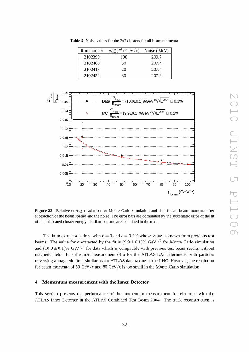
2010 JINST 5 P11006

Table 5. Noise values for the 3x7 clusters for all beam momenta.

Run number pnominalbeam (GeV/c) Noise (MeV)

2102399 100 209.72102400 50 207.42102413 20 207.42102452 80 207.9

(GeV/c)beam

p

10 20 30 40 50 60 70 80 90 100

beam

EC

alib

Eσ

0

0.005

0.01

0.015

0.02

0.025

0.03

0.035

0.04

0.045

0.05

0.2%⊕ beamE/1/20.1)%GeV± = (10.0beamE

CalibEσData

0.2%⊕ beamE/1/20.1)%GeV± = (9.9beamE

CalibEσMC

Figure 23. Relative energy resolution for Monte Carlo simulation anddata for all beam momenta aftersubtraction of the beam spread and the noise. The error bars are dominated by the systematic error of the fitof the calibrated cluster energy distributions and are explained in the text.

The fit to extracta is done withb = 0 andc = 0.2% whose value is known from previous testbeams. The value fora extracted by the fit is(9.9± 0.1)% GeV1/2 for Monte Carlo simulationand (10.0± 0.1)% GeV1/2 for data which is compatible with previous test beam resultswithoutmagnetic field. It is the first measurement ofa for the ATLAS LAr calorimeter with particlestraversing a magnetic field similar as for ATLAS data taking at the LHC. However, the resolutionfor beam momenta of 50 GeV/c and 80 GeV/c is too small in the Monte Carlo simulation.

4 Momentum measurement with the Inner Detector

This section presents the performance of the momentum measurement for electrons with theATLAS Inner Detector in the ATLAS Combined Test Beam 2004. The track reconstruction is

– 32 –

2010 JINST 5 P11006

described in section4.1. This is followed by a comparison of the Monte Carlo simulation to data(section4.2). The data samples and the event selection were the same as insection3.

4.1 Track reconstruction

The track reconstruction algorithms for the CTB 2004 have been implemented in the CTB-Tracking(‘Cosmics + TestBeam’) package. This package provides a pattern recognition that works without avertex constraint which is an ideal approach for the testbeam and is also needed for other situations,e.g. reconstructing cosmic or beam halo events. Details canbe found in [41].

Tracks in the Inner Detector are reconstructed in three consecutive steps. In the pre-processingstep, the raw data from the Pixel and SCT detectors are converted into clusters and the SCT clustersare then transformed into space-points. Furthermore, the TRT raw timing information is, based ona calibration obtained from data, first corrected for an offset with respect to the expected timeof a signal for particles passing through the middle of the straw, and then the remaining delaycaused by drift time is converted into a drift radius. At the track-finding step track candidates areidentified using different tracking strategies. Fake tracks among these track candidates are rejectedby applying quality cuts, e.g. on the number of associated clusters or the number of holes pertrack (a hole is defined as a silicon sensor crossed by a track without generating any associatedcluster). The remaining track candidates are the reconstructed tracks for the given event. The trackparameters are determined by globalχ2 minimization of the residuals (i.e. the difference betweenthe measurement position and the position as predicted by the track), and their errors. During thefinal post-processing stage photon conversions and secondary vertices are reconstructed. At theCTB this final step is of minor importance except for photon conversion studies.

In a homogeneous magnetic field the sagitta of a curved track is directly proportional to 1/pand without bremsstrahlung events would be distributed like a Gaussian. The resolution of theinverse transverse momentum 1/pT (which is equal to the inverse momentum in the CTB) can beexpressed as a function ofpT :

σ1/pT(pT) = σ1/pT

(∞)

(

1⊕ pXT

pT

)

, (4.1)

whereσ1/pT(∞) is the asymptotic resolution expected at infinite momentum and pX

T is a constantrepresenting the value ofpT , for which the contribution of the intrinsic and multiple-scatteringterms to the resolution are equal. Therefore the inverse momentum 1/p measured by the InnerDetector is used in section4.2 to assess the quality of the description of the data by the MonteCarlo simulation. It is normalized to the beam momentumpbeam, i.e. pbeam/p is shown.

4.2 Monte Carlo simulation and comparison with data

The ratiopbeam/p of the beam momentum and the momentum measured by the Inner Detector isshown in figure24 for all beam momenta and compared to Monte Carlo simulation.

The agreement of the description of the tails of the distribution is sufficiently good, but thescale agreement is not better than a few percent because of residual misalignment between thevarious Inner Detector components that could not be resolved [42].

– 33 –

2010 JINST 5 P11006

pbeam

p0 0.5 1 1.5 2 2.5 3

pbeam

pd

d N

N1

0

0.05

0.1

0.15

0.2

0.25

(a) pbeam= 20 GeV/c

pbeam

p0 0.5 1 1.5 2 2.5 3

pbeam

pd

d N

N1

0

0.02

0.04

0.06

0.08

0.1

0.12

0.14

(b) pbeam= 50 GeV/c

pbeam

p0 0.5 1 1.5 2 2.5 3

pbeam

pd

d N

N1

0

0.02

0.04

0.06

0.08

0.1

0.12

(c) pbeam= 80 GeV/c

pbeam

p0 0.5 1 1.5 2 2.5 3

pbeam

pd

d N

N1

0

0.01

0.02

0.03

0.04

0.05

0.06

0.07

0.08

0.09

(d) pbeam= 100 GeV/c

Figure 24. Ratio pbeam/p of the beam momentum and the momentum measured by the Inner Detector forvarious beam momenta. Shaded area: Monte Carlo simulation;dots: data.

5 Particle identification with the Transition Radiation Tra cker

This section presents the electron identification (ePID) with the TRT. After a short introductionto particle identification with the TRT in section5.1, the data samples used for this analysis arediscussed in section5.2. Section5.3 presents methods used for ePID in the TRT, and finally themeasurement of the transition radiation onset from data is discussed in section5.4.

5.1 Introduction to particle identification with the Transi tion Radiation Tracker

The TRT is a straw tube tracker with ePID capabilities mainlythrough detection of transitionradiation photons created in the radiator between the straws. The detector is situated in front ofthe EM calorimeter and is described in detail in [3].

The output of the TRT is 27 bits per straw — 24 low threshold (LT) bits and 3 high threshold(HT) bit spanning 75ns. An illustration of a regular pulse along with its resulting bit output isshown in figure25.

The number of HT hits are mainly the result of transition radiation (TR) photons, createdwhen charged particles with high gamma factors pass the radiator material15 between the straws.

15Material with rapidly changing dielectric constant (filt structure), creating TR through interference.

– 34 –

2010 JINST 5 P11006

����������������������������������������

����������������������������������������

High Threshold (HT) at 6 keV

Low Threshold (LT) at 300 eV

︸ ︷︷ ︸

Time-over-Threshold (ToT)Time (bits)1 bit = 3.125 ns

Pul

sehe

ight

LT bits

HT bits

|0 0 0 0 0 0 0 1|1 1 1 1 1 1 1 0|0 0 0 0 0 0 0 0|0 1 0

Figure 25. Example of a regular TRT pulse including its LT and HT bit response.

At the energies of the final state particles at LHC, essentially only electrons have such high gammafactors, and thus a HT hit signifies an electron.

The number of LT hits refers to the number of straw hits assigned to a specific track. Inprinciple some straws could be crossed without a LT hit, but this fraction is very low, and will nothave any significant influence on the results. For each LT hit,the number of bits set between thefirst bin (leading edge) and the last bin (trailing edge) yields the Time-over-Threshold (ToT). Sinceelectrons ionize more than pions given a certain path lengthin the straw, a longer ToT signifiesan electron. However, since the difference indE/dx between electrons and pions vanishes at highenergy, the ToT variable is expected to give better separation at low energy.

The separation between electrons and hadrons, mostly pions16 presented in the following isbased primarily on the HT information while the ToT information provides secondary separationmost notably at lower energies. The optimization has been done to maximize the pion rejection(defined asRπ = 1/επ , whereεπ is the pion efficiency) at 90% electron efficiency.

The algorithm should also be efficient at finding (possibly soft) electrons in jets forb-quarktagging, which again requires goode/π separation. Here the TRT plays a central role.

5.2 The combined test beam data

5.2.1 Data samples

In order to get the best knowledge of the energy sensitivity of the e/π separation, the whole beammomentum range from 2 to 180 GeV/c was used. For each beam momentum, only runs withoutB-field and without additional material were used, though theresults were not much affected byB-field and material. In addition, muon runs at 150 and 350 GeV/c were added to the data set

16Here and in the following, “pions” will be used as a generic word for “hadrons”.

– 35 –

2010 JINST 5 P11006

Table 6. Table showing all used runs, with their run-number, beam momentum in GeV/c, B-field in T,average number of LT hits, number of eventsNrun, number of events after selectionNcuts and numbers ofpions, electrons, and muons (Nπ , Ne, Nµ ).

Run pnominalbeam (GeV/c) B(T) 〈LT hits〉 Nrun Ncuts Nπ Ne Nµ

2102115 2 0.00 36.38±0.03 50000 25105 3178 15755 1572102098 3 0.00 37.17±0.03 50000 26873 5547 16684 02102097 5 0.00 37.41±0.03 50000 32316 12092 14190 02102103 9 0.00 37.44±0.02 50000 39649 14134 8369 1132102397 20 0.00 32.83±0.02 50000 41500 2378 31817 2712102410 50 0.00 33.75±0.02 50000 39815 6105 27254 122102454 80 0.00 34.38±0.02 50000 39156 6989 24891 332102398 100 0.00 33.89±0.02 40000 32031 8017 16520 5092102433 150 0.16 36.10±0.02 27219 24683 414 0 215902102434 150 0.16 35.78±0.02 29486 26922 2919 0 213002102461 180 0.00 33.95±0.02 50000 44097 20683 6090 24392102730 350 0.16 35.42±0.01 50000 48589 61 0 460292102731 350 0.16 34.57±0.02 30494 29543 47 0 279322102728 350 1.40 34.57±0.02 46416 45098 62 0 42671

for the measurement of the TR onset (see section5.4). These runs had non-zeroB-field. Duringthe data taking period two TRT geometry configurations were used, coinciding with the choice ofbeam momentum, such that at low beam energy (2, 3, 5, and 9 GeV/c) the lower three modules ofthe TRT were centered to the beam, while at high beam energy (20, 50, 80, 100, and 180 GeV/c)the three upper ones were aligned.

The complete list of runs used in this analysis, including their beam momentumpbeam inGeV/c,B-field in T, material statusM, average number of LT hits, number of events in fileNfile andafter cutsNcuts, and estimated statistics for each particle sample is presented in table6.

5.2.2 Data quality

To ensure single high quality TRT tracks with no interference from other effects, events wererequired to have exactly one global track (i.e. a track seen and matched between the Pixel detector,the SCT, and the TRT) with at least 20 hits in the TRT. In addition a quality assurance is applied toeach TRT straw, requiring that at least 100 identified electrons and pions passed through that straw,that the probability for an electron to make a HT hit (pHT

e ) is at least 50% higher than the same fora pion (pHT

π ), and that the latter is below 12.5% to avoid noisy straws. Straws that do not pass thesecuts (6.1%) are removed from the track, and the requirement of at least 20 hits on track is repeated,excluding about 2% of the tracks.

5.2.3 Electron and pion samples

To obtain large clean samples of electrons and pions separately, a Cherenkov counter17 and theATLAS calorimeters were used for discrimination.

17This detector is only part of the CTB setup, not of the ATLAS detector.

– 36 –

2010 JINST 5 P11006

Table 7. Electron and pion contaminations for the non-TRT separation requirements at beam momenta of 2,3, 5, 9, 20, 50, 80, 100, and 180 GeV/c, respectively. An entry of 0.1×10−6 indicates that the contaminationis at or below this level.

pnominalbeam (GeV/c) 2 3 5 9 20 50 80 100 180

e contamination inπ sample (10−6) 8.4 2.1 0.2 0.1 0.1 0.1 0.1 0.1 0.1π contamination inesample (10−6) 17.1 9.5 4.1 0.1 0.1 1.4 1.9 1.9 0.2

The fraction of energy deposited in the first sampling and theentire cluster in the Liquid Argoncalorimeter, provides very good separation. Additional information is provided by the Cherenkovcounter at lower beam momenta (2-20 GeV/c) and the energy fraction in the Tile calorimeter athigher beam momenta (20-180 GeV/c). Finally, the muon system provides a muon tag, such thatalso clean samples of muons are available for the TR onset analysis.

The selections were obtained through an iterative process,where each variable is consideredin turn, while applying the separating requirements to all the other detectors. This optimisationwas performed at all beam energies, as most separation requirements are momentum dependent.For the study of the TRT ePID, reasonably large samples (> 1000 events) are needed, while at thesame time good purities (< 0.2% contamination) are maintained. Generally, contaminations weremuch smaller, see table7. It was checked that possible correlations would not affectthe resultssignificantly.

5.3 Particle identification methods

5.3.1 The high threshold method

The occurrence of a HT hit in a straw signifies transition radiation (TR), which, in the given mo-mentum range, is essentially only emitted by electrons . However, HT hits can also be producedby other particles, mostly because of Landau fluctuations inthedE/dxand/orδ -rays (atomic elec-trons knocked out), which as a result decreases the separation. Given knowledge of the electronand pion HT hit probabilities,pe

HT,i andpπHT,i , these can be used to calculate the probability for a

track to originate from an electron as follows:

peHT =

∏i peHT,i

∑j = e,π

∏i p jHT,i

, (5.1)

where the product of probabilities is normalised to the probability of all possible particle types (inthis analysis only pions and electrons). It has been checkedthat each straw can be considered anindependent detector, and thus there is no correlation between straws.

The electron and pion HT hit probabilities used in the likelihood have been determined asaverages for each straw and at each beam momentum. This method includes the variations withdepth into the TRT observed. Also variations with distance from the track to the anode have beendetermined, but these are not used in the likelihood, as theyare purely geometrical, and do notprovide additional separation. An example of the HT distribution of likelihoods at 9 GeV/c isshown in figure26.

– 37 –

2010 JINST 5 P11006

Electron probability from HT information0 0.1 0.2 0.3 0.4 0.5 0.6 0.7 0.8 0.9 1

Fra

ctio

n of

eve

nts

−310

−210

−110

1

Electrons

Pions

E = 9 GeV

Figure 26. Distribution of likelihoods obtained from the HT information for electrons (solid) and pions(dashed) at 9 GeV/c.

Finally, the distribution of HT hits on the track (i.e. whether they occur randomly distributedor not) has been considered using the Wald-Wolfowitz run test [43]. No significant deviations fromindependent behavior was found.

5.3.2 The time-over-threshold method

In addition to the HT information, one can consider taking the ToT information into account aswell, and especially at low momenta this is expected to increase the separation.

The ToT is very dependent on the distancer from the track to the anode (this is the informationused by the tracking algorithms), and thus this geometricaleffect has to be taken into account whenconsidering the ToT for ePID. Also, while the ToT momentum dependence is not very pronouncedfor electrons, it does change with momentum for pions due to the stronger momentum dependenceof dE/dx for pions. The larger the momentum, the closerdE/dx for pions gets todE/dx ofelectrons, which thus in turn diminishes the separation between the two, using ToT information.

Given the ToT and the distance from the track to the anoder, a likelihood ratio similar to thatof the HT is calculated as follows:

peToT =

∏i,noHT peToT,i

∑j = e,π

∏i,noHT p jToT,i

, (5.2)

wherein the product of probabilities is normalised to the probability of all possible particle types(pions and electrons). The probabilitiespe

ToT and pπToT are determined as a function of ToT andr

for each beam momentum averaged over all straws (to increasestatistics).

Anticipating the combination of the HT and ToT information,the HT hits are excluded fromthe ToT likelihood to minimize the correlation between the two. It has been checked that theToT information of the straws with HT hits do not carry any significant additional separation.An example of the distribution of likelihoods obtained withthe ToT method not using HT hits at9 GeV/c is shown in figure27.

– 38 –

2010 JINST 5 P11006

Electron probability from ToT information0 0.1 0.2 0.3 0.4 0.5 0.6 0.7 0.8 0.9 1

Fra

ctio

n of

eve

nts

−310

−210

−110 Electrons

Pions

E = 9 GeV

Figure 27. Distribution of likelihoods obtained from the ToT information for electrons (solid) and pions(dashed) at 9 GeV/c.

Electron Efficiency

0.84 0.86 0.88 0.9 0.92 0.94 0.96 0.98 1

Pio

n E

ffici

ency

−210

−110

1

E = 9 GeV

90%

ele

ctro

n ef

ficie

ncy

Time−over−threshold

High−threshold

Combined

Figure 28. π-efficiency versuse-efficiency for ToT methods at 9 GeV/c.

5.3.3 Combined method

Having obtained separating methods using both the HT and theToT information, a combination ofthese is considered to achieve the best pion rejection possible. It was checked that the correlationbetween the two were below 20% at all energies, and thereforethe two variables are combined asfollows:

peall =

peHT pe

ToT

∑j = e,π

p jHT p j

ToT

. (5.3)

Thee/π separation performance resulting from this combination can be seen along with theseparate HT and ToT performances in figure28 at 9 GeV/c, which shows theπ-efficiency as afunction ofe-efficiency. As can be seen from the figure, the HT informationprovides the bulk ofthe separation, while the ToT information gives a significant addition, as also seen in the combinedperformance, which is most performant.

– 39 –

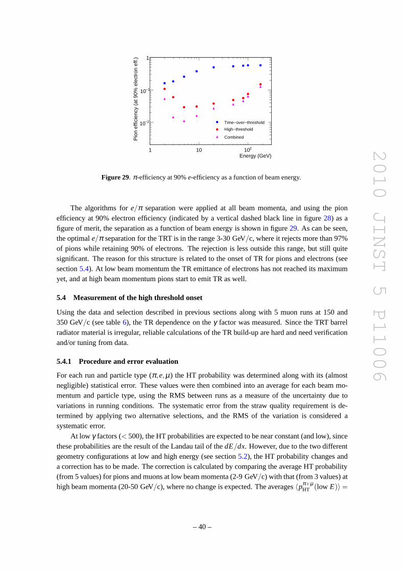
2010 JINST 5 P11006

Energy (GeV)1 10 210

Pio

n ef

ficie

ncy

(at 9

0% e

lect

ron

eff.)

−210

−110

1

Time−over−threshold

High−threshold

Combined

Figure 29. π-efficiency at 90%e-efficiency as a function of beam energy.

The algorithms fore/π separation were applied at all beam momenta, and using the pionefficiency at 90% electron efficiency (indicated by a vertical dashed black line in figure28) as afigure of merit, the separation as a function of beam energy isshown in figure29. As can be seen,the optimale/π separation for the TRT is in the range 3-30 GeV/c, where it rejects more than 97%of pions while retaining 90% of electrons. The rejection is less outside this range, but still quitesignificant. The reason for this structure is related to the onset of TR for pions and electrons (seesection5.4). At low beam momentum the TR emittance of electrons has not reached its maximumyet, and at high beam momentum pions start to emit TR as well.

5.4 Measurement of the high threshold onset

Using the data and selection described in previous sectionsalong with 5 muon runs at 150 and350 GeV/c (see table6), the TR dependence on theγ factor was measured. Since the TRT barrelradiator material is irregular, reliable calculations of the TR build-up are hard and need verificationand/or tuning from data.

5.4.1 Procedure and error evaluation

For each run and particle type (π,e,µ) the HT probability was determined along with its (almostnegligible) statistical error. These values were then combined into an average for each beam mo-mentum and particle type, using the RMS between runs as a measure of the uncertainty due tovariations in running conditions. The systematic error from the straw quality requirement is de-termined by applying two alternative selections, and the RMS of the variation is considered asystematic error.

At low γ factors (< 500), the HT probabilities are expected to be near constant (and low), sincethese probabilities are the result of the Landau tail of thedE/dx. However, due to the two differentgeometry configurations at low and high energy (see section5.2), the HT probability changes anda correction has to be made. The correction is calculated by comparing the average HT probability(from 5 values) for pions and muons at low beam momenta (2-9 GeV/c) with that (from 3 values) athigh beam momenta (20-50 GeV/c), where no change is expected. The averages〈pπ+µ

HT (low E)〉=

– 40 –

2010 JINST 5 P11006

−factor γ

10 210 310 410 510

Hig

h−th

resh

old

prob

abili

ty

00.020.040.060.08

0.10.120.140.160.18

0.20.22

−factor γ

10 210 310 410 510

Hig

h−th

resh

old

prob

abili

ty

00.020.040.060.08

0.10.120.140.160.18

0.20.22

Pion momentum (GeV) 1 10

Muon momentum (GeV)210

Electron momentum (GeV)10 210

Electrons

Muons

Pions

ATLAS TRT barrelCombined test beam data, 2004

Figure 30. HT Probability as a function ofγ factor for electrons (squares), muons (triangles) and pions(circles) in the beam energy range 2-350 GeV/c. The curve is a fit with a generic function, and the fitresiduals are shown in the top plot, where the two dashed lines represent±0.005.

0.0402 and〈pπ+µHT (high E)〉 = 0.0350 compared to the overall average of〈pπ+µ

HT (all E)〉 = 0.0383yield corrections of -0.0020 and 0.0033 at low and high beam momenta, respectively. Half of thecorrections are used as a systematic error.

5.4.2 Results

The final values and their uncertainties are fitted with a generic function of log10γ consisting of afirst degree polynomial and a sigmoid function:

pHT(γ) = c0 +c1 log10γ +c2

1.0+exp(−(log10γ −c3)/c4)(5.4)

with γ ∈ [1,500000]. The result, along with the data points and the fitted function, can be seen infigure30.

As figure30 shows, the fit describes the data well. Inγ regions in figure30 where the valuesfor the different particle types overlap, the HT probability does not seem to depend on the particletype, but only on theγ factor, as expected.

While the HT onset starts at aboutγ ∼ 1000, it does not reach its maximum untilγ ∼ 15000.Likewise, even at high beam momenta pions do not emit much TR,and can thus be separatedfrom electrons up to momenta of 150-200 GeV/c. Finally, and perhaps most importantly, thismeasurement enables a precise tuning of the TRT simulation.

– 41 –

2010 JINST 5 P11006

Figure 31. Sketch of an event with large bremsstrahlung emission. Thesolid line is the track of the elec-tron, the dashed line the emitted bremsstrahlung photon andthe dotted line the track of the electron if nobremsstrahlung had been emitted. The electromagnetic showers in the calorimeter are also shown. Theyare usually reconstructed in a single cluster except for large bremsstrahlung emission. The energy-weightedbarycenter of the photon-electron system is the same as thatof an electron without bremsstrahlung emission.

6 Bremsstrahlungs recovery using the Liquid Argon calorimeter

A common problem for a tracking detector in a magnetic field isthat for electrons the emissionof bremsstrahlung during the passage through the tracker might lead to an underestimation of theinitial momentum of the electron.

The purpose of the presented algorithm, denoted bremsstrahlungs recovery, is to correct formomentum underestimation for electrons due to bremsstrahlung in the ATLAS Inner Detector us-ing the electromagnetic calorimeter. At momenta lower than20 GeV/c, the momentum underesti-mation can be corrected using only the Inner Detector hit pattern. Examples are DNA (DynamicNoise Adjustment) [44] which is a Kalman fitter where the noise is adjusted to take the effects frombremsstrahlung emission into account and the Gaussian-Sumfilter [45] where the Bethe-Heitlerdistribution of the bremsstrahlungs loss is modeled by a weighted sum of Gaussian distributions.At higher momenta, as the electron trajectory curvature is less pronounced, the combination of theInner Detector information with that of the electromagnetic calorimeter is needed to correct themomentum underestimation.

The idea behind the bremsstrahlungs recovery with the electromagnetic calorimeter is basedon the following: In the simplest case of single photon emission, the barycenter of the cluster ofthe photon and the one of the electron after bremsstrahlung in the calorimeter coincides with theposition of the ideal electron without any bremsstrahlung activity. This is illustrated in figure31.This observation holds true also for any number of photons aslong as the energy deposits from thephotons and electrons are fully reconstructed by the calorimeter cluster.

In ATLAS, given the standard size of the electromagnetic cluster (∆η ×∆φ = 3×7 in the LArmiddle cell unit), most of the time the energy deposits for the photon and electron are collected inthe same reconstructed cluster. In the standard ATLAS electron reconstruction a cluster and a trackthat geometrically matches this cluster are grouped together into an electron candidate object,therefore only one single cluster can be provided to the bremsstrahlungs recovery algorithm. In adedicated electron reconstruction for the combined test-beam which allows more than one clusterto be associated with a track, the barycenter of the clusterscan be used in the bremsstrahlungrecovery algorithm.

– 42 –

2010 JINST 5 P11006

(rad)cluster

ϕ-track

ϕ

-0.02 -0.01 0 0.01 0.02 0.03 0.04 0.05

Eve

nts

0

500

1000

1500

2000

2500

3000

Monte Carlo simulation

Data

(a) pbeam= 20 GeV/c

(rad)cluster

ϕ-track

ϕ

-0.02 -0.01 0 0.01 0.02 0.03 0.04 0.05

Eve

nts

0

500

1000

1500

2000

2500

3000

Monte Carlo simulation

Data

(b) pbeam= 50 GeV/c

Figure 32. Distributions ofXBrem= ϕtrack−ϕcluster, i.e. the distance inϕ between the extrapolated track andthe calorimeter cluster, for various beam momenta.

In the CTB the Transition Radiation Tracker (TRT) is placed outside the magnet unlike inthe ATLAS configuration. Therefore in the CTB only bremsstrahlung occurrences in the precisionlayers (Pixels and SCT) lead to momentum underestimation. The alignment between the elec-tromagnetic calorimeter and the Inner Detector was crucialfor this step and had to be adjustedfollowing a dedicated study using pion tracks, i.e. particle tracks with negligible bremsstrahlungactivity. In addition, while the Pixels and SCT modules alignment is final, the TRT has not beencompletely aligned. Consequently, only the tracks reconstructed exclusively from Pixel and SCThits will be considered in this analysis.

Given a reconstructed track and cluster, the bremsstrahlungs recovery is implemented in thefollowing way: A track hit is chosen as a hypothetical point of bremsstrahlung emission. Then thetrack hits in the track hit collection that are closer to the interaction vertex than the hypotheticalpoint of bremsstrahlung emission are refitted. This refittedtrack is extrapolated to the calorimeterand its distance to the cluster is computed. This distance isminimized by varying the chosen hypo-thetical point of bremsstrahlung emission yielding the computed point of bremsstrahlung emission.Note that this stage the cluster position, itself a point in the three dimensional space, is used onlyas a reference to the refitted track extrapolation but not in the refitting procedure itself. If the com-puted point of bremsstrahlung emission is found to be eitherin the Pixel layers or in the first SCTlayer, an additional step in the track fitting procedure is carried out in order to improve the trackingresolution: This additional track refit is performed on the combination of the hit collection of thetrack part close to the interaction vertex and the cluster position. Finally, the refitted track associ-ated with the computed point of bremsstrahlung emission is used to estimate the inverse momentumof the initial electron.

6.1 Results with combined test beam data

The data samples used in the analysis are from run 2102446 forpbeam= 20 GeV/c and from run2102400 forpbeam= 50 GeV/c.

The performance of the bremsstrahlungs recovery algorithmis investigated for different sam-ples of events. First, samples of events with large bremsstrahlung emission are discussed. Next,

– 43 –

2010 JINST 5 P11006

(c/GeV)T

1/p

0.04 0.06 0.08 0.1 0.12 0.14

Eve

nts

0

100

200

300

400

500

600MC Standard reconstruction

Data Standard reconstruction

MC Brem recovery

Data Brem recovery

(a) pbeam= 20 GeV/c

(c/GeV)T

1/p

0.01 0.02 0.03 0.04 0.05 0.06

Eve

nts

0

50

100

150

200

250

300MC Standard reconstruction

Data Standard reconstruction

MC Brem recovery

Data Brem recovery

(b) pbeam= 50 GeV/c

Figure 33. Distributions of reconstructed and corrected 1/pT for largeXBrem events for various beam mo-menta.

the performance is evaluated on samples of events with more than one reconstructed cluster in thecalorimeter. Finally, the performance of the bremsstrahlungs recovery algorithm is discussed forall events.

The detailed comparisons with CTB data necessitates a measure of bremsstrahlung activityapplicable to both, data and Monte Carlo simulation. A natural quantity is the distance inϕ betweenthe extrapolated track and the calorimeter cluster, denoted XBrem = ϕtrack−ϕcluster. The clusterposition is relatively stable under bremsstrahlung (it usually collects most of the energy of thephoton and electron showers) while the track curvature becomes more pronounced in the case ofenergy loss due to bremsstrahlung. A largerXBremmeans larger bremsstrahlung activity in the InnerDetector. Figure32 shows the distribution ofXBrem for pbeam= 20 GeV/c andpbeam= 50 GeV/cwith the characteristic long asymmetric tails due to bremsstrahlung.

In order to investigate the impact of the bremsstrahlungs recovery algorithm on events withlarge bremsstrahlung emission, the 12% of events with largest XBremare selected and denotedlargeXBrem events. Forpbeam= 20 GeV/c the corresponding cut isXBrem≥ 10mrad and forpbeam=

50 GeV/c the corresponding cut isXBrem≥ 5mrad. Figure33 shows the distributions of 1/pT

before and after bremsstrahlungs recovery for largeXBrem events.For largeXBrem events the position of the peak of the reconstructed 1/pT distribution using

the standard reconstruction is closely related to theXBrem cut. The magnet used in the combinedtest-beam had a bending power of 1.52 Tm. Without bremsstrahlung, apbeam= 50 GeV/c electronis bent inϕ by 9.1 mrad after crossing the Inner Detector. For anXBrem value of 5 mrad andassuming that the cluster collects all the energy which means that theϕcluster is the same as withoutbremsstrahlung,ϕtrack is actually 14.1 mrad. This corresponds to a reconstructed 1/pT of about0.03 GeV−1c as shown by the peak in the reconstructed 1/pT distribution forpbeam=50 GeV/c forthe standard reconstruction in figure33(b). With bremsstrahlung recovery, the 1/pT peak is around0.02 GeV−1c as expected.

For a low momentum beam likepbeam= 20 GeV/c, if the bremsstrahlung occurs strongly andearly enough, the electron will be sufficiently bent by the magnetic field so that its cluster and thatof the photon are reconstructed separately in the calorimeter. Figure34 shows the distribution of

– 44 –

2010 JINST 5 P11006

(c/GeV)T

1/p

0.04 0.06 0.08 0.1 0.12 0.14 0.16 0.18 0.2

Eve

nts

0

100

200

300

400

500

600MC Standard reconstruction

Data Standard reconstruction

MC Brem recovery

Data Brem recovery

Figure 34. Distributions of reconstructed and corrected 1/pT for pbeam= 20 GeV/c for events with at least2 reconstructed clusters.

(c/GeV)T

1/p

0.04 0.06 0.08 0.1 0.12 0.14

Eve

nts

0

200

400

600

800

1000

1200

1400

1600Standard reconstruction

Brem recovery (single cluster)

Brem recovery (multiple cluster)

(a)

(c/GeV)T

1/p

0.04 0.06 0.08 0.1 0.12 0.14

Eve

nts

1

10

210

310 Standard reconstruction

Brem recovery (single cluster)

Brem recovery (multiple cluster)

(b) log scale

Figure 35. Distributions of 1/pT for the standard reconstruction, for the reconstruction with bremsstrahlungsrecovery using a single cluster and for the reconstruction with bremsstrahlungs recovery using a combinationof multiple clusters for Monte Carlo simulation forpbeam= 20 GeV/c.

1/pT before and after bremsstrahlungs recovery for events having at least two reconstructed 3×7clusters forpbeam= 20 GeV/c. The reconstructed 1/pT exhibits a double-peak structure. Thesmall peak around 0.05 GeV−1c represents events that do not have significant bremsstrahlung andthe second cluster is made essentially of noise. The fraction of these events is quite small, about

– 45 –

2010 JINST 5 P11006

(c/GeV)T

1/p

0.04 0.06 0.08 0.1 0.12 0.14

Eve

nts

0

1000

2000

3000

4000

5000

6000

7000Standard reconstruction

Brem recovery (single cluster)

Brem recovery (multiple cluster)

(a)

(c/GeV)T

1/p

0.04 0.06 0.08 0.1 0.12 0.14

Eve

nts

10

210

310

Standard reconstruction

Brem recovery (single cluster)

Brem recovery (multiple cluster)

(b) log scale

Figure 36. Distributions of 1/pT for the standard reconstruction, for the reconstruction with bremsstrahlungsrecovery using a single cluster and for the reconstruction with bremsstrahlungs recovery using a combinationof multiple clusters for data forpbeam= 20 GeV/c.

(c/GeV)T

1/p

0.01 0.02 0.03 0.04 0.05 0.06

Eve

nts

0

200

400

600

800

1000

1200

1400Standard reconstruction

Brem recovery (single cluster)

Brem recovery (multiple cluster)

(a)

(c/GeV)T

1/p

0.01 0.02 0.03 0.04 0.05 0.06

Eve

nts

10

210

310 Standard reconstruction

Brem recovery (single cluster)

Brem recovery (multiple cluster)

(b) log scale

Figure 37. Distributions of 1/pT for the standard reconstruction, for the reconstruction with bremsstrahlungsrecovery using a single cluster and for the reconstruction with bremsstrahlungs recovery using a combinationof multiple clusters for Monte Carlo simulation forpbeam= 50 GeV/c.

Table 8. Tail fractions of 1/pT before and after the bremsstrahlung correction using a single cluster or acombination of multiple clusters. The quoted errors are statistical only.

pnominalbeam Sample Tail fraction Tail fraction Tail fraction

(GeV/c) Standard reconstruction Brem recovery (single cluster)Brem recovery (multiple clusters)20 GeV/c Data 0.090±0.001 0.078±0.001 0.012±0.000

Monte Carlo 0.098±0.001 0.093±0.001 0.015±0.00050 GeV/c Data 0.091±0.001 0.034±0.000 0.034±0.000

Monte Carlo 0.097±0.001 0.031±0.000 0.028±0.000

300 events in 40,000 events in total. The much broader peak around 0.09 GeV−1c represents eventswith bremsstrahlung carrying around 50% of the original electron energy. It can be seen clearly

– 46 –

2010 JINST 5 P11006

(c/GeV)T

1/p

0.01 0.02 0.03 0.04 0.05 0.06

Eve

nts

0

500

1000

1500

2000

2500

3000 Standard reconstruction

Brem recovery (single cluster)

Brem recovery (multiple cluster)

(a)

(c/GeV)T

1/p

0.01 0.02 0.03 0.04 0.05 0.06

Eve

nts

210

310

Standard reconstruction

Brem recovery (single cluster)

Brem recovery (multiple cluster)

(b) log scale

Figure 38. Distributions of 1/pT for the standard reconstruction, for the reconstruction with bremsstrahlungsrecovery using a single cluster and for the reconstruction with bremsstrahlungs recovery using a combinationof multiple clusters for data forpbeam= 50 GeV/c.

that the correction permits to recover the original electron energy.

Overall, in both cases of largeXBrem and multiple cluster events, there is a good agreement tothe level of 1−2% between the data and the Monte Carlo simulation.

Figure 35, figure36, figure 37 and figure38 show the distribution of 1/pT before and afterbremsstrahlungs recovery for all electrons. The bremsstrahlungs recovery is performed by usingthe single∆η ×∆φ = 3×7 cluster matching to the original track and by combining multiple 3×7 clusters. These figures show that the bremsstrahlungs recovery reduces the tails of the 1/pT

distributions significantly, for the Monte Carlo simulation as well as for the data. In addition, forpbeam= 20 GeV/c the combination of multiple calorimeter clusters decreases the tails comparedto the single cluster method because for events with large bremsstrahlung emission the energydeposition for the photon may not be sufficiently contained in the single cluster associated with theelectron. Therefore the position of the single cluster is far from the barycenter of the combinationof the cluster of the photon and the one of the electron yielding a performance of the single clustermethod comparable to the standard reconstruction for events with large bremsstrahlung emission.

In order to quantify the recovery power, a new figure of merit,the tail fraction, is introduced.It is defined as the fraction of events with 1/pT above twice the nominal beam momentum value,i.e. > 2/pnominal

T,beam. The tail fractions before and after the bremsstrahlung correction using single ormultiple 3× 7 clusters forpbeam= 20 GeV/c and pbeam= 50 GeV/c are summarized in table8demonstrating the improvements due to the bremsstrahlungsrecovery algorithm.

7 Intercalibration with E/p

This section presents a method to intercalibrate the energyscale of the electromagnetic calorimeterand the momentum scale of the Inner Detector. The intercalibration is performed by investigat-ing the ratioE/p for electrons, i.e. the ratio of the energyE measured by the electromagneticcalorimeter and the momentump measured by the Inner Detector.

– 47 –

2010 JINST 5 P11006

Ideally the ratioE/p is expected to be 1 (in units ofc) for relativistic electrons measured bythe Inner Detector and the electromagnetic calorimeter. However, due to the fact that each of thedetectors has its intrinsic measurement resolution, in reality the ratioE/p will be a distribution thatdepends strongly on the detector response functions (and their correlation) of the Inner Detectorand the electromagnetic calorimeter.

The key concept of this intercalibration method is to extract information for the detector re-sponse functions, such as e.g. their scale, of the electromagnetic calorimeter, i.e.E/pbeam, and ofthe Inner Detector, i.e.pbeam/p, from a fit to theE/p distribution. In order to be able to achievethis, theE/p distribution has to be parameterized through the two individual detector responsefunctionsE/pbeamandpbeam/p. SinceE/pbeamandpbeam/p describe not necessarily uncorrelatedrandom variables, their correlation also has to be taken into account for theE/p parameterization.Since the knowledge of the true momentum of the particles, i.e. pbeam, is necessary to obtain adescription of this correlation and this knowledge will notbe available for ATLAS, the correlationis computed for Monte Carlo simulation.

TheE/p parameterization is fitted to the observedE/p distribution and since it is built uponthe individual detector response functions, the fit parameters obtained from theE/p fit reflect theproperties of the individual response functions. This section is devoted to the extraction of therelative scale of the two individual response functions. Since in ATLAS the momentum scale ofthe Inner Detector is determined by the magnetic field that has been measured very precisely [46],the relative scale can be used to transform the momentum scale into the absolute energy scale ofthe electromagnetic calorimeter.

For each beam momentumpbeamthe intercalibration is done in the following steps:

1. Derive parameterizations for theE/pbeamandpbeam/p distributions. For this step, the knowl-edge of the beam momentum is necessary.

2. E/p is modeled by convolutingE/pbeamandpbeam/p. This can be done by treatingE/pbeam

and pbeam/p as independent random variables or by taking their correlation into account.The knowledge of the beam momentum is used for the description of the correlation. Ithas been shown that for ATLAS, where single momentum datasets will not be available,the correlations for the correspondingpT distributions can be extracted using Monte Carlosimulations and successfully applied to data [47].

3. The parameterization forE/p is fitted to the observedE/p distribution. All parametersexcept a relative scale parameter are kept fixed to their values obtained in step 1.

The modeling of theE/p distribution is described in section7.1. The details of the relativescale extraction procedure are described in section7.2and results for combined test beam data andMonte Carlo simulation are shown in section7.4.

7.1 Modeling the detector response functions

One way of modeling theE/pbeam distribution is to parameterize the energy loss in front of thecalorimeter and fold it with a generic Gaussian detector resolution. One can make the following

– 48 –

2010 JINST 5 P11006

exponential ansatz to model the beam energy minus the energylost upstream of the calorimeternormalized to the beam energy

fe(ε ;τE,E0) :=1

τEE0(eτE −1)e

ετEE0 ,ε < E0 (7.1)

whereE0 is a scale parameter andτE describes the tail towards lower energies.Next the generic detector resolution (without upstream material) can be modeled with a Gaus-

sian with standard deviationσE:

D(x;σE) :=1√

2πσEe

−x2

2σ2E (7.2)

Convoluting eq. (7.1) and eq. (7.2) to get the energy response of the calorimeter leads to

E(ε ;τE,E0,σE) =∫ E0

0 fe(x;τE,E0) D(ε −x;σE) dx (7.3)

=e

2εE0τE+σ2E

2E02τE

2(

Erf

[

εE0τE+σE2

√2E0τEσE

]

−Erf

[

εE0τE−E02τE+σE

2√

2E0τEσE

])

2

(

e1

τE −1

)

E0τE

,

where Erf(x) denotes the Gaussian error function defined by

Erf(x) =∫ x

0e−t2

dt. (7.4)

The parametersτE,E0,σE depend on the beam momentumpbeamand denote the tail, the scale andthe width of the distribution. The position of the peak of thedistributionE(ε ;τE,E0,σE), denotedµe is a function of the parametersτE,E0,σE, i.e. µe = µe(τE,E0,σE).

This parameterization is capable of describing the effect of additional material in front ofthe electromagnetic calorimeter. Since additional material should not affect the intrinsic detectorresolution, only the parameterτE should change. For a beam momentum of 20 GeV/c additionalmaterial equivalent to 10% of a radiation length was placed between the Pixel detector and the SCTand additional 20% between the SCT and the TRT. TheE/pbeamdistribution without (solid line)and with (dashed line) this additional material in the InnerDetector is shown in figure39 togetherwith the corresponding fits with the convolution model. The obtained parameters are given intable 9. The two values ofE0 (with and without additional material) are compatible within theerror bars, whereasµe is as expected slightly lower for the run with additional material. Thereis some correlation between the resolutionσE and the tail parameterτE. The difference of theresolutionσE for the different material description is of the order of 3 standard deviations, but thetail parameterτE is approximately 7.5 standard deviations larger for the geometry description withadditional material demonstrating the sensitivity of thisparameter to additional material in frontof the electromagnetic calorimeter. It has been shown in Monte Carlo simulations for the ATLASdetector that the tail parameterτE can be extracted from theE/p distribution [47].

Although the convolution model describes theE/pbeamdistributions atpbeam= 20 GeV/c verywell, the Crystal Ball model presented below describes theE/pbeamdistributions far better at beam

– 49 –

2010 JINST 5 P11006

(c)beam

E/p

0.7 0.75 0.8 0.85 0.9 0.95 1 1.05 1.1

)-1

(c

beam

d E

/pd N

N1

0

2

4

6

8

= 20 GeV/c, additional materialbeam

p

= 20 GeV/cbeam

p

Figure 39. TheE/pbeamdistribution for a beam momentum ofpbeam= 20 GeV/c fitted with the convolutionmodel (equation (7.3)) without (solid line) and with (dashed line) additional material in the Inner Detector.

Table 9. The parameter values for the convolution model (eq. (7.3)) obtained from a fit to theE/pbeam

distribution for a beam momentum ofpbeam= 20 GeV/c without (nominal) and with additional material inthe Inner Detector.

material τE (10−2) σE (10−2) E0 µe(τE,E0,σE)

nominal 4.84(6) 2.66(7) 1.0275(4) 1.0013(5)additional 5.78(11) 2.32(9) 1.0267(7) 1.0003(7)

momenta above 20 GeV/c. The Crystal Ball model is therefore used for the combined test beam2004 forE/pbeamdistributions for the sake of consistency (see figure21).

The Crystal Ball function [48], named after the Crystal Ball Collaboration, is a probabilitydensity function commonly used to model various processes in high energy physics. It consists ofa Gaussian core part and a power-law low-end tail below a certain threshold. These two parts arespliced together (via the coefficientsA andB) in such a way that the function and its first derivativeare both continuous. The Crystal Ball functionfCB is given by

fCB(x;α ,n,µ ,σ) = N ·{

exp(− (x−µ)2

2σ2 ) for x−µσ > −α

A · (B− x−µσ )−n for x−µ

σ ≤−α(7.5)

– 50 –

2010 JINST 5 P11006

where

A =

(n|α |

)n

·exp

(

−|α |22

)

B =n|α | − |α | . (7.6)

N is a normalization factor andα , n, µ andσ are parameters.The model for theE/pbeamdistribution, denotedE(ε ;αε ,nε ,µε ,σε), is given by

E(ε ;αε ,nε ,µε ,σε) = c fCB(ε ;αε ,nε ,µε σε), (7.7)

whereε = E/pbeam. The parametersαε ,nε ,µε ,σε depend on the beam momentumpbeam.Thepbeam/p distribution also is modeled using a Crystal Ball function that is mirrored atx= µ

which is

fmirror(x;α ,n,µ ,σ) = fCB(µ − (x−µ);α ,n,µ ,σ) = fCB(2µ −x;α ,n,µ ,σ) (7.8)

with the Crystal Ball function defined in eq. (7.5) and eq. (7.6).The model for thepbeam/p distribution, denotedQ(q;αq,nq,µq,σq), is given by

Q(q;αq,nq,µq,σq) = fmirror(q;αq,nq,µq,σq), (7.9)

whereq = pbeam/p.Treating the measurement variablesε and q as random variables, the distributionR of the

productr = ε ·q, which describes the ratioE/p, is given by

R(r) =∫ ∞

−∞f(E,Q)

( rw

,w) 1

wdw, (7.10)

where f(E,Q)(ε ,q) denotes the joint distribution ofε and q. Using the parameterizationsE(ε ;αε ,nε ,µε ,σε) andQ(q;αq,nq,µq,σq) for ε (eq. (7.7)) andq (eq. (7.9)) and the fact thatE(ε)

andQ(q) are always positive, the joint distribution can be rewritten as

f(E,Q) (ε ,q;αε ,nε ,µε ,σε ,αq,nq,µq,σq) =

E(ε ;αε ,nε ,µε ,σε) ·Q(q;αq,nq,µq,σq) ·C(ε ,q), (7.11)

whereC(ε ,q) describes the correlation betweenε andq. No correlation would be equivalent toC(ε ,q) = 1. Inserting eq. (7.11) into eq. (7.10) leads to

R(r;αε ,nε ,µε ,σε ,αq,nq,µq,σq) =∫ ∞

−∞E(

rw

;αε ,nε ,µε ,σε)Q(w;αq,nq,µq,σq)C(rw

,w)1w

dw (7.12)

Two ways of dealing with the correlation betweenε andq are considered in the following.

No correlation. It is assumed that there is no correlation betweenε andq, i.e. ε andq are in-dependent random variables. For the modeling this meansC(ε ,q) = 1 in equation (7.12). Thisshould be the case for high energy electrons where the impactof bremsstrahlung on the momentummeasurement is small. Later it will be shown that the correlation betweenε andq has to be takeninto account in order to achieve a precision for the relativescale at the 0.5% level.

– 51 –

2010 JINST 5 P11006

(c)beam

E/p

0.75 0.8 0.85 0.9 0.95 1 1.05 1.1

/pbe

amp

0.8

1

1.2

1.4

1.6

1.8

2

2.2

-110

1

10

(a) pbeam= 20 GeV/c

(c)beam

E/p

0.75 0.8 0.85 0.9 0.95 1 1.05 1.1

/pbe

amp

0.8

1

1.2

1.4

1.6

1.8

2

2.2

-110

1

10

(b) pbeam= 100 GeV/c

Figure 40. The joint distributionf(E,Q)(ε,q) (eq. (7.10)) for CTB data forpbeam= 20 GeV/c andpbeam=

100 GeV/c.

Correlation obtained from Monte Carlo simulation. The continous functionC(ε ,q) ineq. (7.11) can be approximated by discrete values for bins inε andq. C(ε ,q) is determined fromMonte Carlo simulations by performing the division

C(ε ,q) =f(E,Q)(ε ,q)

E(ε)Q(q)(7.13)

bin-wise. In order to be able to computeC(ε ,q) the knowledge of the beam momentum is nec-essary, but since the computation is performed bin-wise it is independent of the choice of theparameterizations forE(ε) andQ(q).

The joint distributionsf(E,Q)(ε ,q) of ε andq for CTB data are shown forpbeam= 20 GeV/cand for pbeam= 100 GeV/c in figure 40, the correlation functionC(ε ,q) extracted from MonteCarlo simulations together with its projection onto theE/pbeamaxis for pbeam= 20 GeV/c in fig-ure41and forpbeam= 100 GeV/c in figure42. For pbeam= 20 GeV/c the correlation factorC(ε ,q)

derived from Monte Carlo simulation shows a gradient in the upper-left direction in the parameterspace resulting in a slope in the projection onto theE/pbeamaxis in figure41(a). This gradient be-comes smaller forpbeam= 50 GeV/c and vanishes forpbeam= 80 GeV/c andpbeam= 100 GeV/cmaking the projection onto theE/pbeamaxis in figure42(a)constant within errors.

7.2 Scale factor extraction procedure

This procedure is applied for each beam momentumpbeamseparately. The parametersαε , nε , µε , σε

are obtained by fitting the Crystal Ball parameterizationE(ε ;αε ,nε ,µε ,σε) (eq. (7.7)) to theE/pbeam distribution. The parametersαq, nq, µq, σq are computed by fitting the mirror CrystalBall parameterizationQ(q;αq,nq,µq,σq) (eq. (7.9)) to the pbeam/p distribution. Then the scaleparameterµε for theE/pbeamdistribution is calculated by fittingR(r; αε , nε , µε , σε , αq, nq, µq, σq)

(eq. (7.12)) to theE/p distribution. In this fit only theµε parameter is allowed to vary. The otherparametersαε , nε , σε , αq, nq, µq, σq are fixed to the values obtained by theE/pbeam and pbeam/pfits, respectively. The relative scale factor is then definedby the ratioµε/µε .

– 52 –

2010 JINST 5 P11006

(c)beam

E/p

0.75 0.8 0.85 0.9 0.95 1 1.05 1.10

0.5

1

1.5

2

2.5

(a) Projection ofC(ε,q) for pbeam= 20 GeV/c

(c)beam

E/p

0.75 0.8 0.85 0.9 0.95 1 1.05 1.1

/pbe

amp

0.8

1

1.2

1.4

1.6

1.8

2

2.2

(b) C(ε,q) for pbeam= 20 GeV/c

Figure 41. Correlation factorC(ε,q) (eq. (7.13)) derived from Monte Carlo simulation (41(b)) and itsprojection onto theE/pbeamaxis (41(a)) for pbeam= 20 GeV/c.

(c)beam

E/p

0.75 0.8 0.85 0.9 0.95 1 1.05 1.1

0

0.2

0.4

0.6

0.8

1

1.2

1.4

1.6

(a) Projection ofC(ε,q) for pbeam= 100 GeV/c

(c)beam

E/p

0.75 0.8 0.85 0.9 0.95 1 1.05 1.1

/pbe

amp

0.8

1

1.2

1.4

1.6

1.8

2

2.2

(b) C(ε,q) for pbeam= 100 GeV/c

Figure 42. Correlation factorC(ε,q) (eq. (7.13)) derived from Monte Carlo simulation (42(b)) and itsprojection onto theE/pbeamaxis (42(a)) for pbeam= 100 GeV/c.

This procedure is based on the assumption that the relative scale factor is close to 1 and there-fore the effect of the scaling of the parametersαε , nε , σε is negligible. Otherwise they would haveto be scaled accordingly.

7.3 Estimation of systematic errors

The procedure to extract the relative scale factor between the energy scale of the electromagneticcalorimeter and the momentum scale of the inner detector hasbeen validated using a dedicatedMonte Carlo simulation. The systematic error due to the scale extraction procedure is found to bebelow 1 permil [47].

7.4 Results

The E/pbeam distribution with the fitted E(ε ; αε , nε , µε , σε) model, the pbeam/p distri-bution with the fitted Q(q; αq, nq, µq, σq) model and theE/pbeam distribution fitted with

– 53 –

2010 JINST 5 P11006

(c)beam

E/p

0.7 0.75 0.8 0.85 0.9 0.95 1 1.05 1.1

)-1

(c

beam

d E

/pd N

N1

0

0.02

0.04

0.06

0.08

0.1

0.12

0.14

0.16

pbeam

p0 0.5 1 1.5 2 2.5 3

pbeam

pd

d N

N1

0

0.05

0.1

0.15

0.2

0.25

E/p (c)

0 0.5 1 1.5 2 2.5 3

)-1

(c

d E

/pd

N

N1

0

0.05

0.1

0.15

0.2

0.25

0.3

E/p (c)

0 0.5 1 1.5 2 2.5 3

)-1

(c

d E

/pd

N

N1

0

0.05

0.1

0.15

0.2

0.25

0.3

Figure 43. Monte Carlo simulation: TheE/pbeam distribution with the fittedE(ε; αε , nε , µε , σε ) model(top left), thepbeam/p distribution with the fittedQ(q; αq, nq, µq, σq) model (top right) and theE/p distribu-tion fitted withR(r; αε , nε , µε , σε , αq, nq, µq, σq) without (bottom left) and with (bottom right) Monte Carlosimulation correlation modeling for Monte Carlo simulation for pbeam= 20 GeV/c.

R(r; αε , nε , µε , σε , αq, nq, µq, σq) without and with Monte Carlo simulation correlation modelingare shown in figure43 (Monte Carlo simulation) and figure44 (data) for pbeam=20 GeV/c. Thenumber of events after all cuts is given in table1.

Figures43 and44 show that forpbeam= 20 GeV/c the modeling of the correlation betweenε and q is needed to improve the description of the shape of theE/p distributions. TheE/pdistribution for data forpbeam= 20 GeV/c is not perfectly described by applying the correlationobtained from the Monte Carlo simulation implying that the correlation is larger in data than in theMonte Carlo simulation.

The relative scale factorµε/µε without and with Monte Carlo simulation correlation modelingis shown in figure45 for all beam momenta. A value of 1 is expected for all beam momenta. Forpbeam= 80 GeV/c and higher the modeling of the correlation betweenε andq does not improve therelative scale factor. Forpbeam= 50 GeV/c and specially forpbeam= 20 GeV/c the modeling ofthe correlation betweenε andq brings the relative scale factor down to the 2 respectively 5permilllevel. Within the available statistics, the uncertaintieson the relative scale factor are comparablewith the expectation from the dedicated validation Monte Carlo simulation model.

This demonstrates that for the CTB 2004 a Monte Carlo simulation correlation modeling canbe used to extract the relative scale factorµε/µε from the data and therefore a similar approach

– 54 –

2010 JINST 5 P11006

(c)beam

E/p

0.7 0.75 0.8 0.85 0.9 0.95 1 1.05 1.1

)-1

(c

beam

d E

/pd N

N1

0

0.02

0.04

0.06

0.08

0.1

0.12

0.14

0.16

pbeam

p0 0.5 1 1.5 2 2.5 3

pbeam

pd

d N

N1

0

0.05

0.1

0.15

0.2

0.25

E/p (c)

0 0.5 1 1.5 2 2.5 3

)-1

(c

d E

/pd

N

N1

0

0.05

0.1

0.15

0.2

0.25

0.3

E/p (c)

0 0.5 1 1.5 2 2.5 3

)-1

(c

d E

/pd

N

N1

0

0.05

0.1

0.15

0.2

0.25

0.3

Figure 44. CTB data: TheE/pbeam distribution with the fittedE(ε; αε , nε , µε , σε ) model (top left), thepbeam/p distribution with the fittedQ(q; αq, nq, µq, σq) model (top right) and theE/p distribution fittedwith R(r; αε , nε , µε , σε , αq, nq, µq, σq) without (bottom left) and with (bottom right) Monte Carlo simulationcorrelation modeling for CTB data forpbeam= 20 GeV/c.

(GeV/c)beam

p

10 20 30 40 50 60 70 80 90 100

εµ/ εµ

0.99

0.995

1

1.005

1.01

1.015

1.02

Data

MC

(a) without correlation

(GeV/c)beam

p

10 20 30 40 50 60 70 80 90 100

εµ/ εµ

0.99

0.995

1

1.005

1.01

1.015

1.02

Data

MC

(b) with correlation

Figure 45. The relative scale factorµε/µε extracted from theE/p distributions without (figure45(a)) andwith (figure45(b)) correlation weighting for Monte Carlo simulation and datafor all beam momenta.

will be used for ATLAS. The description of the correlation should be easier for ATLAS since thematerial distribution upstream of the electromagnetic calorimeter is much better understood forATLAS than for the CTB 2004 due to the presence of the far upstream material at the CTB 2004.

– 55 –

2010 JINST 5 P11006

8 Conclusions

The combined performance for electrons of a barrel segment of the ATLAS detector has beenevaluated in the 2004 combined test-beam in conditions close to those expected in ATLAS. Read-out electronics and data acquisition were early versions ofthose used in ATLAS.

It has been shown that the Monte Carlo simulation describes well all important distributions ofmeasured variables for the Inner Detector and the LAr calorimeter with the presence of a magneticfield in the Inner Detector.

The calibration of the energy measurement for electrons with the presence of a magnetic fieldhas been investigated and the differences with respect to the calibration without magnetic field havebeen analyzed. The parameterization of the energy deposit in the calorimeter as a function of theshower depth cannot be used at the 2004 combined test-beam due to the larger out-of-cluster energydeposits at lower beam momenta which stem from the larger distances between the Inner Detectorand the calorimeter set-up. The linearity obtained is 0.28%for the momentum range of 20 to100 GeV/c which is within the estimated systematic uncertainties coming from statistics and fromthe beam energies. The stochastic term of the energy resolution is (10.0±0.1)% GeV1/2, with anaverage electronic noise term of about 208 MeV. This is compatible with previous test beam resultswithout magnetic field and fulfills the physics requirementsfor the ATLAS LAr calorimeter. The2004 combined test-beam showed that the calibration procedure of the ATLAS electromagneticcalorimeter for electrons works as expected in very realistic conditions.

A probability based approach for the particle identification with the Transition RadiationTracker has been applied for both High Threshold (HT) hits and Time-over-Threshold (ToT) in-formation. For HT information, the probability based particle identification gives a pion rejectionfactor of 9 to 40 depending on the particle momentum at 90% electron efficiency. This is an im-provement of 13% to 30% compared to using only the number of HThits as separation criteria.Furthermore, including the ToT information increases the rejection power to 25 to 70, mostly atlow momenta as expected. In addition, the onset of transition radiation has been measured in adata-driven way using the variety of momenta and particle types at the 2004 combined test-beamwhich is crucial for tuning the Monte Carlo simulation of thetransition radiation.

The bremsstrahlung recovery algorithm using the calorimeter has been investigated usingMonte Carlo simulation for the 2004 combined test-beam setup. It has been demonstrated thatthe correction algorithm is able to recover the initial electron momentum, even in extreme situ-ations where the photon and electron clusters are reconstructed separately in the calorimeter, byremoving the bremsstrahlung tail in the 1/pT distribution. A detailed comparison of performancewith 2004 combined test-beam data shows an agreement with the Monte Carlo simulation at thelevel of 1–2%.

It has been demonstrated that theE/p parameterization based on a Monte Carlo simulationcorrelation modeling can be used to extract the electromagnetic scale from data with a precision ofbetter than 0.5% with the available statistics.

These combined performance studies at the 2004 combined test-beam give strong evidencethat the performance of the ATLAS detector for electrons will be within the requirements imposedby the ATLAS physics program.

– 56 –

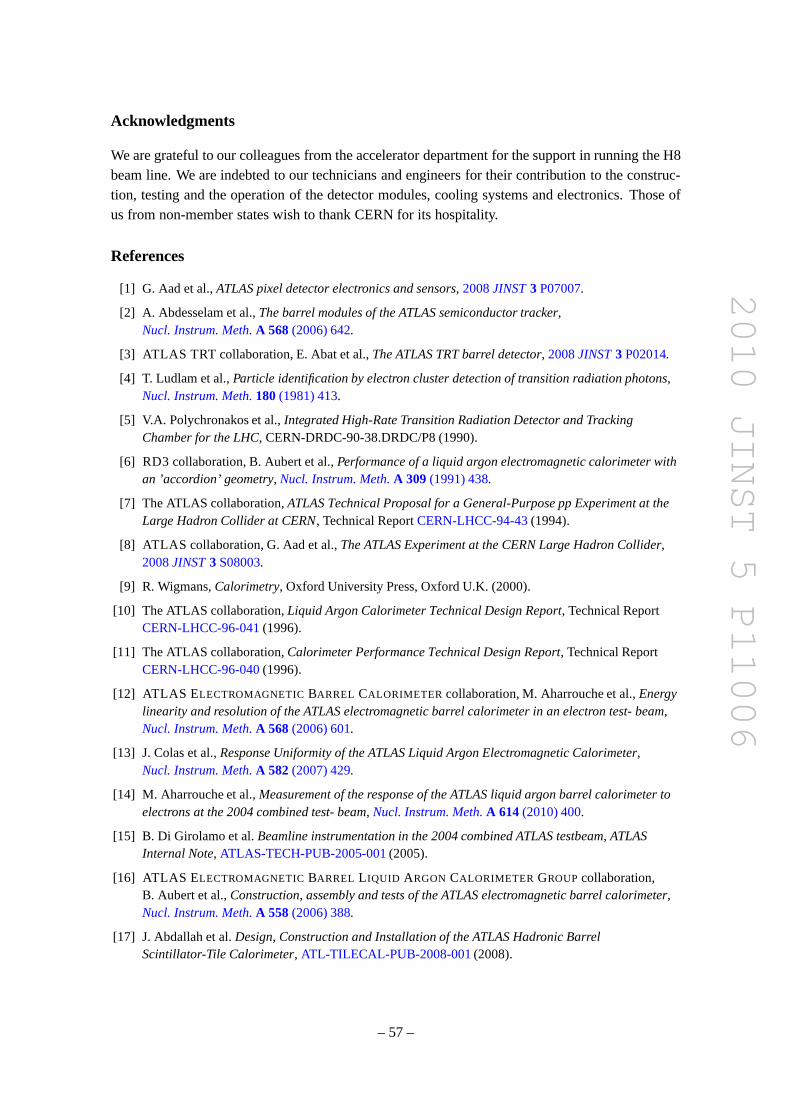
2010 JINST 5 P11006

Acknowledgments

We are grateful to our colleagues from the accelerator department for the support in running the H8beam line. We are indebted to our technicians and engineers for their contribution to the construc-tion, testing and the operation of the detector modules, cooling systems and electronics. Those ofus from non-member states wish to thank CERN for its hospitality.

References

[1] G. Aad et al.,ATLAS pixel detector electronics and sensors, 2008JINST3 P07007.

[2] A. Abdesselam et al.,The barrel modules of the ATLAS semiconductor tracker,Nucl. Instrum. Meth.A 568 (2006) 642.

[3] ATLAS TRT collaboration, E. Abat et al.,The ATLAS TRT barrel detector, 2008JINST3 P02014.

[4] T. Ludlam et al.,Particle identification by electron cluster detection of transition radiation photons,Nucl. Instrum. Meth.180(1981) 413.

[5] V.A. Polychronakos et al.,Integrated High-Rate Transition Radiation Detector and TrackingChamber for the LHC, CERN-DRDC-90-38.DRDC/P8 (1990).

[6] RD3 collaboration, B. Aubert et al.,Performance of a liquid argon electromagnetic calorimeterwithan ’accordion’ geometry, Nucl. Instrum. Meth.A 309 (1991) 438.

[7] The ATLAS collaboration,ATLAS Technical Proposal for a General-Purpose pp Experiment at theLarge Hadron Collider at CERN, Technical ReportCERN-LHCC-94-43(1994).

[8] ATLAS collaboration, G. Aad et al.,The ATLAS Experiment at the CERN Large Hadron Collider,2008JINST3 S08003.

[9] R. Wigmans,Calorimetry, Oxford University Press, Oxford U.K. (2000).

[10] The ATLAS collaboration,Liquid Argon Calorimeter Technical Design Report, Technical ReportCERN-LHCC-96-041(1996).

[11] The ATLAS collaboration,Calorimeter Performance Technical Design Report, Technical ReportCERN-LHCC-96-040(1996).

[12] ATLAS ELECTROMAGNETIC BARREL CALORIMETER collaboration, M. Aharrouche et al.,Energylinearity and resolution of the ATLAS electromagnetic barrel calorimeter in an electron test- beam,Nucl. Instrum. Meth.A 568 (2006) 601.

[13] J. Colas et al.,Response Uniformity of the ATLAS Liquid Argon Electromagnetic Calorimeter,Nucl. Instrum. Meth.A 582 (2007) 429.

[14] M. Aharrouche et al.,Measurement of the response of the ATLAS liquid argon barrelcalorimeter toelectrons at the 2004 combined test- beam, Nucl. Instrum. Meth.A 614 (2010) 400.

[15] B. Di Girolamo et al.Beamline instrumentation in the 2004 combined ATLAS testbeam, ATLASInternal Note, ATLAS-TECH-PUB-2005-001(2005).

[16] ATLAS ELECTROMAGNETIC BARREL L IQUID ARGON CALORIMETER GROUPcollaboration,B. Aubert et al.,Construction, assembly and tests of the ATLAS electromagnetic barrel calorimeter,Nucl. Instrum. Meth.A 558 (2006) 388.

[17] J. Abdallah et al.Design, Construction and Installation of the ATLAS Hadronic BarrelScintillator-Tile Calorimeter, ATL-TILECAL-PUB-2008-001(2008).

– 57 –

2010 JINST 5 P11006

[18] F. Bauer et al.,Large-scale production of monitored drift tube chambers for the ATLAS muonspectrometer, Nucl. Instrum. Meth.A 518 (2004) 69.

[19] A. Ahmad et al.,Alignment of the Pixel and SCT Modules for the 2004 ATLAS Combined Test Beam,2008JINST3 P09004.

[20] N.J. Buchanan et al.,ATLAS liquid argon calorimeter front end electronics, 2008JINST3 P09003.

[21] J. Colas et al.,Electronics calibration board for the ATLAS liquid argon calorimeters,Nucl. Instrum. Meth.A 593 (2008) 269.

[22] A. Artamonov et al.,The ATLAS forward calorimeters, 2008JINST3 P02010.

[23] L IQUID ARGON BACK END ELECTRONICScollaboration, A. Bazan et al.,ATLAS liquid argoncalorimeter back end electronics, 2007JINST2 P06002.

[24] M. Aleksa et al.,ATLAS Combined Testbeam: computation and validation of theelectroniccalibration constants for the electromagnetic calorimeter, ATLAS Internal Note,ATL-LARG-PUB-2006-003(2006).

[25] S. Gadomski et al.,Deployment and use of the ATLAS DAQ in the combined test beam,IEEE Trans. Nucl. Sci.53 (2006) 2156.

[26] The ATLAS collaboration,ATLAS Computing TDR, Technical ReportCERN-LHCC-2005-022(2005).

[27] W.E. Cleland and E.G. Stern,Signal processing considerations for liquid ionization calorimeter in ahigh rate environment, Nucl. Instrum. Meth.A 338 (1994) 467.

[28] D. Banfi, M. Delmastro and M. Fanti,Cell response equalisation of the ATLAS electromagneticcalorimeter without the direct knowledge of the ionisationsignals, 2006JINST1 P08001.

[29] L. Neukermans, P.Perrodo and R. Zitoun,Understanding the electromagnetic barrel pulse shapes andthe absolute electronic calibration, ATLAS Internal NoteATL-LARG-2001-008(2001).

[30] M. Citterio, M. Delmastro and M. Fanti,A study of the electrical properties and of the signal shapesin the ATLAS Liquid ARgon Accordion Calorimeter using a hardware model, ATLAS Internal NoteATL-LARG-2001-018(2001).

[31] D. Prieur,Using Time Convolution Method to compute Optimal FilteringCoefficients for LARGelectromagnetic calorimeter, ATLAS Internal NoteATL-LARG-2005-001(2005).

[32] W. Lampl et al.Calorimeter Clustering Algorithms: Description and Performance, Technical ReportATL-LARG-PUB-2008-002, ATL-COM-LARG-2008-003 (2008).

[33] GEANT4 collaboration, S. Agostinelli et al.,GEANT4: a simulation toolkit,Nucl. Instrum. Meth.A 506 (2003) 250.

[34] B. Di Girolamo, M. Gallas and T. Koffas,2004 ATLAS Barrel Combined Test Beam Layout, ATLASEDMS Note, ATC-TT-IN-0001 (2005).

[35] F. Hubaut, B. Laforge, D. Lacour, F. Orsini,Test beam Measurement of the Cross-talk in the EMBarrel Module 0, ATLAS Internal NoteATL-LARG-2000-007(2000).

[36] F. Hubaut,Crosstalk Measurements in the EM Barrel Module 0 from 99’, May 00’ and July 00’ BeamTests, ATLAS Internal NoteATL-LARG-2000-009(2000).

[37] M. Boonekamp, Private communication.

[38] M. Delmastro, M. Aleksa, T. Carli, R. Froeschl, I. Wingerter-Seez,Response of the ATLAS LiquidArgon Electromagnetic Barrel Calorimeter to Very Low Energy Electrons at the 2004 ATLASCombined Test-Beam, ATLAS Internal Note ATL-COM-LARG-2009-014 (2009).

– 58 –

2010 JINST 5 P11006

[39] W. Lampl,Optimizing the Energy Measurement of the ATLAS Electromagnetic Calorimeter, PhDthesis, Vienna University of Technology (2006)CERN-THESIS-2006-002, Presented on 18 Jan 2006

[40] D. Banfi, L. Carminati and L. Mandelli,Calibration of the ATLAS electromagnetic calorimeter usingcalibration hits, ATLAS NoteATL-LARG-PUB-2007-012(2007).

[41] T.G. Cornelissen et al.,Track Fitting in the ATLAS Experiment, PhD thesis, Univ. Amsterdam (2006)CERN-THESIS-2006-072, Presented on 12 Dec 2006.

[42] T. Koffas and T. Vu Anh, Private communication.

[43] A Wald and J Wolfowitz,On a test whether two samples are from the same population,Ann. Math Statist.11 (1940) 147.

[44] V Kartvelishvili, Electron bremstrahlung recovery in ATLAS tracking using Dynamic NoiseAdjustment, PoS(ACAT)046.

[45] T Atkinson,Reconstruction of electrons with the Gaussian-Sum filter inthe ATLAS Inner Detector,52nd IEEE Nuclear Science Symposium and Medical Imaging Conference, pages 148–152 (2005).

[46] M. Aleksa et al.,Measurement of the ATLAS solenoid magnetic field, 2008JINST3 P04003.

[47] R. Froeschl,Calibrating the CERN ATLAS Experiment with E/p, CERN-THESIS-2010-007PhDthesis, Vienna Tech. University (2009), Presented on 14 Oct2009.

[48] J.E. Gaiser,Charmonium Spectroscopy from Radiative Decays of the J/ψ andψ ′, PhD thesis,SLAC-R-255 (1982), the Crystal Ball function is defined in appendix F, p.178.

– 59 –