combined supplemental skh feb 18 2016 - afán por saber · abundant carbonate nodules, calcified...
TRANSCRIPT

SECTION 1. GEOLOGICAL AND DEPOSITIONAL SETTING
The Cerutti Mastodon (CM) bonebed (Bed E) and strata preserving other invertebrate and
vertebrate fossil remains were contained within a 12 m-thick series of flat-lying, late Pleistocene
fluvial sediments that unconformably overlie the upper Oligocene Otay Formation and upper
Pliocene San Diego Formation above an irregular erosion surface1. Although not exposed at the
surface, the Otay Formation and San Diego Formation in this area are in fault contact along a
north-south fault splay of La Nacion Fault Zone2. There is no evidence that the Pleistocene
deposits are offset by this faulting. Overall, the Pleistocene sediments consist of cyclic sequences
of fining-upward sedimentation units, grading from conglomeratic sands to silts. The most
common lithologies are reddish-brown, fine-grained, micaceous, compact, silty sands and brown,
poorly sorted, somewhat compact silts. Some of the silt beds contain large amounts of soil
carbonate (caliche), as well as ped structures, suggesting development as paleosols in an
overbank depositional setting. In addition, the conglomeratic sands are often cross-stratified,
suggesting deposition in active stream channels. Together, these sedimentological conditions
suggest deposition in a meandering river near base level.
Pleistocene sediments are widespread in the coastal region of San Diego County,
although in most cases these sediments are associated with elevated marine abrasion platforms
(terraces) that formed during periods of marine high stillstands on a rising coastline. Earlier
studies have summarized the age and distribution of these abrasion platforms and their associated
sedimentary covers and provided a terrace chronology for the coastal region3, 4. By far the most
extensive Pleistocene marine terrace is the Nestor Terrace, which has been radiometrically dated
at 120 ka and correlated with MIS 5e3, 5. The shoreline angle for the Nestor abrasion platform
averages 22-23 m above mean sea level (amsl) and serves as a proxy for the relative position of
WWW.NATURE.COM/NATURE | 1
SUPPLEMENTARY INFORMATIONdoi:10.1038/nature22065

sea level in this area during MIS 5e. Largely because of faulting associated with La Nacion Fault
Zone and the Rose Canyon Fault Zone to the west2, there are no exposures of the marine Nestor
Terrace in the immediate vicinity of the CM site. Consequently, it is not possible to directly
correlate the Pleistocene CM and Nestor Terrace stratigraphic sequences by reconstructing paleo
stream gradients. It is noteworthy, however, that the Nestor Terrace shoreline angle is below the
elevation of the CM bonebed (~45 m amsl), which lies approximately 6 km inland from the
eastern shore of present day San Diego Bay. The resulting minimum elevation difference
between the CM site and the Nestor Terrace shoreline angle is 23 m, which suggests a gradient
of ~3.8 m per km compared to ~2.1 m per km for the modern Sweetwater River in its lower
reaches. This difference in gradient suggests that the Pleistocene surface at the CM site is older
than the Nestor Terrace (i.e., older than 120 ka).
The microstratigraphy at the CM site consists of four primary horizons, including in
ascending order: Bed C (a 105 cm-thick, rusty brown, massive, micaceous silt), Bed D (a 21 cm-
thick, yellowish, fine- to coarse-grained, massive to cross-bedded, friable, arkosic sand with
heavy mineral laminations), Bed E (a 20-30 cm-thick, medium brown, massive, sandy silt with
abundant carbonate nodules, calcified root casts and pyrolusite staining) and Bed F (a 20 cm-
thick, rusty brown, massive, clayey silt with common small carbonate nodules).
With the exception of some shells of pulmonate gastropods and rodent teeth from Beds D
and F, the vast majority of fossils recovered from the CM site were recovered from Bed E and
consist of mineralized bones, bone fragments and teeth of a single individual of Mammut
americanum. Other fossils collected from Bed E include remains of rodents, birds, reptiles and
terrestrial invertebrates. There was no articulation of mastodon skeletal elements and no
anatomical trend to their position in the bonebed. Many bones are fragmentary and display
WWW.NATURE.COM/NATURE | 2
SUPPLEMENTARY INFORMATIONRESEARCHdoi:10.1038/nature22065

distinct types of breakage. In one case, refitting pieces of a single mastodon molar were found
spread over three different grid units (Fig. 1c). The anterior half of the tooth (CM-286) was
found in grid unit E3, while the posterior half (CM-103) came from grid unit C1. An enamel
cusp fragment (CM-148) of this same tooth was found in grid unit D2. The greatest
concentration of bones came from grid units D3 and E3, which contained portions of molars,
long bones, and ribs (Concentration 1; Fig. 1). Of special note was the discovery of both femur
heads side-by-side, one (CM-252) with its articular surface up and one (CM-258) with its
articular surface down (Extended Data Fig. 3b). Adjacent to the femur heads lay fragments of
ribs, one of which (CM-253) was found lying directly on a pegmatite cobble fragment (CM-254).
Also found in this concentration was a large piece of femoral diaphysis displaying distinct spiral
fracturing and evidence of percussion (CM-288; Fig. 1c; Extended Data Fig. 4a-e;
Supplementary Video 3). In grid units J4 and K4 a large, spirally-fractured piece of long bone
(CM-340) was found with a distinct impact notch (Fig. 2d; Supplementary Video 4). This
fractured bone occurs adjacent to two complete thoracic vertebrae and two complete ribs (Fig.
1a). In grid unit B2 the distal 70 cm of a tusk (CM-56) was found distal end down in an upright
orientation (62°-64° dip), concave curvature to the south. The proximal end of the tusk had been
removed by the backhoe at the level of Bed E (shown as a circular feature in grid unit B2; Fig.
1a; Extended Data Fig. 3c). The tusk extended from Bed E through Bed D, reaching 65 cm into
Bed C (Extended Data Fig. 7c). Coarse-grained sand matrix from Bed D was found as an
infilling alongside the tusk some 40 cm into Bed C.
In contrast to the disarticulated condition of the mastodon remains was the discovery of a
partially articulated skeleton of Fulica americana (American Coot) collected in grid unit B5. The
entire pectoral region, including the right and left wings and coracoids, was found still articulated
WWW.NATURE.COM/NATURE | 3
SUPPLEMENTARY INFORMATIONRESEARCHdoi:10.1038/nature22065

with the sternum. Articulated portions of the legs were also recovered. In addition, several rodent
skulls recovered from Bed E were found with articulated lower jaws.
The large cobbles and smaller cobble fragments recovered from Bed E (Fig. 1a; Extended
Data Fig. 3e, f) consist of fine-grained metavolcanic cobbles (andesite) and coarse-grained
plutonic cobbles (pegmatite). These lithic clasts range from approximately 1 to 30 cm in
diameter. The more intact, larger cobbles display smoothly rounded surfaces, while many of the
smaller cobble fragments have sharp, angular edges that lack signs of abrasion. Of the larger
cobbles (>20 cm), four are andesites (CM-7, 114, 281 and 383) and one is a pegmatite (CM-423)
(Fig. 4a, e, f; Extended Data Fig. 5g, h). There are several instances in which cobble fragments
and/or large cobbles found separated in the bonebed could be refitted after laboratory preparation
(removal of caliche). In the case of the large cobble (CM-423) found in grid unit G5, six cobble
fragments in grid units D3, E2 and E3 were refitted to it (Supplementary Video 7). The grid unit
E2 cobble fragment (CM-109) was separated by over 3 m of bonebed from the parent cobble
(CM-423) in grid unit G5. Several other small fractured pegmatite cobble fragments were also
found in Concentration 1 that could not be refitted to the large cobble. However, it is plausible
that all these pegmatite cobble fragments are part of the same original cobble.
Approximately 7,300 kg of Bed E matrix was stockpiled and screenwashed. The washed
concentrate produced isolated dental remains of small mammals including rodents (e.g.,
Microtus, Neotoma, Peromyscus and Thomomys) and rabbit (Sylvilagus). Calcareous
nodules/internal shells of a slug (Deoroceras), were also recovered from the washed concentrate.
SECTION 2. SEDIMENT ANALYSIS
Soil stratigraphic, pipette grain-size, thin section and x-ray diffraction analyses (Extended
Data Fig.1b, c) of the CM bonebed (Bed E) and the beds immediately above and below (Beds F
WWW.NATURE.COM/NATURE | 4
SUPPLEMENTARY INFORMATIONRESEARCHdoi:10.1038/nature22065

and D, respectively) suggest low-energy fluvial deposition followed by pedogenesis. Soil and
sediment descriptions reveal a well-developed Bt-Bk-C profile (Beds F, E and D respectively)
with moderate to strong, very coarse, angular to subangular blocky structures in the Bt and Bk
horizons (Extended Data Fig.1b, c; Supplementary Table 1). Clay films on ped faces and
pedogenic carbonates are present. Further evidence for pedogenesis is provided by root etching
on mastodon bones and rhizohalos in the Bk horizon6. Total sand from sediment size-analysis
reveals a clear upward-fining sequence through the Bt-Bk-C profile (Extended Data Fig. 1c).
These data, coupled with the presence of cross-bedding in the C horizon in Bed D (Extended
Data Fig. 1b) indicate fluvial deposition. Total clays increase near the top of the Bt and Bk
horizons and decrease with depth through each horizon (Extended Data Fig. 1c), another typical
pedogenic signature. X-ray diffraction of the clay minerals in Bed E suggests that they are
dominated by smectite, an indicator of soil development. Thin section analysis of sediments in
Bed E reveals subangular granitic mineral grains; these also are dominant in the fluvial cross-
bedded sands of Bed D. This suggests that beds D and E have the same lithologic source and is
strong evidence that both beds were stream-deposited.
WWW.NATURE.COM/NATURE | 5
SUPPLEMENTARY INFORMATIONRESEARCHdoi:10.1038/nature22065

Supplementary Table 1. Soil and sediment descriptions. Color: refers to comparison with Munsell soil color chart value. Structure: 1-weak, 2-moderate, 3-strong, f-fine, m-medium, vc-very coarse, abk-angular blocky, sbk-sub angular blocky. Consistence: Wet; so-nonsticky, s-sticky, vs-very sticky, po-nonplastic, vp-very plastic. Dry; so-soft, h-hard. Pores: 1-few, 2-common, vf-very fine, f-fine, m-medium. Texture: LS-loamy sand, SiC-silty clay. Clay films: 1-few, f-faint, d-distinct, pf-ped faces. Stage: refers to the amount of soil-carbonate accumulation based on four-stages from low (I) to high (IV).
Layer Horizon Color Structure Gravel
%
Consistence Pores Texture
Clay films
Stage Notes Wet Dry
Bed-F Bt 10 YR 6/4 (dry) 10 YR 4/3 (wet)
2/3, vc, abk/sbk 0 s/vs, vp h 1m, 2f/vf
SiC 1, f, pf
I+ none
Bed-E Bk 10 YR 6/2 (dry) 10 YR 5/3 (wet)
2/3, vc, abk/sbk 0 s/vs, vp h 1m/f,
2vf SiC
1, f/d, pf
II+ mastodon layer,
root etching on bones
Bed-D C 1, f/m, sbk 0 so, po so 1m, 1vf
LS none trough cross-bedding
WWW.NATURE.COM/NATURE | 6
doi:10.1038/nature22065 SUPPLEMENTARY INFORMATIONRESEARCH

In summary, the depositional environment for Beds D, E and F represents a slowly
aggrading fluvial system. A flood plain depositional setting is strongly supported by sediment
particle-size data. Post-mortem, the mastodon bones and associated cobbles eventually were
buried by continued low-energy fluvial deposition. The pedogenic A horizon, which likely
formed on a paleo-landscape above the mastodon bonebed, has been removed by erosion. As the
Bt and Bk horizons developed, pedogenic clays and calcium carbonate accumulated, and some of
the bones and cobbles became encased in calcium carbonate. This pedogenic evidence indicates
that although erosion removed the A horizon developed at the top of Bed E, the preserved
portion of Bed E consisting of the developed Bt and Bk horizons is undisturbed by later fluvial
or other geologic processes.
Alternative explanations for the formation of the bonebed, for example high-energy flood
deposits and plunge pools formed during high-flow conditions, can be rejected for several
reasons. High-flow conditions would have size-sorted the bone and cobble fragments with less
dense fragments being deposited far downstream. Two sets of mammoth remains have been
recently excavated from plunge pool deposits in the central United States. At the first site7, the
mammoth died on a point bar and desiccated to the point that the skull fragmented, the molars
became isolated and the tusk disintegrated into fragments. A subsequent flood event redeposited
generally oblong elements over the end of the point bar into a small plunge pool. Here molars, a
phalanx and several tusk fragments were found in a jumbled accumulation. Subsequently,
complete limb elements were found on the point bar deposit upstream. The second site was in an
alluvial fan setting (report in progress). Less dense elements like rib fragments, vertebrae and the
brain case were distributed down a narrow paleo-gully and deposited in a pile in a plunge pool
with elements lying at high angles of repose. At both these sites, size and density similarities
WWW.NATURE.COM/NATURE | 7
SUPPLEMENTARY INFORMATIONRESEARCHdoi:10.1038/nature22065

determined which elements were differentially moved in relatively high-energy fluvial events.
These conditions are quite dissimilar to the CM site where elements of all sizes and density,
including large cobbles and tiny bone fragments, were found distributed in a 20-30 cm-thick
deposit of silts and fine sands with no evidence of disturbance by high-energy fluvial events.
The lack of evidence of high-energy fluvial conditions at the CM site also calls into
question possible alternative explanations for the occurrence of tusk CM-56, which was found
vertically oriented and extending from Bed E down into the underlying strata through Bed D into
Bed C. What strictly fluvial conditions could be responsible for orienting one tusk (CM-57)
horizontally and the other (CM-56) vertically? And besides human activity, what purely
biological conditions could be responsible for this taphonomic pattern? It appears to be
impossible that a mastodon could somehow force its own tusk into the underlying deposits,
because the mastodon would have to have been positioned completely vertical to drive its tusk
into the deposits at the required angle (Extended Data Fig. 7c). With geological and biological
processes eliminated, the most reasonable hypothesis for the vertical orientation of the tusk is
that the tusk came out of the skull naturally, or possibly was removed from the skull by humans,
and that the tusk was then purposely socketed by humans deep into the underlying deposits for
some unknown reason.
SECTION 3. USEWEAR AND IMPACT MARKS ON CM HAMMERSTONES AND ANVILS
CM-7, Andesite Cobble.
This cobble measures 27.4 cm-long, 15.6 cm-wide and 15.7 cm-thick and weighs 8.85 kg
(Extended Data Fig. 5j). The cobble was found on the eastern margin of Concentration 2 (Fig.
1a). One corner of the cobble was hit by the backhoe when the site was first discovered and has a
small amount of damage along one edge over a distance of 95 mm. This modern damage is easily
WWW.NATURE.COM/NATURE | 8
SUPPLEMENTARY INFORMATIONRESEARCHdoi:10.1038/nature22065
recognized by the fresh coloration of the fracture. An unknown, but significant, part of the
cobble is missing as indicated by a fracture plane forming a flat edge that occurred prior to the
time of burial when the CM site formed and before excavation. A flake (CM-141) that refits to
the broken surface (Extended Data Fig. 5m) was found in situ two meters from CM-7. Numerous
sharp andesite fragments were also found in the general area and although they do not refit to the
cobble, they may have come from the missing part of the cobble. Cobble CM-7 is hypothesized
to have been used as a hammerstone based on the presence of usewear and impact damage, its
position away from the main concentrations of fractured bone and molars, the breakage pattern
and the refitting flake that was found one meter from andesite cobble anvil CM-114 (Fig. 3).
Usewear on the upper surface of CM-7 includes relatively fresh fractures (step scars, undetached
flakes) and impact features (Hertzian initiations) along two battered margins suggesting that CM-
7 may also have functioned as an anvil. Several phases of wear formation are indicated by
variation in the intensity of edge rounding (Extended Data Fig. 5l). The intensity of edge
rounding is higher on the external platform edge of flake CM-141 than on the internal platform
edge, which is relatively fresh. The edge rounding is also higher on the external platform edge of
flake CM-141 than on the battered margins of CM-7.
CM-114, Andesite Cobble.
This cobble measures 19.9 cm-long, 16.2 cm-wide and 11.3 cm-thick and weighs 4.15
kg. The cobble was found at the center of Concentration 2, which contained impact-fractured
bone and molar fragments and broken andesite fragments (Fig. 1b). The upper surface exhibits
breakage, including fresh fracture surfaces with thin pieces of the cobble cortex missing. The
breakage appears to occur along a pre-existing natural fracture plane and is hypothesized to be
damage from impact. The underside of the cobble is relatively flat, which would have provided a
WWW.NATURE.COM/NATURE | 9
SUPPLEMENTARY INFORMATIONRESEARCHdoi:10.1038/nature22065
solid base for its use as an anvil. There is a flake scar present on this under surface, although the
flake was removed before the cobble was introduced to the site, as indicated by the rounded
edges of the flake scar. However, along the proximal edge of the old flake scar (which forms a
relatively low edge angle with the upper cobble surface), there are fresher fractures and impact
scars, including undetached flakes. The latter are similar to fresh scars on the upper surface ridge
and indicate stone-on-stone impact. The weathered upper cortical surface also has small zones
with striations and abrasive polish consistent with impact on bone and stone. CM-114 is
interpreted as an anvil based on its location at the center of this concentration, its relatively small
size (probably too small to be an effective hammerstone) and usewear on the top of the cobble.
CM-383, Andesite Cobble.
This round flat cobble measures 23.7 cm-long, 22.5 cm-wide and 10.7 cm-thick and
weighs 7.6 kg (Fig.4e, f; Extended Data Fig. 3e). The cobble was found approximately 2 m
southwest of Concentration 1 in grid unit H4 (Fig. 1a). The cobble exhibits macro- and
microscopic wear on the surface that was found lying upward, with the under surface exhibiting
a rougher surface texture. There is an impact flake removed from one edge on the under surface
(Fig. 4h). The flake scar appears fresh and occurs on an older broken surface that exhibits
extensive rounding. The flake removed the weathered light tan surface of the cobble. The flake
scar exhibits an impact point, radiating lines of force and a feathered termination. The flake scar
is 24.2 mm-wide at the point of initiation, expands to a maximum width of 28.2 mm and is 25
mm-long. A small ovoid flake scar that terminates in a hinge fracture occurs within the larger
flake scar. This secondary flake scar is 8.9 mm-long, 13.5 mm-wide at the point of initiation and
8.9 mm-long. There is an area of impact damage to one side of the flake scar. This area exhibits
an incipient flake crack. The cobble experienced at least two blows in this area. CM-383 is
WWW.NATURE.COM/NATURE | 10
SUPPLEMENTARY INFORMATIONRESEARCHdoi:10.1038/nature22065
hypothesized to have been used as a hammerstone, although it could also have served as an anvil
based on the use wear present on the upper face of the cobble.
CM-281, Andesite Cobble.
This long, thick, domed cobble measures 29 cm-long, 18.6-cm wide and 14.7 cm-thick
and weighs 8.3 kg (Fig. 4a). This cobble was found at the center of Concentration 1 with impact-
fractured limb bones including three impact flakes, one impacted femur segment, one impact-
broken molar fragment, broken pegmatite fragments from a hammerstone, and other broken
fragments of bone, molars and andesite (Fig. 1b). The cobble exhibits macroscopic and
microscopic wear along a 103 mm-long ridge on the upper surface. Oriented in line with
striations and, along this upper edge, are small flake scars with step terminations indicating
stone-on-stone impact (Fig. 4b-d). Based on its location at the center of Concentration1 and
usewear, CM-281 is interpreted as an anvil.
CM-423, Pegmatite Cobble.
This is the largest cobble discovered at the site, measuring 29.8 cm-long, 26.4 cm-wide
and 13.8 cm-thick and weighing 14.45 kg (Extended Data Figs 3f and 5g). The cobble is even
larger when six refit pieces (CM-109, 254, 262, 283, 284 and 304) are included (Fig. 3;
Supplementary Video 7). With the refitting pieces the cobble weighs 18.25 kg. The cobble was
found approximately 2 m southwest of Concentration 1 in grid unit G5 (Fig. 1a). Five of the six
refitting pieces were found within 0.5 m of andesite anvil CM-281 in the center of Concentration
1 (Fig. 3). Two other small fragments of fractured pegmatite that were probably part of this
hammerstone were also found, but have not been refitted to CM-423. This pegmatite cobble
exhibits very coarse crystalline structure including large feldspar phenocrysts which cause
natural fracture (cleavage) planes in the cobble (see description of CM-254). Percussion impact
WWW.NATURE.COM/NATURE | 11
SUPPLEMENTARY INFORMATIONRESEARCHdoi:10.1038/nature22065

is indicated by deep cracks and macroscopic pitting at one end, where the cortical surface has
been removed (Extended Data Fig. 5h). CM-423 is interpreted to be a hammerstone based on its
size, breakage patterns, refits with other fragments found associated with the anvil and
surrounding impact-fractured mastodon limb bone and evidence of impact.
CM-254, Pegmatite Cobble.
This is the largest pegmatite fragment that refits onto cobble CM-423, measuring 17.6
cm-long, 12.4 cm-wide and 8 cm-thick and weighs 2.15 kg. The cobble was found in
Concentration 1 with fractured bone, broken andesite and pegmatite fragments and broken molar
fragments adjacent to andesite cobble anvil CM-281 (Fig. 3). CM-254 was found with the outer
surface down and the broken surface upward and in direct contact with an overlying broken rib
(CM-253). A broken bone (CM-263) was found lying beneath CM-254, and can be refitted with
CM-255. There are large feldspar phenocrysts at both broken ends of this cobble that broke along
cleavage planes, probably when the tip of the hammerstone separated from the main body of
CM-423 during a percussion event. CM-254 has rare patches of abrasive smoothing with fine
striations but no clear examples of impact (e.g., pitting caused by hammer blows) that are
typically, but not always found on stone pounding implements used to break bones. CM-254 is
interpreted to be the tip of a hammerstone based usewear, breakage patterns, refits with other
fragments found associated with the anvil and with the large cobble CM-423, and its association
with impact-fractured mastodon limb bone around the anvil.
Andesite Cobble Fragments, CM-1, 49, 53, 87, 93c, 228 and 431.
These seven andesite fragments were found in Concentration 2 (Fig. 3), and although
they all can be refitted together, they do not refit with any recovered larger cobbles and may
indicate the presence of a sixth cobble based on their very smooth outer surfaces which do not
WWW.NATURE.COM/NATURE | 12
SUPPLEMENTARY INFORMATIONRESEARCHdoi:10.1038/nature22065

match surfaces on the other andesite cobbles. There is also a possibility that these reassembled
andesite fragments are part of the missing portion of hammerstone CM-7 and just have smoother
outer surfaces than those preserved on CM-7.
SECTION 4. PROBOSCIDEAN TAPHONOMY – NATURAL VERSUS CULTURAL MODIFICATION OF
LIMB BONES
Taphonomy of the CM bonebed is best explained within the broader context of the
mechanics of bone breakage. Once the mechanics of bone breakage are defined, it is then
possible to determine whether natural or anthropogenic processes modified CM proboscidean
limb bones. Natural processes that can modify proboscidean limb bones include environmental,
geologic and non-cultural biologic factors, including carnivore activity, trampling by other
animals and rodent gnawing. Human use of proboscidean limb bone typically is characterized by
a percussion technology used to break limb bones for marrow extraction and tool production8.
Mechanics of Proboscidean Limb Bone Breakage
Comprehensive reviews of the mechanical principles of bone taphonomy have been
published8, 9 and provide a rigorous context for exploring the modifications present, or
significantly absent, on bone from the CM site.
Three categories of bone fracturing processes have been described, including passive
fracturing, static fracturing and dynamic fracturing8. Passive fracturing occurs when weathering,
which causes desiccation (drying) and chemical decomposition of bone, induces microscopic
cracks between the collagen bundles in the bone structure8. Because the time required for total
bone destruction by weathering can vary depending on the skeletal element involved (e.g., femur
vs. rib) and on multiple environmental factors (e.g., temperature, humidity or seasonality), it has
been possible to establish a graded series of bone weathering stages10. Weathered bone does not
WWW.NATURE.COM/NATURE | 13
SUPPLEMENTARY INFORMATIONRESEARCHdoi:10.1038/nature22065
retain the viscoelastic and ductile properties of fresh (green) bone. Characteristic modifications
of weathered long bones include a series of perpendicular, diagonal or right angle offset fractures
caused by tension failure, especially when the bone is later subjected to external forces such as
dynamic or static fracturing processes.
Static fracturing is caused by applying constant compressive forces that are evenly
distributed8 such as those produced by carnivoran bite forces or sediment loading. Dynamic
fracturing is caused by high velocity impacts that produce compression, twisting and shearing
forces8. The characteristics of fractures produced by static and dynamic fracturing processes
depend on whether the bone is desiccated or fresh. Desiccated bone exhibits dry-bone fracture
patterns that include longitudinal or perpendicular fracture planes with rough surfaces. Bones
with spiral fractures8 and fracture planes with smooth surfaces11 indicate the bone was broken
while fresh (green), but do not conclusively identify the agent that caused the fracture8, 9.
Dynamic fracturing of fresh bone is, however, a characteristic of hominin action because
percussion technology is used to modify bones for nutritional or manufacturing purposes.
Certain bone surface features are also indicative of dynamic fracturing of fresh bone
because they indicate a viscoelastic response to tensile and compressive forces. Characteristic
features include hackle marks, which are stress relief fractures concave to the origin of impact,
step terminations that indicate interruptions in the propagation of force and cone flakes and
negative impact scars that are a response to compressive force8.
Weathering
Evidence indicating weathering of bone at the CM site is variable. The majority of limb
bones do not exhibit extensive weathering cracks (i.e., weathering stage 0 or 110), while ribs and
vertebrae exhibit some cracks that represent wetting and drying processes and/or diagenetic
WWW.NATURE.COM/NATURE | 14
SUPPLEMENTARY INFORMATIONRESEARCHdoi:10.1038/nature22065

processes related to formation of pedogenic carbonate (caliche). All weathering-like features
appear to post-date the disarticulation and burial of CM bones. In addition, some limb element
fragments e.g., CM-288) with unweathered surfaces are spirally-fractured, with smooth
curvilinear fracture planes indicating that the bone was broken while it was still fresh (Extended
Data Fig. 4a-e; Supplementary Video 3). Some CM elements (e.g., CM-340) preserved within
carbonate concretions exhibit dry-bone breakage that is attributed to post-depositional diagenesis
during or after pedogenic carbonate deposition (Supplementary Video 4).
Geologic Processes of Proboscidean Limb Bone Modification
Two geologic processes that might modify proboscidean limb bones at the CM site were
considered; fluvial transport and sediment loading. Soil analysis (Supplementary Information
section 2), as well as the presence of very small bone fragments and a fragile semi-articulated
skeleton of an American coot (SDNHM 51967, 20 associated elements) within the CM bonebed
attest to a low-energy overbank deposition of silt and fine sand. This low-energy depositional
regime indicates transport by water was not a factor in moving the bones and cobbles or causing
the observed breakage patterns.
The weight of overlying sediments (sediment loading) can sometimes break light bones
after they have dessicated9. However, dry bone breakage patterns are easy to recognize and the
resulting dry-fractured fragments typically lie close together. There is no evidence of sediment
loading on the CM mastodon bones. However, there is dry-bone fracturing evident on some
elements that were encased in pedogenic carbonate concretions, apparently the result of wetting
and drying cycles and/or diagenesis during formation of the concretions. Post-depositional dry-
bone fracturing, as evidenced by longitudinal and perpendicular fracture planes with rough
surfaces is distinguished from the spiral fracture patterns produced by dynamic fracturing of
WWW.NATURE.COM/NATURE | 15
SUPPLEMENTARY INFORMATIONRESEARCHdoi:10.1038/nature22065

16
fresh bone noted on the majority of CM limb bone fragments. There is no evidence at the CM
site that geological processes caused breakage of fresh mastodon limb bones.
Biologic Processes of Proboscidean Limb Bone Modification
Two biologic processes, carnivoran gnawing and trampling by large mammals, are
known to fracture bone9. However, fresh cortical proboscidean limb bone is rarely broken by
either agent12.
Carnivoran gnawing is a common phenomenon in the paleontological record9. Bone
modification by large carnivorans is limited by jaw size and muscle strength, nutritional content
of the bone and access to alternative foods. Carnivorans extract nutrients from bone by gnawing
first at the articular ends of the limb bone where the cortex is thin and then proceeding into the
diaphysis of the bone. Carnivorans cannot break adult or near-adult proboscidean limb bones at
mid-shaft8, 13.
This view is supported by observations at numerous excavated proboscidean sites14, 15, 16,
17, 18, and examination of proboscidean remains in museums in Canada, Mexico, and the USA.
No evidence for breakage of adult or near-adult proboscidean limb bones at mid-shaft by
carnivorans has been identified. Occasionally carnivoran gnawing has been observed on the
articular ends of proboscidean limb bones in the form of gouges and tooth drag marks19, like
those described below.
A taphonomic study of heavily gnawed elephant bones (Paleoloxodon antiquus) from
late Pleistocene deposits in Germany concluded that the bones were modified by hyenas
(Crocuta crocuta spelaea) and cave lions (Panthera leo spelaea), the largest late Pleistocene
bone-processing specialists in the European carnivoran guild19. Hyenas were the predominant
scavenger accounting for 95% of the damage on bone, which primarily consisted of tooth gouge
WWW.NATURE.COM/NATURE | 16
SUPPLEMENTARY INFORMATIONRESEARCHdoi:10.1038/nature22065

17
marks, gnawed epiphyseal ends of adult long bones and preferential preservation of cylindrical
long bone diaphyses too thick for the carnivorans to break. That study provides convincing
evidence that even the most specialized bone-modifying Pleistocene carnivorans could not break
adult or near-adult proboscidean limb bones at mid-shaft. The fact that no tooth gouge marks, no
gnawed epiphyseal ends and no cylindrical remnants of long bones were found at the CM site
suggests that carnivoran bone modification was not responsible for the observed breakage
patterns16, 20.
Trampling of proboscidean bones by large mammals is most common around watering
holes where drought or disease has caused mass die offs21. However, mass death sites around
watering holes where trampling by other elephants has occurred are not an appropriate analogy
for single death sites. One study22 has documented in detail bone scatters at seven sites involving
single modern elephant deaths and recorded only two fractured limb bones at the seven sites and
interpreted those fractures to be the result of the elephants thrashing around as they died. That
study concluded that “The paucity of such fractured limb bones in scatters suggests that not
much trampling or natural fracturing of weathered bone has occurred on the sites” 22.
Another study discussed single-elephant death sites both around watering holes and away from
watering holes23. Evidence of trampling was found less frequently at single elephant death sites
than at mass death sites around watering holes. The study concluded that bone scatters away
from water sources are rarely affected by trampling and kicking, that even single death sites at
water sources may not exhibit heavy trampling and that, “kicking and trampling are hit and miss
processes, unless elephants return in large number to the site seasonally, in which case bones
may be widely scattered and broken” 23.
WWW.NATURE.COM/NATURE | 17
SUPPLEMENTARY INFORMATIONRESEARCHdoi:10.1038/nature22065

18
Fracturing of proboscidean limb bones while still fresh is rare in modern single-elephant
death sites, and no sites have been documented like the CM site, where fresh elephant limb bone
is broken into numerous small spirally fractured fragments with evidence of multiple impacts.
The femoral diaphyses found at the CM site are broken into small spirally-fractured pieces,
whereas more fragile bones like ribs and vertebrae are complete, or more complete than the
heavier and denser limb bones. This pattern of differential breakage is exactly the opposite of
what is found where proboscidean bones have been extensively trampled. Under trampling, the
lightest bones (e.g., ribs and vertebrae) are broken first and into much smaller pieces than the
limb bones that have thicker cortical walls resistant to breakage23.
A recent study of trampled bones from several animals of different body sizes, including
elephants, found that trampling did not result in the production of impact notches like the one
found on the CM limb bones24. More experimental research is needed with larger samples to
further understand the possible features of trampling damage to fresh proboscidean limb bones at
single death sites. However, the typical surface features of bone modified by trampling25 (i.e.,
randomly distributed surface abrasions/striations that intersect and overlap) are not found at the
CM site. In particular, the specimens that show evidence of spiral fracture or impact show no
evidence of trampling. We conclude that trampling was not responsible for the breakage of the
CM limb bones.
Cultural Processes of Proboscidean Limb Bone Modification
Human use of proboscidean limb bone can best be understood within the framework of
the technological process used to break bones for marrow extraction and/or tool production.
Cultural processes that modify proboscidean limb bones and other bones have been studied for
more than 60 years in Europe26, 45 years in Africa27 and 35 years in North America12. Breakage
WWW.NATURE.COM/NATURE | 18
SUPPLEMENTARY INFORMATIONRESEARCHdoi:10.1038/nature22065
19
of proboscidean limb bone fits within a broader pattern of percussion technology used to break
limb bones of large ungulates for marrow extraction that dates to 2.5 Ma at the Bouri Site in
Ethiopia, Africa28. Proboscidean limb bone modification using percussion technology by early
members of the genus Homo began in Africa during the early Pleistocene27, 29, 30. Fractured and
flaked proboscidean limb bone, including one biface, has been reported from Olduvai in
Tanzania in deposits dating to 1.2 to 1.7 Ma27, 29, 30. One bone biface from the Konzo Site in
Ethiopia dates to 1.4 Ma31.
A recent overview of Acheulian handaxe production from proboscidean bone lists two
sites in Italy, one site in Germany, one site in Hungary and one site in Israel, all dating in the
range of 0.5 to 0.3 Ma32. In another recent study, a proto-handaxe produced from proboscidean
limb bone and a bifacially-flaked pick made from a proboscidean mandible were described from
a site in southwest China that dates to 0.17 Ma33. Upper Paleolithic humans in Europe had an
extensive ivory and bone technology. This technology has also been identified in Japan, where
proboscidean bone was bifacially flaked34.
Impact-fractured proboscidean limb bone at Olduvai Upper Bed II dating to 1.34 Ma has
recently been described35 and includes two impact (cone) flakes like those found at the CM site
(Fig. 2a-c; Supplementary Videos 1, 2 and 5). At Olduvai Upper Bed II, green bone fractures are
common on limb bones of all species, especially giraffe and a large bovid, and impact flakes and
notches are also recorded on all sizes of limb bones. Researchers concluded that “The presence
of impact flakes [cone flakes] on carcasses of all sizes supports the contention that dynamic,
hammerstone loading is largely responsible for the fragmentation of the appendicular
elements”35.
WWW.NATURE.COM/NATURE | 19
SUPPLEMENTARY INFORMATIONRESEARCHdoi:10.1038/nature22065

20
At the 1.3 Ma early Paleolithic site of Fuente Nueva-3 in Orce, Spain, bones of medium-
sized animals (227-340 kg) and large ungulates (340-907 kg) preserve cutmarks and 42
percussion fractures, that led researchers to conclude that “Fracturing patterns in the skeletal
elements indicate the bones were broken mainly by percussion when they were still in a fresh
state. As a result, they show spiral fractures, impact points and flaking” 36. These breakage
patterns are like those observed at the CM site. Modification of skeletal elements by percussion
on animals smaller than proboscideans is recognized in the archaeological record by the presence
of impact notches and impact (cone) flakes on thick cortical bone.
Three localities at the early Pleistocene Koobi Fora site in northern Kenya, Africa
provide taphonomic evidence consisting of cutmarks and percussion marks on bones of several
sizes of animals including proboscideans, indicating that hominins processed bones at 1.5 Ma37.
In North America, the late Pleistocene Clovis people (identified by associated fluted
projectile points), were impacting and flaking proboscidean limb bone at the Lange/Ferguson
site, South Dakota, USA38. Here an adult female and a juvenile Columbian mammoth
(Mammuthus columbi) were trapped in a bog, and then killed and butchered by humans. Other
proboscidean sites in the USA dating to the terminal Pleistocene and exhibiting impacted and
flaked bone, include Lamb Spring, Colorado39, Owl Cave, Idaho40, Duewall-Newberry, Texas41,
and Pleasant Lake, Michigan42, 43.
The male mastodon excavated from the Pleasant Lake site peat bog deposits offers
multiple compelling lines of evidence for patterned butchery of the left side of the animal by
humans42. These include cutmarks and disarticulation marks made by either stone or bone tools
on the articular ends of limb bones and the axis and atlas, impact notches on the humerus and a
rib, multiple flakes removed from one element and wear patterns on expedient bone tools44. The
WWW.NATURE.COM/NATURE | 20
SUPPLEMENTARY INFORMATIONRESEARCHdoi:10.1038/nature22065

21
only stone tool present was a large limestone cobble associated with some of the small spirally
fractured bone fragments.
The acquisition of thick cortical limb bone segments for the production of either
expedient or patterned bone tools requires the breakage of limb bones into smaller usable
segments. The most efficient way to produce these tools is to break the limb bone at mid-shaft
with a hammerstone. One study concluded that: “Actualistic and experimental studies have failed
thus far to identify an agency other than hammerstone use by people that can induce fractures by
point loading on fresh proboscidean limb bones”12. Fresh proboscidean femora, where the
straightest and thickest cortical bone is present, provide excellent material for tool manufacture.
This suggests an explanation for the numerous missing pieces of cortical limb bone from the
bone processing area at the CM site.
SECTION 5. EXPERIMENTAL BREAKAGE OF ELEPHANT (AND OTHER ANIMAL) LIMB BONE
Elephant limb bones, the best modern analogue for Pleistocene mastodon and mammoth
bones, have been used by several researchers to replicate Pleistocene percussion technology16, 45,
46, 47. Despite variations in age and gender of the elephant, cause and time of death, hammerstone
percussion created similar helical fractures, impact notches and cone flakes in these experiments.
Flaking of the cortical limb bone was conducted in some of the experiments. Both longitudinal
and lateral flakes and attendant flake scars with distinctive bulbs of percussion were produced.
Two elephant bone breakage experiments were carried out with the overall goal of
breaking proboscidean bones using Paleolithic bone percussion technology in order to determine
if hypothesized methods produced end products that were comparable to those found at
Pleistocene proboscidean sites. In both experiments it was necessary to have at least two people
WWW.NATURE.COM/NATURE | 21
SUPPLEMENTARY INFORMATIONRESEARCHdoi:10.1038/nature22065

22
present, one person to hold the elephant femur on an anvil and the second person to break the
bone with a hammerstone.
The first experiment in Tanzania used one elephant femur and was designed to replicate
the fracture patterns and anvil use hypothesized for the 18 ka La Sena Mammoth site14, 16 in the
Great Plains of North America (see Methods). It was hypothesized that a curated hafted
hammerstone with a tip about 5 cm in diameter was used to break the La Sena mammoth femur
because no cobbles occur naturally in the vicinity of the site large enough to break mammoth
limb bones and no cobble was found at the site. Native Americans of the North American central
Great Plains used a curated hafted cobble hammerstone in the late prehistoric period to break
bison bones because cobbles large enough to accomplish this task are absent over much of the
western central Great Plains. A wooden anvil measuring 4 cm-wide was used to replicate the
broken mammoth vertebra anvil found socketed vertically in the ground at the La Sena
Mammoth Site16. The top edge of the La Sena bone anvil exhibited wear and it was surrounded
by a concentration of small spiral-fractured limb bone fragments16 like the pattern of bone scatter
around anvils at the CM site. In this case, the use of an expedient anvil is best explained by the
lack of suitable large cobbles in the immediate area.
In the second experiment (see Methods section) an unhafted 14.7 kg granite cobble was
selected (Extended Data Fig. 8b) because it is similar in size to the pegmatite hammerstone
found at the CM site and in the same size range as hammerstones used by other researchers to
break elephant limb bone16, 46, 47.
Both experiments produced distinctive impact notches on limb bone cortex at the point of
hammerstone impact (Extended Data Fig. 8c). Cone flakes (Extended Data Fig. 8d) were also
WWW.NATURE.COM/NATURE | 22
SUPPLEMENTARY INFORMATIONRESEARCHdoi:10.1038/nature22065
23
produced in both experiments. Impact-related damage and anvil wear (Extended Data Fig. 9a, b)
from contact with the cobble anvil were also evident on the femora from the second experiment.
The bone assemblages produced by both percussion experiments show breakage patterns
that are qualitatively similar to breakage patterns seen in the CM bone assemblage. In all cases,
bones exhibit spiral fractures and smooth fracture planes as the result of green-bone breakage.
Arcuate-shaped bone impact notches with negative medullary flake scars that extend through the
entire cortical bone thickness into the medullary cavity48 are present in both the experimental and
CM bone assemblages. The morphology and features of impact notches produced experimentally
and observed at the CM site indicate they were produced by percussion (dynamic loading)49, 50.
Both experiments were filmed (Supplementary Video 8), and still photographs were taken
(Extended Data Fig. 8 a-c).
In a 2010 bone breakage experiment cow (Bos taurus) bone was used and one to three
hammer blows were required to break each of 15 femora. Impact notches, cone flakes and anvil
wear (Extended Data Fig. 9c, d) were produced that closely resemble those found at the CM site.
In addition, a 1.7 kg argillite hammerstone (Extended Data Fig. 6h) was used to break cow bones
on cobble anvils on two occasions for public educational purposes, although the number of
blows was not counted. However, one blow struck the anvil and drove a flake off the
hammerstone (Extended Data Fig. 6i).
Experiments using cobbles to break elephant and cow bones often result in significant
damage to hammerstones when they accidently impact anvils. Of the five hammerstones used in
the experiments described above, three sustained significant damage when they struck an anvil,
including one granite hammerstone that was rendered useless on the first blow when the whole
tip broke. However, damage usually occurred in the form of flakes removed from the tip of the
WWW.NATURE.COM/NATURE | 23
SUPPLEMENTARY INFORMATIONRESEARCHdoi:10.1038/nature22065
24
hammerstone. Damage on granitic rocks, especially specimens with larger phenocrysts, was
more pronounced than on finer-grained granite or andesite. For example, in another experiment,
a small granite hammerstone (Extended Data Fig. 6k) used to pound bone (tibia of an adult
kangaroo, Macropus sp.) on an anvil for only 10 minutes resulted in macroscopically visible
pitting but in a very restricted zone (Extended Data Fig. 6l).
The main forms of usewear observed on the experimental pounding hammerstones and
anvils (Extended Data Fig. 6) included macroscopic/low magnification traces: pitting (Extended
Data Fig. 6a, c, e, g, h-l), crushing (Extended Data Fig. 6i, j), tool breakage (described above)
and negative flakes scars with Hertzian and split-cone fracture initiations and step terminations
(Extended Data Fig. 6h-j); as well as microscopic/high magnification traces: abrasive
smoothing/polish with striations (Extended Data Fig. 6m) and crushing and small step fractures.
Previous studies have shown that macroscopic and low magnification usewear on bone pounding
tools is not common and is sometimes absent or at least difficult to distinguish from natural
wear, particularly on waterworn quartzite cobbles (Extended Data Fig. 6; compare images 6f and
6g)51, 52, 53. The most common macroscopic wear on hammerstones and anvils used to break
bones, is probably from missed blows51. Conversely, a flaked flint chopping tool used to break
bone on an anvil sustained massive damage along its used edge and caused extensive wear on the
anvil (as observed on an experimental hammerstone and anvil of Dr. Veerle Rots, September
2016). The extent of impact damage on hammerstones and anvils is affected by petrologic
properties such as internal flaws, resistance to fracture, technological form (whether flaked or
natural) and shape (angularity or sphericity) especially when a hammerstone strikes an anvil.
Pitting was present on all experimental hammerstones used to break bone and was especially
pronounced with stone-on-stone contact (i.e. powerful missed hammerstone blows or when the
WWW.NATURE.COM/NATURE | 24
SUPPLEMENTARY INFORMATIONRESEARCHdoi:10.1038/nature22065

25
hammerstone slips off the bone and directly strikes the anvil, with less force). Macroscopic
negative flake scars were visible on at least one experimental granite hammerstone; and
microscopic fracture features (cones of percussion, crushed percussion ridges and undetached
flakes) were visible on all experimental hammerstones. In addition, the force and location of
blows and the microtopography of implements are likely to be major variables that determine
where and if fractures occur and flakes are detached. Cobbles with smooth surfaces used to
pound bone during experiments displayed minimal modification, as observed in previous studies
with quartzite and basalt51, 52, 53. However, with a low-angle point source of light, microscopic
examination of pitted zones on granite and andesite hammerstones revealed striations oriented
towards zones of crushing and relatively fresh conchoidal fractures. Oriented in line with
striations and crushing on the experimental andesite hammerstone, small flakes were detached
with step terminations at locations where relatively steep edges were encountered at the impact
zone (Extended Data Fig. 6h-j). At high magnification, abrasive smoothing, striations and polish
can be detected on impact zones where there has been stone-on-stone or bone-on-bone contact
(Extended Data Fig. 6m). Consequently, the fresh impact features on CM hammerstones and
anvils, visible at low and high magnification, are interpreted to be diagnostic of stone-on-stone
contact and are consistent with the experimental wear patterns found on bone-breaking tools.
SECTION 6. TAPHONOMY OF SKELETAL REMAINS
Taphonomic analysis of the large mammalian remains from the project area is based on a
comparison of the disarticulated partial skeleton of the Cerutti Mastodon (Mammut americanum)
with those of other partial skeletons of dire wolf (Canis dirus), horse (Equus sp.) and deer
(Odocoileus sp.) recovered from adjacent strata. All of these specimens exhibited scattering
and/or loss of some skeletal elements prior to burial but little abrasion or rounding. This pattern
WWW.NATURE.COM/NATURE | 25
SUPPLEMENTARY INFORMATIONRESEARCHdoi:10.1038/nature22065
26
is indicative of low-energy deposition in overbank settings of meandering and/or braided
streams. Of these skeletal elements, only the CM remains exhibited extensive green-bone
breakage of limb bones prior to burial. This is not seen in the other partial skeletons. Subsequent
burial of the four partial skeletons occurred in low-energy, fluvial, fine-grained overbank
deposits.
SDNHM Locality 3677 Equus sp. (SDNHM 47731)
Steve's Horse Quarry (SDNHM Locality 3677, Extended Data Fig. 7a) lies at an
elevation of 44.8 m amsl. The skeletal remains were recovered from a yellowish-brown, massive
silt that immediately underlies the sandy silts at SDNHM Locality 3767 Bed E1 (see Mammut
below).
The skeleton of Equus sp. (SDNHM 47731, size of Equus sp. cf. E. scotti1) is
approximately 41% complete (much of the left side of the specimen was damaged by excavation
equipment and not recovered) (Supplementary Table 2). The bones exhibit no transport abrasion,
no weathering and no scavenger tooth marks. No green-bone breakage was observed. Many of
the bones show extensive post-depositional crushing, possibly due to sediment loading.
Voorhies Group Numbers (VGN)54 apply to fully disarticulated skeletal remains and the
transport susceptibility of individual elements. Although disarticulated, the Equus specimen was
relatively complete, which suggests that removal of skeletal elements by fluvial transport was
minimal. The podials and phalanges are 56% complete (Supplementary Table 2). These elements
fall in VGN I and II and typically are the first to be removed from a skeleton by fluvial processes
following decomposition of the carcass. This suggests that the remains have undergone little
fluvial transport. Lack of weathering indicates that decomposition of the carcass and transport
were followed by relatively rapid burial.
WWW.NATURE.COM/NATURE | 26
SUPPLEMENTARY INFORMATIONRESEARCHdoi:10.1038/nature22065

27
The overall distribution/shape of the skeletal scatter is long and narrow, approximately
6.5 m-long by 1 m-wide (Extended Data Fig. 7a). The approximate azimuth of this distribution is
N86°W. This suggests an east to west current transport direction, which is consistent with the
modern drainage pattern in the study area.
The compass directions of three of the eighteen measurable major appendicular elements
fall within 7° of N-S, with an average direction of N4°E. These orientations are perpendicular to
the axis of the skeletal scatter (N88°E). A group of 5 elements, ranging from N51°E to N73°E,
yield an average direction of N59.8°E. Oriented approximately 90° to this group are seven
elements, ranging from N35°W to N87°W, and averaging N66.6°W (Supplementary Table 6).
These groups of orientations reflect the tendency of long bones to orient either parallel or
perpendicular to the prevailing current direction.
SDNHM 3698 Canis dirus (SDNHM 49012) and Odocoileus sp. (SDNHM 49666)
Wolf Quarry (SDNHM Locality 3698, Extended Data Fig.7b) lies at an elevation of 43.4
to 44.9 m amsl, slightly lower in elevation than SDNHM Locality 3677 (see Equus above) and
SDNHM Locality 3767 (see Mammut below). The skeletal remains were recovered from a
reddish-brown, clayey, blocky silt1.
Two partial skeletons were recovered from this quarry, that of Canis dirus (SDNHM
49012) and Odocoileus sp. (SDNHM 49666). The C. dirus skeleton is approximately 30%
complete (Supplementary Table 3). The specimen exhibits heavy weathering. Cortical bone
surfaces exhibit extensive cracking but were not splintered (weathering stage 2)1. This level of
weathering suggests about 2-3 years of exposure at the ground surface prior to burial. No
transport abrasion or scavenger tooth marks were observed.
WWW.NATURE.COM/NATURE | 27
SUPPLEMENTARY INFORMATIONRESEARCHdoi:10.1038/nature22065

28
Although relatively complete, the Canis dirus skeleton lacks most of the distal limb
elements. Podials, metapodials and phalanges total only 17% complete (Supplementary Table 3).
These elements fall in VGN I and II and typically are the first to be removed from a skeleton by
fluvial processes following carcass decomposition. Some fluvial transport prior to burial is
suggested. However, the ribs (VGN I) appear to have been broken (perpendicular to the long
axis) as well as transported. This breakage also suggests that the carcass was exposed at the
surface for an extended period of time prior to burial.
The overall distribution/shape of the Canis dirus skeletal scatter is narrow and elongate,
measuring approximately 1.4 m at the widest point by 5.8 m-long (Extended Data Fig. 7b). The
approximate compass direction of this distribution is N15°W, suggesting a northwest to
southeast current transport direction.
Azimuths of eight of the 25 measured elements fall within 12° of the direction of the
skeletal scatter (N12°W) and exhibit an average azimuth of 5.3° from N-S (Supplementary Table
7). A single tibia lies approximately perpendicular to this trend at N84°W. The compass
directions of eight of the remaining specimens cluster NW-SE, ranging from N28°W to N65°W
and averaging N44.8°W. These are within 26° NW of the azimuth of the skeletal scatter. Six
elements, ribs, an ulna and a metapodial, lie roughly perpendicular to this group.
Essentially all of the juvenile Odocoileus remains (DP4 in wear and M3 unerupted) occur
within a 0.9 m by 0.8 m area. This scatter has an azimuth of N28°W and falls along the trend of
the Canis dirus remains1 (Extended Data Fig. 7b). The deer skeleton apparently was deposited
and buried during the same fluvial event as scattered and buried the C. dirus skeletal elements.
The Odocoileus skeleton is 0.5% complete (Supplementary Table 4) and primarily
consists of the thoracic and lumbar portion of the skeleton. Although these remains fall within
WWW.NATURE.COM/NATURE | 28
SUPPLEMENTARY INFORMATIONRESEARCHdoi:10.1038/nature22065

29
VGN I, it is likely that this portion of the carcass was transported as a single skeletal unit prior to
full decomposition, with minimal fluvial scattering of individual elements. Only the right
innominate provided a compass orientation of N20°W, which is in line with the overall Canis
dirus skeletal scatter. No transport abrasion or weathering of bones was observed. Several bone
fragments that appear to represent a single juvenile limb element exhibit spiral fracturing and
possible tooth marks consistent with carnivoran modification of small, fresh bones.
SDNHM Locality 3767 Mammut americanum (SDNHM 49926)
The Cerutti Mastodon (SDNHM Locality 3767; Fig. 1a) lies at an elevation of 45.9 m
amsl in Bed E. An unknown portion of the disarticulated skeletal scatter was destroyed during
highway and home construction, along the north and northeast sides of the excavation.
The overall distribution/shape of the diffuse skeletal scatter is 6.7 m-long by 3.6 m-wide, with
the exception of a cluster of two ribs and two vertebrae that lie several meters to the southwest of
the main skeletal scatter (Fig. 1a). The approximate azimuth of the skeletal scatter is N54°E +
about 2° (depending on inclusion of the cluster of ribs and vertebrae). A secondary concentration
of fractured limb bones and ribs (Concentration 1) occurs in the south-central part of the skeletal
scatter. It is approximately 0.8 m-wide by 2.0 m-long, lying nearly perpendicular to the
distribution of the main skeletal scatter (Fig. 1a). Concentration 1 contains two large cobbles,
several rib fragments and the proximal femoral epiphyses. Numerous small fragments (< 5-10
cm) of the larger appendicular elements are distributed throughout the main skeletal scatter in
Concentrations 1 and 2 (Fig. 1b, c).
The lack of intact large appendicular elements in the Mammut disarticulated skeletal
scatter precludes their use in determining current directions. Although of questionable utility, the
orientation of preserved larger ribs and fragments (N = 10), and one of the two tusks were
WWW.NATURE.COM/NATURE | 29
SUPPLEMENTARY INFORMATIONRESEARCHdoi:10.1038/nature22065

30
measured (Supplementary Table 9). Two ribs are approximately parallel to the main skeletal
scatter, and two ribs and the tusk are approximately perpendicular to the scatter. This may reflect
a NE to SW current direction, which, if reliable, is distinctly different from that of the Canis and
Equus skeletal remains. The remaining ribs and rib fragments exhibit no preferred orientation
and range from N90°E to N70°W.
Two sesamoids, two phalanges and one caudal vertebra, are the only complete small
bones that were found in the skeletal scatter (Supplementary Table 5). These elements fall in
VGN I, and other podial elements and some vertebrae might be included in VGN II. However,
given the fragmented condition of many bones, the significance and utility of Voorhies’
classification system is questionable for this type of scatter. No elements exhibit a clear
indication of current-induced sorting or orientation.
Discussion
Skeletal remains from three locations, SDNHM Localities 3677, 3698 and 3767, were all
recovered from the fine-grained upper portions of an upward fining sequence of fluvial channel
and fluvial overbank deposits. Stratigraphic correlation is not precise in such deposits, which
often exhibit considerable lateral interfingering and channeling. However, the similar lithology
and the close proximity (SDNHM Localities 3677 and 3767 are only 27 m apart and lie 207 m
NW of SDNHM Locality 3698) and similar elevations (43.4 to 45.9 m amsl) of these localities
reflect their essentially identical overbank depositional setting. The different directions of the
skeletal scatters, Equus N86°W, Canis N15°W, Odocoileus N28°W are probably a result of
deposition at slightly different places on the floodplain during different depositional events
within the meandering stream/overbank system. However, the Mammut, with a skeletal trend of
N54°E, is oriented close to 90° from the other skeletal scatters.
WWW.NATURE.COM/NATURE | 30
SUPPLEMENTARY INFORMATIONRESEARCHdoi:10.1038/nature22065

31
Although it is not known exactly how much of the skeletons were removed during
highway construction, field conditions indicate that the loss was likely minimal, except for the
CM site where construction destroyed an unknown but probably significant part of the bonebed1.
Nevertheless, major appendicular element orientations within the Equus and Canis skeletal
scatters (Supplementary Tables 6, 7) are either approximately parallel or perpendicular to the
direction of the skeletal scatter. This reflects the tendency of long bones to orient either parallel
or perpendicular to the prevailing current direction after the skeleton is disarticulated.
Orientations of one tusk and several of the ribs in the Mammut skeletal scatter are either parallel
or perpendicular to the broad trend of the main bone scatter (Fig. 1a), but because this scatter is
so non-linear, its significance is difficult to assess. Because of their curvature, ribs do not
consistently orient relative to current directions, and most of the Mammut ribs appear to be
randomly scattered.
The distribution patterns of bone orientation measurements in the Canis and Equus
disarticulated skeletons are very similar. Bone orientations in both skeletons exhibit a relatively
tight cluster, directed N-S. These similar patterns indicate that both the Canis and Equus remains
experienced a very similar sequence of depositional conditions and taphonomic events. The fact
that VGN I and II elements are not well represented in either skeletal scatters suggests that these
disarticulated skeletal elements have been subjected to similar current regimes.
The Mammut skeletal scatter is distinctly different from older (Pliocene and middle
Pleistocene) disarticulated proboscidean remains from California and Nebraska55, 56, 57 that have
not been modified by humans. Such remains do not exhibit the extensive breakage of major
appendicular elements, nor do they present abundant smaller, spirally-fractured fragments. The
WWW.NATURE.COM/NATURE | 31
SUPPLEMENTARY INFORMATIONRESEARCHdoi:10.1038/nature22065

32
directions of larger limb elements and ribs in some of these skeletal scatters often reflect current-
induced orientations. This is not exhibited by the CM remains.
Extensive scavenging by large carnivorans, dragging parts of the carcass away from the
main scatter of the Mammut americanum, is not evident. Also, large carnivoran scavenging is not
seen in the Canis and Equus disarticulated skeletons.
Because an unknown portion of the Mammut skeleton was lost during highway and
earlier residential mass grading activities1, it is impossible to assess confidently the taphonomic
significance of the absence of some skeletal elements (e.g. removal of VGN I and II by currents)
or the relative numbers of the missing skeletal elements (Supplementary Table 5). However, it
seems highly unlikely (if not impossible) that the missing podial and phalangeal elements would
be transported by currents that would leave in place the multitude of much smaller bone
fragments seen throughout the skeletal scatter (Fig. 1a).
The presence of abundant small bone fragments, the absence of VGN I and II elements,
and the fact that nearly all the major appendicular skeletal elements of the Mammut are
represented by green-bone fractured pieces, cannot be explained by the sequence of taphonomic
events seen in the associated skeletal remains of Canis, Equus or Odocoileus. Also, the selective
removal of some VGN I and II skeletal elements and not the smaller bone fragments in the
Mammut scatter cannot occur in an overbank depositional setting by known geological
processes. Indeed, if the podial and phalangeal elements were transported by currents, the
smaller bone fragments should also have been transported.
To summarize, the Canis and Equus remains exhibit the following taphonomic
characteristics: decomposition and disarticulation following death, with some weathering and
possible scattering and modification of some skeletal elements by scavengers; moderate velocity
WWW.NATURE.COM/NATURE | 32
SUPPLEMENTARY INFORMATIONRESEARCHdoi:10.1038/nature22065
33
current removal of VGN I and II elements, current-induced orientation of major appendicular
elements and some ribs (Extended Data Fig. 7a, b) and burial by fine-grained sediments
transported under low-velocity overbank currents. In contrast, the Mammut remains exhibit the
following characters: lack of extensive weathering10, lack of evidence of scavenging, no
demonstrable evidence of removal of elements by fluvial action, extensive green-bone fracturing
of the major appendicular elements present and scattering of small bone fragments and unusual
or anomalous orientation of the vertically-oriented tusk. These conditions of the Mammut
remains are not the result of large carnivoran scavenging, did not occur in a high-energy
depositional environment and cannot be explained by any known fluvial depositional or burial
process. The Mammut remains are unique within the Pleistocene fluvial depositional sequence,
as are the large cobbles, and indicate that hominins were the primary taphonomic agent at the
CM site.
Supplementary Tables 2-5. Skeletal Element Summary and Count. Under the heading “Element”
are listed the main classes of bone types within the mammalian skeleton; under “Count” are the
number of those elements present in the preserved skeleton. Teeth are listed separately if isolated
from the maxilla or dentary. Under the heading “Expected Number” are the numbers of each
class or type of element in a complete specimen of the given taxon. The total number of teeth
(deciduous or permanent), thoracic, lumbar and caudal vertebrae and ribs may vary in some
taxa54. An * indicates the count for identified and numbered ribs in SDNHM 49012. This is in
excess of the natural state and is not unexpected given the broken nature of the ribs. The total
possible number (26) for this element was used. Numbers in parentheses are approximate
averages of the variable range, and are used in calculations of totals.
WWW.NATURE.COM/NATURE | 33
SUPPLEMENTARY INFORMATIONRESEARCHdoi:10.1038/nature22065

34
Supplementary Table 2. SDNHM 47731 Equus sp. (SDNHM Locality 3677)
Element Count Expected Number
skull 0 1
dentaries 0 2
teeth 6 36
cervical vertebrae 3 7
thoracic vertebrae 12 18
lumbar vertebrae 3 6
sacral vertebrae 1 5
caudal vertebrae 0 14-21 (18)
ribs 32 36
innominate 2 2
scapula 0 2
humerus 1 2
radius/ulna 1 2
femur 1 2
patella 0 2
tibia 2 2
podials 7 26
metapodials 3 4
splints 3 8
phalanges 6 12
sesamoids 2 12
total 85 205
Relative completeness of cervical vertebral section 43% Relative completeness of thoracic and lumbar vertebral section 63% Relative completeness of large limb elements (including podials) 35% Relative completeness of feet (metapodials and phalanges) 56% Skeleton percent complete 41%
Supplementary Table 3. SDNHM 49012 Canis dirus (SDNHM Locality 3698)
Element Count Expected Number
skull 1 1
dentaries 2 2
teeth rooted in bone
cervical vertebrae 7 7
thoracic vertebrae 1 13
lumbar vertebrae 4 7
sacral vertebrae 0 3
caudal vertebrae 1 20
ribs 32* 26
WWW.NATURE.COM/NATURE | 34
SUPPLEMENTARY INFORMATIONRESEARCHdoi:10.1038/nature22065

35
innominate 0 2
scapula 1 2
humerus 2 2
radius 2 2
ulna 1 2
femur 1 2
patella 0 2
tibia 2 2
podials 4 26
metapodials 4 36
phalanges 12 56
sesamoids 5 32
total 76 247
Relative completeness of cervical vertebral section 100% Relative completeness of thoracic and lumbar vertebral section 25% Relative completeness of large limb elements 64% Relative completeness of feet (podials, metapodials, and phalanges) 17% Skeleton percent complete 30%
Supplementary Table 4. SDNHM 49666 Odocoileus sp. (SDNHM locality 3698)
Element Count Expected Number
skull 0 1
dentaries 2 2
teeth rooted in bone
cervical vertebrae 0 7
thoracic vertebrae 0 13
lumbar vertebrae 6 6
sacral vertebrae 0 5
caudal vertebrae 0 18-20 (19)
ribs 0 13
innominate 1 2
scapula 0 2
humerus 0 2
radius/ulna 0 2
femur 0 2
patella 0 2
tibia 0 2
fibula 0 2
podials 0 44
metapodials 0 4
phalanges 0 24
sesamoids 0 24
WWW.NATURE.COM/NATURE | 35
SUPPLEMENTARY INFORMATIONRESEARCHdoi:10.1038/nature22065
36
total 9 178
Relative completeness of cervical vertebral section 0% Relative completeness of thoracic and lumbar vertebral section 32% Relative completeness of large limb elements (including metapodials) 2% Relative completeness of feet 0% Skeleton percent complete 0.5%
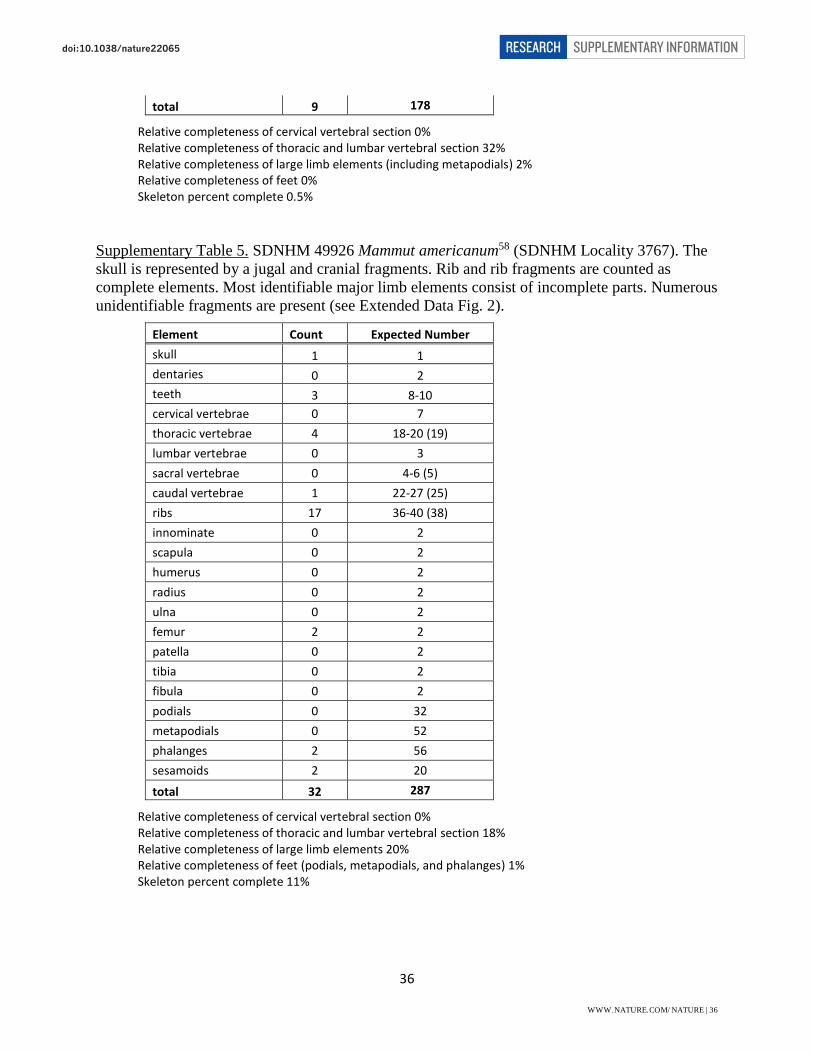
Supplementary Table 5. SDNHM 49926 Mammut americanum58 (SDNHM Locality 3767). The
skull is represented by a jugal and cranial fragments. Rib and rib fragments are counted as
complete elements. Most identifiable major limb elements consist of incomplete parts. Numerous
unidentifiable fragments are present (see Extended Data Fig. 2).
Element Count Expected Number
skull 1 1
dentaries 0 2
teeth 3 8-10
cervical vertebrae 0 7
thoracic vertebrae 4 18-20 (19)
lumbar vertebrae 0 3
sacral vertebrae 0 4-6 (5)
caudal vertebrae 1 22-27 (25)
ribs 17 36-40 (38)
innominate 0 2
scapula 0 2
humerus 0 2
radius 0 2
ulna 0 2
femur 2 2
patella 0 2
tibia 0 2
fibula 0 2
podials 0 32
metapodials 0 52
phalanges 2 56
sesamoids 2 20
total 32 287
Relative completeness of cervical vertebral section 0% Relative completeness of thoracic and lumbar vertebral section 18% Relative completeness of large limb elements 20% Relative completeness of feet (podials, metapodials, and phalanges) 1% Skeleton percent complete 11%
WWW.NATURE.COM/NATURE | 36
SUPPLEMENTARY INFORMATIONRESEARCHdoi:10.1038/nature22065

37
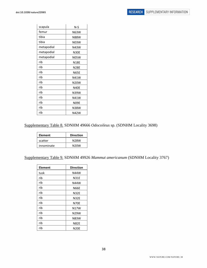
Supplementary Tables 6-9. Element Orientations. The azimuths of the long axes of individual
large limb bones from each specimen were measured from the quarry maps1 and/or from digital
scans of original copies of the excavation data on file at the SDNHM1. In curved tusks, ribs and
rib fragments of SDNHM 49926, measurements were taken parallel to a chord from one end of
the element to the other. Directions are recorded as north azimuths.
Supplementary Table 6. SDNHM 47731 Equus sp. (SDNHM Locality 3677)
Element Direction
humerus N07W
scapula N35E
radius/ulna N01E
innominate N03W
innominate N60W
femur N73W
tibia N63W
metapodial N88W
metapodial N51W
rib N52W
rib N52E
rib N78W
rib N71W
rib N61W
rib N80W
rib N54W
rib N87W
rib N24E
Supplementary Table 7. SDNHM 49012 Canis dirus (SDNHM Locality 3698)
Element Direction
dentary N56W
dentary N42W
humerus N03W
humerus N-S
radius N-S
ulna N58E
ulna N31W
WWW.NATURE.COM/NATURE | 37
SUPPLEMENTARY INFORMATIONRESEARCHdoi:10.1038/nature22065
38
scapula N-S
femur N63W
tibia N88W
tibia N03W
metapodial N43W
metapodial N30E
metapodial N05W
rib N18E
rib N28E
rib N65E
rib N41W
rib N20W
rib N40E
rib N39W
rib N41W
rib N09E
rib N38W
rib N42W
Supplementary Table 8. SDNHM 49666 Odocoileus sp. (SDNHM Locality 3698)
Element Direction
scatter N28W
innominate N20W
Supplementary Table 9. SDNHM 49926 Mammut americanum (SDNHM Locality 3767)
Element Direction
tusk N44W
rib N31E
rib N44W
rib N66E
rib N32E
rib N32E
rib N70E
rib N17W
rib N29W
rib N83W
rib N82E
rib N20E
WWW.NATURE.COM/NATURE | 38
SUPPLEMENTARY INFORMATIONRESEARCHdoi:10.1038/nature22065

39
SECTION 7. CERUTTI MASTODON SITE RADIOCARBON AND OPTICALLY STIMULATED
LUMINESCENCE DATING
Two attempts were made to radiocarbon date the CM site. The first attempt in the mid-
1990s involved submitting a tusk sample to Beta Analytic in Florida1. This dating attempt failed
when it was reported that the tusk fragment did not contain collagen. In 2009, a sample selected
from the interior dentine of a molar was submitted to Stafford Laboratories of Colorado. Again,
the sample did not contain collagen, so could not be dated.
An initial attempt to date the site by optically-stimulated luminescence (OSL) methods at
University of Illinois at Chicago (Steven L. Forman, written communication, 2016) was made in
2008 using samples collected for that purpose during the excavation in 1992-1993. Doses were
determined using the multiple-aliquot additive dose technique59, 60, 61. For polymineral fine-
grained separates, grains were first exposed to infrared light and then to blue light. Luminescence
output obtained under the initial infrared stimulation dominantly reflects feldspar components
whereas subsequent blue light stimulation reflects quartz components. Thus, samples UIC2287
and UIC2288 have two separate age estimates, designated by appending either “IR” (infrared
light) or “BL” (blue light) after the sample name in Supplementary Table 10. In contrast, data for
samples UIC2286 and a second aliquot of UIC2287 were determined from purified quartz
fractions obtained after soaking sediment for a week in hydrofluorosilicic acid. Grain-sizes
ranged from 63–100 µm for UIC2286 and from 4–11 µm for UIC2287. Equivalent doses for the
1992-1993 samples range from 241 to 270 Gy. Resulting OSL ages determined in 2008 range
from 69±9 ka to 99±12 ka (2σ uncertainties) with no statistically significant differences between
ages determined by infrared or blue light stimulation, or between polymineralic or pure quartz
aliquots (Supplementary Table 10). Significant age differences between Beds E and F were not
WWW.NATURE.COM/NATURE | 39
SUPPLEMENTARY INFORMATIONRESEARCHdoi:10.1038/nature22065

40
observed (weighted-mean age and 95% confidence limit of 73.3±4.1 ka for N=5 with a MSWD
[mean square weighted deviation] of 0.54), but the OSL age of 99±12 ka for the underlying unit,
Bed C, is discernably older.
A second attempt to date the fluvial sediment involved collection of OSL samples from a
nearby trench excavated in 2009 into the south side of the sound berm, about three meters from
the southeastern corner of the original CM site. The same sequence of stratified silt and sand
layers encountered in the 1992-1993 excavation was identified and OSL samples were collected
from Beds C, D, E and F by Steven Forman. Those samples were subjected to the same multiple-
aliquot additive dose methods used previously. Sediment from the trench excavated in 2009 was
coarser than sediment collected from the original CM site and contained abundant grains greater
than 250 microns in diameter. This difference is interpreted to represent lateral variation in
fluvial facies over the several meters separating the two sample sites. In addition, there appears
to be greater compositional heterogeneity in sediments from the 2009 excavation with total dose
rates derived from the U, Th and K concentrations varying by 50% (1.94 to 3.25 mGy/year). The
equivalent doses from the 2009 samples are about half those of the 2008 samples (>115 to >203
Gy versus 241 to 270 Gy), yet regenerative growth curves for those samples indicate that the
2009 samples are at or very close to saturation. Resulting ages for the 2009 samples are thus
reported as minimum ages ranging from >38 to >70 ka.
As a test of the multiple-aliquot additive dose method, a separate split of sample
UIC2585 was analyzed using a single-aliquot regeneration protocol59 on 30 aliquots of the 150-
to 250-micron quartz fraction. Resulting equivalent-dose measurements were within analytical
uncertainties generated for each method, and the resulting OSL age estimates for UIC2585 based
on both dose measurements were consistent (>62 ka and >70 ka).
WWW.NATURE.COM/NATURE | 40
SUPPLEMENTARY INFORMATIONRESEARCHdoi:10.1038/nature22065

41
To help resolve the differences between the 2008 and 2009 OSL dating results along with
the hope of obtaining an age from an independent laboratory, a set of sediment samples from the
original 1992-1993 collection was sent to Ronald J. Goble at the University of Nebraska in 2011.
Twelve individual aliquots from four separate samples representing Beds C, E, and F were
processed using pulsed irradiation60 and a 280°C shinedown59 as part of a single-aliquot
regeneration sequence. Equivalent doses ranged from 180±26 to 223±52 Gy (2σ uncertainties).
Most aliquots from all samples had equivalent doses (De) that exceeded the upper limits of the
saturation plateaus (De > 2×Do) and could not be dated (Ronald J. Goble, written communication,
2011). Those conclusions were determined on splits of the same material initially provided to the
University of Chicago laboratory.
Given results of the three attempts to date the sediments containing the mastodon bones
by OSL, we conclude that electron traps in the quartz and feldspar silt grains are close to or
beyond their saturation limits. Consequently, even though some individual samples may indicate
finite OSL ages, it is more likely that the material is too old to provide a reliable estimate of the
age of sediment deposition. We consider the best interpretation of the OSL data to be that
sediments representing the CM stratigraphy are greater than 60 to 70 ka. Although other
luminescence analytical approaches could be investigated, the apparent antiquity of the site along
with other factors inherent in dating of fluvial sediment, such as heterogeneity caused by facies
changes, variable sources of quartz within the deposits, and the potential for incomplete solar
resetting, will complicate any further efforts for luminescence dating.
WWW.NATURE.COM/NATURE | 41
SUPPLEMENTARY INFORMATIONRESEARCHdoi:10.1038/nature22065

42
Supplementary Table 10. Optically Stimulated Luminescence ages for fluvial sediments from the Cerutti
Mastodon Site determined in 2008.
Stratum Sample
numbera Anomalous fade ratiob
Equivalent dose (Gy)
U conc. (µg/g)c
Th conc.
(µg/g)c
K20 conc. (wt. %)c
a valued
Assumed H20
content (%)
Cosmic ray contribution
(mGy/yr)e
Total dose rate
(mGy/yr)
OSL age (ka)
Bed F UIC2288IR 0.99±0.06 241±8 2.2±0.2 6.7±0.2 1.97±0.04 0.062±0.012 10 ± 6 0.19±0.04 3.47±0.34 69±9
Bed F UIC2288BL 1.00±0.02 270±18 2.2±0.2 6.7±0.2 1.97±0.04 0.073±0.014 10 ± 6 0.19±0.04 3.56±0.34 76±10
Bed E UIC2287IR 1.03±0.02 251±3 2.5±0.2 6.6±0.2 1.51±0.02 0.075±0.016 10 ± 6 0.18±0.04 3.24±0.32 78±10
Bed E UIC2287BL 1.09±0.02 252±3 2.5±0.2 6.6±0.2 1.51±0.02 0.098±0.018 10 ± 6 0.18±0.04 3.42±0.32 73±9
Bed E UIC2287Qf ND 249±5 2.5±0.2 6.6±0.2 1.51±0.02 0.098±0.020 10 ± 6 0.18±0.04 3.43±0.34 72±9
Bed C UIC2286BLg ND 250±6 2.0±0.2 4.4±0.2 1.65±0.02 ND 5 ± 4 0.18±0.04 2.53±0.24 99±12
aThe BL designation indicates excitation by blue light (470 ± 20 nm) after exposure to infrared (IR) wavelengths (834 ± 80 nm) with the equivalent dose determined by the multiple-aliquot regenerative dose technique61.
bTest for anomalous fading of laboratory induced luminescence signal of approximately 99 Gy after 30 day storage at room temperature. Values of 0.90 to 1.10 indicate little to no fading within analytical resolution.
cU, Th and K20 concentrations (conc.) determined by ICP-MS at Activation Laboratories, Ontario, Canada.
dMeasured alpha-efficiency factor (a value) as defined by Aitken and Bowman62.
eAges included a cosmic ray dose rate from calculations of Prescott and Hutton63.
fData for sample UIC2287Q were determined on the 4- to 11-micron quartz fraction, isolated by reaction with hydrofluorosilic acid.
gData for sample UIC2286BL were determined on the 63- to 100-micron quartz fraction with blue light excitation (470 ± 20 nm); other analyses were made on the 4- to 11-micron polymineral fraction.
All errors given at two-times standard deviation. ND = not determined. Data obtained by Steven L. Forman at the University of Illinois at Chicago Luminescence Dating Research Laboratory.
WWW.NATURE.COM/NATURE | 42
doi:10.1038/nature22065 SUPPLEMENTARY INFORMATIONRESEARCH

43
Supplementary Table 11. Optically Stimulated Luminescence ages for fluvial sediments from the Cerutti
Mastodon Site determined in 2009.
Stratum Sample
numbera Equivalent dose (Gy)
U conc. (µg/g)b
Th conc. (µg/g)b
K20 conc. (wt. %)b
Assumed H20 content
(%)
Cosmic ray contributionc
(mGy/yr)
Total dose rate
(mGy/yr)
OSL age (ka)
Bed F UIC2588BL >203 ± 7 4.8 ± 0.2 10.6 ± 0.1 1.58 ± 0.04 10 ± 6 0.19 ± 0.04 3.25 ± 0.3 >62
Bed E UIC2586BL >115 ± 5 3.9 ± 0.2 9.2 ± 0.1 1.66 ± 0.04 10 ± 6 0.19 ± 0.04 3.03 ± 0.3 >38
Bed E2 UIC2585BLs >119 ± 21 1.4 ± 0.2 3.2 ± 0.1 1.50 ± 0.04 10 ± 6 0.18 ± 0.04 1.94 ± 0.2 >62
Bed E2 UIC2585BL >135 ± 6 1.4 ± 0.2 3.2 ± 0.1 1.50 ± 0.04 10 ± 6 0.18 ± 0.04 1.94 ± 0.2 >70
Bed D UIC2589BL >117 ± 3 2.3 ± 0.2 6.1 ± 0.1 1.59 ± 0.04 10 ± 6 0.18 ± 0.04 2.41 ± 0.2 >48
Bed C UIC2587BL >129 ± 7 3.0 ± 0.2 6.2 ± 0.1 1.62 ± 0.04 10 ± 6 0.18 ± 0.04 2.59 ± 0.3 >54
aThe BL designation indicates excitation by blue light (470 ± 20 nm) with the equivalent dose determined by the multiple-aliquot regenerative dose technique on the 150 to 250 micron quartz fraction (Jain et al. 2003). BLs designation indicates excitation by blue light (470 ± 20 nm) with equivalent dose determined by single-aliquot regeneration protocols59 on 30 aliquots of the 150-250 micron quartz fraction.
bU, Th and K20 determined by ICP-MS at Activation Laboratories, Ontario, Canada. cAges included a cosmic ray dose rate from calculations of Prescott and Hutton63. All errors given at two-times standard deviation. Data determined at the University of Illinois at Chicago Luminescence Dating
Research Laboratory.
WWW.NATURE.COM/NATURE | 43
doi:10.1038/nature22065 SUPPLEMENTARY INFORMATIONRESEARCH

44
SECTION 8. URANIUM-SERIES AGES
Because of the difficulties in dating sediment at the CM site using OSL methods, an
attempt was made to use uranium-series methods to date the bones themselves. Scoping efforts
were conducted at the U.S. Geological Survey radiogenic isotope lab in late 2011 to determine
whether material was amenable to the method. More detailed efforts followed in 2012 through
2015 to establish a robust minimum age of death and diagenetic U-uptake as described below
(see Methods section for analytical details).
Conventionally Calculated 230Th/U Ages
Conventionally calculated 230Th/U ages rely on measured 230Th/238U activity ratios (AR)
and 234U/238U AR data corrected for the presence of any non-authigenic component that would
contribute initial 230Th not derived from in-situ decay of U. Corrections are made based on
measured 232Th/238U AR and the assumptions that this material is uniform, has a known U/Th
composition (for instance, one similar to average crustal material), and is in radioactive secular
equilibrium64 (that is, an assumed composition of 230Th/238U AR = 1.276 ±0.64; 230Th/238U AR =
1.0 ±0.25; 234U/238U AR = 1.0 ±0.1). Uncertainties are propagated through the age calculation so
that errors for corrected ratios are only slightly larger than analytical uncertainties if the
measured 232Th/238U AR is negligible (say <<0.1), but may be large if substantial 232Th is present
(i.e., 232Th/238U AR >0.2). Initial Th-corrections were negligible for analyses of CM bone
relative to analytical uncertainties.
Conventionally calculated 230Th/U ages for individual analyses of cortical bone from
Bed E at the CM site (Spl.1, CM-20, CM-225, and CM-292) ranged from 100.5±0.7 to
126.9±1.1ka with calculated initial 234U/238U AR of 1.38–1.49 (Supplementary Table 12;
Extended Data Figs. 9e–g, 10a, and 10b). Analyses of bone collected from the initial backhoe
WWW.NATURE.COM/NATURE | 44
SUPPLEMENTARY INFORMATIONRESEARCHdoi:10.1038/nature22065

45
excavation (sample SDNHM-09) have systematically older conventional 230Th/U ages (up to
152.9±1.5 ka) compared to specimens collected from in situ contexts, but yielded initial
234U/238U AR values in the same range (Extended Data Fig. 10b). Because of the lack of specific
stratigraphic context, older ages for SDNHM-09 specimens may indicate that they are from a
deeper stratigraphic horizon, or may be an artifact of U-loss, which was not fully evaluated in
those bones.
Models of Uranium Uptake
Uranium-series dating methods have been successfully applied to samples of bone, but
not without a reasonable understanding of how uranium was incorporated into the samples65, 66,
67, 68, 69, 70. Seventy analyses of fossilized bone from the CM site have an average U concentration
of 162±67 (±2×standard deviation [SD]) µg/g compared to U concentrations of approximately
0.05 µg/g or less in bone tissue of living animals71, 72, 73. It is clear that large amounts of U have
been incorporated into the samples of CM porous carbonated hydroxyapatite after burial and
diagenesis. Therefore, conventional 230Th/U ages that assume closed-system conditions (no
addition or subtraction of mass since mineral formation) will underestimate the true age of
burial. Understanding the history of diagenetic addition of U is a major challenge in accurately
estimating the age of the site.
Bones that experience relatively simple U uptake can provide robust, defensible ages;
however, bones that experience more complex uptake histories involving multi-stage episodes of
adsorption and leaching are not good candidates for U-series dating66, 67. Evidence of reliable
dates include (1) U concentrations and conventional closed-system 230Th/U ages across a single
bone that yield predictable rather than irregular profiles, and (2) analyses of multiple bones from
the same stratigraphic horizon that give a narrow range of ages and initial 234U/238U AR values.
WWW.NATURE.COM/NATURE | 45
SUPPLEMENTARY INFORMATIONRESEARCHdoi:10.1038/nature22065

46
Additional confidence is gained if initial 234U/238U AR values from U-series results are consistent
with known U-isotopic compositions in local water sources, and if other materials less
susceptible to diagenetic modification yield similar age results. Analyses of other materials were
attempted, including Mammut tooth enamel and tusk, bones from small animals (Sylvilagus and
Reptilia), pedogenic rinds developed on cobble clasts and bones, and calcite-cemented casts of
roots or insect burrows. However, those other materials had lower U concentrations, were more
susceptible to secondary U mobility, or required large corrections for initial 230Th. Consequently,
results from those materials had greater uncertainties and were less reliable and consistent than
results obtained from thick cortical limb and rib bones.
U is readily soluble in shallow, oxidizing groundwater, and interaction between those
waters and the buried bone resulted in loss of much of the organic matter (collagen) and
incorporation of U within the carbonated hydroxyapatite. Patterns of U uptake can take
numerous forms depending on the degree of hydrologic saturation and water-migration history of
the site, the diffusive characteristics of the bone, and the uranium concentrations in the
diagenetic environment66. Two simple conceptualizations of U behavior include (1) early uptake,
where all U is acquired over a short time span (relative to the age of burial) and then held tightly
in place, and (2) linear uptake, where U uptake occurs slowly and continuously until the present.
Actual uptake histories are likely more complex. Examination of profiles of U concentration and
U-series ages across sections of compact (cortical) bone can offer insights into U uptake
processes.
The diffusion-adsorption model (DA model) was developed to explain observed profiles
of U concentrations and U-series ages in bone samples65, 66, 67. The model assumes that uranyl
complexes (UO2+2) in aqueous solutions are able to diffuse into porous compact bone and adsorb
WWW.NATURE.COM/NATURE | 46
SUPPLEMENTARY INFORMATIONRESEARCHdoi:10.1038/nature22065

47
into the mineral fraction of bone, facilitated by its large internal surface areas. Laboratory
experiments indicate that hydroxyapatite has a strong affinity for uranyl ions66 (partition
coefficients between 104 and 105). Therefore, U-uptake depends mostly on how rapidly U can
diffuse into a given bone and how effectively it is absorbed by the mineral substrate. Parameters
controlling the DA process include the diffusion coefficient in bone (D) and the volume
equilibrium constant (R) representing the amount of U absorbed per unit amount of solution66.
Values purported for D/R depend on variations in the diffusion coefficient, porosity, and the
mineral/water partition coefficients, as well as chemical and physical factors present in the burial
environment, but are typically on the order of 10-12 cm2/s (resulting in rapid uptake rates) and
10-14 cm2/s (resulting in slow uptake rates). In the DA model, once a bone reaches equilibrium
with U in groundwater, no further uptake occurs, provided diagenetic conditions remain
constant66. Because Th is not mobile in aqueous solutions nor incorporated into biologic tissue,
the presence of 230Th in fossil bone is mostly a consequence of radioactive decay of 234U.
More recently, the DA model has been modified to accommodate both diffusion of 238U
and 234U into the bone along with simultaneous decay of excess 234U derived from the ambient
water contributing U during the process74. This so-called diffusion-adsorption-decay (DAD)
model acknowledges that diffusion of U is a continuous process and describes the evolution of
238U, 234U, and 230Th activities when diffusion and decay process are coupled74. Practical
differences between the DA and DAD models are described by Grün et al.70. Unlike the DA
model, the DAD model does not require U-concentration profiles for age calculations, although
those data remain an important diagnostic tool for evaluating the U-uptake history and the
suitability of samples for U-series dating74. In general, U from migrating water is introduced into
the bone starting from the outer and inner surfaces and progressing toward its center. U uptake is
WWW.NATURE.COM/NATURE | 47
SUPPLEMENTARY INFORMATIONRESEARCHdoi:10.1038/nature22065
48
non-linear and proceeds more rapidly during earlier stages and less rapidly during later stages.
Addition of U in this manner results in -shaped concentration profiles that gradually flatten
with time until the bone reaches a composition in equilibrium with U in the source water. The
distribution of conventionally calculated 230Th/U ages will result in similar -shaped patterns,
with apparent ages decreasing towards the center of the bone66, 74. Regardless of which approach
is adopted (conventionally calculated, DA-, or DAD-model ages), U-series dates of bone
represent minimum burial ages provided that U leaching has not occurred66, 70.
Cerutti Mastodon Ages
Profiles of U concentrations and conventionally calculated 230Th/U ages for sampled
specimens (CM-20, CM-225, CM-292) all approximate the -shaped profiles expected for
continuous uptake of U from water enriched in 234U relative to 238U (Extended Data Fig. 10a).
Modern soil water or percolating vadose water was not available for analyses; however, modern
groundwater analyzed from the shallow saturated zone in a nearby Sweetwater Authority
municipal supply well had 234U/238U AR values of 1.446 and 1.538 (Supplementary Table 12).
The similarity of those values to initial 234U/238U AR values calculated for outer layers of bone
assuming closed-system behavior is viewed as evidence that 230Th/238U data in bone profiles
have not been affected substantially by post-depositional U leaching, and that conventional ages
are not erroneously old due to U loss.
DAD-model ages for three specimens were calculated using 234U/238U AR and 230Th/238U
AR data as a function of position for each subsample volume and the iDAD program74 (available
at http://www.iearth.org.au/codes/iDaD/). Algorithms implemented in iDAD constitute a forward
model that predicts U-series activity profiles across a bone given an age and diffusion
coefficient. To do this, the program uses an inversion process based on measured isotope and
WWW.NATURE.COM/NATURE | 48
SUPPLEMENTARY INFORMATIONRESEARCHdoi:10.1038/nature22065

49
position data to estimate age and diffusion properties along with estimates of uncertainty74. The
model assumes a constant supply of 234U/238U AR at the inner and outer surfaces of the bone
throughout the burial history, and consequently DAD ages are typically older than conventional
230Th/U ages calculated for the same data (http://www.iearth.org.au/codes/iDaD/).
Results of the iDAD inversion model allow fitting of maximum likelihood solutions to
the measured data. Fits for CM-20 and CM-225 profiles are poor, resulting in probability density
functions (PDFs) with wide 95% credible intervals and large age uncertainties (Extended Data
Fig. 10c). The PDFs for these two profiles are asymmetric, resulting in maximum likelihood ages
that are offset from the PDF peak. This feature is a result of the fact that the maximum likelihood
solution solves for the best fit considering multiple parameters including diffusivity coefficient,
age, and the 234U/238U AR of the external source74. Resulting maximum-likelihood ages are
137.0±5.6 ka for CM-20 and 126.4±5.5 ka for CM-225, which barely overlap at the 95%
confidence limit (Extended Data Fig. 10d). We assume that the poor fits observed in these two
samples are caused by inhomogeneous diffusivity across the cortical layer rather than by U loss
because U concentration profiles show no evidence of lower values near layer margins
(Extended Data Fig. 10a).
In contrast, predicted values of 234U/238U AR and 230Th/238U AR more closely match
measured values for specimen CM-292. Consequently, the PDF curve is symmetric and yields a
narrower 95% credible interval half width. The resulting maximum-likelihood age of 130.2±2.7
ka corresponds to the peak of the PDF curve and is within error overlap of ages from the other
two specimens (Extended Data Fig. 10c).
WWW.NATURE.COM/NATURE | 49
SUPPLEMENTARY INFORMATIONRESEARCHdoi:10.1038/nature22065

50
Equilibrium 234U/238U ratios and apparent correlations with age
Equilibrium 234U/238U AR values calculated using the iDAD model range from 1.322 to
1.331 for all three specimens. Those values are lower than initial 234U/238U AR calculated using
conventional methods (1.38–1.49, see above). The lower equilibrium 234U/238U values calculated
from the DAD model are closer to present-day measured values than conventionally calculated
initial 234U/238U AR due to the assumption that U was introduced into the sample throughout its
burial history, and that the composition of the introduced U remained constant over the entire
period. As 234U is continually introduced, 234U decays within the bone and results in
accumulation of 230Th daughter; however, newly absorbed U replaces the decayed 234U so that
230Th increases without the same amount of apparent 234U loss required under closed conditions.
However, diffusion rates are low enough that U introduced from the environment loses
some of its original 234U through decay prior to reaching the center of the bone. Consequently, U
in the interior of the cortical bone has a lower 234U/238U AR than the margin. The result of this
phenomenon is apparent in Extended Data Fig. 10b, which shows positive correlations between
234U/238U AR and 230Th/238U AR in bone profiles. At face value, subsamples at bone margins
with the oldest conventionally calculated ages also have the highest initial 234U/238U AR values,
and subsamples from the interior have younger ages and lower initial 234U/238U AR.
Consequently, 234U/238U AR at the margins of the bone more closely reflects the composition of
U in the diagenetic environment. If the DAD model and its assumptions are correct, U in soil
water at the CM horizon has an isotopic composition that is lower than values measured in
shallow groundwater from the supply well just down-gradient from the site. In other thick vadose
zones, surface-flow, soil water, and shallow infiltration commonly have 234U/238U AR values
WWW.NATURE.COM/NATURE | 50
SUPPLEMENTARY INFORMATIONRESEARCHdoi:10.1038/nature22065

51
lower than those observed in underlying groundwater75 due to preferential incorporation of
recoil-generated 234U as infiltration percolates to greater depths.
Geochronological Conclusions
We interpret the U-series isotope data from systematic profiles across specimen CM-292
and its maximum likelihood model age of 130.2±2.7 ka calculated using the diffusion-
adsorption-decay (DAD) model74 to best represent the age of the CM horizon. Similarly,
calculated ages for profiles of the other two specimens are less well defined and have greater
uncertainties (137.0±5.6 ka and 126.4±5.5 ka). However, all three age estimates are within error
overlap at the 95% confidence level, and support an approximate 130 ka burial age (weighted
mean value of 130.7±9.4 ka using errors for the three individual determinations; Extended Data
Fig. 10d). Isotope data are consistent with conceptual models of gradual diffusion and absorption
of U into interior portions of cortical bone, and show no obvious evidence for post-burial U
leaching that would result in modified 230Th/238U AR values and erroneously old ages. Maximum
likelihood model ages are only marginally older than conventionally calculated 230Th/U ages for
individual analyses of subsamples from inner and outer layers of the cortical bones.
Conventionally calculated initial 234U/238U AR values are consistent with U present in shallow
groundwater from nearby wells, although the DAD model indicates that U in shallow infiltration
that contributed U to mineral components of the bone may have had a somewhat lower value.
The internal consistency of the age and initial 234U/238U AR data are interpreted as strong
evidence that bones have not been subject to post-depositional U leaching.
We conclude that the 230Th/U dates obtained for CM bone are minimum estimates of the
burial age rather than erroneously old artifacts caused by complex post-depositional U mobility.
The combined data indicate that mortality and burial very likely occurred at least 130,000 years.
WWW.NATURE.COM/NATURE | 51
SUPPLEMENTARY INFORMATIONRESEARCHdoi:10.1038/nature22065

52
This age estimate is consistent with geologic interpretations based on dated paleo shoreline
terraces (inboard of the 120-ka-aged Nestor Terrace) and the fact that the sedimentary
environment was one of aggradation rather than incision, likely facilitated by a high sea-stand
during MIS 5e. It is also compatible with radiocarbon results which indicate that bone is old
enough for all of its original collagen to have been removed (not a strict geochronological limit),
and with optically stimulated luminescence results, which are interpreted as evidence that
sediments enclosing the bone are older than 60 to 70 ka.
WWW.NATURE.COM/NATURE | 52
SUPPLEMENTARY INFORMATIONRESEARCHdoi:10.1038/nature22065

53
Supplementary Table 12. U-Th concentrations, isotopic compositions, and conventionally calculated 230Th/U ages and initial 234U/238U
activity ratios for samples of bone and pedogenic carbonate from the Cerutti Mastodon site, and U concentrations and 234U/238U
activity ratios for shallow groundwater from Sweetwater Authority well SW, San Diego County, California.
Sample Name Sample weight
(g)
Depth from outer
surface (mm)
U conc. (µg/g)
Th conc. (µg/g)
Measured activity ratios Detritus-corrected activity ratios 230Th/U
Agec ±2σ (ka)
Initial 234U/238U
activity ratioc ±2σ
232Th/ 238U activity ratioa,b ±2σ
230Th/ 238U activity ratioa,b ±2σ
234U/238U activity ratioa,b
±2σ
230Th/ 232Th
activity ratioa
230Th/ 238U activity ratioa,b ±2σ
234U/238U activity ratioa,b
±2σ
Mastodon rib bone; Locale #3767 bed E; Specimen #49926; Rib fragment; collected from backhoe excavation, northeast corner of site
Spl.1A 0.0168 0.5-1.5 130.5 0.038 9.1E-5±9.0E-6 0.9017±0.0036 1.3118±0.0029 9,910 0.9017±0.0036 1.3118±0.0029 118.7±0.9 1.436±0.004
Spl.1B 0.0543 2.2-4.1 132.9 0.013 2.8E-5±2.8E-6 0.8868±0.0035 1.3063±0.0028 31,226 0.8868±0.0035 1.3063±0.0028 116.3±0.9 1.425±0.004
Spl.1C 0.0465 0.2-3.5 132.7 0.024 5.5E-5±3.2E-6 0.8942±0.0038 1.314±0.0029 16,348 0.8942±0.0038 1.314±0.0029 116.6±1.0 1.436±0.004
Spl.1D 0.0977 4.5-6.5 113.7 0.032 8.7E-5±1.8E-6 0.8611±0.0036 1.2958±0.0028 9,897 0.8611±0.0036 1.2959±0.0028 112.4±0.9 1.406±0.003
Various bones; Locale #3767; Specimens collected from backhoe excavation in northeast corner of site
SDNHM-09A-1 0.0441 1.5-2.7 94.6 0.021 6.9E-5±3.6E-6 0.9737±0.0041 1.2925±0.0028 14,091 0.9737±0.0041 1.2926±0.0028 140.5±1.3 1.435±0.004
SDNHM-09A-2 0.0208 2.7-4.7 83.6 0.033 1.2E-4±8.7E-6 0.9520±0.0038 1.2821±0.0028 7,689 0.9519±0.0038 1.2821±0.0028 137.0±1.2 1.415±0.004
SDNHM-09A-3 0.0548 4.7-6.0 85.8 0.028 1.0E-4±3.2E-6 0.9362±0.0038 1.2786±0.0027 9,243 0.9362±0.0038 1.2786±0.0027 133.5±1.2 1.406±0.003
SDNHM-09A-4 0.0139 6.0-7.5 91.8 0.079 2.8E-4±1.2E-5 0.9265±0.0055 1.2859±0.0089 3,323 0.9265±0.0055 1.2859±0.0089 129.5±2.3 1.412±0.011
SDNHM-09A-5 0.0137 7.5-9.0 89.6 0.043 1.5E-4±1.2E-5 0.9123±0.0038 1.2773±0.0034 5,992 0.9123±0.0038 1.2773±0.0034 127.6±1.2 1.398±0.004
SDNHM-09B-1 0.0460 1.2-3.2 163.5 0.026 4.7E-5±2.0E-6 0.8558±0.0034 1.318±0.0028 18,035 0.8558±0.0034 1.318±0.0028 107.9±0.8 1.431±0.003
SDNHM-09C-1 0.0413 3.0-5.2 145.1 0.010 1.7E-5±2.5E-6 1.0351±0.0048 1.3287±0.0031 60,095 1.0351±0.0048 1.3287±0.0031 148.9±1.6 1.500±0.004
SDNHM-09C-2 0.0245 5.2-7.2 140.4 0.013 2.6E-5±4.4E-6 1.0163±0.0042 1.3245±0.0032 39,772 1.0163±0.0042 1.3245±0.0032 144.7±1.4 1.488±0.004
SDNHM-09E-1 0.0277 5-9 165.1 0.013 2.1E-5±3.3E-6 0.9871±0.0039 1.2599±0.0028 46,006 0.9871±0.0039 1.2599±0.0028 152.9±1.5 1.400±0.004
CM-20: Mastodon rib bone with intact head on one end and sharp fracture on opposite end; Locale #3767 bed E; Specimen #49926; Field #20
CM-20-01 0.0205 0.5 163.1 0.050 9.6E-5±4.5E-6 0.9567±0.0037 1.342±0.0031 10,011 0.9567±0.0037 1.342±0.0031 125.9±1 1.488±0.004
CM-20-02 0.0332 1.5 152.7 0.009 1.4E-5±3.0E-6 0.9569±0.0039 1.337±0.0028 67,384 0.9569±0.0039 1.337±0.0028 126.9±1.1 1.482±0.004
CM-20-03 0.0242 2.5 145.6 0.009 1.5E-5±4.3E-6 0.9447±0.0036 1.3312±0.0028 64,109 0.9447±0.0036 1.3312±0.0028 125.1±1 1.471±0.004
CM-20-04 0.0213 3.5 133.5 0.023 5.3E-5±5.3E-6 0.9497±0.0039 1.3293±0.003 17,980 0.9497±0.0039 1.3293±0.0030 126.6±1.1 1.471±0.004
CM-20-05 0.0209 4.5 132.9 0.010 2.1E-5±5.5E-6 0.9232±0.0035 1.3285±0.0028 44,268 0.9232±0.0035 1.3285±0.0028 120.7±0.9 1.462±0.003
WWW.NATURE.COM/NATURE | 53

54
CM-20-06 0.0269 5.5 131.0 0.015 3.3E-5±4.3E-6 0.8886±0.0034 1.3245±0.0028 27,039 0.8886±0.0034 1.3245±0.0028 113.7±0.9 1.447±0.003
CM-20-07 0.0348 6.5 129.3 0.009 1.8E-5±3.4E-6 0.9185±0.0036 1.3226±0.0028 50,815 0.9185±0.0036 1.3226±0.0028 120.6±1 1.453±0.003
CM-20-08 0.0273 7.5 118.4 0.016 3.9E-5±4.7E-6 0.8615±0.0034 1.3223±0.0028 22,222 0.8615±0.0034 1.3223±0.0028 108.4±0.8 1.438±0.003
CM-20-09 0.0246 8.5 116.6 0.015 3.8E-5±5.3E-6 0.9156±0.0038 1.3178±0.0028 24,327 0.9156±0.0038 1.3178±0.0028 120.8±1 1.447±0.004
CM-20-10 0.0284 9.5 116.4 0.020 5.2E-5±4.6E-6 0.9068±0.0035 1.3097±0.0029 17,280 0.9068±0.0035 1.3097±0.0029 120.2±1 1.435±0.004
CM-20-11 0.0228 10.5 125.2 0.015 3.5E-5±5.3E-6 0.9161±0.0040 1.3107±0.0029 25,954 0.9161±0.0040 1.3107±0.0029 122.2±1.1 1.439±0.004
CM-20-12 0.0299 11.5 131.8 0.014 3.1E-5±3.8E-6 0.8841±0.0034 1.3096±0.0028 28,083 0.8841±0.0034 1.3096±0.0028 115.2±0.9 1.428±0.003
CM-20-13 0.0261 12.5 133.1 0.013 2.7E-5±4.4E-6 0.9367±0.0038 1.3260±0.0028 34,241 0.9367±0.0038 1.326±0.0028 124.2±1 1.463±0.003
CM-225: Mastodon limb bone with spiral fracture; Locale #3767 bed E; Specimen #49926; Field #225
CM-225-01 0.0187 0.5 203.8 0.118 1.9E-4±4.0E-6 0.8947±0.0037 1.3447±0.0031 4,809 0.8947±0.0037 1.3448±0.0031 111.9±0.9 1.473±0.004
CM-225-02 0.0103 1.5 193.0 0.023 3.5E-5±7.7E-6 0.8698±0.0034 1.3364±0.0028 24,940 0.8698±0.0034 1.3364±0.0028 108.0±0.8 1.456±0.003
CM-225-03 0.0087 2.5 195.7 0.022 3.2E-5±8.9E-6 0.8647±0.0034 1.3225±0.0029 26,864 0.8647±0.0034 1.3225±0.0029 109.0±0.8 1.439±0.004
CM-225-04 0.0123 3.5 193.9 0.016 2.3E-5±6.4E-6 0.8594±0.0033 1.3194±0.0028 37,459 0.8594±0.0033 1.3194±0.0028 108.4±0.8 1.434±0.003
CM-225-05 0.0188 4.5 190.9 0.008 9.0E6±4.2e-6 0.8634±0.0033 1.3221±0.0028 101,547 0.8634±0.0033 1.3221±0.0028 108.8±0.8 1.438±0.003
CM-225-06 0.0185 5.5 185.1 0.009 1.1E-5±4.4E-6 0.831±0.0034 1.3195±0.003 72,687 0.8310±0.0034 1.3195±0.0030 102.7±0.8 1.427±0.004
CM-225-07 0.0224 6.5 183.2 0.008 1.1E-5±3.7E-6 0.85±0.0034 1.32±0.0029 80,679 0.8500±0.0034 1.3200±0.0029 106.4±0.8 1.432±0.004
CM-225-08 0.0244 7.5 179.5 0.008 1.1E-5±3.5E-6 0.8129±0.0032 1.3089±0.0027 73,227 0.8129±0.0032 1.3089±0.0027 100.5±0.7 1.410±0.003
CM-225-09 0.0201 8.5 183.4 0.006 7.0E-6±4.1E-6 0.8458±0.0034 1.3006±0.0028 121,794 0.8458±0.0034 1.3006±0.0028 108.4±0.8 1.408±0.003
CM-225-10 0.0209 9.5 184.8 0.009 1.2E-5±3.9E-6 0.8381±0.0032 1.2848±0.0027 71,338 0.8381±0.0032 1.2848±0.0027 109.2±0.8 1.388±0.003
CM-225-12 0.0224 11.5 192.1 0.007 8.0E-6±3.5E-6 0.849±0.0035 1.2727±0.0027 102,933 0.8490±0.0035 1.2727±0.0027 113.5±0.9 1.376±0.003
CM-225-15 0.0209 14.5 197.6 0.008 8.0E-6±3.7E-6 0.8618±0.0033 1.2935±0.0028 107,659 0.8618±0.0033 1.2935±0.0028 112.9±0.9 1.404±0.003
CM-225-18 0.0211 17.5 195.7 0.013 1.6E-5±3.7E-6 0.875±0.0036 1.3166±0.0028 53,415 0.8750±0.0036 1.3166±0.0028 112.1±0.9 1.434±0.003
CM-225-20 0.0268 19.5 196.3 0.021 3.1E-5±2.9E-6 0.9022±0.0036 1.3297±0.0028 29,277 0.9022±0.0036 1.3297±0.0028 115.8±0.9 1.457±0.003
CM-292: Mastodon limb bone; Locale #3767 bed E; Specimen #49926; Field #292
CM-292-01 0.0109 0.25 198.8 0.365 6.0E-4±7.3E-6 0.9065±0.0044 1.3294±0.0028 1,511 0.9064±0.0044 1.3296±0.0028 116.7±1.1 1.458±0.004
CM-292-02 0.0097 0.5 195.1 0.059 9.5E-5±8.0E-6 0.9074±0.0042 1.3338±0.0028 9,558 0.9074±0.0042 1.3338±0.0028 116.3±1 1.463±0.004
CM-292-03 0.0151 1 187.5 0.039 6.4E-5±5.4E-6 0.8919±0.0037 1.3208±0.0027 14,040 0.8919±0.0037 1.3208±0.0027 115.0±0.9 1.444±0.003
CM-292-04 0.0153 1.3 183.6 0.041 6.8E-5±5.4E-6 0.8915±0.0042 1.3212±0.0028 13,059 0.8915±0.0042 1.3212±0.0028 114.9±1 1.444±0.003
CM-292-05 0.0141 2 181.7 0.033 5.5E-5±5.9E-6 0.8891±0.0035 1.3233±0.0029 16,068 0.8891±0.0035 1.3233±0.0029 114.0±0.9 1.446±0.004
CM-292-06 0.0156 2.3 180.0 0.028 4.6E-5±5.4E-6 0.8833±0.0042 1.3162±0.0039 19,162 0.8833±0.0042 1.3162±0.0039 113.9±1.1 1.436±0.005
CM-292-07 0.0133 3 274.3 0.046 5.0E-5±4.1E-6 0.8725±0.0033 1.3115±0.0027 17,340 0.8725±0.0033 1.3116±0.0027 112.3±0.8 1.428±0.003
WWW.NATURE.COM/NATURE | 54

55
CM-292-08 0.0177 3.75 177.6 0.022 3.7E-5±4.8E-6 0.8729±0.0034 1.3123±0.0028 23,823 0.8729±0.0034 1.3123±0.0028 112.3±0.9 1.429±0.003
CM-292-09 0.0151 4.5 174.4 0.022 3.7E-5±5.7E-6 0.8618±0.0037 1.3101±0.0028 23,344 0.8618±0.0037 1.3101±0.0028 110.3±0.9 1.423±0.003
CM-292-10 0.0143 5.25 174.4 0.024 4.1E-5±6.1E-6 0.8563±0.0033 1.3012±0.0027 20,806 0.8563±0.0033 1.3012±0.0027 110.5±0.8 1.411±0.003
CM-292-11 0.0136 6.2 170.5 0.029 5.2E-5±6.6E-6 0.8537±0.0034 1.3065±0.0030 16,394 0.8537±0.0034 1.3065±0.0030 109.1±0.8 1.417±0.004
CM-292-12 0.0127 7 166.9 0.022 3.9E-5±7.1E-6 0.8520±0.0036 1.3117±0.0031 21,991 0.8520±0.0036 1.3117±0.0031 108.0±0.9 1.423±0.004
CM-292-13 0.0128 7.9 165.2 0.025 4.6E-5±7.2E-6 0.8513±0.0032 1.3058±0.0027 18,404 0.8513±0.0032 1.3058±0.0027 108.7±0.8 1.416±0.003
CM-292-14 0.0157 8.8 162.7 0.021 3.9E-5±5.9E-6 0.8452±0.0033 1.3101±0.0028 21,934 0.8452±0.0033 1.3101±0.0028 106.8±0.8 1.419±0.003
CM-292-15 0.0162 9.5 166.4 0.017 2.8E-5±5.6E-6 0.8470±0.0034 1.3076±0.0030 29,957 0.847±0.0034 1.3076±0.0030 107.6±0.8 1.417±0.004
CM-292-16 0.0127 10.3 165.3 0.023 4.1E-5±7.2E-6 0.8438±0.0032 1.3104±0.0027 20,572 0.8438±0.0032 1.3104±0.0027 106.5±0.8 1.419±0.003
CM-292-17 0.0137 11.1 167.2 0.025 4.5E-5±6.6E-6 0.8464±0.0041 1.3090±0.0027 18,796 0.8463±0.0041 1.3090±0.0027 107.2±0.9 1.418±0.003
CM-292-18 0.0133 12 170.4 0.024 4.2E-5±6.7E-6 0.8521±0.0048 1.3081±0.0030 20,261 0.8521±0.0048 1.3081±0.0030 108.6±1.1 1.419±0.004
CM-292-19 0.0029 13 173.6 0.206 3.9E-4±3.1E-5 0.8779±0.0153 1.3100±0.0047 2,277 0.8779±0.0153 1.3101±0.0047 113.7±3.4 1.427±0.007
CM-292-20 0.0039 13.9 172.1 0.107 2.0E-4±2.3E-5 0.8769±0.0063 1.3100±0.0028 4,378 0.8769±0.0063 1.3101±0.0028 113.5±1.4 1.427±0.004
CM-292-21 0.0166 14.7 173.7 0.022 3.7E-5±5.3E-6 0.8680±0.0034 1.3119±0.0029 23,615 0.8680±0.0034 1.3119±0.0029 111.3±0.9 1.427±0.004
CM-292-22 0.0147 15.7 176.3 0.028 4.7E-5±5.8E-6 0.8735±0.0037 1.3120±0.0027 18,609 0.8735±0.0037 1.3120±0.0027 112.5±0.9 1.429±0.003
CM-292-23 0.0142 16.7 176.7 0.070 1.2E-4±6.1E-6 0.8806±0.0046 1.3145±0.0027 7,025 0.8806±0.0046 1.3146±0.0027 113.6±1.1 1.433±0.003
CM-292-24 0.0137 17.5 179.1 0.029 4.8E-5±6.2E-6 0.8673±0.0035 1.3216±0.0030 18,078 0.8672±0.0035 1.3216±0.0030 109.7±0.9 1.438±0.004
CM-292-25 0.0150 18.2 171.0 0.034 6.1E-5±5.9E-6 0.8963±0.0036 1.3219±0.0030 14,733 0.8963±0.0036 1.3219±0.0030 115.8±0.9 1.446±0.004
CM-292-26 0.0145 19.5 179.4 0.030 5.0E-5±5.8E-6 0.8805±0.0034 1.3217±0.0029 17,748 0.8805±0.0034 1.3217±0.0029 112.4±0.8 1.442±0.004
CM-292-27 0.0154 20.5 180.8 0.043 7.3E-5±5.5E-6 0.9069±0.0037 1.3298±0.0028 12,375 0.9069±0.0037 1.3298±0.0028 116.8±0.9 1.459±0.003
CM-292-28 0.0140 21.3 181.7 0.071 1.2E-4±6.0E-6 0.9131±0.0035 1.3341±0.0028 7,372 0.9131±0.0035 1.3342±0.0028 117.4±0.9 1.466±0.003
CM-292-29 0.0088 22 165.4 0.207 4.1E-4±1.1E-5 0.9238±0.0044 1.3395±0.0029 2,262 0.9238±0.0044 1.3396±0.0029 118.9±1.1 1.475±0.004
CM-292-30 0.0121 22.8 159.6 0.462 9.5E-4±8.2E-6 0.9574±0.0038 1.3386±0.0029 1,008 0.9573±0.0038 1.3389±0.0029 126.6±1.1 1.484±0.004
Shallow groundwater from Sweetwater Authority water well SW, zones 5 and 6; 32.65889°N, -117.0855571°; Samples collected 10/15-16/2009
SDSW5 105.663 0.00084 1.446±0.003
SDSW6 44.803 0.00338 1.538±0.004
WWW.NATURE.COM/NATURE | 55

56
SECTION 9. ASIAN ORIGINS OF EARLY HUMANS ON THE WEST COAST OF NORTH AMERICA
Climatic conditions during the last interglacial period (Marine Isotope Stage 5e [MIS 5e])
would have allowed entry of early hominins into North America76. This was the warmest
interglacial period in the middle and late Pleistocene and one of the warmest during the entire
Pleistocene Epoch. This period of global climatic warming allowed vertebrates from mid-latitude
North America to range into more northerly latitudes and to higher elevations. For example,
mastodons and sloths dispersed north above the Arctic Circle in Alaska, USA and the Yukon,
Canada77 and moved to higher elevations in the Rocky Mountains. After glacial retreat near the
end of MIS 6 and the beginning of MIS 5 these taxa lived at an elevation of 2705 m (amsl) in
central Colorado, USA78, representing their northern-most limit in North America, as well as the
highest elevation record for sloth and the second highest record for mastodons. Related to this
northward movement of mammals is the discovery of a single capybara (Hydrochoerus) tooth
(SDNHM 143879) at the CM site. This is the northwestern-most record for the genus and is far
outside of its modern range in South America and northwest of the late Pleistocene distribution
of capybara in northeastern Sonora, Mexico79. The occurrence of capybara at the CM site
suggests a warmer and wetter climate in this area at that time, conditions consistent with those of
MIS 5e.
Hominins in Eurasia during MIS 5 include Homo sapiens, Homo neanderthalensis, Homo
sp. (Denisova), Homo floresiensis and Homo erectus80, 81. These taxa, except Homo floresiensis,
could have dispersed into northeastern Asia as temperatures increased at the end of MIS 6 and
during the Last Interglacial MIS 582. Plausible dispersal routes for hominins to arrive on the west
coast of North America at the end of MIS 6 include a land route across Beringia prior to 135 ka83
and a coastal water route along the coasts of Asia, Beringia and North America. If Beringia was
WWW.NATURE.COM/NATURE | 56
SUPPLEMENTARY INFORMATIONRESEARCHdoi:10.1038/nature22065

57
partially submerged, the inland route would have required traversing a narrow water passage
separating present-day Siberia from Alaska; a maximum of an 80-km crossing with Diomede
Islands midway.
The continuous presence of hominins beginning ~300 ka in southern Siberia at the end of
the Lower Paleolithic, although many of the sites are not well-dated84, provides a potential
source of populations that could disperse eastward. By adapting to conditions in southern
Siberia, hominins could have extended their range further northeast to cross Beringia during
interglacial intervals. The southern edge of the Beringian land bridge at its maximum extent is
estimated to have been close to 63° N, about 200 km further north than the Diring Yuriakh site
situated at 60° N in Siberia. The best age estimate for the lower level of the site containing stone
tools is based upon TL dates of 267-366 ka85. However, the geoarchaeological position and age
(especially of the oldest stone artefacts) have been questioned86. It is noteworthy that fossil
remains of a cold-adapted female hominin, possibly an archaic Homo sapiens, have been
discovered in Manchuria, China (40° 34ʹ N). Animal teeth at the site were dated to ~ 260 ka by
electron-spin resonance and uranium series dating87. It is not yet known how far north these cold-
adapted hominins dispersed, but they may be responsible for archaeological sites like Diring
Yuriakh and other Early Paleolithic sites in southern Siberia.
At Denisova Cave (51.4° N) in southcentral Siberia, Homo neanderthalensis is first
evidenced by the appearance of Middle Paleolithic stone tools in Stratum 22 with bracketing
radio thermoluminescence (RTL) ages of 282 ± 56 and 171 ± 43 ka88. Biostratigraphic and
paleomagnetic data (Blake polarity episode) correlate more recent Denisova Cave Middle
Paleolithic stone tool industries with MIS 586. Thus, there are several possible hominin
candidates (late Homo erectus, Neanderthals or archaic Homo sapiens) resident in eastern Asia
WWW.NATURE.COM/NATURE | 57
SUPPLEMENTARY INFORMATIONRESEARCHdoi:10.1038/nature22065

58
that could have entered North America via Beringia and dispersed to the west coast of North
America at 130 ka. Another possibility is that the little-known Denisovans, related most closely
to Neanderthals89, and known only from DNA studies at Denisova Cave, were the first hominins
to reach North America.
In support of a coastal dispersal route is indirect evidence for the use of watercraft by
hominins more than 100 ka. For example, the biogeographic barrier in Southeast Asia called the
Wallace Line is marked by a deep ocean trench that limits most terrestrial species from
dispersing from mainland Asia and western Indonesia to islands in eastern Indonesia. However,
hominins crossed this barrier at least two times before 100 ka. The oldest recorded evidence is
the presence of stone tools dating to 1.1 Ma90 (probably made by ancestors of Homo floresiensis)
on the island of Flores (lowest sea level sea crossing at Lombok Strait, ~19 km91). Additional
evidence is provided by the presence of stone tools made by archaic humans (possibly H. erectus,
or Homo sp. (Denisova)) at sites on the island of Sulawesi (lowest sea level sea crossing at
Makassar Strait, ~ 42 km91) dating to between 118 and 194 ka92. In the Mediterranean Sea, there
is evidence of an early hominin reaching Crete more than 130 ka based on the presence of
Palaeolithic artefacts found there93. Thus, early hominins using watercraft appear to have had the
capacity to cross relatively narrow expanses of ocean before 100 ka ago. Based on this capacity,
early hominins could have followed the east coast of Asia northward as the climate warmed at
the beginning of MIS 5. They then could have followed the southern coast of Beringia, or
crossed a short distance of open water between present-day Siberia and Alaska if the land
connection had recently been submerged. A route south along the west coast of North America
would then have brought them to the latitude of the CM site.
WWW.NATURE.COM/NATURE | 58
SUPPLEMENTARY INFORMATIONRESEARCHdoi:10.1038/nature22065

59
Three hominin groups are candidates for making the journey to North America by simple
watercraft during the latest middle Pleistocene80. The first is an archaic human (Homo
neanderthalensis, Homo sp. (Denisovans) or Homo erectus). Neanderthals and “Denisovans”
were probably present in northeastern Asia during MIS 5, and potentially capable of sea
crossings. Homo erectus or their descendants were present in eastern mainland Asia at this time
with potential sea-crossing capacity, since they are candidates for reaching the islands of Flores
and Sulawesi90, 91, 92. A more remote possibility is that Homo sapiens made the journey. Recent
discoveries suggest that Homo sapiens was present in southern China sometime between 80 and
120 ka94, 95. The CM site is well-dated to 130.7 +/- 9.4 ka. This time period is consistent with the
onset of sea-level high stand conditions during MIS 5e dated by corals from tectonically stable
areas96, 97, 98. Higher temperatures and rapid sea-level rises associated with Termination II
deglaciation may have facilitated coastal migration routes.
Another possible hominin group making the journey to North America is identified by
DNA studies of remote Native Americans in Amazonia and the Central Brazilian Plateau. This
study found traces of DNA from an unknown Population Y related to Australasians99, 100. This
DNA type is not present in Mesoamerican or North American Native American populations. The
authors state “The arrival of Population Y ancestry in the Americas must in any scenario have
been ancient: while Population Y shows a distant genetic affinity to Andamanese, Australian and
New Guinean populations, it is not particularly closely related to any of them, suggesting that the
source of Population Y in Eurasia no longer exists; furthermore, we detect no long-range
admixture linkage disequilibrium in Amazonians as would be expected if the Population Y
migrations had occurred within the last few thousand years.” This earlier dispersal event appears
to be unrelated to the migration or migrations of later populations that became the Native
WWW.NATURE.COM/NATURE | 59
SUPPLEMENTARY INFORMATIONRESEARCHdoi:10.1038/nature22065
Americans and therefore must have occurred at an earlier date. Thus, Population Y, a group
distantly related to modern Australasians but with no modern analog population in southeast
Asia or Australia, may have arrived in the Americas quite early. Of course, Population Y could
be the same early Homo sapiens group discussed previously.
The CM site currently is the only locality in North America that supports such an early
hominin dispersal. This speculative discussion poses the challenge to initiate archaeological
research in MIS 5e and MIS 6-age geological deposits in North America.
SECTION 10. REFERENCES CITED IN SUPPLEMENTARY INFORMATION SECTIONS
1. Deméré, T.A., Cerutti, R.A. & Majors, C.P. State Route 54 Paleontological Mitigation
Program: Final Report. (San Diego Natural History Museum, 1995).
2. Kennedy, M.P. & Tan, S.S. Geology of National City, Imperial Beach, and Otay Mesa
quadrangles, southern San Diego Metropolitan area, California. Calif. Div. Mines and
Geology, Map Sheet 29 (1977).
3. Kern, J.P. Origin and history of upper Pleistocene marine terraces, San Diego, California.
Bull. Geol. Soc. Amer. 88, 1553-1566 (1977).
4. Kern, J.P. & Rockwell, T.K. in Quaternary Coasts of the United States: Marine and
Lacustrine Systems (eds C.H. Fletcher, III and J.F. Wehmiller), 377-382 (SEPM Special
Publication 48 1992).
5. Ku, T-L. & Kern J.P. Uranium-series age of the upper Pleistocene Nestor terrace, San
Diego, California. Bull. Geol. Soc. Amer. 85, 1713-1716 (1974).
6. Kraus, M.J. & Hasiotis, S.T. Significance of different modes of rhizolith preservation to
interpreting paleoenvironmental and paleohydrologic settings: Examples from Paleogene
WWW.NATURE.COM/NATURE | 60
SUPPLEMENTARY INFORMATIONRESEARCHdoi:10.1038/nature22065

paleosols, Bighorn Basin, Wyoming, U.S.A. J. of Sedimentary Research. 76, 633-646
(2006).
7. Holen, S.R. & Talley, R.H. The April Fools’ Mammoth Site (14JW101), Lovewell
Reservoir, Jewell County, Kansas. Denver Museum of Nature & Science, Archaeological
Series Technical Report 2003-02 (2003).
8. Johnson, E. in Advances in Archaeological Method and Theory, vol. 8. (ed M.B. Shiffer)
157-235, (Academic Press. 1985).
9. Lyman, R.L. Vertebrate Taphonomy (Cambridge Univ. Press, 1994).
10. Behrensmeyer, A.K. Taphonomic and ecologic information from bone weathering.
Paleobiology 4,150-162 (1978).
11. Egeland, C. & Domínguez-Rodrigo, M. Taphonomic perspectives on hominid site use
and foraging strategies during Bed II times at Olduvai Gorge, Tanzania. Journal of
Human Evolution 55, 1031-1052 (2008).
12. Morlan, R.E. Toward the definition of criteria for the recognition of artificial bone
alterations. Quaternary Research 22, 160–171 (1984).
13. Haynes, G. Frequencies of spiral and green-bone fractures of ungulate limb bones in
modern surface assemblages. American Antiquity 48, 102–114 (1984).
14. Holen, S.R. Taphonomy of two last glacial maximum mammoth sites in the central Great
Plains: a preliminary report. Quaternary International 142-143, 30-44 (2006).
15. Holen, S.R. The age and taphonomy of mammoths at Lovewell Reservoir, Jewell County,
Kansas, USA. Quaternary International 169-170, 51-63 (2007).
WWW.NATURE.COM/NATURE | 61
SUPPLEMENTARY INFORMATIONRESEARCHdoi:10.1038/nature22065

16. Holen, S.R. & Holen, K. in IV Simposio Internacianal: El hombre temprano en America,
(eds J.C. Jimenez Lopez, C. Serrano Sanchez, A. Gonzalez Gonzalez, & F.J. Aguilar
Arellano) 85-105 (Instituto Nacional de Anthropologia and Historia 2012).
17. Holen, S. R. & Holen, K. in Paleoamerican Odyssey (eds K.E. Graf, C.V. Ketron & M.R.
Waters) 429-444 (Center for the Study of the First Americans, 2013).
18. Fisher, D.C. Taphonomic Analysis of Late Pleistocene Mastodon Occurrences: Evidence
of Butchery by North American Paleo-Indians Paleobiology 10, 338-357 (1984).
19. Diedrich, C.J. Late Pleistocene Eemian hyena and steppe lion feeding strategies on their
largest prey – Palaeoloxodon antiquus Falconer and Cautley 1845 at the straight-tusked
elephant graveyard and Neanderthal site Newmark-Nord Lake 1, Central Germany.
Archaeological and Anthropological Sciences 6, 271-291 (2014).
20. Binford, L. R. Bones: Ancient Men and Modern Myths. (Academic Press, 1981).
21. Haynes, G. in Recent Developments in Environmental Analysis in Old and New World
Archaeology (ed. R.E. Webb) 151-169 (BAR International Series 416, 1988).
22. Crader, D. in Animals and Archeology, Vol. 1. Hunters and Their Prey. (eds J. Clutton-
Brock, & C. Grigson) 107–141 (BAR International Series No. 163, 1983).
23. Haynes, G. Longitudinal studies of African elephant death and bone deposits. Journal of
Archaeological Science 15, 131–157 (1988).
24. Krasinski, K.E. Broken bones and cutmarks: taphonomic analyses and implications for
the peopling of North America. Ph.D. Dissertation, University of Nevada, Reno, U.S.A.
(2010).
WWW.NATURE.COM/NATURE | 62
SUPPLEMENTARY INFORMATIONRESEARCHdoi:10.1038/nature22065

25. Domínguez-Rodrigo, M., Pickering, T.R. & Bunn, H.T. Configurational approach to
identifying the earliest hominin butchers. Proceeding of the National Academy of
Sciences 107, 20929-20934 (2010).
26. Semenov, S.A. Prehistoric Technology (Adams & Dart, 1964).
27. Leakey, M.D. Olduvai Gorge. Vol. 3. Excavations in Beds I and II, 1960-1963.
(Cambridge University Press 1971).
28. de Heinzelin, J. et al. Environment and behavior of 2.5-million-year-old Bouri Hominids.
Science 284, 625-629 (1999).
29. Backwell, L. R. & d’Errico, F. The first use of bone tools: a reappraisal of the evidence
from Olduvai Gorge, Tanzania. Palaeontologia Africana 40, 95-158 (2004).
30. Walker, S.J. Paleolithic bone handaxes: On the evidence for the knapping of bone
artifacts by premodern hominids and the implications for hominid behavioral and
cognitive evolution. Dissertation, Department of Archaeology, The University of Reading
(1999).
31. Beyene, Y. et al. The characteristics and chronology of the earliest Acheulean at Konzo,
Ethiopia. Proceedings of the National Academy of Sciences 110, 1584-1591 (2013).
32. Zutovski, K. & Barkai, R. The use of elephant bones for making Acheulian handaxes: A
fresh look at old bones. Quaternary International doi:10.1016/jquaint.2015.01.033
(2015).
33. Wei, G. et al. First discovery of bone handaxe in China. Quaternary International
doi.org/10.1016/ jquaint. 2014.12.022 (2015).
WWW.NATURE.COM/NATURE | 63
SUPPLEMENTARY INFORMATIONRESEARCHdoi:10.1038/nature22065

34. Ono, A., Orikasa, A. & Nakamura, Y. Palaeolothic Bone Tools from the 10th Excavation
Season at Tategahana, Lake Nojiri, Central North Japan. The Quaternary Research 29,
90-103 (1999), (In Japanese).
35. Domínguez-Rodrigo, M. et al. On meat eating and human evolution: A taphonomic
analysis of BK4b (Upper Bed II, Olduvai Gorge, Tanzania) and it bearing on hominin
megafaunal consumption. Quaternary International 322-323, 129-152 (2014).
36. Espigares, M.P. et al. Homo vs. Pachycrocuta: Earliest evidence of competition for an
elephant between scavengers at Fuente Nueva-3 (Orce, Spain). Quaternary International
295, 113-125 (2013).
37. Pobiner, B.L., Rogers, M.J., Monahan, C.M., & Harris, J.W.K. New evidence for
hominin carcass processing strategies at 1.5. Ma, Koobi Fora, Kenya. Journal of Human
Evolution 55, 103-130 (2008).
38. Hannus, L.A. in Bone Modification (eds R. Bonnichsen, M.H. Sorg) 395–412 (Center for
the Study of First Americans, 1989).
39. Stanford, D. J., Wedel, W. R., & Scott, G. R. Archaeological Investigations of the Lamb
Spring Site. Southwestern Lore 47, 14-27 (1981).
40. Miller, S.J. in Bone Modification (eds R. Bonnichsen, M.H. Sorg) 395–412 (Center for
the Study of First Americans, 1989).
41. Steele, D.G. & Carlson, D.L. in Bone Modification (eds R. Bonnichsen, M.H. Sorg) 395–
412 (Center for the Study of First Americans, 1989).
42. Fisher, D.C. Taphonomic analysis of late Pleistocene mastodon occurrences: evidence of
butchery by North American Paleo-Indians. Paleobiology 10, 338-357 (1984).
WWW.NATURE.COM/NATURE | 64
SUPPLEMENTARY INFORMATIONRESEARCHdoi:10.1038/nature22065

43. Fisher, D.C. in The Evolution of Human Hunting (eds M.H. Nitecki & D.V. Nitecki)
309–421 (Plenum Press, 1987).
44. Shipman, P., Fisher, D.C. & Rose, J.J. Mastodon butchery: microscopic evidence of
carcass processing and bone tool use. Paleobiology 10, 358-365 (1984).
45. Holen, S.R. & Holen, K. Testing the hypothesis of human-induced fracture and flaking
patterns on Last Glacial Maximum mammoth limb bone: experimental replication using
hammerstones to break and flake a modern African elephant femur. Program and
Abstracts, 64th Plains Anthropological Conference, 68 (2006).
46. Stanford, D.J., Bonnichsen, R. & Morlan, R.E. The Ginsberg experiment: modern and
prehistoric evidence of a bone-flaking technology. Science 212, 438–39 (1981).
47. Haynes, G. & Krasinski, K.E. Taphonomic fieldwork in southern Africa and its
application in studies of the earliest peopling of North America. Journal of Taphonomy 8,
181-202 (2010).
48. Dominguez-Rodrigo, M. & Barba, R. New estimates of tooth mark and percussion mark
frequencies at FLK Zinj site: the carnivore-hominid-carnivore hypothesis falsified.
Journal of Human Evolution 50, 170-194 (2006).
49. Capaldo, S.D. & Blumenschine, R.J. A quantitative diagnosis of notches made by
hammerstone percussion and carnivore gnawing on bovid long bones. American
Antiquity 59, 724-728 (1994).
50. Galan, A. B., Rodríguez, M., de Juana, S. & Domínguez-Rodrigo, M. A new
experimental study on percussion marks and notches and their bearing on the
interpretation of hammerstone-broken faunal assemblages. Journal of Archaeological
Science 36, 776–784 (2009).
WWW.NATURE.COM/NATURE | 65
SUPPLEMENTARY INFORMATIONRESEARCHdoi:10.1038/nature22065
51. de la Torre, I., Benito-Calvo, A., Arroyo, A., Zupancich, A. & Proffitt, T. Experimental
protocols for the study of battered stone anvils from Olduvai Gorge (Tanzania). Journal
of Archaeological Science 40, 313-332 (2013).
52. Caruana, M.V. et al. Quantifying traces of tool use: a novel morphometric analysis of
damage patterns on percussive tools. PLoS ONE
9(11):e113856.doi:10.1371/journal.pone.0113856 (2014).
53. Yustos, P.S. et al. Production and use of percussive stone tools in the Early Stone Age:
Experimental approach to the lithic record of Olduvai Gorge, Tanzania. Journal of
Archaeological Science Reports 2, 367-383 (2015).
54. Voorhies, M. Taphonomy and Populations Dynamics of an Early Pliocene Vertebrate
Fauna, Knox County, Nebraska. (Contributions to Geology, Special Paper 1, University
of Wyoming, 1969).
55. McDaniel, G. in Fossil Treasures of the Anza-Borrego Desert (eds G.T. Jefferson and L.
Lindsay), 217-233 (Sunbelt Publications 2006).
56. Stepleton, E. The Trenton stegomastodon: Morrillia barbouri makes its best (and last?)
appearance! (University of Nebraska State Museum, Vertebrate Paleontology Collections
and Research, 2010). http://museum.unl.edu/research/vertpaleo/stego.html.
57. Gust, S., Scott, K. & Richards, C. Paleontological monitoring report for the Arboleda
Drive freeway project State Route 99, Merced County, California. Submitted to the State
of California Department of Transportation, Manuscript on File Colorado Desert District
Stout Research Center Library Archive, Borrego Springs 144 p. (2012).
WWW.NATURE.COM/NATURE | 66
SUPPLEMENTARY INFORMATIONRESEARCHdoi:10.1038/nature22065

58. Fisher, D. C. in Mastodon Paleobiology, Taphonomy, and Palaeoenvironment in the Late
Pleistocene of New York State: Studies on the Hyde Park, Chemung, and North Java Sites
(eds W.D. Allmon & P.L. Nester) 197-290 (Paleontological Research Institution, 2008).
59. Murray, A.S. & Wintle, A.G. The single aliquot regenerative dose protocol: potential for
improvements in reliability. Radiation Measurements 37, 377–381 (2003).
60. Bailey, R.M., Armitage, S.J. & Stokes, S. An investigation of pulsed-irradiation
regeneration of quartz OSL and its implications for the precision and accuracy of optical
dating (Paper II). Radiation Measurements 39, 347–359 (2005).
61. Jain, M., Botter-Jensen, L. & Singhvi, A. K. Dose evaluation using multiple-aliquot
quartz OSL: test of methods and a new protocol for improved accuracy and precision.
Radiation Measurements 37, 67-80 (2003).
62. Aitken, M. J. & Bowman, S. G. E. Thermoluminescent dating: assessment of alpha
particle contribution. Archaeometry 17,132-138 (1975).
63. Prescott, J.R. & Hutton, J.T. Cosmic ray contributions to dose rates for luminescence and
ESR dating: large depths and long-term time variations. Radiation Measurements 23,
497-500 (1994).
64. Ludwig, K.R. & Titterington, D.M. Calculation of 230Th/U isochrones, ages, and errors.
Geochim. Cosmochim. Acta, 58, 5031–5042 (1994).
65. Millard, A.T. & Hedges, R.E.M. A diffusion-adsorption model of uranium uptake by
archaeological bone. Geochim. Cosmochim. Acta, 60, 2139–2152 (1996).
66. Pike, A.W.G., Hedges, R.E.M & van Calsteren, P. U-series dating of bone using the
diffusion-adsorption model. Geochim. Cosmochim. Acta 66, 4273–4286 (2002).
WWW.NATURE.COM/NATURE | 67
SUPPLEMENTARY INFORMATIONRESEARCHdoi:10.1038/nature22065

67. Pike, A.W.G. & Pettitt, P.B. U-series dating and human evolution. Reviews Mineral.
Geochem. 52, 607–630 (2003).
68. Grün, R. et al. U-series and ESR analyses of bones and teeth relating to the human burials
from Skhul. J. Human Evol. 49, 316–334 (2005).
69. Grün, R., Aubert, M., Joannes-Boyau, R. & Moncel, M-H. High resolution analysis of
uranium and thorium concentration as well as U-series isotope distributions in a
Neanderthal tooth from Payre (Ardèche, France) using laser ablation ICP-MS. Geochim.
Cosmochim. Acta 72, 5278–5290 (2008).
70. Grün, R., Eggins, S., Kinsley, L., Moseley, H. & Sambridge, M. Laser ablation U-series
analysis of fossil bones and teeth. Palaeogeogr., Palaeoclimatol., Palaeoecol. 416, 150–
167 (2014).
71. Tandon, L., Iyengar, G.V. & Parr, R.M. A review of radiologically important trace
elements in human bones. Appl. Radiat. Isot. 49, 903–910 (1998).
72. Larivière, D. et al. Age dependence of natural uranium and thorium concentrations in
bone. Health Phys. 92, 119 (2007).
73. Larivière, D., Tolmachev, S.Y., Kochermin, V. & Johnson, S. Uranium bone content as
an indicator of chronic environmental exposure from drinking water. J. Environ.
Radioact. 121, 98–103 (2013).
74. Sambridge, M., Grün, R., & Eggins, S. U-series dating of bone in an open system: The
diffusion-adsorption-decay model. Quatern. Geochron. 9, 42–53 (2012).
75. Paces, J.B., Ludwig, K.R., Peterman, Z.E. & Neymark, L.A. 234U/238U evidence for local
recharge and patterns of ground-water flow in the vicinity of Yucca Mountain, Nevada,
USA. Appl. Geochem. 17, 751–779 (2002).
WWW.NATURE.COM/NATURE | 68
SUPPLEMENTARY INFORMATIONRESEARCHdoi:10.1038/nature22065
76. Shackleton, N.J., Sánchez-Goñi, M.F., Pailler, D. & Lancelot, Y. Marine Isotope
Substage 5e and the Eemian Interglacial. Global and Planetary Change 36, 151-155
(2003).
77. Zazula, G.D. et al. American mastodon extirpation in the Arctic and Subarctic predates
human colonization and terminal Pleistocene climate change. Journal of the National
Academy of Sciences 111, 18460-18465 (2014).
78. Fisher D. C. et al. Taxonomic overview and tusk growth analyses of Ziegler Reservoir
proboscideans. Quaternary Research 82, 518–532 (2014).
79. Mead. J. I. et al. Tropical Marsh and Savanna of the Late Pleistocene in Northeastern
Sonora, Mexico. The Southwestern Naturalist 51, 226-239 (2006).
80. Boivin, N., Fuller, D.Q., Dennell, R., Allaby, R. & Petraglia M.D. Human dispersal
across diverse environments of Asia during the Upper Pleistocene. Quaternary
International 300, 32–47 (2013).
81. Sutikna, T. et al. Revised stratigraphy and chronology for Homo floresiensis at Liang Bua
in Indonesia. Nature 532, 748-752 (2016).
82. Rovere, A. et al. The analysis of Last Interglacial (MIS 5e) relative sea-level indicators:
Reconstructing sea-level in a warmer world. Earth-Science Reviews 159, 404–427
(2016).
83. Hu, A. et al. Influence of Bering Strait flow and North Atlantic circulation on glacial sea-
level changes. Nature Geoscience 3, 118–121 (2010).
84. Derevianko, A.P., Postnov, E.V., Rybin, E.P., Kuzmin, Y.V.& Keates, G. The
Pleistocene peopling of Siberia: A review of environmental and behavioral aspects. Indo-
Pacific Prehistory Association Bulletin 25, 57-68 (2005).
WWW.NATURE.COM/NATURE | 69
SUPPLEMENTARY INFORMATIONRESEARCHdoi:10.1038/nature22065

85. Waters, M. R., Forman, S.L. & Pierson, J.M. Diring Yuriakh: A Lower Paleolithic site in
Central Siberia. Science 275, 1281-1284 (1997).
86. Kuzmin, Y.V. & Krivonogov, S.K. More about Diring Yuriakh: Unsolved
geoarchaehological problems at the “Lower” Paleolithic site in central Siberia.
Geoarchaeology 14, 351-359 (1999).
87. Rosenberg, K.R. et al. Body size, body proportions, and encephalization in a Middle
Pleistocene archaic human from northern China". Proceedings of the National Academy
of Sciences 103, 3552–3556 (2006).
88. Derevianko, A.P., Markin, S.V. & Shunkov, M.V. The Sibiryachikha facies of the Middle
Paleolithic of the Altai. Archaeology Ethnology & Anthropology of Eurasia 41.1, 89–103
(2013).
89. Prufer, K. et al. The complete genome sequence of a Neanderthal from the Altai
Mountains Nature 505, 43–49 (2014).
90. Brumm, A. et al. Hominins on Flores, Indonesia, by one million years ago. Nature 464,
748-752 (2010).
91. Birdsell, J. in Sunda and Sahul (eds. J. Allen, J. Golson & R. Jones) 113-168 (Academic
Press, 1977).
92. van den Bergh, G.D. et al. Earliest hominin occupation of Sulawesi, Indonesia. Nature
529, 208-211 (2016).
93. Runnels, C. Early Palaeolithic on the Greek Islands? Journal of Mediterranean
Archaeology 27.2, 211-230 (2014).
94. Lui, W. et al. The earliest unequivocally modern humans in southern China. Nature 526,
696-699 (2015).
WWW.NATURE.COM/NATURE | 70
SUPPLEMENTARY INFORMATIONRESEARCHdoi:10.1038/nature22065

95. Shen, G. et al. Mass spectrometric U-series dating of Huanglong Cave in Hubei Province,
central China: Evidence for early presence of modern humans in eastern Asia. Journal of
Human Evolution 65, 162-167 (2013).
96. Gallup, C.D., Cheng, H., Taylor, F.W. & Edwards, R.L. Direct determination of the
timing of sea level change during Termination II. Science 295, 310–313 (2002).
97. Muhs, D.R. Evidence for the timing and duration of the Last Interglacial Period from
high-precision uranium-series ages of corals on tectonically stable coastlines. Quaternary
Research 58, 36–40 (2002).
98. Thomas, A.L. et al. Penultimate deglacial sea-level timing from uranium/thorium dating
of Tahitian corals. Science 324, 1186–1189 (2009).
99. Skoglund, P. et al. Genetic evidence for two founding populations of the Americas.
Nature 525, 104-108 (2015).
100. Skoglund, P. & Reich, D. A genomic view of the peopling of the Americas. Current
Opinion in Genetics and Development, 41 27-35 (2016).
WWW.NATURE.COM/NATURE | 71
SUPPLEMENTARY INFORMATIONRESEARCHdoi:10.1038/nature22065