combing instrumental variable and variance matching for...
TRANSCRIPT

Research ArticleCombing Instrumental Variable and Variance Matching forAircraft Flutter Model Parameters Identification
Hong Jianwang Ricardo A Ramirez-Mendoza and Jorge de J Lozoya Santos
School of Engineering and Sciences Tecnologico de Monterrey Ave Eugenio Garza Sada 2501 Monterrey NL 64849 Mexico
Correspondence should be addressed to Hong Jianwang 9120180002jxusteducn
Received 22 July 2019 Revised 2 September 2019 Accepted 9 September 2019 Published 21 October 2019
Academic Editor Marco Lepidi
Copyright copy 2019 Hong Jianwang et al is is an open access article distributed under the Creative Commons Attribution Licensewhich permits unrestricted use distribution and reproduction in any medium provided the original work is properly cited
When the observed input-output data are corrupted by the observed noises in the aircraft flutter stochastic model we need to obtainthe more exact aircraft flutter model parameters to predict the flutter boundary accuracy and assure flight safety So here we combinethe instrumental variable method in system identification theory and variance matching in modern spectrum theory to propose a newidentification strategy instrumental variable variance method In the aircraft flutter stochastic model after introducing instrumentalvariable to develop a covariance function a new criterion function composed by a difference between the theory value and actualestimation value of the covariance function is established Now the new criterion function based on the covariance function can beused to identify the unknown parameter vector in the transfer function form Finally we apply this new instrumental variable variancemethod to identify the transfer function in one electrical current loop of flight simulator and aircraft flutter model parameters Severalsimulation experiments have been performed to demonstrate the effectiveness of the algorithm proposed in this paper
1 Introduction
Flutter is a large-scale vibration phenomenon in which anelastic structure is coupled by aerodynamics elastic forceand inertial force in a uniform airflow It is a most interestingissue in aeroelastic dynamics which can damage aircraftstructures and collapse buildings and bridges e flutterphenomenon can occur during the flight of an aircraft Atthis time due to the action of the airflow the elastic structureof the aircraft (such as the wing tail or operating surface)will generate additional aerodynamic forces As an excitationforce additional aerodynamic forces will exacerbate struc-tural vibration meanwhile the damping force of the air onthe aircraft structure tries to weaken the vibration At lowspeeds the flutter after the disturbance gradually disappearsdue to the dominant damping force When at a certain flightspeed that is the critical speed of the flutter (the flutterboundary) is reached the exciting force is dominant and theequilibrium position is unstable [1] which causes a largevibration or makes aircraft to be destroyed in a short time
In order to avoid the occurrence of flutter accidents thenew aircraft development must undergo one flutter test to
determine the stable flight envelope without flight flutter emain content of the flutter test is to apply excitation to theaircraft structure under different flight conditions (differentflight altitudes and speeds) and to identify the model pa-rameters such as the flutter frequency and damping of theaeroelastic structure based on the dynamic response dataen flutter boundary will be predicted by virtue of theidentified model parameters Due to the complex dynamiccharacteristics of the aircraft structure the dense model andvarious disturbances (such as turbulence) and measurementnoise during the flight process these above factors likely causemany results to the dynamic response signal such as lowsignal-to-noise ratio short effective samples and non-stationary processes en it is very difficult to accuratelyidentify the model parameters of aircraft fluttererefore theproblem on how to effectively process the test data and ac-curately identify the model parameters becomes an importantresearch direction of the current flight flutter test it means thatthe aircraft flutter model parameter identification can accu-rately predict the flutter boundary to ensure flight safety
e identification of current flutter model parametershas attracted wide attention from various countries For
HindawiShock and VibrationVolume 2019 Article ID 4296091 12 pageshttpsdoiorg10115520194296091
example when developing a new type of drum-type smallrotor excitation device the United Kingdom used waveletto filter the test signal in the time-frequency domain andapplied advanced subspace methods to identify modelparameters [2] ese new methods significantly improvethe estimation accuracy of flutter model parameters and theaccuracy of flutter boundary prediction [3] It is particu-larly worth mentioning that the Free University of Brusselsproposed a large number of new model parameter iden-tification strategies based on the theory of frequency-do-main system identification [4] and analyzed the accuracy ofmodel parameter identification by means of the asymptotictheory of parameter estimation It is well known that whento analyze and process input-output observation data in thefrequency domain firstly discrete Fourier transform(DFT) must be used to transform the number of finite datasamples for the input-output observation data Usuallywhen doing discrete Fourier transform for the simplicity ofanalysis the initial state and terminal state of the observeddata are ignored that is the negative influence of thetransient term on the frequency-domain response functionis neglected is kind of neglect will inevitably affect theidentification accuracy of the flutter model parameters [5]So it is necessary to introduce a variety of frequency-domain windowing functions to compensate or avoid thephenomenon of aliasing spectrum and leakage spectrumgenerated after discrete Fourier transform [6] e iden-tification of aircraft flutter model parameters is less studiedin China In China the whole flutter test process wassystematically studied in [7] where a wavelet method forflutter test data processing was proposed to improve thesignal-to-noise ratio of flight test under the condition ofsmall rocket excitation en aiming at improving theeffect of pulse excitation response a method based onsupport vector machine for flight test response data wasproposed [8] A wavelet time-frequency domain algorithmand a fractional Fourier domain method were proposedrespectively for the rudder surface sweep excitation of thetelex aircraft [9] In order to make up for the shortcomingsof the traditional least squares frequency-domain fittingidentification algorithm the global least squares identifi-cation algorithm in the frequency domain is proposed in[10] which avoids the complex nonlinear optimization andthe dependence on initial value in the iterative algorithmBased on the aforementioned four research contentsaccording to the whole framework of the system identifi-cation theory [11] the four research contents are just twoaspects of the parameter estimation and experimentaldesign in system identification theory So far there is a lackof works in the literature that seeks to solve the problem ofparameter estimation of the flutter phenomenon
In recent years the authors conduct in-depth researchon the identification of flutter model parameter based on theparameter estimation strategy e research results aresummarized as follows In [12] the nonlinear separable leastsquares algorithm is used to accurately identify the fluttermodel parameters of the aircraft within the noise envi-ronment Combined with the transfer function model theidentification problem with noisy systems is transformed
into one nonlinear separable least squares problem and thevariance of the two noises and the unknown parameters inthe transfer function are separately identifiable [13] Fur-thermore a simplified form of the maximum likelihood costfunction of the aircraft flutter model is derived by means ofthe principle of frequency-domain maximum likelihoodestimation [14] In order to reduce the possibility of con-vergence to the local minimum the iterative convolutionsmoothing identification method is derived by using globaloptimization theory Based on the state-space model of theaircraft flutter stochastic model the maximum value of thelikelihood function is calculated in an iterative form using anexpectation-maximization method suitable for the noiseenvironment [15] ere is no need to calculate the second-order partial derivative and its approximation corre-sponding to the log-likelihood function and then this canincrease the likelihood that the likelihood function con-verges to a stationary point Recently the first authorcombines the bias-compensated algorithm and the in-strumental variable algorithm to promote a new bias-compensated instrumental variable algorithm Combinedwith the transfer function model the identification problemof the noisy system is transformed into an iterative problemwhich is used to solve a complex identification problem withwhite input noise and colored output noise It is the gen-eralization of the input-output observation noise where theinput noise and output noise are all white noises Fur-thermore the instrumental variable and subspace identifi-cation algorithm are combined to obtain the optimalinstrumental variable subspace identification algorithmwhich is used to accurately identify each systemmatrix in theaircraft flutter stochastic model under the random state-space form and then the desired aircraft flutter modelparameters are obtained e detailed derivation of variousmethods for identifying the aircraft flutter model parametersproposed by the author can be referred to reference [11]
Based on the aforementioned research results this papercontinues to study the problem of identifying aircraft fluttermodel parameters in [12] e main contribution of thispaper is to combine instrumental variable method in systemidentification theory with variance matching method inmodern spectrum estimation theory to form a new identi-fication strategymdashinstrumental variable variance methode instrumental variable method is derived from the systemidentification theory accompanied by the development ofthe system identification discipline At present the researchon instrumental variable identification is mature and it hasbeen successfully applied to closed-loop system identifica-tion and cascade system identification e purpose of in-troducing instrumental variable is to ensure the independencebetween the two vectors and then the consistency andunbiased parameter estimates are guaranteed Variance is asecond-order statistical property used to describe randomvectors in probability theory It has been proved that second-order statistical property cannot fully reflect the statisticalproperties of random vectors but higher-order statistics suchas third-order and fractional orders are needed Statisticalcharacteristics are not limited to single time or frequencydomain but a combination of time domain and frequency
2 Shock and Vibration
domain ietime-frequency domain In this paper accordingto the stochastic model of aircraft flutter by introducinginstrumental variable to form the variance function a certainnorm of the difference between the theoretical value of thevariance function and its actual estimated value is taken as acriterion function en the criterion function based on thevariance function is used to identify the unknown parametervector A stochastic model of aircraft flutter is represented as amodel with input-output observation noise which is used todescribe the random factors generated in the flutter test eunknown parameter vector in the transfer function form isobtained by minimizing this criterion function As accuratetransfer function estimation is the premise of model pa-rameter identification the detailed process of minimizing thecriterion function is deduced and the corresponding partialderivative expression is also given
2 Problem Description
An important algorithm for flutter model parameteridentification is a frequency-domain algorithm based ontransfer function model It usually needs to establish aparameterized frequency-domain transfer function (fre-quency response function) model and obtain the modelparameters of each order by fitting the estimated frequencyresponse function from the experiment e rationalfractional method proposed by Tanaskovic [16] is used influtter model parameter identification e rational frac-tional method is to represent the frequency responsefunction as a rational fractional form and then apply thelinear least squares method to fit the estimated flutterfrequency and damping Although it is simple and easilyimplemented as the traditional least squares algorithm failsto fully consider the influence of noise disturbance on thefitting result it is difficult to accurately identify the modelparameters when dealing with the noised test data espe-cially the damping parameters
For this reason the transfer function model is still usedin this paper e stochastic model of the flutter test ex-periment is shown in Figure 1
In Figure 1 u(t) and y(t) are input and output signalsrespectively u0(t) represents the artificial excitation appliedto aircraft and ng(t) is atmospheric turbulence excitationG(qminus 1) is one transfer function of the considered aircraftand it is unknown and needed to be identified qminus 1 is onetime shift operator ie qu(t) u(t minus 1) Since the flight testis inevitably affected by atmospheric turbulence excitationthen ng(t) is regarded as an unmeasured excitation and therandom response generated by ng(t) will be included asprocess noise in the measured response signal y0(t) is theflutter acceleration signal and observed noises 1113957u(t) and 1113957y(t)
are generated by the sensor e processing method of theflutter test data and the choice of the excitation method areclosely related with each other At present the commonlyused excitation methods mainly include control-surface pulseexcitation small rocket excitation frequency sweep excita-tion and atmospheric turbulence excitatione excitation ofthe flight test uses rocket excitation e principle of exci-tation point and sensor arrangement is to effectively stimulate
the first-order symmetric bending mode of the wing of in-terest the first-order antisymmetric bending mode and thefirst-order symmetric mode And it is convenient to measurethe response signal corresponding to these third-ordermodese flutter characteristics of an aircraft can be determinedthrough estimating the frequency and damping of variousflight states as a function of altitude and speed
In time domain the following relationships hold
y(t) y0(t) + 1113957y(t)
u(t) u0(t) + 1113957u(t)
y0(t) G qminus 1( 1113857 u0(t) + ng(t)1113960 1113961
⎧⎪⎪⎪⎨
⎪⎪⎪⎩
(1)
Substituting the expression y0(t) into y(t) we obtainthat
y(t) y0(t) + 1113957y(t) G qminus 1
1113872 1113873 u0(t) + ng(t)1113960 1113961 + 1113957y(t)
G qminus 1
1113872 1113873u0(t) + G qminus 1
1113872 1113873ng(t) + 1113957y(t)1113980radicradicradicradicradicradicradicradic11139791113978radicradicradicradicradicradicradicradic1113981
1113957y1(t)
(2)
After introducing one new observed noise 1113957y1(t) theexpression of y(t) can be rewritten as
y(t) y0(t) + 1113957y1(t)
u(t) u0(t) + 1113957u(t)
y0(t) G qminus 1( 1113857u0(t)
⎧⎪⎪⎨
⎪⎪⎩(3)
It means that the effect coming from unmeasured ex-citation ng(t) is included as process noise in the measuredresponse signal so ng(t) is neglected in the above equation
Using the rational transfer function model for ourconsidered aircraft structure we have
G qminus 1
1113872 1113873 B qminus 1( 1113857
A qminus 1( 1113857
A qminus 1
1113872 1113873y0(t) B qminus 1
1113872 1113873u0(t)
A qminus 1
1113872 1113873 1 + a1qminus 1
+ middot middot middot + anaq
minus na
B qminus 1
1113872 1113873 b1qminus 1
+ middot middot middot + bnbq
minus nb
(4)
u(t)
u0(t)
u(t)
y(t)
y0(t)ng(t)
y(t)
G(qminus1)
++ +
+
~~
Figure 1 Stochastic model of the flutter test
Shock and Vibration 3
where ai and bi are coefficients of polynomial and na and nb
are orders of polynomialDefine pr (r 1 2 na) as the poles of the transfer
function A(qminus 1) where na is the number of poles then itmeans that
pr( 1113857na + a1 pr( 1113857
na minus 1+ middot middot middot + anaminus 1 pr( 1113857 + ana
0 r 1 2 na
(5)
and by using the correspondence relation between contin-uous time model and discrete time model poles sr (r
1 2 na) are obtained in continuous time domain iepr esrT where T is the sampled period So the poles sr
(r 1 2 na) for continuous time model are given as
sr lnpr
T1113874 1113875 (6)
en the model frequency and damping coefficient canbe solved as follows
fr Im sr( 1113857
2π
ξr minusRe sr( 1113857
sr
11138681113868111386811138681113868111386811138681113868
(7)
emain goal of aircraft flutter experiment is to identifythe model frequency and damping coefficient fr ξr (r
1 2 na) Obviously accurate transfer function estima-tion is the premise of model parameter identification so wegive some assumptions as follows
Assumption 1 All zeros of polynomial A(qminus 1) are outside theunit circle and A(qminus 1) and B(qminus 1) have no common factor
Assumption 2 Two observed noises 1113957u(t) and 1113957y(t) are twostochastic processes with uncorrelated zero-mean stationaryGaussian distribution and their corresponding powerspectrums are ϕ1113957u(ω) and ϕ1113957y(ω) ese two observed noisesare independent of two noiseless variables u0(t) and y0(t)
3 Analysis Process
e purpose of the identification problem in this paper is todetermine the unknownparameter vector in the rational transferfunction model When given input-output observed data
u(1) y(1) u(N) y(N)1113864 1113865 (8)
with observed noises then the considered aircraft fluttermodel parameters can be identified from equation (4)
Let the unknown parameter vector to be identified be
θ a1 middot middot middot anab1 middot middot middot bnb
1113960 1113961T (9)
As the second-order statistic of the stochastic processcan be used to describe the extent to which the dynamicsystem deviates from the equilibrium or working point weintroduce one parameter to describe the statistical charac-teristics of two observed noises is introduced parameter
corresponds to variance value When observed output noise1113957y(t) is colored noise we set the parameter vector corre-sponding to observed noise as
ρ r1113957y(0) middot middot middot r
1113957y(m minus 2) λu1113960 1113961 (10)
where r1113957y(t) denotes the variance value corresponding to the
observed output noise 1113957y(t) at different time instant t andsimilarly λu is the variance for observed input noise 1113957u(t)
Furthermore if observed output noise 1113957y(t) is whitenoise then equation (10) reduces to
ρ λy λu1113960 1113961
r1113957y(0) λy
r1113957y(0) middot middot middot r
1113957y(m minus 2) 0
(11)
Combing equations (9) and (10) the unknown param-eter vector to be identified in this paper can be obtained as
δ θ
ρ1113890 1113891 (12)
To formulate equations (1) and (4) as one more con-densed form we construct the following three regressorvectors
φ(t) minus y(t minus 1) middot middot middot minus y t minus na( 1113857u(t minus 1) middot middot middot u t minus nb( 1113857( 1113857
φ0(t) minus y0(t minus 1) middot middot middot minus y0 t minus na( 1113857u0(t minus 1) middot middot middot u0 t minus nb( 1113857( 1113857
1113957φ(t) minus 1113957y(t minus 1) middot middot middot minus 1113957y t minus na( 1113857 1113957u(t minus 1) middot middot middot 1113957u t minus nb( 1113857( 1113857
⎧⎪⎪⎨
⎪⎪⎩
(13)
where φ(t) is consisted by input-output data and φ0(t) isone regressor vector consisted by input-output data with nonoise e elements of regressor vector 1113957φ(t) are the observednoises In the latter derivation process θ0 is the true pa-rameter vector and 1113954θ is its parameter estimation A0(qminus 1)
and B0(qminus 1) are two true polynomials for two polynomialsA(qminus 1) and B(qminus 1) respectively
1113954θ 1113954a1 middot middot middot 1113954ana
1113954b1 middot middot middot 1113954bnb1113960 1113961
T
θ0 a1 middot middot middot anab1 middot middot middot bnb
1113960 1113961T
(14)
According to the above three regressor vectors thefollowing relation holds
φ(t) φ0(t) + 1113957φ(t) (15)
After a straightforward calculation
y(t) B qminus 1( 1113857
A qminus 1( 1113857u0(t) + 1113957y(t)
B qminus 1( 1113857
A qminus 1( 1113857[u(t) minus 1113957u(t)] + 1113957y(t)
A qminus 1
1113872 1113873y(t) B qminus 1
1113872 1113873u(t) minus B qminus 1
1113872 11138731113957u(t) + A qminus 1
1113872 11138731113957y(t)
(16)
4 Shock and Vibration
en formulate equations (1) and (4) as the followinglinear regression form
y(t) φT(t)θ + ε(t)
ε(t) A qminus 1
1113872 11138731113957y(t) minus B qminus 1
1113872 11138731113957u(t)(17)
Based on this linear regression form (17) many classicalidentification methods are applied to identify the unknownparameter vector θ
For convenience set
θ
a1
⋮
ana
b1
⋮
bnb
⎡⎢⎢⎢⎢⎢⎢⎢⎢⎢⎢⎢⎢⎢⎢⎢⎢⎢⎢⎢⎢⎢⎢⎢⎢⎢⎢⎢⎢⎢⎢⎢⎢⎢⎢⎢⎢⎢⎢⎢⎢⎢⎢⎢⎢⎢⎢⎢⎢⎢⎢⎢⎢⎢⎢⎢⎢⎢⎢⎢⎢⎢⎣
⎤⎥⎥⎥⎥⎥⎥⎥⎥⎥⎥⎥⎥⎥⎥⎥⎥⎥⎥⎥⎥⎥⎥⎥⎥⎥⎥⎥⎥⎥⎥⎥⎥⎥⎥⎥⎥⎥⎥⎥⎥⎥⎥⎥⎥⎥⎥⎥⎥⎥⎥⎥⎥⎥⎥⎥⎥⎥⎥⎥⎥⎥⎦
a
b1113890 1113891
a
a1
⋮
ana
⎡⎢⎢⎢⎢⎢⎢⎢⎢⎢⎢⎢⎢⎢⎢⎣
⎤⎥⎥⎥⎥⎥⎥⎥⎥⎥⎥⎥⎥⎥⎥⎦
b
b1
⋮
bnb
⎡⎢⎢⎢⎢⎢⎢⎢⎢⎢⎢⎢⎢⎢⎢⎣
⎤⎥⎥⎥⎥⎥⎥⎥⎥⎥⎥⎥⎥⎥⎥⎦
a 1
a1113890 1113891
(18)
For one stationary stochastic process x(t) define itsvariance function as
rx(τ) E x(t)x(t minus τ) (19)
en the covariance function between two stationarystochastic processes x(t) and y(t) are also defined as
rxy(τ) E x(t)y(t minus τ)1113864 1113865 (20)
Similarly the variance function and covariance function forstationary stochastic process can be extended to variancematrix Rx(τ) and covariance matrix Rxy(τ) for stochasticvector E denotes the expected value And in practice variancefunction (matrix) and covariance function (matrix) can beestimated by observed data ie
1113954rx(τ) 1N
1113944
N
t1x(t)x(t minus τ)
1113954rxy(τ) 1N
1113944
N
t1x(t)y(t minus τ)
1113954Rx(τ) 1N
1113944
N
t1x(t)x
T(t minus τ)
1113954Rxy(τ) 1N
1113944
N
t1x(t)y
T(t minus τ)
(21)
where N is the number of observed sequencee above defined variance estimation is one of the main
key technologies in the latter proposed identificationmethod
4 Instrumental Variable Variance Method
Set one new instrumental variable z(t) isin Rnz (nz ge na + nb)
and consider the following parameterized system
1N
1113944
N
t1z(t) y(t) minus φT
(t)θ1113960 1113961 1N
1113944
N
t1z(t)ε(t) (22)
As the unknown parameter vector must satisfy the aboveequation the classical instrumental variable estimation isdenoted as 1113954θiv ie
1113954θiv 1N
1113944
N
t1z(t)φT
(t)⎡⎣ ⎤⎦
minus 11N
1113944
N
t1z(t)y(t)⎡⎣ ⎤⎦
RTzφRzφ1113872 1113873
minus 1R
Tzφrzy θ0 + R
TzφRzφ1113872 1113873
minus 1rzε
(23)
where
Rzφ limN⟶infin
1N
1113944
N
t1z(t)φT
(t)
rzε limN⟶infin
1N
1113944
N
t1z(t)ε(t)
(24)
and the above inverse matrix exists in case of Assumptions 1and 2 hold
From the result of equation (23) we see that the classicalinstrumental variable estimation 1113954θiv is an unbiased esti-mation e constructed instrumental variable z(t) must beindependent of the random disturbance term ε(t) and it isalso dependent on the regressor vector φ(t) in order to makethe matrix (23) well posed Generally the conditions thatneed to be met can be summarized as
rzε 0 Rzφ is nonsingular (25)
Based on the related results from [6] the solutionprocess of equation (22) depends on the following de-terministic equation
1113954Rzφ minus R1113957z 1113957φ
(ρ)1113874 1113875θ 1113954rzy minus r1113957z 1113957y
(ρ) (26)
e choice of elements in the instrumental variable willdetermine the structure of R
1113957z 1113957φ(ρ) and r
1113957z 1113957y(ρ) and these two
variance matrices are functions of the parameter vector ρBy choosing z(t) φ(t) the obtained equation reduces
to the bias-compensated least squares equation Also if theelements of z(t) are independent of the noise ε(t) the modelparameter θ is named as the extended instrumental variableestimation In order to obtain estimations of the parametervector θ and ρ some elements of the instrumental variablez(t) must be selected at least in relation to noise ε(t)
Equation (26) can be regarded as one nonlinear leastsquares problem where unknown parameter vectors θ and ρ
Shock and Vibration 5
in equation (12) can be identified through minimizing thefollowing criterion function
(1113954θ 1113954ρ) argminθρ
V1(θ ρ)
V1(θ ρ) rzy minus r1113957z 1113957y
(ρ) minus Rzφ minus R1113957z 1113957φ
(ρ)1113874 1113875θ
2
(27)
where the instrumental variable z(t) is chosen as
z(t)
y(t)
φ(t)
φ
(t)
⎛⎜⎜⎜⎜⎜⎜⎜⎜⎜⎜⎜⎜⎜⎜⎜⎝
⎞⎟⎟⎟⎟⎟⎟⎟⎟⎟⎟⎟⎟⎟⎟⎟⎠ (28)
Regardless of whether the observed output noise is whitenoise or colored noise the choice of the regressor vector φ
(t)
must be satisfied
R1113957φ
1113957φ(ρ) E 1113957φ
(t)1113957φT(t)1113896 1113897 0 (29)
e above equation shows that when observed outputnoise 1113957y(t) is one white noise then regressor vector φ
(t) isconsisted by the delayed input-output data Furthermore ifobserved output noise 1113957y(t) is one colored noise then re-gressor vector φ
(t) is consisted only by the delayed inputdata
To give our new instrumental variable variance methodwe rewrite equation (26) as the following criterion function
V2(θ ρ) rzy minus r1113957z 1113957y
(ρ) minus Rzφ minus R1113957z 1113957φ
(ρ)1113874 1113875θ
2
W(θ) (30)
where W(θ) is one nonnegative weighting matrix withunknown parameter vector θ ie x2W xTWx Our de-fined instrumental variable z(t) is chosen as
z(t)
y(t)
⋮
y t minus na minus py1113872 1113873
u(t minus 1)
⋮
u t minus nb minus pu( 1113857
⎛⎜⎜⎜⎜⎜⎜⎜⎜⎜⎜⎜⎜⎜⎜⎜⎜⎜⎜⎜⎜⎜⎜⎜⎜⎜⎜⎜⎜⎜⎜⎜⎜⎜⎜⎜⎜⎜⎜⎜⎜⎜⎜⎜⎜⎜⎜⎜⎜⎜⎜⎜⎜⎜⎜⎜⎜⎝
⎞⎟⎟⎟⎟⎟⎟⎟⎟⎟⎟⎟⎟⎟⎟⎟⎟⎟⎟⎟⎟⎟⎟⎟⎟⎟⎟⎟⎟⎟⎟⎟⎟⎟⎟⎟⎟⎟⎟⎟⎟⎟⎟⎟⎟⎟⎟⎟⎟⎟⎟⎟⎟⎟⎟⎟⎟⎠
(31)
where py and pu are two selected variables by the researcherand they satisfy
py ge 0
pu ge 0
py + pu ge 1
(32)
Using the defined three regressor vectors and randomnoises we continue to abbreviate equation (26) as follows
1113954rzε E z(t θ)ε(t θ) 0 (33)
where the new instrumental variable z(t) is chosen as
z(t)
y(t)
φ(t)
ε(t θ)
⎛⎜⎜⎜⎜⎜⎜⎜⎜⎜⎜⎜⎜⎜⎝
⎞⎟⎟⎟⎟⎟⎟⎟⎟⎟⎟⎟⎟⎟⎠ (34)
From equation (26) the new instrumental variablevariance method can be changed as the following minimi-zation problem
1113954δ (1113954θ 1113954ρ) argminδ
V3(θ ρ)
argminδ
f(δ)2W
f(δ) 1N
1113944
N
t1z(t)ε(t θ) minus rzε(θ ρ)
(35)
where the nonnegative weighting matrix W(θ) depends onthe unknown parameter vector θ
For the criterion function f(δ) in the minimizationproblem (35) when the parameter estimation 1113954δ is consistentthen it holds that
f δ0( 1113857⟶ 0 If N⟶infin (36)
Linearizing the criterion function f(δ) around the trueparameter estimation δ0 we have
f(1113954δ) 1N
1113944N
t1z(t 1113954θ)ε(t 1113954θ) minus rzε(
1113954θ 1113954ρ)
1N
1113944
N
t1z(t 1113954θ) φT
0 (t)θ0 + 1113957y(t) minus φT(t) 1113954θ minus θ01113872 1113873 minus φT
(t)θ01113960 1113961
minus rzε θ0 ρ0( 1113857 minus rθ θ0 ρ0( 1113857 1113954θ minus θ01113872 1113873 minus rρ θ0 ρ0( 1113857 1113954ρ minus ρ0( 1113857
(37)
where
rθ zrzε
zθ(θ ρ)
rρ zrzε
zρ(θ ρ)
(38)
Neglecting the difference term 1113954Rzφ minus Rzφ we have
f(1113954δ) 1N
1113944
N
t1z(t 1113954θ) 1113957y(t) minus 1113957φT
(t)θ01113960 1113961
minus rzε θ0 ρ0( 1113857 minus Rzφ1113954θ minus θ01113872 1113873
minus rθ θ0 ρ0( 1113857 1113954θ minus θ01113872 1113873 minus rρ θ0 ρ0( 1113857 1113954ρ minus ρ0( 1113857
(39)
and when parameter estimation 1113954δ approaches its corre-sponding true parameter value δ0 it holds that
6 Shock and Vibration
f(1113954δ) 1N
1113944
N
t1z t θ0( 1113857ε t θ0( 1113857 minus E z t θ0( 1113857ε t θ0( 11138571113864 1113865
minus Rzφ + rθ θ0 ρ0( 1113857 rρ θ0 ρ0( 11138571113872 1113873
1113954θ minus θ01113872 1113873
1113954ρ minus ρ0( 1113857
⎛⎜⎜⎜⎝ ⎞⎟⎟⎟⎠⎛⎜⎜⎜⎝ ⎞⎟⎟⎟⎠
(40)
From equation (40) the gradient matrix of the criterionfunctionf(1113954δ) with respect to the unknown parameter vectoris obtained
S zf
zδ minus Rzφ + rθ θ0 ρ0( 1113857 rρ θ0 ρ0( 11138571113872 1113873 (41)
e solution to the optimization problem (35) can besolved iteratively with each other using the nonlinear sep-arable least squares method proposed by the authors in [11]Here the simplest Newton method can be used to get ageneral understanding of the parameter estimation isapproximation is sufficient in practical applications As thenonlinear separable least squares method needs to calculatean optimization solution for each iteration this requirementmay be solved several times so it is not easy to be used inengineering practice but only used in theoretical analysis
Generally the simplest Newton method is formulatedhere for solving that minimization problem (35)
Step 1 Given the initial estimation δ0Step 2 Compute V3(θ0 ρ0) and nablaV3(θ0 ρ0)
nablaV3 θ0 ρ0( 1113857 fT δ0( 1113857W
zf
zδδ0( 1113857 f
T δ0( 1113857WS δ0( 1113857 (42)
Step 3 Let p0⟵minus nablaV3(θ0 ρ0) fT(δ0)WS(δ0)Step 4 Compute αk and set
δk+1 δk + αkpk (43)
where αk is one forgetting factor chosen by theresearcherStep 5 Estimate nablaV3(δk+1) and choose
βklarrnablaTV3 δk+1( 1113857nablaV3 δk+1( 1113857
nablaTV3 δk( 1113857nablaV3 δk( 1113857 (44)
Step 6 Update
pk+1⟵ minus nablaV3 δk+1( 1113857 + βk+1pk k⟵ k + 1 (45)
Step 7 Repeat the above iterative process until thefollowing inequity is satisfied
δk+1 minus δk
le c (46)
where c is one arbitrary small scalar
5 Simulation Examples
To verify the feasibility and effectiveness of the proposedinstrumental variable variance method the transfer function
identification of the current loop in flight simulationturntable and aircraft flutter model parameter identificationare respectively used
(1) Firstly the proposed instrumental variable variancemethod is applied to identify the transfer function ofthe current loop in flight simulation turntable whichis seen in Figure 2Generally speaking in identifying the transferfunction of the current loop we only consider whitenoise in output signal However in the actual testprocess disturbances caused by natural wind humanfactors or signal acquisition instruments are in-evitably mixed in the input-output signals so thestochastic model in this paper needs to be used in thewhole system identification processIn flight simulation turntable the function of thecurrent loop is to control the current of the motor notexceed the maximum stall current of the motor At thesame time it is necessary to make the armature currentstrictly follow the change of the control voltage com-mand as the torque of the motor can be accuratelycontrolled to eliminate the effect from the back elec-tromotive force to the torquee closed-loop structure of the DC motor current ofthe flight simulation turntable is shown in Figure 3where the current loop includes pulse width modu-lation (PWM) electric motor current regulator low-pass filter and current detector And the combinationof low pass filter and current detector is regarded as thefeedback partIn Figure 3 u0(t) and i0(t) are the input and outputin the whole current loop respectively In order to beable to utilize the identification method described inthis paper it is necessary to convert the above closed-loop system into an equivalent open-loop systemthrough certain simplifications and calculations eequivalence means that the outputs are same in caseof the same input According to the actual test andcalculation of the flight simulation turntable theopen-loop linear part can be obtained in Figure 4In Figure 4 the first term is the filter the second isPWM and the third part corresponds to the electricmotor e electromechanical time constant in themotor is 027 and the electrical time constant is 000054Multiplying these three terms to obtain one rationaltransfer function form ie
G0(q) 072(068q + 1)
24q2 + 13q + 1( 1113857(000054q + 1)(027q + 1)
(47)
In Figure 4 u0(t) is regarded as the true input i0(t)
is regarded as the true output and then it is similar toFigure 1 Moreover after two observed noises areconsidered we obtain one linear system identifica-tion with two input-output noises in Figure 5
Shock and Vibration 7
In Figure 5 as the rational transfer function form isunknown the next step is to estimate it Within thesystem identification theory we only deem it as atrue value to measure the identification accuracyAssume the number of input-output data u(t) i(t)
is 10000 and both observed noises are randomlyindependent and identically distributed randomwhite noise with their variances σ2y σ2u 1 fur-thermore set the initial value as 1113954σ0 0 01113858 1113859
TNow our proposed instrumental variable variancemethod is applied to identify each parameter innumerator and denominator polynomials from thatrational transfer function e transfer functionconsisted by identified parameters is named as theidentified model To verify the accuracy of theidentificationmodel step input signal is used to excitethe true model and identified model respectivelythen the obtained step responses are in Figure 6 Alsothe step response is given based on the classical leastsquares method in Figure 6 where the black curvedenotes the true step response the blue curve is stepresponse based on our proposed method and thegreen curve is step response in case of the classicalleast squares method rough comparing these threecurves in Figure 6 as our proposed instrumentalvariable variance method is one extended form on thebasis of the classical least squares method all theproperties of the least squares identification method
hold for our proposed instrumental variable variancemethod e estimation accuracy based on our pro-posed method is greatly improved As the influence ofthe two observed noises on the identification methodand accuracy can be considered in our proposedmethod the variance of the observed noise is alsotaken as part of the estimation parameters So ourproposed instrumental variable variance method ismore superior than the classical least squares method
(2) Secondly the proposed instrumental variable vari-ance method is applied to identify the aircraft fluttermodel parametere flutter test data of a certain aircraft is used toverify the effectiveness of the proposed methodAircraft flutter model is very complex as it is full offlexible structure and aerodynamics So in thissimulation part we only use wind tunnel test toconstruct the flutter mathematical model of the two-dimensional wing In the whole wind tunnel test fortwo-dimensional wing the input is chosen as anartificially applied excitation signal and the output isan accelerometer measurement collected frommanysampling data points e simulation is based on 100independent experiments and 500 data points Whencomparing our proposed method with the classicalinstrumental variable method the standards formeasuring the performances are chosen as follows
(1) Computation time (S)(2) e estimated error of the model parameters on the
test set is
δ 1113954θ(t) minus θ
θ (48)
True system is that
y0(t) B qminus 1( 1113857
A qminus 1( 1113857u0(t)
A qminus 1
1113872 1113873 1 minus 08qminus 1
+ 09qminus 2
B qminus 1
1113872 1113873 05qminus 1
+ 04qminus 2
(49)
Define the input without noise as
u0(t) 1
1 minus 02qminus 1 + 05qminus 2 euo(t) (50)
where euo(t) is a white noise source and the colored noise
model is defined as follows
C qminus 1
1113872 1113873 1 minus 02qminus 1
(51)
Define the variances of white noises as λe1113957u 014
and λe1113957y 145 and these two variances correspond to SNR
of the input-output signal
SNR 10 log10Px0
P1113957x
⎛⎝ ⎞⎠ (52)
Figure 2 Flight simulation turntable
8 Shock and Vibration
where Px is the average power of the signalen we apply our proposed instrumental variable
variance method and classical instrumental variable methodon the same system until the optimal parameters are ob-tained and then the identification results are shown inTables 1 and 2 where to simplify notation our proposedinstrumental variable variance method is simplified as IVCand classical instrumental variable method is simplified asIV
From the two tables we see as IVC is obtained onthe basis of IV its estimated performance result isbetter than IV and the generalization performance isbetter too But IVC needs to solve an optimizationproblem so its computational complexity is obviouslymuch more complicated than IV In our recent ad-vanced times this more computational complexity istolerable for us
u0(t) i0(t)072
(068q + 1)(24q2 + 13q + 1)
(1)(000054q + 1)(027q + 1)
Figure 4 e approximated linear part for the current loop
++
++
072(068q + 1)(24q2 + 13q + 1)(000054q + 1)(027q + 1)
u0(t)
u(t)i(t)
i0(t)
u(t)~ i(t)~
Figure 5 e linear system identification with two input-output noises
05
045
04
035
03
025
02
015
01
005
00 05 1 15 2 25 3 35 4 45 5
Figure 6 Comparison of the two step responses
Regulator PWM Electric motor
Low-pass filtercurrent detector
+
minus
u0(t) i0(t)
Figure 3 Closed-loop structure of the current loop in flight simulation turntable
Shock and Vibration 9
e transfer functions poles can be used to estimate themodel frequency and damping coefficient To improve theefficiency of our proposedmethod we only calculate the poleof the transfer function during online flutter analysis ie thepoles of the transfer function is used to be a comparisoncriterion to verify the validity of our proposedmethod FromFigure 7 the true poles corresponding to the transferfunction are very consistent with the identified poles fromour proposed method en the accurate model parameterscan be obtained by using equation (7) Furthermore to testthe identification result for the molecular polynomialcomparison of Bode plots between the true system andidentified model is given in Figure 8 where the approxi-mation performance is acceptable
e BACT wind tunnel model is a rigid rectangularwing with NACA 0012 airfoil section e wing ismounted to a device called the Pitch and Plunge Ap-paratus which is designed to permit motion in princi-pally two modes-rotation (or pitch) and vertical (orplunge) e BACT system has dynamic behavior verysimilar to the classical two-degree-of-freedom problemin aeroelasticity e preliminary analysis control sur-face sizing and flutter suppression control law designwere based on the analytical state-space equations ofmotion of the BACT wing model ese equations weredeveloped analytically using structural dynamic analysisand unsteady doublet-lattice aerodynamics with rationalpolynomial approximations ese linear state-spaceequations consisted of 14 states 2 inputs and 7 outputsis state-space equation is used for classical control lawdesign and for performance simulation and verificationpurposes
e analytical open-loop flutter dynamic pressure in airwas 128 pounds per square feet at a flutter frequency of45Hz e sinusoidal sweep signal is commonly used asinput for system identification and this sinusoidal signal isseen in Figure 9 Figure 10 shows the response of the wingtrailing-edge and leading edge accelerometers due to 1degree step input of the trailing-edge control surface in air at225 per square feet dynamic pressure Also from Figure 10we can see that the primary plunge motion with small pitchdiverges rapidly
Table 1 Comparison of the computation time
Method Time (s) δ λe1113957u 014
IV 104 2269 0209plusmn 0054IVC 126 1679 015plusmn 0013
Table 2 Comparison of the parameter estimations of transfer function
Method a1 minus 08 a2 09 b1 05 b2 04
IV minus 0791plusmn 0602 0905plusmn 0024 0473plusmn 2284 0436plusmn 2228IVC minus 0802plusmn 0025 0902plusmn 0019 0492plusmn 0155 0396plusmn 0191
ndash1
ndash08
ndash06
ndash04
ndash02
0
02
04
06
08
1
0385 039 0395 04 0405 041 0415 042038
Figure 7 Comparison of the true poles and identified poles
ndash50
ndash40
ndash30
ndash20
ndash10
0
Mag
nitu
de (d
B)
10ndash1 100 101 10210ndash2
Frequency (rads)
(a)
ndash360
ndash270
ndash180
ndash90
Phas
e (de
g)
10ndash1 100 101 10210ndash2
Frequency (rads)
(b)
Figure 8 Comparison of Bode plots between the true system andidentified model
10 Shock and Vibration
6 Conclusion
In this paper aircraft flutter model parameters are identifiedbased on one stochastic model of aircraft flutter rough
introducing instrumental variables to form the variancefunction a certain norm of the difference between thetheoretical value of the variance function and the actualestimated value is taken as a criterion function e un-known parameter vector in the transfer function form isobtained by minimizing this criterion function where thistransfer function form corresponds to the aircraft fluttermodel But we do not consider the convergence and accuracyof our proposed method so these two aspects can beconsidered as our future work
Data Availability
e data used to support the findings of this study areavailable from the corresponding author upon request
Conflicts of Interest
e authors declare that there are no conflicts of interestregarding the publication of this paper
Acknowledgments
is work was supported by the Natural Science Foundationof China (grant no 60874037)
References
[1] K Jakob H Hjalmarsson N K Poulsen and S B JoslashrgensenldquoA design algorithm using external perturbation to improveiterative feedback tuning convergencerdquo Automatica vol 47no 2 pp 2665ndash2670 2011
[2] H Hjalmarsson ldquoFrom experiment design to closed-loopcontrolrdquo Automatica vol 41 no 3 pp 393ndash438 2005
[3] M Gevers A S Bazanella X Bombois and L MiskovicldquoIdentification and the information matrix how to get justsufficiently richrdquo IEEE Transactions on Automatic Controlvol 54 no 12 pp 2828ndash2840 2009
[4] T Soderstrom M Mossberg and M Hong ldquoA covariancematching approach for identifying errors in variables sys-temsrdquo Automatica vol 45 no 9 pp 2018ndash2031 2009
[5] E Weyer M C Campi and B C Csaji ldquoAsymptoticproperties of SPS confidence regionsrdquo Automatica vol 82no 1 pp 287ndash294 2017
[6] W Tang Z Shi and H Li ldquoFrequency generalization totalleast square algorithm of aircraft flutter model parameteridentificationrdquo Control and Decision vol 21 no 7 pp 726ndash729 2006
[7] M Hong and T Soderstrom ldquoRelations between bias-eli-mizating least squares the Frish scheme and extendedcompensated least squares methodrdquo Automatica vol 45no 1 pp 277ndash282 2009
[8] S G Douma X Bombois and P M J Van den Hof ldquoValidityof the standard cross correlation test for model structurevalidationrdquo Automatica vol 44 no 5 pp 1285ndash1294 2008
[9] B Ninness and H Hjalmarsson ldquoAnalysis of the variablity ofjoint input-output estimation methodsrdquo Automatica vol 41no 7 pp 1123ndash1132 2005
[10] H Hjalmarssion and J Martensson ldquoA geometric approach tovariance analysis in system identificationrdquo IEEE Transactionsof Automatic Control vol 56 no 5 pp 983ndash997 2011
[11] J Wang and D Wang ldquoGlobal nonlinear separable leastsquare algorithm for the aircraft flutter model parameter
1412 1610 182 864 200Time (s)
15
1
05
0
ndash05
ndash1
ndash15
Figure 9 Sinusoidal signal
0
5
5
0
0 02 04 06 08 1 12 14 16 18 2
8
6
4
2
0
ndash2
ndash4
ndash60 05 1 15 2 25 3 35 4 45 5
Time (s)
Time (s)
Figure 10 Response curves
Shock and Vibration 11
identificationrdquo Journal of Vibration and Shock vol 30 no 2pp 210ndash213 2011
[12] J Wang and D Wang ldquoBias compensated instrumentalvariable algorithm for the aircraft flutter model parameteridentificationrdquo Electronic Optics amp Control vol 18 no 12pp 70ndash74 2011
[13] R Cristian M B Barenthin J S Welsh and H Hjalmarssionldquoe cost of complexity in system identification frequencyfunction estimation of finite impulse response systemrdquo IEEETransaction on Automatic Control vol 55 no 10 pp 2298ndash2309 2010
[14] H Ohlsson L Ljung and S Boyd ldquoSegmentation of ARX-models using sum-of-norms regularizationrdquo Automaticavol 46 no 6 pp 1107ndash1111 2010
[15] J M Bravo T Alamo and M Vasallo ldquoA general frameworkfor predictions based on bounding techniques and local ap-proximationsrdquo IEEE Transactions on Automatic Controlvol 62 no 7 pp 3430ndash3435 2017
[16] M Tanaskovic L Fagiano and C Novara ldquoData drivencontrol of nonlinear systems an on line direct approachrdquoAutomatica vol 75 no 1 pp 1ndash10 2017
12 Shock and Vibration
International Journal of
AerospaceEngineeringHindawiwwwhindawicom Volume 2018
RoboticsJournal of
Hindawiwwwhindawicom Volume 2018
Hindawiwwwhindawicom Volume 2018
Active and Passive Electronic Components
VLSI Design
Hindawiwwwhindawicom Volume 2018
Hindawiwwwhindawicom Volume 2018
Shock and Vibration
Hindawiwwwhindawicom Volume 2018
Civil EngineeringAdvances in
Acoustics and VibrationAdvances in
Hindawiwwwhindawicom Volume 2018
Hindawiwwwhindawicom Volume 2018
Electrical and Computer Engineering
Journal of
Advances inOptoElectronics
Hindawiwwwhindawicom
Volume 2018
Hindawi Publishing Corporation httpwwwhindawicom Volume 2013Hindawiwwwhindawicom
The Scientific World Journal
Volume 2018
Control Scienceand Engineering
Journal of
Hindawiwwwhindawicom Volume 2018
Hindawiwwwhindawicom
Journal ofEngineeringVolume 2018
SensorsJournal of
Hindawiwwwhindawicom Volume 2018
International Journal of
RotatingMachinery
Hindawiwwwhindawicom Volume 2018
Modelling ampSimulationin EngineeringHindawiwwwhindawicom Volume 2018
Hindawiwwwhindawicom Volume 2018
Chemical EngineeringInternational Journal of Antennas and
Propagation
International Journal of
Hindawiwwwhindawicom Volume 2018
Hindawiwwwhindawicom Volume 2018
Navigation and Observation
International Journal of
Hindawi
wwwhindawicom Volume 2018
Advances in
Multimedia
Submit your manuscripts atwwwhindawicom
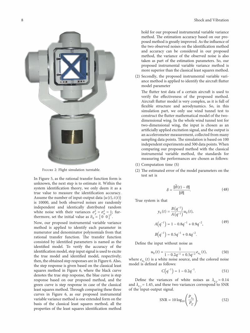

International Journal of
AerospaceEngineeringHindawiwwwhindawicom Volume 2018
RoboticsJournal of
Hindawiwwwhindawicom Volume 2018
Hindawiwwwhindawicom Volume 2018
Active and Passive Electronic Components
VLSI Design
Hindawiwwwhindawicom Volume 2018
Hindawiwwwhindawicom Volume 2018
Shock and Vibration
Hindawiwwwhindawicom Volume 2018
Civil EngineeringAdvances in
Acoustics and VibrationAdvances in
Hindawiwwwhindawicom Volume 2018
Hindawiwwwhindawicom Volume 2018
Electrical and Computer Engineering
Journal of
Advances inOptoElectronics
Hindawiwwwhindawicom
Volume 2018
Hindawi Publishing Corporation httpwwwhindawicom Volume 2013Hindawiwwwhindawicom
The Scientific World Journal
Volume 2018
Control Scienceand Engineering
Journal of
Hindawiwwwhindawicom Volume 2018
Hindawiwwwhindawicom
Journal ofEngineeringVolume 2018
SensorsJournal of
Hindawiwwwhindawicom Volume 2018
International Journal of
RotatingMachinery
Hindawiwwwhindawicom Volume 2018
Modelling ampSimulationin EngineeringHindawiwwwhindawicom Volume 2018
Hindawiwwwhindawicom Volume 2018
Chemical EngineeringInternational Journal of Antennas and
Propagation
International Journal of
Hindawiwwwhindawicom Volume 2018
Hindawiwwwhindawicom Volume 2018
Navigation and Observation
International Journal of
Hindawi
wwwhindawicom Volume 2018
Advances in
Multimedia
Submit your manuscripts atwwwhindawicom