Combining Bayesian Beliefs and Willingness to Bet to Analyze Attitudes

towards Uncertainty

by Peter P. Wakker, Econ. Dept.,Erasmus Univ. Rotterdam

(joint with Mohammed Abdellaoui & Aurélien Baillon) RUD, Tel Aviv, June 24 '07

Topic: Uncertainty/Ambiguity.

2

Making uncertainty/ambiguity more operational:

measuring, predicting,quantifying completely,in tractable manner.

No (new) maths; but "new" (mix of) concepts: uniform sources; source-dependent probability transformation.

1. Introduction

Good starting point for uncertainty: Risk.Many nonEU theories exist, virtually all amounting to:

x y 0; xpy w(p)U(x) + (1–w(p))U(y);

Relative to EU: one more graph …

3

4

inverse-S, (likelihood

insensitivity)

p

w

expected utility

mot

ivat

iona

l

cognitive

pessimism

extreme inverse-S ("fifty-fifty")

prevailing finding

pessimistic "fifty-fifty"

Abdellaoui (2000); Bleichrodt & Pinto (2000); Gonzalez & Wu 1999; Tversky & Fox, 1997.

Now to Uncertainty (unknown probabilities);

In general, on the x-axis we have events. So, no nice graphs …

5

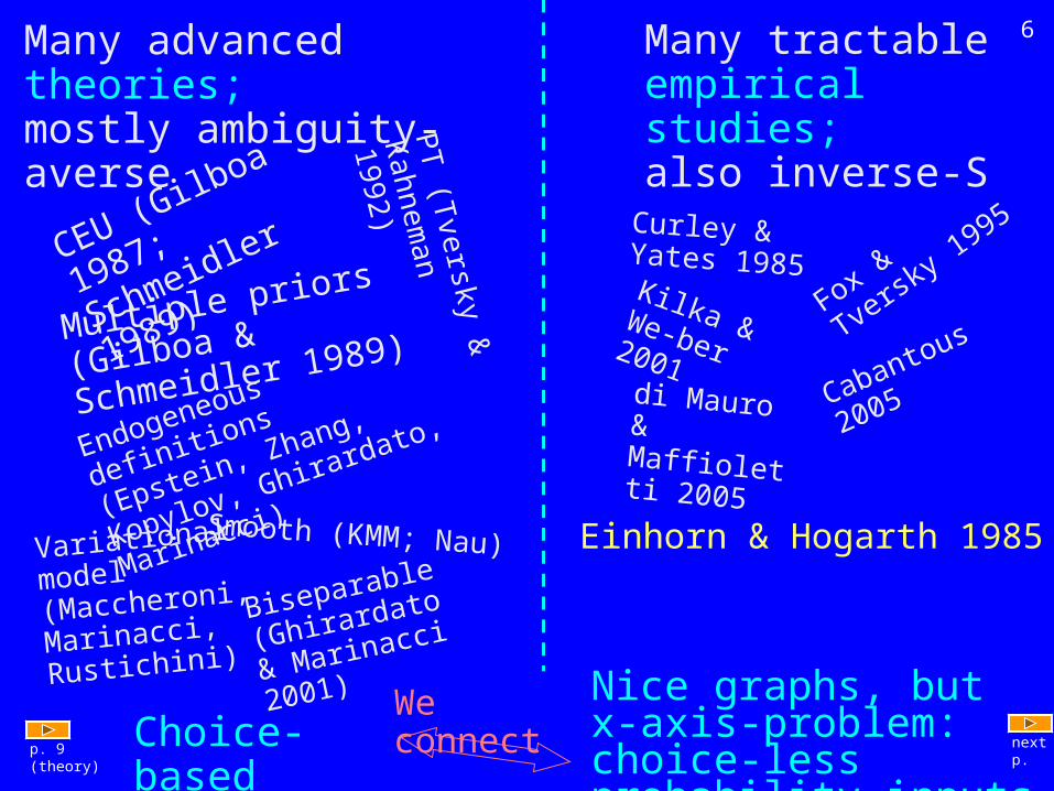
Many advanced theories;mostly ambiguity-averse

6

CEU (Gilboa 1987;

Schmeidler 1989)

PT

(Tversky &

Kahnem

an 1992)Multiple priors (Gilboa

& Schmeidler 1989)

Endogeneous definitions

(Epstein, Zhang, Kopylov,

Ghirardato, Marinacci)

Smooth (KMM; Nau)Variational

model (Maccheroni,

Marinacci,

Rustichini)

Many tractable empirical studies;also inverse-S

Curley & Yates 1985

Fox & Tve

rsky

1995

Biseparable

(Ghirardato &

Marinacci 2001)

Choice-based

Kilka & We-ber 2001

Cabantous

2005di Mauro & Maffioletti 2005

Nice graphs, but x-axis-problem: choice-less probability-inputs there

We connect

Einhorn & Hogarth 1985

next p.p. 9 (theory)

Einhorn & Hogarth 1985 (+ 1986 + 1990).Over 400 citations after '88.

For ambiguous event A, take "anchor probability" pA (c.f. Hansen & Sargent). Weight S(pA):

S(pA) = (1 – )pA + (1 – pA);

: index of inverse-S (regression to mean); ½.: index of elevation (pessimism/ambiguity aversion);

7

Einhorn & Hogarth 1985

Graphs: go to pdf file of Hogarth & Einhorn (1990, Management Science 36, p. 785/786).

Problem of the x-axis …

8

p. 6 (butter fly-theories)

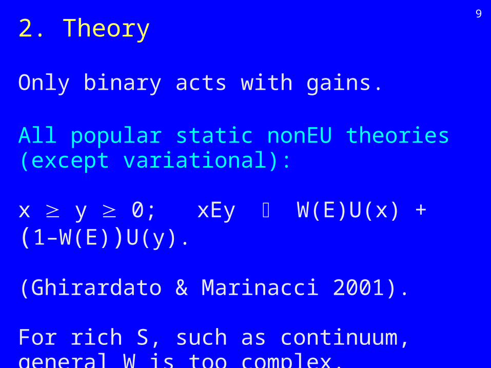
2. Theory

Only binary acts with gains.

All popular static nonEU theories (except variational):

x y 0; xEy W(E)U(x) + (1–W(E))U(y).

(Ghirardato & Marinacci 2001).

For rich S, such as continuum, general W is too complex.

9

Machina & Schmeidler (1992), probabilistic sophistication:

x y; xEy w(P(E))U(x) + (1–w(P(E)))U(y).

Then still can get nice x-axis for uncertainty!

However,

10

Common preferences between gambles for $100:(Rk: $100) (Ru: $100)(Bk: $100) (Bu: $100)

>

11

Ellsberg paradox. Two urns with 20 balls.

Ball drawn randomly from each. Events:Rk: Ball from known urn is red. Bk, Ru, Bu are similar.

Known urnk

10 R10 B

20 R&B in unknown proportion

Unknown urnu

? 20–?

P(Rk) > P(Ru) P(Bk) > P(Bk)

+1

+1 ><Under probabilistic sophistication

with a (non)expected utility model:

Ellsberg: There cannot exist probabilities in any sense. No "x-axis" and no nice graphs …

12

(Or so it seems?)

>

Common preferences between gambles for $100:(Rk: $100) (Ru: $100) (Bk: $100) (Bu: $100)

20 R&B in unknown proportion

Ellsberg paradox. Two urns with 20 balls.

Ball drawn randomly from each. Events:Rk: Ball from known urn is red. Bk, Ru, Bu are similar.

10 R10 B

Known urnk Unknown urnu

? 20–?

P(Rk) > P(Ru) P(Bk) > P(Bk)

+ +1 1 ><Under probabilistic sophistication

with a (non)expected utility model:

13

twomodels, depending on source

reconsidered.

Step 1 of our approach (to operationalize uncertainty/ambiguity):

Distinguish between different sources of uncertainty.

Step 2 of our approach:Define sources within which probabilistic sophistication holds. We call them

Uniform sources.

14

Step 3 of our approach:

Develop a method for (theory-free)* eliciting probabilities within uniform sources; empirical elaboration of Chew & Sagi's exchangeability.

* Important because we will use different decision theories for different sources

15

Step 4 of our approach:Decision theory for uniform sources S, source-dependent. E denotes event w.r.t. S.

x y; xEy wS(P(E))U(x) + (1–wS(P(E)))U(y).

wS: source-dependent probability transformation. (Einhorn & Hogarth 1985; Kilka & Weber 2001)

Ellsberg: wu(0.5) < wk(0.5) u: k: unknown known

(Choice-based) probabilities can be maintained.We get back our x-axis, and those nice graphs!

16

We have reconciled Ellsberg 2-color with Bayesian beliefs! (Also KMM/Nau did partly.)

We cannot do so always; Ellsberg 3-color(2 sources!?).

17

18

`c =0.08

w(p)

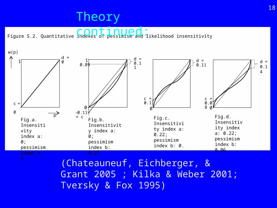
Fig.a. Insensitivity index a: 0;pessimism index b: 0.  

Figure 5.2. Quantitative indexes of pessimism and likelihood insensitivity

00.11= c

10.89

d =0.11

Fig.b. Insensitivity index a: 0;pessimism index b: 0.22. 

c =0.11

 

d =0.11

Fig.c. Insensitivity index a: 0.22;pessimism index b: 0.

0

d =0.14

Fig.d. Insensitivity index a: 0.22; pessimism index b: 0.06. 

d =01

p

c = 0 0

Theory continued:

(Chateauneuf, Eichberger, & Grant 2005 ; Kilka & Weber 2001; Tversky & Fox 1995)

3. Let the Rubber Meet the Road: An Experiment

Data:

19

4 sources:1. CAC40;2. Paris temperature;3. Foreign temperature;4. Risk.

Method for measuring choice-based probabilities20

EE EEE E

Figure 6.1. Decomposition of the universal event

a3/4

E

a1/2a1/4a1/8a3/8

E

b1a5/8 a7/8b0

a3/4a1/2a1/4

E E

b1b0

E E

a1/2

E

b1b0

E

E = S

b1b0

The italicized numbers and events in the bottom row were not elicited.

21

3025

Median choice-based probabilities (real incentives)

Real data over 19002006

0.035201510

0.8

0.6

0.4

0.2

1.0

Figure 7.2. Probability distributions for Paris temperature

Median choice-based probabilities (hypothetical choice)

0.0

Median choice-based probabilities (real incentives)

Real data over the year 2006

0 1 2 3123

0.8

0.6

0.4

0.2

1.0

Figure 7.1. Probability distributions for CAC40

Median choice-based probabilities (hypothetical choice)

Results for choice-based probabilities

Uniformity confirmed 5 out of 6 cases.

Certainty-equivalents of 50-50 prospects.Fit power utility with w(0.5) as extra unknown.

22

0

HypotheticalReal

1 2 30

1

0.5

Figure 7.3. Cumulative distribution of powers

Method for measuring utility

Results for utility

23

Results for uncertainty ("ambiguity?")

24

0.125

00

Figure 8.3. Probability transformations for participant 2

Fig. a. Raw data and linear interpolation.

0.25

0.875

0.75

1

0.50

0.125 0.8750.25 0.50 0.75 1

Paris temperature; a = 0.78, b =  0.12

foreign temperature; a = 0.75, b = 0.55

risk:a = 0.42, b = 0.13

Within-person comparisons

Many economists, erroneously, take this symmetric weighting fuction as unambiguous or ambiguity-neutral.

25

participant 2;a = 0.78, b = 0.69

0 *

Fig. a. Raw data and linear interpolation.

*

Figure 8.4. Probability transformations for Paris temperature

0.25

0.125

0.875

0.75

1

0.50

0.125 0.8750.250 0.50 0.75 1

participant 48;a = 0.21, b = 0.25

Between-person comparisons

Example of predictions [Homebias; Within-Person Comparison; subject lives in Paris]. Consider investments.Foreign-option: favorable foreign temperature: $40000unfavorable foreign temperature: $0Paris-option:favorable Paris temperature: $40000unfavorable Paris temperature: $0

Assume in both cases: favorable and unfavo-rable equally likely for subject 2; U(x) = x0.88. Under Bayesian EU we’d know all now.NonEU: need some more graphs; we have them!

26

27

Paris temperature Foreign temperature

decision weightexpectationcertainty equivalentuncertainty premiumrisk premiumambiguity premium

0.49 0.2020000 2000017783 6424

1357622175879 5879

7697–3662

Within-person comparisons (to me big novelty of Ellsberg):

28

Subject 2,p = 0.125

decision weightexpectationcertainty equivalentuncertainty premiumrisk premiumambiguity premium

0.35 0.675000 35000

12133159742732

571710257–3099

Subject 48,p = 0.125

Subject 2,p = 0.875

Subject 48,p = 0.875

5000 350000.08 0.52

2268

654 9663–39–4034

–71332078

962419026 25376

Between-person comparisons; Paris temperature

Conclusion:

By (1) recognizing importance of uniform sources and source-dependent probability transformations;(2) carrying out quantitative measurements of (a) probabilities (subjective), (b) utilities, (c) uncertainty attitudes (the graphs), all in empirically realistic and tractable manner,

we make ambiguity completely operational at a quantitative level.

29

The end

30