Combining Factor Models and External

Instruments to Identify Uncertainty Shocks

Martin Bruns∗

October 2018 - Job Market PaperMost recent version at this link

Abstract

Structural VAR models require two ingredients: (i) Informational suffi-

ciency, and (ii) a valid identification strategy. These conditions are unlikely to

be met by small-scale recursively identified VAR models which are commonly

used to explore the real and nominal effects of uncertainty shocks. I propose a

Bayesian Proxy Factor-Augmented VAR (BP-FAVAR) to jointly address both

issues. I find that real economic activity drops and rebounds following an iden-

tified uncertainty shock. The price reaction, while negative in the short run, is

indistinguishable from zero after six months. Informational insufficiency issues,

while detected by a statistical test, do not qualitatively alter these results.

JEL classification: C38, E60

Keywords: Dynamic factor models, external instruments, uncertainty shocks

∗Freie Universitat Berlin. German Institute for Economic Research (DIW Berlin). Email:mbruns@diw.de. I am grateful to Helmut Lutkepohl for excellent supervision. Lutz Kilian, HaroonMumtaz, Michele Piffer, and Barbara Rossi provided helpful suggestions.

1

1 Introduction

Following the seminal paper by Bloom (2009) a fast growing literature analyses the

macroeconomic impact of exogenous increases in uncertainty using structural VAR

models. An increase in uncertainty is broadly defined as increased difficulties of eco-

nomic agents to make accurate forecasts. Within this literature, there is a consensus

that exogenous increases in uncertainty lead to adverse real effects. These include

falling production, hours, and employment. However, there is an ongoing debate

about whether these reactions are dominated by supply or demand channels, i.e.

whether they are accompanied by a rise or fall in inflation. These nominal reactions

are crucial for policy makers: if, for example, central banks know that a rise in un-

certainty leads to a decrease in inflation, they can, theoretically, move both real and

nominal variables back to their desired targets by employing an expansionary policy.

If, on the other hand, uncertainty shocks do not affect prices or are inflationary, cen-

tral banks are faced with a trade-off between allowing for more inflation or a decline

in real activity.

In this paper, I propose a Bayesian Proxy Factor-augmented VAR (BP-FAVAR)

model to analyse the real and nominal effects following an uncertainty shock. This

novel model offers a unified framework to combine a large information set with a non-

recursive identification strategy. It addresses two shortcomings in commonly used

small-scale, recursively identified, VAR models: (i) informational insufficiency and

(ii) non-credible identification. I find that inflation responds negatively to a positive

uncertainty shock in the short run and is indistinguishable from zero after six months.

This is comforting news for policy makers given that they can address both real and

nominal effects using standard instruments. The dynamic effects depend strongly

on the identification scheme. Biases resulting from a recursive scheme cannot be

alleviated by augmenting the information set of the model.

The structural VAR literature is inconclusive about the inflationary effects of

uncertainty shocks. Leduc and Liu (2016), using a four-variable, recursively identified

VAR model, find that uncertainty shocks are deflationary, even in the medium term.

Piffer and Podstawski (forthcoming), identifying the work-horse model by Bloom

2

(2009) via an external instrument, find a short-lived drop and fast rebound in prices.

Caggiano, Castelnuovo and Nodari (2017), extending a small-scale VAR model to a

non-linear setting, find that uncertainty shocks are deflationary only in recessions and

have no effect on prices in expansions. Caggiano, Castelnuovo and Pellegrino (2017),

employing an interacted VAR model, find that the price reaction is indistinguishable

from zero over the whole impulse horizon.

At best, the theoretical literature provides limited guidance for the inflationary

effects of uncertainty shocks. Fernandez-Villaverde et al. (2015) and Born and Pfeifer

(2014) put forward two opposing channels to explain the potential price reaction fol-

lowing an exogenous increase in policy uncertainty: On the one hand, if consumers

face difficulties predicting the next period, they will postpone consumption decisions,

which will lead to a fall in both economic activity and prices. Therefore, an uncer-

tainty shock would resemble an aggregate demand shock. Using a model with labour

market frictions, Leduc and Liu (2016) also reach this conclusion. On the other hand,

if firms face difficulties predicting the next period, they will bias their price decision

upwards. The reason is that their profit function is concave in prices, making it

more costly to set prices too low rather than too high. If this “price-bias-channel”

dominates, the reactions of real and nominal variables will resemble a short-lived

aggregate supply shock. The aggregate reaction of prices from these two opposing

channels is ambiguous.

The responses to an uncertainty shock may depend heavily on the information

set of the model, as pointed out by Caggiano, Castelnuovo and Nodari (2017) and

Angelini et al. (2018). In particular, omitted variables, such as consumer sentiment

(Sims, 2012), total factor productivity (Bachmann and Bayer, 2013), and measures

of anticipated risk (Christiano et al., 2014) may bias the impulse responses. In or-

der to avoid having to add potentially omitted variables one by one, I augment the

work-horse VAR model by Bloom (2009) with latent factors. These summarise the

information contained in a large set of variables and, thus, should alleviate omitted

variable biases. Second, as pointed out by Stock and Watson (2012), a recursive iden-

tification scheme may be invalid given the contemporaneous interrelation between the

real economy and uncertainty as well as the fast moving nature of financial markets.

3

Therefore, a recent strand of the literature addresses identification issues by depart-

ing from recursive schemes and employing external instruments. I follow Piffer and

Podstawski (forthcoming) in identifying an uncertainty shock using a proxy based

on the price of gold. This proxy captures movements in the price of gold around se-

lected economic and political events. These events are associated with movements in

uncertainty. Given that gold can be considered a safe haven asset, these movements

should capture exogenous variations in uncertainty.

Estimation of the model is subject to two challenges. The first regards the so-

called ”curse of dimensionality”. Even after shrinking the variable space using latent

factors, the model still contains a large number of parameters. The baseline model

consists of over 800 parameters, while the effective sample length is only roughly

400. Therefore, estimation is infeasible in a frequentist setting. A second challenge

arises from the need to effectively summarise the estimation uncertainty in both the

model parameters and the latent factors. This is difficult using bootstrap techniques

(see for example Yamamoto, forthcoming). In addition, there are no asymptotic

results justifying the use of such techniques, as pointed out by Kilian and Lutkepohl

(2017). To jointly address these two challenges I employ a Bayesian approach. It

allows for overcoming dimensionality problems by shrinking the parameter space

and summarises the estimation uncertainty in a joint posterior distribution. The

BP-FAVAR can be considered a combination of the Bayesian FAVAR estimation

proposed by Belviso and Milani (2006) and the Bayesian Proxy VAR by Caldara

and Herbst (forthcoming). I re-parametrize their model to impose structure on the

impact effects of shocks.

The main results are the following: Uncertainty shocks are deflationary in the

short run. The price reaction is indistinguishable from zero after about six months.

Real variables and the stock market drop and rebound. This suggests that policy

makers can employ an expansionary policy to alleviate the adverse effects of an ex-

ogenous increase of uncertainty on both prices and real activity. I show evidence that

the workhorse model by Bloom (2009) is informationally deficient. When computing

impulse responses, I find that alleviating informational deficiency problems has only

marginal quantitative effects. This finding is in line with Sims (2012), who points

4

out that informational deficiency is not an either/or but a quantitative issue. In the

present case the biases it causes are negligible, which is comforting news.

The remainder of the paper is organized as follows: Section 2 introduces the

model setup and explains the identification of uncertainty shocks. Section 3 presents

the data and discusses the results. The last section concludes.

2 The Bayesian Proxy FAVAR

In this section, I introduce the Bayesian Proxy FAVAR model. I start by describ-

ing the different parts of the model. Then, I discuss how partial identification is

achieved. Last, I show how the model can be decomposed into three blocks to facil-

itate inference.

2.1 Model Description

The Bayesian Proxy Factor-augmented VAR model admits a state-space form, which

consists of an observation equation, a transition equation and a proxy equation.

First, consider the observation equation, which shows how latent and observable

factors map into informational series:

xt = Λff t + Λzzt + ξt (1)

ξt ∼ N(0,Ω) (2)

where xt is a N × 1 vector of observable series, f t is a R× 1 vector of latent factors,

and zt is a K × 1 vector of observable factors. Importantly, xt does not contain

any of the observable factors in zt. Λf is a N × R matrix of factor loadings for

latent factors and Λz is a N × K matrix of coefficients for the observable factors.

ξt is a N × 1 vector of idiosyncratic errors. In general, ξt can be serially correlated,

i.e. Cov(ξt, ξt−1) 6= 0, but they are uncorrelated across series, i.e. V ar(ξt) = Ω is

assumed to be diagonal.

Next, consider the transition equation which shows the dynamic evolution of the

5

factors. It writes as a VAR(P) of the following form:

yt = Πwt + ut (3)

ut ∼ N(0,Σ), (4)

where yt =

[f t

zt

]stacks latent and observable factors in a vector. The coefficient

matrix Π = [Π1, ...,ΠP ] of dimension R + K × (P (R + K) + 1) contains the au-

toregressive parameters of the VAR. wt = [1R+K×1;yt−1, ...,yt−P ] stacks a constant

and P lags of yt. The (R + K) × 1 vector of reduced form errors, ut, is serially

uncorrelated, i.e. Cov(ut,ut−p) = 0 ∀t = 1, ..., T , ∀p = 1, ...,∞. Also, ut are un-

correlated with all leads and lags of the idiosyncratic errors, ξt, i.e. Cov(utξt−j) = 0

∀j, ∀t = 1, ..., T .

I impose structure on the on-impact effects of structural shocks by assuming that

the reduced form errors map into structural shocks as:

ut = Bεt (5)

εt ∼ N(0, IR+K), (6)

where B is a (R + K) × (R + K) matrix containing the on-impact effects of the

structural shocks. Their variance is normalised to one and they are contemporane-

ously uncorrelated. This implies the following relation between the reduced form

covariance matrix and the matrix of on-impact effects: Σ = BB′

As is well known, further restrictions beyond those implied by the covariance

matrix are needed to identify B. The reason is that the data cannot discriminate

between observationally equivalent representations: All B such that BB′ = Σ yield

the same likelihood. Therefore, without imposing further structure, the econometri-

cian cannot distinguish between B and B = BQ, where Q is an orthogonal matrix

such that QQ′ = I.

In order to identify the first column of B, which I denote b, I augment the model

by a ”Proxy Equation”, as in Caldara and Herbst (forthcoming). It spells out the

6

relation between structural shock and instrument and is given as1:

mt = βε1,t + σννt (7)

νt ∼ N(0, 1), (8)

where mt is a scalar instrument correlated with the shock of interest, ε1,t. The shock

of interest is ordered first, without loss of generality. Furthermore, mt is orthogonal

to all other shocks, ε−1,t, i.e. E(mtε−1,t) = 0 ∀t, where ε−1,t stands for a vector

containing all but the first shock. In other words, the instrument needs to be both

relevant and exogenous in order to be appropriate for identification. β captures the

structural relationship between instrument and shock, while νt captures any noise

contained in the instrument. The higher its variance, σ2νs, the less information the

instrument contains about the shock of interest.

The full model can be written in compact matrix notation as:xtztmt

=

Λf Λz 0N×1

0K×R IK 0K×1

01×R 01×K 1

f tztmt

+

ξt

0K×1

0

(9)

V ar([ξt

]) = Ω (10)[

yt

mt

]=

[Π(L)

01×P (K+R)

]wt + B

[εt

νt

](11)

V ar(

[εt

νt

]) =

[IR+K 0R+K×1

01×R+K 1

], (12)

1Unlike their case, however, identification focuses on the on-impact effects of the shocks ratherthan on the contemporaneous relations of the variables included in the model. Put differently, themodel imposes structure on B, rather than on B−1. Caldara and Herbst (forthcoming) estimate aso-called A-model (see Kilian and Lutkepohl, 2017 for a discussion). The A-model specification isappropriate given their aim of identifying a monetary policy equation. In the context of uncertaintyshocks, however, it is more common to inform the on-impact effects of shocks (see e.g. Bloom, 2009or Caggiano, Castelnuovo and Nodari, 2017). Therefore, I propose to use a so-called B-model,which imposes structure on the on-impact effects.

7

where B =

[B β

β′ σν

], and β =

[β

0R+K−1×1

].

2.2 Identification

Shock identification in the BP-FAVAR model is achieved by weighting draws from the

posterior of structural parameters. In particular, more weight is given to posterior

draws which lead to a close relation between instrument and the shock of interest.

To be more precise, consider the joint likelihood of xt, yt and mt given a draw of

the latent factors2:

p(X,Y ,m|Π,Σ,Λf ,Λz,Ω, β, σν , b) (13)

=p(Y |Π,Σ,Λf ,Λz,Ω)

· (m|Y ,Π,Σ,Λf ,Λz,Ω, β, σν , b)

· (X|m,Y ,Π,Σ,Λf ,Λz,Ω)

where X = [x1, ...,xT ], Y = [y1, ...,yT ] and m = [m1, ...,mT ] stack the obser-

vational series, the factors, and the instrument horizontally. Note that, while the

marginal likelihood of Y and the conditional likelihood of X|m,Y depend only on

reduced form parameters, the conditional likelihood of m|Y depends, in addition,

on structural parameters, β, σν and b.

The conditional likelihood of m|Y can be written as (see Appendix for deriva-

2The factors are identified only up to an invertible rotation, i.e. the representations xt = Λyt+ξtand xt = ΛPP−1yt + ξt yield the same likelihood. Therefore, in order to achieve identification,one has to impose further restrictions. I follow Bernanke et al. (2005) and set the upper R × Kblock of Λz equal to a zero matrix. Furthermore, Σf = Cov(f t) is diagonal and Λf′

Λf

N = IR. Thisnormalisation, although not necessary, is sufficient to pin down the factor rotation, as pointed outby Kilian and Lutkepohl (2017).

8

tion):

m|Y ∼ N(µm|Y ,V m|Y ) (14)

µm|Y = βε1 (15)

V m|Y = σ2νIT , (16)

where ε1 = [ε1,1, ..., ε1,T ] stacks the structural shocks of interest in a vector.

As seen in equation (15), the conditional likelihood of m is higher the closer

are m and βε1. In the posterior sampler, draws are weighted by the conditional

likelihood of m (see Appendix C). Therefore, the econometrician will give more

weight to posterior draws, which result in structural errors that look like a scaled

version of the proxy.

As is apparent from equation (15), since ε1 is obtained from reduced form errors,

identification depends heavily on the model specification. Therefore, one should pay

close attention to which variables are included in the model since an omitted variable

bias translates into biases in the identified structural shocks. Augmenting the model

with latent factors helps alleviate this problem without taking a stand on which of

a potentially large set of observational series need to be included.

Compared to recursively identified VARs, the BP-FAVAR has the advantage that

when using a Proxy VAR, the researcher is not forced to employ potentially non-

credible short run exclusion restrictions. For example, the recursive workhorse model

on the empirical identification of uncertainty shocks by Bloom (2009) relies on the

assumption that financial markets do not price an exogenous increase in uncertainty

within a month. This might be too strong an assumption given the fast-moving

nature of financial markets. In the context of Proxy VAR models such short run

exclusion restrictions are substituted by external information contained in the proxy

variable, mt.

9

2.3 Inference

The Bayesian approach treats all model parameters and latent factors as random

variables whose posterior needs to be sampled from. In order to outline the sampling

procedure, first define the parameter space as

θ = (Π,Σ,Λf ,Λz,Ω, β, σν , b) (17)

The joint posterior of parameters and latent factors is:

p(θ,F |X,Z,m), (18)

where F = [f 1, ...,fT ], Z = [z1, ...,zT ]. The challenge consists in approximating

the marginal posterior distributions of the latent factors,

p(F |X,Z,m) =

∫θ

p(θ,F |X,Z,m)dθ (19)

and the model parameters,

p(θ|X,Z,m) =

∫F

p(θ,F |X,Z,m)dF (20)

It is shown by Geman and Geman (1984) that these integrals can be approximated

using a multi-move Gibbs sampler, which alternately draws from two distributions:

First, draw the latent factors given all model parameters and the data, i.e.

p(F |θ,X,Z,m). (21)

10

This draw is generated using filtering techniques. Second, draw the model parameters

conditioning on this draw of factors and the data, i.e.3

p(θ|Z,X,m). (22)

This draw is generated using a Metropolis-within-Gibbs algorithm as in Caldara and

Herbst (forthcoming).

Compared to the common approach of first extracting factors via Principal Com-

ponents and then feeding them into a VAR (see Stock and Watson, 2016 for a review),

this Bayesian approach has the advantage that it allows for Bayesian shrinkage of the

parameter space. This might seem unnecessary given that the factors already reduce

the dimensionality of the estimation problem. However, if, as in the present case,

the number of observable factors, K, or the lag length, P , is large, dimensionality

issues still arise and can be alleviated using Bayesian shrinkage.4 Furthermore, as

shown by Yamamoto (forthcoming), bootstrap inference in frequentist factor models

is far from trivial. In particular, it remains an open issue how to account for the

estimation uncertainty in the factors. A Bayesian approach, on the other hand, offers

a unified way of summarising the uncertainty of the model, as pointed out by Huber

and Fischer (2018). The joint posterior summarises estimation uncertainty in both

the parameters and the latent factors.

Conditional posterior densities of latent factors F given θ: The procedure

to generate posterior draws of latent factors, F , differs from generating draws of

parameters, θ, in that one has to generate the whole dynamic evolution of factors for

each t = 1, ..., T . For this to be feasible I exploit the Markov property of the system

3I follow Caldara and Herbst (forthcoming) and generate draws from p(F |θ,X) and p(θ|Z,X)first and account for the additional conditioning on m using an independence Metropolis-Hastingsstep. See Appendix C for details.

4The number of parameters to be estimated in the transition equation is

(R+K)(1 + (R+K)P ) + (R+K)2

=(4 + 8)(1 + (4 + 8)5) + (4 + 8)(4 + 8 + 1)/2

=810.

The sample length is T = 438.

11

described in equation (3) as follows:

p(Y |X,θ) = p(yt|X,θ)T−1∏t=1

p(yt|yt+1,X,θ). (23)

First note that (23) describes the posterior of Y , which contains both latent and

observable factors. The reason for including the observable factors is the dynamic

interdependence between latent and observable factors, which needs to be accounted

for. Given that the observable factors are non-random, their distribution has a zero

variance.5 Second, note that this is a product of R+K-dimensional conditional dis-

tributions. Given the assumption of Gaussianity of ξt and ut, this representation can

be combined with the observation equation (1) and is amenable to the Carter-Kohn

algorithm described in Carter and Kohn (1994) and Fruhwirth-Schnatter (1994) (see

Appendix E for details). This approach, while straightforward to implement, in-

creases the computational burden slightly compared to Principal Components Anal-

ysis. However, it allows incorporating the estimation uncertainty in the latent factors

in a consistent way.

Conditional posterior densities of the parameters θ given latent factors

F : In order to draw the model parameters θ given the data and a draw of the factors,

Y , I form three blocks of parameters: Block 1 refers to parameters of the observation

equation (1), block 2 refers to the parameters of the transition equation (3), and block

3 refers to the parameters of the proxy equation (7). Conditional on a draw of the

factors and the data the first two blocks can be sampled independently of each other

while the last block is sampled conditional on the second block.

Block 1: Observation Equation The idiosyncratic errors ξt are assumed to be

mutually uncorrelated and normally distributed. Group the factor loading matrices

as Λ = [Λf Λz]. Then, conditional on a draw of the factors, we can specify con-

jugate normal-inverse Gamma priors and draw the posterior for Λ and Ω equation-

by-equation using well-known results on Bayesian linear regression models (see e.g.

5Here, I refer to the variance across draws. The variance across time is, of course, non-zero.

12

Koop, 2003). For each equation i, specify the priors as:

ωii ∼ IG(sc∗, sh∗) (24)

λi|ωii ∼ N(µ∗λ,i,ωiiM∗−1i ), (25)

where λi is the i-th row of Λ and ωii is the i-th diagonal element of Ω. These priors

translate into posterior distributions of the following form:

ωii|X,Y ∼ IG(sci, shi) (26)

λi|ωii,X,Y ∼ N(µλ,i,ωiiM−1i ) (27)

with

shi = sh∗ + T (28)

sci = sc∗ + ξiξi′+ (λ

OLS

i − µ∗λ,i)′(M−1i + (Y Y ′)−1)−1(λ

OLS

i − µ∗λ,i) (29)

λOLS

i = xiY′(Y Y ′)−1 (30)

ξi = xi − λOLS

i Y (31)

M i = M ∗i + Y Y ′ (32)

µλ,i = M i(M∗−1i µ∗λ,i + Y Y ′λ

OLS

i ) (33)

I follow Bernanke et al. (2005) in specifying sc∗ = 3, sh∗ = 10−3, M ∗i = IR+K and

µ∗λ,i = 0(R+K)×1.

Block 2: Transition Equation Given a draw of factors, yt follows a standard

V AR(P ) model. Therefore, we can employ a version of the Minnesota/ Litterman

prior and specify independent normal-inverse Wishart priors:

vec(Π) ∼ N(µ∗Π,V∗Π) (34)

Σ ∼ IW (S∗, τ ∗), (35)

where vec(·) is the vectorisation operator that stacks the column of a matrix one un-

13

derneath the other into a vector. These priors translate into the following conditional

posterior for vec(Π):

vec(Π)|Σ,Y ∼ N(µΠ, V Π) (36)

V Π = (V ∗−1Π + (WW ′ ⊗Σ−1))−1 (37)

µΠ = V Π(V ∗−1Π µ∗Π + (W ⊗Σ−1)vec(Y )) (38)

where W = [w1, ...,wT ], wt = [1 yt−1 ... yt−p]′ stacks a vector of 1s and P lags

of yt. The conditional posterior for Σ is given as:

Σ|Π,Y ∼ IW (S, τ) (39)

S = S∗ +UU ′ (40)

τ = τ ∗ + T, (41)

where U = [u1, ...,uT ] stacks the reduced form errors given the current draw of

factors. I set µ∗Π to a zero vector given that all series are transformed to be stationary.

V ∗Π is a diagonal matrix containing the prior variances of the parameters contained

in Π. These are set in accordance with standard Minnesota values and given as:

v∗Π,i,j =

(λ/l)2 if i = j

(λσi/lσj)2 if i 6= j,

(42)

where σi is obtained from univariate AR(1) regressions and λ = 0.2. S∗ is set to

IR+K , while τ ∗ is set to R +K.

Block 3: Proxy Equation The parameters of the proxy equation are sampled

conditional on the parameters of the transition equation. For β and σν the priors

are

β ∼ N(µ∗β, σ∗β) (43)

σν ∼ IG(sc∗ν , sh∗ν). (44)

14

b is computed as b = chol(Σ)Q·,1 where Q·,1 is the first column of a draw from the

uniform Haar distribution (see Rubio-Ramirez et al., 2010 for a discussion).

These priors translate into the following posteriors for β and σν :

β|Y ,m,Π,Σ, σν , b ∼ N(µβ, σβ) (45)

µβ = mε1(ε1ε1′)−1 (46)

σβ = σν(ε1ε1′)−1 (47)

σν |Y ,m,Π,Σ, β, b ∼ IG(scν , shν) (48)

scν = sc∗ν + (m− βε1)(m− βε1)′ (49)

shν = sh∗ν + T (50)

For b the conditional posterior has an unknown form. Therefore, b is sampled using a

Metropolis-Hastings step. In particular, at iteration j, a draw bcand, will be accepted

with probability (see Appendix C for details)

α = min(p(m|Y ,Π,Σ, bcand)

p(m|Y ,Π,Σ, bj−1), 1) (51)

I follow Caldara and Herbst (forthcoming) in specifying the priors as µ∗β = 0, σ∗β = 1,

sh∗ν = 2, sc∗ν = 0.2 in order to allow the data to dominate the posterior. In particular,

this prior specification implies a zero mean prior correlation between instrument and

shock, ρ.

Posterior Sampler The sampler can be summarized as follows (see the Ap-

pendix C for a detailed step-by-step procedure):

1. Set starting values

2. Draw yt via the Carter-Kohn algorithm

3. Draw Λ and Ω

4. Draw Σ and Π

15

5. Draw b using a Metropolis-Hastings step

6. Draw β and σν

These steps are repeated a sufficient number of times for the algorithm to converge

(see Appendix E.3 for a discussion of the convergence properties of the sampler).

3 Data, Estimation and Results

This section first describes the data and the proxy used for identification. It then

shows how the number of factors is determined with the goal of alleviating informa-

tional insufficiency issues. Lastly, it discusses how instrument relevance is assessed

in the Bayesian context and presents impulse responses from the baseline model as

well as from three benchmark models.

3.1 Data and Transformations

The baseline data contained in zt are monthly US data from Piffer and Podstawski

(forthcoming), who updated the data in Bloom (2009). The vector of observational

series, xt, contains 126 of the monthly FRED dataset by McCracken and Ng (2016)

that are not already included in zt (see Appendix F for a detailed description).6 The

length of the estimation sample is constrained by the instrument7 and lasts from

1979M1 through 2015M7.8 I follow Piffer and Podstawski (forthcoming) in setting

the lag length to P = 5 as a baseline (see Appendix A for a robustness exercise

setting P = 9).

One concern is measurement of the monetary policy stance. Traditionally, the

effective federal funds rate is considered to be the policy tool of the central bank.

However, given that it was constrained by the zero lower bound in the period 2009M1

6Data set available at https://research.stlouisfed.org/econ/mccracken/fred-databases/7Instrument available at https://sites.google.com/site/michelepiffereconomics/home/research-18An alternative to shortening the sample is put forward by Braun et al. (2017). They suggest

generating synthetic observations for the instrument within their posterior sampler. This procedureimplicitly requires parameter stability for time periods when the instrument is unavailable and itassumes that missing values occur at random.

16

to 2015M11, this variable cannot serve as an indicator of the policy stance. This is

why, for this period, I replace the effective federal funds rate by the shadow rate as

computed by Wu and Xia (2016). It is based on a term structure model and often

considered a better reflection of the policy stance during the zero lower bound period

than the federal funds rate. Figure 16 in Appendix F shows the shadow rate.

All informational series contained in xt are transformed to have zero mean. In

addition, they are transformed to induce stationarity as proposed by McCracken and

Ng (2016). Missing values are replaced with zeros, which is the unconditional mean

of the standardized series. These missing values occur mostly at the beginning of

the dataset and amount to less than one percent of total observations. Therefore,

the joint dynamics are unlikely to be overly affected by this imputation.

Piffer and Podstawski (forthcoming) argue that a proxy for the uncertainty shock

could be based on the price of gold. The intuition behind this idea is that gold is

considered a safe haven asset that investors choose in times of heightened uncertainty.

This generates movements in the price of gold. The challenge consists in finding price

variations that are not correlated with structural shocks other than the uncertainty

shock (exogeneity condition). In order to achieve this, the authors collect a series of

38 events, which are considered to be associated with movements in uncertainty (e.g.

the fall of the Berlin Wall or the 9/11 terrorist attacks). They then compute the

variation of the gold price in narrow windows around these events and argue that

these variations are driven exclusively by movements in uncertainty. In addition,

they show that this proxy has a low correlation with other structural shocks as

computed by Stock and Watson (2012), which is further evidence for exogeneity to

their system.

Figure 1 shows the proxy. It peaks during well-known events such as the 9/11

terrorist attacks in 2001 or the bankruptcy of Lehman brothers in 2008.

3.2 Determining the Number of Factors

Choosing the number of latent factors, R, has important consequences for the amount

of additional information the BP-FAVAR is based on, compared to the small-scale

17

1980 1985 1990 1995 2000 2005 2010 2015

-0.04

-0.02

0

0.02

0.04

0.06

Gold Price Proxy

Figure 1: Uncertainty Proxy. Gold price variation around selected events. The sample period

is 1979M1 to 2015M7.

VAR model employed in Bloom (2009) and Piffer and Podstawski (forthcoming).

Stock and Watson (2016) stress the importance of using different statistical esti-

mators to determine R. I employ two complementary tools: A scree plot and a

sequential testing procedure, as proposed by Forni and Gambetti (2014). The choice

of these two criteria is driven by the main purpose of the factors, which is to align

the econometrician’s and the economic agent’s information sets.

A scree plot summarizes the marginal contribution of the r-th factor to the aver-

age explanatory power of N regressions of xt against the first r factors as computed

via Principal Components. Figure 2 plots this marginal contribution against the

number of factors. It shows that the first factor explains about 60% of variance in

xt, while the first four factors explain over 95% of the variance.

The sequential testing procedure chooses the number of factors R so as to ensure

that the resulting BP-FAVAR model aligns the econometrician’s and the agent’s

information set. This would not be the case in the presence of omitted variables.

18

1 2 3 4 5 6 7 8 9 10

R

0

0.1

0.2

0.3

0.4

0.5

Exp

lain

ed V

aria

nce

Figure 2: Scree Plot. Explained share of variance in xt as a function of the number of latent

factors (R) included in f t

This procedure is particularly suited when the list of potentially omitted variables

is large and the researcher therefore would like to avoid taking a stand on which

additional variables to include. In the context of uncertainty shocks, variables which

are typically omitted from small-scale VAR models but could potentially be relevant,

include consumer sentiment (Bachmann and Sims, 2012), total factor productivity

(Bachmann and Bayer, 2013), and measures of anticipated risk (Christiano et al.,

2014). Other forward-looking variables could also potentially cause omitted variable

biases.

Instead of including one variable after the other in the VAR the sequential testing

procedure augments the small-scale VAR model by latent factors extracted from a

large set of informational series until the model is informationally sufficient. The

model is informationally sufficient if none of the observable variables is Granger-

caused by factors. The basis is a multivariate out-of-sample Granger-causality test

(see Appendix D for details). The intuition behind this test is the following: If the

19

economy is accurately represented by a factor model, as is assumed here, then the

factors contain all relevant information that agents base their decision making on. If

these factors do not help predict a vector of variables in the VAR, then the variables

in the VAR contain the same information as the factors. Thus, they are sufficient to

align the econometrician’s and the agent’s information set. If, on the other hand, the

factors do help predict the VAR variables, then they should be subsequently added

to the VAR as additional variables until informational sufficiency cannot be rejected

any longer. The sequential testing procedure is as follows:

In a first step, I test

H0 : fPCt do not Granger-cause zt (52)

H1 : fPCt Granger-cause zt, (53)

where fPCt is a vector containing the first six Principal Components extracted from

xt. I then test, for j = 1, ..., 5

H0 : fPCt,−(1:j) do not Granger-cause zt,f t,1:j (54)

H1 : fPCt,−(1:j) Granger-cause zt,f t,1:j. (55)

where fPCt,1:j are the first j Principal Components of xt and fPCt,−(1:j) is a vector con-

taining all but the first j Principal Components.

Figure 3 shows the distribution of the test statistic across 1000 samples obtained

via a standard residual bootstrap procedure together with the test statistic computed

using the actual sample data. If the actual test statistic lies outside the bootstrap

distribution test statistic, then this indicates that the Null of no Granger causality

can be rejected.

Table 1 shows the corresponding p-values. It suggests that for R = 0, informa-

tional sufficiency can be rejected. This can be considered evidence that the workhorse

model of Bloom (2009) is, indeed, informationally deficient and needs to be extended

in order to alleviate potential omitted variables biases. The Null Hypothesis of in-

formational sufficiency cannot be rejected once the model is augmented by at least

20

R=0

-0.5 0 0.5 10

0.1

0.2R=1

-0.5 0 0.5 10

0.1

0.2

R=2

-0.5 0 0.5 10

0.2

0.4R=3

-0.5 0 0.5 10

0.2

0.4

R=4

-0.5 0 0.50

0.2

0.4

distr(H0)test stat

R=5

-0.4 -0.2 0 0.2 0.40

0.2

0.4

Figure 3: Test for Informational Sufficiency. The histogram shows the bootstrap test statistic

under the Null of no Granger-causality. It is based on a multivariate one-step-ahead out-of-sample

Granger-causality test with lag length 4. The bootstrap test statistic is based on 1000 replications.

The sample is split as T = T1 + T2, T1 = T2 = 0.5T . A larger test statistic indicates Granger-

causality. Rejection of the Null of no Granger-causality indicates informational deficiency.

four factors. Therefore, the multiple testing procedure suggests using R = 4.

Combining the information from the scree plot and the sequential testing proce-

dure, I choose to set R = 4.

Figure 4 shows the last accepted draw of estimated factors from the Bayesian

estimation, together with the Principal Components estimation used as a starting

value. The two estimation procedures yield similar results suggesting that Principal

Components can be used as an approximation to determine R.

3.3 Relevance of the Instrument

The instrument is appropriate to identify the uncertainty shock to the extent that it

contains enough information about the shock, i.e. it is relevant. The relevance of the

21

R p-value

0 0.00001 0.00202 0.00003 0.00004 0.12405 0.6680

Table 1: Test for Informational Sufficiency. p-values are obtained as the fraction of bootstrap

test statistics under the Null of no Granger causality exceeding the actual test statistic.

1980 1990 2000 2010

-2

0

2

4

Factor 1

1980 1990 2000 2010-6

-4

-2

0

2

4Factor 2

1980 1990 2000 2010

-2

0

2

4

Factor 3

1980 1990 2000 2010

-4

-2

0

2

Factor 4

Bayesian EstimationPC estimation

Figure 4: Factors Last accepted draw from posterior sampler and Principal Components estima-

tion of factors

22

β

-0.2 -0.15 -0.1 -0.05 0 0.05 0.1 0.15 0.20

2

4

6

8

10

12 prior

posterior

σν

0.05 0.1 0.15 0.2 0.25 0.30

5

10

15

20

25

30

35

40

45

50 prior

posterior

ρ

-1 -0.8 -0.6 -0.4 -0.2 0 0.2 0.4 0.6 0.8 10

0.5

1

1.5

2

2.5

prior / prior

post/ post

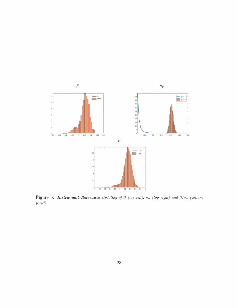
Figure 5: Instrument Relevance Updating of β (top left), σν (top right) and β/σν (bottom

panel)

23

instrument in the Bayesian context is assessed by analysing the posterior updating

of the proxy equation. A high posterior correlation between instrument and shock

suggests relevance.

Figure 5 shows the updating of the relevant quantities β, σν and their ratio

β/σν . This ration is the signal-to-noise ratio and measure how much information the

instrument contains about the shock of interest.

The top left panel shows that while using a prior for β that is flat over the

relevant parameter space, the posterior is centred around 0.1 suggesting that the

data support a structural relationship between structural error ε1,t and instrument

mt. The top right panel shows the updating of σν . The prior is chosen to have mean

0.02 and infinite variance. The posterior suggests a standard deviation of this noise

measurement centred around 0.2. The bottom panel shows what this implies for the

signal-to-noise ratio. While the prior is centred around zero and flat over the whole

parameter space, the posterior is centred around 0.15 and has little probability mass

near zero. This strongly suggests that the instrument contains relevant information

about the structural shock.

3.4 Updating of b

Given that both the recursive identification scheme and the proxy identification

scheme impose structure on the impact effect of shocks, differences between these two

approaches will be most apparent in the identification of b. It contains the impact

effects of the uncertainty shocks on the latent and observable factors. The prior

distribution is not available in closed form but is implicit in the prior distributions

of Σ, Q·,1, β and σν . Prior draws are generated imposing the prior mean for β, i.e.

setting β = 0, so that all rotation vectors, Q·,1, are accepted with equal probability.

A draw from the prior of b is computed as follows:

• Draw Σprior from its prior inverse Wishart distribution

• Draw Qprior·,1 as the first column of a draw from the uniform Haar distribution

• Compute bprior = chol(Σ)Q·,1.

24

-0.5 0 0.50

2

4

Fac

tor

1

-0.2 0 0.20

5

10

Fac

tor

2

-0.4 0 0.40

2

Fac

tor

3

-0.4 -0.2 0 0.20

2

4

Fac

tor

4

-2 0 20

0.5

S&

P 5

00

-1 0 1 2 30

0.5

VX

O

-0.2 0 0.20

2

4

Fed

fund

s ra

te

-0.1 0 0.10

5

Wag

e

-0.1 0 0.10

5C

PI

-0.1 0 0.10

5

10

Hou

rs

-0.1 0 0.10

5

10

Em

ploy

men

t

-0.4 0 0.40

2

Ind.

Pro

duct

ion

Figure 6: Update of b: Updating of the first column of B (not normalised). The blue line shows

the prior distribution of b computed as the distribution implicit in the priors on Σ and Q·,1 and

plotted using a Kernel smoother. The bars show the posterior.

25

As pointed out by Baumeister and Hamilton (2015), a uniform prior on Q·,1 does not

necessarily imply a uniform distribution over the structural parameters of interest,

which in this case are the elements of b. Figure 6 shows that, indeed, the implicit prior

on b has some curvature on the impact effect of the S&P 500 index and the VXO.

However, it has good coverage of the relevant parameter space. More importantly,

it is flat in the relevant parameter regions for the variables of prime interest, namely

CPI, hours, employment, and industrial production as well as the latent factors.

Therefore, the implicit prior on b should not overly affect the posterior of b.

3.5 Impulse Responses

The BP-FAVAR extends the workhorse model by Bloom (2009) in two ways: First,

instead of imposing exclusion restrictions on b, the BP-FAVAR achieves identification

via a proxy. Second, the BP-FAVAR addresses informational deficiency of the Bloom

(2009) model, which could potentially bias the responses of variables to the uncer-

tainty shock. The workhorse model contains the following variables: ∆log(S&P500),

VXO, federal funds rate, ∆log(wages), ∆log(CPI), hours, ∆log(employment), and

∆log(IP ). In order to isolate the effects of the identification scheme and the informa-

tion set, I include three benchmark models to compare to the baseline BP-FAVAR:

BP-VAR. This model can be considered a Bayesian adaptation of the model by

Piffer and Podstawski (forthcoming). I use their model specification, i.e.

yt = zt, (56)

and identification is achieved via the gold price proxy. Differences between the BP-

FAVAR and the BP-VAR will be driven primarily by informational issues.

Recursively identified VAR. This model is akin to Bloom (2009). For consis-

tency the variable selection is the same as in the previous model, but identification

is achieved by imposing a lower-triangular structure on B, i.e.

B = chol(Σ). (57)

26

5 10 15 20

-2

-1

0

SP

500

BP-FAVAR

5 10 15 20

-2

-1

0

BP-VAR

5 10 15 20

-2

-1

0

VAR (rec.)

5 10 15 20

-2

-1

0

FAVAR (rec.)

5 10 15 20

0.51

1.52

2.5V

XO

5 10 15 20

0.51

1.52

2.5

5 10 15 20

0.51

1.52

2.5

5 10 15 20

0.51

1.52

2.5

5 10 15 20

-0.6

-0.4

-0.2

0

FF

R

5 10 15 20

-0.6

-0.4

-0.2

0

5 10 15 20

-0.6

-0.4

-0.2

0

5 10 15 20

-0.6

-0.4

-0.2

0

5 10 15 20

-0.1

-0.05

0

Wag

es

5 10 15 20

-0.1

-0.05

0

5 10 15 20

-0.1

-0.05

0

5 10 15 20

-0.1

-0.05

0

5 10 15 20

-0.050

0.050.1

CP

I

5 10 15 20

-0.050

0.050.1

5 10 15 20

-0.050

0.050.1

5 10 15 20

-0.050

0.050.1

5 10 15 20-0.2

-0.1

0

Hou

rs

5 10 15 20-0.2

-0.1

0

5 10 15 20-0.2

-0.1

0

5 10 15 20-0.2

-0.1

0

5 10 15 20

-0.2

-0.1

0

EM

PL

5 10 15 20

-0.2

-0.1

0

5 10 15 20

-0.2

-0.1

0

5 10 15 20

-0.2

-0.1

0

5 10 15 20

-0.6

-0.4

-0.2

0

IP

5 10 15 20

-0.6

-0.4

-0.2

0

5 10 15 20

-0.6

-0.4

-0.2

0

5 10 15 20

-0.6

-0.4

-0.2

0

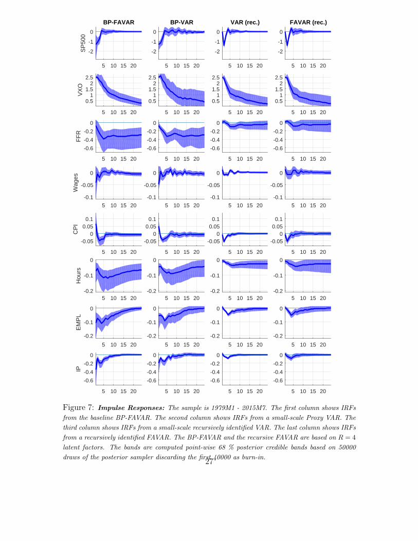
Figure 7: Impulse Responses: The sample is 1979M1 - 2015M7. The first column shows IRFs

from the baseline BP-FAVAR. The second column shows IRFs from a small-scale Proxy VAR. The

third column shows IRFs from a small-scale recursively identified VAR. The last column shows IRFs

from a recursively identified FAVAR. The BP-FAVAR and the recursive FAVAR are based on R = 4

latent factors. The bands are computed point-wise 68 % posterior credible bands based on 50000

draws of the posterior sampler discarding the first 40000 as burn-in.27

The uncertainty shock is ordered second, i.e. after the S&P500 index. This assumes

that the stock market does not react within a month to an exogenous increase in

uncertainty and that financial shocks are the only shocks, apart from the uncertainty

shock itself, which influence the uncertainty measure within the month. Differences

between the BP-FAVAR and the recursive VAR can be driven by both informational

and identification issues.

Recursively identified FAVAR. This scheme adds R latent factor to the small-

scale VAR while keeping B lower-triangular. The uncertainty shock is ordered in

position R+2, i.e. after the latent factors and the S&P500 index. This assumes that

neither the latent factors nor the stock market react within a month to an exoge-

nous increase in uncertainty. Differences between the BP-FAVAR and the recursive

FAVAR in the impact effects of shocks will be driven primarily by the identification

scheme.

Figure 7 shows the impulse responses obtained from the baseline and the three

benchmark models: The response variables are those employed by Bloom (2009),

Piffer and Podstawski (forthcoming) and other studies. The shock is normalized to

generate an increase of 2.5 in the VXO on impact, which is comparable in magnitude

to these studies. Estimation is based on 50000 Gibbs draws, discarding the first 40000

draws as a burn-in sample, as in Belviso and Milani (2006) and Ahmadi and Uhlig

(2015).

All four models replicate the main findings of Bloom (2009): A rapid drop and

subsequent rebound of employment, production and hours worked. It is also in line

with Basu and Bundick (2017) who argue that the co-movement among these vari-

ables is a key empirical feature that theoretical models should be able to reproduce.

For the stock market, the two recursively identified models (column 3 and 4)

exclude an on-impact effect of the uncertainty shock on the stock market index.

This results in a biased reaction of the S&P 500 index: The models identified via a

proxy (columns 1 and 2) show that the stock market reacts on impact and quickly

rebounds. This is in line with the fast moving nature of financial markets, which

price increases in uncertainty within the period.

For the real variables, the recursive scheme suggests a moderate negative reaction

28

of hours, employment and industrial production of less than -0.05%. In the two

models identified via proxies this reaction is estimated to be up to -0.2% for industrial

production and roughly -0.1% for hours and employment. Given the similarity in

the price reaction across models, the recursive models provide a skewed view of the

nominal and real interactions following an uncertainty shock.

The inclusion of factors does not qualitatively alter the results. The BP-FAVAR

produces results broadly in line with the BP-VAR. The biases resulting from a re-

cursive identification in the small-scale VAR cannot be alleviated by the inclusion of

factors. As pointed out by Sims (2012), informational insufficiency is not an either/or

concept but can have quantitatively very different effects on impulse responses, de-

pending on the application. In the present case, statistical tests detect informational

insufficiency, but alleviating this issue does not have a severe quantitative impact.

All in all, the results are comforting news for policy makers who employ instru-

ments that affect real and nominal variables in the same direction. For example,

a Central Bank could use an expansionary policy when faced with an increase in

uncertainty and thus move both inflation and real variables closer to their respective

targets.

4 Conclusion

This paper aims at recovering the interrelations between real and nominal variables

following an identified uncertainty shock by employing a Bayesian Proxy FAVAR.

The first contribution is the empirical finding that uncertainty shocks are de-

flationary in the short run and indistinguishable from zero after six months. This

finding relates to the work by Born and Pfeifer (2014) and Fernandez-Villaverde et al.

(2015) who show in a theoretical modelling framework that the inflationary effects of

uncertainty shocks are driven by two opposing channels: an aggregate demand and

a price-bias channel. The aggregate effect of these two channels is unknown ex ante.

My results lend empirical support to the dominance of the aggregate demand over

the price-bias channel.

My second contribution is methodological. I combine a recent strand of the

29

Bayesian VAR literature that uses external instruments for identification (Caldara

and Herbst, forthcoming) with the Bayesian factor model literature (Belviso and

Milani, 2006, Ahmadi and Uhlig, 2015). I show how a state-space model can be

set up to jointly exploit the advantages of both approaches. The resulting Bayesian

Proxy factor-augmented VAR model avoids two shortcomings of commonly employed

small-scale recursively identified VAR models, namely a non-credible identification

scheme and informational insufficiency. I detect informational insufficiency of the

small-scale workhorse model, but find that it has limited quantitative impacts on

the impulse responses. This relates to the work by Sims (2012) who also finds that

informational deficiency is not an either/or but a quantitative issue.

Future empirical research concerned with the identification of uncertainty shocks

in a structural VAR context, especially if it is conducted with few variables, should

pay close attention to the information set. Informational insufficiency is detected

even in the relatively rich workhorse model by Bloom (2009). While it has only

limited quantitative impacts in this case, this might be very different when reducing

the information set.

From a methodological point of view, the BP-FAVAR model offers potential for a

number of extensions: First, identification of two or more shocks is generally possible

in this setup. As pointed out by Kilian and Lutkepohl (2017), avoiding non-credible

short-run exclusion restrictions is particularly important in factor models. Therefore,

the BP-FAVAR could be extended to identify multiple shocks via external instru-

ments. Second, a combination of proxies with sign restrictions in this context is a

natural point of departure given the similarity in model setup between the BP-VAR

and VARs identified via sign restrictions. The combination of these two approaches

is likely to lead to sharper inference.

30

References

Ahmadi, P. A. and Uhlig, H. (2015), Sign restrictions in bayesian favars with an

application to monetary policy shocks, Technical report, National Bureau of Eco-

nomic Research.

Angelini, G., Bacchiocchi, E., Caggiano, G. and Fanelli, L. (2018), ‘Uncertainty

across volatility regimes’.

Bachmann, R. and Bayer, C. (2013), ‘wait-and-see business cycles?’, Journal of Mon-

etary Economics 60(6), 704–719.

Bachmann, R. and Sims, E. R. (2012), ‘Confidence and the transmission of govern-

ment spending shocks’, Journal of Monetary Economics 59(3), 235–249.

Baker, S. R., Bloom, N. and Davis, S. J. (2016), ‘Measuring economic policy uncer-

tainty’, The Quarterly Journal of Economics 131(4), 1593–1636.

Basu, S. and Bundick, B. (2017), ‘Uncertainty shocks in a model of effective demand’,

Econometrica 85(3), 937–958.

Baumeister, C. and Hamilton, J. D. (2015), ‘Sign restrictions, structural vector au-

toregressions, and useful prior information’, Econometrica 83(5), 1963–1999.

Belviso, F. and Milani, F. (2006), ‘Structural factor-augmented vars (sfavars) and

the effects of monetary policy’, Topics in Macroeconomics 6(3).

Bernanke, B. S., Boivin, J. and Eliasz, P. (2005), ‘Measuring the effects of monetary

policy: a factor-augmented vector autoregressive (favar) approach’, The Quarterly

Journal of Economics 120(1), 387–422.

Bloom, N. (2009), ‘The impact of uncertainty shocks’, Econometrica 77(3), 623–685.

Boivin, J., Giannoni, M. P. and Mihov, I. (2009), ‘Sticky prices and monetary policy:

Evidence from disaggregated us data’, The American Economic Review 99(1), 350–

384.

31

Born, B. and Pfeifer, J. (2014), ‘Policy risk and the business cycle’, Journal of

Monetary Economics 68, 68–85.

Braun, R., Bruggemann, R. et al. (2017), Identification of svar models by combin-

ing sign restrictions with external instruments, Technical report, Department of

Economics, University of Konstanz.

Caggiano, G., Castelnuovo, E. and Nodari, G. (2017), ‘Uncertainty and monetary

policy in good and bad times’.

Caggiano, G., Castelnuovo, E. and Pellegrino, G. (2017), ‘Estimating the real ef-

fects of uncertainty shocks at the zero lower bound’, European Economic Review

100, 257–272.

Caldara, D. and Herbst, E. (forthcoming), ‘Monetary policy, real activity, and

credit spreads: Evidence from bayesian proxy svars’, American Economic Journal:

Macroeconomics .

Carter, C. K. and Kohn, R. (1994), ‘On gibbs sampling for state space models’,

Biometrika 81(3), 541–553.

Christiano, L. J., Motto, R. and Rostagno, M. (2014), ‘Risk shocks’, American Eco-

nomic Review 104(1), 27–65.

Cowles, M. K. and Carlin, B. P. (1996), ‘Markov chain monte carlo convergence

diagnostics: a comparative review’, Journal of the American Statistical Association

91(434), 883–904.

Fernandez-Villaverde, J., Guerron-Quintana, P., Kuester, K. and Rubio-Ramırez, J.

(2015), ‘Fiscal volatility shocks and economic activity’, The American Economic

Review 105(11), 3352–3384.

Forni, M. and Gambetti, L. (2014), ‘Sufficient information in structural vars’, Journal

of Monetary Economics 66, 124–136.

32

Fruhwirth-Schnatter, S. (1994), ‘Data augmentation and dynamic linear models’,

Journal of time series analysis 15(2), 183–202.

Gelper, S. and Croux, C. (2007), ‘Multivariate out-of-sample tests for granger causal-

ity’, Computational statistics & data analysis 51(7), 3319–3329.

Geman, S. and Geman, D. (1984), ‘Stochastic relaxation, gibbs distributions, and

the bayesian restoration of images’, IEEE Transactions on pattern analysis and

machine intelligence (6), 721–741.

Geweke, J. (1992), Evaluating the accuracy of sampling-based approaches to the

calculation of posterior moments, in ‘BAYESIAN STATISTICS’, Citeseer.

Huber, F. and Fischer, M. M. (2018), ‘A markov switching factor-augmented var

model for analyzing us business cycles and monetary policy’, Oxford Bulletin of

Economics and Statistics 80(3), 575–604.

Jurado, K., Ludvigson, S. C. and Ng, S. (2015), ‘Measuring uncertainty’, The Amer-

ican Economic Review 105(3), 1177–1216.

Kilian, L. and Lutkepohl, H. (2017), Structural vector autoregressive analysis, Cam-

bridge University Press.

Koop, G. (2003), Bayesian Econometrics, John Wiley & Sons Ltd,.

Koop, G., Korobilis, D. et al. (2010), ‘Bayesian multivariate time series methods for

empirical macroeconomics’, Foundations and Trends in Econometrics 3(4), 267–

358.

Leduc, S. and Liu, Z. (2016), ‘Uncertainty shocks are aggregate demand shocks’,

Journal of Monetary Economics 82, 20–35.

Ludvigson, S. C., Ma, S. and Ng, S. (2018), Uncertainty and business cycles: ex-

ogenous impulse or endogenous response?, Technical report, National Bureau of

Economic Research.

33

McCracken, M. W. and Ng, S. (2016), ‘Fred-md: A monthly database for macroeco-

nomic research’, Journal of Business & Economic Statistics 34(4), 574–589.

Piffer, M. and Podstawski, M. (forthcoming), ‘Identifying uncertainty shocks using

the price of gold’, Economic Journal .

Rubio-Ramirez, J. F., Waggoner, D. F. and Zha, T. (2010), ‘Structural vector au-

toregressions: Theory of identification and algorithms for inference’, The Review

of Economic Studies 77(2), 665–696.

Sims, E. R. (2012), News, non-invertibility, and structural vars, in ‘DSGE Models

in Macroeconomics: Estimation, Evaluation, and New Developments’, Emerald

Group Publishing Limited, pp. 81–135.

Stock, J. H. and Watson, M. W. (2012), Disentangling the channels of the 2007-2009

recession, Technical report, National Bureau of Economic Research.

Stock, J. H. and Watson, M. W. (2016), ‘Dynamic factor models, factor-augmented

vector autoregressions, and structural vector autoregressions in macroeconomics’,

Handbook of macroeconomics 2, 415–525.

Wu, J. C. and Xia, F. D. (2016), ‘Measuring the macroeconomic impact of monetary

policy at the zero lower bound’, Journal of Money, Credit and Banking 48(2-

3), 253–291.

Yamamoto, Y. (forthcoming), ‘Bootstrap inference for impulse response functions in

factor-augmented vector autoregressions’, Journal of Applied Econometrics .

34

1960 1970 1980 1990 2000 2010-0.05

0

0.05

Gold Price Proxy

1960 1970 1980 1990 2000 2010-10

0102030

Innovations to VXO

1960 1970 1980 1990 2000 2010

-500

50100150

Innovations to Policy Uncertainty

Figure 8: Uncertainty Proxies The top panel shows the baseline gold price proxy for uncertainty

by Piffer and Podstawski (forthcoming). The middle panel shows the Stock and Watson (2012)

uncertainty proxy computed as residuals of an AR(2) process of the VXO. The bottom panel shows

the Stock and Watson (2012) uncertainty proxy computed as residuals of an AR(2) process of the

Baker et al. (2016) policy uncertainty proxy. All proxies are winsorized at the 10 % level.

A Robustness Checks

A.1 Stock and Watson (2012) Instruments

Stock and Watson (2012) were the first to propose two proxies for uncertainty shocks.

They employ the innovations in the VXO and in the policy uncertainty index by

Baker et al. (2016). These innovations are computed as residuals from an AR(2)

process. While innovations to the VXO are likely to be correlated with the uncer-

tainty shocks of interest in this study, this is less likely for the policy uncertainty

instrument. The reason is that the concept of uncertainty it is designed to approx-

imate differs from the one I have in mind in this study. Thus, in analysing impulse

responses, I concentrate on innovations to the VXO.

I reproduce the instrument as follows: In a first step I estimate an AR(2) process

35

5 10 15 20-2

-1

0

S&

P 5

00

5 10 15 200

1

2

VX

O

5 10 15 20

-0.2

-0.1

0F

ed fu

nds

rate

5 10 15 20

-0.020

0.02

Wag

e

5 10 15 20

-0.06-0.04-0.02

00.02

CP

I

5 10 15 20-0.08-0.06-0.04-0.02

00.02

Hou

rs

5 10 15 20

-0.06-0.04-0.02

00.020.04

Em

ploy

men

t

5 10 15 20

-0.1

0

0.1

Ind.

Pro

duct

ion

Figure 9: Stock and Watson (2012) innovations to the VXO The model is specified as in

the baseline with the gold price proxy replaced by the Stock and Watson (2012) VXO innovations.

These are computed as the residuals from an AR(2) process of the VXO.

including a constant for the VXO index as in Stock and Watson (2012). In a second

step, I truncate the proxy at the 10th and 90th percentile and set all observations

within these two quantiles to zero. This is to ensure that the proxy only captures

quantitatively relevant spikes in uncertainty.

Figure 8 plots the resulting proxies while Table 2 shows the correlations among the

proxies. The instruments have some degree of correlation, but they clearly measure

distinct variations in uncertainty.

Table 2: Correlation among proxies

Gold proxy 1.00VXO innovations 0.38 1.00

Policy Uncertainty innovations 0.50 0.37 1.00

Figure 9 shows the impulse response functions when employing the innovations

36

to the VXO as proxies. While the identification of the impact effects is not as sharp

as in the baseline, the dynamics are broadly similar.

A.2 Increasing the Lag Length

In order to assess robustness with respect to the lag length, I set P = 9. Figure 10

shows that the main results remain unchanged.

A.3 Alternative Uncertainty Measures

Jurado et al. (2015) argue that indices like the VXO used in the baseline do not

accurately capture the type of macroeconomic uncertainty that the researcher is

interested in. They propose alternative indeces based on large panels of time series.

Jurado et al. (2015) provide indeces extracted from macro series and Ludvigson et al.

(2018) provide indeces extracted from financial and real series.9 Figure 11 shows that

they are highly correlated over the whole sample period.

Figure 12 replaces the VXO by the macro uncertainty index, Figure 13 replaces

the VXO by the financial uncertainty index and Figure 14 replaces it by the real

uncertainty index. The results remain qualitatively unchanged.

B Conditional likelihood of mt

This section re-parametrises Caldara and Herbst (forthcoming) to allow for iden-

tification of impact effects. For the posterior sampler, we will need to be able to

evaluate the conditional likelihood of mt given yt.

9Details can be found here https://www.sydneyludvigson.com/data-and-appendixes/

37

5 10 15 20-3-2-101

SP

500

BP-FAVAR

5 10 15 20-3-2-101

BP-VAR

5 10 15 20-3-2-101

VAR (rec.)

5 10 15 20-3-2-101

FAVAR (rec.)

5 10 15 20

0

1

2

3

VX

O

5 10 15 20

0

1

2

3

5 10 15 20

0

1

2

3

5 10 15 20

0

1

2

3

5 10 15 20

-0.8-0.6-0.4-0.2

0

FF

R

5 10 15 20

-0.8-0.6-0.4-0.2

0

5 10 15 20

-0.8-0.6-0.4-0.2

0

5 10 15 20

-0.8-0.6-0.4-0.2

0

5 10 15 20

-0.2

-0.1

0

Wag

es

5 10 15 20

-0.2

-0.1

0

5 10 15 20

-0.2

-0.1

0

5 10 15 20

-0.2

-0.1

0

5 10 15 20

-0.1

0

0.1

CP

I

5 10 15 20

-0.1

0

0.1

5 10 15 20

-0.1

0

0.1

5 10 15 20

-0.1

0

0.1

5 10 15 20

-0.2

-0.1

0

Hou

rs

5 10 15 20

-0.2

-0.1

0

5 10 15 20

-0.2

-0.1

0

5 10 15 20

-0.2

-0.1

0

5 10 15 20

-0.15-0.1

-0.050

EM

PL

5 10 15 20

-0.15-0.1

-0.050

5 10 15 20

-0.15-0.1

-0.050

5 10 15 20

-0.15-0.1

-0.050

5 10 15 20-0.6

-0.4

-0.2

0

IP

5 10 15 20-0.6

-0.4

-0.2

0

5 10 15 20-0.6

-0.4

-0.2

0

5 10 15 20-0.6

-0.4

-0.2

0

Figure 10: Impulse Responses (P=9): The sample is 1979M1 - 2015M7. The first column

shows IRFs from the baseline BP-FAVAR. The second column shows IRFs from a small-scale Proxy

VAR. The third column shows IRFs from a small-scale recursively identified VAR. The last column

shows IRFs from a recursively identifed FAVAR. The bands are computed point-wise 68 % posterior

credible bands based on 10000 draws of the posterior sampler.

38

1965 1970 1975 1980 1985 1990 1995 2000 2005 2010 2015

10

20

30

40

50

60

Uncertainty Measures

FinUncMacUncRealUncVXO

Figure 11: Uncertainty Measures The uncertainty measures are taken from Ludvigson et al.

(2018) and rescaled to match the mean of the VXO for comparability.

Restate the model for convenience:

xt = Λyt + ξt (58)[yt

mt

]=

[Π 0

0 0

][wt

mt−1

]+

[B β

β′ σν

][εt

νt

](59)

V ar(

[yt −Πwt

mt

]) =

[Σ Bβ′

βB′ β′β + σ2ν

], (60)

where β = [β 0]′

The likelihood is invariant to observationally equivalent rotations ofB. Therefore

we can replace B = BcQ, where Bc is, for example, the lower-triangular Cholesky

decomposition of Σ.

V ar(

[yt −Πwt

mt

]) =

[Σ BcQβ′

βQ′Bc′ β′β + σ2ν

](61)

39

5 10 15 20

-10-50

S&

P 5

005 10 15 20

02468

Mac

Unc

5 10 15 20-3-2-10

Fed

fund

s ra

te

5 10 15 20

-0.6-0.4-0.2

0

Wag

e

5 10 15 20

0

0.5

1

CP

I

5 10 15 20-0.8-0.6-0.4-0.2

00.2

Hou

rs

5 10 15 20

-1

-0.5

0

Em

ploy

men

t

5 10 15 20

-2

-1

0

Ind.

Pro

duct

ion

Figure 12: Macroeconomic Uncertainty The model is specified as in the baseline with VXO

replaced by the macroeconomic uncertainty indicator by Ludvigson et al. (2018).

Then, using the rules for the conditional mean of multivariate normal distributions,

we obtain the conditional likelihood

mt|yt,Π,Σ, b, β, σν ∼ N(µm|Y , Vm|Y ), (62)

µm|Y = βQ′Bc′Σ−1ut (63)

= βε1,t (64)

Vm|Y = bb′ + σ2ν − bQ′Bc′Σ−1BcQb′ (65)

= σ2ν (66)

Note that, once we condition on yt, the likelihood of mt does not depend on xt.

In addition, note that the conditional likelihood of mt does not depend on the full

matrix B, but only on its first column, b because the model is partially identified.

40

5 10 15 20

-8-6-4-202

S&

P 5

005 10 15 20

0246

Fin

Unc

5 10 15 20

-2

-1

0F

ed fu

nds

rate

5 10 15 20

-0.4-0.2

0

Wag

e

5 10 15 20-0.2

00.20.40.60.8

CP

I

5 10 15 20

-0.6-0.4-0.2

0

Hou

rs

5 10 15 20

-0.6-0.4-0.2

0

Em

ploy

men

t

5 10 15 20

-2

-1

0

Ind.

Pro

duct

ion

Figure 13: Financial Uncertainty The model is specified as in the baseline with VXO replaced

by the financial uncertainty indicator by Ludvigson et al. (2018).

Therefore, we can rewrite (62) as

mt|yt,Π,Σ, b, β, σν ∼ N(µm|Y , Vm|Y ), (67)

C Metropolis-within-Gibbs sampler for the BP-

FAVAR

This section outlines the posterior sampling procedure for the Bayesian Proxy Factor

Augmented VAR. It combines posterior samplers for Bayesian FAVARs, e.g. Koop

et al. (2010) and Ahmadi and Uhlig (2015) with the algorithm for Bayesian Proxy

VARs proposed by Caldara and Herbst (forthcoming). It provides posterior draws

of the parameters [Π,Σ,Ω,Λ, β, σν ] as well as of the factors yt.

41

5 10 15 20

-8-6-4-20

S&

P 5

005 10 15 20

024

Rea

lUnc

5 10 15 20

-2

-1

0F

ed fu

nds

rate

5 10 15 20

-0.4-0.2

0

Wag

e

5 10 15 20-0.2

00.20.4

CP

I

5 10 15 20-0.6-0.4-0.2

0

Hou

rs

5 10 15 20

-0.6-0.4-0.2

0

Em

ploy

men

t

5 10 15 20

-2

-1

0

Ind.

Pro

duct

ion

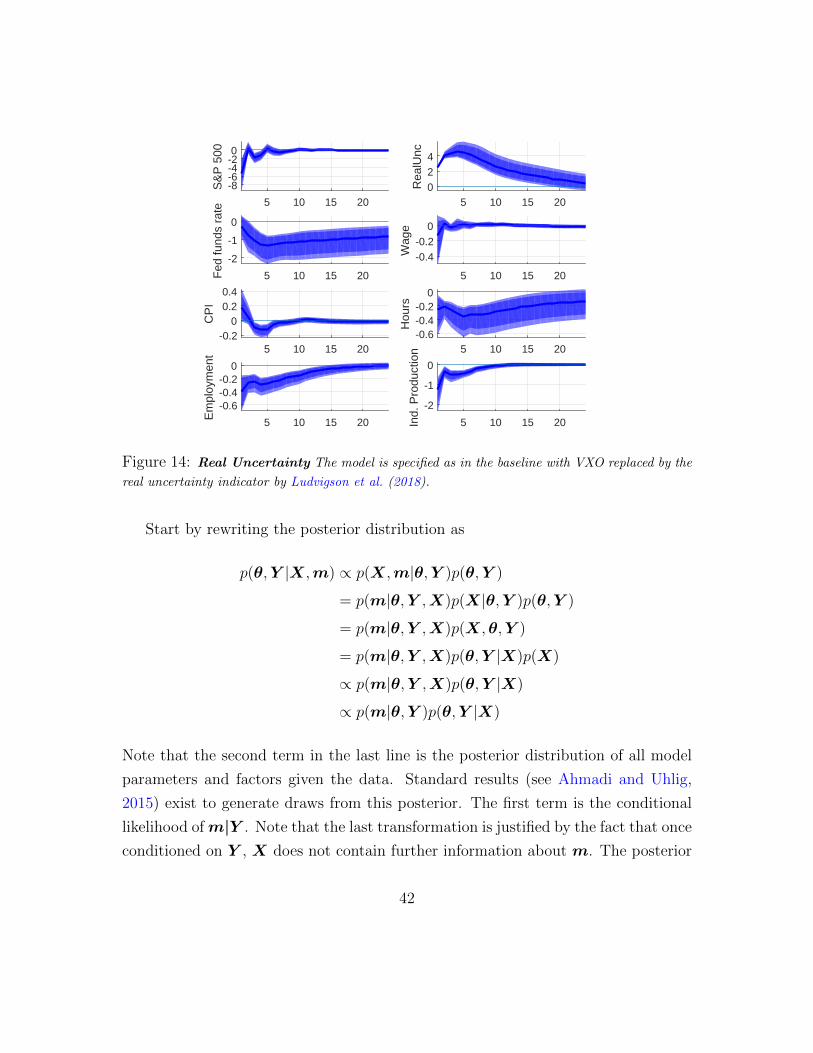
Figure 14: Real Uncertainty The model is specified as in the baseline with VXO replaced by the

real uncertainty indicator by Ludvigson et al. (2018).

Start by rewriting the posterior distribution as

p(θ,Y |X,m) ∝ p(X,m|θ,Y )p(θ,Y )

= p(m|θ,Y ,X)p(X|θ,Y )p(θ,Y )

= p(m|θ,Y ,X)p(X,θ,Y )

= p(m|θ,Y ,X)p(θ,Y |X)p(X)

∝ p(m|θ,Y ,X)p(θ,Y |X)

∝ p(m|θ,Y )p(θ,Y |X)

Note that the second term in the last line is the posterior distribution of all model

parameters and factors given the data. Standard results (see Ahmadi and Uhlig,

2015) exist to generate draws from this posterior. The first term is the conditional

likelihood ofm|Y . Note that the last transformation is justified by the fact that once

conditioned on Y , X does not contain further information about m. The posterior

42

sampler weights draws from p(θ,Y |X) with the conditional likelihood of m|Y using

an independence Metropolis-Hastings step as in Caldara and Herbst (forthcoming).

It is in this sense that m informs the estimation of reduced form parameters.

1. Set starting values

In order to obtain starting values of the reduced form parameters [Π,Σ,Ω,Λ],

I estimate the model once using the two-step-procedure proposed by Boivin

et al. (2009), which takes the restrictions implied by the observation equation

into account when extracting factors. I use Principal Component Analysis to

obtain R factors fPCt from xt and the factor loadings ΛPC . Then run the

regression

xt = const+ ΛffPCt + Λzzt + vt

and construct X = ΛffPCt , the fitted values orthogonalized with respect to the

observable factors. Then extract R factors from X and repeat the procedure

20 times as in Boivin et al. (2009). Save [Λ0,f 0t ,Ω

0]

Lastly, estimate a reduced-form VAR in y0t =

[f 0t

zt

]to obtain [Σ0,Π0].

For the remaining parameters, I start the algorithm from β0 = 0, σ0ν =

0.5std(mt) (Caldara and Herbst, forthcoming call this the ”high relevance

prior”, which imposes that half the variance in the proxy can be attributed

to measurement error)

At each stage j proceed with the following steps:

2. Draw f jt using the Carter-Kohn backward recursion of the Kalman filter. Set

yjt =

[f jt

zt

]3. Draw Λj from its conditional normal posterior given in equation 27.

λi|ωj−1ii ,X,Y ∼ N(µλ,i,Ωiij−1M−1i )

43

Impose the normalisation on Λ.

4. Compute ξjt = xt − Λjyjt and draw the diagonal elements of Ω from their

posterior inverse Gamma distributions

ωii|X,Y ∼ IG(sci/2, shi/2)

5. Sample Σcand from an inverse Wishart

Σcand ∼ IW (S, τ)

6. Sample Πcand from a multivariate normal using the Minnesota values as priors

for the posterior covariance.

vec(Πcand) ∼ N(µΠ, V Π)

7. With probability α set Πj = Πcand and Σj = Σcand, otherwise set Πj = Πj−1

and Σj = Σj−1, where

α = min(p(m,Y |Πcand,Σcand,Qj−1)

p(m,Y |Πj−1,Σj−1,Qj−1), 1)

8. Draw Qcand·,1 as the first column of an orthogonal matrix form a uniform Haar

distribution using the algorithm by Rubio-Ramirez et al. (2010). Set Qj·,1 =

Qcand·,1 with probability α and Qj

·,1 = Qj−1·,1 else.

α = min(p(m,Y |Πj,Σj,Qcand

·,1 )

p(m,Y |Πj,Σj,Qj−1·,1 )

, 1)

9. Compute structural errors εjt = (chol(Σj)Qj·,1)−1U j. Draw βj from its posterior

44

normal distribution

βj ∼ N(µβ, σβ)

10. Draw σjν from its posterior inverse Gamma distribution

σjν ∼ IG(sh, sc)

D Multivariate out-of-sample Granger-causality test

We would like to assess whether a vector f t Granger-causes a vector zt. The series

f t is said to Granger-cause the series zt if the past of f t has additional power for

forecasting zt after controlling for the past of zt. Gelper and Croux (2007) base their

test statistic on the comparison of two nested VAR models:

zt = Φ(L)zt−1 + vrt (68)

zt = Φ(L)zt−1 + Ψ(L)f t−1 + vft (69)

The restricted model (68) has only past values of zt as regressors, while the unre-

stricted model (69) has both the past of zt and f t as regressors. vrt are the residuals

of the restricted, while vft are the residuals of the full model. The test statistic is

based on the out-of-sample forecast performance of these two models. Compared to

in-sample tests, this approach is less susceptible to overfitting.

The unrestricted model can be written out as

zt = φ0 + φ1zt−1 + ...+ φpzt−p +ψ1f t−1 + ...+ψpf t−p + vft (70)

where φj, j = 0, ..., p are of dimension K×K and ψj are of dimension K×R. Then

the Null hypothesis of no Granger causality can be written as

H0 : ψ1 = ψ2 = · · · = ψp = 0 (71)

45

The out-of-sample test proceeds as follows: First, split the sample in half as T =

T1 + T2, where T1 = T2 = 0.5T (assuming T is even) and construct one-step-ahead

forecasts zrT1+1 and zfT1+1 based on the restricted and the full model, respectively.

Then, expand the estimation sample by one and construct zrT1+2 and zfT1+2. The

last forecasts, zrT and zfT are based on an estimation sample of size T − 1. As a

second step, construct the series of one-step-ahead forecast errors vrt = zrt − zt and

vf = zft − zt for the two competing models and save them in the vectors vr and

vf of size T2. As a third step, construct the test statistic comparing the forecasting

performance of the two models as

MSFE = log(|vr′vr||vf ′vf |

), (72)

where MSFE is the mean squared forecast error and | · | stands for the determinant

of a matrix. If the full model provides better forecasts, MSFE takes a larger value,

indicating Granger-causality.

The asymptotic distribution of the test statistic is unknown. Critical values will

therefore be based on a residual bootstrap. It proceeds in the following steps:

1. Estimate the model under the Null, i.e. model (68) and compute the test

statistic, denoted here by s0, as described above

2. Generate Nb = 1000 new time series z∗1, ...,z∗t according to model (68) using

the parameter estimates and resampling the residuals with replacement. For

each bootstrap sample, compute the test statistic resulting in s∗1, ..., s∗Nb

3. The percentage of bootstrap test statistics, s∗1, ..., s∗Nb, exceeding s0 is an ap-

proximation of the p-value.

Gelper and Croux (2007) show that the test performs well in a Monte Carlo

setting as well as in an application to real data.

46

E Carter-Kohn Algorithm

This section lays out the Carter-Kohn algorithm. It is used to sample the factors

Y given all model parameters, θ, and the data, X, i.e. it generates draws from

p(Y |θ,X).

E.1 State-space form

Start by rewriting observation and transition equation as[xt

zt

]= HBt +Wt (73)

Bt = FBt−1 + Vt (74)

V ar(Wt) = R (75)

V ar(Vt) = Q (76)

where

H =

[Λf Λz 0 ... 0

0 I 0 ... 0

]; Bt =

[β′t β′t−1 ... β′t−p

]′; βt =

[f t

zt

]

Wt =

[ξt

0

]; F =

[Π

I 0 0

]; Vt =

[ut

0

]

R =

[Ω 0

0 0

]; Q =

[Σ 0

0 0

]Then consider the following factorisation:

p(B1:T |X,θ) = p(BT |x1:T ,θ)T−1∏t=1

p(Bt|Bt+1, X, θ) (77)

47

Given the linear Gaussian form of the state space model we have that

BT |x1:T , θ ∼ N(BT |T ,PT |T ) (78)

Bt|T |Bt+1|T ,x1:T , θ ∼ N(Bt|t,Bt+1|T ,Pt|t,Bt+1|T ) (79)

with

BT |T = E(BT |x1:T ,θ) (80)

PT |T = Cov(BT |x1:T ,θ) (81)

Bt|t,Bt+1|T = E(Bt|Bt|t,Bt+1|t,θ) (82)

Pt|t,Bt+1|T = Cov(Bt|Bt|t,Bt+1|t,θ) (83)

E.2 Kalman-filter

In a first step, we can run a Kalman filter to obtain a series of Kalman-filtered draws

of the state variable Bt Bt|t for t = 1, ...T . To initialise, we set B1|0 = 0 and P1|0 = I.

Then, iterate forward as:

Bt|t = Bt|t−1 + κt|t−1ηt|t−1 (84)

where ηt|t−1 = Bt − FBt|t−1 denotes the forecast error, ft|t−1 = HPt|t−1H′ + R its

variance and κt|t−1 = Pt|t−1Hf−1t|t−1 the ”Kalman-gain”

Pt|t−1 = FPt−1|t−1F ′ +Q (85)

Then, conditioning on the last of these Kalman-filtered draws, BT |T and PT |T , we

can run the filter backwards to obtain a series Bt|t+1 for t = 1, ..., T − 1 as follows:

B∗t|t,Bt+1|T = Bt|t + Pt|tF∗′J−1t+1|tψt+1|t (86)

P∗t|t,Bt+1|T = Pt|t − Pt|tF∗′J−1t+1|tF

∗Pt|t (87)

48

where ψt+1|t = B∗t+1 − F∗Bt|t and Jt+1|t = F∗Pt|tF∗′+ Q∗. Note that Q∗ refers to

the top R × R block of Q and that F∗ and B∗ denote the first R rows of F and B,

respectively. This is required because Q is singular given the presence of observable

factors.

Plugging these draws into (77) results in an unconditional posterior draw of the

state variable, B1, ...,BT . Its top R+K block represents an unconditional posterior

draw of factors, yt.

E.3 Convergence of the Posterior Sampling Algorithm

The convergence properties of the reduced form parameters of a Bayesian FAVAR

model are discussed in detail in Ahmadi and Uhlig (2015). They show that a Gibbs

sampling procedure, similar to the one employed for the reduced form parameters

here, converges for appropriate lengths of the sampler. The convergence properties

of the structural parameters, however, need to be assessed. In particular the first col-

umn of B containing the on-impact effects of the shock of interest are of importance.

In order to do so, I follow Ahmadi and Uhlig (2015) and employ the convergence

diagnostic proposed by Geweke (1992). A detailed discussion of this convergence

diagnostic can be found, for example, in Cowles and Carlin (1996).

This diagnostic assesses the convergence of each element ηi of parameter vector,

η. The assessment is based on a comparison of means across different parts of this

chain. If the means are close to each other, the procedure detects convergence.

In a first step, extract from each (univariate) posterior draw ηiDi=1 the fol-

lowing subseries: η1i, ..., η0.1D,i, i.e. the first 10 % of draws for parameter i, and

η0.6D+1,i, ..., ηD,i, i.e. the last 40% of draws, where D is the length of the MCMC

chain. Compute µfirst and µlast, the mean, as well as σfirst and σlast, the standard

deviation, of these subseries. Then the test statistic is

CD =µfirst − µlastσfirst√0.1D

+ σlast√0.4D

(88)

Under the conditions mentioned in Geweke (1992), CD has an asymptotic standard

49

normal distribution

The final output is a p-value indicating whether or not we can reject the Null hy-

pothesis of convergence, i.e. equality of mean across the chain, at a given significance

level.

Table 3 shows that for 10 out of 12 parameters, the Null of convergence cannot

be rejected. Note that the first R parameters refer to the on-impact effect on the

latent factors, which do not have an economic interpretation.

p-value

r=1 0.7348r=2 0.0007r=3 0.1343r=4 0.1363k=1 0.8634k=2 0.1635k=3 0.7797k=4 0.0871k=5 0.3087k=6 0.9196k=7 0.0444k=8 0.1515

Table 3: Geweke (1992) test for convergence of the MCMC chain The sample split is

T = T1 + T2 + T3, where T1 = 0.1T , T2 = 0.5T and T3 = 0.4T . P-values are computed as quantiles

of a Chi-squared distribution.

50

F Data Description

Table 4: Data

Output and Income

id tcode fred description

1 5 RPI Real Personal Income2 5 W875RX1 Real personal income ex transfer receipts6 5 INDPRO IP Index7 5 IPFPNSS IP: Final Products and Nonindustrial Supplies8 5 IPFINAL IP: Final Products (Market Group)9 5 IPCONGD IP: Consumer Goods10 5 IPDCONGD IP: Durable Consumer Goods11 5 IPNCONGD IP: Nondurable Consumer Goods12 5 IPBUSEQ IP: Business Equipment13 5 IPMAT IP: Materials14 5 IPDMAT IP: Durable Materials15 5 IPNMAT IP: Nondurable Materials16 5 IPMANSICS IP: Manufacturing (SIC)17 5 IPB51222s IP: Residential Utilities18 5 IPFUELS IP: Fuels19 1 NAPMPI ISM Manufacturing: Production Index20 2 CUMFNS Capacity Utilization: Manufacturing

51

Labor Market

id tcode fred description

21* 2 HWI Help-Wanted Index for United States22* 2 HWIURATIO Ratio of Help Wanted/No. Unemployed23 5 CLF16OV Civilian Labor Force24 5 CE16OV Civilian Employment25 2 UNRATE Civilian Unemployment Rate26 2 UEMPMEAN Average Duration of Unemployment (Weeks)27 5 UEMPLT5 Civilians Unemployed - Less Than 5 Weeks28 5 UEMP5TO14 Civilians Unemployed for 5-14 Weeks29 5 UEMP15OV Civilians Unemployed - 15 Weeks & Over30 5 UEMP15T26 Civilians Unemployed for 15-26 Weeks31 5 UEMP27OV Civilians Unemployed for 27 Weeks and Over32* 5 CLAIMSx Initial Claims33 5 PAYEMS All Employees: Total nonfarm34 5 USGOOD All Employees: Goods-Producing Industries35 5 CES1021000001 All Employees: Mining and Logging: Mining36 5 USCONS All Employees: Construction37 5 MANEMP All Employees: Manufacturing38 5 DMANEMP All Employees: Durable goods39 5 NDMANEMP All Employees: Nondurable goods40 5 SRVPRD All Employees: Service-Providing Industries41 5 USTPU All Employees: Trade, Transportation & Utilities42 5 USWTRADE All Employees: Wholesale Trade43 5 USTRADE All Employees: Retail Trade44 5 USFIRE All Employees: Financial Activities45 5 USGOVT All Employees: Government46 1 CES0600000007 Avg Weekly Hours : Goods-Producing47 2 AWOTMAN Avg Weekly Overtime Hours : Manufacturing48 1 AWHMAN Avg Weekly Hours : Manufacturing49 1 NAPMEI ISM Manufacturing: Employment Index127 6 CES0600000008 Avg Hourly Earnings : Goods-Producing128 6 CES2000000008 Avg Hourly Earnings : Construction129 6 CES3000000008 Avg Hourly Earnings : Manufacturing

52

Housing

id tcode fred description

50 4 HOUST Housing Starts: Total New Privately Owned51 4 HOUSTNE Housing Starts, Northeast52 4 HOUSTMW Housing Starts, Midwest53 4 HOUSTS Housing Starts, South54 4 HOUSTW Housing Starts, West55 4 PERMIT New Private Housing Permits (SAAR)56 4 PERMITNE New Private Housing Permits, Northeast (SAAR)57 4 PERMITMW New Private Housing Permits, Midwest (SAAR)58 4 PERMITS New Private Housing Permits, South (SAAR)59 4 PERMITW New Private Housing Permits, West (SAAR)

Consumption, Orders and inventories

3 5 DPCERA3M086SBEA Real personal consumption expenditures4* 5 CMRMTSPLx Real Manu. and Trade Industries Sales5* 5 RETAILx Retail and Food Services Sales60 1 NAPM ISM : PMI Composite Index61 1 NAPMNOI ISM : New Orders Index62 1 NAPMSDI ISM : Supplier Deliveries Index63 1 NAPMII ISM : Inventories Index64 5 ACOGNO New Orders for Consumer Goods65* 5 AMDMNOx New Orders for Durable Goods66* 5 ANDENOx New Orders for Nondefense Capital Goods67* 5 AMDMUOx Unfilled Orders for Durable Goods68* 5 BUSINVx Total Business Inventories69* 2 ISRATIOx Total Business: Inventories to Sales Ratio130* 2 UMCSENTx Consumer Sentiment Index

53

Money and Credit

id tcode fred description

70 6 M1SL M1 Money Stock71 6 M2SL M2 Money Stock72 5 M2REAL Real M2 Money Stock73 6 AMBSL St. Louis Adjusted Monetary Base74 6 TOTRESNS Total Reserves of Depository Institutions75 7 NONBORRES Reserves Of Depository Institutions76 6 BUSLOANS Commercial and Industrial Loans77 6 REALLN Real Estate Loans at All Commercial Banks78 6 NONREVSL Total Nonrevolving Credit79* 2 CONSPI Nonrevolving consumer credit to Personal Income131 6 MZMSL MZM Money Stock132 6 DTCOLNVHFNM Consumer Motor Vehicle Loans Outstanding133 6 DTCTHFNM Total Consumer Loans and Leases Outstanding134 6 INVEST Securities in Bank Credit at All Commercial Banks

Interest Rates and Exchange Rates

84 2 FEDFUNDS Effective Federal Funds Rate85* 2 CP3Mx 3-Month AA Financial Commercial Paper Rate86 2 TB3MS 3-Month Treasury Bill:87 2 TB6MS 6-Month Treasury Bill:88 2 GS1 1-Year Treasury Rate89 2 GS5 5-Year Treasury Rate90 2 GS10 10-Year Treasury Rate91 2 AAA Moody’s Seasoned Aaa Corporate Bond Yield92 2 BAA Moody’s Seasoned Baa Corporate Bond Yield93* 1 COMPAPFFx 3-Month Commercial Paper Minus FEDFUNDS94 1 TB3SMFFM 3-Month Treasury C Minus FEDFUNDS95 1 TB6SMFFM 6-Month Treasury C Minus FEDFUNDS96 1 T1YFFM 1-Year Treasury C Minus FEDFUNDS97 1 T5YFFM 5-Year Treasury C Minus FEDFUNDS98 1 T10YFFM 10-Year Treasury C Minus FEDFUNDS99 1 AAAFFM Moody’s Aaa Corporate Bond Minus FEDFUNDS100 1 BAAFFM Moody’s Baa Corporate Bond Minus FEDFUNDS101 5 TWEXMMTH Trade Weighted U.S. Dollar Index: Major Currencies102* 5 EXSZUSx Switzerland / U.S. Foreign Exchange Rate103* 5 EXJPUSx Japan / U.S. Foreign Exchange Rate104* 5 EXUSUKx U.S. / U.K. Foreign Exchange Rate105* 5 EXCAUSx Canada / U.S. Foreign Exchange Rate54

Prices

id tcode fred description

106 6 WPSFD49207 PPI: Finished Goods107 6 WPSFD49502 PPI: Finished Consumer Goods108 6 WPSID61 PPI: Intermediate Materials109 6 WPSID62 PPI: Crude Materials110* 6 OILPRICEx Crude Oil, spliced WTI and Cushing111 6 PPICMM PPI: Metals and metal products:112 1 NAPMPRI ISM Manufacturing: Prices Index113 6 CPIAUCSL CPI : All Items114 6 CPIAPPSL CPI : Apparel115 6 CPITRNSL CPI : Transportation116 6 CPIMEDSL CPI : Medical Care117 6 CUSR0000SAC CPI : Commodities118 6 CUUR0000SAD CPI : Durables119 6 CUSR0000SAS CPI : Services120 6 CPIULFSL CPI : All Items Less Food121 6 CUUR0000SA0L2 CPI : All items less shelter122 6 CUSR0000SA0L5 CPI : All items less medical care123 6 PCEPI Personal Cons. Expend.: Chain Index124 6 DDURRG3M086SBEA Personal Cons. Exp: Durable goods125 6 DNDGRG3M086SBEA Personal Cons. Exp: Nondurable goods126 6 DSERRG3M086SBEA Personal Cons. Exp: Services

Stock Market

80* 5 S&P 500 S&P’s Common Stock Price Index: Composite81* 5 S&P: indust S&P’s Common Stock Price Index: Industrials82* 2 S&P div yield S&P’s Composite Common Stock: Dividend Yield83* 5 S&P PE ratio S&P’s Composite Common Stock: Price-Earnings Ratio135* 1 VXOCLSx VXO

55

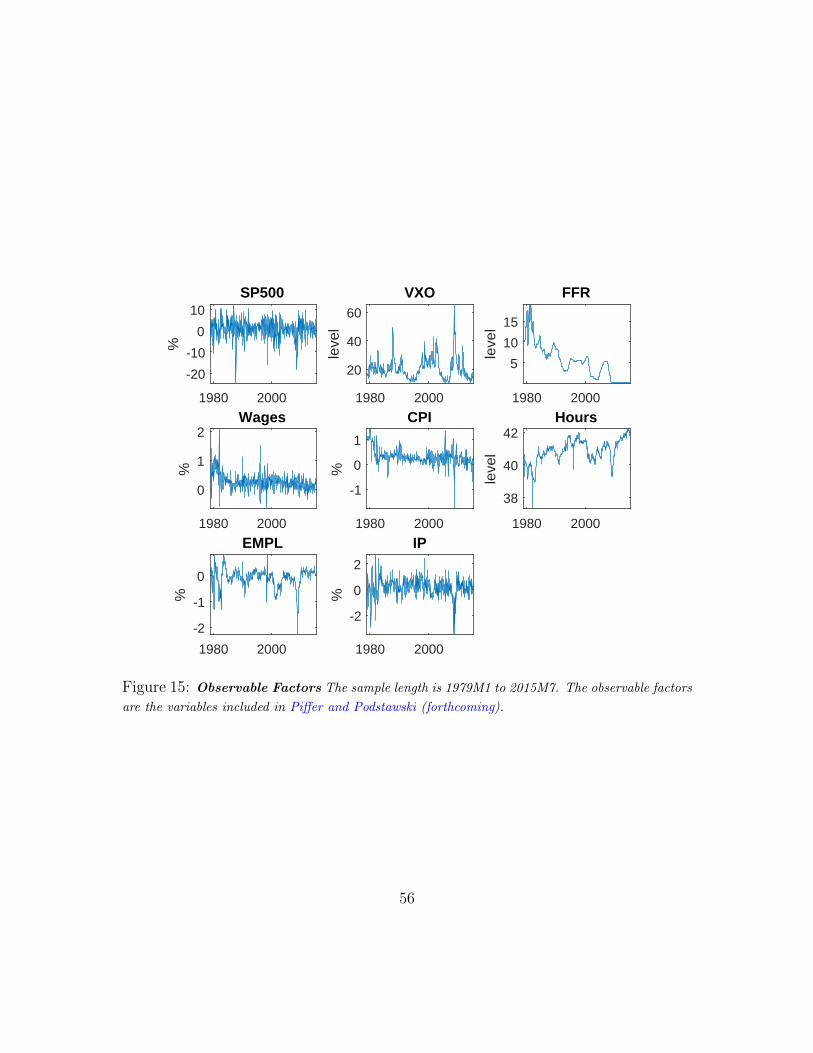
1980 2000

-20

-10

0

10

%

SP500

1980 2000

20

40

60

leve

l

VXO

1980 2000

5

10

15

leve

l

FFR

1980 2000

0

1

2

%

Wages

1980 2000

-1

0

1

%

CPI

1980 2000

38

40

42

leve

l

Hours

1980 2000

-2

-1

0

%

EMPL

1980 2000

-2

0

2

%

IP

Figure 15: Observable Factors The sample length is 1979M1 to 2015M7. The observable factors

are the variables included in Piffer and Podstawski (forthcoming).

56

1960 1970 1980 1990 2000 2010

-2

0

2

4

6

8

10

12

14

16

18

Policy Rate

Figure 16: Shadow Rate: Wu and Xia (2016) shadow rate available from 1960M1to 2015M11.

57