Remote Sens. 2020, 12, 433; doi:10.3390/rs12030433  www.mdpi.com/journal/remotesensing 

Article 

Combining Historical Remote Sensing, Digital Soil 

Mapping and Hydrological Modelling to Produce 

Solutions for Infrastructure Damage in Cosmo City, 

South Africa 

George van Zijl 1,*, Johan van Tol 2, Darren Bouwer 3, Simon Lorentz 4 and Pieter le Roux 3 

1  Unit for Environmental Sciences and Management, North‐West University,   

Potchefstroom 2520, South Africa 2  University of the Free State, Nelson Mandela Avenue, Bloemfontein 9301, South Africa; vantoljj@ufs.ac.za 3  Digital Soils Africa, 2 Alabaster street, Port Elizabeth 6001, South Africa; darren@dsafrica.co.za (D.B.); 

pieter@dsafrica.co.za (P.L.R.) 4  Centre for Water Resources Research, Univ. of Kwa‐Zulu‐Natal, Pietermaritzburg 3200, South Africa; 

slorentz@srk.co.za 

*  Correspondence: george.vanzijl@nwu.ac.za; Tel.: +27 18 299 2335 

Received: 13 December 2019; Accepted: 19 January 2020; Published: 29 January 2020 

Abstract: Urbanization and hydrology have an interactive relationship, as urbanization changing 

the  hydrology  of  a  system  and  the  hydrology  commonly  causing  structural  damage  to  the 

infrastructure. Hydrological modelling  has  been  used  to  quantify  the water  causing  structural 

impacts, and to provide solutions to the issues. However, in already‐urbanized areas, creating a soil 

map to use as input in the modelling process is difficult, as observation positions are limited and 

visuals of the natural vegetation which indicate soil distribution are unnatural. This project used 

historical satellite images in combination with terrain parameters and digital soil mapping methods 

to produce an accurate (Kappa statistic = 0.81) hydropedology soil map for the Cosmo City suburb 

in  Johannesburg,  South Africa.  The map was  used  as  input  into  the HYDRUS  2D  and  SWAT 

hydrological models to quantify the water creating road damage at Kampala Crescent, a road within 

Cosmo City (using HYDRUS 2D), as well as the impact of urbanization on the hydrology of the area 

(using  SWAT). HYDRUS  2D modelling  showed  that  a  subsurface  drain  installed  at  Kampala 

Crescent would need a carrying capacity of 0.3 m3.h−1.m−1 to alleviate the road damage, while SWAT 

modelling  shows  that  surface  runoff  in Cosmo City will  commence with  as  little  rainfall  as  2 

mm.month−1. This project showcases the value of multidisciplinary work. The remote sensing was 

invaluable to the mapping, which informed the hydrological modelling and subsequently provided 

answers to the engineers, who could then mitigate the hydrology‐related issues within Cosmo City. 

Keywords: urban soils; hydropedology; MNLR; machine learning; Johannesburg; remote sensing 

 

1. Introduction 

Urban  sprawl  is  set  to  continually  put  larger  developmental  pressure  on  our  natural  eco‐

systems, as larger portions of the world’s increasing population will live in cities. Currently, 54% of 

the world’s population are city dwellers, and this is projected to increase to 66% by 2050 [1], leading 

to a greater need for infrastructure development in the areas surrounding cities. 

The  relationship  between  hydrology  and  infrastructure  development  is  interactive.  The 

expansion of urban areas can  lead  to drastic changes  in hydrological processes. For example,  the 

generation mechanisms, magnitude, and timing of streamflow could be altered by infrastructure [2–

Remote Sens. 2020, 12, 433  2  of  18 

4]. On the other hand, these changes in hydrological processes can lead to infrastructural damages 

when they exceed construction thresholds [5,6]. Lately, the focus in urban development has been on 

water‐sensitive design strategies, which not only aim to protect infrastructure from water damage, 

but  also  limit  the  occurrence  of  flood  events,  while  striving  to  maintain  pre‐development 

hydrological dynamics [7]. In order to implement water‐sensitive design strategies, the hydrological 

processes before development should be identified, characterized, and quantified. 

The  study  of  water  movement  in  soils,  or  hydropedology  [8],  utilizes  soil  properties  to 

characterize the hydrological behavior within the soils. This is possible because water is a primary 

agent  in soil genesis, and directly  influences  the  formation of soil properties, which  in  turn carry 

unique  signatures  as  to  how  they  are  formed  [9–11].  Conversely,  hydrological  processes  are 

significantly influenced by the spatial distribution of soil properties [12], as soil transmits, stores, and 

reacts with water [13]. 

To capture the spatial distribution of soil properties, hydropedological studies generally use soil 

maps  [14,15]. However,  in  urban  areas  that  are  already  developed,  conventional  soil maps  are 

impossible to create due to the limited access to undisturbed soil observation positions. Therefore, 

older developments have double disadvantages, firstly by not being developed in a water‐sensitive 

way, and secondly, when hydrology‐related problems present themselves, the conventional methods 

to create a soil map for a hydropedological study are impossible to carry out. Digital soil mapping 

(DSM; [16]) provides the answer, as it uses environmental covariates (digital elevation models and 

satellite images) to predict the soil distribution at unobserved areas, based on the observed soils and 

their relation to the covariates. 

This paper presents how historical remote sensing was used to provide the pre‐urban land cover 

required to use DSM methods to create a soil map for Cosmo City, a suburb in Johannesburg, South 

Africa. By using Landsat satellite imagery from 2004, before the development commenced, a natural‐

conditions soil map could be created using DSM methodology. This map was then used as input to 

model  the  hydrology  of  the  suburb,  which  allowed  for  the  identification  and  prescription  of 

mitigation measures at Kampala Crescent—a road where subsoil water caused serious road damage. 

Furthermore,  the  influence  of  the  infrastructure development  on  the  hydrology  of  the  area was 

quantified by hydrological modelling of the entire suburb. This study differs from previous studies 

which used remote sensing data for hydrological models [17–19], as the Landsat images were used 

to map the soil, which were the input into the hydrological model, rather than using Landsat images 

for land cover or surface sealing indications. 

2. Materials and Methods 

2.1. Site Description 

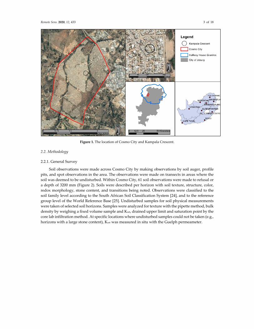
The study site consisted of Cosmo City, a suburb of Johannesburg (Figure 1), where construction 

started  in 2005. The geology of the study site is granite and gneiss of the Halfway House Granite 

formation [20], wherein Leptosols, Stagnosols, and Acrisols are the main soil reference groups found 

[21]. The natural vegetation is the Egoli Granite Grassland [22], however, very little of the natural 

vegetation remains with the construction of Cosmo City. Topographically, the study site lies on the 

Highveld of Southern Africa, at heights above sea level between 1400 m and 1540 m [23]. The terrain 

is hilly, with slopes of up to 12%, but with the majority of hillslopes having an average slope of below 

5%.  Johannesburg’s  climate  is  typical of  the  subtropical highland, with hot days during  summer 

(average  maximum  temperature  =  25  °C)  and  cold  nights  during  winter  (average  minimum 

temperature = 4 °C). The mean annual precipitation is 713 mm, mostly from thundershowers during 

the summer months. 

Remote Sens. 2020, 12, 433  3  of  18 

 

Figure 1. The location of Cosmo City and Kampala Crescent. 

2.2. Methodology 

2.2.1. General Survey 

Soil observations were made across Cosmo City by making observations by soil auger, profile 

pits, and spot observations in the area. The observations were made on transects in areas where the 

soil was deemed to be undisturbed. Within Cosmo City, 61 soil observations were made to refusal or 

a depth of 3200 mm (Figure 2). Soils were described per horizon with soil texture, structure, color, 

redox morphology, stone content, and transitions being noted. Observations were classified to the 

soil family level according to the South African Soil Classification System [24], and to the reference 

group level of the World Reference Base [25]. Undisturbed samples for soil physical measurements 

were taken of selected soil horizons. Samples were analyzed for texture with the pipette method, bulk 

density by weighing a fixed volume sample and Ksat, drained upper limit and saturation point by the 

core lab infiltration method. At specific locations where undisturbed samples could not be taken (e.g., 

horizons with a large stone content), Ksat was measured in situ with the Guelph permeameter. 

Remote Sens. 2020, 12, 433  4  of  18 

 

Figure 2. Soil observations for the Cosmo City soil observation database. 

2.2.2. Digital Soil Mapping 

To  create a  soil map, environmental  covariates were  collected  for  the  entire Halfway House 

Granite area, to use as ancillary variables in the mapping process. These layers included wet and dry 

season Landsat 5  images  [26],  taken on 10 April 2004  (wet season) and 31  July 2004  (dry season) 

respectively, before construction on Cosmo City began, and  the 30 m SRTM DEM  [26]. Covariate 

layers were resampled to have the same grid extent at a resolution of 30 m. Secondary covariate layers 

were derived from the Landsat 5 and DEM layers in SAGA‐GIS [27], which included: slope, profile 

curvature, planform curvature, aspect, topographic wetness index, flow accumulation, altitude above 

channel network, relative slope position, and multi resolution index of valley bottom flatness. From 

the wet  and dry  season  satellite  images  the normalized difference vegetation  index  (NDVI) was 

derived. 

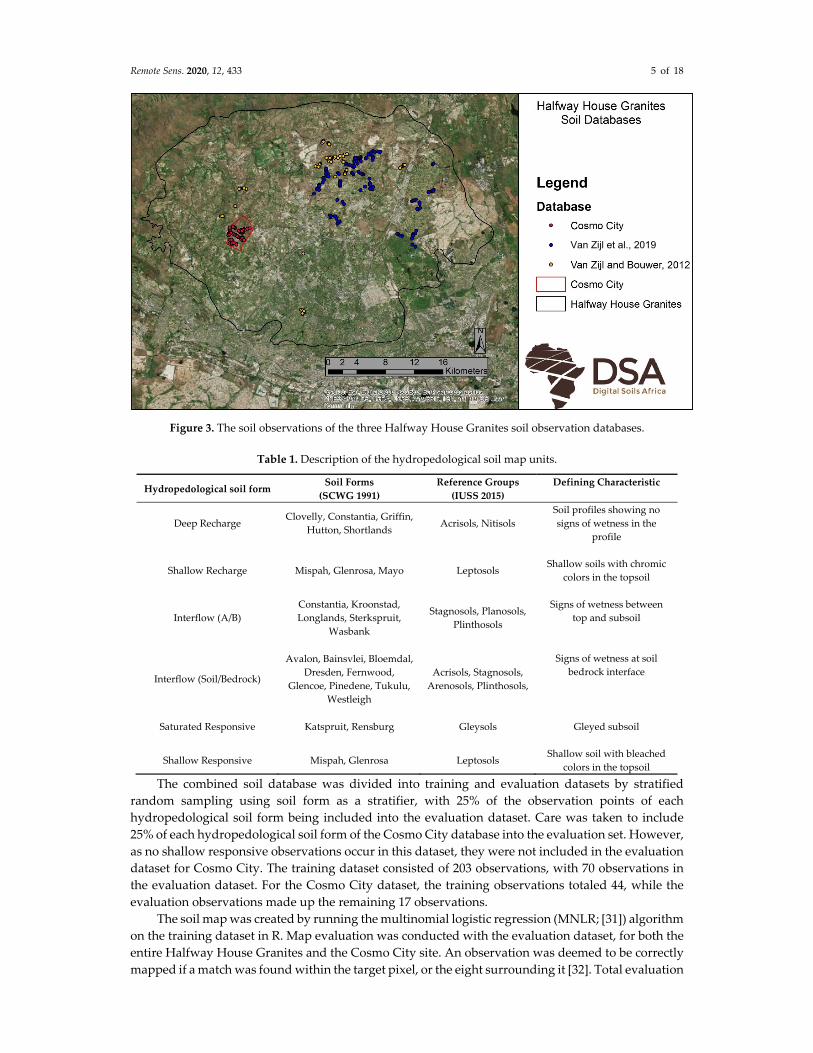
For modelling purposes the Cosmo City soil observation database was combined with two other 

soil observation databases within the Halfway House Granites (Figure 3) [28,29]. This allowed for the 

soil observation database to be enlarged with 212 observations (70 from Van Zijl and Bouwer 2012 

[29] and 142 from Van Zijl et al. (2019)) [28]. Therefore, the final Halfway House Granites database 

consisted of 273 soil observation points. Hydropedological soil forms [30] were derived from the soil 

form classifications according to Table 1. 

Remote Sens. 2020, 12, 433  5  of  18 

 

Figure 3. The soil observations of the three Halfway House Granites soil observation databases. 

Table 1. Description of the hydropedological soil map units. 

Hydropedological soil form Soil Forms 

(SCWG 1991) 

Reference Groups 

(IUSS 2015) 

Defining Characteristic 

Deep Recharge Clovelly, Constantia, Griffin, 

Hutton, Shortlands Acrisols, Nitisols 

Soil profiles showing no 

signs of wetness in the 

profile        

Shallow Recharge  Mispah, Glenrosa, Mayo  Leptosols Shallow soils with chromic 

colors in the topsoil        

Interflow (A/B) 

Constantia, Kroonstad, 

Longlands, Sterkspruit, 

Wasbank 

Stagnosols, Planosols, 

Plinthosols 

Signs of wetness between 

top and subsoil 

       

Interflow (Soil/Bedrock) 

Avalon, Bainsvlei, Bloemdal, 

Dresden, Fernwood, 

Glencoe, Pinedene, Tukulu, 

Westleigh 

Acrisols, Stagnosols, 

Arenosols, Plinthosols, 

Signs of wetness at soil 

bedrock interface 

       

Saturated Responsive  Katspruit, Rensburg  Gleysols  Gleyed subsoil        

Shallow Responsive  Mispah, Glenrosa  Leptosols Shallow soil with bleached 

colors in the topsoil 

The  combined  soil database was divided  into  training  and  evaluation datasets  by  stratified 

random  sampling  using  soil  form  as  a  stratifier,  with  25%  of  the  observation  points  of  each 

hydropedological soil  form being  included  into  the evaluation dataset. Care was  taken  to  include 

25% of each hydropedological soil form of the Cosmo City database into the evaluation set. However, 

as no shallow responsive observations occur in this dataset, they were not included in the evaluation 

dataset for Cosmo City. The training dataset consisted of 203 observations, with 70 observations in 

the evaluation dataset. For the Cosmo City dataset, the training observations totaled 44, while the 

evaluation observations made up the remaining 17 observations. 

The soil map was created by running the multinomial logistic regression (MNLR; [31]) algorithm 

on the training dataset in R. Map evaluation was conducted with the evaluation dataset, for both the 

entire Halfway House Granites and the Cosmo City site. An observation was deemed to be correctly 

mapped if a match was found within the target pixel, or the eight surrounding it [32]. Total evaluation 

Van Zijl et al., 2019

Remote Sens. 2020, 12, 433  6  of  18 

point accuracy, user’s and producer’s accuracy, and the Kappa coefficient were determined for the 

evaluation dataset to measure whether  the map was an acceptable representation of reality. Total 

evaluation  point  accuracy  is  the  total  number  of  observations  correctly mapped,  expressed  as  a 

percentage of the total number of evaluation observations. The user’s accuracy reflects the accuracy 

of the map from the user’s perspective. It is the number of evaluation observations correctly mapped 

within a specific map unit, expressed as a percentage of the total number of observations found on 

that specific map unit. The producer’s accuracy reflects the accuracy of a map from the producer’s 

perspective. It  is the number of evaluation observations within a specific class that were correctly 

mapped, expressed as a percentage of the total number of observations within that specific class. The 

Kappa  coefficient  represents  how  well  the  map  reflects  reality  when  compared  to  a  random 

designation of mapping units. Kappa coefficient values range between 0 and 1, with values close to 

0 indicating that the map is equal to a random designation and values close to 1 indicating that the 

map represents reality significantly better than a random designation would. 

2.2.3. Hydrological Modelling 

Kampala Crescent 

The lateral fluxes of Kampala Crescent were quantified in Hydrus 2‐D v 2.05 [33]. The location 

of the hillslope together with the conceptual hydrological response model created from the DSM soil 

map is presented in Figure 4. The material distribution reflects the distribution of the different soil 

horizons according to the South African soil classification system [24], as presented in the conceptual 

model.  The  soil  hydraulic  properties,  measured  in  the  laboratory  or  in  situ  with  the  Guelph 

permeameter for the different soil horizons, are presented in Table 2 together with the Van Genuchten 

parameters  estimated  from  the  hydraulic  properties  using  Rosetta  [34].  For  the  simulation,  the 

hillslope was first saturated through a zero‐pressure head at the surface for 10 days and then reduced 

to –400 mm for 30 days until seepage from the seepage face at Kampala Crescent ceased. A rain event 

was simulated by applying 1 day of zero pressure on the surface. Thereafter, the boundary condition 

at the surface was changed to an “Atmospheric Boundary”, with 6 mm.day−1 of potential evaporation 

from the surface. 

 

Figure 4. The conceptual hydrological response model for the Kampala Crescent hillslope. 

Remote Sens. 2020, 12, 433  7  of  18 

Table 2. Hydraulic properties and Van Genuchten parameters of dominant soil horizons used in Hydrus simulations. 

  Hydraulic Properties    Van Genuchten Parameters 

Horizon  Db  FC  DUL  Θs  Ks  Sand  Silt  Clay    Θr  Θs  Alpha  n  Ks  lambda   g.cm−3  mm.mm−1  mm.mm−1  mm.mm−1  mm.h−1  %  %  %               

Orthic A  1.39  0.2  0.22  0.477  237.2  67.6  11  22    0.1  0.44  0.00315  1.4802  237  0.5 

Red Apedal  1.42  0.22  0.24  0.464  73.9  56.6  15  29    0.1  0.43  0.00294  1.4273  73.9  0.5 

Soft Plinthic  1.55  0.27  0.35  0.416  2  39.7  14  46    0.1  0.42  0.00216  1.2054  4.1  0.5 

Gleyic  1.55  0.27  0.35  0.416  1  27.6  20  53    0.1  0.41  0.00231  1.2042  1.2  0.5 

Lithic  1.26  0.09  0.28  0.526  65.7  55.4  14  31    0.1  0.49  0.00271  1.3588  65.7  0.5 

Saprolite/Bed rock                    0.1  0.26  0.00258  1.1497  0.1  0.5 

Hydraulic Properties  Van Genuchten Parameters 

Db: Bulk density  Θr: Residual water content 

FC: Field Capacity  Θs: Saturated water content   

DUL: Drained Upper Limit  Alpha: inverse of air entry 

Θs: Saturated water content  n: pore size distribution 

Ks: Saturated hydrologic conductivity  Ks: Saturated hydrologic conductivity   

  lambda: Constant 

 

Remote Sens. 2020, 12, 433  8  of  18 

Cosmo City 

The effect of urbanization on the hydrology of the Cosmo City area was simulated using the Soil 

& Water Assessment Tool (SWAT). The SWAT is a widely used small watershed‐to‐river‐basin‐scale 

model. It is typically used to simulate the quality and quantity of surface and ground water and to 

predict the environmental impact of land use, land management practices, and climate change. Here 

we used QSWAT+ (version 0.9). 

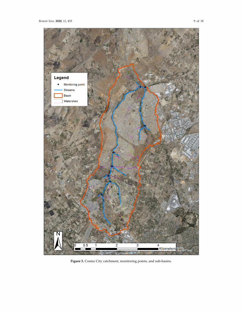
The catchment area was determined from a 30 m DEM and subdivided into nine sub‐basins, 

each with their own monitoring points (Figure 5). The current land use was obtained from the 2013–

2014 SA National Land‐Cover Map dataset [35]. The  land‐cover was re‐grouped  into SWAT land‐

uses with pre‐defined parameters for each use (Figure 6a). For the historic (before urbanization), we 

reclassified the urban areas to “grassland” and used the associated parameters. Soil information was 

obtained from the hydropedological survey (Figure 6b). Hydraulic parameters were derived from in 

situ and laboratory measurements (Table Error! Reference source not found.3). 

A nine‐year simulation period was selected (1 August 2003–31 December 2012). Climatic data 

for this period was obtained from the Climate Forecast System Reanalysis [36] project done by the 

National Center  for Environmental Prediction  (NCEP). WeatherGen  in SWAT+ Editor used daily 

precipitation,  temperature  (minimum  and maximum), wind  speed,  solar  radiation,  and  relative 

humidity  from  sta2607s2781e  (lat.  −25.76,  lon.  27.50)  to  generate  daily  climatic  variables  for  the 

simulations. Figure 7 presents the average monthly minimum and maximum temperatures as well 

as the total monthly rainfall for the simulation period. Results are reported from January 2004, which 

allowed the model 5 months to settle. 

Remote Sens. 2020, 12, 433  9  of  18 

 

Figure 5. Cosmo City catchment, monitoring points, and sub‐basins. 

Remote Sens. 2020, 12, 433  10  of  18 

 

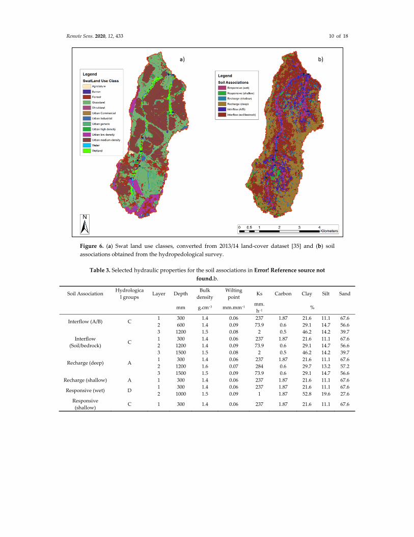
Figure  6.  (a)  Swat  land  use  classes,  converted  from  2013/14  land‐cover  dataset  [35]  and  (b)  soil 

associations obtained from the hydropedological survey. 

Table 3. Selected hydraulic properties for the soil associations in Error! Reference source not 

found.b. 

Soil Association Hydrologica

l groups Layer  Depth 

Bulk 

density 

Wilting 

point Ks  Carbon  Clay  Silt  Sand 

      mm  g.cm−3  mm.mm−1 mm.

h−1 % 

Interflow (A/B) 

  

C 

  

1  300  1.4  0.06  237  1.87  21.6  11.1  67.6 

2  600  1.4  0.09  73.9  0.6  29.1  14.7  56.6 

3  1200  1.5  0.08  2  0.5  46.2  14.2  39.7 

Interflow 

(Soil/bedrock) 

  

C 

  

1  300  1.4  0.06  237  1.87  21.6  11.1  67.6 

2  1200  1.4  0.09  73.9  0.6  29.1  14.7  56.6 

3  1500  1.5  0.08  2  0.5  46.2  14.2  39.7 

Recharge (deep) 

  

A 

  

1  300  1.4  0.06  237  1.87  21.6  11.1  67.6 

2  1200  1.6  0.07  284  0.6  29.7  13.2  57.2 

3  1500  1.5  0.09  73.9  0.6  29.1  14.7  56.6 

Recharge (shallow)  A  1  300  1.4  0.06  237  1.87  21.6  11.1  67.6 

Responsive (wet)   D  1  300  1.4  0.06  237  1.87  21.6  11.1  67.6 

2  1000  1.5  0.09  1  1.87  52.8  19.6  27.6 

Responsive 

(shallow) C  1  300  1.4  0.06  237  1.87  21.6  11.1  67.6 

Remote Sens. 2020, 12, 433  11  of  18 

 

Figure 7. Key climatic parameters used in the modelling (average monthly minimum and maximum 

temperatures and total monthly rainfall). 

3. Results and Discussion 

3.1. Digital Soil Mapping 

The Halfway House Granites hydropedological soil map (Figure 8) achieved an evaluation point 

accuracy of 80% and a Kappa statistic value of 0.71, indicating a substantial agreement with reality. 

These results are higher than expected, as lower accuracy was expected due to the urban environment 

mapped. The map should only be used in areas with a high observation density, such as Cosmo City. 

 

Figure 8. The hydropedological soil forms for the Halfway House Granites area. (SMU: Soil 

Mapping Unit) 

Remote Sens. 2020, 12, 433  12  of  18 

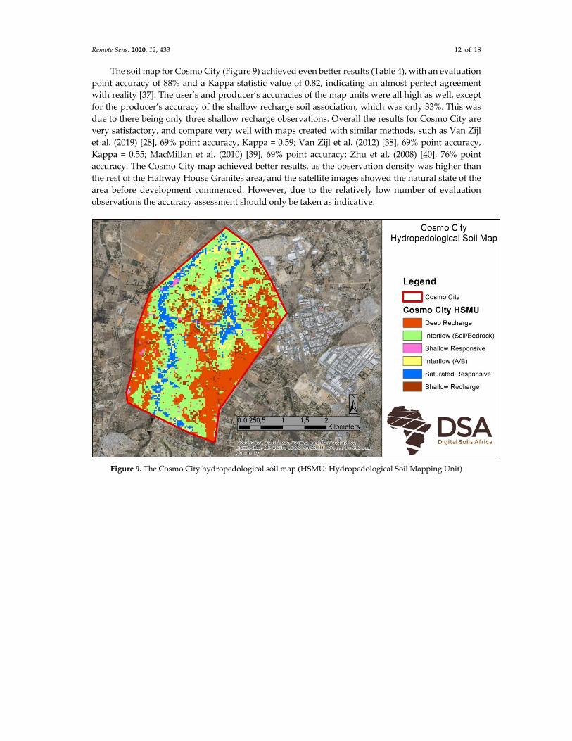
The soil map for Cosmo City (Figure 9) achieved even better results (Table 4), with an evaluation 

point accuracy of 88% and a Kappa statistic value of 0.82,  indicating an almost perfect agreement 

with reality [37]. The user’s and producer’s accuracies of the map units were all high as well, except 

for the producer’s accuracy of the shallow recharge soil association, which was only 33%. This was 

due to there being only three shallow recharge observations. Overall the results for Cosmo City are 

very satisfactory, and compare very well with maps created with similar methods, such as Van Zijl 

et al. (2019) [28], 69% point accuracy, Kappa = 0.59; Van Zijl et al. (2012) [38], 69% point accuracy, 

Kappa =  0.55; MacMillan  et al.  (2010)  [39],  69% point accuracy; Zhu  et al.  (2008)  [40], 76% point 

accuracy. The Cosmo City map achieved better results, as the observation density was higher than 

the rest of the Halfway House Granites area, and the satellite images showed the natural state of the 

area before development  commenced. However, due  to  the  relatively  low number of  evaluation 

observations the accuracy assessment should only be taken as indicative. 

 

Figure 9. The Cosmo City hydropedological soil map (HSMU: Hydropedological Soil Mapping Unit)

Remote Sens. 2020, 12, 433  13  of  18 

Table 4. Confusion matrix for the Cosmo City hydropedological soil map. 

    Users Accuracy       

    Deep 

Recharge 

Shallow 

Recharge 

Interflow 

(Soil/Bedrock) 

Interflow 

(A/B) 

Saturated 

Responsive Total  Correct  % Accuracy 

Producer’s Accuracy 

Deep Recharge  3          3  3  100 

Shallow 

Recharge 1  1  1      3  1  33 

Interflow 

(Soil/Bedrock)     8      8  8  100 

Interflow (A/B)        1    1  1  100 

Saturated 

Responsive         2  2  2  100 

  Total  4  1  9  1  2  17     

  Correct  3  1  8  1  2    15   

  % Accuracy  75  100  89  100  100      88 

Remote Sens. 2020, 12, 433  14  of  18 

3.2. Modelling Results 

3.2.1. Kampala Crescent 

The 2‐D simulations of Kampala crescent demonstrate that seepage will occur immediately after 

the rain event from the 9.3 m seepage face (Figure 10). The maximum seepage rate is approximately 

32 mm.h−1  and  occurs  after  6 h of  rain. The  seepage  rate will decline  as  a  6 mm.day−1 potential 

evaporation until seepage will cease after approximately 8 days. With a peak discharge rate of 32 

mm.h−1 the total volume of seepage water from in the area is approximately 0.3 m3.h‐1.m−1 of roadway 

(with the 9.3 m seepage face). If, for example, 100 m of Kampala Crescent is impacted by the seepage, 

subsurface drains should have a carrying capacity of 30 m3.h−1 (0.085 L.s−1.m−1). 

 

Figure 10. Resultant seepage hydrograph with one hour of rain at peak infiltration rate. 

3.2.2. Cosmo City 

The effect of urbanization on  the hydrology  is clearly  shown  in Figure 11, which  shows  the 

modelling results for the period from November 2011 to November 2012. The total streamflow from 

the Cosmo catchment  increased due  to the surface runoff also  increasing. This effect  is due to the 

surface  sealing  occurring with urbanization. Additionally,  the deep percolation  and  lateral  flow 

decreased  as  less water  infiltrated  the  soil.  Specifically  important  is  the  observation  that,  under 

natural conditions, surface flow was only initiated when monthly rainfall exceeded 50 mm.month−1. 

However,  after  urbanization  this  figure  dropped  to  2  mm.month−1.  This  impacts  storm  water 

management, as higher flow rates will occur, and they will also occur more frequently.

Remote Sens. 2020, 12, 433  15  of  18 

 

Figure 11. Average monthly modelling results for the Cosmo City suburb. (a) Streamflow, (b) Surface runoff, (c) Deep percolation, and (d) Lateral flow, for the time 

period November 2011 to November 2012. 

a b

c d

Remote Sens. 2020, 12, 433  16  of  18 

4. Conclusions 

Using  historical  satellite  images  from  before  the  Cosmo  City  suburb  was  developed,  and 

combining  these with DSM methods,  a  natural‐conditions  hydropedological  soil map  could  be 

created  for  the  suburb, with  a  Kappa  statistic  value  of  0.81.  This map  could  then  be  used  to 

parameterize both the HYDRUS and SWAT hydrological models. HYDRUS modelling was used to 

determine  the  source  and magnitude  of  soil water  causing  structural  damage  at  the  Kampala 

Crescent, and it was determined that a subsurface drain with a carrying capacity of 30 m3.h−1 (0.085 

L.s−1.m−1) should solve the problem. SWAT modelling revealed the effects of the development on the 

hydrology  of  the  area.  The  development  and  subsequent  surface  sealing  of  the  area  caused  an 

increase  in  runoff  and  streamflow,  but  reduced  the  evapotranspiration,  lateral  flow,  and  deep 

percolation.  The  hydrological  impacts  should  be  considered  when  designing  new  urban 

developments. 

This case study demonstrates the value of historic remote sensing data, as well as the power of 

multidisciplinary work. The  remote  sensing was  invaluable  to  the mapping, which  informed  the 

hydrological modelling, which provided  answers  to  the  engineers, who  could  then mitigate  the 

hydrology‐related issues within Cosmo City. 

Author Contributions: The authors made the following contributions to the work: Conceptualization, G.V.Z., 

D.B., S.L., J.V.T., and P.L.R.; Methodology, G.V.Z., D.B., S.L., J.V.T., and P.L.R., Data Acquisition, G.V.Z. and 

D.B., Formal Analysis, G.V.Z., D.B.,  S.L.  and  J.V.L.; Writing—Original Draft Preparation, G.V.Z.; Writing—

Review and Editing, J.V.T.; Project Administration, G.V.Z. and D.B., Funding Acquisition, G.V.Z., D.B., P.L.R., 

and J.V.L.. All authors have read and agreed to the published version of the manuscript. 

Funding: This study was funded by the Johannesburg Roads Agency. 

Acknowledgements: We would like to acknowledge the Johannesburg Roads Agency and Digital Soils Africa 

who allowed this data to be used for this publication 

Conflicts of Interest: The authors declare no conflicts of interest, and the funder played no role in the choice of 

research project; design of the study; in the collection, analyses, or interpretation of data; in the writing of the 

manuscript; or in the decision to publish the results. 

References 

1. United Nations Department  of  Economic  and  Social Affairs  (UN‐DESA),  Population Division. World 

Urbanization Prospects: The 2014 Revision; United Nations: New York, NY, USA, 2014. 

2. Walsh, C.J.; Roy, A.; Feminella, J.W.; Cottingham, P.; Groffman, P.M.; Morgan, R.P., II. The urban stream 

syndrome:  Current  knowledge  and  the  search  for  a  cure.  J.  N.  Am.  Benthol.  Soc.  2005,  24,  706–723, 

doi:10.1899/0887‐3593(2005)024\[0706: TUSSCK\]2.0.CO;2. 

3. Fox, D.M.; Witza, E.; Blanca, V.; Souliea, C.; Penalver‐Navarroa, M.; Dervieux, A. A case study of land cover 

change  (1950‐2003)  and  runoff  in  a  Mediterraean  catchment.  Appl.  Geogr.  2012,  32,  810–821, 

doi:10.1016/j.apgeog.2011.07.007. 

4. Dams, J.; Dujardin, J.; Reggers, R.; Bashir, I.; Canters, F.; Batelaan, O. Mapping impervious surface change 

from  remote  sensing  for  hydrological  modeling.  J.  Hydrol.  2013,  485,  84–95, 

doi:10.1016/j.jhydrol.2012.09.045. 

5. Toll, D.G.; Abedin, Z.; Buma, J.; Cui, Y.; Osman, A.S.; Phoon, K.K. The Impact of Changes in the Water Table 

and Soil Moisture on Structural Stability of Buildings and Foundation Systems: Systematic Review CEE10‐005 

(SR90); Technical Report; Collaboration for Environmental Evidence, Durham Research Online; Durham, 

United Kingdom, 2012. 

6. Dippenaar, M.A.; Van Rooy,  J.L. Vadose Zone Characterization  for Hydrogeological  and Geotechnical 

Application. In IAEG/AEG Annual Meeting Proceedings; Shakoor, A., Cato, K., Eds.; San Francisco, CA, USA, 

Springer International Publishing, 2019; Volume 2, doi:10.1007/978‐3‐319‐93127‐2_10. 

7. McGrane,  S.J.  Impacts  of  urbanisation  on  hydrological  and water  quality dynamics,  and  urban water 

management: A review, Hydrol. Sci. J. 2016, 61, 2295–2311, doi:10.1080/02626667.2015.1128084. 

8. Lin, H.S. Hydropedology: Bridging disciplines, scales, and data. Vadose Zone J. 2003, 2, 1–11. 

Remote Sens. 2020, 12, 433  17  of  18 

9. Ticehurst, J.L.; Cresswell, H.P.; Mckenzie, N.J.; Glover, M.R. Interpreting soil and topographic properties 

to conceptualize hillslope hydrology. Geoderma 2007, 137, 279–292. 

10. Van Tol, J.J.; Le Roux, P.A.L.; Hensley, M. Soil indicators of hillslope hydrology in Bedford catchment. S. 

Afr. J. Plant Soil 2010, 27, 242–251. 

11. Van  Tol,  J.J.;  Le  Roux,  P.A.L.;  Hensley, M.;  Lorentz,  S.A.  Soil  as  indicator  of  hillslope  hydrological 

behaviour in the Weatherley Catchment, Eastern Cape, South Africa. Water SA 2010, 36, 513–520. 

12. Lilly, A.; Boorman, D.B.; Hollis, J.M. The development of a hydrological classification of UK soils and the 

inherent scale changes. Nutr. Cycl. Agroecosys. 1998, 50, 299–302. 

13. Park, S.J.; McSweeney, K.; Lowery, B. Identification of the spatial distribution of soils using a 255 process‐

based terrain characterization. Geoderma 2001, 103, 249–272. 14. Van  Tol,  J.J.;  van  Zijl,  G.M.;  Riddell,  E.S.;  Fundisi,  D.  Application  of  hydropedological  insights  in 

hydrological modelling of the Stevenson Hamilton Research Supersite, Kruger National Park, South Africa. 

Water SA 2015, 41, 525–533. 15. Van Zijl, G.M.; Le Roux, P.A.L. Creating a hydrological soil map for the Stevenson Hamilton Supersite, 

Kruger National Park. Water SA 2014, 40, 331–336. 

16. McBratney, A.B.; Mendoça Santos, M.L.; Minasny, B. On digital soil mapping. Geoderma 2003, 117, 3–52. 

17. Mahiny, A.S.; Clarke, K.C. Simulating hydrologic impacts of urban growth using SLEUTH, multi criteria 

evaluation and runoff modelling. J. Environ. Inform. 2013, 22, 27–38. 

18. Ohana‐Levi, N.; Givati, A.; Alfasi, N.; Peeters, A.; Karnieli, A. Predicting  the effects of urbanization on 

runoff after frequent rainfall events. J. Land Use Sci. 2017, doi:10.1080/1747423X.2017.1385653. 

19. Chormanski, J.; Van de Voorde, T.; De Roeck, T.; Batelaan, O.; Canters, F. Improving Distributed Runoff 

Prediction in Urbanized Catchments with Remote Sensing based Estimates of Impervious Surface Cover. 

Sensors 2008, 8, 910–932, doi:10.3390/s8020910. 

20. Council for Geoscience. Geological Data 1:250 000; Council for Geoscience: Pretoria, South Africa, 2007. 

21. Land Type Survey Staff. Land Types of South Africa: Digital Map (1:250 000 Scale) and Soil Inventory Datasets; 

ARC‐Institute for Soil, Climate and Water: Pretoria, South Africa, 1972–2006. 

22. Mucina, L.; Rutherford, M.C. (Eds.) The Vegetation of South Africa, Lesotho and Swaziland; Strelitzia 19; South 

African National Biodiversity Institute: Pretoria, South Africa, 2006. 

23. Schulze, R.E. South African Atlas of Climatology and Agrohydrology; WRC Report 1489/1/06; Water research 

Commission: Pretoria, South Africa, 2007. 

24. Soil Classification Working Group. Soil Classification: A Taxonomic System for South Africa; Department of 

Agricultural Development: Pretoria, South Africa, 1991. 

25. IUSS Working Group WRB. World Reference  Base  for  Soil Resources  2014, Update  2015  International  Soil 

Classification System for Naming Soils and Creating Legends for Soil Maps; World Soil Resources Reports No. 

106; FAO: Rome, Italy, 2015. 

26. USGS  (United  States  Geological  Survey)  Landsat  images.  Available  online:  http://landsat.usgs.gov 

(accessed on 23 November 2018). 

27. Conrad, O.; Bechtel, B.; Bock, M.; Dietrich, H.; Fischer, E.; Gerlitz, L.; Wehberg, J.; Wichmann, V.; Boehner, 

J. System  for Automated Geoscientific Analyses  (SAGA) v. 2.1.4.Geosci. Model Dev. 2015, 8, 1991–2007, 

doi:10.5194/gmd‐8‐1991‐2015. 

28. Van Zijl, G.M.; Van Tol, J.J.; Tinnefeld, M.; Le Roux, P.A.L. A hillslope based digital soil mapping approach, 

for hydropedological assessments. Geoderma 2019, doi:10.1016/j.geoderma.2019.113888. 

29. Van Zijl, G.M.; Bouwer, D. Soil Observation Dataset from the Halfway House Granites; University of the Free 

State dataset; University of the Free State, Bloemfontein, South Africa, 2012. 

30. Van Tol,  J.J.; Lorentz, S.A. Hydropedological  interpretation of  soil distribution patterns  to  characterise 

groundwater/surface‐water interactions. Vadose Zone J. 2018, doi:10.2136/vzj2017.05.0097. 

31. Kempen, B.; Brus, D.J.; Heuvelink, G.B.M.; Stoorvogel, J.J. Updating the 1: 50 000 Dutch soil map using 

legacy soil data: A multinomial logistic regression approach. Geoderma 2009, 151, 311–326. 

32. Van Zijl, G.M.; Bouwer, D.; van Tol, J.J.; Le Roux, P.A.L. Functional digital soil mapping: A case study from 

Namarroi, Mozambique. Geoderma 2014, 219–220, 155–161. 

33. Šimůnek, J.; Van Genuchten, M.T.; Šejna, M. The HYDRUS Software Package for Simulating Two‐ and Three‐Dimensional Movement of Water, Heat, and Multiple Solutes  in Variably‐Saturated Media; Technical Manual, 

Version 1.0; PC Progress: Prague, Czech Republic, 2006. 

Remote Sens. 2020, 12, 433  18  of  18 

34. Schaap, M.G.; Leij, F.J.; van Genuchten, M.T. ROSETTA: A computer program for estimating soil hydraulic 

parameters with  hierarchical  pedotransfer  functions.  J.  Hydrol.  2001,  251,  163–176,  doi:10.1016/S0022‐

1694(01)00466‐8. 

35. Geoterraimage.  2013‐2014 South African National Land‐Cover Dataset; Report Created  for Department of 

Environmental Sciences; DEA/CARDNO SCPF002: Implementation of Land Use Maps for South Africa; 

Department of Environmental Affairs, Pretoria, South Africa. 2015; ©GEOTERRAIMAGE‐2014 

36. Saha, S.; Moorthi, S.; Pan, H.L.; Wu, X.; Wang, J.; Nadiga, S.; Tripp, P.; Kistler, R.; Woollen, J.; Behringer, D. 

et  al.  The  NCEP  Climate  Forecast  System  Reanalysis.  Bull.  Amer.  Meteor.  Soc.  2010,  91,  1015–1057, 

doi:10.1175/2010BAMS3001.1. 

37. Landis, J.R.; Koch, G.G. The measurement of observer agreement for categorical data. Biometrics 1977, 33, 

159–174, doi:10.2307/2529310. 

38. Van Zijl, G.M.; Le Roux, P.A.L.; Smith, H.J.C. 2012. Rapid soil mapping under restrictive conditions in Tete, 

Mozambique. In Digital Soil Assessments and Beyond; Minasny, B., Malone, B.P., McBratney, A.B., Eds.; CRC 

Press: Boca Raton, FL, USA, 335–339. 

39. MacMillan, R.A.; Moon, D.E.; Coupé; RA; Phillips, N. Predictive ecosystem mapping (PEM) for 8.2 million 

ha  of  forestland,  British  Columbia,  Canada.  In  Digital  Soil Mapping;  Bridging  Research,  Environmental 

Application and Operation; Boettinger, J.L., Howell, D.W., Moore, A.C., Hartemink, A.E., Kienast Brown, S., 

Eds.; Springer: Dordrecht, The Netherlands, 2010. 

40. Zhu, A.‐X.; Yang, L.; Li, B.; Qin, C.; English, E.; Burt,  J.E.; Zhou, C. Purposive sampling  for digital soil 

mapping for areas with limited data. In Digital Soil Mapping with Limited Data; Hartemink, A.E., McBratney, 

A.B., Mendonça‐Santos, M., Eds.; Springer: Dordrecht, The Netherlands, 2008. 

 

© 2020 by the authors. Licensee MDPI, Basel, Switzerland. This article is an open access 

article distributed under the terms and conditions of the Creative Commons Attribution 

(CC BY) license (http://creativecommons.org/licenses/by/4.0/).