Combining Predictive Densities using Nonlinear

Filtering with Applications to US Economics Data∗

Monica Billio † Roberto Casarin†

Francesco Ravazzolo‡ Herman K. van Dijk§∥∗∗

†University of Venice, GRETA Assoc. and School for Advanced Studies in Venice

‡Norges Bank

§Econometric Institute, Erasmus University Rotterdam

∥Department of Econometrics VU University Amsterdam and Tinbergen Institute

November 30, 2011

Abstract

We propose a multivariate combination approach to prediction based on

a distributional state space representation of the weights belonging to a set of

Bayesian predictive densities which have been obtained from alternative models.

Several specifications of multivariate time-varying weights are introduced with

a particular focus on weight dynamics driven by the past performance of the

predictive densities and the use of learning mechanisms. In the proposed

approach the model set can be incomplete, meaning that all models are

individually misspecified. The approach is assessed using statistical and

∗We benefited greatly from discussions with Frank Diebold, John Geweke and Frank Schorfheide.We also thank conference and seminar participants at: the 1st meeting of the European Seminar onBayesian Econometrics, the 4th CSDA International Conference on Computational and FinancialEconometrics, the 6th Eurostat Colloquium, Norges Bank, the NBER Summer Institute 2011Forecasting, the 2011 European Economic Association and Econometric Society and Universityof Pennsylvania for constructive comments on a preliminary version of the present paper. The viewsexpressed in this paper are our own and do not necessarily reflect those of Norges Bank.

∗∗Corresponding author: Herman K. van Dijk, hkvandijk@ese.eur.nl. Other contacts:billio@unive.it (Monica Billio); r.casarin@unive.it (Roberto Casarin); francesco.ravazzolo@norges-bank.no (Francesco Ravazzolo).

1

utility-based performance measures for evaluating density forecasts of US

macroeconomic time series and surveys of stock market prices. For the

macro series we find that incompleteness of the models is relatively large

in the 70’s, the beginning of the 80’s and during the recent financial crisis;

structural changes like the Great Moderation are empirically identified by

our model combination and the predicted probabilities of recession accurately

compare with the NBER business cycle dating. Model weights have substantial

uncertainty attached and neglecting this may seriously affect results. With

respect to returns of the S&P 500 series, we find that an investment strategy

using a combination of predictions from professional forecasters and from a

white noise model puts more weight on the white noise model in the beginning

of the 90’s and switches to giving more weight to the left tail of the professional

forecasts during the start of the financial crisis around 2008. Information on

the complete predictive distribution and not just on some moments turns out

to be very important in all investigated cases. More generally, the proposed

distributional state space representation offers a great flexibility in combining

densities.

JEL codes : C11, C15, C53, E37.

Keywords: Density Forecast Combination, Survey Forecast, Bayesian Filtering,

Sequential Monte Carlo.

1 Introduction

When multiple forecasts are available from different models or sources it is possible

to combine these in order to make use of all relevant information on the variable to

be predicted and, as a consequence, to possibly produce better forecasts. Most of the

literature on forecast combinations in economics and finance focus on point forecasts.

However forecasts value can be increased by supplementing point forecasts with some

2

measures of uncertainty. For example, interval and density forecasts are considered

important parts of the communication strategy from (central) banks to the public

and also for the decision-making process on financial asset allocation.

In the literature there is growing focus on model combination and many different

approaches are proposed. One of the first-mentioned papers on forecasting with

model combinations is Barnard [1963], who studied air passenger data, see also

Roberts [1965] who introduced a distribution which includes the predictions from two

experts (or models). This latter distribution is essentially a weighted average of the

posterior distributions of two models and is similar to the result of a Bayesian Model

Averaging (BMA) procedure. See Hoeting et al. [1999] for a review on BMA, with

an historical perspective. Raftery et al. [2005] and Sloughter et al. [2010] extend the

BMA framework by introducing a method for obtaining probabilistic forecasts from

ensembles in the form of predictive densities and apply it to weather forecasting. Our

paper builds on another stream of literature started with Bates and Granger [1969]

about combining predictions from different forecasting models. See Granger [2006]

for an updated review on forecast combination. Granger and Ramanathan [1984]

extend Bates and Granger [1969] and propose to combine forecasts with unrestricted

regression coefficients as weights. Liang et al. [2011] derive optimal weights in a

similar framework. Hansen [2007] and Hansen [2008] compute optimal weights by

maximizing a Mallow criterion. Terui and van Dijk [2002] generalize the least squares

model weights by representing the dynamic forecast combination as a state space. In

their work the weights are assumed to follow a random walk process. This approach

has been successfully extended by Guidolin and Timmermann [2009], who introduced

Markov-switching weights, and by Hoogerheide et al. [2010], who proposed robust

time-varying weights and accounted for both model and parameter uncertainty in

model averaging.

In the following, we assume that the weights associated with the predictive

3

densities are time-varying and propose a general distributional state-space

representation of predictive densities and of combination schemes. Our system allows

for all the models to be false and therefore the model set is misspecified as discussed

in Geweke [2010] and Amisano and Geweke [2010]. In this sense we extend the

state-space representation of Terui and van Dijk [2002] and Hoogerheide et al. [2010].

For a review on distributional state-space representation in the Bayesian literature,

see Harrison and West [1997]. We also extend model mixing via mixture of experts

(see for example Jordan and Jacobs [1994] and Huerta et al. [2003]) by allowing for

the possibility that all the models are misspecified. Our approach is general enough

to include multivariate linear and Gaussian models, dynamic mixtures and Markov-

switching models, as special cases. We represent our combination schemes in terms

of conditional densities and write equations for producing predictive densities and

not point forecasts (as is often the case) for the variables of interest. Accordingly to

this general representation we can estimate (optimal) model weights that maximize

general utility functions by taking into account past performances. In particular,

we consider convex combinations of the predictive densities and assume that the

time-varying weights associated with the different predictive densities belong to the

standard simplex. Under this constraint the weights can be interpreted as a discrete

probability distribution over the set of predictors. Tests for a specific hypothesis

on the values of the weights can be conducted due to their random nature. We

discuss weighting schemes with continuous dynamics, which allow for a smooth convex

combination of the prediction densities. A learning mechanism is also introduced to

allow the dynamics of each weight to be driven by the past and current performances

of the predictive densities in the combination scheme.

The constraint that time-varying weights associated with different forecast

densities belong to the standard simplex makes the inference process nontrivial

and calls for the use of nonlinear filtering methods. We apply simulation based

4

filtering methods, such as Sequential Monte Carlo (SMC), in the context of combining

forecasts, see for example Doucet et al. [2001] for a review with applications of

this approach and Del Moral [2004] for convergence issues. SMC methods are

extremely flexible algorithms that can be applied for inference to both off-line and

on-line analysis of nonlinear and non-Gaussian latent variable models, see for example

Creal [2009]. Billio and Casarin [2010] successfully applied SMC methods to time-

inhomogeneous Markov-switching models for an accurate forecasting of the business

cycle of the euro area.

To show practical and operational implications of the proposed approach, this

paper focuses on the problem of combining density forecasts from two relevant

economic datasets. The first one is given by density forecasts on two economic

time series: the quarterly series of US Gross Domestic Product (GDP) and US

inflation as measured by the Personal Consumption Expenditures (PCE) deflator.

The density forecasts are produced by several of the most commonly used models

in macroeconomics. We combine these densities forecasts in a multivariate set-

up with model and variable specific weights. For these macro series we find that

incompleteness of the models is relatively large in the 70’s, the beginning of the 80’s

and during the recent financial crisis; structural changes like the Great Moderation

are empirically identified by our model combination and the predicted probabilities

of recession accurately compare with the NBER business cycle dating. Model weights

have substantial uncertainty attached and neglecting this may seriously affect results.

To the best of our knowledge, there are no other papers applying this general density

combination method to macroeconomic data. The second dataset considers density

forecasts on the future movements of a stock price index. Recent literature has

shown that survey-based forecasts are particularly useful for macroeconomic variables,

but there are fewer results for finance. We consider density forecasts generated by

financial survey data. More precisely we use the Livingston dataset of six-months

5

ahead forecasts on the Standard & Poor’s 500, combine the survey-based densities

with the densities from a simple benchmark model and provide both statistical and

utility-based performance measures of the mixed combination strategy. To be specific,

with respect to the returns of the S&P 500 series we find that an investment strategy

using a combination of predictions from professional forecasters and from a white

noise model puts more weight on the white noise model in the beginning of the

90’s and switches to giving more weight to the left tail of the professional forecasts

during the start of the financial crisis around 2008. Information on the complete

predictive distribution and not just from basic first and second order moments turns

out to be very important in all investigated cases and more generally the proposed

distributional state-space representation of predictive densities and of combination

schemes demonstrates to be very flexible.

The structure of the paper is as follows. Section 2 describes the datasets and

introduces combinations of prediction densities in a multivariate context. Section

3 presents different models for the weights dynamics and introduces the learning

mechanism. In the Appendix alternative combination schemes and the relationships

with some existing schemes in the literature are briefly discussed. Section 4 describes

the nonlinear filtering problem and shows how Sequential Monte Carlo methods

could be used to combine prediction densities. Section 5 provides the results of the

application of the proposed combination method to the macroeconomic and financial

datasets. Section 6 concludes.

2 Data and Method

To motivate and show operational implications of our approach of combining

predictive densities, we start with an exploratory data analysis and subsequently

discuss our methodology.

6

2.1 Gross Domestic Product and Inflation

The first data set focuses on US GDP and US inflation. We collect quarterly

seasonally adjusted US GDP from 1960:Q1 to 2009:Q4 available from the US

Department of Commerce, Bureau of Economic Analysis (BEA). In a pseudo-real-time

out-of-sample forecasting exercise, we model and forecast the 1-step ahead quarterly

growth rate, 100(log(GDPt)− log(GDPt−1))1. For inflation we consider the quarterly

growth rate of the seasonally adjusted PCE deflator, 100(log(PCEt)− log(PCEt−1)),

from 1960:Q1 to 2009:Q4, also collected from the BEA website.

In forecasting we use an initial in-sample period from 1960:Q1 to 1969:Q4 to

obtain initial parameter estimates and we forecast GDP and PCE growth figures

for 1970:Q1. We then extend the estimation sample with the value in 1970:Q1, re-

estimating parameters, and forecast the next value for 1970:Q2. By iterating this

procedure up to the last value in the sample we end up with a total of 160 forecasts.

We consider K = 4 time series models which are widely applied to forecast

macroeconomic variables. Two models are linear specifications: an univariate

autoregressive model of order one (AR) and a bivariate vector autoregressive model

for GDP and PCE, of order one (VAR). We also apply two time-varying parameter

specifications: a two-state Markov-switching autoregressive model of order one

(ARMS) and a two-state Markov-switching vector autoregressive model of order one

for GDP and inflation (VARMS). We estimate models using Bayesian inference with

weak-informative conjugate priors and produce 1-step ahead predictive density via

direct simulations for AR and VAR, see, e.g. Koop [2003] for details; we use a Gibbs

sampling algorithm for ARMS and VARMS, see, e.g. Geweke and Amisano [2010]

for details. For both classes of models we simulate M = 1, 000 (independent) draws

to approximate the predictive likelihood of the GDP. Forecast combination practice

usually considers point forecasts, e.g. the median of the predictive densities (black

1We do not consider data revisions and use data from the 2010:Q1 vintage.

7

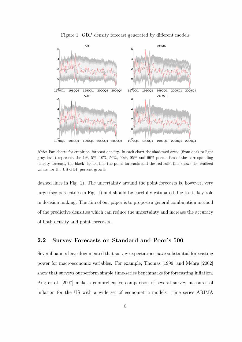
Figure 1: GDP density forecast generated by different models

1970Q1 1980Q1 1990Q1 2000Q1 2009Q4−2

0

2

4

6AR

1970Q1 1980Q1 1990Q1 2000Q1 2009Q4−2

0

2

4

6ARMS

1970Q1 1980Q1 1990Q1 2000Q1 2009Q4−2

0

2

4

6VAR

1970Q1 1980Q1 1990Q1 2000Q1 2009Q4−2

0

2

4

6VARMS

Note: Fan charts for empirical forecast density. In each chart the shadowed areas (from dark to light

gray level) represent the 1%, 5%, 10%, 50%, 90%, 95% and 99% percentiles of the corresponding

density forecast, the black dashed line the point forecasts and the red solid line shows the realized

values for the US GDP percent growth.

dashed lines in Fig. 1). The uncertainty around the point forecasts is, however, very

large (see percentiles in Fig. 1) and should be carefully estimated due to its key role

in decision making. The aim of our paper is to propose a general combination method

of the predictive densities which can reduce the uncertainty and increase the accuracy

of both density and point forecasts.

2.2 Survey Forecasts on Standard and Poor’s 500

Several papers have documented that survey expectations have substantial forecasting

power for macroeconomic variables. For example, Thomas [1999] and Mehra [2002]

show that surveys outperform simple time-series benchmarks for forecasting inflation.

Ang et al. [2007] make a comprehensive comparison of several survey measures of

inflation for the US with a wide set of econometric models: time series ARIMA

8

models, regressions using real activity measures motivated by the Phillips curve, and

term structure models. Results indicate that surveys outperform these methods in

point forecasting inflation.

The demand for forecasts for accurate financial variables has grown fast in recent

years due to several reasons, such as changing regulations, increased sophistication

of instruments, technological advances and recent global recessions. But compared

to macroeconomic applications, financial surveys are still rare and difficult to access.

Moreover, research on the properties of these databases such as their forecasting

power is almost absent. The exceptions are few and relate mainly to interest rates.

For example Fama and Gibbons [1984] compare term structure forecasts with the

Livingston survey and to particular derivative products; Lanne [2009] focuses on

economic binary options on the change in US non-farm payrolls.

We collect six month ahead forecasts for the Standard & Poor’s 500 (S&P 500)

stock price index from the Livingston survey.2 The Livingston Survey was started

in 1946 by the late columnist Joseph Livingston and it is the oldest continuous

survey of economists’ expectations. The Federal Reserve Bank of Philadelphia took

responsibility for the survey in 1990. The survey is conducted twice a year, in June and

December, and participants are asked different questions depending on the variable

of interest. Questions about future movements of stock prices were proposed to

participants from the first investigation made by Livingston in 1946, but the definition

of the variable and the base years have changed several times. Since the responsibility

passed to the Federal Reserve Bank of Philadelphia, questionnaires refer only to the

S&P500. So the first six month ahead forecast we have, with a small but reasonable

number of answers and a coherent index, is from December 1990 for June 1991.3

The last one is made in December 2009 for June 2010, for a total of 39 observations.

2See for data and documentation www.philadelphiafed.org/research-and-data/real-time-center/livingston-survey/

3The survey also contains twelve month ahead forecasts and from June 1992 one month aheadforecasts (just twice at year). We focus on six month ahead forecasts, which is the database withmore observations.

9

Figure 2: Livingston survey fan charts for the S&P 500. Left: survey data empiricaldensities. Right: nonparametric density estimates

1991M06 1995M12 2000M12 2005M12 2010M06

−30

−20

−10

0

10

20

30

40

1991M06 1995M12 2000M12 2005M12 2010M06

−30

−20

−10

0

10

20

30

40

Note: The shadowed areas (from dark to light gray level) and the horizontal lines represent the

1%, 5%, 10%, 50%, 90%, 95% and 99% percentiles of the corresponding density forecast and of the

sample distribution respectively, the black dashed line the point forecast and the red solid line shows

the realized values for S&P 500 percent log returns, for each out-of-sample observation. The dotted

black line shows the number of not-missing responses of the survey available at each date.

The surveys provide individual forecasts for the index value, we transform them in

percent log-returns using realized index values contained in the survey database, that

is yt+1,i = 100(log(pt+1,i) − log(pt)) with pt+1,i the forecast for the index value at

time t + 1 of individual i made at time t and pt the value of the index at time t

as reported in the database and given to participants at the time that the forecast

is made. Left chart in Figure 2 shows fan charts from the Livingston survey. The

forecast density is constructed by grouping all the responses at each period. The

number of survey forecasts can vary over time (black dotted line on the left chart);

the survey participants (units) may not respond and the unit identity can vary. A

problem of missing data can arise from both these situations. We do not deal with the

imputation problem because we are not interested in the single agent forecast process.

On the contrary, we consider the survey as an unbalanced panel and estimate over

time an aggregate predictive density. We account for the uncertainty in the empirical

10

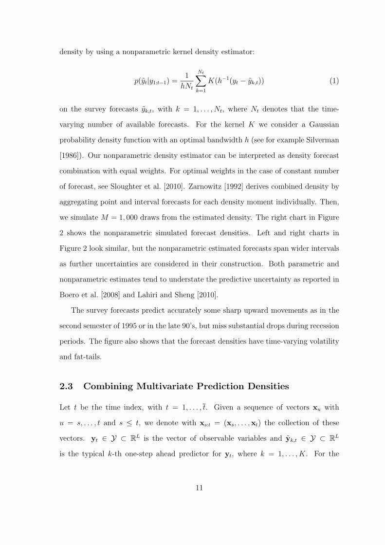
density by using a nonparametric kernel density estimator:

p(yt|y1:t−1) =1

hNt

Nt∑k=1

K(h−1(yt − yk,t)) (1)

on the survey forecasts yk,t, with k = 1, . . . , Nt, where Nt denotes that the time-

varying number of available forecasts. For the kernel K we consider a Gaussian

probability density function with an optimal bandwidth h (see for example Silverman

[1986]). Our nonparametric density estimator can be interpreted as density forecast

combination with equal weights. For optimal weights in the case of constant number

of forecast, see Sloughter et al. [2010]. Zarnowitz [1992] derives combined density by

aggregating point and interval forecasts for each density moment individually. Then,

we simulate M = 1, 000 draws from the estimated density. The right chart in Figure

2 shows the nonparametric simulated forecast densities. Left and right charts in

Figure 2 look similar, but the nonparametric estimated forecasts span wider intervals

as further uncertainties are considered in their construction. Both parametric and

nonparametric estimates tend to understate the predictive uncertainty as reported in

Boero et al. [2008] and Lahiri and Sheng [2010].

The survey forecasts predict accurately some sharp upward movements as in the

second semester of 1995 or in the late 90’s, but miss substantial drops during recession

periods. The figure also shows that the forecast densities have time-varying volatility

and fat-tails.

2.3 Combining Multivariate Prediction Densities

Let t be the time index, with t = 1, . . . , t. Given a sequence of vectors xu with

u = s, . . . , t and s ≤ t, we denote with xs:t = (xs, . . . ,xt) the collection of these

vectors. yt ∈ Y ⊂ RL is the vector of observable variables and yk,t ∈ Y ⊂ RL

is the typical k-th one-step ahead predictor for yt, where k = 1, . . . , K. For the

11

sake of simplicity we present the new combination method for the one-step ahead

forecasting horizon. The all methodology can be extended to multi-step ahead

forecasting horizons.

We assume that the vector of observable variables is generated from a distribution

with conditional density p(yt|y1:t−1) and that for each predictor yk,t there exists a

predictive density pk(yk,t|y1:t−1). To simplify the exposition, in what follows we define

yt = vec(Y ′t ), where Yt = (y1,t, . . . , yK,t) is the matrix with the predictors in the

columns and vec is the operator that stacks the columns of a matrix into a vector.

We denote with p(yt|y1:t−1) the joint predictive density of the set of predictors at

time t and let

p(y1:t|y1:t−1) =t∏

s=1

p(ys|y1:s−1)

be the joint predictive density of the predictors up to time t.

Generally speaking a combination scheme of a set of predictive densities is a

probabilistic relationship between the density of the observable variable and the set

of predictive densities. We assume that the relationship between the density of yt,

conditionally on y1:t−1, and the set of predictive densities from the K different sources

is the following:

p(yt|y1:t−1) =

∫YKt

p(yt|y1:t,y1:t−1)p(y1:t|y1:t−1)dy1:t (2)

where the dependence structure between the observable and the predictive is not

yet defined. This relationship might be misspecified because all the models are

false or the true DGP is a combination of unknown and unobserved models that

statistical and econometric tools can only partially approximate. In the following, to

model this possibly misspecified dependence between forecasting models, we consider

a parametric latent variable model. We also assume that the model is dynamic to

capture time variability in the dependence structure.

12

To define the latent variable model and the combination scheme we first introduce

the latent space. Let 1n = (1, . . . , 1)′ ∈ Rn and 0n = (0, . . . , 0)′ ∈ Rn be the n-

dimensional unit and null vectors respectively and denote with ∆[0,1]n ⊂ Rn the set of

all vectors w ∈ Rn such that w′1n = 1 and wk ≥ 0, k = 1, . . . , n. ∆[0,1]n is called the

standard n-dimensional simplex and is the latent space used in all our combination

schemes.

Secondly, we introduce the latent model, that is a matrix-valued stochastic

process, Wt ∈ W ⊂ RL × RKL, which represents the time-varying weights of the

combination scheme. Denote with wlh,t the h-th column and l-th row elements of Wt,

then we assume that the vectors wlt = (wl

1,t, . . . , wlKL,t)

′ satisfy wlt ∈ ∆[0,1]KL .

The definition of the latent space as the standard simplex and the consequent

restrictions on the dynamics of the weight process allow us to estimate a time

series of [0, 1] weights at time t − 1 when a forecast is made for yt. This latent

variable modelling framework generalizes previous literature on model combination

with exponential weights (see for example Hoogerheide et al. [2010]) by inferring

dynamics of positive weights which belong to the simplex ∆[0,1]LK .4 In such a way one

can interpret the weights as a discrete probability density over the set of predictors.

We assume that at time t, the time-varying weight process Wt has a distribution

with density p(Wt|y1:t−1, y1:t−1). Then we can write Eq. (2) as

p(yt|y1:t−1)=

∫YKt

(∫Wp(yt|Wt, yt)p(Wt|y1:t−1, y1:t−1)dWt

)p(y1:t|y1:t−1)dy1:t (3)

In the following, we assume that the time-varying weights have a first-order

Markovian dynamics and that they may depend on the past values y1:t−1 of the

predictors. According, the weights at time t have p(Wt|Wt−1, y1:t−1) as conditional

transition density. We usually assume that the weight dynamics depend on the recent

4Winkler [1981] does not restrict weights to the simplex, but allow them to be negative. It wouldbe interesting to investigate which restrictions are necessary to assure positive predictive densitieswith negative weights in our methodology. We leave this for further research.

13

values of the predictors, i.e.

p(Wt|Wt−1, y1:t−1) = p(Wt|Wt−1, yt−τ :t−1) (4)

with τ > 0.

Under these assumptions, the first integral in Eq. (3) is now defined on the set

YK(τ+1) and is taken with respect to a probability measure that has p(yt−τ :t|y1:t−1)

as joint predictive density. Moreover the conditional predictive density of Wt in Eq.

(3) can be further decomposed as follows

p(Wt|y1:t−1, y1:t−1)=

∫Wp(Wt|Wt−1, yt−τ :t−1)p(Wt−1|y1:t−2, y1:t−2)dWt−1

The above assumptions do not alter the general validity of the proposed approach

for the combination of the predictive densities. In fact, the proposed combination

method extends previous model pooling by assuming possibly non-Gaussian predictive

densities as well as nonlinear weights dynamics that maximize general utility

functions.

It is important to underline that this nonlinear state space representation offer

a great flexibility in combining densities. In example 1 we present a possible

specification of the conditional predictive density p(yt|Wt, yt), that we consider in

the applications.

In the appendix we present two further examples which allow for heavy-tailed

conditional distributions. In the next section we will also consider a specification for

the weights transition density p(Wt|Wt−1, y1:t−1).

Example 1 - (Gaussian combination scheme)

The conditional Gaussian combination model is defined by the probability density

14

function

p(yt|Wt, yt) ∝ exp

{−1

2(yt −Wtyt)

′Σ−1 (yt −Wtyt)

}(5)

where Wt ∈ ∆[0,1]L×KL is the weight matrix defined above and Σ is the covariance

matrix.�

A special case of the previous model is given by the following specification of the

combination

p(yt|Wt, yt)∝exp

{−1

2

(yt −

K∑k=1

wk,t ⊙ yk,t

)′

Σ−1

(yt −

K∑k=1

wk,t ⊙ yk,t

)}(6)

where wk,t = (w1k,t, . . . , w

Lk,t)

′ is a weights vector and ⊙ is the Hadamard’s product.

The system of weights is given as wlt = (wl

1,t, . . . , wlL,t)

′ ∈ ∆[0,1]L , for l = 1, . . . , L. In

this model the weights may vary over the elements of yt and only the i-th elements

of each predictor yk,t of yt are combined in order to have a prediction of the i-th

element of yt.

A more parsimonious model than the previous one is given by

p(yt|Wt, yt) ∝ exp

{−1

2

(yt −

K∑k=1

wk,tyk,t

)′

Σ−1

(yt −

K∑k=1

wk,tyk,t

)}(7)

where wt = (w1,t, . . . , wK,t)′ ∈ ∆[0,1]K . In this model all the elements of the prediction

yk,t given by the k-th model have the same weight, while the weights may vary across

the models.

3 Weight Dynamics

In this section we present some existing and new specifications of the conditional

density of the weights given in Eq. (4). In order to write the density of the

combination models in a more general and compact form, we introduce a vector

15

of latent processes xt = vec(Xt) ∈ RKL2where Xt = (x1

t , . . . ,xLt )

′ and xlt =

(xl1,t, . . . , xlKL,t)

′ ∈ X ⊂ RKL. Then, for the l-th predicted variables of the vector

yt, in order to have weights wlt which belong to the simplex ∆[0,1]K , we introduce the

multivariate transform g = (g1, . . . , gKL)′

g :

RKL → ∆[0,1]KL

xlt 7→ wt = (g1(x

lt), . . . , gKL(x

lt))

′(8)

Under this convexity constraint, the weights can be interpreted as a discrete

probability distribution over the set of predictors. A hypothesis on the specific values

of the weights can be tested by using their random distribution.

In the simple case of a constant-weights combination scheme the latent process

is simply xlh,t = xlh, ∀t, where xlh ∈ R is a set of predictor-specific parameters. The

weights can be written as: wlk = gk(x

l) for each l = 1, . . . , L, where

gh(xl) =

exp{xlh}∑KLj=1 exp{xlj}

, withh = 1, . . . , KL (9)

is the multivariate logistic transform. In standard Bayesian model averaging, xl

is equal to the marginal likelihood, see, e.g. Hoeting et al. [1999]. Geweke and

Whiteman [2006] propose to use the logarithm of the predictive likelihood, see, e.g.

Hoogerheide et al. [2010] for further details. Mitchell and Hall [2005] discuss the

relationship of the predictive likelihood to the Kullback-Leibler information criterion.

We note that such weights assume that the model set is complete and the true DGP

can be observed or approximated by a combination of different models.

3.1 Time-varying Weights

If parameters are estimated recursively over time then these estimates might vary

along the recursion. Thus following the same idea, which is underlying the recursive

16

least squares regression model, it is possible to replace the parameters xlh with a

stochastic process xlh,t which accounts for the time variation of the weight estimates

and assume the trivial dynamics xlh,t = xlh,t−1, ∀t and l = 1, . . . , L.

We generalize this simple time-varying weight scheme. In our first specification of

Wt, we assume that the weights have their own fluctuations generated by the latent

process

xt ∼ p(xt|xt−1) (10)

with a non-degenerate distribution and then apply the transform g defined in Eq. (8)

wlt = g(xl

t), l = 1, . . . , L (11)

where wlt = (wl

1,t, . . . , wlKL,t)

′ ∈ ∆[0,1]KL is the l-th row of Wt.

Example 1 - (Logistic-Transformed Gaussian Weights)

We assume that the conditional distribution of xt is a Gaussian one

p(xt|xt−1) ∝ exp

{−1

2(xt − xt−1)

′ Λ−1 (xt − xt−1)

}(12)

where Λ is the covariance matrix and the weights are logistic transforms of the latent

process

wlt =

exp{xlh}∑KLj=1 exp{xlj}

, withh = 1, . . . , KL

with l = 1, . . . , L.�

3.2 Learning Mechanism

We consider learning strategies based on the distribution of the forecast errors. More

precisely, we evaluate the past performance of each prediction model and compare it

with the performances of the other models.

17

The contribution of this section is to generalize the weight structures given in the

previous sections and related literature (see for example Hoogerheide et al. [2010]) by

including a learning strategy in the weight dynamics and by estimating, with nonlinear

filtering, the weight posterior probability. Therefore the weights are explicitly driven

by the past and current forecast errors and capture the residual evolution of the

combination scheme by the dynamic structure. Instead of choosing between the use

of exponential discounting in the weight dynamics or time-varying random weights

(see Diebold and Pauly [1987] and for an updated review Timmermann [2006]), we

combine the two approaches.

We consider an exponentially weighted moving average of the forecast errors

of the different predictors. In this way it is possible to have at the same time a

better estimate of the current distribution of the prediction error and to attribute

greater importance to the last prediction error. We consider a moving window of

τ observations and define the distance matrix Elt = (el,1t , . . . , e

l,Lt ), where el,dt =

(el,d1,t, . . . , el,dK,t)

′, with d = 1, . . . , L, is a vector of exponentially weighted average errors

el,dk,t = (1− λ)τ∑

i=1

λi−1(ylt−i − yl,dk,t−i)2 (13)

with λ ∈ (0, 1) a smoothing parameter and yl,dk,t−i is the point forecast at time t given

by model k for the variable ylt−i. Define et = vec(Et), where Et = (E1t , . . . , E

Lt ), then

we introduce the following weight model

wlt = g(xl

t), l = 1, . . . , L (14)

xt = zt − et (15)

zt = zt−1 (16)

18

where zt = vec(z1t , . . . , zLt ) and zlt ∈ RKL. The model can be rewritten as follows

wlt = g(xl

t), l = 1, . . . , L (17)

xt = xt−1 −∆et (18)

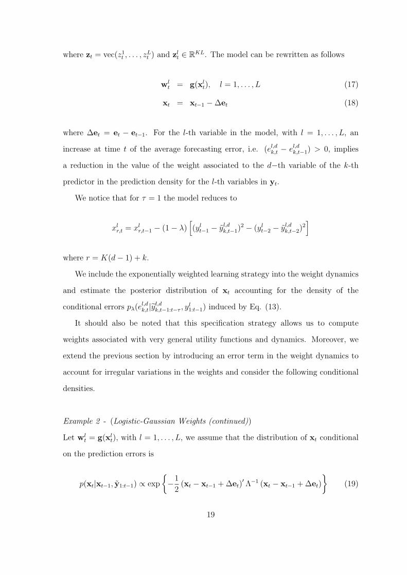
where ∆et = et − et−1. For the l-th variable in the model, with l = 1, . . . , L, an

increase at time t of the average forecasting error, i.e. (el,dk,t − el,dk,t−1) > 0, implies

a reduction in the value of the weight associated to the d−th variable of the k-th

predictor in the prediction density for the l-th variables in yt.

We notice that for τ = 1 the model reduces to

xlr,t = xlr,t−1 − (1− λ)[(ylt−1 − yl,dk,t−1)

2 − (ylt−2 − yl,dk,t−2)2]

where r = K(d− 1) + k.

We include the exponentially weighted learning strategy into the weight dynamics

and estimate the posterior distribution of xt accounting for the density of the

conditional errors pλ(el,dk,t|y

l,dk,t−1:t−τ , y

l1:t−1) induced by Eq. (13).

It should also be noted that this specification strategy allows us to compute

weights associated with very general utility functions and dynamics. Moreover, we

extend the previous section by introducing an error term in the weight dynamics to

account for irregular variations in the weights and consider the following conditional

densities.

Example 2 - (Logistic-Gaussian Weights (continued))

Let wlt = g(xl

t), with l = 1, . . . , L, we assume that the distribution of xt conditional

on the prediction errors is

p(xt|xt−1, y1:t−1) ∝ exp

{−1

2(xt − xt−1 +∆et)

′ Λ−1 (xt − xt−1 +∆et)

}(19)

19

�

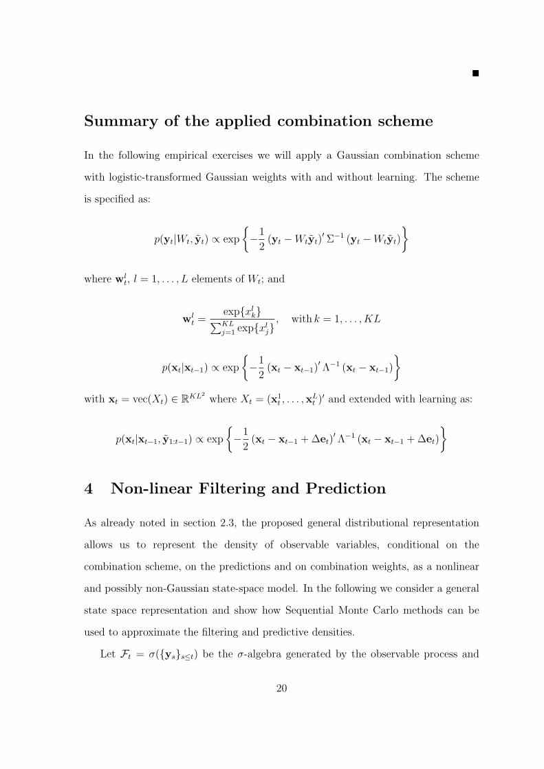
Summary of the applied combination scheme

In the following empirical exercises we will apply a Gaussian combination scheme

with logistic-transformed Gaussian weights with and without learning. The scheme

is specified as:

p(yt|Wt, yt) ∝ exp

{−1

2(yt −Wtyt)

′Σ−1 (yt −Wtyt)

}

where wlt, l = 1, . . . , L elements of Wt; and

wlt =

exp{xlk}∑KLj=1 exp{xlj}

, with k = 1, . . . , KL

p(xt|xt−1) ∝ exp

{−1

2(xt − xt−1)

′ Λ−1 (xt − xt−1)

}with xt = vec(Xt) ∈ RKL2

where Xt = (x1t , . . . ,x

Lt )

′ and extended with learning as:

p(xt|xt−1, y1:t−1) ∝ exp

{−1

2(xt − xt−1 +∆et)

′ Λ−1 (xt − xt−1 +∆et)

}

4 Non-linear Filtering and Prediction

As already noted in section 2.3, the proposed general distributional representation

allows us to represent the density of observable variables, conditional on the

combination scheme, on the predictions and on combination weights, as a nonlinear

and possibly non-Gaussian state-space model. In the following we consider a general

state space representation and show how Sequential Monte Carlo methods can be

used to approximate the filtering and predictive densities.

Let Ft = σ({ys}s≤t) be the σ-algebra generated by the observable process and

20

assume that the predictors yt = (y′1,t, . . . , y

′K,t)

′ ∈ Y ⊂ RKL stem from a Ft−1-

measurable stochastic process associated with the predictive densities of the K

different models in the pool. Let wt = (w′1,t, . . .w

′K,t)

′ ∈ X ⊂ RKL be the vector of

latent variables (i.e. the model weights) associated with yt and θ ∈ Θ the parameter

vector of the predictive model. Include the parameter vector into the state vector

and thus define the augmented state vector zt = (wt,θ) ∈ Y ×Θ. The distributional

state space form of the forecast model is

yt|zt, yt ∼ p(yt|zt, yt) (20)

zt|zt−1 ∼ p(zt|zt−1, y1:t−1) (21)

z0 ∼ p(z0) (22)

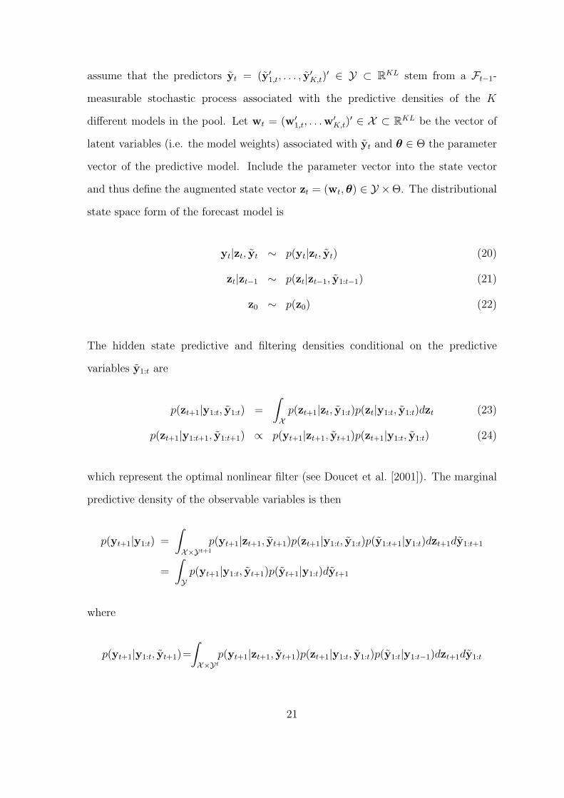
The hidden state predictive and filtering densities conditional on the predictive

variables y1:t are

p(zt+1|y1:t, y1:t) =

∫Xp(zt+1|zt, y1:t)p(zt|y1:t, y1:t)dzt (23)

p(zt+1|y1:t+1, y1:t+1) ∝ p(yt+1|zt+1, yt+1)p(zt+1|y1:t, y1:t) (24)

which represent the optimal nonlinear filter (see Doucet et al. [2001]). The marginal

predictive density of the observable variables is then

p(yt+1|y1:t) =

∫X×Yt+1

p(yt+1|zt+1, yt+1)p(zt+1|y1:t, y1:t)p(y1:t+1|y1:t)dzt+1dy1:t+1

=

∫Yp(yt+1|y1:t, yt+1)p(yt+1|y1:t)dyt+1

where

p(yt+1|y1:t, yt+1)=

∫X×Yt

p(yt+1|zt+1, yt+1)p(zt+1|y1:t, y1:t)p(y1:t|y1:t−1)dzt+1dy1:t

21

is the conditional predictive density of the observable given the predicted variables.

To construct an optimal nonlinear filter we have to implement the exact update

and prediction steps given above. As an analytical solution of the general filtering

and prediction problems is not known for non-linear state space models, we apply

an optimal numerical approximation method, that converges to the optimal filter

in Hilbert metric, in the total variation norm or in a weaker distance suitable for

random probability distributions (see Legland and Oudjane [2004]). More specifically

we consider a sequential Monte Carlo (SMC) approach to filtering. See Doucet et al.

[2001] for an introduction to SMC and Creal [2009] for a recent survey on SMC in

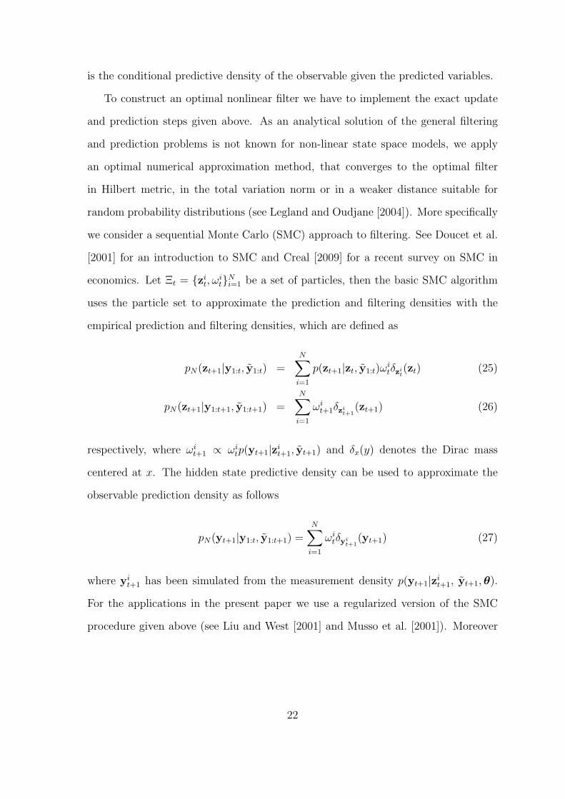
economics. Let Ξt = {zit, ωit}Ni=1 be a set of particles, then the basic SMC algorithm

uses the particle set to approximate the prediction and filtering densities with the

empirical prediction and filtering densities, which are defined as

pN(zt+1|y1:t, y1:t) =N∑i=1

p(zt+1|zt, y1:t)ωitδzit(zt) (25)

pN(zt+1|y1:t+1, y1:t+1) =N∑i=1

ωit+1δzit+1

(zt+1) (26)

respectively, where ωit+1 ∝ ωi

tp(yt+1|zit+1, yt+1) and δx(y) denotes the Dirac mass

centered at x. The hidden state predictive density can be used to approximate the

observable prediction density as follows

pN(yt+1|y1:t, y1:t+1) =N∑i=1

ωitδyi

t+1(yt+1) (27)

where yit+1 has been simulated from the measurement density p(yt+1|zit+1, yt+1,θ).

For the applications in the present paper we use a regularized version of the SMC

procedure given above (see Liu and West [2001] and Musso et al. [2001]). Moreover

22

we assume that the densities p(ys|y1:s−1) are discrete

p(ys|y1:s−1) =M∑j=1

δyjs(ys)

This assumption does not alter the validity of our approach and is mainly motivated

by the forecasting practice, see literature on model pooling, e.g. Jore et al. [2010]. In

fact, the predictions usually come from different models or sources. In some cases the

discrete prediction density is the result of a collection of point forecasts from many

subjects, such as surveys forecasts. In other cases the discrete predictive is a result

of a Monte Carlo approximation of the predictive density (e.g. Importance Sampling

or Markov-Chain Monte Carlo approximations).

Under this assumption it is possible to approximate the marginal predictive

density by the following steps. First, draw j independent values yj1:t+1, with

j = 1, . . . ,M from the sequence of predictive densities p(ys+1|y1:s), with s = 1, . . . , t.

Secondly, apply the SMC algorithm, conditionally on yj1:t+1, in order to generate the

particle set Ξi,jt = {zi,j1:t, ω

i,jt }Ni=1, with j = 1, . . . ,M . At the last step, simulate yi,j

t+1

from p(yt+1|zi,jt+1, yjt+1) and obtain the following empirical predictive density

pN,M(yt+1|y1:t) =1

M

M∑j=1

N∑i=1

ωi,jt δyi,j

t+1(yt+1) (28)

5 Empirical Applications

5.1 Comparing Combination Schemes

To shed light on the predictive ability of individual models, we consider several

evaluation statistics for point and density forecasts previously proposed in literature.

We compare point forecasts in terms of Root Mean Square Prediction Errors

23

(RMSPE)

RMSPEk =

√√√√ 1

t∗

t∑t=t

ek,t+1

where t∗ = t − t + 1 and ek,t+1 is the square prediction error of model k and test

for substantial differences between the AR benchmark and the model k by using the

Clark and West [2007]’ statics (CW). The null of the CW test is equal mean square

prediction errors, the one-side alternative is the superior predictive accuracy of the

model k.

Following Welch and Goyal [2008] we investigate how square prediction varies over

time by a graphical inspection of the Cumulative Squared Prediction Error Difference

(CSPED):

CSPEDk,t+1 =t∑

s=t

fk,s+1,

where fk,t+1 = eAR,t+1 − ek,t+1 with k =VAR, ARMS, VARMS. Increases in

CSPEDk,t+1 indicate that the alternative to the benchmark (AR model) predicts

better at out-of-sample observation t+ 1.

We evaluate the predictive densities using a test of absolute forecast accuracy.

As in Diebold et al. [1998], we utilize the Probability Integral Transforms (PITS),

of the realization of the variable with respect to the forecast densities. A forecast

density is preferred if the density is correctly calibrated, regardless of the forecasters

loss function. The PITS at time t+ 1 are:

PITSk,t+1 =

∫ yt+1

−∞p(uk,t+1|y1:t)duk,t+1.

and should be uniformly, independently and identically distributed if the forecast

densities p(yk,t+1|y1:t), for t = t, . . . , t, are correctly calibrated. Hence, calibration

evaluation requires the application of tests for goodness of fit. We apply the Berkowitz

[2001] test for zero mean, unit variance and independence of the PITS. The null of

24

the test is no calibration failure.

For our analysis of relative predictive accuracy, we consider a Kullback Leibler

Information Criterion (KLIC) based test, utilizing the expected difference in the

Logarithmic Scores of the candidate forecast densities; see for example Kitamura

[2002], Mitchell and Hall [2005], Amisano and Giacomini [2007], Kascha and

Ravazzolo [2010] and Caporin and Pres [2010]. Geweke and Amisano [2010] and

Mitchell and Wallis [2010] discuss the value of information-based methods for

evaluating forecast densities that are well calibrated on the basis of PITS tests. The

KLIC chooses the model which on average gives higher probability to events that have

actually occurred. Specifically, the KLIC distance between the true density p(yt+1|y1:t)

of a random variable yt+1 and some candidate density p(yk,t+1|y1:t) obtained from

model k is defined as

KLICk,t+1 =

∫p(yt+1|y1:t) ln

p(yt+1|y1:t)p(yk,t+1|y1:t)

dyt+1,

= Et[ln p(yt+1|y1:t)− ln p(yk,t+1|y1:t))]. (29)

where Et(·) = E(·|Ft) is the conditional expectation given information set Ft at

time t. An estimate can be obtained from the average of the sample information,

yt+1, . . . , yt+1, on p(yt+1|y1:t) and p(yk,t+1|y1:t):

KLICk =1

t∗

t∑t=t

[ln p(yt+1|y1:t)− ln p(yk,t+1|y1:t)]. (30)

Even though we do not know the true density, we can still compare multiple densities,

p(yk,t+1|y1:t). For the comparison of two competing models, it is sufficient to consider

the Logarithmic Score (LS), which corresponds to the latter term in the above sum,

LSk = − 1

t∗

t∑t=t

ln p(yk,t+1|y1:t), (31)

25

for all k and to choose the model for which the expression in (31) is minimal, or as

we report in our tables, the opposite of the expression in (31) is maximal. Differences

in KLIC can be statistically tested. We apply a test of equal accuracy of two density

forecasts for nested models similar to Mitchell and Hall [2005], Giacomini and White

[2006] and Amisano and Giacomini [2007]. For the two 1-step ahead density forecasts,

p(yAR,t+1|y1:t) and p(yk,t+1|y1:t) we consider the loss differential

dk,t+1 = ln p(yAR,t+1|y1:t)− ln p(yk,t+1|y1:t).

and apply the following Wald test:

GWk = t∗

(1

t∗

t∑t=t

hk,tdk,t+1

)′

Σk,t+1

(1

t∗

t∑t=t

hk,tdk,t+1

), (32)

where hk,t = (1, dk,t)′, and Σk,t+1 is the HAC estimator for the variance of (hk,tdk,t+1).

The null is of the test is equal predictability.

Analogous to our use of the CSPED for graphically examining relative MSPEs

over time, and following Kascha and Ravazzolo [2010], we define the Cumulative Log

Score Difference (CLSD):

CLSDk,t+1 = −t∑

s=t

dk,s+1, (33)

If CLSDk,t+1 increases at observation t+ 1, this indicates that the alternative to the

AR benchmark has a higher log score.

5.2 Application to GDP

First we evaluate the performance of the individual models for forecasting US GDP

growth. Results in Table 1 indicate that the linear models produce the most accurate

point and density forecasts. The left column of figure 3 shows that the predictive

26

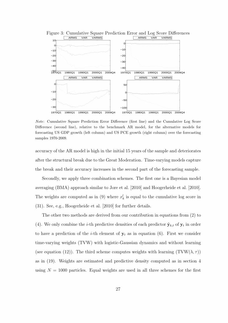
Figure 3: Cumulative Square Prediction Error and Log Score Differences

1970Q1 1980Q1 1990Q1 2000Q1 2009Q4−50

−40

−30

−20

−10

0

10

ARMS VAR VARMS

1970Q1 1980Q1 1990Q1 2000Q1 2009Q4

−40

−30

−20

−10

0

ARMS VAR VARMS

1970Q1 1980Q1 1990Q1 2000Q1 2009Q4

−30

−20

−10

0

ARMS VAR VARMS

1970Q1 1980Q1 1990Q1 2000Q1 2009Q4

−100

−50

0

50

ARMS VAR VARMS

Note: Cumulative Square Prediction Error Difference (first line) and the Cumulative Log Score

Difference (second line), relative to the benchmark AR model, for the alternative models for

forecasting US GDP growth (left column) and US PCE growth (right column) over the forecasting

samples 1970-2009.

accuracy of the AR model is high in the initial 15 years of the sample and deteriorates

after the structural break due to the Great Moderation. Time-varying models capture

the break and their accuracy increases in the second part of the forecasting sample.

Secondly, we apply three combination schemes. The first one is a Bayesian model

averaging (BMA) approach similar to Jore et al. [2010] and Hoogerheide et al. [2010].

The weights are computed as in (9) where xlk is equal to the cumulative log score in

(31). See, e.g., Hoogerheide et al. [2010] for further details.

The other two methods are derived from our contribution in equations from (2) to

(4). We only combine the i-th predictive densities of each predictor yk,t of yt in order

to have a prediction of the i-th element of yt as in equation (6). First we consider

time-varying weights (TVW) with logistic-Gaussian dynamics and without learning

(see equation (12)). The third scheme computes weights with learning (TVW(λ, τ))

as in (19). Weights are estimated and predictive density computed as in section 4

using N = 1000 particles. Equal weights are used in all three schemes for the first

27

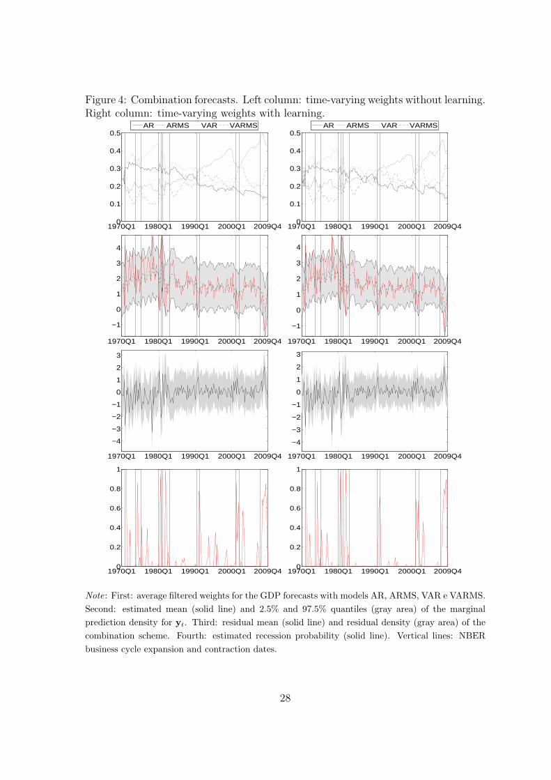
Figure 4: Combination forecasts. Left column: time-varying weights without learning.Right column: time-varying weights with learning.

1970Q1 1980Q1 1990Q1 2000Q1 2009Q40

0.1

0.2

0.3

0.4

0.5

AR ARMS VAR VARMS

1970Q1 1980Q1 1990Q1 2000Q1 2009Q40

0.1

0.2

0.3

0.4

0.5

AR ARMS VAR VARMS

1970Q1 1980Q1 1990Q1 2000Q1 2009Q4

−1

0

1

2

3

4

1970Q1 1980Q1 1990Q1 2000Q1 2009Q4

−1

0

1

2

3

4

1970Q1 1980Q1 1990Q1 2000Q1 2009Q4

−4

−3

−2

−1

0

1

2

3

1970Q1 1980Q1 1990Q1 2000Q1 2009Q4

−4

−3

−2

−1

0

1

2

3

1970Q1 1980Q1 1990Q1 2000Q1 2009Q40

0.2

0.4

0.6

0.8

1

1970Q1 1980Q1 1990Q1 2000Q1 2009Q40

0.2

0.4

0.6

0.8

1

Note: First: average filtered weights for the GDP forecasts with models AR, ARMS, VAR e VARMS.

Second: estimated mean (solid line) and 2.5% and 97.5% quantiles (gray area) of the marginal

prediction density for yt. Third: residual mean (solid line) and residual density (gray area) of the

combination scheme. Fourth: estimated recession probability (solid line). Vertical lines: NBER

business cycle expansion and contraction dates.

28

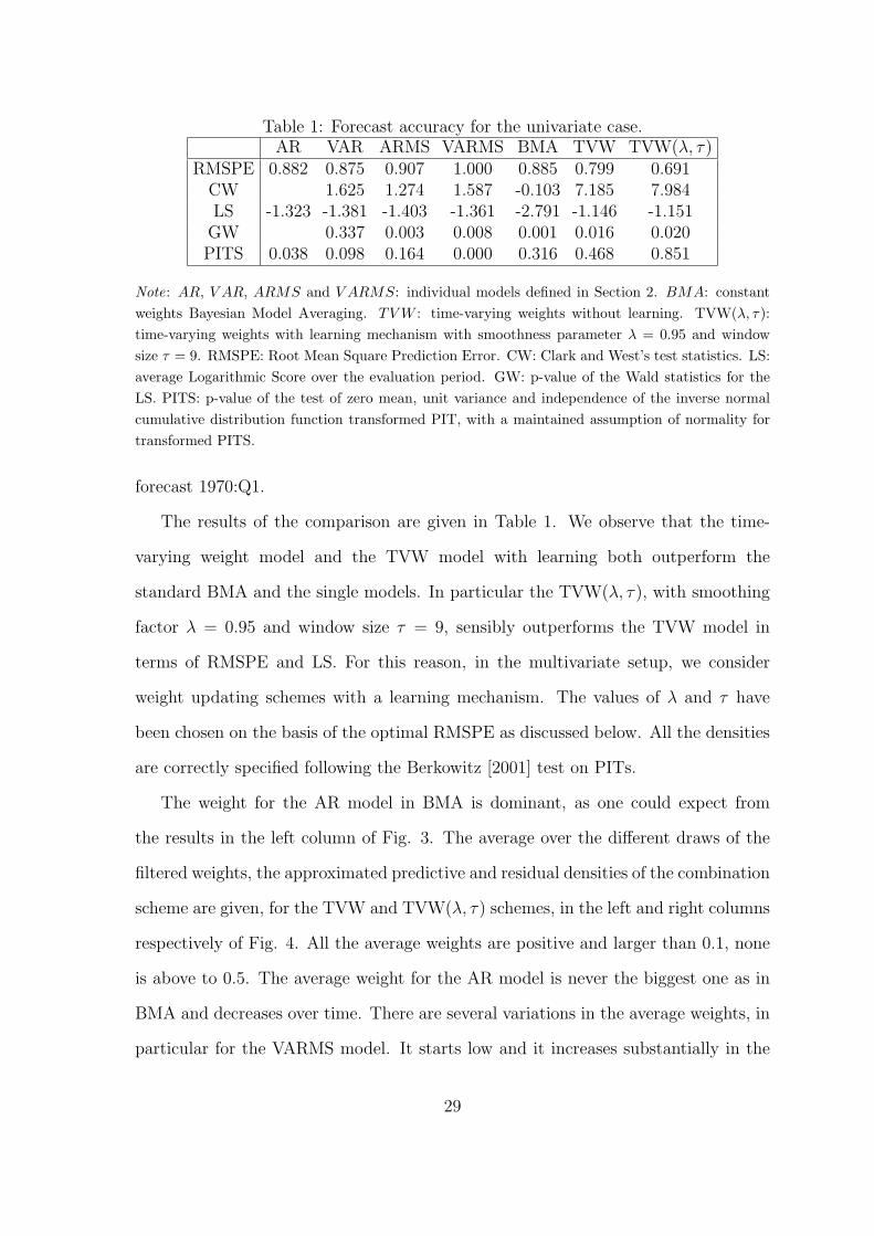
Table 1: Forecast accuracy for the univariate case.AR VAR ARMS VARMS BMA TVW TVW(λ, τ)

RMSPE 0.882 0.875 0.907 1.000 0.885 0.799 0.691CW 1.625 1.274 1.587 -0.103 7.185 7.984LS -1.323 -1.381 -1.403 -1.361 -2.791 -1.146 -1.151GW 0.337 0.003 0.008 0.001 0.016 0.020PITS 0.038 0.098 0.164 0.000 0.316 0.468 0.851

Note: AR, V AR, ARMS and V ARMS: individual models defined in Section 2. BMA: constant

weights Bayesian Model Averaging. TVW : time-varying weights without learning. TVW(λ, τ):

time-varying weights with learning mechanism with smoothness parameter λ = 0.95 and window

size τ = 9. RMSPE: Root Mean Square Prediction Error. CW: Clark and West’s test statistics. LS:

average Logarithmic Score over the evaluation period. GW: p-value of the Wald statistics for the

LS. PITS: p-value of the test of zero mean, unit variance and independence of the inverse normal

cumulative distribution function transformed PIT, with a maintained assumption of normality for

transformed PITS.

forecast 1970:Q1.

The results of the comparison are given in Table 1. We observe that the time-

varying weight model and the TVW model with learning both outperform the

standard BMA and the single models. In particular the TVW(λ, τ), with smoothing

factor λ = 0.95 and window size τ = 9, sensibly outperforms the TVW model in

terms of RMSPE and LS. For this reason, in the multivariate setup, we consider

weight updating schemes with a learning mechanism. The values of λ and τ have

been chosen on the basis of the optimal RMSPE as discussed below. All the densities

are correctly specified following the Berkowitz [2001] test on PITs.

The weight for the AR model in BMA is dominant, as one could expect from

the results in the left column of Fig. 3. The average over the different draws of the

filtered weights, the approximated predictive and residual densities of the combination

scheme are given, for the TVW and TVW(λ, τ) schemes, in the left and right columns

respectively of Fig. 4. All the average weights are positive and larger than 0.1, none

is above to 0.5. The average weight for the AR model is never the biggest one as in

BMA and decreases over time. There are several variations in the average weights, in

particular for the VARMS model. It starts low and it increases substantially in the

29

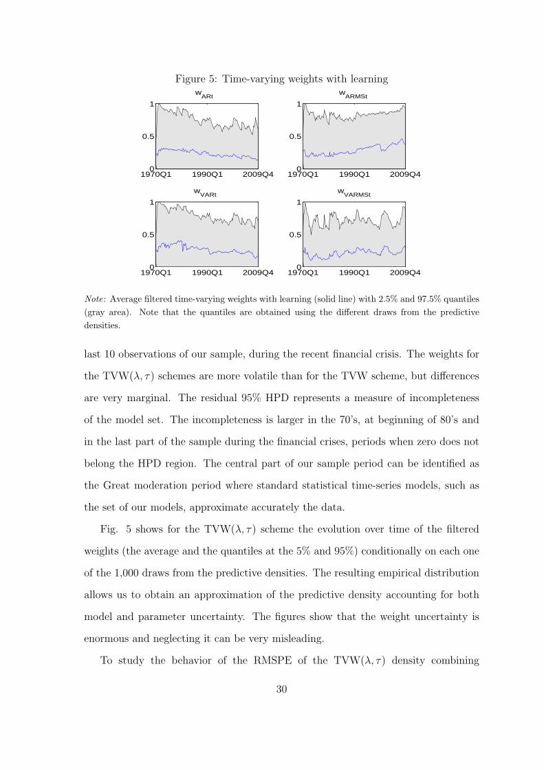
Figure 5: Time-varying weights with learning

1970Q1 1990Q1 2009Q40

0.5

1

wARt

1970Q1 1990Q1 2009Q40

0.5

1

wARMSt

1970Q1 1990Q1 2009Q40

0.5

1

wVARt

1970Q1 1990Q1 2009Q40

0.5

1

wVARMSt

Note: Average filtered time-varying weights with learning (solid line) with 2.5% and 97.5% quantiles

(gray area). Note that the quantiles are obtained using the different draws from the predictive

densities.

last 10 observations of our sample, during the recent financial crisis. The weights for

the TVW(λ, τ) schemes are more volatile than for the TVW scheme, but differences

are very marginal. The residual 95% HPD represents a measure of incompleteness

of the model set. The incompleteness is larger in the 70’s, at beginning of 80’s and

in the last part of the sample during the financial crises, periods when zero does not

belong the HPD region. The central part of our sample period can be identified as

the Great moderation period where standard statistical time-series models, such as

the set of our models, approximate accurately the data.

Fig. 5 shows for the TVW(λ, τ) scheme the evolution over time of the filtered

weights (the average and the quantiles at the 5% and 95%) conditionally on each one

of the 1,000 draws from the predictive densities. The resulting empirical distribution

allows us to obtain an approximation of the predictive density accounting for both

model and parameter uncertainty. The figures show that the weight uncertainty is

enormous and neglecting it can be very misleading.

To study the behavior of the RMSPE of the TVW(λ, τ) density combining

30

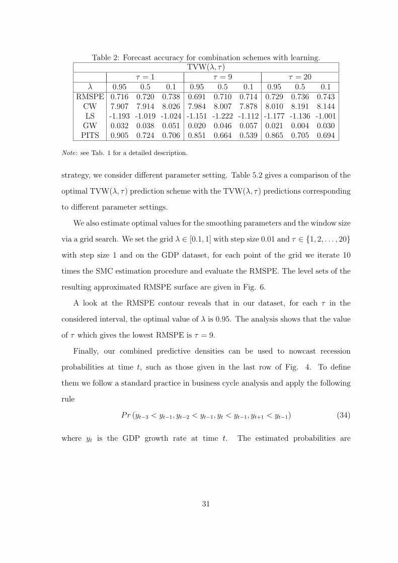
Table 2: Forecast accuracy for combination schemes with learning.TVW(λ, τ)

τ = 1 τ = 9 τ = 20λ 0.95 0.5 0.1 0.95 0.5 0.1 0.95 0.5 0.1

RMSPE 0.716 0.720 0.738 0.691 0.710 0.714 0.729 0.736 0.743CW 7.907 7.914 8.026 7.984 8.007 7.878 8.010 8.191 8.144LS -1.193 -1.019 -1.024 -1.151 -1.222 -1.112 -1.177 -1.136 -1.001GW 0.032 0.038 0.051 0.020 0.046 0.057 0.021 0.004 0.030PITS 0.905 0.724 0.706 0.851 0.664 0.539 0.865 0.705 0.694

Note: see Tab. 1 for a detailed description.

strategy, we consider different parameter setting. Table 5.2 gives a comparison of the

optimal TVW(λ, τ) prediction scheme with the TVW(λ, τ) predictions corresponding

to different parameter settings.

We also estimate optimal values for the smoothing parameters and the window size

via a grid search. We set the grid λ ∈ [0.1, 1] with step size 0.01 and τ ∈ {1, 2, . . . , 20}

with step size 1 and on the GDP dataset, for each point of the grid we iterate 10

times the SMC estimation procedure and evaluate the RMSPE. The level sets of the

resulting approximated RMSPE surface are given in Fig. 6.

A look at the RMSPE contour reveals that in our dataset, for each τ in the

considered interval, the optimal value of λ is 0.95. The analysis shows that the value

of τ which gives the lowest RMSPE is τ = 9.

Finally, our combined predictive densities can be used to nowcast recession

probabilities at time t, such as those given in the last row of Fig. 4. To define

them we follow a standard practice in business cycle analysis and apply the following

rule

Pr (yt−3 < yt−1, yt−2 < yt−1, yt < yt−1, yt+1 < yt−1) (34)

where yt is the GDP growth rate at time t. The estimated probabilities are

31

approximated as follow

1

MN

M∑j=1

N∑i=1

(I(−∞,yt−1)(yt−3)I(−∞,yt−1)(yt−2)I(−∞,yt−1)(yt)I(−∞,yt−1)(y

ijt+1)

)

where yijt+1 is drawn by SMC from p(yt+1|y1:t). The estimated recession probabilities,

in particular those given by the model with learning, fits accurately the US business

cycle and have values higher than 0.5 in each of the recessions identified by the NBER.

Anyway, probabilities seems to lag at beginning of the recessions, which might be due

to the use of GDP as business cycle indicator. Equation (34) could also be extended

to multi-step forecasts to investigate whether timing can improve.

5.3 Multivariate Application to GDP and PCE

We extend the previous combination strategy to the multivariate prediction density of

US GDP and PCE inflation. We still use K = 4 models, and we produce forecasts for

the AR and ARMS for PCE. We use the joint predictive densities for the VAR and the

VARMS. We consider the first and the third combination schemes. BMA averages

models separately for GDP and PCE; our combination method is multivariate by

construction and can combine forecasts for a vector of variables. We apply previous

evaluation statistics and present results individually for each series of interest.

Results in Table 3 are very encouraging. Multivariate combination results in

marginally less accurate point forecasts for GDP, but improve density forecasting in

terms of LS. The TVW(λ, τ) gives the most accurate point and density forecast, and

it is the only approach that gives correct calibrated density at 5% level of significance.

The top plots in Figure 7 show that PCE average weights (or model average

probability) are more volatile than GDP average probability, ARMS has an higher

probability and VARMS a lower probability. VARMS seems the less adequate

32

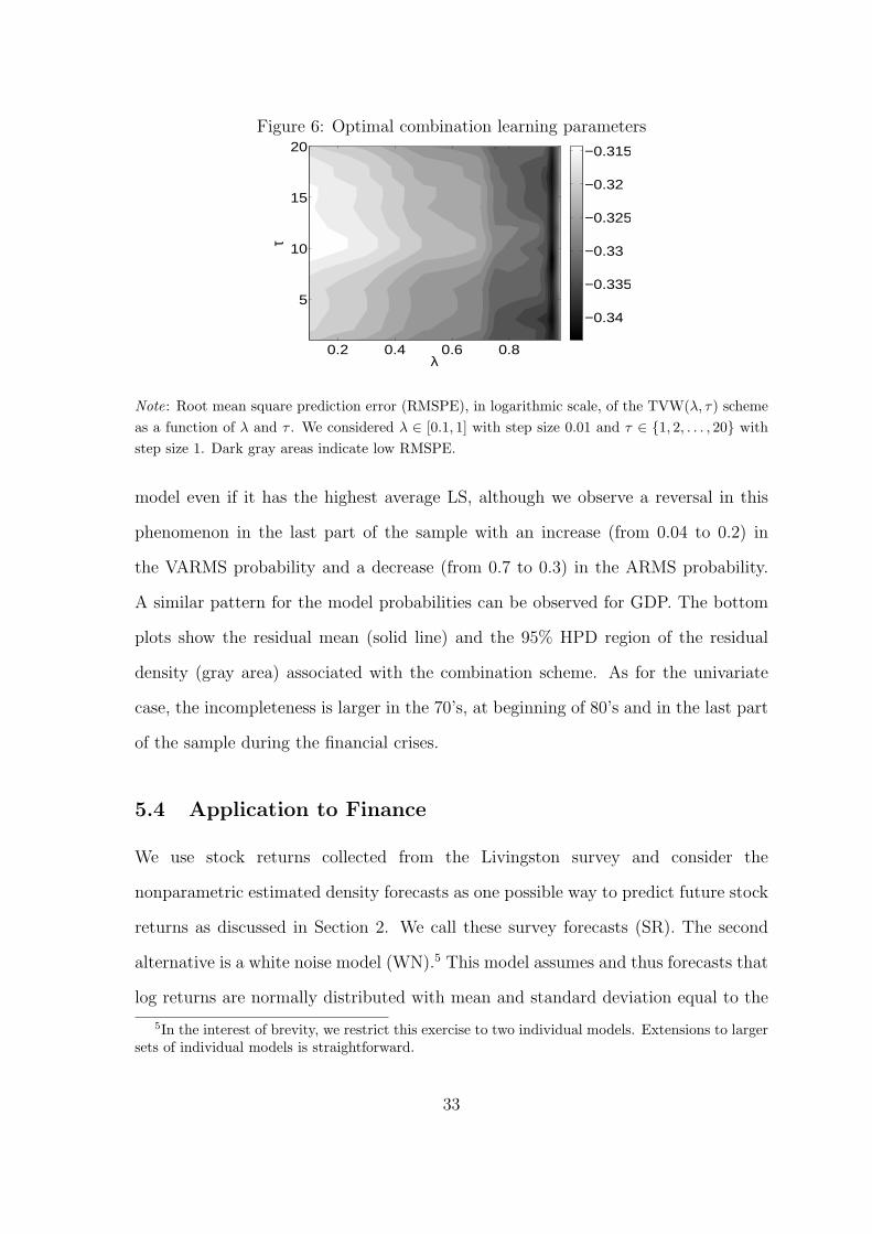
Figure 6: Optimal combination learning parameters

λ

τ

0.2 0.4 0.6 0.8

5

10

15

20

−0.34

−0.335

−0.33

−0.325

−0.32

−0.315

Note: Root mean square prediction error (RMSPE), in logarithmic scale, of the TVW(λ, τ) scheme

as a function of λ and τ . We considered λ ∈ [0.1, 1] with step size 0.01 and τ ∈ {1, 2, . . . , 20} with

step size 1. Dark gray areas indicate low RMSPE.

model even if it has the highest average LS, although we observe a reversal in this

phenomenon in the last part of the sample with an increase (from 0.04 to 0.2) in

the VARMS probability and a decrease (from 0.7 to 0.3) in the ARMS probability.

A similar pattern for the model probabilities can be observed for GDP. The bottom

plots show the residual mean (solid line) and the 95% HPD region of the residual

density (gray area) associated with the combination scheme. As for the univariate

case, the incompleteness is larger in the 70’s, at beginning of 80’s and in the last part

of the sample during the financial crises.

5.4 Application to Finance

We use stock returns collected from the Livingston survey and consider the

nonparametric estimated density forecasts as one possible way to predict future stock

returns as discussed in Section 2. We call these survey forecasts (SR). The second

alternative is a white noise model (WN).5 This model assumes and thus forecasts that

log returns are normally distributed with mean and standard deviation equal to the

5In the interest of brevity, we restrict this exercise to two individual models. Extensions to largersets of individual models is straightforward.

33

Table 3: Results for the multivariate case.GDP

AR VAR ARMS VARMS BMA TVW(λ, τ)RMSPE 0.882 0.875 0.907 1.000 0.885 0.718CW 1.625 1.274 1.587 -0.103 8.554LS -1.323 -1.381 -1.403 -1.361 -2.791 -1.012GW 0.337 0.003 0.008 0.001 0.015PITS 0.038 0.098 0.164 0.000 0.316 0.958

PCEAR VAR ARMS VARMS BMA TVW(λ, τ)

RMSPE 0.385 0.384 0.384 0.612 0.382 0.307CW 1.036 1.902 1.476 1.234 6.715LS -1.538 -1.267 -1.373 -1.090 -1.759 -0.538GW 0.008 0.024 0.007 0.020 0.024PITS 0.001 0.000 0.000 0.000 0.000 0.095

Note: see Tab. 1 for a detailed description.

unconditional (up to time t for forecasting at time t+1) mean and standard deviation.

WN is a standard benchmark to forecast stock returns since it implies a random walk

assumption for prices, which is difficult to beat (see for example Welch and Goyal

[2008]). Finally, we apply our combination scheme from (2) to (4) with time-varying

weights (TVW) with logistic-Gaussian dynamics and learning (see equation (12)).

Following the analysis in Hoogerheide et al. [2010] we evaluate the statistical

accuracy of point forecasts, the survey forecasts and the combination schemes in

terms of the root mean square error (RMSPE), and in terms of the correctly predicted

percentage of sign (Sign Ratio) for the log percent stock index returns. We also

evaluate the statistical accuracy of the density forecasts in terms of the Kullback

Leibler Information Criterion (KLIC) as in the previous section.

Moreover, as an investor is mainly interested in the economic value of a forecasting

model, we develop an active short-term investment exercise, with an investment

horizon of six months. The investor’s portfolio consists of a stock index and risk

free bonds only.6

6The risk free asset is approximated by transforming the monthly federal fund rate in the monththe forecasts are produce in a six month rate. This corresponds to buying a future on the federal

34

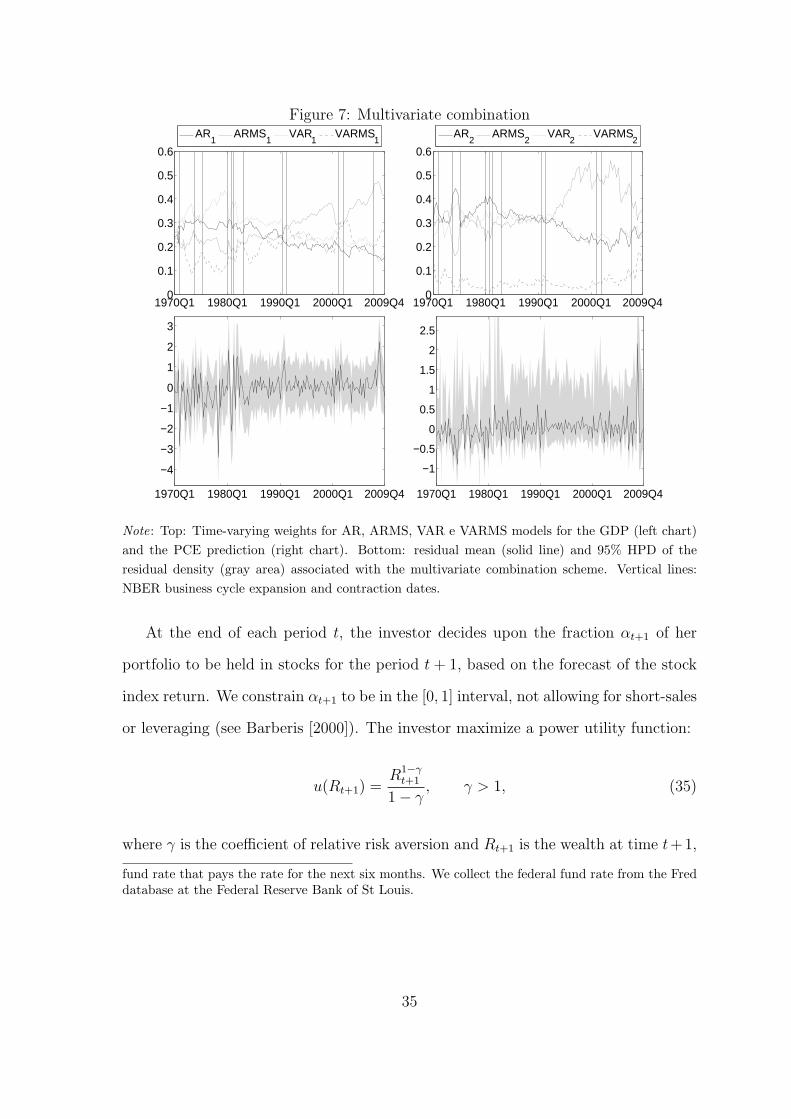
Figure 7: Multivariate combination

1970Q1 1980Q1 1990Q1 2000Q1 2009Q40

0.1

0.2

0.3

0.4

0.5

0.6

AR1

ARMS1

VAR1

VARMS1

1970Q1 1980Q1 1990Q1 2000Q1 2009Q40

0.1

0.2

0.3

0.4

0.5

0.6

AR2

ARMS2

VAR2

VARMS2

1970Q1 1980Q1 1990Q1 2000Q1 2009Q4

−4

−3

−2

−1

0

1

2

3

1970Q1 1980Q1 1990Q1 2000Q1 2009Q4

−1

−0.5

0

0.5

1

1.5

2

2.5

Note: Top: Time-varying weights for AR, ARMS, VAR e VARMS models for the GDP (left chart)

and the PCE prediction (right chart). Bottom: residual mean (solid line) and 95% HPD of the

residual density (gray area) associated with the multivariate combination scheme. Vertical lines:

NBER business cycle expansion and contraction dates.

At the end of each period t, the investor decides upon the fraction αt+1 of her

portfolio to be held in stocks for the period t+ 1, based on the forecast of the stock

index return. We constrain αt+1 to be in the [0, 1] interval, not allowing for short-sales

or leveraging (see Barberis [2000]). The investor maximize a power utility function:

u(Rt+1) =R1−γ

t+1

1− γ, γ > 1, (35)

where γ is the coefficient of relative risk aversion and Rt+1 is the wealth at time t+1,

fund rate that pays the rate for the next six months. We collect the federal fund rate from the Freddatabase at the Federal Reserve Bank of St Louis.

35

which is equal to

Rt+1 = Rt ((1− αt+1) exp(yf,t+1) + αt+1 exp(yf,t+1 + yt+1)), (36)

where Rt denotes initial wealth, yf,t+1 the 1-step ahead risk free rate and yt+1 the

1-step ahead forecast of the stock index return in excess of the risk free made at time

t.

When the initial wealth is set equal to one, i.e. R0 = 1, the investor’s optimization

problem is given by

maxαt+1∈[0,1]

Et

(((1− αt+1) exp(yf,t+1) + αt+1 exp(yf,t+1 + yt+1))

1−γ

1− γ

),

This expectation depends on the predictive density for the excess returns, yt+1.

Following notation in section 4, denoting this density as p(yt+1|y1:t), the investor

solves the following problem:

maxαt+1∈[0,1]

∫u(Rt+1)p(yt+1|y1:t)dyt+1. (37)

We approximate the integral in (37) by generating with the SMC procedure MN

equally weighted independent draws {ygt+1, wgt+1}MN

g=1 from the predictive density

p(yt+1|y1:t), and then use a numerical optimization method to find:

maxαt+1∈[0,1]

1

MN

MN∑g=1

(((1− αt+1) exp(yf,t+1) + αt+1 exp(yf,t+1 + ygt+1))

1−γ

1− γ

)(38)

We consider an investor who can choose between different forecast densities of the

(excess) stock return yt+1 to solve the optimal allocation problem described above.

We include three cases in the empirical analysis below and assume the investor uses

alternatively the density from the WN individual model, the empirical density from

the Livingston Survey (SR) or finally a density combination (DC) of the WN and SR

36

densities. We apply here the DC scheme used in the previous section.

We evaluate the different investment strategies by computing the ex post

annualized mean portfolio return, the annualized standard deviation, the annualized

Sharpe ratio and the total utility. Utility levels are computed by substituting the

realized return of the portfolios at time t+ 1 into (35). Total utility is then obtained

as the sum of u(Rt+1) across all t∗ = (t − t + 1) investment periods t = t, . . . , t,

where the first investment decision is made at the end of period t. We compare the

wealth provided at time t+ 1 by two resulting portfolios by determining the value of

multiplication factor of wealth ∆ which equates their average utilities. For example,

suppose we compare two strategies A and B.

t∑t=t

u(RA,t+1) =t∑

t=t

u(RB,t+1/ exp(r)). (39)

where u(RA,t+1) and u(RB,t+1) are the wealth provided at time T + 1 by the two

resulting portfolios A and B, respectively. Following West et al. [1993], we interpret

∆ as the maximum performance fee the investor would be willing to pay to switch

from strategy A to strategy B.7 We infer the added value of strategies based on

individual models and the combination scheme by computing ∆ with respect to three

static benchmark strategies: holding stocks only (rs), holding a portfolio consisting

of 50% stocks and 50% bonds (rm), and holding bonds only (rb).

Finally, transaction costs play a non-trivial role since the portfolio weights in the

active investment strategies change every month, and the portfolio must be rebalanced

accordingly. Rebalancing the portfolio at the start of month t + 1 means that the

weight invested in stocks is changed from αt to αt+1. We assume that transaction

costs amount to a fixed percentage c on each traded dollar. As we assume that the

7See, for example, Fleming et al. [2001] for an application with stock returns.

37

initial wealth R0 equals to 1, transaction costs at time t+ 1 are equal to

ct+1 = 2c|αt+1 − αt| (40)

where the multiplication by 2 follows from the fact that the investor rebalances her

investments in both stocks and bonds. The net excess portfolio return is then given

by yt+1 − ct+1. We apply a scenario with transaction costs of c = 0.1%.

Panel A in Table 4 reports statical accuracy forecasting results. The survey

forecasts produce the most accurate point forecasts: its RMSPE is the lowest. The

survey is also the most precise in terms of sign ratio. This seems to confirm evidence

that survey forecasts contain timing information. Evidence is, however, different

in terms of density forecasts: the highest log score is for our combination scheme.

Figure 8 plots density forecasts given by the three approaches. The density forecasts

of the survey are too narrow and therefore highly penalized when missing substantial

drops in stock returns as at the beginning of recession periods. The problem might be

caused by the lack of reliable answers during those periods. However, this assumption

cannot be easily investigated. The score for the WN is marginally lower than for our

model combination. However the interval given by the WN is often too large and

indeed the realization never exceeds the 2.5% and 97.5% percentiles.

Figure 9 shows the combination weights with learning for the individual forecasts.

The weights seem to converge to a {0, 1} optimal solution, where the survey has all

the weight towards the end of the period even if the uncertainty is still substantial.

Changing regulations, increased sophistication of instruments, technological advances

and recent global recessions have increased the value added of survey forecasts,

although forecast uncertainty must be modeled carefully as survey forecasts often

seem too confident. As our distributional state-space representation of the predictive

density assumes that the model space is possible incomplete, it appears to infer

properly forecast uncertainties.

38

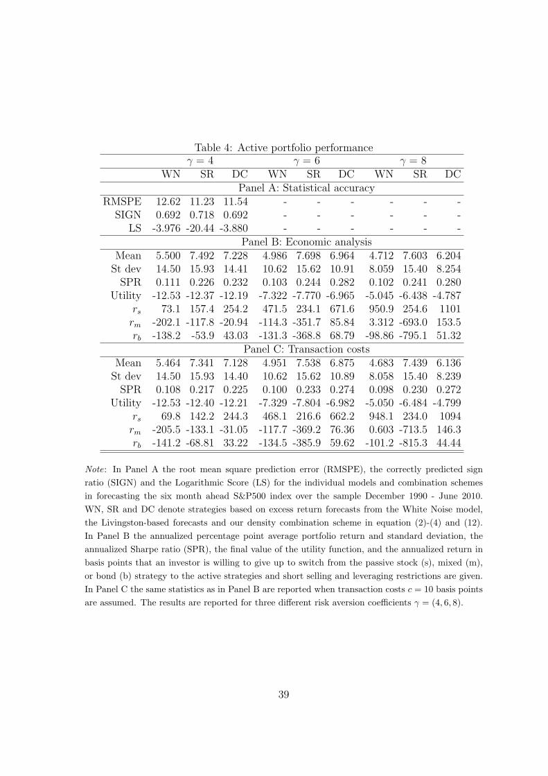
Table 4: Active portfolio performanceγ = 4 γ = 6 γ = 8

WN SR DC WN SR DC WN SR DCPanel A: Statistical accuracy

RMSPE 12.62 11.23 11.54 - - - - - -SIGN 0.692 0.718 0.692 - - - - - -

LS -3.976 -20.44 -3.880 - - - - - -Panel B: Economic analysis

Mean 5.500 7.492 7.228 4.986 7.698 6.964 4.712 7.603 6.204St dev 14.50 15.93 14.41 10.62 15.62 10.91 8.059 15.40 8.254SPR 0.111 0.226 0.232 0.103 0.244 0.282 0.102 0.241 0.280

Utility -12.53 -12.37 -12.19 -7.322 -7.770 -6.965 -5.045 -6.438 -4.787rs 73.1 157.4 254.2 471.5 234.1 671.6 950.9 254.6 1101rm -202.1 -117.8 -20.94 -114.3 -351.7 85.84 3.312 -693.0 153.5rb -138.2 -53.9 43.03 -131.3 -368.8 68.79 -98.86 -795.1 51.32

Panel C: Transaction costsMean 5.464 7.341 7.128 4.951 7.538 6.875 4.683 7.439 6.136St dev 14.50 15.93 14.40 10.62 15.62 10.89 8.058 15.40 8.239SPR 0.108 0.217 0.225 0.100 0.233 0.274 0.098 0.230 0.272

Utility -12.53 -12.40 -12.21 -7.329 -7.804 -6.982 -5.050 -6.484 -4.799rs 69.8 142.2 244.3 468.1 216.6 662.2 948.1 234.0 1094rm -205.5 -133.1 -31.05 -117.7 -369.2 76.36 0.603 -713.5 146.3rb -141.2 -68.81 33.22 -134.5 -385.9 59.62 -101.2 -815.3 44.44

Note: In Panel A the root mean square prediction error (RMSPE), the correctly predicted sign

ratio (SIGN) and the Logarithmic Score (LS) for the individual models and combination schemes

in forecasting the six month ahead S&P500 index over the sample December 1990 - June 2010.

WN, SR and DC denote strategies based on excess return forecasts from the White Noise model,

the Livingston-based forecasts and our density combination scheme in equation (2)-(4) and (12).

In Panel B the annualized percentage point average portfolio return and standard deviation, the

annualized Sharpe ratio (SPR), the final value of the utility function, and the annualized return in

basis points that an investor is willing to give up to switch from the passive stock (s), mixed (m),

or bond (b) strategy to the active strategies and short selling and leveraging restrictions are given.

In Panel C the same statistics as in Panel B are reported when transaction costs c = 10 basis points

are assumed. The results are reported for three different risk aversion coefficients γ = (4, 6, 8).

39

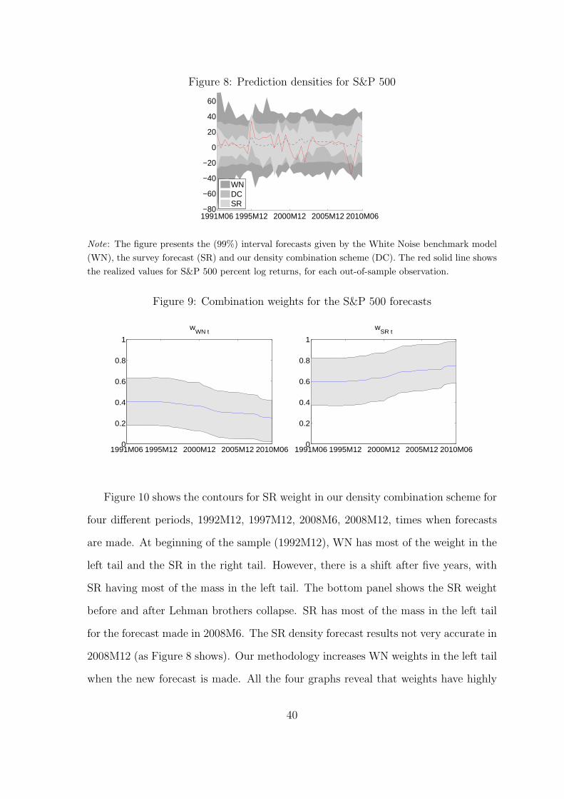
Figure 8: Prediction densities for S&P 500

1991M06 1995M12 2000M12 2005M12 2010M06−80

−60

−40

−20

0

20

40

60

WNDCSR

Note: The figure presents the (99%) interval forecasts given by the White Noise benchmark model

(WN), the survey forecast (SR) and our density combination scheme (DC). The red solid line shows

the realized values for S&P 500 percent log returns, for each out-of-sample observation.

Figure 9: Combination weights for the S&P 500 forecasts

1991M06 1995M12 2000M12 2005M12 2010M060

0.2

0.4

0.6

0.8

1

wWN t

1991M06 1995M12 2000M12 2005M12 2010M060

0.2

0.4

0.6

0.8

1

wSR t

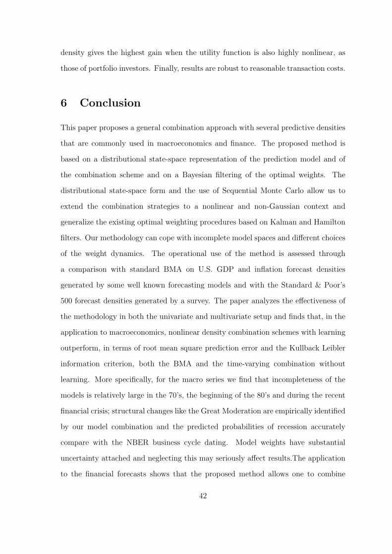
Figure 10 shows the contours for SR weight in our density combination scheme for

four different periods, 1992M12, 1997M12, 2008M6, 2008M12, times when forecasts

are made. At beginning of the sample (1992M12), WN has most of the weight in the

left tail and the SR in the right tail. However, there is a shift after five years, with

SR having most of the mass in the left tail. The bottom panel shows the SR weight

before and after Lehman brothers collapse. SR has most of the mass in the left tail

for the forecast made in 2008M6. The SR density forecast results not very accurate in

2008M12 (as Figure 8 shows). Our methodology increases WN weights in the left tail

when the new forecast is made. All the four graphs reveal that weights have highly

40

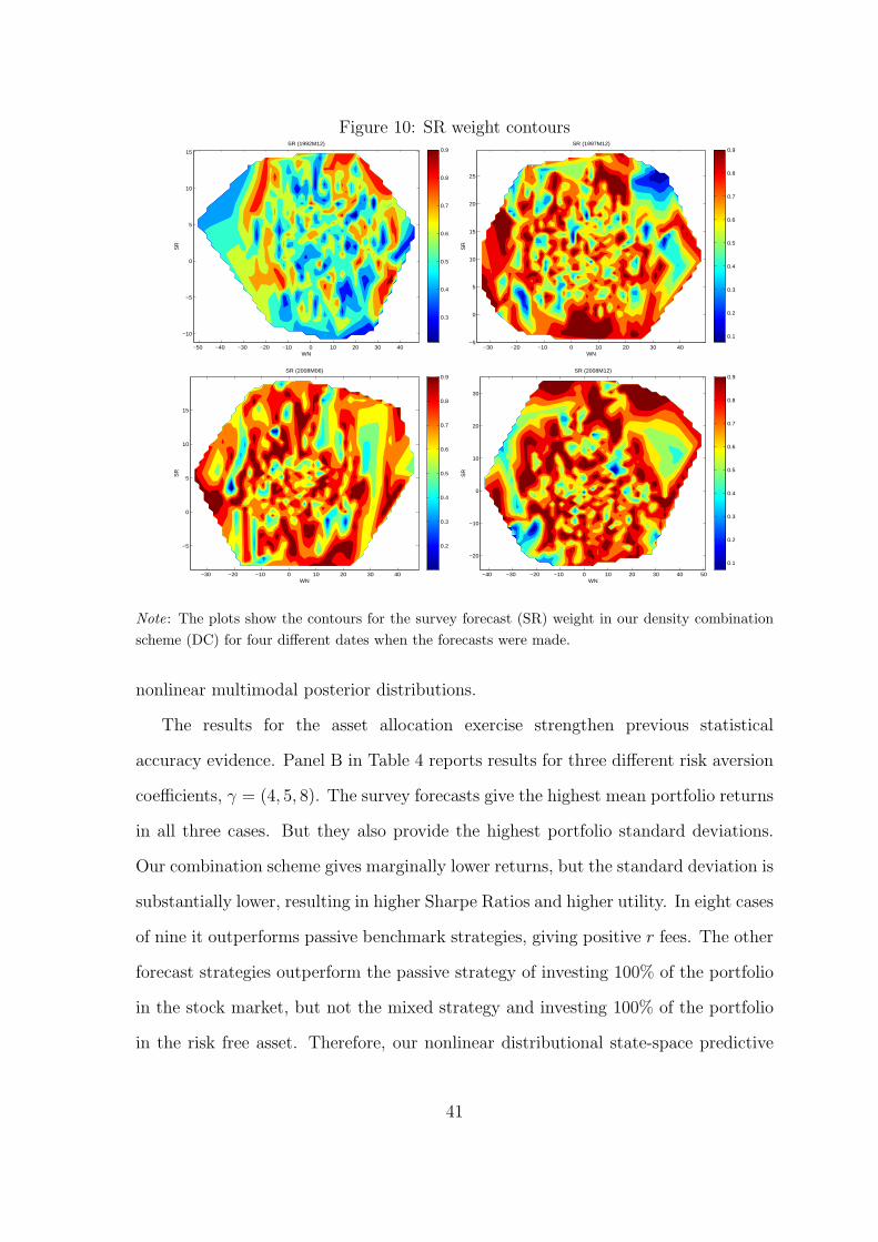
Figure 10: SR weight contours

WN

SR

SR (1992M12)

−50 −40 −30 −20 −10 0 10 20 30 40

−10

−5

0

5

10

15

0.3

0.4

0.5

0.6

0.7

0.8

0.9

WN

SR

SR (1997M12)

−30 −20 −10 0 10 20 30 40−5

0

5

10

15

20

25

0.1

0.2

0.3

0.4

0.5

0.6

0.7

0.8

0.9

WN

SR

SR (2008M06)

−30 −20 −10 0 10 20 30 40

−5

0

5

10

15

0.2

0.3

0.4

0.5

0.6

0.7

0.8

0.9

WN

SR

SR (2008M12)

−40 −30 −20 −10 0 10 20 30 40 50

−20

−10

0

10

20

30

0.1

0.2

0.3

0.4

0.5

0.6

0.7

0.8

0.9

Note: The plots show the contours for the survey forecast (SR) weight in our density combination

scheme (DC) for four different dates when the forecasts were made.

nonlinear multimodal posterior distributions.

The results for the asset allocation exercise strengthen previous statistical

accuracy evidence. Panel B in Table 4 reports results for three different risk aversion

coefficients, γ = (4, 5, 8). The survey forecasts give the highest mean portfolio returns

in all three cases. But they also provide the highest portfolio standard deviations.

Our combination scheme gives marginally lower returns, but the standard deviation is

substantially lower, resulting in higher Sharpe Ratios and higher utility. In eight cases

of nine it outperforms passive benchmark strategies, giving positive r fees. The other

forecast strategies outperform the passive strategy of investing 100% of the portfolio

in the stock market, but not the mixed strategy and investing 100% of the portfolio

in the risk free asset. Therefore, our nonlinear distributional state-space predictive

41

density gives the highest gain when the utility function is also highly nonlinear, as

those of portfolio investors. Finally, results are robust to reasonable transaction costs.

6 Conclusion

This paper proposes a general combination approach with several predictive densities

that are commonly used in macroeconomics and finance. The proposed method is

based on a distributional state-space representation of the prediction model and of

the combination scheme and on a Bayesian filtering of the optimal weights. The

distributional state-space form and the use of Sequential Monte Carlo allow us to

extend the combination strategies to a nonlinear and non-Gaussian context and

generalize the existing optimal weighting procedures based on Kalman and Hamilton

filters. Our methodology can cope with incomplete model spaces and different choices

of the weight dynamics. The operational use of the method is assessed through

a comparison with standard BMA on U.S. GDP and inflation forecast densities

generated by some well known forecasting models and with the Standard & Poor’s

500 forecast densities generated by a survey. The paper analyzes the effectiveness of

the methodology in both the univariate and multivariate setup and finds that, in the

application to macroeconomics, nonlinear density combination schemes with learning

outperform, in terms of root mean square prediction error and the Kullback Leibler

information criterion, both the BMA and the time-varying combination without

learning. More specifically, for the macro series we find that incompleteness of the

models is relatively large in the 70’s, the beginning of the 80’s and during the recent

financial crisis; structural changes like the Great Moderation are empirically identified

by our model combination and the predicted probabilities of recession accurately

compare with the NBER business cycle dating. Model weights have substantial

uncertainty attached and neglecting this may seriously affect results.The application

to the financial forecasts shows that the proposed method allows one to combine

42

forecast densities of different nature, model-based and survey-based, and that it gives

the best prediction performance in terms of utility-based measures. More specifically,

with respect to the returns of the S&P 500 series we find that an investment strategy

using a combination of predictions from professional forecasters and from a white

noise model puts more weight on the white noise model in the beginning of the

90’s and switches to giving more weight to the left tail of the professional forecasts

during the start of the financial crisis around 2008. Information on the complete

predictive distribution and not just basic moments turns out to be important in all

cases investigated.

Appendix A - Combination schemes

Combining Prediction Density

As an alternative to the Gaussian distribution used in section 2.3, heavy-tailed

distributions could be used to account for extreme values which are not captured

by the pool of predictive densities.

Example 1 - (Student-t combination scheme)

In this scheme the conditional density of the observable is

p(yt|Wt, yt) ∝(1 +

1

ν(yt −Wtyt)

′ Σ−1 (yt −Wtyt)

)− ν+L2

(41)

where Σ is the precision matrix and ν > 2 is the degrees-of-freedom parameter. The

scheme could be extended to asymmetric Student-t as in Li et al. [2010].�

Example 2 - (Mixture of experts)

Similarly to Jordan and Jacobs [1994] and Huerta et al. [2003], the density of the

43

observable is

p(yt|yt) =K∑k=1

p (Wk,t|y1:t−1, y1:t−1) p (yk,t) (42)

where p (Wt|y1:t−1, y1:t−1) is the mixture weight associated to model k, which might

be specified similarly to forms in section 3.

Such expression does not allow for the the assumption that all models are false and

in the limit one of the weight will tend to one as discussed in Amisano and Geweke

[2010].�

Weights

We present two alternatives to the continuous weights we have discussed in 3.

Example 3 - (Dirichlet Weights)

The weight model based on the multivariate logistic transform does not lead to an

easy analytical evaluation of the dependence structure between the weights. An

alternative specification of the weight dynamics makes use of the Dirichlet distribution

DK (α1, . . . , αK) in order to define a Dirichlet autoregressive model.

xlt ∼ DKL

(ηl1,tϕ, . . . , η

lKL−1,tϕ, η

lKL,tϕ

)(43)

where ϕ > 0 is the precision parameter and ηlt = g(wl

t−1) with wlt ⊥ εls, ∀ s, t. Due

to the property of the Dirichlet random variable, the multivariate transform of the

latent process is the identity function and it possible to set wlt = xl

t.

An advantage of using the Dirichlet model is that it is naturally defined on the

standard K-dimensional simplex and that the conditional mean and variance and the

covariance can be easily calculated. See for example the seminal paper of Grunwald

et al. [1993] for a nonlinear time series model for data defined on the standard simplex.

The main drawback in the use of this weighting distribution is that, conditional

44

on the past, the correlation between the weights is negative. Moreover it is not easy

to model dependence between the observable and the weights. A possible way would

be to introduce dependence through a common latent factor. We leave these issues

as topics for future research.

�

Moreover, we consider weights with discontinuous dynamics. In fact, in many

applied contexts the discontinuity (e.g. due to structural breaks) in the data

generating process (DGP) calls for a sudden change of the current combination of

the prediction densities.

Example 4 - (Markov-switching Weighting Schemes) We suggest the use of Markov-

switching processes to account for the discontinuous dynamics of the weights. In

fact, in many applied contexts the discontinuity (e.g. due to structural breaks) in the

data generating process calls for a sudden variation of the current combination of the

predictive densities.

We focus on Gaussian combination schemes with the learning mechanism

presented in the section 2.3. The weight specification strategies, presented in the

following, can, however, be easily extended to more general models to account for a

more complex dependence structure between the weights of different components for

the various predictors yk,t.

Consider the following Markov-switching scheme.

p(yt|Wt,Σt, yt) ∝ exp

{−1

2(yt −Wtyt)

′ Σ−1t (yt −Wtyt)

}(44)

Σt =R−1∑r=0

DrI{r}(st) (45)

st ∼ P (st = i|st−1 = j) = pij, ∀i, j ∈ {0, . . . , R− 1} (46)

45

where Dr are positive define matrices. The l-th row of Wt is wlt = g(xl

t) and is a

function of the latent factors xlt and ξt = (ξ1,t, . . . , ξL,t)

′ with the following dynamics

p(xt|xt−1,µt, y1:t−1)∝ exp

{−1

2(∆xt − µt +∆et)

′ Λ−1 (∆xt − µt +∆et)

}(47)

µt = (µ1,t, . . . , µKL2,t)′} (48)

µl,t =

Q−1∑r=0

dl,rI{r}(ξl,t) (49)

ξl,t ∼ P (ξl,t = i|ξl,t−1 = j) = pij, (50)

∀i, j ∈ {0, . . . , Q− 1}, with l = 1, . . . , KL2. We assume ξl,t ⊥ su ∀t, u and ξl,t ⊥ ξj,u

∀l = j and ∀s, t.

It is possible to reduce the number of parameters to be estimated by considering

the following Markov-switching weighting structure

p(yt|Wt, st, yt)∝ exp

{−1

2

(yt −

K∑k=1

wk,t ⊙ yk,t

)′

Σ−1st

(yt −

K∑k=1

wk,t ⊙ yk,t

)}(51)

Σst = Σψ(st) + (1− ψ(st))IL (52)

st ∼ P (st = i|st−1 = j) = pij, ∀i, j ∈ {0, 1} (53)

with wk,t = (w1k,t, . . . , w

Lk,t)

′ and ψ(st) : {0, 1} 7→ [0, 1]. We let ψ(0) = 1 and

ψ(0) > ψ(1) as identifiability constraint.

The dynamics of wlt = (wl

1,t, . . . , wlK,t)

′ = g(xlt) is driven by the latent factors

p(xlt|xl

t,µlt, y1:t−1) ∝ exp

{−1

2

(∆xl

t − µlt +∆elt

)′Λ−1

(∆xl

t − µlt +∆elt

)}(54)

µlt = µ0 + (µ1 − µ0)ξl,t (55)

ξl,t ∼ P (ξl,t = i|ξl,t−1 = j) = pij, ∀i, j ∈ {0, 1} (56)

with l = 1, . . . , L. We assume µk,0 < µk,1 for identifiability purposes and ξl,t ⊥ su

∀t, u and ξl,t ⊥ ξj,u ∀l = j and ∀s, t.�

46

Appendix B - Sequential Monte Carlo

As an example of the filtering procedure applied in our analysis, we give in the

following the pseudo-code of a simple sequential Monte Carlo procedure adapted to

the basic TVW model. See Creal [2009] for a recent survey on the field of sequential

Monte Carlo methods and their applications to economics. Let xt be the vector of

transformed weights and assume, to simplify the exposition, that the parameters are

known. Then at time t with t = 1, . . . , t, the SMC algorithm performs the following

steps:

− Given {Ξjt}Mj=1, with Ξj

t = {xi,jt , ω

i,jt }Ni=1 and for j = 1, . . . ,M

• Generate yjt+1 from p(yj

t+1|y1:t)

• For i = 1, . . . , N

1. Generate xi,jt+1 from NK(x

i,jt ,Λ)

2. Generate yi,jt+1 from p(yt+1|xi,j

t+1, y1t+1, . . . , y

Mt+1)

3. Update the weights

ωi,jt+1 ∝ ωi,j

t exp

{−0.5

(yt+1 −

K∑k=1

wi,jk,ty

jk,t

)′

Σ−1

(yt+1 −

K∑k=1

wi,jk,ty

jk,t

)}

where wi,jk,t = exp(xi,jk,t)/

∑Kk=1 exp{x

i,jk,t}

• Evaluate the Effective Sample Size (ESSjt )

• Normalize the weights ωi,jt+1 = ωi,j

t+1/∑N

i=1 ωi,jt+1 for i = 1, . . . , N

• If ESSjt ≤ κ then resample from Ξj

t

47

References

G. Amisano and J. Geweke. Optimal prediction pools. Journal of Econometrics, 164

(2):130–141, 2010.

G. Amisano and R. Giacomini. Comparing density forecasts via weighted likelihood

ratio tests. Journal of Business & Economic Statistics, 25(2):177–190, 2007.

A. Ang, G. Bekaert, and M. Wei. Do macro variables, asset markets, or surveys

forecast inflation better? Journal of Monetary Economics, 54(4):1163–1212, 2007.

N. Barberis. Investing for the Long Run When Returns are Predictable. Journal of

Finance, 55:225–264, 2000.

G. A. Barnard. New methods of quality control. Journal of the Royal Statistical

Society, Series A, 126:255–259, 1963.

J. M. Bates and C. W. J. Granger. Combination of Forecasts. Operational Research

Quarterly, 20:451–468, 1969.

J. Berkowitz. Testing Density Forecasts, with Applications to Risk Management.

Journal of Business & Economic Statistics, 19(4):465–74, 2001.

M. Billio and R. Casarin. Identifying Business Cycle Turning Points with Sequential

Monte Carlo: An Online and Real-Time Application to the Euro Area. Journal of

Forecasting, 29:145–167, 2010.

G. Boero, J. Smith, and K. F. Wallis. Uncertainty and disagreement in economic

prediction: the bank of england survey of external forecasters. Economic Journal,

118:1107–1127, 2008.

M. Caporin and J. Pres. Modelling and forecasting wind speed intensity for weather

risk management. Computational Statistics and Data Analysis, forthcoming, 2010.

48

T. Clark and K. West. Approximately Normal Tests for Equal Predictive Accuracy

in Nested Models. Journal of Econometrics, 138(1):291–311, 2007.

D. Creal. A survey of sequential monte carlo methods for economics and finance.

Econometric Reviews, Forthcoming, 2009.

P. Del Moral. Feynman-Kac Formulae. Springer Verlag, New York, 2004.

F. X. Diebold and P. Pauly. Structural change and the combination of forecasts.

Journal of Forecasting, 6:21–40, 1987.

F. X. Diebold, T. Gunther, and A. S. Tay. Evaluating Density Forecasts with

Applications to Finance and Management. International Economic Review, 39:

863–883, 1998.

A. Doucet, J. G. Freitas, and J. Gordon. Sequential Monte Carlo Methods in Practice.

Springer Verlag, New York, 2001.

E. F. Fama and M. R. Gibbons. A comparison of inflation forecasts. Journal of

Monetary Economics, 13(3):327–348, 1984.

J. Fleming, C. Kirby, and B. Ostdiek. The Economic Value of Volatility Timing.

Journal of Finance, 56:329–352, 2001.

J. Geweke. Complete and Incomplete Econometric Models. Princeton: Priceton

University Press, 2010.

J. Geweke and G. Amisano. Comparing and evaluating Bayesian predictive

distributions of asset returns. International Journal of Forecasting, 26(2):216–230,

2010.

J. Geweke and C. Whiteman. Bayesian forecasting. In G. Elliot, C.W.J. Granger, and

A.G. Timmermann, editors, Handbook of Economic Forecasting. North-Holland,

2006.

49

R. Giacomini and H. White. Tests of conditional predictive ability. Econometrica, 74

(6):1545–1578, 2006.

C. W. J. Granger. Invited review combining forecasts - twenty years later. Journal

of Forecasting, 8:167–173, 2006.

C. W. J. Granger and R. Ramanathan. Improved Methods of Combining Forecasts.

Journal of Forecasting, 3:197–204, 1984.

J. Groen, R. Paap, and F. Ravazzolo. Real-Time Inflation Forecasting in a Changing

World. Technical Report, 2009.

G. K. Grunwald, A. E. Raftery, and P. Guttorp. Time series of continuous proportions.

Journal of the Royal Statistical Society, Series B, 55:103–116, 1993.

M. Guidolin and A. Timmermann. Forecasts of US Short-term Interest Rates: A

Flexible Forecast Combination Approach. Journal of Econometrics, 150:297–311,

2009.

B. Hansen. Least squares model averaging. Econometrica, 75:1175–1189, 2007.

B. Hansen. Least squares forecast averaging. Journal of Econometrics, 146:342–350,

2008.

J. Harrison and M. West. Bayesian Forecasting and Dynamic Models, 2nd Ed.

Springer Verlag, New York, 1997.

J. A. Hoeting, D. Madigan, A. E. Raftery, and C. T. Volinsky. Bayesian Model

Averaging: A Tutorial. Statistical Science, 14:382–417, 1999.

L. Hoogerheide, R. Kleijn, R. Ravazzolo, H. K. van Dijk, and M. Verbeek. Forecast

Accuracy and Economic Gains from Bayesian Model Averaging using Time Varying

Weights. Journal of Forecasting, 29(1-2):251–269, 2010.

50

G. Huerta, W. Jiang, and M. Tanner. Time series modeling via hierarchical mixtures.

Statistica Sinica, 13:1097–1118, 2003.

M. I. Jordan and R. A. Jacobs. Hierarchical mixtures of experts and the em algorithm.

Neural Computation, 6:181–214, 1994.

A. S. Jore, J. Mitchell, and S. P. Vahey. Combining forecast densities from VARs

with uncertain instabilities. Journal of Applied Econometrics, 25(4):621–634, 2010.

C. Kascha and F. Ravazzolo. Combining Inflation Density Forecasts. Journal of

Forecasting, 29(1-2):231–250, 2010.

Y. Kitamura. Econometric Comparisons of Conditional Models. Discussion paper,,

University of Pennsylvania, 2002.

G. Koop. Bayesian Econometrics. John Wiley and Sons, 2003.

K. Lahiri and X. Sheng. Measuring forecast uncertainty by disagreement: the missing

link. Journal of Applied Econometrics, 128:137–164, 2010.

M. Lanne. Properties of Market-Based and Survey Macroeconomic Forecasts for

Different Data Releases. Economics Bulletin, 29(3):2231–2240, 2009.

F. Legland and N. Oudjane. Stability and uniform approximation of nonlinear filters

using the Hilbert metric and application to particle filters. The Annals of Applied

Probability, 14(1):144–187, 2004.

F. Li, R. Kohn, and M. Villani. Flexible modelling of conditional distributions using

smooth mixtures of asymmetric student t densities. Journal of Statistical Planning

and Inference, 140:3638–3654, 2010.

H. Liang, G. Zou, A.T.K. Wan, and X. Zhang. Optimal weight choice for

frequentist model averaging estimator. Journal of American Statistical Association,

forthcoming, 2011.

51

J. S. Liu and M. West. Combined parameter and state estimation in simulation based

filtering. In A. Doucet, N. de Freitas, and N. Gordon, editors, Sequential Monte

Carlo Methods in Practice. Springer-Verlag, 2001.

Y. P. Mehra. Survey measures of expected inflation : revisiting the issues of predictive

content and rationality. Economic Quarterly, 3:17–36, 2002.

J. Mitchell and S. G. Hall. Evaluating, comparing and combining density forecasts

using the KLIC with an application to the Bank of England and NIESER “fan”

charts of inflation. Oxford Bulletin of Economics and Statistics, 67:995–1033, 2005.

J. Mitchell and K. F. Wallis. Evaluating Density Forecasts: Forecast Combinations,

Model Mixtures, Calibration and Sharpness. Journal of Applied Econometrics,

forthcoming, 2010.

C. Musso, N. Oudjane, and F. Legland. Improving regularised particle filters. In

A. Doucet, N. de Freitas, and N. Gordon, editors, Sequential Monte Carlo Methods

in Practice. Springer-Verlag, 2001.

A. E. Raftery, T. Gneiting, F. Balabdaoui, and M. Polakowski. Using Bayesian Model

Averaging to Calibrate Forecast Ensembles. Monthly Weather Review, 133:1155–

1174, 2005.

H. V. Roberts. Probabilistic prediction. Journal of American Statistical Association,

60:50–62, 1965.

B. W. Silverman. Density estimation for statistics and data analysis. Chapman and

Hall, London, 1986.

J.M. Sloughter, T. Gneiting, and A. E. Raftery. Probabilistic Wind Speed Forecasting

Using Ensembles and Bayesian Model Averaging. Journal of the American

Statistical Association, 105:25–35, 2010.

52

N. Terui and H. K. van Dijk. Combined forecasts from linear and nonlinear time

series models. International Journal of Forecasting, 18:421–438, 2002.

L. B. Thomas. Survey Measures of Expected U.S. Inflation. Journal of Economic

Perspectives, 13(4):125–144, 1999.

A. Timmermann. Forecast combinations. In G. Elliot, C.W.J. Granger, and

A.G. Timmermann, editors, North-Holland, volume 1 of Handbook of Economic

Forecasting, chapter 4, pages 135–196. Elsevier, 2006.

I. Welch and A. Goyal. A Comprehensive Look at the Empirical Performance of

Equity Premium prediction. Review of Financial Studies, 21(4):253–303, 2008.

K. D. West, H. J. Edison, and D. Cho. A utility-based comparison of some models of

exchange rate volatility. Journal of International Economics, 35(1-2):23–45, 1993.

R. L. Winkler. Combining probability distributions from dependent information

sources. Management Science, 27:479–488, 1981.

V. Zarnowitz. Consensus and uncertainty in economic prediction. National Bureau

of Economic Research, 17:492–518, 1992.

53