combining uncertain and paradoxical evidences for dsm hybrid models

arX

iv:m

ath/

0310

135v

2 [

mat

h.D

S] 3

May

200

4

Combining uncertain and paradoxical

evidences for DSm hybrid models

Jean DezertONERA

29 Avenue de la Division Leclerc92320 Chatillon, France.

[email protected]

Florentin SmarandacheDepartment of MathematicsUniversity of New MexicoGallup, NM 87301, U.S.A.

[email protected]

Abstract – This paper presents a general method for combining uncertain and paradoxical source of evidencesfor a wide class of fusion problems. From the foundations of the Dezert-Smarandache Theory (DSmT) we showhow the DSm rule of combination can be adapted to take into account all possible integrity constraints (if any)of the problem under consideration due to the true nature of elements/concepts involved into it. We show howthe Shafer’s model can be considered as a specific DSm hybrid model and be easily handled by our approach anda new efficient rule of combination different from the Dempster’s rule is obtained. Several simple examples arealso provided to show the efficiency and the generality of the approach proposed in this work.

Keywords: DSmT, uncertain and paradoxical reasoning, hybrid-model, data fusion.

MSC 2000: 68T37, 94A15, 94A17, 68T40.

1 IntroductionA new theory of plausible and paradoxical reasoning (DSmT) has been developed by the authors in the

last two years in order to resolve problems that did not work in Dempster-Shafer and other fusion theories.According to each model/problem of fusion occurring, we develop here a DSm hybrid rule which combines twoor more masses of independent sources of information and takes care of restraints, i.e. of sets which mightbecome empty at time tl or new sets/elements that might arise in the frame of discernment at time tl+1. DSmhybrid rule is applied in a real time when the hyper-power set DΘ changes (i.e. the set of all propositions builtfrom elements of frame Θ with ∪ and ∩ operators - see[9] for details), either increasing or decreasing its fo-cal elements, or when even Θ decreases or increases influencing the DΘ as well, thus the dynamicity of our DSmT.

The paper introduces the reader to the independence of sources of evidences, which needs to be deeper studiedin the future, then defines the models and the DSm hybrid rule, which is different from other rules of combinationsuch as Dempster’s, Yager’s, Smets’, Dubois-Prade’s and gives seven numerical examples of applying the DSmhybrid rule in various models and several examples of dynamicity of DSmT, then the Bayesian DSm hybridmodels mixture.

2 On the independence of the sources of evidencesThe notion on independence of sources of evidences plays a major role in the development of efficient

data fusion algorithms but is very difficult to formally establish when manipulating uncertain and paradoxicalinformation. Some attempts to define the independence of uncertain sources of evidences have been proposedby P. Smets and al. in the Dempster-Shafer Theory (DST) and Transferable Belief Model in [20, 21, 22]and by other authors in possibility theory [2, 3, 11, 14, 18]. In the following we consider that n sourcesof evidences are independent if the internal mechanism by which each source provides its own basic beliefassignment doesn’t depend on the mechanisms of other sources (i.e. there is no internal relationship betweenall mechanisms) or if the sources don’t share (even partially) same knowledge/experience to establish their own

1

http://lanl.arXiv.org/abs/math/0310135v2

2

basic belief assignment. This definition doesn’t exclude the possibility for independent sources to provide thesame (numerical) basic belief assignments. The fusion of dependent uncertain and paradoxical sources is muchmore complicated because, one has first to identify precisely the piece of redundant information between sourcesin order to remove it before applying fusion rules. The problem of combination of dependent sources is underinvestigation.

3 DSm rule of combination for free-DSm models

3.1 Definition of the free-DSm model Mf(Θ)

Let consider a finite frame Θ = {θ1, . . . θn} of the fusion problem under consideration. We abandon theShafer’s model by assuming here that the fuzzy/vague/relative nature of elements θi i = 1, . . . , n of Θ can benon-exclusive. We assume also that no refinement of Θ into a new finer exclusive frame of discernment Θref

is possible. This is the free-DSm model Mf (Θ) which can be viewed as the opposite (if we don’t introducenon-existential constraints - see next section) of Shafer’s model, denoted M0(Θ) where all θi are forced to beexclusive and therefore fully discernable.

3.2 Example of a free-DSm model

Let consider the frame of the problem Θ = {θ1, θ2, θ3}. The free Dedekind’s lattice DΘ = {α0, . . . , α18} overΘ owns the following 19 elements [7, 9]

Elements of DΘ for Mf (Θ)

α0 , ∅α1 , θ1 ∩ θ2 ∩ θ3 6= ∅α2 , θ1 ∩ θ2 6= ∅ α3 , θ1 ∩ θ3 6= ∅ α4 , θ2 ∩ θ3 6= ∅α5 , (θ1 ∪ θ2) ∩ θ3 6= ∅ α6 , (θ1 ∪ θ3) ∩ θ2 6= ∅ α7 , (θ2 ∪ θ3) ∩ θ1 6= ∅α8 , {(θ1 ∩ θ2) ∪ θ3} ∩ (θ1 ∪ θ2) 6= ∅α9 , θ1 6= ∅ α10 , θ2 6= ∅ α11 , θ3 6= ∅α12 , (θ1 ∩ θ2) ∪ θ3 6= ∅ α13 , (θ1 ∩ θ3) ∪ θ2 6= ∅ α14 , (θ2 ∩ θ3) ∪ θ1 6= ∅α15 , θ1 ∪ θ2 6= ∅ α16 , θ1 ∪ θ3 6= ∅ α17 , θ2 ∪ θ3 6= ∅α18 , θ1 ∪ θ2 ∪ θ3 6= ∅

The free-DSm model Mf (Θ) assumes that all elements αi, i > 0, are non-empty. This corresponds to thefollowing Venn diagram where in the Smarandache’s codification ”i” denotes the part of the diagram whichbelongs to θi only, ”ij” denotes the part of the diagram which belongs to θi and θj only, ”ijk” denotes thepart of the diagram which belongs to θi and θj and θk only, etc [9]. On such Venn diagram representation ofthe model, we emphasize the fact that all boundaries of intersections must be seen/interpreted as only vagueboundaries just because the nature of elements θi can be, in general, only vague, relative and imprecise.

Figure 1: Venn Diagram for Mf (Θ)

We now recall the classical DSm rule of combination based Mf(Θ) over the free Dedekind’s lattice builtfrom elements of Θ with ∩ and ∪ operators, i.e. the hyper-power set DΘ.

3

3.3 Classical DSm rule for 2 sources for free-DSm models

For two independent uncertain and paradoxical sources of information (experts/bodies of evidence) providinggeneralized basic belief assignment m1(.) and m2(.) over DΘ (or over any subset of DΘ), the classical DSmconjunctive rule of combination mMf (Θ)(.) , [m1 ⊕ m2](.) is given by [7]

∀A 6= ∅ ∈ DΘ, mMf (Θ)(A) , [m1 ⊕ m2](A) =∑

X1,X2∈DΘ

(X1∩X2)=A

m1(X1)m2(X2) (1)

mMf (Θ)(∅) = 0 by definition, unless otherwise specified in special cases when some source assigns a non-zerovalue to it (like in the Smets TBM approach [17]). This classic DSm rule of combination working on free-DSm models is commutative and associative. This rule, dealing with both uncertain and paradoxist/conflictinginformation, requires no normalization process and can always been applied.

3.4 Classical DSm rule for k ≥ 2 sources for free-DSm models

The above formula can be easily generalized for the free-DSm model Mf (Θ) with k ≥ 2 independent sourcesin the following way:

∀A 6= ∅ ∈ DΘ, mMf (Θ)(A) , [m1 ⊕ . . .mk](A) =∑

X1,...,Xk∈DΘ

(X1∩...∩Xk)=A

k∏

i=1

mi(Xi) (2)

mMf (Θ)(∅) = 0 by definition, unless otherwise specified in special cases when some source assigns a non-zerovalue to it. This classic DSm rule of combination is still commutative and associative.

4 Presentation of DSm hybrid models

4.1 Definition

Let Θ be the general frame of the fusion problem under consideration with n elements θ1, θ2, . . ., θn. A DSmhybrid model M(Θ) is defined from the free-DSm model Mf (Θ) by introducing some integrity constraints onsome elements A of DΘ if one knows with certainty the exact nature of the model corresponding to the problemunder consideration. An integrity constraint on A consists in forcing A to be empty (vacuous element), and we

will denote such constraint as AM≡ ∅ which means that A has been forced to ∅ through the model M(Θ). This

can be justified by the knowledge of the true nature of each element θi of Θ. Indeed, in some fusion problems,some elements θi and θj of Θ can be fully discernable because they are truly exclusive while other elementscannot be refined into finer exclusive elements. Moreover, it is also possible that for some reason with some newknowledge on the problem, an element or several elements θi have to be forced to the empty set (specially ifdynamical fusion problems are considered, i.e when Θ varies with space and time). For example, if we considera list of three potential suspects into a police investigation, it can occur that, during the investigation, one ofthe suspect must be stray off the initial frame of the problem if he can prove his gullibility with an ascertainablealibi. The initial basic belief masses provided by sources of information one had on the three suspects, mustthen be modified by taking into account this new knowledge on the model of the problem.

There exists several possible kinds of integrity constraints which can be introduced in any free-DSm modelMf (Θ) actually. The first kind of integrity constraint concerns exclusivity constraints by taking into account

that some conjunctions of elements θi, . . . , θk are truly impossible (i.e. θi ∩ . . . ∩ θk

M≡ ∅). The second kind

of integrity constraint concerns the non-existential constraints by taking into account that some disjunctions

of elements θi, . . . , θk are also truly impossible (i.e. θi ∪ . . . ∪ θk

M≡ ∅). We exclude from our presentation the

completely degenerate case corresponding to the constraint θ1 ∪ . . . ∪ θn

M≡ ∅ (total ignorance) because there is

no way and interest to treat such vacuous problem. In such degenerate case, we can just set m(∅) , 1 which isuseless because the problem remains vacuous and DΘ reduces to ∅. The last kind of possible integrity constraintis a mixture of the two previous ones, like for example (θi∩θj)∪θk or any other hybrid proposition/element of DΘ

involving both ∩ and ∪ operators such that at least one element θk is subset of the constrained proposition. Fromany Mf (Θ), we can thus build several DSm hybrid models depending on the number of integrity constraints

4

one wants to fully characterize the nature of the problem. The introduction of a given integrity constraint

AM≡ ∅ ∈ DΘ implies necessarily the set of inner constraints B

M≡ ∅ for all B ⊂ A. Moreover the introduction of

two integrity constraints, say on A and B in DΘ implies also necessarily the constraint on the emptiness of thedisjunction A ∪ B which belongs also to DΘ (because DΘ is close under ∩ and ∪ operators). This implies theemptiness of all C ∈ DΘ such that C ⊂ (A∪B). Same remark has to be extended for the case of the introductionof n integrity constraints as well. The Shafer’s model is the unique and most constrained DSm hybrid modelincluding all possible exclusivity constraints without non-existential constraint since all θi 6= ∅ ∈ Θ are forcedto be mutually exclusive. The Shafer’s model is denoted M0(Θ) in the sequel. We denote by ∅M the set ofelements of DΘ which have been forced to be empty in the DSm hybrid model M.

4.2 Example 1 : DSm hybrid model with an exclusivity constraint

Let Θ = {θ1, θ2, θ3} be the general frame of the problem under consideration and let consider the following

DSm hybrid model M1(Θ) built by introducing the following exclusivity constraint α1 , θ1 ∩ θ2 ∩ θ3M1≡ ∅.

This exclusivity constraint implies however no other constraint because α1 doesn’t contain other elements ofDΘ but itself. Therefore, one has now the following set of elements for DΘ

Elements of DΘ for M1(Θ)

α0 , ∅

α1 , θ1 ∩ θ2 ∩ θ3M1≡ ∅

α2 , θ1 ∩ θ2 6= ∅ α3 , θ1 ∩ θ3 6= ∅ α4 , θ2 ∩ θ3 6= ∅α5 , (θ1 ∪ θ2) ∩ θ3 6= ∅ α6 , (θ1 ∪ θ3) ∩ θ2 6= ∅ α7 , (θ2 ∪ θ3) ∩ θ1 6= ∅α8 , {(θ1 ∩ θ2) ∪ θ3} ∩ (θ1 ∪ θ2) 6= ∅α9 , θ1 6= ∅ α10 , θ2 6= ∅ α11 , θ3 6= ∅α12 , (θ1 ∩ θ2) ∪ θ3 6= ∅ α13 , (θ1 ∩ θ3) ∪ θ2 6= ∅ α14 , (θ2 ∩ θ3) ∪ θ1 6= ∅α15 , θ1 ∪ θ2 6= ∅ α16 , θ1 ∪ θ3 6= ∅ α17 , θ2 ∪ θ3 6= ∅α18 , θ1 ∪ θ2 ∪ θ3 6= ∅

Hence the initial basic belief mass over DΘ has to be transferred over the new constrained hyper-power setDΘ(M1(Θ)) with the 18 elements defined just above. The mechanism for the transfer of basic belief massesfrom DΘ onto DΘ(M1(Θ)) will be obtained by the DSm hybrid rule of combination presented in the sequel.

4.3 Example 2 : DSm hybrid model with another exclusivity constraint

As second example for DSm hybrid model M2(Θ), let consider Θ = {θ1, θ2, θ3} and the following exclusivity

constraint α2 , θ1 ∩ θ2M2≡ ∅. This constraint implies also α1 , θ1 ∩ θ2 ∩ θ3

M2≡ ∅ since α1 ⊂ α2. Therefore, one

has now the following set of elements for DΘ(M2(Θ))


α0 , ∅

α1 , θ1 ∩ θ2 ∩ θ3M2≡ ∅

α2 , θ1 ∩ θ2M2≡ ∅ α3 , θ1 ∩ θ3 6= ∅ α4 , θ2 ∩ θ3 6= ∅

α5 , (θ1 ∪ θ2) ∩ θ3 6= ∅ α6 , (θ1 ∪ θ3) ∩ θ2M2≡ α4 6= ∅ α7 , (θ2 ∪ θ3) ∩ θ1

M2≡ α3 6= ∅

α8 , {(θ1 ∩ θ2) ∪ θ3} ∩ (θ1 ∪ θ2)M2≡ α5 6= ∅

α9 , θ1 6= ∅ α10 , θ2 6= ∅ α11 , θ3 6= ∅

α12 , (θ1 ∩ θ2) ∪ θ3M2≡ α11 6= ∅ α13 , (θ1 ∩ θ3) ∪ θ2 6= ∅ α14 , (θ2 ∩ θ3) ∪ θ1 6= ∅

α15 , θ1 ∪ θ2 6= ∅ α16 , θ1 ∪ θ3 6= ∅ α17 , θ2 ∪ θ3 6= ∅α18 , θ1 ∪ θ2 ∪ θ3 6= ∅

Note that in this case several non-empty elements of DΘ(M2(Θ)) coincide because of the constraint (α6M2≡ α4,

α7M2≡ α3, α8

M2≡ α5, α12

M2≡ α11). DΘ(M2(Θ)) has now only 13 different elements. Note that the introduction

of both constraints α1 , θ1∩θ2∩θ3M2≡ ∅ and α2 , θ1∩θ2

M2≡ ∅ doesn’t change the construction of DΘ(M2(Θ))

because α1 ⊂ α2.

5

4.4 Example 3 : DSm hybrid model with another exclusivity constraint

As third example for DSm hybrid model M3(Θ), let consider Θ = {θ1, θ2, θ3} and the following exclusivity

constraint α6 , (θ1 ∪ θ3) ∩ θ2M3≡ ∅. This constraint implies now α1 , θ1 ∩ θ2 ∩ θ3

M3≡ ∅ since α1 ⊂ α6, but

also α2 , θ1 ∩ θ2M3≡ ∅ because α2 ⊂ α6 and α4 , θ2 ∩ θ3

M3≡ ∅ because α4 ⊂ α6. Therefore, one has now the

following set of elements for DΘ(M3(Θ))


α0 , ∅

α1 , θ1 ∩ θ2 ∩ θ3M3≡ ∅

α2 , θ1 ∩ θ2M3≡ ∅ α3 , θ1 ∩ θ3 6= ∅ α4 , θ2 ∩ θ3

M3≡ ∅

α5 , (θ1 ∪ θ2) ∩ θ3M3≡ α3 6= ∅ α6 , (θ1 ∪ θ3) ∩ θ2

M3≡ ∅ α7 , (θ2 ∪ θ3) ∩ θ1

M3≡ α3 6= ∅

α8 , {(θ1 ∩ θ2) ∪ θ3} ∩ (θ1 ∪ θ2)M3≡ α5 6= ∅

α9 , θ1 6= ∅ α10 , θ2 6= ∅ α11 , θ3 6= ∅

α12 , (θ1 ∩ θ2) ∪ θ3M3≡ α11 6= ∅ α13 , (θ1 ∩ θ3) ∪ θ2 6= ∅ α14 , (θ2 ∩ θ3) ∪ θ1

M3≡ α9 6= ∅

α15 , θ1 ∪ θ2 6= ∅ α16 , θ1 ∪ θ3 6= ∅ α17 , θ2 ∪ θ3 6= ∅α18 , θ1 ∪ θ2 ∪ θ3 6= ∅

DΘ(M3(Θ)) has now only 10 different elements.

4.5 Example 4 : DSm hybrid model with all exclusivity constraints

As fourth example for DSm hybrid model M4(Θ), let consider Θ = {θ1, θ2, θ3} and the following exclusivity

constraint α8 , {(θ1 ∩ θ2) ∪ θ3} ∩ (θ1 ∪ θ2)M4≡ ∅. This model corresponds actually to the Shafer’s model

M0(Θ) because this constraint includes all possible exclusivity constraints between elements θi, i = 1, 2, 3 sinceα1 , θ1 ∩ θ2 ∩ θ3 ⊂ α8, α2 , θ1 ∩ θ2 ⊂ α8, α3 , θ1 ∩ θ3 ⊂ α8 and α4 , θ2 ∩ θ3 ⊂ α8. Therefore, one has nowthe following set of elements for DΘ(M4(Θ))


α0 , ∅

α1 , θ1 ∩ θ2 ∩ θ3M4≡ ∅

α2 , θ1 ∩ θ2M4≡ ∅ α3 , θ1 ∩ θ3

M4≡ ∅ α4 , θ2 ∩ θ3

M4≡ ∅

α5 , (θ1 ∪ θ2) ∩ θ3M4≡ ∅ α6 , (θ1 ∪ θ3) ∩ θ2

M4≡ ∅ α7 , (θ2 ∪ θ3) ∩ θ1

M4≡ ∅

α8 , {(θ1 ∩ θ2) ∪ θ3} ∩ (θ1 ∪ θ2)M4≡ ∅

α9 , θ1 6= ∅ α10 , θ2 6= ∅ α11 , θ3 6= ∅

α12 , (θ1 ∩ θ2) ∪ θ3M4≡ α11 6= ∅ α13 , (θ1 ∩ θ3) ∪ θ2

M4≡ α10 6= ∅ α14 , (θ2 ∩ θ3) ∪ θ1

M4≡ α9 6= ∅

α15 , θ1 ∪ θ2 6= ∅ α16 , θ1 ∪ θ3 6= ∅ α17 , θ2 ∪ θ3 6= ∅α18 , θ1 ∪ θ2 ∪ θ3 6= ∅

DΘ(M4(Θ)) has now 2|Θ| = 8 different elements and coincides obviously with the classical power set 2Θ.This corresponds to the Shafer’s model and serves as foundation for the Dempster-Shafer Theory.

6

4.6 Example 5 : DSm hybrid model with a non-existential constraint

As fifth example for DSm hybrid model M5(Θ), let consider Θ = {θ1, θ2, θ3} and the following non-existential

constraint α9 , θ1M5≡ ∅. In other words, we remove θ1 from the initial frame Θ = {θ1, θ2, θ3}. This non-

existential constraint implies α1 , θ1 ∩ θ2 ∩ θ3M5≡ ∅, α2 , θ1 ∩ θ2

M5≡ ∅, α3 , θ1 ∩ θ3

M5≡ ∅ and α7 ,

(θ2 ∪ θ3) ∩ θ1M5≡ ∅. Therefore, one has now the following set of elements for DΘ(M5(Θ))


α0 , ∅

α1 , θ1 ∩ θ2 ∩ θ3M5≡ ∅

α2 , θ1 ∩ θ2M5≡ ∅ α3 , θ1 ∩ θ3

M5≡ ∅ α4 , θ2 ∩ θ3 6= ∅

α5 , (θ1 ∪ θ2) ∩ θ3M5≡ α4 6= ∅ α6 , (θ1 ∪ θ3) ∩ θ2

M5≡ α4 6= ∅ α7 , (θ2 ∪ θ3) ∩ θ1

M5≡ ∅

α8 , {(θ1 ∩ θ2) ∪ θ3} ∩ (θ1 ∪ θ2)M5≡ α4 6= ∅

α9 , θ1M5≡ ∅ α10 , θ2 6= ∅ α11 , θ3 6= ∅

α12 , (θ1 ∩ θ2) ∪ θ3M5≡ α11 6= ∅ α13 , (θ1 ∩ θ3) ∪ θ2

M5≡ α10 6= ∅ α14 , (θ2 ∩ θ3) ∪ θ1

M5≡ α4 6= ∅

α15 , θ1 ∪ θ2M5≡ α10 6= ∅ α16 , θ1 ∪ θ3

M5≡ α11 6= ∅ α17 , θ2 ∪ θ3 6= ∅

α18 , θ1 ∪ θ2 ∪ θ3M5≡ α17 6= ∅

DΘ(M5(Θ)) has now 5 different elements and coincides obviously with the hyper-power set DΘ\θ1 .

4.7 Example 6 : DSm hybrid model with two non-existential constraints

As sixth example for DSm hybrid model M6(Θ), let consider Θ = {θ1, θ2, θ3} and the following two non-

existential constraints α9 , θ1M6≡ ∅ and α10 , θ2

M6≡ ∅. Actually, these two constraints are equivalent to choose

only the following constraint α15 , θ1∪θ2M5≡ ∅. In other words, we remove now both θ1 and θ2 from the initial

frame Θ = {θ1, θ2, θ3}. These non-existential constraints implies now α1 , θ1 ∩ θ2 ∩ θ3M6≡ ∅, α2 , θ1 ∩ θ2

M6≡ ∅,

α3 , θ1∩θ3M6≡ ∅, α4 , θ2∩θ3

M6≡ ∅, α5 , (θ1∪θ2)∩θ3

M6≡ ∅, α6 , (θ1∪θ3)∩θ2

M6≡ ∅, α7 , (θ2∪θ3)∩θ1

M6≡ ∅,

α8 , {(θ1 ∩ θ2) ∪ θ3} ∩ (θ1 ∪ θ2)M6≡ ∅, α13 , (θ1 ∩ θ3) ∪ θ2

M6≡ ∅, α14 , (θ2 ∩ θ3) ∪ θ1

M6≡ ∅ . Therefore, one has

now the following set of elements for DΘ(M6(Θ))


α0 , ∅

α1 , θ1 ∩ θ2 ∩ θ3M6≡ ∅

α2 , θ1 ∩ θ2M6≡ ∅ α3 , θ1 ∩ θ3

M6≡ ∅ α4 , θ2 ∩ θ3

M6≡ ∅

α5 , (θ1 ∪ θ2) ∩ θ3M6≡ ∅ α6 , (θ1 ∪ θ3) ∩ θ2

M6≡ ∅ α7 , (θ2 ∪ θ3) ∩ θ1

M6≡ ∅

α8 , {(θ1 ∩ θ2) ∪ θ3} ∩ (θ1 ∪ θ2)M6≡ ∅

α9 , θ1M6≡ ∅ α10 , θ2

M6≡ ∅ α11 , θ3 6= ∅

α12 , (θ1 ∩ θ2) ∪ θ3M6≡ α11 6= ∅ α13 , (θ1 ∩ θ3) ∪ θ2

M6≡ ∅ α14 , (θ2 ∩ θ3) ∪ θ1

M6≡ ∅

α15 , θ1 ∪ θ2M6≡ ∅ α16 , θ1 ∪ θ3

M6≡ α11 6= ∅ α17 , θ2 ∪ θ3

M6≡ α11 6= ∅

α18 , θ1 ∪ θ2 ∪ θ3M6≡ α11 6= ∅

DΘ(M6(Θ)) reduces now to only two different elements ∅ and θ3. DΘ(M6(Θ)) coincides obviously with thehyper-power set DΘ\{θ1,θ2}. Because there exists only one possible non empty element in DΘ(M6(Θ)), suchkind of problem is called a trivial problem. If one now introduces all non-existential constraints in free-DSmmodel, then the initial problem reduces to a vacuous problem also called impossible problem corresponding tom(∅) ≡ 1 (no problem at all since the problem doesn’t not exist now !!!). Such kinds of trivial or vacuousproblems are not considered anymore in the sequel since they present no real interest for engineering data fusionproblems.

7

4.8 Example 7 : DSm hybrid model with a mixed constraint

As seventh example for DSm hybrid model M7(Θ), let consider Θ = {θ1, θ2, θ3} and the following mixed

exclusivity and non-existential constraint α12 , (θ1 ∩ θ2) ∪ θ3M7≡ ∅. This mixed constraint implies α1 ,

θ1 ∩ θ2 ∩ θ3M7≡ ∅, α2 , θ1 ∩ θ2

M7≡ ∅, α3 , θ1 ∩ θ3

M7≡ ∅, α4 , θ2 ∩ θ3

M7≡ ∅, α5 , (θ1 ∪ θ2) ∩ θ3

M7≡ ∅,

α6 , (θ1 ∪ θ3) ∩ θ2M7≡ ∅, α7 , (θ2 ∪ θ3) ∩ θ1

M7≡ ∅, α8 , {(θ1 ∩ θ2) ∪ θ3} ∩ (θ1 ∪ θ2)

M7≡ ∅ and α11 , θ3

M7≡ ∅.

Therefore, one has now the following set of elements for DΘ(M7(Θ))


α0 , ∅

α1 , θ1 ∩ θ2 ∩ θ3M7≡ ∅

α2 , θ1 ∩ θ2M7≡ ∅ α3 , θ1 ∩ θ3

M7≡ ∅ α4 , θ2 ∩ θ3

M7≡ ∅

α5 , (θ1 ∪ θ2) ∩ θ3M7≡ ∅ α6 , (θ1 ∪ θ3) ∩ θ2

M7≡ ∅ α7 , (θ2 ∪ θ3) ∩ θ1

M7≡ ∅

α8 , {(θ1 ∩ θ2) ∪ θ3} ∩ (θ1 ∪ θ2)M7≡ ∅

α9 , θ1 6= ∅ α10 , θ2 6= ∅ α11 , θ3M7≡ ∅

α12 , (θ1 ∩ θ2) ∪ θ3M7≡ ∅ α13 , (θ1 ∩ θ3) ∪ θ2

M7≡ α10 6= ∅ α14 , (θ2 ∩ θ3) ∪ θ1

M7≡ α9 6= ∅

α15 , θ1 ∪ θ2 6= ∅ α16 , θ1 ∪ θ3M7≡ α9 6= ∅ α17 , θ2 ∪ θ3

M7≡ α10 6= ∅

α18 , θ1 ∪ θ2 ∪ θ3M7≡ α15 6= ∅

DΘ(M7(Θ)) reduces now to only four different elements ∅, θ1, θ2, and θ1 ∪ θ2.

5 DSm rule of combination for DSm hybrid modelsWe present in this section a general DSm-hybrid rule of combination able to deal with any DSm hybrid

models. We will show how this new general rule of combination works with all DSm hybrid models presentedin the previous section and we list interesting properties of this new useful and powerful rule of combination.

5.1 Notations

Let Θ = {θ1, . . . θn} be a frame of partial discernment of the constrained fusion problem, and DΘ the freedistributive lattice (hyper-power set) generated by Θ and the empty set ∅ under ∩ and ∪ operators. We needto distinguish between the empty set ∅, which belongs to DΘ, and by ∅ we understand a set which is empty allthe time (we call it absolute emptiness or absolutely empty) independent of time, space and model, and all othersets from DΘ. For example θ1 ∩ θ2 or θ1 ∪ θ2 or only θi itself, 1 ≤ i ≤ n, etc, which could be or become emptyat a certain time (if we consider a fusion dynamicity) or in a particular model M (but could not be empty inother model and/or time) (we call a such element relative emptiness or relatively empty). Well denote by ∅M

the set of relatively empty such elements of DΘ (i.e. which become empty in a particular model M or at aspecific time). ∅M is the set of integrity constraints which depends on the DSm model M under consideration,and the model M depends on the structure of its corresponding fuzzy Venn Diagram (number of elements inΘ, number of non-empty intersections, and time in case of dynamic fusion). Through our convention ∅ /∈ ∅M.Lets note by ∅ , {∅, ∅M} the set of all relatively and absolutely empty elements.

For any A ∈ DΘ, let φ(A) be the characteristic emptiness function of the set A, i.e. φ(A) = 1 if A /∈ ∅ andφ(A) = 0 otherwise. This function helps in assigning the value zero to all relatively or absolutely empty elementsof DΘ through the choice of DSm hybrid model M. Let’s define the total ignorance on Θ = {θ1, θ2, . . . , θn} asIt , θ1∪θ2∪. . .∪θn and the set of relative ignorances as Ir , {θi1∪. . .∪θik

, where i1, ..., ik ∈ {1, 2, ..., n} and 2 ≤k ≤ n − 1}, then the set of all kind of ignorances as I = It ∪ Ir. For any element A in DΘ, one considers u(A)as the union of all singletons θi that compose A. For example, if A is a singleton then u(A) = A; if A = θ1 ∩ θ2

or A = θ1 ∪ θ2 then u(A) = θ1 ∪ θ2; if A = (θ1 ∩ θ2) ∪ θ3 then u(A) = θ1 ∪ θ2 ∪ θ3. ; by convention u(∅) , ∅.The second summation of the DSm hybrid rule (see eq. (3) and (5) and denoted S2 in the sequel) transfers themass of ∅ [if any; sometimes, in rare cases, m(∅) > 0 (for example in Ph. Smets’ work); we want to catch thisparticular case as well] to the total ignorance It = θ1 ∪ θ2 ∪ . . . ∪ θn. The other part of the mass of relativelyempty elements, θi and θj together for example, i 6= j, goes to the partial ignorance/uncertainty m(θi ∪ θj). S2

8

multiplies, naturally following the DSm classic network architecture, only the elements of columns of absolutelyand relatively empty sets, and then S2 transfers the mass m1(X1)m2(X2) . . . mk(Xk) either to the elementA ∈ Dθ in the case when A = u(X1) ∪ u(X2) ∪ . . . ∪ u(Xk) is not empty, or if u(X1) ∪ u(X2) ∪ . . . ∪ u(Xk)is empty then the mass m1(X1)m2(X2)mk(Xk) is transferred to the total ignorance. We include all possibledegenerate problems/models in this new DSmT hybrid framework, but the vacuous DSm-hybrid model M∅

defined by the constraint It = θ1 ∪ θ2 ∪ . . . ∪ θn

M∅≡ ∅ which is meaningless and useless.

We provide here the issue for programming the calculation of u(X) from the binary representation of anyproposition X ∈ DΘ expressed in the Dezert-Smarandache’s order [9, 8]. Let’s consider the Smarandache’s cod-ification of elements θ1, . . . , θn. One defines the anti-absorbing relationship as follows: element i anti-absorbselement ij (with i < j), and let’s use the notation i << ij, and also j << ij; similarly ij << ijk (withi < j < k), also jk << ijk and ik << ijk. This relationship is transitive, therefore i << ij and ij << ijkinvolve i << ijk; one can also write i << ij << ijk as a chain; similarly one gets j << ijk and k << ijk.The anti-absorbing relationship can be generalized for parts with any number of digits, i.e. when one uses theSmarandache codification for the corresponding Venn diagram on Θ = {θ1, θ2, . . . , θn}, with n ≥ 1. Betweenelements ij and ik, or between ij and jk there is no anti-absorbing relationship, therefore the anti-absorbingrelationship makes a partial order on the parts of the Venn diagram for the free DSm model. If a propositionX is formed by a part only, say i1i2 . . . ir, in the Smarandache codification, then u(X) = θi1 ∪ θi2 ∪ . . . ∪ θir

.If X is formed by two or more parts, the first step is to eliminate all anti-absorbed parts, ie. if A << B thenu(A, B) = u(A); generally speaking, a part B is anti-absorbed by part A if all digits of A belong to B; for ananti-absorbing chain A1 << A2 << ... << As one takes A1 only and the others are eliminated; afterwards,when X is anti-absorbingly irreducible, u(X) will be the unions of all singletons whose indices occur in theremaining parts of X - if one digit occurs many times it is taken only once.

See some examples for the case n = 3: 12 << 123, i.e. 12 anti-absorbs 123. Between 12 and 23 there is noanti-absorbing relationship.

• If X = 123 then u(X) = θ1 ∪ θ2 ∪ θ3.

• If X = {23, 123}, then 23 << 123, thus u({23, 123}) = u(23), because 123 has been eliminated, henceu(X) = u(23) = θ2 ∪ θ3.

• If X = {13, 123}, then 13 << 123, thus u({13, 123}) = u(13) = θ1 ∪ θ3.

• If X = {13, 23, 123}, then 13 << 123, thus u({13, 23, 123}) = u({13, 23}) = θ1 ∪ θ2 ∪ θ3 (one takes astheta indices each digit in the {13, 23}) - if one digit is repeated it is taken only once; between 13 and 23there is no relation of anti-absorbing.

• If X = {3, 13, 23, 123}, then u(X) = u({3, 13, 23}) because 23 << 123, then u({3, 13, 23}) = u({3, 13})because 3 << 23, then u({3, 13}) = u(3) = θ3 because 3 << 13.

• If X = {1, 12, 13, 23, 123}, then one has the anti-absorbing chain: 1 << 12 << 123, thus u(X) =u({1, 13, 23}) = u({1, 23}) because 1 << 13, and finally u(X) = θ1 ∪ θ2 ∪ θ3.

• If X = {1, 2, 12, 13, 23, 123}, then 1 << 12 << 123 and 2 << 23 thus u(X) = u({1, 2, 13}) = u({1, 2})because 1 << 13, and finally u(X) = θ1 ∪ θ2.

• If X = {2, 12, 3, 13, 23, 123}, then 2 << 23 << 123 and 3 << 13 thus u(X) = u({2, 12, 3}), but 2 << 12hence u(X) = u({2, 3}) = θ2 ∪ θ3.

9

5.2 The DSm hybrid rule of combination for 2 sources

To eliminate the degenerate vacuous fusion problem from the presentation, we assume from now on that thegiven DSm hybrid model M under consideration is always different from the vacuous model M∅ (i.e. It 6= ∅).The DSm hybrid rule of combination, associated to a given DSm hybrid model M 6= M∅ , for two sources isdefined for all A ∈ DΘ as:

mM(Θ)(A) , φ(A)[

∑

X1,X2∈DΘ

(X1∩X2)=A

m1(X1)m2(X2)

+∑

X1,X2∈∅

[(u(X1)∪u(X2))=A]∨[(u(X1)∪u(X2)∈∅)∧(A=It)]

m1(X1)m2(X2)

+∑

X1,X2∈DΘ

(X1∪X2)=A

X1∩X2∈∅

m1(X1)m2(X2)]

(3)

The first sum entering in the previous formula corresponds to mass mMf (Θ)(A) obtained by the classic DSm

rule of combination (1) based on the free-DSm model Mf (i.e. on the free lattice DΘ), i.e.

mMf (Θ)(A) ,∑

X1,X2∈DΘ

X1∩X2=A

m1(X1)m2(X2) (4)

The second sum entering in the formula of the DSm-hybrid rule of combination (3) represents the mass of allrelatively and absolutely empty sets which is transferred to the total or relative ignorances.

The third sum entering in the formula of the DSm-hybrid rule of combination (3) transfers the sum of relativelyempty sets to the non-empty sets in the same way as it was calculated following the DSm classic rule.

5.3 The DSm hybrid rule of combination for k ≥ 2 sources

The previous formula of DSm hybrid rule of combination can be generalized in the following way for allA ∈ DΘ :

mM(Θ)(A) , φ(A)[

∑

X1,X2,...,Xk∈DΘ

(X1∩X2∩...∩Xk)=A

k∏

i=1

mi(Xi)

+∑

X1,X2,...,Xk∈∅

[(u(X1)∪u(X2)∪...∪u(Xk))=A]∨[(u(X1)∪u(X2)∪...∪u(Xk)∈∅)∧(A=It)]

k∏

i=1

mi(Xi)

+∑

X1,X2,...,Xk∈DΘ

(X1∪X2∪...∪Xk)=A

X1∩X2∩...∩Xk∈∅

k∏

i=1

mi(Xi)]

(5)

The first sum entering in the previous formula corresponds to mass mMf (Θ)(A) obtained by the classic DSm

rule of combination (2) for k sources of information based on the free-DSm model Mf (i.e. on the free latticeDΘ), i.e.

mMf (Θ)(A) ,∑

X1,X2,...,Xk∈DΘ

(X1∩X2∩...∩Xk)=A

k∏

i=1

mi(Xi) (6)

10

5.4 Remark on the DSm hybrid rule of combination

From (5) and (6), the previous general formula can be rewritten as

mM(Θ)(A) , φ(A)[

S1(A) + S2(A) + S3(A)]

(7)

where

S1(A) ≡ mMf (Θ)(A) ,∑

X1,X2,...,Xk∈DΘ

(X1∩X2∩...∩Xk)=A

k∏

i=1

mi(Xi) (8)

S2(A) ,∑

X1,X2,...,Xk∈∅

[(u(X1)∪u(X2)∪...∪u(Xk))=A]∨[(u(X1)∪u(X2)∪...∪u(Xk)∈∅)∧(A=It)]

k∏

i=1

mi(Xi) (9)

S3(A) ,∑

X1,X2,...,Xk∈DΘ

(X1∪X2∪...∪Xk)=A

X1∩X2∩...∩Xk∈∅

k∏

i=1

mi(Xi) (10)

and thus, this combination can be viewed actually as a two steps procedure as follows:

• Step 1: Evaluate the combination of the sources over the free lattice DΘ by the classical DSm rule ofcombination to get for all A ∈ DΘ, S1(A) = mMf (Θ)(A) using (6). This step preserves the commutativityand associativity properties of the combination.

• Step 2 : Transfer the masses of the integrity constraints of the DSm hybrid model M according to formula(7). Note that this step is necessary only if one has reliable information about the real constraints involvedin the fusion problem under consideration.

The second step does not preserve the associativity property but this is not a fundamental requirement inmost of fusion systems actually. If one really wants to preserve optimality of the fusion rule, one has first tocombine all sources using classical DSm rule (with any clustering of sources) and the ultimate step will consistto adapt basic belief masses according to the integrity constraints of the model M.

If one first adapts the local basic belief masses m1(.), ...mk(.) to the hybrid-model M and afterwards oneapplies the combination rules, the fusion result becomes only suboptimal because some information is lost dur-ing the transfer of masses of integrity constraints. The same remark holds if the transfer of masses of integrityconstraints is done at some intermediate steps after the fusion of m sources with m < k.

Let’s note also that this formula of transfer is more general (because we include the possibilities to introduceboth exclusivity constraints and non-existential constraints as well) and more precise (because we explicitlyconsider all different relative emptiness of elements into the general transfer formula (7)) than the generictransfer formulas used in the DST framework proposed as alternative rules to the Dempster’s rule of combination[12] and discussed in section 5.9.

11

5.5 Property of the DSm Hybrid Rule

∑

A∈DΘ

mM(Θ)(A) =∑

A∈DΘ

φ(A)[

S1(A) + S2(A) + S3(A)]

= 1 (11)

Proof: Let’s first prove that∑

A∈DΘ m(A) = 1 where all masses m(A) are obtained by the DSm classic rule.Let’s consider each mass mi(.) provided by the ith source of information, for 1 ≤ i ≤ k, as a vector of d = | DΘ |dimension, whose sum of components is equal to one, i.e. mi(D

Θ) = [mi1, mi2, . . . , mid], and∑

j=1,d mij = 1.Thus, for k ≥ 2 sources of information, the mass matrix becomes

M =

m11 m12 . . . m1d

m21 m22 . . . m2d

. . . . . . . . . . . .mk1 mk2 . . . mkd

If one notes the sets in DΘ by A1, A2, ..., Ad (doesn’t matter in what order one lists them) then the column(j) in the matrix represents the masses assigned to Aj by each source of information s1, s2, . . ., sk; for examplesi(Aj) = mij , where 1 ≤ i ≤ k. According to the DSm network architecture [9], all the products in this networkwill have the form m1j1m2j2 . . .mkjk

, i.e. one element only from each matrix row, and no restriction about thenumber of elements from each matrix column, 1 ≤ j1, j2, . . . , jk ≤ d. Each such product will enter in the fusionmass of one set only from DΘ. Hence the sum of all components of the fusion mass is equal to the sum of allthese products, which is equal to

k∏

i=1

d∑

j=1

mij =k

∏

i=1

1 = 1 (12)

The DSm hybrid rule has three sums S1, S2, and S3. Let’s separate the mass matrix M into two disjoint

sub-matrices M∅ formed by the columns of all absolutely and relatively empty sets, and MN formed by thecolumns of all non-empty sets. According to the DSm network architecture (for k ≥ 2 rows):

• S1 is the sum of all products resulted from the multiplications of the columns of MN following the DSmnetwork architecture such that the intersection of their corresponding sets is non-empty, i.e. the sum ofmasses of all non-empty sets before any mass of absolutely or relatively empty sets could be transferredto them;

• S2 is the sum of all products resulted from the multiplications of M∅ following the DSm network archi-tecture, i.e. a partial sum of masses of absolutely and relatively empty sets transferred to the ignorancesin I , It ∪ Ir or to singletons of Θ.

• S3 is the sum of all the products resulted from the multiplications of the columns of MN and M∅ together,following the DSm network architecture, but such that at least a column is from each of them, and alsothe sum of all products of columns of MN such that the intersection of their corresponding sets is empty(what did not enter into the previous sum S1), i.e. the remaining sum of masses of absolutely or relativelyempty sets transferred to the non-empty sets of the DSm hybrid model M.

If one now considers all the terms (each such term is a product of the form m1j1m2j2 . . .mkjk) of these three

sums, we get exactly the same terms as in the DSm network architecture for the DSm classic rule, thus the sumof all terms occurring in S1, S2, and S3 is 1 (see formula (12)) which completes the proof. DSm hybrid rulenaturally derives from the DSm classic rule.

12

Entire masses of relatively and absolutely empty sets in a given DSm hybrid model M are transferred tonon-empty sets according to the above and below formula (7) and thus

∀A ∈ ∅ ⊂ DΘ, mM(Θ)(A) = 0 (13)

The entire mass of a relatively empty set (from DΘ) which has in its expression θj1 , θj2 , . . ., θjr, with 1 ≤ r ≤ n

will generally be distributed among the θj1 , θj2 , . . ., θjror their unions or intersections, and the distribution

follows the way of multiplication from the DSm classic rule, explained by the DSm network architecture [9].Thus, because nothing is lost, nothing is gained, the sum of all mM(Θ)(A) is equal to 1 as just proved previously,and fortunately no normalization constant is needed which could bring a lost of information in the fusion rule.

The three summations S1(.), S3(.) and S3(.) are disjoint because:

• S1(.) multiplies the columns corresponding to non-emptysets only - but such that the intersections of thesets corresponding to these columns are non-empty [following the definition of DSm classic rule];

• S2(.) multiplies the columns corresponding to absolutely and relatively emptysets only;

• S3(.) multiplies:

a) either the columns corresponding to absolutely or relatively emptysets with the columns correspond-ing to non-emptysets such that at least a column corresponds to an absolutely or relatively emptysetand at least a column corresponds to a non-emptyset,

b) or the columns corresponding to non-emptysets - but such that the intersections of the sets corre-sponding to these columns are empty.

The multiplications are following the DSm network architecture, i.e. any product has the above general form:m1j1m2j2 . . . mkjk

, i.e. any product contains as factor one element only from each row of the mass matrix Mand the total number of factors in a product is equal to k. The function φ(A) automatically assigns the valuezero to the mass of any empty set, and allows the calculation of masses of all non-emptysets.

5.6 On the programming of the DSm hybrid rule

We briefly give here an issue for a fast programming of DSm rule of combination. Let’s consider Θ ={θ1, θ2, . . . , θn}, the sources B1, B2,. . ., Bk, and p = min{n, k}. One needs to check only the focal sets, i.e. sets(i.e. propositions) whose masses assigned to them by these sources are not all zero. Thus, if M is the massmatrix, and we consider a set Aj in DΘ, then the column (j) corresponding to Aj , i.e. (m1j m2j . . . mkj)transposed has not to be identical to the null-vector of k-dimension (0 0 . . . 0) transposed. Let DΘ(step1) beformed by all focal sets at the beginning (after sources B1, B2,. . ., Bk have assigned massed to the sets in DΘ).Applying the DSm classic rule, besides the sets in DΘ(step1) one adds r-intersections of sets in DΘ(step1), thus:

DΘ(step2) = DΘ(step1) ∨ {Ai1 ∧ Ai2 ∧ . . . ∧ Air}

where Ai1 , Ai2 , . . . , Airbelong to DΘ(step1) and 2 ≤ r ≤ p.

Applying the DSm hybrid rule, due to its S2 and S3 summations, besides the sets in DΘ(step2) one addsr-unions of sets and the total ignorance in DΘ(step2), thus:

DΘ(step3) = DΘ(step2) ∨ It ∨ {Ai1 ∨ Ai2 ∨ . . . ∨ Air}

where Ai1 , Ai2 , . . . , Airbelong to DΘ(step2) and 2 ≤ r ≤ p.

This means that instead of computing the masses of all sets in DΘ, one needs to first compute the massesof all focal sets (step 1), second the masses of their r-intersections (step 2), and third the masses of r-unions ofall previous sets and the mass of total ignorance (step 3).

13

5.7 Application of the DSm Hybrid rule on previous examples

We present in this section some numerical results of the DSm hybrid rule of combination for 2 independentsources of information. We examine the seven previous examples in order to help the reader to check by himselfor herself the validity of our new general formula. Due to space limitation, we will not go in details on allthe derivations steps, we will just present main intermediary results (i.e. the value of the three summations)involved into the general formula (3). The results have been first obtained by hands and then be validated byMatLab programming. We denote

S1(A) ≡ mMf (Θ)(A) ,∑

X1,X2∈DΘ

X1∩X2=A

m1(X1)m2(X2)

S2(A) ,∑

X1,X2∈∅

[u(X1)∪u(X2)=A]∨[(u(X1)∪u(X2)∈∅)∧(A=It)]

m1(X1)m2(X2)

S3(A) ,∑

X1,X2∈DΘ

X1∪X2=A

X1∩X2∈∅

m1(X1)m2(X2)

Now let consider Θ = {θ1, θ2, θ3} and the two following independent bodies of evidence B1 and B2 with thegeneralized basic belief assignments1 m1(.) and m2(.) given in the following table2. The right column of thetable indicates the result of the fusion obtained by the classical DSm rule of combination.

Element A of DΘ m1(A) m2(A) mMf (Θ)(A)

∅ 0 0 0θ1 ∩ θ2 ∩ θ3 0 0 0.16θ2 ∩ θ3 0 0.20 0.19θ1 ∩ θ3 0.10 0 0.12(θ1 ∪ θ2) ∩ θ3 0 0 0.01θ3 0.30 0.10 0.10θ1 ∩ θ2 0.10 0.20 0.22(θ1 ∪ θ3) ∩ θ2 0 0 0.05(θ2 ∪ θ3) ∩ θ1 0 0 0{(θ1 ∩ θ2) ∪ θ3} ∩ (θ1 ∪ θ2) 0 0 0(θ1 ∩ θ2) ∪ θ3 0 0 0θ2 0.20 0.10 0.03(θ1 ∩ θ3) ∪ θ2 0 0 0θ2 ∪ θ3 0 0 0θ1 0.10 0.20 0.08(θ2 ∩ θ3) ∪ θ1 0 0 0.02θ1 ∪ θ3 0.10 0.20 0.02θ1 ∪ θ2 0.10 0 0θ1 ∪ θ2 ∪ θ3 0 0 0

The following subsections present the numerical results obtained by the DSm hybrid rule on the seven previousexamples. The tables show all the values of φ(A), S1(A), S2(A) and S3(A) to help the reader to check by himselfor herself the validity of these results. It is important to note that the values of S1(A), S2(A) and S3(A) whenφ(A) = 0 do not need to be computed in practice but are provided here only for a checking purpose.

1A general numerical example with m1(A) > 0 and m2(A) > 0 for all A 6= ∅ ∈ DΘ will be briefly presented in next section.2The order of elements of DΘ corresponds here to the order obtained from the generation of isotone Boolean functions - see [9]

for details.

14

5.7.1 Application of the DSm Hybrid rule on example 1

Here is the numerical result corresponding to example 1 with the hybrid-model M1 (i.e with the exclusivity

constraint θ1 ∩ θ2 ∩ θ3M1≡ ∅). The right column of the table provides the result obtained using the DSm hybrid

rule, ie. ∀A ∈ DΘ,mM1(Θ)(A) = φ(A)

[

S1(A) + S2(A) + S3(A)]

Element A of DΘ φ(A) S1(A) S2(A) S3(A) mM1(Θ)(A)∅ 0 0 0 0 0

θ1 ∩ θ2 ∩ θ3M1≡ ∅ 0 0.16 0 0 0

θ2 ∩ θ3 1 0.19 0 0 0.19θ1 ∩ θ3 1 0.12 0 0 0.12(θ1 ∪ θ2) ∩ θ3 1 0.01 0 0.02 0.03θ3 1 0.10 0 0 0.10θ1 ∩ θ2 1 0.22 0 0 0.22(θ1 ∪ θ3) ∩ θ2 1 0.05 0 0.02 0.07(θ2 ∪ θ3) ∩ θ1 1 0 0 0.02 0.02{(θ1 ∩ θ2) ∪ θ3} ∩ (θ1 ∪ θ2) 1 0 0 0 0(θ1 ∩ θ2) ∪ θ3 1 0 0 0.07 0.07θ2 1 0.03 0 0 0.03(θ1 ∩ θ3) ∪ θ2 1 0 0 0.01 0.01θ2 ∪ θ3 1 0 0 0 0θ1 1 0.08 0 0 0.08(θ2 ∩ θ3) ∪ θ1 1 0.02 0 0.02 0.04θ1 ∪ θ3 1 0.02 0 0 0.02θ1 ∪ θ2 1 0 0 0 0θ1 ∪ θ2 ∪ θ3 1 0 0 0 0

DM1 =

0 0 0 0 0 00 0 0 0 0 10 0 0 0 1 00 0 0 0 1 10 0 0 1 1 10 0 1 0 0 00 0 1 0 0 10 0 1 0 1 00 0 1 0 1 10 0 1 1 1 10 1 1 0 0 10 1 1 0 1 10 1 1 1 1 11 0 1 0 1 01 0 1 0 1 11 0 1 1 1 11 1 1 0 1 11 1 1 1 1 1

From the previous table of this first numerical example, we see in column corresponding to S3(A) how theinitial combined mass mMf (Θ)(θ1 ∩ θ2 ∩ θ3) ≡ S1(θ1 ∩ θ2 ∩ θ3) = 0.16 is transferred (due to the constraintof M1) only onto the elements (θ1 ∪ θ2) ∩ θ3, (θ1 ∪ θ3) ∩ θ2, (θ2 ∪ θ3) ∩ θ1, (θ1 ∩ θ2) ∪ θ3, (θ1 ∩ θ3) ∪ θ2, and(θ2 ∩ θ3) ∪ θ1 of DΘ. We can easily check that the sum of the elements of the column for S3(A) is equal tomMf (Θ)(θ1 ∩ θ2 ∩ θ3) = 0.16 as required. Thus after introducing the constraint, the initial hyper-power set DΘ

reduces to 18 elements as follows

DΘM1

= {∅, θ2 ∩ θ3, θ1 ∩ θ3, (θ1 ∪ θ2) ∩ θ3, θ3, θ1 ∩ θ2, (θ1 ∪ θ3) ∩ θ2, (θ2 ∪ θ3) ∩ θ1, {(θ1 ∩ θ2) ∪ θ3} ∩ (θ1 ∪ θ2),

(θ1 ∩ θ2) ∪ θ3, θ2, (θ1 ∩ θ3) ∪ θ2, θ2 ∪ θ3, θ1, (θ2 ∩ θ3) ∪ θ1, θ1 ∪ θ3, θ1 ∪ θ2, θ1 ∪ θ2 ∪ θ3}

As detailed in [9], the elements of DΘM1

can be described and encoded by the matrix product DM1 · uM1 withDM1 given above and the basis vector uM1 defined as uM1 = [< 1 >< 2 >< 12 >< 3 >< 13 >< 23 >]′. Actu-ally uM1 is directly obtained from uMf

3 by removing its component < 123 > corresponding to the constraintintroduced by the model M1.

In general, the encoding matrix DM for a given DSm hybrid model M is obtained from DMf by removingall its columns corresponding to the constraints of the chosen model M and all the rows corresponding toredundant/equivalent propositions. In this particular example with model M1, we will just have to remove thelast column of DMf to get DM1 and no row is removed from DMf because there is no redundant/equivalentproposition involved in this example. This suppression of some rows of DMf will however occur in next examples.We encourage the reader to consult the references [9, 8] for explanations and details about the generation, theencoding and the partial ordering of hyper-power sets.

3DMf was denoted Dn and u

Mf as un in reference [9].

15



constraint θ1 ∩ θ2M2≡ ∅ ⇒ θ1 ∩ θ2 ∩ θ3

M2≡ ∅). One gets now


θ1 ∩ θ2 ∩ θ3M2≡ ∅ 0 0.16 0 0 0

θ2 ∩ θ3 1 0.19 0 0 0.19θ1 ∩ θ3 1 0.12 0 0 0.12(θ1 ∪ θ2) ∩ θ3 1 0.01 0 0.02 0.03θ3 1 0.10 0 0 0.10

θ1 ∩ θ2M2≡ ∅ 0 0.22 0 0.02 0

(θ1 ∪ θ3) ∩ θ2M2≡ θ2 ∩ θ3 1 0.05 0 0.02 0.07

(θ2 ∪ θ3) ∩ θ1M2≡ θ1 ∩ θ3 1 0 0 0.02 0.02

{(θ1 ∩ θ2) ∪ θ3} ∩ (θ1 ∪ θ2)M2≡ (θ1 ∪ θ2) ∩ θ3 1 0 0 0 0

(θ1 ∩ θ2) ∪ θ3M2≡ θ3 1 0 0 0.07 0.07

θ2 1 0.03 0 0.05 0.08(θ1 ∩ θ3) ∪ θ2 1 0 0 0.01 0.01θ2 ∪ θ3 1 0 0 0 0θ1 1 0.08 0 0.04 0.12(θ2 ∩ θ3) ∪ θ1 1 0.02 0 0.02 0.04θ1 ∪ θ3 1 0.02 0 0.04 0.06θ1 ∪ θ2 1 0 0.02 0.07 0.09θ1 ∪ θ2 ∪ θ3 1 0 0 0 0

From the previous table of this numerical example, we see in column corresponding to S3(A) how the initialcombined masses mMf (Θ)(θ1 ∩ θ2 ∩ θ3) ≡ S1(θ1 ∩ θ2 ∩ θ3) = 0.16 and mMf (Θ)(θ1 ∩ θ2) ≡ S1(θ1 ∩ θ2) = 0.22

are transferred (due to the constraint of M2) onto some elements of DΘ. We can easily check that the sumof the elements of the column for S3(A) is equal to 0.16 + 0.22 = 0.38. Because some elements of DΘ arenow equivalent due to the constraints of M2, we have to sum all the masses corresponding to same equivalent

propositions/elements (by example {(θ1 ∩ θ2)∪ θ3}∩ (θ1∪ θ2)M2≡ (θ1 ∪ θ2)∩ θ3). This can be viewed as the final

compression step. One then gets the reduced hyper-power set DΘM2

having now 13 different elements with thecombined belief masses presented in the following table. The basis vector uM2 and the encoding matrix DM2

for the elements of DΘM2

are given by uM2 = [< 1 >< 2 >< 3 >< 13 >< 23 >]′ and below. Actually uM2 isdirectly obtained from uMf by removing its components < 12 > and < 123 > corresponding to the constraintsintroduced by the model M2.

Element A of DΘM2

mM2(Θ)(A)

∅ 0θ2 ∩ θ3 0.19 + 0.07 = 0.26θ1 ∩ θ3 0.12 + 0.02 = 0.14(θ1 ∪ θ2) ∩ θ3 0.03 + 0 = 0.03θ3 0.10 + 0.07 = 0.17θ2 0.08(θ1 ∩ θ3) ∪ θ2 0.01θ2 ∪ θ3 0θ1 0.12(θ2 ∩ θ3) ∪ θ1 0.04θ1 ∪ θ3 0.06θ1 ∪ θ2 0.09θ1 ∪ θ2 ∪ θ3 0

and DM2 =

0 0 0 0 00 0 0 0 10 0 0 1 00 0 0 1 10 0 1 1 10 1 0 0 10 1 0 1 10 1 1 1 11 0 0 1 01 0 0 1 11 0 1 1 11 1 0 1 11 1 1 1 1

16



constraint (θ1 ∪ θ3)∩ θ2M3≡ ∅). This constraint implies directly θ1 ∩ θ2 ∩ θ3

M3≡ ∅, θ1 ∩ θ2

M3≡ ∅ and θ2 ∩ θ3

M3≡ ∅.

One gets now


θ1 ∩ θ2 ∩ θ3M3≡ ∅ 0 0.16 0 0 0

θ2 ∩ θ3M3≡ ∅ 0 0.19 0 0 0

θ1 ∩ θ3 1 0.12 0 0 0.12

(θ1 ∪ θ2) ∩ θ3M3≡ θ1 ∩ θ3 1 0.01 0 0.02 0.03

θ3 1 0.10 0 0.06 0.16

θ1 ∩ θ2M3≡ ∅ 0 0.22 0 0.02 0

(θ1 ∪ θ3) ∩ θ2M3≡ ∅ 0 0.05 0 0.02 0

(θ2 ∪ θ3) ∩ θ1M3≡ θ1 ∩ θ3 1 0 0 0.02 0.02

{(θ1 ∩ θ2) ∪ θ3} ∩ (θ1 ∪ θ2)M3≡ θ1 ∩ θ3 1 0 0 0 0

(θ1 ∩ θ2) ∪ θ3M3≡ θ3 1 0 0 0.07 0.07

θ2 1 0.03 0 0.09 0.12(θ1 ∩ θ3) ∪ θ2 1 0 0 0.01 0.01θ2 ∪ θ3 1 0 0 0.05 0.05θ1 1 0.08 0 0.04 0.12

(θ2 ∩ θ3) ∪ θ1M3≡ θ1 1 0.02 0 0.02 0.04

θ1 ∪ θ3 1 0.02 0 0.06 0.08θ1 ∪ θ2 1 0 0.02 0.09 0.11θ1 ∪ θ2 ∪ θ3 1 0 0.02 0.05 0.07

From the previous table of this numerical example, we see in column corresponding to S3(A) how the initialcombined masses mMf (Θ)((θ1∪θ3)∩θ2) ≡ S1((θ1∪θ3)∩θ2) = 0.05, mMf (Θ)(θ1∩θ2∩θ3) ≡ S1(θ1∩θ2∩θ3) = 0.16,mMf (Θ)(θ2 ∩ θ3) ≡ S1(θ2 ∩ θ3) = 0.19 and mMf (Θ)(θ1 ∩ θ2) ≡ S1(θ1 ∩ θ2) = 0.22 are transferred (due to the

constraint of M3) onto some elements of DΘ. We can easily check that the sum of the elements of the columnfor S3(A) is equal to 0.05 + 0.16 + 0.19 + 0.22 = 0.62.

Because some elements of DΘ are now equivalent due to the constraints of M3, we have to sum all themasses corresponding to same equivalent propositions. Thus after the final compression step, one gets thereduced hyper-power set DΘ

M3having only 10 different elements with the following combined belief masses :

Element A of DΘM3

mM3(Θ)(A)

∅ 0θ1 ∩ θ3 0.12 + 0.03 + 0.02 + 0 = 0.17θ3 0.16 + 0.07 = 0.23θ2 0.12(θ1 ∩ θ3) ∪ θ2 0.01θ2 ∪ θ3 0.05θ1 0.12 + 0.04 = 0.16θ1 ∪ θ3 0.08θ1 ∪ θ2 0.11θ1 ∪ θ2 ∪ θ3 0.07

and DM3 =

0 0 0 00 0 0 10 0 1 10 1 0 00 1 0 10 1 1 11 0 0 11 0 1 11 1 0 11 1 1 1

The basis vector uM3 is given by uM3 = [< 1 >< 2 >< 3 >< 13 >]′ and the encoding matrix DM3 is explicatedjust above.

17

5.7.4 Application of the DSm Hybrid rule on example 4 (Shafer’s model)

Here is the numerical result corresponding to example 4 with the hybrid-model M4 including all possibleexclusivity constraints. This DSm hybrid model corresponds actually to the Shafer’s model. One gets now


θ1 ∩ θ2 ∩ θ3M4≡ ∅ 0 0.16 0 0 0

θ2 ∩ θ3M4≡ ∅ 0 0.19 0 0 0

θ1 ∩ θ3M4≡ ∅ 0 0.12 0 0 0

(θ1 ∪ θ2) ∩ θ3M4≡ ∅ 0 0.01 0 0.02 0

θ3 1 0.10 0 0.07 0.17

θ1 ∩ θ2M4≡ ∅ 0 0.22 0 0.02 0

(θ1 ∪ θ3) ∩ θ2M4≡ ∅ 0 0.05 0 0.02 0

(θ2 ∪ θ3) ∩ θ1M4≡ ∅ 0 0 0 0.02 0

{(θ1 ∩ θ2) ∪ θ3} ∩ (θ1 ∪ θ2)M4≡ ∅ 0 0 0 0 0

(θ1 ∩ θ2) ∪ θ3M4≡ θ3 1 0 0 0.07 0.07

θ2 1 0.03 0 0.09 0.12

(θ1 ∩ θ3) ∪ θ2M4≡ θ2 1 0 0 0.01 0.01

θ2 ∪ θ3 1 0 0 0.05 0.05θ1 1 0.08 0 0.06 0.14

(θ2 ∩ θ3) ∪ θ1M4≡ θ1 1 0.02 0 0.02 0.04

θ1 ∪ θ3 1 0.02 0 0.15 0.17θ1 ∪ θ2 1 0 0.02 0.09 0.11θ1 ∪ θ2 ∪ θ3 1 0 0.06 0.06 0.12

From the previous table of this numerical example, we see in column corresponding to S3(A) how the initialcombined masses of the eight elements forced to the empty set by the constraints of the model M4 are trans-ferred onto some elements of DΘ. We can easily check that the sum of the elements of the column for S3(A) isequal to 0.16 + 0.19 + 0.12 + 0.01 + 0.22 + 0.05 + 0 = 0.75.

After the final compression step (i.e. the clustering of all equivalent propositions), one gets the reducedhyper-power set DΘ

M4having only 23 = 8 (corresponding to the classical power set 2Θ) with the following

combined belief masses:

Element A of DΘM4

mM4(Θ)(A)

∅ 0θ3 0.17 + 0.07 = 0.24θ2 0.12 + 0.01 = 0.13θ2 ∪ θ3 0.05θ1 0.14 + 0.04 = 0.18θ1 ∪ θ3 0.17θ1 ∪ θ2 0.11θ1 ∪ θ2 ∪ θ3 0.12

and DM4 =

0 0 00 0 10 1 00 1 11 0 01 0 11 1 01 1 1

The basis vector uM4 is given by uM4 = [< 1 >< 2 >< 3 >]′ and the encoding matrix DM4 is explicatedjust above.

18


Here is the numerical result corresponding to example 5 with the hybrid-model M5 including the non-

existential constraint θ1M5≡ ∅. This non-existential constraint implies θ1∩θ2∩θ3

M5≡ ∅, θ1∩θ2

M5≡ ∅, θ1∩θ3

M5≡ ∅

and (θ2 ∪ θ3) ∩ θ1M5≡ ∅. One gets now with applying the DSm hybrid rule of combination:


θ1 ∩ θ2 ∩ θ3M5≡ ∅ 0 0.16 0 0 0

θ2 ∩ θ3 1 0.19 0 0 0.19

θ1 ∩ θ3M5≡ ∅ 0 0.12 0 0 0

(θ1 ∪ θ2) ∩ θ3M5≡ θ2 ∩ θ3 1 0.01 0 0.02 0.03

θ3 1 0.10 0 0.01 0.11

θ1 ∩ θ2M5≡ ∅ 0 0.22 0 0.02 0

(θ1 ∪ θ3) ∩ θ2M5≡ θ2 ∩ θ3 1 0.05 0 0.02 0.07

(θ2 ∪ θ3) ∩ θ1M5≡ ∅ 0 0 0 0.02 0

{(θ1 ∩ θ2) ∪ θ3} ∩ (θ1 ∪ θ2)M5≡ θ2 ∩ θ3 1 0 0 0 0

(θ1 ∩ θ2) ∪ θ3M5≡ θ3 1 0 0 0.07 0.07

θ2 1 0.03 0 0.05 0.08

(θ1 ∩ θ3) ∪ θ2M5≡ θ2 1 0 0 0.01 0.01

θ2 ∪ θ3 1 0 0 0 0

θ1M5≡ ∅ 0 0.08 0.02 0.08 0

(θ2 ∩ θ3) ∪ θ1M5≡ θ2 ∩ θ3 1 0.02 0 0.02 0.04

θ1 ∪ θ3M5≡ θ3 1 0.02 0.02 0.17 0.21

θ1 ∪ θ2M5≡ θ2 1 0 0.06 0.09 0.15

θ1 ∪ θ2 ∪ θ3M5≡ θ2 ∪ θ3 1 0 0.04 0 0.04

From the previous table of this numerical example, we see in column corresponding to S3(A) how the initialcombined masses of the 5 elements forced to the empty set by the constraints of the model M5 are transferredonto some elements of DΘ. We can easily check that the sum of the elements of the column for S3(A) is equalto 0 + 0.16 + 0.12 + 0.22 + 0 + 0.08 = 0.58 (sum of S1(A) for which φ(A) = 0).

After the final compression step (i.e. the clustering of all equivalent propositions), one gets the reducedhyper-power set DΘ

M5having only 5 different elements according to:

Element A of DΘM5

mM5(Θ)(A)

∅ 0θ2 ∩ θ3 0.19 + 0.03 + 0.07 + 0 + 0.04 = 0.33θ3 0.11 + 0.07 + 0.21 = 0.39θ2 0.08 + 0.01 + 0.15 = 0.24θ2 ∪ θ3 0 + 0.04 = 0.04

and DM5 =

0 0 00 0 10 1 11 0 11 1 1

The basis vector uM5 is given by uM5 = [< 2 >< 3 >< 23 >]′. and the encoding matrix DM5 is explicatedjust above.

19


Here is the numerical result corresponding to example 6 with the hybrid-model M6 including the two non-

existential constraint θ1M6≡ ∅ and θ2

M6≡ ∅. This is a degenerate example actually, since no uncertainty arises in

such trivial model. We just want to show here that the DSm hybrid rule still works in this example and providea legitimist result. By applying the DSm hybrid rule of combination, one now gets:


θ1 ∩ θ2 ∩ θ3M6≡ ∅ 0 0.16 0 0 0

θ2 ∩ θ3M6≡ ∅ 0 0.19 0 0 0

θ1 ∩ θ3M6≡ ∅ 0 0.12 0 0 0

(θ1 ∪ θ2) ∩ θ3M6≡ ∅ 0 0.01 0 0.02 0

θ3 1 0.10 0 0.07 0.17

θ1 ∩ θ2M6≡ ∅ 0 0.22 0 0.02 0

(θ1 ∪ θ3) ∩ θ2M6≡ ∅ 0 0.05 0 0.02 0

(θ2 ∪ θ3) ∩ θ1M6≡ ∅ 0 0 0 0.02 0

{(θ1 ∩ θ2) ∪ θ3} ∩ (θ1 ∪ θ2)M6≡ ∅ 0 0 0 0 0

(θ1 ∩ θ2) ∪ θ3M6≡ θ3 1 0 0 0.07 0.07

θ2M6≡ ∅ 0 0.03 0.02 0.11 0

(θ1 ∩ θ3) ∪ θ2M6≡ ∅ 0 0 0 0.01 0

θ2 ∪ θ3M6≡ θ3 1 0 0.04 0.05 0.09

θ1M6≡ ∅ 0 0.08 0 0.08 0

(θ2 ∩ θ3) ∪ θ1M6≡ ∅ 0 0.02 0 0.02 0

θ1 ∪ θ3M6≡ θ3 1 0.02 0.02 0.19 0.23

θ1 ∪ θ2M6≡ ∅ 0 0 0.21 0.12 0

θ1 ∪ θ2 ∪ θ3M6≡ θ3 1 0 0.36 0.08 0.44

After the clustering of all equivalent propositions, one gets the reduced hyper-power set DΘM6

having only 2different elements according to:

Element A of DΘM6

mM6(Θ)(A)

∅ 0θ3 0.17 + 0.07 + 0.09 + 0.23 + 0.44 = 1

The encoding matrix DM6 and the basis vector uM6 for the elements of DΘM6

reduce to DM6 = [01]′ and

uM6 = [< 3 >].

20


Here is the numerical result corresponding to example 7 with the hybrid-model M7 including the mixed

exclusivity and non-existential constraint (θ1 ∩ θ2) ∪ θ3M7≡ ∅. This mixed constraint implies θ1 ∩ θ2 ∩ θ3

M7≡ ∅,

θ1 ∩ θ2M7≡ ∅, θ1 ∩ θ3

M7≡ ∅, θ2 ∩ θ3

M7≡ ∅, (θ1 ∪ θ2) ∩ θ3

M7≡ ∅, (θ1 ∪ θ3) ∩ θ2

M7≡ ∅, (θ2 ∪ θ3) ∩ θ1

M7≡ ∅,

{(θ1 ∩ θ2)∪ θ3} ∩ (θ1 ∪ θ2)M7≡ ∅ and θ3

M7≡ ∅. By applying the DSm hybrid rule of combination, one now gets:


θ1 ∩ θ2 ∩ θ3M7≡ ∅ 0 0.16 0 0 0

θ2 ∩ θ3M7≡ ∅ 0 0.19 0 0 0

θ1 ∩ θ3M7≡ ∅ 0 0.12 0 0 0

(θ1 ∪ θ2) ∩ θ3M7≡ ∅ 0 0.01 0 0.02 0

θ3M7≡ ∅ 0 0.10 0.03 0.10 0

θ1 ∩ θ2M7≡ ∅ 0 0.22 0 0.02 0

(θ1 ∪ θ3) ∩ θ2M7≡ ∅ 0 0.05 0 0.02 0

(θ2 ∪ θ3) ∩ θ1M7≡ ∅ 0 0 0 0.02 0

{(θ1 ∩ θ2) ∪ θ3} ∩ (θ1 ∪ θ2)M7≡ ∅ 0 0 0 0 0

(θ1 ∩ θ2) ∪ θ3M7≡ ∅ 0 0 0 0.07 0

θ2 1 0.03 0 0.09 0.12

(θ1 ∩ θ3) ∪ θ2M7≡ θ2 1 0 0 0.01 0.01

θ2 ∪ θ3M7≡ θ2 1 0 0.06 0.05 0.11

θ1 1 0.08 0 0.06 0.14

(θ2 ∩ θ3) ∪ θ1M7≡ θ1 1 0.02 0 0.02 0.04

θ1 ∪ θ3M7≡ θ1 1 0.02 0.01 0.22 0.25

θ1 ∪ θ2 1 0 0.02 0.09 0.11

θ1 ∪ θ2 ∪ θ3M7≡ θ1 ∪ θ2 1 0 0.16 0.06 0.22

After the clustering of all equivalent propositions, one gets the reduced hyper-power set DΘM6

having only 4different elements according to:

Element A of DΘM7

mM7(Θ)(A)

∅ 0θ2 0.12 + 0.01 + 0.11 = 0.24θ1 0.14 + 0.04 + 0.25 = 0.43θ1 ∪ θ2 0.11 + 0.22 = 0.33

The basis vector uM7 and the encoding matrix DM7 for the elements of DΘM7

are given by

uM7 = [< 1 >< 2 >]′ and DM7 =

0 00 11 01 1

21

5.8 Example with more general basic belief assignments m1(.) and m2(.)

We present in this section the numerical results of the DSm hybrid rule of combination applied upon theseven previous models Mi, i = 1, ..., 7 with two general basic belief assignments m1(.) and m2(.) such thatm1(A) > 0 and m2(A) > 0 for all A 6= ∅ ∈ DΘ={θ1,θ2,θ3}. We just provide here results. The verification is leftto the reader. The following table presents the numerical values chosen for m1(.) and m2(.) and the result ofthe fusion obtained by the classical DSm rule of combination

Element A of DΘ m1(A) m2(A) mMf (A)∅ 0 0 0θ1 ∩ θ2 ∩ θ3 0.01 0.40 0.4389θ2 ∩ θ3 0.04 0.03 0.0410θ1 ∩ θ3 0.03 0.04 0.0497(θ1 ∪ θ2) ∩ θ3 0.01 0.02 0.0257θ3 0.03 0.04 0.0311θ1 ∩ θ2 0.02 0.20 0.1846(θ1 ∪ θ3) ∩ θ2 0.02 0.01 0.0156(θ2 ∪ θ3) ∩ θ1 0.03 0.04 0.0459{(θ1 ∩ θ2) ∪ θ3} ∩ (θ1 ∪ θ2) 0.04 0.03 0.0384(θ1 ∩ θ2) ∪ θ3 0.04 0.03 0.0296θ2 0.02 0.01 0.0084(θ1 ∩ θ3) ∪ θ2 0.01 0.02 0.0221θ2 ∪ θ3 0.20 0.02 0.0140θ1 0.01 0.02 0.0109(θ2 ∩ θ3) ∪ θ1 0.02 0.01 0.0090θ1 ∪ θ3 0.04 0.03 0.0136θ1 ∪ θ2 0.03 0.04 0.0175θ1 ∪ θ2 ∪ θ3 0.40 0.01 0.0040

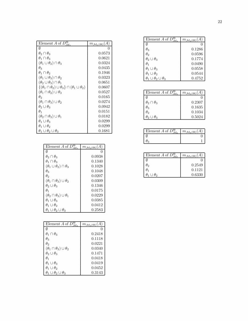
The following table shows the results obtained by the DSm hybrid rule of combination before the finalcompression step of all redundant propositions for the DSm hybrid models presented in the previous examples.

Element A of DΘ mM1(A) mM2(A) mM3(A) mM4(A) mM5(A) mM6(A) mM7(A)∅ 0 0 0 0 0 0 0θ1 ∩ θ2 ∩ θ3 0 0 0 0 0 0 0θ2 ∩ θ3 0.0573 0.0573 0 0 0.0573 0 0θ1 ∩ θ3 0.0621 0.0621 0.0621 0 0 0 0(θ1 ∪ θ2) ∩ θ3 0.0324 0.0324 0.0335 0 0.0334 0 0θ3 0.0435 0.0435 0.0460 0.0494 0.0459 0.0494 0θ1 ∩ θ2 0.1946 0 0 0 0 0 0(θ1 ∪ θ3) ∩ θ2 0.0323 0.0365 0 0 0.0365 0 0(θ2 ∪ θ3) ∩ θ1 0.0651 0.0719 0.0719 0 0 0 0{(θ1 ∩ θ2) ∪ θ3} ∩ (θ1 ∪ θ2) 0.0607 0.0704 0.0743 0 0.0764 0 0(θ1 ∩ θ2) ∪ θ3 0.0527 0.0613 0.0658 0.0792 0.0687 0.0792 0θ2 0.0165 0.0207 0.0221 0.0221 0.0207 0 0.0221(θ1 ∩ θ3) ∪ θ2 0.0274 0.0309 0.0340 0.0375 0.0329 0 0.0375θ2 ∪ θ3 0.0942 0.1346 0.1471 0.1774 0.1518 0.1850 0.1953θ1 0.0151 0.0175 0.0175 0.0195 0 0 0.0195(θ2 ∩ θ3) ∪ θ1 0.0182 0.0229 0.0243 0.0295 0.0271 0 0.0295θ1 ∪ θ3 0.0299 0.0385 0.0419 0.0558 0.0489 0.0589 0.0631θ1 ∪ θ2 0.0299 0.0412 0.0452 0.0544 0.0498 0 0.0544θ1 ∪ θ2 ∪ θ3 0.1681 0.2583 0.3143 0.4752 0.3506 0.6275 0.5786

The next tables present the final result of the DSm hybrid rule of combination after the compression step(the merging of all equivalent redundant propositions) presented in previous examples.

22

Element A of DΘM1

mM1(Θ)(A)

∅ 0θ2 ∩ θ3 0.0573θ1 ∩ θ3 0.0621(θ1 ∪ θ2) ∩ θ3 0.0324θ3 0.0435θ1 ∩ θ2 0.1946(θ1 ∪ θ3) ∩ θ2 0.0323(θ2 ∪ θ3) ∩ θ1 0.0651{(θ1 ∩ θ2) ∪ θ3} ∩ (θ1 ∪ θ2) 0.0607(θ1 ∩ θ2) ∪ θ3 0.0527θ2 0.0165(θ1 ∩ θ3) ∪ θ2 0.0274θ2 ∪ θ3 0.0942θ1 0.0151(θ2 ∩ θ3) ∪ θ1 0.0182θ1 ∪ θ3 0.0299θ1 ∪ θ2 0.0299θ1 ∪ θ2 ∪ θ3 0.1681

Element A of DΘM2

mM2(Θ)(A)

∅ 0θ2 ∩ θ3 0.0938θ1 ∩ θ3 0.1340(θ1 ∪ θ2) ∩ θ3 0.1028θ3 0.1048θ2 0.0207(θ1 ∩ θ3) ∪ θ2 0.0309θ2 ∪ θ3 0.1346θ1 0.0175(θ2 ∩ θ3) ∪ θ1 0.0229θ1 ∪ θ3 0.0385θ1 ∪ θ2 0.0412θ1 ∪ θ2 ∪ θ3 0.2583

Element A of DΘM3

mM3(Θ)(A)

∅ 0θ1 ∩ θ3 0.2418θ3 0.1118θ2 0.0221(θ1 ∩ θ3) ∪ θ2 0.0340θ2 ∪ θ3 0.1471θ1 0.0418θ1 ∪ θ3 0.0419θ1 ∪ θ2 0.0452θ1 ∪ θ2 ∪ θ3 0.3143

Element A of DΘM4

mM4(Θ)(A)

∅ 0θ3 0.1286θ2 0.0596θ2 ∪ θ3 0.1774θ1 0.0490θ1 ∪ θ3 0.0558θ1 ∪ θ2 0.0544θ1 ∪ θ2 ∪ θ3 0.4752

Element A of DΘM5

mM5(Θ)(A)

∅ 0θ2 ∩ θ3 0.2307θ3 0.1635θ2 0.1034θ2 ∪ θ3 0.5024

Element A of DΘM6

mM6(Θ)(A)

∅ 0θ3 1

Element A of DΘM7

mM7(Θ)(A)

∅ 0θ2 0.2549θ1 0.1121θ1 ∪ θ2 0.6330

23

5.9 DSm hybrid rule versus Dempster’s rule of combination

We discuss and compare here the DSm hybrid rule of combination with respect to the Dempster’s rule ofcombination and its alternative proposed in the literature based on the Dempster-Shafer Theory (DST) frame-work which is frequently adopted in many fusion/expert systems. It is necessary to first recall briefly the basisof the DST [13].

5.9.1 Brief introduction to the DST

The DST starts by assuming an exhaustive and exclusive frame of discernment of the problem under con-sideration Θ = {θ1, θ2, . . . , θn}. This corresponds to the Shafer’s model of the problem. The Shafer’s model isnothing more but the DSm model including all possible exclusivity constraints. The Shafer’s model assumesactually that an ultimate refinement of the problem is possible so that θi are well precisely defined/identifiedin such a way that we are sure that they are exclusive and exhaustive. From this Shafer’s model, a basic beliefassignment (bba) m(.) : 2Θ → [0, 1] associated to a given body of evidence B (also called sometimes corpus ofevidence) is defined by

m(∅) = 0 and∑

A∈2Θ

m(A) = 1 (14)

where 2Θ is called the power set of Θ, i.e. the set of all subsets of Θ. The set of all propositions A ∈ 2Θ

such that m(A) > 0 is called the core of m(.) and is denoted K(m). From any bba, one defines the belief andplausibility functions of A ⊆ Θ as

Bel(A) =∑

B∈2Θ,B⊆A

m(B) (15)

Pl(A) =∑

B∈2Θ,B∩A 6=∅

m(B) = 1 − Bel(A) (16)

5.9.2 The Dempster’s rule of combination

Now let Bel1(.) and Bel2(.) be two belief functions over the same frame of discernment Θ and their cor-responding bba m1(.) and m2(.) provided by two distinct bodies of evidence B1 and B2. Then the combinedglobal belief function denoted Bel(.) = Bel1(.) ⊕ Bel2(.) is obtained by combining the basic belief assignments(called also sometimes information granules in the literature) m1(.) and m2(.) through the following Dempster’srule of combination [m1 ⊕ m2](∅) = 0 and ∀B 6= ∅ ∈ 2Θ,

[m1 ⊕ m2](B) =

∑

X∩Y =B m1(X)m2(Y )

1 −∑

X∩Y =∅ m1(X)m2(Y )(17)

The notation∑

X∩Y =B represents the sum over all X, Y ∈ 2Θ such that X ∩ Y = B. The orthogonal sum

m(.) , [m1 ⊕ m2](.) is considered as a basic belief assignment if and only if the denominator in equation (17)is non-zero. The term k12 ,

∑

X∩Y =∅ m1(X)m2(Y ) is called degree of conflict between the sources B1 and B2.When k12 = 1, the orthogonal sum m(.) does not exist and the bodies of evidences B1 and B2 are said to bein full contradiction. Such a case can arise when there exists A ⊂ Θ such that Bel1(A) = 1 and Bel2(A) = 1.Same kind of trouble can occur also with the Optimal Bayesian Fusion Rule (OBFR) [4, 5].

The DST is attractive for the Data Fusion community because it gives a nice mathematical model for ig-norance and it includes the Bayesian theory as a special case [13] (p. 4). Although very appealing, the DSTpresents some weaknesses and limitations because of its model itself, the theoretical justification of the Demp-ster’s rule of combination but also because of our confidence to trust the result of Dempster’s rule of combinationwhen the conflict becomes important between sources (k12 ր 1).

5.9.3 Alternatives of the Dempster’s rule of combination in the DST framework

The Dempster’s rule of combination has however been a posteriori justified by the Smet’s axiomatic of theTransferable Belief Model (TBM) in [17]. But we must also emphasize here that an infinite number of possiblerules of combinations can be built from the Shafer’s model following ideas initially proposed by Lefevre, Colotand Vannoorenberghe in [12] and corrected here as follows:

24

• one first has to compute m(∅) by

m(∅) ,∑

A∩B=∅

m1(A)m2(B)

• then one redistributes m(∅) on all (A 6= ∅) ⊆ Θ with some given coefficients wm(A) ∈ [0, 1] such that∑

A⊆Θ wm(A) = 1 according to

{

wm(∅)m(∅) → m(∅)

m(A) + wm(A)m(∅) → m(A), ∀A 6= ∅(18)

The particular choice of the set of coefficients wm(.) provides a particular rule of combination. Actually thereexists an infinite number of possible rules of combination. Some rules can be better justified than others de-pending on their ability to or not to preserve the associativity and commutativity properties of the combination.It can be easily shown in [12] that such general procedure provides all existing rules developed in the literaturefrom the Shafer’s model as alternative to the primeval Dempster’s rule of combination depending on the choiceof coefficients w(A). As examples:

• the Dempster’s rule of combination can be obtained from (18) by choosing [12] ∀A 6= ∅

wm(∅) = 0 and wm(A) = m(A)/(1 − m(∅))

• the Yager’s rule of combination is obtained by choosing [19, 12]

wm(Θ) = 1

• the Smets’ rule of combination [16, 12] is obtained by accepting the possibility to deal with bba such thatm(∅) > 0 and thus by choosing

wm(∅) = 1

• with the Lefevre and al. formalism [12] and when m(∅) > 0, the Dubois and Prade’s rule of combination[10, 12] is obtained by choosing

∀A ⊆ P , wm(A) =

∑

A1,A2|A1∪A2=A

A1∩A2=∅m⋆

m(∅

where m⋆ , m1(A1)m2(A2) corresponds to the partial conflicting mass which is assigned to A1 ∪ A2 andwhere P is the set of all subsets of 2Θ on which the conflicting mass is distributed defined by

P , {A ∈ 2Θ | ∃A1 ∈ K(m1), ∃A2 ∈ K(m2), A1 ∪ A2 = A and A1 ∩ A2 = ∅}

The computation of the weighting factors wm(A) of the Dubois and Prade’s rule of combination does notdepend only on propositions they are associated with, but also on belief mass functions which have causethe partial conflicts. Thus the belief mass functions leading to the conflict allow to compute that partof conflicting mass which must be assigned to the subsets of P [12]. The Yager’s rule coincides with theDubois and Prade’s rule of combination when choosing P = {Θ}.

5.9.4 DSm hybrid rule is not equivalent to the Dempster’s rule of combination

In its essence, the DSm hybrid rule of combination is close to the Dubois and Prade’s rule of combinationbut more general and precise because it works on DΘ ⊃ 2Θ and allows us to include all possible exclusivity andnon-existential constraints for the model one has to work with. The advantage of using the DSm hybrid ruleis that it does not require the calculation of weighting factors neither the normalization. The DSm hybrid ruleof combination is definitely not equivalent to the Dempster’s rule of combination as one can easily prove in thefollowing very simple example:

25

Let consider Θ = {θ1, θ2} and the two sources in full contradiction providing the following basic beliefassignments

m1(θ1) = 1 m1(θ2) = 0

m2(θ1) = 0 m2(θ2) = 1

Using the classic DSm rule of combination working with the free DSm model Mf , one gets

mMf (θ1) = 0 mMf (θ2) = 0 mMf (θ1 ∩ θ2) = 1 mMf (θ1 ∪ θ2) = 0

If one forces θ1 and θ2 to be exclusive to work with the Shafer’s model M0, then the Dempster’s ruleof combination can not be applied in this limit case because of the full contradiction of the two sources ofinformation. One gets the undefined operation 0/0. But the DSm hybrid rule can be applied in such limitcase because it transfers the mass of this empty set (θ1 ∩ θ2 ≡ ∅ because of the choice of the model M0) tonon-empty set(s), and one gets:

mM0(θ1) = 0 mM0(θ2) = 0 mM0(θ1 ∩ θ2) = 0 mM0(θ1 ∪ θ2) = 1

This result is coherent in this very simple case with the Yager’s and Dubois-Prade’s rule of combination.

Now let examine the behavior of the numerical result when introducing a small variation ǫ > 0 on initialbasic belief assignments m1(.) and m2(.) as follows:

m1(θ1) = 1 − ǫ m1(θ2) = ǫ and m2(θ1) = ǫ m2(θ2) = 1 − ǫ

As shown on figure 1, limǫ→0 mDS(.), where mDS(.) is the result obtained from the Dempster’s rule ofcombination, is given by

mDS(θ1) = 0.5 mDS(θ2) = 0.5 mDS(θ1 ∩ θ2) = 0 mDS(θ1 ∪ θ2) = 0

This result is very questionable because it assigns same belief on θ1 and θ2 which is more informational thanto assign all the belief to the total ignorance. The assignment of the belief to the total ignorance appears tobe more justified from our point of view because it properly reflects the almost total contradiction between thetwo sources and in such cases, it seems legitimist that the information can be drawn from the fusion. Whenwe apply the DSm hybrid rule of combination (using the Shafer’s model M0), one gets the expected beliefassignment on the total ignorance, i.e. mM0(θ1 ∪ θ2) = 1. The figure below shows the evolution of bba on θ1,θ2 and θ1 ∪ θ2 with ǫ obtained with classical Dempster’s rule and DSm hybrid rule based on Shafer’s model M0

(i.e. θ1 ∩ θ2M0≡ ∅) .

0 0.05 0.1-0.5

0

0.5

1

1.5

ε

m(θ1)

Evolution of m(θ1) with ε

Dempster ruleDSm hybrid rule

0 0.05 0.1-0.5

0

0.5

1

1.5

ε

m(θ2)

Evolution of m(θ2) with ε


0 0.05 0.1-0.5

0

0.5

1

1.5

ε

m(θ1 ∪θ

2)

Evolution of m(θ1 ∪θ

2) with ε


Figure 2: Comparison of Dempster’s rule with the DSm hybrid rule on Θ = {θ1, θ2}

26

6 Dynamic fusionThe DSm hybrid rule of combination presented in this paper has been developed for static problems/models,

but is also directly applicable for easily handling dynamic fusion problems in real time as well, since at eachtemporal change of the models, one can still apply such hybrid rule. If DΘ changes, due to the dynamicity ofthe frame Θ, from time tl to time tl+1, i.e. some of its elements which at time tl were not empty become (or areproved) empty at time tl+1, or vice versa: if new elements, empty at time tl, arise non-empty at time tl+1, thisDSm hybrid rule can be applied again at each change. If Θ tests the same but its set of focal (i.e. non-empty)elements of DΘ increases, then again apply the DSm hybrid rule.

6.1 Example 1

Let’s consider the testimony fusion problem4 with the frame

Θ(tl) , {θ1 ≡ young, θ2 ≡ old, θ3 ≡ white hairs}

with the following two basic belief assignments

m1(θ1) = 0.5 m1(θ3) = 0.5

m2(θ2) = 0.5 m2(θ3) = 0.5

By applying the classical DSm fusion rule, one then gets

mMf (Θ(tl))(θ1∩θ2) = 0.25 mMf (Θ(tl))(θ1∩θ3) = 0.25 mMf (Θ(tl))(θ2∩θ3) = 0.25 mMf (Θ(tl))(θ3) = 0.25

Suppose now that at time tl+1, one knows that young people don’t have white hairs (i.e θ1 ∩ θ3 ≡ ∅). How canwe update the previous fusion result with this new information on the model of the problem ? We solve it withthe DSm hybrid rule, which transfers the mass of the empty sets (imposed by the constraints on the new modelM available at time tl+1) to the non-empty sets of DΘ, going on the track of the DSm classic rule. Using theDSm hybrid rule with the constraint θ1 ∩ θ3 ≡ ∅, one then gets:

mM(θ1 ∩ θ2) = 0.25 mM(θ2 ∩ θ3) = 0.25 mM(θ3) = 0.25

and the mass mM(θ1 ∩ θ3) = 0, because θ1 ∩ θ3 = {young} ∩ {white hairs}M≡ ∅ and its previous mass

mMf (Θ(tl))(θ1 ∩ θ3) = 0.25 is transferred to mM(θ1 ∪ θ3) = 0.25 by the DSm hybrid rule.

6.2 Example 2

Let Θ(tl) = {θ1, θ2, . . . , θn} be a list of suspects and let consider two observers who eyewitness the sceneof plunder at a museum in Bagdad and who testify to the radio and TV the identities of thieves using thebasic beliefs assignments m1(.) and m2(.) defined on DΘ(tl), where tl represents the time of the observation.Afterwards, at time tl+1, one finds out that one suspect, among this list Θ(tl), say θi, could not be a suspectbecause he was on duty in another place, evidence which was certainly confirmed. Therefore he has to be takenoff the suspect list Θ(tl), and a new frame of discernment is resulting Θ(tl+1). If this one changes again, oneapplies again the DSm hybrid of combining of evidences, and so on. This is a typically dynamical examplewhere models change with time and where one needs to adapt fusion results with current model over time. Inthe meantime, one can also take into account new observations/testimonies in the DSm hybrid fusion rule assoon as they become available to the fusion system. If Θ and DΘ diminish (i.e. some of their elements areproven to be empty sets) from time tl to time tl+1, then one applies the DSm hybrid rule in order to transferthe masses of empty sets to the non-empty sets (in the DSm classic rule’s way) getting an updated basic beliefassignment mtl+1|tl

(.). Contrarily, if Θ and DΘ increase (i.e. new elements arise in Θ, and/or new elements in

DΘ are proven different from the empty set and as a consequence a basic belief assignment for them is required),then new masses (from the same or from the other sources of information) are needed to describe these newelements, and again one combines them using the DSm hybrid rule.

4This problem has been proposed to the authors in a private communication by L. Cholvy in 2002.

27

6.3 Example 3

Let consider a fusion problem at time tl characterized by the frame Θ(tl) , {θ1, θ2} and two independentsources of information providing the basic belief assignments m1(.) and m2(.) over DΘ(tl) and assume that attime tl+1 a new hypothesis θ3 is introduced into the previous frame Θ(tl) and a third source of evidence availableat time tl+1 provides its own basic belief assignment m3(.) over DΘ(tl+1) where

Θ(tl+1) , {Θ(tl), θ3} ≡ {θ1, θ2, θ3}

To solve such kind of dynamical fusion problems, we just use the classical DSm fusion rule as follows:

• combine m1(.) and m2(.) at time tl using classical DSm fusion rule to get m12(.) = [m1 ⊕ m2](.) overDΘ(tl)

• because DΘ(tl) ⊂ DΘ(tl+1), m12(.) assigns the combined basic belief on a subset of DΘ(tl+1), it is stilldirectly possible to combine m12(.) with m3(.) at time tl+1 by the classical DSm fusion rule to get thefinal result m123(.) over DΘ(tl+1) given by

mtl+1(.) , m123(.) = [m12 ⊕ m3](.) = [(m1 ⊕ m2) ⊕ m3](.) ≡ [m1 ⊕ m2 ⊕ m3](.)

• eventually apply DSm hybrid rule if some integrity constraints have to be taken into account in the modelM of the problem

This method can be directly generalized to any number of sources of evidences and, in theory, to any struc-tures/dimension of the frames Θ(tl), Θ(tl+1), ... In practice however, due to the huge number of elements ofhyper-power sets, the dimension of the frames Θ(tl), Θ(tl+1), . . . must be not too large. This practical limitationdepends on the computer resources available for the real-time processing. Specific suboptimal implementationsof DSm rule will have to be developed to deal with fusion problems of large dimension.

It is also important to point out here that DSmT can easily deal, not only with dynamical fusion problemsbut with decentralized fusion problems as well working on non exhaustive frames. For example, let considera set of two independent sources of information providing the basic belief assignments m1(.) and m2(.) overDΘ12(tl)={θ1,θ2} and another group of three independent sources of information providing the basic belief as-signments m3(.), m4(.) and m5(.) over DΘ345(tl)={θ3,θ4,θ5,θ6}, then it is still possible to combine all informationin a decentralized manner as follows:

• combine m1(.) and m2(.) at time tl using classical DSm fusion rule to get m12(.) = [m1 ⊕ m2](.) overDΘ12(tl).

• combine m3(.), m4(.) and m5(.) at time tl using classical DSm fusion rule to get m345(.) = [m3⊕m4⊕m5](.)over DΘ345(tl).

• consider now the global frame Θ(tl) , {Θ12(tl), Θ345(tl)}.

• eventually apply DSm hybrid rule if some integrity constraints have to be taken into account in the modelM of the problem.

Note that this static decentralized fusion can also be extended to decentralized dynamical fusion also bymixing two previous approaches.

One can even combine all five masses together by extending the vectors mi(.), 1 ≤ i ≤ 5, with null compo-nents for the new elements arisen from enlarging Θ to {θ1, θ2, θ3, θ4, θ5} and correspondingly enlarging DΘ, andusing the DSm hybrid rule for k = 5. And more general combining the masses of any k ≥ 2 sources.

We give now several simple numerical examples for such dynamical fusion problems involving non exclusiveframes.

28

6.3.1 Example 3.1

Let consider Θ(tl) , {θ1, θ2} and the two following basic belief assignments available at time tl:

m1(θ1) = 0.1 m1(θ2) = 0.2 m1(θ1 ∪ θ2) = 0.3 m1(θ1 ∩ θ2) = 0.4

m2(θ1) = 0.5 m2(θ2) = 0.3 m2(θ1 ∪ θ2) = 0.1 m2(θ1 ∩ θ2) = 0.1

The classical DSm rule of combination gives

m12(θ1) = 0.21 m12(θ2) = 0.17 m12(θ1 ∪ θ2) = 0.03 m12(θ1 ∩ θ2) = 0.59

Now let consider at time tl+1 the frame Θ(tl+1) , {θ1, θ2, θ3} and a third source of evidence with thefollowing basic belief assignment

m3(θ3) = 0.4 m3(θ1 ∩ θ3) = 0.3 m3(θ2 ∪ θ3) = 0.3

Then the final result of the fusion is obtained by combining m3(.) with m12(.) by the classical DSm rule ofcombination. One thus obtains:

m123(θ1 ∩ θ2 ∩ θ3) = 0.464 m123(θ2 ∩ θ3) = 0.068 m123(θ1 ∩ θ3) = 0.156 m123((θ1 ∪ θ2) ∩ θ3) = 0.012

m123(θ1 ∩ θ2) = 0.177 m123(θ1 ∩ (θ2 ∪ θ3)) = 0.063 m123(θ2) = 0.051 m123((θ1 ∩ θ3) ∪ θ2) = 0.009

6.3.2 Example 3.2

Let consider Θ(tl) , {θ1, θ2} and the two previous following basic belief assignments m1(.) and m2(.)available at time tl. The classical DSm fusion rule gives gives as before

m12(θ1) = 0.21 m12(θ2) = 0.17 m12(θ1 ∪ θ2) = 0.03 m12(θ1 ∩ θ2) = 0.59

Now let consider at time tl+1 the frame Θ(tl+1) , {θ1, θ2, θ3} and the third source of evidence as in previousexample with the basic belief assignment

m3(θ3) = 0.4 m3(θ1 ∩ θ3) = 0.3 m3(θ2 ∪ θ3) = 0.3

The final result of the fusion obtained by the classical DSm rule of combination corresponds to the result of theprevious example, but suppose now one finds out that the integrity constraint θ3 = ∅ holds, which implies alsoconstraints θ1 ∩ θ2 ∩ θ3 = ∅, θ1 ∩ θ3 = ∅, θ2 ∩ θ3 = ∅ and (θ1 ∪ θ2) ∩ θ3 = ∅. This is the DSm hybrid modelM under consideration here. We then have to readjust the mass m123(.) of the previous example by the DSmhybrid rule and one finally gets

mM(θ1) = 0.147

mM(θ2) = 0.060 + 0.119 = 0.179

mM(θ1 ∪ θ2) = 0 + 0 + 0.021 = 0.021

mM(θ1 ∩ θ2) = 0.240 + 0.413 = 0.653

Therefore, when we restrain back θ3 = ∅ and apply the DSm hybrid rule, we don’t get back the same result(i.e. mM(.) 6= m12(.)) because still remains some information from m3(.) on θ1, θ2, θ1 ∪ θ2, or θ1 ∩ θ2, i.e.m3(θ2) = 0.3 > 0.

29

6.3.3 Example 3.3

Let consider Θ(tl) , {θ1, θ2} and two previous following basic belief assignments m1(.) and m2(.) availableat time tl. The classical DSm fusion rule gives as before

m12(θ1) = 0.21 m12(θ2) = 0.17 m12(θ1 ∪ θ2) = 0.03 m12(θ1 ∩ θ2) = 0.59

Now let consider at time tl+1 the frame Θ(tl+1) , {θ1, θ2, θ3, θ4} and another third source of evidence withthe following basic belief assignment

m3(θ3) = 0.5 m3(θ4) = 0.3 m3(θ3 ∩ θ4) = 0.1 m3(θ3 ∪ θ4) = 0.1

Then, the DSm rule applied at time tl+1 provides the following combined belief assignment

m123(θ1 ∩ θ3) = 0.105 m123(θ1 ∩ θ4) = 0.063 m123(θ1 ∩ (θ3 ∪ θ4)) = 0.021 m123(θ1 ∩ θ3 ∩ θ4) = 0.021

m123(θ2 ∩ θ3) = 0.085 m123(θ2 ∩ θ4) = 0.051 m123(θ2 ∩ (θ3 ∪ θ4)) = 0.017 m123(θ2 ∩ θ3 ∩ θ4) = 0.017

m123(θ3 ∩ (θ1 ∪ θ2)) = 0.015 m123(θ4 ∩ (θ1 ∪ θ2)) = 0.009 m123((θ1 ∪ θ2) ∩ (θ3 ∪ θ4)) = 0.003

m123((θ1 ∪ θ2) ∩ (θ3 ∩ θ4)) = 0.003 m123(θ1 ∩ θ2 ∩ θ3) = 0.295 m123(θ1 ∩ θ2 ∩ θ4) = 0.177

m123((θ1 ∩ θ2) ∩ (θ3 ∪ θ4)) = 0.059 m123(θ1 ∩ θ2 ∩ θ3 ∩ θ4) = 0.059

Now suppose at time tl+2 one finds out that θ3 = θ4 = ∅, then one applies the DSm hybrid rule afterre-adjusting the combined belief mass m123(.) by cummulating the masses of all empty sets. Using the DSmhybrid rule, one finally gets:

mtl+2(θ1) = m123(θ1) + {m12(θ1)m3(θ3) + m12(θ1)m3(θ4) + m12(θ1)m3(θ3 ∪ θ4) + m12(θ1)m3(θ3 ∩ θ4)}

= 0 + {(0.21 × 0.5) + (0.21 × 0.3) + (0.21 × 0.1) + (0.21 × 0.1)} = 0.21

mtl+2(θ2) = m123(θ2) + {m12(θ2)m3(θ3) + m12(θ2)m3(θ4) + m12(θ2)m3(θ3 ∪ θ4) + m12(θ2)m3(θ3 ∩ θ4)}

= 0 + {(0.17 × 0.5) + (0.17 × 0.3) + (0.17 × 0.1) + (0.17 × 0.1)} = 0.17

mtl+2(θ1 ∪ θ2) = m123(θ1 ∪ θ2) + {m12(θ1 ∪ θ2)m3(θ3) + m12(θ1 ∪ θ2)m3(θ4)

+ m12(θ1 ∪ θ2)m3(θ3 ∪ θ4) + m12(θ1 ∪ θ2)m3(θ3 ∩ θ4)}

+∑

X1,X2∈{θ3,θ4,θ3∪θ4,θ3∩θ4}

m12(X1)m3(X2)

= 0 + {(0.03 × 0.5) + (0.03 × 0.3) + (0.03 × 0.1) + (0.03 × 0.1)} + {0} = 0.03

mtl+2(θ1 ∩ θ2) = m123(θ1 ∩ θ2) + {m12(θ1 ∩ θ2)m3(θ3) + m12(θ1 ∩ θ2)m3(θ4)

+ m12(θ1 ∩ θ2)m3(θ3 ∪ θ4) + m12(θ1 ∩ θ2)m3(θ3 ∩ θ4)}

= 0 + {(0.59 × 0.5) + (0.59 × 0.3) + (0.59 × 0.1) + (0.59 × 0.1)} = 0.59

Thus we get the same result as for m12(.) at time tl, which is normal.

Remark: note that if the third source of information don’t assign non-null masses to θ1, or θ2 (or to theircombinations using ∪ or ∩ operators), then one obtains the same result at time tl+2 as at time tl as in this ex-ample 3.3, i.e. ml+2(.) = ml(.), when imposing back θ3 = θ4 = ∅. But, if the third source of information assignsnon-null masses to either θ1, or θ2, or to some of their combinations θ1 ∪ θ2 or θ1 ∩ θ2, then when one returnsfrom 4 singletons to 2 singletons for Θ, replacing θ3 = θ4 = ∅ and using the DSm hybrid rule, the fusion resultsat time tl+2 is different from that at time tl, and this is normal because some information/mass is left fromthe third source and is now fusioned with that of the previous sources (as in example 3.2 or in next example 3.4).

30

In general, let’s suppose that the fusion of k ≥ 2 masses provided by the sources B1, B2, ..., Bk has beendone at time tl on Θ(tl) = {θ1, θ2, ..., θn}. At time tl+1 new non-empty elements θn+1, θn+2, . . ., θn+m appear,m ≥ 1, thus

Θ(tl+1) = {θ1, θ2, ..., θn, θn+1, θn+2, . . . , θn+m}

and of course one or more sources (i.e. bodies of evidences) Bk+1, . . ., Bk+l, where l ≥ 1, appear to assignmasses to these new elements.

a) If all these new sources Bk+1, . . ., Bk+l assign null masses to all elements from DΘ(tl+1) which contain intheir structure/composition at least one of the singletons θ1, θ2, . . ., θn, then at time tl+2 if one sets backthe constraints that θn+1 = θn+2 = . . . = θn+m = ∅, then using the DSm hybrid rule, one obtains thesame result as at time tl, i.e. ml+2(.) = ml(.).

b) Otherwise, the fusion at time tl+2 will be different from the fusion at time tl because still remains someinformation/mass from sources Bk+1, . . ., Bk+l on singletons θ1, θ2, . . ., θn or on some elements fromDΘ(tl) which contain at least one of such singletons, information/mass which fusions with the previoussources.

6.3.4 Example 3.4

Let consider Θ(tl) , {θ1, θ2} and the two following basic belief assignments available at time tl:

m1(θ1) = 0.6 m1(θ2) = 0.4 and m2(θ1) = 0.7 m2(θ2) = 0.3

The classical DSm rule of combination gives m12(θ1) = 0.42, m12(θ2) = 0.12 and m12(θ1 ∩ θ2) = 0.46. Nowlet consider at time tl+1 the frame Θ(tl+1) , {θ1, θ2, θ3} and a third source of evidence with the followingbasic belief assignment m3(θ1) = 0.5, m3(θ2) = 0.2 and m3(θ3) = 0.3. Then the final result obtained from theclassical DSm rule of combination is still as before

m123(θ1) = 0.210 m123(θ2) = 0.024 m123(θ1 ∩ θ2) = 0.466 m123(θ1 ∩ θ3) = 0.126

m123(θ2 ∩ θ3) = 0.036 m123(θ1 ∩ θ2 ∩ θ3) = 0.138

Suppose now one finds out that the integrity constraint θ1 ∩ θ3 = ∅ which also implies θ1 ∩ θ2 ∩ θ3 = ∅.This is the DSm hybrid model M under consideration. By applying the DSm hybrid fusion rule, one forcesmM(θ1∩θ3) = 0 and mM(θ1∩θ2∩θ3) = 0 and we transfer m123(θ1∩θ2∩θ3) = 0.138 towards mM((θ1∩θ2)∪θ3)and the mass m123(θ1 ∩ θ3) = 0.126 has to be transferred towards mM(θ1 ∪ θ3). One then gets finally

mM(θ1) = 0.210 mM(θ2) = 0.024 mM(θ1 ∩ θ2) = 0.466 mM(θ2 ∩ θ3) = 0.036

mM((θ1 ∩ θ2) ∪ θ3) = 0.138 mM(θ1 ∪ θ3) = 0.126

6.3.5 Example 3.5

Let consider Θ(tl) , {θ1, θ2} and the two previous basic belief assignments available at time tl as in previousexample, i.e.

m1(θ1) = 0.6 m1(θ2) = 0.4 and m2(θ1) = 0.7 m2(θ2) = 0.3


m12(θ1) = 0.42 m12(θ2) = 0.12 m12(θ1 ∩ θ2) = 0.46

Now let consider at time tl+1 the frame Θ(tl+1) , {θ1, θ2, θ3} and a third source of evidence with the followingbasic belief assignment

m3(θ1) = 0.5 m3(θ2) = 0.2 m3(θ3) = 0.3

Then the final result of the fusion is obtained by combining m3(.) with m12(.) by the classical DSm rule ofcombination. One thus obtains now

m123(θ1) = 0.210 m123(θ2) = 0.024 m123(θ1 ∩ θ2) = 0.466 m123(θ1 ∩ θ3) = 0.126

m123(θ2 ∩ θ3) = 0.036 m123(θ1 ∩ θ2 ∩ θ3) = 0.138

31

But suppose one finds out that the integrity constraint is now θ3 = ∅ which implies necessarily also θ1 ∩ θ3 =θ2 ∩ θ3 = θ1 ∩ θ2 ∩ θ3 ≡ ∅ and (θ1 ∪ θ2) ∩ θ3 = ∅ (this is our new DSm hybrid model M under consideration inthis example). By applying the DSm hybrid fusion rule, one gets finally the non-null masses

mM(θ1) = 0.336 mM(θ2) = 0.060 mM(θ1 ∩ θ2) = 0.604

6.3.6 Example 3.6

Let consider Θ(tl) , {θ1, θ2, θ3, θ4} and the following basic belief assignments available at time tl :{

m1(θ1) = 0.5 m1(θ2) = 0.4 m1(θ1 ∩ θ2) = 0.1

m2(θ1) = 0.3 m2(θ2) = 0.2 m2(θ1 ∩ θ3) = 0.1 m2(θ4) = 0.4


m12(θ1) = 0.15 m12(θ2) = 0.08 m12(θ1 ∩ θ2) = 0.27 m12(θ1 ∩ θ3) = 0.05 m12(θ1 ∩ θ4) = 0.20

m12(θ2 ∩ θ4) = 0.16 m12(θ1 ∩ θ2 ∩ θ3) = 0.05 m12(θ1 ∩ θ2 ∩ θ4) = 0.04

Now assume that at time tl+1 one finds out that θ1 ∩ θ2M≡ θ1 ∩ θ3

M≡ ∅. Using the DSm hybrid rule, one gets:

mM(θ1 ∩ θ2) = mM(θ1 ∩ θ3) = mM(θ1 ∩ θ2 ∩ θ3) = mM(θ1 ∩ θ2 ∩ θ4) = 0

mM(θ1) = m12(θ1) + m2(θ1)m1(θ1 ∩ θ2) + m1(θ1)m2(θ1 ∩ θ3) = 0.15 + 0.03 + 0.05 = 0.23

mM(θ2) = m12(θ2) + m2(θ2)m1(θ1 ∩ θ2) + m1(θ2)m2(θ1 ∩ θ3) = 0.08 + 0.02 + 0.04 = 0.14

mM(θ4) = m12(θ4) + m1(θ1 ∩ θ2)m2(θ4) = 0 + 0.04 = 0.04

mM(θ1 ∩ θ4) = m12(θ1 ∩ θ4) = 0.20

mM(θ2 ∩ θ4) = m12(θ2 ∩ θ4) = 0.16

mM(θ1 ∪ θ2) = m12(θ1 ∪ θ2) + m1(θ1)m2(θ2) + m2(θ1)m1(θ2) + m1(θ1 ∩ θ2)m2(θ1 ∩ θ2) = 0.22

mM(θ1 ∪ θ2 ∪ θ3) = m12(θ1 ∪ θ2 ∪ θ3) + m1(θ1 ∩ θ2)m2(θ1 ∩ θ3) + m2(θ1 ∩ θ2)m1(θ1 ∩ θ3)

+m1(θ1 ∩ θ2 ∩ θ3)m2(θ1 ∩ θ2 ∩ θ3) = 0.01

6.3.7 Example 3.7

Let consider Θ(tl) , {θ1, θ2, θ3, θ4} and the following basic belief assignments available at time tl :{

m1(θ1) = 0.2 m1(θ2) = 0.4 m1(θ1 ∩ θ2) = 0.1 m1(θ1 ∩ θ3) = 0.2 m1(θ4) = 0.1

m2(θ1) = 0.1 m2(θ2) = 0.3 m2(θ1 ∩ θ2) = 0.2 m2(θ1 ∩ θ3) = 0.1 m2(θ4) = 0.3


m12(θ1) = 0.02 m12(θ2) = 0.12 m12(θ1 ∩ θ2) = 0.28 m12(θ1 ∩ θ3) = 0.06 m12(θ4) = 0.03

m12(θ1 ∩ θ4) = 0.07 m12(θ2 ∩ θ4) = 0.15 m12(θ1 ∩ θ2 ∩ θ3) = 0.15

m12(θ1 ∩ θ2 ∩ θ4) = 0.05 m12(θ1 ∩ θ3 ∩ θ4) = 0.07

Now assume that at time tl+1 one finds out that θ1 ∩ θ2M≡ θ1 ∩ θ3

M≡ ∅. Using the DSm hybrid rule, one gets:

mM(θ1 ∩ θ2) = mM(θ1 ∩ θ3) = mM(θ1 ∩ θ2 ∩ θ3) = mM(θ1 ∩ θ2 ∩ θ4) = 0

mM(θ1) = m12(θ1) + m1(θ1)m2(θ1 ∩ θ2) + m2(θ1)m1(θ1 ∩ θ2) + m1(θ1)m2(θ1 ∩ θ3) + m2(θ1)m1(θ1 ∩ θ3) = 0.11



mM(θ1 ∩ θ4) = m12(θ1 ∩ θ4) = 0.07

mM(θ2 ∩ θ4) = m12(θ2 ∩ θ4) = 0.15

mM(θ1 ∪ θ2) = m12(θ1 ∪ θ2) + m1(θ1 ∩ θ2)m2(θ1 ∩ θ2) + m1(θ1)m2(θ2) + m2(θ1)m1(θ2) = 0.12

mM(θ1 ∪ θ3) = m12(θ1 ∪ θ3) + m1(θ1 ∩ θ3)m2(θ1 ∩ θ3) = 0.02

mM(θ1 ∪ θ2 ∪ θ3) = m12(θ1 ∪ θ2 ∪ θ3) + m1(θ1 ∩ θ2)m2(θ1 ∩ θ3) + m2(θ1 ∩ θ2)m1(θ1 ∩ θ3) = 0.05

32

7 Bayesian mixture of DSm hybrid modelsIn the preceding, one has first shown how to combine generalized basic belief assignments provided by k ≥ 2

independent sources of information with the general DSm hybrid rule of combination which deals with allpossible kinds of constraints introduced by the hybrid model of the problem. This approach implicitly assumesthat one knows/trusts with certainty that the model M (usually a DSm hybrid model) of the problem is validand corresponds to the true model. In some complex fusion problems however (static or dynamic ones), onemay have some doubts about the validity of the model M on which is based the fusion because of the natureand evolution of elements of the frame Θ. In such situations, we propose to consider a set of exclusive andexhaustive models {M1,M2, . . . ,MK} with some probabilities {P{M1}, P{M2}, . . . , P{MK}}. We don’t gohere deeper on the justification/acquisition of such probabilities because this is highly dependent on the natureof the fusion problem under consideration. We just assume here that such probabilities are available at anygiven time tl when the fusion has to be done. We propose then to use the Bayesian mixture of combined massesmMi(Θ)(.) i = 1, . . . , K to obtain the final result :

∀A ∈ DΘ, mM1,...,MK(A) =

K∑

i=1

P{Mi}mMi(Θ)(A) (19)

8 ConclusionIn this paper we have extended the DSmT and the classical DSm rule of combination to the case of hybrid

models for the frame of discernment involved in many complex fusion problems. The free-DSm model (whichassumes that none of the elements of the frame is refinable) can be interpreted as the opposite of the Shafer’smodel (which assumes that all elements of the frame are truly exclusive) on which is based the mathematicaltheory of evidence (Dempster-Shafer Theory - DST). Between these two extreme models, there exists actuallymany possible hybrid models for the frames of discernment depending on the real intrinsic nature of elementsof the fusion problem under consideration. For real problems, some elements of the frame of discernment canappear to be truly exclusive whereas some others cannot be considered as fully discernable or refinable. Thispresent research work proposes a new DSm hybrid rule of combination for hybrid-models based on the DSmT.The DSm hybrid rule works in any model and is involved in calculation of mass fusion of any number of sourcesof information, no matter how big is the conflict/paradoxism of sources, and on any frame of discernment(exhaustive or non-exhaustive, with elements which may be exclusive or non-exclusive or both). This is animportant rule since does not require the calculation of weighting factors, neither normalization as other rulesdo, and the transfer of empty-sets’ masses to non-empty sets masses is naturally done following the DSmnetwork architecture which is derived from the DSm classic rule. DSmT together with DSm hybrid rule appearsfrom now on to be a new alternative to classical approaches and to existing combination rules and to be verypromising for the development of future complex (uncertain/incomplete/paradoxical/dynamical) informationfusion systems.

References[1] Dawid A.P., Conditional Independence in statistical theory, Journal of Royal Statistical Society, Serie B.,

Vol. 41, pp. 1-31, 1979.

[2] Dawid A.P., Conditional Independence, 14th Conf. on Uncertainty and Artificial Intelligence, USA, 1998.

[3] Dawid A.P., Conditional Independence, In Encyclopedia of Statistical Science (Update) Volume 3, Wiley,New York, 1999.

[4] Dezert J., Optimal Bayesian fusion of multiple unreliable classifiers, Proc. of Fusion 2001 Conf., Montreal,Canada, Aug. 8-11, 2001.

[5] Dezert J., Combination of paradoxical sources of information within the Neutrosophic framework, Proceed-ings of the First International Conference on Neutrosophics, pp. 22–46., Univ. of New Mexico, GallupCampus, NM, USA, 1-3 Dec. 2001, Xiquan, Phoenix, 2002.

[6] Dezert J., Foundations for a new theory of plausible and paradoxical reasoning, Information & Security, Aninternational Journal, edited by Prof. Tzv. Semerdjiev, CLPP, Bulg. Acad. of Sciences, Vol. 9, 2002.

33

[7] Dezert J., Fondations pour une nouvelle theorie du raisonnement plausible et paradoxal, ONERA Tech.Rep. 1/06769 DTIM, Jan. 2003.

[8] Dezert J., Smarandache F., Partial ordering of hyper-power sets and matrix representation of belief functionswithin DSmT, Proc. of Fusion 2003 Conf., Cairns, Australia, July 8-11, 2003.

[9] Dezert J., Smarandache F., On the generation of hyper-power sets for the DSmT, Proceedings of the 6thInternational Conference on Information Fusion, Cairns, Australia, July 8-11, 2003.

[10] Dubois D., Prade H., Representation and combination of uncertainty with belief functions and possibilitymeasures, Computational Intelligence, Vol. 4, pp. 244-264, 1998.

[11] Fonck P., Conditional Independence in Possibility Theory, Uncertainty and Artificial Intelligence, pp. 221-226, 1994.

[12] Lefevre E., Colot O., Vannoorenberghe P. Belief functions combination and conflict management, Informa-tion Fusion Journal, Elsevier, 2002.

[13] Shafer G., A Mathematical Theory of Evidence, Princeton Univ. Press, Princeton, NJ, 1976.

[14] Shenoy P., Conditional Independence in Valuation-Based Systems, International Journal of Approximatereasoning, VoL. 10, pp. 203-234, 1994.

[15] Smarandache F. (Editor), Proceedings of the First International Conference on Neutrosophics, Univ. ofNew Mexico, Gallup Campus, NM, USA, 1-3 Dec. 2001, Xiquan, Phoenix, 2002.

[16] Smets Ph.,The combination of evidences in the transferable belief model, IEEE Transactions on PatternAnalysis and Machine Intelligence, Vol. 12, no. 5, pp. 447-458, 1990.

[17] Smets Ph., Kennes R., The transferable belief model, Artificial Intelligence, 66(2), pp. 191-234, 1994.

[18] Studeny M., Formal properties of Conditional Independence in Different Calculi of AI, Proc. of EC-SQARU’93, (Clarke K., Kruse R. and Moral S., Eds.), Springer-Verlag, 1993.

[19] Yager R.R., On the Dempster-Shafer framework and new combination rules, Information Sciences, Vol. 41,pp. 93-138, 1987..

[20] Yaghlane B.B., Smets Ph., Mellouli K., Independence and Non-Interactivity in the Transferable BeliefModel, Workshop on Conditional Independence Structure and graphical Models, Eds. F. Matus and M.Studeny, Toronto, CA, 1999.

[21] Yaghlane B.B., Smets Ph., Mellouli K., Belief Function Independence: I The marginal case, InternationalJournal of Approximate Reasoning, Vol. 29, pp. 47-70, 2002.

[22] Yaghlane B.B., Smets Ph., Mellouli K., Belief Function Independence: II conditional case, InternationalJournal of Approximate Reasoning, Vol. 31, pp. 31-75, 2002.

combining uncertain and paradoxical evidences for dsm hybrid models

Documents