comenius university in bratislava faculty of...
TRANSCRIPT

COMENIUS UNIVERSITY IN BRATISLAVA
FACULTY OF MATHEMATICS, PHYSICS AND INFORMATICS
Decoding the Content of Spatial Working Memory: an fMRI Study
DIPLOMA THESIS
2015 Bc. Richard Dinga

COMENIUS UNIVERSITY IN BRATISLAVA
FACULTY OF MATHEMATICS, PHYSICS AND INFORMATICS
Decoding the Content of Spatial Working Memory: an fMRI Study
DIPLOMA THESIS
Study programme: Cognitive Science (Single degree study, master II. deg., full
time form)
Field of Study: 2503 Cognitive Science
Training work place: Department of Applied Informatics
Supervisor: doc. Grega Repovš, Ph.D.
Bratislava 2015 Bc. Richard Dinga


Abstrakt
Cieľom práce bolo spojiť techniky strojového učenia a fMRI a tak dekódovať obsah
priestorovej pracovnej pamäte z aktivity mozgu. Vedľajšie ciele boli lokalizovať oblasti
mozgu, ktorých vzorec zaznamenanej mozgovej aktivity obsahuje informáciu o pozícií
stimulu, a tiež zhodnotiť podstatu tej informácie a porovnať vzorce mozgovej aktivity v
rôznych časových úsekoch. Participanti vykonávali jednoduchú pracovno-pamäťovú úlohu,
a to zapamätať si pozíciu stimulu. Počas vykonávania tejto úlohy, ich mozgová aktivita
bola zaznamenávaná funkčnou magnetickou rezonanciou. Natrénovali sme “support vector
machine“ klasifikátor tak, aby klasifikoval zaznamenanú mozgovú aktivitu podľa pozície
zobrazeného stimulu. Boli sme schopní predpovedať v ktorom zo štyroch kvadrantov sa
zobrazil stimulus, so štatisticky signifikantnou pravdepodobnosťou v troch zo štyroch
zaznamenaných časových úsekoch medzi zobrazením stimulu a odpoveďou. Presnosť
klasifikátora bola štatisticky signifikantne vyššia, ak bol klasifikátor trénovaný a testovaný
na dátach z toho istého časového úseku. To naznačuje prítomnosť mätúceho signálu v
dátach. Lokalizovali sme informatívny vzorec mozgovej aktivity v záhlavnom laloku, čo je
kompatibilné s takzvanými “sensorimotor-recruitment“ modelmi pracovnej pamäti, ktoré
predpokladajú uchovávanie pamäťovej informácie v tých istých oblastiach, v ktorých je
spracovávaná senzorická informácia. Nenašli sme informatívne vzory aktivity v iných
oblastiach, ktoré sú v literatúre tiež spájané s pracovnou pamäťou, ako je prefrontálna kôra
a záhlavný lalok. Dizajn experimentu nám nedovolil rozlíšiť medzi signálom vzťahujúcim
sa k pracovnej pamäti a signálmi, ktoré sa vzťahujú k iným kognitívnym procesom, ako je
vnímanie alebo pozornosť.
Kľúčové slová: fMRI, MVPA, strojové učenie, pracovná pamäť, priestorová pracovná
pamäť

Abstract
The goal of the thesis was to combine machine learning techniques and fMRI to decode the
content of the spatial working memory from the recorded brain activity. Secondary goals
were to localize brain areas in which pattern of activity carry information about the
stimulus and evaluate nature of that representation and compare informative patterns of
activities over time. Participants performed simple working memory task of remembering
the position of a stimulus during which their brain activity was recorded by fMRI. We
trained a support vector machine classifier to classify brain activities in respect to the
position of the showed stimulus. We were able to decode in which of the 4 quadrants
stimulus appeared with statistically significantly higher than chance level accuracy for 3
out of 4 recorded time points between stimulus presentation and response. Accuracy rate
was statistically significantly higher if the classifier was tested on the data at the same time
point as it was trained on. This suggests confounding signal in the data. We localized
informative pattern of brain activity in the occipital lobe. This is compatible with the
sensorimotor-recruitment models of working memory, which hypothesize that the working
memory information is stored in the same areas that process the sensory information. We
did not find informative patterns of activities in other areas that are often connected to the
storage of working memory content in the literature – namely prefrontal and parietal
cortex. Experimental design did not allow us to distinguish between the signal that is
related to working memory processes and the signal that is related to different cognitive
processes such as perception or attention.
Keywords: fMRI, MVPA, machine learning, working memory, spatial working memory

Table of Contents 1 Introduction .................................................................................................................... 7
1.1 Interdisciplinarity of the study ..................................................................................... 7
1.2 Functional MRI ............................................................................................................ 9
1.2.1 Comparison to other methods ............................................................................. 10
1.3 Multi-variate pattern analysis ..................................................................................... 11
1.3.1 Introduction ......................................................................................................... 11
1.3.2 Loss of information using univariate methods ................................................... 11
1.3.3 Possibilities of MVPA ........................................................................................ 13
1.3.4 Classifier selection .............................................................................................. 15
1.4 Working memory ....................................................................................................... 15
1.4.1 Baddeley Hitch model of working memory ....................................................... 16
1.5 Neuroscience of working memory ............................................................................. 20
1.5.1 Sensorimotor recruitment models of working memory ...................................... 20
1.5.2 Neural mechanisms of WM ................................................................................ 21
1.6 Previous WM decoding studies .................................................................................. 21
1.7 Conclusion.................................................................................................................. 23
1.8 Research questions ..................................................................................................... 24
2 Methods ....................................................................................................................... 26
2.1 Task ............................................................................................................................ 26
2.2 Analysis ...................................................................................................................... 28
2.2.1 Preprocessing ...................................................................................................... 28
2.2.2 Predicting stimulus position ................................................................................ 28
2.2.3 Feature selection and classification .................................................................... 29
2.2.4 Cross-validation .................................................................................................. 29
2.2.5 Statistical evaluation ........................................................................................... 29
3 Results .......................................................................................................................... 32
3.1.1 Decoding the WM content from the brain activity ............................................. 32
3.1.2 Comparison of within time-point to between time-point classifications ............ 33
3.1.3 Localization of information ................................................................................ 35
3.1.4 Evaluating nature of encoded information .......................................................... 35
4 Discussion .................................................................................................................... 39
4.1.1 Decoding the WM content from the brain activity ............................................. 39
4.1.2 Comparison of within time-point to between time-point classifications ............ 40
4.1.3 Localization of information ................................................................................ 41
4.1.4 Evaluating nature of encoded information .......................................................... 42
4.2 Limitations of the study and possible improvements ................................................. 43

5 Conclusion ................................................................................................................... 45
6 Bibliography ................................................................................................................ 47

7
1 Introduction
In this thesis, we used powerful imaging technique of fMRI and machine learning to
extract the contents of working memory from participant‟s brain activity. Our primary goal
was to see if solely on the basis of recorded brain activity, we can decode what is stored in
participant‟s working memory, without them telling us. However we were able to use this
method also for examining scientific questions: such as localization of brain regions where
pattern of activity contains information about the stimulus and comparing memory
representations over time.
Working memory is an important set of cognitive processes for our everyday lives. Its use
is not only in short term retention of sensory information, but its correct functioning is
important for other processes, such as language comprehension, reasoning and planning.
It‟s also tightly connected with other important processes as attention, control or even
consciousness. Its importance is underlined by observed connection of impairments in
working memory and psychiatric disorders. (Constantinidis & Wang, 2004; Baddeley A. ,
2012)
1.1 Interdisciplinarity of the study
The goal of the study was to investigate neural processes during WM activity with
utilization of machine learning techniques. It combines disciplines of psychology,
neuroscience and computer science.
Cognitive neuroscience as part of broader discipline of cognitive science, lies as a separate
field between of psychology and neuroscience. Cognitive neuroscientists investigate
questions such as how the cognition is produced by the brain. For this goal, this field
borrows behavioral tests and cognitive theories from psychology and neuroimaging
methods from neuroscience and computational modeling from more theoretically oriented
areas of cognitive science. (Gazzaniga, 2009)
In order to understand a cognitive phenomenon, it is necessary to know how it is
accomplished at the neuronal level. Subsequently, we need to be able to build a
computational model with satisfactory biological plausibility, which would be able to

8
emulate observed behavior. Building a functioning computational model is a crucial part of
testing our theory of cognition. (O‟Reilly, Munakata, Frank, Hazy, & Contributors, 2012)
Our study provides additional information about neural processes related to working
memory and additional constrains for the computational models.
WM is widely studied phenomenon from the point of view of psychology. The most
prominent model – Baddeley Hitch model of working memory, is now more than 40 years
old. It was established by observing patients with various neurological disorders and by
analyzing the performance of healthy people on double task studies (Baddeley A. , 2012).
By behavioral testing of interference of various cognitive tasks, psychologists were able to
build a stable, well tested psychological model of WM, with high predictive power, even
before the cognitive neuroscience got its modern form.
Neuroscientists use imaging techniques, such as fMRI, EEG and PET to find brain areas
and neural mechanisms that would represent components of the WM model.
Computational models are used by psychologist and neuroscientist as well. They are used
as a way of formalizing theories and of coming up with more rigorous descriptions and
predictions.
With strong formalization of our understanding of neurocognitive processes goes along
another benefit of cognitive models: the possibility of simulating lesions, or other
problems. This would allow us to see the effect of such problems that would not be
possible by experimental methods for practical and ethical reasons. Because of that,
computational models can have also a clinical impact. (O‟Reilly, Munakata, Frank, Hazy,
& Contributors, 2012)
Neuroscience can also have impact on computer science by inspiring novel and useful
algorithms. Biology already inspired various approaches to computation in wide ranges of
areas. For example state of the art computer vision programs that use neural networks with
convolutions imitate some aspects of the structure of the cortex. (Russakovsky, et al.,
2014)
Human brain is still performing some tasks better than current computers do. Therefore, by
uncovering mechanisms that drives those processes, we can develop better, biology
inspired systems.

9
WM concept is extensively studied in psychology and this study uses psychological theory
that describes it and the methods of behavioral/cognitive experiments. Knowing how WM
is embodied in the brain can have implications for the psychological theories as well. For
example, finding distinct neural mechanisms for the tasks that were considered to be
processed by the same module, or reversely, finding two supposedly distinct tasks are
using same neural circuits would require additional explanations for psychological models.
Since this study goes beyond classical notion of activity of the area and to the notion of
information content in the area, it can provide additional constrains and information for the
biologically inspired computational models.
From the neuroscience, our study borrows powerful imaging technique of fMRI. Results
can have an implication for our understanding of information processing in the brain and
for involvement of various brain areas in the WM. Studies of this type can have
implications for psychiatry as well. It was shown that WM impairment is also observed in
some psychiatric disorders (e.g. for schizophrenia see Quee, Eling, M., & Hildebrandt,
2011). This might suggest that mechanisms that are responsible for WM are also important
for mental health. Understanding of those mechanisms can help us develop new diagnostic
techniques or treatments. This study, therefore, is highly interdisciplinary in the methods it
uses and in the areas that a research of this type can potentially influence.
1.2 Functional MRI
Functional MRI doesn‟t measure neuronal activity directly, but it measures changes in the
the blood flow related to it. During the neural activity, neurons consume oxygen and
energy. This causes blood vessels to dilate to provide support of the oxygen that is
required. FMRI usually uses so called BOLD (blood oxygen level dependent) contrast. It is
based on the well-researched phenomenon, that oxygenated hemoglobin has different
magnetic properties than deoxygenated (deoxyhemoglobin is paramagnedic and
oxihemoglobin is diamagnetic). Because of that difference, they behave differently in the
magnetic field of MR scanner. Increase of concentration of oxygenated hemoglobin leads
to higher intensity of the signal in MR. (Faro & Mohamed, 2010)
BOLD response is temporaly delayed after the neuronal activity. The signal follows so
called haemodynamic response function.

10
Figure 1: Haemodynamic response function
Signal peaks around 5 seconds after the neuronal activity and then it slowly goes back to
normal. This slow effect with relatively sparse temporal acquisition of the scans (usually 2-
3 seconds) is the reason for the low temporal resolution of the fMRI in comparison to some
of the other method. Signal change is caused by the difference between increased blood
flow to the area and actual oxygen consumption in the said area. The oxygen flowing to the
area is more than the amount that is consumed. (Faro & Mohamed, 2010)
1.2.1 Comparison to other methods
EEG has an advantage over fMRI in the sense that it has much higher temporal resolution
(milliseconds in comparison to seconds). Also EEG measures neural activity directly – it
measures electrical fields produced by active neurons. FMRI, in contrast, measures related
metabolic changes. However, electrical fields are easily distorted on the way from neurons
to the electrodes on the scalp. Therefore spatial resolution is much lower and is limited to
the upper layers of cortex. (Bunge & Kahn, 2009)
MEG measures magnetic fields related to the active neurons. Because of the relative
stability of the magnetic fields, it‟s possible to measure neural activity with higher spatial
resolution then EEG with the same temporal resolution and it is also easier to localize the

11
source of the signal. However MEG‟s spatial resolution is still not as good as resolution
from fMRI and its high price does not allow wider use of the method. (Bunge & Kahn, 2009)
FMRI is much less invasive than PET/SPECT that requires participants to drink
radioactive substance. Because of the potential danger, PET/SPECT is not widely used for
research. (Bunge & Kahn, 2009)
1.3 Multi-variate pattern analysis
1.3.1 Introduction
Multi-variate pattern analysis (or multi-voxel pattern analysis, MVPA, decoding, brain
reading) is using pattern recognition/machine learning techniques on the fMRI data. This
way of analyzing data became more and more popular in the recent years. Traditional
univariate methods are looking at the differences of activity of each voxel separately in
respect to the experimental condition. Signal for each individual voxel is modeled and later
spatially smoothed to increase signal-to-noise ratio. Then the average amplitude of the
signal is compared either between the conditions or against the baseline signal. This is
done with the intention of averaging out the noise so that the signal of interest would
remain. However this approach destroys the fine scale information that is obtained in the
area and it makes differentiating between some types of conditions impossible. (Raizada &
Kriegeskorte, 2010; Norman, Polyn, Detre, & Haxby, 2006; Haynes & Rees, 2006)
1.3.2 Loss of information using univariate methods
MVPA, on the other hand, considers the fine scale pattern of activity in the ROI. Spatial
smoothing is usually not applied, or applied only in minimal way, and therefore the fine
scale information is not averaged out and diluted in the bigger region. Spatial pattern of
activations of the individual voxels is taken as an input for a pattern recognition algorithm.
The pattern related to one experimental condition is compared to the pattern related to
another stimulus condition in the same area.
This cannot be done using univariate methods, because univariate methods analyze voxels
individually, one at the time, without considering their interactions. However, differences
between conditions can be represented in the combined activities of voxels instead of the
average of the activity of individual voxels. Therefore only multivariate methods would be

12
able to distinguish between them. (Raizada & Kriegeskorte, 2010; Norman, Polyn, Detre,
& Haxby, 2006; Haynes & Rees, 2006)
Figure 2: effect of spatial smoothing on the resolution of the images. We can see how the
fine details are blurred and noise decrease with higher radius of smoothing. Image
obtained from http://www.brainvoyager.com/
Figure 3: Illustration of higher discriminatory power of multivariate methods. In case A,
classes have different voxel means and are distinguishable by univariate methods. In case
B, activity of individual voxels doesn’t provide necessary information about class of the
stimulus. For successful classification it’s necessary to consider interaction between
voxels. Image from Haynes & Rees (2006)

13
1.3.3 Possibilities of MVPA
Although, there were usages of multivariate methods in the past, a truly seminal study for
the MVPA is considered to be Haxby et al. (2001) study. In this study, Haxby and
colleagues used nearest neighbor classifier to identify category of the presented object
from the pattern of activity in the ventral cortex. After this paper, research with
multivariate methods started to grow rapidly following the developments in machine
learning, and cheaper and more accessible computational power.
Since then, a lot of research has been done with interesting implications for cognitive
science. For example Haynes & and Rees (2005) were able to successfully predict the
orientation of a line from early visual cortex, even in situations when the subjects weren't
consciously aware of the line.
Stimulus relevant cortical pattern of activity is unique for every subject. Therefore the
MVP analysis is usually done within subject. So classifiers are tested on the same subject
as they are trained on. To do between subject classifications is a challenging task; however
work has been done also in this area. Raizada and Connolly (2012) were able to classify
identity of the items between subjects by classifying not voxel patterns of activities but the
representational similarity structure of individual classes. Their algorithm utilizes
similarity of neural responses. For example: woman face is similar to the man‟s face, little
bit less similar to the monkey‟s face and very dissimilar with a chair, regardless of
subject‟s own pattern of activity. Haxby et. al. (2011) performed between subject
classification of movie scenes with accuracy of within subject classification. They did it by
first transforming data to common higher dimensional space of common response
functions.
Very impressive results were provided by Miyawaki, et al. (2008) who didn‟t just classify
the stimuli to the categories based on the neural activity, but they were able to reconstruct
the presented visual image from the previously unseen images. They did it by training
multiple classifiers for set small locations in the visual field and combining their
predictions into one image.

14
Figure 4: Reconstruction of the visual experience from the fMRI data (Miyawaki, et al.,
2008)
Figure 5: reconstruction of dynamic movie clips (Nishimoto, Vu, Naselaris, Benjamini, Yu,
& Gallant, 2011)
Another interesting visual reconstruction was done by Nishimoto (2011) where they were
able to reconstruct dynamic visual experience from watching movie clips. This is a

15
remarkable result due to the slow nature of BOLD response. They did it by modeling the
BOLD signal that is acquired from watching hours of video clips and combining 100 most
probable predictions from 5000 hours of YouTube video clips.
MVPA is also used for medical applications as a means of finding wide range of markers
for neural and psychiatric diseases and their prognosis. For example, Schmaal et. al. (2014)
were able to predict the prognosis of the depressive patients from the fMRI data related to
processing of emotional faces. In another study, Hart et al. (2014) were able to
discriminate ADHD patients from healthy controls. Those applications are promising,
however at the moment doesn‟t have accuracy high enough for clinical purposes.
Another possible application for MVPA is brain-computer interface (BCI). Spatial
resolution of fMRI is superior to EEG and more parts of the brain are accessible by fMRI.
Therefore there are different methods possible for making a BCI. However, size of MR and
its immobility is making classical applications of BCI, like moving a cursor, impractical.
On the other hand, fMRI based BCI can provide on-line feedback of brain activity to the
subject and therefore help patients to control some aspects of emotions, behavior, pain
perception etc. (Raizada & Kriegeskorte, 2010)
1.3.4 Classifier selection
Choosing a correct classifier is often an important task. For fMRI classification, usually the linear
classifiers work best. FMRI data have low signal to noise ratio therefore more complicated
classifiers would just overfit noise in the data. Selection of a classifier is therefore not that crucial
for MVPA or classification accuracy. Better results can be obtained by carefully modeling BOLD
response signal and thoughtful feature selection. Furthermore, to get the best accuracy is often not
the goal of an MVPA study. The goal is simply to show that a certain part of the brain represents
the relevant information; and for that, it is sufficient to show that accuracy is higher than chance
level.
1.4 Working memory
Working memory (WM) is a cognitive system that manipulates and stores information to
be used in different cognitive tasks.
The concept of working memory had developed from short term memory (STM); however
they are related to two distinct phenomena. STM was considered to be a unitary system
that is related only to storing of information. On the other hand, WM refers to a set of

16
processes for storing and actively manipulating information and is divided into several sub-
components with different properties and goals. Several different models were proposed to
explain the long range of experimental findings in regards to WM. (Baddeley, 2012;
Repovs & Baddeley, 2006) In this work, we will focus on Baddeley Hitch model of WM
because it is currently the most prominent in literature.
WM developed as an extension of the Atkinson and Shifrin (1968) model of memory. This
model has three components: sensory memory, short term memory and long term memory.
Baddeley Hitch model extends the STM component by dividing it into additional
subcomponents and connecting it with higher attention and control processes. (Baddeley
A. , 2012)
Figure 6: Atkinson and Shifrin (1968) 3 components model of memory. WM concept
extends the short term memory component of the model.
1.4.1 Baddeley Hitch model of working memory
Baddeley Hitch model of WM divides WM into several subsystems based on different
properties of individual components and how the information stored in them interferes with
each other. If the different contents shared the same capacity limitations, then it‟s assumed
that those contents are stored in the same subcomponent and on the other hand, if we can
observe relative independence of contents of different modalities, then it‟s assumed that
they are stored in different subsystems of WM. Research in the area is still going, and
structure of the model can change (as it happened before), but currently Baddeley Hitch
model distinguishes between 4 independent subsystems: phonological loop, visuo-spatial
sketch-pad, episodic buffer and central executive. First three components serve as storage
for information of different modalities and central executive provides higher attention and
control function without its own storage capacity. (Baddeley A. , 2012; Repovs &

17
Baddeley, 2006) Here, we will briefly explain individual subcomponents based on their
apparent behavior and function.
Figure 7: Schema of Baddeley Hitch model of WM from Baddeley (2012). This model
distinguish between ‘Fluid systems’ that use only short term activations and ‘Crystallised
systems’ that represents long term skills and knowledge.
1.4.1.1 Phonological loop
Phonological loop (PL) mainly stores auditory information, but by verbalizing the
stimulus, information of different modalities can be stored in here as well. PL is further
divided to two components: the phonological store and the articulatory control process.
The phonological store can store acoustic or speech-based information for up to 2 seconds.
Articulatory control process can maintain information in the phonological store for a
longer period of time by constantly subvocally repeating it. It can also transform non-
acoustic information to acoustic information in PL by verbalizing it. (Baddeley, 2012;
Baddeley, 2000) This description of PL accounts for the observed effects. For example:
Phonological similarity effect: the sequences of similar sounding letters (B, P, G, T, C, V)
are harder to remember than sequences of acoustically dissimilar letters (X, W, K, R, W,
Q). (Baddeley, 2012; Baddeley, 2000)

18
Word length effect: a series of short words is easier to remember than a series of the same
length of longer words. This is because the longer words take more time to rehearse in the
loop; therefore words have more time to be forgotten. (Baddeley, 2012; Baddeley, 2000)
Articulatory suppression effect: When the participants are asked to repeat a single word,
such as „the,‟ they performance will drop and phonological similarity effect will disappear.
This is hypothesized to be because repeating words is preventing the subvocalization.
(Baddeley, 2012; Baddeley, 2000)
There are other observed effects that are not well understood. However they do not
contradict the model. (Baddeley, 2012; Baddeley, 2000)
1.4.1.2 Visuo-spatial sketchpad
Visuo-spatial sketchpad (VSS) is the component of working memory that is supposed to
maintain and manipulate visual and spatial information. VSS is divided into independent
visual and spatial subcomponents with separate stores and separate rehearsal mechanisms
with same resources of central executive. Experiments showed disruptive effects of spatial
tasks on spatial WM, but not on visual WM, and visual interference tasks disrupt visual
WM performance but not spatial WM. This observation with additional findings is
evidence for the division of visuo-spatial WM systems. However they both share resources
of CE. (Repovs & Baddeley, 2006)
Visual WM
Capacity of visual WM for objects is connected to the complexity of those objects. It drops
with the number of distinguishing features for the objects (Alvarez & Cavanagh, 2004). It
is therefore assumed that information is stored as conjunction of features and not in the
form of integrated objects. Features are stored in independent feature specific stores, and
combined and maintained in the form of an object by attentional processes. Encoding to
the visual WM is strongly affected by previous experience (top down) and perceptual
features (bottom up). (Repovs & Baddeley, 2006)
Spatial WM
Spatial WM is a system responsible for storing spatial information – information about
positions and paths. It was showed that active eye movement, but also other body part
19
movements and even imagining or planning of the movement disrupts or interferes with
the spatial WM (Repovs & Baddeley, 2006).
Logie (1995) in Repovs & Baddeley (2006) proposed that this is due to the interference of
rehearsal from spatial WM and extraction of information required for planning and
execution of movements. It is thought that spatial WM shares resources with spatial
attention and oculomotor control. (Repovs & Baddeley, 2006)
1.4.1.3 Central Executive
Central Executive (CE) is a cognitive system that is responsible for focusing, dividing and
switching attention. It was shown that tasks that are not disrupted by articulatory
suppression (e.g chess) can be effectively disrupted by tasks that put high load on CE. For
Alzheimer‟s disease patients, performance on WM tasks significantly drops if they are
doing more than one task at the time, as opposed to healthy controls. This was showed in
the case when the difficulty of the single task was matched to each individual. AD patients
also have problem with switching between tasks, but not with individual WM tasks.
(Baddeley, 2012; Repovs & Baddeley, 2006) CE contains number of separable executive
functions. Those functions are important not only for WM but also for more general
cognitive systems.
1.4.1.4 Episodic buffer
Episodic buffer (EB) is the newest component that was added to the WM model. It was
added to the model to explain problematic parts that the original model didn‟t account for;
namely connection to LTM and connection between individual subsystems. EB is the
limited capacity system, which combines information in PL and VSS into complex,
multimodal information (episodes, scenes), stores them and integrates them with
information in LTM. It integrates information into unitary episodic representation. It also
serves as a temporary store for the CE, which by itself doesn‟t store any information.
(Baddeley, 2000; Repovs & Baddeley, 2006)
Combining multimodal information into episodes and integrating with LTM can explain
chunking effect of WM; a very important and visible effect that couldn‟t be explained by
original model. EB can also explain serial recall for the visual information, which would
otherwise highly exceed VSS capacity. Also the original model has no way of explaining

20
higher performance on phonological task, when words to remember were supported by
visual stimuli because original model didn‟t have a way to connect the two subsystems. It
is assumed that EB is controlled by CE. (Baddeley A. , 2012)
Figure 8: Speculative model of the working memory from Baddeley (2012). This picture
shows possible additional components and possible structure of the WM. It’s speculative,
because much of its components are not confirmed by experiments.
1.5 Neuroscience of working memory
1.5.1 Sensorimotor recruitment models of working memory
There are several models developed based on neuroscientific data. Sensorimotor
recruitment models of WM are based on the premise that systems related to perception of
the stimulus are also systems responsible for short-term retention of the stimulus. For
example, in case of a visual stimulus, visual area of the brain will be responsible for
sensory processing of the stimulus as well as for remembering it. There is not a part of the
brain that is specifically dedicated to memory storage. Instead, information is stored in
highly stimulus specific areas by persistent activation of the sensory representation
themselves. (D‟Esposito & Postle, 2015)
Challenges for these models arise from explaining the limitations of the VSWM based on
number of objects and also number of features. (D‟Esposito & Postle, 2015) Many
evidence for these models came from MVPA research. Levis, Peacock and Postle (2008) in
(D‟Esposito & Postle, 2015) showed that it is possible to decode information from short

21
term memory based on neural activity related to the access to the LTM. This idea suggests
common representation of information on LTM and STM level. It was also showed that
classifier trained only on attention to location can correctly discriminate for motor
preparation and STM recognition and vice versa. Therefore attention, motor intention and
memory retention are provided by the same neural mechanisms. What we treat like
different processes can be identical processes from the point of view of the brain. (Jerde et.
Al., 2012 in (D‟Esposito & Postle, 2015))
1.5.2 Neural mechanisms of WM
It was repeatedly shown that prefrontal cortex (PFC) exhibits persistent activity during
delayed response tasks. This can suggest that at some WM related information is stored in
the PFC by consistent firing of related populations of neurons. However, MVPA has not
yet been able to decode stimulus specific information from the PFC as it did from sensory
areas. For example, if a person is maintaining the image of a line of particular orientation
in their STM, PFC shows activity during the whole delay period but classifier cannot be
successfully trained to recognize the orientation of the stimulus based on PFC activity. It
is, however, possible to train classifier to recognize to orientation based on activity of the
related visual areas, but those areas are not active during the whole delay period. There are
suggestions that changes in synaptic weights are responsible for the WM, however more
research is needed in this area. (D‟Esposito & Postle, 2015)
D‟Esposito & Postle (2015) argues that PFC does not encode stimulus related information,
but more abstract, hierarchical, task relevant information such as goals, rules and necessary
control for doing the task. PFC in that case provides top down modulation of posterior
areas. PFC doesn‟t serve as a buffer to WM subsystems, but it performs the CE function.
This can be summarized by citation of D‟Esposito & Postle (2015): “The operation of
holding information “in” working memory occurs within the same circuits that process that
information in non-mnemonic contexts. For symbolic information, this has been captured
by models of activated semantic LTM. For sensorimotor information, by sensorimotor
recruitment models.”
1.6 Previous WM decoding studies
Harrison and Tong (2009) showed that sustained activity does not predict the stimulus
orientation. However, they were able to decode the orientation of the stimulus from the

22
early visual areas even when the average activity of the region was at the norm. Sensory
areas maintain information even when there is no overall increase in neuronal activity.
Early visual areas can maintain information about the stimulus, even when there is no
stimulus presented. They decoded orientation of one of the two possible stimulus
orientations (25 and 125 degrees). The stimuli were presented consequently; and after the
presentation, one of the stimuli was cued to be remembered. This was done to isolate WM
specific signal from other possible neural processes such as attention or perception.
Christophel, Hebart, & Haynes (2012) did a similar study (with the same experimental
design), but with complex visual stimuli, which cannot be represented semantically or
verbally (circle containing complex mix of colors), instead of line orientations. The goal of
the study was to show the role of the visual, parietal and PFC regions on VWM: whether
the visual content is re-represented in PFC or the visual memory information is represented
in visual areas and PFC just has the role of control or information is stored in higher order
areas of PFC. They used searchlight approach (proposed by Kriegeskorte (2006), is a way
of using MVPA to map stimulus related information in the cortex, by repeatedly doing
MVP analysis on every sphere of given radius in the brain) to localize regions that contain
the stimulus information. They found information in early visual areas and in posterior
parietal cortex (PPC), an area that was not found in Harrison and Tong (2009) study.
However, only visual areas were considered in Harrison and Tong study. There was no
stimulus relevant information in other areas that have higher activity (e.g PFC). Since PPC
is not a primary visual area, this study showed that WM content can be decoded also from
areas that are not directly responsible for sensory processing.
Riggall and Postle (2013), in their study, examined the relationship between information
content and sustained period of activity. They tried to predict direction of the observed
movement. As in previously mentioned studies, they didn‟t find stimulus related
information in the areas with constant higher activity during delay period. They were able
to accurately decode the stimulus identity based on the voxels that reacted to the stimulus,
however without constant delay period activity. Stimulus information was decodable from
the visual areas, however not from PFC or parietal cortex.
Serences, Ester, Vogel, & Awh (2009) showed that memory related pattern of activation
was in the same area that encoded the information. As in previous studies, they showed
that the information can be decoded from the multi-voxel patterns, in the area that doesn‟t

23
show elevated activity. Participants were asked to remember just one feature from multi-
feature object (color or orientation). Early visual areas only represented the remembered
feature during the delay period and not the other one.
Lee, Kravitz and Baker (2013) examined the function of PFC and extrastriate cortex (V3-
V5) in WM. Goal of the study was to examine closely the function of the lateral PFC.
There were suggestions that the lateral PFC doesn‟t store sensory WM information but
rather stores verbal or conceptual WM information. Same visual stimulus was presented,
but the nature of the to-be-remembered information differed: Either visual feature (object
fragment) or category of the object had to be remembered. They showed that there is
information stored in lateral PFC for nonvisual information. Therefore, this study, contrary
to other studies, showed that there is evidence that PFC is capable of control as well as
storage of information. Authors interpret this such that ability to maintain information is a
property of the whole cortex and that the function of brain regions in WM processes is
flexible and depends on the nature of the maintained information.
On the other hand, in another study Sreenivasan, Curtis, & D‟Esposito (2014) showed that
sensory cortex maintains accurate WM information, lateral PFC maintains goal related
variables that modulate information in sensory cortex, however not the sensory
information.
1.7 Conclusion
WM is still a highly researched area with several open questions and seemingly
contradictory results. It is reasonable to say that the sensory areas are relevant also for the
WM retention. However, the role of other areas is still yet to be established. Hot areas of
research are mainly PFC and parietal parts. In the past it was thought to store the WM
information. However MVPA studies repeatedly failed to find the sensory information in
the area. Right now, the function of the PFC is hypothesized to be either higher order
sensory information storage, or attentional and control processes and modulation. It cannot
be claimed that it is not possible to find stimulus specific information in the PFC in the
future, even with more sensitive methods.
Another hot topic of WM research is the nature of information representation in the cortex.
Constant sustained activity in the sensory area is a popular explanation of WM. However,
it was shown that the stimulus related information can be extracted from the area even if

24
there is no constantly elevated activity and also from the areas other than the primary
sensory areas (e.g. PFC, PPC).
1.8 Research questions
Previous studies were able to predict identity of the stimulus in working memory based on
brain activity. There are still open questions about the brain areas that contain WM
information. Following that, we proposed 4 research questions:
1. Decoding the WM content from the brain activity
Is it possible to decode the spatial information about the stimulus stored in the working
memory, from brain activity? Previous studies were able to successfully predict stimulus
identity. However, we used a different type of stimuli. We therefore hypothesize that it is
possible to predict stimulus identity also for the spatial stimulus. Classifier trained on the
fMRI data, will be able to categorize new data, based on the presented stimulus position,
with a statistically significantly higher accuracy than chance level accuracy.
2. Comparison of within time-point to between time-point classifications
Subsequent to the first hypothesis, we hypothesize that the informative pattern of activity
in the beginning of the delay period will be the same as the informative pattern of activity
at the end of it. Therefore it will be possible to train a classifier on the data from the
beginning of the delay period to classify data from the end of the period and vice versa,
without significant decrease of accuracy.
In addition to the first 2 questions about the possibility of predicting stimulus position, we
also investigate the localization of the informative areas in the brain.
3. Localization of information
Which brain areas contain information about the stimulus position? Previous studies found
information in the early visual areas. However, involvement of PFC and parietal cortex is
still unclear. Due to simplicity of our stimulus, we hypothesize to find informative signal in
the visual cortex and not in PFC though parietal cortex is an open research question.
4. Evaluating the nature of encoded information

25
Subsequent to simple localization of the informative parts of the brain, and following the
suggestions of Coutanche (2013), we will examine the nature of the encoded information. What
information is necessary and/or sufficient for decoding the stimulus position? Is it fine-grained
multivariate pattern of activity or average difference of activity of bigger area?

26
2 Methods
We used the data that were collected at University medical center Ljubljana primarily for a
different study of working memory. Data were collected with 3.5T MR scanner. We used
data of 20 adult subjects.
2.1 Task
Participants performed 8 runs of a spatial WM task (Figure 9). The runs differed in the
response condition. There were 4 possible response conditions in total. Participants
performed every response condition in two experimental runs. The order of the response
conditions was A B C D D C B A. In sum, participants performed 144 trials of WM task
during the fMRI scanning. One task trial consisted of four parts: Fixation point (2.5
seconds), stimulus presentation (200 ms), delay period (9.8 seconds) and response (2.5
seconds) with a varying resting period between the trials (15 to 22.5 seconds).
Participants were asked to fixate their view on to the fixation point. After that, stimulus
was briefly presented pseudo-randomly (stimulus was showed same number of times for
every position in every experimental run) on one of the 36 possible locations. It was
located on the circumference of the circle, 10 degrees apart excluding cardinal axes
(Figure 10).
After stimulus presentation, there was a delay period without any stimulation. Depending
on the experimental run, participants responded by one of the 4 possible ways:
Center: after the delay period, a cursor appeared in the center of the screen and participant
moved it to the location of the presented stimulus.
Non-center: the task was the same as center task, but cursor appeared in a random location.
Therefore participant could not anticipate the movement required for making a response,
since random initial location of the cursor makes required response motion direction also
random, therefore unpredictable.
Match: after delay period, two cues appeared. One cue appeared in the position of
previously showed stimulus and other cue appeared on the different position from the
possible stimulus positions. Participant moved cursor to the correct position. Therefore
they didn‟t perform a free recall memory task, but a recognition task.

27
Non-match: It was the same as the match condition, but participant moved the cursor to the
cue at the incorrect location. This condition had the same effect as non-center task: the
required response movement could not be anticipated by the participant.
Figure 9: schema of the experiment design. Sample appeared on the random position.
After delay period participants responded by one of the 4 possible response types.
Response type was same for all the trials in the experimental run, but differed between
runs.

28
Figure 10: Possible positions for the stimulus presentation. Blue dots represent possible
stimulus positions. Lines represent division to the quadrants. We tried to predict in which
quadrant stimulus appeared.
2.2 Analysis
2.2.1 Preprocessing
The following standard preprocessing steps were used on the collected fMRI data: slice-
timing correction, slice intensity normalization, motion correction, normalization to mode
1000 and one step transform from native space to the atlas space using in-house software
developed at Washington University in Saint Louis.
Within experimental runs, voxels were stripped of linear trends and their activity
normalized by z-scoring. These preprocessing steps were done by PyMVPA (Hanke,
Halchenko, Sederberg, Hanson, Haxby, & Pollmann, 2009).
2.2.2 Predicting stimulus position
We divided the possible positions into 4 quadrants (Figure 10) and tried to classify brain
images in respect to in which of the 4 quadrants the position of the stimulus fell. We
performed separate analysis for every time point. Training and testing of the classifier was
done within subject.

29
2.2.3 Feature selection and classification
From the whole brain, we selected only small subset of most informative voxels that we
chose according to ANOVA scoring in respect to target classes. To prevent circularity in
analysis, choosing voxels was done based on the data from the training set, independently
of the testing data so that testing data would not influence the voxel selection.
Additionally, the number of the chosen voxels was selected within its own cross-validation
loop from the following possible numbers: 10, 20, 50, 100, 200, and 400.
On the selected data, we trained a linear support vector machine classifier from the
PyMVPA library with default parameters (C=1 automatically scaled to the norm of the
data, nu=0.5).
2.2.4 Cross-validation
Dataset was naturally divided into 8 experimental runs. Data that are from different
experimental runs are thought to be more independent than the data from the same run.
Therefore we performed leave one run out cross-validation (8-fold cross-validation).
We chose data from 7 experimental runs as training set and remaining 8th
run as a testing
set. We repeated this procedure 8 times, so that data from every run was in the testing set
exactly once. In addition, we also performed another 7-fold cross-validation within every
training set to choose the number of voxels to be selected for the classification. This was
done to avoid a model-selection bias and circularity in the analysis. Obtained mean
classifier accuracy for 8 runs was computed and used for further statistical analysis.
2.2.5 Statistical evaluation
We used one-sample student‟s t-test to evaluated statistical significance of the classifier
accuracy rate by testing mean accuracy rate from every subject against the null hypothesis,
which is the subject will be at chance level, namely 25%.
Comparing beginning to the end of the delay period
Next, to find out if the pattern of activity of the beginning of the delay period is the same
as the pattern from the end of the period and vice versa, we did the similar cross-validation
setup as above, with the difference that the testing set was from a different time point as
the training set. We used 7 experimental runs for training and data from the remaining run
for testing, however from a different time point.

30
We used paired two-sample t-test to test the null hypothesis of equal accuracy means for
the cases when the classifier was tested on the same time-point or a different time-point.
Localizing informative parts of the brain
For localizing information in the brain, we used a different method than the above
described feature selection with classification. Although the aforementioned method has
predictive power, it is not suitable for brain mapping. Small number of selected voxels is
neither visually stimulating nor informative. Since only small number of voxels is selected
before the classification, most of the brain is neglected from further MVP analysis even if
there is encoded information in those areas that are not selected. In addition to this, voxels
are selected with a univariate measure. Hence, they are blind to multivariate information or
small information spread through a bigger area.
For the reasons above, we used a different method for mapping purposes. We used
searchlight (SL) method as proposed by Kriegeskorte, Goebel, & Bandettini (2006). This
method maps the whole brain for information encoded in the spatial pattern of activities.
Searchlight method works as followed: A small sphere of a given radius is chosen. Voxels
that are in the sphere are the inputs to the classifier; and on them, the classical cross-
validational procedure is performed and mean accuracy rate is computed. Mean accuracy
rate is assigned to the voxel at the center of the sphere and this is repeated for every sphere
in the brain, so every voxel is in the center exactly once. By this procedure, whole brain is
mapped for the information content. Brain areas that obtain information would have
significantly higher than chance level accuracy and areas that do not obtain information
would have accuracy around the chance level.
Statistical significance map
For transforming the raw accuracy maps to the statistical significance map, we used a
similar approach as (Lee, Turkeltaub, Granger, & Raizada, 2012). After computing
individual accuracy maps, we first normalized the activity within every map by subtracting
the chance level accuracy (0.25) from every voxel of the map. After this step, we
subtracted mean of the voxel values from every voxel. We did this to normalize accuracy
rates between subjects in respect to every subject‟s own variation.
After normalization, we performed single sample t-test for every voxel. Resulting map is
thresholded by p=0.001 uncorrected and by minimal cluster size of 20 connected voxels.
31
This approach is more conservative than the approach without normalizing. Therefore it
has less probability for false discovery rate (false positive findings). For creating statistical
significance map, we used SPM8 software (http://www.fil.ion.ucl.ac.uk/spm/).
Multivariate patterns versus mean activity
We decided to follow the suggestions of Coutanche (2013) in comparing different types of
representations in the cortex. We performed 3 types of SL and compared the results. First
we performed the normal SL analysis as described above. We then performed the same SL
analysis; but for every SL sphere, we first subtracted the mean activity of the sphere from
all voxels in the sphere. Third we did SL classification only on sphere means. This was
done to examine whether information is encoded in the multivariate pattern of activity, or
in the difference between average activities between the classes.

32
3 Results
3.1.1 Decoding the WM content from the brain activity
We investigated if the working memory content can be decoded from the brain activity.
We trained and tested a classifier for data from every time point of the experimental trial.
We report average accuracy of mean CV accuracy rates of all subjects for every time point
separately.
Accuracy is close to chance level for time points 0, 2.5, 5 and 22.5 seconds from the
beginning of the trial. We find significantly above the chance classification accuracy on the
time points during the delay period. 7.5s (mean=0.55, SD=0.18, p-val<10-5
),
10s(mean=0.49, SD=0.17, p-val=<10-4
), 12.5s(mean=0.42, SD=0.16, p-val<10-3
),
15(mean=0.5, SD=0.14, p-val<10-4
), and significantly above the chance for the response
period: 17.5(mean=0.5, SD=0.14, p-val<10-4
), 20.5(mean=0.43, SD=0.16, p-val<10-3
).
Stimulus is decodable only after 5 seconds of its presentation. This is an expected
byproduct of the haemodynamic response function, which drives BOLD signal and
therefore classification accuracy. BOLD signal slowly grows and is strongest after 5
seconds of the neuronal activity. Therefore it would be surprising to see higher than chance
accuracy on the time point when the stimulus was presented, simply because the HRF
driven BOLD signal didn‟t have enough time to manifest itself in form of higher accuracy
rate. It‟s obvious why the classification accuracy is on the chance level for the time points
before the stimulus presentation. Since the same analysis setup was performed for every
time point, this can also serve as a control for a potential bias. Classification accuracy is on
the chance level for the time points where it is physically impossible to have information.
Therefore, we can assume that accuracy at other points is not caused by some form of
circularity or model selection bias.

33
Figure 11: Figure of classification accuracy rate dependent of trial time. We can see
higher than chance level accuracy for the whole delay period and response period; and
accuracy on the chance level before and right after stimulus presentation. Error bars +/- 1
SD.
3.1.2 Comparison of within time-point to between time-point classifications
We tested if there is a statistically significant difference between classification accuracy
where training and testing was done on the data from the same time-point versus
classification accuracy where testing was done on data from a different time point. We
tested time points 7.5 (time-point A) and 12.5 seconds (time-point B) after the beginning of
the trial. Accuracy rate within time-point A was 0.56 (0.18 SD). Accuracy rate within time-
point B was 0.43 (0.14 SD). Accuracy when classifier was trained on time point A but
tested on time point B was 0.43 (0.15 SD). Vice-versa (trained on B tested on A) accuracy
rate was 0.36 (0.14 SD). In both cases, when the classifier was tested on the same time
point as it was trained, accuracy was higher. To train and test the classifier on the same
time point has higher accuracy then the other option. Training on time point A and testing
on time point A was significantly higher than testing on time point B (paired sample t-test;
p < 0.005). Similarly, training on time point B has higher accuracy when testing on time
34
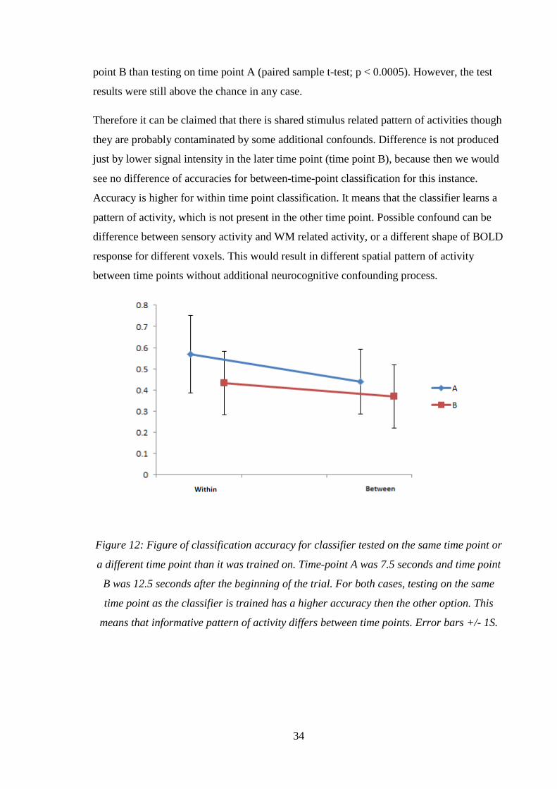
point B than testing on time point A (paired sample t-test; p < 0.0005). However, the test
results were still above the chance in any case.
Therefore it can be claimed that there is shared stimulus related pattern of activities though
they are probably contaminated by some additional confounds. Difference is not produced
just by lower signal intensity in the later time point (time point B), because then we would
see no difference of accuracies for between-time-point classification for this instance.
Accuracy is higher for within time point classification. It means that the classifier learns a
pattern of activity, which is not present in the other time point. Possible confound can be
difference between sensory activity and WM related activity, or a different shape of BOLD
response for different voxels. This would result in different spatial pattern of activity
between time points without additional neurocognitive confounding process.
Figure 12: Figure of classification accuracy for classifier tested on the same time point or
a different time point than it was trained on. Time-point A was 7.5 seconds and time point
B was 12.5 seconds after the beginning of the trial. For both cases, testing on the same
time point as the classifier is trained has a higher accuracy then the other option. This
means that informative pattern of activity differs between time points. Error bars +/- 1S.

35
3.1.3 Localization of information
The approach we used above is not feasible for the mapping of information content to the
brain. Small number of features is selected by univariate measure (ANOVA). Thus
multivariate information of the majority of the cortex is neglected.
In order to find the brain areas that contain stimulus specific information, we used
searchlight approach (Kriegeskorte, Goebel, & Bandettini, 2006). We normalized accuracy
maps within subject by subtracting chance level and mean from every voxel in the
individual subject accuracy map. We then performed one sample t-test for every voxel and
thresholded voxels that exceeds p=0.001 uncorrected and at least clusters of 20 connected
super-threshold voxels.
Clusters of super-threshold voxels were found bilaterally in the occipital cortex.
Figure 13: Results of searchlight analysis for the time point 10 seconds after stimulus
presentation. Clusters of at least 20 connected statistically significant voxels with p <
0.001. Stimulus information can be decoded from visual areas in occipital cortex, but not
from other usually hypothesized areas such as PFC or parietal lobe.
3.1.4 Evaluating nature of encoded information
We evaluated if the information stored in the area is stored in the multivariate pattern of
voxel activities or in the average increase in the activity of the wider area. We did this by
comparing normal searchlight maps against searchlight maps created by subtracting the
mean of the searchlight sphere from the sphere voxels before training and by classifying
only means of the SL spheres.
Accuracy map of the normal SL (Figure 14) and searchlight with mean subtraction (Figure
15) is almost identical, with the same areas with high accuracy rate. This can also be seen
in the Figure 17, where we plotted individual voxel activities and we can see that activities
from normal SL are almost equal to those from the SL with subtracted means. On the other

36
hand, classification of means-only did not produce any bigger informative areas. This
means that information is represented in the multivariate pattern of activity and not in the
difference of mean activity of the bigger area.
Figure 14: the results of the searchlight analysis for the time point 10 seconds after
stimulus presentation. Accuracy map thresholded by 2.5 SD, which was the accuracy rate
of 28.58 percent. We can see that information about the stimulus position is decodable
from the occipital lobe/visual areas of the cortex.
Figure 15: searchlight accuracy map obtained by subtracting mean from the SL sphere
before classification. Thresholded by same accuracy rate as in previous figure, 28.58
percent. We can see that the accuracy map is almost identical with that from Figure 10
where there was no subtraction performed before the classification. Therefore mean
activity of the area does not affect classification of activity, but multivariate pattern of
activity does.
37
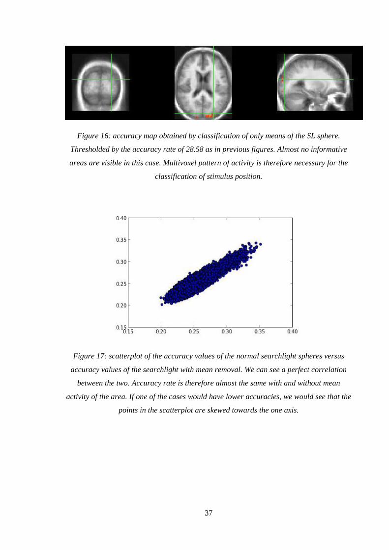
Figure 16: accuracy map obtained by classification of only means of the SL sphere.
Thresholded by the accuracy rate of 28.58 as in previous figures. Almost no informative
areas are visible in this case. Multivoxel pattern of activity is therefore necessary for the
classification of stimulus position.
Figure 17: scatterplot of the accuracy values of the normal searchlight spheres versus
accuracy values of the searchlight with mean removal. We can see a perfect correlation
between the two. Accuracy rate is therefore almost the same with and without mean
activity of the area. If one of the cases would have lower accuracies, we would see that the
points in the scatterplot are skewed towards the one axis.

38
Figure 18: scatterplot of accuracy values of the normal searchlight versus accuracy values
of classification of means only, therefore classification of differences of mean activity in
the area. Accuracy rate of mean classification is lower in magnitude and multitude.

39
4 Discussion
4.1.1 Decoding the WM content from the brain activity
The aim of this part of the study was to predict the position of the presented stimulus from
the activity of the brain recorded by fMRI during the period between stimulus presentation
and participant‟s response. To do this, we selected n (specific number was decided within
additional cross-validation loop) most informative features by ANOVA and trained linear
SVM classifier to discriminate in which of the four quadrants was the stimulus presented.
We tested classification accuracy by 8-fold cross-validation.
We evaluated classification accuracy for every recorded time point of the trial. We were
able to predict the position of the stimulus with statistically significantly higher than
chance accuracy for every time point of the delay period, except the first one, which was
2.5 seconds after stimulus presentation. This observation is in line with the HRF, which
slowly builds up and peaks around 5 seconds after the neural activity. Hence BOLD signal
is just too slow to affect information content in the cortex at the beginning of the delay
period.
Position of the stimulus was decodable from the delay period. Therefore we can say that
the BOLD signal in the cortex contains information about the position of stimulus, either in
spatial or visual form.
This result is in line with previous studies of visual-working memory (e.g. Christophel,
Hebart, & Haynes (2012); Harrison & Tong (2009); Riggal & Postle (2013)), which were
also able to predict the identity of visuo-spatial stimulus from delay period of brain
activity. Our study differs from aforementioned studies in several aspects: we use simple
stimulus - black circle appearing pseudo-randomly appearing on the circumference of the
circle. Previous studies used orientation of the line, complex abstract visual stimulus and
real life objects. For our case what was being remembered is position of the stimulus.
Therefore we aimed to decode spatial information from WM instead of visual. However, it
is impossible to completely disentangle the spatial from visual information. Our spatial
stimulus has a visual property and can also be stored in visual WM. On the other hand
visual stimuli have spatial properties that can be stored in spatial WM as well. Another
difference was that aforementioned studies controlled for the possible confounds related to
the perception. We could not control for this aspect, because the data were primarily

40
collected for a different study and therefore the experimental design was not optimized for
the multivariate decoding of the WM contents.
Therefore we conclude that we are able to predict the position of the stimulus from brain
activity during the delay period. However, additional research is needed to be able to claim
that the decoded information is related to WM and not to other processes.
4.1.2 Comparison of within time-point to between time-point classifications
In the first part of the discussion, we showed that it is possible to predict position of the
presented stimulus from the brain activity during the delay period of a trial, between
stimulus presentation and participant‟s response. Subsequently, we examined if the
patterns of activity during the beginning of the delay period differ from the pattern of
activity in the end of the period. We used similar analysis design as in the first part, but we
tested the training classifier on the data from a different time-point than it was trained on.
We trained linear SVM classifier on the n most informative voxels selected by ANOVA
(number of voxels were determined within additional cross-validation loop) for the time
point of 5 seconds after stimulus presentation and tested the classifier on the time point of
15 seconds after the stimulus presentation. Classifier was always tested on different data
than the data it was trained on. However, in some cases it was tested on the data from a
different time-point than it was trained on.
Classification accuracy was significantly lower, but still higher than chance level accuracy,
when tested on the data from a different time-point than it was trained. We were able to
show that a classifier trained on the data from the beginning of delay period, can predict
position of the stimulus also for the data from the end of the delay period and vice versa. If
trained on the end of the delay period, classifier can also successfully predict stimulus
position from the data at the beginning of the delay period, however with the significantly
lower accuracy.
One possible explanation for this is that the signal is just slowly degrading through the
time course. That would explain the lower accuracy when the classifier is trained in the
first time point and tested on the second. However we observed the degradation of the
accuracy rate also when the classifier was trained on the second time point and was tested
on the first. Because of that, we cannot just assign the observed accuracy rate degradation
to the decay of signal intensity. There needs to be at least one confounding neural process,

41
which needs to also carry the stimulus information. One possibility is that there is a signal
that is related to stimulus perception and another signal that is related to working memory.
They would both carry stimulus information, however with different time course, resulting
in the smaller between-time point accuracy rate. This explanation would challenge the
sensorimotor recruitment models of WM. These models say that the same regions that are
responsible for the perception are also responsible for the WM retention. However this
explanation for the results would assume different circuits processing WM information and
perception.
Another possible explanation would be a change of the WM representation during the time
course of the delay period. For example, from stimulus grounded visual representation in
the beginning to the more abstract, higher-level, spatial representation, at the end of the
delay period. In this scenario, WM would be still produced in the same areas as perception.
However memory consolidation processes would be able to change memory representation
on the voxel level, but still carry stimulus information to explain higher accuracy rate.
One more possibility is that the signal stays about the same level during the whole time
period, but with small, nonrandom fluctuation dependent on different shapes of HRF for
different voxels. This would result in different pattern of activities between time points and
hence higher within time point accuracy rate than between time point accuracy rate. This
explanation is compatible with the sensorimotor recruitment models, because it does not
require different circuits for perception and WM.
In summary, we compared the patterns of activity between different time points of delay
period. Accuracy is higher when classifier is tested on the same time-point as it is trained
on. This can be produced by additional confounding, cognitive or neural phenomena or by
changing of WM representation over time. Experimental design that would control for
additional confounds and modeling of the BOLD signal would be required to answer the
nature of the difference of activity patterns.
4.1.3 Localization of information
We used searchlight approach (Kriegeskorte, Goebel, & Bandettini, 2006) to localize areas
of brain that contain multivariate information about the stimulus position. Searchlight
trains and tests the classifier on every sphere of a given radius in the brain. Resulting
accuracy rate is then assigned for the voxel at the center of the sphere. With this approach,

42
a whole brain is mapped in respect to multivariate information content. We used this
approach to localize the information in the brain, because the method used in the previous
parts of the study is not suitable for brain mapping. In the earlier method voxels were
selected by univariate measures. Therefore in that case, we cannot talk about multivariate
information that is stored in the cortex. In addition to this, a small number of voxels is
selected, most of the brain is neglected for further analysis and thus the resulting
information map would not be informative.
We found statistically significantly above the chance accuracy in the occipital lobe. These
areas are responsible for early visual processing and visual working memory. Stimulus
related information decodable form the visual areas is compatible with previous studies of
visuo-spatial working memory. Christophel, Hebart, & Haynes (2012); Harrison & Tong
(2009); Riggal & Postle (2013) were all able to decode stimulus identity from early visual
areas. However, there are differences to those studies. Christophel, Hebart, & Haynes
(2012), who also used searchlight, found a big cluster of informative voxels on the right
side of the occipital cortex and small cluster on the left side. In our case, whole occipital
lobe was informative without an apparent difference between sides. This can be caused by
a different type of the stimulus – complex abstract visual stimulus versus position of
simple black circle in our case. Our stimulus, in principle was represented in both sides of
the cortex, because it was presented on all sides of the visual field.
As hypothesized, we were not able to decode stimulus position neither from PFC nor from
parietal regions. Lee, Kravitz and Baker (2013) were able to decode information also from
PFC but only for more abstract, nonvisual stimuli. Christophel, Hebart, & Haynes (2012)
found stimulus related information also in parietal cortex. This difference can be explained
by the different stimulus set used in our study.
4.1.4 Evaluating nature of encoded information
Subsequent to the 3rd
research question, we examined the nature of predictive information
stored in the cortex. Specifically, we used different a type of the searchlight classification
to find out if the information is represented in the multivariate pattern of activity, or in the
overall different average of activity of a whole search light sphere.
We found that most of the information was decodable from the multivariate pattern of
activity and not from the mean activity itself. Accuracy rates for the normal searchlight and

43
a searchlight with subtracted mean of the sphere were almost the same. However, the
accuracy rate of classifying only means of sphere activity was significantly lower in terms
of magnitude and size of the informative area. This means that for most part of the found
information, multivariate pattern is necessary and sufficient for decoding the stimulus
position, and mean activity is neither necessary nor sufficient for decoding the stimulus
position. Stimulus position is therefore not represented in the overall higher activity in the
area of the respective part of the cortex, but it‟s represented in more complex spatial
pattern of activity.
4.2 Limitations of the study and possible improvements
We showed that the stimulus position is decodable from the fMRI images from delay
period. However, due to the experimental design, we cannot be certain that the decoded
information is related to the WM processes or to some different confounds, such as
perception, attention or planning. To distinguish between perception and WM related
processes, we would need to adopt a different experimental design. One possibility would
be to use the setup of the previous studies (Christophel, Hebart, & Haynes, 2012; Riggal &
Postle, 2013). In those experiments, two stimuli were presented briefly one after another;
and after their presentation, one of them was cued to be remembered. Because of that,
perception related brain activity should be visible for both stimuli, but WM just only for
the cued one. It is possible to see if a classifier has been learning WM or perception related
information, by comparing classification accuracy of cued stimulus versus not cued one.
Signal that can predict the cued stimulus but not the other should be related to WM
processes. Another possibility would be to show more stimuli at the same time and also
cue just one after the presentation. This would assure that both stimuli will elicit the
perception related neural process, but only one would trigger also WM memory processes.
This setup would also make our second research question - comparison of the beginning of
the delay period to the end of the delay period- more relevant. We showed that the
classification accuracy significantly dropped when the classifier is tested on a different
time point that what it is trained on. However, it was still way above the chance. Therefore
there should be a confounding signal in the data that still carries the stimulus information.
By controlling for the perception related activity, we would get the clearer picture of the
nature of that confound. Another possibility would be to model the signal based on HRF in
order to see what signal trajectories the informative voxels take. We would be able to see if

44
some voxels got active later in the delay period, or if there is only a different path of signal
decay for some of them. There are also different ways of comparing relevant pattern of
activities. One of them is representation similarity analysis (RSA) (Kriegeskorte, Mur, &
Bandettini, 2008), which directly compares similarity of different patterns of activity by
measuring Euclidean distance between patterns of activities of different classes of stimuli.

45
5 Conclusion
In this thesis, we combined functional brain imaging - fMRI and machine learning to
predict the content of spatial working memory and to localize brain areas which carry such
information. We trained a classifier on the fMRI data for the period between stimulus
presentation and a response to classify the position of the stimulus to the one of 4
quadrants. We showed that the classifier could correctly predict the position of the stimulus
on previously unseen data with statistically significantly higher than chance level accuracy.
However, because of the design of the study, we could not distinguish the signal that is
related to the WM processes from the signal that is related to perception or other possible
confounds. Because of that, we concluded that position of the stimulus was decodable from
the fMRI data from the delay period, but we could not certainly tell if we were decoding
WM content, or some other process.
Subsequent to that, we also showed that the pattern of activity that carries information
about stimulus position differs between the beginning and the end of the delay period; and
that the difference cannot be related just to signal decay. We showed this by training and
testing the classifier on the different time point from the delay period and comparing the
accuracy to the accuracy where the testing set was from the same time point. Accuracy was
always higher when tested on the same time point as it was trained on (classifier was
always tested on different set of data. We compared how the accuracy changed if the data
were form the same or different time point). This difference can be produced by additional
confounding effect related to perception of the stimulus. However that would contradict
sensorimotor recruitment models of WM, which assumes same neural circuits involved in
perception to be involved also in WM. According to those models, there should not be a
perception related confounding factor, because signal corresponding to perception should
be in the same voxels that reacts to WM. Possible explanations that are compatible with
sensori-motor recruitment models are: transforming the memory representation during the
delay period, and different BOLD response for different voxels.
We used the searchlight method, to localize brain areas that contain information content
about the stimulus position. Searchlight assesses classification accuracy for every possible
sphere of a given radius in the brain; and by that, maps information content in the cortex.
We found areas of the occipital cortex to be predictable for the stimulus position. This is
compatible with other studies of visuo-spatial working memory. As predicted by sensory-

46
motor recruitment models, we did not find information in other areas usually related to
WM such as PFC and parietal cortex.
Additional analysis with searchlight showed that multivariate pattern of voxels activities,
but not difference in mean activity, is needed for the successful classification of the
stimulus position for the most part of occipital cortex. However, for some small areas,
average activity was also sufficient for higher than chance accuracy, but multivariate
pattern was still more informative.
In summary, we showed that combination of machine learning, neuroscience and
psychology methods could be beneficial for studying the cognitive processes. We used
machine learning techniques to predict the position of the presented stimulus from the
fMRI data, to map the cortex in respect to the information content related to stimulus
position, and to examine the nature of the informative pattern. However, to conclude that
the signal we were able to decode was of the content of WM, we would need to have
different, more controlled experimental design.

47
6 Bibliography
Alvarez, G. a., & Cavanagh. (2004). The Capacity of Visual Short-Term Memory is Set Both by
Visual Information Load and by Number of Objects. Psychological Science, 15(2), 106-111.
Atkinson, R., & Shiffring, R. (1968). Human memory: A proposed system and its control processes.
In K. Spence, & J. Spence, The psychology of learning and motivation (pp. 89-195). New
York: Academic Press.
Baddeley, A. (2000). The episodic buffer: a new component of working memory? Trends in
Cognitive Sciences, 4(11), 417-423.
Baddeley, A. (2012). Working memory: theories, models, and controversies. Anual Review of
Psychology, 63, 1-29.
Bunge, S., & Kahn, I. (2009). Cognition: An overview of neuroimaging techniques. Encyclopedia of
Neuroscience, 2, 1063-1067.
Constantinidis, C., & Wang, X.-J. (2004). A neural circuit basis for spatial working memory. The
Neuroscientist: A Review Journal Bringing Neurobiology, Neurology and Psychiatry, 10(6),
553-565.
Coutanche, M. (2013). Distinguishing multi-voxel patterns and mean activation: why, how, and
what does it tell us. Cognitive, Affective & Behavioural Neuroscience, 13(3), 667-673.
D’Esposito, M., & Postle, B. R. (2015). The Cognitive Neuroscience of Working Memory. Annual
Review of Psychology, 1-28.
Farkas, I. (2012). Indispensability of computational modeling in cognitive science. Journal of
cognitive Science, 1, 401-430.
Faro, S., & Mohamed, F. (2010). BOLD fMRI a guide to functional imaging for neuroscientists. New
York: Springer.
Gazzaniga, M. (2009). Cognitive neuroscience: the biology of the mind. New York: W.W. Norton.
Hanke, M., Halchenko, Y. O., Sederberg, P. B., Hanson, S. J., Haxby, J. V., & Pollmann, S. (2009).
PyMVPA: A python toolbox for multivariate pattern analysis of fMRI data.
Neuroinformatics, 7(1), 37-53.
Harrison, S., & Tong, F. (2009). Decoding reveals the contents of visual working memory in early
visual areas. Nature, 632-635.
Hart, H., Chantiluke, K., Cubillo, A., Smith, A., Simmonds, A., Brammer, M., et al. (2014). Pattern
classification of response inhibition in ADHD: toward the developement of neurobiological
markers for ADHD. Human Brain Mapping, 3083-3094.
Haxby, J. V., Gobbini, M. I., Furey, M. L., Ishai, A., Schouten, J. L., & Pietrini, P. (2001). Distributed
and overlaping representations of faces and objects in ventral temporal cortex. Science,
293(5539), 2425-2430.

48
Haxby, J., Guntupalli, J., Connolly, A., Halchenko, Y. O., Conroy, B. R., Gobbini, I. M., et al. (2011). A
common, high-dimensional model of the representational space in human ventral
temporal cortex. Neuron, 72, 404-416.
Haynes, J., & and Rees, G. (2005). Predicting the orientation of invisible stimuli from activity in
human primary visual cortex. Nature Neuroscience, 686-691.
Haynes, J.-D., & Rees, G. (2006). Decoding mental states from brain activity in humans. Nature
Reviews. Neuroscience, 7(7), 523-34.
Christophel, T. B., Hebart, M. N., & Haynes, J.-D. (2012). Decoding the contents of visual short-
term memory from human visual and parietal cortex. The Journal of Neuroscience, 32(38),
12983-12987.
Kriegeskorte, N., Goebel, R., & Bandettini, P. (2006). Information-based functional brain mapping.
Proccedings of the National Academy of Sciences of the United States of America, 103(10),
3863-3868.
Kriegeskorte, N., Mur, M., & Bandettini, P. A. (2008). Representational similarity analysis -
connecting the branches of systems neuroscience. Frontiers in Systems Neuroscience, 2.
Lee, Y.-S., Turkeltaub, P., Granger, R., & Raizada, R. D. (2012). Categorical speech processing in
Broca's area: an fMRI study using multivariate pattern-based analysis. The Journal of
Neuroscience, 3942-8.
Miyawaki, Y., Uchida, H., Yamashita, O., Sato, M., Morito, Y., Tanabe, H. C., et al. (2008). Visual
image reconstruction from human brain activity using a combintion of multiscale local
image decoders. Neuron, 60(5), 915-29.
Nishimoto, S., Vu, A. T., Naselaris, T., Benjamini, Y., Yu, B., & Gallant, J. L. (2011). Reconstructing
visual experiences from brain activity evoked by natural movies. Current Biology, 21(19),
1641-1646.
Norman, K. a., Polyn, S. M., Detre, G. J., & Haxby, J. V. (2006). Beyond mind-reading: multi-voxel
pattern analysis of fMRI data. Trends in Cognitive Sciences, 424-430.
O’Reilly, R., Munakata, Y., Frank, M., Hazy, T., & Contributors, a. (2012). Computational cognitive
neuroscience (1st Edition ed.). Wiki Book.
Pereira, F., & Botvinick, M. (2010). Information mapping with pattern classifiers: a comparative
study. Neuroimage, 1-37.
Quee, P. J., Eling, P. a., M., v. d., & Hildebrandt, H. (2011). Working memory in schizophrenia: a
systematic study of specific modalities and processes. Psychiatry Research, 185(1-2), 54-
59.
Raizada, R. D., & Kriegeskorte, N. (2010). Pattern-information fMRI: New questions which it opens
up and challenges which face it. International Journal of Imaging Systems and Technology,
20(1), 31-41.

49
Raizada, R., & & Connolly, A. (2012). What makes different people's representations alike: neural
similarity space solves the problem of across-subject fMRI decoding. Journal of Cognitive
Neuroscience, 1-10.
Repovs, G., & Baddeley, A. (2006). The multi-component model of working memory: explorations
in experimental cognitive psychology. Neuroscience, 139(1), 5-21.
Riggal, A., & Postle, B. (2013). Thre realtion between working memory storage and elevated
activity, measured with fMRI. j Neurosci., 32(38), 12990-12998.
Russakovsky, O., Deng, J., Su, H., Krause, J., Satheesh, S., Ma, S., et al. (2014). ImageNet Large
Scale Visual Recognition Challenge, 43. arXiv preprint, 43.
Serences, J., Ester, E., Vogel, E., & Awh, E. (2009). Stimulus-specific delay activity in human
primary visual cortex. Psychological Science, 207-214.
Schmaal, L., Marquand, A. F., Rhebergen, D., van Tol, M.-J., Ruhé, H. G., van der Wee, N. J., et al.
(2014). Predicting the Naturalistic Course of Major Depressive Disorder Using Clinical and
Multimodal Neurological Information: A Multivariate Pattern Recognition Study.
Biological Psychiatry, 1, 1-9.
Sreenivasan, K., Curtis, C., & D’Esposito, M. (2014). Revisiting the role fo presistent neural activity
during working memory. Trends in Cognitive Sciences, 18(2), 82-89.