commercial banking risk management

Commercial Banking Risk Management

Regulation in the Wake of the Financial Crisis

Edited by

Weidong Tian

Weidong TianEditor


Regulation in the Wake of the Financial Crisis

ISBN 978-1-137-59441-9 ISBN 978-1-137-59442-6 (eBook)DOI 10.1057/978-1-137-59442-6

Library of Congress Control Number: 2016961076

© The Editor(s) (if applicable) and The Author(s) 2017This work is subject to copyright. All rights are solely and exclusively licensed by the Publisher, whether the whole or part of the material is concerned, specifically the rights of translation, reprinting, reuse of illustrations, recitation, broadcasting, reproduction on microfilms or in any other physical way, and transmission or information storage and retrieval, electronic adaptation, computer software, or by similar or dissimilar methodology now known or hereafter developed.The use of general descriptive names, registered names, trademarks, service marks, etc. in this publication does not imply, even in the absence of a specific statement, that such names are exempt from the relevant protective laws and regulations and therefore free for general use.The publisher, the authors and the editors are safe to assume that the advice and information in this book are believed to be true and accurate at the date of publication. Neither the pub-lisher nor the authors or the editors give a warranty, express or implied, with respect to the material contained herein or for any errors or omissions that may have been made.

Cover image © PM Images / Getty

Printed on acid-free paper

This Palgrave Macmillan imprint is published by Springer Nature The registered company is Nature America Inc. New York The registered company address is: 1 New York Plaza, New York, NY 10004, U.S.A.

EditorWeidong TianUniversity of North Carolina at CharlotteCharlotte, North Carolina, USA

v

One of the most important lessons from the financial crisis of 2007–2008 is that the regulatory supervision of financial institutions, in particular commercial banks, needs a major overhaul. Many regulatory changes have been implemented in the financial market all over the world. For instance, the Dodd-Frank Act has been signed into federal law on July 2010; the Basel Committee has moved to strengthen bank regulations with Basel III from 2009; the Financial Stability Board created after the crisis has imposed frameworks for the identification of systemic risk in the financial sector across the world; and the Volcker Rule has been adopted formally by financial regulators to curb risk-taking by US commercial banks. Financial institutions have to manage all kinds of risk under stringent regulatory pressure and have entered a virtually new era of risk management.

This book is designed to provide a comprehensive coverage of all impor-tant modern commercial banking risk management topics under the new regulatory requirements, including market risk, counterparty credit risk, liquidity risk, operational risk, fair lending risk, model risk, stress tests, and comprehensive capital analysis and review (CCAR) from a practical perspective. It covers major components in enterprise risk management and a modern capital requirement framework. Each chapter is written by an authority on the relevant subject. All contributors have extensive indus-try experience and are actively engaged in the largest commercial banks, major consulting firms, auditing firms, regulatory agencies and universi-ties; many of them also have PhDs and have written monographs and articles on related topics.

Preface

vi PREFACE

The book falls into eight parts. In Part 1, two chapters discuss regu-latory capital and market risk. Specifically, chapter “Regulatory Capital Requirement in BASEL III” provides a comprehensive explanation of the regulatory capital requirement in Basel III for commercial banks and global systemically important banks. It also covers the current stage of Basel III and the motivations. Chapter “Market Risk Modeling Framework Under Basel” explains the market risk modeling framework under Basel 2.5 and Basel III. The key ingredients are explained and advanced risk measures on the market risk management are introduced in this chapter. The latest capital requirement for the market risk is also briefly documented.

Part 2 focuses on credit risk management, in particular, counter-party credit risk management. Chapter “IMM Approach for Managing Counterparty Credit Risk” first describes the methodologies that have been recognized as standard approaches to tackle counterparty credit risk and, then uses case studies to show how the methodologies are cur-rently used for measuring and mitigating counterparty risk at major com-mercial banks. In the wake of the 2007–2008 financial crisis, one recent challenge in practice is to implement a series of valuation adjustments in the credit market. For this purpose, chapter “XVA in the Wake of the Financial Crisis” presents major insights on several versions of valuation adjustment of credit risks—XVAs, including credit valuation adjustment (“CVA”), debt valuation adjustment (“DVA”), funding valuation adjust-ment (“FVA”), capital valuation adjustment (“KVA”), and margin valua-tion adjustment (“MVA”).

There are three chapters in Part 3. The three chapters each discuss three highly significant areas of risk that are crucial components of the modern regulatory risk management framework. Chapter “Liquidity Risk” docu-ments in detail modern liquidity risk management. It introduces both current approaches and presents some forward-looking perspectives on liquidity risk. After the 2007-2008 financial crisis, the significant role of operational risk has been recognized and operational risk management has emerged as an essential factor in capital stress testing. A modern approach to operational risk management is demonstrated in chapter “Operational Risk Management”, in which both the methodology and several exam-ples of modern operational risk management are discussed. Chapter “Fair Lending Monitoring Models” addresses another key risk management area in commercial banking: fair lending risk. This chapter underscores some of the quantitative challenges in detecting and measuring fair lend-ing risk and presents a modeling approach to it.

PREFACE vii

Part 4 covers model risk management. Built on two well-examined case studies, chapter “Caveat Numerus: How Business Leaders Can Make Quantitative Models More Useful” explains how significant model risk could be, and it presents a robust framework that allows business lead-ers and model developers to understand model risk and improve quan-titative analytics. By contrast, chapter “Model Risk Management Under the Current Environment” provides an extensive discussion about model risk management. In this chapter, model risk management is fully doc-umented, including the methodology, framework, and its management organizational structure. The current challenges frequently encountered in practice and some approaches to address these model risk issues are also presented.

The two chapters in Part 5 concentrate on a major component of the Dodd-Frank Act and Comprehensive Capital Analysis Review (CCAR)-capital stress testing- for commercial banks. Chapter “Region and Sector Effects in Stress Testing of Commercial Loan Portfolio” introduces a gen-eral modeling approach to perform capital stress testing and CCAR in a macroeconomic framework for a large portfolio. Chapter “Estimating the Impact of Model Limitations in Capital Stress Testing” discusses model limitation issues in capital stress testing and presents a “bottom-up” approach to uncertainty modeling and computing the model limitation buffer.

After a detailed discussion on each risk subject in corresponding chap-ter, Part 6 next introduces modern risk management tools. Chapter “Quantitative Risk Management Tools for Practitioners” presents a com-prehensive introduction to quantitative risk management techniques which are heavily employed at commercial banks to satisfy regulatory cap-ital requirements and to internally manage risks. Chapter “Modern Risk Management Tools and Applications” offers an alternative and comple-mentary approach by selecting a set of risk management tools to demon-strate the approaches, methodologies, and usages in several standard risk management problems.

Part 7 addresses another recently emerging important risk manage-ment issue: data and data technology in risk management. Commercial banks and financial firms have paid close attention to risk and regula-tory challenges by improving the use of databases and reporting tech-nology. A widely accepted recent technological solution, Governance, Risk, and Compliance ("GRC"), is explained in greater depth in the two chapters in Part 7. Chapter “GRC Technology Introduction” introduces

viii PREFACE

GRC technology–motivation, principle and framework; chapter “GRC Technology Fundamentals” explains use cases in GRC technology and its fundamentals. Both chapters “GRC Technology Introduction” and “GRC Technology Fundamentals” together provide a comprehensive introduc-tion on the data technology issues regarding many components of risk, including operational risk, fair lending risk, model risk, and systemic risk.

Finally, in the last chapter, chapter “Quantitative Finance in the Post Crisis Financial Environment” (Part 8), current challenges and directions for future commercial banking risk management are outlined. It includes many of the topics covered in previous chapters, for instance, XVAs, oper-ational risk management, fair lending risk management, and model risk management. It also includes topics such as risk of financial crimes, which can be addressed using some of the risk management tools explained in the previous chapters. The list of challenges and future directions is by no means complete; nonetheless, the risk management methodology and appropriate details are presented in this chapter to illustrate these vitally important points and show how fruitful such commercial banking risk management topics could be in the coming times.

Weidong Tian, PhDEditor

ix

I would like to extend my deep appreciation to the contributors of this book: Maia Berkane (Wells Fargo & Co), John Carpenter (Bank of America), Roy E. DeMeo (Wells Fargo & Co), Douglas T. Gardner (Bank of the West and BNP Paribas), Jeffrey R. Gerlach (Federal Reserve of Richmond), Larry Li (JP Morgan Chase), James B. Oldroyd (Brigham Young University), Kevin D. Oden (Wells Fargo & Co), Valeriu (Adi) Omer (Bank of the West), Todd Pleune (Protiviti), Jeff Recor (Grant Thornton), Brain A. Todd (Bank of the West), Hong Xu (AIG), Dong (Tony) Yang (KPMG), Yimin Yang (Protiviti), Han Zhang (Wells Fargo & Co), Deming Zhuang (Citigroup) and Steve Zhu (Bank of America). Many authors have presented in the Mathematical Finance Seminar series of University of North Carolina at Charlotte, and the origins of this book were motivated by organizing these well-designed and insightful presen-tations. Therefore, I would also like to thank the other seminar speak-ers including Catherine Li (Bank of America), Ivan Marcotte (Bank of America), Randy Miller (Bank of America), Mark J. Nowakowski (KPMG), Brayan Porter (Bank of America), Lee Slonimsky (Ocean Partners LP) and Mathew Verdouw (Market Analyst Software), and Stephen D. Young (Wells Fargo & Co).

Many thanks are due to friends and my colleagues at the University of North Carolina at Charlotte. I am particularly indebted to the following individuals: Phelim Boyle, Richard Buttimer, Steven Clark, John Gandar, Houben Huang, Tao-Hsien Dolly King, Christopher M. Kirby, David Li, David Mauer, Steven Ott, C. William Sealey, Jiang Wang, Tan Wang and

acknowledgments

x ACKNOWLEDGMENTS

Hong Yan. Special thanks go to Junya Jiang, Shuangshuang Ji, and Ivanov Katerina for their excellent editorial support.

I owe a debt of gratitude to the staff at Palgrave Macmillan for edi-torial support. Editor Sarah Lawrence and Editorial Assistant Allison Neuburger deserve my sincerest thanks for their encouragement, sugges-tions, patience, and other assistance, which have brought this project to completion.

Most of all, I express the deepest gratitude to my wife, Maggie, and our daughter, Michele, for their love and patience.

xi

Part I Regulatory Capital and Market Risk 1

Regulatory Capital Requirement in Basel III 3Weidong Tian

Market Risk Modeling Framework Under Basel 35Han Zhang

Part II Counterparty Credit Risk 53

IMM Approach for Managing Counterparty Credit Risk 55Demin Zhuang

XVA in the Wake of the Financial Crisis 75John Carpenter

contents

xii CONTENTS

Part III Liquidity Risk, Operational Risk and Fair Lending Risk 101

Liquidity Risk 103Larry Li

Operational Risk Management 121Todd Pleune

Fair Lending Monitoring Models 135Maia Berkane

Part IV Model Risk Management 151

Caveat Numerus: How Business Leaders Can Make Quantitative Models More Useful 153Jeffrey R. Gerlach and James B. Oldroyd

Model Risk Management Under the Current Environment 169Dong (Tony) Yang

Part V CCAR and Stress Testing 199

Region and Sector Effects in Stress Testing of Commercial Loan Portfolio 201Steven H. Zhu

Estimating the Impact of Model Limitations in Capital Stress Testing 231Brian A. Todd, Douglas T. Gardner, and Valeriu (Adi) Omer

CONTENTS xiii

Part VI Modern Risk Management Tools 251

Quantitative Risk Management Tools for Practitioners 253Roy E. DeMeo

Modern Risk Management Tools and Applications 281Yimin Yang

Part VII Risk Management and Technology 303

GRC Technology Introduction 305Jeff Recor and Hong Xu

GRC Technology Fundamentals 333Jeff Recor and Hong Xu

Part VIII Risk Management: Challenge and Future Directions 393

Quantitative Finance in the Post Crisis Financial Environment 395Kevin D. Oden

Index 419

xv

Fig. 1 Capitals, capital ratios, and leverage ratios in Basel III 30Fig. 1 Three components in counterparty risk management

framework 62Fig. 2 Market factors for backtesting 68Fig. 3 An example of backtesting 68Fig. 4 Another example of backtesting 69Fig. 5 Illustration of simulated interest rates in the future dates 70Fig. 6 Prices of the portfolio under the similated scenarios 70Fig. 7 Positive exposure of the portfolio under the simulated

scenarios 71Fig. 8 The expected exposure profile over five years 72Fig. 9 EPE and PFE of 97.7 percentile 72Fig. 1 EPE profile for EUR-USD Cross-currency swap and USD

interest rate swap 81Fig. 2 Funding flows for uncollateralized derivative assets 91Fig. 3 Dealer 1’s received fixed trade flows at execution 97Fig. 4 Dealer 1’s received fixed trade flows after

(mandatory) clearing 98Fig. 1 Overlap in Firmwide Coverage 108Fig. 2 Decision tree 112Fig. 3 Operational balance 114Fig. 4 Business needs break-up 115Fig. 1 Aggregate loss distribution 129Fig. 1 Histogram of Treatment Effect for Different

Matching Methods 146

list of figures

xvi LIST OF FIGURES

Fig. 1 This figure shows the delinquency rate on single-family mortgages and the 10-year Treasury constant maturity rate. Note that the delinquency rate increased sharply during the financial crisis of 2008 even as the Treasury rate continued to decrease, a pattern not consistent with the assumptions of the GRE model 162

Fig. 1 A typical MRM organizational structure 174Fig. 2 MRM framework 181Fig. 3 Model development, implementation and use 183Fig. 4 Model validation structure 187Fig. 1 Partitioning of rating transition matrix 206Fig. 2 Quarterly iteration of estimating credit index Z from default

and transition matrix 208Fig. 3 Historical default rate versus credit index 209Fig. 4 Rho (ρ) and MLE curve as function of (ρ) for selected

industry sector 212Fig. 5 Lead-Lag Relationship between credit index

and GDP growth 214Fig. 6 2013 CCAR scenarios for USA and Europe GDP growth 215Fig. 7 Credit index for North America (NA) under 2013

CCAR SAdv 217Fig. 8 Stress PDs by region and sector across the rating grades 219Fig. 9 Historical downturn PDs compare with CCAR

one year stress PDs 222Fig. 10 Historical downturn PDs compare with CCAR

two year stress PDs 223Fig. 11 Loan loss calculations for first year and second year 225Fig. 12 2012 CCAR loan loss across 18 banks 226Fig. 1 Illustrative example of model developed to forecast

quarterly revenue for a corporate bond brokerage (a) Candidate independent variables are the spread between the yields on the BBB corporate debt and the 10Y US Treasury (BBB; blue line) and the Market Volatility Index (VIX; tan line) (b). Historical data are solid lines and 2015 CCAR severely adverse scenario forecasts are dashed lines. The VIX is chosen as the independent variable in the Model and the BBB is used as the independent variable in the Alt. model 234

LIST OF FIGURES xvii

Fig. 2 Estimating the impact of residual error. The model forecasts quarterly revenue (a) However, it is the error in the nine-quarter cumulative revenue that is most directly related to capital uncertainty (b) The distribution of nine-quarter cumulative errors indicates the expected forecast uncertainty due to residual model error (c) 236

Fig. 3 Estimating the impact of ambiguity in model selection. The performance of the Model (tan) and the Alt. Model (blue) in the development sample are similar (solid lines) (a). The forecasts (dotted lines) are, however, significantly different. The nine-quarter cumulative revenue forecast for the Model (tan dot in (b)) is $45 million greater than the Alt. Model (blue dot in (b)) 239

Fig. 1 GRC Vendor Domain Capabilities 313Fig. 1 Typical GRC Use Cases 334Fig. 2 Example Cyber Security Standard & Regulations Timeline 344Fig. 3 Example GRC Framework 365Fig. 4 Example of an Integrated Control Library 368Fig. 5 Example GRC Integrated Architecture 386

xix

list of tables

Table 1 Interval default probabilities and EPE profiles 82Table 1 Treatment Effect By Strata of Propensity Score 145Table 2 Treatment Effect for Difference Matching Methods 145Table 3 Sensitivity Analysis 146Table 1 S&P historical average transition matrix over 30 years

(1981–2011) 204Table 2 Conditional transition matrix (Z = +1.5 and Z = −1.5) 210Table 3 Stress transition matrix by region projected

for Year 1 and Year 2 220Table 4 2-year transition matrices by selected regions

and industry sectors 221Table 1 Average annual transition matrix 296Table 2 Transition matrix at age one 297Table 3 Transition matrix from 2012 to 2013 297Table 4 Transition matrix from 2013 to 2014 298Table 5 Transition matrix at age three 298Table 6 Transition matrix from 2012 to 2014 298Table 7 Square root transition matrix at age 1/2 299Table 1 Example vendor scoring system 380

xxi

Maia Berkane is a mathematical statistician with extensive experience developing statistical methods for use in finance, psychometrics, and pub-lic health. She taught statistics and mathematics at UCLA and Harvard University. She has been with Wells Fargo since 2007, in asset manage-ment, market risk analytics and, more recently, in regulatory risk manage-ment, as the lead fair lending analytics model developer. Prior to Wells Fargo, she was a quantitative portfolio manager at Deutsch Bank, then Marine Capital, then Credit Suisse, building long/short equity strategies and statistical arbitrage models for trading in the USA and Europe. She holds a PhD in mathematical statistics from Jussieu, Paris VI, France, in the area of extreme value theory.

John Carpenter is a senior currency and interest rate trader in the Corporate Treasury at Bank of America in Charlotte. Prior to joining Bank of America in 2012, he had over ten years of trading experience in New York at Morgan Stanley, Deutsche Bank, and Citigroup across a vari-ety of currency, interest rate, and credit products. John holds an MS in mathematics finance from the Courant Institute at New York University and an MS in computer science from the University of North Carolina at Chapel Hill.

Roy DeMeo has an extensive career in finance, including several business roles at Morgan Stanley, Nomura, Goldman Sachs, and now, Wells Fargo. A highly respected front office modeler whose work has covered equities, interest rate products, FX, commodities, mortgages, and CVA, he is cur-rently a Director, Head of VaR Analytics team, at Wells Fargo, Charlotte.

contributors

xxii CONTRIBUTORS

His current responsibility includes VaR models for volatility skew, specific risk models, and CVA models. His academic background consists of BS in mathematics from MIT, and a PhD in mathematics from Princeton.

Douglas T. Gardner is the Head of Risk Independent Review and Control, Americas, at BNP Paribas, and the Head of Model Risk Management at BancWest. He leads the development and implementation of the model risk management program at these institutions, which includes overseeing the validation of a wide variety of models including those used for enterprise-wide stress testing. He previously led the model risk management function at Wells Fargo and was Director of Financial Engineering at Algorithmics, where he led a team responsible for the development of models used for market and counterparty risk manage-ment. Douglas holds a PhD in Operations Research from the University of Toronto, and was a post-doctoral fellow at the Schulich School of Business, York University.

Jeffrey R. Gerlach is Assistant Vice President in the Quantitative Supervision & Research (QSR) Group of the Federal Reserve Bank of Richmond. Prior to joining the Richmond Fed as a Senior Financial Economist in 2011, Jeff was a professor at SKK Graduate School of Business in Seoul, South Korea, and the College of William & Mary, and an International Faculty Fellow at MIT. He worked as a Foreign Service Officer for the US Department of State before earning a PhD at Indiana University in 2001.

Larry Li is an Executive Director at JP Morgan Chase covering model risk globally across a wide range of business lines, including the corporate and investment bank and asset management. He has around twenty years of quantitative modeling and risk management experience, covering the gamut of modeling activities from development to validation for both valuation models and risk models. Larry is also an expert in market risk, credit risk, and operational risk for the banking and asset management industries. He has previously worked for a range of leading financial firms, such as Ernst & Young, Ospraie, Deutsche Bank, and Constellation Energy. Larry has a PhD in finance and a master’s degree in economics from the University of Toronto. He has also held the GARP Financial Risk Manager certification since 2000.

Kevin D. Oden is an executive vice president and head of Operational Risk and Compliance within Corporate Risk. In his role, he manages

CONTRIBUTORS xxiii

second- line risk activities across information security, financial crimes risk, model risk, operational risk, regulatory compliance risk, and technology risk. He also serves on the Wells Fargo Management Committee. Prior to this he was the Chief Market and Institutional Risk officer for Wells Fargo & Co. and before that, he was the head of Wells Fargo Securities market risk, leading their market risk oversight and model validation, as well as their counterparty credit model development groups. Before joining Wells Fargo in November 2005, he was a proprietary trader at several firms including his own, specializing in the commodity and currency markets. He began his finance career at Goldman Sachs in 1997, working in the risk and commodities groups. Before moving to finance, Kevin was the Benjamin Pierce Assistant Professor of Mathematics at Harvard University, where he specialized in differential geometry and published in the areas of geometry, statistics, and graph theory. Kevin holds a PhD in mathematics from the University of California, Los Angeles and received bachelor degrees in science and business from Cleveland State University.

James Oldroyd is an Associate Professor of Strategy at the Marriott School of Management, Brigham Young University. He received his PhD from the Kellogg School of Management at Northwestern University in 2007. He was an Associate Professor of Management at SKK-GSB in Seoul, South Korea for five years and an Assistant Professor of International Business at Ohio State University for three years. His research explores the intersection of networks and knowledge flows. His work has been pub-lished in outlets such as the Academy of Management Review, Organization Science, and Harvard Business Review. He teaches courses on strategy, organizational behavior, global leadership, leading teams, negotiations, and global business to undergraduates, MBAs, and executives. In addi-tion, to teaching at SKK, OSU, and BYU, he has taught at the Indian School of Business and the University of North Carolina. He is actively involved in delivering custom leadership training courses for numerous companies including Samsung, Doosan, SK, Quintiles, and InsideSales.

Valeriu A. Omer is a Senior Manager in the Model Risk Management Group at Bank of the West. His primary responsibilities consist of oversee-ing the validation of a variety of forecasting models, including those used for capital stress testing purposes, and strengthening the bank’s model risk governance. Prior to his current role, he was a Risk Manager at JPMorgan Chase. Valeriu holds a doctoral degree in economics from the University of Minnesota.

xxiv CONTRIBUTORS

Todd Pleune is a Managing Director at Protiviti, Inc. in Chicago, Illinois. As a leader in the model risk practice of Protiviti’s Data Management and Advanced Analytics Solution, Todd focuses on risk modeling and model validation for operational, market, credit, and interest rate risk. Recently, Todd has supported stress testing model development, validation, and internal audits at major banks. He has developed model governance pro-cesses and risk quantification processes for the world’s largest financial institutions and is an SME for internal audit of the model risk manage-ment function. Todd has a PhD in corrosion modeling from the Massachusetts Institute of Technology, where he minored in finance at the Sloan School of Management and in nuclear physics including stochastic modeling.

Jeff Recor is a Principal at Grant Thornton leading the Risk Technology National Practice. For the past 25 years, Jeff has lead information security efforts for global clients, developing regulatory compliance solutions, information protection programs, assessment and monitoring programs, worked with law enforcement agencies, and implemented security con-trols. Prior to joining Grant Thornton, Jeff created and ran the GRC Technology National Practice at Deloitte for eight years, designing techni-cal solutions to assist clients with enterprise, operational, and information technology risk challenges. Jeff has created several security businesses that were sold to larger organizations, such as a security consulting company which was sold to Nortel in 2000. He has assisted with creating informa-tion security certification programs, supported international standards bodies, helped establish the US Secret Service Electronic Crimes Task Force and also the FBI Infrared program in Michigan, created university- level security curricula, and was chosen as the Information Assurance Educator of the Year by the National Security Agency (NSA).

Weidong Tian is a professor of finance and distinguished professor of risk management and insurance. Prior to coming to UNC Charlotte, Dr. Tian served as a faculty member at the University of Waterloo and a visiting scholar at the Sloan School of Management at MIT. His primary research interests are asset pricing, and derivative and risk management. Dr. Tian has published in many academic journals including Review of Financial Studies, Management Science, Finance and Stochastics, Mathematical Finance, Journal of Mathematical Economics, and Journal of Risk and Insurance. He also published in Journal of Fixed Income and Journal of Investing among others for practitioners. He held various positions in

CONTRIBUTORS xxv

financial institutions before joining the University of Waterloo, and has extensive consulting experience.

Brian A. Todd is a Model Validation Consultant for Bank of the West and the lead developer of the BancWest model limitation buffer used in BancWest's successful 2016 CCAR submission. His other work includes validation of Treasury ALM, Capital Markets, and PPNR models at Bank of the West, BancWest, and BNP Paribas, U.S.A. Inc. Brian was formerly an Assistant Professor of Physics at Purdue University where he led a research group working on exotic diffusion-reaction processes in biologi-cal systems. Brian holds a PhD in Biomedical Engineering from Case Western Reserve University and was a post-doctoral fellow at the National Institutes of Health in Bethesda, Maryland.

Hong Xu is the Global Head of Third Party Risk and Analytics at AIG. He is responsible for establishing a global vendor and business part-ner risk management strategy, process, and technology platform for AIG. Prior to joining AIG, Hong was an SVP at Bank of America for ten years, where he was responsible for service delivery and platform strategy, supporting vendor risk management and strategic sourcing. He also estab-lished a strategic center of excellence for Archer eGRC platform across the enterprise at Bank of America to focus on Archer Solution Delivery. Prior to Bank of America, Hong spent several years with Ariba, a business com-merce company focused on online strategic sourcing and procurement automation. Hong holds an MS in industrial engineering, a BS in mechan-ical engineering, and a six-sigma black belt certification.

Dong (Tony) Yang is a Managing Director of the Risk Consulting ser-vices at KPMG LLP, with extensive business experience in the financial services industry. His focus is on model risk management, quantitative finance, market and treasury risk management, and financial derivatives and fixed-income securities valuation. Tony holds the degrees of master in financial economics and an MBA in finance, as well as various professional certifications, including CFA, CPA, FRM, ERP, and SAS certified advanced programmer for SAS9.

Yimin Yang is a Senior Director at Protiviti Inc. with extensive experi-ence in the risk management area. Prior to his current role, he headed risk analytics teams for PNC Financial Services Group and SunTrust Banks Inc. He holds a bachelor’s degree from Peking University and a PhD from the University of Chicago. He also has a master’s degree in information

xxvi CONTRIBUTORS

networking from Carnegie Mellon University and a master’s degree from the Chinese Academy of Sciences. He taught as a tenure-track assistant professor at University of Minnesota, Morris.

Han Zhang is a Managing Director at Wells Fargo Bank and the head of the Market Risk Analytics Group. He manages the Market Risk Analytics team’s design and implementation as well as monitoring all major market risk capital models (which includes the General VaR model, the debt/equity specific risk model, the stressed VaR/specific risk model and the incremental risk charge model), the counter party and credit risk model, and the economical capital model. Han received his PhD from Shanghai Jiao Tong University (China) in Materials Science, he also has three mas-ter’s degrees in mathematics finance, computer science and mechanical engineering.

Steven H. Zhu is a seasoned quantitative risk and capital market profes-sional with more than twenty years of industry experience. He has worked at Bank of America since 2003 and served in various positions within mar-ket risk and credit risk management, responsible for market risk analysis and stress testing, capital adequacy mandated under the US regulatory reform act (Dodd-Frank). He formerly headed the credit analytics and methodology team at Bank of America securities between 2003 and 2008, responsible for developing risk methodology, credit exposure models, counterparty risk control policy, and related processes to support credit risk management for trading business across various product lines, includ-ing foreign exchange, equity trading, fixed income, and securities financ-ing. He started his career in 1993 at Citibank, New York in derivatives research and trading and he also worked at Citibank Japan office in Tokyo for three years, where he managed the trading book for interest rate/cur-rency hybrid structured derivative transactions. He obtained his PhD in applied mathematics from Brown University, an MS in operation research from Case Western Reserve University and a BS in mathematics from Peking University. He spent 1992–1993 in academic research as a visiting scholar at MIT Sloan School of Management.

Deming Zhuang has been working in the financial industry since 2000. He has worked in different areas of financial risk management, first at Royal Bank of Canada, then at TD Bank, and currently at Citigroup. Deming has worked on counterparty credit exposure model development and IMM model validations. He has a PhD in applied mathematics and an

CONTRIBUTORS xxvii

MS in computer science from Dalhousie University in Canada. Prior to working in the financial industry, Deming held a tenured Associate Professorship at Department of Mathematics and Comptuer Studies at Mount Saint Vincent University from 1989 to 1998. His main research interests were applied nonlinear analysis and numerical optimization. He has published over 20 research papers in refereed mathematics journals.

Regulatory Capital and Market Risk

3© The Author(s) 2017W. Tian (ed.), Commercial Banking Risk Management, DOI 10.1057/978-1-137-59442-6_1

Regulatory Capital Requirement in Basel III

Weidong Tian

W. Tian (*) University of North Carolina at Charlotte, Charlotte, NC, USAe-mail: [email protected]

IntroductIon

The major changes from Basel II (BCBS, “International Convergence of Capital Measurement and Capital Standards: A Revised Framework – Comprehensive Version”, June 2006; “Enhancements to the Basel II framework”, July 2009; “Revisions to the Basel II market risk framework”, July 2009) to Basel III (BCBS, “Basel III: A global regulatory frame-work for more resilient banks and banking systems”, December 2010 (rev. June 2011); BCBS, “Basel III: International framework for liquidity risk measurement, standards and monitoring”) are the shifts largely from risk sensitive to capital intensive in the perspective of risk management.1 By risk sensitive we mean that each type of risk—market risk, credit risk, and operational risk—is being treated separately. These three types of risks are three components of Basel II’s Pillar 1 on Regulatory capital.2 By con-trast, a capital sensitive perspective leads to a more fundamental issue, that of capital, and enforces stringent capital requirements to withstand severe economic and market situations. This capital concept is extended to be total loss-absorbing capacity (TLAC) by the Financial Stability Board (FSB) report of November 2014, “Adequacy of Loss-absorbing Capacity

mailto:[email protected]

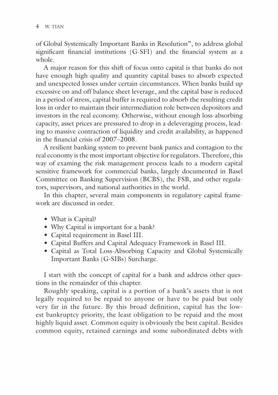
of Global Systemically Important Banks in Resolution”, to address global significant financial institutions (G-SFI) and the financial system as a whole.

A major reason for this shift of focus onto capital is that banks do not have enough high quality and quantity capital bases to absorb expected and unexpected losses under certain circumstances. When banks build up excessive on and off balance sheet leverage, and the capital base is reduced in a period of stress, capital buffer is required to absorb the resulting credit loss in order to maintain their intermediation role between depositors and investors in the real economy. Otherwise, without enough loss-absorbing capacity, asset prices are pressured to drop in a deleveraging process, lead-ing to massive contraction of liquidity and credit availability, as happened in the financial crisis of 2007–2008.

A resilient banking system to prevent bank panics and contagion to the real economy is the most important objective for regulators. Therefore, this way of examing the risk management process leads to a modern capital sensitive framework for commercial banks, largely documented in Basel Committee on Banking Supervision (BCBS), the FSB, and other regula-tors, supervisors, and national authorities in the world.

In this chapter, several main components in regulatory capital frame-work are discussed in order.

• What is Capital?• Why Capital is important for a bank?• Capital requirement in Basel III.• Capital Buffers and Capital Adequacy Framework in Basel III.• Capital as Total Loss-Absorbing Capacity and Global Systemically

Important Banks (G-SIBs) Surcharge.

I start with the concept of capital for a bank and address other ques-tions in the remainder of this chapter.

Roughly speaking, capital is a portion of a bank’s assets that is not legally required to be repaid to anyone or have to be paid but only very far in the future. By this broad definition, capital has the low-est bankruptcy priority, the least obligation to be repaid and the most highly liquid asset. Common equity is obviously the best capital. Besides common equity, retained earnings and some subordinated debts with

4 W. TIAN

long maturity and no covenant to be redeemed (if liquid enough) are also examples of a bank’s capital. However, we have to be very careful to apply this concept due to its complexity.

Let us take a simple example to motivate our explanation below. A bank has $8 million of common equity and takes $92 million of deposits; and the bank has a $100 million of loans outstanding. The loan is on the asset side of the bank’s balance sheet while its liability side consists of deposits and shareholder equity. If the loans perform well, the bank is able to fulfill obligations to the depositors and short-term investors, and makes a profit for the shareholders. The current capital to asset value is 8% if the risk weight to the loan is 10%. If the loan is less risky and its risk weight to the loan is assigned to be 50%, then the capital ratio (following the calculation methodology in Basel I and Basel II) is 16%.

If some losses occurred to the loan, say, $6 million worth of loan was not repaid, then the capital of $8 million can be used to protect the depositors but the capital ratio reduces to 2/94 = 2.15% (assuming the loan’s risk weight is 100%). In this case, $8 million of common equity is a sound and solid capital buffer since it does not have to be repaid in all circumstances, but the capital buffer drops from $8 million to $2 million. Evidently, the $2 million of capital buffer makes the bank very fragile against possible further loss. One way to increase the capital buffer is to issue new equity, say $3 million for new shares. The new capital ratio is (2+3)/(94+3) = 5.15%. But when the market situation is extremely bad, it could be hard for the bank to issue new equity shares, or even in doing so, the new equity share would be issued at a substantial discount; thus, the new capital ratio is smaller than 5.15% in reality.

In another extreme eventuality, a large number of depositors withdraw money at the same time; the bank runs into a mismatch challenge because its asset’s maturing time is much longer than the liability’s maturity. In our example with initial $8 million of common equity, when $5 million is withdrawn simultaneously, the bank is enabled to use $5 million from the capital buffer to pay to the depositor, and the capital buffer drops to $3 million. However, if barely $10 million out of total $92 million of deposits is withdrawn, the capital buffer is not enough to meet the deposi-tors’ request, then the bank has to sell the less liquid asset (loan) at a big discount. Therefore, a high quality and adequate quantity of capital base is crucial for the bank.

REGULATORY CAPITAL REQUIREMENT IN BASEL III 5

Basel II and Major changes froM Basel II to Basel III

Basel II revises significantly the Basel Accord, so called Basel I (BCBS, “International Convergence of Capital Measurement and Capital Standards”, July 1988), by creating an international standard for banks as well as regulators. It was expected to be implemented before but it has never been fully completed because of the financial crisis of 2007–2008, and thus the emerging of Basel III. To some extent, Basel III is merely a revision of the Basel II framework but current regulatory risk manage-ment businesses have been largely shifted to implement Basel III and some other regulatory modifications on the global systemically important banks. It is worth mentioning that each jurisdiction has its own right to make adjustment for its domestic financial firms within the Basel III framework.

In what follows I devote myself to the capital concept in Basel II and highlight its major revisions in Basel III. The reasons for doing so are (1) to reflect current market reality since most banks are in the transition period from Basel II to Basel III and there are different phase-in periods for different capital adequacy requirements; and (2) Basel III and other regulatory requirements are also in an ongoing process to address unre-solved and new issues for the banking sector. Therefore, this comparison between Basel II and Basel III not only provides a historical outlook but also a forward-looking perspective on the capital requirement framework. A more historical document about BCBS itself is presented in section “A Brief History of the Capital Requirement Framework”.

There are four major changes from Basel II to Basel III, which will be in full effect by 2023.

(1) Capital requirement

(A) A global standard and transparent definition of regular capital. Some capitals (for instance Tier 3 and some Tier 2 capitals) in Basel II are no longer treated as capitals in Basel III.

(B) Increased overall capital requirement. Between 2013 and 2019, the common equity Tier 1 capital increases from 2% in Basel II of a bank’s risk-weighted assets before certain regulatory deductions to 4.5% after such deduction in Basel III.

6 W. TIAN

(C) The total capital requirement (Tier 1 and Tier 2) increases from 8% in Basel II to 10.5% in Basel III by January 2009. Some jurisdictions can require even higher capital ratios.

(D) A new 2.5% capital conservation buffer (see section “Capital Conservation Buffer in Basel III”) is introduced and imple-mented by January 2019.

(E) A new zero to 2.5% countercyclical capital buffer (see sec-tion “Countercyclical Capital Buffer in Basel III”) is intro-duced and implemented by January 2019.

(2) Enhancing the risk coverage in the capital frameworkIncreased capital charges for both the trading book and the

banking book.

(A) Resecuritization exposures and certain liquidity commit-ments held in the banking book require more capital.

(B) In the trading book, banks are subject to new “stressed value-at-risk” models, increased counterparty risk charge, increased charges for exposures to other financial institu-tions and increased charges for securitization exposures.

(3) New leverage ratio

(A) Introduce a new leverage ratio that measures against a bank’s total exposure, not risk-weighted, including both on and off balance sheet activities.

(B) Implementation of the minimal leverage ratio will be adopted in January 2019.

(C) An extra layer of protection against the model risk and mea-surement risk.

(4) TwoNew liquidity ratios

(A) A “Liquidity coverage ratio” (LCR) requiring high-quality liquid assets to equal or exceed high-stressed one-month cash flows has been adopted from 2015.

(B) A “Net stable funding ratio” (NSFR) requiring available stable funding to equal or exceed required stable funding over a one-year period will be adopted from January 2018.


Among these key changes, this chapter focuses on the capital and capital requirement (1) and briefly discusses (3). Chapters “Market Risk Modeling Framework Under Basel” and “Operational Risk Management” cover rel-evant detailed materials in this area.3 The risk coverage in Basel III is dis-cussed in details in chapters “Market Risk Modeling Framework Under Basel” and “XVA in the Wake of the Financial Crisis”. Finally, chapter “Liquidity Risk” discusses the liquidity risk management.4

capItal In Basel IIICapitals in Basel III is divided into two categories: Tier 1 capital (going- concern capital) and Tier 2 capital (gone-concern capital). One purpose of a global capital standard is to address the inconsistency in the defini-tion of capital across different jurisdictions and the lack of disclosure that would have enabled the market to fully assess and compare the quality of capital across jurisdictions. Comparing with the capital defi-nition in Basel II, the quality, consistency, and the transparency of the capital base is raised significantly. Briefly, the predominant form of Tier 1 capital must be common equity and retained earnings; Tier 2 capital instruments are harmonized and original Tier 3 capitals in Basel II are eliminated completely. In addition, Basel III primarily focuses on high quality capital—common equity—given its highest loss-absorbing abil-ity. I move to the details next.

Tier 1 Capital

Specifically, Tier 1 capital is either common equity Tier 1 capital (CET 1) or additional Tier 1 capital.

Common Equity Tier 1 CapitalCommon equity Tier 1 capital is largely common shares issued by the bank and retained earnings plus common shares issued by consolidated subsidiaries of the bank and held by third parties (minority interest) that meet the criteria for classification as common shares for regulatory capital purposes. Moreover, regulatory adjustments have to be applied in the cal-culation of common equity Tier 1.

There are 14 criteria for classification as common shares for regulatory capital purposes (See BCBS, June 2011, pp. 14–15), so I highlight the

8 W. TIAN

main points here. (1) It is entitled to a claim on the residual assets that is proportional with its share of issued capital; (2) it must be the most subordinated claim in liquidation of the bank; (3) its principal is perpetual and never repaid outside of liquidation; (4) the bank does nothing to cre-ate an expectation at issuance that the instrument will be bought back, redeemed, or cancelled. Lastly, the distributions are paid out of distributed items and distributions are never obligated and paid only after all legal and contractual obligations to all more senior capital instruments are resolved; these instruments are loss-absorbing on a going-concern basis, and the paid in amount is recognized as capital (but not as liability) for determin-ing balance sheet insolvency.

However, banks must determine common equity Tier 1 capital after regulatory deduction and adjustments, including:

• Goodwill and other intangibles (except mortgage serving rights) are deducted in the calculation and the amount deducted should be net of any associated deferred tax liability which would be extin-guished if goodwill becomes impaired or derecognized under rele-vant accounting standards. Banks may use the International Finance Reporting Standards (IFRS) definition of intangible assets with supervisory approval.

• Deferred tax assets (DTAs) that rely on future profitability of the bank to be realized must be deducted from Tier 1 common equity. DTAs may be netted with associated deferred tax liabili-ties (DTLs) only if DTAs and DTLs relate to taxes of the same authority. No netting of DTLs is permitted if DTLs are already deducted when determining intangibles, goodwill, or defined pension assets, and must be allocated on a pro rata basis between DTAs subject to the threshold deduction treatment (see below) and deducted in full.

• The amount of the cash flow hedge reserve that relates to the hedg-ing of items that are not fair valued on the balance sheet should be derecognized in the calculation of common equity Tier 1. It means that positive amounts should be deducted and negative amounts should be added back.

• All shortfalls of the stock of provisions to expected losses should be deducted, and the full amount is deducted with any tax effects.


• Any equity increase resulting from securization transactions (such as recognition of future margin income) is deducted.

• Unrealized gains and losses resulting from changes in fair value of liabilities due to changes in the bank’s own credit risk are deducted.

• Defined benefit pension fund liabilities that are included on the balance sheet must be fully recognized in the calculation of com-mon equity Tier 1, while the defined benefit pension asset must be deducted. Under supervisory approval, assets in the fund to which the bank has unfettered access can (at relevant risk weight) offset deduction.

• All investment in its own common shares and any own stock which banks could be contractually obligated to purchase are deducted.

• Threshold deduction. Instead of a full deduction, the following items may each receive limited recognition in calculating common equity Tier 1 with recognition capped at 10% of a bank’s com-mon equity (after deduction)—significant investment (more than 10%) in non-consolidated banking, insurance and financial entities; mortgage serving rights and DTAs that arise from temporary dif-ferences. From January 1, 2013, banks must deduct the amount by which the aggregate of the three above items exceeds 15% of common equity prior to deduction, subject to full disclosure; and after January 1, 2018, the amount of the three items that remains recognized after the application of all regulatory adjustments must not exceed 15% of the common equity Tier 1 capital, calculated after all regulatory adjustments. Amounts from the three items that are not deducted will be risk-weighted at 250% in the calculation of risk-weighted assets (RWA).

• The following items, which were deducted under Basel II 50% from Tier 1 and 50% from Tier 2, will receive a 1250% risk weight: certain securitization exposures; certain equity exposures under the prob-ability of default (PD)/the loss given default (LGD) approach; non-payment/delivery on non-DVP and non-PVP transactions5; and significant investments in commercial entities.

Additional Tier 1 CapitalBesides common equity Tier 1, there is additional Tier 1 capital within the Tier 1 capital category. Additional Tier 1 capital includes the instruments issued by the bank that meet the criteria for inclusion in additional Tier 1 capital (see below) and stock surplus (share premium) resulting from the

10 W. TIAN

issue of instruments (including that issued by consolidated subsidiaries of the bank and held by third parties) included in additional Tier 1 capital.

Here are the main features of the additional Tier 1 capital (there are in total 14 criteria for inclusion in additional Tier 1 capital in BCBS, June 2011): They are issued and paid-in, subordinated to depositors, general creditors, and subordinated debt of the bank, and the seniority of the claim is neither secured nor covered by a guarantee of the issuer or related entity. There is no maturity date, and there are no step-ups or other incen-tives to redeem (however, some innovative instruments with these features are recognized as capitals in Basel II such as Tier ½ capital, upper Tier 2 or lower Tier 2 capital); the instrument might be callable after a minimum of five years with supervisory approval and ensure that the capital position is well above the minimum capital requirement after the call option is exercised. Moreover, the bank does not create any expectation that a call will be exercised or any repayment of principal (through repurchase or redemption) should be within the supervisory approval.

In the dividend/coupon part, dividends/coupons must be paid out of distributable items, banks must have full discretion at all times—except the event of default—to cancel distributions/payments, and must have full access to cancelled payments to meet obligations as they are due; and there is no credit sensitive feature, in other words, the dividend or coupon is reset periodically based in whole or in part on the banking organization’s credit standing.

If the alternative Tier 1 instrument is classified as liabilities for account-ing purposes, it must have principal loss absorption through either (1) conversion to common shares at an objective pre-specified trigger point or (2) a write-down mechanism which associates losses to the instrument at a pre-specified trigger point. The write-down has the following effects: (1) reduce claim of instrument in liquidation, (2) reduce amount repaid when call is exercised, and (3) partially or fully reduce coupon/dividend payments.

Tier 2 Capital

Tier 2 capital is a gone-concern capital and its criteria has been revised through several versions (See, BCBS, “Proposal to ensure the loss absor-bency of regulatory capital at the point of non-viability”, August 2010). Specifically, Tier 2 capital consists of instruments issued by the bank, or consolidated subsidiaries of the bank and held by third parties, that meet the


criteria for inclusion in Tier 2 capital or the stock surplus (share premium) resulting from the issue of instruments included in Tier 2 capital.

Since the objective of Tier 2 capital is to provide loss absorption on a gone-concern basis, the following set of criteria for an instrument to meet or exceed is stated precisely in BCBS, June 2011:

The instrument must be issued and paid-in, subordinated to depositors and general creditors of the bank. Maturity is at least five years and recog-nition in regulatory capital in the remaining five years before maturity will be amortized on a straight-line basis; and there are no step-ups or other incentives to redeem. It may be called after a minimum of five years with supervisory approval but the bank does not create an expectation that the call will be exercised. Moreover, banks must not call the exercise option unless it (1) demonstrates that this capital position is well above the mini-mum capital requirement after the call option is exercised, or (2) banks replace the called instrument with capital of the same or better quality and the replacement of this capital is done at conditions which are sustainable for the income capacity of the bank. The dividend/coupon payment is not credit sensitive. Furthermore, the investor has no option to accelerate the repayment of future scheduled payments (either coupon/dividend or principal) except in bankruptcy and liquidation.

Moreover, there are two general provisions for bank’s Tier 2 capital. When the bank uses the standardized approach for credit risk (in Basel II, see chap-ter “IMM Approach for Managing Counterparty Credit Risk” for a modern approach to credit risk), provisions or loan-loss reserve held against future are qualified for inclusion with Tier 2, and provision ascribed to identified deterioration of particular assets or liabilities should be excluded. However, the general provisions/general loan-loss reserves eligible for inclusion in Tier 2 is limited to a maximum of 1.25% of credit risk-weighted calculation under the standardized approach. Second, for the bank under the internal rating-based (IRB) approach, the total expected loss amount may be recognized as the difference in Tier 2 capital up to a maximum of 0.6% of credit risk-weighted assets calculated under the IRS approach.

the role of capItal Buffers and capItal adequacy requIreMent

Given the classification of capitals as illustrated in section “Capital in Basel III”, these capitals contribute capital buffers under variety of mar-ket circumstances. Capital adequacy is a crucial element in the capital risk

12 W. TIAN

management framework. It represents the level by which the bank’s assets exceed its liability, and therefore, is a measure of a bank’s ability to with-stand a financial loss. The capital adequacy is achieved by minimal capital requirements of several well-defined capital ratios and leverage ratios in the regulatory capital adequacy framework. In this section I discuss the capital adequacy requirement in Basel III.

To understand the capital buffers and the crucial capital adequacy (minimum) requirement, it is important to understand RWA (the risk- weighted asset values) first.

Risk-Weighted Assets

By definition, risk-weighted asset is a bank’s asset weighted according to its risk. Currently, market risk, credit risk, and the operational risk compose Pillar 1 of regulatory capital. The idea to provide different risk weights to different kinds of assets is suggested in Basel I (“BCBS, 1988, Basel Accord”), intended to provide a straightforward and robust approach as a global risk management standard. It also allows capturing the off balance sheet exposures within this risk-weighted approach.

RWA is the sum of the following items

RWA RWA RWA RWAIRB= + ++

Credit Credit Operationalstandardize 12 5. *

112 5. *Market RWA

(A) Credit RWAstandardize: This is the risk-weighted assets for credit risk determined by the standardized approach in Basel II. Using this approach, assessments from quantifying external rating agencies are used to define the risk weight such as (1) claims on sovereigns and central banks; (2) claims on non-central government public sector entities; (3) claims on multilateral development banks; (4) claims on banks and securities firms; and (5) claims on corporates. It should be noticed that on balance sheet exposures under the standardized approach are normally measured by their book value.

(B) Credit RWAIRB: This is the risk-weighted assets for credit risk determined by the Internal Rating Based (IRB) approach in Basel II. Under the IRB approach, the risk weights are a function of four variables and the types of exposures (such as corporate, retail, small- to medium-sized enterprise, etc.). The four variables are:


• Probability of default (PD);• Loss given default (LGD);• Maturity;• Exposure at default (EAD).

Two IRB approaches are used differently. (1) In the foundational inter-nal rating based (FIRB) approach, PD is determined by the bank while other variables are provided by regulators. (2) In the advanced internal rating based (AIRB) approach, banks determine all variables.

(C) Operational Risk: The operational risk capital charge is calculated using one of the following three approaches: (1) the basic indica-tor approach; (2) the standardized approach; and (3) the advanced measurement approach (see chapter "Operational Risk Management" for details).

(D) Market Risk: The market risk capital charge is calculated by one or a combination of the following approaches. (1) The standardized approach, in which each risk category is determined separately; (2) the internal models approach, in which the bank is allowed to use its own risk management system to calculate the market risk capital charge as long as they meet several criteria. Chapter "Market Risk Modeling Framework Under Basel" and chapter "Quantitative Risk Management Tools for Practitioners" present detailed analy-sis of the market risk capital charge.

Minimal Capital Requirements

While it is well-recognized that capital is a buffer against both expected and unexpected loss, a question whether higher capital requirements are better to the bank and the economy itself still remains debatable among academics, regulators, and bank managers. For instance, in some classical banking models, capital is viewed as a cost to credit creation and liquid-ity; thus, an optimal level of capital relies on many factors. To design the optimal bank capital structure is an important question for academics and bank managers, and its full discussion is beyond the scope of this chapter. However, a minimal capital requirement is a key element in the regulatory capital framework.

The current minimal capital requirements are:

14 W. TIAN

• Common equity Tier 1 (CET1) must be at least 4.5% of risk- weighted assets at all times.

• Tier 1 capital must be at least 6.0% of risk-weighted assets at all times.• Total capital (Tier 1 capital plus Tier 2 capital) must be at least 8.0%

of risk-weighted assets at all time.

Leverage Ratios

As a complement to risk-based capital requirement, leverage ratios are also introduced to restrict the build-up of leverage in the banking sector to avoid destabilizing deleveraging process. It is yet a simple, non-risk-based “backstop” measure to reinforce the risk-based requirement imposed by the above capital ratios.

Briefly, the leverage ratio in Basel III is defined as the capital measure divided by the exposure measure. The leverage ratio minimal ratio is 3% for Basel III.

Leverage ratio

Tier capital

Total exposure=

1

The numerator is the Tier 1 capital explained in section “Capital in Basel III” (while it is still being investigated whether it could be replaced by the common equity Tier 1 capital or the total regulatory capital).

The total exposure measure virtually follows the accounting value. In other words, the approach in essence follows from accounting treatment. In principle, on balance sheet, non-derivative exposures measure net of provisions and valuation adjustment; physical or financial collateral, guar-antees or credit risk mitigation are not allowed to reduce exposure; and netting of loans and deposits are not allowed.

Precisely, the total exposure is the sum of the following exposure:

(A) On balance sheet assets, including on balance sheet collateral for derivatives and securities finance transactions not included in (B)—(D) below.

(B) Derivative exposures, comprising underlying derivative contracts and counterparty credit risk exposures.

(C) Securities finance transactions (SFTs), including repurchase agree-ments, reverse agreements, and margin lending transactions; and


(D) Other off balance sheet exposures, including commitments and liquidity facilities, guarantees, direct credit substitutes, and standby letters of credits.

Total exposure balance exposure Derivative exposure

SFT

= - ++On

ss balance exposure+ -Off

Regulatory Capital Charge

Given the minimal capital requirement and the risk-weight calculation methods explained above, the bank’s regulatory capital charge is imposed by Basel II and Basel III. Regulatory capital charge is another crucial com-ponent in the capital adequacy framework. It relies on whether the bank-ing book exposure or trading book exposure is involved.

Banking Book ExposureThe regulatory capital charge for banking book exposure is the product of the following three items.

Capital Charge Capital RatioBanking Book = EAD RW* *

• EAD, the amount of exposure;• RW, the risk-weight of exposure; and• capital requirement ratio.

This calculation formula is further multiplied by a credit conversion factor (CCF) if it is an unfunded commitment. The RW calculation varies under different approaches (such as standardized approach and IRB approach).Example Consider a $100 million unrated senior corporate bond exposure and the risk weight is 80%. Since the capital requirement is 8% under Basel II and assuming the capital requirement is 10.5% under Basel III, the capital charge for this exposure is $6.4 million under Basel II and $8.4 million under Basel III.

There are a couple of key changes on the banking book exposure from Basel II to Basel III. The most significant change is on the resecurization exposure and its risk-weight approach.

16 W. TIAN

Trading Book ExposureThe risk capital charges are suggested under Basel II as follows.

• In the standardized method, the bank uses the set of parameters to determine the exposure amount (EAD), which is the product of (1) the larger of the net current market value or a “supervisory Expected Positive Exposure (EPE)” times (2) a scaling factor.

• In the internal model method, upon the regulatory approval the bank uses own estimate of EAD.

The regulatory capital charge may entail a combination of standardized and model methodologies in certain situations.

Under Basel III, there are several essential changes on the internal models application for the regulatory capital charge.

(A) New stressed value-at-risk requirement.The bank has to calculate a new “stressed value-at-risk” (stressed

VaR) measure. This measure needs to replicate the VaR calculation generated on bank’s current portfolio under relevant market fac-tors’ period of stress, for instance, calibrated to historical data from continuous twelve-month period of significant financial stress rel-evant to the bank’ portfolio. The scenarios include some signifi-cant financial crisis periods including the 1987 equity crash, 1992–1993 European currency crises, the 1998 Russian financial crisis, the 2000 technology bubble burst, and 2007–2008 subprime turbulence.

The stressed VaR can be used to evaluate the capacity of bank’s capital to absorb potential large loss, and to identify steps bank can take to reduce the risk and conserve the capital.

(B) Revised capital charge.Each bank must meet on a daily basis the capital requirement that is

expressed as a sum of:

• higher of (1) previous day’s VaR number and (2) an average of daily VaR measures on each of preceding 60 business days (VaRavg), mul-tiplied by a multiplication factor; and

• higher of (1) the latest available stressed VaR number and (2) an average of stressed VaR numbers over the preceding 60 business days, multiplied by a multiplication factor.


(C) Model risk measurement.Basel III imposes several general principles on the model risk

measurement. Under Basel III the models are required to capture incremental default and migration risk. Otherwise, the bank needs to use specific risk charges under standardized measurement method. The models should include all factors relevant to the bank’s pricing model and the market prices or observable inputs should be used even for a less liquid market. Moreover, the bank has to establish procedures for calculating valuation adjustments for less liquid positions, in addition to changes in value for finan-cial reporting.

Chapter “Model Risk Management Under the Current Environment” presents details on the model risk measurement under the Basel III framework.

(D) Counterparty credit risk capital charge and CVA.There are significant changes on the counterparty credit risk

management under Basel III even though the issues had been identified somewhat in Basel II. Chapter “XVA in the Wake of the Financial Crisis” gives a detailed analysis of credit value adjust-ments (CVA). Moreover, chapter “IMM Approach for Managing Counterparty Credit Risk” discusses the counterparty credit risk capital charge. Therefore, I just outline these major points about the counterparty credit risk capital charge under Basel III.

• When a bank’s exposure to a counterparty increases as the coun-terparty’s creditworthiness decreases, so-called “wrong way” risk, the default risk capital charge for counterparty credit risk is the greater of (1) the portfolio-level capital charge (including CVA charge) based on effective expected positive exposure (EEPE) using current market data and (2) the portfolio-level capital charge based on EEPE using stressed data.

• The bank adds a capital charge to cover the risk of mark-to-mar-ket losses on expected counterparty risk(CVA) for all over-the- counter derivatives.

• Securitization exposures are not treated as financial collateral. Specific risk capital charge is determined by external credit assess-ment in a precise manner.

• There are incentives for the banks to use central clearing par-ties (CCPs) for over-the-counter derivatives. The collateral and

18 W. TIAN

mark- to- market exposures to CCPs have risk weight of 2% if they comply with CPSS and IOSCO recommendations for CCPs, sub-ject to some conditions.6

(E) Credit derivatives and correlation trading portfolios.Basel III suggests a new definition of “correlation trading port-

folio” to incorporate securitization and nth-to-default credit derivatives. Banks may include in the correlation trading portfolio some positions that are relevant to retail exposure and mortgage exposures (both residential and commercial).

The specific risk capital charge for correlation trading portfolio is MAX(X,Y), the largest number of the following two numbers calculated by the bank:

X = total specific risk capital charge applying just to net long position from net long correlation trading exposures combined, and

Y = total specific risk capital charges applying just to net short positions from the net short correlation trading exposures combined.

For the first-to-default derivative, its specific risk capital charge is MIN(X,Y), where

X = the sum of specific risk capital charges of individual refer-ence credit instruments in the basket,

Y = the maximum possible credit event payment under the contract.

For the nth-to-default derivative, when n is greater than one, its specific risk capital charge is lesser of

(a) the sum of specific risk capital charges for indi-vidual reference credit instruments in the basket but disre-garding n−1 obligations with lowest specific risk capital charges, and

(b) the maximum possible credit payment under contract.

(F) Operational risk charge.

See details on chapter “Operational Risk Management” on the opera-tional risk charge.


capItal conservatIon Buffer In Basel IIIAs one of the new capital regulations in Basel III, capital conservation buffer is designed to ensure that banks build up capital buffers outside periods of stress which can be drawn down as losses are incurred. Its moti-vation is that banks should hold a capital conservation buffer above the regulatory minimum (as explained in section “The Role of Capital Buffers and Capital Adequacy Requirement”). The capital conservation buffer aims to reduce the discretion of banks which reduce the capital buffer through generous distributions of earnings. The idea is that stakehold-ers (shareholders, employees, and other capital providers), rather than depositors, bear the risk.

The capital conversation buffer is composed solely of common equity Tier 1 capital. Outside of periods of stress, banks should hold buffers above the regulatory minimum (the range is explained below). When buffers have been drawn down, there are two ways the bank can rebuild the buf-fer. First, the bank reduces discretionary distributions of earning such as dividend payments, share-backs and staff bonus payments. The framework reduces the discretion of banks by strengthening their ability to withstand an adverse environment. Second, the bank can choose to raise new capital from the private sector. The balance between these two options should be discussed with supervisors as part of capital planning processes. The implementation of the framework is aimed to increase sector resilience when going into a downturn, and to provide the mechanism for rebuild-ing capital during the early stages of economic recovery.

Calculation of Capital Conservation Buffer

The capital conservation buffer is required to be implemented along with the countercyclical buffer that will be explained in the next section. There are several important points. First of all, the capital conservation buffer consists of only common equity Tier 1 capitals.

Second, common equity Tier 1 must meet the minimum capital require-ments (including the 6% Tier 1 and 8% total capital requirement) before the remainder can contribute to the capital. As an example of an extreme case, a bank with 8% CET1 and no additional Tier 1 or Tier 2 capital would meet all of the aforementioned three minimum capital require-ments, but would have a zero conservation buffer. In another extreme situation, a bank with 6% CET1 and additional Tier 1 2.5% and Tier 2

20 W. TIAN

capital 2% would not only meet minimum capital requirements, but also would have a capital conservation buffer of 2.5%.

In precise terms, the capital conservation buffer is calculated as follows. We first calculate the lowest of the following three ratios: (1) the com-mon equity Tier 1 capital ratio minus 4.5%; (2) the tier 1 capital minus 6.0%; and (3) the total capital ratio minus 8.0%. If this resulting number is greater than 2.5%, it is understood that the capital conservation buf-fer is achieved and this amount of capital conservation buffer program is expected to be fully transitioned by 2018; in other words, the capital conservation buffer is 2.5% of risk weighted assets.

Third, the capital conservation buffer is time-varying. When the capital buffers have been drawn down, the bank needs to look to rebuild them through reducing discretionary distributions of earnings. And greater efforts should be made to rebuild buffers the more the capital buffers have been deleted. Therefore, a range of capital buffers is used to impose the capital distribution constraint. Namely, 2.5% of capital conservation buffer constraint is imposed on the discretionary distributions of earn-ings when the capital levels fall within this range, but the operation of the bank is normal.

Framework of the Capital Conservation Buffer

If the bank breaches the capital conservation buffers, it must retain a per-centage of earnings. Two concepts are useful to understand the framework.

(A) Distributions. Capital distribution under constraint includes divi-dends and share buybacks, discretionary payments on other Tier 1 capital instruments, and discretionary bonus payments.

(B) Earning or eligible retained income. Earnings are distributable profits calculated after tax prior to the deduction of elements sub-ject to the restriction on distributions. Under the Federal Reserve’s suggestion, the eligible retained income is the net income for the four calendar quarters preceding the current calendar quarter (based on bank’s quarterly call report), net of any distributions and associated tax effects not already reflected in net income.

I next explain how the capital conservation buffer affects the earnings in Basel III annually. We notice that the Federal Reserve imposes simi-lar restrictions on the eligible retained income quarterly. We also notice


that the implementation across regulators might be different, for instance, conditional on the capital conservation buffer but not on the common equity 1 ratio.

• When the common equity Tier 1 ratio is between 4.5–5.125%, 100% of its earning in the subsequent financial year should be conserved as the minimal capital conservation buffer.

• When the common equity Tier 1 ratio ia between 5.125–5.75%, 80% of its earning in the subsequent financial year should be conserved as the minimal capital conservation buffer.


• When the common equity Tier 1 ratio is between 6.375–7%, 40% of its earning in the subsequent financial year should be conserved as the minimal capital conservation buffer.

• When the common equity Tier 1 ratio is greater than 7%, no earning in the subsequent financial year should be conserved as the minimal capital conservation buffer.

Example Consider a bank with a common equity Tier 1 capital ratio of 7.5%, Tier 1 capital ratio of 8.5%, and the total capital ratio of 9.0%, the capital conservation buffer is the lowest among 3.0%, 2.5%, and 1.0%—being 1.0%. If we make use of the common equity Tier 1 ratio as above, there is no constraint on the retained earnings on the bank. On the other hand, if we emphasize the conservation capital ratio, since the conservation capital ratio lies between 0.625% and 1.25%, Federal Deposit Insurance Corporation (FDIC) demands the maximum percentage is 20% on the earnings.

countercyclIcal capItal Buffer In Basel IIICountercyclical capital buffer is another new element in Basel III. One of the main reasons for introducing the countercyclical capital buf-fer is that banking sectors of many countries had built excess on and off balance sheet leverage before 2007, which erodes the capital base and reduces the liquidity buffer in its follow-up period of stress. Empirically, losses incurred in the banking sector are often extremely large when a downturn is proceeding by a period of excess credit

22 W. TIAN

growth. Therefore, it is important to build up a capital buffer that is associated with the system-wide risk in a credit growth period to protect the banking sector against future potential expected and unex-pected loss. In contrast to the conservation buffer, which focuses on the micro level, the countercyclical capital buffer takes account of the macro financial environment.

Implementation of the Countercyclical Capital Buffer

The countercyclical capital buffer consists of largely common equity Tier 1 while other full loss-absorbing capital might be acceptable in the future.

There are several steps in the implementation of the countercyclical capital buffer.

• First, national authorities will monitor credit growth and relevant indicators that may signal a build-up of system-wide risk and assess whether credit growth is excessive and if it is leading to the build-up of system-wide risk. Based on this assessment, national authorities will put in place a countercyclical buffer requirement. The coun-tercyclical buffer varies between zero and 2.5% of risk-weighted assets, depending on the judgment as to the extent of the build-up of system- wide risk.7

• Second, the countercyclical buffer for each bank reflects the geo-graphic composition of its portfolio of credit exposures. These credit exposures include all private sector credit exposure that subject to credit risk charge or the risk-weighted equivalent trading book capi-tal charges for specific risk, IRC, and securitization. The counter-cyclical buffer in each jurisdiction to which the bank has a credit exposure varies between zero and 2.5%.

• Third, for internationally active banks, the countercyclical buffer is a weighted average of the buffers that being calculated in juris-diction (in Step 2). The weighting is the bank’s total credit risk charge that relates to private credit exposures in that jurisdiction divided by the bank’s total credit risk change that relates to private sector credit exposures across all jurisdictions. Overall, the bank’s countercyclical buffer varies between zero and 2.5% to total risk-weighted assets.


Implementation along with the Capital Conservation Buffer

The countercyclical buffer requirement is also implemented through an extension of the capital conservation buffer in section “Capital Conservation Buffer in Basel III”. If the bank breaches the countercycli-cal buffer, it must retain a percentage of earnings.

For instance, if the bank is subject to a 2.5% countercyclical buffer requirement, the conservation ratios a bank must meet changes accord-ingly with respect to the common equity Tier 1 ratio (including other loss-absorbing capital).





• When the common equity Tier 1 ratio is greater than 9.5%, no earn-ing in the subsequent financial year should be conserved as the mini-mal capital conservation buffer.

In parallel with the capital conservation buffer, the countercyclical buf-fer regime was phased-in between January 2006 and December 2008 and will become fully effective in January 2019. Basel III allows the jurisdic-tion to consider accelerating the build-up of the capital conservation buf-fer and the countercyclical buffer and also is able to implement a larger countercyclical buffer requirement.

g-sIB surcharge

The capital adequacy measures introduced in Basel III are required for all internationally active banks to insure that each bank maintains an appro-priate level of capital with regard to its own exposure. Among these banks,

24 W. TIAN

global systemically important banks (G-SIBs) are particularly important given that their greater exposure to trading and capital market-related activities. In addition to the above capital adequacy measures, a num-ber of additional policy measures are placed on these global systemically important banks. These measures are expected to address the negative externalities posed by G-SIBs. The rationale of imposing additional policy measures for G-SIBs is also based on the cross-border negative externali-ties. Therefore, a global minimum agreement regarding G-SIBs is pro-posed by regulators, supervisors, and relevant authorities.

In this section I first explain the high loss absorbency requirement imposed by BCBS, “Global Systemically Important Banks: Updated Assessment Methodology and the Higher Loss Absorbency Requirement”, July 2013, and then introduce the policy measures by FSB. The methodologies sug-gested by BCBS and FSB share major insights and complement each other.

The objectives of imposing additional policy measures on G-SIBs are: (1) to reduce the probability of failure of G-SIBs by increasing their going- concern loss absorbency; and (2) to reduce the extent or impact of failure of G-SIBs, by improving global recovery and resolution frameworks.

Assessing the Systemic Importance of G-SIBs

BCBS develops a methodology for assessing the systemic importance of G-SIBs, by using an indicator-based measurement approach. The selected indicators are chosen to reflect the different aspects of what generates neg-ative externalities and makes a bank critical for the stability of the financial system. In other words, the global systemic importance should be mea-sured in terms of the impact that a bank’s failure could have on the global financial system, rather than the risk that a failure could occur. Borrowing risk measure terminology, the proposed global systemic importance mea-sure is viewed as a global, system-wide, loss-given default (LGD) rather than a probability of default (PD).

The regulatory methodology for identifying G-SIBs relies on con-structing an index which follows with five categories reflecting systemic importance: the “size” of banks, their “interconnectedness”, the lack of readily available “substitutes or financial institution infrastructure” for the services they provide, “their global (cross-jurisdictional) activity”, and their “complexity”. The methodology gives an equal weight of 20% to each category. Whenever multiple indicators in each of the categories are proposed, each indicator is also equally weighted within this category.


(A) SizeThe total exposures defined above is used to represent the

“size”. The reason is that the distress or failure of a large bank is more likely to damage confidence in the financial system. Size is a key measure of systemic importance and plays a key role in under-standing the “too big to fail” issue.

(B) InterconnectednessFinancial distress at one big bank can materially increase the

likelihood of distress at other banks given the network of contrac-tual obligations in which these firms operate. A bank’s systemic impact is thus likely to be positively related to its interconnected-ness with other banks. There are three identified indicators in this category: (1) intra-financial system assets; (2) intra-financial sys-tem liabilities; and (3) securities outstanding.

(C) Substitutability/financial institution infrastructureThree indicators are used to measure substitutability/financial

institution infrastructure: (1) asset under custody; (2) payments activity; and (3) underwritten transactions in debt and equity markets. The motivation of this category is that the systemic impact of a bank’s distress or failure is expected to be negatively related to its degree of substitutability/financial institution infra-structure as both a market participant and client service provider, in other words, it is expected to be positively related to the extent to which the bank provides financial institution infrastructure.

(D) Global cross-jurisdiction activityTwo indicators in this category are used to measure the impor-

tance of the bank’s activities outside its home (headquarters) juris-diction relative to overall activity of other banks in a sample of banks (see below): (1) cross-jurisdictional claims; and (2) cross- jurisdictional liabilities.

(E) ComplexityThis last category is expected to be positively related to the

systemic impact of a bank’s distress or failure. The more complex a bank is, the greater are the costs and time needed to resolve the bank. Three indicators are employed in this complexity category: (1) notional amount of over-the-counter derivatives; (2) Level 3 assets; and (3) trading and available-for-sale securities.

26 W. TIAN

A Sample of BanksThe indicator-based measurement approach uses a large sample of banks as a proxy for the global banking sector. The criteria of selecting the bank in this sample of banks are as follows.

• The 75 largest global banks identified by BCBS, based on the finan-cial year-end Basel III leverage ratio exposure measure.

• Banks that were designated as G-SIBs in the previous year.• Banks that have been added to the sample by national supervisors

using supervisory judgment.

How to Identify G-SIBs

Following the indicator-based measurement approach described above, an index (or a score) is produced. When this score exceeds a “cutoff level” set by BCBC, this bank is classified as G-SIBs. Supervisory judgment may be subject to some changes.

Generally speaking, the committee runs the assessment and allocates G-SIBs into different categories of systemic importance based on their scores. G-SIBs will be allocated into four equal-sized buckets based on their scores of systemic importance, with varying levels of higher loss- absorbency requirements applied to the different buckets.

The Loss Absorbency for G-SIBs

Additional capital buffers are required for G-SIBs and this loss-absorbency requirement is to be met with common equity Tier 1 ratio. It is subject to further discussion among supervisors whether high-trigger contingent capital can be used as loss-absorbing instruments (or capital) on a going- concern basis.8

• For the G-SIBs in Bucket 1, additional loss absorbency of 1% is needed;

• For G-SIBs in Bucket 2, additional loss absorbency of 1.5% is needed;• For G-SIBs in Bucket 3, additional loss absorbency of 2.0% is needed;• For G-SIBs in Bucket 4, additional loss absorbency of 2.5% is needed;


• For G-SIBs in an empty bucket, outside of the above four populated buckets, the highest loss absorbency requirement of 3.5% of risk-weighted assets is needed to provide an incentive against banks fur-ther increasing their systemic importance.

Total Loss Absorbing Capacity in Financial Stability Board (FSB)

The policy measures imposed by FSB address the systemic and moral hazard risks associated with systemically important financial institutions (SIFIs), which are institutions of large size, market importance, and inter-connectedness that their distress or failure would cause significant dislo-cation in the financial system and adverse economic consequences.9 SIFs contain domestic systemically important financial institutions (D-SIBs), global systemically important financial institutions (G-SIBs), global sys-temically important insurers (G-SIIs), and global systemically important non-bank non-insurance financial institutions (NBNB-SIFs), among oth-ers. I focus on the total loss-absorbing capacity framework for G-SIBs.

Compared with capital requirements to absorb expected and unex-pected loss, the concern around G-SIBs is that their critical functions can be continued, in a resolution process, without public funds or financial sta-bility being put at risk. Therefore, G-SIBs will be required to meet a new requirement, minimal external loss-absorbing capacity (minimum TLAC) in addition to minimum regulatory capital requirements set out in Basel III (explained in the previous sections).

The Calibration of Minimum TLAC• In addition to any applicable regulatory capital buffers in Basel III,

minimum TLAC must be at least 16% of the RWA as from January 2019 and at least 18% as from January 2022.

• Minimum TLAC must be at least 6% of the total measure (as defined in Basel III leverage ratio denominator) as from January 2019, and at least 6.75% as of January 2022.

• Under certain circumstances, home authorities of resolution entities are able to and should apply additional firm-specific requirements above the common minimum TLAC.

TLAC Instrument’s Eligibility Criteria• be paid on;• be unsecured;

28 W. TIAN

• not be subject to set off or netting rights that would undermine their loss-absorbing capacity in resolution;

• have a minimum remaining contractual maturity of at least one year or be perpetual;

• not be redeemable by the holder prior to maturity in general; and• not be funded directly or indirectly by the resolution entity or a

related party of the resolution entity.

To some extent, the TLAC instrument extends the capital concept in the Basel framework; most capitals that count towards satisfying the minimum regulatory capital requirement also count towards satisfying the minimum TLAC. For the relation between TLAC and capital requirement, we refer to the “Total Loss-absorbing capacity (TLAC) Term Sheet”, November 2015.

In summary, Figure 1 illustrates the capitals, capital ratios, and leverage ratios proposed in Basel III. The exposure in the leverage ratio is the same as Tier 1 capital. In additional to capital ratios (CET1, Tier 1, and Tier 1 plus Tier 2), conservation buffer, countercyclical, and G-SIBs buffer are also introduced.

a BrIef hIstory of the capItal requIreMent fraMework

The capital concept and capital requirement vary across nations, thus, BCBS is motivated to impose a set of standards for the international banking sector. To implement the standards proposed in BCBS, different laws and regulators across different countries imposed revisions that were in large part consistent with the Basel framework.

Take the USA banking sector for example, there are three regulators/agencies involved in the regulation of commercial banks, each with a slightly different focus (while there is a great deal of overlap). The Federal Reserve (the Fed) regulates bank holding companies and state banks that belong to the Federal Reserve System; the Office of the Comptroller of the Currency (OCC) regulates nationally chartered banks and the Federal Deposit Insurance Corporation (FDIC) regulates other state banks that are members of the FDIC. Moreover, the Dodd-Frank Wall Street Reform and Consumer Protection Act that particularly addresses the “too big to fail banks” was signed into federal law in July 2010.10


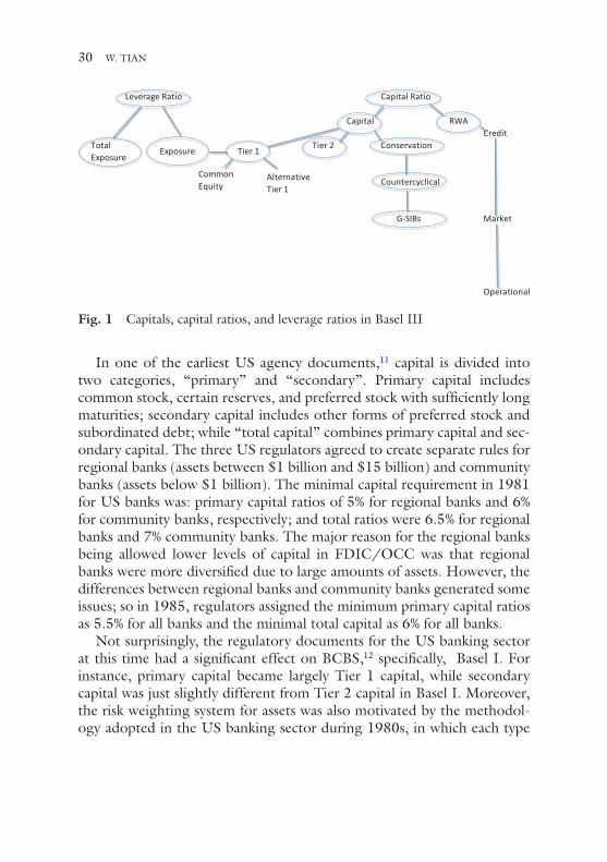
In one of the earliest US agency documents,11 capital is divided into two categories, “primary” and “secondary”. Primary capital includes common stock, certain reserves, and preferred stock with sufficiently long maturities; secondary capital includes other forms of preferred stock and subordinated debt; while “total capital” combines primary capital and sec-ondary capital. The three US regulators agreed to create separate rules for regional banks (assets between $1 billion and $15 billion) and community banks (assets below $1 billion). The minimal capital requirement in 1981 for US banks was: primary capital ratios of 5% for regional banks and 6% for community banks, respectively; and total ratios were 6.5% for regional banks and 7% community banks. The major reason for the regional banks being allowed lower levels of capital in FDIC/OCC was that regional banks were more diversified due to large amounts of assets. However, the differences between regional banks and community banks generated some issues; so in 1985, regulators assigned the minimum primary capital ratios as 5.5% for all banks and the minimal total capital as 6% for all banks.

Not surprisingly, the regulatory documents for the US banking sector at this time had a significant effect on BCBS,12 specifically, Basel I. For instance, primary capital became largely Tier 1 capital, while secondary capital was just slightly different from Tier 2 capital in Basel I. Moreover, the risk weighting system for assets was also motivated by the methodol-ogy adopted in the US banking sector during 1980s, in which each type

Leverage Ratio Capital Ratio

Capital RWACredit

Total Tier 2 ConservationExposure

Common AlternativeEquity Tier 1

Countercyclical

Market

Operational

Exposure

G-SIBs

Tier 1

Fig. 1 Capitals, capital ratios, and leverage ratios in Basel III

30 W. TIAN

of asset had been assigned a different weight—0, 0.2, 0.5, and 1—with the safest assets receiving the lowest number and the riskiest assets receiv-ing the highest number. As has been explained in this chapter, Basel II and Basel III have improved significantly on the risks since the inception of Basel I.

conclusIons

While adequate capital management has been a crucial risk manage-ment tool for commercial banks, and commercial banks are required to implement the major components proposed by Basel III and other regulatory or law requirements (Fed, OCC, FDIC, Dodd-Frank Act in US, and EBA in Europe), we have good reason to believe that some further revisions will be made along the way before January 2023—the official deadline of Basel III—to reflect concerns raised from practitio-ners and academics.

For example, two fundamental questions, among many things, are still subjects to be debated. First, even though we all agree on the characteriza-tion and significance of capital, how much capital is essentially necessary and what is its optimal level? Some argue that the common equity capital ratios should be very high, say 30–50%; while others suggest that a high capital ratio hurts the social optimum so that the capital ratio should be reasonably low. Second, whether or not some total loss-absorbing capac-ity instruments should be treated as regulatory capitals, and, in particular, whether contingent capital should be treated as Tier 1 capital in comput-ing capital ratios? It is also important to design loss-absorbing instru-ments to be consistent with adequate capital requirement.

Other chapters in this book will address some of the most important practices in current regulatory risk management systems. But there are still many unresolved issues and those discussions are beyond the scope of this chapter and this book.

notes

1. Between Basel II and Basel III, a so called Basel II ½ also modifies the existing Basel II. For Basel II ½, we refer to BCBS, “Enhancements to the Basel II market framework”, July 2009; and BCBS, “Revision to the Basel II market framework”, July 2009.


2. Economical capital and other risks such as liquidity risk and legal risk are addressed differently. For the second Pillar and the third Pillar, see BCBS, “International Convergence of Capital Measurement and Capital Standards: A Revised Framework—Comprehensive Version”, Part 3 and Part 4, June 2006.

3. For the leverage ratio in Basel III, see BCBS, “Basel III: A global regula-tory framework for more resilient banks and banking system”, June 2011; BCBS, “Basel III leverage ratio framework and disclosure requirement”, January 2014.

4. For the liquidity risk in Basel III framework, see BCBS, “Basel III: The Liquidity Coverage Ratio and Liquidity Risk Monitoring Tools”, Janua ry 2013; BCBS, “Basel III: The Net Stable Funding Ratio”, October 2014.

5. DVP stands for delivery-versus-payment. Non-DVP trading is defined as securities trading where a client’s custodian will have to release payment or deliver securities on behalf of the client before there is certainty that it will receive the counter-value in cash or securities, thus incurring settlement risk. By the same token, PVP stands for payment-versus-payment, and non-PVP represents non-payment-versus-payment.

6. CPSS represents the Committee on Payment and Settlement Systems and IOSCO stands for the Committee of the International Organization of Securities Commissions.

7. See BCBS, “Guidance for national authorities operating the countercycli-cal capital buffer”, December 2010.

8. US regulators strongly favor common equity Tier 1 only but some European jurisdictions allow high-trigger contingent capital to be used in the capital requirement. For instance, Swiss regulators have already called for the country’s two largest lenders, Credit Suisse Group AG and UBS AG, to issue contingent capitals in addition to meeting a three percentage-point surcharge

9. See FSB, “Reducing the moral hazard posed by systemically important financial institutions”, October 2010; FSB, “Progress and Next Steps Towards Ending ‘Too-Big-To-Fail’ (TBTF)”, September 2013; FSB, “Adequacy of loss-absorbing capacity of global systemically important banks in resolution”, November 2014; and FSB, `“Principles on Loss-absorbing and Recapitalisation Capacity of G-SIBs in Resolution—Total Loss-absorbing Capacity (TLAC) Term Sheet”, November 2015.

10. Its long title is “An Act to prompt the financial stability of the United States by improving accountability and transparency in the financial sys-tem, to end ‘too big to fail’, to protect the American taxpayer by ending

32 W. TIAN

bailouts, to protect consumers from abusive financial services practices, and for other purposes”, effective on July 21, 2010.

11. See “Statement of Policy on Capital Adequacy”, FDIC 1981; “Capital Adequacy Guidelines”, Fed and OCC 1982.

12. For a history of Basel Committee on Banking Supervision (BCBS), see BCBS, “Basel Committee on Banking Supervision (BCBS) Charter”, 2013; BCBS, “A Brief History of Basel Committee”, October 2015; and Adam Lebor, The Shadowy History on the Secret Bank That Runs the World- Tower of Basel, 2013.

references

1. BCBS, “International Convergence of Capital Measurement and Capital Standards”, July 1988. Basel I (the Basel Capital Accord).

2. BCBS, “Basel II: International Convergence of Capital Measurement and Capital Standards: a Revised Framework”, June 2004.

3. BCBS, “Basel II: International Convergence of Capital Measurement and Capital Standards: a Revised Framework – Comprehensive Version”, June 2006.

4. BCBS, “Enhancements to the Basel II Market Framework”, July 2009. 5. BCBS, “Revision to the Basel II Market Framework”, July 2009. 6. BCBS, “Proposal to Ensure the Loss Absorbency of Regulatory Capital at the

Point of Non-Viability”, August 2010. 7. BCBS, “Guidance for National Authorities Operating the Countercyclical

Capital Buffer”, December 2010. 8. BCBS, “Basel III: A Global Regulatory Framework for More Resilient Banks

and Banks System”, December 2010, (rev June 2011). 9. BCBS, “Basel III: International Framework for Liquidity Risk Measurement,

Standards and Monitoring”, December 2010. 10. BCBS, “Basel Committee on Banking Supervision (BCBS) Charter”, 2013. 11. BCBS, “Basel III: The Liquidity Coverage Ratio and Liquidity Risk Monitoring

Tools”, January 2013. 12. BCBS, “Global Systemically Important Banks: Updated Assessment

Methodology and the Higher Loss Absorbency Requirement”, July 2013. 13. BCBS, “Basel III Leverage Ratio Framework and Disclosure Requirement”,

January 2014. 14. BCBS, “Basel III: The Net Stable Funding Ratio”, October 2014. 15. BCBS, “A Brief History of Basel Committee”, October 2015. 16. FSB, “Reducing the Moral Hazard Posed by Systemically Important Financial

Institutions”, October 2010.


17. FSB, “Progress and Next Steps Towards Ending “Too-Big-To-Fail” (TBTF)”, September 2013.

18. FSB, “Adequacy of Loss-Absorbing Capacity of Global Systemically Important Banks in Resolution”, November 2014.

19. FSB, “Principles on Loss-Absorbing and Recapitalisation Capacity of G-SIBs in Resolution – Total Loss-Absorbing Capacity (TLAC) Term Sheet”, November 2015.

20. Lebor, Adam, “The Shadowy History on the Secret Bank that Runs the World”, PublicAffairs, New York, 2013.

34 W. TIAN


Market Risk Modeling Framework Under Basel

Han Zhang

H. Zhang () Wells Fargo & Co. , San Francisco , CA , USA

The view expressed in chapter represents only the personal opinion of author and not those of Wells Fargo & Co.

INTRODUCTION Market Risk is the risk that the value of the bank’s trading portfolio can decrease due to moves in market factors such as equity prices, interest rates, credit spreads, foreign-exchange rates, commodity prices, and other indicators whose values are set in a public market. The risk of losses in both on and off balance sheet positions come from market risk factors’ movement in fi nancial instruments. From the regulatory perspective, the market risk should be managed by the regulatory capital to reduce the market risk of each bank and the bankers’ risk-taking incentive; and thus stabilize the banking sector as a whole. By contrast, individual banks also implement the economical capital for their portfolios.

Since the fi nancial crisis of 2007–2008, market risk management has become more important than ever. Many advanced risk measures and capital charge for market risk are proposed in a comprehensive capital framework.

Given its key position in the regulatory framework, largely on BCBS, this chapter focuses on the market risk modeling framework under Basel. It starts with Basel II to set the major framework of the market risk man-agement. Then it explains its revision Basel 2.5 and highlights its key main points, illustrating several crucial components. Next, two widely used risk measures and their pros and cons are briefl y explained. Finally, the latest revised minimum capital requirement for market risk published in January 2016 is examined.

Introduction to Basel

The Basel Committee on Banking Supervision (BCBS) is a committee of banking supervisory authorities that was established by the central bank governors of the Group of Ten countries in 1974. It is the pri-mary global standard-setter for the prudential regulation of banks and provides a forum for cooperation on banking supervisory matters. Its mandate is to strengthen the regulation, supervision, and practices of banks worldwide with the purpose of enhancing fi nancial stability. The committee is called Basel since the BCBS maintains its secretariat at the Bank for International Settlements in Basel, Switzerland and the com-mittee normally meets there.

BCBS issues Basel Accords (recommendations on banking regula-tions). Three Basel Accords are in existence today – Basel I (1988), Basel II (2007), and Basel III (2010–11).

Basel Accord for Market Risk

In 1988, the Basel Committee published a set of minimal capital require-ments for banks (see [1]). These capital requirements were adopted by the G10 countries, and have come to be known as the 1988 Accord (or Basel I). The general purpose of 1988 Accord was to:

1. Strengthen the stability of international banking system. 2. Set up a fair and consistent international banking system in order to

decrease competitive inequality among international banks.

The 1988 Accord was primarily focused on credit risk and appropriate risk-weighting of assets. Even though market risk was introduced there,

36 H. ZHANG

the 1988 Accord did not require banks to set aside any capital to cover potential losses from market risk. The BCBS was well aware of this issue and saw the 1988 Accord as the fi rst step to establishing a more compre-hensive regulatory capital framework.

Basel I Amendment of 1996

In 1996, BCBS published an amendment to the 1988 Accord to provide an explicit capital cushion for the price risks to which banks are exposed, particularly those arising from their trading activities (see [2]). The amend-ment was originally released in January 1996 and modifi ed in September 1997; it was brought into effect in 1998.

The amendment introduced two main items which had major impacts over many years to the banks’ market risk modeling framework:

1. The accord suggested a general market risk and specifi c risk frame-work. The general market risk refers to changes in market values due to general market movements. Specifi c risk refers to changes in the value of an individual asset due to factors related to the issuer of the security, which is not refl ected in general market movements.

2. Market risk can be calculated in two different ways: either with the standardized Basel model or with internal value-at-risk (VaR) mod-els of the banks. These internal models can only be used by the larg-est banks that satisfy qualitative and quantitative standards imposed by the Basel agreement.

Salient modeling features of the in 1996 amendment about VaR include:

1. Banks using proprietary models must compute VaR daily, using 99th percentile, one-tailed confi dence interval with a time horizon of ten trading days using a historical observation period of at least one year.

2. The capital charge for a bank that uses a proprietary model will be the higher of the previous day’s VaR and a multiplication factor (at an absolute minimum of 3, with a ‘plus factor’ from 0 to 1) times the average of the daily VaR of the preceding 60 business days.

3. Use of ‘backtesting’ (ex-post comparisons between model results and actual performance) to arrive at the ‘plus factor’ that is added to the multiplication factor of three.

MARKET RISK MODELING FRAMEWORK UNDER BASEL 37

The 1997 revision contains the following major changes:

1. The committee decided to remove the provision of the 1996 Market Risk Amendment which requires that the specifi c risk capital charge of the internal models approach be subject to an overall fl oor equal to 50% of the specifi c risk amount calculated under the standardized approach.

2. The committee established certain qualitative and quantitative requirements for idiosyncratic risk which will allow banks that meet them to base their specifi c risk capital charge on modeled estimates of specifi c risk without reference to the fl oor.

3. Introduction of a specifi c risk surcharge aiming at event and default risks.

With the issuing of this amendment, banks fi rst won permission to use internal models to meet the BCBS capital requirement. From 1998, VaR has become established as the industry and regulatory standard in measuring market risk, although the internal model approach in general leads to lower capital charge compared to the prior method of applying fi xed risk weights to different asset classes. BCBS accepted this approach with the view that the models can refl ect the benefi ts of risk diversifi cation strategies and provide incentives for fi rms to develop and implement sound risk management tools.

1996 also marked the time at which regulators, banks’ management and risk management practice began to be more infl uenced by quantita-tive risk modeling, and a new profession of risk quant was in the making.

Basel II

Basel II was revised in between June 2004 and June 2006 (see [3]-[5]), with following major updates:

1. Enhanced risk coverage

a. credit risk b. market risk c. operational risk.

2. A suite of approaches, including standardized- to internal model- based with increasing complexity.

38 H. ZHANG

3. A three pillar approach,

a. the fi rst pillar: minimum capital requirements b. the second pillar: supervisory review c. the third pillar: market discipline.

Basel II of 2004 copied and pasted the capital charge for market risk of the Basel I amendment of 1996.

THE MARKET RISK CAPITAL CHARGE IN BASEL 2.5 FRAMEWORK

After 1996, the fi nancial environments across the globe evolved, with newer fi nancial institutions and more innovative products. The capital charge framework for market risk did not keep pace with these new devel-opment and practices—capital charge for market risk in trading book cali-brated lower compared to banking book treatment on the assumption that markets can provide liquidity for these products, so banks can unwind or hedge these positions quickly. This proved problematic before and during the fi nancial crisis of 2007–2008.

Basel 2.5 Framework

While BCBS realized that a more comprehensive overhaul of the Basel II market risk framework was needed, in the interim it released the so- called Basel 2.5 framework in July 2009 to address the growing concerns over banks’ capital requirement, particularly with the riskier credit-related prod-ucts in mind ([6]). There the several key components in Basel 2.5 framework:

• It supplements the value-at-risk-based trading book framework with an incremental risk capital charge, which includes default risk as well as migration risk, for unsecuritized credit products.

• For securitized products, the capital charges of the banking book will apply with a limited exception for certain so-called correlation trad-ing activities, where banks may be allowed by their supervisor to cal-culate a comprehensive risk capital charge subject to strict qualitative minimum requirements as well as stress testing requirements. These measures will reduce the incentive for regulatory arbitrage between the banking and trading books.


• Introduction of a stressed value-at-risk requirement. Losses in most banks’ trading books during the fi nancial crisis have been signifi cantly higher than the minimum capital requirements under the former Pillar 1 market risk rules. The committee therefore requires banks to calculate a stressed value-at-risk taking into account a one- year observation period relating to signifi cant losses, which must be calculated in addition to the value-at-risk based on the most recent one-year observation period. The additional stressed value-at-risk requirement will also help reduce the procyclicality of the minimum capital requirements for market risk.

In the later adapted US rules, banks were asked to implement Basel 2.5 by January 2013; for banks that have prior approved specifi c risk mod-els, the approval was extended by one year and specifi c risk models were reviewed by US regulators in 2013.

Basel 2.5 is used to as a tactic solution to boost regulators’ confi dence in the capital framework, among all the various changes. Here are a couple of noticeable changes/additions:

Noticeable Changes in the Internal Model Approach Under Basel 2.5

BCBS tightened the qualitative and quantitative criteria in the Basel 2.5 market risk framework. The qualitative and quantitative criteria include the following crucial factors:

• Risk factors

– Factors deemed relevant in pricing function should be included in VaR model (otherwise justifi cation to supervisor)

– Non-linearities for options and other relevant products (e.g. mortgage-backed securities, tranched exposures, or nth-to-default credit derivatives)

– Correlation risk – Basis risk (e.g. between credit default swaps and bonds) – Proxies used should show a good track record for the actual posi-

tion held (i.e. an equity index for a position in an individual stock).

• Scaling methodology (e.g. square-root of time) for the holding period (one day to ten days) is allowed but must be justifi ed periodi-cally to the supervisors.

40 H. ZHANG

• Use of weighting schemes is more fl exible as long as the resulting capital requirements are not reduced.

• Update of data sets should be made, at least on a monthly basis (pro-cess allows more frequent updates).

• Hypothetical (or clean) backtesting is made mandatory for validation. • Stress testing (use of more recent examples for Stress testing

scenarios). • All material components of price risk must be captured. • Surcharge models are no longer allowed.

Noticeable Additions in the Internal Model Approach Under Basel 2.5

There are three newly added models, the incremental risk charge (IRC), the comprehensive risk measure (CRM) and Stressed VaR (SVaR). Although these models do boost the capital requirement, given that the framework requests the total capital charge is the sum of these newly added risk mea-sures with VaR measure, we should notice that some extent of double counting does exist, especially for structure products, the VaR, Stressed VaR, and the standardized charge can easily lead to the total capital change to be more than the 100% of exposure.

In what follows the major challenges in the risk modeling for these models are discussed.

Stressed VaR Stressed VaR is a new measure added in the Basel 2.5 framework; it is designed with the purpose to capital the possible risk under stressed condi-tions. Here are several features of the stressed VaR:

• The current VaR methodology should be used for stressed VaR cal-culation. The intention is to replicate the VaR calculation that would be generated on the bank’s current portfolio if the relevant market risk drivers were experiencing a period of stress:

– Applied to all positions covered under VaR, with consistent meth-odology of 99% and a ten-day horizon,

– The back history is calibrated to historical continuous 12-month period of signifi cant fi nancial stress,

– Since stressed VaR is product or Line of Business (LOB) specifi c, dif-ferent roll-ups may request different stress periods and calibrations.


• An algorithm to search through the history for the continuous 12-month historical period, that stress period should be updated periodically and pre-approved by supervisors.

The fi rst challenging part of stressed VaR modeling is the calibration methodology, a pre-defi ned time range has to be picked up before the search algorithm is started; most banks used data after 2007 to search the stressed period, but were asked to make sure the time period before 2007 did not create a signifi cant loss to the banks’ portfolios.

Although stated in the rule that the GVaR methodology should be used for the stressed VaR calculation, there are two possible deviations in practice by design, because the stressed VaR and GVaR use historical data from two different time periods.

• the historical market data availability can be different for these two periods, and the stress period in general will have less data availabil-ity, caused by less liquidity in the market conditions, or new prod-ucts invented after the stress period. Even where data is available, to retrieve and prepare data going back to, for example, 2007 is a much bigger task compared to dealing with data for just the last two or four years,

• the historical market data shifts in the stressed period are in general larger than the shifts from the regular retrospective period, which potentially can pose a challenge to the bank’s risk P&L estimation method, especially if the fi nancial institution is still using delta- gamma approximation.

But overall, stressed VaR has already started to post more and more challenges into the data modeling given the stressed period resultant from 2008 is aging every day.

Incremental Risk Charge and Comprehensive Risk Measure Two other major models added are the incremental risk charge (IRC) and comprehensive risk measure (CRM). These two models set higher stan-dards on the modeling for default risk, and the risk calculation for correla-tion trading. Following are the highlights of the changes:

• IRC is used to capture credit default risk, which has previously been covered by specifi c risk (SR) models

42 H. ZHANG

– Regulators retrieved banks’ prior approvals of structure products and correlation trading for the debt specifi c risk (DSR) model; under the Basel 2.5 framework, structure products are put into the standardized model and the correlation trading needs to be modeled either in the standardized model or in the newly devel-oped CRM model,

– Event risk is added to the SR model, and default risk is not cap-tured in the SR model anymore, but instead will be captured in the IRC model; the exception is equity products (excluding con-vertibles), which are still included in the equity specifi c risk model for default risk.

• In the IRC model, the default risk is calculated for a one-year time horizon, changed from the ten-day one in the SR model under the old rules. The quantile is also pushed further into the tail from 99%to 99.9%, with a constant level of risk defi nition; these changes dra-matically increased the capital charges for credit default risks.

• The newly developed CRM model captures all risks for correlation trading (synthetic CDO, FTD, and NTD), and the standardized model set a fl oor equivalent to 8% of standard charge, and CRM itself has been proved to be a very diffi cult thing to model.

Risk Not in VaR

Risk not in VaR (RNiV) is an inventory, challenge, and capital overlay program that addresses identifi ed risks which are either not refl ected in the VaR models or modeled with limitations. The program estab-lishes a consistent process for market risk model overlays and for con-trols around these model overlays. RNiV is not written into the Basel 2.5 rules, but it became an integrated part of the framework during the Basel 2.5 model exams, and most of banks got an Matter Requiring Attention (MRA) back in 2012 to build a program to cover RNiV, and later on it also spread into Comprehensive Capital Analysis and Review (CCAR) and Dodd-Frank Act Stress Test (DFAST) programs and also into other modeling areas, and in the more general terms of risk not in model (RNiM).

While models are useful, they do have limitations or even fl aws, the RNiV program gives both model developers and model validators a new


tool to manage these model limitations and fl aws more effi ciently, and also to increase the transparency in these defi cits for model stakeholders, including regulators. In the context of VaR, although the entire gen-eral VaR framework can be approved, the quality of risk modeling varies among different products depend on the following:

• the front offi ce pricing model which the VaR is built on has different qualities;

• the historical market data availability and qualities for different prod-ucts or even trades are different;

• the risk pricing methodology.

For equity trades, credit trades or structure credit trades, regulatory agencies can disapprove products with risk modeling limitations into the IRC/SR standardized charge framework, for conservative capital treat-ment. For rates products, commodity trades or FX trades, the newly cre-ated RNiV framework will give regulator agencies additional capital buffer for modeling limitations.

In general, an RNiV framework should be able to:

• identify, assess, and inventory model limitations, • challenge the RNiV inventory, • provide a quantitative assessment to the inventories’ model

limitations, • establish thresholds to assess the materiality of the quantitative

impacts, • escalate the RNiV inventory to the management, • propose capital overlay for material RNiV items, • propose mitigation plans for RNiV items.

As part of the Basel 2.5 market risk MRA of most of banks, the follow-ing items are very often mentioned:

• including skew risks in VaR • including dividend risks in VaR • including short rate volatilities risk for callable bonds in VaR • including pre-payment and default risks for structure products in

VaR.

44 H. ZHANG

VALUE AT RISK (VAR) AND EXPECTED SHORTFALL (ES) While VaR was widely accepted for market risk capital calculation since 1996, the criticism of its shortcomings never stopped, especially after the fi nancial crisis of 2007–2008, and also with the loss announced by JPMorgan Chase in May 2012.

Value at Risk

Value-at-risk is a measure of potential loss level for a given investment portfolio estimated with a certain confi dence level in a certain period of time, it basically answers the question that how bad things can get. If a bank’s ten-day 99% VaR is $3 million, it means that in ten days, there is a 1% chance that bank’s losses could exceed $3 million.

For the development of VaR methodology, two things are worth noting,

• The underlying mathematics for VaR were developed by Harry Markowitz ([7]) and others in the context of portfolio theory, with the effort to optimize reward for a given level of risk. This happened in 1952, long before the term ‘value-at-risk’ was widely used in the mid-1990s.

• JPMorgan and RiskMetrics: RiskMetrics was launched in 1994, and the technical document outlining the methodology was released in October 1994. JPMorgan and Reuters teamed up in 1996 to enhance the methodology and make data widely avail-able for practitioners and the general public. The effort created a benchmark for measuring market risk and synchronized the meth-odology to calculate it.

The RiskMetrics methodology for calculating VaR assumes that a port-folio or investment's returns follow a normal distribution. RiskMetrics describes three ways to model VaR:

• covariance approach, • historical simulation, which is now a widely used method, • and Monte Carlo simulation.


The Limitations of VaR

VaR is helpful to measure the possible losses, but improper usage of this measure and sometimes focusing too narrowly on this one measure alone can lead to serious mistakes. Among the major issues are the following:

1. VaR provides a point measure at pre-defi ned quantile. It provides no information about the maximum losses that could happen. In another words, VaR can tell you that by 1% chance a portfolio can lose $3 million, but not the information that there is for example a 0.01% chance the portfolio can lose $3 billion or even more.

2. VaR is not a coherent measure. A coherent risk measure is a risk measure defi ned to satisfy a set of properties. In particular, there is one property named subadditivity, means the risk of two portfolios together cannot get any worse than adding the two risks separately; this is the diversifi cation principle. An unrecognized violation of subadditivity property can lead to serious consequences for risk models, like providing a false sense of security or leading a fi nancial institution to make a suboptimal investment.

3. VaR assumes normal market conditions and that a trade can be easily liquidated; it can give false information under stressed conditions or when market liquidity has dried up.

4. VaR projects are based on historical observations, where the histori-cal period looked back to may not be able to cover all the possible future outcomes. VaR is also limited in capturing credit risk, discrete event risks, and structural shifts in the economy.

Expected Shortfall

Just two years after VaR was adapted by Basel in the capital calculation, academic researchers in 1998 began to criticize that VaR has fundamen-tal structure fl aws, and said it should be replaced by coherent risk mea-sures. In 2001, expected shortfall (ES) was adapted worldwide to be used side- by- side with VaR. For the next fi fteen years, there were many academic debates about whether VaR should be replaced by expected shortfall .

Expected shortfall is also called conditional VaR or tail loss; it is a coher-ent risk measure. ES estimates the expected return on a portfolio of the loss tail, thus it is more sensitive to the shape of the loss distribution in the tail. Since ES provides average loss in a worst case scenario, it can be

46 H. ZHANG

very sensitive to extreme “outliers”. Therefore, more observations than VaR at the same confi dence level may be needed in order to have the same accuracy. A heavy tail in the loss distribution also indicates a big difference between VaR and ES.

THE MINIMUM CAPITAL REQUIREMENTS FOR MARKET RISK In January 2016, BCBS published the new Minimum Capital Requirements for Market Risk (also called FRTB). See [8]. This is the latest Basel ini-tiative to overhaul the Basel 2.5 framework with a more coherent and consistent framework. While Basel 2.5 was implemented in the immedi-ate aftermath of the fi nancial crisis as a stop-gap measure to lift trading book capital requirements, the Fundamental Review of the Trading Book (FRTB) is primarily aimed at consolidating existing measures and reduc-ing variability in capital levels across banks.

Consistent with the policy rationales underpinning the committee’s three consultative papers on the Fundamental Review of the Trading Book (see [9]-[11]), the revised market risk framework consists of the following key enhancements.

A Revised Internal Models Approach (IMA)

The new approach introduces a more rigorous model approval process that enables supervisors to remove internal modelling permission for individual trading desks, more consistent identifi cation and capitalization of material risk factors across banks, and constraints on the capital-reducing effects of hedging and diversifi cation.

The new proposed P&L attribution test, as part of the model approval process, will go forward as a main focus for banks and risk quants. The new approval process will be desk by desk, with much more scrutiny on risk calculation for individual products. By doing P&L attribution tests, risk quants have to develop tools to test following items:

• identify missing risk drivers, • fi gure out defi ciency of the risk P&L calculation method, • improve the data modeling in the risk modeling.

This effort will also promote the alignment between the risk views with the trading views on risk, and give regulators more insights into the


trading business while they are reviewing the risk models; at the same time this also will promote higher standards at front offi ce in their pricing and data modeling practice.

The next thing worth mentioning in the new IMA is the modellable and non-modellable risk factor; it formalizes an approach when a risk factor can-not be properly modelled in the IMA. As a general practice in the current RNiV process, a stress scenario-based approach is widely used for RNiV quantitative estimation; the new rule asked that “Each non- modellable risk factor is to be capitalized using a stress scenario that is calibrated to be at least as prudent as the expected shortfall calibration used for modelled risks.” This can formally move most items in the RNiV inventory into the modeling framework with a workable guideline on the practice.

The new framework also reduces the benefi t of the diversifi cation and hedge effect in the IMA approach across the asset classes, but the impact still needs to be checked in the future.

A Revised Standardized Approach (SA)

The revisions fundamentally overhaul the standardized approach to make it suffi ciently risk-sensitive to serve as a credible fallback for, as well as a fl oor to, the IMA, while still providing an appropriate standard for banks that do not require a sophisticated treatment for market risk.

In the Basel 2.5 framework, a standardized model covers credit prod-ucts, equity products and credit structure products. In the new framework, in order to serve as a credible fallback option for IMA, the standardized approach is extended to cover all products. In the fi rst consulting paper, two approaches were proposed by BCBS, and the sensitive based approach got overwhelming acceptance over the cash fl ow-based approach.

The newly proposed standardized approach is dramatically different from the old factor-based approach; it is a parametric VaR-like approach with pre-defi ned parameters from regulators, and a very detailed pre-scribed approach. There are many industry discussions on how the new rules can fi t to all different products, and try to understand how to apply rules from the text and spirit of the rule.

Although BCBS mentions that a standardized approach can serve as a fl oor to the IMA approach, the rule itself does not specify how the fl ooring mechanism should work, and it requests fi nancial institutions to calculate the standardized approach no matter if there is an approved IMA approach or not. Since the banks are still waiting for the nationalized rule,

48 H. ZHANG

such a fl ooring mechanism can be refl ected there; otherwise it will be subjected to the local regulators when they approve the IMA approach for each fi nancial institution.

Overall, the standardized approach can lead to higher capital for some products; especially products in the old framework only can have IMA approach. But for structure products which can have multiple charges from VaR, stressed VaR, and standardized charge, the new standardized approach as a single measure will not likely lead capital charge to be more than 100% of exposure, thus it may lead to less capital compared to cur-rent Basel 2.5 treatment.

A Shift from Value-at-Risk to an Expected Shortfall Measure of Risk Under Stress

Use of ES will help to ensure a more prudent capture of ‘tail risk’ and capital adequacy during periods of signifi cant fi nancial market stress.

As discussed in the previous section and also stated by BCBS, ES cap-tures more information on the loss tail. As for implementation, if a bank has a good simulation model, VaR and ES are just two different risk mea-sure outputs, and the implementation challenge is virtually small.

Along with the ES, BCBS also introduced full set/reduce set concept to combine VaR and stressed VaR risk measures. The full set/reduce set methodology is trying to fi x the data availability issue mentioned in the Basel 2.5 stressed VaR modeling. Although there were many discussions in the Basel 2.5 model approval process regarding that if a bank can proxy data using the statistics from the normal time period for the stressed look- back period, it seems there is an agreement and BCBS took the approach to assume the ratio of ES between a full set with a reduced set of risk driv-ers to be the same between the stressed period and normal period—or at least this is the best approach without more information.

Another thing about ES is the backtesting. As Gneiting and others have pointed out, elicitability is a desirable property when it comes to “making and evaluating point forecasts”, but since ES does not possess this mathematical property, thus it could not be backtested ([12]). Acerbi and Szekely proposed three model-independent, non-parametric backtest-ing methodologies (see [13]). In the new framework, the backtesting is still fall back to a one-day VaR risk measure, with the assumption that the underlying methods used are the same between VaR and ES.


Incorporation of the Risk of Market Illiquidity

Varying liquidity horizons are incorporated into the revised SA and IMA to mitigate the risk of a sudden and severe impairment of market liquidity across asset markets. These replace the static 10-day horizon assumed for all traded instruments under VaR in the current framework.

Capital is now calculated to a longer time horizon of up to one year dependent on the types of risk drivers, which does have the impact that the risk is calculated more segmentally to risk drivers instead of to individual trades, and makes the models defi ned in the new framework more prudent regarding capital calculation, but less transparent for risk management purposes. As defi ned by BCBS in the new framework, risk management may use different methodology/models, pending regulatory approval.

A Revised Boundary Between the Trading Book and Banking Book

Establishment of a more objective boundary will serve to reduce incentives to arbitrage between the regulatory banking and trading books, while still being aligned with banks' risk management practices.

The new regulation is stricter, to prevent fi nancial institutions from moving assets between regulatory banking and trading books, while risk has to team up with fi nance and FO on a regular basis to discuss the boundary between the trading book and banking book. It is also not clear yet how fi nancial institutions will take care of the regulatory desks com-pared to the Volcker desks.

CONCLUSION As can be seen from recent history, regulations and capital calculation methodology did evolve with the fi nancial crisis, and as a result, the indus-try would also be reshaped by the new regulations. After the publishing of the new regulations in January 2016, the fi nancial industry and regulators still need time to set down the new Minimum Capital Requirements for Market Risk; we do believe the new rules in general provide better regu-lation compared to Basel 2.5, and they have addressed several structural issues observed in the last couple of years. As for the impacts of the new rules to the fi nancial industry, there are theories, but the real impact will still need to be seen in the coming years.

50 H. ZHANG

NOTES 1. BCBS, “International Convergence of Capital Measurement and Capital

Standards”, July 1988. Basel I (the Basel Capital Accord). 2. BCBS, “Amendment to the Capital Accord to Incorporate Market Risks”,

January 1996 (Amendment). See http://www.bis.org/publ/bcbs24.htm . 3. BCBS, “Basel II: International Convergence of Capital Measurement and

Capital Standards: a Revised Framework”, June 2004; BCBS, “Amendment to the Capital Accord to Incorporate Market Risks”, Updated November 2005; BCBS, “Basel II: International Convergence of Capital Measurement and Capital Standards: a Revised Framework – Comprehensive Version”, June 2006.

4. BCBS, “Revisions to the Basel II market risk framework – fi nal version”, July 2009.

5. Markowitz, Harry, M., Portfolio Selection, Journal of Finance , 7 (1), 77–91, 1952.

6. BCBS, “Minimum Capital Requirements for Market Risk” (Standards), January 2016.

7. T. Gneiting, Making and evaluating point forecasts, Journal of the American Statistical Association , 106(494):746–762, 2011.

8. C. Acerbi and B. Szekey, Backtesting Expected Shortfall , December 2014.

REFERENCES 1. BCBS, “International Convergence of Capital Measurement and Capital

Standards”, July 1988. Basel I (the Basel Capital Accord). 2. BCBS, “Amendment to the Capital Accord to Incorporate Market Risks”,

January 1996 (Amendment). 3. BCBS, “Basel II: International Convergence of Capital Measurement and

Capital Standards: A Revised Framework”, June 2004. 4. BCBS, “Amendment to the Capital Accord to Incorporate Market Risks”,

Updated November 2005. 5. BCBS, “Basel II: International Convergence of Capital Measurement and

Capital Standards: A Revised Framework – Comprehensive Version”, June 2006.

6. BCBS, “Revisions to the Basel II market risk framework - fi nal version”, July 2009.

7. Markowitz, Harry, M., Portfolio Selection, Journal of Finance , 7 (1), 77-91, 1952.

8. BCBS, “Minimum Capital Requirements for Market Risk” (Standards), January 2016.


http://www.bis.org/publ/bcbs24.htm

9. BCBS, “Fundamental Review of the Trading Book”, May 2012. 10. BCBS, “Fundamental Review of the Trading Book: A Revised Market Risk

Framework”, October 2013. 11. BCBS, “Fundamental Review of the Trading Book: Outstanding Issues”,

December 2014. 12. Tilman Gneiting., Marking and Evaluation Point Forecasts, Journal of the

American Statistical Association , 106(494): 746–762, 211. 13. C. Acerbi and B. Szekey, Backtesting Expected Shortfall, December 2014.

52 H. ZHANG

Counterparty Credit Risk


IMM Approach for Managing Counterparty Credit Risk

Demin Zhuang

D. Zhuang (*) Citigroup, 1 Court Square, 35th Floor, Long Island City, NY 11120, USAe-mail: [email protected]

The view expressed in chapter represents only the personal opinion of author and not those of his current and previous employers.

IntroductIon

The counterparty risk of a bank is the risk of economic loss due to the default of its counterparty of either an over-the-counter (OTC) derivative trade or a transaction of securities financing before the final settlement of the transaction's cash flows. A recent striking example is in 2008, when several credit events happened within a one-month time period: at Fannie Mae, Freddie Mac, Lehman Brothers, Washington Mutual, Landsbanki, Glitnir, and Kaupthing. It is apparent that counterparty risk is one of the major drivers of the financial crisis we experienced in 2007–2008. Counterparty credit risk (CCR), which causes economic loss due to coun-terparty default and credit rating downgrade, is an essential part of finan-cial risk management in most financial institutions. It is similar to other forms of credit risk in many aspects, however, a distinct feature of CCR, the uncertainty of exposure of a bank to its counterparties, sets it apart significantly from other forms of credit risk.


When a counterparty defaults, the bank must close out its positions with the defaulting counterparty. To determine the loss arising from the counterparty’s default, it is often assumed that the bank enters into a similar contract with the counterparty in order to maintain its market position. Since the bank’s market position is unchanged after replacing another contract, the loss is then determined by the contract’s replace-ment cost at the time of default. If the contract value is negative for the bank at the time of default, the bank closes out the position by paying the defaulting counterparty the market value of the contract, while entering into a similar contract with other counterparty and receiving the market value of the contract—thus it has a net loss of zero. On the other hand, if the contract value is positive at the time of the counterparty default, then the bank closes out the position with zero recovery, enters into a similar contract with other counterparty but pays market value of the contract. In this case, the net loss of the bank is non-zero and is in fact the market value of the contract.

Notice that plausible replacement of the contract implies that there is an adequate liquidity of the contract in the market. However, loans rarely have a liquid secondary market. It is difficult to determine the replace-ment cost of a contract. For this reason, counterparty risk of these types of transactions is not addressed in this chapter.

In order to manage counterparty credit risk, Basel II and III set out specific requirements for risk capital calculation related to OTC and secu-rities financing transactions (SFT) such as asset loans and repo, and reverse repo agreements, with exposures implied by the potential one-year hori-zon counterparty default. Standard approach (SA) and internal model methods (IMM) are two different approaches for measuring counterparty credit risk subject to the approvals from regulators. This chapter focuses on the IMM approach.

MotIvatIons of developIng IMMInternal model methods encourage the bank to build a set of consistent pricing and analytics environments across front and back offices so that estimating exposures of portfolios will be more accurate, with full net-ting benefits. Netting occurs based on a legal netting agreement in place between the parties (“ISDA”). Consequently, the implementation of IMM usually results in significant capital saving, once the implementation is approved by regulators.

56 D. ZHUANG

In order to quantify the counterparty credit risk using the IMM approach, a bank builds a counterparty credit risk management infrastruc-ture which is the centralized analytic engine that provides on-demand cal-culation of credit exposure at counterparty level, supporting netting and margining agreements. The analytic engine can estimate the distribution of potential replacement cost, or exposure to price movement through liquidation in OTC derivative trading and securities finance transactions (SFT). The main component of the engine is the Monte Carlo simula-tion process. The process simulates the behaviors of the underlying mar-ket factors (also known as risk factors) related to these trades at future dates based on their assumed dynamics of evolution and on the covariance structures and volatilities estimated from historical time series. The ana-lytic engine also has functionalities for aggregating the exposures at given levels and generating the appropriate reports.

In general, a financial institution often has a portfolio of multiple trans-actions with each one of its counterparties. Thus, the exposure of the bank to the counterparty is the sum of the replacement costs of all the positions with a counterparty. The potential credit risk exposure to this counterparty can be calculated over the longest life of the transactions in a portfolio using a Monte Carlo simulation. The bilateral nature of coun-terparty credit risk means that the netting agreements of the bank and its counterparties must be taken into consideration when estimating the counterparty credit risk. The full simulation of all relevant market factors together with contractual netting and margining agreements allows an accurate and consistent capturing of portfolio effects. Each transaction in the portfolio is revalued using simulation paths at discrete intervals: The mark-to-market values of the portfolio under these simulated scenarios at each of future time point are obtained. The distributions of simulated mark-to-market prices are then calculated at specified confidence levels. Regulatory required expected positive exposure (EPE), potential future exposure (PFE), and other quantities for quantifying counterparty expo-sure are computed based on these distributions.

Several points are worth mentioning at this stage. First, for most market factors, the dynamics of evolution of market factors are assumed to follow lognormal distributions. The assumption is an industrial standard and has been commonly used by financial industry practitioners and is supported by academic researchers and by empirical evidence. On the other hand, different dynamics are also used to simulate market factor evaluations. Financial institutions are free to choose simulation dynamics, as long as

IMM APPROACH FOR MANAGING COUNTERPARTY CREDIT RISK 57

they are able to demonstrate to regulators that such chosen simulation models are conceptually sound, robust, and stable using sensitivity analy-sis, stress testing, and backtesting results.

Second, another important assumption, not necessarily consistent with market reality, is that the portfolio remains constant within the simulation process. In other words, no transactions take place for the entire life of the portfolio. The implication of the assumption is that the exposure estima-tion process is required to run frequently, usually on a daily basis, with updated market factor values and updated portfolio structures.

Third, the covariance structures and volatilities used in the Monte Carlo simulation process are calibrated to historical Profit and Loss (P&L) movements. The covariance structures and volatilities remain constant during the entire simulation period. This is clearly a simplification of market reality. Consequently, the covariance structures and volatilities are required to be updated on a regular basis to reflect current market conditions. Actually, regulators have started to request financial firms to consider dynamic volatilities and even dynamic covariance matrices for the progress of simulating counterparty risk exposure.

Last but not the least, there are other means of mitigating counterparty credit risk in OTC trading. For example, collateral agreements which reduce the exposure by the amount of collateral held as of the last rebal-ancing; CVA calculation and using of a central clearing house, and so forth Collateral method and CVA methods are addressed in other chapters of the book (Chap. 4).

Monte carlo sIMulatIon fraMework

Briefly, a Monte Carlo simulation framework using covariance matrices and volatility structures calibrated to historical price movements emulates the behavior of the underlying market factors relevant to the trades in the portfolio at future dates. The full simulation of these market factors together with different netting and margining rules allows an accurate and consistent capturing of portfolio effects. Each transaction in the portfolio is revalued using all generated simulation paths at discrete intervals. The mark-to-market values of the portfolio under these simulated scenarios at each of time periods are obtained. The distribution of simulated mark-to- market prices is then calculated at a specified confidence level.

In the following, we present details of the Monte Carlo simulation framework summarized above.

58 D. ZHUANG

http://dx.doi.org/10.1057/978-1-137-59442-6_3

There are several main components in an analytic engine for calculating the distribution of counterparty-level credit exposure.

Market Factor Simulation

In order to estimate the credit exposure to the counterparty, we first gen-erate potential market scenarios at a fixed set of simulation dates in the future. Market scenarios consist of realization of a set of market factors relevant to all the trades with the counterparty at specified future dates. These market factors are of two categories: those that are simulated and those are not and remain static along each path into the future. For exam-ple, historical volatility and correlations of underlying market factors are often assumed to be constant throughout the simulation process whereas interest rates, foreign exchange (FX) rates, and credit spreads are assumed to follow certain dynamics and are simulated at each simulation date in the future. The assumptions of constant volatilities of market factors and of constant correlation structures are mainly for the sake of simplicity of the modeling. These model assumptions are the idealized abstractions of the market reality, albeit being overly simplified abstractions. They are often regarded as the model limitations and might lead to model risk. The corresponding compensating controls consist of frequent updating of the volatility and correlation structures as well as regular model performance monitoring and review.

The scenario generation process consists of a number of simulation models that produce simulation paths of market factors related to the con-tracts in the portfolio. Some common market factors often required for OTC derivatives are the following:

• Interest rates;• Credit spreads;• FX rates;• Stock and index spot prices;• Commodity future prices;• Volatility surfaces;• Correlation skews for CDO tranche trades.

In general, for xi representing one of the market factors above, and if we assume that xi is lognormal distributed then these market factors can be simulated using the dynamic of


dd d

x

xt W ti

ii i i= + ( )µ σ ,

with the property that

d d dW t W t ti j ij( ) ⋅ ( ) = ρ

where the drift μi, volatility σi and correlations ρij are assumed to be constant.

Volatilities and correlation parameters should be periodically updated from historical data.

The simulation dynamics can be different for different market factors. In fact, different financial institutions do use dynamics other than lognormal for market factor simulations.1 The key here is that the IMM model developers should be able to convince regulators of the conceptual soundness, robust-ness, and stability of the model framework for chosen simulation dynamics.

Trade Pricing at Future Scenarios

Next, we consider the value of the portfolio at a future time. For each simulation date and with each realization of the underlying market risk factors, all trades in the portfolio are priced using the pricing libraries of front office for the market scenarios generated by the simulation pro-cess described above. Front office pricing libraries are usually rigorously validated and already approved by the regulators. They can price trades at a very accurate level. Leveraging the front office pricing libraries allows the consistency in trading, market risk management, and counterparty risk management of the firm.

In the past, for a large financial institution, applying front office pric-ing libraries to estimate counterparty credit exposure was difficult due to the intensity and complexity of computation effort involved. Defaults or credit rating transitions of underlying issuers are events with small proba-bilities. Without a sufficient number of simulation paths, these rare events are difficult to be fully captured. Thus, each trade in the portfolio must be evaluated at future date points for many thousands of simulated future scenarios, in addition to applying high degrees of complexity on portfolio netting and margining algorithms.

60 D. ZHUANG

Nowadays, with the available parallel computing grids and ever increasing computation power, integrating simulation processes with the pricing libraries of trading desks has become possible for many products. However, path-dependent trades such as American/Bermudan and asset- settled derivatives present additional challenges for valuation, due to the fact that the values of these trades may depend on either some event that happened at an earlier time (e.g. exercising an option) or on the entire path leading to the valuation date (e.g. barrier or Asian options). Typically, analytical approximations or simplified valuation models will have to be used for these products.

Exposure Profile Generation

For each simulation date and for each realization of the underlying market risk factors, counterparty-level exposure is obtained by applying necessary netting and margining rules.

Future exposure to a counterparty can be visualized by means of expo-sure profiles. These profiles are obtained by calculating certain statistics of the exposure distribution at each simulation date. For example, the expected positive exposure profile (EPE) is obtained by computing the expectation of exposure at each simulation date, while a potential future exposure profile (PFE) is obtained by computing a high-level (e.g. 97.7% or 99%) percentile of exposure at each simulation date. Though profiles obtained from different exposure measures have different magnitudes, they usually have similar shapes.

The following figure outlines the three components, scenario genera-tion, pricing, and aggregation of the framework (Fig. 1).

Implementation of the Components

The implementation of these three components described above is pre-sented as follows:

Let P be the portfolio of trades against a particular counterparty. Assume that P consists of N related trades. These trades are denoted by A1 , A2 , … , AN. For simplicity, I do not take the margining into consid-eration for now. The valuations of these instruments on a discrete set of future simulation dates are performed based on simulated market factors at these future time points. Let t0 be the valuation date (current date) and t1 , t2 , … , tn be the set of dates in the future at which we simulate market


risk factors, where tn is the longest maturity of the trades. More specifi-cally, let Mj be the time period (in units of years) between the valuation day and maturity of trade Aj for j = 1 , 2 , … , N.

Let M be the longest time period defined as

M M j Nj= = …{ }max : , , .1 2,

If the simulation is carried out on a set of equal length time grids, then we can easily determine the number of steps required for the simulation process as follows:

Fig. 1 Three components in counterparty risk management framework

62 D. ZHUANG

Let l be the length of the unit time interval of the simulation. Then the required number of time steps for the simulation process, denoted by n, is given by the following:

n

M

l= +

1 .

The length of time step needs not to be constant throughout the simu-lation process. It makes sense to use more granular time steps in the begin-ning of the simulation, which indicates our confidence in the simulated MTM values. For example, we can have predefined time step granularity as follows:

• Daily step up to a week;• Weekly step up to a month;• Monthly step until the maturity M.

All market factors relevant to the trades in the portfolio P have to be simulated together. With a little care, the number of simulation steps can be calculated for any given portfolio against a counterparty. For the sake of preciseness of our presentation, we assume that there are n time intervals for the entire simulation period, with the understanding that first a few time intervals are of different lengths than the monthly time intervals.

The exposure of the portfolio P against its counterparty at the confi-dence level α is the maximum of the set of values {P(tk) : k = 0, 1, 2, … , n}, where P(tk) is the α-th percentile of the set of portfolio values under the simulated market factor values at a particular future point of time tk.

Suppose that the total number of simulations is S. Let m be used to index the simulated scenarios: m = 1 , 2 , … , S. We calculate the potential market value of each transaction at each future date of each simulated path. Let Am

j (tk) be the potential market value of trade Aj at time tk under the m-th scenario. Let P(m)(tk) be the current exposure of the portfolio at time tk under the m-th scenario.

Then

P t A tmk

j

N

j

m

k( )

=

( )( ) = ( )∑

1

˜

,


where A tj

m

k

˜ ( )( ) is defined as

A tA t

A tj

m

k

jm

k

jm

k

˜

{,

,.

( )( )

( ) +( ) =( )

( )

if nettable

otherwise

Here, we define[x]+ = max {0, x}.The basic simulation algorithm can be described as follows

Step 1 Compute the portfolio’s value at time t0. This value should match the market price of the portfolio. This is checked by “tolerance tests”;

Step 2 Set m = 1;Step 3 Call market factors simulation process to generate values of

relevant market factors over the time interval [t0, t1]Step 4 Compute the value of the portfolio at time t1;Step 5 Repeat Step 3 to Step 4 for time steps t1 , t2 , … , tn to

compute P(1)(t2) , P(1)(t3) , P(1)(t4) , … , P(1)(tn),Step 6 Set m = m + 1. Repeat the scenario simulation process (Step

2 to Step 5) S times to obtain the following P t P t P tm

m

Sm

m

Sm

m

( ) +

=

( ) +

=

( ) +

=( )

{ } ( )

{ } ( )

{ }0

11

12

1

, ,SS

mn

m

S

P t, ,… ( )

{ }( ) +

=1

The α-th percentile of the above sequences, denoted by PFEα(tk), k = 0, 1, 2,..., n, form the PSE profile of the portfolio with the confidence inter-val α. The peak PFE at the confidence level α, denoted by PFEα, is given by the following formula:

PFE PFE t k nkα α= ( ) = …{ }max : , , , ,0 1 2

For example, we can use the percentile level of α = 97.7% or α = 99.0%.We can also compute EPE (expected positive exposure), which is

defined as the maximum of expected positive exposure at each of the time steps t0 t1 , t2 , … , tn. Specifically, at time step t1, we compute

64 D. ZHUANG

EPE t

SP tk

S

mm

k( ) = ∑ ( )

= ( ) +1 1

EPE profile consists of all EPE(tk) for k = 0 , 1 , … , n. The peak EPE of the portfolio P is the maximum of the sequence EPE tk k

n( ){ }=0

.

Calculation of Effective EPE

In July 2005 the BCBS announced a number of significant changes to the revised framework, designed to address the perceived weaknesses. The Basel II framework permits, for the first time, banks to use advanced internal model approaches to calculate regulatory capital, reducing capital requirements by applying techniques long accepted as ‘best practice’ when calculating internal credit risk. At the heart of the new approaches is the accurate calculation of expected exposure (EE) and EPE. Importantly, EE must be computed with the same sophisticated models used to calculate Potential Future Exposures (PFE), by simulating exposures in market sce-narios on various future dates.

Expected exposure at future date t, denoted by EEt, is the average posi-tive exposure at t. In other words, EEt = EPE(t). The effective expected exposure, denoted by effective EE, is computed recursively as

effective effective ,EE EE EEt t tk k

= { }−

max1

The effective EPE is defined as the average effective EE during the first year of future exposure. If all contracts in the netted portfolio mature within less than one year, then effective EE is defined as the average of effective EE until all contracts in the portfolio mature.

We also compute effective EPE as a weighted average of effective EE as follows:

effective effective

,maturityEPE EE

y

k

t kk= ∑ ×

{ }

=

min 1

1

where Δk = tk − tk − 1. Note that the weights Δk allow for the case when future exposure is calculated at dates that are not equally spaced over time.


With these computed quantities, we can calculate the exposure value as the product of alpha (α) and effective EPE.

Exposurevalue effectiveEPE= ×α

where α is set equal to 1.4, according to Basel II revised framework. This parameter adjusts the regulatory capital estimates for:

• The exposures’ volatilities, correlations of exposures across counter-parties, correlation between exposures and defaults, that is wrong- way risk;

• The potential lack of granularity across a firm’s counterparty exposures;

• Model, estimation, and numerical errors.

The Basel II framework allows for the use of a shortcut method, with simple and conservative approximation to the effective EPE instead of applying a life-time simulation method, for netting sets with an accom-panying margin agreement. The effective EPE for a margined counter-party can be calculated as the sum of the threshold plus an add-on that reflects the potential increase in exposure over the margin period of risk, or effective EPE without a margin, whichever is lesser. Under the internal model method, Basel II requirements state that a measure that is more conservative than effective EPE may be used in place of alpha times effec-tive EPE. There is a great deal more that can be said specifically related to margined counterparties. The reader is referred to other chapters of this book for details.

Backtesting Methodology

To use IMM for CCR, a financial institution is required to provide evi-dence to supervisory authorities that the IMM framework is conceptually sound and is implemented with integrity. Regulators specify a number of qualitative criteria that the financial institution must meet. One of the qualitative criteria for CCR exposure model framework is backtesting. The Basel regulatory capital framework requires that IMM banks back-test their expected positive exposure (EPE) models, where backtesting is defined as the quantitative comparison of the IMM model’s forecasts

66 D. ZHUANG

against realized values. Regulators do not prescribe specific methodologies or statistical tests for backtesting.

The backtesting methodology is based on a standard statistical infer-ence approach, in order to make a determination of whether the historical exposure behavior falls into the range of the model prediction. The basic idea of the backtesting methodology is to show that the historical path is not distinguishable from the simulated forecast paths statistically at some confidence level. In other words, the backtesting statistically compares the historical path against simulated paths and evaluates a model’s successful-ness of forecasting the future evolution of observables.

A backtesting process includes the selection of the test data; the selection test portfolios and market; and the selection and develop-ment of appropriate statistical tests, as well as the interpolation of the test results. The backtesting is performed on both market factors and hypothetical portfolios. For backtesting on hypothetical portfolios, the ex-ante exposures predicted by the model (for a percentile or average) over a specific time window (typically one year) form barriers for the backtesting.

We say the test is successful at a given simulation time point if the his-torical portfolio value at this point is less than the barrier. Otherwise, we say there is a break at this point of time. We then count the number of breaks that have occurred over the window. Different statistical properties of the distributions of breaks for multiple portfolios over multiple time windows are studied and tested.

Market factor backtesting covers major market factors such as equity spots, interest rates, credit spreads, commodities, and foreign exchange. Backtesting results reflect the direct simulation model performance of that particular market factor. As an illustration, we perform a backtesting on a market factor with several percentiles: for example 1%, 2.3%, 15%, 35%, 65%, 85%, 97.7%, and 99%, as following Fig. 2 shows:

Hypothetical portfolio backtesting is conducted on both PFT (for a given percentile) and EPE directly. Historical MTM of the portfolio is constructed by pricing each trade using the historical market data (price, rates, and implied volatilities). The following Fig. 3 illustrates a simple example of backtesting. In Fig. 3, a single trade portfolio of a Greek 5 year CDS contract for a protection buyer with $10,000,000 notional is back-tested for test period of September 30, 2010 to September 30, 2011. The underlying credit spreads increased to very high levels during the period.


Backtesting results indicate that PFE (with 97.7%) is sufficiently conserva-tive as there are not breaks for the entire test period. However, EPE does show many breaks and indicates the inadequacy of EPE in a stress period.

As another example, we consider the stress period of December 31, 2010 to—December 31, 2011, remembering that the Euro crisis and US

Fig. 2 Market factors for backtesting

Fig. 3 An example of backtesting

68 D. ZHUANG

rating got downgraded in the summer of 2011. Backtesting results of iTraxx 7 6–9% tranche protection buyer maturing on June 20, 2012 in the following figure, Fig. 4, show that as the credit market began to deterio-rate, a large amount of breaks appeared even for PFE at 97.7% level. In this case, we say the trade failed the backtesting over the test period.

There are different approaches and statistical analyses for IMM models measuring counterparty credit exposure. As backtesting of IMM models for CCR has yet to be solidified into a definitive methodology commonly adopted by industry and regulators, a financial institution has the ability to develop its own backtesting techniques.

a case study

In this section, a simple interest swap is used to illustrate the IMM meth-odologies discussed above. We consider simple 5y interest rate swaps in a single currency. Thus, the only market factor to be simulated is the interest rates. We simulate interest rates by using common simulation models of the term structure of interest rates. Fig. 5 illustrates the simulated interest rates in the future times:

With simulated future market factor values (in this case, interest rates only), we can evaluate the values of the swap at future time grids, as shown in Fig. 6. These are the mark-to-market values of the swap using simulated market factor values.

Fig. 4 Another example of backtesting


Simulated future market factor values

0

0.3

0.2

0.1

0.0

−0.1

−0.2

−0.3

−0.41 2

Time in years

Sim

ula

ted

mar

ket

fact

or

valu

es

3 4 5

Fig. 5 Illustration of simulated interest rates in the future dates

3.0le7

2.0

2.5

1.5

1.0

0.5

0.0

−0.5

−1.0

−1.50 1 2

Time in years

NP

V

3 4 5

Simulated MtM paths

Fig. 6 Prices of the portfolio under the similated scenarios

70 D. ZHUANG

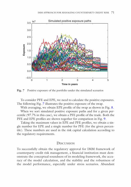
To consider PFE and EPE, we need to calculate the positive exposures. The following Fig. 7 illustrates the positive exposure of the swap.

With averaging, we obtain EPE profile of the swap as shown in Fig. 8.When we sort simulated positive exposure paths and for a given per-

centile (97.7% in this case), we obtain a PFE profile of the trade. Both the PFE and EPE profiles are shown together for comparison in Fig. 9.

Taking the maximum values in EPE and PFE profiles, we obtain a sin-gle number for EPE and a single number for PFE (for the given percen-tile). These numbers are used in the risk capital calculation according to the regulatory requirements.

dIscussIon

To successfully obtain the regulatory approval for IMM framework of counterparty credit risk management, a financial institution must dem-onstrate the conceptual soundness of its modeling framework, the accu-racy of the model calculation, and the stability and the robustness of the model performance, especially under stress scenarios. Abundant

3.0

3.5

2.0

2.5

1.5

1.0

0.5

0.0

−0.5

Exp

osu

re

0 1 2

Time in years

3 4 5

Simulated positive exposure pathsle7

Fig. 7 Positive exposure of the portfolio under the simulated scenarios


Expected Exposure

Exp

ecte

d E

xpo

sure

le71.0

0.8

0.4

0.6

0.0

0.2

0 1 2Time in years

3 4 65

Fig. 8 The expected exposure profile over five years

3.0

le7

2.0

2.5

1.5

1.0

0.5

0.00 1 2

Time in years

Exp

osu

res

3 4 5 6

PFE and EPE together

Fig. 9 EPE and PFE of 97.7 percentile

72 D. ZHUANG

evidence, such as results of backtesting and sensitivity analysis of the framework, must be collected on an ongoing basis and are to be shared with regulators. Seamless integration between front office pricing librar-ies and simulation models is a critical piece in the IMM framework. Front office pricing libraries successfully used for estimating the future values of the portfolio of all the trades with a counterparty, together with all margin and netting agreements implemented correctly should be a clear indication to the regulators that the IMM framework does produce consistent future exposures of the bank to the counterparty. In order to achieve this, it is required that accurate front office pricing libraries and powerful and sophisticated IT infrastructure are available within the bank that allow efficient implementations of the IMM frame-work and its performance.

Tremendous advancements in counterparty credit risk management have been witnessed by industry practitioners and academic research-ers since the publication of Basel II in 2006. Due to the limitations of space and time for the publication of the book, we can only highlight the matured major components of IMM framework with a simplified illustrative example. Estimating the counterparty credit risk exposure is a complex topic. Many important considerations of CCR and the tools for mitigating counterparty risk such as collateralizations, margining, central counterparty clearing, liquidity issues, and many more are not included in this chapter. The reader is referred to other chapters of the book and the references, in particular official regulatory documentations on CCR, for further study and investigation.

conclusIons

The desires for implementing Basel III compliant IMM framework are strong among financial institutions of sufficiently large size. In this chapter, we described an IMM approach for managing counter-party credit risk. The methodologies outlined here illustrate a plausi-ble approach and have been actually implemented successfully in some major US commercial banks. It is our hope that the presentations of the framework and the illustrated example provide a bird’s-eye view of the approach and serve the readers as a reference for their quest of imple-menting IMM models.


note

1. See, for example, Jon Gregory, Counterparty Credit Risk and Credit Value Adjustment, Wiley Finance, October, 2012.

references

1. Basel Committee, “The non-internal model method for capitalising counter-party credit risk exposures”, Consultative Document, Basel Committee on Banking Supervision, September 27, 2013.

2. Basel Committee, “Sound practices for backtesting counterparty credit risk models”, Basel Committee on Banking Supervision, December, 2010.

3. Basel Committee, “Basel III: A global regulatory framework for more resilient banks and banking systems”, Basel Committee on Banking Supervision, June, 2011.

4. Basel Committee, “The standardised approach for measuring counterparty credit risk exposures”, Basel Committee on Banking Supervision, April, 2014.

5. Basel Committee and BIO, “Margin requirements for non-centrally cleared derivatives”, Basel Committee on Banking Supervision and Board of the International Organization of Securities Commissions, September, 2013.

74 D. ZHUANG


XVA in the Wake of the Financial Crisis

John Carpenter

J. Carpenter (*) Bank of America, 100 North Tryon Street, Charlotte, NC 28255, USA

The opinions expressed in this article are the author’s own and do not necessarily reflect those of Bank of America.

IntroductIon

Since the 2008 financial crisis, it has become clear that a number of different constraints in practice increase the cost of over-the-counter (OTC) derivative market making in ways that are not captured in tradi-tional pricing models. Some of these economics are due to new market forces (e.g. the cost of long-term debt issued by banks is now materially higher than LIBOR), some due to regulatory changes (e.g. Basel capital requirements, mandatory clearing, bilateral initial margin), and some from accounting changes (e.g. fair value option on selected liabilities). Attempts to price and risk manage these additional costs has led to a series of valuation adjustments for counterparty credit (CVA), one’s own credit (DVA), funding costs (FVA), regulatory capital (KVA), and initial margin (MVA).

This chapter will introduce each of these adjustments in turn from a practitioner’s standpoint with a focus on structural origins of the adjustment as well as practical considerations in implementation and risk

management. Some basic pricing formulae will be covered however more advanced theoretical aspects will be covered by other chapters. It should be noted that the various adjustments comprising XVA are in very differ-ent stages of maturity and the consensus of approach vary with some very much on the cusp of current research efforts while others are relatively well understood having had the benefit of years of implementation.

credIt ValuatIon adjustment

Credit valuation adjustment (CVA) is the economic value ascribed to the possibility that a derivative counterparty might default, causing the sur-viving counterparty to forfeit the mark-to-market of the derivative (less any recovery or collateral). CVA has been recognized and generally well understood long before the financial crisis and was required to be incor-porated into reported derivative fair value calculations with FAS 157 rules in 2007 by the Financial Accounting Standards Board (analogously IAS 39 in Europe). While still fundamentally priced and understood in the same way, there have been two important changes since 2008.

Firstly, the approach to risk management has gotten more conservative and is more reliant on setting stricter limits than on creative hedge strat-egies. This has occurred for several reasons: (1) the liquidity and avail-ability of hedge instruments has declined (e.g. CDO tranches on a basket of counterparty names whose individual credit default swaps are unavail-able), (2) internal credit–risk appetites for potential derivative exposure has become more conservative after the large losses due to counterparty defaults in 2008–2009, (3) the cost of regulatory capital required in holding an uncollateralized derivative versus an collateralized derivative due to the new Basel requirements often tips the economic balance such that the collateralized alternative is preferable to both banks and clients, and (4) mandatory clearing for interdealer trades in products such as interest rates swaps and certain default swaps has reduced the overall size of OTC trading activity.

The second important way that CVA has changed is the existence of a second CVA metric, regulatory CVA, which is completely distinct from traditional CVA. Regulatory CVA was introduced in both Basel II and Basel III and specifies a risk-weighted asset (RWA) charge for the volatil-ity of CVA. The methodology for calculating this RWA is specified in the standard and is similar to value-at-risk (VaR) in that it considers the tail of a distribution of worst case outcomes of volatility in the CVA charge itself.

76 J. CARPENTER

The rationale for this charge was the experience through the crisis where many financial institutions reported large quarterly earnings losses due to increases in the fair value of their CVA (primarily from widening of their counterparties implied default rates and increased implied volatilities) not from actual counterparty defaults. Since the standard is established, it is now necessary to think about pricing and hedging two distinct CVAs: the cost of hedging the expected actual default risk and the cost of holding capital against the VaR of the CVA charge itself.

Brief Interlude: Credit Support Annexes (CSA)

CSAs are part of a master ISDA (International Swaps and Derivatives Association) and define the terms of collateral arrangement that will be posted between derivative counterparties to offset the credit risk on the MTM (mark-to-market). Cash or securities are generally pledged from the party with a negative MTM (the “pledgor”) which may be used by the party with positive MTM (“secured party”) to offset the losses in an event of default of the pledgor. Multiple derivatives would likely be netted under the terms of the master ISDA, with a net MTM of the portfolio being addressed under the CSA. Netting is an important mitigator of credit risk; otherwise, the surviving party would have credit risk and suffer losses on all trades where they were owed money, but would still owe the full MTM on all trades where they owed money into the bankruptcy receivership. The ability to net positive and negative exposures on different trades dras-tically reduces credit risk when it is legally enforceable.

CSA terms specify the timing, amount, composition, haircut, interest rate paid (by the secured party for use of the cash collateral) and other rules of the road. Typically two large dealers will have a standard CSA (SCSA) which is defined by ISDA and specifies daily cash margin with effective fed funds rate (OIS) or equivalent for other currencies paid to the secured party as interest for overnight use of the cash. The SCSA focus on OIS (as opposed to LIBOR) as the rate paid on cash confirms market consensus that derivatives should be discounted at OIS. This aligns well with the terms of Central Clearing Counterparties (CCPs) such as LCH Clearnet or the CME and facilitates novation from OTC terms to CCPs.

Generally the starting point for derivative valuation is under assumptions of the SCSA, with any XVA terms being an adjustment to this base value to reflect economics of the actual CSA.

XVA IN THE WAKE OF THE FINANCIAL CRISIS 77

It might seem natural to simply make SCSA ubiquitous and eliminate CVA altogether, but a CSA in which a bank’s client has to post is not a natural thing for an end user of a derivative to want. For example, if a treasurer from a non-financial corporation takes a loan at a floating spread to finance a project with an expected fixed rate of return, they might likely swap the loan to fixed. They now have a desired fixed rate liability financing a fixed rate of return project with the initial proceeds from the loan deployed into capex. If the MTM of the derivative changes in the interim, it creates a cash management complication and operational burden for the end user as they have to fund their collateral. They may, however, want to limit their exposure to bank credit and have a unilateral CSA where they are solely a secured party and never a pledgor. Ultimately, a balance must be struck that suits the needs of both the end user and the market maker’s credit risk appetite. CSAs are renegotiated infrequently due to the legal burden from both counterparties in executing one and once a trade is done, the terms are bound by the CSA at the time of execution and not affected by any subsequent changes to the CSA terms (unless explicitly migrated). As a result, even if there is a change in philosophy on what terms constitute a desirable CSA, there is “legacy issue” both from longstanding CSAs under which new trades will be booked, and from longer dated derivatives still on the books which were initiated under older (or without) CSAs.

The terms of CSAs facing customers vary broadly in practice and may contain any combination of the following items, all of which will have an economic value which could impact various XVA adjustments.

• Unilateral CSA—Only the bank posts—governments/supranationals sometimes unwilling/unable to post.

• Absence of CSA—Legacy trades exist with no CSA.• Threshold—Collateral is only posted if MTM exceeds a fixed

amount. For example, customer has $10 million threshold. If MTM is less than $10 million, nothing posted, if $12 million, customer posts $2 million.

• Minimum Transfer Amount (MTA) —No change to collateral amount occurs unless change in MTM since the last transfer exceeds a minimum. Intended to ease operational burden.

• Rehypothecation—Can the secured party use the collateral for other purposes such as pledging it onward to another counterparty or must it remain in a segregated account? Without rehypothecation

78 J. CARPENTER

rights, it is “dead money” which may offset credit exposure but has no funding benefit.

• Initial Amount (IA) —aka “initial margin” excess collateral above the MTM to create additional buffer.

• Downgrade Effects (Material Change) —Stricter terms may be enforced (e.g. requiring IA) if a ratings downgrade past a certain level occurs (e.g. investment grade).

• Mutual Termination Break Clauses—Provision whereby either counterparty can unwind the trade at current MTM at a set period in the future.

• Acceptable Collateral and Cheapest to Deliver (CTD) —CSAs may vary substantially in the types of collateral which is acceptable and can vary from USD only cash to currency substitution to gov-ernment securities to non-investment grade securities. High quality liquid asset (HQLA) status is an important consideration.

• Cross Default/Acceleration—Does a default on a derivative pay-ment trigger an event of default on the hedge instrument (especially the reference obligation on the credit default swap (CDS))?

• Third Party Custodian—Must the secured party hold the collateral with a third party?

CVA as Value

If the terms of a CSA allow an open exposure to exist, then a CVA is the present value of the expected loss on the MTM of a derivative prior to matu-rity due to counterparty default. If hedge instruments (i.e. CDS on the counterparty) exist and can be traded, it is the same as the present value of the expected negative carry associated with hedging the default risk over the life of the trade. Unlike a pure asset such as a customer loan which could be valued or discounted off of a “shifted” curve, a derivative has the potential to be either an asset or liability over the course of its life.

Broadly speaking, there are three approaches to pricing CVA:

(i) Current exposure methods which are rough approximations based on spot MTM used typically by infrequent users of derivatives. This approach does not take into account the volatility of the underlying market variables and does not have a rigorous mathematical foundation.


(ii) Unilateral EPE methods in which the risky counterparty has an option to default on a positive MTM conditional on an event of default.

(iii) Bilateral EPE approaches that contemplate a default of either counterparty in the same framework. These are much more complicated theoretically because they have dependence on the order of default and have more complicated hedge implications as it will have deltas to one’s own default probability (and differ from regulatory CVA approaches).

The remainder of this section will contain general comments which apply to all approaches but anything specific to pricing will be on approach (ii). Approach (i) would not be employed by a bank and approach (iii) is more involved and is beyond the scope of this chapter.

The approach to the valuation starts with the assumption that the sur-viving counterparty is short an option to walk away from the unsecured MTM of the trade. Unlike a traditional option which will always be exer-cised when in-the-money, this option only appears legally in the event of default of the counterparty. If we define PD(x,y) as the probability of default over the interval (x,y) and the expected positive exposure (EPE) as the value of the European option to cancel the existing derivative for a value that is the greater of zero or any collateral that may be posted (e.g. a threshold), then

CVA Recovery EPE t PD t t dt dt

t T

t

= −( ) ∫ ( ) +( )=

=

10

* ,

This integral can be discretized and thought of as the value of a European option to walk away from the swap at each interval in time, multiplied by the probability default occurs at that time. This formula can be interpreted from the perspective of the equivalent cost of hedging: the majority of the hedge cost will be negative carry paid on the purchase of credit protection that is expected over the life of the trade.

Example: Interest Rate Swap and Cross-currency Swap

The profile of EPE varies depending on the nature of the underlying. The key factors are the risk remaining in the tail of the swap, the natural path of the forward, and the amount of time elapsed. In the case of a cross- currency swap, the risk in the tail remains constant (the final principal

80 J. CARPENTER

$-

$5,000,000

$10,000,000

$15,000,000

$20,000,000

$25,000,000

$30,000,000

$-

$50,000,000

$100,000,000

$150,000,000

$200,000,000

$250,000,000

1y 2y 3y 4y 5y 6y 7y 8y 9y 10y

EPE

10y

Rec

Fixe

d IR

S on

$1B

X’PE

10y

XCCY

EU

R-U

SD R

ec E

UR

with

150

bp D

iffer

en�a

l IRS receive fixed (RHS axis)

XCCY receive EUR(LHS axis)

Fig. 1 EPE profile for EUR-USD Cross-currency swap and USD interest rate swap

exchange dominates the risk—i.e. each leg has a PV of approximately par in currency) and the EPE continuously increases because the length of the option increases (thus it has likely drifted further from the original spot) and the interest rate differential has more time to move the forward in- the- money. By contrast, an interest rate swap, receiving fixed in an upward sloping yield curve, achieves peak somewhere in the middle of the life of the trade and run-off as the duration dwindles down as intermediate cou-pons settle. During the latter half of the swap, the forward floating rates will be higher than the contract rate which will also naturally reduce the EPE.Table 1 Discretized from above , ,CVA EPE t t i PD t t i= −( ) ∑ +[ ] +( )1 0 40. * *

Managing CVA Risk

If this CVA charge is booked, marked-to-market, reported in earnings and as any other derivative would be, then the following are important charac-teristics of the CVA charge itself:


• There is market risk not only on counterparty’s spread but on under-lying risk of derivative (FX, rates, equities etc.). That is, even if coun-terparty spread is unchanged, the CVA charge will have P&L as the underlying moves and need to be hedged.

• The option like payout in EPE means that the CVA charge will have sensitivity to the volatility of the underlying (i.e. Vega), even if the derivative itself does not. For instance, evaluation of a CVA charge on a plain vanilla interest rate swap needs to incorporate the volatility of rates derived from swaption or cap/floor prices, even though the valuation of the swap itself does not.

• The credit exposure changes with the MTM of the derivative and the fair value of the credit charge will increase as the counterparty becomes more likely to default.

• It will not be possible to source CDS on all of the counterparties given how few are actively traded. A possible approach is to hedge the overall sensitivity to credit spreads (CS01) with a liquid CDS index.

• It will require a dynamic hedging strategy which will have substan-tial “cross-gammas” meaning that changes in underlying market risk factors may trigger the need to buy/sell CDS and vice versa. In the

Table 1 Interval default probabilities and EPE profiles

Calibrated default probabilities from CDS (40% recovery)

Cross currency (rec EUR) Interest rate (rec fixed)

Tenor CDS (bps)

Survival prob

PD [t,t+1]

Forward EPE ForwardEPE

1y 50 0.84% 0.84% $8,730,000 $ 46,200,000 $ 15,300,000 $ 23,000,000

2y 75 2.92% 2.07% $ 26,770,000 $ 73,400,000 $ 23,700,000 $ 27,100,0003y 100 4.96% 2.05% $ 48,460,000 $ 99,700,000 $ 26,700,000 $ 28,400,0004y 125 8.62% 3.66% $ 70,480,000 $ 124,600,000 $ 26,600,000 $ 27,700,0005y 150 12.16% 3.55% $ 92,180,000 $ 148,100,000 $ 24,300,000 $ 26,000,0006y 165 16.38% 4.22% $ 111,880,000 $ 164,300,000 $ 20,500,000 $ 23,200,0007y 185 20.41% 4.03% $ 129,680,000 $ 178,800,000 $ 15,700,000 $ 19,300,0008y 190 23.96% 3.55% $ 146,000,000 $ 191,900,000 $ 10,600,000 $ 14,300,0009y 200 27.36% 3.40% $ 160,520,000 $ 203,700,000 $ 5,300,000 $ 8,700,00010y 205 30.59% 3.24% $ 173,880,000 $ 214,600,000 $ 2,700,000 $ 3,800,000

CVA: $ 29,142,000 $ 3,572,000

CVA in running bps: 32 4.0

82 J. CARPENTER

extreme, when counterparty is at imminent risk of default, the CVA value becomes a pure European option to cancel the underlying.

• Portfolio effects: if we replace the EPE on the portfolio of multiple derivatives that can be netted in the above definition, it will not be the sum of the CVA charges on its underlying constituents. Monte Carlo simulation is likely required and marginal portfolio effects for new deals/unwinds must be contemplated. Note that in the above formula, there is no possibility that a charge is negative but it is possi-ble for the marginal contribution of a new trade to be positive (intui-tively makes sense if it is deeply in the money for the counterparty and offsets other exposure).

• Calibration may be difficult as there will not be observable CDS or risky bonds on many counterparties (possible to approximate with a spread matrix based on agency ratings but then how do you hedge?) and many volatilities and correlations will be unobservable as no options market exists.

• If you actually have optionality in the CSA allowing multiple types of collateral to be posted, then there is a substantial further layer of complexity not captured above (often more thought of in an FVA context—see later section).

CVA (Aka Counterparty Management (CPM)) Desks

There are multiple well-established benefits to consolidating the manage-ment of at least some of a bank’s counterparty exposure within a special-ized CVA desk. If, for example, an FX desk was quoting a derivative price in isolation to a customer with a $10 millon threshold in their CSA, they might be unaware of another trade the customer has with the commodi-ties desk in which the bank has a negative MTM of $50 million to the same customer—largely offsetting the economics of the threshold. CVA is inherently a portfolio concept within legally enforceable netting set and the incremental value of unwinding or doing a new trade must be evalu-ated in the context of the portfolio. There may be natural offsets within a portfolio of trades which can reduce the need to cross bid-offer on the credit protection. As a practical consequence trading management will not want every desk trading credit as it would not be their expertise. CVA desks also require specialized infrastructure with detailed mappings into CSA terms and netting sets.


One common approach is for the CVA desk to interact with the other market making desks by putting a contingent “make-whole” guarantee on the MTM of the derivative to the underlying desk. The CVA desk charges a fee to the market making desk at inception/unwind (which would be passed through to the customer price) and assumes the counterparty risk. The market making desk manages to standard CSA, and in the event of default, the CPM desk would make them whole for the forfeiture of the MTM.

One issue is how to allocate the individual CVA charges to unrelated desks as the diversification impacts will come into play; and thus, the CVA desks hedging cost will be less than the sum of the individual cost to the LOBs. A natural corollary to this question is whether to price to the end user incrementally or standalone. While the value to the firm may be closer to the incremental one, it would be “off-market” in the sense that another market participant would price as standalone.

Close Out Risk

Even an SCSA does not entirely eliminate counterparty credit risk in prac-tice. The CVA value discussed above is the expected value of the loss on a derivative MTM due to a counterparty default. The MTM of the deriva-tive at the time of the default may not be sufficient to cover the actual loss. Most likely the derivative’s market risk has an offset somewhere else in the form of another derivative in roughly the opposite direction facing another surviving counterparty. Assuming the CVA desk has done their job, the firm will be protected from the loss on the MTM of the derivative that was defaulted on. The problem is that the trade no longer exists and therefore the market risk of the trade must be replaced. If the trade can-not be replaced at exactly mid-market at the precise moment the default occurred, then the market may move before the risk can be covered (plus bid/offer will be incurred). Often the timing is further complicated by uncertainty and grace periods coming into effect when a default appears imminent. In traders’ terms, the P&L report looks ok thanks to the pro-tection provided by the CVA desk. However, the risk report is a prob-lem as all the risks from the trades with the defaulted counterparty have dropped out but the hedges are still there. This is especially pernicious if the counterparty is systematically important enough that news of its default roils the underlying market itself (see “wrong-way risk” below).

84 J. CARPENTER

Recognition of close-out risk forms the theoretical basis for initial amount models (covered briefly in the MVA section below), capital allo-cation models and other off-line reserves. The approach to close-out risk is typically VaR-like in conception where an assumed default occurs, under-lying market variables evolve for some assumed time period during a close- out process, and then a 99th or 95th percentile tail of losses is measured according to an assumed portfolio distribution.

Wrong-Way Risk (WWR) Mathematically

It is so common to implicitly assume independence of variables in credit models that many practitioners do not even realize it is occurring. The standard thinking is that “the PV of a risky cash flow is the risk free dis-count factor, times the probability that the counterparty survives in the risk-neutral measure”. Normally, to discount a cash flow from a risky counterparty, one would take either CDS or risky bond prices and cali-brate a standard intensity model:

Calibrate an instantaneous default probability λ(t). S(t) is the survival at time t given by:

S t for S ttu du

u t

u

( ) = ( ) =− − ∫ ( )=

=

e a constant credit spread or eλ λ0

iif a term structureλ( ) .t has

Define indicator function 1t to be a random variable 0 if in default, 1 otherwise. An expected derivative cash flow V(S) from a risky counterparty becomes E[1t * V(S)]. Note that E[1t] = S(t).

A typical approach is to take the calibrated 1t off of CDS or bond prices and discount risky cash flows by multiplying the forward by the survival probability and the risk-free discount factor, that is,

PV V S E V S ttrisky ( )( ) = [ ]⋅ ( ) ⋅ ( )1 RFDF

This is where the implicit assumption of independence creeps in and does not work when value of cash flow V(S) and 1t have covariance

E V S E E V S V St t t1 1 1 0* * cov .( ) ≠ [ ] ( ) ( ) ≠when ,


This phenomenon is similar to a quanto adjustment. In order to price correlation between default probabilities and the underlying requires sub-stantially more complex models. It also brings up a difficult question of how to calibrate correlations? Unlike volatility in which an options market can sometimes be observed, there are few market observables for implied correlations and there is virtually no way to hedge the actual correlation risk (although underlying risk deltas will change as a function of a more complex model that incorporates correlation).

Wrong-Way Risk from a Trader’s Perspective

Good traders should have some intuition on a forward-looking basis of what correlations between market variables are likely to be and should be especially attuned to potentially damaging correlations which may not be readily apparent from any model or direct market observable. This is important because there is in fact very little to observe – defaults are by nature infrequent occurrences and correlation markets generally do not exist. These difficult to directly observe correlations are usually called “right way risk” and “wrong way risk” and it could be severe when they actually manifest themselves.

Right-Way Risk from CVA Perspective Counterparty’s spreads tighten in same environment when counterparty owes you more money. For example, in a bank’s commodity derivative contract with an oil producer whereby the client sells calls on oil, buys the puts. The bank is owed money on the MTM of derivative when oil is higher (counterparty more likely to be in good shape).

Wrong-Way Risk from CVA Perspective A counterparty’s spreads widen in same environment when they owe you more money. It costs more to buy more protection as derivative increases in MTM. For example a cross currency swap receiving USD, paying RUB facing a Russian bank. Sometimes it is not clear whether multiple risk are right way or wrong way and requires experience and judgment to discern. Defaults and spread widening can occur for multiple rea-sons which could be idiosyncratic or as a function of systematic economic factors. Systematic ones have more potential to disrupt underlying markets and credit risk simultaneously.

Beware of Brownian motion diffusion models as markets will gap in stress. Consider an example of receiving USD and paying local currency with an emerging market sovereign as a counterparty. If that cross-currency swap was modelled using market implied FX volatility and historically calibrated CDS

86 J. CARPENTER

spread volatility, not even a 100% correlation between the two would be suf-ficient in a diffusion model to capture the real risk. In an event of default of the sovereign, there is certain to be a large gap devaluation of the currency.

Wrong-Way Risk Can Generate Large Losses Even If There Is No Default

A CVA desk will experience “short gamma” in every possible way when wrong-way risk is in effect. To maintain a flat risk perspective there will be a tendency to have to buy high and sell low on both the underlying and the CDS protection. In such instances the difficulty in rehedging less liquid market risks is also a problem because you are chasing the market. Losses over short periods of time can easily outweigh the entire credit charge taken on day one.

Wrong-way risk also has the potential to be created artificially by com-plex structured products. When multiple banks' dealing desks have exotic products with the same types of clients (e.g. power reverse dual currency notes, leveraged CMS steepeners/flatteners) there can be a scramble where all dealers are forced to go in the same direction, generating out-sized moves. For example, if dealers had bought long dated USD calls from grain producers, and if the credit quality of grain producers deterio-rated, all dealers might be trying to buy back long dated volatility at the same time which would make WWR a self-fulfilling prophesy.

Close-out risk and wrong-way risk go hand in hand especially if the mere news of the counterparty defaulting is important enough to have contagion effects (Lehman being the classic example).

CVA as a Regulatory Capital

The Basel Committee on Banking Supervision recognized that the losses during the financial crisis due to counterparty credit were more from the CVA charge itself (an increase in its fair value) rather than from actual defaults. Given this fact, there was incorporation in Basel II and III to include a CVA VaR charge which is part of the credit risk risk-weighted asset (RWA) computation which would increase the denominator of the ratio and draw more capital. The methodology for calculating CVA VaR varies materially from Basel II to Basel III and within the Basel III frame-work from standard approach to advanced approach. In all three cases the methodology for calculating CVA VaR is prescriptive in the standard.


The basics of the Basel III advanced method correspond to two ten-day 99% VaRs over two different one-year periods, one of which is the current one-year, and the second over a stress period. The VaR can be reduced by hedging on credit (e.g. CDS) but not market risk hedges. Thus a com-bined portfolio VaR of exposure + credit hedges is calculated. The charge is then determined to be 3 *(VaR1 + VaR2) where the two VaR correspond to those calibrated over the two periods (current and stress), respectively. The volatility in the VaR charges is driven by volatility of spreads, not the underlying. The rationale for this methodology has been criticized due to its deviation from value based methods. There are some subtleties in interpretation between US and European regulators on exemptions for certain counterparties (sovereigns) from the charges.

There are two remaining issues. (1) What is the optimal set of hedges to reduce this capital charge, and (2) what is the present value of the cost of capital associated taking on an incremental CVA VaR? The first issue is prob-lematic because the optimal hedge from a capital charge perspective will not align with an optimal hedge from a valuation perspective. This leaves a trade-off between having open market risk (i.e. hedging the capital charge) or reducing the market risk but drawing more capital requirements. Of course, any open market risk which creates actual losses will flow to retained earn-ings and thus capital. It is also unclear whether the Volcker rule might pre-clude hedging of the capital charge. The second point brings up difficulties such as the cost of capital and determining forward capital which is related to some issues in the KVA (capital valuation adjustment) section below.

debt ValuatIon adjustment (dVa)DVA is the exact analogue to CVA except that it applies to one’s own credit. Suppose a bank has a one-way CSA where a counterparty posts collateral but the bank does not. Suppose there is a derivative with a risk- free valuation of $10 million (bank owes counterparty money). From the counterparty perspective, there will be a CVA charge applied to their book valuations to reflect the bank’s credit risk. If the bank does not similarly recognize the benefit it has to potentially default on the $10 million obli-gation, then the two counterparties will not have the same price. In the simplest sense, DVA is the counterparty’s CVA.

Recognition of DVA (unlike CVA) is largely a post-crisis phenomenon because prior to Lehman, large banks were generally considered to be almost risk free. This assumption led to a lack of emphasis around bank credit and focused solely on CVA to risky non-bank counterparties.

88 J. CARPENTER

DVA provides certain angst conceptually because it does not correspond to operating activity and the idea that a bank has made money because its own default probability has increased is counterintuitive. When reported in earnings, it is common for equity analysts to speak of items “ex-DVA” and earnings attributable to DVA are thought of in a different light than operating earnings.

DVA is generated largely from uncollateralized OTC derivatives and structured notes (debt liabilities linked to equities, commodities, rates, FX, etc.) which are accounted for under FVO.

Background: Debt Accounting Regimes in a Nutshell

There are at least four ways banks can account for debt.

• Accrual accounting—leave book value at the par issuance price until maturity. This is simplest but any hedges done would generate one- sided P&L volatility because the hedges would be MTM and debt would not. Works well for simple floaters or fixed rate debt if no hedging is desired.

• FAS 133 which designates effective hedges and essentially revalues the book value of debt for moves in interest rates but not changes in credit spread (therefore no DVA). This is the preferred method for vanilla fixed-rate debt hedged with vanilla interest rate swaps however it is very restrictive and cannot be used if the debt has any derivative-like features.

• Embedded derivative accounting—designates a bond host which remains at par and separately values the embedded derivative features for the MTM of their market risk. This creates symmetry between a hedge and the debt instrument without any change due to credit spreads.

• Fair Value Option (FVO) which fully marks all features of the debt to market (including changes in credit).

Around 2007, accounting guidance was given that led to a preference for FVO accounting over embedded derivative accounting. Part of the rationale for this was (1) it was difficult in certain cases to determine what was the derivative and what was the host; and (2) it aligned well with a market price a client might expect on a buyback as it would avoid early extinguishment of debt P&L if the value of current spreads was different at time of buyback than the book value.


After the FVO election was made, it garnered much interest as banks posted extremely large DVA gains in 2008–2009 (and again in 2011–2012) due to their widening credit spreads which were then reversed when the credit market settled.

DVA and Capital

While DVA is reported in earnings, it is excluded from regulatory capi-tal. The rationale is that a firm’s capital should not be bolstered due to the mark-down of its own liabilities due to deterioration in the market perception of the firm’s credit worthiness. In January 2016, FASB issued an accounting standards update which allowed for DVA from debt under FVO to be treated as “other comprehensive income” instead of ”net income until realized”. Derivative DVA will remain in net income. Both types of DVA will continue to be excluded from capital until realized.

Hedging DVA

One of the theoretical objections to DVA is, “If it has value, then how do you monetize that value?” Many researchers have suggested solutions to this which include the relative value to debt versus equity holders of the consolidated firm. Others suggest approaches involving dynamically trad-ing in one’s own debt.

There have reportedly been instances where firms have traded in CDS on a basket of similar names as a proxy for hedging their own DVA. This brings up a number of other risks (e.g. jump to default) and given the regulatory angst about exposure from one G-SIFI to another is unlikely to be a viable strategy going forward. Monetizing or hedging DVA is indeed extremely difficult. There are a number of research papers which suggest issuing or buying back debt dynamically as a hedge to DVA. There are a number of constraints which make this difficult in practice.

• A bank generally cannot solicit repurchase without a formal tender and also have constraints with timing blackout around earnings and other major events. A tender is not undertaken casually. New issu-ance is done at strategic benchmark sizes with different objectives than hedging DVA. It is undesirable to confuse investor base with this noise.

90 J. CARPENTER

• If debt were to be repurchased, it is unlikely that is would have the targeted earnings impact because debt is typically not marked-to- market for own credit, thus the book value (typically under FAS 133) would drive the impact.

• Any signal to retire debt during a period of spread widening would likely run counter to more important funding objectives and availability of said funds (in crisis generally need to preserve cash for other types of outflows).

FundIng ValuatIon adjustment (FVa)FVA recognizes the cost of funding due to an imperfectly collateralized position. Suppose a bank pays fixed on an IRS to a customer on $100k DV01 who does not post collateral. The bank receives fixed in the inter-dealer market (SCSA) collateralized. Rates sell off 100bps. The P&L is flat, but the bank has to post $10 million in variation margin to the col-lateralized counterparty and does not receive any collateral from the client trade. The $10 million of variation margin earns OIS. Can the bank raise that $10 million at OIS or will its true cost of funds be higher creating a negative drag? In practice a swaps dealing desk would borrow the $10 mil-lion from their corporate treasury at an funds transfer pricing (FTP) rate which would generally reflect the overall firm’s cost of funds (a blend of deposits and long-term debt) and be substantially higher than OIS. This would immediately disincentivize a trading desk from paying for a new uncollateralized derivative asset if OIS was assumed. The adjustment made to reflect the difference between OIS funding and true funding is the FVA.

Client Depositors, Repo counterparties

Nothing OIS ± X (true cost of funds) cashCash (at FTP)

Dealer Desk Corporate Treasury

Cash equal to MTM (earning OIS) OIS ± Y (true cost of funds) cash

Hedge Counterparty Long Term Debt, Wholesale

Fig. 2 Funding flows for uncollateralized derivative assets


Some academics (e.g. Hull and White 2012) think that FVA does not exist and should not be taken into account for pricing or valuation. While accounting standards are not prescriptive, almost all major banks now report FVA and have taken relatively large one-time write-downs when the adjustment was first introduced. It continues to be hotly debated in academia and the industry.

In the above example for instance, an academic argument is that the funding cost reflected in the FTP rate is not a cost to the consolidated firm because it reflects the value of the option that it has to default on its debt.

Why Academics Don’t Like It

Paradox 1 The law of one price does not hold. Two different banks will bid differently on the same uncollateralized derivative depending on their cost of funds if they apply FVA. This violates the corporate finance prin-ciple that funding is separate from valuation. Valuation should reflect the price it would clear in the market. Under a theoretical FVA framework then there is not a true price.

Paradox 2 A corporate bond held in a bank’s asset portfolio would not have funding risk valued; it would simply be marked to market. Why is a derivative receivable with the same cash flows from the same corporate different?

Paradox 3 How could a bank ever make a loan to a client with better credit than itself? If FVA is applied, then the value proposition would be negative.

Paradox 4 Imagine a firm that funds itself at LIBOR+500. If they take on an asset stream at LIBOR+100 when the fair market value of that asset is LIBOR+50 have they created or destroyed shareholder value?

On the contrary:

Paradox 5 On the other hand, how should a banks vanilla debt be car-ried? If no FVA is applied, then a straight DVA term would incorrectly account for the bond–CDS basis (i.e. the liability would be held on the books at a higher price than where it was issued or trades in the market).

92 J. CARPENTER

Paradox 6 Imagine there is no CVA (e.g. client is AAA or posts non- rehypothecable collateral). If FVA doesn’t exist then is it ok to lend to the client at OIS flat?

How Does It Interact with DVA/CVA?

FVA has potential overlaps with DVA and CVA. A comprehensive frame-work that unifies CVA/DVA/FVA is challenging and beyond the scope here. However, we attempt to highlight a few key challenges.

With respect to DVA, how to separate default risk from funding? Consider a pure uncollateralized derivative liability; once DVA is applied to compensate for the default risk, if the spread on debt used to fund the liability is then applied as an FVA term, the default probability has been double counted as it is already implicit in the spread on the risky bond. One suggested way around this has been to bifurcate the risky bond spread into a pure default component (probably from CDS) and have the remaining spread be attributable to “funding”. In that sense FVA can be an add- on to DVA to solve for the risky bond price. While theoretically appealing, one issue with this is how to handle periods where the CDS–cash (risky bond) basis goes negative. This often happens in periods of stress when CDS is bid as the market scrambles to buy protection (it is much harder to source term reverse repo and short a corporate bond).

FVA overlaps with CVA in the case of an uncollateralized derivative asset. The value of the asset needs to have a CVA term applied to account for counterparty risk but if the bank’s funding cost is applied as an incre-ment to that then again there appears to be an element of double count-ing. Suppose a client can borrow money at LIBOR+200bps and the bank borrows at LIBOR+100bps. Does that mean the bank should lend at LIBOR+300bps? A client would never accept that if their market cost of funds was LIBOR+200. Another view of this is that there is clearly a “first- to- default” effect in play where the combined spread of the two firms is lower than their sum. Another paradox that should be considered is considering the case of a bank with only one asset, a loan to counterparty with credit worthiness of LIBOR+200. Since that is the only asset, the bank’s risk is identical to the counterparty and therefore they should issue at LIBOR+200. If they lend to the client at LIBOR+200 and apply CVA and DVA, then 200bps of value would have been destroyed according to the accounting, but in reality there is no value created or destroyed.


Not All Liabilities Are Created Equal: Funding and Legal Entity Considerations

In theoretical settings, debt or a derivative liability is often thought of through the lens of a lender—in other words, by whom the default risk is borne. From this perspective, a derivative counterparty or a bondholder or a seller of protection is at the same risk to the bank and thus should value with an equivalent default probability. This can be calibrated off of observed prices for CDS or risky bonds.

From the perspective of a treasury, funding is much more complex and simply reflecting default risk is a gross oversimplification. Up until now we have used the term “bank” generically but the observed market prices of bonds and CDS are typically issued from a parent holding com-pany (in the USA) which has a number of subsidiaries, some of which are deposit taking banks, others of which are broker-dealers. The debt issued by the parent holding companies is the most expensive source of funds for the overall corporation (the bank sub will likely fund itself much cheaper through other sources such as deposits and secured borrowing) and likewise that funding is the most fungible across entities. The parent company can generally supply liquidity to the bank but not vice versa, and the parent can lend to broker-dealer subs as necessary. Funding generated directly in a broker-dealer is likely trapped as well.

In the current environment, parent company debt is generally issued not because the funds are needed immediately. There is large excess liquidity held to meet contingent future obligations and as required by a plethora of regulatory requirements which include liquidity coverage ratio, net stable funding ratio, total loss absorbing capacity, comprehen-sive liquidity assessment and review, G-SIFI buffer determination reliance on short-term funding, and so on.

If a theoretical FVA/DVA adjustment incentivizes the price paid for a creation of a new synthetic derivative liability at the same rate as long-term debt, then this must be done very carefully. The treatment of a modelled expected life of an uncollateralized derivative liability with respect to the above metrics is very different (i.e. it probably will not help with improv-ing any of them) than of plain vanilla long-term debt (which would). In addition, since often a client would face a broker-dealer or bank sub and not the parent, the “funding” may not be fungible and may be trapped in the entity in which it was raised. This certainly will not have the same fund-ing value to the overall firm that clean parent company debt would have, despite the fact that the default risk to the counterparty may be the same.

94 J. CARPENTER

The result is a fundamental asymmetry, where the funding cost of acquiring a new derivative asset is real and will be borne by the firm. However, a funding benefit from a derivative liability may not have much value because it may not reduce the overall long-term debt issuance needs which have a binding constraint of some combination of the aforemen-tioned regulatory metrics.

capItal ValuatIon adjustment

Capital valuation adjustment (KVA) will be briefly mentioned here for completeness but will not be covered in detail. KVA is still very much on the cusp of current research given its inherent complexity. The driving motivation behind it is the simple recognition that a derivative uses regu-latory capital and economic capital. This usage comes from at least three sources: Basel III Standard, Basel III Advanced, and the stress tests in the comprehensive capital analysis and review (CCAR). Depending on which of these three sources is the binding constraint for a particular firm, a new derivative’s marginal contribution to the amount of total regulatory capi-tal will incur a cost. In addition to the modeling complexity of determin-ing the portfolio level “delta” of necessary capital to the new trade, it is extremely difficult to know how much capital will be needed on a forward basis (as both the regulation and capital base itself evolve) or even what the true cost of capital itself is. It is clear, however, that capital intensive trades have a true additional cost which is not captured without some KVA term.

margIn ValuatIon adjustment (mVa)While FVA addresses the cost of funding mismatches in variation mar-gin, MVA addresses the cost of posting initial margin to either a CCP (e.g. LCH.Clearnet or CME Group) or an OTC derivative counterparty. Historically inter-dealer derivatives remained OTC with only a provision for variation in MTM (no initial margin). The first change to this paradigm occurred as part of Dodd-Frank in which the SEC/CFTC required that swap dealers and swap participants clear certain standard products (inter-est rate swaps, CDS, etc.) in an effort to reduce counterparty risk. The subsequent increase in activity with the CCP brought initial margin to the forefront as CCPs (unlike typical interdealer CSAs) require initial amount. The second change in paradigm comes from an IOSCO/BIS requirement which will begin taking effect in September 2016 (with some phase-in for


smaller players) and require initial margin on uncleared OTC derivatives. This initial margin would serve as a buffer against close-out risk and from the perspective of the pledgor is an incremental use of funding above any variation margin. It applies to swap dealers, major swap participants, and financial end users with material swap exposure.

Bilateral IA has the potential to be much more impactful than CCP IA:

• Since there is not one central hub (as with a CCP), it is natural that there would accumulate long/short exposures with different coun-terparties that would net to zero. It also applies to financial partici-pants with material swap exposure and thus brings some customer trades into scope.

• It is quantitatively conservative (ten-day 99th percentile).• Both counterparties must post for the same trade without

rehypothecation.• Portfolio netting is partially restricted (FX rates, commodities, and

equities have separate netting sets for IA purposes even if they are in the same master ISDA netting set for set-off purpose in bankruptcy). Physically settled FX trades are likely exempt.

The type of eligible collateral for initial margin for both CCP and bilat-eral is generally broader than variation including liquid securities whereas typical variation margin is cash only. While it may be tempting to conclude this is essentially costless if such pledgable securities already exist on a bank balance sheet, it is a detriment to funding because the securities may no longer be counted as liquidity in the form of unencumbered HQLA, nor could they be used to generate actual liquidity via repo or outright sale. As such, any use of securities for IA would represent an incremental cost due to the replacement value of that liquidity.

Pricing, Valuation, and Hedging

Margin valuation adjustment is in its infancy. The approach to pricing in a worst-case sense would be comparable to FVA—that is, determine the expected term structure of IA needed through time based on the evolution of the risk profile of the derivatives in question. Then apply the estimated cost of funds needed to fund that IA. While MVA is analogous to FVA to some extent, it is materially different in terms of its longevity. Trades which generate FVA are more likely to be client facing (interdealer CSAs

96 J. CARPENTER

fully collateralized) and thus structural and likely to be held to maturity. In that sense, taking an FVA charge and present valuing the full cost of funds to maturity is more defensible. In the case of MVA, the longevity is poten-tially much shorter. For example, a ten-year inflation swap facing another dealer might easily be unwound (or its risk offset by another trade) after a few months. Taking a day-one standalone charge for the IA funding for ten-years would likely make the trade uneconomical. The issue of contrac-tual maturity versus expected maturity with behavioral overlays is certainly not new to this space but should be an important driver of economics.

The net result of the new margin rules might be (1) a general preference for a cleared alternative (the likely intent); (2) tremendous opportunities for optimization across counterparties to net down risk; and (3) a general increase in cost due to the large pool of liquidity required.

LCH–CME Basis

While most MVA analysis is speculative until the rules come on board, one interesting phenomenon in the CCP space that demonstrates the market impact of MVA is the basis between swaps cleared on the LCH versus the CME. A structural imbalance has led to a large gap (up to 3–5bps) for one CCP versus another.

• The cash flows on the two trades are identical (except amount posted in IA to CCP)

• The total IA posted is risk based and increases as net open risk to exchange grows

• Relative value clients (such as payers of swaps versus cleared treasury futures) generally prefer the CME to the LCH due to the ability for the client to net the future versus the cleared swap.

• As a result, when there is large paying interest from clients to deal-ers who want to clear through CME, dealers are reluctant to receive fixed versus CME knowing they must hedge with another dealer on the LCH and end up posting IA to both exchanges.

2.23% 2.20%

Client Dealer 1 Dealer 2

Fig. 3 Dealer 1's received fixed trade flows at execution


After the give-up to CCP, Dealer 1 posts more IA to CME and LCH.

Other Considerations as Bilateral Margin Comes into Effect

• Documentation will be burdensome as new CSAs will need to be drafted for all covered entities.

• Standardization of models. How to agree on IA each night. Dispute resolution.

• Separating risk of legacy trades versus trades done on the new CSAs. How should they be netted?

• How will inter-affiliate trades be dealt with and optimized?• How would novations work if party wants to unwind existing trade

with another dealer and novate?• What does this mean for inter-dealer broker model of providing ano-

nymity? Counterparties will care more which name they are passed.

Law of One Price Will Not Hold

FVA began to call into question the law of one price due to the potential for different funding costs of different dealers. While the cost of funds does vary from bank to bank, it is reasonable to think something close to one consensus price for an unfunded derivative might emerge around an average cost of funds for a panel of similarly capitalized dealers with roughly comparable costs of funds.

In the case of MVA, however, there is a completely different economic implication to doing the exact same OTC derivative with one counter-party versus another based on the outstanding risk position between the two firms.

Example:

Time 0: Bank A faces an exempt customer. Bank A hedges with bank B in interdealer market. Interbank hedge generates IM of $Y.

Client Dealer 1 Dealer 2

CME LCH

Fig. 4 Dealer 1's received fixed trade flows after (mandatory) clearing

98 J. CARPENTER

Time 1: Customer unwinds with bank A. If bank A exits the market risk versus bank B, then total IM reduces from $Y to zero. If bank B reduces risk with bank C, then bank A now has total IM of $2Y because it is post-ing IM to both banks B and C (despite having no market risk).

A potentially even better alternative would be to offset the original customer facing trade with another exempt customer thereby avoiding an interdealer IM generating hedge.

Approximate Cost of IA

Most margin models are based on VaR concept over a certain close out period. As an approximation to get a feel for the order of magnitude, if we assume lognormal return distribution on an underlying asset such as EURUSD FX with and 11% annualized vol and 260 trading days then ten-day 99th percent VaR is:

N

N

− ( ) ( ) =( )

1 99 11 10 260 5 0% * %* / . %,

.

sqrt

where is the standard cummulative normal distribution.

Comparing that to the IA on CME FX future which is based on one- day 99th then the cost is over 3x. With respect to rates, assuming a normal distribution of 85 bps/pa, then that implies a bilateral IA on a ten-year swap of about 36bps times the DV01 of the swap which is the same order of magnitude as LCH/CME (which use proprietary models that vary both with each other and differentiate between payers and receivers).

conclusIon

Most classical financial theory text flu which could enter into leveraged self- financing arbitrage strategies to enforce pricing. Resources such as funding, capital, balance sheet, and default risk have now introduced material frictions which provide challenges for not only pre-trade pricing and risk management for derivative market makers but also on supply/demand factors of the underlying markets themselves. This space will con-tinue to evolve as the rewards for understanding and optimizing these scarce resources will be great.


reFerences

1. Basel Committee on Banking Committee, “Margin requirement for non- centrally cleared derivatives”, September 2013.

2. Basel Committee on Banking Committee, “Basel III: A global regulatory framework for more resilient banks and banking systems”, December 2010 (rev June 2011).

3. Basel Committee on Banking Committee, “Basel III counterparty credit risk and exposure to central counterparties – Frequently asked questions”, December 2012.

4. Basel Committee on Banking Committee, “Review of the credit valuation adjustment risk framework”, July 2015.

5. Hull, J., and A. White. “Is FVA a cost for derivatives desk”, Risk, (2012). 6. Financial Accounting Standards Board. Statement of Financial Accounting

Standards No. 157. Fair Value Measurements.

100 J. CARPENTER

Liquidity Risk, Operational Risk and Fair Lending Risk


Liquidity Risk

Larry Li

L. Li () JP Morgan , 245 Park Avenue , New York 10167 , NY , USA e-mail: [email protected]

The views expressed in this document are the author’s and do not necessarily refl ect his current and previous employers’ opinions or recommendations.

INTRODUCTION Ever since the 2008 fi nancial crisis, liquidity risk has been one of the great-est concerns in the fi nancial industry, both from individual fi rms’ points of view and from within the evolving regulatory landscapes. Financial insti-tutions have been evaluated not only to pass “Not Fail” standards but to prove “Steadfast”, in other words, having the fi nancial strength, liquidity, viable earnings, and so forth, to weather any storm that may come across the horizon. Any systemic risk needs to be controlled and managed by not only individual fi rms but by the fi nancial industry as a whole. Therefore, liquidity risk has to be understood from both the macro and micro level.

On a macro level, the Basel Committee on Banking Supervision (BCBS), in January 2013, 1 states the following as the drawback of the liquidity issue:

The crisis drove home the importance of liquidity to the proper functioning of fi nancial markets and the banking sector. Prior to the crisis, asset mar-kets were buoyant and funding was readily available at low cost. The rapid reversal of market conditions illustrated how quickly liquidity can evaporate and that illiquidity can last for an extended period of time. The banking system came under severe stress, which necessitated central bank action to support both the functioning of money markets and, in some cases, indi-vidual institutions.

On the other hand, liquidity consideration on a micro level means that a fi nancial institution needs to ensure that it holds suffi cient liquid assets to survive severe liquidity stress, and it avoids overly reliance on short-term funding.

Most recently, 2014 featured fi nal versions of important regulatory liquidity rules, notably the liquidity coverage ratio by US banking regula-tors and Basel’s fi nal rule on the net stable funding ratio.

Besides providing motivation for liquidity risk management, this chap-ter sheds light on the overall framework and methodology on liquidity risk management as well as further discussions on various relevant areas such as stress framework, liquidity coverage ratio (LCR), wholesale deposit, operational excess methodology, and liquidity management for commer-cial banks.

MOTIVATION A fi nancial institution’s approach to risk management covers a broad spectrum of risk areas, such as credit, market, liquidity, model, structural interest rate, principal, country, operational, fi duciary, and reputation risk. After the 2008 fi nancial crisis, liquidity risk has fi rmly established itself as an important risk category largely due to the fact that many crises were attributable to liquid risk not managed well under stress. As a result, there is a liquidity risk component in many of the regulatory requirements since 2008. 2 Consequently, the fi nancial industry has been reshaped and is still adapting to better address the liquidity risk concerns in both normal and stressed scenarios.

The liquidity risk concerns can be seen from the following three aspects.

1. Regulatory requirements: relevant areas are listed with some exam-ples below.

104 L. LI

(a) Macro environment—industry wide

• CCAR 3 liquidity requirement, liquidity stress testing, liquidity cover-age ratio (capital requirement)

• CCR (counterparty credit risk) and Basel IMM rules): from the Lehman debacle come liquidity/CCR requirements

• VaR/SVaR 4 (regulatory market risk requirements)

(b) More micro-level:

• A few examples of measures of liquidity: based on bid-offer spread or trading volume on exchange or in OTC/dealer market; statisti-cal measures: daily changes/no persistent lag to liquid benchmark; staleness measure; cross correlation, and so on.

• Index Implied Vol (Volatility)—proxy choice and data sourcing (liquidity risk not captured but controlled via some valuation control process, such as taking reserves on a monthly basis).

2. Macro environment—fi rm wide:

(a) Firm-wide asset liability committee (ALCO) and other fi rm-wide committees

• Overall liquidity policy/contingency funding plan • Reports on HQLA (high quality liquid assets) • Reports on LCR (liquidity coverage ratio) • Reports on NSFR (the net stable funding ratio)

(b) Risk appetite and limit structure: Risk appetite and limit structure can be set up to defi ne

things such as liquidity limits, market limits, and net income loss tolerance.

3. Trading operations: Given the extensive developments in the market places on algo-

rithmic (Algo) trading, HFT (high frequency trading) and the importance of market liquidity in these developments, there is much attention on liquidity risk management in this aspect.

One signifi cant highlight is the most noted liquidity related event in this space: the Flash Crash of 2010. This event happened on May 6,

LIQUIDITY RISK 105

2010, causing a trillion-dollar stock market crash, during which major stock market indexes, such as S&P 500, collapsed and rebounded rap-idly. Many attributed this crash to the market liquidity, as the New York Times described at the time, “Automatic computerized traders on the stock market shut down as they detected the sharp rise in buying and sell-ing”. As computerized high-frequency traders exited the stock market, the resulting lack of liquidity caused shares of some prominent companies like Procter & Gamble to trade down as low as a penny or as high as $100,000. These extreme prices also resulted from fi rms that usually trade with cus-tomer orders from their own inventory instead of sending those orders to exchanges, routing ‘most, if not all,’ retail orders to the public markets—a fl ood of unusual selling pressure that sucked up more dwindling liquidity.

For Algo trading in terms of portfolio optimization and central liquid-ity book, a centralized inventory (liquidity pool) that interacts within a fi nancial institution with different trading desks is managed for portfolio execution. Some aspects of these activities are listed below:

(a) Improved risk management: benefi t from risk offsetting fl ow com-ing to different desks at different times.

(b) Improve execution cost: making accessible all the available liquidity to internal/external clients will result in minimizing and thus improving their execution costs.

(c) Increase trading effi ciency: a systematic approach to inventory management will result in more focus on client needs and reduce the loss ratio.

(d) Improve execution quality: trading can be centralized in the hands of fewer, better informed traders.

(e) Improve risk prices offered to clients.

In all these aspects of the current stage, the potential challenges for liquidity risk management are listed below:

• How to adapt to ever-changing regulatory environments with all the interconnections and overlapping requirements?

• How to come up with fi rm-wide consistent approach to address so many liquidity components and challenges effectively?

• How to manage the resources effi ciently to not only address any issues as they arise, but to proactively address the root cause of the issue to avoid further emerging issues?

106 L. LI

• How to ensure the sustainability of the issue resolutions and the related BAU (business-as-usual) processes?

FRAMEWORK AND METHODOLOGY This section is intended to shed light on the overall framework and methodology on liquidity risk management as well as to provide further discussions on various relevant areas such as stress framework, liquidity coverage ratio (LCR), wholesale deposit, operational excess methodol-ogy, and liquidity management for commercial banks. It will become obvi-ous that since there are so many areas where liquidity risk/consideration fi ts in, there is really no one universal solution to all liquidity questions. Therefore, liquidity risk management is as much an overarching frame-work under which many solutions are needed as processes that are imbed-ded in the various relevant areas, interconnected for the most part but distinct nevertheless.

The following subsections cover the relevant six areas.

Liquidity Risk Management: Overall Governance and Framework

First of all, liquidity is one of the key considerations in a fi nancial institu-tion’s risk appetite determination. Risk appetite is an overarching state-ment of a fi nancial institution’s tolerance for risk, to measure the capacity of taking risk against stated quantitative and qualitative factors at both the institutional level and in its lines of business levels. Liquidity risk is one of the key quantitative factors in this risk appetite framework, among the other factors, such as market risk, structured interest rate risk, wholesale credit risk, consumer credit risk, operational risk, stressed net income, cap-ital stress, reputational risk, and so forth. The reporting requirement for the liquidity risk factor is determined in this risk appetite framework at an appropriate frequency, at least as frequent as all relevant regulations imply.

Second, liquidity risk needs to be managed and overseen at the fi rm- wide level and across its lines of business and legal entities. The proper liquidity risk management would provide independent assessment, moni-tor, and control of this type of risk across the organization.

There can be overlap between lines of business coverage and legal enti-ties coverage as illustrated in the fi gure above (Fig. 1 ). The overall process can be summarized in the following steps:

LIQUIDITY RISK 107

• Identifi cation and Assessment:

• This involves policies and procedures development, alignment to other strategies and new product development across lines of busi-ness and legal entities, independent quantitative and qualitative assessment of liquidity assumptions.

• Approval and Control: • This involves the approvals of new or updated liquidity stress assump-

tions, the set-ups of liquidity limits and indicators both fi rm-wide and across lines of business and legal entities risk escalation of liquid-ity issues.

• Measurement and Reporting: • This involves the independent reporting of liquidity stress and head-

line balance sheet risk both fi rm-wide and across lines of business and legal entities.

• Monitoring, Analysis, and Feedback: This involves the active monitoring and analysis of potential

liquidity impacts during various market scenarios and emerging real-life stress scenarios both fi rm-wide and across lines of business and

Fig. 1 Overlap in Firmwide Coverage

108 L. LI

legal entities. As liquidity risk is dynamically managed, this process is also to play a role in strategic liquidity projects on both an ongoing and forward-looking basis.

Liquidity Risk Management in the Context of Stress Framework

Liquidity risk management is closely intertwined with the stress frame-work because liquidity is one of the major factors that will dry up when the market is under stress and further liquidity deterioration leads to even deeper stress in the vicious cycle observed in the 2008 fi nancial crisis. As a result, recent regulations have focused on a so-called stress framework that would ensure a fi nancial institution has suffi cient sources of liquidity to meet peak cash outfl ows over a certain time period (such as 365 days) in a combined idiosyncratic and market stress defi ned as 90 days and 365 days risk appetite:

1. Ninety days’ risk appetite: this is to comply with a 90-day stress, based on defi ned liquid asset buffer (LAB), NFOs, for a fi nancial institution. The objective is to operate BAU while maintaining a suffi cient level of LAB, where LAB is defi ned as including only highly liquid unencumbered securities being overall more restrictive than the LCR, under certain market shocks defi ned in relevant stress scenarios.

2. Three-hundred and sixty-fi ve days’ risk appetite: including mitiga-tion actions : Sales from D91 to D365 are modeled based on con-strained market volumes, 20% fi rm volume constraint, liquidity haircut, and 50bps (basis points) capital constraint

3. Liquidity outfl ows—combined idiosyncratic and market stress includes:

• Estimation (bottom-up) based on types and depths of client relation-ships, credit quality, product type, and so on. Overall, stress assump-tions can be broadly in line or more restrictive than Basel III LCR.

• Downgrade to Ba3/BB- • Cash outfl ows for retail and wholesale deposits • Reductions of potential sources of secured funding • Loss of unsecured wholesale funding capacity

LIQUIDITY RISK 109

• Cash outfl ows triggered mainly by rating downgrades and mark to market exposure for derivatives positions

• Unscheduled draws on committed but unused credit and liquidity facilities

• Cash fl ows related to prime services business • Other contractual in/outfl ows and non-contractual obligations

4. The ratio of LAB over net liquidity outfl ows is used to go against the current limit level for 90 day stress for a fi nancial institution set at certain level (such as 100%).

Liquidity Risk Management by Liquidity Coverage Ratio

(i) The Basel Committee on Banking Supervision issued the initial Basel III global standards in December 2010, 5 which intends to strengthen the resilience of global banking institutions. The rule makes sure for the fi rst time that two specifi c global quantitative minimum standards for liquidity have been introduced: liquidity coverage ratio (LCR) and net stable funding ratio (NSFR).

(ii) LCR aims to ensure that each institution maintains an adequate level of unencumbered, high quality liquid assets (HQLA) that can be converted into cash to survive a specifi ed acute stress lasting for 30 days.

(iii) EU regulators issued the EBA LCR rules in 2013 with fi nal guide-lines in October, 2014 with enhanced requirements specifi cally for EU institutions:

EBA LCR = Stock of HQLAs/net cash outfl ows over a 30-day time period.

The compliance timeline for EBA LCR is 60% for 2015, 70% for 2016, and 100% for 2018.

The stock of HQLAs is defi ned as:

• Restricted list of high quality liquid assets, unencumbered • Categorization of level 1 (L1) and level 2A (L2A), 2B (L2B) assets

with associated haircuts, where L1: cash, central bank balances, sov-ereigns, PSE, supranationals, and so on (L1 min 60% of HQLA); L2A: 20% RWA agencies, corporate debt (AA- or better), covered

110 L. LI

bonds (L2A up to 40% of HQLA); and L2B: eligible RMBS, ABS, corporate debt (A+ to BBB-) (L2B up to 15% of the total stock)

• Under Treasury/liquidity risk management function control.

Liquidity Risk Management for Wholesale Deposit

The description of liquidity risk management for wholesale deposit:

(i) Wholesale deposits can be classifi ed into two liquidity categories: operational and non-operational, with operational balances repre-senting cash held by clients that is necessary to support business activity.

(ii) Outfl ow factors are assigned to each category based on the per-ceived stability in stress. Operational balances are required to sup-port services and are harder to migrate while non-operational are easy to migrate.

(iii) Balance classifi cation and outfl ow factors together determine the liquidity value.

The characteristics of liquidity risk management for wholesale deposit:

(i) Wholesale operational balances: Wholesale client funds held with a fi nancial institution

(a) Within operational accounts (b) Where client has a custody, clearing or cash management

relationship with a fi nancial institution (c) Where balance is required to support the operational services (custody, clearing, and cash management provided)

(ii) Wholesale non-operational balances: Wholesale client funds held with a fi nancial institution

(a) Within non-operational accounts (b) Within operational accounts, but not required for the pro-

vision of operational services (i.e. operational excess)

(iii) Decision tree (Fig. 2 ):

LIQUIDITY RISK 111

Fig.

2

Dec

isio

n tr

ee

112 L. LI

Liquidity Risk Management in the Context of Operational Excess Methodology

The defi nition of the framework:

(i) Two distinct frameworks can be utilized to calculate operational excess: payments-based or assets under custody-based.

(ii) Payments-based operational excess method is applied to payments businesses, and covers cash management and clearing services. For instance, clients hold deposits with the fi rm to facilitate payments (payroll, payments to vendors, etc.).

(iii) Assets under custody-based (AUC-based) operational excess method is applied to the custody business. For instance, client deposits are held to support activities such as settlement of trades, redemptions, and the like.

The measurement in the framework: (i) Payment-based:

1. To measure payments-based operational excess: • Measure a client’s payment activity (average daily debits)

over a historical time period • Calibrate balance needed to ensure payments can be

made in stress (operational excess cap)

2. The operational excess cap is determined as a number of days multiplied by daily average payments

(ii) AUC-based:

1. To measure AUC-based operational excess:

• Determine the client’s AUC • Calibrate the balance needed to support the custody services

(operational excess cap)

2. The operational excess cap is determined as a percentage of AUC

The determination the operational excess amount (Fig. 3 ) :

LIQUIDITY RISK 113

Fig.

3

Ope

ratio

nal b

alan

ce

114 L. LI

Liquidity Management for Commercial Banks

To provide loans, facilitate fi nancial transactions, and provide strategic fi nancial advice, banks active manage their entrusted deposits. This involves managing capital, receivables, risk, strategic advice, making payments, and managing liquidity for business needs as illustrated below in Fig. 4 .

Managing liquidity for business needs usually covers:

(i) Demand deposits (ii) DDA (demand deposit account), savings, money market (iii) Account services (iv) Sweep account, zero balance (v) Information services (vi) Monthly statements (vii) Commercial online services (viii) Branch services

The above methodology framework is commonly used in the fi nancial industry and could be standardized more broadly across the industry as

Managingreceivables

Managingrisk

Makingpayments

Managingliquidity

Businessneeds

Strategicadvice

Capital

Fig. 4 Business needs break-up

LIQUIDITY RISK 115

fi nancial institutions and their regulators are working together to reach a state of dynamic maturity.

DISCUSSIONS One important point to illustrate in this section is that liquidity risk manage-ment is closely connected with other aspects of risk management. In what follows I make use of some examples to demonstrate this point by connect-ing liquidity risk management to model risk management, in particular.

First of all, there are a number of models in the offi cial model inven-tory of a fi nancial institution that may be used for modeling liquidity and assessing liquidity risk. As a result, the model risk management policies, procedures, processes, and governance would be directly relevant for liquidity risk management through these models and vice versa.

Secondly, because of all the focuses on liquidity and stress testing and subsequent regulatory requirements, in the past few years model risk man-agement standards have been increased so that we see more and more institutions do stress testing as part of the model development testing and model validation testing on their models used at least for valuation and risk management purposes. Those stress tests are designed to make sure on a micro level that individual models work well under stress scenarios and in liquidity crises. A case in point is the copulas model originally pro-posed by David Li, which many have blamed to have contributed to the 2008 fi nancial crisis, as the model’s correlation assumptions broke down during the crisis that led to valuation failures for many of the credit deriva-tives positions. The current model risk management practice would do a thorough stress testing on the correlation assumptions, how the model behaves under market and liquidity stress scenarios, and how the risk can be mitigated via limit controls and valuation reserves, and so forth.

The above connection between liquidity risk management and model risk management can also be said to be between liquidity risk management and other aspects of risk management, such as market risk management and credit risk management.

CURRENT DEVELOPMENT Liquidity risk management has become more and more important as regulations are tightened around liquidity management as a result of 2008 fi nancial crisis. This is also becoming more evident as we see more

116 L. LI

people are hired and deployed 6 dedicated to building out the liquidity risk management infrastructure across various fi nancial institutions in the industry. Nowadays, liquidity risk management has commonly become a distinct section, together with enterprise-wide risk management, credit risk management, market risk management, country risk management, model risk management, principal risk management, operational risk man-agement, legal risk management and compliance risk management, fi du-ciary risk management, reputation risk management, capital management, and so on, under the management’s discussion and analysis in some major fi nancial institutions’ annual reports.

CONCLUSIONS To conclude, we come back to those challenges for liquidity risk manage-ment listed in the early sections and offer some brief fi nal thoughts:

How to adapt to ever-changing regulatory environments with all the interconnections and overlapping requirements?

A fi nancial institution should set up a fi rm-wide resource/expertise center on all relevant regulations to provide regulation support to various operations of the institution (with an SME (subject matter expert) on each relevant regulation).

How to come up with fi rm-wide consistent approach to address so many liquidity components and challenges effectively?

A fi nancial institution should set up a fi rm-wide liquidity risk oversight/committee/framework to manage this fi rm-wide consistent approach/effort.

How to manage the resources effi ciently to not only address any issues related to liquidity risk as they arise, but to proactively address root causes of the issue to avoid further emerging issues?

A fi nancial institution should set up a closely working three-lines of defense system to identify issues, resolve issues, validate issues, and track issues in the fi rm-wide system, with business being the fi rst line of defense, independent risk management being the second line of defense, and inter-nal auditing being the third line of defense.

How to ensure the sustainability of the issue resolutions and the related BAU processes?

A fi nancial institution should not only identify, resolve, validate, and track issues related to liquidity risk, but address the sustainability of the issue resolutions throughout the process.

LIQUIDITY RISK 117

Overall, each of these challenges need a fi rm-wide framework that allows each component of liquidity risk management—regulation (CCAR, Basel, etc.), stress framework, LCR, wholesale deposit, operational excess, commercial banking, trading, and the rest—to be interacted with and lev-eraged and proactively managed to achieve the best result for a fi nancial institution.

NOTES 1. Basel III: The Liquidity Coverage Ratio and liquidity risk monitoring tools,

Bank For International Settlements, January 2013. (Public Website Link: http://www.bis.org/bcbs/publ/bcbs238.pdf ).

2. See, for instance, Basel III: International framework for liquidity risk mea-surement, standards and monitoring, December 2010. (Public Website Link: http://www.bis.org/bcbs/publ/bcbs188.pdf ); Basel III: The Liquidity Coverage Ratio and liquidity risk monitoring tools, Bank For International Settlements, January 2013. (Public Website Link: http://www.bis.org/bcbs/publ/bcbs238.pdf ); Implementation of Basel Standards: A report to G20 Leaders on implementation of the Basel III regulatory reforms, Bank For International Settlements, November 2014; Implementation of Basel Standards: A report to G20 Leaders on implemen-tation of the Basel III regulatory reforms, Bank For International Settlements, Revision – November 2015. (Public Website Link: http://www.bis.org/bcbs/publ/d345.pdf ).

3. CCAR stands for the comprehensive capital analysis and review, which is the Federal Reserve's primary supervisory mechanism for assessing the capital adequacy of large, complex BHCs (bank holding companies).

4. VaR (value-at-risk) is a widely used risk measure of the risk of loss on a spe-cifi c portfolio of fi nancial exposures. SVaR (stressed value-at- risk) is a widely used risk measure of the risk of loss on a specifi c portfolio of fi nancial expo-sures under stress.

5. See Basel III: International framework for liquidity risk measurement, stan-dards and monitoring, December 2010. (Public Website Link: http://www.bis.org/bcbs/publ/bcbs188.pdf ).

6. It is observed that major consultant fi rms, such as the Big 4 fi rms, have extensive practice and services in the area of liquidity risk management, in conjunction with other areas such as market risk management, credit risk management, and model risk management.

118 L. LI

http://www.bis.org/bcbs/publ/bcbs238.pdf




http://www.bis.org/bcbs/publ/d345.pdf




REFERENCES 1. Liquidity Black Holes—Understanding, Quantifying and Managing Financial

Liquidity Risk, Edited by Avinash D. Persaud. 2. Implementation of Basel Standards: A Report to G20 Leaders on

Implementation of the Basel III Regulatory Reforms, Bank for International Settlements, Revision—November 2015. (Public Website Link: http://www.bis.org/bcbs/publ/d345.pdf ).

3. Implementation of Basel Standards: A Report to G20 Leaders on Implementation of the Basel III Regulatory Reforms, Bank for International Settlements, November 2014. (Public Website Link: http://www.bis.org/bcbs/publ/d299.pdf ).

4. Basel III: The Liquidity Coverage Ratio and Liquidity Risk Monitoring Tools, Bank for International Settlements, January 2013. (Public Website Link: http://www.bis.org/bcbs/publ/bcbs238.pdf ).

5. Basel III: International Framework for Liquidity Risk Measurement, Standards and Monitoring, December 2010. (Public Website Link: http://www.bis.org/bcbs/publ/bcbs188.pdf ).

6. JPMC-2014-AnnualReport, 2015. 7. JPMC-2013-AnnualReport, 2014. 8. JPMC-2012-AnnualReport, 2013. 9. JPMC-2011-AnnualReport, 2012. 10. Panel Discussion: The Risk of Liquidity Black Holes, Axioma Quant Forum,

2015. 11. 2010 Flash Crash, Wikipedia.

LIQUIDITY RISK 119









Operational Risk Management

Todd Pleune

T. Pleune () Protiviti, Inc. , 101 North Wacker Drive, Suite 1400 , Chicago , IL 60606 , USA

The views expressed in this document are the author’s and do not refl ect his current or previous employers’ opinion or recommendations.

INTRODUCTION Operational risk is simply defi ned as the risk of loss resulting from inad-equate or failed processes, people, and systems, or from external events. This simple defi nition belies the complexity of OpRisk which includes most risks that are not caused by credit risk, that is, the risk of default on a debt, and market risk—the risk that the value of an investment will fall due to market factors. OpRisk includes legal risk but excludes strategic and reputational risk. However, most reputational events are actually caused by operational risk losses.

Examples of operational risk include the following:

• Fraud: using a forged credit card to charge someone else’s account; • Human error: typing the wrong salary into a mortgage application; • System disruptions: the computers operating the mobile banking

system shutdown; • Personnel: someone falls down the stairs requiring overtime for a

coworker and worker’s compensation payments;

• Legal: a client sues the bank because they lost money on an investment;

• Regulatory: a bank is fi ned because their anti-money laundering sys-tem is not suffi cient.

The Basel Committee for Banking Supervision (BCBS) has developed the following seven event types into which all types of OpRisk losses can be categorized [3]:

• internal fraud; • external fraud; • employment practices and workplace safety; • clients, products, and business practices; • damage to physical assets; • business disruption and system failures; • execution, delivery, and process management.

MOTIVATION The fi rst major framework for operational risk measurement was part of “Basel II: International Convergence of Capital Measurement and Capital Standards: a Revised Framework”, issued in June 2004. Basel II [4] pro-vided three methods for estimating capital to be held for operational risk, the basic indicator approach (BIA), the standardized approach (SA), and advanced measurement approaches (AMA). The capital estimation section below describes these approaches including a detailed review of AMAs currently used for capital estimation. In 2014, the BCBS [1] proposed an updated approach to replace the BIA and SA, namely, the revised stan-dardized approach (RSA). 1 On March 4, 2016, the Basel Committee on Banking Supervision (BCBS) proposed a new Standardized Measurement Approach (SMA) for operational risk. This method is proposed to replace the three previous approaches for operational risk capital, the BIA, SA, and AMA. Due to the timing of this book, the current approaches are described as well as this new SMA approach. 2

Since the 2008 fi nancial crisis there have been signifi cant updates to the practice of operational risk management. In addition to the signifi -cant changes coming from the BCBS, heightened standards for large banks (OCC, September 2, 2014) [ 10 ] has raised the expectations for operational risk management for large banks. Furthermore, the emergence of stress

122 T. PLEUNE

testing as a critical risk management activity following the fi nancial crises has required new methods for operational risk measurement [3]. These methods have been developed to estimate expected losses given projected hypothetical economic scenarios. A section below is dedicated to reviewing current methods to estimate operational risk losses for stress testing.

FRAMEWORK AND METHODOLOGY An operational risk framework must cover not only operational risk mea-surement, but also operational risk management. The following goals must be considered in an operational risk management framework:

• Monitoring the operational control environment and overseeing a risk and control self-assessment program;

• Preventing or reducing the impact of OpRisk losses; • Planning for OpRisk mitigation via scenario analysis and contingency

planning; • Enhance the bank’s risk culture by providing OpRisk training; • Tracking operational risk loss events and determining their root

cause; • Support change management by helping the business consider the

operational risk impact of process and system changes and new businesses;

• OpRisk measurement for capital estimation and stress testing; • Provide reporting to executive management and the board of direc-

tors that supports monitoring the OpRisk appetite.

A variety of frameworks, organizational structures, and activities com-prise the operational risk management program at a commercial bank. In addition to the core activities required to address the goals above, opera-tional risk units often cover related risk and ERM activities such as vendor management, information technology risk oversight, end-user computing controls, and model risk.

Operational risk mitigation depends on proactive controls. Four main sources of information are used for both OpRisk measurement and man-agement. For measurement, these data sources and assessments can be used to develop estimates for capital and stress testing as described below. For risk management, monitoring each of these dimensions and reporting changes to senior management and the board is critical to strong risk management.

OPERATIONAL RISK MANAGEMENT 123

The four data sources required for operational risk management and measurement are internal loss data (ILD), external loss data (ELD), sce-nario analysis (SA), 3 and business environment and internal control factors (BEICFs) [4].

Internal Loss Data

ILD are the most important data source for both monitoring and model-ing. The banks’ OpRisk loss events must be tracked by business unit and mapped to loss event categories, usually those provided by Basel II (The Basel Accord, International Convergence of Capital Measurement and Capital Standards: A Revised Framework, Updated November 2005) [4]. The internal data should maintain detailed information, including occur-rence date, discovery date, accounting date, gross loss amount, recovery amount, location, personnel and systems impacted, cause information, and so forth.

At the inception of loss monitoring, high collection thresholds were selected to manage the cost benefi t of tracking smaller losses. Thresholds as high as €10000 were used for large international banks. These high thresholds reduce the ability to estimate expected losses for stress testing and provide enhanced management of fraud. Therefore many banks have lowered thresholds. The threshold should be as low as can be effi ciently managed to maximize data availability.

External Loss Data

External loss event data includes operational events that have occurred at other organizations. These come from two sources. (1) The ILD of banks shared anonymously across consortia set up for that purpose, such as the Operational Riskdata eXchange Association (ORX) and ABA's Operational Loss Data Sharing Consortium. (2) News-based loss data collections that collect loss events from headlines. The advantages of con-sortium data are that, although anonymous, complete information about the date and loss and recovery amounts is provided. The news-based data collections are valuable because they are not anonymous and often contain additional cause information.

ELD provide insight into potential risks that a bank may be exposed. Review of ELD provides OpRisk managers insight into OpRisk losses at

124 T. PLEUNE

other fi nancial institutions in order to plan and mitigate similar events. ELD also provide information to conduct scenario analysis.

Scenario Analysis

Scenario analysis of expert opinions is used to plan for events that have not occurred and to apply conservatism to operational risk estimation for capital and stress testing. Data collected via the scenario analysis process can be used both quantitatively and qualitatively to enhance risk measure-ment and management. Scenario analysis is typically conducted in work-shops where risk managers and business unit leaders come together to evaluate past events at their bank and others to derive reasonable assess-ments of plausible severe losses, developing estimates for both the likeli-hood and impact. The process should be tailored to each business unit and consider the bank’s risk appetite, culture, and risk management frame-work. Scenario analysis may consider potential losses arising from multiple simultaneous operational risk loss events.

Scenario analysis is often used to adjust models based on ILD and ELD. It can also be used directly to estimate potential OpRisk losses when actual data is unavailable. These approaches lend themselves to bias and should be conservatively developed and carefully benchmarked.

Business Environment and Internal Control Factors

BEICFs are especially important for OpRisk management and reporting. A key method for BEICFs is risk and control self-assessment (RCSA), or as is becoming more common, risk and control assessment (RCA). These assessments attempt to determine the strength of the control environment for systems, processes, and business units.

OPERATIONAL RISK CAPITAL ESTIMATION Practices in operational risk vary with the size and complexity of banks. Basel II provided three methods for estimating capital to be held for oper-ational risk: the basic indicator approach (BIA), the standardized approach (SA), and advanced measurement approaches (AMA). The newest pro-posed approach, the Standardised Measurement Approach (SMA), is still being formalized. The largest commercial banks have operational risk


capital models based on AMA. However, based on the 2016 consultative document, these three popular approaches are expected to be replaced in the near future.

The BCBS has indicated that this new method will replace the cur-rent approaches for operational risk. According to Bill Coen, the BCBS secretary general, “the AMA has not worked as intended”. As outlined below, the AMA is complex and relies on subjective modeling decisions that can change its outputs. This fl exibility can be useful for operational risk management, but limits the effectiveness of the model for regulatory capital estimation.

Coen has indicated that advanced approaches may also be overhauled or eliminated. He said in an interview, “One way to address [signifi cant differences in risk weighted assets due to model differences] might be to set a simpler and robust standard that would provide incentive for banks to collect operational loss data and to strengthen risk manage-ment practices.”

Since the inception of operational risk modeling, academics [ 7 ] and senior bankers have demonstrated that the high variability of cap-ital estimates does not necessarily refl ect fundamental differences in a bank’s risk profi le. The challenges in modeling operational risk are caused by the inherent uncertainty and exacerbated by the long delay between an event’s cause and its resolution, especially for legal and regulatory events.

Comparing with the AMA, the BIA is used by less complex banks. It is rarely applied in North America, where smaller banks have fl exibility to hold capital for operational risk and larger banks have been expected to use AMA, but it is used for smaller banks in many countries. For the BIA, capital for operational risk equals 15% of the three-year average of positive annual gross income. Negative gross income is excluded from the average.

The standardized approach (SA) is slightly more sophisticated that the BIA. Typically used as a benchmark for operational risk capital in North America and used for regulatory capital estimation in some countries, the SA also depends on gross income averaged over three years, although negative income may offset positive income across business lines. For the SA, instead of using 15% for all income, different percentages (or beta factors) are used for different business lines. The original proposed beta factors range from 12% to 18% depending on business lines. These may be adjusted by local regulators for implementation of the SA.

126 T. PLEUNE

Advanced Measurement Approach

In North America, the most advanced measurement approach for operational risk capital modeling is the loss distribution approach (LDA). In the LDA, the frequency of operational risk losses is modeled using a discrete probability distribution, such as the Poisson. The loss sever-ity is modeled by fi tting loss event amounts to a heavy tailed continuous probability distribution. Once the frequency and severity are fi tted, a capi-tal estimate is calculated using Monte Carlo simulation to determine the 99.9th percentile of an aggregate loss distribution. This process is done at the unit of measure level. Units of measure are often selected based on the event type for losses, but can also consider business units or other characteristics of the losses.

Benefi ts

While the AMA is slated for replacement, the models developed for Basel II compliance will likely continue to be used for operational risk manage-ment. This is because methods used to track and measure operational risk allow banks to report on their operational risk relative to their risk appe-tite. The LDA approaches combine internal loss event data with external loss event data, scenario analysis, and business environment and internal controls information to understand and explain how the overall opera-tional risk at the bank changes over time. The SMA is expected to be a more direct measure that will be more useful for capital estimation but will be supported by other information for operational risks management.

Challenges

While the AMA is founded in highly developed techniques for estimating value at risk (VaR), and the LDA commonly used is a mature technique for estimating loss that has been successfully deployed in insurance for many years [11], this approach is does not always lend itself to robust esti-mation of Operational Risk losses (See Embrechts et al). One signifi cant limitation to the robustness is the expectation that the capital estimate uses the 99.9% VaR. It is diffi cult for any model to be stable at this high confi dence level, but given the data scarcity and uncertainty in operational risk, the 99.9% level is especially variable. Also, while frequency estimation has coalesced around the use of the Poisson distribution and the similar


negative binomial distribution, a wide range of continuous distributions are used to fi t loss severity data.

Because loss severity distributions are extremely heavy tailed, there is much room for judgment in the selection of distributions, the fi tting tech-niques, choices about the extent to weigh the tail fi t versus the overall fi t and other factors. By changing the process to accommodate these choices, virtually any distribution and loss amount can be estimated above some thresholds. Therefore, some benchmarking techniques such as past opera-tional risk capital and the standardized approach can have more impact on the capital estimate than the model itself.

These challenges are one of the reasons that the BCBS is planning to replace the AMA with the SMA approach. Based on its determination that the AMA is inherently complex and suffers from a “lack of compa-rability ariding from a wide range of internal modelling practices,” the Basel Committee has proposed to remove the AMA from the regulatory framework. The revised operational risk capital framework is expected to be based on a single calculation for the estimation of operational risk capital, the SMA. According to the March 2016 consultative document, the SMA “builds on the simplicity and comparability of a standardized approach, and embodies the risk sensitivity of an advanced approach.”

The SMA combines a Business Indicator (BI) with an Internal Loss Multiplier based on the rm’s own past operational losses, retaining this key component of the AMA. The BI is based on the same prot and loss (P&L) items used in previous standardized approaches, but the process to address negative values and combine the factors has been enhanced. The coeffi cients for the BI are also scaled to the size of the bank.

For larger banks the Internal Loss Multiplier is combined with the BI to contribute risk sensitivity not present in previous standardized approaches. This also provides incentives for banks to improve operational risk management.“Banks with more effective risk management and low operational risk losses will be required to hold a comparatively lower oper-ational risk regulatory capital charge,” says the consultative document.

The SMA has completed the rst period for public comment, but new information about the transition has not been provided as of the time of this writing. Refer to the BCBS and national banking supervisors for addi-tional information.

128 T. PLEUNE

OPERATIONAL RISK STRESS TESTING Banks subject to stress testing requirements must develop forecasts for oper-ational risk as part of loss estimation. Stress testing processes include Dodd-Frank Act stress testing (DFAST) and the comprehensive capital analysis and review (CCAR) that each bank projects for its balance sheet and statement of income and loss for four future quarters based on hypothetical economic scenarios comprised of economic factors subject to hypothetical adverse and severe stresses. For operational risk, potential future losses must be esti-mated consistent with these economic scenarios. Two main approaches to the quantitative piece of operational risk stress testing have been used in the fi rst few years of CCAR (2011 to 2015). These are a regression approach and a loss distribution approach. Before we describe these two approaches, we will review an example distribution of operational risk losses.

The key difference between OpRisk economic capital models and stress testing models lies in how the models are used. The capital models are focused on unexpected loss, often at high confi dence levels such as 99.9%. Stress testing models are focused on expected loss. Example The terms such as expected loss and unexpected loss can be best explained in terms of Fig. 1 below:

The curve in the fi gure above represents an idealized aggregate loss dis-tribution. The expected loss is the average loss and represents the amount of operational risk losses that the bank will experience in an average year. For heavy tailed distributions like the lognormal used in this example, the

0

0.02

0.04

0.06

0.08

0.1

0.12

0.14

0.16

- 100,000,000 200,000,000 300,000,000 400,000,000

Expected loss

Unexpected Loss

99.9% VaR Quantile

Tail Loss

Fig. 1 Aggregate loss distribution


expected loss tends to fall beyond the most likely loss. The unexpected loss is the difference between the expected loss and some high VaR quantile—in this case 99.9%. Beyond the 99.9% VaR quantile is the tail loss.

The regression approach for stress testing follows a method used to estimate income and expenses or losses in other areas of the bank, such as pre-provision net revenue (PPNR) models. For these models a time series of historic losses is needed. This time series can be regressed against his-toric variables for which projections are available for the projected period. The dependent variable can be the number of loss events per month or quarter (the loss frequency) or the sum of losses per month or quarter. If the frequency is used, its forecast can be multiplied by the average loss per event (mean, median, or similar) to determine the projected loss per period. The data available from which to develop dependent variables are the internal loss data, external loss data, and scenario analysis. The regres-sion model estimates the impact of a changing economy on operational risk loss amounts. The independent variables in the regression include macroeconomic variables provided by supervisors and, if projections are developed, fi rm specifi c scaling variables. The benefi t of this model type is that it can be appropriately sensitive to the macroeconomic variables, and it is consistent with approaches for other income and expense categories.

The main challenge is that operational risk may not be suffi ciently sensi-tive to economic factors. If the sensitivities are not signifi cant, or if they are counterintuitive or do project conservative stress tests, adjustment or overlays will be needed to obtain a useful model. Additionally, for a model based on internal losses, some units of measure may not have suffi cient data for modeling. In these cases models can be developed from external loss data, or simple averages can be used for less material units of mea-sure and supplemented with scenario analysis and business judgment as appropriate.

The second approach is based on the Loss Distribution Approach. This approach can be effective for banks that have developed a sophisticated AMA model for Basel II compliance. In the LDA, frequency and sever-ity are fi tted similar to the capital estimation approach described above. While, other approaches are possible, often these distributions are com-bined using Monte Carlo techniques. Once an aggregate loss distribution is developed, loss amounts can be selected at various confi dence levels. A base case might be the median or average loss. A higher confi dence level such at 90% (the once in ten year loss) may be used for an adverse stress

130 T. PLEUNE

case. A 95% or 98% loss can represent a severe adverse loss scenario. These confi dence levels do not have the same degree of variation as the 99.9 percentile used for capital estimation; however, there are other challenges with this approach. A key one is that the percentiles must be selected using expert judgment, which can limit the robustness of this modeling approach. Another challenge is that the LDA model may be optimized to estimate tail losses, especially the 99.9% confi dence level. Lower quantiles may be less accurate due to truncated loss data collection and fi tting tech-niques that focus on the tail.

A hybrid technique uses both the LDA approach and regression approaches. Here the frequency is regressed against macroeconomic vari-ables, so that the mean frequency varies with the macroeconomic environ-ment, but instead of using a simple average for the severity of the losses, the frequency and severity distributions are combined using macroeco-nomic analysis. Typically, the frequency does not change enough for a robust stress test with this type of model. In this case, increasing percen-tiles may still be used similar to the LDA-based approach.

A key difference between the two main approaches outlined for OpRisk stress testing is that in the regression approach the macroeconomic variables are explicitly linked via regression analysis. In the LDA-based approach, the impact of changes in the economy must be refl ected in the selected percentiles. While the variation in the Monte Carlo analysis includes most potential future states of the economy, the selection of which state applies is subjective in the LSA-based approach. A challenge for both approaches is that they are diffi cult to implement without signifi cant loss data. The regression approach requires a long time series of losses, preferably across difference states of the economy. The LDA-based approach requires sig-nifi cant data to estimate severity and frequency separately.

Stress Testing Challenges

In stress testing, fi nding a relationship between indicators of macroeco-nomic activity and operation risk is a challenge. This is principally due to the fact that for most operational risk events, occurrence does not depend on the state of the economy. However, because correlation with macro-economic factors is a standard approach for other income and expense categories, review for any correlation present is expected.

Additional challenges in fi nding and estimating correlations between macroeconomic factors and operational losses are the following:


• Incomplete data for the operational loss history • Truncation of loss databases below a certain threshold dollar

amount. Even when the amount is lowered at some point, older data at the higher threshold is diffi cult to combine for expected loss or frequency estimation.

• Different types of risks (legal, physical loss, fraud, etc.) may be grouped even though they are subject to different behaviors and drivers.

• Several dates may be recorded for the loss (occurrence, cause, accounting/charge-off, etc.)

• Long resolution time frames for litigation, regulatory, or worker’s compensation losses can lead to long lag times between the precipi-tating event and resolution or charge-off.

An example of the timing challenges is the various losses due to poor underwriting standards for mortgages prior to 2008. While a loss due to poor underwriting in general would be a credit risk or possibly a strategic risk. If mistakes were made in underwriting loans or even developing underwriting standards, the loss would be operational risk. Additionally, all legal and regulatory losses, even those arising from credit risk, are oper-ational risk losses. Example Consider a loss is taken because mistakes were made in loan under-writing. Each of the below bullets may be impacted.

• Incomplete data: if the loss is considered to have occurred in 2005 when the original mistake was made, but operational risk loss collec-tion began in 2008, the loss may not be usable for frequency estima-tion because the total frequency of losses in 2005 is unknown.

• Truncation: some aspects of the loss may be less than $10000 and not collected. Therefore, they will be unavailable to combine with other losses as all losses stemming from the same event are combined.

• Different types: the loss may be diffi cult to categorize and group with like losses because it is seen as an execution error (EDPM), a legal or regulatory risk (CPMP) (due to combining with later resul-tant settlements), or external fraud (if it is possible the applicant withheld information).

• Several dates: the loss may be due to an error in 2005, caused a charge-off in 2009, and a settlement in 2012.

132 T. PLEUNE

• Long resolution: the time from mistake to settlement in the bullet above is a seven year lag. Because this is longer than the stress testing period it is not useful to model for stress testing.

Operational risk continues to evolve as banks must prepare for challenges associated with cyber-attacks, big data, terrorist threats, market volatility, and ever rising legal and regulatory challenges.

CONCLUSIONS This chapter has described the latest methods for operational risk manage-ment and measurement. As an operational risk practitioner or a senior risk manager with operational risk in your sphere of infl uence, what activities should you already be undertaking for robust operational risk manage-ment? Here are two crucial components in operational risk management.

1. Loss tracking : it is critical that operational risk losses be tracked. While the largest banks have been tracking operational risk loss events for many years to support operational risk modeling for the AMA for Basel II, banks of all sizes should endeavor to distinguish operational risk losses from other debits in the general ledger [8]. A loss event database will enable enhanced operational risk manage-ment, by allowing the impact of risk control processes to be moni-tored over time and also allowing for enhanced modeling for stress testing and other risk measurement activities.

2. Scenario Analysis : scenario analysis is one of the best ways to convert business leaders’ understanding of operational risk into useful met-rics that can enhance stress testing and capital management activities and help fi nd areas where enhancing risk management activities for operational risk will be most valuable [5].

NOTES 1. See BCBS, “Operational risk—Revisions to the simpler approaches—con-

sultative document”, October 2014. 2. See BCBS, “Standardised Measurement Approach for operational risk”,

March 2016. 3. Because scenario analysis and standardized approach have the same abbre-

viation we will avoid using either away from their defi nition.


REFERENCES 1. BCBS, “Operational Risk—Revisions to the Simpler Approaches—Consultative

Document”, October 2014. 2. BCBS, “Standardised Measurement Approach for operational risk”, March

2016. 3. Basel Committee on Banking Supervision, “Principles for the Sound

Management of Operational Risk”, June 2011. 4. The Basel Accord, “International Convergence of Capital Measurement and

Capital Standards: A Revised Framework”, Updated November 2005. 5. AMA Group Document, “The Risk Management Association 1 December

2011, Industry Position Paper, I”. Scenario Analysis—Perspectives & Principles. 6. Embrechts, P., Furrer, H., Kaufmann, R. Quantifying Regulatory Capital for

Operational Risk, Derivatives Use, Trading & Regulation 9(3), 217–233. 7. Michael Power, The Invention of Operational Risk, Discussion Paper 16, June

2003. 8. Department of the Treasury Offi ce of the Comptroller of the Currency 12 CFR

Parts 30 and 170 [Docket ID OCC-2014-001] RIN 1557-AD78 OCC Guidelines Establishing Heightened Standards for Certain Large Insured National Banks, Insured Federal Savings Associations, and Insured Federal Branches; Integration of Regulations, September 2, 2014.

9. Philip E. Heckman, Glenn G. Meyers, The Calculation of Aggregate Loss Distributions from Claim Severity and Claim Count Distributions. The exhibits associated with the paper “The Calculation of Aggregate LOSS Distributions from Claim Severity and Claim Count Distributions” by Philip E. Heckman and Glenn G. Meyers (PCAS LXX, 1983) appear in the subsequent volume of the Proceedings (PCAS LXXI, 1984) (Proceedings: 1983 Volume LXX, Number 133 & 134).

134 T. PLEUNE


Fair Lending Monitoring Models

Maia Berkane

M. Berkane (*) Wells Fargo & Co., South College Street, Charlotte, NC 28202, USAe-mail: [email protected]

The views expressed in this document are the author’s and do not reflect Wells Fargo’s opinion or recommendations.

IntroductIon

Consumer lending groups at commercial banks or other financial institutions, as their name indicates, are in charge of providing credit to consumers for the purpose of acquiring residential mortgages, credit cards, auto loans, student loans, and small business loans, among many other products. The underwriting and structuring of these loans are heavily dependent on the consumer credit worthiness, the type and value of the collateral, and the competitiveness of the market for the products. Loan officers, in general, have guides and policies they need to follow when reviewing applications for credit. Based on the applicant credit attributes and the collateral characteristics, the underwriting policies will dictate if the loan should be approved and the pricing policies will dictate how the loan should be priced. Whether the process is completely automatic or partly discretionary, there may be opportunities for fair lending risk to occur and the institutions need to have controls in place to monitor compliance with the fair lending rules and take corrective actions in case of breech.


MotIvatIon

Fair lending risk manifests itself in ways described as:

• Disparate Impact: the Office of the Comptroller of the Currency (OCC)’s Fair Lending Handbook states,

Disparate impact occurs when a bank applies a racially or otherwise neutral policy or practice equally to all credit applicants, but the policy or prac-tice disproportionately excludes or burdens certain persons on a prohibited basis, the policy or practice is described as having a “disparate impact”.

Disparate impact has been referred to more commonly by the OCC as “dis-proportionate adverse impact”. It is also referred to as the “effects test”.

• Disparate Treatment: the OCC’s Fair Lending Handbook states,

The existence of illegal disparate treatment may be established either by statements revealing that a bank explicitly considered prohibited factors (overt evidence) or by differences in treatment that are not fully explained by legitimate nondiscriminatory factors (comparative evidence).

Fair lending risk monitoring involves gathering all the information and transactions data after the fact and performing detective, not predictive modeling. Each period involves a different set of data, different set of human behaviors, market behaviors and decisions. Monitoring the compliance of a given group with the ECOA and FHA rules can be a real challenge from a quantitative perspective, especially when discretion is allowed in decision and pricing. The Consumer Financial Protection Bureau (CFPB) conduct targeted Equal Credit Opportunity Act (ECOA) reviews at institutions in order to identify and evaluate areas of heightened fair lending risk. These reviews generally focus on a specific line of business, such as mortgage, credit cards, or automobile finance. They typically include a statistical anal-ysis and, in some cases, a loan file review that assesses an institution’s com-pliance with ECOA and its implementing regulation, Regulation B, within the selected business line. CFPB does not disclose the statistical model used and only gives some guidelines on how to conduct the fair lending analy-sis. Institutions are left guessing and trying to replicate the CFPB model. The most common “guess” models are the multivariate linear regression for pricing and the multivariate logistic regression for underwriting. We discuss the danger of using these models in the fair lending monitoring context and provide a more appropriate alternative.

136 M. BERKANE

FraMework and Methodology

Fair lending risk arises when a prohibited basis is harmed by policies or treatment of the lending institution. The definition of a prohibited basis under ECOA is any of

1. Race or color; 2. Religion; 3. National origin; 4. Sex; 5. Marital status; 6. Age; 7. The applicant’s receipt of income derived from any public assistance; 8. The applicant’s exercise, in good faith, of any right under the

Consumer Credit Protection Act.

Under FHA, it is any of

1. Race or color 2. National origin 3. Religion 4. Sex 5. Familial status (defined as children under the age of eighteen living

with a parent or legal custodian, pregnant women, and people secur-ing custody of children under eighteen)

6. Handicap

When it comes to race and gender, there are two major situations to consider:

1. Race and gender of the applicant are recorded, such as for Home Mortgage Disclosure Act (HMDA) data. In that case, race and gender classification variables can be included in the model. The common practice is to use a factor for the race and another for gender and specify the reference as white for race and male for gender. Specification of race and gender for joint applications can be confusing and the reference class has to be defined accord-ingly. For instance, mortgage applications are joint applications in most cases and for homogeneous race couples, it is simple to define the race of the joint application, but for mixed race couples,

FAIR LENDING MONITORING MODELS 137

the race of the joint application can be complicated to define. The same can be said for the gender of the joint application. In addition, applicants have their own definition of their race and gender and this introduces a fair amount of uncertainty and noise in the data.

2. Race and gender are not recorded for things such as credit cards, auto loans, student loans. In that case, the analyst is trying to assess the treatment effect of unobserved classification variables. CFPB rec-ommends using a proxy for race and gender, the Bayes Improved Surname Geocoding (BISG). Based on the surname and the address of the loan applicant, race and gender classification probabilities are determined (Elliott et al. 2008). This methodology improves on pre-vious proxies, relying solely on surname, but it still has a high rate of classification error, especially among non-Hispanic Black and Native American. CFPB also recommends using the BISG probabilities as predictors in a multivariate regression model to estimate the race and gender effect in the context of fair lending risk monitoring. One limitation, which applies to all methods of inferring race/ethnicity, is that while BISG supports modeling at the individual level, it is not accurate enough to support individual-level interventions and requires large sample sizes for good precision, because there is some inherent loss of information compared with self-reported race/eth-nicity for a sample of the same size. An additional limitation is that the direct use of predicted probabilities is somewhat more complex than the use of 1/0 categorical indicators of race/ethnicity and may be unfamiliar to some analysts. Traditionally, analysts have either used a single categorical variable with each level representing a par-ticular racial/ethnic group, or a series of “dummies,” that is, separate variables (one for each race/ethnicity) that have a value of “0” if the person is not, for example, Asian, or “1” if the person is Asian. The posterior probabilities from the BISG are continuous variables with values from 0 to 1 that are used somewhat differently.

tradItIonal Model

Suppose Y is the outcome of interest, X is the set of credit and collateral attributes of the loan. Let T be an indicator variable equal to 1 if the appli-cant is from a protected class and 0 if from a base class. This dichotomous

138 M. BERKANE

treatment forms two populations P1 and P2. In P1 and P2, the joint dis-tribution of X and Y may differ from P1 to P2. The conditional expecta-tion of Y given a value of X is called the response surface of Y at X = x, which we denote by Ri(x) , i = 1 , 2. The difference in response surfaces at X=x,

τ = ( ) − ( )R x R x1 2

(1)

is the effect of the treatment variable at X = x. The objective is to derive an unbiased estimate of τ.

Economists have been using multivariate regression analysis to measure the race or gender effect when the outcome variable is continuous. In other words:Y T X= + +∈τ β where β is now a vector of regression coef-ficients and, X a matrix of independent variables, and ϵ the residual vector. Since the data does not arise from a randomized experiment (individuals with similar attributes are randomly allocated to treatment and control then after an intervention or event, measurement is taken for both groups and compared to assess treatment effect), bias cannot be fully controlled through multivariate regression alone. The main biases resulting from observational data are:

• Selection bias: Individuals applying for credit, self-select, therefore we do not start with a random sample of the population that is credit eligible.

• Variable selection bias: Attributes and characteristics about credit applicants are collected by the loan officers and some important variables may be left out, introducing a hidden bias due to missing covariate. The residual from the multivariate regression captures the effects of all omitted and imperfectly measured variables. Any regres-sors that are correlated with the unmeasured or miss-measured fac-tors will end up proxying for them.

• Confounding bias: When some of the explanatory variables are cor-related with the outcome and the treatment variable, we have a confounding effect. For instance, fico score affects the credit under-writing decision but it is also correlated with race (fico has a disparate impact), as some minorities have lower credit score, on average, than their non-minority counterparts.


Matching to Minimize Bias in Observational Studies

The transactions data is not obtained in a designed experiment framework, and the allocation to treatment or control was not randomized, there-fore we are faced with an observational study. Confounding factors may increase the odds of treatment among subjects and confuse the outcome of the analysis; therefore, the usual t-test or regression adjustment may not be an adequate way to test for treatment effect.

A large amount of work in the area of causal inference in observa-tional studies was pioneered by scholars such as Donald Rubin and Paul Rosenbaum, followed by an explosive amount of publications, espe-cially in epidemiological and public health related journals. To capture the treatment effect in a non-randomized type study, one has to design a methodology to emulate a randomized study as closely as possible, this means leaving out the outcome and matching the pre-treatment attributes between treatment and control groups very closely to create a balancing effect and reduce the selection bias to a negligible amount. After matching and balance checks, one can use a standard paired t-test for the matched cases and obtain an estimate of the treatment effect. However, since this is an after-the-fact process, and, in the absence of randomization, bias can remain because of a hidden or missing covariate not included in the matching, one needs to assess sensitivity to missing covariates after estima-tion of the treatment effect. Sensitivity should be performed whenever randomized methods are used in non-randomized setting conditions.

Given a random sample of size N from a large population, let Ti be a dummy indicator of whether the observation i is in the treated or control group, with 1 for treated and 0 for control. Let Yi(1) or Yi(0) be the out-come if observation i was in treated or control, respectively. Let Xi = (Xi ,

1, ...Xi , m) be a vector of m covariates observed on unit i. Let Y = (Y)i and X = (X)i , j be the vector of the Yi and the matrix of Xi , j, respectively. The goal is to estimate

ATT E Y Y T= −( ) = ( ) ( ) | .1 0 1

(2)

ATT is the average treatment effect for the treated. The main prob-lem is that for each unit i, we only observe either Yi(1) or Yi(0) but not both. The idea is, given Yi(1), to derive and estimate Yi(0), say Y i

0( )

140 M. BERKANE

and then obtain an estimate of ATT. This is associated with the causal analysis (Rubin 2005) as it aims at answering the question: “What kind of outcome would we have observed had the treated been from the control group?” In the fair lending framework, despite the fact that protected class (treated) is not something we can manipulate, for each loan decision involving a protected class applicant, we can imagine the counter-factual loan decision involving a base class (control) applicant with exactly the same characteristics.

Let

t x E Y Y X x( ) ( ) ( ) | .= − =( )1 0

(3)

Under unconfoundedness conditions stated below, t(x) can be esti-mated and the average treatment effect is

ATT E t X= ( )( ).

(4)

This is the average over t(x). Because X can be very granular, the above calculation of ATT becomes impossible in practice. Rosembaum (1983) proposed the propensity score, which is the probability of assignment to treatment, given the covariates:

p x P T X x( ) = = =( )1 | .

(5)

This is the conditional probability of receiving treatment, given a set of observed attributes. Conditional on the propensity score, the distributions of the observed covariates are independent on whether the subject is in a treatment or control group. Consequently, one can obtain an unbiased estimate of the average treatment effect by matching observations on this scalar variable. Alternatively, one can weigh the observations by the inverse of the propensity score and calculate the weighted treatment effect:

ATTN

TY

p x

T Y

p xN

ii i

i

i i

i

= ∑( )

−−( )− ( )

=1 1

1

1

.

(6)


Model theory

In the fair lending framework, the treatment group is the protected class and the control group is the base class—we will be using these terms inter-changeably. Propensity score methods consist of matching observations that are the same for all the covariates except for the treatment indicator. The propensity score is a weight w(x) of the distribution f(x) of the con-trol group so that it becomes identical to the distribution of the treatment group, in other words,

f x protected w x f x base| | .( ) = ( ) ( )

(7)

Therefore, solving for w(x) and applying Bayes’ theorem, we obtain

w x Kf x

f x( )

|

|,=

( )− ( )

protected

protected1

(8)

where K is a constant that does not depend on x and will be cancelled in the outcome analyses. f(protected| x) is the propensity score. Let pi be the propensity score for observation i, from the above equation, weight-ing observation i in the base class by

p

pi

i1−( ) , will align the distribution of attributes of the base group to that of the target group. Applicants in the base group that are very different, in terms of their attributes, from the protected group, will have weights very close to zero because their propensity score is close to zero. After weighting the observations of the base class, the only features for which the base class would differ from the protected class is the treatment status (race, gender, or age) and potentially, the intervention or outcome.

Let Y, X, T be the outcome, covariates, and protected class indicator. The average in outcome between protected class and base class (ATT) is defined as:

ATTTY

T

T w x Y

T w xiN

i i

iN

i

iN

i i i

iN

i i

=∑∑

−∑ −( ) ( )

∑ −( ) ( )=

=

=

=

1

1

1

1

1 0

1

( )..

(9)

142 M. BERKANE

We can estimate Yi(0) from the units of the control group with the closest propensity score to Yi(1), however, because these two scores are not identical and because an estimate of the propensity score, rather than the true one, is used, there may be remaining imbalance in the confounders.

Rosenbaum (1984) showed that stratifying on the propensity score removes most of the remaining bias in the confounders. Practitioners have been using 5–10 strata, based on the distribution of the propensity score and the size of the data. Observations within strata are then weighted by the number treated within strata over the total number treated in the data.

Assumptions

Two strong assumptions are the basis for causal inference in observational studies. Given the outcome Y, the vector of covariates X and the treat-ment T, we need:

1. The Strong Ignorability Assumption. Treatment assignment is uncon-founded, meaning it is independent of the outcomes (Y(T=0),Y(T=1)) given the covariates.

The balancing score b(X), is a function of the observed covari-ates, X, such that conditioning on this score, leads to conditional independence of the treatment T and the covariates X. In other words, given a balancing score or a stratum with the same balancing score, T = 1 and T = 0 will have the same distribution of covariates X. If we assume that the treatment assignment is strongly ignorable given the covariates, then

E E Y b X T E Y b X T

E E Y b X E

b x

b X

( )

( )

[( | ( ) , | ( ) ,

[ | ( )

1 0

1

1 0=( ) − =( )(

= ( ) − YY b X E Y Y0 1 0| ( ).

( )( )( = −( )

(10)

2. The Stable Unit Treatment Value Assumption (SUTVA). This states that the potential outcomes for one unit under study will have no influence on another unit’s potential outcome.


Model Testing

In order to judge the performance of the model, we designed a Monte Carlo simulation where we set the treatment effect and then estimate it according to the methods described in this document.

1. We simplify the procedure, and use the following design:Simulate the covariate matrix X as a three-dimensional multivari-

ate normal variable with mean 0 and covariance identity, one thou-sand times. We generate the treatment vector T of length 1000, from a binomial distribution with mean

1

1 1 5 1 2 3+ − + +( )( )exp . X X X. The outcome Y is set as:

Y T X X X= + + + +∈2 2 21 2 3exp

where ϵ is distributed as a standard normal N(0, 1). Larger values of X1 + X2 + X3 lead to higher probability of treatment. The percent of treated is about 26%. Here the treatment effect is 2 and we propose to use three matching methods to estimate the treatment effect: the inverse odds weighting, propensity score stratification and pairs matching.

2. Estimate the propensity score using the logistic regression of T on X1, X2 and X3. The fitted probabilities of treatment are then strati-fied into ten subclasses using the 0.1 percentile of the treated. Table 1 is a test for balance of X1 across the propensity score strata and shows that the treatment effect and its interaction with the sub-classes are insignificant, hence X1 is balanced across the ten sub-classes of the propensity score. We can verify the same result holds for X2 and X3. In Table 1, T is the treatment and propCut is a cutoff of the propensity score, T:propCut represents the interaction between treatment and strata of the propensity score.

3. Generate the data 1000 times and estimate the treatment using inverse odds weighting, as in the expression of ATT above, propensity score stratification or paired t-test, for each lot of data generated. Table 2 shows the mean, standard deviation, 5th and 95th quantile of the results. We see that the three methods lead to reasonably unbiased estimates of the true effect, 2, with the least biased being the inverse odds weighting, but the pairs matching and propensity score stratifi-cation derived estimates have the smallest standard deviation. Figure 1 shows the histogram of the treatment effect for the three methods.

144 M. BERKANE

Sensitivity Analysis

In randomized experiments, bias due to missing covariate is very small since randomization minimizes this effect by assuring that data points are exchangeable with respect to the treatment assignment, because the probability of treatment is the same for treatment and control groups. In observational studies, this bias may be substantial and can change the result of the analysis. Sensitivity analysis measures how robust the findings are to hidden bias due to unobserved confounders. A sensitivity analysis asks: how would inferences about treatment effects be altered by hidden biases of various magnitudes? Rosenbaum (2002), developed sensitivity

Table 1 Treatment Effect By Strata of Propensity Score

Estimate Std. error t. value Pr…t..

(Intercept) −0.5708 0.0422 13.5425 0.0000T 0.2132 0.1676 1.2717 0.2038propCutQ2 0.6279 0.0943 6.6616 0.0000propCutQ3 0.8022 0.1079 7.4331 0.0000propCutQ4 0.7681 0.1367 5.6175 0.0000propCutQ5 0.7801 0.1367 5.7050 0.0000propCutQ6 1.1045 0.1676 6.5894 0.0000propCutQ7 1.0551 0.1932 5.4622 0.0000propCutQ8 1.1825 0.1979 5.9743 0.0000propCutQ9 1.6818 0.2376 7.0791 0.0000propCutQ10 1.6299 0.2294 7.1038 0.0000T:propCutQ2 −0.3275 0.2501 −1.3096 0.1906T:propCutQ3 −0.3672 0.2536 −1.4482 0.1479T:propCutQ4 −0.1279 0.2690 −0.4755 0.6345T:propCutQ5 0.0055 0.2671 0.0206 0.9836T:propCutQ6 −0.3708 0.2859 −1.2970 0.1949T:propCutQ7 −0.1084 0.3016 −0.3594 0.7194T:propCutQ8 0.0012 0.3030 0.0040 0.9968T:propCutQ9 −0.4294 0.3318 −1.2940 0.1960

Table 2 Treatment Effect for Difference Matching Methods

Odds weighting Pairs propScoreStrat

Mean 2.0556 2.0912 2.2768SD 0.5819 0.3632 0.3719

Quant05 0.9874 1.4522 1.7324Quant95 2.7766 2.5841 2.8835


analysis tests for matched data that rely on some parameter Γ measuring the degree of departure from random assignment of treatment. In a ran-domized experiment, randomization of the treatment ensures that Γ = 1.

Assume that the allocation to treatment probability is given by

P P x u P D x u F x ui i i i i i i i= ( ) = =( ) = +( ), ,1 | ,β γ

(11)

250

200

150

100

50

0

−2 0

OddsWeighting Pairs propScoreStrat

2 4 −2 0

TreatEffect

count

2 4 −2 0 2 4

Fig. 1 Histogram of Treatment Effect for Different Matching Methods

Table 3 Sensitivity Analysis Gamma Lower

boundUpper bound

1 0 01.5 0 02 0 0

2.5 0 03 0 0

3.5 0 04 0 0

4.5 0 05 0 0.0003

5.5 0 0.0026 0 0.0083

6.5 0 0.0253

146 M. BERKANE

where xi are the observed characteristics for individual i, ui is the unobserved variable and γ is the effect of ui on the allocation decision. Clearly, if the study is free of hidden bias, γ will be zero and the allocation probability will solely be determined by xi. However, if there is hidden bias, two individuals with the same observed covariates x have differing chances of receiving treatment. Assume we have a matched pair of individ-uals i and j and further assume that F is the logistic distribution. The odds that individuals receive treatment are then given by P

Pi

i1−( ) and P

P

j

j1−( ),

and the odds ratio is given by:

P

PP

P

P P

P P

x u

x u

i

i

j

j

i j

j i

i i

j j

1

1

1

1

−

−

=−( )−( )

=+( )+( )

exp

exp.

β γ

β γ

(12)

If both units have identical observed covariates, as implied by the matching procedure, the x-vector cancels out, implying that:

exp

expexp .

β γ

β γγ

x u

x uu ui i

j j

i j

+( )+( )

= −( ){ }

(13)

But both individuals differ in their odds of receiving treatment by a factor that involves the parameter γ and the difference in their unobserved covariates u. So, if there are either no differences in unobserved variables (ui = uj) or if unobserved variables have no influence on the probability of allocation (γ = 0), the odds ratio is 1, implying the absence of hidden or unobserved selection bias. It is now the task of sensitivity analysis to evaluate how inference about the treatment effect is altered by changing the values of γ and (ui − uj). We assume for the sake of simplicity that the unobserved covariate is a dummy variable with ui in (0, 1). Rosenbaum (2002) shows that Eq. (13) implies the following bounds on the odds- ratio that either of the two matched individuals will receive treatment:

1 1

1expexp .

γγ

( )≤

−( )−( )

≤ ( )P P

P P

i j

j i

(14)


Both matched individuals have the same probability of treatment only if exp(γ) = 1. Otherwise, if for example, exp(γ) = 3, individuals who appear to be similar (in terms of x) could differ in terms of their allocation to treatment by as much as a factor of three because of u. In other words, an unobserved covariate has the effect of making one of two seemingly similar subjects three times as likely to be in the treatment group as the control group.

To perform sensitivity analysis for different values of exp(γ) = Γ, we use the Wilcoxon signed rank statistic V, for S matched pairs. It is computed by ranking the absolute value of the differences within each pair from 1 to S, and then summing the ranks of the pairs where the exposed unit had a higher response than the matched control. The asymptotic distribution of the standardized Wilcoxon signed rank statistic is normal with mean 0 and variance 1. The mean is, under randomization (probability of treatment is

0.5), S S +( )1

4 and the variance is

S S S+( ) +( )1 2 1

24. When departure from

randomization is assessed, we use

E V

p S S++

( ) = +( )12

(15)

and

var V

p p S S S S+

+ +

( ) =−( ) +( ) +( )1 1 2

6,

(16)

where p+= + ′ +Γ Γ1 p may be interpreted as the probability of being in

the treatment group. When it is equal to 0.5, we have random allocation, when it is larger than 0.5, there is a higher allocation to treatment than

control. For p− =+1

1Γ we obtain the same form for the expectation and

variance with p+ replaced by p−. Note that the Wilcoxon statistic is the sum of the rank of pairs with treatment larger (in absolute value) than the control. Under randomization, we would expect this sum to be (1/2)(S(S+1)/2 (half the sum of the ranks from 1 to S, which is the standard formula for the sum of the first S numbers).

We now use this technique to test the sensitivity to unobserved covari-ate of our previously stated results.

148 M. BERKANE

Suppose the mean of T, instead of being equal to 1

1 1 5 1 2 3+ − + +( )( )exp .,

X X X as in the previous Monte Carlo simulation,

is really 1

1 1 5 1 2 3+ − + + +( )( )exp . X X X U. In other words, we have omit-

ted variable U. We vary p+ (or Γ) to evaluate the impact on treatment effect. Table 3 shows the results of the sensitivity analysis. We see that the variable U will need to make observations around 7 times more likely to be in treatment than in control, to change the results of the analysis from significant at the 5% level to nonsignificant. In fact, p+ has to become 0.87 (from 0.5) to change the outcome of the analysis. The result is highly robust to hidden bias due to missing covariate.

conclusIon

I present an overview of the complications in modeling fair lending data, due to biases arising from observational studies. I present efficient meth-ods to remove some of the biases and test for the effect of bias due to miss-ing important covariates. A simple Monte Carlo simulation is performed to show the performance of three matching methods. These methods have been used extensively in epidemiology, criminology, political science, and many other areas where observational study data is analyzed. As shown in this chapter, these methods are also useful in standard fair lending modeling.

reFerences

1. Fair Lending Comptroller’s Handbook, January 2010, p. 8: http://www.occ.gov/publications/publications-by-type/comptrollers-handbook/Fair%20Lending%20Handbook.pdf

2. M.N. Eliott, A. Fremont, P.A. Morrison, P. Pantoja, and N. Lurie, A new method for estimating race/ethnicity and associated disparities where adminis-trative records lack self-reported race/ethnicity. Health Services Research, , 43:1722–1736, 2008, Wiley Online Library.

3. Paul R. Rosenbaum and Donald B. Rubin. The central role of the propensity score in observational studies for causal effects. Biometriks, 70:41–55, 1983. 6, 8.

4. Paul R. Rosenbaum and Donald B. Rubin. Reducing bias in observational stud-ies using sub-classification on the propensity score. Journal of the American Statistical Association, 79(387):516–524, 1984. 7, 9.


http://www.occ.gov/publications/publications-by-type/comptrollers-handbook/Fair Lending Handbook.pdf



5. Donald B. Rubin. Estimating causal effects from large data sets using propensity scores. Annals of Internal Medicine, 127(8 Part 2):757–763, 1997. 9, 63.

6. Donald B. Rubin. Causal inference using potential outcomes. Journal of the American Statistical Association, 100(469), 2005. 6

150 M. BERKANE

Model Risk Management


Caveat Numerus: How Business Leaders Can Make Quantitative Models More Useful

Jeffrey R. Gerlach and James B. Oldroyd

J.R. Gerlach (*) Federal Reserve Bank of Richmond, 530 E Trade St., Charlotte, NC 28202, USA

J.B. Oldroyd Brigham Young University, 590 TNRB, Provo, UT 84602, USA

The views expressed in this presentation are solely those of the writers. They do not necessarily reflect the views of the Federal Reserve Bank of Richmond or the Federal Reserve System.

The Problem

Complex quantitative models are increasingly used to help businesses answer a wide array of questions. However, technically sophisticated, mathematically driven models all too often overwhelm leaders’ abilities to understand and manage models. A critical problem is the bifurcation of business experience and quantitative modeling skills: Leaders with vast industry experience and wisdom often do not understand the models while quantitative modelers often have too little industry experience to know where the models might fail. As a result of the separation of wis-dom and analytics, poor quantitative models are frequently adopted and disastrous consequences follow.

The most direct solution is to hire people with both skills. Unfortunately, there are relatively few individuals who have the industry experience and soft skills required to be a successful manager, and the mathematical skills necessary to be a quant. In consequence, organizations need to develop the capability to link experience with quantitative models, but often they are ill-equipped to deal with this pressing need. The typical leader does not understand the mathematics, assumptions, and jargon used by quants, and fails to critically analyze how models work. And the developers of complex, quantitative models have incentives NOT to make their work transparent as their pay, status, and jobs are dependent on their ability to develop and control the models they create.

For example, one of the most influential and controversial models in recent years is David X. Li’s model of credit default correlation,1 which quants used routinely to price securities that were at the heart of the finan-cial crisis.2 The model makes several crucial assumptions that differ consid-erably from the real world of financial markets. However, it is sufficiently complex that most of Wall Street could not understand it well enough to assess its strengths and weaknesses. In the model, one of the key equations for calculating credit default probabilities is:

Pr .T T F FA B A B< <[ ] = ( )( ) ( )( )( )− −1 1 1 12

1 1, , ,γ

Simply understanding this model takes considerable training, but understanding how useful it is for pricing financial assets takes both quan-titative skills and deep knowledge of the way financial markets work. The Wall Street quants who used this type of model to price asset-backed secu-rities seem not to have understood they were severely underestimating the chance of many credit defaults occurring simultaneously. And the Wall Street leaders who allowed their quants to use this technique for pricing securities seem not to have understood the model and its weaknesses.

The SoluTion

A key task of business leaders is to bridge the gap between the quants and those with the hands-on experience necessary to assess the useful-ness of quantitative models. An all-too-frequent strategy of ignoring quantitative models will not bode well for current and future business leaders. Quantitative models are here to stay and are often becoming a

154 J.R. GERLACH AND J.B. OLDROYD

requirement for business. For instance, the Federal Reserve’s stress testing program for large banks requires the banks to use quantitative models to analyze their financial condition under several macroeconomic scenarios.3

Our solution to organizations’ pressing need to both create and understand quantitative models is not to make all decision-makers expert modelers. Instead, we recommend that leaders learn a technique that will allow them to determine how models work, assess their strengths and weaknesses, and put themselves in a position to determine if the models are useful. To help leaders in developing these skills, we provide a frame-work of five simple questions that allow leaders to not only understand but also be able to question and improve the quantitative analytics within their firms. In short, our goal is to help “normal” leaders who do not have PhDs in technical fields to relate their experience to the empirical wizardry that often surrounds them. The five questions are not designed to help leaders develop an understanding of the technical details of any specific model, but rather understand and critically evaluate the output from their firm’s models. Although models are sometimes extraordinarily complex, the core way in which they function is most often relatively simple.

Five QueSTionS To evaluaTe QuanTiTaTive modelS

The statistician George E.P. Box wrote, “All models are wrong, but some are useful.” To understand Box’s statement, consider a map of Manhattan. The map is a model of Manhattan that is “wrong” in the sense that it is not at all realistic. The map looks nothing like the actual city, and lacks attributes of the real Manhattan such as the millions of inhabitants, land-mark buildings, theaters, yellow cabs, and many other icons of New York City. Despite its lack of realism, the map of Manhattan is very useful if one wants to get from, say, the Empire State Building to the New York Fed.

A frequent claim about quantitative models is that they should not be used if they are not realistic. However, realism is the wrong criteria for evaluating a model. As the example of the map of Manhattan shows, a model can be both “wrong” and valuable. And a model is valuable if it produces output that is useful, which makes evaluating the quality of a model’s output crucial. Our five questions aim to help leaders under-stand whether a model is useful and, if not, how to improve the model to make it useful. When leaders meet with model developers and quantitative experts, they can use the following framework to guide the discussion:

CAVEAT NUMERUS: HOW BUSINESS LEADERS CAN MAKE... 155

1. What are the key variables in the model?What was included in the model and what was not included?

Were any key elements left out? How would the results change if those variables were added to the model?

2. How does the model work?What factors drive the main results of the model? Do those factors

make sense from a business perspective? If the model is based primar-ily on historical data, are the past data likely to represent the future?

3. What are the key assumptions in the model?What are the key assumptions that influence the output of the

model? Are those assumptions reasonable for the line of business? What would it take for the model to lead to a different conclusion?

4. What is the main conclusion of the model?Is the conclusion consistent with line-of-business expertise and

experience? In other words, based on knowledge of the industry, does the answer produced by the model make sense?

5. How long should the model work?How long do you expect the output of the model to be valid? If condi-

tions change, how do you need to change the model?

To illustrate how leaders can use models more effectively, we examine two case studies. In the first case study, the model produced a number that underestimated potential losses by a wide margin. We use the first case study to show how leaders can use those five questions to guide their discussions with model developers. We posit that if leaders had used the five questions to analyze this particular model, they would have readily identified its critical flaws. In the second case study, we examine a model that produced numbers that were ex post quite accurate, and would have been very useful if leadership had taken them seriously. We use this case study to illustrate why leaders should take models seriously, even if they do not like the numbers produced by the models.

CaSe STudy #1: how riSky were Fannie mae and Freddie maC?

The model we analyze in the first case study predicted minimal risk to the US government in guaranteeing the debt of two government- sponsored enterprises (GSEs), Fannie Mae and Freddie Mac.4 When those two insti-tutions collapsed in 2008, the US government bailed them out, with


taxpayers eventually on the hook for an estimated $380 billion. The five questions illustrate why the model underestimated the risk to the US gov-ernment of providing guarantees to the GSEs. More generally, they show an experienced manager, with little technical expertise but armed with the right questions, could have known why the model would fail.

In 2002, Fannie Mae released a research paper analyzing the chances it and fellow GSE Freddie Mac would go bankrupt.5 The lead author of the report was Columbia University economics professor Joseph Stiglitz, the previous year’s recipient of the Nobel Prize in Economic Sciences, a former chief economist of the World Bank, and former chair of President Clinton’s Council of Economic Advisors. His two coauthors were up-and- coming economists, Peter Orszag, who later became the director of the Office of Management and Budget during the Obama Administration and is now vice chair of Global Banking at Citigroup, and his brother Jonathan Orszag, a senior fellow in economic policy at the Center for American Progress.

Their model indicated the chances of Fannie and Freddie defaulting were “extremely small”, substantially less than one in 500,000. Given that low probability of default, the authors estimated the expected cost to the government of the GSEs going bankrupt at $2 million. They concluded, “on the basis of historical experience, the risk to the government from a potential default on GSE debt is effectively zero.”6

Six and a half years after Fannie Mae released the report, the Federal Housing Finance Agency (FHFA) placed Fannie Mae and Freddie Mac into conservatorship. Through the end of 2010, the US government had paid $154 billion to cover losses at the two GSEs. According to the Congressional Budget Office, losses through 2019 are estimated to total $380 billion.7 The model calculated the expected cost of bankruptcy of the GSEs at $2 million when the actual cost is likely to be $380 billion. How is such a huge error possible? Our five principles demonstrate prob-lems with the model that any industry leader could have seen and provides clear direction on how they could have improved the model.8

Question 1:What are the key variables in the model?The GSE model seeks to determine the expected cost of bankruptcy. In

the model there are four variables: interest rates, historical credit loss rates, the probability of GSE default, and the cost of bankruptcy. After discuss-ing the key variables with quantitative experts, a leader with experience in the industry would have noticed that the model omits a key change in the industry in the 2000s: the increasing risk of mortgage loan portfolios. The historical credit loss rates were based on loans made when the industry had


higher lending standards. As the industry made increasingly risky loans, which happened through 2006, the credit loss rates would likely be higher than the historic rates based on less risky loans.

A financial institution holding a trillion-dollar portfolio with a debt- to- equity ratio around 30 has little room for error. Even a relatively small increase in the default rate, like the one that occurred in 2007, generated credit losses severe enough to cause Fannie Mae to lose money for the first time in its history. A model that accounted for that possibility would have generated much larger and more realistic values of the expected cost to the government of providing the GSE guarantees.

In the GSE model, changes in interest rates drive credit loss rates, but lending standards do not play a role in determining credit losses. That means that, even if the industry waters down its lending standards, as hap-pened in the years leading to the financial crisis, there is no way the model could account for that change.

Industry leaders knew that lending standards were falling and less- qualified borrowers would be likely to default at higher rates than the his-torical data indicated. Based on the first question about the key variables, a leader could have the quants to revise the model, adding a new variable to represent declining lending standards.

Question 2: How does the model work?The GSE model predicts causation in the following manner: The cost

of bankruptcy is a function of the probability of GSE default, which is determined by changes in interest rates and credit loss rates that generate losses for the GSEs. As noted above, if lower lending standards are added to the model, credit loss rates are likely to increase substantially regardless of the level of interest rates. A leader could ask the quants to model how lowering credit standards affects credit loss rates.

In reality, the losses at the GSEs began before the recession of 2008 started, meaning that their losses were not caused by an economic shock. Already in 2006, with the US economy expanding at a 3% rate, earnings at the GSEs had fallen sharply. By 2007, with growth slowing but still about 2% per year, the GSEs recorded their first annual losses ever. In contrast to the idea that a severe recession would cause losses at the GSEs, the real-ity is that losses at the GSEs, and more broadly in the mortgage industry, were one of the main causes of the recession.

Question 3: What are the key assumptions in the model?The GSEs operated under a risk-based capital standard, which required

them to maintain sufficient capital to withstand a severe national economic


shock that lasted for ten years. As long the GSEs held the required amount of capital, “the probability that the GSEs become insolvent must be less than the probability that a shock occurs as severe (or more severe) as the one embodied in the stress test”.9 The stress tests in their model were designed to replicate conditions whose chance of occurring was less than one in 500,000. Thus, if the government guaranteed $1 trillion worth of GSE debt, and the GSEs had sufficient capital to survive any condi-tions except an economic catastrophe so rare its probability of occurring was 0.000002, the expected cost of bankruptcy was $2 million. In other words, the model assumes the GSEs had enough capital and that the prob-ability of their bankruptcy was almost zero.

The GSE Model makes three main assumptions to estimate the cost of GSE bankruptcy:

1. The implicit government guarantee to back GSE debt is explicit and will cover all losses suffered by the GSE.

2. The risk-based capital standard is enforced effectively by regulators. 3. The GSEs hold enough capital to withstand the stress test imposed

under the capital standard.

The first assumption is conservative in that changing this assumption lowers the government’s costs of default. If the implicit government guar-antee covers only, say 50% of losses, then the final cost to the government would decrease by 50%. For someone skeptical of the claim that expected bankruptcy costs of the GSEs were only $2 million, this assumption is not a problem because changing the assumption would make the expected cost even lower.

The second assumption is potentially a problem, although it is relatively easy for a regulator to require a certain amount of capital. However, there could be some serious problems even if the GSEs meet the capital require-ment. For example, under the Basel I regulatory framework, the sovereign debt of OECD countries was counted as a cash equivalent in determining required capital. As the European debt crisis showed clearly, sovereign debt is not the equivalent of cash. Although this assumption did not turn out to be the one that caused the GSE model to fail, a leader with experience in the industry would have the knowledge to evaluate this assumption.

The third assumption is critical because it allowed only one way for the GSEs to fail: an economic downturn that causes the value of their assets to decrease.10 That means business decisions are not a potential cause


of failure. In the case of the GSEs, the decision to take on more risk by lowering lending standards simply cannot be accounted for in the three basic assumptions.

Question 4: What is the main conclusion of the model?The model’s conclusion was that the GSEs would require government

assistance only in a severe housing market downturn, which would likely occur only in the presence of a substantial economic shock.11 They mod-eled this as a one-in-500,000 chance of happening.12 For an experienced manager assessing the validity of this model, that should be an obvious red flag. Is it possible that any business, no matter how successful or well- run, could survive 3,000,000 possible future scenarios? From 3,000,000 simulations of future economic conditions, there is not one that would cause even an Apple or Samsung or Coca-Cola to go bankrupt? In 2001, the year before the report was released, the GSEs had $1.44 trillion in assets, $1.34 trillion in debt, and $45 billion in core capital, giving them a debt-to-equity ratio of about 30. Does it really make sense that a model produces 3,000,000 simulations of future economic conditions in which a highly leveraged financial company never goes bankrupt?

Even if one accepted the assertion that a financial institution with over $1 trillion in assets and a 30-1 leverage ratio had virtually no interest rate or credit risk, there are other ways to lose money. Most notably, one would expect substantial operational risk on a portfolio so large. An industry expert would surely have known that the GSEs faced operational risk, and that in a bankruptcy scenario those losses could be large. After identifying this omis-sion, a leader could ask the quants to include this source of risk in the model.

Question 5: How long should the model work?To estimate the probability of an economic shock severe enough to

cause the GSEs to default on their debt, the GSE model used data on interest rates and credit loss rates.13 The authors took historical inter-est rate and credit loss rate data and used them to generate hypothetical future conditions. The interest rate data start in 1958 and the GSE model used a “bootstrap” method to simulate future scenarios. Although the exact method is complicated, involving a vector autoregressive moving average model, the basic approach is to simulate the future conditions by randomly selecting actual interest rates from the historical data. That means the simulated future interest rates reflect the actual interest rates over the four decades before the research paper was published.

The annual credit loss data were only available starting in 1983 so the authors use a model of credit loss rates based on interest rate changes.


Specifically, credit loss rates depend on the previous credit loss rate and the previous interest rate level—and this gets to the crux of why the model failed so spectacularly.

The model failed to predict the likelihood or cost of the bankruptcy of the GSEs, and the main cause of that model failure was that the model developers did not recognize profound changes in the industry that would drastically increase credit losses within a few years of the publication of their paper. An industry insider, on the other hand, would have known the GSEs, like many other financial institutions, were taking on substan-tially more risk in their loan portfolios. This means that the historical period upon which the model is based is not representative of the period in which the model was used. As the industry changed the model needed to account for the change.

In fact, by 2002 the process of lowering the GSEs’ lending standards was well under way. From 1990 to 2000, the GSEs’ total assets increased from $174 billion to $1.1 trillion, which included sharp increases in purchases of private-label mortgage securities, among them subprime and Alt-A securities.

The end result of the deterioration of lending standards is that by 2007 credit losses were increasing dramatically. At Fannie Mae, the delinquency rate for single-family loans14 rose from 0.65% in 2006 to 0.98% in 2007, and continued rising to 2.42% in 2008, 5.38% in 2009, and 4.48% in 2010.

The graph below shows the national delinquency rate for all banks, not just the GSEs. The rate began rising from under 2% in 2006, eventually peaking at 11%. The graph shows the rate on ten-year US government bonds during the same period. Note that interest rates generally fall while the delinquency rate rises after 2006, something the GSE model does not allow because it assumes the only cause of higher credit losses is higher interest rates.

Credit losses account for most of the losses suffered by the GSEs. For Fannie Mae, credit-related expenses rose from $94 million in 2000 to $5 billion in 2005 and to $73.5 billion in 2009. The only way the GSE model could account for rising credit losses is through rising interest rates so there is no way that model could accurately forecast the actual increases in credit losses.

The key point is that a leader with experience in the industry, asking key questions to a quant who understood the modeling techniques, could have detected the flaws in the model. For the non-quant leader, the tech-niques used in the paper such as “vector autoregressive moving average” might be intimidating. The five questions, however, can guide the leader to understand the model and its limitations better (Fig. 1).


CaSe STudy #2: The london whale

The first case study focused on a model that produced loss estimates that drastically understated the true risk in a portfolio. The five questions give leaders a method of providing “effective challenge” to a model to ensure that the model works reasonably well. The second case study examines a model that produced good output, but was not used properly.

In 2006, JP Morgan’s Chief Investment Office (CIO) began to trade credit derivatives. The portfolio became known as the Synthetic Credit Portfolio (SCP) and by 2011, the notional size of the SCP had increased from $4 billion to $51 billion. In December 2011, the bank instructed the CIO to reduce its risk-weighted assets to help meet regulatory require-ments. Instead of closing out relatively high-risk positions, which would be the most direct method to reduce risk in the portfolio, the CIO began to purchase additional derivatives to offset its existing positions. In the

Fig. 1 This figure shows the delinquency rate on single-family mortgages and the 10-year Treasury constant maturity rate. Note that the delinquency rate increased sharply during the financial crisis of 2008 even as the Treasury rate con-tinued to decrease, a pattern not consistent with the assumptions of the GRE model


first quarter of 2012, the notional size of the SCP increased from $51 billion to $157 billion. The portfolio generated losses of $100 million in January 2012, $69 million in February, and $550 million in March. On March 23, 2012, the head of the CIO instructed the traders to stop trad-ing. By the end of 2012, losses totaled at least $6.2 billion.

There are many lessons from the London Whale and they do not reflect well on the bank’s leadership or its regulators. This section focuses on one of the conclusions from the March 15, 2013 US Senate report on the London Whale trades: “Risk evaluation models were manipulated to downplay risk.”15

To estimate the value of its derivatives positions, the CIO originally used a straightforward method of marking-to-market using the midpoint of the bid-ask spread. In the first quarter of 2012, the CIO started to assign more favorable prices within the bid-ask spread. A junior trader in CIO prepared a spreadsheet showing that reported losses of $161 million through March 16, 2012 would be $593 million if the securities were valued using the midpoint method. JPM’s Investment Bank, which had a portfolio with some of the same derivatives held by the SCP, continued to use the midpoint method. That meant different units of JPM assigned different values to the exact same positions.

On May 10, 2012, the bank’s controller issued a memo assessing the derivatives valuation. The controller concluded the CIO properly reported a loss of $719 million, instead of the $1.2 billion implied by the midpoint method. Thus, the internal review accepted a valuation method almost certainly designed to hide losses. In July 2012, the bank restated its earn-ings to report additional SCP losses of $660 million.

The CIO had several models for evaluating risk in its positions, includ-ing a value-at-risk (VaR) model and a comprehensive-risk-measure (CRM) model. The 95% VaR model estimated expected tail loss over a one-day horizon at the 95% confidence level. In other words, the bank would expect to exceed the losses predicted by the VaR on five days out of 100. The 10-Q VaR model estimated potential daily losses by looking at the previous 264 trading days and taking the average loss of the worst 33 days.

On January 16, 2012, the CIO exceeded its VaR limit and the exceed-ance continued for four days. As noted above, the most straightforward method to reduce risk in a portfolio is to close some risky positions. Rather than reducing risk in the portfolio, the CIO met its VaR limit by changing the VaR model so that the model generated lower estimates of risk. On January 31, the CIO implemented a new model that reduced its VaR risk from $132 million to $66 million.


The CRM model estimated losses over a one-year period during mar-ket stress. It aimed to show how much a portfolio can lose in a worst-case scenario over one year at the 99% confidence level. In January 2012, the CIO’s CRM loss estimate increased from $1.97 billion on January 4 to $2.34 billion on January 11 and to $3.15 billion on January 18. By March, the CRM loss estimate was over $6 billion.

One CIO manager dismissed the CRM numbers, calling them “garbage”, which reflected the view that the numbers were far too high. Note, though that the $6 billion loss estimate generated by the CRM was very close to the actual losses on the portfolio during 2012. The bank responded to the CRM loss estimates by ignoring them until realized losses were already high.

Both the VaR and CRM models gave clear indications that the SCP was a highly risky portfolio, and both models provided early warnings of the losses that were to come in 2012. In the case of the VaR, the bank chose to change the model to generate lower loss estimates so that it would remain below JPM’s risk limits. And the bank chose to ignore the CRM model, which turned out to be remarkably accurate in estimating actual losses.

This is a simple example of an important point: Sometimes models work well. The models produced output that was potentially very valu-able, but the CIO did not take advantage of the models. One of the main lessons is to look carefully at changes to models, especially ones that result in substantially smaller losses. When a model is changed, those changes should be based on a priori theoretical reasons designed to improve its quality, and not simply to change the output to a number that manage-ment finds more palatable. The primary driver of the VaR model changes was apparently to decrease substantially the estimated losses produced by the model. Another key lesson is to pay attention to model results, espe-cially when they produce high loss estimates that are not welcome to the line of business. The bank ignored the CRM model output, which pre-dicted losses similar to the realized losses on the SCP portfolio in 2012.

key leSSonS For leaderS To make modelS more uSeFul

1. Synergy between quants and line-of-business experts: Models, no mat-ter how sophisticated mathematically, are only useful if they are informed by specific knowledge of the industry. The GSE model omits a crucial change in the industry—the lowering of lending standards—that began well before


the paper was published. The change in lending standards was well-known and someone with industry experience would have surely been aware of it.

In the London Whale example, the managers apparently pre- determined the number they wanted from the VaR model and the quants produced that number. Rather than improve the model by adding their business expertise, management seems to have focused on getting the number they sought.

2. The future might not be the same as the past: The GSE model used a historical relationship between interest rates and credit loss rates to simu-late future credit loss rates. However, most of the data came from a historical period in which lending standards were higher. When the GSEs and other financial institutions began to take on riskier loans, the relationship between interest rates and credit loss rates changed. Credit loss rates began to increase in 2005—when interest rates and unemployment were relatively low, and the economy was growing—and reached levels that were unprecedented in the US in modern times. The GSE model assumed the past relationship of interest rates and credit losses would continue into the future. With the change in the lending standards, that assumption was not valid.

In the London Whale case study, the SCP had produced substantial gains in the past. Even when their risk management models began to show increasing levels of risk, the CIO ignored that information. They appar-ently expected conditions to change so that the portfolio would increase in value as it had in the past.

3. Balance your own judgment and the model’s conclusion: Veterans of the banking industry have personally experienced numerous banking crises over the last few decades.16 When a model’s conclusion is counter to their intuition—for example, when a model indicates that a financial institution with a trillion-dollar balance sheet and a debt-to-equity ratio of 30 has virtually no chance of going bankrupt, even during a severe recession—leaders should be skeptical. Knowledge of the industry leads to the obvious conclusion that there are some conditions under which any business, much less highly lever-aged financial institutions, would go bankrupt. Although leaders' judgment may not always be right, it should lead to higher scrutiny of the model.

In the London Whale example, the models produced loss estimates that were potentially very useful, but management did not act on them. In this case, the models should have informed the leadership’s judgment so that they fully appreciated the risk of the SCP portfolio.

4. Caveat Numerus—Beware of the Number. Models often pro-duce a single number meant to summarize the conclusion. We strongly recommend that leaders not focus on a single number. In the first case


study, the expected cost to the government of the GSEs defaulting on their debt was $2 million according to the model. Unfortunately, models should virtually never produce such a simple conclusion because the number is only as good as the model’s assumptions, data, and technique. The $2 million figure, for example, is valid only if lending standards do not worsen substan-tially, and the relationship between interest rates and credit rates remains unchanged, and future interest rates are similar to historical rates, and so on.

In the second case study, management wanted the number produced by the model to be below a pre-determined risk limit. The bank changed the model so that it would produce a number that would not require it to reduce the risk in its portfolio by selling risky assets.

Rather than focusing on a single number produced by a model, a more productive approach is for leaders to understand how a model works and what its limitations are. We provided five questions that leaders can use to guide their discussions with quantitative experts. These five questions can help leaders better understand, question, and use models for decision mak-ing. Model development and validation should not be viewed as a job best left to quants as business expertise is necessary to develop and use models most effectively. Our five questions will encourage quants to explain their models in plain language that non-quants can understand, while helping the line-of-business experts understand the models well enough to ensure that they produce useful estimates.

noTeS

1. David X. Li, “On Default Correlation: A Copula Function Approach”, Journal of Fixed Income, March 2002.

2. For a critical assessment of Li’s model, see Salmon, Felix, “Recipe for Disaster: The Formula that Killed Wall Street”, Wired, February 2009.

3. See, for example, “Comprehensive Capital Analysis and Review 2015 Summary Instructions and Guidance”, Board of Governors of the Federal Reserve System, October 2014.

4. Congress established the Federal National Mortgage Association (Fannie Mae) in 1938 to provide federal money to finance home mortgages and raise the rate of home ownership. In 1968, Fannie Mae was converted to a private company and divided into Fannie Mae and the Government National Mortgage Association (Ginnie Mae). In 1970, Congress established the Federal Home Loan Mortgage Corporation (Freddie Mac) to compete with Fannie Mae. Although Fannie Mae and Freddie Mac were technically private organizations, they were known as government-sponsored enterprises and


received a number of competitive advantages because of their privileged position. Perhaps most important, they had an implicit guarantee of federal government backing, a guarantee that became explicit in 2008 when they were placed into conservatorship.

5. Stiglitz, Joseph E., Jonathan M. Orszag and Peter R. Orszag, “Implications of the New Fannie Mae and Freddie Mac Risk-based Capital Standard”, Fannie Mae Papers Volume 1, Issue 2, March 2002.

6. Stiglitz et al., p. 5. 7. “CBO’s Budgetary Treatment of Fannie Mae and Freddie Mac”,

Congressional Budget Office Background Paper, January 2010. 8. For a lively account of the role of the GSEs in the deterioration of lending

standards in the USA, see Morgenson, Gretchen, and Joshua Rosner, Reckless Endangerment, Times Books, 2011.

9. Stiglitz et al., p. 2. 10. Stress tests are designed to determine if a financial institution has the means

to survive a recession. When a bank runs a stress test, it takes its current financial situation, imposes a shock to the economy, and then estimates how that shock will affect its assets and liabilities. For example, a bank could analyze the effect on its mortgage portfolio of a recession that increased the unemployment rate and decreased housing prices. If the bank is solvent with the simulated economic downturn, it would pass the stress test.

11. Stiglitz et al., p. 6. 12. Perhaps the economic recession that started in December 2007 was so

severe as to represent the one-in-500,000 scenario the model replicated. There two reasons that is highly unlikely: First, we have the experience of worse economic shocks such as the Great Depression, making the 2007–2009 recession less severe than conditions so bad there is only a one-in-500,000 chance of them occurring. The GSE model takes the risk-based capital stan-dard and uses that to determine how often their simulated scenarios would cause the GSEs to default on their debt. In particular, they looked for sce-narios in which interest rates increase or decrease by 600 basis points, and in which the annual credit loss rate reaches at least 0.98%. Even when they generated 3,000,000 scenarios based on current economic conditions or based on all the historical data, they found that combination never occurred.

13. Stiglitz et al., p. 3. 14. Delinquency occurs when a borrower has missed three or more consecu-

tive payments. 15. “JP Morgan Chase Whale Trades: A Case History of Derivatives Risks and

Abuses”, U.S. Senate Staff Report, March 15, 2013. 16. For a comprehensive study of banking crises, see Reinhart, Carmen M. and

Kenneth S. Rogoff, This Time is Different: Eight Centuries of Financial Folly. Princeton University Press, 2009.



Model Risk Management Under the Current Environment

Dong (Tony) Yang

D. (T.) Yang () KPMG LLP , 550 South Tryon Street, Suite 3200 , Charlotte , NC 28202 , USA

The views expressed in this document are the author’s and do not refl ect his employer’s opinion or recommendations.

INTRODUCTION OF MODEL RISK MANAGEMENT The fi nancial services industry has been dramatically changed since the recent fi nancial crisis. One of the direct and major outcomes from the lessons learned by the market practitioners is the emphasis of model risk management (MRM).

Before explaining MRM in detail, I start with three fundamental con-cepts: “model”, “model risk”, and “model risk management”, despite a complete consensus of interpretation for these concepts still being missing. Different regulatory agencies, market practitioners, industry professionals, and academic researchers may have different understandings of these con-cepts. Moreover, there are often ambiguities and confusion when these terms are applied in the real world.

What Is Model?

In the “Supervisory Guidance on Model Risk Management” issued by the board of governors of the Federal Reserve System (Federal Reserve) and the Offi ce of the Comptroller of the Currency (OCC) in April, 2011—Federal Reserve Supervisory Bulletin 2011-7 and OCC Bulletin 2011–12 (“SR 11-7/OCC 2011-12”), respectively, a “model” is defi ned as “a quantitative method, system, or approach that applies statistical, eco-nomic, fi nancial, or mathematical theories, techniques, and assumptions to process input data into quantitative estimates. A model consists of three components: an information input component, which delivers assump-tions and data to the model; a processing component, which transforms inputs into estimates; and a reporting component, which translates the estimates into useful business information”. 1

This helps, to a great extent, to clarify the defi nition of a “model”. However, there are still questions wide open. For example, one might wonder whether an Excel spreadsheet should be treated as a model or not. In practice, different entities have applied varied answers to this question, based on different perceptions regarding the concept of models, as well as idiosyncratic conditions such as model risk appetite, model risk manage-ment framework, policies and procedures, and available resources.

In addition to calculation tools such as spreadsheets, it can also be chal-lenging to distinguish models from “processes”. One popular example is the integration of capital stress testing 2 —some banks consider this as a separate model and record it as such on the model inventory, while others view it as a calculation process instead.

A key factor to understand model risk and implement effective MRM practice is the recognition of the very diverse natures and characteristics of different types of models. Some models are built on profound quanti-tative theories and complex calculation processes (such as term structure models, complex fi nancial product valuation models, advanced statistical/econometrical models, etc.). On the other hand, there are also a large number of models that do not involve intensive quantitative approaches and processes, but are highly dependent on qualitative inputs even though the model outputs can still be considered as quantitative in nature. Those qualitative inputs in the second class of models could be business assump-tions (e.g. liquidity management and liquidity stress testing models, cer-tain product pricing models), regulatory guidance, rules and requirements (e.g. allowance for loan and lease losses(ALLL) models, regulatory capital

170 D.(T.) YANG

planning models), expert judgments and inputs from lines of business (LOBs) (e.g. certain treasury forecasting or fi nancial planning and analysis (FP&A) models), and so on. Although the detailed modeling approach and practice of these types of models may differ signifi cantly from entity to entity, they are in general much more reliant on qualitative assumptions and inputs due to their specifi c purposes and natures.

What Is Model Risk?

Given the somewhat discordant defi nition and interpretation of model, and the very disparate types of models, it is not a surprise that “model risk” is another challenging question. In practice, some defi nitions such as “the potential for adverse consequences from decisions based on incor-rect or misused model outputs and reports” and the risk that “can lead to fi nancial loss, poor business and strategic decision making, or damage to a bank’s reputation” 3 are well accepted and widely used and quoted.

There are several commonly recognized components of model risk, as follows.

A. Model theory and concept—defi cient modeling theory, framework, structure, or overall processes that do not appropriately fi t for the model’s purposes and use.

Examples of such theoretical and conceptual soundness that can be subject to model risk may include:

• logistic regression versus OLS regression for a statistical model; • multinomial tree versus Monte Carlo simulation for a term struc-

ture model; • physical versus risk-neutral simulation for a credit risk exposure

model.

B. Modeling methodology and approach—specifi c modeling meth-odologies and approaches that do not provide the acceptable model fi tting results, inappropriate or incorrect algorithms or for-mulae, or inappropriate specifi c processes applied in model devel-opment or use.

Here is a list of examples of model risks pertaining to model approaches and methodologies:

MODEL RISK MANAGEMENT UNDER THE CURRENT ENVIRONMENT 171

• fi tting with non-stationary level data and resulting in spurious regression;

• re-transforming the results from models using log dependent vari-ables without bias correction;

• applying static interest rate curves in an interest rate risk (IRR) model when dynamic models are warranted;

• improper variable selection process.

C. Model assumptions—key assumptions applied in model development or model use that do not support a reasonable view of the modeled environment, or business intuition and professional judgments, to develop and use the model given the model’s nature and purposes.

A list of examples of model assumptions that could be subject to higher model risk is provided below:

• scenario design (e.g. interest rate scenarios for Asset Liability Management, or ALM, models);

• regulatory requirements and guidelines (e.g. risk weights of assets for regulatory capital);

• management/LOB’s perspectives and inputs (e.g. prepayment rate, product growth rate, deposit run-off rate, funding cost and haircut, discount window borrowing capacity, and so on, for liquidity stress test models).

D. Model inputs—improper model inputs used in model development or model use, or inappropriate data cleaning, transfer and transfor-mation processes.

Examples of model risks that relevant to model inputs may include

• incorrect data series used in regressions; • unsuitable “as-of” date applied to market data inputs such as

interest rate curves and volatility surface; • errors occurred in manual data copy-and-paste process; • changes in residual distribution characteristics caused by data

transformation but neglected in the subsequent modeling process.

E. Model implementation—fl awed implementation of the model that caused the model design and approach not correctly or adequately

172 D.(T.) YANG

implemented and executed, or lack of robust technology support to model implementation.

The model implementation issues that are likely lead to model risk often include

• coding errors; • unsuitable implementation software or coding language; • lack of proper integration and interfacing with other enterprise

governance, risk, and compliance (GRC) systems and platforms.

F. Model governance—inadequate or inappropriate model governance framework, policies, procedures, and controls.

Examples of such model governance, controls, and procedures, lack of which may lead to model risks, may include

proper ongoing monitoring and tracking (M&T) practice;

robust controls in model validation (frequency, scope, requirements, issue resolution and tracking process, reporting and escalation pro-cedures, and so on);

change management;

reporting and oversight.

What Is “Model Risk Management”?

As the term implies, model risk management (MRM) refers to the frame-work, approach, and activities to manage and control the model risks as discussed above. Implementing a comprehensive and sound MRM frame-work is even more complicated than to characterize model risk. Some components are crucial in MRM—an organizational structure that can ensure effective governance and adequate seniority within the bank’s enterprise risk management (ERM) framework; solid and practical policies and procedures; qualifi ed resources with various backgrounds correspond-ing to the bank’s model risk profi le (e.g. the bank’s portfolio/product composition and business focuses); and appropriate technology and tools.

As one of the main regulatory guidance pertaining to MRM for US bank holding companies, SR 11-7/OCC 2011-12 provided guidelines in


various aspects of MRM, including model development, implementation, and use (MDIU), model validation, and governance, policies, and con-trols. In spite of these guidelines, however, market practitioners have also encountered numerous specifi c challenges and issues in applying these MRM principles and guidance. More details about the current MRM industry practice are discussed later in this chapter.

MODEL RISK MANAGEMENT OVERVIEW

Typical MRM Organizational Structure

A sound MRM framework is complex, especially in its implementation, and requires tremendous resources to establish. Additionally, the leading industry practice is to well integrate MRM into the entity’s ERM frame-work, system, and practice. As such, MRM should not be operated as a silo-based risk and compliance management function, but rather should be impactful to the overall organizational structure, processes, culture, data and technology management.

A typical structure of MRM can be as shown is Fig. 1 : As seen from Fig. 1 , MRM should be integrated in all the three “lines of

defense” (LODs) within the ERM framework. This governance structure helps to ensure accountability in the execution of model risk management.

Fig. 1 A typical MRM organizational structure

174 D.(T.) YANG

The First LOD

The fi rst LOD often refers to the lines of business (or “business units”). They are the parties who use and own, and in many cases, develop the models. They usually have the most direct knowledge pertaining to the business requirements, purpose, nature, characteristics, data, and many other features of the models. They should also be the primary parties to perform the model risk management functions related to model develop-ment, implementation, and use. Such functions include model develop-mental tests (e.g. sensitivity test, in-sample/out-of-sample tests, necessary statistical tests), ongoing M&T (e.g. back test, process verifi cation and benchmark analysis, end user feedback, statistical tests such as PSI, EVA/PVA), mode use tests (e.g. input data reconciliation, model outcome anal-ysis and analytics, model recalibration), and so on.

To be fair, it is not always easy to differentiate the “model developer”, “model user”, and “model owner”, all of them are usually considered as the fi rst LOD, but the following notes are worth mentioning.

A. “Model developer” usually refers to the party that developed the model, including model design and coding. They also often per-form the testing and implementation before the model is delivered to the production stage. A model developer is always an important stakeholder of MRM for models that are proprietarily developed by the entities (or, the “in-house” models), but this may not be the case for models developed by third-party vendors and purchased by the entities (or, the “vendor models”).

B. “Model user” refers to the party that actually uses the model for the intended model purposes, such as business-as-usual (BAU) activi-ties, stress testing, and so forth. They are usually part of the lines of business, and as a result, the concept of “model user” is often inter-changeably used with “LOB”, “business”, “business user”, and so on.

C. “Model owner” covers a wider scope. There is certain regulatory guidance to defi ne the roles and responsibilities of model owners—for example, it is stated in SR 11-7/OCC 2011-12 that “business units are generally responsible for the model risk associated with their business strategies. The role of model owner involves ultimate accountability for model use and performance within the frame-work set by bank policies and procedures. Model owners should be


responsible for ensuring that models are properly developed, imple-mented, and used.” 4 However, in reality, “model owner” can refer to the model developer, model user, collectively both, or even to additional stakeholders. The defi nition varies depending on the spe-cifi c organization’s MRM policies, procedures, implementation, and other practices. On the other hand, it also largely depends on the particular context—for example, in the initial validation of a newly developed in-house model before its deployment in produc-tion, the model owner usually refers to the model developer, or at least both the model developer and the model user; while in the ongoing validation of a vendor model that has been purchased and used by the entity for years, the model owner usually refers to the model user only.

It is important to understand the variance among these defi nitions, in order to ensure effective MRM execution. For example, it is a leading practice to develop separate model validation scope, requirements, tem-plates, and such like for in-house models versus vendor models, with the understanding of the different focus, knowledge, and accessibility to cer-tain model components (e.g. the “black box”) that the model developers and the model users may have. A uniform practice without such under-standing and differentiation often leads to unpracticality and infeasibility for the execution many of the required model validation procedures and activities.

The Second LOD

The “second” LOD is the core part of the MRM framework. Nowadays most banks and fi nancial institutions have established a separate MRM group/department, which often sits in the chief risk offi cer (CRO) report-ing line. This MRM group, along with its supervisory organizations (such as various committees), plays key roles and responsibilities in model gov-ernance and risk management.

The roles of MRM group typically include the following.

A. The MRM group and the oversight committees need to establish enterprise-wide MRM policies and procedures, which should cover at least the following topics:

176 D.(T.) YANG

• MRM organization structure, committee charter, etc.; • model (non-model) defi nition; • model documentation; • model inventory; • model risk assessment and rating; • model development, implementation, and use; • model governance and risk management procedures:

– model validation and approval, – ongoing monitoring and tracking, – model change management, – model risk reporting, – roles and responsibilities of different stakeholders.

The policies and procedures should provide clear guidelines to imple-ment a comprehensive MRM practice, and should include facilitators such as templates, examples, charts/graphs whenever is necessary and appropri-ate. The policies and procedures should also incorporate thorough consid-eration of the entity’s actual situations, such as the specifi c portfolios and model types, in order to ensure that the requirements and guidelines are executable. That is, a direct copy-and-paste from SR 11-7/OCC 2011-12 usually does not work as a sound set of policies and procedures, which requires both solid subject matter expertise in fi nancial modeling and quantitative analysis, and in-depth understanding of the specifi c entity’s business and risk profi le.

B. The MRM group is usually the main party to establish, implement and enforce MRM practice. They are the main force to ensure that a sound MRM framework is established, properly implemented, and strictly followed.

MRM group’s responsibilities typically include

• owning the entity’s model inventory, including creation, mainte-nance, updates, monitor, review, and reconciliation;

• owning the database of model documentations, and ensuring com-pliance to the model documentation standards and requirements;

• monitoring the model validation and review status, and ensuring that the validations and reviews are conducted on time;

• leading and/or coordinating model validation and review activi-ties, and providing adequate and effective challenges;


• providing periodical MRM reporting to MRM oversight com-mittees and/or senior management, and ensuring effective and timely communications regarding any issues;

• participating in discussions with reviewers and examiners (e.g. the regulators) on the topic of MRM.

C. The MRM oversight committees usually act as both the supervisory organization for MRM, the liaison between the MRM group and the board of directors and have the following additional responsi-bilities and authorities:

• approving and overseeing MRM policies and procedures (includ-ing any changes when warranted);

• reviewing, discussing, and ratifying the MRM risk reports; • overseeing compliance issues raised by MRM and/or other

departments, and granting policy exceptions when necessary and appropriate;

• mandating resolution for issues, which may be related to either compliance or performance.

The organizational structure, governance framework, and specifi c con-trols and procedures for MRM vary signifi cantly from entity to entity. However, partially due to the recent change in the regulatory environ-ment after the fi nancial crisis, a trend of convergence in MRM practice has been observed. Such convergence is clear from cohort groups’ per-spectives. For instance, CCAR banks tend to have similar organization, structure, size, and so on as the MRM framework, which may be different from those of “DFAST” banks. 5

The Third LOD

Internal audit usually is the main part of the third LOD. Effective inter-nal audit functions can help ensure that the entity’s MRM framework is appropriately established, effectively implemented, and appropriately monitored. Internal audit is crucial to identify defi ciencies, limitations, and potential risks from both the fi rst and the second LODs.

As pointed out in SR 11-7 / OCC 2011-12, “internal audit's role is not to duplicate model risk management activities. Instead, its role is to evaluate whether model risk management is comprehensive, rigorous, and effective”. 6 Internal audit usually needs to accomplish the following objectives:

178 D.(T.) YANG

A. Verify the existence, completeness, and reasonableness of MRM policies and procedures, and the awareness of the policies and pro-cedures from the relative stakeholders;

B. Verify appropriate implementation of, and compliance to, the policies and procedures, including documentation standards (e.g. model inventory management activities are conducted as required, procedures, controls, and standards of MDIU activi-ties are properly followed, model risk reporting are properly provided, etc.);

C. Review and assess the model validations conducted by the second LOD. The assessment should at least include the following aspects of the validations: timeliness and frequency; scope; validators’ qual-ifi cation, independence and organizational standing; comprehen-siveness, depth, and appropriateness of the various components of the validation (documentation, conceptual soundness, model inputs/assumptions/outputs, model implementation, outcome analysis, reporting, limitations, model governance, and control environment, etc.); effective challenge; relevance of fi ndings, including fi nding description, positioning, and classifi cation/rat-ing; appropriateness of the model validation conclusions, including the overall model risk rating; and model validation reporting and communication.

D. Assess the adequacy and capability of supporting operational sys-tems, including technology, data management, and so on.

MRM internal audit poses additional requirements on the knowledge, skill set and experience of the auditors, as compared to many other areas such as SOX 7 audit which heavily focuses on accounting and corporate fi nance controls. To ensure comprehensive and effective MRM internal audit, thorough understanding of both the quantitative and qualitative aspects of fi nancial models and model risks has become more and more of a necessity.

Challenges of MRM

As formalization and streamlining of the MRM framework have been an evolving process in recent years, inevitably, there have been quite some challenges that market practitioners have had to face.

Here are some of such challenges:


A. Unclear MRM structure, including roles and responsibilities for different LODs—traditionally the models are owned by the LOBs, who are also the owners of the risk management functions. Trainings are often necessary to promote the awareness of the different stake-holders and their accountabilities within the entities, given the new MRM structure, which are novel to almost all banks and fi nancial institutions after the fi nancial crisis.

B. Fragmentation of MRM functions—MRM is often not well inte-grated into the ERM framework, and operates in silos.

C. Resource, knowledge, and skill set constraints—the new MRM framework requires the MRM functions to be performed by man-agers and resources with adequate experience and background in a wide range of areas, including quantitative analytics, business knowledge, and risk management concepts and skill sets. This chal-lenge is especially predominant for the second LOD. A key ques-tion is often raised: how can the second LOD, particularly the MRM group, perform more like a “risk manager” rather than a “risk administrator”?

D. Lack of independence in organizational structure—before SR 11-7/OCC 2011-12, MRM functions could be scattered in differ-ent groups/departments. For example, it was quite popular that the model validation team sat within the internal audit department, or different model validation teams belonged to different LOBs based on the teams’ focused areas and skill sets. Such mixture of LODs certainly caused a lack of the independence that is required for MRM. Fortunately, this problem has come more and more onto the entities’ radar, and the trend in the industry is to carve out such MRM functions to form an independent group.

E. Infrastructure for MRM—this could include lack of mature and well-integrated systems, data management technologies, and proce-dures, and so on. The demand for an MRM tool or system specifi -cally designed and implemented for model risk management is also increasing dramatically.

There are many other challenges that need to be resolved to ensure an effective and effi cient MRM framework and implementation. Nevertheless, market practitioners have come a long way and successfully conquered many of such diffi culties, and accumulated tremendous valu-able experiences in this process.

180 D.(T.) YANG

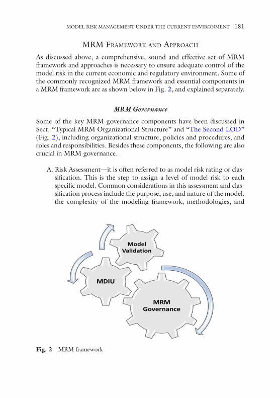
MRM FRAMEWORK AND APPROACH As discussed above, a comprehensive, sound and effective set of MRM framework and approaches is necessary to ensure adequate control of the model risk in the current economic and regulatory environment. Some of the commonly recognized MRM framework and essential components in a MRM framework are as shown below in Fig. 2 , and explained separately.

MRM Governance

Some of the key MRM governance components have been discussed in Sect. “Typical MRM Organizational Structure” and “ The Second LOD ” (Fig. 2 ), including organizational structure, policies and procedures, and roles and responsibilities. Besides these components, the following are also crucial in MRM governance.

A. Risk Assessment—it is often referred to as model risk rating or clas-sifi cation. This is the step to assign a level of model risk to each specifi c model. Common considerations in this assessment and clas-sifi cation process include the purpose, use, and nature of the model, the complexity of the modeling framework, methodologies, and

Fig. 2 MRM framework


implementation (which may indicate the probability of model error), as well as the impact of the model outputs and results (which could be the impact on the entity’s fi nancial results, regulatory compliance, and/or other aspects).

B. Model Inventory—MRM framework needs to include a compre-hensive inventory of the entity’s models, based on the defi nition and classifi cation of models stipulated in the policies and proce-dures. 8 The model inventory should include the key information pertaining to the models that is necessary to perform effective model risk management, such as:

• purpose, use and applicable products of the model; • brief description of the modeling framework, approach, and

methodologies; • model inputs (including type, data source, etc.), and feeder models

if applicable; • key model assumptions, including arithmetical (mathematical/sta-

tistical) assumptions and business assumptions; • model outputs, including adjustments/overlay to model outputs,

and downstream models; • model limitations, including restrictions on model use; • model governance/control details, such as versions, development/

delivery/update dates, risk rating or classifi cation, review and vali-dation schedule, policy exceptions, and so forth;

• contact information of the key stakeholders, including model owner, model developer, model user, and model validator.

• any changes to the model inventory should be closely monitored and tracked, and there should be a procedure to perform regular review, confi rmation and updates of the model inventory. Any new model development, model change, or model retirement should be accurately and promptly refl ected in the model inventory.

C. Issue/Status Tracking——there should be a robust procedure to manage the issues, that is, non-compliance with MRM policies and procedures, identifi ed during the MRM review and monitoring process (such as the issued identifi ed from model validations). Such procedures should include clear guidance regarding risk assessment of the issues, management response protocol, issue tracking and monitoring (including timetable, which often is dependent on issue

182 D.(T.) YANG

risk assessment), escalation procedures, resolution review, and issue status update.

D. Risk Reporting—on a periodic basis, for example monthly, quar-terly, and no less frequent than annually, the MRM group should provide model risk reporting to the senior management (which may be the oversight risk committees and/or the board of directors). The report should provide a clear depiction of the entity’s model risk state and profi le, and may include such information as impor-tant model additions/retirements, high-risk model issues identi-fi ed, model risk compliance status, key recommendations, and so on. Special attention should be paid to the aggregate model risk, which is measured and reported based on MRM’s review and analy-sis of the overall model risks with the consideration of linkage among models (i.e. the “correlated model risks”), which cannot be easily assessed by reviewing and validating individual models.

Model Development, Implementation, and Use (MDIU)

MDIU is usually conducted by the fi rst LOD, the roles and responsi-bilities of which (including the distinctions among model owners, model developers and model users) was discussed in Sect. “ The First LOD ”. From a MRM perspective, the key components in the MDIU process can be illustrated as following (Fig. 3 ).

Fig. 3 Model development, implementation and use


A. Business and functional requirements—it is the fi rst step in MDIU, which usually requires the model developer to: under-stand current state of process/environment; develop and docu-ment the business and functional requirements of the model; obtain and document formal business approval of requirements; and obtain reviewer signoff. In this step, the following considerations are important in defi n-

ing the business requirements—objective and scope of the model; use and purpose of the model; constraints/limitations of the model; reporting requirements; and intended audience.

Moreover, the functional requirements are important due to the following considerations: inputs, outputs, and processing compo-nents; core functions; alternative architectures; software capacity and versions; system capacity and database interface; and model control (security, user level defi nitions, access right, change control, version control).

B. Technical design and specifi cations. In this step, the following should be achieved: develop the tech-

nical design and model specifi cations; obtain reviewer approval and business client approval of technical design and specifi cation.

In drafting the technical design document, model developers should consider factors such as structure of the model, logic and process fl ow in the model, use of programming codes, error detec-tion, data elements, and user interface designs.

C. Model building—in this step, the model design and specifi cations are executed to build the model, which usually includes a few steps:

• coding and programing—creating model design and build plan, creating pseudocode or similar documentation of logic fl ow, and coding and programming the model based on business, func-tional, and technical requirements;

• performing alpha testing; • defi ning and establishing related model development control con-

stituents, including version and change control; • creating model documentation.

D. Model testing—this testing is focused on the functional perfor-mance and business acceptability, and usually includes the following steps:

184 D.(T.) YANG

• developing test plan/procedures (and obtaining formal business signoff on test plans if needed);

• performing testing per test plan/cases and documenting the test-ing results. The testing should include mathematical/statistical testing (e.g. sensitivity tests, stress tests, statistical assumptions tests, etc.), implementation and system testing, and user accep-tance testing, and so forth, when applicable;

• performing parallel testing, if necessary and appropriate; • analyzing test results, resolving errors and/or modifying model

accordingly, and documenting any changes.

E. Model implementation and deployment—this is the “last but not least” step, which is achieved through the following:

• obtaining signoffs from various stakeholders, including model reviewers and users;

• defi ning detailed process of implementation; • executing model implementation and deployment, which usually

includes transfer of the development code and documentation to the production team, additional coding if production is operated in a different system/environment, and so on;

• establishing, or assisting to establish, a comprehensive set of ongoing monitoring and tracking procedures.

• Model implementation and deployment is often not the end of model developers’ responsibilities, as they will frequently need to continue to play a key role in the model use down the road, and provide guidance or advice on many model control components such as model change and updates, version control, ongoing M&T, and so on.

F. Model use—after model development and implementation, the model can be used in production. However, model use should not be considered as simply an operational process—as a critical compo-nent of the MRM framework, it should proactively provide valuable feedback and input to facilitate continuous monitoring and enhancement of the model. From using and operating the model, the model users should try to contribute to MRM in at least the following ways:


• provide productive and constructive feedback and insights regard-ing the model functions and performance, leveraging the model user’s knowledge and experience in the specifi c business areas;

• conduct (or assist to conduct) the ongoing monitoring and track-ing procedures and controls, and assess the continuous applicabil-ity and appropriateness of the model based on the analysis the ongoing M&T results;

• monitor the model purpose and limitations regarding the model use, to ensure that the models are used as intended and permitted;

• provide challenges to the model developer/owner, and recom-mendations regarding updates and enhancement to the model, based on business results including changes in the market and industry conditions and environment—this is especially important when there are limited quantitative approaches (e.g. backtesting) to measure model performance;

• Determine and justify, any adjustments to model results (e.g. management overlays), such as those to address conservatism considerations.

Model Validation

Within the whole MRM framework, the model risk management group/department is considered as the heavy lifter, in terms of performing their full-time responsibilities to ensure that the MRM framework is well estab-lished, properly executed, and regularly monitored. One of the MRM group’s most important (and often the most onerous) duties is model validation, which is the focus of this section.

Per SR 11-7 / OCC 2011-12, an effective validation framework should include “three core elements:

• Evaluation of conceptual soundness, including developmental evidence

• Ongoing monitoring, including process verifi cation and benchmarking

• Outcomes analysis, including back-testing”. 9

This guidance, directive in nature, does not provide many details for proper execution of model validations, and inevitably is subject to interpretation.

186 D.(T.) YANG

One of the generally acceptable model validation structures is as depicted below (Fig. 4 ).

The components in a comprehensive and sound model validation are discussed in detail below.

Model Control and Governance The model validation should assess the model control governance and procedures, including model change control, implementation, and sys-tem (security, access controls, etc.), model use controls (e.g. input/out-put review and approvals), and so on. The model control and governance should be assessed with the reference and benchmark of the entity’s MRM policies and procedures.

Model Theory, Design, and Assumptions The model theory, design, approach, and key assumptions should be thoroughly reviewed and tested, based on which the model’s conceptual soundness needs to be assessed. The validation team should not take the current modeling framework and methodologies as a given, but should conduct extensive analysis, benchmarking to industry practice (both

Fig. 4 Model validation structure


common practice and leading practice) as well as academic research when-ever possible. Alternative methods should be widely considered and evalu-ated against the current modeling approach.

When reviewing model design, theory, approach, and key assump-tions, and assessing the conceptual soundness of the model, adequate model developmental evidence should be obtained. This should include not only quantitative evidence (data, code, formulas, etc.) but also qualitative evidence (business intuition, management’s input, etc.). The model limitations, both self-identifi ed and disclosed by model owner, and revealed by the validation team, should be carefully vetted and con-sidered in evaluating potential alternative approaches which may miti-gate such limitations.

Conceptual soundness can be reviewed, tested, and assessed in vari-ous ways, a few examples of which include literature review (model documentation, industry, regulatory, academia, etc.), benchmarking, exploratory data analysis (EDA)/confi rmatory data analysis (CDA), and outcome analysis.

Model Input, Processing, and Outputs The model input, processing, and output are also a key part of a model validation. Usually this step covers at least the following key components:

• data management and processing (e.g. data cleaning, data transfor-mation, data analysis);

• suitability of the data supplied to the models; • reasonableness of qualitative adjustments, if any; • accuracy of model calculations/formulas; • appropriateness of model functionality; • outcome analysis; • comprehensiveness and informativeness of output reporting.

For proprietary models (i.e. “in-house” models), this step is the bridge between theoretical design and framework and the execution of model development. The focus should be on model development process and practice, especially when the model validation is the initial (usually “full- scope”) validation before productionization of the model. For exam-ple, the data component will be primarily referring to the model fi tting

188 D.(T.) YANG

data, and the tests on data usually focus on the suitability (e.g. statistical properties, applicability to model purpose and use) of the data used to develop the model, to answer such questions as:

• The model is built on the assumption of normally distributed residu-als—does the model fi tting data fi t with that assumption?

• The volatility needs to be calibrated using ATM caps/fl oors/swap-tions—are the instruments used in the calibration appropriate?

• The model developer applied Akaike’s Final Prediction Error (FPE) technique to account for the larger variance in future forecasts than noted in the in-sample data—is this a reasonable practice considering the purpose of the model?

• The model fi tting data is transformed by taking the fi rst difference of the level data to achieve stationarity in a time series model—is that transformation successful (e.g. presence of a unit root after the transformation)?

By way of contrast, for vendor models, many such questions cannot be answered, since the model development/fi tting process is often a “black box” without access granted to the model validators. However, with a switched focus there is still plenty that can be done to validate these com-ponents of the model. Also taking the input data as an example, most usu-ally the focus will now be on the side of model use, with such questions as:

• The ALM model needs General Ledger (GL) data to be input to run in different interest rate scenarios—are the input data used in the model reconcilable to the source data originally from GL?

• The contractual terms of trades are needed as inputs to run the valu-ation model—were these data accurately inputted into the model?

• Were the market data, such as the LIBOR/swap curve, volatility sur-face, and such like correctly obtained (the correct curves and data, the correct “as of” date)?

• Were the inputs from other departments (e.g. deposit run-off esti-mates, new volume forecasts, etc.) reasonable and up-to-date? And so forth.

Needless to say, one cannot expect a uniform set of model validation procedures and steps to be applicable to all models. The model validators


must have the capability to understand the nature and characteristics of different models, and adjust the review and testing plans accordingly.

Outcome analysis is specifi cally called out in SR 11-7, which highlighted the necessity and particular importance of aligning the model results to both the business reality and the model purpose and use. Outcome analy-sis may include backtesting/out-of-sample testing, 10 sensitivity/scenario testing, stress testing, quantitative and business performance metrics, and so on. Outcome analysis is often straightforward to understand and per-form; however, the following are worth noting:

• It is important to establish the formal procedures and criteria of out-come analysis, including pre-determined, appropriate thresholds for the testing results, as well as an issue resolution process;

• Outcome analysis should be carefully designed and executed, based on the purpose, design, and implementation of the models. For example, the backtest period for a mortgage prepayment model could be three, six or twelve months, while that for a trading VaR model usually is 250 days;

• Some outcome analysis, such as backtesting, is not applicable to, or cannot be reasonably done for, all models (such as the valua-tion models of illiquid products, or many of the credit risk mod-els), and therefore alternative approaches should be considered (e.g. simulation- based testing);

• Outcome analysis should not be considered and conducted as a “one- time” test only as part of the initial model validation, but should be one of the most important tasks of ongoing model monitoring and tracking activities performed on a regular basis.

Model Implementation Model implementation refers to the process to actually “build” the model. This process can include the following items: model confi guration; cod-ing/programming and debugging; deployment and production of the model; installation, customization, and confi guration of vendor models; and various testing activities on the functionality of the model.

Clearly the implementation of the model directly affects and determines its functionality and suitability, and the defects in the model implementa-tion process may lead to improper use of the model, even if the model was designed well. Therefore, it is important to review and ensure that model

190 D.(T.) YANG

implementation has been appropriately conducted, with at least the fol-lowing verifi ed during the model validation:

• the codes are accurate and serve the model design; • model confi guration and model parameters set-up are proper; • system/IT framework is appropriate for the model; • testing done during the implementation process (e.g. parallel run-

ning) is well designed and performed, and the results are properly tracked and analyzed.

Model Ongoing Monitoring and Tracking Within the MRM framework, ongoing M&T serves as an independent function to monitor key model risks, with an appropriate frequency. This is a key model risk control to verify that the model performs as expected, and to ensure continuous applicability and appropriateness to use the model with the changing economic and business conditions. This responsibility usually lies within the fi rst LOD, owned by the model owners/users, and in certain cases by model developers.

The ongoing M&T can help capture the impact on the performance of the model from changing business environment, including changed prod-ucts, macroeconomic conditions, business and risk exposures, and so on, as well as new empirical evidence (e.g. additional observed business data) or recent academic research. Based on such impacts, the model owner may determine whether any updates, adjustments, or redevelopment/replace-ment of the model are warranted. For example, if new types of fi nancial derivatives start to be traded by the entity, the use of the existing trading VaR model may need to be reviewed; if adequate additional data points have been observed since the development of a regression-based PPNR model, then the model may need to be refi tted, and so on.

Outcome analysis is often a key part of the ongoing M&T activities. Backtesting, and other similar testing that is suitable based on the model’s nature and purpose, are usually an effective way to assess ongoing model performance, and a necessity to adjust model design, setting, and param-eters. For example, if a three-month backtest of the mortgage prepayment model shows large variances between forecasts and actuals, then adjust-ment to the prepayment tuning factors should be considered.

As part of the ongoing M&T, it is also important to monitor if any of the known model limitations have been breached in model use. For example, if a valuation model is known to have the limitation of static


interest rate term structures, while it was used to price American swaptions which require stochastic term structures, then this should be identifi ed and reported as a breach of the model limitations.

From a model validation perspective, it is also important to ensure that the ongoing M&T is properly designed and executed, by verifying such components as:

• there is a comprehensive and suitable ongoing M&T plan in place, including the appropriate frequency;

• the ongoing M&T plan has been executed properly, with support-ing evidence (not applicable for initial model validation before production);

• the ongoing M&T tests and procedures are appropriately designed and conducted;

• the testing results are thoroughly analyzed, reasonably interpreted, and the conclusions are properly drawn and adequately supported;

• any adjustments/overlays to model outputs are properly supported; • ongoing M&T results and conclusions are properly reported and

communicated to the entity’s MRM and management.

Ongoing M&T can be conducted in many different ways, such as per-formance measurement and assessment (e.g. backtesting), model refi tting, periodical process verifi cation and review, and benchmarking.

For certain types of models, the ongoing M&T may also include the “operational” tests, to periodically review and test the operational feasibil-ity of certain key assumptions. For example, the tests on the feasibility of funding sources/needs under simulated scenarios (which could be tested internally or externally) for liquidity stress testing models are conducted in some leading industry practices.

• Last but not least, MRM professionals should be fully aware of the fact that ongoing M&T varies signifi cantly across different types of models, and one uniform set of procedures and templates is usually not implementable for all models. For example, the model owner of an ALLL model may be completely confused by the ongoing M&T requirements for the model owner of a capital stress testing model developed based on time series regression. The model validators should be adequately fl exible to design and execute different testing procedures on ongoing M&T for various kinds of models.

192 D.(T.) YANG

Risk Rating One of the key outcomes of model validation is the assessment of whether the model is appropriately built for its intended purpose and use, which, in other words, means that the model validation must provide a clear assess-ment of the level and nature of the risks of using the model in production. Such risk ratings need to include the rating for both the specifi c fi ndings and issues identifi ed during the course of model validation, as well as the assessment of the overall risk associated with the model as a whole.

The MRM policies and procedures should have a clear defi nition and guidance of model risk assessment and rating, which most often are driven by the nature, cause, and impact of the fi ndings on model performance. For the risk rating of fi ndings/issues, the considerations may include whether the issue pertains to the fundamental model theory, design, and other key modeling components such as assumptions, inputs, and process-ing; whether the issue is the result of signifi cant lack of model controls; what is the impact of the issue on the overall model performance; and so on. The risk rating, once determined, should also be the basis of the resolution plan, including the necessity and time limit for model owner’s response and remediation.

The overall model risk assessment is the result of aggregating the issue risks and evaluating the risk of the model as a whole. This provides the model owner and the management with a comprehensive opinion and conclusion regarding the risks to use the model for its designated pur-poses. Such assessment may result in different levels of overall model risk ratings, such as the following:

• “Acceptable”—which usually means the issues identifi ed from model validation, if any, are minor, and the model overall is sound and per-forms as expected;

• “Conditionally Acceptable” (or “Acceptable with Limitations”)—which usually means that overall the model can be used, but before its use there are certain conditions to be met, or limitations to be remediated, such as resolution of certain issues;

• “Rejected”—which usually means that the model is fundamentally defi cient, and does not meet the requirements for its designated use (and redevelopment or replacement of the model may be necessary);

• “Restricted Use”—which usually means the model should not be used for production, but may be used for other purposes, such as to serve as the benchmark (or “challenger”) model;


• “Inconclusive” (or “Unable to Validate”)—which usually means that there are signifi cation limitations, such as unavailability of adequate developmental evidence, that made it unfeasible to perform the vali-dation, and therefore the assessment cannot be performed.

• Again, the defi nitions and guidance regarding model risk assessment and rating should be clearly provided in the MRM policies and pro-cedures. Model validations should strictly follow these defi nitions and guidance in the execution of risk rating.

Effective Challenge Another key output and core purpose of model validations is to provide effective challenges. “Effective challenge” is a broad concept. As defi ned in SR 11-7 / OCC 2011-12, it is the “critical analysis by objective, informed parties who can identify model limitations and assumptions and produce appropriate changes”. 11

Effective challenges are “challenges”, meaning that the activities and results should be aimed to identify defi ciencies and risks in the model, and to question the appropriateness to use the model for its designated pur-poses, rather than supporting the current model (or “window-dressing”). And these challenges need to be “effective”, meaning that any defi ciencies and issues identifi ed during the challenging process should aim to refl ect, in a meaningful way, the true risks associated with the model develop-ment, model implementation, and model use; it also means that the par-ties who provided the effective challenges need to have adequate infl uence and authority to enforce serious consideration of, and necessary response to, the challenges raised.

Effective challenges should be the principle in MRM activities con-ducted by all the three LOD within the MRM frame work—for exam-ple, the business user should provide adequate effective challenges to the model developer, as the effective challenges within the fi rst LOD. For model validators, this certainly is also the key principle to keep in mind.

Effective challenges may be raised on all the key model components, such as the following:

• model design framework—example challenge: whether OLS is an appropriate framework while auto regressive models are more often used in the industry;

• model methodologies—example challenge: stochastic terms struc-ture may generate better model performance than static terms struc-

194 D.(T.) YANG

ture currently used by the model; or the Nelson-Siegel model may be a better yield curve smoothing methodology than the current cubic spline method;

• model inputs—example challenge: how to justify the use of industry data rather than the entity’s internal data to fi t the model;

• key assumptions—example challenge: whether the deposit growth assumptions are reasonably developed for the ALM models;

• outcome analysis—example challenge: the methodologies, including the designed scenarios, for the sensitivity tests conducted during the model development process may not be reasonable, or a “global” sensitivity test may generate more meaningful and enlightening results than the “local” sensitivity tests conducted by the model developer;

• model reporting—example challenge: the reporting package of the model (e.g. IRR report package for ALCO) may also need to include additional information, based on industry leading practice;

• ongoing M&T—example challenge: the threshold for fl uctuation of coeffi cients from periodical model refi tting is set to be a fi xed num-ber, while it may be more meaningful to use the standard error of the coeffi cients as the basis to set the thresholds, considering the large differences among the coeffi cients;

• model control—certain model control procedures should be estab-lished or modifi ed considering the nature and risk of the model; and so on.

Obviously, there are many different ways to raise effective challenges during the course of model validation, which include (but are not limited to) the following:

• benchmarking and referencing the modeling approach and process to industry practice, as well as academic research;

• analyzing the model risks, based on a thorough understanding of each key modeling component, along with the model purpose and use, to identify any gaps;

• perform exploratory analysis (including building benchmark models when necessary and appropriate) on alternative modeling framework and methodologies;

• analyzing and assessing the model developer’s interpretation of testing results and conclusions against the evidence;


• conducting additional testing to identify the potential defects, and thus misleading results, of the model testing performed by the model developer; and so on.

• To summarize, model validation is the key part of continuous MRM practice. It requires an extensive skill set in fi nancial modeling and quantitative analytics, and solid business knowledge, as well as a thor-ough understanding of risk management principles and concepts. The competence and capability requirements for qualifi ed model validators are usually no lower than those for the model developers or business managers.

CONCLUSION As discussed in this chapter, revolutionarily improved model risk man-

agement practice has been a direct outcome from the lessons learned by the market practitioners in the recent fi nancial crisis. This mission is com-plex and long-term in nature, with an onerous process involved to accom-plish. As mentioned, the effort to build, enhance, and refi ne the MRM practice is still underway, with new challenges arising almost on a daily basis in this ever-evolving economic, business and market environment. At the end of the day, a sound MRM is expected to play a key role in the overall risk management, to help prevent similar crunches from occurring again in the fi nancial services industry.

NOTES 1. SR 11-7/OCC 2011-12, Page 3, Para. 1. 2. The common practice of banks’ capital stress test involves numerous com-

ponent models to cover different stress testing factors (such as credit risk of different products/portfolios, operation risk, market risk, as well as the pre-provision net revenue (PPNR) forecasts), and the results from these component models are then “integrated” to calculate the fi nal stress test results under different stressed scenarios. Banks often utilize their asset liability management (ALM) systems to perform such integration, but the approaches, methodologies and procedures largely vary.

3. SR 11-7/OCC 2011-12, Page 3, Para. 3. 4. SR 11-7/OCC 2011-12, Page 18, Para. 5. 5. CCAR banks refers to the bank holding companies that are subject to the

comprehensive capital analysis and review (CCAR), which is an annual

196 D.(T.) YANG

review conducted by the Federal Reserve, and are usually the banks with greater than $50 billion in consolidated assets; the DFAST banks refers to the bank holding companies, excluding the CCAR banks, that are subject to the Dodd-Frank Act stress testing (DFAST), which usually have $10~50 billion in consolidated assets.

6. SR 11-7/OCC 2011-12, Page 19, Para. 2 7. Sarbanes–Oxley Act of 2002, aka the “Public Company Accounting

Reform and Investor Protection Act”. 8. In some entities, the MRM group may also be required to develop, main-

tain, and monitor the inventory of other (“non-model”) tools, such as user-defi ned tools (“UDT”) or end-user computing (EUC) tools. In such cases, there usually should be a separate risk management framework and approaches on these non-model tools.

9. SR 11-7/OCC 2011-12, Page 11, Para. 1. 10. Theoretically backtesting and out-of-sample testing have different defi ni-

tions, although they serve similar purposes (testing the model fi tness based on observed data). However, in the industry, out-of- sample tests were often referred to as “backtests” due to the different understanding and interpretation of these terms.

11. SR 11-7/OCC 2011-12, Page 4, Para. 4.


CCAR and Stress Testing


Region and Sector Effects in Stress Testing of Commercial Loan Portfolio

Steven H. Zhu

S.H. Zhu (*) New York, USA

The view expressed in this paper represents the personal opinion of author and not those of his current and previous employers.

IntroductIon

The estimation of future loan losses is not only important for financial institutions to effectively control the credit risk of a commercial loan port-folio, but also an essential component in the capital plan submitted for regulatory approval in the annual Comprehensive Capital Analysis Review (CCAR) and Dodd-Frank Act Stress Test (DFAST) stress testing.1 Under the regulatory guidelines, banks must demonstrate in their stress testing methodology that the risk characteristics of loan portfolio are properly captured at a granular risk-sensitive level to adequately reflect the region and sector effects2 when incorporating the impact of macroeconomic sce-narios. This chapter describes a methodology of estimating the point-in- time (PIT) default probability that can vary according to macroeconomic scenarios and at the same time capture the credit risk at the region and industry sector levels using external rating agency data. The key to this modeling approach is the maximum likelihood estimation of credit index and correlation parameters calibrated to the historical default and rating

202

migration data. The credit index3 in the model represents the “hidden” risk factor underlying the default while the correlation parameter can be attributed to the default clustering, and the estimation of credit index and correlation provides a compelling explanation for the original design of risk-weight function used in the calculation of credit risk capital charge in the Pillar 1 of Basel II capital rule. The methodology can be used as a benchmark model to validate the bank’s internal model, because it can be built in compliance with the bank’s internal risk rating system and it can also be implemented with external data from the rating agency such as S&P and Moody’s, thus making it practical for many institutions with only limited internal data on default and migration history.

How the probability of default and rating migration responds to changes in the macroeconomic environment are important for banks to assess the adequacy of credit risk reserve and capital adequacy under nor-mal and stressed market conditions. Credit reserve and capital are pri-mary tools for banks to manage and control the credit risk in their loan portfolios,

– credit reserves are designed to cover the expected losses which are predicted to be experienced in the bank’s loan portfolio over the normal economic cycle;

– credit capital is designed to cover the unexpected loss which only occurs under a downturn economy or in extreme market conditions.

Banks are required under Basel II rules to develop through-the-cycle (TTC) probability of default (PD) model for estimating credit reserve and capital requirement. Banks have used a wide range of methods to estimate credit losses, depending on the type and size of portfolios and data avail-ability. These methods can be based on either accounting loss approach (i.e. charge-off and recovery) or economic loss approach (i.e. expected losses). Under the expected loss approach, the losses are estimated as a function of three components: probability of default (PD), loss given default (LGD), and exposure of default (EAD). In general, banks can apply econometric models to estimate the losses under a given scenario, where the estimated PDs are independent variables regressed against the macroeconomic fac-tors and portfolio or loan characteristics. However, econometric models are often based on data availability which can be problematic in practice to PD estimation on a low-default and investment-grade portfolio such as large commercial and industrial (C&I) loans.4 Hence, banks sought out

S.H. ZHU

to develop a structural approach to model the probability of default and rating transition in order to estimate and predict the future losses on such portfolios.

In this chapter we employ a rating transition-based approach, called “credit index model”, to produce a stressed transition matrix for each quarter, which is forward-looking and can be used to estimate the credit losses for the wholesale portfolio under stress scenarios. This chapter can be viewed as an introduction to CCAR stress testing of a commercial bank with large commercial loan portfolios.

Specifically, the approach can be built on the bank’s internal rating sys-tem or external rating agency system to project how the obligator ratings could change over time in response to the change of macroeconomic sce-narios. The detailed process of model implementation has the following characteristics.

(1) Represent the rating transition matrix as a single summary measure called “credit index”;

(2) Estimate a time-series regression model linking the credit index to the scenario variables;

(3) Project credit index over the multiple quarterly planning horizon from the time-series model;

(4) Transform the projected credit index into a full sequence of quar-terly transition matrices.

The calibration of the credit index model is based on the S&P historical default and transition data covering the 30-year period from 1981 to 2011. After the construction of the credit index, we perform the statistical regres-sion analysis to establish the relationship and model the credit index in rela-tion to the 26 macroeconomic variables provided in 2013 CCAR so that we can project the future values of credit indices in each of three regions based on their respective macroeconomic drivers (such as GDP, CPI, and/or Unemployment), and the projected values of credit index are properly matched in time step to produce the stressed PDs and transition matrices in each of two years in the planning horizon under the CCAR macroeconomic scenarios. Finally, we provide the results of backtest analysis to compare the modeled PDs with the default experiences over same 30-year historical period.

The credit index model is an adoption of the Credit Metric approach based on conditional probability. Compared to the unconditional approach, the conditional approach captures the credit cycle of economy

REGION AND SECTOR EFFECTS IN STRESS TESTING OF COMMERCIAL LOAN... 203

204

modeled as the systematic risk factor (i.e. credit index) and the correla-tion of individual obligor’s default with the systematic factor. The higher correlation implies higher levels of probability of default and more down-grade transition from the high ratings to the low ratings. The importance of a conditional approach in modeling the default and transition matrix is highlighted in the 1999 BCBS publication [1] and recent FRB guideline [4] with an emphasis on its ability to improve the accuracy of the credit risk models. Hence, the use of the Credit Metrics approach to model the credit index as described in this chapter is consistent in a general effort to better aligning the firm’s CCAR stress testing approach with the firm’s overall credit stress test framework.

EstImatIon of crEdIt IndEx and dEfault corrElatIon

This section explains first the estimation of credit index and default corre-lation. Banks often develop their own internal rating system for credit risk management, where the internal ratings are normally based on the score-card model to assess the creditworthiness of obligors, and then derive the rating-based probability of default (PD) based on the long-term annual transition matrix (such as one in the following Table 1), which are mapped internally at the obligor level for the purpose of evaluating credit exposure, credit reserve, and credit capital management. Hence, the change in credit quality of a loan portfolio under a macroeconomic shock (such as the one in the CCAR stress scenario) may be quantified by modeling the effect of such economic shock on the probability of default and rating migration.

Table 1 S&P historical average transition matrix over 30 years (1981–2011)

MS.NA AAA AA A BBB BB B CCC D

AAA 88.81 10.50 0.49 0.06 0.13 – 0.02 –AA 0.55 90.20 8.34 0.68 0.10 0.09 0.02 0.02A 0.05 1.88 91.36 5.90 0.51 0.17 0.04 0.08BBB 0.02 0.18 4.31 89.43 4.78 0.93 0.12 0.23BB 0.02 0.07 0.32 6.08 83.08 8.44 0.80 1.18B – 0.05 0.25 0.39 5.92 83.68 4.41 5.30CCC – – 0.34 0.34 0.90 13.06 57.16 28.21

S.H. ZHU

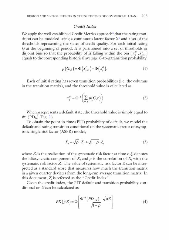
Credit Index

We apply the well-established Credit Metrics approach5 that the rating tran-sition can be modeled using a continuous latent factor X6 and a set of the thresholds representing the states of credit quality. For each initial rating G at the beginning of period, X is partitioned into a set of thresholds or disjoint bins so that the probability of X falling within the bin [ xg

G , xgG+1 ]

equals to the corresponding historical average G-to-g transition probability:

p G g x xg

GgG,( ) = ( ) − ( )+Φ Φ1 .

(1)

Each of initial rating has seven transition probabilities (i.e. the columns in the transition matrix), and the threshold value is calculated as

x p G rgG = Φ− ∑1 ,

r g<( )

(2)

When g represents a default state, the threshold value is simply equal to Φ−1(PDG) (Fig. 1).

To obtain the point-in-time (PIT) probability of default, we model the default and rating transition conditional on the systematic factor of asymp-totic single risk factor (ASFR) model,

X Zt t t= ⋅ + − ⋅ρ ρ1 ξ (3)

where Zt is the realization of the systematic risk factor at time t, ξt denotes the idiosyncratic component of Xt and ρ is the correlation of Xt with the systematic risk factor Zt. The value of systematic risk factor Z can be inter-preted as a standard score that measures how much the transition matrix in a given quarter deviates from the long-run average transition matrix. In this document, Zt is referred as the “Credit Index”.

Given the credit index, the PIT default and transition probability con-ditional on Z can be calculated as

PD g ZPD ZYR|( ) = ( ) −

−

−

ΦΦ 1

1

1

ρ

ρ

(4)


206

p G g Zx Z x Z

tgG

t gG

t,| ,|( ) =−

−

−

−

−

+Φ Φ1

1 1

ρ

ρ

ρ

ρ.

(5)

This is the model value at the quarter t of the g-rated PD and G-to-g transition in one year’s time from the quarter t.

Next, we apply two alternative MLE-based methods to calibrate the quarterly value of credit index from historical default and migration prob-ability during 1981–2011.

1. Credit index calibrated to the whole transition matrices

max ., ,Z t G g t

G gt

n Ln p G g Z∑∑ ⋅ ( ) , ,|

(6)

Rat ing AAA AA A BBB BB B CCC

AAA (2.46) (2.87) (2.98) (3.61) (3.61) (4.75)

AA (1.33) (2.36) (2.82) (2.99) (3.31) (3.52)

A 2.07 (1.50) (2.41) (2.76) (3.04) (3.15)

BBB 2.89 1.70 (1.55) (2.23) (2.69) (2.83)

BB 3.12 2.64 1.51 (1.26) (2.06) (2.26)

B 3.29 2.75 2.46 1.51 (1.30) (1.62)

CCC

(1.22)

2.54

3.26

3.57

3.56

4.75

6.60 6.60 2.71 2.47 2.15 1.05 (0.58)

BBB

Firm remainsBBB

CCC

Default

Lower Higher

BB

AA

AAA

B

A

Fig. 1 Partitioning of rating transition matrix

S.H. ZHU

2. Credit index calibrated to the PD-only last column in the transition matrices

max , , ,Z t g t t g t g t

gt

n Ln p g Z N n Ln p g Z∑ ⋅ ( ) + −( ) ⋅ − ( ) ( )| |1

(7)

where nt , G , g = transition count at time t from G-rating to g-rating, Nt , g = total count at time t of g-rated obligors and nt , g = default count at time t of g-rated obligors. The time series of credit index Zt is estimated from the quarterly history of one-year default/transition matrix data during 30-year time period (1981–2011).

For the purpose of the CCAR stress test, we choose to calibrate the credit index only to the default column of transition matrix. The diagram in Fig. 2 provides a graphic illustration of the quarterly estimation pro-cess. For each quarter, we calculate the one-year rating transition matrices7 from 1981Q1 to 2012Q3. We apply the maximum likelihood estimation (MLE) to estimate the value of global credit index Z at each quarter and obtain a time series of Zt(ρ) from 1981Q1 to 2011Q4 as shown in the following diagram.

The estimation of correction parameter ρ is based on the Basel II-IRB representation as follows

ρ ρ= ⋅ + −( ) 0 1 50exp *PDAvg

(8)

where PDAvg = the historical average probability of default per rating. The correlation parameter ρ plays an important role in the Basel’s credit risk- weight function model under Basel II and Basel III [2] as it controls the proportion of the systematic risk factor Zt affecting the set of loans in the economy.8

To obtain the industry and region-specific credit index, we repeat the iteration steps described above and calibrate the index in each historical quarter based on the cohort pool of defaults (and migration) observed only within the region or industry to obtain the credit index for a major industry sector such as financial institutions or a region such as the USA, Europe, and Asia (developing nations), respectively.


208

#Qtr

TIM

E HO

RIZO

NCR

EDIT

INDE

X

Ra n

gAA

AAA

+…

.CC

CD

AAA

AA+

… CCC

D

Ra n

gAA

AAA

+…

.CC

CD

AAA

AA+

… CCC

D

Ra n

gAA

AAA

+…

.CC

CD

AAA

AA+

… CCC

D

. . .

. .

. . .

. . .

. .

. . .

. . .

. .

. . .

. . .

. .

. . .

. . .

. .

. . .

. . .

. .

. . .

. . .

. .

. . .

. . .

. .

. . .

. . .

. .

. . .

. . .

. .

. . .

. . .

. .

. . .

. . .

. .

. . .

. . .

. .

. . .

. . .

. .

. . .

. . .

. .

. . .

. . .

. .

. . .

Ra n

gAA

AAA

+…

.CC

CD

AAA

AA+

… CCC

D

Z12

3(Q

4 20

11 -

Q3

2012

)

1-Y

EAR

TRAN

SITI

ON

MAT

RIX

(BY

QUA

RTER

)

Q1

198

1- Q

4 1

981

Q2

198

1 -

Q1

198

2

Q3

198

1 -

Q2

198

2

Z1(Q

1 19

81-Q

4 19

81)

Z2(Q

2 19

81-Q

1 19

82)

Z3 (Q

3 19

81-Q

2 19

82)

1 2 3 123

Q4

201

1 -

Q3

201

2

Fig.

2

Qua

rter

ly it

erat

ion

of e

stim

atin

g cr

edit

inde

x Z

from

def

ault

and

tran

sitio

n m

atri

x

S.H. ZHU

Under the Credit Metrics approach, the credit index is a measure that represents how much the transition matrix deviates (in terms of upgrades and downgrades) from the long-term transition matrix. It can be shown that the credit index, when calibrated only to the default column of transi-tion matrix, will correlate better with the historical default rates (i.e. 73% with BB-rated and 92% with B-rated) and it also coincides with the three economic downturns in the 30-year history from 1981 to 2012 (Fig. 3).

The credit index admits a very intuitive interpretation as the value of Zt measures the “credit cycle” in the following sense:

– The negative values of Zt (<0) indicate the bad year ahead with a higher than average default rate and a lower than average ratio of upgrades to downgrades.

– The positive values of Zt(>0) indicate the good year ahead with a lower than average default rate and migration to the lower ratings.

Given the value of credit index, we can then apply the formula (5) to construct a transition matrix. As an example, let us look at two transi-tion matrices below corresponding to two particular values of the credit index Z = +1.5 and −1.5, with a fixed Rho-factor (ρ = 10%). We observe the large changes in the values of cells above diagonals representing the

0

2

4

6

8

10

12

14

16

18

20

-3

-2

-1

0

1

2

3

4

5

6

7

8

1-Ja

n-81

1-Ju

l-82

1-Ja

n-84

1-Ju

l-85

1-Ja

n-87

1-Ju

l-88

1-Ja

n-90

1-Ju

l-91

1-Ja

n-93

1-Ju

l-94

1-Ja

n-96

1-Ju

l-97

1-Ja

n-99

1-Ju

l-00

1-Ja

n-02

1-Ju

l-03

1-Ja

n-05

1-Ju

l-06

1-Ja

n-08

1-Ju

l-09

1-Ja

n-11

Credit Index BB-rated B-rated

Fig. 3 Historical default rate versus credit index


210

probability of one-notch downgrades, indicating the significant increases in downgrades when credit index Z changes from the positive state to the negative state (Table 2).

Default Correlation

The correlation (ρ) is used to capture how obligor-specific risk changes in relation to the systematic risk of the credit index as described in previ-ous section. The credit index was estimated in the previous section by assuming the correlation is known a priori. In this section, we describe an approach designed to estimate ρ independently from the credit index, by constructing a MLE function as the binomial distribution of default occurrences.

Specifically, we model the default as the Bernoulli event.9 For a given historical one-year period (indexed quarterly in time t), there are dt,s = #defaults out of Nt,s = #obligors in a cohort (c). Conditional on Z = Zt, the probability of default is given by

p g ZP Z

c t

g t| ;ρ

ρ

ρ( ) = ( ) −

−

−

ΦΦ 1

1

Table 2 Conditional transition matrix (Z = +1.5 and Z = −1.5)

Rating AAA AA A BBB BB B CCC D

AAA 98.23 1.74 0.02 0.00 0.00 – 0.00 0.00AA 1.81 96.89 1.26 0.03 0.00 0.00 0.00 0.00A 0.19 5.70 93.32 0.76 0.02 0.00 0.00 0.00BBB 0.06 0.59 11.69 86.94 0.66 0.06 0.00 0.01BB 0.06 0.23 0.99 14.47 82.03 2.01 0.10 0.10B 0.00 0.15 0.70 1.00 12.31 82.93 1.63 1.29CCC 0.00 – 0.92 0.86 2.08 23.26 59.48 13.39AAA 72.94 24.72 1.56 0.19 0.44 – 0.05 0.10AA 0.02 76.81 20.21 2.14 0.34 0.31 0.08 0.10A 0.00 0.12 82.28 15.01 1.61 0.57 0.13 0.28BBB 0.00 0.00 0.45 83.59 11.97 2.82 0.39 0.78BB 0.00 0.00 0.02 1.08 75.48 17.87 2.10 3.45B 0.00 0.00 0.03 0.06 1.64 78.63 7.96 11.67CCC 0.00 – 0.04 0.06 0.19 5.10 48.92 45.70

S.H. ZHU

Thus, the probability of observed defaults in this one-year period is given by the binomial formula

B ZN

dg Z p g Zc t

t g

t gc t

d

c t

N dt g t g t; | |ρ( ) =

( ) − ( )

−,

,

, ,p 1 ,,g

(9)

Hence, we obtain the unconditional log-likelihood function by inte-grating the binomial probability with respect to the credit index (Z) and then summing over all the quarterly one-year periods:

MLE B Z Z dZt c t t tρ ρ( ) = ( ) ⋅ ( ) ⋅∫∑ Φlog ;

(10)

The likelihood function is “unconstrained” because it is a function of only one parameter “Rho(ρ)”, and the integral of binomial distribution can be computed numerically using either simple Uniform method or Gauss-Hermite quadrature.10 The estimation of the correlation parameter (ρ) is simply the solution of MLE, that is, the point when the MLE func-tion reaches the maximum. For the entire population of S&P default data, the estimated value of correlation ranges from 9% to 13% depending on the period of default sample selected.

By applying such estimation methods to historical data in different sectors, we estimate ρ0 across a range of industrial sectors based on (10) as shown in Fig. 4. The same methodology can be used to obtain the estimation of correlation factors across the major regions: ρ0(US) = 12%, ρ0 15* %EU( ) = and ρ0 20* %EM( ) = .

EstablIshIng futurE crEdIt scEnarIos

As part of annual CCAR, the regulators often provide two stress scenar-ios (adverse and severely adverse) in addition to the baseline where each scenario starts in the fourth quarter of 2012 and extends for three years through the fourth quarter of 2015. The scenarios are defined for the same set of 26 macroeconomic variables that are provided to the banks subject to the stress testing requirement.

The main idea of the presented approach in this chapter is to model the credit index as the representation of credit risk in the bank’s loan port-folios, and thus applying regression analysis to establish the relationship


212

of the credit index with respect to the selected macroeconomic variables necessary to translate the CCAR macroeconomic scenarios to the stressed PDs and stressed transition matrices that can in turn be used to stress test the loan portfolios. Therefore, we shall next discuss the details of linking the credit index to CCAR macroeconomic variables.

Linking Credit Index to CCAR Macroeconomic Variables

The credit index Zt is a quarterly time series, and the value of Zt at time t represents the credit condition (i.e. default and migration) one-year ahead of time t because it is estimated from the historical defaults and rating transitions which occurred in the following year from the time t. Compared with the key economic indicator such as US GDP growth rate, it is shown in the graph below that the credit index is leading over GDP growth rate by two quarters during the three downturn years (i.e. 1990–1991, 2001–2002 and 2008–2009) in recent history. Hence, we can match the GDP growth rate by shifting the time step of credit index forward by two quarters.

There are 26 macroeconomic variables provided in 2013 CCAR [3], where fourteen of them are related to US economic conditions and the rest are representatives of Europe and Asian developing nations. Since the credit index is calibrated to measure the credit cycle predominately

13% 14%

10%

15%

22%

7%

-140

-130

-120

-110

-100

-90

-80

-70

-60

-50

-40

0.01

0.04

0.07

0.10

0.13

0.16

0.19

0.22

0.25

0.28

0.31

0.34

0.37

0.40

0.43

0.46

0.49 Rho(=ρ)

MLE(ρ)

FinancialInst itut ions/13.5%

Energy/14%

Industrials/9%

Materials/15%

Ut ilit ies/22%

Transportat ion/7%

S&P industry sectors

Consumer 7.0%14.0%13.5%

9.0%

9.0%9.0%

15.0%

15.0%

42.5%

24.0%

7.0%22.0%

12.5%

Energy

Financial Institutions

HealthcareIndustrials

Insurance

Leisure TimeMaterialsReal EstateTelecom

Transportation

UtilitiesInformation Technology

Rho (ρ)

Fig. 4 Rho (ρ) and MLE curve as function of (ρ) for selected industry sector

S.H. ZHU

related to the obligors in the US region, we perform a stepwise variable selection method to choose from fourteen US macroeconomic variables that are consistent with the economic rationale and at the same time sta-tistically significant based on the regression p-value statistics. The variables are selected in each case not only based on the statistical significance (i.e. p-value < 5%) but also with an interpretable sign on its coefficient (i.e. the slope of regression). The coefficients with +/− signs suggest the positive (negative) response of selected economic variables to the credit index, that is, the increases in these variables drive up (down) the value of credit index and thus produce the higher upgrade (downgrade) probabilities in the transition matrix.

For the regression analysis, we first need to shift the time step of the credit index forward by two quarters to match the GDP growth rate and then choose11 that we use more than fourteen-year quarterly data in the regression that covers two economic downturns during 1998Q1–2012Q1 as shown in Fig. 5. As a result, we obtain the regression of the credit index with the five selected macroeconomic variables:

C t a b t b t

b

USIndex USGDP USCPI

Mtge

growth rate

rat

( ) = ( ) + ( )+

+0 1

2

* *

* ee price

price

DJIA

House Residuals

t b t b

t

( ) ( )( )

+ +

+3 4*

*

(11)

Notice the GDP in the above graph is measured as a “year-over-year” (i.e. YoY) growth rate while the GDP data in CCAR is provided as a quar-terly “quarter-over-quarter” (i.e. QoQ) growth rate. Since credit index exhibits a serial correlation due to three overlapping quarters in the con-secutive quarterly values of credit index, we must first transform both GDP and CPI quarterly data in CCAR from the quarterly (QoQ) growth rate into the yearly (YoY) growth rate by compounding the four quarterly growth rates, which resulted in much smoother shape time series data of GDP growth rate and CPI quarterly rate. As a result, it can further enhance the statistical goodness-of-fit performance of regression analysis, as shown in following Fig. 6 for USA and Europe GDP YoY growth rates overlaid with the quarterly (QoQ) growth rates.

The right-hand graph above displays the fitted credit index relative to the historical credit index during the sample period of regression. As a result of data smoothing, credit index regression achieves remarkable


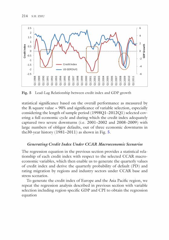
214

statistical significance based on the overall performance as measured by the R-square value = 90% and significance of variable selection, especially considering the length of sample period (1998Q1–2012Q1) selected cov-ering a full economic cycle and during which the credit index adequately captured two severe downturns (i.e. 2001–2002 and 2008–2009) with large numbers of obligor defaults, out of three economic downturns in the30-year history (1981–2011) as shown in Fig. 5.

Generating Credit Index Under CCAR Macroeconomic Scenarios

The regression equation in the previous section provides a statistical rela-tionship of each credit index with respect to the selected CCAR macro-economic variables, which then enable us to generate the quarterly values of credit index and derive the quarterly probability of default (PD) and rating migration by regions and industry sectors under CCAR base and stress scenarios.

To generate the credit index of Europe and the Asia Pacific region, we repeat the regression analysis described in previous section with variable selection including region-specific GDP and CPI to obtain the regression equation

-6

-4

-2

0

2

4

6

-2.5

-2

-1.5

-1

-0.5

0

0.5

1

1.5

2

2.5

Q1

1988

Q1

1989

Q1

1990

Q1

1991

Q1

1992

Q1

1993

Q1

1994

Q1

1995

Q1

1996

Q1

1997

Q1

1998

Q1

1999

Q1

2000

Q1

2001

Q1

2002

Q1

2003

Q1

2004

Q1

2005

Q1

2006

Q1

2007

Q1

2008

Q1

2009

Q1

2010

Q1

2011

GDP

Grow

th

Cred

it In

dex

Credit Index

US GDP(YoY)

Fig. 5 Lead-Lag Relationship between credit index and GDP growth

S.H. ZHU

-10

-8

-6

-4

-2

0

2

4

6

8

-5

-4

-3

-2

-1

0

1

2

3

4

5

2001

Q1

2001

Q4

2002

Q3

2003

Q2

2004

Q1

2004

Q4

2005

Q3

2006

Q2

2007

Q1

2007

Q4

2008

Q3

2009

Q2

2010

Q1

2010

Q4

2011

Q3

2012

Q2

2013

Q1

2013

Q4

2014

Q3

2015

Q2

US GDP YoY growth (2013 CCAR)

Base

Averse

Severely Adverse

GDP QoQ Growth

-2.5

-2

-1.5

-1

-0.5

0

0.5

1

1.5

2

2.5

2011

Q4

2011

Q1

2010

Q2

2009

Q3

2008

Q4

2008

Q1

2007

Q2

2006

Q3

2005

Q4

2005

Q1

2004

Q2

2003

Q3

2002

Q4

2002

Q1

2001

Q2

2000

Q3

1999

Q4

1999

Q1

1998

Q2

Credit Index Regression

Cindex

Cindex.Fi�ed

Fig. 6 2013 CCAR scenarios for USA and Europe GDP growth

216

C a b b t

b

EUIndex EUGDP EUCPI

Mtge

growth rate

rat

t t( ) = ( ) ( )+ +

+0 1

2

* *

* ee price

price

DJIA

House Residuals

t b t

b t

( ) ( )( )+

+ +3

4

*

*

(12)

where EUGDPgrowth is the EU GDP YoY growth rate and the graph below shows the quarterly projection of credit indices with respect to CCAR supervisory scenarios based on the regression equation for each credit index. Due to the data limitation and lack of variable selection, the regression performance12 of region-specific credit index can achieve an R-square at 80% in Europe and only about 65% for Asia and developing nations (Fig. 7).

While the historical pattern of the credit index depicts the past credit conditions in the history of the economic cycle, the levels of stress in CCAR scenarios are adequately captured and reflected in the projection of the credit index as translated by the statistical regression model.

strEssEd Pd and thE transItIon matrIx

This section describes the calculation of stress PDs and the transition matrix from the credit index under 2013 CCAR scenarios. The transi-tion matrix on whole grades can be calculated for three regions under each CCAR scenario using the formula (5) in the previous section, which uses the projected value of each region’s credit index in conjunction with the average transition matrix. Once the transition matrices are calculated, stressed PDs are simply the default column of the transition matrix. Both stressed PDs and transition matrices are expressed annually for 2013 and 2014 respectively, and the two-year stressed PDs (over 2013–2014) are derived from the two-year transition matrix which one obtains by multi-plying two one-year transition matrices.

Modeling the Transition Matrix on the Credit Index

Conditional on the state of the credit index, we are able to calculate the stress default probability (PD) for each region as follows

S.H. ZHU

-5

-4

-3

-2

-1

0

1

2

3

1998

Q1

1998

Q4

1999

Q3

2000

Q2

2001

Q1

2001

Q4

2002

Q3

2003

Q2

2004

Q1

2004

Q4

2005

Q3

2006

Q2

2007

Q1

2007

Q4

2008

Q3

2009

Q2

2010

Q1

2010

Q4

2011

Q3

2012

Q2

2013

Q1

2013

Q4

2014

Q3

2015

Q2

Credit Index -North America

NA-BaseNA-AdvNA-SAdv

-5

-4

-3

-2

-1

0

1

2

3

1998

Q1

1998

Q4

1999

Q3

2000

Q2

2001

Q1

2001

Q4

2002

Q3

2003

Q2

2004

Q1

2004

Q4

2005

Q3

2006

Q2

2007

Q1

2007

Q4

2008

Q3

2009

Q2

2010

Q1

2010

Q4

2011

Q3

2012

Q2

2013

Q1

2013

Q4

2014

Q3

2015

Q2

Credit Index -Europe

EU-Base

EU-Adv

EU-SAdv

Fig. 7 Credit index for North America (NA) under 2013 CCAR SAdv


218

pD g ZPD Z

r

r r r

r

|( ) =

−

−

−

ΦΦ 1

1

_ _

.ρ

ρ

(13)

Similarly, we calculate the stress default probability (PD) as shown below across the industry sectors

pD g ZPD Z

s

s s s

s

|( ) =

−

−

−

ΦΦ 1

1

_ _

ρ

ρ

(14)

where Zr = the credit index for region, Zs = the credit index for sector and ρr = correlation estimated for each region as described in Sect. 5 (Fig. 8).

The yearly transition rate represents the probability of rating migration from initial G-rating at the beginning of the year to g-rating at end of the same year. Since the time step of credit index is shifted forward by two quarters (in order to match the time step of GDP and CPI time series), we need to calculate the stress one-year transition matrix based on the stress value of the credit index at the third quarter of each planning year in first year (2013) and second year (2014).

The following Table 3 exhibits the yearly stress transition matrix under 2013 CCAR as a severely adverse scenario for 2 regions (USA and Europe) as well as for selected industry sectors (such as energy, financial institu-tions, and healthcare).For the planning horizon over two consecutive years under CCAR stress testing, banks can calculate the two-year transition matrix in order to validate the losses projected over the planning horizon and the two-year transition matrix can be computed as the product13 of two one-period transition matrices:

TM2YY Y

2013 20141 2013

0 0 100

1 2014

0 0−( ) ( )

( )= ×TM TM

, , , % , , ,, %100

(15)

S.H. ZHU

0%

20%

40%

60%

80%

BBB BB B CCC

CAR 2013: Severely AdverseEnergy

FinancialInst itut ion

Healthcare

Insurance

Materials

Real Estate

Fig. 8 Stress PDs by region and sector across the rating grades


220

where TM1Y(2012) and TM1Y(2013) denote the one-year stress transi-tion matrix respectively for 2012 and 2013. The results of two-year stress transition matrices are shown in the Table 4:The stress transitions obtained in this section are only for the whole letter-grade rating matrix, and the calculation of the full-notch stress transition matrices will be based on the same formula but using the full-notch average transition matrix.

Table 3 Stress transition matrix by region projected for Year 1 and Year 2

Rating AAA (%)

AA (%)

A (%) BBB (%) BB (%) B (%) CCC (%)

D (%)

Stress Transition Matrix (North America—2013)AAA 50.90 37.85 8.01 1.65 0.74 0.34 0.28 0.22AA 0.00 52.73 36.73 6.90 1.57 1.32 0.24 0.51A 0.00 0.01 60.73 27.67 6.40 3.87 0.19 1.14BBB 0.00 0.00 0.05 61.48 24.20 10.13 1.39 2.75BB 0.00 0.00 0.00 0.24 55.55 28.97 5.45 9.79B 0.00 0.00 0.00 0.01 0.42 64.02 10.77 24.77CCC 0.00 0.00 0.00 0.00 0.09 1.31 41.69 56.90Stress Transition Matrix (North America—2014)AAA 84.91 13.78 1.10 0.13 0.05 0.02 0.01 0.01AA 0.04 85.89 12.88 0.94 0.14 0.09 0.01 0.02A 0.00 0.25 89.53 8.80 0.98 0.37 0.01 0.05BBB 0.00 0.01 1.05 88.61 8.25 1.73 0.15 0.19BB 0.00 0.01 0.06 2.23 81.09 13.40 1.50 1.71B 0.00 0.00 0.03 0.08 2.43 82.65 6.05 8.75CCC 0.00 0.00 0.01 0.04 0.68 5.55 62.55 31.17Stress Transition Matrix (Europe—2013)AAA 40.22 43.75 11.12 2.45 1.14 0.53 0.45 0.36AA 0.00 42.09 42.82 9.59 2.31 2.01 0.37 0.80A 0.00 0.00 50.64 32.92 8.73 5.64 0.29 1.77BBB 0.00 0.00 0.01 51.77 28.44 13.62 2.00 4.15BB 0.00 0.00 0.00 0.09 47.18 32.57 6.82 13.34B 0.00 0.00 0.00 0.00 0.21 57.72 11.80 30.26CCC 0.00 0.00 0.00 0.00 0.04 0.76 35.46 63.74Stress Transition Matrix (Europe—2014)AAA 84.43 14.36 1.03 0.12 0.04 0.01 0.01 0.00AA 0.02 85.49 13.39 0.88 0.12 0.07 0.01 0.01A 0.00 0.15 89.44 9.09 0.94 0.33 0.01 0.04BBB 0.00 0.01 0.70 88.74 8.56 1.69 0.14 0.16BB 0.00 0.00 0.04 1.74 80.98 14.02 1.54 1.69B 0.00 0.00 0.02 0.06 2.04 82.54 6.30 9.03CCC 0.00 0.00 0.01 0.03 0.54 4.91 62.19 32.32

S.H. ZHU

Comparison Between Stressed PDs and Historical Downturn PDs

In this section, we compare the model-generated PDs under CCAR stress scenario to the economic downturn PDs observed in the historical peri-ods of 1990–1991, 2001–2002, and 2008–2009. For the one-year PDs, we can validate that CCAR stress scenarios produce relatively higher PDs

Table 4 2-year transition matrices by selected regions and industry sectors

Rating AAA (%)

AA (%)

A (%) BBB (%) BB (%) B (%) CCC (%)

D

North America Stress.TM2Y = Stress.TM2013 × Stress.TM2014AAA 43.23 39.55 12.62 2.61 0.90 0.50 0.22 0.37AA 0.02 45.38 39.75 9.88 2.31 1.62 0.27 0.76A 0.00 0.17 54.67 30.01 8.16 4.77 0.50 1.73BBB 0.00 0.01 0.71 55.03 24.95 12.76 1.94 4.60BB 0.00 0.00 0.05 1.48 45.81 31.70 5.99 14.98B 0.00 0.00 0.02 0.07 1.97 53.57 10.61 33.74CCC 0.00 0.00 0.01 0.03 0.39 3.41 26.16 70.02Europe Stress.TM2Y = Stress.TM2013 × Stress.TM2014AAA 33.96 43.19 16.23 3.64 1.32 0.73 0.34 0.58AA 0.01 36.05 44.01 12.82 3.19 2.34 0.41 118A 0.00 0.08 45.53 33.97 10.48 6.62 0.72 2.60BBB 0.00 0.00 0.39 46.45 27.75 16.20 2.61 6.59BB 0.00 0.00 0.03 0.92 38.91 33.84 7.02 19.28B 0.00 0.00 0.01 0.05 1.42 48.26 10.98 39.29CCC 0.00 0.00 0.00 0.01 0.24 2.37 22.10 75.27Financial Institutions:

Stress.TM2Y = Stress.TM2013 × Stress.TM2014

AAA 46.50 39.13 9.73 1.73 2.57 0.26 0.06 0.03AA 0.02 46.29 43.68 8.19 1.35 0.19 0.03 0.24A 0.00 0.36 63.13 28.30 5.06 1.76 0.45 0.94BBB 0.00 0.05 1.18 56.72 23.82 10.04 2.06 6.13BB 0.00 0.01 0.05 2.82 53.72 23.30 8.07 12.02B 0.00 0.00 0.03 0.39 4.10 48.46 13.44 33.57CCC 0.00 0.00 0.00 0.03 0.46 6.53 29.14 63.84Industrial Stress.TM2Y = Stress.TM2013 × Stress.TM2014AAA 60.62 30.96 7.7 0.51 0.16 0.00 0.00 0.00AA 0.06 54.71 38.32 5.55 1.14 0.16 0.03 0.04A 0.00 0.63 63.65 28.48 3.74 2.83 0.30 0.37BBB 0.00 0.11 1.85 60.32 24.56 7.33 2.05 3.79BB 0.00 0.02 0.10 3.81 57.52 23.73 4.68 10.13B 0.00 0.00 0.06 0.54 5.24 56.84 10.95 26.37CCC 0.00 0.00 0.00 0.06 0.61 7.85 28.48 62.99


222

on both investment grade (IG) ratings and non-investment grade (NIG) ratings uniformly across the regions (USA, Europe, and Asia) and broader sectors (financials and non-financials) compare to the historical downturn PDs (Fig. 9).

0

1

2

3

4

5

CCAR 1Y Stress PDs IG Non-Fin1990-1991Downturn

2000-2001Downturn

2008-2009Credit Crisis

CCAR StressNorth America

CCAR StressEurope

CCAR StressAsia Pacif ic

0

15

30

45

60

75

CCAR 1Y Stress PDs NIG Non-Fin1990-1991Downturn

2000-2001Downturn


CCAR StressNorth America

CCAR StressEurope

CCAR StressAsia Pacif ic

Fig. 9 Historical downturn PDs compare with CCAR one year stress PDs

S.H. ZHU

Similarly, we can validate the two-year PDs projected under CCAR stress scenarios which produce on average the lower stress PDs on IG rat-ings and the higher PDs on NIG ratings for two regions (North America and Europe) than majority of historical downturn PDs. In particular, the two-year stress PDs on IG ratings for the financial sector vary between 1990–1991 downturn PDs and 2000–2001 downturn PDs on IG ratings, while the two-year stress PDs on NIG ratings for both USA and Europe regions edge above the historical downturn PDs (Fig. 10).

0

1

2

3

4

5

6

7CCAR 2Y Stress PDs IG Non-Fin 1990-1991

Downturn

2000-2001Downturn


CCAR Stress North America

CCAR Stress Europe

CCAR StressAsia Pacific

0

15

30

45

60

75

90CCAR 2Y Stress PDs NIG Non-Fin 1990-1991

Downturn

2000-2001Downturn


CCAR Stress North America

CCAR Stress Europe

CCAR StressAsia Pacific

Fig. 10 Historical downturn PDs compare with CCAR two year stress PDs


224

strEssEd ExPEctEd loss calculatIon

CCAR/DFAST requires the bank to estimate the losses over two-year planning horizon of commercial loan portfolios under the supervisory scenarios: baseline, adverse, and severely adverse.

The expected loss of the loan portfolio is calculated as the sum of expected losses across individual loans in the portfolio:

EL EAD PD LGD

kk k k= ⋅ ⋅∑

(16)

where EADk, PDk and LGDk are the exposure-at-default, probability of default and loss given default, respectively, of the loan extended to the obligor k. Since PDk is mapped to the region and industry sector, the cal-culation of expected loss in (16) can be expressed in a more granular form:

EL EAD g s PD g s LGD g s

g s rr r r= ( ) ⋅ ( ) ⋅ ( )∑∑∑ , , ,

(17)

where PDr(g, s) = rated PD mapped to the region (g) and industry sec-tor (s). For a given stress scenario, the loan loss is calculated in both the first year and second year by applying the stress PDr(g, s) to aggregated exposure per rating of all loans in the portfolio segmented according to the region and industry sector.

For illustration purposes, we consider the following example of loan loss calculation over a two-year planning horizon for a portfolio currently measured at $25 billion (Fig. 11):

The loan loss calculation during the first year in above matrix shows the exposure (EAD) has changed as a result of rating migration at the end of the first year, which resulted in a default of 2,309 mm and then at end of the second year equal to cumulative default of 907 mm. Assuming a con-stant LGD = 50%, we obtain a loss rate = 6.4% calculated by 50% × (2,309 + 907)/25,000 in this example, which is on par to 2012 CCAR median of loan loss rates between Fed estimates and the bank’s own estimates, as reported below (Fig. 12):

The bank’s own estimates (red) showed a greater range of variation rela-tive to the Fed estimates (blue). BHC’s estimates (red) were uniformly lower than the Fed estimates (blue). In particular, we noted that the Fed’s projected loss rate of 49.8% for GS was being cut off and not fully displayed

S.H. ZHU

Fig.

11

Loa

n lo

ss c

alcu

latio

ns fo

r fir

st y

ear

and

seco

nd y

ear


226

in the above chart because it is considered as an outlier. Fed estimates are roughly two times greater than the bank’s own estimates (red) for Bank of America (BAC), BBT, FTB, MS PNC, USB, and WFC, since the bank’s model is likely quite different from the Fed model.

concludIng rEmarks

The implementation of the Basel II A-IRB method requires the estima-tions of probability of default (PD) and rating migration under hypo-thetical or historically observed stress scenarios. Typically, the bank can first perform the forecast of selected macroeconomic variables under the prescribed scenarios and then estimates the corresponding stressed PD and migration rates. These stressed parameters are in turn used in estimat-ing the credit loss and capital requirement within the capital adequacy assessment framework. In this chapter, we have demonstrated a practical methodology to incorporate the effect of region and industry segmen-tation in the estimation of the stressed PD and rating migration under the economic shocks such as the macroeconomic scenarios prescribed in

12%CCAR 2013 C&I Loss Rate

Median=6.5%

Fed Estimate

BHC Estimate10%

8%

6%

4%

2%

0%

Ally

Am

ek

BA

C

BO

NY

BB

T

Cap

One Citi

FT

B

GS

JPM

Key

Cor

p

MS

PN

C

SS

T

Reg

ions

Sun

Tru

st

US

B

WF

C

Fig. 12 2012 CCAR loan loss across 18 banks

S.H. ZHU

CCAR stress testing. The main advantage of this approach is the ability to incorporate the future view of macroeconomic conditions on the credit index, such as the scenarios prescribed in the Fed annual CCAR stress test. By modeling the effect of the credit index on the probability of default and migration, we can synthesize the future credit conditions under vari-ous macroeconomic scenarios and perform the stress testing to assess the sensitivity of the wholesale loan portfolios with respect to specific regions and industry sectors under the macroeconomic scenarios.

One of main objectives in regulatory stress testing is to ensure that financial institutions have sufficient capital to withstand future economic shocks. The economic shocks are designed and prescribed by regulators in the form of macroeconomic scenarios on the selected set of key eco-nomic variables such as GDP, unemployment, and housing prices. The financial institutions are required to conduct the stress testing across all lines of businesses covering credit risk, market risk, and operational risk; and to submit their capital plans for regulatory approval. The capital plan must include estimates of projected revenues, expenses, losses, reserves, and the proforma capital levels14 over the two-year planning horizon under expected conditions and a range of stressed scenarios. Under the guideline [4] set out by regulators, the financial institutions must overhaul the estimation methodologies for losses, revenues, and expenses used in the capital planning process15 and make the enhancement toward a more dynamically driven process by explicitly incorporating the impact of mac-roeconomic shocks.

notEs

1. Capital plan submitted for CCAR stress testing [3] includes the estimates of projected revenues, expenses, losses, reserves, and proforma capital lev-els over the planning horizon under a range of stress scenarios.

2. Regional segmentation is explicitly highlighted in CCAR, in which Fed specified the scenario highlighting the possibility of Asia slowdown.

3. Similar to Moody’s credit cycle approach, the credit index represents the systematic risk factor in the Merton model of default risk and it is well-suited for estimation of low-default portfolio (LDP) such as commercial and industry loans.

4. Observed defaults are rare historically for the bank’s C&I loan portfolio. 5. See, for instance, Greg Gupton, Chris Finger and Mickey Bhatia: Credit

Metrics – Technical Document, New York, Morgan Guaranty Trust Co.,


228

1997; Belkin, Barry, and Lawrence R. Forest, Jr., “The Effect of Systematic Credit Risk on Loan Portfolio Value at Risk and on Loan Pricing”, Credit Metrics Monitor, First Quarter 1998; and Lawrence Forest, Barry Belkin and Stephan Suchower: A one-parameter Representation of Credit Risk and Transition Matrices, Credit Metrics Monitor, Third Quarter 1998.

6. It assumes that X has a standard normal distribution and Φ(x) is the cumu-lative standard normal distribution.

7. Historical one-year transition matrix is calculated from the cohort pool of default and rating migration, based on S&P CreditPro database.

8. The ρ-factor should be estimated in theory for the actual portfolio being analyzed, if we have accumulated sufficient history of the loan defaults and credit migration in the portfolio. Since very few defaults and migration occurred in the case of wholesale portfolio, one can use the S&P historical default/migration data as the proxy for the purpose of modeling stress PDs and transitions.

9. See Paul Demey, Jean-Frédéric Jouanin, Céline Roget, and Thierry Roncalli, “Maximum likelihood estimate of default correlations”, RISK Magazine, November 2004.

10. http://en.wikipedia.org/wiki/Gauss%E2%80%93Hermite_quadrature 11. The length of quarterly data series can be evaluated to obtain the overall

satisfactory statistical goodness-of-fit in the regression analysis. 12. The lower R-square in the regression implies a loss of total variance

between the fitted data and original data series. In this case, a technique known as the error-correction can be evaluated to achieve a higher R-square and reduce the loss of variance.

13. This is valid only if we assume the rating transition follows a Markov chain. Alternatively, one can model the two-year transition matrix directly using the “credit index” extracted from the historical two-year transition matrix.

14. The proforma capital levels include any minimum regulatory capital ratios, Tier-1 common ratio, and other additional capital measures deemed rele-vant for the institution. The capital ratios are estimated using the RWA projected over the planning horizon.

15. Traditionally, the capital planning is accounting driven with a static projection.

rEfErEncEs

1. Basel Committee on Banking Supervision, Credit risk modeling: current prac-tices and applications, April 1999.

2. Basel Committee on Banking Supervision (Basel III), A Global regulatory framework for more resilient banks and banking systems, December 2010.

S.H. ZHU

http://en.wikipedia.org/wiki/Gauss–Hermite_quadrature

3. Board of Governors of Federal Reserve System, Comprehensive Capital Analysis and Review 2013, November 2012.

4. Board of Governors of Federal Reserve System, Capital Planning at Large Bank Holding Companies—Supervisory Expectations and Range of Current Practice, August 2013.



Estimating the Impact of Model Limitations in Capital Stress Testing

Brian A. Todd, Douglas T. Gardner, and Valeriu (Adi) Omer

B.A. Todd (*) • V. (Adi) Omer Bank of the West, 88 Kearny St., San Francisco, CA 94108, USAe-mail: [email protected]

D.T. Gardner Bank of the West, 9480 NW 63rd St, Ocala, FL 34482, USA

BNP Paribas, Ocala, FL, USA

The view expressed in this paper represents the personal opinions of authors and not those of their current or previous employers.

IntroductIon

In the wake of the 2008 financial crisis, periodic capital stress tests were implemented in order to ensure that banks carry enough capital to survive severely adverse economic conditions. For each stress test, regulators pro-vide economic scenarios and banks are required to forecast capital losses under the scenarios. Each bank develops a forecast from their own unique risk profile and the forecasted capital change provides a measure of the capital cushion that is likely necessary to remain capitalized under severely adverse economic conditions. The forecasted evolution of the bank’s capi-tal under stress is used “to inform board decisions on capital adequacy and actions, including capital distributions” [1].

In addition to forecasting the capital change itself, regulators have indi-cated that, “The board should also receive information about uncertainties


around projections of capital needs or limitations within the firm’s capital planning process to understand the impact of these weaknesses on the process. This information should include key assumptions and the analysis of sensitivity of a firm’s projections to changes in the assumptions. The board should incorporate uncertainties in projections and limitations in the firm’s capital planning process into its decisions on capital adequacy and capital actions” [1]. We refer to the additional capital necessary to account for forecast limitations as the model limitation buffer. The purpose of this chapter is to describe processes for estimating a model limitation buffer that can be presented to the board to meet regulatory expectations regarding uncertainty in stress testing forecasts.

Significant contributions to the model limitation buffer include: blind spots in the historical data available for developing forecasting models, residual uncertainty associated with intangible risk drivers, ambiguity in selecting models among multiple reasonable options, and shortcom-ings associated with a model’s development or validation process. In this chapter, we elaborate these limitations and describe empirical means for estimating the contribution of each limitation to the overall model limitation buffer.

The process described here is an essentially “bottom-up” approach to the model limitations buffer where forecast limitations are evaluated for individual models or for the smallest collection of models required to describe a single portfolio. The alternative to the bottom-up approach is the “top-down” approach of estimating a single adjustment to apply to the overall capital ratio change. Such estimates might be obtained from the peer comparisons, or benchmark models. However, the bottom-up approach appears more consistent with regulatory expectations [1] and is evolving into the preferred industry practice [2]. Consequently, our focus here is on the bottom-up approach to uncertainty estimation.

ExamplE modEl

Throughout this chapter, we illustrate the general ideas using an exam-ple forecasting model. The macroeconomic scenario is taken from the 2015 US Federal Reserve Bank Comprehensive Capital Analysis and Review (CCAR) severely adverse scenario [3]. Revenue data ranging from 2008Q1 to 2014Q4 was fabricated (Fig. 1a). We imagine that the model developers identified two probable candidate macroeconomic

232 B.A. TODD ET AL.

driver variables: corporate bond spreads (BBB) and the market volatil-ity index (VIX) (Fig. 1b) but that the VIX was selected as the more intuitive explanatory variable by lines of business. Hence, The Model is a simple OLS model for quarterly revenue using the VIX as a sole explanatory variable. The Alternative BBB-based model is a simple OLS model for quarterly revenue using the BBB spread as a sole explanatory variable.

modEl lImItatIons and EmpIrIcal mEans for addrEssIng thEIr Impact

Residual Model Error

All models are simplifications of reality that only approximate real-world relationships. The contributions of the omitted, hopefully less tangible drivers, means that actual, realized conditions will deviate from forecasts. The aggregate contribution of factors omitted from a model represents the residual model error. The residual model error is a major focus of what is classically considered the forecast uncertainty because it is omnipresent and is the dominating source of uncertainty for a well-specified model. Consequently, every forecast has uncertainty arising from residual model error and the model limitation buffer should surely include the contribu-tions of residual model error.

The residual model errors can be assessed by a variety of analytical and empirical approaches. Because analytical techniques are restricted to par-ticular classes of models [4], we do not discuss analytical approaches and focus instead on a more generally useful empirical approach for charac-terizing residual model error, namely backtesting. Backtests are forecasts made from a point within the historical data sample. The purpose of fore-casting within the historical sample is that the forecast can be evaluated against the historical data. The differences between the backtested values and the historical data are the backtesting error.

Some care is needed in constructing the backtest in order to ensure that backtesting errors are representative of forecasting errors. In particular, the forecasted period will not be part of the development data used to esti-mate model parameters. In order for the backtest to most closely approxi-mate this situation, the period of historical data that is used for backtesting should similarly not be included in the sample used to estimate the model.

ESTIMATING THE IMPACT OF MODEL LIMITATIONS IN CAPITAL STRESS... 233

Fig. 1 Illustrative example of model developed to forecast quarterly revenue for a corporate bond brokerage (a) Candidate independent variables are the spread between the yields on the BBB corporate debt and the 10Y US Treasury (BBB; blue line) and the Market Volatility Index (VIX; tan line) (b). Historical data are solid lines and 2015 CCAR severely adverse scenario forecasts are dashed lines. The VIX is chosen as the independent variable in the Model and the BBB is used as the independent variable in the Alt. model


Such a backtest where the backtested periods are omitted from the model estimation is called an out-of-time backtest. The residual error distribution observed in an out-of-time backtest provides an estimate of the forecast uncertainty associated with residual model error. A disadvantage of out- of- sample backtesting is that the sample of development data is reduced. Since the range of the data used to develop capital stress testing models is often already quite limited, it may be necessary to include some in- time backtests where the entire data sample is used to estimate the model. When the resid-ual model error estimates are heavily reliant on in-time backtests, one can introduce a penalty that increases the model limitation buffer beyond con-fidence intervals of the error distribution from the in- time backtests (see Section “Shortcomings in the Model Development or Validation Process” below). Backtests should be conducted over periods that are identical to the forecast period in the stress test (e.g. nine quarters in CCAR stress test-ing) using as many forecast jump-off points as are available.

Typically, forecasting models for stress testing make forecasts at quar-terly or monthly frequency. However, the capital uncertainty is determined by the forecast uncertainty accumulated over the entire nine-quarter fore-cast period. Quarterly forecasting errors can be related to the cumulative nine-quarter error only under certain restrictive assumptions regarding the forecasting errors. For instance, for independent (i.e. uncorrelated), identically distributed errors, the expected cumulative forecasting error would be the quarterly forecasting error times the square root of the number of forecasting periods. However, such assumptions are frequently violated, and so it is better practice to directly estimate the cumulative nine-quarter forecasting error. For models with a direct revenue impact, such as income, expense, and loss models, the cumulative nine-quarter forecasting error provides a direct connection to the capital uncertainty with no restrictive assumptions regarding the distribution or correlations of the residuals. Consequently, the distribution of cumulative nine-quarter backtesting error is the most generally useful way to characterize the capi-tal uncertainty impact of residual model error.

Figure 2 shows backtests for the example model based on the VIX. Figure 2a compares the model output (tan line) with the quarterly revenue data (black line). Differences between model output (tan lines) and the historical data (black lines) define the model residuals (green lines). It is the errors in nine-quarter cumulative revenue (Fig. 2b) that are most directly related to the uncertainty in capital change over the forecast (see Section “Relating Individual Model Uncertainties to Capital Ratio


Model Limitation Buffer” below). In order to determine the expected uncertainty in the forecasted capital ratio change due to residual model error, we examine the distribution of nine-quarter backtest errors (Fig. 2c). The example model is unbiased and includes both instances of under- predicting revenue (negative residuals) and over-predicting revenue (posi-tive residuals). The risk that we seek to manage is the risk that the model over-predicts revenue and so we are concerned with the positive residuals.

Fig. 2 Estimating the impact of residual error. The model forecasts quarterly revenue (a) However, it is the error in the nine-quarter cumulative revenue that is most directly related to capital uncertainty (b) The distribution of nine-quarter cumulative errors indicates the expected forecast uncertainty due to residual model error (c)


In this example, the model over-predicts nine-quarter cumulative revenue by up to $20 million. Whether the model limitation buffer contribution should be $20 million, something smaller, or something bigger, is largely a question of the level of model risk that a bank is willing to tolerate. One intuitive approach for choosing the size of the buffer relative to the model residuals is to define a confidence interval based on a bank’s articulated model risk appetite. Additionally, confidence intervals might include sen-sitivity to other indicators of a model’s performance, such as recent model monitoring results. In any case, the distribution of backtesting errors sets the overall scale for the model limitation buffer associated with model residual error. In this example, we take the simple approach of setting the model limitation buffer associated with residual model error to the $20 million maximum over-prediction in revenue observed in backtests. Section “Relating Individual Model Uncertainties to Capital Ratio Model Limitation Buffer” provides equations for relating the nine-quarter cumu-lative revenue uncertainty to the capital ratio uncertainty.

Ambiguity in Model Selection

The estimation of a model from a historical sample rarely leads to a unique solution. In practice, there are often multiple competing models that can be reasonably inferred from a sample of historical data. And, to the extent that different competing models are similarly reasonable, the forecasts of all reasonable models should be considered indicative of a bank’s potential risk. The spread amongst the differing forecasts of all reasonable models represents the impact of ambiguity in the model selection.

The spread in forecasts of different possible models can be readily determined by simply comparing the forecasts of different models. When the comparison involves a change to the parameters or assumptions of the model, this practice is referred to as “sensitivity analysis”. Sensitivity analysis is strongly encouraged by supervisors in order to “understand [the] range of potential outcomes [and] provide insight into the inherent uncertainty and imprecision around pro forma results” [1]. The practice of “benchmarking” similarly alludes to a comparison between a chosen model and some other competing model [5].

Similar to the analysis of residual model error, it is the difference in the cumulative nine-quarter forecast between different models that represents the uncertainty in the stress tested capital ratio change (see Section “Relating Individual Model Uncertainties to Capital Ratio Model


Limitation Buffer” below). Consequently, the apt comparisons in sensitiv-ity analysis and benchmarking are between the nine-quarter cumulative forecasts of different models. If all reasonable models produce similar nine- quarter cumulative forecasts, the forecast could be considered “unique”, or at least, “well-specified”. For a well-specified model, there is little ambi-guity in the model selection and the forecast uncertainty may be limited by residual error. For a model that is not well-specified, the downside risk presented by the most extreme forecasts of all reasonable models should contribute to the model limitation buffer.

For the example model we had two candidate drivers of quarterly rev-enue: the BBB spread and the VIX. Figure 3a compares the in-time fore-casting performance and the model forecasts for the 2015 CCAR severely adverse scenario for the Model, based on the VIX (tan line in Fig. 3a), and an Alt. Model, based on the BBB spread (blue line in Fig. 3a). The perfor-mance of the two models within the historical data sample is similar (solid lines in Fig. 3a). However, the supervisory scenario forecasts for the two variables differed (dashed lines in Fig. 3b) and so the forecasts depend on which variable was selected for the model (see dotted line in Fig. 3a). The capital impact is obtained by accumulating the quarterly revenue forecasts into a nine-quarter cumulative revenue (Fig. 3b, see dots for forecasts). The chosen VIX model predicts $340 million in nine-quarter revenue, whereas the BBB model predicts $295 million. The ambiguity in the model selection, therefore, means that it is possible that the model overes-timates the nine-quarter cumulative revenue by $45 million. Had the Alt. model forecasted more revenue than the chosen model, there would have been no downside risk associated with the ambiguity in model selection. However, because a reasonable alternative model forecasts $45 million less revenue than the chosen model, there is risk of over-predicting revenue under stress. Consequently, the contribution of the ambiguity in model selection to the model limitation buffer could be up to $45 million.

The precise contribution of ambiguity in the model selection to the model limitation buffer will differ depending on the likelihood of the alter-native models. For instance, if we felt that the Alt. Model was very likely, then the contribution to the model limitation buffer might be the full $45 million. On the other hand, if the Alt. Model was considered possible but unlikely, the contribution to the model limitation buffer might be less than $45 million. In order to determine the precise contributions of alter-native models to the model limitation buffer requires quantification of the relative likelihood of each model. In practice, obtaining precise estimates


Fig. 3 Estimating the impact of ambiguity in model selection. The performance of the Model (tan) and the Alt. Model (blue) in the development sample are simi-lar (solid lines) (a). The forecasts (dotted lines) are, however, significantly different. The nine-quarter cumulative revenue forecast for the Model (tan dot in (b)) is $45 million greater than the Alt. Model (blue dot in (b))


of the likelihood of various models will not be possible. Consequently, a pragmatic approach might be to use subjective expert judgments relating the qualitative likelihood of each alternative model (e.g. “likely”, “pos-sible”, “unlikely”) to the likelihood of the chosen model. For instance, a “likely” alternative model might be defined as being “as likely as the chosen model”, whereas an “unlikely model” is only “10% as likely as the chosen model.” Given some measure of the likelihoods of all alternative models, the model limitation buffer for ambiguity in the model selection would be given by the model for which the product of impact and likeli-hood is largest.

If a firm can document “conservatism” in its model development pro-cess, it may be unnecessary to incorporate ambiguity in the model into the model limitation buffer. Essentially, if the chosen model is (by policy) always the most conservative model, then there should be no alternative models that present a downside risk. In this case, there is no material risk associated with ambiguity in the model selection process and there need not be a contribution from ambiguity in the model selection to the model limitation buffer.

Shortcomings in the Model Development or Validation Process

Under ideal conditions, a model’s uncertainty will be determined by resid-ual model error and ambiguity in the model selection process. These two limitations are unavoidable in statistical model development. However, stress testing models may be developed and validated under difficult con-ditions and this may introduce additional model risks. Recognizing this, regulators have indicated that, “any cases in which certain model risk man-agement activities—not just validation activities—are not completed could suggest high levels of model uncertainty and call into question a model’s effectiveness. BHCs should ensure that the output from models for which there are model risk management shortcomings are treated with greater caution (e.g., by applying compensating controls and conservative adjust-ments to model results) than output from models for which all model risk management activities have been conducted in line with supervisory expectations” [3]. In order to be consistent with this supervisory expecta-tion, the quality and completeness of each model’s development and vali-dation process should be judged and any identified shortcomings should increase the model limitations buffer.


Unlike residual model error and ambiguity in model selection, there are no fundamental approaches to relating model risk to capital uncer-tainty. Consequently, this portion of the model limitation buffer can be developed using a wide variety of reasonable and consistent approaches. Some potential principles for building a model risk component into the capital uncertainty are:

• The model risk component should enter as a penalty but not as a credit since you cannot remove statistical forecasting uncertainty even under conditions where all model risk activities have been completed.

• Given that other elements of the model limitation buffer account for residual uncertainty and ambiguity in the model selection, “high levels of model uncertainty” could be interpreted as meaning higher uncertainty than suggested by backtesting and sensitivity analysis. This suggests that a model risk penalty for “high-risk” models might be formulated as a multiplier on the statistical uncertainty. A similar approach would be to extend confidence intervals based on model risk when considering the distribution of residual errors. For exam-ple, a model that had completed validation and had no open recom-mendations might be given a model risk penalty of one, whereas the model risk penalty for a model that had failed validation would be larger than one. The model limitation buffer would then be given by the model risk penalty times the model limitation buffer for residual model error and ambiguity in the model selection process.

• Completely undocumented or unvalidated models represent the highest possible model risk. A suitable limit on the impact of model risk can be obtained by considering the potential risk of this situ-ation, given the other controls in the stress testing process (i.e. review and challenge of model output by the lines of business and management).

• Incorporating a model risk component into the model limitation buffer is an opportunity to demonstrate that a bank is meeting the regulatory expectation to “hold an additional cushion of capital to protect against potential losses associated with model risk” [5]. Consequently, it may be favorable to make the input to the model risk component of the model limitation buffer some existing model risk metrics used by the bank and reported to management.


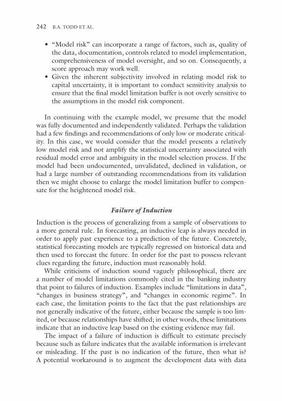
• “Model risk” can incorporate a range of factors, such as, quality of the data, documentation, controls related to model implementation, comprehensiveness of model oversight, and so on. Consequently, a score approach may work well.

• Given the inherent subjectivity involved in relating model risk to capital uncertainty, it is important to conduct sensitivity analysis to ensure that the final model limitation buffer is not overly sensitive to the assumptions in the model risk component.

In continuing with the example model, we presume that the model was fully documented and independently validated. Perhaps the validation had a few findings and recommendations of only low or moderate critical-ity. In this case, we would consider that the model presents a relatively low model risk and not amplify the statistical uncertainty associated with residual model error and ambiguity in the model selection process. If the model had been undocumented, unvalidated, declined in validation, or had a large number of outstanding recommendations from its validation then we might choose to enlarge the model limitation buffer to compen-sate for the heightened model risk.

Failure of Induction

Induction is the process of generalizing from a sample of observations to a more general rule. In forecasting, an inductive leap is always needed in order to apply past experience to a prediction of the future. Concretely, statistical forecasting models are typically regressed on historical data and then used to forecast the future. In order for the past to possess relevant clues regarding the future, induction must reasonably hold.

While criticisms of induction sound vaguely philosophical, there are a number of model limitations commonly cited in the banking industry that point to failures of induction. Examples include “limitations in data”, “changes in business strategy”, and “changes in economic regime”. In each case, the limitation points to the fact that the past relationships are not generally indicative of the future, either because the sample is too lim-ited, or because relationships have shifted; in other words, these limitations indicate that an inductive leap based on the existing evidence may fail.

The impact of a failure of induction is difficult to estimate precisely because such as failure indicates that the available information is irrelevant or misleading. If the past is no indication of the future, then what is? A potential workaround is to augment the development data with data


that is believed to be representative of the forecast. Alternatively, theoreti-cal or business considerations may help to constrain the range of possible forecasts. In any case, because inductive failures lack empirical foundation, these are amongst the most difficult and ambiguous model limitations to address. Consequently, failures of induction may need to be handled via management overlays. These can be any modifications made in order “to capture a particular risk or compensate for a known [model] limitation” [1]. However, in the context of well-developed models, management overlays are applied most effectively to augment model forecasts to better accommodate relevant strategic and business changes.

The relationships between the model limitations buffer and the manage-ment overlay process will be different at different banks. However, given that the model limitation buffer and the overlay process are both concerned with addressing model limitations, some coordination between the model limitation buffer and the management overlay process is needed to prevent either gaps or “double counting”. One potential way to divide responsibili-ties is to consider the model limitation buffer to be concerned with limita-tions that affect all models, namely, residual model error, ambiguity in the model selection process, and model risk. This would leave to the manage-ment overlay process the more idiosyncratic issues associated with particular risks or changes to the business. To some extent, this separation places most of the burden of accounting for uncertainty with the model limitation buffer and most of the burden of correcting potential bias with the management overlay process. However, given the broad involvement of the management and lines of business in the overlay process, it is likely that some overlays will be made to account for uncertainties that are already addressed by the model limitation buffer (e.g. overlays for “conservatism” in the face of uncertainty). In order to avoid “double counting”, it might be appropriate to reduce the model limitation buffer by any model overlays made for the purpose of “conservatism”.

Taking our quarterly bond issuance revenue as an example, a failure of induction might occur if the portfolio has recently become more concen-trated in the oil industry. In this case, the quarterly revenue going forward might cease to depend on market volatility and be more dependent on oil prices. However, since the presumed relationship exists only going for-ward, there are no historical data with which to estimate the sensitivity between the bank’s quarterly revenue and oil prices. In this case, it might be appropriate to augment the development data with publically available industry data. Because addressing this limitation requires knowledge of the business, this limitation may best be handled by a management overlay.


rElatIng IndIvIdual modEl uncErtaIntIEs to a capItal ratIo uncErtaInty

The derivation below describes how individual model errors relate to the errors in the capital ratio change. At the start of the forecast, the bank has qualifying capital Capital0 and risk-weighted assets RWA0. The initial common equity Tier 1 capital ratio, CET10 is then,

CET

Capital

RWA10

0

0

= .

(1)

During the 9Q forecast, the bank has a 9Q cumulative net revenue, Net Revenue, the value of the bank’s qualifying securities change over 9Q by ΔValue, and the bank’s risk-weighted assets change over 9Q by ΔRWA. At the end of 9Q forecast, the capital ratio is,

CET

Capital Net Revenue Value

RWA RWAQ190

0

=+ +

+∆

∆.

(2)

The change in the capital ratio over the 9Q period is,

∆

∆∆

CETCapital Net Revenue Value

RWA RWACETQ1 19

0

00=

+ ++

− .

(3)

For ΔRWA ≪ RWA0, ΔCET19Q can be Taylor expanded to first-order in ΔRWA,

∆∆

∆

CETNet Revenue Value

RWACapital Net Revenue Value

RW

Q190

0

≈+

−+ +

AARWA

02

∆ .

(4)

For the severely adverse scenario Net Revenue + ΔValue will typically reduce capital. We drop Net Revenue + ΔValue from the right-hand term for simplicity noting that this approximation will marginally increase the apparent impact of ΔRWA. At any rate, changes in risk-weighted assets


are not typically a major contributor to the change in capital ratio, so this simplification is not usually material. Making this simplification, we have,

∆∆ ∆

CET CETNet Revenue Value

Capital

RWA

RWAQ1 19 00 0

≈+

−

.

(5)

Equation (5) has an intuitive form. The fractional capital ratio change is the fractional change in capital minus the fractional change in risk weighted assets. Net Revenue includes taxes which, in turn, depending on other components of Net Revenue and ΔValue. For revenue and equity losses experienced under a severely adverse scenario the taxes likely partially offset the loss. In a Federal Reserve Bank of New York (FRBNY) Staff Report, “Assessing Financial Stability: The Capital and Loss Assessment under Stress Scenarios (CLASS) Model”, tax was approximated as 35% of Pre − tax Net Revenue[6]. If this simplified tax treatment is acceptable, the capital ratio change can be written,

∆∆ ∆

CET CETPre tax Net Revenue Value

Capital

RWA

RWAQ1 1 0 659 00

= ×− +

−.00

.

(6)

For more sophisticated accounting of taxes, the capital contributions must be calculated on a pre-tax basis and a detailed tax calculation car-ried out. Equation (6) shows that ΔCET19Q is linear in forecasted Pre − tax Net Revenue, ΔValue, and ΔRWA. Consequently, it is easy to show that the error in the capital ratio change, δCET19Q has the same form as Eq. (6) where each of the forecasted quantities:Pre − tax Net Revenue, ΔValue, and ΔRWA is replaced with the error in that forecast:δPre − tax Net Revenue, δValue, and δRWA. This gives,

δ

δ δ δCET CET

Pre tax Net Revenue Value

Capital

RWA

RWQ1 1 0 659 00

= ×− +

−.AA0

.

(7)

Equation (7) is the basic equation for relating errors in model out-put to errors in the capital ratio; model output is aggregated up to the smallest set of models that can produce a component of Pre − tax Net Revenue, ΔValue, ΔRWA, or any combination thereof. The errors in those


components can then be substituted into Eq. (7) to obtain one instance of the capital ratio error for the model/set of models. Errors can arise from residual model error, ambiguities in the model selection, shortcom-ings in model risk management, and/or failures of induction. A distribu-tion of δCET19Q produced in this manner represents the distribution of errors in the capital ratio arising from a particular model/set of models. The uncertainty in the capital ratio would then be given by analyzing the distribution of capital ratio errors; in the simplest case, the uncertainty in capital ratio could be obtained by evaluating the distribution of capital ratio errors at a given confidence interval. The confidence interval chosen should be consistent with a bank’s model risk appetite.

aggrEgatIng IndIvIdual modEl lImItatIon BuffErs Into an ovErall modEl lImItatIons BuffEr

Throughout this chapter we have focused primarily on approaches for estimating the capital ratio uncertainty for individual models. In order to calculate the impact on a bank’s overall capital ratio, it is necessary to combine the individual model limitation buffers into an overall model limitation buffer for the bank.

While the capital change is just the sum of the individual revenue and equity changes that occur over the forecast horizon, the uncertainty in the capital change is not necessarily the sum of the individual revenue and equity change uncertainties; precisely how the individual uncertainties relate to the total capital uncertainty depends on the correlations in uncer-tainties between different components of the capital change.

The most rigorous way to combine the individual model uncer-tainties is to estimate the correlations between model errors for all models contributing to the model limitation buffer and then propa-gate the uncertainties using the model error covariance matrix. Let δ δ δ δCET CET CET CETQ Q Q Q N1 1 1 19 9 1 9 2 9

� ��= { }, , ,, , , represent the column

vector of the capital ratio uncertainty for the N models used to forecast the capital ratio change. Let

C represent the covariance matrix describing the correlations between the forecast errors of each of the models. Then, the overall model limitation buffer accounting for uncertainty in the total capital ratio change is given by,


Model Limitation Buffer CET C CETQ

T

Q= × ×δ δ1 19 9

� �� .

(8)

The difficult aspect of implementing Eq. (8) is obtaining the covariance matrix,

C . Correlations in the residual model errors can be estimated rela-tively easily by analyzing the time-correlations between dynamic backtests of different models, similar to those shown in Fig. 2b. Describing the correlations associated with ambiguity in model selection would require analyzing whether certain assumptions are common to multiple models, possibly via sensitivity analysis. Further discussion of the covariance matrix is beyond the scope of this chapter.

However, for models that are not overly complex, detailed estimation of the covariance matrix may not be necessary. If the model errors were com-pletely independent, then the square of the total uncertainty would be equal to the sum of the squares of the individual uncertainties. However, as the stress scenarios are, in fact, designed to cause simultaneous stress to many different areas of the bank’s business, the assumption that model errors are uncorrelated may not be prudent. Indeed, if a bank, for instance, experi-enced heavy credit losses across its balance sheet during the 2008–2009 recession, then it is likely that model errors would be highly correlated. In the limit of perfectly correlated model errors (i.e. all models perform poorly at the same time), the total capital ratio uncertainty would be equal to the sum of the individual model error uncertainties,

Model Limitation Buffer CET CET CETQ Q Q N= + + +δ δ δ1 1 19 1 9 2 9, , ,, .

(9)

The assumption of perfect correlations is the most conservative possible assumption for aggregating individual errors as it assumes no diversifica-tion benefit, not even the diversification of having some independence between portfolios. For simple stress testing models and portfolios that are not strongly hedged, this may be a pragmatic and conservative approach. However, for highly granular models, the assumption of perfect correla-tions in model errors may produce very large model limitation buffers. In this case, it will likely be necessary to make use of the correlation matrix.


accountIng for lEss-matErIal modEls In thE Bottom-up approach

A disadvantage of the bottom-up approach to estimating the model limi-tation buffer is that a bank’s inventory of stress testing models is typi-cally quite large. Moreover, the impact of the less material models may be small-to-inestimable. Consequently, it may be necessary or appropriate to use the bottom-up approach only for the material models and then apply a top-down buffer to the less material models.

In order to take this hybrid approach, it will be necessary to estimate the materiality of each model in terms of its contribution to the overall capital ratio change uncertainty. It is clear that no direct measure of a model’s impact on capital ratio uncertainty will be available since it is the goal of the model limitation buffer itself to measure capital ratio uncer-tainty. Consequently, in order to take a hybrid approach, it is necessary to identify reasonable proxies for model uncertainty.

There are number of potential choices for estimating a model or port-folio’s contribution to the capital ratio uncertainty. One approach is to use historical revenue volatility as a proxy; that is, all other things being equal, volatile quantities are more difficult to predict than less volatile quantities, making volatility a reasonable proxy for uncertainty. Prior to estimating the volatility, it may be necessary to de-trend or seasonally adjust histori-cal revenue. Alternatively, it might be appropriate to use the predicted revenue change between base and stress scenarios as a proxy for forecast uncertainty; that is, all other things being equal, quantities that are sensi-tive to macroeconomic factors are more difficult to predict than quantities that are insensitive to macroeconomic factors. Finally, a bank may already have measures of model materiality as part of its broader risk identification efforts. To the extent that these measures can reasonably reflect change in capital under stress, they might be useful in ranking model materiality and estimating the cumulative impact of less material models that are not included in the bottom-up component of a model limitation buffer.

rEfErEncEs

1. Board of Governors of the Federal Reserve System. (December 2015). SR 15-19 Attachment, Federal Reserve Supervisory Assessment of Capital Planning and Positions for Large and Noncomplex Firms.


2. PwC. (2015). Model Uncertainty/Model Risk Quantification Industry Survey. PwC Survey Results.

3. Board of Governors of the Federal Reserve System. (October 2014). CCAR 2015 Summary Instructions and Guidance, Board of Governors of the Federal Reserve System.

4. Brockwell, P.J. and Davis, R.A. (2002). Introduction to Time Series and Forecasting, Springer, 2002, Second Edition.

5. Board of Governors of the Federal Reserve System and Office of the Comptroller of the Currency. (April 2011). SR Letter 11-7 Attachment, Supervisory Guidance on Model Risk Management.

6. Hirtle, B., Kovner, A., Vickery, J., and Bhanot, .M (2014). “Assessing Financial Stability: Capital and Loss Assessment Under Stress Scenario (CLASS) Model”, Staff Report No. 663, October 2014.


Modern Risk Management Tools


Quantitative Risk Management Tools for Practitioners

Roy E. DeMeo

R.E. DeMeo (*) Wells Fargo & Co., 12404 Elkhorn Drive, Charlotte, NC 28278, USA


IntroductIon to Value at rIsk

We will start by defining the most basic measure of the risk of large losses, namely value at risk, or VaR. VaR, is briefly speaking, a measure of how much money a bank or other financial firm can lose on its positions in a fixed period, such as one day, ten days, or one year in a “worst case” (e.g. worst 1%) scenario.

Basic Assumptions The environment we work in is always defined by (Ω, F, P), a triple consisting of, respectively, (1) a probability space, or set of scenarios, (2) a σ-field or set of measurable sets, and finally (3) a probability measure on that σ-field.

Definition 1.1 Let V(t) be the value of your portfolio on a date t in the future. Let P be the real-world (NOT risk-neutral) measure, and let Δt > 0 be a fixed time horizon. Let t = 0 denote today. Then

254

VaR p P V V t p( ) = ( ) − ( ) ≥{ } ≤ −( )min( | . 0 1∆

(1)

For VaR as specified by Basel II, p = 0.99.

This measure of risk of loss has some drawbacks:

1. VaR tells you where the beginning of the tail is, and does not mea-sure the overall tail impact on risk (expected shortfall, which will be covered later, is a stronger attempt to do that).

2. VaR does not consider liquidity—a one-day VaR only considers changes in mid market price, and does not consider inability to sell at that price in extreme conditions. The concept of liquidity horizon, the minimum time it takes to unwind the position and get some-thing close to the market value, tries to address this issue. For this reason we also will discuss ten-day VaR, which is part of Basel II capital requirements and accounts for the fact that it might take ten days, rather than one day, to unload a position.

3. Because of illiquidity and because of potential model risk on the future realizations of portfolios, it is inaccurate, strictly speaking, to think of VaR as saying that the bank will not lose “this much” tomorrow with a 99% probability. It will be much worse if you try to actually unload the position, and your models may be off.

4. VaR does not always behave well when aggregating portfolios, meaning that the sum of VaRs for two portfolios is sometimes less than the VaR for the aggregate portfolio. It is quite possible for two portfolios to each have a VaR of less than $500,000, but the aggre-gate portfolio to have a VaR of greater than $1,000,000. In other words, the diversification principle can fail in the case of VaR.

Example 1.2 Suppose we have a single unhedged stock position that fol-lows a real-world lognormal process

dSS

dt dw= +µ σ .

Then for a given value of p, we can compute VaR by solving

R.E. DEMEO

QUANTITATIVE RISK MANAGEMENT TOOLS FOR PRACTITIONERS 255

P S S pt∆ < −( ) ≤ −0 1 .

This translates in this case to

NS S t t

tp

ln / /0 02 2

1−( )( ) − +

≤ −

µ σ

σ

∆

∆

≥ −

− + −( )−

S et t N p t

0

12

11

2 1µ σ σ∆ ∆ ∆

VaR S et t N p t

= −

− + −( )−

0

12

11

2 1µ σ σ∆ ∆ ∆.

In this notation, we are using the cumulative normal probability distribution

N x e dt

tx( ) = −

∞∫12

2

2

π.

In particular, if S = 100, μ = 0.08, σ = 0.25, the one-day 99% VaR works out to $3.58, and the ten-day 99% VaR is about $10.77.

Example 1.3: VaR Based on Factor Model (Variance-Covariance Estimate) Suppose that there is a total of d risk factors X1 , … , Xd for a position with value V and their shifts ΔXi are jointly normal with

E Xi i∆( ) = µ

var ∆Xi i( ) =σ 2

corr X Xi j ij∆ ∆,( ) = ρ .

Let the first order sensitivities to the risk factors be

δ i

i

VX

=∂∂

.

256

Then, up to first order, the one-period loss is

L V Xi

d

i i= − ≈ − =∆ ∆1∑ δ

and L has a normal distribution with mean M and standard deviation Σ, where

M i

d

i i= − =1∑ δ µ

Σ2

12 2 2= += <i

d

i i i j i j ij i j∑ ∑δ σ δ δ ρ σ σ .

It then follows, using an analysis similar to that of Example 1.2, that

VaRp M N p= + −Σ 1 .

Note that this approximation is exact if the position value V is linear in all the risk factors, as in the case of a portfolio of stocks. However, a port-folio of derivatives has a non-linear dependence on all the risk factors, and its VaR will be discussed later in the upcoming analysis.

Overall, there are three basic calculation methods for VaR and each of them is discussed in greater length separately in the subsequent discussion:

1. Analytical formulas or approximations—rarely possible unless the underlying pricing models are extremely simple.

2. Historical simulation—last N one- or ten-business-day interval market changes are applied to current conditions, and we take the loss corresponding to the 99th percentile. The Feds allow N as low as 251 (one year), with the second worst loss chosen as the VaR. Some banks use two or three years’ worth of data, with the VaR being the fifth or seventh worst loss in those cases.

3. Monte Carlo model—Create a parametric model for the next peri-od’s moves based on current pricing models and sufficient historical data, simulate N times, take the least of worst 1% of losses.

We have just given examples of (1). We will now describe (2).

R.E. DEMEO


Value at rIsk: HIstorIcal sImulatIon and loss calculatIon

We assume that the firm has trading positions with values Vj , j = 1, …, M, and that each position has risk factors X X Xj j n jj1 2, , ,…{ } chosen pri-marily from market observable inputs, rather than from underlying cal-ibrated parameters (see section “Market Data Inputs Versus Calibrated Parameters” below for more discussion of this topic). Furthermore, each risk factor has historical time series Xi , j(t) and one-day shifts ΔXi , j , t = Xi , j(t) − Xi , j(t − 1) (absolute) or ΔXi , j , t = (Xi , j(t) − Xi , j(t − 1))Xi , j(0)/ Xi , j(t − 1) (relative).

Full Revaluation

Now for each time t, and each position indexed by j, define

∆ ∆ ∆V t V X X X X

X

j j j t n j n j t

j

j j( ) ( ) , , , , ( )

( ), ,

, , , , , ,

,

= + … +( )−

1 1

1

0 0

0V ……( ), , ( ),Xn jj0

(2)

Then the total P&L across all positions is

∆ ∆V t V tj

M

j( ) = ( )=1∑ .

(3)

Finally, sort all N losses, (−ΔV(t))'s, one for each business day over the N-day historical period ending yesterday, from high to low, and take the one most closely corresponding to the 99th percentile. If using N=251, as federal regulators allow, take the second worst loss. Note that this is not really the 99th percentile of losses, really it is closer to the 99.2 percentile, but the regulators do not allow interpolating between the second and third worst P&L.

258

Delta-Gamma Approximation

The delta-gamma approximation to the daily historical P&L for a posi-tion is

∆ ∆ ∆ ∆V t Vt

tVX

XVX

Xj i

n j

i ji j t

j

i ji j t

j( ) ≈ ∂∂

+∂

∂+

∂

∂

=1

2

221

2∑

,, ,

,, ,

+∂

∂ ∂<i kj

i j k ji j t k j t

VX X

X X∑2

, ,, , , , .∆ ∆

(4)

This is just the second order Taylor series approximation to (2), in con-trast to the first order approximation of Example 1.3.

The purpose of this approximation is to potentially save time; the number of position values we need to compute for (2) is M(N+1), which can be quite large. In practice, when computing (4) it is common to leave out the cross gamma terms, which are usually (but not always) relatively small, and also the time derivative (theta) term at the begin-ning, to arrive at

∆ ∆ ∆V tVX

XVX

Xj i

n j

i ji j t

j

i ji j t

j( ) ≈∂

∂+

∂

∂

=1

2

221

2∑

,, ,

,, , .

(5)

The most common way to calculate these “Greeks” is to use central finite differences, with a bump size h, as in

∂∂VX

V X X h X V Xj

i j

j j i j n j j jj

,

, , , ,, , , , , , , , , , , , , , , , , , , ,=

… + …( ) − …1 1 ,, , , , , , , , , , , ,

, , , , , , , ,

, ,

,

, ,

X h X

h

VX

V X X

i j n j

j

i j

j j i

j− …( )

=…

2

2

2

1∂∂

jj j j j j i j nh X V V X X h Xnj j+ …( ) − + … − …, , , , , , , , , , , , , , , , , , , , , , , ,, , ,2 1 ,,

.j

h( )

2

(6)

For certain risk factors, such as stock price, it is common to use relative bump sizes, which means substituting hXi , j for h. Observe that the total number of prices you need to calculate is now

R.E. DEMEO


#NPVs M nj

Mj= + ∑ =2 1 .

This is usually a much smaller number than M(N + 1).The bump size h can affect the accuracy of the delta-gamma approxima-

tion, and we argue that we can achieve the smallest mean-squared error versus full revaluation by setting

h var X mean X absolute

h varXX

i j i j ij

i ji j

i j

, ,

,,

,

( )≈ ( ) + ( )( )

≈

∆ ∆

∆

2

+

meanXX

relativei j

i j

∆ ,

,

( ).2

To see this, consider the case of a single risk factor, and the absolute case. In that case we want

V X X V X+( ) − ( )∆

to be as close as possible, on average, to

V X h V X hh

XV X h P X V X h

hX

+( ) − −( )+

+( ) − ( ) + −( )2

12

22

2∆ ∆ .

By expanding the Taylor series on both sides, we see that we want

′ ′′ ′′′

′

+ + + ≈

+

V X X V X X V X X V X X

V X X

( ) ( ) ( ) ( )

( )

∆ ∆ ∆ ∆

∆

12

16

124

12

2 3 4′′′′

′′′ ′′′+ +V X X V X h X V X h X( ) ( ) ( )∆ ∆ ∆2 2 2 216

124

′′′′

From the last two terms we see that we really want

h X2 2≈ ∆

260

on average, which implies the result stated above. The argument is very similar for two or more risk factors, given that we do not include the cross gammas in the approximation.

Market Data Inputs Versus Calibrated Parameters

It is worth mentioning that the risk drivers for VaR, or the values Xi are typically market inputs, for example, spot, at-the-money volatility, some sort of volatility skew measure, and interest rates, rather than underlying model parameters. Full revaluation requires recalibration of the underlying parameters for every historical shift. Delta-gamma approximation requires inverting a Jacobian matrix. More precisely, suppose that

X X G Y Yj n j j n jj j1 1, , , , ., , , ,…( ) = …( )

Then

∂

∂…

∂

∂

=∂

∂…

∂

∂

−V

XVX

JVY

VY

j

j

j

n j

T

j

j

j

n jj j1

1

1, , , ,

, , , ,

T

In this notation, J an nj × nj matrix such that the (i, k) entry is

J

XYi k

i

k, .=

∂∂

Second derivatives are messier but can be worked out.To illustrate it, we consider a model for credit default swaps out to two

years which depend on a one-year credit spread s1 and a two-year credit spread s2. Suppose for simplicity that discount rates are 0, and the recovery rate is a constant R, and that coupons are paid with accrued interest up to the time of default. Then we can evaluate any credit spread out to two

R.E. DEMEO


years if we know the underlying instantaneous piecewise-constant hazard rate λ1 for times t ∈ [0, 1], and the forward instantaneous hazard rate λ2 for times t ∈ [1, 2].

By assuming that a credit spread with tenors one or two years with par coupons s1 , s2, respectively, have a net present value of 0, we can work out the following simple relationships between (s1, s2) and the hazard rates (λ1, λ2):

s R1 11= −( )λ

s

R e

e e e21 2

2 2 1 1

1 1 1 2

1 1 1 2=

−( ) −( )− + −

− −

− − − −

λ λ

λ λ λ λ

λ λ

λ λ λ λ .

Then the Jacobian matrix, as discussed above, will have the following entries, with the first two being on the first row and the last two being on the last row:

∂∂

= −s R1

1

1λ

∂∂

=s12

0λ

∂∂λ

λ λ λ λ λ λλ λ λ λ λ λ λ

s R

e e e e

2

1

22

22

1 22

22

22 2

1

1 2 1 2 1 1

= −

− + − +− − − − − − −

( )

22 1

1 1 2

1 1 1

1 22

12

2 2 1

2 2 1 1

−+ −

− + −

−

− − −

− − − −

λ λλ λ λ λ

λ λ λ λ

λ

λ λ λ

λ λ λ

ee e

e e e λλ22( )

∂∂λ

λ λ λ λ λ λλ

λ λ λ λ λ λ

s R

e e ee2

2

12

1 22

12

2 12

12

1

1 2 1 2 1 2

= −

+ − −−

− − − − − −

−

( )22

1 22 2

1 22 2

12 2

2 2

1 2 1 2 1 2 1 2

1

λ λ λ λ λ λ λ λ

λ

λ λ λ λ λ

λ λ λ

− − − − − − −

−

− + +

− +

e e e

e 11 1

21 1 2e e− − −−( )λ λ λλ

.

Then, rather than bumping the credit spreads and backing out the haz-ard curve each time, we can instead bump the hazard rates and use the Jacobian formula shown above.

262

Grid Approximation for Risk Factors

Another commonly used method of accounting for a risk factor is to replace the delta-gamma approximation for that risk factor with a one- dimensional grid. Clearly higher-dimensional grids are possible as well, but the number of NPVs to calculate rapidly grows with the dimension. It is common practice among the banks to combine a grid approximation for some risk factors with delta-gamma approximations for other risk factors.

If we wish to create a grid for the first risk factor, we create a symmetric array of the form (h−m , h−m + 1 , … , h−1 , 0 , h1 , … , hm), with h−k = − hk, and compute NPVs of the form

V X h X X V X X V X h Xj m n j n j mj j1 2 1 1 2+ …( ) … …( ) … +− ,,, ,,, ,,, ,, ,, ,,, ,, , , , ,,, ,,,…( )Xnj

for an absolute grid and

V X h X X V X X V X hj n n j n j nj j1 2 1 11 1+( ) …( ) … …( ) … +(− ,,, ,,, ,,, ,, ,,, , , , ( )) …, , , )X Xnj2

for a relative grid. In either case we might refer to these 2m + 1 NPVs as

V V V V V V Vm m m1 1 1 1 1 1 0 1 1 1, , , , , ,, , , , , , , .− − + −… = …

More generally, if we were using the kth risk factor, we would refer to these NPVs as

V V V V V V Vk m k m k k k k m, , , , , ,, , , , , , , .− − + −… = …1 1 0 1

Relative grids are more common because the major risk factors for which banks employ a grid are typically spot price or volatility, which are always positive. For a relative grid in the risk factor X1, suppose that

∆XX

h hk k1

111 01= −( ) + ∈[ ]+ρ ρ ρ, .,

R.E. DEMEO


Then we set

∆V V V Vk k1 1 1 11= −( ) + −+ρ ρ, , .

This is the P&L contribution from the first risk factor. Though one- dimensional grid approximations still leave out the cross term risk, they are often more accurate than delta-gamma approximations for larger shifts since the latter is a parabola in the risk factor shifts. This grows much more rapidly than most pricing functions, in terms of spot, volatility, or interest rate shifts. For example, a vanilla call option approaches linearity as spot increases, and approaches zero as spot decreases. If we were computing VaR for an at-the-money call with strike equal to spot, the parabolic func-tion given by the delta-gamma approximation would become quite large as spot approached zero, rather than going to zero, and as spot increased in the other direction, the parabolic function would grow much faster than a function approaching a straight line.

One Day Versus Ten Days

Federal regulators require that banks calculate VaR with both a one-day and ten-day time horizon. For ten-day risk factor shifts, we let

∆X X t X t absolutei j t i j i j, , , ,= ( ) − −( ) ( )10

or

∆XX t X t X

X trelativei j t

i j i j i j

i j, ,

, , ,

,

.=( ) − −( )( ) ( )

−( ) ( )10 0

10

If N is the total number of historical returns we use, the returns begin on consecutive days, and overlap, meaning that we require N + 9 days of data. If daily returns are i.i.d. (independent and identically distributed), then

10 10 1− = −( )dayVaR dayVaR .

264

In the case of an organization with limited computing power, the Feds may sometimes accept this approximation for ten-day VaR under certain conditions. See Section 5 of [1].

Stressed VaR Versus General VaR

In the case of stressed VaR, the calculation is exactly the same as for gen-eral VaR, except that the historical shifts are derived from a “stressful” period in the past, where the risk factors were likely to be much more volatile. In general, if we want N k-day intervals, we choose a set of busi-ness days in the past of the form

T T T N k, , , .+ … + + −1 1

Then for a position with value V X Xj j j n j, , ,1, ,…( ) we would calculate the loss

L V X X V X X X Xj j j n j j j t j n jj j= …( ) − + … +, , , , , , ,( ), , ( ) ( ) , , ( )1 1 10 0 0 0∆ ∆ nn tj ,( )

t T T T N= + … + −, , ,1 1

∆X X t k X t absolutej i t j i j i, , , , ( ) ( )= +( ) −

∆XX t k X t

X tX relativej i t

j i j i

j ij i, ,

, ,

,,

( )( )

( )( ).=+( ) −

0

The argument zero as usual stands for today or the most recent close date, but the difference here is that the last close date does not coincide with the last day of the history, namely T + N + k − 1, as it does for general VaR. Typically for regulatory purposes k = 10, and it is standard practice to choose the historical period so as to maximize the resulting total VaR for the bank’s entire trading book subject to regulation. One example of a very stressful period is the one-year period from April 2008 to April 2009. Once again, the Feds allow as little as a year’s worth of starting times, that is N = 251. For details on this, see [1], Sections 4 and 5.

R.E. DEMEO


Value at Risk: Backtesting Versus Actual P&L

The purpose of backtesting is to determine whether a particular VaR model can be considered a good or reasonable measure of risk. More precisely, a VaR model is considered to be a good measure of risk if the actual loss in a particular one-day or ten-day period does not exceed the VaR for the beginning of that period, more often than with probability p. Generally, if we are using a VaR calculation with p = 0.99, we should not see more than around two to three breaches, or exceptions, per year. To formalize this con-cept, we note that, using the real-world probability measure P, we have

P exceptions m nn k k

p pk m

n n k k# !! !

.≥( ) =−( )

−( )=−∑ 1

If you experience m exceptions over a period of m business days and this probability is less than 5% it is considered unlikely that the probability of an exception is 1−p. If m is too high, the VaR model is not adequately capturing the risk, and if m is too low (e.g. you never see an exception year after year), then you are too conservative. Generally speaking, since it results in an overestimate of regulatory capital, the federal regulators are never concerned if a bank is too conservative.

Here is an example in which p = 0.99, and n = 252:

Number of exceptions (m) P(#exceptions = m) P(#exceptions >= m)

0 7.94% 100.00%1 20.22% 92.06%2 25.64% 71.83%3 21.58% 46.20%4 13.57% 24.62%5 6.80% 11.05%6 2.83% 4.25%7 1.00% 1.43%8 0.31% 0.42%9 0.09% 0.11%

10 0.02% 0.03%

Note that the Feds will start to have serious doubts about the VaR model if there are six or more exceptions in a year, and in fact, there are increasing capital requirements for four or more.

266

Value at rIsk: monte carlo sImulatIon

The last approach for computing the VaR is to through a Monte Carlo simulation engine. Monte Carlo simulation works by creating a parametric model for the historical distribution, and simulating it a number of times N which is typically much larger than the number of days covered by the history. This removes the primary limitation of historical simulation, that is, if you are only going back a year, you only have about 250 business days to work with. By contrast, Monte Carlo simulation enables us to use 10000, 50000 or even a million scenarios, if there is enough hardware available. Therefore, the limitation of Monte Carlo is in the quality of the model and computation time, not in the number of scenarios.

Monte Carlo Basics

We assume that there are d risk factors affecting your position, and we denote these by X1 , … , Xd. We assume that the one-period changes in these risk factors have a cumulative probability distribution

F x x P X x X xd d d1 1 1, , , ,…( ) = ≤ … ≤( )∆ ∆ .

As usual, we assume that the probability measure P is the real-world measure. We simulate this distribution N times, and denote a particular scenario out of N by ω. Now compute

L V X X V X X X Xd d dω ω ω= …( ) − + … +( )1 1 1, , , ,∆ ∆, , .

Sort the losses in ascending order, and choose the loss at the correct percentile, in other words if p=0.99 and N=10000, then choose the 9900th loss.

We assume for this exposition that the actual historical risk factors shifts, or time series, denoted by (ΔX1, t, …, ΔXd , t), t = T , T + 1, … , T + n, are independent and identically distributed (i.i.d.). The model we create is known as an unconditional model. A conditional model is based on a time series in which we assume that the distribution of (ΔX1 , t, … , ΔXd , t) can depend on the values of (ΔX1 , s, … , ΔXd , s) for s < t. There is a great deal of literature on conditional models, (see [1]) but these are beyond the scope of this brief overview.

R.E. DEMEO


Monte Carlo VaR for Beginners

The simplest Monte Carlo algorithm involves assuming that the distribu-tion of the risk factor shifts (ΔX1, … , ΔXd) is joint normal. Specifically, we express a multivariate normal distribution in vector form as

X AZ= +µ

Z Z Z iid Nk

T= …( ) ( )1 0 1, , ,, , ~

A d k matrix= ×

µ µ µ= …( )1, , d

T

This distribution is joint normal with means μ and covariance matrix Σ = A • AT and we write this as

X N~ .µ,Σ( )

To simulate this distribution, we first make use of the

Cholesky Decomposition Suppose that X is d-dimensional with X ~ N(μ, Σ). Suppose, further that Σ has full rank d. Then you can write the covariance matrix as

Σ = A AT• ,

with A being lower triangular (d x d) with positive diagonal entries.One then follows the following four steps for a 99% VaR with 10000

scenarios:

1. Compute the historical means over the last year, or several years, denoted by μi and their historical standard variances, denoted by σ i

2 . 2. Compute the historical covariances σi , j, rounding out the rest of

covariance matrix, denoted by Σ. 3. Use Cholesky decomposition to simulate (ΔX1, … , ΔXd) as multi-

variate Normal N((μ1, … , μd), Σ) 10000 times and each time

268

compute V(X1, … , Xd) − V(X1 + ΔX1, … , Xd + ΔXd) by delta/gamma approximation, grids or full revaluation, if you have enough machines.

4. Choose the 100th worst of these losses for VaR and take the average of the 100 worst for ES, for p = 0.99.

Evidently, the joint distribution of changes of n risk factors for a typical asset class would not be multivariate normal—they usually have fat tails—in other words the risk of an extreme move is far greater than what would be implied by a normal distribution. In fact, this “beginner” method would never pass muster with the regulators. We will now look at methods of creating more realistic models for Monte Carlo VaR.

Some Important Basic Statistics

Theoretical Skewness, Kurtosis Let σ be the standard deviation of a probability distribution of a random variable X, and let μ be the mean. Then skewness and kurtosis are respectively,

β

µ

σ=

−( )( )E X 3

3

κ

µσ

=−( )E X( 4

4

If X is a normal random variable, β = 0 and κ = 3.

Sample Mean and Covariance Matrix Suppose we have n samples of the d-dimensional random variable X, namely

X Xn1, , .⊃

Then the sample mean and the covariance matrix are:

R.E. DEMEO


X n Xi

n

i= −=

11∑

S

nX X X Xi

n

i iT

= −( ) −( )=

11∑

It is well known that using 1/(n − 1) instead of 1/n makes the covari-ance estimator unbiased.

Sample Skewness and Kurtosis Let X1 , … , Xn be n samples of the sca-lar random variable X, and let X n X Xn= +…+( )−1

1 be the sample mean. Now let

β Xn X X

n X X

i

n

i

i

n

i

( ) =−( )−( )( )

−=

−=

11

3

11

2 3 2

∑

∑/

κ Xn X X

n X X

i

n

i

i

n

i

( ) =−( )−( )( )

−=

−=

11

4

11

2 2

∑

∑

Why do skew and kurtosis matter? Kurtosis is a measure of tail risk. If κ(X) > 3 that means that the tails are “fat”, and computing VaR using a normal distribution with the same mean and variance will likely understate the risk. Stock and foreign exchange price returns are typically “leptokur-tic” (fat-tailed). Skew is a measure of asymmetry about the mean. Stock price returns are negatively skewed, with big losses more likely than big gains. Our next goal is to go beyond “beginner” and create joint distri-butions with the right covariance and whose marginal distributions are skewed and fat-tailed.

270

Some Important Tests

As mentioned in section “Monte Carlo VaR for Beginners”, the Monte Carlo simulation for a “beginner” is to employ a joint normal distribution. A natural question is: Are the marginal distributions normal? The Jarque- Bera test indicates whether a one-dimensional distribution is likely to be normal. By using the sample kurtosis and skew above, we define

T n= + −( )

16

14

32 2β κ .

As the sample size n gets larger, if the distribution is normal, T will approach a chi-squared distribution with two degrees of freedom, which turns out to be exponential:

Pr / /T t e du e

t

u t≤( ) ≈ = −− −∫0

2 212 1

for large values of n.

How Well Does Your Model Fit the Data? Let X1 , X2 , … , Xn be n samples of an unknown d-dimensional distribution, and suppose we want to fit a distribution with a density of the form

f ; a , ,amX a a( ) = …( ), 1

is a set of parameters. Since we assume that the samples are independent, we want to maximize, over all possible choices of the parameters, the log of the likelihood of seeing these samples, namely

Λ = …( )( ) = …( )( )= =∏ln ln .i

n

i m i

n

i mf X a a f X a a1 1 1 1; , , ; , ,∑

We call this the maximum log likelihood calculation.

R.E. DEMEO


A Simple Type of Fat-Tailed Distribution

Let

µ µ µ= …( )1, , d

T

W isanr v≥ 0 . .

Z Z Z N I k nk

Tk k= …( ) ( ) ≤1 0, , ,~ ,

A d kε ×

Next we require that W be independent of the Z’s. Then the random vector

X W AZ= +µ

is said to be a normal mixture model. The simplest example of this sort of model would be the one-dimensional case

X WZ= +µ .

Observe that, for this one-dimensional case,

E X( ) = µ

Var X E W( ) = ( )

β X( ) = 0

κ XE W

E W

Var W

E W( ) =

( )( )( )

= +( )

( )

3 3 12

2 2 .

In the special case where E(W) = 1, we get

κ X Var W( ) = + ( )( )3 1 .

272

It follows immediately that the marginal distributions of a normal mix-ture always have fat tails. We can then consider a two-dimensional exam-ple, expressed as

X WZ1 1 1= +µ

X WZ2 2 2= +µ

with corr(Z1, Z2) = ρ. Then note also that corr(X1,X2)

= ( ) =corr W Z WZ1 2, ρ. This means that we can use normal mixtures to add kurtosis without changing the correlation matrix. Also note that because of the independence of W and Z , cov(X1, X2) = E(W)cov(Z1, Z2), and more generally

cov X E W( ) = ( )Σ.

Note, however, that there is only one kurtosis level.To simulate such a fat-tailed distribution of X, it is enough to generate

instances of the d-dimensional normal distribution Z and also the single scalar random variable W. In the case where W is absolutely continuous with a density function h and cumulative distribution function H, a simple (even though it is not always the most efficient) way to simulate W is to choose a uniform random variable U and set W = H−1(U).

To compute the density of this distribution is straightforward. Note that if D is the domain of W, then

f x f x w h w dw

DX W( ) = ( ) ( )∫ | |

=( )

−−( ) −( )

( )∫

− −

D

n

n

Tw x x

wh w dw

/

/ exp .2

2

1

2 2π

µ µ

Σ

Σ

Special Case: The t-Distribution

To illustrate the aforementioned idea, we focus on only one simple exam-ple of a fat-tailed distribution that we can try to fit to the historical data for d risk factor shifts. Consider the following distribution for W, known as the inverse gamma distribution, or IG(α, β):

R.E. DEMEO


h w e w ww

( ) = ( )>

− − −βα

α β α/

, ,1

0Γ

Γ α α( ) =

∞

− −∫0

1x e dxx

α β> >2 0, .

Then the d-dimensional normal mixture random vector with α βν

= =2

has what is known as the multivariate t distribution with ν degrees of freedom. From the formula in section “A Simple Type of Fat-Tailed Distribution”, it is possible to derive the density in closed form as

f xd x xd

T

( ) =+( )

( )( )+

−( ) −( )

−Γ

Γ Σ

Σ122

12

1ν

ν πν

µ µν/ /

−− +( )ν d / 2

This is a popular fat-tailed distribution for fitting certain common types of risk factor sets, such as portfolios of stocks.

To choose a suitable t-distribution for our data, one simple and intui-tive approach is to match the mean and covariance matrix and choose the parameter ν which yields the maximum log likelihood. First, we express the multivariate t distribution as

X AWZ= +µ .

Here, for notational simplicity, we are using the notation X to refer to risk factor shifts which we would ordinarily refer to as ΔX = (ΔX1, … , ΔXd)T. To match the covariance matrix, let µ µ x − be the sample mean of X, let Σ

be the sample covariance matrix of X, and let Σ = AAT be the covariance of Z . Then we want to have

E W( ) =

−ν

ν 2

cov X( ) =

−ν

ν 2Σ

274

Σ Σ=

−νν2.

The density function now becomes

f xd x

d( ) =

+( )

( ) −

+−

−Γ

Γ

12

22

12

1ν

ν νν

µ

π νΣ

Σ

x T −−

−

−+

µ

ν

ν

2

2d

,

which implies that the log likelihood we want to maximize is now

= ∑+( )

( ) −

+−

=k

N

d

kd X

12

12

22

1lnΓ

Γ Σ

ν

ν πν νν

µ

T

ΣΣ−

−+

−

−

1 2

2

Xk

d

µ

ν

ν

= +( )

−

− −

− −N d N N d N Nln ln ln ln lnΓ Γ

12 2 2

12 2

νν

ν Σ νν −( )2

− − ∑+

+−

−

−

=

−

Nd dX X

k

N k

T

k

2 21

21

1

ln lnπν

µ µ

ν

Σ

.

There are number of simple numerical algorithms which can maximize this expression, and the result will be a distribution with the same means and covariances as your sample, but with the optimally chosen kurtosis for best fit to the data.

R.E. DEMEO


Fitting a Distribution with the E-M Algorithm

Another way to fit a t-distribution, or any other distribution of this type, is with an iterative procedure known as the E-M(expectation-maximization) algorithm. In this case we are not insisting that we match the sample cova-riance matrix exactly first, but as a result we might obtain a better overall fit based on maximum likelihood.

The way to think of the E-M algorithm is that it “seesaws” between estimating the multidimensional parameters Σ, μ and the parameters of the distribution of W. The basic tasks are:

(A) Express the joint density of (X, W) as the product of the density of W and the density of X|W.

(B) Estimate the parameters Σ, μ based on the latest estimates of your W parameters and the known values of the samples Xi , i = 1 , … , n.

(C) Then do maximum log likelihood to get the parameters of W using the density function h but you don’t have the Wi’ s so instead you use expectations of certain functions of the W si

, which in turn

were derived from the latest Σ, μ and the distribution of W|X given those parameters.

(D) Keep doing (A) and (B) until you achieve convergence.

We will now present a more precise, numbered, set of steps for the t-distribution. First note that in the case of the t-distribution, W has only one parameter ν, and by Bayes’ theorem we can express

f

f hfW XX W

X|

| ,=

so that

fW X wx d wdx T x

w| / /exp|( )

( )( ) ( )

= − − − −1

2 2 2

12

2π

µ µν

Σ

Σ

− − −

ν ν ν

ν

/ / /2 2 2 1

12

eww

Γ

276

×( )

+

+−( ) −( )−πν ν

νµ µ

dT

dx x

/ 212

2 2

1Σ Γ

Γ

Σνν

ν

+2 2

d

=+ −( ) −( )

+ −( ) −( )

−+

−ν µ µ ν µ µν

x x x xw

Td

TΣ Σ1 2 2 1

2 2exp

− − −

wdν

2 21.

Thus the conditional distribution of W given X is inverse gamma with parameters α , β, that is, IG(α, β), with

α

ν= +2 2

d ,

β

ν µ µ=

+ −( ) −( )−x xT Σ 1

2.

In addition, the log likelihood of the overall density breaks down as

= ∑ ( ) + ∑ ( )

= =i

n

X W i ii

n

W if X W h W1 1ln ln .| |;, |;, |;, ;µ νΣ

Armed with this important information, we can now give an exact rec-ipe for the algorithm.Step 1 Set

µ µ1[ ] =

Σ Σ1[ ] =

,

the sample means and covariances, and let ν[1] be some “reasonable” first guess for ν. For notational conciseness, let θ[1] = (ν[1], μ[1], Σ[1]). Let k be the iteration counter, and set that equal to one.

R.E. DEMEO


Step 2 Calculate the following:

α

νkk d[ ][ ]

=+2

β ν µ µi

k ki

k T ki

kX X[ ] [ ] [ ] [ ] − [ ]= + −( ) ( ) −( )

12

1Σ

δ θαβ

ik

i ik

k

ik

E W X[ ] − [ ][ ]

[ ]= ( ) =1|; |;

δ δk

i

n

ik

n[ ]

=

[ ]= ∑11

.

Step 3 Let

µ

δ

δk i

n

ik

i

k

X

n+[ ] =

[ ]

[ ]=∑

1 1

Ψ = ∑ −( ) −( )−

=

[ ] +[ ] +[ ]n X Xi

n

ik

ik

ik T

1

1

1 1δ µ µ

ΣΣ Ψ

Ψk

d

d+[ ] =1

1

1

/

/ .

Step 4 Define an intermediate set of parameters θ[k, 2] = (ν[k], μ[k + 1], Σ[k + 1]). Then let

β ν µ µi

k ki

k T ki

kX X,2 1 1 1 112

[ ] [ ] +[ ] +[ ] − +[ ]= + −( ) ( ) −( )

Σ

δ θαβ

ik

i ik

k

ik

E W X, ,,

| ;2 1 22

[ ] − [ ][ ]

[ ]= ( ) =

ξ θ εα ε β

α

ε

ik

i ik

kik

kE W X, ,

,

ln | ;2 2 1

2

1[ ] [ ] −

[ ] [ ]

[ ]= ( ) ≈

−( )( )( )

− Γ

Γ

( )ε small .

278

Step 5 In the equation

∑ ( ) = ∑

− − +

−

= =

−

i

n

ii

n

i ih W W W1 1

1

2 2 2 21ln ln ln ln;ν ν ν ν ν

Γνν2

,

substitute δ ik ,2[ ] for Wi

−1 and ξii ,2[ ] for ln Wi. Now maximize function over

all possible values of ν, to obtain ν[k + 1].

Now let θ[k + 1] = (ν[k + 1], μ[k + 1], Σ[k + 1]), replace k by k+1, go back to Step 2, and repeat Steps 2–5 until you achieve convergence.

This algorithm can be generalized to any multivariate distribution which takes the form of a normal mixture. The only difference might be that if the density h(w) has more than one parameter, then Step 5 will be more complex, and the conditional distribution fW|X(w| x) may be more chal-lenging to work out, but other than that the algorithm would be the same.

Expected Shortfall

Within a few short years, it will no longer be acceptable to regulators for banks to use general and stressed VaR as key risk management tools; they will be required to replace it with a variant known as expected shortfall, or ES for short.

To understand what ES is, think of VaR as a high percentile of the possible losses; ES, on the other hand, is the average of the tail beyond a certain percentile. More rigorously, define

ES E V V t V V tPα α( ) = ( ) − ( ) ( ) − ( ) ≥( )0 0∆ ∆| .

To define α in terms of a percentile, we may write, for some probability p,

α = ( )VaR p .

If a bank uses p = 0.99 for VaR, it is likely to use a somewhat lower probability, such as p = 0.975, for ES, and in fact upcoming federal regu-lations will specify this level (see Section D3 of [2]). Though this risk measure is harder to do backtesting for than VaR, it has one key advantage

R.E. DEMEO


over VaR, that is, it satisfies subadditivity. Precisely, given two portfolios P1 , P2, and P = P1 + P2, then

ES P ES P ES P1 2; ; ;α α α( ) + ( ) ≥ ( ).

As mentioned above, VaR is not guaranteed to satisfy this property, and it is easy to come up with an example. Suppose that on October 1, 2015, you are doing one-year historical VaR, using the second worst loss, and P1 has the two worst losses of $110 and $150 corresponding to historical shifts that occurred on January 14 and May 1. On the other hand, P2 had its two worst losses on the exact same two historical shift days, but those losses were $130 and $100, respectively. Then the aggregate portfolio P must have its worst two losses on those exact days of $240 and $250, giv-ing us a VaR for P of $240. But note that

VaR P1 110( ) = $

VaR P2 100( ) = $ .

Since ES is the average of the tail, it is also considered a better measure of tail risk since it contains information about the extreme outliers that you might miss with VaR.

stress testIng

A somewhat simpler, but equally important aspect of risk management is the concept of stress testing. A stress scenario consists of applying a single extreme set of shocks to the current values of banks’ risk factors, and com-puting the change in net present value that results. Stress scenarios take two forms, business as usual and CCAR, or comprehensive capital analysis and review, which is the regulators’ annual review of all the major banks’ risk management practices.

A business as usual (BAU) stress scenario is a choice of two dates in the past,t1 < t2. For a position indexed by j, we compute

∆V V X X V X Xj j j n j j j n jj j

= …( ) − …( )′ ′1 1, , , ,, , , ,

280

X X X t X t absolutei j i j i j i j' , , , ,= + ( ) − ( )2 1

X XX tX t

relativei j i ji j

i j

' ., ,,

,

= ⋅( )( )

2

1

On the other hand, in the case of a CCAR stress scenario, the regulators decide on a set of fixed shift amounts, so that

∆V V X X V X Xj j j n j j j n jj j

= …( ) − …( )′ ′1 1, , , ,,, ,, ,, ,,

X X A absolutei j i j i j' , , ,= +

X X A relativei j i j i j' ., , ,= ⋅

An example of a CCAR stress scenario might be one in which the regu-lators instruct the bank to increase all equity volatilities by 30% on a rela-tive basis, and decrease all stock prices by 20% on a relative basis. In both BAU and CCAR stress scenarios, the bank may need to adjust the modi-fied market data so that there is no resulting arbitrage, and the positions can price successfully. In that case the realized risk factor shifts may be different from the original prescribed shifts.

The most difficult aspect of stress testing is defining what scenarios to use. In the case of BAU, this means choosing the date intervals [t1, t2]. The concept of what is a “good” stress scenario is an extremely ill-defined problem and the subject of much current research. Some examples of stress scenarios a bank might use are:

Financial crisis, fourth quarter 2008;September 10, 2001 to a couple of weeks later (9/11 terrorist attack);Subprime crisis, from around February 2007 to around August 2007;US credit downgrade, August 2011.

references

1. Federal Register, vol 77, No. 169, Rules and Regulations. Office of the Comptroller of the Currency, August 2012.

2. Basel Committee on Banking Supervision, “Instructions:Impact Study on the Proposed Frameworks for Market Risk and CVA Risk”, July 2015.

R.E. DEMEO


Modern Risk Management Tools and Applications

Yimin Yang

Y. Yang (*) Protivit, Inc., 3343 Peachtree Road NE, Suite 600, Atlanta, GA 30326, USA


IntroductIon

One of the important changes brought by the recent financial crisis is the improvement in quantitative risk management tools used by financial institutions. These tools are not necessarily software applications or sys-tems provided by vendors, they also include quantitative methodologies/models, metrics/measurements, and even processes developed by finan-cial institutions. The purposes of these tools could be either for internal risk management (such as credit risk ratings) or for regulatory compliance (such as capital calculation), or both.

Not all of these tools are entirely new. Some tools have been used by the financial industry for a number of years, but with increasing levels of sophistication and complexity. However, others are recently devel-oped to meet the challenges of the new regulatory and risk management environment.

282

Commercial banks, especially large ones, often employ tremendous numbers of such risk management tools, ranging from several hundreds to over a thousand. We could broadly categorize these tools into the fol-lowing groups: commercial/wholesale, consumer/retail, investment/trading, asset/liability management, operational, and marketing. To understand and develop these tools presents great challenges even to risk professionals who have adequate education backgrounds and the right technical skills. As economic and regulatory conditions are rapidly chang-ing, tools are also evolving and often redeveloped to meet new require-ments and expectations.

All of these factors make the study of risk management tools by stu-dents and young professionals a difficult and daunting task. Not to men-tion that many of the tools and techniques have not been fully explored by the academic world so they are often not taught at regular risk manage-ment courses.

The purpose of this chapter is to select a few representative tools from common commercial bank risk management practices and demonstrate their approaches, methodologies, and usages with appropriate technical details.

Framework and methodology

Most risk books and regulatory documents discuss risk methodologies based on risk types: credit, market, and operational risks. Due to the lim-ited space for this chapter, we will introduce our examples based on risk structures: linear, non-linear, transitional, and special.

Linear risk tools measure the portion of a risk that is proportional to the risk exposure. A classic example is the expected loss of a product or a portfolio.

Non-linear risk tools deal with convoluted and non-intuitive effects. Surprises and unexpected consequences of risks are often non-linear phe-nomena in nature. Non-linear risk tools are often more complicated than linear risk tools.

Transitional risk tools capture the deterioration of a risk. Risks are often discretized and associated with multiple statuses. Changing patterns between various statuses are often represented by transition matrices.

Special risk tools are designed for specific risk management objectives such as risk sensitivity to macroeconomic conditions or extreme losses under given scenarios or constraints.

Y. YANG

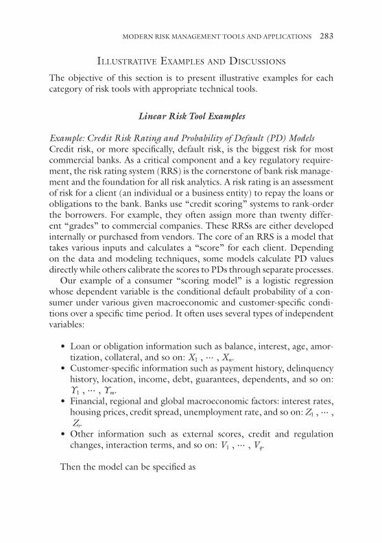
IllustratIve examples and dIscussIons

The objective of this section is to present illustrative examples for each category of risk tools with appropriate technical tools.

Linear Risk Tool Examples

Example: Credit Risk Rating and Probability of Default (PD) ModelsCredit risk, or more specifically, default risk, is the biggest risk for most commercial banks. As a critical component and a key regulatory require-ment, the risk rating system (RRS) is the cornerstone of bank risk manage-ment and the foundation for all risk analytics. A risk rating is an assessment of risk for a client (an individual or a business entity) to repay the loans or obligations to the bank. Banks use “credit scoring” systems to rank-order the borrowers. For example, they often assign more than twenty differ-ent “grades” to commercial companies. These RRSs are either developed internally or purchased from vendors. The core of an RRS is a model that takes various inputs and calculates a “score” for each client. Depending on the data and modeling techniques, some models calculate PD values directly while others calibrate the scores to PDs through separate processes.

Our example of a consumer “scoring model” is a logistic regression whose dependent variable is the conditional default probability of a con-sumer under various given macroeconomic and customer-specific condi-tions over a specific time period. It often uses several types of independent variables:

• Loan or obligation information such as balance, interest, age, amor-tization, collateral, and so on: X1 , ⋯ , Xn.

• Customer-specific information such as payment history, delinquency history, location, income, debt, guarantees, dependents, and so on: Y1 , ⋯ , Ym.

• Financial, regional and global macroeconomic factors: interest rates, housing prices, credit spread, unemployment rate, and so on: Z1 , ⋯ , Zs.

• Other information such as external scores, credit and regulation changes, interaction terms, and so on: V1 , ⋯ , Vq.

Then the model can be specified as

MODERN RISK MANAGEMENT TOOLS AND APPLICATIONS 283

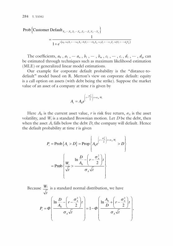
284

Prob Customer DefaultX X Y Y Z Z V Vn m s q

e

1 1 1 1

1

1

, , , , , , , , , , ,

{ }=

+ −− + + + + + + + + + + + +( )a a X a X b Y b Y c Z c Z d V d Vn n m m z s q q0 1 1 1 1 1 1 1 1

The coefficients, a0 , a1 , ⋯ an , b1 , ⋯ , bm , c1 , ⋯ , cs , d1 , ⋯ , dq, can be estimated through techniques such as maximum likelihood estimation (MLE) or generalized linear model estimations.

Our example for corporate default probability is the “distance-to- default” model based on R. Merton’s view on corporate default: equity is a call option on assets (with debt being the strike). Suppose the market value of an asset of a company at time t is given by

A A et

r t WAA t

=−

⋅ + ⋅

0

2

2σσ

Here A0 is the current asset value, r is risk free return, σA is the asset volatility, and Wt is a standard Brownian motion. Let D be the debt, then when the asset At falls below the debt D, the company will default. Hence the default probability at time t is given

P A D A e Dt t

r t WAA t

= >{ } = >

=

−

⋅ + ⋅

Prob Prop

Pr

0

2

2σσ

oobW

t

D

Ar t

tt

A

A

>− −

ln0

2

2

σ

σ

Because W

t

t is a standard normal distribution, we have

P

D

Ar t

t

A

Dr

t

A

A

A

=− −

= −+ −

Φ Φln ln

0

20

2

21

2

σ

σ

σ

t

tAσ,

Y. YANG

where Φ is the cumulative distribution function for the standard normal dis-

tribution and DTDt

t=

+ −

ln

A A

A

02

2Dr

σ

σ is called the distance-to-default.

However, this approach has a drawback: the asset value At and its volatility parameter σA are not directly observable. Instead, we can only observe the equity (stocks) Et and its volatility σE. Using Merton’s view and the celebrated Black-Scholes formula for option pricing, we obtain

E A

A

Dr t

tD e

A

Dt t

t A

A

rt

t

= ⋅+ +

− ⋅ ⋅+

−Φ Φln ln

σ

σ

2

2rr t

t

A

A

−

σ

σ

2

2.

To find the connection between σE and σA, we use Ito’s lemma to derive

σ σ

σ

σE t A t

t A

A

E A

A

Dr t

t⋅ = ⋅ ⋅

+ +

Φln

2

2

Using the historical stock prices Et and the two equations above, we can solve At and σA to find the default probability

P

A

Dr t

tDTDt

A

A

= −+ −

= − ( )12

1

02

Φ Φln

.

σ

σ

The probability Pt is often referred as point-in-time (PIT) PD or forward- looking PD as it incorporates the company’s stock price which often reflects the market expectation for the company’s future profits.


286

Example: Allowance for Loan and Lease LossesOne of the main applications of PD models is to calculate allowance for loan and lease losses (ALLL), or alternatively loan loss reserves (LLR) required by bank regulations and accounting standards. ALLL are reserves banks set aside to cover potential loan losses. Recently, two major accounting standards, the International Accounting Standards Board (IASB) and the Financial Accounting Standards Board (FASB), have proposed to adopt expected loss approaches for ALLL calculations: banks are required to estimate expected loan portfolio losses for one year from today and for the remaining loan life. Let us consider, for example, a portfolio whose loans have a maturity of twenty years. We assume that the loans in the portfolio could have various ages. It is understood that loans at different ages will have different default behaviors so a single PD is not sufficient to estimate the portfolio losses. Suppose the cumulative default probability up to age t is PD(t) and the lifetime PD is PD*. Then the function

F t

PD t

PDPD ( ) = ( )*

can be treated as a cumulative distribution function (CDF) with a prob-ability density function (PDF) ρ(t).

For each age t, suppose the portfolio has exposure Et for loans of age≤t.

Let E* be the total portfolio exposure and H tE

Et( ) =*

. The exposure has

a pdf wt which represents the portfolio weight of loans of age t. Then the one-year and the lifetime expected loss are calculated, respectively, as

OneYear ExpectedDefault Rate = ⋅ ⋅ +( ) − ( )( )∫

∞PD w F t F t dtt*

0

1

and

Lifetime Expected Default Rate = ⋅ ⋅ − ( )( )∫

∞PD w F t dtt* .

0

1

Y. YANG

Non-Linear Risk Tool Examples

Our previous example demonstrated that the default estimation for a portfolio could be complicated. Additional factors such as correlation and volatility can make the calculation even more challenging and less straight-forward. In statistics, correlation and volatility are second momentums that are non-linear in nature. Two important correlations are often used by risk tools. We started with an example of default correlation.

Example: Default Correlation of Bernoulli PortfolioDefault correlation is the correlation between default events of two loans. Let us consider a Bernoulli portfolio that has n loans. Each loan has one unit of exposure. Default is modeled as a binary event—either something defaults or does not. The default probability is p. Let us use a Bernoulli distribution i to indicate the default of ith loan. That is

i

th

th

i p

i=

( )1

0

if loandefaults withprobability

if loandoess default with probabilitynot p1−( )

.

Then the number of the defaults in the portfolio is L B==∑i

n

1i . Its vari-

ance is

Var Var

i

n

ii

n

j

n

i ji

n

j

n

L B B B( ) = ∑

= ∑ ∑ ( ) = ∑ ∑

= = = = =1 1 1 1 1Covar , ρii j i j, ⋅ ⋅σ σB B

Here ρi , j for i ≠ j is the default correlation between the ith and jth loan.

σ σ i jp p= = −( )1 is the standard deviation. ρi , i = 1 and

ρi j

i jand p

p p, == ={ }−

−( )

=

Prob ,

Joint Default Probabilityof

1 1

1

2

ii and j p

p p

th th loan −−( )

2

1

If we assume that the default correlations among any two loans are the same, then ρi , j = ρ and


288

Var np p p p np p

n n p p p p n

i jL( ) = −( ) + ∑ ⋅ −( ) = −( )

+ −( ) ⋅ −( ) = −( )≠

1 1 1

1 1 1

ρ

ρ ++ −( ) n n 1 ρ

So the standard deviation StDev n p pn n

( ) ( ) ( )

= = − + −Var 1

11

1ρ

. Since the portfolio has n loans, the probability of default for the portfolio

is PD =n

and its standard deviation is

StDev PDStDev

np p

n n

p p as n

( ) = ( )= −( ) + −

→ −( ) → ∞

1 1 1 1

1

ρ

ρ .

In other words, the default correlation can be directly estimated from the portfolio default volatility (or the standard deviation) StDev(PD):

ρ ≈

( ) −( )

StDev PD

p p

2

1

This is a quite simple but useful result for estimating default correla-tions for pools of retail loans using historical default data. This is a very popular method to derive the unobservable parameter ρ at the portfolio level. The next example will introduce another method that can simplify the loss calculation.

Example: Asset Correlation and Loss Distribution of Vasicek PortfolioThe default correlation derived from StDev ( ) is important. However, it won’t explicitly describe the calculation for the loss function . In fact, is a distribution that requires additional structure. Vasicek1 introduced a single-factor model where he assumed that each customer’s asset (after being normalized) was driven by a common systematic risk factor and an idiosyncratic risk factor. The loan will default if its asset falls below a threshold (the debt). More specifically, for ith customer, its asset is assumed to be

Y. YANG

A eiZ i= ⋅ + − ⋅θ θ ε1 .

Here Z is the standard normal distribution representing the systematic risk factor, εi is a normal distribution independent of Z and represents the idiosyncratic risk factor. θ is the asset correlation. The customer will default if the asset falls below D e p=

− ( )Φ 1

. Φ is the cumulative distribution function of the standard normal distribution.

Using the central limit theorem, Vasicek proved that as n → ∞, the loss

distribution n

approaches (weakly) to a heavy tail distribution whose

cumulative distribution function is given by

Prob * .≤{ } =− ⋅ ( ) − ( )

− −

xx p

ΦΦ Φ1 1 1θ

θ

In fact, conditional on the systematic risk factor Z, the loss distribution n

converges in probability to

L

n

Z p→

− ⋅ + ( )−

−

ΦΦθ

θ

1

1.

Example: Basel Capital Calculation Using Vasicek Distribution ModelOne important application of the Vasicek loss distribution model is the calculation of the capital requirement under Basel II internal rating based (IRB) Approach. Basel adopted the systematic versus idiosyncratic risk approach and proposed the following formula for calculating the minimal capital requirement for retail portfolios:

K LGDp

p MAdj=⋅ ( ) + ( )

−

−

− −

* * .ΦΦ Φθ α

θ

1 1

1

Here K is the capital requirement, LGD = loss given default, α = the confidence level (often 99.9%), and MAdj is the maturity adjustment. The


290

asset correlation θ is chosen based on the types of the loans. For example, θ = 0.15 for residential mortgages and θ = 0.04 for qualifying revolving retail exposures.

Basel capital is often called “supervisory” or “regulatory” capital. It is a prescribed risk measure that may not necessarily be based on bank’s indi-vidual risk profile. Its biggest advantages are that it is simple and additive (that is, the capital for a portfolio is the sum of the capitals for individual loans in the portfolio).

Example: Concepts of VaR, Economic Capital, Expected Shortfall, and Capital AllocationEconomic capital (or risk-based capital) is calculated based on banks’ internally derived risk methodologies and parameters. The idea is to cover extreme losses beyond expectation so the bank will stay solvent. It is always associated with a confidence level (often 99.9% or higher) to indicate the loss severity. For example, a 99.9% confidence level means to cover the worst yearly loss in 1000 years. Economic capital (EC) calculation requires the knowledge of full loss distribution. In fact, if is the portfolio loss distribution, then the required capital ECα ( ) for a given confidence level α can be defined as

Prob E ≤ ( ) + [ ]{ } =ECα α.

This definition directly relates economic capital to the popular value-at- risk (VaR) concept. In fact, it is easy to see

EC VaRα α ( ) = ( ) − [ ]E .

Furthermore, we have

I. If 1 2″ then, EC ECα α 1 2( ) ≤ ( ) . II. If λ > 0, then EC ECα αλ λ⋅( ) = ⋅ ( ) . III. For constant K, EC K ECα α +( ) = ( ) .

The main advantage of economic capital is its diversification benefit. In general, when two loss distributions 1 and 2 are combined, because the losses are not perfectly correlated, the EC for 1 2+ is often less than the sum of the two individual ECs. That is, people often expect to have

Y. YANG

EC EC ECα α α 1 2 1 2+( ) ≤ ( ) + ( ).

Unfortunately, this subadditivity is not always true. Criticisms of EC have led to the study of coherent measure of risk, which will be discussed later in this section. On the other hand, subadditivity might be an unre-alistic requirement and it is unreasonable to ask for diversification benefit when two companies are just combined arbitrarily. In real world, even the merger of two good companies could fail.

Economic capital is often calculated at the portfolio level. To be able to use EC for individual loans, it needs to be allocated to each loan. Because additivity does not hold for EC, the allocation is often tricky and has undesirable consequences. Three allocation methods are common. Let i be the loss distribution for the ith loan in the portfolio.

(1) Covariance Method: the EC for the ith loan is

E ECi iCStDevα α( ) ( )=

( )( )

Covar ,*

2

;

(2) Marginal Method: Let \ i be the portfolio without the ith loan and ∆α α α α

α α

α

t EC EC EC i

EC EC

EC

i

i

i

( ) = ( ) − ( ) ( ) =( ) − ( )

∑ ( )

\ ,

\

then

−− ( ) ( )

ECEC

iα α

\* .

(3) Euler Risk Contribution Method: EC i ECi iα α( ) ( ) [ ] [ ]= = + −E E E | .

Each of the above methods has some advantages as well as drawbacks. Both the covariance and marginal methods could produce zero or nega-tive capitals; the marginal method is often computational unfeasible, and the Euler risk contribution method needs Monte Carlo simulations and is often unstable.

To meet the subadditivity condition, expected shortfall (ES) has been proposed and suggested to replace EC. The ES can be defined as, assum-ing the condition ≥ ( )VaRα has non-zero probability,

ES VaRα α ( ) = ≥ ( ) − [ ]E E


292

That is, ES is the average of the losses that exceed the VaR ECα α ( ) = ( ) + [ ]E . In particular one obtains (assuming the con-dition ≥ ( )VaRα is not empty)

ES ECα α ( ) ≥ ( ).

It can be shown that the ES does satisfy the subadditivity (so it is a coherent risk measure):

ES ES ESα α α 1 2 1 2+( ) ≤ ( ) + ( )

However, the calculation of ES is extremely difficult and unstable as it requires the complete knowledge of the entire tail of (a seemingly impossible mission without significant assumptions regarding the tail). It is also nearly impossible to backtest ES. ES is created mainly to satisfy the subadditivity requirement, which seems in contradiction to certain merger and acquisition activities, as we pointed out earlier.

ES can also be allocated to individual loans following the covariance method or marginal method. Its Euler risk contribution method is: ES i VaRi iα α( ) = ≥ ( ) − [ ]E E .

Example: Capital and RAROCOnce EC is allocated to individual loans, banks often use risk-adjusted return on capital (RAROC) as a performance measurement tool to evalu-ate loan revenues and returns from a risk-oriented viewpoint. The idea is to view EC as a “common fund (or resource)” for risk and to adjust returns by expected losses for risk. For each loan, RAROC is often defined as

RAROC =

− −Revenues Expenses Expected Losses

Economic Capital

Most banks define hurdle rates (typically between 12% and 24%) and require RAROC to be higher than the hurdles.

RAROC can be used in portfolio optimization so banks can determine the optimal settings for the portfolio allocation or generate an efficient frontier that describes risk–return trade-off for the loans.

Y. YANG

Example: Copula and Loss Distribution for EC and ES calculationThe crux of EC calculation is the determination of portfolio loss distri-bution. As demonstrated by the Vasicek portfolio, the loss distribution is closely related to loan correlation. Banks often have many portfolios. Even if the loss distributions of individual portfolios have been derived, the aggregation of these loss distributions at bank level still presents a major challenge. For example, banks often have both retail loan portfolios and wholesale loan portfolios. If one has obtained the loss distribution R for the retail portfolio and W for the wholesale portfolio, then the aggregation of the retail and wholesale portfolios will have the loss distri-bution: R W R W∪ = + . To understand R W∪ , we need to understand the relationship between R andW . The first relationship is the linear correlation between them. However, correlation is a second momen-tum in nature (it only involves covariance and standard deviations). The calculation of EC requires the full loss distribution including information from higher momentums. This is why banks often use copula.

What is a copula? A copula is a way of describing the relationship between random variables. Why is copula is so popular? This is because copula can describe any relationship. To many people, copula is puzzling and difficult to understand. But it is really something quite natural.

They key to understanding copula is “rank order”. Before giving a pre-cise definition, we start with a practical question: if the retail portfolio suf-fers a big loss this year, what do we expect for the wholesale portfolio? To be more specific, if the retail portfolio suffers the worst loss in ten years, what about the loss for the wholesale portfolio? The answer could vary of course. For example, the wholesale portfolio could suffer a worst loss in five years, or it could suffer just the average loss. It could even suffer very little loss, so this year becomes the best year in ten years for the wholesale portfolio.

We now convert these descriptions into mathematical concepts and numbers. We rank the losses from the smallest to the largest (higher ranks correspond to higher losses). For example, the worst loss in ten years has a rank of 90%, the worst loss in five years has a rank of 80%, the average loss has a 50% rank, and the best year in ten years has 10% rank. Now our ques-tion becomes: if the retail portfolio has a loss at 90%, what is the loss rank for the wholesale portfolio? Our answer could be 80%, 50%, or even 10% or other ranks. Of course, 10% is very unlikely (or it has very low prob-ability). On the other hand, the probability for the wholesale portfolio to be at the 90% or 80% rank is higher. Please note that a rank or a probability


294

is always a number between zero and one. Now we are ready to give the definition of copula.

Definition A copula for distributions R and W is a function C(u, v) that satisfies the following conditions:

1. C(u, v) is between 0 and 1 for 0 ≤ u ≤ 1 , 0 ≤ v ≤ 1 (We can interpret that u and v are ranks for R and W ; C(u, v) is the probability for both R not to exceed rank u and W not to exceed rank v)

2. C(u, 0) = C(0, v) = 0 3. C(1, v) = v , C(u, 1) = u 4. For u1 ≤ u2 , v1 ≤ v2 , C(u1, v1) + C(u2, v2) − C(u1, v2) − C(u2, v1)

≥ 0

Conditions (2)–(4) are technical conditions to ensure C(u, v) a prob-ability function.

It is known that copula can be used to describe any relationship. This also implies that there are numerous types of copulae. The most common one is Gaussian copula which is just a different way of describing the lin-ear correlation. In the recent financial crisis, Gaussian copula was proven to severely underestimate the correlation in extreme situations hence is not appropriate for EC calculation. Other copulae include Clayton, Frank, and Gumbel. They are defined by a few parameters that can be calibrated through various methods.

To use copula for aggregating loss distributions, one needs to follow the following procedure.

1. Identify the right copula. For loss distributions, Gumbel is an ideal choice in many situations:

C u v eu v

,( ) =− − ( )( ) + − ( )( )

ln lnθ θ θ

1

2. Estimate the copula parameters. For Gumbel copula, it is θ. There are many estimation methods available. One could use either his-torical loss data or external loss proxy data (for example, data

Y. YANG

published by Federal Reserves). Assuming Fed data is used, we esti-mate that θ = 1.4 for retail and wholesale portfolios.

3. Simulate copula pairs: {(u1, v1), (u2, v2), (u3, v3), ⋯ , (un, vn)}. There are several efficient ways to simulate copulae and we probably need to simulate hundreds of thousands or even millions of pairs. Notice that this simulation is independent of R and W .

4. Use the simulated pairs to combine losses from R and W . This is the main step in loss aggregation. Precisely, for each simulated pair (uk, vk), take the rank uk loss Luk

from R and the rank vk loss Lvk

from W to calculate Z L Lk u vk k= +

5. Find EC or ES at the given confidence level α from the combined losses Zk. We first rank order the n combined loss values {Z1, Z2, ⋯ , Zn}. For EC, one would take the combined loss at the α rank. For ES, one would take all losses exceeding the α rank and average them. Finally one would subtract the average Z from EC or ES.

Transitional Risk Tool Examples

The credit quality of a client does not stay constant. It continuously evolves due to two main reasons: changes in internal business practices and changes in external business environment. Banks often categorize credit worthiness by status. For example, Basel banks assign 20+ risk rat-ings to the corporate clients and monitor various delinquency statuses of the retail customers. In each time period (monthly, quarterly, or annually), changes in client status are tracked and recorded using a matrix: a transi-tion matrix. Transition matrices provide a comprehensive and dynamic views on the risks in the portfolio.

Example: Risk Rating Transition MatrixAssume the bank has seven non-default ratings. The following is its aver-age annual transition matrix M (Table 1):

The matrix shows, for example, that in one year 80% of rating 4 cli-ents will stay at rating 4; 8% will be downgraded to rating 5; 2% will be upgraded to rating 3; and 7.5% will default.

There are essentially two types of transition matrices: by age or by cal-endar year.


296

1. Age-based transition matrix: we start with a group of new clients and keep track of their rating changes. The following is the transi-tion matrix at age 1 (Table 2).For clients initially rated at rating 4, one year later at age one, 81.3% will stay at rating 4, 7.1% will be downgraded and 3.4% will default.

2. Calendar-based transition matrix: for each year in the past, there was a transition matrix QYYYY (Table 3)

And (Table 4)When transition matrices are used, one often makes a very impor-

tant assumption: of Markovian property. That is, transition matrices are assumed to be time-homogeneous under matrix multiplication in the fol-lowing sense.

1. For age-based transition matrix Aage 1, the transition matrix at age N is A AageN age

N= 1 . For example, in first three years (age three), the probabilities are (Table 5):

2. For calendar-based transition matrices QYYYY, the matrix for the period 2012–2014 is Q2012 − 14 = Q2013 − 14 × Q2012 − 13 (Table 6)

Markovian property is very useful. However, it is also well-known that this assumption is often violated. While acceptable for many applications, its validity has to be carefully checked before one uses it. Here we give one application: what is the transition matrix in the first six months (i.e. at age ½ year)? The answer: the square root matrix of Aage 1 (Table 7).

Table 1 Average annual transition matrix

1 Year

1 2 3 4 5 6 7 D

1 90.0% 8.0% 1.5% 0.0% 0.0% 0.0% 0.0% 0.5%2 2.0% 85.0% 9.0% 2.0% 0.0% 0.0% 0.0% 2.0%3 0.0% 1.0% 83.0% 11.0% 1.5% 0.0% 0.4% 3.1%

M = 4 0.0% 1.0% 2.0% 80.0% 8.0% 1.0% 0.5% 7.5%5 0.0% 0.0% 0.0% 2.0% 75.0% 12.0% 2.0% 9.0%6 0.0% 0.0% 0.0% 0.0% 1.0% 70.0% 11.0% 18.0%7 0.0% 0.0% 0.0% 0.0% 0.0% 8.0% 60.0% 32.0%D 0.0% 0.0% 0.0% 0.0% 0.0% 0.0% 0.0% 100.0%

Y. YANG

This gives the credit deterioration pattern of a new portfolio in the first six months.

One can easily check: A Aage age age1 12

12

= × A

Special Risk Tool Examples

The recent financial crisis has led to significant changes in risk manage-ment regulations. Large banks are subject to intensified requirements such as CCAR or Basel II/III. These regulations are often designed to address specific concerns regarding banks’ safety and soundness, as well as their risk management practices. Common risk tools designed for business- as- usual (BAU) purposes may not necessarily meet the new (and evolving) supervisory goals and objectives. For example, CCAR banks have to rebuild almost all risk tools to perform the required stress testing by the

Table 2 Transition matrix at age one

Age 1

1 2 3 4 5 6 7 D

1 84.7% 9.3% 3.0% 1.4% 0.6% 0.5% 0.3% 0.2%2 0.8% 86.6% 9.3% 2.1% 0.4% 0.2% 0.2% 0.5%3 0.6% 2.8% 84.9% 8.2% 1.1% 0.4% 0.2% 1.9%

Aage1 = 4 0.0% 1.9% 5.5% 81.3% 7.1% 0.4% 0.4% 3.4%5 0.0% 0.0% 1.0% 5.4% 77.7% 7.0% 1.7% 7.1%6 0.0% 0.0% 0.1% 1.9% 5.3% 72.8% 6.2% 13.7%7 0.0% 0.0% 1.7% 3.4% 2.0% 15.5% 49.4% 28.0%D 0.0% 0.0% 0.0% 0.0% 0.0% 0.0% 0.0% 100.0%

Table 3 Transition matrix from 2012 to 2013

2012–2013 1 2 3 4 5 6 7 D

1 94.0% 5.0% 0.9% 0.0% 0.0% 0.0% 0.0% 0.1%2 0.0% 95.0% 4.0% 0.5% 0.0% 0.0% 0.0% 0.5%3 0.0% 2.0% 92.0% 4.0% 0.0% 0.0% 0.0% 2.0%

Q2012 − 13 = 4 0.0% 0.0% 6.0% 85.0% 3.3% 0.0% 0.0% 5.7%5 0.0% 0.0% 0.0% 2.0% 80.0% 5.0% 0.0% 13.0%6 0.0% 0.0% 0.0% 0.0% 5.0% 70.0% 4.0% 21.0%7 0.0% 0.0% 0.0% 0.0% 1.0% 10.0% 55.0% 34.0%D 0.0% 0.0% 0.0% 0.0% 0.0% 0.0% 0.0% 100.0%


298

Table 5 Transition matrix at age three

First 3 Yr

1 2 3 4 5 6 7 D

1 60.9% 20.7% 9.0% 4.2% 1.7% 1.2% 0.6% 1.5%2 1.8% 65.9% 20.9% 6.4% 1.6% 0.7% 0.4% 2.3%3 1.3% 6.8% 63.0% 17.5% 3.7% 1.1% 0.5% 6.1%

AageN = 4 0.1% 4.4% 12.2% 55.9% 13.9% 2.0% 0.9% 10.6%5 0.0% 0.4% 2.8% 11.0% 48.8% 12.7% 3.1% 21.1%6 0.0% 0.1% 0.8% 4.6% 9.6% 41.3% 7.4% 36.2%7 0.0% 0.3% 2.9% 5.7% 4.7% 18.2% 13.8% 54.4%D 0.0% 0.0% 0.0% 0.0% 0.0% 0.0% 0.0% 100.0%


2012–2014 1 2 3 4 5 6 7 D1 89.3% 9.3% 1.0% 0.0% 0.0% 0.0% 0.0% 0.3%2 0.0% 91.3% 7.2% 0.6% 0.0% 0.0% 0.0% 0.8%3 0.0% 2.9% 87.6% 6.4% 0.1% 0.0% 0.0% 3.0%

Q2012 − 14 = 4 0.0% 0.1% 8.2% 76.7% 4.5% 0.1% 0.0% 10.5%5 0.0% 0.0% 0.1% 3.4% 68.2% 6.4% 0.1% 21.8%6 0.0% 0.0% 0.0% 0.1% 7.2% 56.6% 5.4% 30.7%7 0.0% 0.0% 0.0% 0.0% 1.0% 12.1% 36.1% 50.8%D 0.0% 0.0% 0.0% 0.0% 0.0% 0.0% 0.0% 100.0%


2013–2014 1 2 3 4 5 6 7 D1 95.0% 4.8% 0.0% 0.0% 0.0% 0.0% 0.0% 0.2%2 0.0% 96.0% 3.7% 0.0% 0.0% 0.0% 0.0% 0.3%3 0.0% 1.0% 95.0% 3.0% 0.0% 0.0% 0.0% 0.9%

Q2013 − 14 = 4 0.0% 0.0% 3.0% 90.0% 2.0% 0.0% 0.0% 5.0%5 0.0% 0.0% 0.0% 2.0% 85.0% 3.0% 0.0% 10.0%6 0.0% 0.0% 0.0% 0.0% 4.0% 80.0% 4.0% 12.0%7 0.0% 0.0% 0.0% 0.0% 0.0% 8.0% 65.0% 27.0%D 0.0% 0.0% 0.0% 0.0% 0.0% 0.0% 0.0% 100.0%

Y. YANG

Tab

le 7

Sq

uare

roo

t tr

ansi

tion

mat

rix

at a

ge 1

/2

Age

1/2

12

34

56

7D

192

.00%

5.00

%1.

50%

0.70

%0.

30%

0.25

%0.

20%

0.05

%2

0.40

%93

.00%

5.00

%1.

00%

0.20

%0.

10%

0.10

%0.

20%

30.

30%

1.50

%92

.00%

4.50

%0.

50%

0.20

%0.

10%

0.90

%Aage1 2

=4

0.00

%1.

00%

3.00

%90

.00%

4.00

%0.

11%

0.20

%1.

69%

50.

00%

0.00

%0.

50%

3.00

%88

.00%

4.00

%1.

00%

3.50

%6

0.00

%0.

00%

0.00

%1.

00%

3.00

%85

.00%

4.00

%7.

00%

70.

00%

0.00

%1.

00%

2.00

%1.

00%

10.0

0%70

.00%

16.0

0%D

0.00

%0.

00%

0.00

%0.

00%

0.00

%0.

00%

0.00

%10

0.00

%


300

Fed. The key is to establish linkages between the nineteen macroeconomic factors forecasted by the Fed and banks’ risk models. In technical terms, all established risk parameters have to be reformulated conditional on macro-economic factors. This is quite interesting because banks often tried not to link their BAU models to macroeconomic variables in the past as this could lead to unnecessary volatility in loss estimations.

Example: Balance ForecastingOne of the CCAR models that is very different from standard risk man-agement tools is the balance/income forecasting model. In general, the balance or volume of a portfolio is a consequence of business activities and banks often incorporate its forecast into budget process, not through risk models. However, due to the unique requirement of CCAR for risk- weighted asset (RWA) and capital planning, banks have to build mod-els to link the balances to macroeconomic variables. Depending on the data quality and availability, balance models are commonly developed at aggregated levels, and regression-based time series approach is the main methodology.

For example, the bank has observed the month-end balances of its direct installment real estate portfolio over the past 10 years. Given this time series of 120 data points, it models the percentage change in port-folio balance as a linear regression of the nineteen Fed macroeconomic variables (including HPI, GDP, unemployment rate, stock market, inter-est rate, and so forth). The model is finalized as ∆ ∆ ∆ ∆Balance a a HPI a InterestRate a Unemploymentn n= + + + +0 1 2 3* * * .

Example: PD ForecastingThe PD models we discussed earlier also need to be redesigned to incor-porate macroeconomic factors. For example, PIT PD which is driven by distance-to-default, can be linked to macroeconomic factors in two ways. The first is to forecast company’s financials in the future. As both the equity volatility and stock index are forecasted by the Fed, one can apply the asset–equity relationship equations introduced at the beginning of this chapter to estimate the PIT PD under various scenarios. However, the forecast for a company’s financials and capital structure is not easy and often inaccurate. This approach contains a lot of uncertainties.

Y. YANG

The second approach is more practical. We take the historical PIT PD series of the company:

PD PD PDn1 2, ,,{ }

and use the relationship PD = 1 − F(DTD) to back out the DTD time series by DTD = Φ−1(1 − PD)

DTD DTD DTDn1 2, , ,{ }.

In fact, for any given historical PD series {p1, p2, ⋯ , pn}, one can con-vert it to a DTD series by applying the Probit transformation Φ−1(1 − p)

DTD p DTD p DTD pn n1

11 2

12

11 1 1= −( ) = −( ) = −( ){ }− − −Φ Φ Φ, , , .

Now we can use regression or other time series techniques to link {DTD1, DTD2, ⋯ , DTDn} to macroeconomic factors, and to forecast DTD under various scenarios. We can then use PD = 1 − Φ(DTD) to convert the forecast DTD back to PD.

Example: Alternative to Conditional Transition MatrixCCAR is often performed in using the conditional transition matrix approach. However, to directly link transition matrices to macroeconomic factors is very challenging and the common method is to use logistic regressions to model each entry of the matrix. But this approach suffers several significant drawbacks. There are too many regressions to be built. These regressions cannot keep the integrity of a transition matrix and some matrix regularization process is needed at the end of the forecast. Many matrix entries also do not have sufficient observations to run regressions. Each regression may have different drivers with varying performance.

Here we introduce an alternative. It is easy and intuitive with very few regressions to perform.

Suppose we use a risk rating system with K rating grades (so our transi-tion matrices are K by K). Let us consider our historical transition matrices

, , , , , , , ,Q Q Q Q Q Q QQ Q Q Q Q Q Q2000 1 2000 2 2000 3 2013 1 2013 2 2013 3 2013 44 ,{ }.


302

Suppose our current portfolio has, for rating j, exposure Ej

(j = 1, 2, ⋯ , K). Consider the exposure vectors: W0

1

2=

EE

EK

, and calculate

W Q Q WYYYY YYYY YYYY=

=* *

EE

EK

1

20

(if we are forecasting for longer period,

W0 needs to multiplied by more transition matrices). This generates a series of vectors

,W ,W ,W , ,W ,W ,W ,WQ Q Q Q Q Q Q2000 1 2000 2 2000 3 2013 1 2013 2 2013 3 2013 44 ,{ }

Notice that the last element in each W vector is the defaults that rep-resent the estimated historical defaults for the current portfolio for each historical period. Then we apply common regression or time series tech-niques on these “estimated historical defaults” with respect to macro-economic factors. This way, we can forecast future losses of the current portfolio without using any conditional transition matrices.

conclusIons

Several modern risk management tools have been developed to address many risk management problems in the wake of financial crisis of 2007–2008. In this chapter I have introduced these modern tools and explained them in appropriate technical detail by using illustrative exam-ples for how these tools are used in current market practice.

note

1. Oldrich At Vasicek, Loan portfolio value, December, 2002, www.risk.net.

Y. YANG

http://www.risk.net

Risk Management and Technology


GRC Technology Introduction

Jeff Recor and Hong Xu

J. Recor () Grant Thornton , 27777 Franklin Road, Suite 800 , Southfi eld , MI 48034 , USA

H. Xu American International Group , 614 Ashgrove Ln , Charlotte , NC 28270 , USA

The view expressed in this paper represents the personal opinion of authors and not those of their current and previous employers.

INDUSTRY DESCRIPTIONS OF GRC Over the past decade, organizations have been using different technologies and approaches to automate their risk and compliance management functions. Technologies such as spreadsheets and word processor programs have been commonly used to provide organizations with the ability to list and track risks, controls and assessment processes, issues, and remediation. As organizations looked to improve upon the use of spreadsheets, different combinations of workfl ow, database and reporting technology solutions have been created to address risk and regulatory challenges. It is generally accepted that around 2002, a new marketplace acronym was created to encapsulate these technology solu-tions into a category called “governance, risk, and compliance” (GRC).

Vendors were quick to latch on to the new market acronym as a way to position their solutions to include partial or full integration between workfl ow, database, and reporting capabilities packaged into an inte-grated platform.

Several recent studies have shown how much the GRC marketplace has grown. A study conducted by Markets and Markets (GRC market trends 2013–2018) shows the eGRC solutions (software) market is expected to grow from $3.21 billion in 2013 to $6.27 billion in 2018 at a compound annual growth rate (CAGR) of 14.3% during the forecast period. OCEG (formerly called the Open Compliance and Ethics Group) recently per-formed a technology strategy survey (results published January 2016) that shows 55% of those polled are going to be increasing their spending on GRC (and another 18% are keeping spending the same).

With a growing reliance upon GRC technology platforms, the next two chapters will examine how organizations are gaining value from leverag-ing an integrated platform. Realizing that there are many different tech-nologies that can fall under the acronym for GRC, this chapter will focus on those solutions that are marketed and sold as integrated platforms for automating GRC functions. The authors will rely upon observations from actual GRC projects performed for clients across multiple industries in order to show common approaches used in order to gain benefi ts through the use of a GRC technology platform.

The topic of GRC technology can often be confusing and lack spe-cifi c solution defi nitions. In 2002, a market analyst (or a Big 4 consultant depending on who you ask) is generally acknowledged as making the term GRC more mainstream by grouping together risk and compliance tech-nology capabilities for comparison purposes. An early defi nition of GRC usually involved a blending of people, processes and software to assist with addressing regulatory (compliance) requirements.

There are many different technical capabilities that can qualify as sup-porting governance, risk, or compliance solutions. The challenge has been to leverage a technical capability that can enable integration across mul-tiple people, processes, and requirements. The marketplace has evolved from providing solutions to address specifi c regulatory needs to a more broad-based support platform. Even though the GRC technology platform vendors (and clients) have had roughly a decade to mature their respec-tive solutions, there is still some confusion as to what constitutes a GRC solution. Vendors, standards bodies, think tanks, and marketplace analysts

306 J. RECOR AND H. XU

have been working to provide a more formal defi nition for GRC. Here is a description that includes some of the more prominent defi nitions:

OCEG (Formerly the Open Compliance and Ethics Group)

OCEG is a global nonprofi t organization that develops and provides standards, guidelines, tools, and other resources to address governance, risk, and compliance management (GRC) for organizations of all sizes. All OCEG guidance is publicly vetted and fi nalized following a public com-ment period and testing of the application of the guidance within one or more organizations. The guidance is further augmented by development of online resource collections and toolkits that enable users to swiftly and effi ciently customize and apply the guidance within their organizations. The guidance and all related resources are contained in a searchable data-base that OCEG member organizations can freely access. Membership in OCEG is free and can be accessed at www.oceg.org .

OCEG has developed several resources: The GRC Capability Model: (known as the Red Book), is a process

model for the design, operation and evaluation of GRC programs. It is supported by several guides, such as:

– The GRC Technology Solutions Guide : explains how GRC solutions are comprised of 28 different solution categories. http://www.oceg.org/resources/grc-technology-solutions/

– The GRC Assessment Tools Guide : (known as the “Burgundy Book”), enables organizations to examine their GRC capabilities across the enterprise, a division or a single project through the use of established and agreed upon procedures. http://www.oceg.org/resources/grc-assessment-tools-burgundy-book/

At the core of OCEG’s work is a very good defi nition for GRC:

A capability that enables an organization to reliably achieve objectives while addressing uncertainty and acting with integrity includes the governance, assurance, and management of performance, risk, and compliance. For OCEG, GRC is about taking an integrated approach for achieving prin-cipled performance.

OCEG’s GRC Technology Solutions Guide outlines 28 aspects of solutions that make up the GRC ecosystem as follows:

GRC TECHNOLOGY INTRODUCTION 307

http://www.oceg.org

http://www.oceg.org/resources/grc-technology-solutions/

http://www.oceg.org/resources/grc-technology-solutions/

http://www.oceg.org/resources/grc-assessment-tools-burgundy-book/

http://www.oceg.org/resources/grc-assessment-tools-burgundy-book/

• Audit & Assurance Management; • Board & Entity Management; • Brand & Reputation Management; • Business Continuity Management; • Compliance Management; • Contract Management; • Control Activity, Monitoring, and Assurance; • Corporate Social Responsibility; • eDiscovery Management; • Environmental Monitoring and Reporting; • Environmental Health & Safety; • Finance/Treasury Risk Management; • Fraud & Corruption Detection, Prevention & Management; • Global Trade Compliance; • Ethics Hotline/Helpline; • IT Risk & Security; • Insurance & Claims Management; • Intellectual Property Management; • Issues & Investigations Management; • Matter Management; • Physical Security & Loss Management; • Policy Management; • Privacy Management; • Quality Management and Monitoring; • Reporting & Disclosure; • Risk Management; • Strategy, Performance, and Business Intelligence; • Third Party/Vendor Risk and Compliance.

The Institute of Internal Auditors

The Institute of Internal Auditors (IIA) is the internal audit profession’s global voice, recognized authority, acknowledged leader, chief advocate, and principal educator. Generally, members work in internal auditing, risk management, governance, internal control, information technology audit, education, and security.

Globally, The IIA has more than 180,000 members. The IIA in North America comprises 160 chapters serving more than 72,500 members in the USA, Canada, the Caribbean (Aruba, Bahamas, Barbados, Cayman


Islands, Curacao, Jamaica, Puerto Rico, and Turks and Caicos), Bermuda, Guyana, and Trinidad and Tobago.

The IIA slightly changes the acronym defi nition for GRC to be, “governance, risk and control”. In August of 2010 the IIA adopted sup-port for the OCEG defi nition for GRC and added that GRC is about how you direct and manage an organization to optimize performance, while considering risks and staying in compliance. IIA stated clearly:

– GRC is NOT about Technology; – GRC is NOT a fad or a catchy phrase for software vendors and

professional service providers to generate revenue.

The Institute of Risk Management

The Institute of Risk Management (IRM) lists on its website this defi ni-tion for GRC:

GRC is a term used to describe an integrated approach to activities related to governance, risk management and compliance. Increased corporate failures and enhanced regulatory requirements have heightened corporate aware-ness about the value and importance of making sure these key activities are effectively designed, integrated and managed.

Prominent information technology analyst fi rms have performed an impor-tant service for clients by helping to produce opinions on which GRC software vendor may be the best fi t based on specifi c use cases. While an argument can be made that those opinions may not be accurate or entirely objective, in many cases these opinions are the only sources of information on leading GRC vendors that organizations use to select potential solu-tions (or that are available other than from the vendors themselves). Due to the infl uence that some of these analysts have with clients, it is worth noting how they have defi ned GRC for client consumption. Since there are many different market analysts that cover the GRC marketplace we are going to only pick a representative sample using Forrester and Gartner to show an example of the types of defi nitions used to defi ne GRC.


Forrester Research

Forrester Research describes itself as, “one of the most infl uential research and advisory fi rms in the world. We work with business and technol-ogy leaders to develop customer-obsessed strategies that drive growth. Forrester’s unique insights are grounded in annual surveys of more than 500,000 consumers and business leaders worldwide, rigorous and objec-tive methodologies, and the shared wisdom of our most innovative clients. Through proprietary research, data, custom consulting, exclusive execu-tive peer groups, and events, the Forrester experience is about a singular and powerful purpose: to challenge the thinking of our clients to help them lead change in their organizations” www.forrester.com .

Analysts at Forrester were some of the earliest users of the abbreviation GRC. Forrester has been well-known for producing research and more specifi cally a product called the GRC Wave that clients can use to help make decisions about GRC software vendors. Forrester’s work in the GRC space is summarized on their website as follows: “Every organizational business function and process is governed in some way to meet objec-tives. Each of these objectives has risks, as well as controls that increase the likelihood of success (or minimize the impact of failure). These are the fundamental concepts of GRC. To maximize business performance, GRC programs are designed to help companies avoid major disasters and minimize the impact when avoidance is unlikely” https://www.forrester.com/Governance-Risk-%26-Compliance-%28GRC%29 .

According to Forrester, the Forrester Wave is a collection of informa-tion from vendor briefi ngs, online demos, customer reference surveys and interviews, use of Forrester’s own demo environment of each vendor’s product, and, as per Forrester policy, multiple rounds of fact checking and review. The current iteration of the Forrester Wave was previously split into two distinct reports- one for enterprise GRC (eGRC) and the other for IT GRC. Trying to defi ne the distinction between enterprise and IT GRC has added to some of the marketplace confusion around GRC platforms.

In addition to products like the GRC Wave, Forrester has started to build what it calls a GRC Playbook. The playbook gives Forrester a new way to package up important research and guides within the following categories:

– Discover – Plan


http://www.forrester.com

https://www.forrester.com/Governance-Risk-&-Compliance-(GRC)

https://www.forrester.com/Governance-Risk-&-Compliance-(GRC)

– Act – Optimize

The Forrester GRC Playbook was completed at the end of 2015.

Gartner

Here is the description of Gartner’s focus in the marketplace from its website:

Gartner, Inc. (NYSE: IT) is the world’s leading information technology research and advisory company. We deliver the technology-related insight necessary for our clients to make the right decisions, every day. From CIOs and senior IT leaders in corporations and government agencies, to business leaders in high-tech and telecom enterprises and professional services fi rms, to technology investors, we are the valuable partner to clients in approxi-mately 10,000 distinct enterprises worldwide.

Through the resources of Gartner Research, Gartner Executive Programs, Gartner Consulting and Gartner Events, we work with every cli-ent to research, analyze and interpret the business of IT within the con-text of their individual role. Founded in 1979, Gartner is headquartered in Stamford, Connecticut, USA, and has 7,600 associates, including more than 1,600 research analysts and consultants, and clients in 90 countries. www.gartner.com

Prior to 2014, Gartner produced research for clients on the various GRC vendors in the form of MarketScope and Magic Quadrant reports. Similar in structure to Forrester’s Wave reports, the Gartner Magic Quadrant was a collection of vendor data measured against criteria that produced a rank-ing similar in format to the Forrester Wave.

In 2014 Gartner announced it was doing away with the Marketscope and Magic Quadrant reports and retooling its research on the GRC mar-ket to be more focused on specifi c use cases. According to a report from Gartner released on May 13, 2015 entitled, “Defi nition: Governance, Risk and Compliance”, Gartner provides this defi nition for GRC:

Governance, risk and compliance (GRC) is a set of practices and processes, supported by a risk aware culture and enabling technologies, that improves decision making and performance through an integrated view of how well an organization manages its unique set of risks.


http://www.gartner.com

http://www.gartner.com

In the same report, Gartner goes on to explain that, “there are a growing number of GRC software applications that automate various workfl ows in support of GRC goals. Through common functions such as an asset repository, regulatory mapping, survey capabilities, workfl ow functions and data import, GRC automation addresses multiple use cases defi ned by Gartner. The seven defi ned Gartner GRC use cases are as follows:

– IT Risk Management – IT Vendor Risk Management – Operational Risk Management – Audit Management – Business Continuity Management Planning – Corporate Compliance and Oversight – Enterprise legal Management.”

We are not trying to present an opinion on the merits of how the GRC marketplace is viewed or defi ned. The information presented here shows how many different fi rms view the marketplace for GRC technology plat-forms. As you will read in the following sections, integration of an organi-zation’s governance, risk, and compliance (control) functions is absolutely key when it comes to gaining value from automation. Any defi nition that does not support leveraging an integrated technology approach is prob-ably not going to gain much momentum in the marketplace.

GRC SCOPE OF COVERAGE An additional consideration for examining how GRC is defi ned is the scope of coverage for capabilities offered by GRC platform vendors. In addition to marketplace coverage provided by the analyst fi rms, GRC vendors have been positioning themselves in specifi c ways which also can cause confusion when it becomes time to evaluate technical capabilities. Basically, GRC vendor capabilities can be divided into three general cat-egories (Fig. 1 ).

This simplistic view of GRC vendor capabilities is starting to change as more organizations mature with their GRC processes and as vendors invest to build more integrated capabilities within their platforms.

As enterprise resource planning (ERP) vendors add more capabilities that have been traditionally found within GRC platforms the differences between them start to get blurred. Many organizations have both ERP and GRC platforms. The reasons for this are varied, but many of the ERP


vendors were slow to adopt capabilities that IT needed in order to be nim-bler, such as performing self-assessments, control harmonization, policy management, compliance testing and reporting, vendor risk management, vulnerability management, incident management, and several other functions.

There has been some confusion with GRC vendors in establishing their capabilities as being able to support eGRC (enterprise GRC) or IT GRC. Up until recently the distinction was focused around whether a platform would support enterprise risk management (ERM) capabilities, business performance management (BPM) and other enterprise functions, or was just focused on capabilities marketed to support IT functions (IT GRC). Market analysts, until recently, even supported two distinct views of vendors along these lines. We are now fi nding that as organizations have matured their GRC programs and level of integration, this distinction for technology support is diminishing.

The specialty GRC market still exists, but is increasingly shrinking due to the development of integrated capabilities in the other two categories. Solutions that once were marketed to solve a specifi c challenge such as contract management, case management, and others are now being inte-grated into GRC technology platform functionality.

ERP GRC Specialized

• Financial controls monitoring

• Risk monitoring

• Performance and operational controls

• Access & segregation of duties controls

• Enterprise risk management• IT GRC• Compliance management• Vendor risk management• Policy management• Audit management• Threat and vulnerability

management

• Environmental health and safety• Sustainability performance

management• Medical compliance• Food and Safety compliance• Legal case management• Other stand alone solutions

Core functions:

• Enterprise Resourcing Planning integrates various financial control functions into one complete system across the entire organization. The central feature of all ERP systems is a shared database that supports multiple functions used by different business units. Only recently have functions related to IT GRC capabilities been added to ERP systems.

Core functions:

• The early focus of GRC platforms was to address compliance reporting and risk and control self assessments. Other common solutions include vendor risk management and inciddent management. As GRC process maturity improves, more of these point solutions become integrated and can be leveraged across the enterprise.

Core functions:

• Most of the specialized GRC capabilities address a unique problem that has not typically gone through process integration. As organizations mature with their GRC process capabilities, the market demand for stand alone / specialized technology solutions diminishes.

Fig. 1 GRC Vendor Domain Capabilities


The term GRC today can invoke strong feelings of support or apathy. There are some practitioners who feel that the term GRC is too gen-eral and does not represent anything new that organizations should be doing. The feeling is that there is no such thing as a GRC department, so undertaking projects that involve improving processes and technology specifi cally as GRC does not accurately represent the operations of most businesses. Organizations have been leveraging automation to improve the governance, risk management, and compliance management functions before there was a new integrated platform capability in the marketplace to leverage.

As shown above, it is very common for the GRC concept to be associ-ated with technology solutions rather than as a business-oriented solutions approach. Despite the different interpretations of GRC being discussed and addressed, there is one common theme that stands out in these dis-cussions: clients view the automation and enterprise integration of gov-ernance, risk, and compliance programs as critical areas for achieving effi ciency gains, improved transparency, and better control.

GRC PROGRAM OVERVIEW Governance, risk, and compliance solutions are often looked at through the lens of their individual defi nitions. While true that the “G”, “R”, and “C” all have established defi nitions by various standards bodies and prac-titioners, organizations still struggle at performing some tasks within and across each of these programs. GRC technology platforms can provide value independently within each of these disciplines. However, as we will describe in more detail later in this chapter, it is the ability to leverage integrated capabilities that can assist an organization with making truly impressive performance improvements. As a refresher, there follow the formal defi nitions for each of the respective programs.

Governance

Corporate governance is the system of rules, practices, and processes by which organizations are directed and controlled. Corporate governance of IT is the system by which the current and future use of IT is directed and


controlled. Corporate governance of IT involves evaluating and direct-ing the use of IT to support the organization and monitoring this use to achieve plans. It includes the strategy and policies for using IT within an organization.

Defi nition from ISO 38500, Corporate Governance of Information Technology.

ISO 38500 also lists six principles that should be followed to provide good corporate governance of IT:

– Responsibility; – Strategy; – Acquisition; – Performance; – Conformance; – Human Behavior.

Directors of organizations are encouraged to govern IT by using a model to evaluate, direct, and monitor. It is important to note that gover-nance establishes the method for the organization’s processes to be man-aged (the “what”), but is not operational management (the “how”). ISO 38500 is a good resource for the responsibility of the board of directors in establishing the high-level requirements of governance of IT.

To apply these concepts as a GRC program that delivers value and pro-tects against risk, typical governance functions can include the following:

– Executive oversight; – Policy management; – Strategy; – Financial management; – Portfolio management; – Risk management.

One of the important elements of an overall risk governance approach to note is the establishment of the three lines of defense model. Since the fi nancial crash of 2008, the three lines of defense model has been receiv-ing more attention as a means to promote clear accountability for risk tak-ing, oversight, and assurance within organizations. The basic premise to the model is as follows:

First line of defense: functions that own risk;


second line of defense: functions that oversee risks; third line of defense: independent review function (internal audit).

There are many practitioners that feel this model is not a good representa-tion of how to effectively manage risk. The model is included here due to its prominence as part of the Basel Commission on Banking Supervision Operational risk requirements for banks. For fi nancial institutions, this model is a core part of a GRC program.

The use of GRC technology platforms to support functions related to governance can have a big impact on helping to track and improve the performance of the organization. There are many benefi ts to leveraging automation to support governance functions:

– Provides more timely, accurate, and reliable information; – Enables more informed decision-making for allocating resources; – Saves costs by improving effi ciency and reducing manpower hours

needed for administrative tasks related to reporting, policy man-agement lifecycle, and executive oversight tasks;

– Assists in improving performance management by providing inte-grated processes, accountability, and reporting;

– Supports a culture of process improvement.

Strictly from a technology support capability standpoint, there are many solutions that would fall under the governance category. Leveraging automation to support governance functions is an important and often diminished component of a fully integrated GRC program. Examples of governance functions that can take advantage of automation through a GRC technology platform include:

– Whistleblower hotline tracking and monitoring; – Board of directors reporting; – Corporate strategy approval tracking; – Executive compensation linked to corporate performance; – Policy management; – Performance management; – Strategic objective monitoring; – Portfolio management; – “What-if” analysis for budgeting/resource allocation; – Executive dashboard and reporting.


Developing solutions to support governance functions has been rela-tively slow compared with other risk and compliance functions. However, applying automation to support the monitoring of corporate performance and meeting objectives should not be overlooked in importance as part of a solution roadmap. In fact, it is common for us to see organizations continuing to improve their governance capabilities as they build and integrate other risk and compliance related solutions and information. As an example, we are seeing organizations link objectives with their corresponding risks as they mature in the use of a risk domain structure enabled in a risk register. Whether the risk register is populated in a bot-tom-up fashion (through capturing results of risk assessments and other activities) or a top-down approach (through facilitated sessions to capture core enterprise risks) has the added benefi t of gaining better visibility into risks, objectives, and performance over time.

Also, organizations are gaining direct benefi ts for their governance functions through many of the integration efforts that break down silo activity, fragmented approaches, disparate operations, duplicated efforts, dysfunctional communication mechanisms, and other improved opera-tional effi ciencies.

Risk Management

There are a number of risk management standards that organizations can use to help defi ne a formal program. A widely accepted defi nition from ISO 31000 states:

Risk Management aids decision making by taking account of uncertainty and its effect on achieving objectives and assessing the need for any actions.

The standard goes on to describe the following functions as part of the risk management process:

– Establishing the context; – Identifying, analyzing, evaluating, and treating risk; – Monitoring and reviewing risk; – Recording and reporting the results; – Communication and consultation throughout the process.


ISO 31000 also defi nes the following principles of risk management:

– create value—resources expended to mitigate risk should be less than the consequence of inaction;

– be an integral part of organizational processes; – be part of decision-making process; – explicitly address uncertainty and assumptions; – be a systematic and structured process; – be based on the best available information; – be tailorable; – take human factors into account; – be transparent and inclusive; – be dynamic, iterative and responsive to change; – be capable of continual improvement and enhancement; – be continually or periodically reassessed.

However, organizations continue to struggle with the achievement of many of their risk management goals. Critical risk exposures continue to exist despite large investments to improve risk management capabilities. Even though risk management technology capabilities are typically mar-keted by GRC vendors as improving the ability to reduce or eliminate risk (or improve the effi ciencies of managing risk), the ability to provide better visibility into risks means organizations can take advantage of the positive aspects that risk mitigation can enable in the decision-making process. This important aspect of risk management is often overlooked as organi-zations continue to automate some of the more mundane tasks related to fi nding, managing, and monitoring risks.

Risk management functions can be some of the most complex capabili-ties to automate consistently across the enterprise. Many functions related to risk management have been slow to leverage technology support, or are using automation in a limited capacity such as tracking enterprise risks using a spreadsheet. There are many benefi ts to leveraging automation to support risk management functions:

– Better visibility into risk; – Enables better decision-making for leveraging risk for positive

gain; – Can save costs by improving effi ciency and reducing manpower

hours needed for performing risk assessment, risk treatment, and risk monitoring tasks;


– Provides the capability of correlating and analyzing many data sets to help identify and treat emerging risks more effi ciently than manual processes;

– Provides ability to establish and manage a risk appetite and over-all risk posture that can support decision-making and investment “what if” scenario planning;

– Supports a culture of risk awareness.

Of course, GRC technology platforms work in conjunction with improvements to people and processes. Even though there are short-term benefi ts to be gained by making tasks related to the risk management func-tion more effi cient and interconnected, the real value comes from improv-ing risk management capabilities to support effective decision-making and breaking down silos within the risk management domain.

Compliance Management

Failing to understand regulatory requirements or having the right con-trols and culture in place can cost organizations in heavy fi nes and reme-diation efforts. Automating compliance processes was one of the early use cases for the acquisition of GRC technology platforms. Compliance man-agement programs involve more than just managing a checklist of which controls are required by which regulations. However, until recently there has not been much in the form of guidance from standards bodies about the functions a good compliance management program should contain. It has been common to observe organizations that were managing risks through the compliance checklist approach. In other words, if an organi-zation could prove through testing that all controls required by regulatory requirements were in place and operating effectively, those risks would be, generally speaking, in check.

Recent guidance has been released to help organizations understand leading practices associated with the compliance management function. For example, the FFIEC (Federal Financial Institutions Examination Council) Compliance Examination Manual listed the activities a compli-ance management system should perform as part of the overall risk man-agement strategy of an organization as follows:

– Learn about its compliance responsibilities; – Ensure that employees understand the responsibilities;


– Ensure that requirements are incorporated into business processes; – Review operations to ensure responsibilities are carried out and

requirements are met; – Take corrective action and update materials as necessary.

The International Standards Organization (ISO) has recently come out with a new international standard that provides guidance for compliance man-agement systems (CMS). ISO 19600:2014 provides guidance for establishing, developing, implementing, evaluating, maintaining, and improving an effective and responsive compliance management system within an organiza-tion. Similar to the FFIEC guidance, the core tasks that fall within this model include:

– Identifying compliance obligations; – Evaluate compliance risks; – Defi ne and implement measures; – Monitor controls; – Review the compliance management program continuously; – Manage noncompliance.

The introduction of ISO 19600 outlines the minimum guidelines and standards that are expected to be in place for a compliance program to be effective.

Compliance with an overwhelming amount of new laws, rules, and reg-ulations continues to be one of the key driving (marketing) forces behind the growth of GRC technology solutions. Some of the biggest gains in effi ciency and cost savings can be achieved by leveraging GRC technology platforms to address regulatory requirements and reporting. However, in order to obtain bigger gains in cost savings and effi ciencies these technol-ogy platforms need to be paired with integrated processes and content libraries. There are many benefi ts to leveraging automation to support the above mentioned compliance functions:

– A reduction in the amount of controls required to manage risks; – Ability to risk rationalize controls; – Cost savings by improving effi ciency and reducing manpower

hours needed for tasks related to control testing and reporting; – Improvement in quality of information related to risks and

controls; – Ability to focus resources to areas of the business that need the

help;


– Provide better reporting; – Identify testing biases; – Identify patterns of exceptions that may not fi t business objectives.

Integration

As GRC technology has matured it has become easier to make a busi-ness case that clearly articulates the process improvements, effi ciencies, and cost savings that can be achieved leveraging GRC technology for spe-cifi c use cases. However, just because technology can be utilized does not mean that by itself benefi ts will be realized. Many of the effi ciency gains and cost savings are dependent on solid processes, clear direction, orga-nizational cooperation, and support of the right technical capabilities. We have seen many GRC projects fail, or simply not return the effi ciency/cost savings gains that were planned due to a lack of awareness about the role that integration plays.

The marketplace is starting to use the term “integrated” related to GRC in several different ways. There are some organizations that tout an “integrated GRC capability”. Others tout the integration that occurs between GRC programs, and still others mention integration benefi ts in relation to interconnecting disparate data and systems. What tends to get lost in the messaging is what is actually meant by “integration” and how additional benefi ts can be derived if the effort to integrate the various functions related to GRC programs can be realized.

In our experience, the term “integrated GRC” is redundant. Integration is not something you apply to your GRC programs per se, but rather drive through people, process, and technology improvements and innova-tion. As increased levels of integration are implemented, greater benefi t can be achieved through all of the GRC functions. Ultimately, leveraging integration through the improvement of GRC processes will enable the connectivity between risks, strategy, and performance that can guide an organization to achieve its overall objectives.

The think tank OCEG has pulled together some very good guidance related to the topic of integration and its impact on driving principled per-formance, which is defi ned as a point of view and approach to business that helps organizations reliably achieve objectives while addressing uncertainty and acting with integrity. We believe OCEG is correct in guiding organiza-tions to, “... achieve principled performance - the capabilities that integrate


the governance, management and assurance of performance, risk and compli-ance activities.” www.oceg.org/about/what-is-grc/

The focus on integration to improve GRC functions can be thought of in two primary ways. First, there is integration within functions of a program itself, in order to improve existing capabilities and provide an increased maturity level for the program. Secondly, there is integration across multiple functions and programs, driving more benefi t and ulti-mately improving GRC functions to better support corporate strategy. In both cases technology can be an enabler of these increased levels of integration, either through leveraging capabilities within the technology platform or through interconnecting other systems and data.

Examples where integration can be leveraged to improve GRC functions:

– Process optimization. Activities can be examined and optimized for their capacity to add value and adjusted as necessary;

– Aggregation and integration of data. Multiple data sets can be linked in order to provide better support for decision-making capabilities;

– Increased effectiveness. The improvement to GRC functions enables more effi cient use of resources to the activities where they are needed;

– Visibility. Better data quality and reporting capabilities mean the right people are getting the data they need when they need it;

– Culture of risk. Integration will assist in breaking down siloes, reducing duplication of efforts and free up resources to focus on more important activities;

– Unifi ed organizational structure. Disjointed organizational struc-tures often force duplication of efforts and misrepresent risk and control results.

An example of how integration can play a key role by improving func-tions and then be leveraged to support other programs would be the establishment of an integrated control library. Establishing a harmonized set of controls is useful for streamlining the performance of risk assessment and control testing functions. Once a centralized repository is established, it can then be utilized for other programs such as new IT projects, vendor risk management, business continuity management, and others. Having a single harmonized source of regulatory requirements mapped to con-trols (and ultimately risks, assets, policies, etc.) can benefi t many functions across multiple risk and compliance programs.

There are many examples that can show where integration amongst sys-tems and data could be benefi cial. For example, as organizations mature in


their use of GRC platforms and processes, integration between the GRC technology platform and the ERP (enterprise resource planning) system could provide further benefi ts. While we have not seen a large demand for these types of projects yet, they are slowly starting to gain attention as organizations seek to integrate GRC with their fi nance functions (and merge various systems that house controls) and vendor risk management activities. Another use case that is gaining momentum in the marketplace is leveraging the integration of these systems to provide continuous con-trols monitoring as well.

COMMON GRC TECHNOLOGY FUNCTIONALITY It is important to mention the core building blocks of an integrated GRC capability. Nearly all GRC technology platforms provide three core capabilities:

– Database; – Workfl ow engine; – Analytics and reporting.

The value of GRC technology platforms over other technology solutions is that these core capabilities are all contained within an integrated technol-ogy platform. The degree to which each of these capabilities is integrated can be a source of competitive advantage among the GRC vendors. Plenty of technology solutions already exist that can provide certain levels of solu-tion capabilities or partial integration, but GRC vendors have taken the level of integration among the three core capabilities and marketed that capability to span multiple programs and requirements. An organization could assem-ble best of breed tools in each core category and design risk and compli-ance solutions using that approach, but GRC technology platforms out of the box were designed to be simpler and more robust with the integration provided between data, workfl ow, and reporting capabilities. In the end this comparison becomes a trade-off between acquiring the best of breed tools within each category versus leveraging an integrated platform to address the GRC process challenges. As mentioned several times in this chapter, one size does not fi t all, and it is not common to see a single integrated platform do everything an organization needs for GRC process automation .

It is these integration capabilities that form the heart of a GRC technol-ogy platform. We have separated out a few of the capabilities that are com-monly used across multiple use cases due to the utility of their functionality.


We will be covering different aspects of this common functionality, such as operational governance, system security, data architecture, and other capabilities later in this chapter. Common capabilities that support many of the core GRC use cases include the following.

Assessment Process

Within all GRC technology platforms is the ability to perform assessments. Some of elements required to provide assessment capabilities include the following:

– Link to business hierarchy . Being able to control which part of the organization is involved in responding to an assessment can assist in maintaining proper coverage. The business hierarchy provides the ability to defi ne the right layers of the organization and to also insure approval workfl ows are designed appropriately.

– Survey capability . Many assessments are done in a survey style, which requires a preset template of questions with set answers that can be tracked through workfl ow for completion milestones.

– Questionnaire repository . Many assessment capabilities leverage pre-existing questionnaire repositories in order to give the end user the ability to formulate different types of assessments with standard questions for the topic required.

– Scoring model for risk rating . A fl exible scoring system is required in order to provide feedback for assessments. Assessment capabilities can provide scoring on a question-by-question basis and then give the end user the ability to aggregate the scores into a tiered scoring system. This capability usually supports a qualita-tive and quantitative (and hybrid) scoring model.

– Workfl ow . The ability to direct assessment questionnaires to intended audiences and track responses is provided through work-fl ow capabilities.

– Link to content repository (risks, controls, etc.) . Relying on content to establish assessment criteria is a central component of all GRC platforms. How this capability is performed can be a competitive differentiator for vendors. Instead of relying on a questionnaire repository for the focus of the assessment, link-age to direct content can be a more effective means of designing assessments.


– Archive ability . Providing the ability to record the assessment results as a snapshot in time, along with the questions and associ-ated answers over a long period of time is also a capability most GRC vendors support.

– Presentation capability (reporting/dashboards/other). GRC vendors are increasingly building more support for different presentation platforms, including mobile capabilities. This is another signifi cant area of competitive differentiation amongst the GRC vendors.

– Calendar (date) function : the ability to provide automatic date milestones for the kickoff of surveys and assessments can be criti-cal to maintain regulatory reporting requirements.

Business Hierarchy

Almost all of the use cases built using GRC technology platforms will rely on the ability to leverage an organizational structure. The ability to put an organizational hierarchy into a GRC tool should be one of the fi rst tasks an implementation should undertake. The impacts of the business hierarchy on many of the tasks that are supported through automation are critical to the success of the design of the system. For example, we have often worked with clients to understand the types of reports required at which level in the organization as one of the early planning stages of any GRC technology implementation. This “start with the end in mind” approach insures that the organizational hierarchy can be leveraged to support the requirements of the solution being addressed. The ability to also link processes and other assets with the appropriate accountability (as driven through the business hierarchy) provides benefi ts for all tasks that are performed using the GRC technology platform.

There are several design challenges that need to be considered before implementation, such as the depth of levels used to confi gure the hierar-chy, how the different layers roll up to a single parent entity and managing exceptions/duplicates in the hierarchy. Again, a good rule of thumb is to start with the end in mind, meaning design the reporting and account-ability models that are needed and tie the organizational layers into that model.


Workfl ow

Workfl ow capabilities provide the ability to route data, forms, and pro-cesses and to enable collaboration among stakeholders by leveraging the organizational hierarchy and established security protocols and privileges. In short, it enables the automation of repetitive tasks. Workfl ow capabili-ties can vary widely among GRC vendor platforms. It is one of the capa-bilities that are constantly being improved as the products mature.

GRC technology vendors have been making improvements to this spe-cifi c capability. Many of the GRC technology workfl ow improvements revolve around graphical capabilities and improving collaborations. The ability to drag and drop processes and requirements into a master work-fl ow solution makes building routine tasks requiring workfl ow support fast and easy. A typical workfl ow capability should support the following:

– rules-based notifi cations that can be automatically generated via parameters including dates;

– ability to provide different routing mechanisms based on different inputs;

– ability to route based on roles and responsibilities; – ability to support user reassignment; – ability to integrate multiple documents and data sets; – ability to provide multiple notifi cations and alerts; – ability to collaborate on a set of data and/or forms.

Analytics and Reporting

Analytics and reporting capabilities within GRC technology platforms can differ greatly. A small selection of vendors has taken the approach of creat-ing their own analytics and reporting engines. Some vendors will use their own engines for basic reporting but rely on third-party reporting tools to provide more complex data analytics and presentations. And still another set of GRC vendors have built direct links to third-party analytics and reporting capabilities as the core analytics and reporting engine.

Regardless of which GRC technology vendor is used, reporting of results against business outcomes has been one of the major focal points of GRC platforms. As GRC technology platforms have matured, just like with workfl ow capabilities, demands for more fl exibility and improved analyt-ics, and presentation capabilities increases each year. Risk aggregation by business hierarchy or product/service category is a must-have capability


within GRC. The ability to leverage content-active reports, mobile plat-forms, and dashboarding has been driving a new set of requirements for reporting capabilities.

As mentioned withing the business hierarchy section, it always helps if the design of reporting requirements can be captured before laying out some of the data architecture designs. We have seen too many occasions where the addition of a new GRC solution impacts the existing data structure adversely, forcing a work-around or outright redesign of the architecture. Also, deciding whether to rely on the GRC technology systems internal reporting engine or leveraging a third-party solution also needs to be con-sidered. It is not uncommon that many enterprise GRC technology projects leverage multiple reporting tools to obtain the necessary views required.

GRC USE CASES (ERM/ORM/IT)

Developing a Business Case for GRC Automation

Historically, the main reasons for implementing a GRC technology plat-form can be broken down into two categories: increasing regulatory pres-sure; and the search for effi ciencies/drive to lower costs.

When GRC technology platforms were starting out they provided a marketing message to assist clients with addressing specifi c problems. In fact tools were developed to help organizations address specifi c compli-ance problems, such as the HIPAA (Health Insurance Portability and Accountability Act), PCI DSS (Payment Card Industry Data Security Standard), AML (Anti Money Laundering), or GLBA (Gramm-Leach- Bliley Act) compliance. These solutions would give users a database of questions, sometimes linked to respective controls that could be formu-lated into an assessment vehicle to help show successful adherence to the mandate. Solutions have now matured into being much more supportive of integrated capabilities, for example reducing the drag on business units (especially IT) for having to respond to multiple surveys seeking the same information to compliance to multiple laws and regulations.

Of course, there are multiple business drivers for the acquisition of GRC technology that revolve around gaining effi ciencies, lowering costs, obtaining better visibility into risks, and all of the other noted benefi ts mentioned in the section above. Some examples of business drivers include:


– provide a central repository of standards, policies, processes, assets, risks, and controls;

– provide a consistent process for measuring and remediating risk; – provide more accurate reporting for compliance requirements; – provide an easier method for connecting end users to control and

risk requirements via a simplifi ed self-assessment process; – provide a more effi cient means of aggregating and reporting risks; – provide a more effi cient way of supporting risk and compliance

functions within the three lines of defense; – provide more accurate, timely, and targeted information for

decision- making and reporting; – ease the burden of document management; – remove redundancies and ineffi cient processes related to risk and

compliance management; – enable integration with other sources of data and risk to improve

performance measurement.

If you examine almost any marketing materials of a GRC technology vendor, one of the common reasons listed for purchasing their software is to help get a handle on all of the regulatory compliance mandates now and in the future. While it is true that early adopters of GRC technology plat-forms were looking for better ways of addressing compliance mandates, the development of integrated architectures and associated content librar-ies have helped improve the return on investment opportunities for this business driver. The maturing of these GRC processes has also reduced the need for separate solutions to address specifi c regulatory requirements. Another part of the regulatory pressure business case is related to which functions regulators focus their attention each year. For example, in the fi nancial services sector, regulators have focused on examining functions such as vendor risk management, enterprise risk assessment capabilities (related to GLBA, for example), and several other prominent GRC related activities. This focus on specifi c GRC functions by regulators has proven to be an important driver for which use cases have been developed by the GRC vendors over time.

As mentioned above, we have found two distinct patterns when it comes to how business cases have been formulated to acquire GRC technol-ogy platforms. Many organizations have gone down the path of directing resources to solving a specifi c problem at that point in time. In fact this still is a very common method used to defend the request for funding to acquire automated solutions. This “point-in-time” business case can be employed


for a number of reasons, such as regulatory pressure, breach events, lack of attention over time, or some other short-term pressure points. Regulatory pressure to address a problem, either through indirect means (looking at peers, discussions with leaders about future focus, etc.) or direct means (issuing mandates to address a shortcoming) such as issuing an MRA (mat-ter requiring attention) is still one of the most common drivers for spending money on GRC technology platforms.

The other common approach for developing a business case will involve showing how money can be saved through leveraging a GRC technol-ogy platform through process effi ciencies, simplifying tasks, streamlining process, consolidating systems, moving off of old technology, or imple-menting other organizational changes. From our perspective as buyers and implementers of GRC vendor products, it is interesting to note the cycle that this business case method has supported for developing capabilities. Typically, an organization has purchased a tool to address a specifi c prob-lem, and asks the vendor if they can build additional support for a new problem. The vendor then works with the client to build out the solu-tion, and then markets the solution to other organizations and continues to tweak the solution to provide more generic support for the challenge. Over time, the vendor gets enough traction to have a viable solution that many clients across different industries can utilize to address the specifi c problem. An example of this would be a GRC vendor that only focused on “IT GRC” solutions that was now asked to expand the solution to assist with ERM.

The challenge with this process, from our biased perspective, is the lack of innovation and holistic approach that it supports. We would often be asked to help an organization reach out to other peers so that they could fi nd out what they were doing with their GRC tools. This peer review process, coupled with industry analyst ratings for the vendors based on those same solutions, would then be used to decide if the level of process improvement or investment was adequate. We bring this up only to point out that many times it might make more sense to seek out more mature programs irrespective of industry to get a feel for new ways of approaching a particular challenge.


Additional Business Case Drivers

Additional drivers used for formulating a business case for acquiring GRC technology platforms could include some of the following:

– Limitation of resources . Automated solutions typically help staff members reduce time doing repetitive tasks and refocus on tasks that add value to the business. Since most organizations do have limited staff to handle growing risk and compliance requirements, leveraging automation to reduce drains on time and resources is a common business case driver. However, implementation of tools creates its own need for dedicated staffi ng so this needs to be taken into consideration for the total cost of ownership and support.

– Reduce ad hoc risk and compliance efforts . Many organizations force changes to their GRC processes and organizational struc-tures through the acquisition of GRC technology. While not an ideal way of starting down the GRC automation path, acquiring GRC technology can help reduce the reliance on ad hoc infor-mation and processes through simplifi cation and integration. This assumes a level of focus on process and people improvement BEFORE acquiring tools.

– Data siloes . Over time it is common to see many different facets of risk and compliance information reside in siloed tools and other repositories. GRC technology is a good way to start to encour-age collaboration and break down the siloes, moving toward an integrated model.

– Integrated model for risk and compliance . GRC technology enables the organization to break down operational siloes, inte-grate data for better insight into risk and compliance requirements along with the improvement of GRC processes and governance abilities. Ultimately, efforts invested in moving to an integrated approach will produce many benefi ts such as reducing audit and regulatory scrutiny/fi ndings along with improving overall risk vis-ibility enabling better decision-making.

– Ability to mesh information into tools of your choosing . Reporting capabilities are always a big reason for looking at auto-mation, but the exportation and linkage of data into other tools for consumption can provide long-term benefi ts. Organizations can use GRC technology as the hub to aggregate information and then port it into the tools of their choice for additional


manipulation and presentation in reports and dashboards. This enables better quality data for all levels of interaction from regula-tors to the board of directors.

– Enabling the tracking of positive risk results . A lot of attention in this chapter and from GRC vendors in general is being paid to risk from a negative (impact) perspective, but GRC technology can enable organizations to realize the positive benefi ts to managing uncertainty (risk) as well. More accurate and timely risk informa-tion can be disseminated to assist with better decision- making and can more accurately link risk, performance, and strategy processes.

One of the other important factors for developing a business case is to understand the overall goals and end game of what success looks like. Being able to develop a roadmap to support the achievement of those stated objectives is a good way to frame the GRC journey. The roadmap needs to encompass all of the objectives related to people, processes, and technology. A typical roadmap can help defi ne timelines, investments, and stakeholder support required. Technology roadmaps are good for under-standing architecture issues and how to physically create the necessary support mechanisms, but without a defi ned end goal many projects can become disjointed and lose their organizational value.



GRC Technology Fundamentals

Jeff Recor and Hong Xu

J. Recor () Grant Thornton , 27777 Franklin Road, Suite 800 , Southfi eld , MI 48034 , USA

H. Xu American International Group , 614 Ashgrove Ln , Charlotte , NC 28270 , USA

The view expressed in this paper represents the personal opinion of authors and not those of their current and previous employers.

USE CASE EXAMPLES There are many different use cases that can take advantage of automation through a GRC technology platform. As mentioned in the previous chap-ter, market analysts have broken down the GRC marketplace into sev-eral core use cases so that capabilities of the technology platforms can be compared and contrasted. While some of what we present below may overlap with that wisdom, the intention of listing out the details for using these use cases is to show, from our experience, the most common ways in which GRC technology platforms are leveraged. It is not meant to be an exhaustive list, but rather refl ect on some of the more common efforts organizations have undertaken to start down the GRC automation path. Here is a listing of the most common use cases we have seen utilizing GRC technology platforms (Fig. 1 ):

When looking to gain effi ciencies or cost savings through the use of automating challenges related to GRC, there may be times when other technology solutions should be considered. It would be prudent to con-sider all technology options when considering the best solution available to address the needs or requirements. While GRC platforms have been gaining momentum and more investment into expanding capabilities, it is still a good idea to consider all options when looking to introduce tech-nology to complement people and process improvements. Since this mate-rial is focused on GRC technology solutions, the viewpoint for these use cases will be along those lines.

Use cases typically are tied to requirements that are produced to show how a GRC platform can perform in executing those tasks. The authors have designed many different use cases to not only gain approval of the use of GRC technology but to also help provide a comparison of capabili-ties between vendors. In order to design relevant use cases, an organiza-tion should fi rst build out requirements for the solutions it is looking to automate. Once the requirements are captured, they can be grouped into

Enterprise Risk Use Cases

Operational Risk Use Cases

IT GRC Use Cases


Regulatory Change Management

Policy Management

IT Risk Management

Vendor Risk Management

Audit Management

Incident Management

Business Cont inuity Management

Threat & Vulnerability Management

Key Risk Monitoring

Remediat ion Planning

Privacy Management

Risk Scenario Analysis Loss Events

Object ive Set t ing Risk Register Risk Categorizat ion

Content Libraries

Assessment Process

Workf low

Report ing / Monitoring

Common Use Cases

Common elements used to support these use cases include parts of governance (organization structure, accountability and strategy), asset identification and

risk management criteria such as taxonomy and methodology.

Fig. 1 Typical GRC Use Cases


functionality that can be captured by specifi c use cases. In addition to requirements, use cases to be used for technology selection also should contain the following items:

– a brief description of the problem being addressed; – an example of the business process; – an example data set to be used by the vendor; – an example data model (if required); – step-by-step activities to be showcased to address specifi c

requirements; – reporting needs/outcome.

In the description of the use cases that follows we will call out the tasks that are commonly addressed using GRC technology solutions, along with the goals and benefi ts associated with that use case. A partial, mock list of requirements (Appendix A ) is provided to show how some of these use cases can be further defi ned through requirements in order to help foster a comparison of vendor capabilities. For example, a vendor may claim to be able to do “enterprise risk management” (ERM) but without understanding the specifi c problems/requirements faced by the organiza-tion means that any demonstration of capabilities by the vendor will only capture a generic view of what the vendor means by ERM. If the organi-zation can capture a list of requirements and/or desired outcomes it will make the evaluation of a GRC vendor platform more applicable to their specifi c challenges.

Identity and access management (IAM) is a solution in particular that we did not include in the listing for common use cases below. From a GRC technology vendor perspective, this use case has been treated as a market onto itself. Market analysts have even provided research and opinions on IAM tools as its own category. While a few GRC technol-ogy platforms do provide IAM capabilities, many do not include native support for IAM solution capabilities. However, several of the leading Enterprise Resource Planning (ERP) vendor platforms either directly provide this capability or support linkage with specifi c IAM tools. While not as common as many of the use cases listed below, we have seen an increase in the interest for integrating IAM and GRC technology capa-bilities, along the same lines of meshing fi nancial management tools and GRC platforms as well as continuous monitoring and automated con-trols enforcement solutions.

GRC TECHNOLOGY FUNDAMENTALS 335

Enterprise Risk Management

The following information is taken directly from the COSO (the Committee of Sponsoring Organizations of the Treadway Commission, coso.org ) Framework, executive summary:

Enterprise risk management deals with risks and opportunities affecting value creation or preservation, defi ned as follows:

Enterprise risk management is a process, effected by an entity’s board of directors, management and other personnel, applied in strategy setting and across the enterprise, designed to identify potential events that may affect the entity, and manage risk to be within its risk appetite, to provide reason-able assurance regarding the achievement of entity objectives.

The defi nition refl ects certain fundamental concepts. Enterprise risk management is:

A process, ongoing and fl owing through an entity Effected by people at every level of an organization Applied in strategy setting Applied across the enterprise, at every level and unit, and includes taking an entity-

level portfolio view of risk Designed to identify potential events that, if they occur, will affect the entity and to

manage risk within its risk appetite Able to provide reasonable assurance to an entity’s management and board of Directors Geared to achievement of objectives in one or more separate but overlapping categories

This defi nition is purposefully broad. It captures key concepts funda-mental to how companies and other organizations manage risk, provid-ing a basis for application across organizations, industries, and sectors. It focuses directly on achievement of objectives established by a particu-lar entity and provides a basis for defi ning enterprise risk management effectiveness.

Enterprise risk management is one of those use cases that has historically not seen much in the way of automation. Many organizations continue to use Microsoft Offi ce products such as Excel spreadsheets in order to perform some of the inventory, categorization, and processing of enterprise risks. We have not seen many organizations use GRC automation yet for ERM, how-ever that seems to be changing as organizations mature in their use of GRC processes and technology. Some of the functions required by ERM are start-ing to be integrated into GRC technology capabilities such as:


http://coso.org

Objective Setting One of the keys to any good GRC program is capturing and measuring the strategic objectives of the organization. The COSO framework describes this process as follows.

Within the context of an entity’s established mission or vision, management establishes strategic objectives, selects strategy, and sets aligned objectives cascading through the enterprise. This enterprise risk management frame-work is geared to achieving an entity’s objectives, set forth in four categories:

Strategic—high-level goals, aligned with and supporting its mission

Operations—effective and effi cient use of its resources

Reporting—reliability of reporting

Compliance—compliance with applicable laws and regulations.

Goal of the Use Case Establish and track strategic objectives and associ-ated actions/challenges. Performance metrics can also be established and tracked.

Benefi t of the Use Case Establish strategic objectives that are linked to risks, controls, issues, and actions as well as performance metrics. Having a fully integrated approach will assist the organization in getting better visibility with its progress in meeting its strategic objectives.

GRC technology can be used to assist an organization with setting the objectives, linking the objectives to policies and procedures, along with strategic and operational metrics (linking to the operational risk use case) in order to track performance. Since within the IT GRC use case it is common to see policies and procedures linked to risks and controls — this use case has normally followed the automation of IT risks and controls. A common goal for implementing this use case is to improve reporting and monitoring of the strategic objectives. One could argue that, overall, this would be the reason for getting an orga-nization’s people, processes, and technology all linked together (the ultimate use case for GRC).


Risk Register The use of a risk register is one of the most common use cases we have seen using GRC technology at an enterprise level. The ability to capture a repository of risks that impact the enterprise, along with ownership, control, and metric attributes has assisted organizations with performing enterprise risk tasks. The ability to link processes and people throughout the organization to a risk register also enables better reporting and moni-toring of those risks, enables organizations to improve their accountability related to risks and associated remediation activities and improve the over-all awareness of those risks and associated objectives.

Goal of the Use Case Provide a means of architecting a repository to house all risks applicable to the organization.

Benefi t of the Use Case This specifi c use case is a good way to start leveraging automation to support enterprise risk functionality. Providing a risk register enables other enterprise functions to take advantage of auto-mation and standardized process, such as risk assessments, control, policy, and process linkages as well as remediation planning and performance metrics and reporting.

Risk Categorization According to the Institute for Risk Management, “An important part of analyzing a risk is to determine the nature, source or type of impact of the risk. Evaluation of risks in this way may be enhanced by the use of a risk classifi cation system. Risk classifi cation systems are important because they enable an organization to identify accumulations of similar risks. A risk classifi cation system will also enable an organization to identify which strategies, tactics and operations are most vulnerable. Risk classifi cation systems are usually based on the division of risks into those related to fi nancial control, operational effi ciency, reputational exposure and com-mercial activities. However, there is no risk classifi cation system that is universally applicable to all types of organizations.”

As an example, the BASEL II accords call out three top-level categories of enterprise risk that banking entities must address to include market risk, operational risk, and credit risk. A report by The Working Group as part of the International Actuarial Association called, A Common Risk


Classifi cation System for the Actuarial Profession (January 2011), gave an example of a top level domain categorization of risks as follows:

• Market Risk; • Credit Risk; • Insurance and Demographic Risk; • Operational Risk; • Liquidity Risk; • Strategy Risk; • Frictional Risk and • Aggregation and Diversifi cation Risk.

The report also goes on to show examples of each domains subcat-egories of risk, for example within operational risk there are 32 additional categories of risk (based on regulatory categories from Basel II and oth-ers). While this is only an example of how risk categories are designed, it is important to note that there can be wide ranging diversity among organi-zations in the same industry for how they classify and subcategorize risks.

One of the technical challenges related to architecting a solution to support this use case is how many levels to categorize risk. It is one of the design factors to be aware of when selecting a tool to house the risk reg-ister and associated categorization of risks. As the levels of categorization increase, so does the complexity related to the system’s ability to provide the reports and data mapping structures needed.

Goal of the Use Case Provide an automated foundation for the GRC technology platform to be able to manage layers of risks to support the many different functions requiring linkages (controls, assets, policies, pro-cesses, etc.).

Benefi t of the Use Case Designing this use case as part of the risk regis-ter roll-out will enable a long-term integrated GRC technology capability. It is recommended that this type of capability be designed up front as part of the early GRC technology planning efforts to prevent having to go back and correct or completely redo the risk architecture required for an enterprise solution.


Many of the use cases that follow are a part of an enterprise risk man-agement framework. We did not call out capabilities such as risk culture, event identifi cation, risk assessment, risk response, control activities, infor-mation and communication, and monitoring because many of these have traditionally been automated through other use cases mentioned below. Even though there is a specifi c enterprise level need for all of these capa-bilities, most organizations we have reviewed or assisted have started to build these capabilities using other use cases (department level or IT spe-cifi c) and then grown the capabilities across multiple functions to form an enterprise capability.

Operational Risk Management

According to Basel II, the defi nition of operational risk is as follows:

“Operational risk is defi ned as the risk of loss resulting from inadequate or failed processes, people and systems or from external events. This defi nition includes legal risk, but excludes strategic and reputational risk.”

The application of technology to support operational risk processes is undergoing changes. Historically, operational risk tools generally have been stand alone in nature and not connected to other GRC processes and technology. Since the fi nancial collapse of 2008, many fi nancial services organizations have been taking a second look at how their operational risk support tools are linked into other solution capabilities. Also, GRC technology vendors are actively investing in making improvements to their integrated capabilities to support operational risk use cases.

The framework for operational risk management programs is fairly well defi ned. Even though there can be variations in how operational risks are categorized and classifi ed, the following elements are core to an opera-tional risk program:

– Risk Identifi cation; – Measuring risk exposure; – Capital planning and monitoring program; – Mitigate risk exposures; – Reporting to senior management.


Internal control design, monitoring processes and ensuring regulatory compliance are also an important part of any operational risk program but are also commonly part of IT GRC use cases.

According to the operational risk management guide published by the Global Association of Risk Professionals, there is a standard toolbox for operational risk programs that consists of:

– Loss data collection programs; – Risk and control self-assessments; – Scenario analysis activities; – Key risk indicators; – Detailed reporting.

Even though many of the IT GRC use cases can roll up into operational risk reporting and monitoring capabilities, the following use cases are spe-cifi cally focused around operational risk management requirements:

Risk Scenario Analysis Scenario analysis is an important tool in decision-making. It has been used for several decades in various disciplines, including management, engi-neering, and fi nance among others. Scenario analysis is used to try and reveal future or emerging risks using multiple inputs of data. Within the fi nancial sector, the Basel Accords (issued by the Basel Committee on Banking Supervision) established requirements for using a scenario analy-sis process to assist with better defi ning operational risk capital.

As an example, fi nancial institutions subject to Basel Accords are required to utilize four data elements as part of the advanced measure-ment approach (AMA) process:

1. internal loss data that are collected over a period of time and repre-sent actual losses suffered by the institution;

2. external loss data that are obtained from third parties (mentioned below in the loss event use case) or other fi nancial institutions;

3. scenario data based on models used to predict losses in the future; 4. business environment and internal control factors that produces a

score to measure operational risk thresholds.

There are many different measurement models that can be used as part of the operational risk management program, such as the loss distribution approach (LDA), Monte Carlo simulations, value-at-risk (VaR), which


relies on expert judgment leveraging internal and external loss data and other sources. Whichever model is used as part of the scenario analysis process can benefi t by the use of automation to assist with linking data sets and calculating expected loss outcomes.

There is a lot of scrutiny around the use of measurement models as part of the operational risk scenario modeling process. At the time of writing, global regulators were considering various options for changes to the capi-tal modeling approach. The main goal under consideration is to simplify the AMA.

GRC technology vendors have been integrating AMA capabilities into their risk and compliance capabilities to assist fi nancial institutions with leveraging more information in calculating risk models and capital require-ments. Since GRC technology solutions typically house risk registers, link-ages to assets (business services, processes, etc.), key risk indicators, and control libraries, adding operational risk calculation methods is a natural progression of their capabilities. However, this capability is fairly immature and new in the GRC technology ecosystem.

Goal of the Use Case Provide the ability to collect and aggregate mul-tiple data sources so emerging risk scenarios and capital modeling can be performed.

Benefi t of the Use Case There are two primary benefi ts. First, is a link-age to multiple sources of data to assist with scenario analysis, and second is to make the process more effi cient to support workshops and other core methods of monitoring operational risks.

Loss Event Management Organizations need to collect internal loss events like incidents and losses in order to use that information as part of scenario analysis and capital modeling. Loss event data types and categories are defi ned by the Basel Accords and are typically collected internally and then aggregated and compared with other organizations’ loss event information through exter-nal sources like consortiums and proprietary databases.

The loss event data is anonymized by organizations and submitted to consortiums such as the Operational Riskdata Exchange Association (ORX), Financial Institutions Risk Scenario Trends (FIRST) and ORIC International. These entities are a collection of member fi rms that share


data and knowledge so that operational risk processes and metrics can be baselined and shared across the peer group. This sharing of emerging and historical risk information enables peers to get better insight into emerging risks that may be impacting one of the group members before manifesting within their own environment. The ORX, for example, utilizes a GRC technology platform to house the loss event data that it processes and shares with its members. Each of these consortiums publishes their own data architecture that member fi rms follow in order to share information.

There are additional sources of emerging risks that can be collected and tracked through surveys, blogs, regulators, various industry information sharing and analysis centers (ISAC), and organizational risk management conferences and peer group meetings.

Goal of the Use Case Provide a process and automated support function to collect, analyze, and share loss event data to assist with scenario analysis and capital planning processes. Provide the ability to track scenarios with associated events and potential loss outcomes per scenario.

Benefi t of the Use Case The use case by itself will enable the analysis of events by linking to scenario analysis and capital planning processes. An integrated use case capability will also enable a larger analysis of risk events linked to control and remediation processes enabled through aggregation to formulate an enterprise point of view.

Information Technology (IT) GRC

The most common set of use cases for the development of GRC technol-ogy platforms has come from assisting IT with effi ciency and cost saving initiatives. As more regulatory pressures were building IT departments found they were struggling to keep up with the multiple demands being placed on them from different parts of the organization. Some of the earliest use cases for leveraging GRC technology involved automating compliance process (risk and control assessments, testing and monitoring) requirements for SOX (the Sarbanes-Oxley Act), Gramm-Leach-Bliley Act (GLBA), FISMA (Federal Information Security Management Act), and PCI-DSS to just name a few. An example of just some of the regulations and associated practices that have placed a heavy burden on IT depart-ments include (Fig. 2 ):


As IT departments were asked to support a growing list of require-ments for assessments, testing evidence, reporting, and other procedures related to compliance and adherence activities, the need for better auto-mation emerged. The following grouping of IT GRC use cases is based on technology capabilities that can be leveraged, not the processes, people, or functional hierarchies that are normally associated with those capabili-ties. For example even though internal audit is a separate and distinct function from information technology, within the GRC technology eco-system it does heavily rely upon solutions that leverage common IT GRC capabilities. The same can be said for vendor management and privacy management.

Compliance Management GRC technology solutions for compliance management have focused on establishing a control framework and documenting and responding to policy and regulatory compliance issues. GRC technology support has focused on enabling enterprise compliance processes, performing assess-ments, and testing for defi ciencies and managing remediation efforts. Many different GRC vendors offer compliance management solutions that may contain specifi c capabilities for individual regulatory requirements such as PCI compliance, FISMA compliance, GLBA compliance, HIPAA compli-ance, AML compliance, and other assorted regulatory requirements. As mentioned above in the GRC overview section, providing support for one-off compliance requirements is becoming obsolete.

Security Frameworks / Standards

Sample US Regulat ions / Mandates

FDIC Guidance

2004

FISMABSA / AML

HIPAA

GLBA PCI-DSS

Execut ive Order to Improve Cybersecurity

OCC Guidance

Nat ional Plan to Secure Cyberspace

CA SB1386

SOX FFIEC Handbook

FACTA

Red Flag Rules

NERC CIP1983

DoDRainbow Series

BS7799

COSO

COBIT

ISO 17799

ISO 15408 NIST 800-53

ISO 27001

ISO 31000

NIST Cyber Risk Framework

PDD 63

Computer Security Act

FFIEC Cyber Security Assessment

Fig. 2 Example Cyber Security Standard & Regulations Timeline


A compliance management framework typically utilizes a risk-based approach for identifying, assessing, communicating, managing, and miti-gating regulatory compliance risk. Since these processes are fairly common across the GRC solution space, many of the capabilities can be leveraged across multiple requirements.

The use case for compliance management can be very broad, and as such it is typical for many organizations to have started applying GRC technology solutions to address one or two specifi c regulatory challenges. It is also common for organizations to start utilizing GRC technology within the IT department to help alleviate constant requests for assess-ment and testing results. Compliance requirements that are considered outside of the realm of IT or more “enterprise” in nature, such as environ-mental health and safety regulations, are typically added to the integrated control library and managed through the regulatory change management process like any other regulatory requirement. The specialty GRC tech-nology tools have been slowly integrated as more organizations rely on GRC solutions to support their enterprise compliance programs.

One of the weaknesses of compliance management technology solu-tions is that they do not support an integrated risk and control architecture capability and instead rely on providing a set of questionnaires by regula-tion. Heavily regulated organizations have matured their GRC processes to not rely on using dedicated questionnaires and instead are leveraging an integrated control framework to cover a majority of their compliance requirement assessment and testing process needs. More explanation of this capability is found in the common use case section later in this chapter.

Goal of the Use Case Provide a foundation to reduce the time and effort required to assess and test compliance requirements.

Benefi t of the Use Case A reduction in cost of compliance, plus a move to a risk rationalized control set which provides better visibility into risks.

Regulatory Change Management Organizations need to establish a process for managing the changing reg-ulatory requirements that are applicable to their operating environments. Regulatory change management gives the organization the ability to under-stand what regulations apply to their business, assign business experts that represent different parts of the business to assist with understanding and


applying the regulatory requirements, manage and maintain a repository of mapped requirements to controls, and perform impact assessments and analyze risks related to the regulatory changes. Some of the tasks related to a regulatory change management process include:

Governance – provide oversight on who can make changes to the control library; – provide guidance on what changes are required based on the

requirements; – insure taxonomy and metadata criteria are harmonized with orga-

nizational standards; – establish workfl ow process to insure proper review and approvals.

Data Management – provide management of the control library; – provide management of the mapping process; – provide and manage architecture requirements; – provide oversight on the content feeds and intelligence.

Assessment – provide accountability for priority and impact assessments; – provide consistent mechanisms to perform assessments.

Reporting – provide clear establishment of metrics and objectives to be

monitored; – maintain dashboards and reports to provide visibility into the

effort required.

GRC technology platforms have started to focus on this use case over the past couple of years. There are a couple of challenges with adding this capability into the GRC technology ecosystem. Regulatory change management is a labor intensive process due to the sheer number of regu-latory requirements, formatting of the source documents and managing the impact determination process. Due to the manual nature of some of the processes related to regulatory change management, GRC technol-ogy platforms are limited in the value they can deliver. For example, the holy grail of automation within this use case is to be able to detect a regulatory change and automatically map the requirement changes to the


existing control structure. The nuances of language used in many of the regulations as well as the structure of how regulatory changes are discov-ered and processed has proven diffi cult for the application of an auto-mated solution.

There are GRC technology vendors that supply their own content as part of a regulatory change management, compliance, or policy manage-ment solution. In this case the process of managing changes to regulations and determining the impact may be more prone to automation within the platform itself, but still may require manual labor to effectively manage the process. There is potentially a lot of work to initially get the control library language and associated controls tweaked to work within the organiza-tion’s unique environment.

Goal of the Use Case Provide the ability to understand and manage the regulatory landscape as applicable to the operating environment.

Benefi t of the Use Case A reduction in the effort required to identify, manage, and report on regulatory requirements.

Policy Management From the viewpoint of GRC technology capabilities, providing support for a policy management solution can have several different meanings. For example, the term can be used to mean support for the policy lifecycle management process. The more common way we have seen this solu-tion utilized is to provide support for treating policies as controls to be mapped into the control library in order to establish an audit trail for why something is required. It is a good idea to seek clarity from the potential vendor for what policy management support means within their solution framework.

Leveraging GRC technology platforms to support policy lifecycle man-agement implies performing tasks such as creating, updating, publish-ing, maintaining, communicating, and enforcing policies. It also means there needs to be support for training and awareness campaigns as well as a process for measuring adherence to policies. At the heart of these tasks is providing the capability to perform document management tasks, providing services such as check-in/check-out capabilities and associated workfl ows for the creation, change, approval, and exception management


of policy decisions/documents. GRC vendor platforms are generally hit or miss with their ability to provide policy lifecycle management capabilities. Part of the reason for the general lack of support is due to cost, since most GRC platforms are sold on a per-seat basis. This means that in order for all employees to access policy documents, they would potentially require a license. The other reason is that due to other technologies already being used for the policy lifecycle management process, such as web/intranets/shareware, GRC vendors have not had the demand from clients to build this capability into their core platforms. Some organizations have found it easier to simply link GRC platform and policy management support tools together.

Providing support for treating policies as controls mapped as part of the integrated control library is a far more common capability provided by GRC vendors. Many early use cases for IT GRC technology capabilities involved support for mapping policies into the control library and com-paring the existing policies against the regulatory requirements to insure no gaps existed. Having an audit trail of policies and their associated pro-cedures, risks and controls provides effi ciency and a defense for the ques-tions that always get asked about “why do we need that control?”

There are GRC vendors that also provide policy content as templates for end users to use or change as needed. When new standards, guidelines, or other requirements are introduced having a policy template to use may save the organization time, instead of having to craft one from scratch.

Goal of the Use Case Provide a workfl ow capability for the support of a policy management solution.

Benefi t of the Use Case Automation of the policy management lifecy-cle tasks including the document management capability saves time and money. The simplifi cation of the approval process and tracking of policy exceptions provides management better visibility into the operating effec-tiveness of the business.

IT Risk Management There are many United States-based standards that describe the minimum functions that should be performed as part of any risk management pro-gram for IT. Some of the popular standards include:


– NIST 800-30 (National Institute of Standards and Technology); – ISO 27001/2 (International Standards Organization); – Risk IT (Information Systems Audit and Control Association

(ISACA)); – Information Risk Analysis Methodology (Information Security

Forum).

There are many other frameworks that can be utilized, including global frameworks and other standards that contain processes related to risk management. No matter which standard is utilized, most of the standards or frameworks contain roughly the same core capabilities to be performed:

– establishment of context; – identifi cation of risk; – analysis of risk; – treatment/remediation of risks/issues; – communication; – monitoring and reporting.

Most of these capabilities can be utilized across multiple GRC solu-tions. These core IT risk management functions are foundational to any GRC technology implementation and should be treated as a requirement for any early GRC solution designs. For example, implementing a new risk assessment process will rely upon having established a common risk taxonomy (context). Several of these tasks will be covered in the common use case section later in this chapter.

A common set of IT risk management capabilities is also part of the IT GRC technology landscape. Many GRC vendors provide the following use cases under the IT GRC banner:

Goal of the Use Case To improve protection capabilities of the organiza-tions’ IT assets.

Benefi t of the Use Case An integrated capability improves IT risk iden-tifi cation, remediation, and management.

Threat and Vulnerability Management This use case is usually packaged together by GRC technology vendors, but due to recent solution develop capabilities could be separated into two


distinct solutions. Vulnerability management technology support has been around longer than threat management and is required by several promi-nent regulations such as PCI-DSS and HIPAA. Threat management is much less mature as a solution, and over the past several years is just start-ing to develop into its own solution set with third-party vendors dedicated to supporting its data and process requirements distinct from vulnerability management.

Vulnerability management GRC technology capabilities generally contain two parts—the ability to map to assets and the ability to import external scanning software results. GRC technology platforms add value in this process by acting as an aggregator by fi rst fi ltering the incoming data sources and then maintaining the linkages between assets and the vulnerabilities that have been imported. Once that linkage is established, threats can also be considered as part of the analysis and then risk scor-ing can be conducted. Most of the GRC technology vendors support the Common Vulnerability Scoring System (CVSS) maintained by the Forum of Incident Response and Security Teams that is an open source method-ology as the standard (default) scoring capability, but other scoring meth-ods can be applied and supported.

Threat management GRC technology capabilities work in the same way as vulnerability management support in that they rely on external data sources to identify and capture threats. Data can come from many differ-ent internal and external sources, and can be correlated with vulnerabili-ties and other sources of data such as SIEM (security incident and event management) logs in order to perform prioritization and risk calculations. Support for threat management capabilities has started to get more atten-tion from GRC vendors as organizations are looking to integrate more analytics, key risk indicators, and reporting visualization capabilities. The market for sources of reliable threat information has also matured which has assisted with the growth of threat management technology support capabilities.

The integration of threat and vulnerability data into GRC technology platforms has recently started to gain more traction. Vulnerability scanning software has been maturing in parallel with GRC technology platforms. Threat and vulnerability data have been used to assist IT departments with determining where efforts should be undertaken to close weaknesses. There have been several approaches utilized to combine threat informa-tion with vulnerability data in order to make a determination of priority of importance (combined with elements such as likelihood and impact).


The maturing of GRC processes and the support capabilities provided by GRC technology platforms is now driving a new integrated approach where multiple sources of data, such as threats, vulnerabilities, assets with associated risks, and controls can be analyzed to produce a clearer picture of exposure levels and potentials for risk. We cover this in more detail in the trends section later in this chapter.

One of the biggest weaknesses for this use case and of the integrated approach in general is how assets fi t into the GRC technology architec-ture. Many GRC technology solutions were not built to be data ware-houses in the sense that handling large amounts of transactional data from security management solutions with the associated linkages with assets usually challenges the performance capabilities of a GRC technology plat-form. GRC vendors have been making investments recently into building more capability to support large asset inventories, but from an architec-ture standpoint there could be a debate as to whether assets should reside inside of a GRC technology platform at all. Many large organizations have found that establishing a GRC data warehouse addresses the need to con-tain all of the elements required by the solutions without limiting the performance for assessments, reporting, and monitoring capabilities. We cover this in more detail in the trends section later in this chapter.

Goal of the Use Case Provide the ability to capture threats and vulner-abilities and link them to assets in order to be able to calculate risk.

Benefi t of the Use Case There is a signifi cant benefi t for greater risk visibility if integration into the GRC platform can be achieved. Linking the threats, vulnerabilities, internal audit fi ndings, assessments, and other fi ndings/log data will provide better visibility into risks.

Incident Management Incident management is a use case that could be considered common across multiple GRC technology solutions that require its functionality such as risk and control self-assessment, threat and vulnerability man-agement, internal audit, business continuity management, and others. However, the GRC capabilities offered by this technology solution can also be considered a use case onto itself by offering functionality described below. Several standards provide common functions generally associ-ated with an incident management program. Generally speaking, leading


practices for incident management would involve a process to identify, record, prioritize, respond, and remediate events and incidents.

One of the planning requirements that should be performed prior to applying automation for this use case is to defi ne what the organization defi nes as an incident, issue, or event. Many organizations have defi nitions for incidents that imply certain actions take place once an issue or event reaches a certain threshold or criteria. There are times when events need to be logged and tracked, and do not rise to the level of an incident. Key tasks involved in an incident management process include:

– establishing the defi nition of what an incident is; – establishing the roles and responsibilities involved in managing an

incident; – identifying something has happened that needs to be recorded

(logging); – classifying an event (incident yet?); – service request required; – recording the incident; – investigate, diagnose, and prioritize; – establish plan for remediation if required; – follow up if required (communication); – resolve; – close incident.

Incident management solutions can be leveraged to support specifi c use cases such as anonymous reporting of incidents and ethics violations in accordance with various regulatory requirements such as the Sarbanes- Oxley Act, European Union (EU) data privacy, and US Public Disclosure Acts. It can also be implemented to support one of the other GRC tech-nology solutions and then scaled over time to support a fully integrated GRC incident response capability. Common leverage points include other use cases such as vendor risk management, vulnerability management, business impact analysis, internal audit, among others.

This use case can be tailored based on the required solution it is being used to support. For example, if incident management is required to sup-port an internal audit automation capability, attributes can be confi gured to control access to data elements at the fi eld level to insure data is kept confi dential. Incidents can also be confi gured to be linked to remediation efforts and third-party helpdesk ticketing capabilities.


Goal of the Use Case Provide support capability to track the incident lifecycle.

Benefi t of the Use Case The use case by itself offers cost savings and effi -ciencies over using other more primitive capabilities or recording events manually. The bigger benefi t comes when incident management is fully integrated across several GRC solutions.

Remediation Planning This use case is also commonly used across multiple GRC solutions, specif-ically linked with incident management and the risk assessment use cases. Remediation planning involves the following tasks:

– identify the steps needed to mitigate the incident; – assign ownership to each step and milestones needed for

completion; – establish communication mechanisms (notifi cations, alerts); – assign dates to each step attached to thresholds and milestones; – establish approval process for each task and required to close the

incident; – establish exception tracking and approval process.

The use case for remediation planning is usually leveraged across many different use cases as a process requirement for internal audit, vulnerability management, business continuity management, assessment, and testing, along with many others.

Goal of the Use Case Provide ability to track tasks and assigned owner-ship and due dates.

Benefi t of the Use Case In addition to gaining effi ciencies through auto-mating the processes affi liated with this use case, understanding the cost versus benefi t trade-off for tasks required to address incidents is achieved through this use case.

Key Risk Monitoring This use case builds the capability to design, implement, and monitor key risk indicators (KRI), key performance indicators (KPI), and to a lesser


extent key control indicators (KCI). Generally speaking, key risk indica-tors measure how risky a process or activity is or could potentially be, while key performance indicators generally measure how well something has performed or if that performance is meeting set objectives. Indicators can be leading, current, or lagging and quantitative or qualitative in nature.

Indicators are an important tool within risk management, supporting the monitoring of risk. They can be used to support a wide range of risk management processes, such as risk and control assessments and testing, the establishment and management of a risk posture or baseline, and over-all risk management program objectives.

There are many standards and guidelines that can be used to help set up and maintain a key risk monitoring program. Guidance from organiza-tions such as ISO, NIST, and ISACA has been released to help organiza-tions with setting up indicators to support risk management processes. Support organizations such as the Institute for Operational Risk, the KRI Exchange, and many other entities produce support materials to assist organizations with establishing their monitoring programs.

A key risk monitoring program is based on managing to an expected risk profi le, which is supported through the analysis of key risks. Key risks are supported through the trending of key risk indicators, metrics, thresh-olds, and reporting capabilities.

From a GRC technology support viewpoint, there are several capabili-ties that can be leveraged to support indicators:

– data repository to host indicators and metrics; – the establishment of a risk taxonomy; – the defi nition of key risks; – the establishment of indicators; – the establishment of supporting metrics; – the ability to analyze trending information; – reporting and dashboards.

As GRC technology platforms typically host risk registers, control libraries, and various other data sources, the addition of risk indicators and metrics data is a natural fi t into the architecture of the platform. The ability to leverage workfl ow and reporting capabilities native to most GRC tech-nology platforms will support the requirements needed to implement a key risk monitoring solution. The ability to connect to third-party sources of data into the GRC technology platform is an important consideration for hosting indicators within the architecture.


Several factors to consider when deciding to leverage GRC technology solutions to support a key risk monitoring program include:

– amount of transactional data required to be processed on a regular basis. Indicators, metrics, thresholds and associated data sources may place a large processing demand on a platform;

– reporting requirement; – workfl ow requirements; – frequency of data updates and processing required; – establishment of defi nitions for what constitutes a KRI, KPI, and

KCI and associated thresholds and metrics is very important.

Goal of the Use Case Getting started, the goal is to provide visibility into meeting performance objectives, maintaining a risk appetite, and monitoring control effectiveness. Establishing key risks and their associ-ated metrics and data sources is a common starting point.

Benefi t of the Use Case Establishing a risk monitoring capability is an important aspect of an operational risk management program. The benefi t of automating this capability is to be able to process more relevant data sources to gain better visibility into operation risks. Integration into other processes and data sources is also a benefi t of automating this function.


This use case focuses on assessing and managing risks for third-party rela-tionships. This solution can be casually labeled different things, such as vendor risk management, third-party risk management, or supplier risk management. In practice, these terms do carry different meanings, which holds especially true when it comes to evaluating GRC vendor platform capabilities. GRC technology vendors have started to build capabilities related to conducting due diligence, performing assessments, supplying questionnaires, tracking vendor profi les, and tracking vendor perfor-mance. Supplier management software tools have been around slightly longer than GRC tools and have been utilized by organizations to handle the sourcing and procurement process and maintain master lists of third parties. Supply chain tools can also be utilized to track supplier subcon-tractors, or what the industry now terms fourth-party risk.


Financial institutions in particular have recently been the focus of regu-latory pressure to improve their risk management capabilities when dealing with third parties. While there are several regulatory requirements (such as Dodd-Frank, GLBA, and HIPAA) that include references to third-party requirements, several regulators such as the FFIEC (Federal Financial insti-tutions Examination Council), the CFPB (Consumer Financial Protection Bureau), and the OCC (Offi ce of the Comptroller of the Currency) have recently started to focus on it in particular. In addition to managing regu-latory requirements, fi nancial institutions are responsible for making sure that third-party vendors that act on their behalf comply with consumer protection rules and laws. In this regard, there have been several enforce-ment actions and fi nes related in part to third-party oversight at such high profi le fi nancial services entities as American Express, JP Morgan Chase, and Bank of America.

The OCC released Bulletin 2013–29 that provides specifi c guidance on what it expects fi nancial institutions to be doing related to manag-ing third-party risk. The OCC is asking banks and other fi nancial services entities to establish risk management capabilities proportionate to the risk related to the third-party relationship. The basic tasks that should be per-formed as part of a third-party risk management program described by the OCC include the following:

• planning; • due diligence; • contract negotiations; • monitoring; • termination.

In addition, the OCC recommends performing the following tasks throughout the lifecycle of the relationship:

• accountability and oversight; • documentation and reporting; • independent reviews.

It is not uncommon to see third-party programs break their functions into three distinct phases:

1. Pre-contract phase;


2. Contract phase; 3. Post-contract phase.

While there is guidance on which tasks should be performed as part of a third-party risk management program, specifi c direction of how to perform the tasks is lacking. GRC technology capabilities designed to sup-port third-party risk management programs usually include the following:

– on boarding and due diligence process support; – vendor profi les and relationship management support; – contract management; – assessments; – vendor risk scoring; – performance metrics and evaluation.

In many instances, GRC technology platforms have to be integrated into supply chain tools and processes in order for the solution to provide the necessary risk management capabilities required by regulators. It is common to see purchasing tools that house vendor master lists and contract details to be connected to GRC technology platforms for risk and control assessment processing and then external portals to also be used for third-party access.

Goal of the Use Case To establish an automated end-to-end process for providing risk management capabilities for third-party relationships.

Benefi t of the Use Case Provide more focus on third-party risks and controls, better visibility into third-party risk posture, and a reduction in third-party risks.

Audit Management

From a GRC technology solution viewpoint, this use case can provide support for the IT audit lifecycle. Audit management processes have tradi-tionally been supported through software that is just focused on support-ing the unique requirements pertaining to the audit lifecycle. However, as GRC solution vendors improve their support capabilities, more organiza-tions are starting to integrate their IT audit management program into the GRC technology platform due to the benefi ts of integration that these platforms can provide.


The IT audit management lifecycle can be defi ned by the following approach:

– planning; – execution; – assessing; – testing; – reporting.

Many different methodologies and approaches exist that can be relied upon to build out a structured IT audit capability. GRC technology capa-bilities have been maturing to include the necessary tasks and integration points so that personnel that need to utilize an automated approach can manipulate the platform capabilities to suit their needs, thereby replacing the dedicated audit management software.

Important requirements that automated solutions need to support for audit management include:

– control, risk, regulatory, and policy repositories; – procedure/asset repositories; – business hierarchy; – risk assessment workfl ow; – control testing workfl ow; – evidence submission and storage; – document management (work papers); – calendaring; – personnel inventories, profi les, and audit histories; – scheduling; – incident management and remediation planning; – project metrics; – notifi cations and alerts; – reporting; – link with third-party systems such as data analytics.

Leveraging GRC technology platforms to support the audit lifecycle enables tighter integration into all aspects of IT people, processes, and technology. This solution removes the need for having to track things manually and also improves quality by getting rid of the reliance upon spreadsheets. The ability to correlate audit work papers with evidence, fi ndings, and remediation efforts in a single platform can improve produc-tivity and reduce time spent on administrative tasks.


Goal of the Use Case To increase the productivity of the internal audit team.

Benefi t of the Use Case provide easier access to people, processes, and data needed at each stage of the audit lifecycle process.

Business Continuity Management

Similar to audit management, business continuity management (BCP) solutions supported by GRC technology platforms are a recent develop-ment. Many legacy software applications have been developed over the years to specifi cally address the BCP processes and requirements. Over the past several years GRC vendors have been making investments into adding BCP capabilities to their platforms.

Most organizations have a business continuity/disaster recovery pro-gram. The use of software tools within these programs has been tradition-ally focused on performing the business impact assessment and associated risk rating criteria functions. As cyber threats get more visibility and orga-nizations face more public awareness of breaches and challenges, GRC technology solutions have been positioned as a better means of providing an integrated capability to respond better to changing conditions.

As is common with most of these use cases for IT GRC, there are regulatory drivers related to performing a BCP/DR process. In addition to the regulatory requirements there are several BCP guidelines that are available to help guide an organization with maintaining a business con-tinuity management program. As an example, the FFIEC has recently released guidance on its expectations for fi nancial services institutions around BCP as part of the IT examination handbook dated February 2015. The FFIEC states:

Business continuity planning involves the development of an enterprise- wide BCP and the prioritization of business objectives and critical opera-tions that are essential for recovery. This enterprise-wide framework should consider how every critical process, business unit, department, and sys-tem will respond to disruptions and which recovery solutions should be implemented. This framework should include a plan for short-term and long- term recovery operations. Without an enterprise-wide BCP that con-siders all critical elements of the entire business, an institution may not be


able to resume customer service at an acceptable level. Management should also prioritize business objectives and critical operations that are essential for survival of the institution since the restoration of all business units may not be feasible because of cost, logistics, and other unforeseen circumstances.

This planning process represents a continuous cycle that should evolve over time based on changes in potential threats, business operations, audit recommendations, and other remediation efforts as well as test results.

GRC vendors have been building capabilities around the business con-tinuity planning process to include functions such as:

– business continuity planning; – business impact assessment; – risk assessment; – risk management; – monitoring and testing.

BCP functionality is a good fi t for GRC technology platforms due to the benefi ts of integration with other existing capabilities. For example, the following capabilities can be leveraged by the BCP processes:

– threat and vulnerability management; – incident management; – notifi cation and alerts; – workfl ow; – assessment process; – linkage with risk register, control libraries (including policies), and

asset repositories; – scenario analysis/modeling; – reporting.

One of the weaknesses related to getting BCP functions integrated into GRC technology platforms has been related to where the asset reposito-ries reside. BCP functions can still take advantage of the benefi ts afforded by leveraging GRC technology platforms but must be aware of scalability issues where large numbers of assets are concerned. As mentioned as part of the threat and vulnerability management use case, it is not uncom-mon to have asset data reside in CMDB’s (confi guration management databases that house asset information) using software tools built for that purpose or in data warehouses with linkages to GRC platforms for pro-cessing and reporting.


Goal of the Use Case To improve protection capabilities of the organiza-tions’ assets.

Benefi t of the Use Case An integrated capability improves data quality and reduces time spent on administrative tasks.

Privacy Management

This use case focuses on data privacy management, which is the funda-mental protection of client’s and employee’s personal data. Since the USA does not have a dedicated data protection law, there is no singular concept of ‘sensitive data’ that is subject to heightened standards. However, several different industry sector laws provide defi nitions of the type of data that should be protected, especially if it is defi ned as personally identifi able information or sensitive information.

Data privacy has become a very important topic within several sec-tors such as fi nancial services, healthcare and retail or other sectors where sensitive personal information is collected, retained and utilized. Identity theft continues to be a major problem for organizations. There are over 100 different global laws that direct organizations to protect data. In the USA, instead of having single data protection laws there are regula-tions by industry and also by inclusion into different federal and state laws. In the fi nancial services sector, for example, GLBA contains privacy requirements. In the healthcare sector, HIPAA and HiTECH (Health Information Technology for Economic and Clinical Health Act) have privacy requirements. In addition to regulatory requirements, several standards and guidelines have been developed or modifi ed to assist orga-nizations with protecting data. The American Institute of CPAs (AICPA) released the Generally Accepted Privacy Principles (GAPP) in 2009 as a way of describing certain practices that should be performed to protect data. Privacy is defi ned in GAPP as “the rights and obligations of indi-viduals and organizations with respect to the collection, use, retention, disclosure and disposal of personal information”.

Core functions required to protect data include the following:

– establishment of policies; – compliance with laws and regulations; – risk assessment;


– privacy-related controls; – incident management; – breach notifi cation; – awareness and training.

This use case is commonly lumped in with other IT GRC use case since many of the capabilities required to protect data and comply with regula-tory requirements already exist as part of other use cases. While some of the GRC vendors provide separate capabilities to handle the requirements of a policy management program others simply rely upon the integrated nature of the solutions to provide the necessary capabilities.

Goal of the Use Case To provide increased oversight and management of privacy requirements.

Benefi t of the Use Case Leveraging an integrated model will provide more effi ciency for performing privacy impact assessments, break notifi ca-tion, and maintaining an inventory of personal data.

GRC Use Case Deployment Over time, a common set of use cases emerged as organizations increas-ingly leveraged GRC technology platforms. For example, one of the earliest use cases for the application of GRC technology was SOX (Sarbanes-Oxley). Organizations discovered that they could utilize GRC technology platforms to host SOX controls, perform audits/testing of those controls, and save the results within the same system. Several cur-rent leading vendor platforms gained market share by providing orga-nizations with a streamlined way to certify and report compliance with SOX 302 and 404 control testing and reporting requirements. While this was not the only use case that helped to create the GRC technology marketplace, it was one of the most common. Once an organization had completed its automation of the SOX program, it would then look for ways of leveraging this investment in technology and process improve-ment into other areas.

As organizations fi rst started to apply automation to improve their GRC processes, they may not have understood the leverage that could be gained from the order in which some of the capabilities were implemented. Based on our experience, most of the early GRC technology implementations


were for silo capabilities with no plans to be extended across the enter-prise, or to include other GRC solutions. The approach was to solve a spe-cifi c problem with a technology platform that may be able to be utilized for other things in the future. This is why it is fairly common to fi nd GRC technology platforms installed from different vendors within the same cli-ent. The GRC technology marketplace (as a whole) was not necessarily focused on selling the benefi ts of integration using a single platform for multiple stakeholders.

GRC technology vendors typically market their solutions to organiza-tions by packaging together capabilities into modules. Performing a quick scan of some of the leading GRC vendors will show a collection of the most common use cases into modules:

– corporate compliance; – business resiliency; – audit management; – operational risk management; – IT security risk management; – policy management; – third-party management.

In addition to these common use cases, GRC vendors may also pack-age up capabilities and label them as “solutions”—such as a specifi c com-pliance regulations (PCI-DSS assessment, ISO 27001 readiness, COBIT Framework, etc.). In our opinion these capabilities are not really solutions and should be designed to be leveraged as part of the integrated approach. Many of these specifi c solutions can be included into their respective con-tent libraries (risks, policies, and controls) and leveraged across multiple functions.

Another challenge with how GRC vendors position their solutions revolves around identifying which modules are needed to address spe-cifi c capabilities. For example, in order to perform a privacy assess-ment, do you need to purchase the privacy module (if such a thing is offered) or can you repurpose some of the capability within the risk management module to perform the tasks required? The way in which many of the GRC vendors are expanding their offerings is starting to diminish this challenge, but some confusion still exists over how much customization and repurposing can be done within existing modules to perform new tasks.


GRC Technology Foundational Elements Before starting a GRC technology implementation project, an organi-zation should establish its values and objectives, strategy and associated roadmap, and project stakeholders. In addition to these common tech-nology project criteria are what we call foundational elements. These support functions have been shown to enable the successful adoption of GRC technology across multiple solutions. These elements are considered to be foundational because they are not specifi c to any single solution but should be considered as a good starting point for the establishment of GRC technology capabilities. These foundational elements are com-monly found in a majority of GRC projects that add more value and drive successful integration across the enterprise. The foundational elements include establishing a GRC technology framework model, integrated con-trol library, risk management methodology, and technology architecture.

GRC Technology Framework Model As described in the previous chapter, governance defi nes the way organi-zations run the business, establishing the rules of the road. Governance helps pave the way for how the organization establishes its strategy and sets performance targets. From an operational standpoint, leading prac-tices are defi ned through many different guidelines and standards that can be leveraged. The challenge for most organizations comes when they try to bridge the gap between strategy and operations. Immature practices, multiple tools, dysfunctional culture, and a host of other problems can present large obstacles that must be addressed prior to starting an automa-tion project. It is common to discover how deeply some of these problems are manifested throughout the organization once a GRC technology plat-form has been placed into operation. That is why it is important to take a step back and examine the GRC programs from a framework perspec-tive fi rst. Project implementation plans will normally cover operational items related to the system implementation itself such as costs, timelines, stakeholders, security, and functional requirements. Establishing a GRC technology framework is a way of linking the important aspects that GRC programs are design to address with how technology can be managed in support of those ideals.

As mentioned previously, the think tank OCEG does provide guidance for measuring the maturity of a GRC program and capabilities. OCEG also describes the functions and tasks that are associated with GRC projects. While not specifi cally tied to these elements mentioned by OCEG, we have


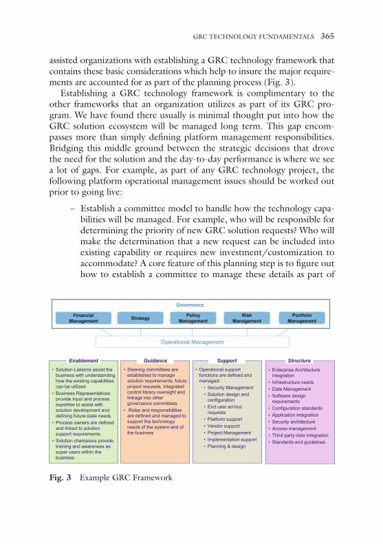
assisted organizations with establishing a GRC technology framework that contains these basic considerations which help to insure the major require-ments are accounted for as part of the planning process (Fig. 3 ).

Establishing a GRC technology framework is complimentary to the other frameworks that an organization utilizes as part of its GRC pro-gram. We have found there usually is minimal thought put into how the GRC solution ecosystem will be managed long term. This gap encom-passes more than simply defi ning platform management responsibilities. Bridging this middle ground between the strategic decisions that drove the need for the solution and the day-to-day performance is where we see a lot of gaps. For example, as part of any GRC technology project, the following platform operational management issues should be worked out prior to going live:

– Establish a committee model to handle how the technology capa-bilities will be managed. For example, who will be responsible for determining the priority of new GRC solution requests? Who will make the determination that a new request can be included into existing capability or requires new investment/customization to accommodate? A core feature of this planning step is to fi gure out how to establish a committee to manage these details as part of

Operational Management

• Solution Liaisons assist the business with understanding how the existing capabilities can be utilized

• Business Representatives provide input and process expertise to assist with solution development and defining future state needs

• Process owners are defined and linked to solution support requirements

• Solution champions provide training and awareness as super users within the business

Enablement• Steering committees are

established to manage solution requirements, future project requests, integratedcontrol library oversight and linkage into other governance committees

• Roles and responsibilities are defined and managed to support the technology needs of the system and of the business

Guidance• Operational support

functions are defined and managed:• Security Management• Solution design and

configuration• End user ad-hoc

requests• Platform support• Vendor support • Project Management• Implementation support• Planning & design

Support

• Enterprise Architecture integration

• Infrastructure needs• Data Management• Software design

requirements• Configuration standards• Application integration• Security architecture• Access management• Third party data integration• Standards and guidelines

Structure

Financial Management Strategy Policy

ManagementRisk

ManagementPortfolio

Management

Governance

Fig. 3 Example GRC Framework


the overall GRC program, where that committee reports into and who is a member of that committee (GRC stakeholders).

– As part of the operational management model, also plan out the roles that will be required to support the technology platform as part of the GRC technology support program. This is normally done in addition to fi guring out who owns the actual GRC tech-nology platform and associated solutions and who will be respon-sible for directly supporting the platform. There are core roles that are required to not only support the technology but also to provide business support for the capabilities as well, such as:

– solution architects; – business analysts; – solution developers; – platform confi guration specialists; – trainers; – BAU support personnel.

– Some of these roles can be performed by the same person, espe-cially as the GRC technology capability is initially developed. However, over time there may be a demand to drive more integra-tion across the enterprise, so these roles will grow in importance. Finding skills in the marketplace that understand technology and business processes related to GRC processes and functions are in big demand.

Integrated Control Library An important element of GRC technology solutions is the utilization of different types of content. In this context, content can mean any of the following types of data:

– controls; – policies; – procedures; – loss events; – threats; – vulnerabilities; – assets (can include processes, information, facilities, software

applications, etc.); – risks;


– regulations; – confi guration data; – key risk metrics; – questionnaires; – other sources of data.

The most commonly used content for GRC technology solutions revolves around controls, risks, and assets.

A control library is critical in order to be able to provide effi ciency and cost savings for automated compliance management tasks. Early forms of GRC use cases for risk and control self-assessments and control test-ing utilized dedicated controls and associated question libraries that were assigned by regulation. For example, PCI-DSS would have a set of con-trols (and corresponding questions for assessment and testing) and corre-sponding support questions just for that regulation. HIPAA, GLBA, and other regulatory requirements would all have their own defi ned control and associated question sets. While this architecture did provide a benefi t over using Excel spreadsheets or doing things manually, it did not address several common challenges such as having to continually produce the same evidence to show compliance with multiple regulatory requirements.

A more effective approach is to use an integrated control library as a master repository of controls. The idea behind the integrated control library is that all controls are harmonized and indexed together, while the dupli-cates are removed from the master library. Using this technique signifi cantly reduces the number of control requirements that have to be used for test-ing while increasing the amount of regulatory coverage an assessment can provide. This integrated control set then would act as the central repository for all control related decisions. For example, if a control is mapped against several requirements, then testing it one time should suffi ce as coverage against all of the requirements that it is mapped against. There are sev-eral prominent IT-focused integrated control libraries in the marketplace that organizations can purchase to add to their GRC technology platforms, such as the Unifi ed Compliance Framework, (UCF). Other sources of inte-grated control libraries can include open source options from some of the standards bodies (ISACA, ISO, FFIEC, etc.) as well as from GRC vendors themselves, consulting organizations, and law fi rms (Fig. 4 ).

There are several design challenges related to how an organization decides to implement an integrated control library. Even if you purchase a library from a third-party vendor, there may still be signifi cant work to adjust the


controls and associated language to the organization’s operational conditions and culture. A common complaint among end users is that regulatory or stan-dard/guidance control language is not easy to understand. Several additional challenges to consider are:

– Design seed for the indexing structure—domain structure lan-guage to use (ISO instead of COBIT, NIST, etc.).

– Mapping to the highest common denominator—if you have PCI as part of your regulatory universe you do not want to map all of your controls to the PCI standard—you may end up over testing things not related to PCI boundaries).

– Jurisdiction requirements—different geographies may require different controls, for example different state laws rules and regulations.

– Standard language used based on particular needs—for example if part of the business requires doing business with the federal government then NIST 800-53 control structure/language may be required, etc.).

– Deciding what to map together—in addition to harmonizing reg-ulatory requirements, do you also include policies and procedures to the control set?

Data Feeds

Internal Controls Standards Third Party Library Policies Other…

Architecture

Feeds can include sources that are internal, Law, Rule and Regulatory specif ic sites, standards bodies, common pract ices, third party providers, law f irms, GRC plat form vendors and various other vendors.

Sources

Requirements

• Control Objective• Control Activity • Test procedure

Solution Details• A base is selected to provide the initial set of domains to build the index, from standards such as ISO, NIST, COBIT or

others• Elements such as geography, business unit, applicability and others are designed into the architecture as support fields• Provides full traceability back to all sources of the requirement

Master index

Risk Domains

Fig. 4 Example of an Integrated Control Library


– Establishing governance around who owns the control set, who is allowed to make changes, and how regulatory changes are made.

One of the important decisions when considering the acquisition of GRC technology platforms is how the control library content will be architected, acquired, implemented, and managed. The marketplace has grown for dedicated content services and organizations have the ability to purchase support services from managed service providers in addition to the sources mentioned above.

Another important consideration for the control library is how to account for risk. Since risks and controls often share a many-to-many rela-tionship (meaning a control can offset many risks and a risk may be linked to many controls), considering how the architecture of risks and controls is designed up front is key to a smooth operating GRC technology system. There are a couple of ways in which risks can be connected to controls within the GRC technology platform.

– As part of the control library. Many organizations that are start-ing out with GRC technology solutions or are fairly immature in their GRC processes elect to host risk domains and risk statements within the integrated control library. In our experience many organizations do not start out having a predefi ned list of risks that apply to business such as IT. Instead, they rely on leveraging the control library and corresponding risks as a starting point to work from.

– Within a dedicated risk register. Establishing a dedicated risk reg-ister enables an easier way of independently utilizing the risk data across different GRC solution capabilities. There is some heavy mapping work that is required to establish the many to many rela-tionships between risks and controls, but once completed the rela-tionships can be maintained within the GRC technology platform.

The discussion of how to architect a support system to contain (enter-prise) risk domains and associated risks is a very important planning detail required before implementing a GRC technology platform. We have wit-nessed many organizations relying on compliance requirements and asso-ciated controls to guide them on the recognition and treatment of risks. This has come to be known as managing risk as a “compliance checklist” exercise. As GRC programs and processes have matured, we see the reliance upon compliance controls used to defi ne risks diminishing as organizational


knowledge and processing capabilities about risks improves. Several other challenges that are related to maintaining risks within a GRC technology platform include:

– Mechanism used to populate risks. For example, many organiza-tions do not utilize the risk assessment process to discover new risks, instead using likelihood and impact calculations to mea-sure how controls are performing (effective). Many risk assess-ments are designed to leverage existing standards, such as ISO or COBIT domains and associated controls (harmonized with regu-latory requirements) which does not provide a means of discov-ering new risks. In order for risk data to be accurate and useful, there needs to be a mechanism designed to discover, maintain, and deactivate risks.

– Ownership of risks. As part of the governance process, establish-ing accountability for who decides something is a risk and who owns the remediation decision-making is also key. Capturing this in a GRC technology platform can be supported through the use of a risk register or repository containing risks.

– Aggregation models. Planning for how risks will be correlated and aggregated is also an important technology design issue that should be handled as part of the overall design process for risks.

– Provide the ability to risk rationalize controls. The basic idea is to enable control decisions based on risk. This would include estab-lishing the ability to risk rate control objectives, perform risk based control testing, and provide a control baseline based on risk levels.

Assets While control and risk data has been the biggest focus for GRC technol-ogy platforms asset data should be considered equally important. The abil-ity to link assets such as processes to risks and controls can provide a big benefi t to many GRC solutions through automation. While asset data is a crucial part of a GRC program, we have not seen a focus on this capa-bility from GRC technology vendors. While GRC technology platforms can typically handle some amount of assets and linkages with risks and controls, we do not see them scaling to compete with larger data ware-houses or confi guration management databases anytime soon.

There are probably a couple reasons for this. It has been our expe-rience that organizations have struggled to get a handle on fully


automating their asset programs, due to the sheer size, investment, and focus required to address the problem. When organizations have made investments into setting up an inventory for their assets, they have used software specifi cally built for that purpose. It may not make sense to replace the investment made into the asset management tool set in order to setup the data into a GRC technology platform. Organizations have also made investments into building data warehouses for this pur-pose. Another reason may be that there is new thinking around adding risk and controls information as attributes to the asset, which resides in the CMDB (confi guration management database). This new approach would change how GRC technology platforms are used and also how data is architected. We will cover this in more detail in the trends sec-tion below.

Risk Management Methodology There are several important aspects related to the risk management meth-odology that should be considered vital as part of the planning stages for implementing a GRC technology platform. While it is always a good idea to have a complete understanding of the entire end-to-end process required for risk management before embarking on an automation project (mentioned in the overview section above), there are a couple of impor-tant elements that can prevent having to do rework later on down the road, such as:

– Establishing consistent risk taxonomy. Having a common defi ni-tion for risk will enable smoother integration once the GRC solu-tions are leveraged across the enterprise.

– Understanding and documenting the risk criteria required. At a bare minimum, there needs to be an understanding of the follow-ing aspects:

• qualitative or quantitative approach to be used; • levels defi ned — how many and what defi nitions of each level; • risk tolerance threshold — understanding at a high level what actions

each level of risk will trigger; • what measurements are to be used to estimate risks, such as sensitiv-

ity, impact, likelihood, and so forth?


– Risk categories. Defi ning high-level risk categories (sometimes also called domains) will assist in almost every aspect of GRC tech-nology enablement.

As an example of why we feel these are important to consider before starting to implement a GRC technology solution, consider setting up a risk assessment process. The minimum you need in order to perform a risk assessment is:

– a set of questions that probe for risky activities; – a workfl ow process to track progress; – a reporting engine to detail the results of the answers.

Even though this is an oversimplifi cation of the risk assessment process, from a technology standpoint, consider the following scenario. If you cre-ate a risk assessment with ten questions, and each question has a risk rating calculation to be performed for likelihood and impact, how much process-ing will be required to process the calculations? What if you now have 50 questions that each requires this type of calculations? What if each one of these questions was linked to the corresponding controls and required a lookup function from the integrated control library? These are the type of details that would be helpful to understand before implementing a GRC platform.

Of course, there are many more risk management-related elements that require dedicated time and attention to make work. We selected these elements because they have a direct impact on many of the use cases for GRC solutions.

Technology Architecture There are many different ways to defi ne what is meant by the word archi-tecture. In this case, we are referring to the underpinnings that support the data, users, and applications that make up the GRC ecosystem. As part of this description of foundational elements, we are specifi cally highlight-ing the ability to link together systems and data in order to get the benefi t from an integrated set of capabilities.

GRC technology vendors have been making signifi cant investments into product capabilities that provide a one-stop shop for solution requirements. The reality is no single GRC system can yet handle all of the requirements of a GRC program. There are simply too many applications and sources of data that already exist within an organization that it is not


practical to migrate them all over into a single platform. On top of this, GRC technology platforms are not yet capable of handling enterprise scale processing requirements. In fact, GRC technology platforms may not be the best option for some of the functions that GRC programs require for support.

There are several elements related to a technology architecture that should be considered up front before implementing a GRC technology platform:

– Processing capability. As part of an overall data architecture, is the GRC technology platform the right system to house the solu-tion and associated data? Is it better to house the data in another system, and just pull what is needed for processing? Will growth of the solution cripple the processing capability of the platform?

– Third-party linkages. How a GRC platform provides the ability to connect with other applications and systems is important for long- term growth of the platform. Considering how the GRC technol-ogy platform aligns within the technical infrastructure will prevent having to redesign the platform or data structure as the solution demand grows.

– User interface. One of the biggest complaints regarding GRC technology platforms we have heard universally involves this ele-ment. We have found that this aspect of the technology platform should be minimized so that only the super users and support staff required to maintain the systems regularly access the user interface. The sooner you can get end users to interact with reports, dash-boards, and homepages the more this element can be minimized.

GRC Technology Platform Selection First a note about technology support for GRC program functions. This chapter is specifi cally about GRC technology platforms but, as mentioned earlier, there are many different technology capabilities that can be lever-aged to support GRC program efforts. Since GRC technology platforms are integrated solutions (database, workfl ow, and reporting) they are a popular choice for supporting GRC programs. However, we have wit-nessed plenty of large organizations design their own tools or utilize tools that support other disciplines or leverage a hybrid of the two that it is worth considering if this is the right path to take.


Before embarking on an exercise to select a GRC technology platform, there are many strategy, process, and culture issues that need to be defi ned. Since this chapter is about GRC technology, we are going to be focused on starting from the perspective that the decision has already been made to acquire a GRC technology platform. There are several core issues that should be examined before getting into the process of how to evaluate a GRC technology platform. These are what we call the “framing” elements since they start to defi ne the core requirements needed to frame the chal-lenge that the GRC platform will be involved in addressing:

– Culture . Not considering all of the impacts that GRC process improvement, integration, and automation will create is the single biggest reason for failure we have seen related to GRC projects. Becoming more effi cient (and integrated) with tasks related to GRC tends to break down and expose siloes of decision-making and ineffi ciencies.

– Scope . Deciding how big of a change to make regarding GRC processes should be considered before starting down the path toward automation. Sometimes it is much easier to start with small changes that impact a very limited part of the business and grow from there. It is not often we see enterprise-wide challenges tackled as a fi rst step toward gaining effi ciencies and cost savings.

– Processing location . This variable revolves around whether the Cloud or SaaS (software as a service) can be leveraged or if the technology has to be utilized on premise (or a hybrid between on-premise and cloud). This consideration may direct the solution review in a different direction since not all vendors support cloud implementations. One of the biggest criteria for consideration is whether there is trust that important and sensitive data used in the processing of GRC solutions and reports will not be exposed in a cloud-based solution.

– Strategy . Understanding the big picture end goal should be defi ned before starting down the path for any GRC process improvement project. Not understanding how to integrate GRC programs for the betterment of the organizational operating model may cause a lot of additional work to be performed down the road.

These framing elements will help start the planning process that can be used to select the right technology platform to address the defi ned issues.


Clearly understanding the scope of the challenge, the people impacted by the challenge, how addressing the challenge fi ts into the overall goals of the organization, and what type of solution may be required to address the challenge is a good starting point for planning.

Planning to acquire a GRC technology platform can seem like a daunting task. There are so many different GRC vendors with various solution options that it can make the decision to select a technology platform diffi cult. With so many options available it is vital to perform a couple of planning steps to help narrow down the choices.

The fi rst step for planning to automate a GRC program function is to defi ne your requirements. It is vital that the issues that are driving the need to implement a GRC technology platform are defi ned and docu-mented. Requirements can be divided into several different sections:

– General requirements. These are used to defi ne any core consid-erations that the GRC vendor will need to address that are not specifi c to a solution. Considerations such as cost, vendor refer-ences, external consulting services, support network, and vendor product roadmap (among others) can be defi ned in this section.

– Functional requirements. The core requirements related to defi n-ing the challenges being addressed by the GRC technology platform.

– Support requirements. Sometimes referred to as non-functional requirements, these usually defi ne the support needs of the envi-ronment that the platform is going to be running.

In order to defi ne the requirements, organizations may want to solicit feedback from stakeholders that were defi ned as part of the framing elements exercise. The requirements should be agreed to before the selection process begins so that all considerations have been vetted and documented. This same stakeholder group may then be used as part of the selection process. Another element that may be needed is to rate the importance of the requirement itself so that there can be a weighting of the importance of the criteria. Since it is unlikely that a vendor will be a perfect match to every requirement, it may help if the stakeholders can agree on which requirements are “must haves” and which ones are just nice to have. Vendors that do not meet all of the “must have” require-ments then do not move on to the next phase of assessment.


Now that requirements have been defi ned, it is time to select a few vendors for consideration. We have watched organizations use the follow-ing vendor selection approaches over the years:

– Rely upon analyst reviews and charts in order to narrow down the fi eld to a select few vendors. Things like the Gartner Magic Quadrant and Forrester Wave have been extensively relied upon by many organizations to help select vendors for consideration.

– Talk to peers and see who they use to address problems that are similar.

– Speak to consultants to see who they recommend should be considered.

– Perform general research by attending conferences, reading arti-cles and reviews and vendor website crawls.

Each one of these methods has its strengths and weaknesses, but several of these methods taken together can get the organization started with a good cross section of vendors to review. It is also important to understand the pedigree of the GRC platform vendors. Some of the GRC platform vendors started out addressing problems with data quality, some of them were strictly focused on SOX (Sarbanes-Oxley), and still others were built with a different use case in mind. Each vendor may have a particular slant based on the type of problems they were originally created to address that will infl uence their ability to expand into support for other solutions. Once the vendors are selected, the method to engage them for evaluation needs to be defi ned.

Engaging the vendors to evaluate product capabilities is the most important step in the process. No matter how the vendors were invited to participate in the next phase, it is critical that each vendor be put through a review process that is fair and represents the capabilities that will ensure the challenges identifi ed in the requirements are actually met in a satisfac-tory manner. During this step, we have seen two approaches used:

– Draft and distribute an RFI/RFP. Depending on the purchas-ing process with the organization, a request for information or a request of proposal may be formally required in order to solicit vendor responses. Appendix B contains an example of a GRC RFP.

– Draft and utilize use cases in order to judge the vendor capabili-ties. This step skips the RFP process and goes right to the vendor demonstration phase.


If the organization requires a formal RFP to be used, then there will need to be a response rating system in place to decide who can go on to the demonstration phase and who is excluded. The advantage of using an RFP is that it will help cast a wider net for vendor responses, and can eliminate any vendors that do not meet the minimum requirements. The disadvantage to an RFP is the extra work required to draft it, set up the rating system, and handle responses for the vendors that do not get invited to the next phase.

The RFP is usually written with a section that describes the criteria that the vendors will be required to fulfi ll in order to make the next phase. The next phase, which is a demonstration of the vendor’s capabilities, is what the RFP is geared towards. While we have seen the RFP process used to select a vendor without a product demonstration, it is far more common to have the vendors perform a demonstration of their capabilities after suc-cessfully meeting the RFP criteria. The other potential process a vendor may be asked to perform as part of the RFP process is an oral presentation. The criteria used to judge a vendor’s response to the RFP can cover a lot of different elements, but usually contains the following:

– GRC vendor’s record of performance and service in organiza-tion’s industry;

– GRC vendor’s conformance to RFP’s specifi cations, require-ments, terms, conditions, and provisions;

– extent of GRC vendor’s experience, stability, supporting resources, and management;

– cost of products to be purchased—examine the total cost of ownership;

– innovative offering and solutions to further enhance the partnership;

– GRC vendor’s fi nancial stability and references.

Keep in mind these are criteria for evaluating an RFP response—not just adherence to the requirements. Many organizations that have deployed GRC technology took the steps to have the vendors perform a presenta-tion to explain their RFP response in more detail and also to perform a live demonstration of their capabilities.

As part of the RFP process organizations may have the vendor send a team of people to meet and discuss the response. We have seen organiza-tions use this meeting in order to get a feel for the vendor’s personnel, its culture, and form an overall impression. RFP responses can be very labor


intensive to craft responses, especially if the RFP is heavily customized toward an organization’s particular challenges. This meeting provides the vendor to get a feel for the context of the RFP requirements, as well as some of the stakeholders they may be working with on the project. This meeting may also give the vendor the chance for any clarifi cations which may help it formulate its strategy when it comes time for the live product demonstration.

A fi nal step in the vendor selection process involves the live demonstra-tion. A common approach is to whittle down the original RFP responses to the best three or so vendors and then invite them to demonstrate their capabilities (a.k.a. the bake-off). This step provides the vendor with the opportunity to show how their platform capabilities can meet or exceed the requirements that have been laid out in the RFP. Based on our expe-rience, we would recommend this is where to craft a small subset of use cases that the vendors need to utilize to showcase their capabilities. We have found it is very diffi cult to get a good understanding of the complexi-ties and differences between the vendor platforms if the demonstrations are left up to the vendors to showcase their best capabilities.

The use case approach can be used to test a range of capabilities that the vendors can provide. Using this method enables the requirements to be directly linked back to their use case narratives for the sake of coverage for the demonstrations. This method will help the evaluators understand if a capability is native to the platform, “out of the box”, requires slight modifi cations (confi guration), or something more involved through cus-tomization. As part of the use case design, we would recommend that a script is developed which highlights the expectations of the demonstra-tion, a description of the use case, a sample data set to be used for the use case, and steps to be performed for the use case. Providing this level of detail will enable a fair comparison of the likes and dislikes of the vendor platforms being considered, along with potential costs of the solution and any potential customization efforts. Most user demos we have participated in have run on average about three hours. We have seen demonstrations go as fast as one hour or run for as long as ten hours.

One of the challenges of examining GRC technology platforms using capabilities in a use case narrative is that it does not necessarily take into account how the technology can handle integration across processes, content, and technology architecture. Instead of comparing features and functions of the GRC technology platforms head to head, more emphasis should be placed on how well each platform can handle capabilities that


enable integration between the functions. In fact, when we have assisted clients in vendor technology selection, we have included this integration capability as an additional part of the use cases. This forces the vendors to showcase not only what level of capabilities can be natively provided but also how their software platforms would potentially function using capa-bilities that may not be “out of the box”. Examples of some integrated capabilities to add to use cases include:

– integrated control library (actual harmonized controls); – third-party data integration; – risk aggregation models; – many-to-many linkages between integrated controls and risk

register; – linkages between assets, risks, and integrated controls; – establishment of risk rationalized control baselines (collection of

controls based on risk rating for a specifi c type of asset).

Once all of the vendor demonstrations have been completed, the fi nal scores can be compiled. Organizations have used multiple ways to score vendors throughout this process, but two methods tend to be more com-mon. Vendors can be scored on the RFP items mentioned above, which includes scoring the vendor demonstration as a part of the overall RFP score. Organizations have also used a technique that uses one scoring sys-tem to evaluate the vendors in order to get to the demonstration phase, and then a completely fresh set of scoring metrics to rate the vendors on their demonstration of capabilities. The score for the vendor demonstra-tions would be the fi nal score for determining which vendor is selected.

In order to properly evaluate the vendors and insure a fair process, scoring metrics need to be established and clearly articulated to all parties. Decisions need to be made about the following parameters:

– Weighting . Some requirements are more important, and thus carry more weight than others. Organizations have used weight-ing to highlight those requirements or requirement areas that matter more in the scoring criteria.

– Work effort . Some organizations have set up a separate scoring system to measure how complex a requirement may be to imple-ment. Organizations that want to stay focused on as much “out of the box” functionality as possible can use this metric to show where a requirement may need more effort to automate.


– Scale. It is common to see a scale of sero to fi ve or one to fi ve used as the basis to rate the parameters. For example, if a requirement is weighted as a four or higher and receives a zero on one of the requirements, it would be automatically disqualifi ed (meaning it would fail to meet an important requirement).

– Aggregation . Need to determination which criteria scores should be included into the fi nal calculation of the vendor capabilities.

An example of this type of scoring system is as follows (Table 1 ): There are several additional factors to consider when planning to acquire GRC technology such as:

– A single enterprise platform . As mentioned at the beginning of this section, there may not be a single “best” platform to address all of the challenges that are required to be automated. It is rare to see an enterprise GRC program automated with a single technol-ogy platform. They simply are not mature enough in their solution offering breadth and depth to cover all of the enterprise needs.

– The leveraging of existing technology. There may be technol-ogy capabilities already in use that can be leveraged to provide the capabilities required to support the GRC program challenges. For example, many organizations have not utilized a GRC technology

Table 1 Example vendor scoring system Overall scoring summary Category Vendor

A Vendor B

Vendor C

Relative weight

Vendor A weighted score

Vendor B weighted score

Vendor C weighted score

1. Functional Requirements (60%)

3.37 3.44 3.31 0.42 1.42 1.44 1.39

Technology (10%) 3.72 3.53 3.81 0.07 0.26 0.25 0.27 Support (10%) 4.00 4.00 4.00 0.07 0.28 0.28 0.28 Cost (5%) 1.00 2.00 3.00 0.04 0.04 0.08 0.12 2. Customer References (10%)

2.05 1.97 2.03 0.10 0.21 0.20 0.20

3. Use Vase Demonstrations (30% of total)

3.17 2.81 3.21 0.30 0.95 0.84 0.96

Total * * * 1.00 3.15 3.09 3.22


platform to automate the policy management lifecycle due to user licensing costs or other architecture-related issues, and instead have use other capabilities such as web technology (intranets), or other means and simply linked into a GRC technology platform where required.

– Skills of the support team. This consideration may drive some of the decision-making when considering the framing elements (cloud versus on-premise) but should not be overlooked when considering the type of customizations and integration work that will be performed. In addition to the technology support skills, business liaison and process subject matter expertise should also be examined to insure proper coverage. Where there is a skill set gap, external fi rms may be able to augment those skills that are needed.

– Strategy/direction of the IT organization . This may also be considered as part of the framing elements for planning purposes (cloud, SaaS, etc.) but also can impact platform capabilities in the future. For example, we have seen organizations purchase an on- premise GRC platform, and right in the middle of the implementa-tion process make a wholesale change to cloud-based applications.

– Future needs . The importance of this consideration cannot be overstated. We have witnessed many organizations undertake silo GRC process improvements without the ability to come together and link efforts into a more integrated approach. Many organiza-tions have acquired multiple GRC technology platforms due to this type of problem-solving process, which then creates its own share of content and workfl ow challenges.

– Maturity level . It may sound like preaching, but how many times have you heard a story of an organization that bought a GRC platform fi rst and then tried to adjust its processes and functions as part of the tool implementation process. It goes without saying that a lot of effort should go into understanding the specifi cs of the issues that need to be addressed, where integration can be cap-tured and the respective content and other foundational elements can be designed and leveraged before attempting to automate.

– Appetite for external assistance. Acquiring additional assistance can come in several forms, such as from the vendor, a consulting fi rm, or another third party that can provide insight into the pro-cesses or technology being utilized. Since the authors have been


on both sides of the equation (purchased services and provided services) our opinion may be biased more toward the value pro-vided by consultants, but as a general rule of thumb:

• Vendors services: The GRC vendors have people who are very knowledgeable about their specifi c product capabilities. Over time, as more clients implement their capabilities to enable more solutions, their experience level grows across industries and solution categories. Generally speaking, the GRC vendors are strong on their product but weaker on industry knowledge and processes, GRC program functions and the associated integration benefi ts that can be derived.

• Consulting fi rms. Basically, almost the complete opposite of the vendors. Most consulting fi rms are deep on industry knowledge and support processes, GRC program functions and tasks, but weaker on the technology support capabilities. Over time, similar to vendor services teams, consulting fi rms build up architecture and techni-cal expertise by industry that can be invaluable. The marketplace demand for GRC automation capabilities is so fi erce that keeping these skill sets for a long period of time can be challenging. Some consulting fi rms are more generalists and attempt to provide support for a wide range of tools, while others specialize in only a handful of tools.

• Miscellaneous third parties. There are many other types of fi rms such as law fi rms, market analyst fi rms, and specialists that may be able to provide targeted assistance or specialized services tailored to a particular need.

It is not uncommon to fi nd that organizations have had to acquire addi-tional GRC technologies due to overlooking some of these factors. In some cases, we have also witnessed organizations that have chosen to completely start over due to the myriad problems that arose related to the choice of a particular GRC technology platform and/or implementation/support part-ner. Typically, multiple tools end up within the same organization due to cultural/political challenges and not due to technical limitations.

GRC Technology Challenges and Future Trends Each year there are predictions for the hottest trends and GRC challenges where organizations will focus their time and attention. For the most part,


there are similar themes observed almost every year these types of predic-tions are made. For example, in 2007 some of the trends that were noted for GRC were identifi ed as:

– technology will continue to evolve and mature; – entrance into the marketplace of software heavyweights; – a GRC ecosystem will develop; – risk and regulatory intelligence will improve.

Many of these predictions still hold true today. Instead of using this section to discuss upcoming trends along these lines, we wanted to point out where we see organizations trying to drive vendors to make changes or where we think inevitably the changes will need to occur. There are two primary ways we are collecting information to make these observa-tions: through tracking marketplace investments and direct involvement, witnessing organizational maturity with various GRC solutions through our exposure to GRC projects and client issues.

From a growth perspective, by many analyst accounts the GRC tech-nology marketplace is doing very well. While there are many analysts now providing revenue projects for the GRC technology marketplace, conservative estimates place the revenue growth to be 9–14%, with rev-enue climbing to reach upwards of $30 billion by 2020 (depending on how the analyst is defi ning which solutions make up the GRC market-place). This type of growth tends to drive a very active vendor mar-ketplace, with mergers and acquisitions and investment into expanding capabilities.

GRC vendor mergers and acquisitions have been very active over the years as companies attempt to expand market reach and broaden their technical capabilities. Some notable acquisitions include the following:

– IBM’s acquisition of OpenPages, Algorythmics, and BigFix; – New Mountain Capital’s acquisition of ACA Compliance Group; – First American Financial’s acquisition of Interthinx, Inc. – Wipro’s acquisition of Opus CMC; – Goldman Sachs’ investment into MetricStream; – Wolters Kluwer acquiring Effacts Legal Management software,

Datacert, SureTax, Learner’s Digest, and LexisNexis legal busi-ness in Poland;

– EMC acquiring Archer Technologies, Netwitness, and Symplifi ed Technology


– Thomson Reuters acquiring Paisley, Complinet, World-Check, and WeComply;

– Nasdaq OMX acquiring BWise.

Investment into expanding capabilities is also a good barometer of the health of the vendors in the marketplace. This can be seen in two major activities. First, established GRC technology vendors continue to expand their product capabilities as clients demand a more mature product offer-ing. Second, vendors that may only partially be in the space can decide to add core GRC support capabilities to provide a growth avenue for their existing clients. We have seen this with vendors in the business process management (BPM), helpdesk, asset management, and business intelli-gence spaces lately.

From an established GRC vendor perspective, gaining insight into the prod-uct roadmap can provide a good view of where capabilities will be improved. Since vendors have slightly different core strengths, their future state product roadmap provides one view of where GRC capabilities are heading.

From an organizational perspective, as GRC processes and models mature and improve, new requirements naturally emerge. One of the big-gest impacts is leveraging the integration capabilities gained through GRC process improvement and technology support. For example, establishing a harmonized set of controls, having them risk-rationalized and linked to assets is a common starting point for many GRC projects. Enabling this fundamental capability provides many new opportunities for leverage into other solutions. Functions such as business continuity, vendor risk man-agement, and threat and vulnerability management can all benefi t from this integrated capability. As we see organizations improve in this manner, a new set of challenges arises for even more visibility and integration across the enterprise. Some of these new areas of improvement include security analytics, asset management, big data, and security operations functions.

Security analytics as a solution has been around for some time. As data sets for risks, controls, and assets have become more accurate and better aligned, indicators and metrics via key risk monitoring solutions have also improved. As all of this information becomes more accessible, accurate, and timely, the demand for analytics is a natural manifestation of these maturing processes. In fact, in our opinion the GRC marketplace will slowly evolve into which vendor can provide the best analytics solution once all of these GRC processes and data sets are fully integrated. It is ultimately where the solution capabilities all lead.


Another change we are witnessing involves asset management. In the traditional solution, asset management provides an organization with the ability to acquire, deploy, operate, and dispose of assets cost-effectively. What we are seeing is the merger of this process into GRC, so that risks and controls are becoming attributes of the asset. This is a very different means of managing risk and compliance than has been done in the past, but is consistent with how IT organizations have been managing their operations. We have seen very large organizations start to realize that they need to have a solid asset foundation in place in order for the improve-ments related to risks and controls to be fully realized.

One of the solutions that we are seeing mentioned with more frequency is the movement to involve “big data”. While it is true that GRC becomes a data warehouse challenge over time as the use of solutions increases, one of the ways we have seen organizations handle this capability is via the asset management solution. In addition to asset inventories containing attributes for ownership, risk, and control details is the requirement to pull together all different types of data. A big data solution lends itself to this type of requirement.

Integrated security operation is starting to become a reality as more information and processes become interconnected. We are starting to see organizations taking their threat and vulnerability information and con-necting it with their assets and associated risks and controls. There are several methods that have been around for a while that assist organizations with combining threat and vulnerability information into a scoring model, for example, but the newer approaches are pushing the boundaries to link up much more information that can provide better visibility into risks. Threats, vulnerabilities, assets, controls, risks, internal security systems log data, internal audit fi ndings, loss data, fraud information, and a host of other data can now be correlated and aggregated to produce exposure factor, appetite, and posture levels. An example depiction of this capability is as follows (Fig. 5 ):

GRC technology platforms face several challenges as organizations try to address enterprise business needs. As challenges do exist with the peo-ple and process components of GRC, we will only be covering some of the common challenges we see related to GRC technology platforms in this chapter. Many organizations need to consider the functions that may be better served by not being natively housed in a GRC technology platform. There are many approaches that can provide increased value through an integrated architecture approach, rather than trying to shoehorn func-


tions and processing into a platform that may not be capable of support. We have broken down the GRC platform challenges into the following categories:

– Scalability . Many of the GRC technology products were designed to be used to solve specifi c problems, and have increased capabilities over time. Within this topic there can be challenges with process-ing large amounts of users and associated tasks. While some of the enterprise class tools such as ERP have added GRC capabilities and do not necessarily face this problem, many of the platforms that grew up addressing IT GRC or other specifi c GRC- related chal-lenges may have enterprise limitations around users and processing.

– Solution coverage . There are two components to this weakness. First, traditional GRC platforms may not be ready to support enterprise level demands for solutions as they have not matured enough yet to provide all the necessary coverage. Secondly, the GRC platforms that do provide a good deal of the capabilities required to support the enterprise may not be architected to sup-port the integration requirements that GRC drives.

– Data storage . Generally speaking, GRC technology platforms were not designed to be data warehouses or confi guration man-agement databases (CMDB). GRC vendors have provided some

GovernanceRisk Management Methodology

Foundat ional data repositories

Risk Register IntegratedControls Assets Threats Policies &

ProceduresMetrics Configurations

Inputs from program function Assessments

Audits

Control Testing

Incident Response

Remediation Plans

Security Analyt ics / Report ing


Enterprise use Cases

Policy Management


Education & Awareness

Internal Audit Business Continuity Management

Incident Management Asset Management

Data Feeds:• Threats• Vulnerabilities• Loss events• Internal fraud

Security Tools:• IDS / IPS• DLP• NAD• IAM• SIEM• Virus / Malware

Technology Plat forms (GRC / Monitoring / etc.)

Workf low Support

Fig. 5 Example GRC Integrated Architecture


support for asset inventory and classifi cation capabilities, but for large-scale deployments GRC technology platforms may not be the right choice yet.

– User Interface . This is one area where GRC vendors are con-stantly working to improve the end user experience using their software. Since this element is in the eye of the beholder, what may be a weakness for one stakeholder may be a strength for another. One of the interesting side notes to this consideration is that we have seen organizations starting to worry less about what software the business is using to collect information and more focused on making sure things on the back end are processing correctly. Many of the GRC tool consolidation projects we have seen have been driving a reduction for back-end processing more than at the business level for things like performing assessments or control testing.

– Document management . As with data storage, many of the GRC technology platforms were not designed to be large document management systems. GRC vendors do provide the ability to do some document management capabilities, but if you need to store large amounts of data, such as control test results and associated evidence fi les, another system may be better suited to handle the capabilities through a linkage. There are other document man-agement features typically found in dedicated software, such as check-in/check-out capabilities that may not be in some of the GRC technology platforms.

No technology platform is perfect. GRC technology platforms have come a long way over the past decade in enabling real value to be realized.

APPENDIX A: PARTIAL REQUIREMENTS EXAMPLE

Functional Requirements

Enterprise Risk Management • Support for objectives

– Process to manage objectives – Reporting and monitoring of progress


• Establish risk register – Support architecture for fi ve domain levels of risk – Minimally support capabilities to track:

• Risk ID • Risk owner • Risk Description • Risk Domain • Linkage to controls, policies, and assets • Ability to track remediation

– Ability to aggregate risks – Ability to prioritize risks – Ability to support different methods to link risks to fi nancial loss

amounts • Risk Management

– Establishment of common terms for risk elements – Support for different risk measurement criteria

• Organizational Structure – Ability to support multiple levels for an organizational structure – Ability to support changes to the organizational structure via drag

and drop capabilities

Operational Risk Management • Same requirements described in the ERM section above plus: • Loss Events

– Ability to support loss event data – Ability to support the exportation of loss event data – Ability to support anonymizing key elements of the exported loss

event data

• Scenario Analysis – Supports storage of customized scenarios – Supports data import for use in scenario analysis – Supports what if scenarios as part of scenario analysis process – Support different measurement calculations as part of scenario

analysis

• Integration capabilities with other operational risk programs such as BCP, vendor, and IT Security

Policy Management • Structure for lifecycle process


– Supports a policy library (examples) – Support for importing/exporting policies and procedures – Supports multi-tiered approval process for creating new policies – Support for tracking policy versions – Supports workfl ow and approval process for policy revisions – Ability to archive policies – Identify and highlight/rate most viewed or searched policies

• Exception Process – Supports policy exception requests – Supports exception request review and approval workfl ow – Provides updates regarding the termination of exception period

• Workfl ow – Supports distribution based on user roles or other criteria – Ability to support issuing surveys to end users based on policy

content – Ability to distribute policy content based on dates

• Awareness – Ability to track who has read a policy – Ability to provide tests on policy content – Ability to notify users when testing is required – Ability to track testing results

Risk Management • Supports risk assessment process and associated workfl ow • Supports alternate risk measure approaches

– Qualitative/quantitative/hybrid risk measurement – Ability to control level of control user is given over risk calculation

parameters and weights – Support for threat/vulnerability measurement approach to risk

assessme nt • Supports standards-based dollar quantifi cation of risk

– Single occurrence loss expectancy (SLE) – Annual average loss expectancy (ALE) – Annual rate of occurrence (ARO) – Supports standards risk assessment methodologies and algorithms – Supports custom risk assessment methodologies and algorithms – Supports survey campaigns based on date or other automated

milestones


– Supports tracking of corporate directives and the extent to which potential risks may impact them

• Mitigation and Remediation – Support for multiple risk responses including:

• Acceptance • Avoidance • Deviation • Mitigation

– Supports cost and “what if” analysis of mitigation options – Supports problem ticket creation, notifi cation, workfl ow, resolu-

tion tracking – Supports routing of fi ndings to the appropriate personnel – Supports integration with external trouble ticket/incident man-

agement solutions • Supports common control frameworks for IT risk and compliance,

including:

– ISO 27000 – COBIT – NIST 800-53

• Supports integration of measurements captured from third-party tools: – Vulnerability scanners – Threat data – Security confi gurations – Asset management (CMDB) – Business impact analysis

Compliance Management • Support for using survey-based and automated-testing results and

data from third-party tools • Supports calculating compliance scores for each regulation • Supports aggregation of scores for various regulations • Supports communication to testers and stakeholders of their tasks

through email notifi cations • Support for reporting and dashboard capabilities

Workfl ow • Supports document management capabilities • Supports unlimited workfl ow steps


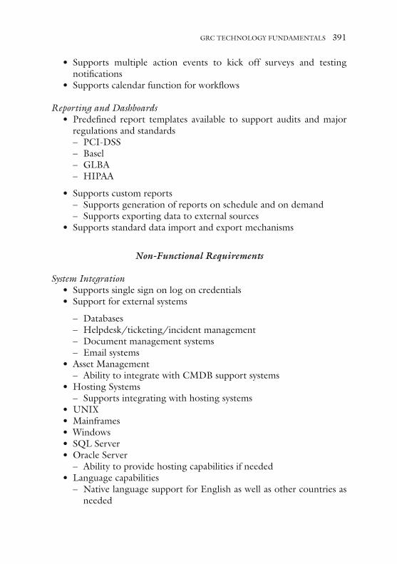
• Supports multiple action events to kick off surveys and testing notifi cations

• Supports calendar function for workfl ows

Reporting and Dashboards • Predefi ned report templates available to support audits and major

regulations and standards – PCI-DSS – Basel – GLBA – HIPAA

• Supports custom reports – Supports generation of reports on schedule and on demand – Supports exporting data to external sources

• Supports standard data import and export mechanisms

Non-Functional Requirements

System Integration • Supports single sign on log on credentials • Support for external systems

– Databases – Helpdesk/ticketing/incident management – Document management systems – Email systems

• Asset Management – Ability to integrate with CMDB support systems

• Hosting Systems – Supports integrating with hosting systems

• UNIX • Mainframes • Windows • SQL Server • Oracle Server

– Ability to provide hosting capabilities if needed • Language capabilities

– Native language support for English as well as other countries as needed


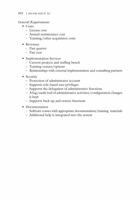
General Requirements • Costs

– License cost – Annual maintenance cost – Training/other acquisition costs

• Revenues – Past quarter – Past year

• Implementation Services – Current projects and staffi ng bench – Training venues/options – Relationships with external implementation and consulting partners

• Security – Protection of administrator account – Supports role-based user privileges – Supports the delegation of administrative functions – A log/audit trail of administrative activities/confi guration changes

is kept – Supports back-up and restore functions

• Documentation – Software comes with appropriate documentation/training materials – Additional help is integrated into the system


Risk Management: Challenge and Future Directions


Quantitative Finance in the Post Crisis Financial Environment

Kevin D. Oden

K.D. Oden (*) Wells Fargo & Co., San Francisco, CA, USA

The views expressed in this document are the author’s and do not reflect Wells Fargo’s opinion or recommendations.

IntroductIon

Mathematics is a disciplined approach to solving problems. As a byproduct of that approach, beautiful truths are often discovered, problems some-times solved, and these beautiful truths and sometimes solved problems usually lead to even more interesting problems.

Finance has historically been rich in problems to solve:

• portfolio optimization;• investment strategy;• performance analysis;• estimating fair value;• price prediction.

From attempting to solve these financial problems, many beautiful “truths” have been discovered:

396

• mean-variance analysis;• factor modeling and arbitrage pricing theory;• performance ratios;• risk neutral pricing;• and more recently, market microstructure theory.

So far most studies in mathematical finance cover material to understand and analyze these mostly “classical” financial problems, with most putting a strong emphasis on the risk neutral pricing of derivatives. Though these prob-lems remain an important aspect of quantitative risk management for banking organizations around the globe, the financial crisis brought to the forefront many old problems that now needed to be viewed in the light of a new finan-cial environment, exposing flaws in how these problems where traditionally approached. Furthermore, the crisis raised new issues that required quantita-tive analysis and potentially a new set of tools to perform theses analyses.

In the next sections we will briefly explore the quantitative problems associated with five risk areas: the fair value of credit, debt, funding and capital risk, collectively known as XVA risk; operational risk, fair lending risk, financial crimes risk, and finally model risk. The problems analyzed fall both in the category of “old with exposed flaws” as well as “new and in search of new tools”. However, each of these topics is worthy of a book in its own right, so by design we cannot delve deeply into any one of them, but provide relevant references for the reader to continue her research. Finally, we note that this is not intended as a comprehensive list of all of the quantitative problems facing the industry today. But in many respects these quantitative problems have emerged post-crisis and have found themselves on the top of many firm and regulatory agendas.

the FaIr Value oF credIt, debt, FundIng, and capItal rIsk (XVa)

Credit has always been one of the largest exposures for commercial banks. And even prior to the financial crisis derivative traders at commercial banks realized that all derivative counterparties were not created equally from a credit perspective. The credit quality of the derivative counterparty should be taken into account either through collateral arrangements or through reserving a portion of expected profit on transactions with counterparties. These adjustments to the value of the contract were made to compensate for the possibility the counterparty defaulted before expiry of the trans-action and the costs associated with replacing or offsetting the risk. The

K.D. ODEN

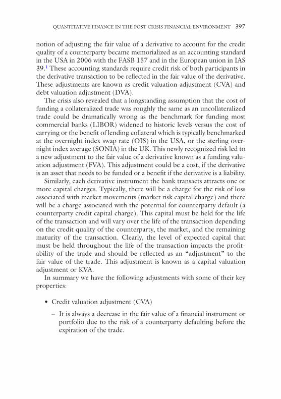
notion of adjusting the fair value of a derivative to account for the credit quality of a counterparty became memorialized as an accounting standard in the USA in 2006 with the FASB 157 and in the European union in IAS 39.1 These accounting standards require credit risk of both participants in the derivative transaction to be reflected in the fair value of the derivative. These adjustments are known as credit valuation adjustment (CVA) and debt valuation adjustment (DVA).

The crisis also revealed that a longstanding assumption that the cost of funding a collateralized trade was roughly the same as an uncollateralized trade could be dramatically wrong as the benchmark for funding most commercial banks (LIBOR) widened to historic levels versus the cost of carrying or the benefit of lending collateral which is typically benchmarked at the overnight index swap rate (OIS) in the USA, or the sterling over-night index average (SONIA) in the UK. This newly recognized risk led to a new adjustment to the fair value of a derivative known as a funding valu-ation adjustment (FVA). This adjustment could be a cost, if the derivative is an asset that needs to be funded or a benefit if the derivative is a liability.

Similarly, each derivative instrument the bank transacts attracts one or more capital charges. Typically, there will be a charge for the risk of loss associated with market movements (market risk capital charge) and there will be a charge associated with the potential for counterparty default (a counterparty credit capital charge). This capital must be held for the life of the transaction and will vary over the life of the transaction depending on the credit quality of the counterparty, the market, and the remaining maturity of the transaction. Clearly, the level of expected capital that must be held throughout the life of the transaction impacts the profit-ability of the trade and should be reflected as an “adjustment” to the fair value of the trade. This adjustment is known as a capital valuation adjustment or KVA.

In summary we have the following adjustments with some of their key properties:

• Credit valuation adjustment (CVA)

– It is always a decrease in the fair value of a financial instrument or portfolio due to the risk of a counterparty defaulting before the expiration of the trade.

QUANTITATIVE FINANCE IN THE POST CRISIS FINANCIAL ENVIRONMENT 397

398

– An increase in credit risk of the counterparty results in a decrease in fair value.

– To hedge this risk requires a hedge of the market exposure as well as the credit exposure. Whereas a credit default swap (CDS) can hedge the credit quality of a counterparty for a fixed notional, the fair value of a derivative portfolio changes with the changes in the underlying mar-ket value (s) driving the derivative. Hence hedging CVA would require a contingent (upon the fair value of the derivative) CDS or a CCDS.

• Debt valuation adjustment (DVA)

– The increase in fair value of a financial instrument or portfolio due to the commercial bank’s (own entity’s) risk of defaulting.

– An increase in risk results in an increase in the fair value. – The increase in the likelihood of default of the commercial bank,

implies an increase in the likelihood it will not have to pay all or some of its outstanding or potential liabilities. Though counterin-tuitive, from an accounting perspective this is a net benefit to the commercial bank.

– Though a net benefit, DVA leads to profit and loss volatility as changes in market factors and the change in the credit quality of the commercial bank changes the value of DVA. Hedging this risk is difficult because most banks will or cannot buy credit protection on themselves. Therefore, typically hedging this exposure is done through buying or selling credit protection on a basket of names highly correlated with the credit risk of the bank.

• Funding valuation adjustment (FVA)

– The cost (benefit) from borrowing (lending) the shortfall (excess) cash from daily derivatives operations.

– FVA can be a either a cost or benefit to the commercial bank. – A derivative asset or one that has a net positive fair value to the

bank needs to be funded.2 Similarly a derivative liability benefits from the bank’s investment rate of return. But the funding and investing rates will differ from bank to bank. From a theoretical perspective, this brings up the question of should FVA be even considered a true adjustment to the price of a derivative since its inclusion breaks the rule of one price.

• Capital valuation adjustment (KVA)

– The expected cost of capital associated with the derivative over the life of the trade.

K.D. ODEN

– KVA is a random variable depending on the anticipated future fair value of the derivative and the present value of the capital associ-ated with the derivative.

The ideas behind these concepts are relatively straightforward. However, they are surprisingly difficult to implement in practice. We describe their calculation a little further in the following and outline some of the practi-cal difficulties.

If we define VR to be the default free and capital free price of an asset and let V denote the default risky price of the asset adjusted for the cost of capital, then one can write

V V CVA DVA FVA KVAR= − + ± −

In particular, if the buyer and the seller of the derivative agree on their respective risk of default (or credit spread) than there is an arbitrage free “price” agreed on by both parties, V :

V = − +V CVA DVAR

However, FVA can be a cost or benefit and more importantly depends on the funding costs of the holder of the derivative and therefore apparently breaks the single price paradigm of arbitrage-free pricing. Furthermore KVA also depends on the capital requirements of a particular bank which, among other things, could depend on the bank’s resident jurisdiction, as well as its size and level of sophistication.

To give some idea of the complexity of accurately calculating each of these adjustments, we observe that CVA and DVA will require the estima-tion of the counterparty’s and the bank’s credit quality throughout the life of transaction, the correlation between these two and their correlation with underlying market risk factors. In order to estimate FVA and KVA we will need to know the cost of funding the derivative and the capital throughout the life of the transaction. See [16] for a good treatment of XVA risk generally and plenty of references.

Except for CVA and DVA, how these adjustments should impact the fair value of the derivative is an open debate in the academic world as well as the accounting world. However, in the industry, whether accounted for in the fair value of the derivative or not, there is a growing realization that there are risks associated with each of these that must be managed as they certainly impact the economic value of the derivatives portfolio.


400

In summary, we can say the fair (or economic) value of an instrument is impacted by the non-performance risk of the counterparty (CVA), the legal entity’s own credit risk (DVA), as well as the cost or benefit of fund-ing the instrument (FVA) and the opportunity cost of capital associated with holding or selling the instrument (KVA). Each of the adjustment concepts is relatively easy to grasp. Yet, even in isolation each can be a dif-ficult quantity to compute, depending on forward implied credit spreads, underlying market risk factors and their implied correlations, to list just a few of the driving factors. These complications alone will provide a fruit-ful source of research for quantitative financial researchers for years to come (see [17]).

operatIonal rIsk

The original Basel Accord set aside capital requirements for credit and market risk. Losses associated with operational failures or the legal fall-out that followed were mostly associated with failures in credit processes or market risk management lapses. But over time it became increasingly clear that many losses were not breakdowns in credit or market risk man-agement; but failures in processes were clear and distinct from these two disciplines and could ultimately result in significant credit or market risk losses or even more punitive legal claims. Therefore, the second Basel Accord (Basel II) [2] clearly defined operational risk as “the risk of loss resulting from inadequate or failed internal processes, people and systems, or external events” and prescribed three approaches to calculate capital for this risk.

The financial crisis highlighted how pervasive and impactful the poor management of operational risk could be to financial institutions, in particular, commercial banks with lapses in sound mortgage origina-tion practices to errors in home foreclosures. Some of the costlier oper-ational risk losses before and after the financial crisis are listed below [13, 15]:

• $25 billion—Ally Financial Inc., Bank of America Corp., J.P. Morgan Chase & Co., Citigroup Inc., Wells Fargo & Co., 2012: The five banks agreed to pay $25 billion in penalties and borrower relief over alleged foreclosure processing abuses.

K.D. ODEN

• $13 billion—J.P. Morgan Chase & Co.—2013: J.P. Morgan and the Justice Department agreed to a landmark $13 billion settlement that resolved a number of legal headaches. Of the $13 billion settlement, $9 billion was set aside to pay federal and state civil lawsuit claims over residential-backed mortgage securities. Of that $9 billion, $2 billion was a civil penalty to the Justice Department, $1.4 billion was to settle federal and state claims by the National Credit Union Administration, $515 million to settle Federal Deposit Insurance Corp. claims, $4 billion to settle Federal Housing Finance Agency claims, nearly $300 million to settle claims by California state officials, nearly $20 million to settle claims by Delaware, $100 million to settle claims from Illinois, $34 million to settle claims by Massachusetts, and nearly $614 million to settle claims by New York State.

• €4.9 billion—Société Général (SocGen)—2008: A rogue trader, Jerome Kerviel, systematically deceives systems, taking unauthor-ized positions worth up to €4.9 billion in stock index futures. The bank has enough capital to absorb the loss but its reputation is damaged.

The increased losses leading to and immediately after the financial crisis increased pressure to improve the models assessing operational risk capital and more broadly enhance and standardize the practices related to opera-tional risk management. On the capital front, Basel III [5] provided three approaches for calculating operational risk capital:

• the basic indicator approach;• the standardized approach;• the advanced measurement approach (AMA).

We focus here on the last approach, because it gives the industry the most latitude to produce modeling techniques that address the idiosyn-cratic nature of operational risk at the particular commercial bank. This latitude also means a wide range of practice has developed around the calculation under the approach and the realization by regulators and prac-titioners alike that the problem of quantitatively assessing capital for oper-ational risk is a difficult problem still in its infancy.

The regulatory requirements for calculating operational risk capital under the AMA framework (Basel III [3], [4]) are essentially the following:


402

• one-year holding period and loss (gross of expected loss) at the 99.9th percentile

• the use of business environment and internal control factors (BEICFs)• the use of internal data• the use of external data• the use of scenario analysis

One common approach to addressing this problem is to assume that over the year-long period the number of loss events has a prescribed distri-bution and the severity of each loss, given an event has a stationary condi-tional distribution. Denoting the collective loss over the holding period by L, then collecting these facts the formal model for losses can be described as follows:

• Let n be a random number of loss events during the holding period;• Let Xi be a random variable representing the magnitude of loss for

event i;• Then L Xii

n=

=∑ 1 is the total loss in the holding period.

The challenge then becomes estimating the CDF for L in order to find quantiles,

F y Prob L yL ( ) = ≤( ).

Once the distribution is determined we can assess capital, K:

K y given Prob L y= ≤( ) =* * . .001

This is very similar to the market risk Value-At-Risk (VaR) framework. So in theory, the exercise is very tractable, but in practice, there are many difficulties with this approach. First, VaR in the market risk setting is typically measured at the 99th percentile for capital purposes or at the 97.5th percentile for day-to-day risk management purposes and typically on a one- or ten-day basis. The operational risk 99.9th percentile over a year period requires the measurement of one in 1000 year events. There simply is not enough data at any commercial bank to accurately measure the tail of the probability distribution. Even combining data from various

K.D. ODEN

institutions and using methods from the theory of extreme value theory (EVT) still make the task practically difficult.

As we have already noted, most institutions do not have enough oper-ational loss data (internal data) to estimate the extreme tail of the loss distribution reliably. Even if an institution does have enough data for a particular type of loss, loss data is inherently non-homogenous and the tails for some types of losses (e.g. employee fraud) may have different dis-tributional characteristics than the tails for other types of losses (e.g. sales practice failures). These groupings of losses are typically known as opera-tional risk categories (ORC). So in practice banks must estimate multiple losses, Li where i ranges over all ORCs. In this case, data becomes even sparser.

If external data is brought in to augment internal data (which it must by the rule), how do we scale the external data to fit the risk characteristics of the firm being modeled? For example, using external loss data for credit card fraud from an organization that has multiples of exposure to the modeled company without some kind of scaling of the data would lead to misleading and outsized capital related to credit card fraud.

Besides the challenge of estimating the distribution for each Li there is the task of modeling the co-dependence of the frequency and severity of each loss in each ORC along with modeling the co-dependence structure between the ORC groupings.

Given the complications both theoretical and practical outlined above, many market practitioners and recent regulatory agencies have questioned the feasibility of a modeled capital charge for operational risk and whether a more standard and possibly punitive charge should be levied. This approach too has its disadvantages, as simply adding capital without any relationship to the risk it is meant to cover is not only bad for the industry but in fact poor risk management. So regardless of the direction the Basel Committee ultimately takes, the industry will need to tackle this difficult problem to better manage this risk.

FaIr lendIng rIsk

Fair lending risk is the risk that a financial institution’s lending opera-tions treat applicants and borrowers differently on a prohibited basis, treat applicants in an unfair or deceptive manner, or subject applicants to preda-tory or abusive lending practices.


404

Fair lending risk analysis aims to monitor compliance with the fair lending laws and statutes, in particular the Equal Credit Opportunity Act (ECOA) and the Fair Housing Act (FaHA). But the origins of fair lend-ing analysis go back to at least 1991 when data collected under the Home Mortgage Disclosure Act (HMDA) was first released [24].

In 1975 Congress required, through HMDA, loan originators to main-tain data on mortgage originations, mainly to monitor the geography of these originations. In 1989 after further amendments to HMDA, require-ments were included to retain the race and ethnicity of loan applicants along with denial rates. When this information was released in 1991, the results not only fueled outrage in some circles because of the disparate loan denial rates between blacks, Hispanics and whites, but instigated the Federal Reserve Board of Boston to perform a detailed statistical analysis of the data in order to draw conclusions about discriminatory practices in mortgage lending. This now famous, heavily scrutinized, and often criti-cized study is popularly known as the “Boston Fed Study” (see [24] for references) and in many ways laid the foundation for all fair lending analy-sis that followed.

However, fair lending analysis now extends to all forms of credit, rang-ing from auto loans to credit cards; from home improvement loans to home equity lines. Beyond the origination of credit, there are requirements to identify abusive practices, like predatory lending (e.g. NINJA loans3) and unfair foreclosures. And, in the wake of the financial crisis, the Dodd- Frank Wall Street Reform and Consumer Protection Act of 2010 created the Consumer Financial Protection Bureau (CFPB), whose primary task is to protect consumers by carrying out federal consumer financial laws. In particular, as it relates to fair lending, the CFPB is the primary regulator that attempts to detect and enforce remediation related to unfair lending practices. Typically, these policies look to detect discriminatory treatment of persons in protected classes. Though the definition of protected class varies by jurisdiction and regulation, most laws provide protection based on race, color, religion, gender, national origin, and sexual orientation.

Fair lending risk can be broken down into two broad types:

• Disparate impact risk

– This occurs when the policies, practices, or procedures have a sta-tistically different impact on individuals in a protected class com-pared to similarly situated credit qualities of non-members of the protected class.

K.D. ODEN

• Disparate treatment risk

– This occurs when individuals in a protected class are intentionally treated differently than non-members of the protected class.

One problem facing commercial banks is then is to determine if their credit approval processes have disparate impact or treatment. To frame this problem mathematically, we follow closely the presentation of Ross and Yinger [24]. Suppose that π is the expected profitability (or performance) of a credit product (e.g. mortgage, auto loan, credit card, etc.). The prof-itability of the loan is dependent on factors related to the characteristics of the loan, the applicant’s credit quality, and the underlying asset (e.g. location and size of property, type of car, etc.), which we denote by L, C, and A, respectively. Each of these characteristics may have a number of variables which describe their quality. Denoting these variables generically by Xi , i = 1,…n. We write

L,C,A X X X Xn{ } = …{ }1 2 3, , , , ,

and the lending profitability function becomes

π πL,C,A X X X Xn( ) = …( )1 2 3, , , , .

So, the lending problem, absent overt discrimination by race, ethnicity, gender, sexual orientation or another protected class, reduces to making a loan when π is above some threshold π* and denying the application otherwise. That is,

approvedeny

π ππ π

>≤

*

*

,.

(1)

The set-up in Eq. (1) lends itself nicely to the credit scoring analy-sis typically performed using logit, probit, or even ordinary least squares (OLS) analysis. However, one of the drawbacks of the problem as stated is due to historic overt discriminatory practices (redlining, for example, in the USA). Therefore, any historical calibration of the performance model would immediately suffer from an omission-in-variables (OIV) bias. To account for this we include the protected class variables, P1, P2,…, PM and


406

modify our profit formula to include a discriminatory factor D = D(P1, P2,…, PM ). This leads us to modify the approval–denial criteria (1) to the following:

approve Ddeny D

π ππ π

+ >+ ≤

*

*

,.

In regression form this reduces to estimating the combined coefficients of the modified performance equation

π β ε α λ β ε= − + ∑ + = − ∑ + ∑ +

= = =D

k

n

k kk

m

k kk

n

k kX P X1 1 1

.

(2)

We note first that Eq. (2) implies the profit equation takes into account characteristics of the protected classes, for example, race, gender, and so on. From a profit perspective this may be true and in fact necessary due to historical discriminatory practices leading to inequities in education, com-pensation, or even job retention. In fact, current discriminatory practices may exist which will impact the ability of a protected class to repay a loan. However, under ECOA and FaHA, banks are not allowed to use protected class information in their decision processes related to loan origination. This would be disparate treatment. Therefore, in assessing the approval processes for adherence to fair-lending practices, the regression Eq. (2) is used to assess whether the coefficients of the protected class characteristics are significantly different from zero.

The approach just outlined is now typically used by commercial banks and regulatory agencies to identify disparate impact or disparate treatment in lending practices. But there are a number of practical and theoretical difficulties with the approach. As noted earlier, there may be any number of relevant variables that determine the credit quality of the borrower. If those variables are omitted in the regression equation, then their impact may bias one or more of the protected class coefficients. This is one type of OIV problem. There are more subtle types of OIV problems, such as unobservable variables that influence the outcome of the lending pro-cess that are difficult to assess, whose omission could lead to correlation between the error term and the outcome variable (approval or denial), leading to coefficient bias.

K.D. ODEN

At a more fundamental level, one can question the appropriateness of regression to analyze the problem, as regression analyses are meant to adjust for small imbalances of the covariates between control and treat-ment groups in randomized designs. However, this problem is not dealing with a randomized design, as race, gender, and other protected classes cannot be randomized. Recently the work of Berkane [6] has attempted to address some of these theoretical problems using a different type of classification analysis with some success.

Analysis of lending practices for disparate impact or disparate treatment is a difficult and important problem facing all commercial banks as well as the agencies that regulate them. The industry practice is evolving rapidly as the consequences of unfair lending practices become more severe.

FInancIal crImes rIsk

There are many slightly nuanced definitions of financial crimes. However, for our purposes we shall define financial crimes as crimes against custom-ers, the commercial bank or leveraging the financial system to facilitate a crime. To go along with the many definitions of financial crimes there are a number of types of financial crime. These can be broadly classified into at least the following three categories:

• money laundering;• fraud;• tax avoidance.

This list is neither mutually exclusive nor intended to be exhaustive, as one type of financial crime may necessarily involve many elements. For example, money laundering will typically involve some type of fraud. The more seasoned reader may believe we have omitted customer due diligence (CDD), know your customer (KYC), terrorist financing, cyber security, and watch/sanctions list violations. However, the omission was somewhat intentional as the sorts of activities that go into monitoring these types of potential problems are typically covered by the techniques to address the three categories outlined above. Moreover, a failure to address one of these omitted categories is typically coupled with one of the categories we have listed. For example, transacting improperly with a politically exposed person (PEP) is typically part of a money launder-ing, fraud or even a terrorist financing investigation. Therefore, this list is


408

essentially representative of the types of financial crimes risk facing most financial institutions today.

The Bank Secrecy Act of 1970 (or BSA) requires financial institutions in the USA to assist US government agencies to detect and prevent financial crimes. Specifically, the act requires financial institutions to keep records of cash purchases of negotiable instruments, and file reports of cash purchases of these negotiable instruments of more than $10,000 (daily aggregate amount), and to report suspicious activity that might signify money laun-dering, tax evasion, or other criminal activities.4 These reports are com-monly known as suspicious activity reports or SARs and have become the cornerstone of investigations into criminal activity. In 2013 alone more than 1.6 million SARS were filed according to the Treasury Department’s Financial Crimes Enforcement Network.

There are many potential paths leading to a SARs filing. It could be a suspicious deposit at a teller or a recurrent wire transfer from an overseas account. However, given the number of filings, it should be apparent that the amount of data that must be analyzed to produce a single filing is enormous. However, the cost of lax oversight in the area of anti-money laundering, fraud, or detecting tax avoidance can be severe as demon-strated by several recent high profile settlements below [14]:

• 2.6 billion—Credit Suisse AG—May 2014: Credit Suisse Group became the first financial institution in more than a decade to plead guilty to a crime when the Swiss bank admitted last month that it conspired to aid tax evasion and agreed to pay $2.6 billion to settle a long-running probe by the US Justice Department.

• $1.9 billion—HSBC Holdings—2012: HSBC agreed to pay $1.9 billion to US authorities over deficiencies in its anti-money launder-ing controls. US officials hailed the settlement as the largest pen-alty ever under the Bank Secrecy Act. The agreement between the USA and HSBC also represented the third time since 2003 the bank agreed to US orders to cease lax conduct and correct failed policies.

As we have already noted, the detection of money laundering, fraud, and tax evasion typically involve the analysis of massive data sets. For instance, looking through hundreds of thousands if not millions of trans-actions to detect financial crime candidates that will then require addi-tional analysis. Broadly speaking the techniques to perform these analyses

K.D. ODEN

fall into two broad categories, supervised methods and unsupervised methods, respectively.

Outlier detection is a common form of unsupervised technique, while classification analyses like discriminant analysis, logistic regression, Bayesian belief networks, and decision trees would fall under the super-vised learning methods. [17] provides a good overview of various clas-sification schemes of both financial crimes as well as the techniques to analyze them.

To give an idea of the complexity of detecting financial crimes and the techniques used we focus on one particular type of fraud, credit card fraud, and briefly delve into some of the complexities. Credit card fraud cost banks billions of dollars annually [9, 10], and this is above the costs asso-ciated with the reputational damage once credit card fraud is identified.

Statistical learning approaches have become common in recent years to approach credit card fraud detection. These approaches fall under the supervised learning methods and have progressed greatly since their early use in the 1990s with neural networks. The statistical learning approach we review here is the support vector machines (SVMs) algorithm and the presentation follows [7] closely.

The SVMs method is a binary classification method that essentially embeds the classification features into a high-dimensional space and finds the hyper-plane which separates the two classes, fraudulent transactions and legitimate transactions, respectively. Due to the embedding in a high-dimensional space, the optimization process is linear. Moreover, the risk of overfitting, which exists for most neural network-like schemes, is minimized by finding the hyper-plane with maximal margin of separation between the two classes. Mathematically the problem can be described as the following quadratic programming problem:

Maximize

w k x x

k

m

kj k

m

k j k j k jα α α α γ γ( ) = ∑ − ∑ ( )= =1 1,

,

(3)

subject to

0 1≤ ≤ =( )αk

Cm

k m, .. ,, ,

(4)


410

∑ ==k

m

k k1

0α γ ,

(5)

where xk, k = 1,2,..m, are the training data describing the credit card trans-actions5 which we collectively denote by X, k is a kernel function mapping X×X into an m dimensional space H. C is the cost parameter and repre-sents a penalty for misclassifying the data while γk are the classification labels for the data points (i.e. one or zero, depending on whether xk is a fraudulent or legitimate transaction).

The solution to (3), (4), and (5) provides the (dual) classification function:

∑ ( ) + ==k

m

k k kk x x b1

0α γ , .

(6)

There are several aspects of this problem which are practically and theo-retically challenging. First, due to the high dimensionality the solution of the programming problem is computationally difficult, though there are iterative approaches, see [19] for example, that can scale large problems for SVM implementations. Second, the choice of the kernel function and the cost parameter can greatly influence the outcome of the classification func-tion and its effectiveness. The cost parameter is often difficult to estimate and only experimenting with choices of k and reviewing results is currently available. Last, and probably most pressing, there is no clear-cut best mea-sure of model performance. The industry has used the receiver operating characteristic (ROC) and the area under the ROC curve (AUC) as well as functions of AUC, like the Gini coefficient (see [7] for a fuller discussion), but each has weaknesses when encountering imbalanced data; that is, data where the occurrence of one class, for example fraud, has a very low prob-ability of occurring. A frequently used example (see [8] for instance) to describe this difficulty as it applies to accuracy as performance measure is the following: Suppose in our credit card example, the probability of cor-

rectly detecting legitimate activity as legitimate is 99100

and the probability

correctly detecting fraudulent activity as fraudulent is 99100

. This would

appear to be a very accurate detection system. However, now suppose we have a data imbalance. For example, we know that one in 1000 records are fraudulent. Then on an average in a sample of 100 records flagged

K.D. ODEN

as fraudulent we would expect only nine to really be fraudulent. But this would require the commercial bank to review 100 records to possibly zero in on the nine true offenders. Imagine the cost if this were 1000 flagged records or hundreds of thousands like a typical commercial bank would have with SARs records. Data imbalance requires thoughtful choices of the various parameters in the modeling effort as well as careful choices of the model’s performance measurement. As of this writing, these and other topics related to the quantitative analysis of financial crimes remain fertile ground for research.

model rIsk

Models are used pervasively throughout all commercial banks. In fact, this chapter has discussed just a small subset of the types of models used daily in most banks throughout the world. Furthermore, with the ability to store and manipulate ever larger data sets, more computing power and the increased packaging of models into easy to use soft-ware, the upward trend in model use in the banking industry is likely to continue unabated. But with model use come model risks. This risk was highlighted with the notable model risk management failures prior to and during the financial crisis. The pre-crisis pricing of CDOs using Gaussian copula models (see [18] for an in-depth discussion) or the models used by rating agencies to rate structured products are just two of many examples.

Though not the driving factor behind the financial crisis, the regu-latory agencies realized that poor model risk management was likely a contributing factor to the crisis and that guiding principles for the proper management of model risk were needed. This framework was provided in the form of a joint agency bulletin [20], known typically as “SR-11-7” or “2011-12” in the banking industry.6 We shall simply refer to it as the agency guidance.

The agency guidance defined a model as a “quantitative method, sys-tem, or approach that applies statistical, economic, financial, or mathe-matical theories, techniques, and assumptions to process input data into quantitative estimates”. Furthermore, it stated “that a model consists of three components: an information input component, which delivers assumptions and data to the model; a processing component, which trans-forms inputs into estimates; and a reporting component, which translates the estimates into useful business information”. The document goes on


412

to define model risk as “the potential for adverse consequences from deci-sions based on incorrect or misused model outputs or reports”.

The regulatory definition of model, for all practical purposes, expanded the scope of model risk. Early attempts at defining and measuring model risk primarily focused on the “transformation component” of the model (the “quant stuff”) and largely ignored the input and output components. Moreover, most of the model risk work pre-crisis focused on risks associ-ated with derivative pricing models ([11, 12, 21]), though the largest risk in most commercial banks comes from credit and its approval and ongoing monitoring processes, which are increasingly model driven.

Fundamentally, model risk can be broken down into three categories—inherent, residual, and aggregate risks. These risks can be described as follows:

• Inherent Risk

– All models are simplifications of real-world phenomena. – This simplification process leads to risk of omitting relevant fea-

tures of the process one wishes to model. – Some inherent risks can be mitigated or reduced while others can-

not or may not even be known at the time of model development.

• Residual Risk

– The risk that remains after mitigating all known inherent risks that can be managed or are deemed cost effective to manage.

– Accepted risk for using a particular model.

• Aggregate Risk

– The risk to the firm from all model residual risks. – Not simply an additive concept as there will likely be complex

dependencies between models either directly or through their residual risks.

Within this framework, most model risk work has focused on analyzing inherent risk and has attempted to measure model misspecification within a well-defined class of models in order to make the problem tractable. Bayesian model averaging is one such approach that has been explored extensively ([15, 22]). Cont [11] refers to this type of model misspecifica-tion risk as “model uncertainty” and asks the fundamental questions relate to it:

K.D. ODEN

• How sensitive is the value of a given derivative to the choice of pric-ing model?

• Are some instruments more model-sensitive than others?• How large is the model uncertainty of a portfolio compared with its

market risk?• Can one capitalize for “model risk” in the same way as one capital-

izes for market and credit risk?

Cont approaches the problem by looking at the payoff V of a derivative or a portfolio of derivatives which all have well defined values for pric-ing models , contained in a class of pricing models Q. He then defines model uncertainty (within the class of models) as

µ

= [ ]− [ ]∈ ∈sup E V inf E V

where expectation is with respect to the risk-neutral measure. Cont goes on to show that μQ is a coherent measure of model uncertainty7 and for a fixed model defines the model risk ratio

MR VV

E V( ) = ( )

[ ]µ

.

This is essentially the ratio of the range of potential values of V within the class of admissible functions to the value of V under the proposed model.

Glasserman and Xu [13] take a similar approach. Denoting by X the stochastic elements of the model, the risk neutral value of the derivative under the presumed distribution of X, given by f, is once again E[V(X)] , where the dependence on f is implicit. They then allow alternative dis-tributions of X (alternative models) denoted by f and proceed to solve the constrained maximum and minimum problems to find the range of model risk:

Solve

inf E m X V X and sup E m X V Xm m( ) ( ) ( ) ( )

subject to


414

D m wherem X( ) = [ ] ≤ ( ) =E m m f

flog ,η

Essentially, the solution distributions to this max/min problem are restricted to a relative entropy distance η from the presumed base distribu-tion f. At this point one can create model risk ratios like Cont. One of the drawbacks of the Glasserman and Xu approach is that the class of models under consideration is not necessarily calibrated to a base set of instru-ments (e.g. European options, or swaptions), which is a desirable if not required feature for many derivatives models.

Abasto and Kust [1] take a novel approach and define a Model “01”, in the spirit of risk sensitivities used by market risk practitioners, like DV01,8 by employing weighted Monte Carlo (WMC) techniques. Their technique allows the calculation of a Model 01, while ensuring that the target model is calibrated to a set of calibration instruments {Cj}, j = 1,..,M. Mathematically, if Xi, i = 1,..,N are the realizations of the stochas-tic parameters driving the value of the derivative, V, and pi, i = 1,..,N are probabilities of the ith stochastic event being realized then an estimate of the value of the derivative is given by

E V X pV X pVp

i

N

i ii

N

i i( .)[ ] = ∑ ( ) = ∑= =1 1

Abasto and Kust then solve the constrained minimization problem9:

min

pD p p|| 0( )

subject to

∑ ( ) = +( )=i

N

i ipV X1

1V α ,

∑ = ==i

N

i ij jp g C j M1

1, ,.., ,

∑ ==i

N

ip1

1.

K.D. ODEN

Here D(p| | p0) is the Hellinger distance between p and the target model p0, gij is the payoff of the jth calibration instrument Cj under the ith scenario Xi, and α is, initially, some fixed small increment.

Finally, they use the fact that the square root vector, p p pN1 2, , ,…( ) =

P for our probabilities resides on a unit hyper-sphere so they fix a small angle φ* (say = .01) and find two models p− and p+ corresponding to small increments α < 0 and α > 0. These two models lie in an “01” normalized distance of the target model in the following sense:

Model E V E Vp p01= [ ]− [ ]+ −

,

subject to

P P+ − = ( ), cos .*ϕ

As noted, all of these techniques are designed to assess inherent model risk, not residual or aggregate model risk; however, they all assess inher-ent risk within a well-defined class of admissible models. Therefore the measure of risk depends greatly on the family of models chosen. In fact, in some of the approaches, ensuring that all models in the admissible class are calibrated to a set of base instruments is construed as eliminating inherent risk and only leaving residual risk. This is not a view shared by the author.

A more serious weakness of most of the techniques is their heavy reli-ance on risk-neutral pricing apparatus. They are, therefore, very well suited for analyzing derivative model risk but are not readily amenable to assess-ing the risk of the broad array of models that are widespread throughout banks, like credit scoring models, in particular. This is not a weakness of the Bayesian averaging approaches.

Finally we note that methods for addressing aggregate model risk are still in their early stages. At its core, the problem of measuring aggregate model risk requires understanding and quantifying complex dependencies across a myriad of models. This is a complex problem, with the most basic attempts trying to assess sensitivities to common variables or parameters (like “01”s) across similar models.


416

conclusIon

We have given a flavor of the types of pressing quantitative problems fac-ing the commercial banking industry in the post-crisis financial environ-ment. This list is far from exhaustive and in the limited space available we could only scratch the surface of these nuanced and complex issues. There are many other quantitative problems facing the industry which are equally rich in their complexity and importance and this fact leads the author to believe that the golden age of quantitative finance is not in its twilight but stretches before us on the horizon.

notes

1. Financial Accounting Standards (FASB) 157 in the USA http://www.fasb.org/summary/stsum157.shtml . International Accounting Standards (IAS) 39 http://ec.europa.eu/internal_market/accounting/docs/consolidated/ias39_en.pdf.

2. To be exact, the uncollateralized derivative asset which is hedged with a col-lateralized derivative instrument requires funding as the hedging liability will require collateral funding. Conversely, an uncollateralized derivative liability will benefit from collateral inflows from the hedging asset.

3. NINJA loans are lightly documented loans which have been viewed as pred-atory. The NINJA acronym comes from No Income, No Jobs no Assets.

4. https://www.fincen.gov/statutes_regs/bsa/. 5. More accurately, xk are the derived attributes of the training data. For each

credit card transaction for instance, a set of attributes will be aggregated like the number of transactions at a particular location or the average size of transactions over the last three months.

6. The Federal Reserve board-issued document is known as SR-11-7 while the OCC document is known as 2011–12.

7. (1) Coherent in the sense that model uncertainty reduces to uncertainty in market value (bid–ask spread), (2) a derivative that can be replicated in a model-free way has no uncertainty, (3) diversification and hedging with traded options decrease uncertainty.

8. DV01 = Dollar Value of a basis point decrease in “interest rates”. 9. Abasto and Kust actually perform the minimization relative to the equal

weight probability measure pi = 1/N for all i in the Hellinger distance and demonstrate that the end results are identical.

K.D. ODEN

http://www.fasb.org/summary/stsum157.shtml

http://www.fasb.org/summary/stsum157.shtml

http://ec.europa.eu/internal_market/accounting/docs/consolidated/ias39_en.pdf

http://ec.europa.eu/internal_market/accounting/docs/consolidated/ias39_en.pdf

https://www.fincen.gov/statutes_regs/bsa/

reFerences

1. Abasto, Damian and Kust, Mark P., “Model01: Quantifying the Risk of Incremental Model Changes”, September 5, 2014. Available at SSRN: http://ssrn.com/abstract=2492256 or 10.2139/ssrn.2492256.

2. Basel Committee on Banking Supervision (BCBS), “International Convergence of Capital Measurement and Capital Standards A Revised Framework Comprehensive Version”, June 2006 http://www.bis.org/publ/bcbs128.pdf.

3. Basel Committee on Banking Supervision (BCBS), “Observed range of prac-tice in key elements of Advanced Measurement Approaches (AMA)”, July 2009 http://www.bis.org/publ/bcbs160b.pdf.

4. Basel Committee on Banking Supervision (BCBS), “Operational Risk – Supervisory Guidelines for the Advanced Measurement Approaches”, June 2011 http://www.bis.org/publ/bcbs196.pdf.

5. Basel Committee on Banking Supervision (BCBS), “Basel III: A Global Regulatory Framework for more Resilient Banks and Banking Systems (Revised)”, June 2011 http://www.bis.org/publ/bcbs189.pdf.

6. Berkane, Maia. Wells Fargo & Co., Private Communication, March 2015. 7. Bhattacharyya, Siddhartha., Jah, Sanjeev., Tharakunnel, Kurian., Westland,

J. Christopher., “Data Mining for Credit Card Fraud: A Comparative Study”, Decision Support Systems, 50(3), February 2011, 602–613.

8. Bolton, Richard J., and David J. Hand, “Statistical Fraud Detection: A Review”, Statistical Science, 17(3), 2002, 235–249.

9. Chan, P.K., Fan, W., Prodromidis, A.L., Stolfo, S.J., “Distributed Data Mining in Credit Card Fraud Detection”, Data Mining, (November/December), 1999, 67–74.

10. Chen, R.C., Chen, T.S., Lin, C.C., “A New Binary Support Vector System for Increasing Detection Rate of Credit Card Fraud”, International Journal of Pattern Recognition, 20(2), (2006), 227–239.

11. Cont, Rama. “Model Uncertainty and Its Impact on the Pricing of Derivative Instruments”, Mathematical Finance, 16, July 2006.

12. Derman, E, “Model Risk”, Risk, 9(5), 139–145, 1996 13. Glasserman, P., and Xu, X. “Robust Risk Measurement and Model Risk”,

Journal of Quantitative Finance, 2013. 14. Grocer, Stephen, “A List of the Biggest Bank Settlements.” The Walls Street

Journal, 23 June 2014. 15. Hoeting, J., Madigan, A.D, Raftery, A. E, Volinsky, C. T., “ Bayesian Model

Averaging: A Tutorial”, Statistical Science 14(4), 382–417. 16. Jorion, Philippe. GARP (Global Association of Risk Professionals) (2009-06-

08). Financial Risk Manager Handbook (Wiley Finance) Wiley. Kindle Edition.


http://ssrn.com/abstract=2492256

http://ssrn.com/abstract=2492256

http://dx.doi.org/10.2139/ssrn.2492256

http://www.bis.org/publ/bcbs128.pdf


http://www.bis.org/publ/bcbs160b.pdf



418

17. Kenyon, Chris., Stamm, Roland., “Discounting, Libor, CVA and Funding: Interest Rate and Credit Pricing”. Houndmills, Basingstoke: Palgrave Macmillan, 2012. Print.

18. Morini, Massimo., “Understanding and Managing Model Risk: A Practical Guide for Quants, Traders and Validators”, Hoboken: Wiley 2011

19. Ngai, W.T., Hu, Yong., Wong, Y. H., Chen, Yijun., Sun, Xin. “The Application of Data Mining Techniques in Financial Fraud Detection: A Classification Framework and an Academic Review of Literature.” Decision Support Systems 50, 3 (February 2011), 559–569.

20. OCC Bulletin 2011-12/Federal Reserve Bulletin SR 11-7, “Supervisory Guidance on Model Risk Management”, April 4, 2011. http://www.occ.gov/news-issuances/bulletins/2011/bulletin-2011-12a.pdf.

21. Platt, J.C., “Fast Training of Support Vector Machines Using Sequential Minimal Optimization”, in: B. Scholkopf, C.J.C. Burges, A.J. Smola (Eds.), Advances in Kernel Methods—Support Vector Learning, MIT Press, Cambridge, MA, 1998, 185–208.

22. Raftery, A. E., “Bayesian Model Selection in Structural Equation Models”, in Testing Structural Equation Models, K. Bollen and J. Long, eds. Newbury Park, CA: Sage, 1993 163–180.

23. Rebonato, R, “Theory and Practice of Model Risk Management”, in Modern Risk Management: A History; RiskWaters Group, 2003. 223–248.

24. Ross, S. L., Yinger, J., “The Color of Credit: Mortgage Discrimination, Research Methodology, and Fair-Lending Enforcement”. Cambridge, Mass: MIT Press, 2002.

K.D. ODEN

http://www.occ.gov/news-issuances/bulletins/2011/bulletin-2011-12a.pdf

http://www.occ.gov/news-issuances/bulletins/2011/bulletin-2011-12a.pdf

419© The Author(s) 2017W. Tian (ed.), Commercial Banking Risk Management, DOI 10.1057/978-1-137-59442-6

Index1

1 Note: Page numbers followed by “n” refers to notes.

AABS. See asset-backed securitiesadvanced internal rating based (AIRB)

approach, 14advanced measurement approach

(AMA), 14, 122, 125–8, 130, 133, 341, 342, 401

algorithmic (Algo) trading, 105, 106allowance for loan and lease losses

(ALLL), 168, 190, 286American Institute of CPAs

(AICPA), 361anti money laundering (AML),

122, 327, 344, 408arbitrage

arbitrage-free pricing, 399arbitrage pricing theory, 396

area under the ROC curve (AUC), 113, 410

asset-backed securities (ABS), 111, 152

Asset Liability Committee (ALCO), 105, 193

assets under custody-based (AUC- based), 113

asymptotic single risk factor (ASFR) model, 205

at-the-money, 260, 263

Bbacktesting, 173, 184balance sheet, 4, 5, 7, 9, 10, 13, 15,

16, 22, 35, 96, 99, 108, 128, 163, 247

Bank for International Settlements, 36, 118n1, 118n2

banking book, 7, 16, 39, 50bankruptcy

bankruptcy priority, 4bankruptcy receivership, 77

Bank Secrecy Act (BSA), 408

420 INDEX

Basel Accords, 6, 13, 36–7, 124, 341, 342, 400

Basel Committee on Banking Supervision (BCBS), 3–4, 6, 8, 11–13, 25, 27, 29, 30, 31n1, 32n2–32n4, 32n7, 33n12, 36–40, 47–50, 50n1–n4, 50n6, 87, 103, 110, 122, 126, 128, 133n1, 133n2, 204, 280, 341

Basel I, 5, 6, 13, 30, 31, 36–9, 51n1, 157

Basel II, 3, 5–8, 10–13, 16–18, 31, 31n1, 36, 38–9, 51n3, 51n4, 56, 65, 66, 73, 86, 87, 122, 124, 125, 127, 130, 133, 202, 207, 226, 254, 289, 297, 338–40, 400

Basel II 1/2, 31n1Basel II A-IRB method, 226Basel III, v, vi, 3–33, 36, 73, 74n3,

76, 87, 88, 95, 109, 110, 118n1, 118n2, 118n5, 207, 401

basic indicator approach (BIA), 14, 122, 125, 401

basis risk, 40basket credit derivatives, Bayes Improved Surname Geocoding

(BISG), 138Bayes’ theorem, 142, 275benchmarking, 128, 184, 186, 190,

193, 237, 238benefit pension fund, 10Bernoulli event, 210bid-offer spread, 105big data, 132, 384, 385binomial distribution, 128, 144, 210,

211Black-Scholes formula, 285board of directors, 123, 176, 181,

315, 316, 331, 336bonds, 40, 44, 83, 84, 111, 159book value, 13, 89, 91bootstrap, 158

bottom-up approach, vii, 232, 248business as usual (BAU), 107, 109,

117, 173, 279, 280, 297, 300, 366

business continuity planning (BCP), 359, 360, 388

business environment and internal control factors (BEICFs), 124, 125, 341, 402

business performance management (BPM), 313, 384

Ccall option, 11, 12, 263, 284capex, 78capital, v, vi, vii, xxiii, xxvi, 3, 8–12,

35, 56, 77, 90, 105, 122, 156, 168, 202, 231–48, 281, 292, 342, 397

capital adequacy requirement, 6, 12–20

The Capital and Loss Assessment under Stress Scenarios (CLASS) Model, 245, 249n6

capital base, 4, 5, 8, 22, 95capital buffer

capital charge, 14, 16–19, 23capital conservation buffer, 7, 20–2,

24capital cushion, 37, 231capital management, 31, 117, 133,

204capital planning processes, 20, 227,

232, 343capital ratio

capital requirement ratio, 16cash flow, 7, 9, 48, 55, 85, 92, 97,

110cash flow hedge, 9CCDS, 398

CCP IA, 96

421INDEX

CDO, 43, 59, 76, 411Central Clearing Counterparties, 77central clearing parties (CCPs), 18, 19,

77, 95–8central counterparty clearing, 73central limit theorem, 289central liquidity book, 106cheapest to deliver (CTD), 79chief risk officer (CRO), 174chi-squared distribution, 270Cholesky decomposition, 267close-out risk, 85, 87, 96CME, 77, 95, 97–9COBIT, 363, 368, 370, 390coherent measure of risk, 291collateralizations, 73commercial banks, v, vi, vii, viii, 4,

29, 31, 73, 104, 107, 115–16, 118, 123, 125, 135, 203, 282, 283, 396–8, 400–2, 405–7, 411, 412, 416

commitments, 7, 16The Committee of Sponsoring

Organizations of the Treadway Commission (COSO), 336, 337

commodity future prices, 59commodity prices, 35common equity, 4, 5, 8, 10, 31

common equity Tier 1 capital (CET 1), 6, 8–11, 15, 20–4, 27, 32n8, 244

common stock, 30Common Vulnerability Scoring System

(CVSS), 350compliance management systems

(CMS), 319, 320comprehensive capital analysis and

review (CCAR), v, 43, 95, 118n3, 128, 195n5, 232, 279

the comprehensive risk measure (CRM), 41–3, 161, 162

confidence interval, 37, 64, 235, 237, 241, 246

confidence level, 45, 47, 57, 58, 63, 64, 67, 127, 128, 130, 161, 162, 289, 290, 295

configuration management databases (CMDB), 360, 370, 371, 386, 390, 391

confounding bias, 139conservatorship, 155, 165Consumer Credit Protection

Act, 137Consumer Financial Protection

Bureau (CFPB), 136, 138, 356, 404

Consumer Protection Act (CPA), xxv, 29, 361, 404

contingent capital, 27, 31, 32n8copula(s), 116, 293–5, 411corporate bond spreads (BBB), 233,

234, 238correlation risk, 40, 86correlation trading activities, 39correlation trading portfolio, 19countercyclical capital buffer, 7,

22–4, 32n7counterparty credit, xxiii, xxvi, 60, 69,

75, 87, 397counterparty risk, vi, xxii, xxvi, 7, 18,

55, 56, 58, 60, 62, 73, 84, 93, 95

counterparty credit risk (CCR), v, vi, 12, 15, 18–19, 55–74, 84, 105

covariance matrix, 246, 247, 267, 268, 273, 275

CPI, 203, 213, 214, 218credit conversion factor (CCF), 16credit default swaps (CDS), 40, 67,

76, 79, 82, 83, 85–8, 90, 92–5, 260, 398

422 INDEX

credit loss rates, 155, 156, 158, 159, 163, 165n12

credit risk, vi, xxii, xxvi, 3, 10, 12, 13, 15, 23, 36, 46, 55, 57, 65, 76–8, 86–8, 107, 116, 117, 118n6, 121, 132, 158, 169, 188, 194n2, 201, 202, 204, 207, 211, 227, 281, 283, 338, 397, 398, 400, 413

credit spreads, 35, 59, 67, 82, 85, 89, 90, 260, 261, 283, 399, 400

Credit Suisse Group, 32n8, 408credit support annexes (CSA), 77–9,

83, 84, 88, 95, 96, 98credit valuation adjustment (CVA), vi,

xxi, xxii, 18–19, 58, 76–88, 93, 397–400

customer due diligence (CDD), 407

Ddatabase, vii, 131, 133, 175, 182,

228n7, 305–7, 327, 342, 360, 370, 371, 373, 391

data mapping, 339data silos, 330debt specific risk (DSR) model, 43debt-to-equity ratio, 156, 158, 163debt valuation adjustment (DVA), vi,

75, 88–94, 397–400default correlation, 152, 204–11,

228n9, 287–8default rate, 77, 156, 209default risk, 18, 38, 39, 42–4, 77, 79,

93, 94, 99, 227n3, 283, 399deferred tax assets (DTAs), 9, 10deferred tax liabilities (DTLs), 9deleveraging process, 4, 15delta-gamma approximation, 42,

258–60, 262, 263, 268demand deposit account (DDA), 115direct credit substitutes, 16discount factor, 85

disparate impact, 136, 139, 404–7dividends, 11, 12, 20, 21, 44Dodd-Frank Act stress testing

(DFAST), 43, 128, 176, 195n5, 201, 224

Dodd-Frank Wall Street Reform, 29, 404

domestic systemically important financial institutions (D-SIBs), 28

dummy variable, 147DV01, 91, 99, 414

Eeconomic capital, 95, 128, 290–2effective EPE, 65–6effective expected exposure (EEE), 65effective expected positive exposure

(EEPE), 18effective fed fund rate (OIS), 77, 91,

93, 397efficient frontier, 292eligible retained income, 21embedded derivative, 89emerging market, 86enterprise GRC (eGRC), 310, 313,

327, 380enterprise resource planning (ERP)

vendors, xxv, 312, 323, 335, 386

enterprise risk management (ERM), 123, 171–2, 178, 313, 327–31, 335–40, 387–8, v

Equal Credit Opportunity Act (ECOA), 136, 137, 404, 406

equity prices, 35European option, 80, 83, 414European Union (EU), 110, 211,

216, 352, 397EURUSD, 99event risk, 43, 46expectation-maximization (E-M)

algorithm, 275–8

423INDEX

expected exposure (EE), 65, 72expected positive exposure (EPE), 17,

18, 57, 61, 64, 66, 80expected return, 46expected shortfall (ES)

conditional VaR, 46exposure at default (EAD), 14, 16,

17, 202, 224extreme value theory (EVT)

FFair Housing Act (FHA), 136, 137,

404fair lending risk, v, vi, viii, 135–8, 396,

403–7fair value option (FVO), 75, 89Fannie Mae, 55, 154–60, 164n4,

165n5Federal Deposit Insurance

Corporation (FDIC), 22, 29–31Federal Financial Institutions

Examination Council (FFIEC), 319, 320, 356, 359, 367

Federal Housing Finance Agency (FHFA), 155, 401

Federal Information Security Management Act (FISMA), 343, 344

Federal Reserve (the Fed), 21, 29, 118n3, 153, 168, 195n5, 224, 226, 227, 232, 295n2, 300, 404, 416n6

Fico score, 139Financial Accounting Standards Board

(FASB), 76, 90, 100n6, 286, 397, 416n1

financial collateral, 8, 15financial crisis, v, vi, 4, 6, 8, 17, 18,

35, 39, 40, 45, 47, 50, 55, 75–99, 103, 104, 109, 116, 122, 152, 156, 160, 167, 176, 178,

194, 231, 280, 281, 294, 297, 302, 396, 400, 401, 404, 411

financial distress, 26Financial Institutions Risk Scenario

Trends (FIRST), 342financial planning and analysis

(FP&A), 169financial stability, 28, 32n10, 36,

245, 377Financial Stability Board (FSB), 3, 4,

25, 28–9, 32n9, vFlash Crash, 105foreign-exchange rates, 35Forrester Research, 310–11Freddie Mac, 55, 154–60, 164n4,

165n5Front Office, xxi, 44, 48, 60, 73Fundamental Review of the Trading

Book (FRTB), 47funding costs, 75, 92, 93, 95, 98,

170, 399funding valuation adjustment (FVA),

vi, 91–5, 397, 398funds transfer pricing (“FTP”) rate,

91, 92FX, xxi, 44, 59, 82, 83, 86, 89,

96, 99

GG-10. See Group of TenGartner, 309, 311–12

Gartner Magic Quadrant, 311, 376Gauss-Hermite quadrature, 211GDP growth rate, 212, 213generalized Linear Model

Estimations, 284Generally Accepted Privacy Principles

(GAPP), 361global significant financial

institution (G-SFI), 4

424 INDEX

global systemically important banks (G-SIBs), vi, 4, 6, 24–9, 32n9

global systemically important insurers (G-SIIs), 28

global systemically important non- bank non-insurance financial institutions (NBNB-SIFs), 28

going concern basis, 9, 27governance, risk and compliance

(GRC), vii, 171, 305, 307, 311, 312, 314

government-sponsored enterprises (GSEs), 154–9, 162–4, 164n4, 165n8, 165n12

Gramm-Leach-Bliley Act (GLBA), 327, 328, 343, 344, 356, 361, 367, 391

G-rating, 207, 218Group of Ten, 36G-SIBs. See global systemically

important banksG-SIFI, 90, 94guarantees, 11, 15, 16, 84, 155–7,

165n4, 279, 283GVaR, 42

Hhazard rate, 261Health Information Technology for

Economic and Clinical Health Act (HiTECH), 361

Health Insurance Portability and Accountability Act (HIPAA), 327, 344, 350, 356, 361, 367, 391

hedge strategies, 76Hellinger distance, 415, 416n9hidden bias, 139, 145, 147, 149high frequency trading (HFT), 105high quality liquid asset (HQLA), 7,

79, 96, 105, 110, 111holding period, 40, 402

Home Mortgage Disclosure Act (HMDA), 137, 404

HSBC Holdings, 408hurdle rates, 292

Iidentity and access management

(IAM), 335idiosyncratic risk, 38, 288, 289implied vol (volatility), 67, 77, 105income capacity, 12the incremental risk charge

(IRC), 23, 41–4indicator variable, 138inductive leap, 242Information Security Forum, 349Information Sharing and Analysis

Centers (ISAC), 343, 349, 354, 367

Information Systems Audit and Control Association (ISACA), 349, 354, 367

initial amount (IA), 79, 85, 95initial margin (IM), 75, 79, 95, 96in-sample/out-of-sample tests, 173,

188, 195n10The Institute of Internal Auditors

(IIA), 308–9The Institute of Risk Management

(IRM), 309interdealer market, 91, 98interest rate risk (IRR), xxiv, 107,

170, 193, 242interest rates (IR), xxi, xxiv, xxvi, 35,

59, 67, 69, 70, 76, 77, 81, 89, 104, 107, 155, 156, 158, 159, 163, 164, 165n12, 170, 187, 190, 260, 263, 283, 300, 416n8

interest rate swaps (IRS), 12, 69, 80–2, 89, 91, 95

425INDEX

internal audit, xxiv, 117, 176–8, 308–9, 316, 344, 351–3, 359, 385

internal data, 124, 193, 202, 402, 403

internal model methods (IMM), xxvi, 12, 17, 18, 47, 55–74, 105

internal models approach (IMA), 14, 38, 47–8

internal rating-based (IRB) approach, 13, 289

International Accounting Standards Board (IASB), 286

International Finance Reporting Standards (IFRS), 9

The International Standards Organization (ISO), 320, 354, 370

International Swaps and Derivatives Association (ISDA), 56, 77, 96

in-the-money, 80, 81inverse gamma distribution (IG), 272investment grade (IG) ratings, 79,

202, 222, 223investment portfolio, 45

investment strategy, 395issue tracking, 180IT GRC, 310, 313, 329, 337, 341,

343, 344, 348, 349, 359, 362, 386

Ito’s lemma, 285

Kkernel function, 410key control indicators (KCI), 354, 355key performance indicators (KPI),

353–5key risk indicators (KRI), 341, 342,

350, 353–5know your customer (KYC), 407

Llatent factor, 205law of one price, 92, 98LCH Clearnet, 77, 95leverage ratio, 7, 13, 15–16, 27–30,

32n3, 158LIBOR, 75, 77, 92, 93, 187, 397linear regression, 136, 300line of defense (LOD), 117, 173–9,

181, 189, 192, 315, 316lines of business (LOB), 41, 107, 108,

169, 173, 227, 233, 241, 243liquid asset buffer (LAB)

liquidation, 9, 11, 12, 57liquidity coverage ratio (LCR), 7,

32n4, 94, 104, 105, 107, 110–11, 118n1, 118n2

liquidity facilities, 16, 110liquidity horizon, 50, 254liquidity risk, v, 3, 32n2, 32n4,

103–18liquidity risk management, vi, 8,

104–14, 116–18, 118n6loan-loss reserves, 12logistic distribution, 147logistic regression, 136, 144, 169,

283, 301, 409long-term, 75, 91, 94, 95, 194, 204,

209, 330, 339, 359, 373loss absorbency, 11, 25, 27, 28loss distribution approach (LDA), 127,

128, 130, 131, 341loss given default (LGD), 10, 14, 25,

202, 224, 289

Mmanagement overlays, 184, 243mandatory clearing, 75, 76, 98margin lending transactions, 15margin rules, 97

426 INDEX

margin valuation adjustment (MVA), vi, 75, 85, 95–8

market factors, 17, 35, 57–61, 63, 64, 67–9, 121, 398

market microstructure theory, 396market price, 18, 64, 89, 94market risk, v, vi, xxi, xxii, xxiii, xxvi,

3, 13, 14, 35–51, 60, 61, 82, 84, 87–9, 99, 105, 107, 116, 117, 118n6, 121, 194n2, 227, 338, 397, 399, 400, 402, 413, 414

1996 Market Risk Amendment, 38market value, 17, 37, 56, 63, 92, 254,

284, 398, 416n7market volatility index (VIX), 233–5,

238Markovian property, 296mark-to-market (MTM), 18, 19, 57,

58, 63, 67, 69, 76–80, 82–4, 86, 89, 95

maturity, 5, 11, 12, 14, 29, 62, 63, 76, 89, 97, 116, 160, 286, 289, 322, 364, 381, 383, 397

maximum likelihood estimation (MLE), 201, 207, 284

mean-variance analysis, 396merger and acquisition, 292migration risk, 18, 39minimal capital requirement. See

capital adequacy requirementminimal external loss-absorbing

capacity (Minimum TLAC) , 28, 29

minimum transfer amount (MTA), 78model building, 182

alpha testing, 182model development, implementation

and use (MDIU), 172, 173, 175, 177, 181–4

model limitation buffer, vii, xxv, 232, 233, 235–8, 240–3, 246–8

model risk, v, vii, viii, xxii, xxiii, xxiv, 7, 18, 59, 116, 117, 118n6, 123, 167–95, 237, 240–3, 246, 254, 396, 411–15

model risk management (MRM), vii, viii, xxii, xxiii, xxiv, xxv, 18, 116, 117, 118n6, 167–95, 240, 246, 411

model testing, 144–5, 182–3, 194parallel testing, 183

model theory, 142–9, 169, 185–6, 191

momentums, 287, 293money laundering, 407, 408Monte Carlo simulation, 45, 57–69,

83, 127, 144, 149, 169, 266–79, 291, 341

MTM. See mark-to-marketmultinomial tree, 169Mutual Termination Break

Clauses, 79

NNational Institute of Standards and

Technology (NIST), 349, 354, 368, 390

net income, 21, 90, 105, 107net stable funding ratio (NSFR), 7,

32n4, 94, 104, 105, 110netting agreement, 56, 57, 73netting and margining algorithms, 60NFOs, 109non-investment grade (NIG) ratings,

222, 223non-investment grade securities, 79normal distribution, 45, 99, 256,

268–70, 289NPVs, 262nth-to-default credit derivatives,

19, 40

427INDEX

OOECD countries, 157off-balance sheet, 4, 7, 13, 16, 22, 35Office of the Comptroller of the

Currency (OCC), 29–31, 33n11, 122, 136, 168, 171, 173, 175, 176, 178, 184, 192, 194n1, 194n3, 194n4, 195n6, 195n9, 195n11, 356, 416n6

OLS Regression, 169omission-in-variables (OIV), 405, 406one’s own credit, 75, 88Open Compliance and Ethics Group

(OCEG), 306–9, 321, 364operating earnings, 89operational risk, v, vii, viii, xxii, xxiii, 3,

8, 13, 14, 19, 38, 107, 117, 121–33, 158, 227, 228, 312, 316, 337–43, 354, 355, 363, 368, 396, 400–3

operational risk categories (ORC), 403

Operational Riskdata Exchange Association (ORX), 124, 342, 343

ORIC International, 342other comprehensive income, 90overnight index swap rate (OIS), 397over-the-counter (OTC), 18, 26,

55–9, 75–7, 89, 95, 96, 98, 105

Pparabola, 263path-dependent trades, 61Payment Card Industry Data Security

Standard (PCI DSS), 327, 343, 350, 363, 367, 391

Pillar 1, 3, 13, 39, 40, 202Pillar 2, 32n2, 39Pillar 3, 32n2, 39

Pillar 1 regulatory capital, 3, 13

P&L attribution test, 47P&L estimation, 42politically exposed person (PEP), 407portfolio optimization, 106, 292, 395portfolio theory, 45potential future exposure (PFE), 57,

61, 64, 65, 68, 69, 71, 72preferred stock, 30pre-provision net revenue (PPNR)

models, xxv, 129, 189, 194n2present value, 79, 88, 399pre-tax net revenue, 245pricing model, 18, 44, 75, 168, 256,

412, 413primary capital, 30private-label mortgage securities, 159probability measure, 253, 265, 266,

416probability of default (PD), 10, 14,

25, 80, 155, 202–7, 210, 214, 216–24, 226, 227, 283–6, 288, 300, 301

probability space, 253probit transformation, 301propensity score, 141–5proxy, 27, 49, 90, 105, 138, 139,

228n8, 248, 294PSE, 64, 110P-value statistics, 213

Rreceiver operating characteristic

(ROC), 410recovery rate, 260regulatory capital. See capital adequacy

requirementregulatory capital adequacy. See capital

adequacy requirementregulatory capital requirement. See

capital adequacy requirementregulatory CVA, 76, 80

428 INDEX

regulatory risk, 132rehypothecation, 78, 96repo, 56, 93, 96

repurchase agreements, 15reputational risk, 107, 121, 340residential mortgages, 290, 315residual model error, 233–7, 240–3,

246, 247retained earnings, 4, 8, 22, 88reverse agreements, 15

reverse repo agreements, 56RFI/RFP, 376right way risk, 86risk adjusted return on capital

(RAROC), 292risk assessment, 179–81, 191, 192,

317, 318, 322, 328, 338, 340, 349, 353, 358, 360, 361, 370, 372, 389

risk diversification strategies, 38risk escalation, 108risk management, v, vi, vii, viii, xxi,

xxii, xxiv, xxv, xxvi, 3, 38, 55, 76, 104, 121–33, 163, 167, 240, 253–302, 308, 336–40, 396

risk-neutral measure, 85, 413risk neutral pricing, 396, 415risk not in model (RNiM), 43Risk Not in VaR (RNiV), 43–4risk rating system (RRS), 202,

283, 301risk register, 317, 338, 339, 342,

354, 360, 369, 370, 379, 388risk reporting, 175, 177, 181, 341risk-return trade-off, 292risk-weighted asset(s) (RWA), 6, 10,

13–15, 23, 28, 76, 87, 110, 160, 229n14, 244, 300

R-square, 214, 216, 228n12

SSarbanes-Oxley Act, 195n7, 343, 352scaling methodology, 40

secondary capital, 30secondary market, 56securitization, 7, 10, 18, 19, 23

securities financing transactions (SFT), 15, 56, 57

security incident and event management (SIEM), 350

selection bias, 139, 140, 147sensitivity analysis, 58, 73, 145–9,

237, 238, 241, 242, 247short term, 5, 94, 104, 319, 329, 359software as a service (SaaS), 374, 381SOX, 177, 343, 362, 376specific risk (SR) models, xxii, xxvi,

40, 42, 43spot prices, 59, 262spurious regression, 170standard CSA (SCSA), 77, 78, 84, 91standardized approach (SA), 12–14,

16, 38, 48–50, 56, 122, 124–6, 128, 133n3, 401

standby letters of credits, 16statistical significance, 213stepwise variable selection

method, 213sterling overnight index average

(SONIA), 397straight line basis, 12stress default probability, 216, 218stressed value-at-risk (SVaR), xxvi, 7,

17, 40–2, 49, 105, 118n4, 264, 278

stress testing, vi, vii, xxii, xxiii, xxiv, xxvi, 39, 41, 58, 105, 116, 123–5, 128–33, 153, 168, 173, 188, 190, 194n2, 201–29, 231–48, 279–80, 297

stressed VaR (SVaR) (see (stressed value-at-risk))

subadditivity, 46, 279, 291, 292subordinated debts, 4, 11, 30supply chain, 355, 357support vector machines (SVMs)

algorithm, 409, 410

429INDEX

suspicious activity reports (SARS), 408, 411

sweep account, 115Synthetic Credit Portfolio (SCP),

160–3systematic risk, 204, 205, 207, 210,

227n3, 288, 289systemically important financial

institutions (SIFIs), 28, 32n9

Ttail event, 43, 46, 47, 49, 76,

80, 85, 128–30, 161, 254, 269, 278, 279, 289, 292, 402, 403

tax avoidance, 407, 408t distribution, 272–5tender, 90terrorist financing, 407the three lines of defense, 117,

315, 328Tier

Tier ½ capital, 11Tier 1 capitals, 6–11, 15, 20–2,

29–31, 244Tier 2 capitals, 6, 8, 11–12, 20, 30Tier 3 capitals, 8

tolerance tests, 64too big to fail (TBTF), 26, 29, 32n9,

32n10, 34n17total loss-absorbing capacity (TLAC),

3, 4, 28, 29, 31, 32n9, 34n19trading book, xxvi, 7, 16, 23, 39, 40,

47, 50, 264trading volume, 106

transition matrix, 203–10, 213, 216–23, 228n7, 228n13, 295–9, 301

treatment or control group, 141Treasury Department’s Financial

Crimes Enforcement Network (FinCEN), 408

UUnified Compliance Framework

(UCF), 367Uniform method, 211US Public Disclosure Acts, 352

Vvalue-at-risk (VaR), 7, 17, 37, 39, 40,

45, 49, 76, 118n4, 161, 290, 341, 402

conditional VaR, 46vector autoregressive moving average

model, 158Vega, 82

Wweighted Monte Carlo (WMC)

techniques, 414What-if analysis, 316Wilcoxon signed rank statistic, 148Workflow Engine, 323wrong-way risk (WWR), 66, 84–7

XXVA, vi, viii, 18, 75–99, 396–400

commercial banking risk management

Documents