commissioning a 400 hz rotary inverter -...
TRANSCRIPT

Commissioning a 400 Hz RotaryInverter
Wayne Anthony Smith
A dissertation submitted to the Department of Electrical Engineering,
University of Cape Town, in fulfilment of the requirements
for the degree of Master of Science in Engineering.
Cape Town, January 2009

Declaration
I know the meaning of plagiarism and declare that all the workin the document, save for
that which is properly acknowledged, is my own.
Signature of Author . . . . . . . . . . . . . . . . . . . . . . . . . . . . . . . . . .. . . . . . . . . . . . . . . . . . . . . . . . . . . .
11 January 2009
i

Abstract
This dissertation covers the commissioning and testing of an aircraft’s constant
frequency alternator as the power supply for the Blue Parrotradar. The Blue Parrot is an
X-band radar which forms part of the navigation and weapon-aiming system onboard the
Buccaneer S-50 SAAF aircraft. The radar set uses a source of three-phase power at 400
Hz, which the constant frequency alternator can supply withthe aid of certain auxiliary
systems. The auxiliary systems include a prime mover, blower fan and a telemetering
system. The prime mover has high starting currents which were reduced significantly by
the use of a soft-starter. During testing, the constant frequency alternator started
overheating and a blower fan was selected based on its thermal requirements. Significant
cooling of the constant frequency alternator’s case temperature was achieved by the use
of a blower fan and shroud. The generator control unit monitors and regulates all
parameters on the unit except for case temperature and blower fan pressure. A
telemetering system was designed and built to monitor and display these parameters.
ii

Acknowledgements
Thank you LORD a second time.
I would also like to express my appreciation to those who helped me achieve this mile-
stone.
I firstly want to thank professor Michael Inggs for supervising me while I was on and off
campus, thank you for offering me this topic. Thank you to theSANDF who offered me
a bursary thereby awarding me the opportunity to complete mymasters.
I also would like to thank Chris Wosniak and Leon Heinkelin for their technical support
which proved to be invaluable in understanding the principles of the constant frequency
alternator. Thank you for sharing your experience with a young man like myself.
Dad, Mom, Julian and Wendy, thank you for motivating me to complete that what I
started.
To the staff members and students of RRSG especially Mr and Mrs R Lord and Mr T
Bennett. Thank you for your assistance.
Lastly Louis Fernandez who afforded me the much needed time from work to complete
my masters. Thank you.
iii

Contents
Declaration i
Acknowledgements iii
List of Symbols xiii
Nomenclature xiv
Acronyms xv
1 Introduction 1
1.1 Background to the Constant Frequency Alternator . . . . . .. . . . . . . 1
1.2 Background to the Blue Parrot Radar . . . . . . . . . . . . . . . . . .. 2
1.3 Introduction to the 400 Hz Power Supply . . . . . . . . . . . . . . .. . 3
1.4 User Requirements . . . . . . . . . . . . . . . . . . . . . . . . . . . . . 5
1.5 Project Development . . . . . . . . . . . . . . . . . . . . . . . . . . . . 6
2 Theory Review 9
2.1 Constant Frequency Alternator ([1],[5],[6]) . . . . . . . .. . . . . . . . 9
2.1.1 Alternator . . . . . . . . . . . . . . . . . . . . . . . . . . . . . 10
2.1.2 Constant speed drive . . . . . . . . . . . . . . . . . . . . . . . . 10
2.2 Thermal Characteristics [1] . . . . . . . . . . . . . . . . . . . . . . .. . 12
2.3 The Generator Control Unit (GCU) . . . . . . . . . . . . . . . . . . . .13
2.3.1 Voltage control loop (excitation current) . . . . . . . . .. . . . . 13
2.3.2 Frequency control loop (speed loop) . . . . . . . . . . . . . . .. 13
2.4 Frequency Hunting [2] . . . . . . . . . . . . . . . . . . . . . . . . . . . 14
2.4.1 Aim . . . . . . . . . . . . . . . . . . . . . . . . . . . . . . . . . 14
2.4.2 Method . . . . . . . . . . . . . . . . . . . . . . . . . . . . . . . 14
2.4.3 Findings . . . . . . . . . . . . . . . . . . . . . . . . . . . . . . 14
2.4.4 Discussion . . . . . . . . . . . . . . . . . . . . . . . . . . . . . 15
iv

2.5 Gearbox Oil . . . . . . . . . . . . . . . . . . . . . . . . . . . . . . . . . 15
2.6 The Prime Mover . . . . . . . . . . . . . . . . . . . . . . . . . . . . . . 15
2.6.1 The equivalent circuit model of an induction motor [9]. . . . . . 16
3 Commissioning the Siemens 15 kW Induction Motor as the Prime Mover for
the Constant Frequency Alternator 18
3.1 Prime Mover Selection . . . . . . . . . . . . . . . . . . . . . . . . . . . 18
3.1.1 Constant frequency alternator’s specifications . . . .. . . . . . . 18
3.1.2 Direct current motors versus induction motors . . . . . .. . . . . 19
3.1.3 Induction motors . . . . . . . . . . . . . . . . . . . . . . . . . . 19
3.2 Pre-Commissioning Work . . . . . . . . . . . . . . . . . . . . . . . . . . 19
3.2.1 Induction motor testing . . . . . . . . . . . . . . . . . . . . . . . 19
3.2.2 Soft starter . . . . . . . . . . . . . . . . . . . . . . . . . . . . . 20
3.2.3 Motor connections . . . . . . . . . . . . . . . . . . . . . . . . . 21
3.2.4 Mounting . . . . . . . . . . . . . . . . . . . . . . . . . . . . . . 22
3.3 The Load Torque . . . . . . . . . . . . . . . . . . . . . . . . . . . . . . 23
3.4 Starting and Stopping the Prime Mover . . . . . . . . . . . . . . . .. . 24
3.5 Motor Efficiency . . . . . . . . . . . . . . . . . . . . . . . . . . . . . . 24
3.6 Summary . . . . . . . . . . . . . . . . . . . . . . . . . . . . . . . . . . 24
4 Commissioning the 400 Hz Generator 25
4.1 Design of the Generator Control Unit’s Starting Circuit(GCUSC) . . . . 25
4.1.1 Calculating componet sizes for the GCUSC . . . . . . . . . . .. 25
4.2 Alternator Load and Power Factor Test Results . . . . . . . . .. . . . . 26
4.3 Synchronisation . . . . . . . . . . . . . . . . . . . . . . . . . . . . . . 27
4.4 Pre-Commissioning Work . . . . . . . . . . . . . . . . . . . . . . . . . . 28
4.4.1 Testing the CFA and GCU according to the commissioningin-
structions provided by the generator manual . . . . . . . . . . . 28
4.4.2 Wiring harness . . . . . . . . . . . . . . . . . . . . . . . . . . . 29
4.5 Frequency Hunting . . . . . . . . . . . . . . . . . . . . . . . . . . . . . 30
4.5.1 Bypassing the clutch for the purpose of determining the root cause
for frequency failure . . . . . . . . . . . . . . . . . . . . . . . . 31
4.5.2 Changing the induction motor with a dc motor . . . . . . . . .. 32
4.6 Discolouration of the Gearbox Oil . . . . . . . . . . . . . . . . . . .. . 32
4.6.1 Incorrect oil viscosity . . . . . . . . . . . . . . . . . . . . . . . . 32
4.6.2 Combustion of oil . . . . . . . . . . . . . . . . . . . . . . . . . 33
4.6.3 Incorrect oil level . . . . . . . . . . . . . . . . . . . . . . . . . . 33
v

4.6.4 Findings . . . . . . . . . . . . . . . . . . . . . . . . . . . . . . 33
4.6.5 Conclusions . . . . . . . . . . . . . . . . . . . . . . . . . . . . . 33
4.6.6 Recommendation . . . . . . . . . . . . . . . . . . . . . . . . . . 34
4.7 Transients . . . . . . . . . . . . . . . . . . . . . . . . . . . . . . . . . . 34
4.8 Summary . . . . . . . . . . . . . . . . . . . . . . . . . . . . . . . . . . 34
5 Blower Fan Design 35
5.1 Actual CFA Heating . . . . . . . . . . . . . . . . . . . . . . . . . . . . 35
5.2 Blower Fan Selection Process . . . . . . . . . . . . . . . . . . . . . . .. 35
5.3 Cooling Ducts and Shroud . . . . . . . . . . . . . . . . . . . . . . . . . 37
5.4 Blower Fan Starter . . . . . . . . . . . . . . . . . . . . . . . . . . . . . 38
5.5 Temperature Sensor Placement . . . . . . . . . . . . . . . . . . . . . .. 39
5.6 Testing the Blower on the CFA . . . . . . . . . . . . . . . . . . . . . . . 39
5.6.1 Flowrate test . . . . . . . . . . . . . . . . . . . . . . . . . . . . 41
5.6.2 Pressure test . . . . . . . . . . . . . . . . . . . . . . . . . . . . 41
5.6.3 Temperature test . . . . . . . . . . . . . . . . . . . . . . . . . . 41
5.7 Summary . . . . . . . . . . . . . . . . . . . . . . . . . . . . . . . . . . 43
6 Telemetering System Design 44
6.1 Temperature Measured from the Rotary Inverters Case . . .. . . . . . . 46
6.1.1 LM35DZ and bi-metal sensor placement . . . . . . . . . . . . . 46
6.2 Pressure Measured from Inside the Cooling Shroud [14] . .. . . . . . . 47
6.2.1 Pressure transducer placement . . . . . . . . . . . . . . . . . . .47
6.3 Current Measured in the Red Phase . . . . . . . . . . . . . . . . . . . .. 48
6.3.1 Precision rectifier . . . . . . . . . . . . . . . . . . . . . . . . . 49
6.4 Voltage Measured Across the Red and Blue Phases . . . . . . . .. . . . 50
6.4.1 Precision rectifier . . . . . . . . . . . . . . . . . . . . . . . . . 53
6.5 Results . . . . . . . . . . . . . . . . . . . . . . . . . . . . . . . . . . . . 53
6.6 Summary . . . . . . . . . . . . . . . . . . . . . . . . . . . . . . . . . . 55
7 Telemetering Software 56
7.1 Software Design . . . . . . . . . . . . . . . . . . . . . . . . . . . . . . . 56
7.2 Analog to Digital Converter Setup . . . . . . . . . . . . . . . . . . .. . 58
7.2.1 Status and control register . . . . . . . . . . . . . . . . . . . . . 59
7.2.2 Data register . . . . . . . . . . . . . . . . . . . . . . . . . . . . 59
7.2.3 Clock register . . . . . . . . . . . . . . . . . . . . . . . . . . . . 59
7.3 Universal Asynchronous Receiver Transmitter Emulator. . . . . . . . . 59
vi

7.3.1 Put serial . . . . . . . . . . . . . . . . . . . . . . . . . . . . . . 59
7.3.2 Get serial . . . . . . . . . . . . . . . . . . . . . . . . . . . . . . 60
7.3.3 Testing the UART on the sensor and transmitter board . .. . . . 61
7.3.4 Testing the UART on the receiver and display boards . . .. . . . 61
7.4 Transducer Scaling . . . . . . . . . . . . . . . . . . . . . . . . . . . . . 61
7.5 Temperature Decoding . . . . . . . . . . . . . . . . . . . . . . . . . . . 62
7.6 Pressure Decoding [14] . . . . . . . . . . . . . . . . . . . . . . . . . . . 63
7.7 Current Decoding . . . . . . . . . . . . . . . . . . . . . . . . . . . . . . 66
7.8 Voltage Decoding . . . . . . . . . . . . . . . . . . . . . . . . . . . . . . 67
7.9 Summary . . . . . . . . . . . . . . . . . . . . . . . . . . . . . . . . . . 69
8 Conclusions 70
9 Recommendations 72
Appendix 73
A Induction Motor 73
A.1 No Load Test . . . . . . . . . . . . . . . . . . . . . . . . . . . . . . . . 73
A.1.1 Methodology . . . . . . . . . . . . . . . . . . . . . . . . . . . . 73
A.2 Locked Rotor Test . . . . . . . . . . . . . . . . . . . . . . . . . . . . . . 75
A.2.1 Methodology . . . . . . . . . . . . . . . . . . . . . . . . . . . . 75
A.3 The Induction Motor’s Equivalent Circuit Impedances Based on the No
Load and Locked Rotor Tests . . . . . . . . . . . . . . . . . . . . . . . 77
A.4 Soft Starter . . . . . . . . . . . . . . . . . . . . . . . . . . . . . . . . . 77
B Constant Frequency Alternator 79
C Blower Fan 80
C.1 Flowrate Test . . . . . . . . . . . . . . . . . . . . . . . . . . . . . . . . 80
C.2 Cooling Shroud Design . . . . . . . . . . . . . . . . . . . . . . . . . . . 80
D Telemetering System 82
D.1 The Telemetering Power Supply . . . . . . . . . . . . . . . . . . . . . .82
D.2 LAH50-P Calibration (Current LEM) . . . . . . . . . . . . . . . . . .. 82
D.2.1 Methodology . . . . . . . . . . . . . . . . . . . . . . . . . . . . 82
D.3 LV25P Calibration (Voltage LEM) . . . . . . . . . . . . . . . . . . . .. 83
D.3.1 Methodology . . . . . . . . . . . . . . . . . . . . . . . . . . . . 83
vii

E Telemetering Source Code 85
E.1 Sensor and Transmitter Source Code . . . . . . . . . . . . . . . . . .. . 85
E.2 Receiver and Display Source Code . . . . . . . . . . . . . . . . . . . .. 93
F Dismantling the 400 Hz Motor Generator Set 111
G List of Suppliers and Budget 112
Bibliography 113
viii

List of Figures
1.1 The donated constant frequency alternator (left) and the generator control
unit (right). . . . . . . . . . . . . . . . . . . . . . . . . . . . . . . . . . 2
1.2 Rotary inverter’s system diagram. . . . . . . . . . . . . . . . . . .. . . 4
1.3 Frequency trace during frequency hunting and normal operation. . . . . . 6
1.4 Constant frequency alternator’s temperature responseto a 2.2 kW load
with forced cooling. . . . . . . . . . . . . . . . . . . . . . . . . . . . . . 7
1.5 The telemetering system designed for the rotary inverter. . . . . . . . . . 7
2.1 Principle of operation of the alternator [1]. . . . . . . . . .. . . . . . . . 10
2.2 Principle of operation of the constant speed drive [1]. .. . . . . . . . . . 11
2.3 System configuration during testing. . . . . . . . . . . . . . . . .. . . . 14
3.1 Induction motor’s current vs slip showing the soft starting effect. . . . . . 20
3.2 Soft starter’s schematic. . . . . . . . . . . . . . . . . . . . . . . . . .. . 21
3.3 Induction motor’s connections for anti-clockwise rotation from the non
drive end. . . . . . . . . . . . . . . . . . . . . . . . . . . . . . . . . . . 22
3.4 Induction motor secured to a plinth with ant-vibration rubber feet. . . . . 22
3.5 Induction motor’s torque vs slip showing the soft starting effect. . . . . . 23
4.1 Schematic for the generator control unit’s starting circuit. . . . . . . . . . 26
4.2 Alternator load test setup. . . . . . . . . . . . . . . . . . . . . . . . .. 27
4.3 The soft starter with synchronising auxiliary contact.. . . . . . . . . . . 28
4.4 Constant frequency alternator’s wiring harness. . . . . .. . . . . . . . . 30
4.5 Frequency failure fault finding method. . . . . . . . . . . . . . .. . . . 31
4.6 Tools used to re-fill the gearbox sump . . . . . . . . . . . . . . . . .. . 34
5.1 Actual heating of the constant frequency alternator. . .. . . . . . . . . . 36
5.2 The blower fan selection chart by Alstom. . . . . . . . . . . . . .. . . . 37
5.3 Cooling ducts also showing the apparatus used to measureflowrate. . . . 38
5.4 The cooling shroud. . . . . . . . . . . . . . . . . . . . . . . . . . . . . . 38
5.5 Re-wiring the blower fan starter via an auxiliary contact on the soft starter. 39
ix

5.6 The 400 Hz rotary inverter. . . . . . . . . . . . . . . . . . . . . . . . . .40
5.7 CFA’s temperature response to a 2.2 kW load with forced cooling. . . . . 42
5.8 CFA’s temperature response to a 4.8 kW load with forced cooling.. . . . . 42
6.1 The telemetering system designed for the rotary inverter. . . . . . . . . . 45
6.2 LM35DZ and Bi-metal temperature sensor and switch placement. . . . . 46
6.3 Differential summer circuit. . . . . . . . . . . . . . . . . . . . . . .. . . 47
6.4 24PCAFA6G pressure sensor placement. . . . . . . . . . . . . . . .. . . 48
6.5 LV25P voltage circuit. . . . . . . . . . . . . . . . . . . . . . . . . . . . 51
6.6 LAH50P current circuit. . . . . . . . . . . . . . . . . . . . . . . . . . . 51
6.7 Precision rectifier circuit. . . . . . . . . . . . . . . . . . . . . . . .. . . 51
6.8 LV25P voltage sensor schematic. . . . . . . . . . . . . . . . . . . . .. . 52
6.9 LAH50P current sensor schematic. . . . . . . . . . . . . . . . . . . .. . 52
6.10 Precision rectifier schematic . . . . . . . . . . . . . . . . . . . . .. . . . 52
6.11 Generator case temperature vs ADC input. . . . . . . . . . . . .. . . . 54
6.12 Blower fan pressure vs ADC input. . . . . . . . . . . . . . . . . . . .. 54
6.13 ADC input vs generator current. . . . . . . . . . . . . . . . . . . . .. . 55
6.14 ADC input vs generator voltage. . . . . . . . . . . . . . . . . . . . .. . 55
7.1 Software flow diagram. . . . . . . . . . . . . . . . . . . . . . . . . . . . 58
7.2 Bit sent over PTB0 with the sensor and transmitter board.. . . . . . . . 61
7.3 Temperature display. . . . . . . . . . . . . . . . . . . . . . . . . . . . . 68
7.4 Pressure display. . . . . . . . . . . . . . . . . . . . . . . . . . . . . . . 68
7.5 Current display. . . . . . . . . . . . . . . . . . . . . . . . . . . . . . . . 68
7.6 Voltage display. . . . . . . . . . . . . . . . . . . . . . . . . . . . . . . . 68
A.1 The equivalent no load circuit. . . . . . . . . . . . . . . . . . . . . .. . 73
A.2 The equivalent locked rotor circuit. . . . . . . . . . . . . . . . .. . . . . 75
A.3 Soft starter schematic. . . . . . . . . . . . . . . . . . . . . . . . . . . .78
C.1 The dimensions of the measuring airflow window . . . . . . . . .. . . . 80
C.2 The designed cooling shroud. . . . . . . . . . . . . . . . . . . . . . . .81
D.1 The 15 VA bipolar power supply designed for the telemetering system. . . 82
D.2 Calibration setup for the LAH50P current transducer. . .. . . . . . . . . 83
D.3 Calibration setup for the LV25P voltage transducer. . . .. . . . . . . . . 83
x

List of Tables
2.1 Speeds of rotational components within the constant frequency alternator. 11
2.3 Percentage of input power used to maintain synchronous speed. . . . . . 12
2.4 The constant frequency alternator’s thermal charateristics. . . . . . . . . 13
2.5 Induction motor’s rated specifications [2]. . . . . . . . . . .. . . . . . . 16
3.1 The constant frequency alternator’s power rating at different speeds. . . . 18
3.2 Characteristics of the prime mover. . . . . . . . . . . . . . . . . .. . . . 19
4.1 Component values of the GCUSC. . . . . . . . . . . . . . . . . . . . . . 26
4.2 System load test results. . . . . . . . . . . . . . . . . . . . . . . . . . .27
4.3 Comparing the measured excitation current against the technical manual’s. 28
4.4 Winding resistance values. . . . . . . . . . . . . . . . . . . . . . . . .. 29
4.5 Mobil Jet Oil II characteristics. . . . . . . . . . . . . . . . . . . .. . . 33
5.1 Comparison between an Alstom and a Veritech blower fan. .. . . . . . . 36
5.2 CFA hotspot readings on load. . . . . . . . . . . . . . . . . . . . . . . .40
5.3 Blower fan flowrate measurement. . . . . . . . . . . . . . . . . . . . .. 41
7.1 I/O functions and allocations. . . . . . . . . . . . . . . . . . . . . .. . . 57
7.2 Sensor scaling. . . . . . . . . . . . . . . . . . . . . . . . . . . . . . . . 61
A.1 No load test results using a three phase variac. . . . . . . . .. . . . . . . 74
A.2 The induction motor’s current values at incremental voltages. . . . . . . . 75
A.3 Equivalent circuit parameters. . . . . . . . . . . . . . . . . . . . .. . . 77
A.4 Induction motor’s impedance at slip intervals. . . . . . . .. . . . . . . . 77
B.1 Continuity test on the wiring harness. . . . . . . . . . . . . . . .. . . . 79
D.1 LAH50P calibration before and after readings using the precision rectifier
at 50 Hz. . . . . . . . . . . . . . . . . . . . . . . . . . . . . . . . . . . 83
D.2 LV25P calibration under variable voltage at 50 Hz with a 200 Ω scaling
resistor. . . . . . . . . . . . . . . . . . . . . . . . . . . . . . . . . . . . 84
xi

G.1 Components purchased during commissioning and companydetails. . . . 112
xii

List of Symbols
Is — Stator current
D1 — Differential gear
C — Degrees celcius
Pa — Pascal
Ppairs — Pole pairs
Rth — Thevenin resistance
f — Frequency
R1 — Stator resistance
R2 — Rotor resistance
X1 — Stator reactance
X2 — Rotor reactance
Xm — Magnetising reactance
Vth — Thevenin voltage
Tem — Shaft torque
ωsyn — Induction motor’s synchronous speed
Ncompensation — Speed of the eddy current cup shaft speed
Nin — Input speed to the constant frequency alternator
Nalternator — Alternator’s synchronous speed
∆ — Delta connected network
Y — Star connected network
Pin — Input power
Pout — Output power
Q — Flowrate
R4 — Voltage transducer’s scaling resistor
R6 — Current transducer’s scaling resistor
xiii

Nomenclature
Alternator —An alternator is an electromechanical device that converts mechanical en-
ergy to alternating current electrical energy.
Blower Fan—Centrifugal radial bladed fan enclosed in a metal housing driven by 2.2 kW
induction motor.
Constant Frequency Alternator—An aircraft generator operating a 400 Hz which per-
forms its own speed control with the aid of a constant speed drive.
Generator—The constant frequency alternator including the generator control unit. The
generator’s rating is 15 kVA.
Generator Control Unit —Is the constant frequency alternator’s control unit. Thisper-
forms voltage and speed regulation as well as protecting thedevice against electrical dam-
age.
Generator Control Unit Starter Circuit —Is a 28 Vdc circuit used to switch on the
generator control unit when the soft starter interlocks thedelta contactor. This circuit
receives power via a single phase 220 V mains and delta auxiliary contactor.
Prime Mover—Is the 15 kW induction motor and soft starter. This is coupled to the input
to the constant frequency alternator.
Rotary Inverter —Is the collective term used in the dissertation for the prime mover,
generator and blower fan.
Soft Starter—Is the low voltage switchgear used to reduce the motor’s voltage at startup.
Also referred to as a star delta starter, all housed in an orange metal enclosure.
Telemetering System—An apparatus for recording the readings of an instrument and
transmitting them by radio frequency.
xiv

Acronyms
ADC – Analog to Digital Converter
CFA – Constant Frequency Alternator
CSD – Constant Speed Drive
CT – Current Transformer
D1 – Differential Gear One
D2 – Differential Gear Two (also referred to as the speed step upgear)
EMCSD – Electro-Mechanical Constant Speed Drive (same as CSD)
FLR – Frequency Limiting Resistors (also referred to as over speed resistors)
GCU – Generator Control Unit
GCUSC– Generator Control Unit Starter Circuit
PF – Power Factor
PG – Pulse Generator
PMG – Permanent Magnet Generator
RF – Radio Frequency
RRSG– Radar Remote Sensing Group
SAAF – South African Air Force
SANDF – South African National Defence Force
UART – Universal Asynchronous Receiver Transmitter
UCT – University of Cape Town
VT – Voltage Transformer
X Band – Frequency Range from 8 - 12 GHz
xv

Chapter 1
Introduction
1.1 Background to the Constant Frequency Alternator
A constant frequency alternator is an engine-driven generator used as the primary elec-
trical power source onboard military and commercial aircraft. The Mirage F1-C aircraft,
where this particular constant frequency alternator was salvaged, use both DC and AC
sources of power. The aviation voltage standards are 28 Vdc and three-phase 200 volts
line-to-line at 400 Hz. These voltages are distributed to all the electrical equipment on-
board the aircraft. Each Mirage F1-C aircraft has two constant frequency alternators [5].
The engine-driven AC generator can be thought of as a rotary converter, which takes me-
chanical energy and converts it into electrical energy. Variable engine speeds are passed
through a constant speed drive, which turn the alternator ata set speed. The speed at
which the alternator turns determines the output frequencyin these engine-driven ma-
chines. Since the engine speed varies, it is necessary for the constant speed drive to turn
the alternator at constant speed to keep the frequency stable at 400 Hz [1]. The con-
stant frequency alternator uses a differential gear assembly and an eddy current brake to
ensure that synchronous speed is delivered to the alternator. Synchronous speed, 8000
rpm, is the speed needed to produce an output frequency of 400Hz. Figure 1.1 below
shows the constant frequency alternator which is a three-phase 200 volt line-to-line, 400
Hz machine.
1

Figure 1.1: The donated constant frequency alternator (left) and the generator control unit(right).
Each constant frequency alternator has a voltage and frequency regulator in the form of a
generator control unit, which monitors and controls the electrical output. The generator
control unit is responsible for regulating the output parameters such as voltage, current
and frequency, and at the same time monitoring fault conditions.
One positive consideration of using a 400 Hz constant frequency alternator is that it is
smaller in size and weight, because these devices require fewer copper windings to gener-
ate the same electrical current. One negative aspect of using these high frequency devices
is that they are subjected to reactive voltage drops over thelong power cables of the plane.
The higher frequency is still preferred, however, as size and weight are limited onboard
the aircraft the drop in voltage is a good trade-off [3].
The next section will give a background to one of the loads forwhich the power supply is
being commissioned.
1.2 Background to the Blue Parrot Radar
The Blue Parrot is an X-band radar that forms part of the navigation and weapon-aiming
system onboard the Buccaneer S-50 SAAF aircraft. Situated in a pressurised pod installed
on anti-vibration mounts inside the nose of the plane, the radar set consists of a fibreglass
antenna with transceiver unit and drive assembly. The radarset is power intensive in that
calculations performed by the weapon-aiming computer are achieved by differential gears
and servo motors. The input electrical specifications of theradar set are three-phase 200
volts line-to-line at 400 Hz. The power required to operate the radar set is 2.2 kVA at a
lagging power factor of 0.85 [21].
2

1.3 Introduction to the 400 Hz Power Supply
An engine-driven AC generator, which had been removed from agrounded Mirage F1
fighter plane was donated to the University by the SAAF. Giventhe capacity of the AC
generator, it was decided that it should be used to supply theaircraft radars in the depart-
ment with a source of 400 Hz three-phase power for laboratorypurposes. An alternative
approach would have been to use a frequency converter to supply 400 Hz power to the
radars. This latter approach would have been cost effective, as it does not incorporate
the auxiliary systems used in the AC generator approach as shown in Figure 1.2. The
generator approach is to all intents and purposes educational.
The donated systems included the constant frequency alternator and control unit, whereas
the auxiliary systems were either designed, selected or built. Onboard the aircraft the
constant frequency alternator served as primary source of power to all systems. The
engines fulfilled two purposes: (i) that of being the prime mover and (ii) that of being
the source of ventilation for cooling. In this project, an induction motor was used as the
prime mover, whereas a blower fan provided the necessary cooling.
The system diagram in Figure 1.2 shows an induction motor driving an alternator via a
constant speed drive thereby ensuring that the speed to the alternator remains fixed. Ven-
tilation is provided in the form of a blower fan, which stabilises the operating temperature
of the constant frequency alternator. The soft starter serves a control and protection func-
tion to the rotary inverter in addition to being the motor starter. The generator control unit
monitors the alternator and constant speed drive’s parameters all except for case tempera-
ture and ventilation pressure, which is done by the telemetering system. The telemetering
system is a RF-link between the wendy house and the laboratory. The students can thus
view the measured parameters so that early action can be taken against any faults that
might occur. The radar receives its source of power via a circuit breaker with over-current
protection.
3

Figure 1.2: Rotary inverter’s system diagram.
4

1.4 User Requirements
The goal of the project is to commission a three-phase 200 V, 400 Hz power supply using
a constant frequency alternator. The power supply is to be used at the University of
Cape Town for laboratory purposes. The power supply shall belocated in a wendy house
outside the 6th floor of the Menzies building at the University.
The objectives of the project are listed below [2]:
1. To select a suitable prime mover according to its electrical and mechanical require-
ments of the generator.
2. The system should have a single point where it can be started and stopped .
3. To select a suitable blower fan that stabilises the constant frequency alternator’s
operating temperature according to its thermal requirements.
4. To design a ventilation shroud for the constant frequencyalternator.
5. To design the start circuit for the generator control unitwhich should be synchro-
nised to the soft starter.
6. To build a wiring harness between the constant frequency alternator and generator
control unit.
7. To design a telemetering system which will monitor the following parameters,
namely:
(a) line-to-line voltage across (between phases a-b),
(b) line current (phase a),
(c) constant frequency alternator’s case temperature, and
(d) the blower fan pressure.
5
1.5 Project Development
Chapter 2. The underlying theory covering all aspects of commissioning the constant
frequency alternator as a 400 Hz power supply is explained inthis chapter. Section
2.1 reviews the mechanics of the constant frequency alternator as well as the voltage
and speed control loop found in the generator control unit. Section 2.2 lists the
thermal reqirements of the constant frequency alternator.Section 2.6 covers the
theory for analysing the perfomance of induction motors.
Chapter 3. The selection, testing and commissioning of a suitable prime mover is cov-
ered in this chapter. Onboard the Mirage F1-C a gas-turbine is coupled to a constant
frequency alternator, which produces three-phase power at400 Hz. Similarly, for
this project a suitably sized electrical induction motor replaces the gas-turbine. The
soft starter not only serves as a starter for the motor but as acontrol and protection
function for the rotary inverter as well.
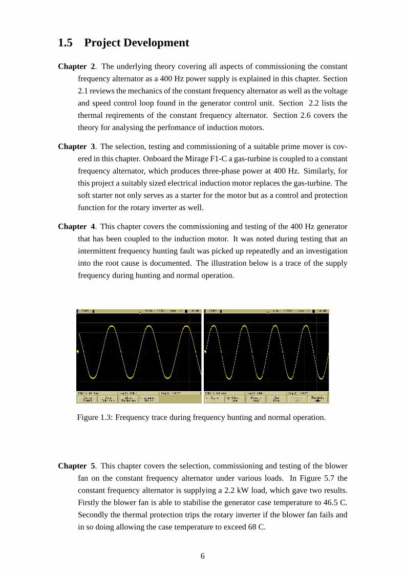
Chapter 4. This chapter covers the commissioning and testing of the 400 Hz generator
that has been coupled to the induction motor. It was noted during testing that an
intermittent frequency hunting fault was picked up repeatedly and an investigation
into the root cause is documented. The illustration below isa trace of the supply
frequency during hunting and normal operation.
Figure 1.3: Frequency trace during frequency hunting and normal operation.
Chapter 5. This chapter covers the selection, commissioning and testing of the blower
fan on the constant frequency alternator under various loads. In Figure 5.7 the
constant frequency alternator is supplying a 2.2 kW load, which gave two results.
Firstly the blower fan is able to stabilise the generator case temperature to 46.5 C.
Secondly the thermal protection trips the rotary inverter if the blower fan fails and
in so doing allowing the case temperature to exceed 68 C.
6

Figure 1.4: Constant frequency alternator’s temperature response to a 2.2 kW load withforced cooling.
Chapter 6. The chapter describes the design of the telemetering system. The system
consists of sensors, interfacing electronics, power supply and two microcontrollers.
The temperature and pressure sensors proved to interface easily, however, noise
corrupted the pressure reading which necessitated the needfor a differential summer
which solved this problem (see Section 6.2). The voltage andcurrent readings
required more thought as each reading first required rectifying and level shifting
through a precision rectifier circuit. Each sensor has been calibrated to a 0 - 5 V
scale (see Table 7.2). The telemetering system works well onvero board, however,
it would be more robust for student use if it were printed ontocircuit board (see
Figure 1.5).
Figure 1.5: The telemetering system designed for the rotaryinverter.
7

Chapter 7. The objective of this chapter was to re-use code already written by a student
who programmed a monitoring unit to measure the same four parameters, however,
what was supposed to be a straight forward exercise turned out to be a time con-
suming debugging exercise which could not be solved in the required time, for this
project. However, despite not achieving communication between boards the analog
to digital conversion as well as the decoding routines were successful.
Chapter 8. Conclusions
Chapter 9. Recommendations
8

Chapter 2
Theory Review
The underlying theory, covering all aspects of commissioning the constant frequency al-
ternator as a 400 Hz power supply, is explained in this chapter. Section 2.1 reviews the
operation of the mechanical parts of the constant frequency, as well as the voltage and
speed control loop found in the generator control unit. Section 2.2 lists the thermal re-
quirements of the constant frequency alternator. Lastly Section 2.6 covers the theory of
analysing the perfomance of induction motors.
2.1 Constant Frequency Alternator ([1],[5],[6])
The engine-driven constant frequency alternator can be thought of as a rotary converter,
in that it takes mechanical energy and converts it into electrical energy. Variable engine
speeds are passed through a constant speed drive, which turns the alternator at a set speed.
The speed at which the alternator turns determines the output frequency in these engine-
driven machines. Since the engine speed varies it is necessary for the constant speed
drive, to turn the alternator at a constant speed to keep the frequency stable at 400Hz. The
constant speed drive uses a differential gear assembly and an eddy current brake to ensure
synchronous speeds are delivered to the alternator. Synchronous speed is 8000 rpm for a
6 pole alternator to produce an output frequency of 400 Hz. Figure 1.1 shows the constant
frequency alternator, which are three-phase 200 volt line-to-line, 400 Hz machines. The
constant frequency alternator consist of: an alternator, electro-mechanical constant speed
drive and an eddy current brake cup. The electro-mechanicalconstant speed drive and
the eddy current brake cup will be referred to as the constantspeed drive and brake cup
respectively. Together these parts make it possible for thealternator to produce three-
phase 200 line-to-line voltages at 400 Hz, when driving speeds and torque fall between
2680 rpm - 8320 rpm and 77.9 N.m - 30.0 N.m [1].
9

2.1.1 Alternator
The alternator is a six pole pair synchronous machine with anoperating frequency of
400 Hz at an armature speed of 8000 rpm. Excitation is supplied through a permanent
magnet generator which consists of a fixed magnet, a half-controlled converter, exciter
and alternator winding. The magnet is stationary where the exciter winding, alternator
windings and converter rotates through the static field. Theexcited winding produces
three phase current which feeds the half-controlled converter. Controlled DC field current
is fed to the alternator rotor winding which induces a voltage across the alternator stator
winding. The stator voltage is controlled by regulating theDC field current.
Figure 2.1: Principle of operation of the alternator [1].
2.1.2 Constant speed drive
The purpose of the constant speed drive is to take rotationalengine power irrespective of
the input speed and to turn the alternator at constant speed.This is necessary to generate
400 Hz three-phase power. This consists of a differential gear assembly and a brake cup
or compensation link, as it is sometimes referred to in literature. This gear assembly is
similar to a motor vehicle’s differential transmission. Ina motor vehicle the front wheels
are allowed to rotate at different speeds to each other, so that the turning circle is reduced
when taking a corner. The differential gear action of the generator keeps the speed of the
alternator’s end constant, whereas the brake cup side changes in such a way to compensate
for the difference in speed. Equation 2.1 governs the difference speed. The equation
reads, the difference between the motor input speed and brake cup compensation speed
should be the synchronous speed of the alternator. Synchronous speed of the alternator is
8000 rpm. For motor speeds less than 4000 rpm the brake speed compensates by adding
10
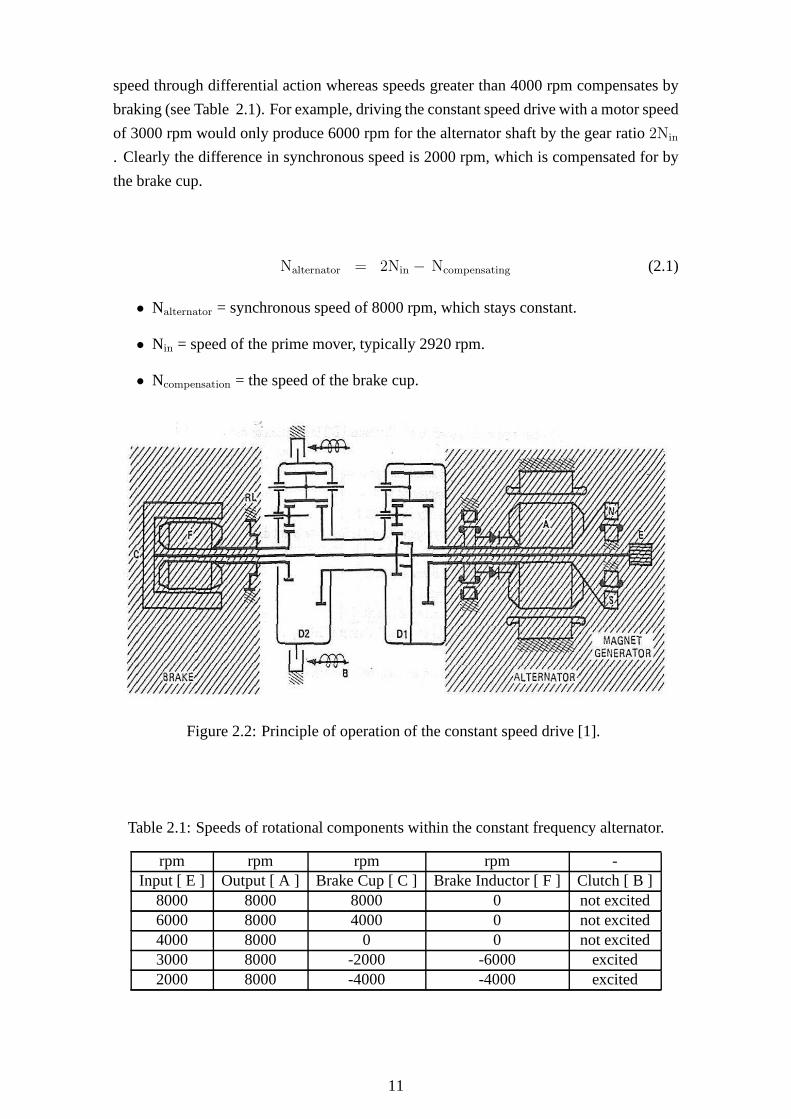
speed through differential action whereas speeds greater than 4000 rpm compensates by
braking (see Table 2.1). For example, driving the constant speed drive with a motor speed
of 3000 rpm would only produce 6000 rpm for the alternator shaft by the gear ratio2Nin
. Clearly the difference in synchronous speed is 2000 rpm, which is compensated for by
the brake cup.
Nalternator = 2Nin − Ncompensating (2.1)
• Nalternator = synchronous speed of 8000 rpm, which stays constant.
• Nin = speed of the prime mover, typically 2920 rpm.
• Ncompensation = the speed of the brake cup.
Figure 2.2: Principle of operation of the constant speed drive [1].
Table 2.1: Speeds of rotational components within the constant frequency alternator.
rpm rpm rpm rpm -Input [ E ] Output [ A ] Brake Cup [ C ] Brake Inductor [ F ] Clutch [ B ]
8000 8000 8000 0 not excited6000 8000 4000 0 not excited4000 8000 0 0 not excited3000 8000 -2000 -6000 excited2000 8000 -4000 -4000 excited
11

Calculating the ideal motor input speed [6]
The compensation power required to maintain constant speedis given by the Equation
2.2, below, which is the work of [6]. Changing the input speedand tabulating the results
from Equation 2.1 produces the results presented in Table 2.3.
Pcompensation
Pout
=Tcompensationwcompenastion
Toutwout
(2.2)
• Pcompensation- Compensation drive power
• Pout- Output power
• Tcompensation- Compensation torque
• Tout- Output torque
• wcompensation- Compensation speed
• wout- Output speed
Table 2.3 below shows that at 4000 rpm the least amount of compensation power is re-
quired from the induction motor. This infers that 4000 rpm would be the ideal prime
mover speed.
Table 2.3: Percentage of input power used to maintain synchronous speed.Nalternator[rpm] Ninput[rpm] Ncompensation[rpm] Input Power Used [%]
8000 2750 -2500 -31.258000 3000 -2000 -258000 3250 -1500 -18.258000 3500 -1000 -12.58000 3750 -500 -6.258000 4000 0 08000 4250 500 6.258000 4500 1000 12.58000 4750 1500 18.758000 5000 2000 258000 5250 2500 31.25
2.2 Thermal Characteristics [1]
The specification used for the design of the ventilation unit[1].
12
Table 2.4: The constant frequency alternator’s thermal charateristics.Power [kVA] Flow Rate [g
sec] Pressure [Pa] Period [min]
12-15 100-130 3000 indefinite10 self ventilation 20 min
2.3 The Generator Control Unit (GCU)
Seven feedback loops control the CFA output. They are contained in a shielded die-
cast rectangular box called the GCU. Stacked printed circuit board contain the control
and protection loops and are listed below. Not all the feedback loops are required for
operating the CFA in constant speed mode; those that are, arelisted below [1]:
• Voltage (196 - 200 V)
• Frequency (396 - 404 Hz)
• Over-current (> 45 A)
• Torque (sudden changes)
The most critical of these are the voltage and the frequency,which are discussed below.
2.3.1 Voltage control loop (excitation current)
Stator voltages are measured by step-down voltage transformers and compared to the
reference comparator inside the regulator. Depending on the stator voltage, the firing
angle of the rectifier’s is either increased or decreased from its set point. This regulates
the rectifiers DC voltage .The DC voltage is fed to the alternator’s rotor windings where
it becomes excitation current. This excitation current sets up the magnetic field, which
induces a voltage across the stator terminals. This is the operation of the voltage loop.
2.3.2 Frequency control loop (speed loop)
Frequency of supply is determined by the speed at which the magnetic airgap field cuts
the three pole pairs [9]. The speed of the airgap field is determined by the rotor shaft
speed. When these poles are cut at 8000 rpm, it produces 400 Hzstator voltages. The
frequency loop controls the following [1].
1. Ensuring that the alternator’s frequency falls between 396 and 404 Hz.
2. Controlling brake-cup direction and speed.
3. Engaging and disengaging differential gears.
13
2.4 Frequency Hunting [2]
The student whose research was on selecting a prime mover, preceded the work done
for this thesis, encountered a frequency hunting problem when testing the system. In an
attempt to solve the problem the student carried out the following tests.
2.4.1 Aim
The aim of this test was to compare the functioning of the working CFA from the Mirage
aircraft with the potentially faulty CFA, in order to establish whether the fault lay with the
GCU or with the CFA.
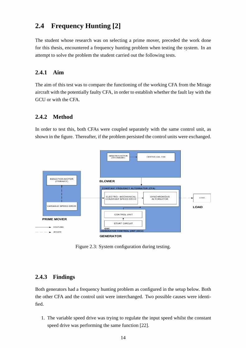
2.4.2 Method
In order to test this, both CFAs were coupled separately withthe same control unit, as
shown in the figure. Thereafter, if the problem persisted thecontrol units were exchanged.
Figure 2.3: System configuration during testing.
2.4.3 Findings
Both generators had a frequency hunting problem as configured in the setup below. Both
the other CFA and the control unit were interchanged. Two possible causes were identi-
fied.
1. The variable speed drive was trying to regulate the input speed whilst the constant
speed drive was performing the same function [22].
14

2. The frequency limiting resistor circuit were needed for constant frequency opera-
tion [22].
2.4.4 Discussion
The manner in which the variable speed drive was used was not documented by the student
whose work preceeded this project. Therefore it is assumed that the variable speed drive
operated in open loop. This open loop operation would keep the voltage and frequency
constant, which means that the induction motor would be running at 3000 rpm at full rated
torque and current [23]. If the variable speed drive was varying the input speed, then the
CSD would override any regulation in input speed. It is suggested that this might not be
the root cause.
The frequency limiting resistors are designed to brake the speed of the alternator during
rapid engine speed changes by shunting the coils across the alternator’s stator. This has the
effect of braking the alternator speed. If these resistors were faulty then the problem could
be eliminated by replacing them. When the frequency limiting resistors were removed,
however the hunting problem was still present. When the resistors were placed back,
the problem was eradicated. This reason leaves a gap in uderstanding the nature of the
hunting problem, which is addressed in the Section 4.5.
2.5 Gearbox Oil
The generator’s gearbox uses a Mobil Jet Oil 254 for lubrication. The colour of healthy
oil is brown, whereas dirty oil is black in colour. At all times the sump should be filled
with 630 ml of oil to cover moving parts. The constant frequency alternator should be
in the horizontal position while generating and re-filling with oil (see Reference [34] for
instructions on filling and re-filling of gearbox oil).
2.6 The Prime Mover
The selection of the prime mover for the constant frequency alternator formed part of an
undergraduate thesis project [2]. A 15 kW induction motor was selected; its specifications
are shown in Table 2.5 below.
15

Table 2.5: Induction motor’s rated specifications [2].Parameter Value Units
Rated Voltage 380 Vl-lRated Current 26.5 AConnection Delta/StarFrequency 50 Hz
Rated Output 15 kWSpeed at Rated Power 2940 rpmEfficiency at full load 90 %Efficiency at 3/4 load 90.2 %
Power Factor 0.90 p.uRated Torque 49 N.m
Weight 77 kg
2.6.1 The equivalent circuit model of an induction motor [9]
The per phase equivalent impedance Equation 2.3 can be used to calculate the perfor-
mance of induction motors by using the calculated parameters in Table A.3. This equation
is dependant on slips which is 1 at startup and almost zero at rated speed. In Chapter A.3
this equation is used to calculate the input impedance over the full slip range to obtain a
current profile of the induction motor.
Zin = R1 + jX1 +jXm(R2
s+ jX2)
R2s
+ j(Xm + X2)(2.3)
• R1- stator resistance
• X1- stator impedance
• Xm- magnetising impedance
• R2- rotor resistance
• X2- rotor impedance
• s - slip
The stator current Equation2.4 below uses the phase-to-neutral voltageVph at different
input impedancesZin to calculate the startup currentIs (see Equation 2.4).
Is =Vph
Zin
(2.4)
16

• Is - stator current.
• Vph - phase to neutral voltage.
• Zin - input impedance.
Equation 2.5 determines the available torque which the induction motor can be loaded
with at startup. The equation uses the thevenin equivalent voltageVth and impedanceRth
andXth as the stator parameters in the calculation, (see Reference[8]). This equation can
be used for determining a torque profile for the motor.
Tem =1
wsync
×(Vth)
2
(Rth + R2
s) + (Xth + X2)2
(2.5)
The motor equationN = 120fp
shows that a two pole (p) induction machine on a 50 Hz (f)
supply has a maximum speed 3000 rpm.
17

Chapter 3
Commissioning the Siemens 15 kW
Induction Motor as the Prime Mover
for the Constant Frequency Alternator
The selection, testing and commissioning of a substitute prime mover is covered in this
chapter. Onboard the Mirage F1-C, a gas-turbine is coupled to a constant frequency alter-
nator, which produces the mechanical power to generate three-phase power at 400 Hz. In
the method used in this dissertation, the induction motor replaces the gas-turbine.
3.1 Prime Mover Selection
3.1.1 Constant frequency alternator’s specifications
The driving shaft requirements show that the constant frequency alternator can operate in
two power modes i.e at high and low rotational speeds. Table 3.1 lists the requirements
for driving the constant frequency alternator in both modes.
It is the function of the constant speed drive to deliver constant rotational speed at 8000
rpm to the alternator rotor irrespective of the input speed.For the purpose of maintaining
constant rotor speed the constant speed drive includes two differential gears and an elec-
tro mechanical brake all controlled by the frequency regulation system of the regulator.
Therefore it is not necessary for both the motor and the constant speed drive speeds to be
regulated.
Table 3.1: The constant frequency alternator’s power rating at different speeds.Power Rating [kVA] PF Rotational Speeds [rpm] Torque [N.m]
15 0.75 5600 - 8320 77.912 0.75 2680 - 5600 30.4
18

3.1.2 Direct current motors versus induction motors
Since speed control is not required on the motor side an ordinary DC or an AC induction
motor can be used. Induction motors are more viable than DC motors, because the latter
have brushes that require maintenance [9]. As a result, an induction motor was chosen.
3.1.3 Induction motors
The ideal motor would be a 4000 rpm at 30.4 N.m machine, which is explained in Sec-
tion 2.1.2. However this cannot be achieved in an induction machine due to the speed
limitation on a 50 Hz supply (see Section 2.6). The availablemotor sizes in this range
are 11, 15 and 18 kW. The 11 kW motor has insufficient torque, whereas an 18 kW has a
surplus at a higher cost, for this reason a 15 kW induction motor was chosen. Table 3.1
lists the motor’s requirements.
Table 3.2: Characteristics of the prime mover.Parameter Value Unit
Rated Voltage 380 Vl-lRated Current 26.5 ARated Output 15 kWRated Torque 49 N.m
Speed at rated output2940 rpmFrequency 50 HzConnection O/Y
3.2 Pre-Commissioning Work
3.2.1 Induction motor testing
A no load and locked rotor test was performed on the motor to calculate the equivalent
circuit, which enables the following current profile to be predicted. These test results can
be found in Appendix A. The following graph was created usingthe formulaIstator =Vph
Zin
where Vphand Zinare phase voltage and input impedance respectively. The phase voltage
is 220 V and 380 V in a star and delta connected network respectively. Input impedance
is calculated using Equation A.13 over the slip interval, and plotted for the star and delta
configurations as shown below. The graph in Figure 3.1 shows the motor’s phase-current
profile under the star and delta configurations versus slip. The green curve represents
the current profile of the star configuration, whereas the yellow curve represents that of a
delta configuration. The result is consistent with the literature, which predicts a 5-8 times
larger starting current [8]. It was found that the startup current causes nuisance-tripping
19
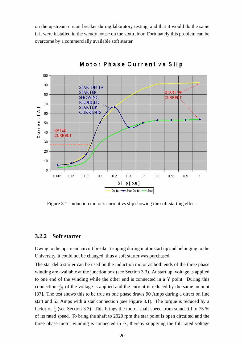
on the upstream circuit breaker during laboratory testing,and that it would do the same
if it were installed in the wendy house on the sixth floor. Fortunately this problem can be
overcome by a commercially available soft starter.
Figure 3.1: Induction motor’s current vs slip showing the soft starting effect.
3.2.2 Soft starter
Owing to the upstream circuit breaker tripping during motorstart up and belonging to the
University, it could not be changed, thus a soft starter was purchased.
The star delta starter can be used on the induction motor as both ends of the three phase
winding are available at the junction box (see Section 3.3).At start up, voltage is applied
to one end of the winding while the other end is connected in a Ypoint. During this
connection 1√3
of the voltage is applied and the current is reduced by the same amount
[37]. The test shows this to be true as one phase draws 90 Amps during a direct on line
start and 53 Amps with a star connection (see Figure 3.1). Thetorque is reduced by a
factor of 13
(see Section 3.3). This brings the motor shaft speed from standstill to 75 %
of its rated speed. To bring the shaft to 2920 rpm the star point is open circuited and the
three phase motor winding is connected in∆, thereby supplying the full rated voltage
20

and current to the motor and allowing it to reach full speed. The configuration for the
starter shows the following switchgear viz, thermal overload relay, timer, delta and star
contactors. The time the soft starter takes to make the transition between star and delta is
set to 12 seconds. The thermal overload is set to trip once thecurrent drawn exceeds 1.1
times rated current (29.3 A).
Figure 3.2: Soft starter’s schematic.
3.2.3 Motor connections
The terminal connections are colour coded as illustrated inFigure 3.3. The connections
W2, U2, V2 are wired from the overload relay whereas U1, V1, W1are connected to the
star and delta contactors. Not shown is the earth connectionto the motor case which must
be secured to ensure earth fault protection.
21
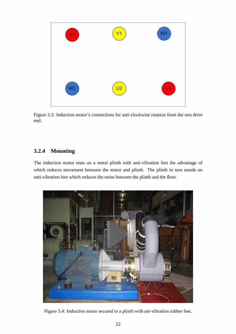
Figure 3.3: Induction motor’s connections for anti-clockwise rotation from the non driveend.
3.2.4 Mounting
The induction motor rests on a metal plinth with anti-vibration feet the advantage of
which reduces movement between the motor and plinth. The plinth in turn stands on
anti-vibration feet which reduces the noise between the plinth and the floor.
Figure 3.4: Induction motor secured to a plinth with ant-vibration rubber feet.
22

3.3 The Load Torque
It was assumed that the load would impose a torque of 30.4 N.m on the motor as soon as
the load circuit breaker is closed on the generator side. Theassumption was based on Ta-
ble 3.1. During the star connection the motor’s torque is less than 30.4 N.m, which would
result in a stall if the coupled generator were started with aload attached. A stall occurs
when there is a negative difference between the motor’s and load’s torque. Figure 3.5 was
calculated based on Equation 2.5 which clearly shows the motor’s torque versus slip. The
motor did stall while the generator with load was started during the reduced torque state
as shown by the fuchsia curve outside the red vertical lines in Figure 3.5. To solve this,
the generator should not start under the star contactor but that it should be synchronised
with the delta contactor. This is covered in Subsection 4.3.
Figure 3.5: Induction motor’s torque vs slip showing the soft starting effect.
23

3.4 Starting and Stopping the Prime Mover
The induction motor is started and stopped via the push button on the front panel of the
soft starter, provided that the mains supply is switched on.The generator and blower fan
will be re-wired to start from the soft starter (see Sections4.3 and 5.4 respectively).
3.5 Motor Efficiency
Using the name plate table parameters we can calculate the input power to the motor to
be :
Pin = 3 × V × I × cosΘ
Pin = 3 × 400 ××15.40.9
Pin = 16632W
Using the rated torque and shaft speed we can calculate that the induction motor is rated
to deliver :
Pout = Trated × ωrated
Pout = 49N.m×314rad
secPout = 15386W
The rated efficiency of the Siemens induction motor isPoutPin
= 92.5 %.
3.6 Summary
In conclusion, the chapter provided the following useful information, viz:
• Nuisance tripping was resolved by the use of the soft starter.
• The soft starter serves as a central point of control for the motor, generator and
blower fan.
• The generator cannot be started when the motor is operating in the reduced torque
mode, owing to the fact that there is insufficient torque.
• Motor efficiency is calculated to be 92.5%.
24

Chapter 4
Commissioning the 400 Hz Generator
This chapter covers the design of the generator control unit’s starter circuit, commission-
ing and testing of the 400 Hz generator, the investigation into the intermittent frequency
fault, the proposals for determining root cause for frequency failure and the investigation
into the discolouration of the gearbox oil. The constant frequency alternator and generator
control unit will hereafter be referred to as the CFA and GCU respectively.
4.1 Design of the Generator Control Unit’s Starting Cir-
cuit (GCUSC)
The GCU is powered from the permanent magnet generator inside the CFA as soon as the
input speed reaches 2600 rpm via relay K1. Relay K1 closes thethree phase AC windings
of the permanent magnet generator onto the power regulator circuit inside the GCU. The
circuit needed to close K1 should source 28 Vdc at a minimum of200 mA. Onboard
the aircraft this power would come from the battery banks, which would be used for the
essential auxiliaries required to start the aircraft. The GCUSC receives 220 VAC via the
red phase and neutral from the motor’s soft starter. See Section 4.3 for synchronising the
GCUSC to the soft starter.
4.1.1 Calculating componet sizes for the GCUSC
Capacitor C2 couples 28 V via a 3 pin molex connector to the GCU. Taking into consid-
eration a 4 V drop across the LM317 regulator and bridge rectifier (B1), the secondary
transformer voltage should compensate for the voltage dropwhich shall be 32 Vrms. A
24 V transformer can be used if small currents are being drawn. This is because capacitor
C1 charges to the peak of the rectified output across B1, (√
2 x 23V). This was measured
and this is why a 24 V secondary transfomer was chosen. For protection a 20 mA fuse is
selected according to the tranfomer equationV2A2
V1where A2 is 200 mA.
25

Figure 4.1: Schematic for the generator control unit’s starting circuit.
The component values for the GCUSC is listed in Table 4.1.
Table 4.1: Component values of the GCUSC.Component Value Component Value
Vout 28V LM317 AdjustableIout 200 ma C1 1000uFIin 23 mA C2 470uF
Transformer 24 VA Fuse 20 mA
The GCUSC supplies 200 mA at 28 Vdc.
4.2 Alternator Load and Power Factor Test Results
Figure 4.2 shows the test setup for the system. The setup includes an induction motor
mechanically coupled to the alternator via a solid coupling, while the blower fan is sup-
plying forced air through a shroud over the alternator. The blower fan is not shown in the
figure.
Due to the laboratory equipment limitations only one Chauvin Arnoux power meter and
two Fluke multimeters were available to be used for measurements and metering. The
Chauvin Arnoux power meter was connected with voltage probes across the motor termi-
nals, while current probes were clamped over the individualphases of the supply power
cable to the motor. The load is balanced therefore one phase of the load is measured and
the total power is calculated by multiplying by the single phase result by 3. One Fluke
meter measured voltage across the red and blue phase, while the other measured current
in the red phase.
The alternator was tested with resistor banks. Three banks were used where each bank
consisted of 4 resistors. Each resistor had impedance of Z =60∠0.053 . The inductances
of these resistors are considerably low and the power factoris close to 0.99 even in the
worst case where all resistors are connected in series.
26
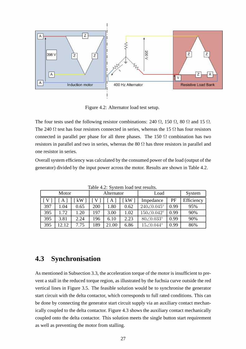
Figure 4.2: Alternator load test setup.
The four tests used the following resistor combinations: 240 Ω, 150Ω, 80 Ω and 15Ω.
The 240Ω test has four resistors connected in series, whereas the 15Ω has four resistors
connected in parallel per phase for all three phases. The 150Ω combination has two
resistors in parallel and two in series, whereas the 80Ω has three resistors in parallel and
one resistor in series.
Overall system efficiency was calculated by the consumed power of the load (output of the
generator) divided by the input power across the motor. Results are shown in Table 4.2.
Table 4.2: System load test results.Motor Alternator Load System
[ V ] [ A ] [ kW ] [ V ] [ A ] [ kW ] Impedance PF Efficiency397 1.04 0.65 200 1.80 0.62 240∠0.045 0.99 95%395 1.72 1.20 197 3.00 1.02 150∠0.042 0.99 90%395 3.81 2.24 196 6.10 2.23 80∠0.033 0.99 90%395 12.12 7.75 189 21.00 6.86 15∠0.044 0.99 86%
4.3 Synchronisation
As mentioned in Subsection 3.3, the acceleration torque of the motor is insufficient to pre-
vent a stall in the reduced torque region, as illustrated by the fuchsia curve outside the red
vertical lines in Figure 3.5. The feasible solution would beto synchronise the generator
start circuit with the delta contactor, which corresponds to full rated conditions. This can
be done by connecting the generator start circuit supply viaan auxiliary contact mechan-
ically coupled to the delta contactor. Figure 4.3 shows the auxiliary contact mechanically
coupled onto the delta contactor. This solution meets the single button start requirement
as well as preventing the motor from stalling.
27

Figure 4.3: The soft starter with synchronising auxiliary contact.
4.4 Pre-Commissioning Work
4.4.1 Testing the CFA and GCU according to the commissioningin-
structions provided by the generator manual
The first evaluation tests the excitation current loops of the GCU according to the CFA’s
technical manual. It can be deduced from the results in Table4.3 that the control circuit
is operating properly for low speeds1.
Table 4.3: Comparing the measured excitation current against the technical manual’s.Clutch (Coil E)
Terminals Documented Amps Measured AmpsE-N 0.5 - 0.8 0.66 - 0.7
Clutch (Coil F)Terminals Document Amps Measured Amps
F-N 0.15 - 0.25 0.16 - 0.22
Brake (Coil B)Terminals Document Amps Measured Amps
L-M 0.8 - 1.2 0.07 - 1.2
The second test performed was to verify whether the electrical insulation of the generator
is good. A weak spot in the insulation would cause a short on the winding, which can
1For speeds less than 4000 rpm the method of speed control is governed by the brake and clutch coils.These work together in order to engage a speed doubling gear.
28

be picked up by measuring the resistance. The results from Table 4.4 suggest that the
insulation strength of the generator is satisfactory. Fromthe test results obtained, it can
be concluded that the generator is in a condition to be used.
Table 4.4: Winding resistance values.alternator’s phase windings
Terminals DocumentedΩ MeasuredΩA-N 0.109 - 0.134 0.122B-N 0.109 - 0.134 0.119C-N 0.109 - 0.134 0.121alternator inductor (excitation control)
Terminals DocumentedΩ MeasuredΩR-P 23.6 - 28.6 28.4
brake inductorTerminals DocumentedΩ MeasuredΩ
L-M 6 - 7.5 7.1magetic clutch coils
Terminals DocumentedΩ MeasuredΩN-E 147 - 179 172N-F 27 - 33 31
pulse generator windingsTerminals DocumentedΩ MeasuredΩ
S-V 6.3 - 7.7 6.98V-N 1.53 - 1.87 2.75S-N 7.83 - 9.57 8.68
permanent magnet generator phase coilsTerminals DocumentedΩ MeasuredΩ
T-G 0.75 - 1 DNMG-H 0.75 - 1 DNMH-T 0.75 - 1 DNM
frequency limiting resistorsTerminals DocumentedΩ MeasuredΩ
U-J 11 - 14.5 12.75J-K 11 - 14.5 12.75K-U 11 - 14.5 12.75
4.4.2 Wiring harness
As the existing wiring harness had perished and required repairing, a new harness was
made connecting the CFA to the GCU and the GCUSC. The harness uses amphenol con-
nectors. The harness is 3 m in length and was tested for continuity (see Section B).
29

Figure 4.4: Constant frequency alternator’s wiring harness.
4.5 Frequency Hunting
Frequency hunting is the intermittent problem of the alternator trying to keep its output
at 400 Hz but instead oscillating between 328 and 336 Hz. The voltage during frequency
hunting is 200 volts line-to-line [2].
The first signs of frequency hunting appeared while a previous student was working on
the CFA. In an attempt to find the cause of the problem the student checked the motor,
motor starter and wiring harness connections first before obtaining a replacement CFA and
GCU off the same Mirage from Leon Heinkelin. Leon is an engineer at the University of
Stellenbosch who has experience with these aircraft power supplies, and he was asked to
investigate.
The first investigation tried to establish whether the CFA orGCU was faulty. Leon’s GCU
was thus used to control the CFA. However, frequency huntingstill occurred. Thereafter
the GCU was used to control Leon’s CFA where frequency hunting failed to occur. The
first investigation thus concluded that the problem lay withthe CFA.
The second investigation sought to establish which component in the CFA was faulty. The
frequency limiting resistors were disabled, as they were thought to be faulty. These resis-
tors shunt the alternator when the engine speed of the aircraft accelerates or decelerates
faster than 1000 rpm per second. Shunting across all three phases weakens the magnetic
field so that the rotor slows down and hence the frequency dips. When these resistors
were re-enabled, it was documented that the CFA no longer suffered from the spurious
frequency hunting problem [2].
During commissioning of the CFA however, the spurious frequency hunting problem re-
appeared and when the frequency limiting resistors were disabled and re-enabled the prob-
30
lem remained. Leon was contacted in October 2006 in which time the wiring harness,
coil resistances, excitation currents, frequency limiting resistors, frequency control cir-
cuit, fuses and brushes were checked and all were found to be within specification (see
Section B).
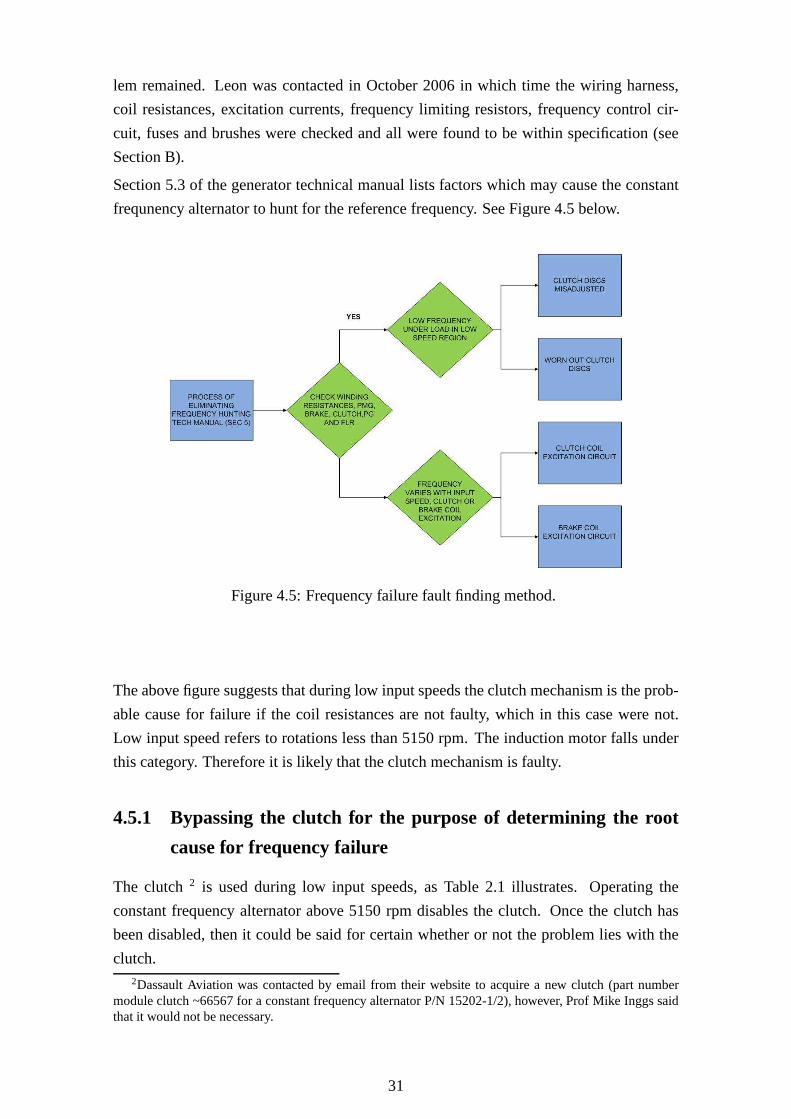
Section 5.3 of the generator technical manual lists factorswhich may cause the constant
frequnency alternator to hunt for the reference frequency.See Figure 4.5 below.
Figure 4.5: Frequency failure fault finding method.
The above figure suggests that during low input speeds the clutch mechanism is the prob-
able cause for failure if the coil resistances are not faulty, which in this case were not.
Low input speed refers to rotations less than 5150 rpm. The induction motor falls under
this category. Therefore it is likely that the clutch mechanism is faulty.
4.5.1 Bypassing the clutch for the purpose of determining the root
cause for frequency failure
The clutch2 is used during low input speeds, as Table 2.1 illustrates. Operating the
constant frequency alternator above 5150 rpm disables the clutch. Once the clutch has
been disabled, then it could be said for certain whether or not the problem lies with the
clutch.2Dassault Aviation was contacted by email from their websiteto acquire a new clutch (part number
module clutch ~66567 for a constant frequency alternator P/N 15202-1/2), however, Prof Mike Inggs saidthat it would not be necessary.
31

One method of operating the system as is above 5150 rpm would be to over-excite the
induction motor by using a variable speed drive. This could be done only for testing
the output frequency of the generator with no load attached,due to the drop in torque
experienced in this mode it would be unwise to couple a load tothe generator [8]. Care
must be exercised not to operate the induction motor for too long a time as the bearings
are not rated for speeds higher than 3000 rpm [25], [27]. If bypassing the clutch solves
the problem then it is suggested that Dassault Avionics should be contacted regarding a
replacement clutch.
4.5.2 Changing the induction motor with a dc motor
In conversation with Professor Mike Case from the University of Johannesburg, the stu-
dent’s attention was brought to another theory behind the frequency hunting problem. The
theory behind the conversation is that as the CSD regulates the alternator’s speed, the in-
duction motor experiences a change in load. The problem withthis is that as the induction
motor’s load changes, so does it’s speed. The change in motorspeed fights against the
CSD’s action, which is trying to keep the alternator at 8000 rpm. This fighting between
the CSD and motor could be a possible cause for the problem of frequency hunting. The
solution would be to use a gearbox coupled to either a synchronous reluctance or DC
motor which does not share the same load-speed relationshipas do induction motors. It
would be satisfying to test the merits behind both theories,perphaps as a further research
topic.
4.6 Discolouration of the Gearbox Oil
This section lists the possible factors which could result in the gearbox oil discolouring.
Associate Professor Andy Yates from the deparment of mechanical engineering at the
University of Cape Town was consulted to identify the possible causes for the discoloura-
tion.
4.6.1 Incorrect oil viscosity
Low viscose oil will barely cover metal surfaces inside a gearbox, thus leaving exposed
areas, which can result in metal to metal friction. Such friction would cause the accumu-
lation of metal particles suspended in the oil sump.
Oil with a high viscosity would sufficiently cover metal surfaces but will result in heat
losses, as the CFA tries overcome the drag imposed on it by theoil. This excessive heat
generated by the gearbox would cause premature oil degradation.
Mobil Jet Oil II is the recommended oil to be used in the CFA’s gearbox [33].
32

Table 4.5: Mobil Jet Oil II characteristics.Properties Values
Viscosity at 100C 27.6 cSTFlash point 270CFire point 285C
4.6.2 Combustion of oil
Oil in a car’s engine that makes its way past the piston rings would mix with the combus-
tion mixture, resulting in oil burning and hence discolouration. The end result is black oil
in the gearbox sump.
4.6.3 Incorrect oil level
The required volume of oil is 800ml and this can be checked when oil no longer flows
passed the refill valve. Too much oil will result in the unit malfunctioning, whereas too
little oil would cause metal to metal friction [34].
4.6.4 Findings
During the project the gearbox oil was replaced twice with anamount of 630 ml. A
syringe was used to refill the gearbox with oil. The reason forusing this amount and not
800 ml is because at this point no more oil could be forced passed the refill valve, which
is when the manual suggests that the gearbox is filled. My assumption at the time was
that during emptying, not all the oil could be removed. If my assumption was right, then
the gearbox had a sufficient amount of oil covering the metal surfaces and that another
factor resulted in the oil discolouring. If my assumption was wrong, then the gearbox
was running low on oil and chances are that there was metal to metal friction inside the
gearbox which more than likely resulted in the premature degradation of the oil.
4.6.5 Conclusions
Table 4.5 shows that the oil grade used is within the suggested viscosity range, which
can rule out viscosity as the cause of the discolouration of oil. Combustion, too, can be
ruled out due to the fact that it is gearbox oil that is being discoloured and not oil in the
engine. I suspect that my original assumption might have been wrong, which resulted
in the operation of the CFA with a low amount of gearbox oil to protect the metal parts
inside the CFA. This could have been caused by the fact that I did not apply enough force
onto the syringe to force oil passed the refill valve.
33

Figure 4.6: Tools used to re-fill the gearbox sump
4.6.6 Recommendation
The syringe and nozzle used were not the proper tools for the job of re-filling a pressurised
sump. This requires tools that exert a big enough force to pass oil through a valve and
into a sump. I recommend that a pressurised oil feeder be usedfor the re-filling of oil in
future.
4.7 Transients
The effects of transients on the 400 Hz rotary inverter couldnot be investigated, owing to
the frequency hunting problem.
4.8 Summary
In conclusion, the chapter provided the following useful information, viz:
• The GCUSC was designed, built and tested.
• Pre-commissioning work concludes that the CFA, GCU and new wiring harness is
functional.
• It is propable that discoloration of the gearbox oil was caused by running the CFA
with too little oil in the sump.
• The 400 Hz Generator is not in a state to be commissioned untilthe frequency
hunting problem is solved.
34

Chapter 5
Blower Fan Design
Onboard the aircraft the CFA is supplied with forced air bledfrom the compressor of the
jet engine turbine for it to operate properly. The operatingtemperature of the constant
frequency generator shall not fall below -50 C and rise above80 C while the generator
control unit shall not exceed -50 C and rise above 85 C [35]. Operating the constant
frequency generator continuously requires forced ventilation. Generating at 10 kVA or
less the constant frequency generator is allowed to self-ventilate for a period not exceeding
20 minutes [35]. The recommended forced ventilation flow rate should be 130gs
/ 11 m3
s
over the eddy current brake and 100g
sover the alternator at a pressure of 3 kPa. These are
recommended conditions for the constant frequency generator to operate properly1. The
rest of the chapter covers the selection and testing of the blower fan unit.
5.1 Actual CFA Heating
Four tests were conducted in the Goodlet laboratory in orderto establish the actual heat-
ing of the CFA, without forced air cooling. A no load, 2.5 kW, 5kW and a 7.5 kW test
was carried out under the same temperature conditions and using the same thermocou-
ple temperature sensor. Temperature readings were recorded at the same intervals for 4
minutes. The no load test clearly shows that the CFA generates heat by the friction of its
rotating parts. The remaining tests shows that forced cooling is necessary as each trend
line approaches the maximum temperature at different ratesin Figure 5.1.
5.2 Blower Fan Selection Process
Alstom Manufacturer’s use the selection chart for choosinga blower fan for a specific
application (see Figure 5.2). There are four factors that are used in the selection process.
1The generator control unit is built on an aluminium heatsink.
35

Figure 5.1: Actual heating of the constant frequency alternator.
These four factors are required flowrate, the required pressure, the altitude and the tem-
perature of the environment. The required flowrate and pressure are read off the chart
in Figure 5.2, which is made for standard temperature and atmospheric conditions. This
implies that derating pressure and flowrate according to thecorrection factors found in
the Alstom centrifugal fan selection guide (see Reference [21]). These correction factors
can be neglected due to the fact that the blower fan is situated in Cape Town2 and the
temperature deviation is small. The blower is selected by matching the flowrate (11m3
s)
at the pressure required (3 kPa) by using the chart. The chartselects the 4P-1 blower fan
with the following characteristics (see Table 5.2). The table compares Alstom’s model to
that of Veritech’s. Veritech was the manufacturer selectedto design the blower fan.
Table 5.1: Comparison between an Alstom and a Veritech blower fan.Characteristic Alstom Veritech
Blade Type Radial RadialBlade Diameter 1,05m 1,05
Speed 1500 rpm 3000Motor 4 kW 2.2 kWPoles 4 2
2Cape Town is at sea level thus derating can be neglected.
36

Figure 5.2: The blower fan selection chart by Alstom.
5.3 Cooling Ducts and Shroud
Provision is made for air to pass over the electrical windings of the CFA via two inlet
vents and exit via two exhaust vents. Cooling is needed so that the winding insulation
does not perish, which would result in a short circuit between windings.
Previous work done by a student incorrectly documented the position of the two inlet and
two exhaust vents. Based on the student’s work dimensions for inlet ducts were designed
and built for the exhaust vents which could not be interchanged. These ducts were then
installed over the CFA exhaust vents instead of the inlet vents. Operating the blower fan
with air passing into the exhaust vents had a negligible cooling effect on the generator [2].
This is why a shroud was designed and built, which provided sufficient cooling. The
rates of cooling and the shroud dimensions are summarised inSections 5.6.3 and C.2
respectively.
37

Figure 5.3: Cooling ducts also showing the apparatus used tomeasure flowrate.
Figure 5.4: The cooling shroud.
5.4 Blower Fan Starter
The blower’s motor uses a push button operated contactor forstarting, which uses 220
VAC to make and break electrical contact. However, this doesnot meet the user require-
38
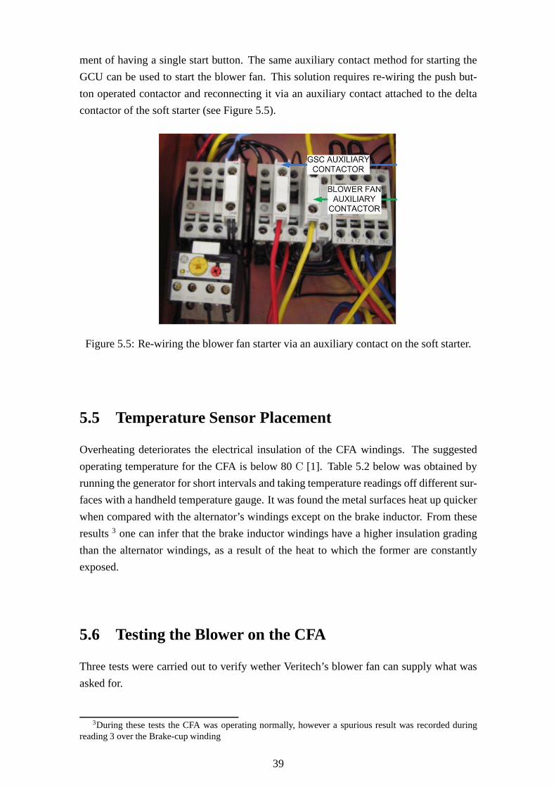
ment of having a single start button. The same auxiliary contact method for starting the
GCU can be used to start the blower fan. This solution requires re-wiring the push but-
ton operated contactor and reconnecting it via an auxiliarycontact attached to the delta
contactor of the soft starter (see Figure 5.5).
Figure 5.5: Re-wiring the blower fan starter via an auxiliary contact on the soft starter.
5.5 Temperature Sensor Placement
Overheating deteriorates the electrical insulation of theCFA windings. The suggested
operating temperature for the CFA is below 80C [1]. Table 5.2 below was obtained by
running the generator for short intervals and taking temperature readings off different sur-
faces with a handheld temperature gauge. It was found the metal surfaces heat up quicker
when compared with the alternator’s windings except on the brake inductor. From these
results3 one can infer that the brake inductor windings have a higher insulation grading
than the alternator windings, as a result of the heat to whichthe former are constantly
exposed.
5.6 Testing the Blower on the CFA
Three tests were carried out to verify wether Veritech’s blower fan can supply what was
asked for.
3During these tests the CFA was operating normally, however aspurious result was recorded duringreading 3 over the Brake-cup winding
39

Table 5.2: CFA hotspot readings on load.Test Position Placement Region Reading 1 Reading 2 Reading 3
1 Heatsink Top 47.0 59.4 69.02 Heatsink Oil Plug 44.6 58.0 71.63 Heatsink J1a Connector 40.0 49.0 60.24 Brake-cup winding 41.0 49.0 54.25 Brake inductor windings 55.0 64 *6 Alternator windings 37.0 43.0 51.0
Figure 5.6: The 400 Hz rotary inverter.
40

5.6.1 Flowrate test
At the time this test was carried out the old cooling ducts were used and were incorrectly
placed due to the reason given in Section 5.3. A cardboard cube was made to fit around
the “exhaust vent” while the cooling ducts were positioned over inlet vents and forced air
was allowed to pass through (see Figure 5.3). The exiting flowrate was measured through
a window of 40 mm x 30 mm in size at a distance of 750 mm (see Figure C.1). An
anemometer was borrowed from the department of mechanical engineering and used to
measure the airspeed. Flowrate is calculated using the Equation Q = A.v. The flowrate
measured is shown to be 94m3
swhich is 8 times the flowrate required.
Table 5.3: Blower fan flowrate measurement.Result Airspeed [ v ] Area [ A ] Flowrate [ Q ]
1 40ms−1 2.35m2 94m3
s
5.6.2 Pressure test
A pressure transducer placed inside the cooling shroud perpendicularly to the airflow pro-
duces a static reading as opposed to placing it inline to the airflow [36]. The fullscale
reading on the pressure transducer is 17 mV at 7 kPa, however,a noisy signal was mea-
sured. Due to the fact that the noise on the signal was greaterthan the fullscale transducer
reading, this test proved to be inconclusive. Amplifying the transducer reading solved this
problem (see Section 6.2).
5.6.3 Temperature test
The figures below shows the temperature response of the generator to a 2.2 and a 4.8 kW
load.
41

Figure 5.7: CFA’s temperature response to a 2.2 kW load with forced cooling.
Figure 5.8: CFA’s temperature response to a 4.8 kW load with forced cooling..
Testing the blower fan at the required 2.2 kW load
A 2.2 kW load was coupled to the CFA, the power required by the Blue Parrot radar’s
distribution board, which yielded the following useful results (see Figure 5.7) :
1. The stabilising temperature lies between 45.5C and 46.5C when supplying its
rated load under forced cooling.
2. Thermal protection operates between 65C and 68C.
3. The time it takes to stabilise the CFA’s temperature is 11 minutes.
42

Testing the CFA at 4.8 kW
The test provided the following results (see Figure 5.8) :
1. The stabilising temperature lies between 54C and 54.5C.
2. The time it took to stabilise the CFA’s temperature is 6.5 minutes.
5.7 Summary
In summary this chapter provided the following information:
• The blower fan delivers more than the required flowrate.
• The previous student recorded the incorrect airflow direction resulting in the design
of the wrong ducts, which caused the CFA to overheat. The overheating problem
was corrected by the design of the cooling shroud, which not only directs airflow
over the electrical windings but over the heatsink as well.
• The stabilising temperature is between 45.5C and 46.5C when supplying its rated
load under forced cooling.
• The time it takes to stabilise the CFA’s temperature is 11 minutes for it’s rated load.
• Thermal protection operates between 65C and 68C.
43

Chapter 6
Telemetering System Design
The Oxford dictionary defines a telemetering system as an apparatus for recording the
readings of an instrument and transmitting them by radio. For the purposes of this project
the 400 Hz rotary inverter is the instrument, the apparatus for recording are two microcon-
trollers and radio frequency transmission is achieved through a transmitter and receiver.
The parameters measured from the 400 Hz rotary inverter are:(1) single phase line-to-line
voltage across red-and-blue phase, (2) current in the red phase, (3) ventilation pressure
inside the cooling shroud, and (4) rotary inverter’s case temperature.
The two microcontrollers used are based on the HC908Jk1 development board designed
by Sam Ginsberg. Each development board uses a 14.7456 MHz clock, 12 ADC channels
with 8 bit resolution, 1.5 Mb of flash memory, 4 push buttons and an LCD. Four ADC
channels [1:3, 9] would digitise the four parameters mentioned in the above paragraph and
send the signal over the serial pin PTB0. The receiver would actively wait for the serial
data on PTB0 before displaying it over the LCD. The radio frequency (RF) transmitter
connects to PTB0 on the transmitter and sensor board where the RF receiver connects
to PTB0 on the receiver and display boards. Both RF modules operate on the amateur
band 433 MHz and uses 17 cm whip antennae. Unfortunately the telemetering system
communicates by a fixed link, shown in the picture by a red wire, instead of the RF
transmitter and receiver.
Now each reading will be explained.
44

Figure 6.1: The telemetering system designed for the rotaryinverter.
45

6.1 Temperature Measured from the Rotary Inverters Case
The LM35DZ measures the rotary inverters case temperature which should not exceed 80
C. The temperature sensor outputs 10 mV for every degree risein temperature over a 0 -
150 C range. The LM35DZ temperature sensor is used for measuring the case temperature
only.
Thermal protection comes in the form of a bi-metal switch glued with Pratley adhesive to
the case. The bi-metal switch is closed under normal operating temperatures and open cir-
cuits between 65 - 70 C. The bi-metal sensor is placed in series with the main switchgear
panels stop switch (see Figure A.3).
6.1.1 LM35DZ and bi-metal sensor placement
Table 5.2 shows hot spot readings taken from the surface of the rotary inverter, alternator
and brake windings. The LM35DZ was placed on the warmest flat surface for measuring.
The bi-metal is placed on the same surface as the LM35DZ temperature sensor.
Figure 6.2: LM35DZ and Bi-metal temperature sensor and switch placement.
46
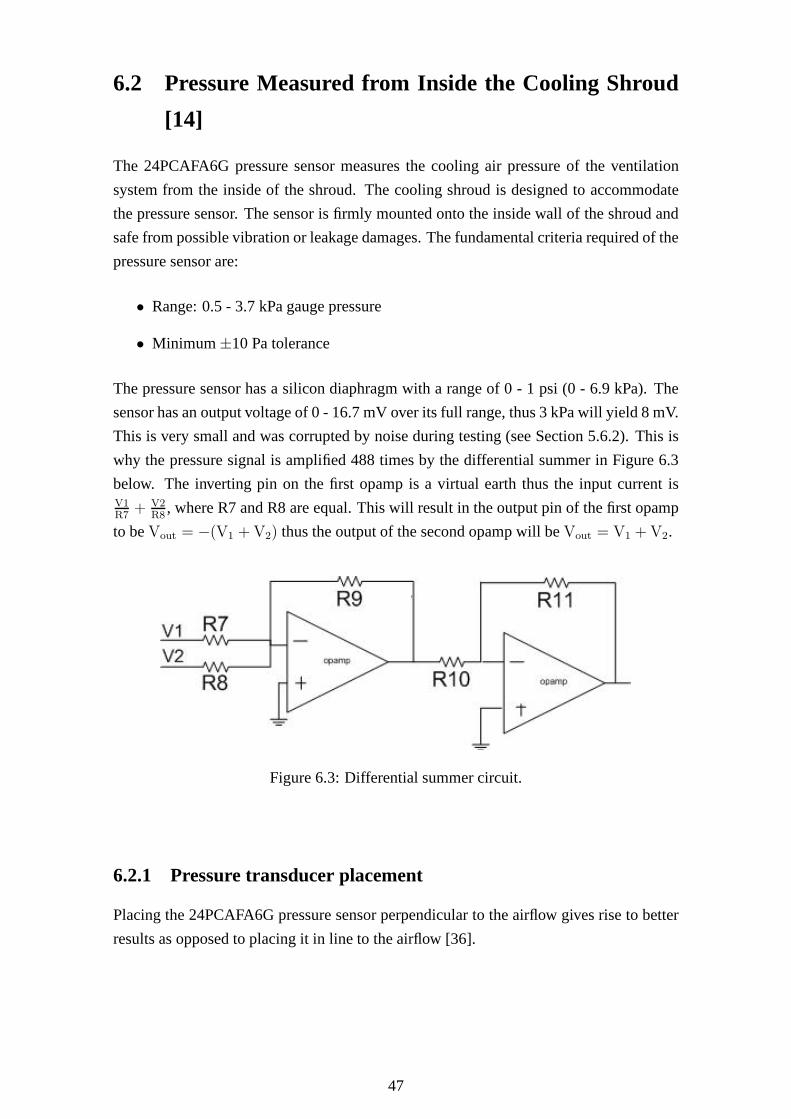
6.2 Pressure Measured from Inside the Cooling Shroud
[14]
The 24PCAFA6G pressure sensor measures the cooling air pressure of the ventilation
system from the inside of the shroud. The cooling shroud is designed to accommodate
the pressure sensor. The sensor is firmly mounted onto the inside wall of the shroud and
safe from possible vibration or leakage damages. The fundamental criteria required of the
pressure sensor are:
• Range: 0.5 - 3.7 kPa gauge pressure
• Minimum±10 Pa tolerance
The pressure sensor has a silicon diaphragm with a range of 0 -1 psi (0 - 6.9 kPa). The
sensor has an output voltage of 0 - 16.7 mV over its full range,thus 3 kPa will yield 8 mV.
This is very small and was corrupted by noise during testing (see Section 5.6.2). This is
why the pressure signal is amplified 488 times by the differential summer in Figure 6.3
below. The inverting pin on the first opamp is a virtual earth thus the input current isV1R7
+ V2R8
, where R7 and R8 are equal. This will result in the output pin of the first opamp
to beVout = −(V1 + V2) thus the output of the second opamp will beVout = V1 + V2.
Figure 6.3: Differential summer circuit.
6.2.1 Pressure transducer placement
Placing the 24PCAFA6G pressure sensor perpendicular to theairflow gives rise to better
results as opposed to placing it in line to the airflow [36].
47

Figure 6.4: 24PCAFA6G pressure sensor placement.
6.3 Current Measured in the Red Phase
The current LEM is located on the same board as the voltage sensor. To measure a typical
current reading the assumption is that a 2kW resistive load will draw 10 A. The LAH50P
sensor reduces this value to 5 mA reading on the secondary. Passing the output current
into a 2.2 kΩ resistor gives rise to 10.62 V rms or 15 V peak-to-peak. The sensor’s output
voltage is fed into a precision rectifier circuit (see Figure6.7).
P = VIcosΘ
power factor of a resistive load = 0
I =2 kW
200 V
48
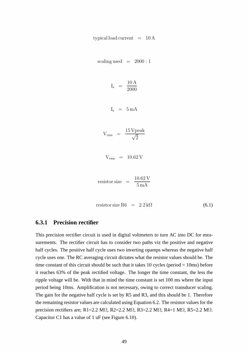
typical load current = 10 A
scaling used = 2000 : 1
Is =10 A
2000
Is = 5 mA
Vrms =15 Vpeak√
2
Vrms = 10.62 V
resistor size =10.62 V
5 mA
resistor size R6 = 2.2 kΩ (6.1)
6.3.1 Precision rectifier
This precision rectifier circuit is used in digital voltmeters to turn AC into DC for mea-
surements. The rectifier circuit has to consider two paths viz the positive and negative
half cycles. The positive half cycle uses two inverting opamps whereas the negative half
cycle uses one. The RC averaging circuit dictates what the resistor values should be. The
time constant of this circuit should be such that it takes 10 cycles (period = 10ms) before
it reaches 63% of the peak rectified voltage. The longer the time constant, the less the
ripple voltage will be. With that in mind the time constant isset 100 ms where the input
period being 10ms. Amplification is not necessary, owing to correct transducer scaling.
The gain for the negative half cycle is set by R5 and R3, and this should be 1. Therefore
the remaining resistor values are calculated using Equation 6.2. The resistor values for the
precision rectifiers are; R1=2.2 MΩ, R2=2.2 MΩ, R3=2.2 MΩ, R4=1 MΩ, R5=2.2 MΩ.
Capacitor C1 has a value of 1 uF (see Figure 6.10).
49

VoutDC = Vin AC
(
R5
R4−
R5
R3
)
(6.2)
6.4 Voltage Measured Across the Red and Blue Phases
Medium voltage measurements at power stations, for example, are typically measured
using a voltage transformer and transducer combination before sending a 4-20 mA reading
to the control desk, where the signal is converted into a voltage reading.
A LEM voltage sensor and a precision rectifier circuit are used to measure, scale and
rectify the generators line voltage, between red and blue phases, into a 0-5 V signal. This
is done so that it can be digitised by the ADC. Once the signal is digitised it can be
manipulated for transmitting.
Applying the red-and-blue phases across a 27 kΩ resistor gives rise to an input current to
the sensor of 7.5 mA. A fixed scale of 1:2.5 is applied which gives rise to an rms output
current of 18.8 mA. Passing the output current into a 566Ω resistor gives rise to 10.62
V rms or 15 V peak-to-peak. The sensor’s output voltage is fedinto a precision rectifier
circuit.
Ip =200 Vrms
27 kΩ
IPrms = 7.5 mA
scaling = 2.5 : 1
Is = 2.5 × 7.5 mA
secondary rms voltage =15 Vrms√
2
secondary rms voltage = 10.62 V
50

Figure 6.5: LV25P voltage circuit.
Figure 6.6: LAH50P current circuit.
Figure 6.7: Precision rectifier circuit.
51

Figure 6.8: LV25P voltage sensor schematic.
Figure 6.9: LAH50P current sensor schematic.
Figure 6.10: Precision rectifier schematic .
52
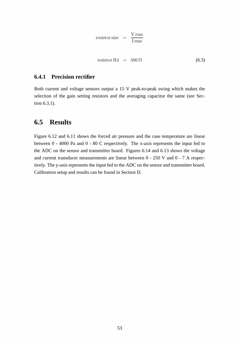
resistor size =V rms
I rms
resistor R4 = 566 Ω (6.3)
6.4.1 Precision rectifier
Both current and voltage sensors output a 15 V peak-to-peak swing which makes the
selection of the gain setting resistors and the averaging capacitor the same (see Sec-
tion 6.3.1).
6.5 Results
Figure 6.12 and 6.11 shows the forced air pressure and the case temperature are linear
between 0 - 4000 Pa and 0 - 80 C respectively. The x-axis represents the input fed to
the ADC on the sensor and transmitter board. Figures 6.14 and6.13 shows the voltage
and current transducer measurements are linear between 0 - 250 V and 0 - 7 A respec-
tively. The y-axis represents the input fed to the ADC on the sensor and transmitter board.
Calibration setup and results can be found in Section D.
53
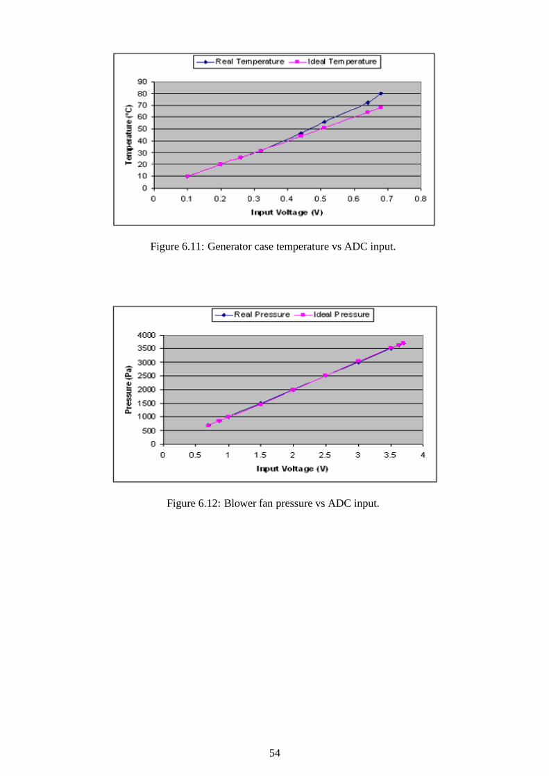
Figure 6.11: Generator case temperature vs ADC input.
Figure 6.12: Blower fan pressure vs ADC input.
54
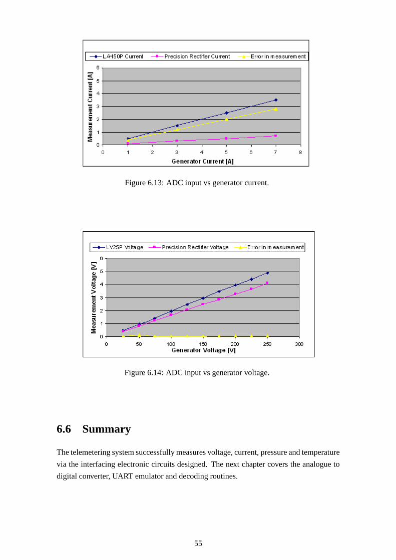
Figure 6.13: ADC input vs generator current.
Figure 6.14: ADC input vs generator voltage.
6.6 Summary
The telemetering system successfully measures voltage, current, pressure and temperature
via the interfacing electronic circuits designed. The nextchapter covers the analogue to
digital converter, UART emulator and decoding routines.
55

Chapter 7
Telemetering Software
The microcontroller software serves an early warning indication for the telemetering sys-
tem. Data is analysed from four sensors and warns the user when the system is operating
out of specification. The monitored parameters are listed inSection 1.4 point 7. Both
microcontrollers are programmed in Assembler. This chapter explains the analogue to
digital converter, UART emulator and decoding routines.
7.1 Software Design
The sensing and transmitter microcontroller (micro 1) is inthe wendy house with the
motor, generator and blower fan, whereas the receiver and display microcontroller (micro
2) are located in the Microwave Lab on the 6th floor of the Menzies Building. The flow
diagram illustrates the process of sending four parametersremotely (see Figure 7.1).
Headers 01, 02, 03 and 04 are used to separate readings in the sensor and transmitter
board’s software (see Table 7.1). A header 01 is loaded into the accumulator where it’s
placed on a stack. The stack is called up by the put_serial routine where each bit is pushed
out over PTB0. At this point the temperature sub routine is called, which selects the ADC
channel and after the conversion stores the result in the ADRregister before sending it
to the accumulator. Once the temperature reading is in the accumulator the put_serial
routine sends the byte over PTB0.
The put_serial routine is what the micro 1 uses to send a byte over the microcontroller’s
serial communication pin 15. A transmission sentence consists of 1 start bit followed by
8 data bits and a stop bit. The baud rate is set by the variable “bit delay” which stores the
period of a bit. A one second delay between calling the put_serial routine is necessary to
ensure that the receiver is waiting in the get_serial routine.
On the receiver and display board the get_serial routine waits until a header is sent from
the sensor and transmitter board. Once the header has been received the code compares
56

Table 7.1: I/O functions and allocations.Sensor and transmitter micro 1Receiver and display micro 2
Function Port Pin Function Port PinTemperature B3 12 Serial comm B0 15
Pressure D2 17 LCD D6 10Current B1 14 LCD D7 9Voltage B2 13 LCD B4 11
Serial comm B0 15 LCD B5 8Headers LCD B6 7
Temperature 01 LCD B7 6Pressure 02Current 03Voltage 04
it to the four possible headers viz, 01-04. If none of the fourheaders are received, the
code will interpret this as an error and will go to the wait fordata routine. The next byte
will most probably be sensor data, which will give an error too. On receiving the correct
header the code will exit the wait for data routine and will goto the appropriate decode
routine. This will display the result until the next header is received. Both the transmitter
and receiver loops continuously see Figure 7.1. See SectionE for the source code.
57
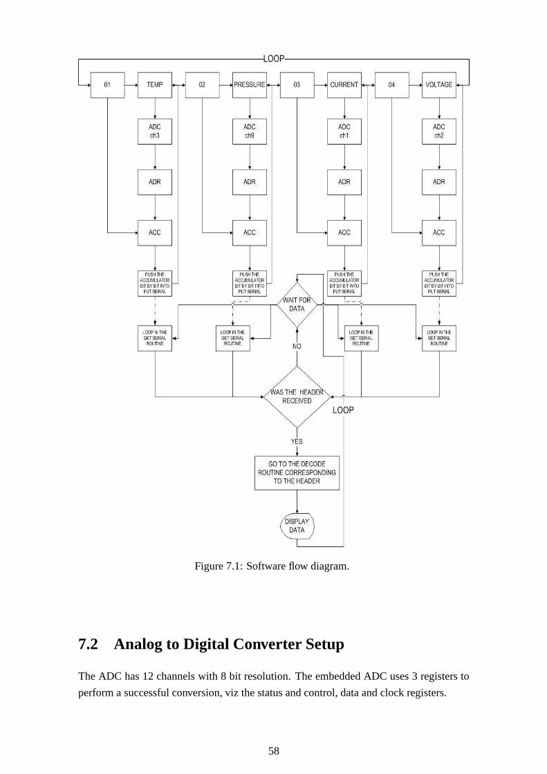
Figure 7.1: Software flow diagram.
7.2 Analog to Digital Converter Setup
The ADC has 12 channels with 8 bit resolution. The embedded ADC uses 3 registers to
perform a successful conversion, viz the status and control, data and clock registers.
58

7.2.1 Status and control register
This register chooses between continuous or single ADC conversions and which input
pins are used. After a successful conversion bit 7 is set, andcleared when conversion data
is written to the data register.
7.2.2 Data register
Each time a conversion is complete this register is updated with the 8 bit result until the
next conversion is complete and the register is overwritten.
The code lda ADR moves the result from the data register to theaccumulator.
7.2.3 Clock register
Writing to the pre-scale bits in this register selects the clock frequency used to perform a
conversion. It is recommended that ADC clock be set to 1 MHz.
7.3 Universal Asynchronous Receiver Transmitter Emu-
lator
7.3.1 Put serial
The byte sent is pushed onto HX register by the PSHX instruction. Toggling PTB0 ini-
tialises the receiver telling it that 8 data bits and a stop bit is to follow. This why the value
9 is stored in the bit count variable “X”. The carry bit is necessary as each bit is rotated
to the right until the cycle is complete. Each bit is then toggled according to each state
until the X register decrements to zero. This method of a UARTroutine is known as bit
banging. See put_serial routine below.
pshx
bclr 0,PTB ;start bit
bset 0,DDRB
sec ;initialize carry flag
ldx #9
send_loop:
jsr bit_delay
rora
bcc bitlo
bset 0,PTB
59

bra next_loop
bitlo: bclr 0,PTB
next_loop:
dbnzx send_loop
bset 0,PTB ;stop bit
jsr bit_delay ;stop bit and gaurd time
jsr bit_delay
bclr 0,DDRB ;pullup resistors hold stop state
pulx
rts
7.3.2 Get serial
The receiver stays in the wait_for_start routine until a start bit is received. The half_bit_delay
samples the PTB0 for the start bit. On receiving the start bitthe receive loop is called
where bits are checked for their status. The instructions “clc” and “sec” clears and sets
the status of the carry bit. The receive loop cycles 8 times until the variable “code” repre-
sents the transmitted byte.
pshx
bclr 0,DDRB ;serial line is input
clra
ldx #8
wait_for_start:
brset 0,PTB,wait_for_start ;wait for the start bit
jsr half_bit_delay ;sample each bit at half it’s period
receive_loop:
jsr bit_delay
brset 0,PTB,bithi
clc
bra rotate
bithi: sec
rotate: rora
dbnzx receive_loop
jsr bit_delay ;wait for stop bit
pulx
bset 0,DDRB
rts
60

7.3.3 Testing the UART on the sensor and transmitter board
To test the UART code was written whereby a pot on PTD2 was varied, the result inter-
preted by the ADC and sent to the put_serial routine. A scope probe was connected to
PTB0 and the result was captured on the oscilloscope in Figure 7.2. The result shows the
start bit, 8 data bits and the stop bit.
Figure 7.2: Bit sent over PTB0 with the sensor and transmitter board.
7.3.4 Testing the UART on the receiver and display boards
Time did not allow for testing the UART on the receiver and display board.
7.4 Transducer Scaling
The transducer resolutions were amplified as far as possiblesuch that to match the ADC
step sizes. This ensures that a small transducer increment translates to a small ADC
change as opposed to a small increment translating into a bigADC change, see Table 7.2.
Table 7.2: Sensor scaling.Sensor Sensor range ADC Channel ADC step size Scale Results
Temperature 0-150 C ADC3 20 mV 10 mV1 C
Figure 6.11, 7.3Pressure 0-4240 Pa ADC9 20 mV 20 mV
16 PaFigure 6.12, 7.4
Current 0-50 A ADC1 20 mV 20 mV200 mA
Figure 6.13, 7.5Voltage 0-250 V ADC2 20 mV 20 mV
1 VFigure 6.14, 7.6
61

7.5 Temperature Decoding
To obtain a decimal number reading from the temperature sensor input the bin method
was used. This uses three storage variables for the unit, tenand hundred positions of the
decimal number. Each time these separate bins are incremented depending if a “1” is
found. See Figure 7.3 for a temperature reading.
brclr 0,disp_no,bit1
inc units
bit1: brclr 1,disp_no,bit2
lda units
add #2
sta units
bit2: brclr 2,disp_no,bit3
lda units
add #4
sta units
bit3: brclr 3,disp_no,bit4
lda units
add #8
sta units
bit4: brclr 4,disp_no,bit5
inc tens
lda units
add #6
sta units
bit5: brclr 5,disp_no,bit6
inc tens
inc tens
inc tens
lda units
add #2
sta units
62

bit6: brclr 6,disp_no,bit7
lda tens
add #6
sta tens
lda units
add #4
sta units
bit7: brclr 7,disp_no,rollover
inc hundreds
lda tens
add #2
sta tens
lda units
add #8
sta units
7.6 Pressure Decoding [14]
The scaling has an amplification of 488. Each ADC increment isset to 16 Pa. The ADC
digital number is multiplied by 16. This bin has 4 four bin variables viz. units, tens,
hundreds and thousands. Each bit is checked see whether it isset or not. If bit 0 is set
(the decimal number equals 20 = 1) the pressure is 16 Pa. This is due to each digital
increment being 16 Pa. Therefore 6 is added to the unit bin and1 is added to the tens bin
(see Figure 7.4).
mult:
mov #$00,units
mov #$00,tens
mov #$00,hundreds
mov #$00,thous
lda #$1B ; convert pressure
cmp mult_no
beq pressure
pressure:
lda #$00
63

brclr 0,PTB,inc1
mov #$06,units
mov #$01,tens
jsr overflow
inc1: brclr 1,PTB,inc2
lda units
add #$02
sta units
lda tens
add #$03
sta tens
jsr overflow
inc2: brclr 2,PTB,inc3
lda units
add #$04
sta units
lda tens
add #$06
sta tens
jsr overflow
inc3: brclr 3,PTB,inc4
lda units
add #$08
sta units
lda tens
add #$02
sta tens
lda hundreds
add #$01
sta hundreds
jsr overflow
inc4: brclr 4,PTB,inc5
lda tens
add #$06
64

sta tens
lda tens
add #$05
sta tens
lda hundreds
add #$02
sta hundreds
jsr overflow
inc5: brclr 5,PTB,inc6
lda units
add #$02
sta units
lda tens
add #$01
sta tens
lda hundreds
add #$05
sta hundreds
jsr overflow
inc6: brclr 6,PTB,inc7
lda units
add #$04
sta units
lda tens
add #$02
sta tens
lda thous
add #$01
sta thous
jsr overflow
inc7: brclr 7,PTB,out
lda units
add #$08
sta units
lda tens
add #$04
65

sta tens
lda thous
add #$02
sta thous
jsr overflow
out: rts
7.7 Current Decoding
After a successful current conversion the ADR register stores the result in the variable
disp_no. This number is broken down into its hundreds, tens and units quantities. This
number in disp_no is divided by 100 where the quotient is placed in the accumulator
and the remainder is placed in H. The variable stores the quotient by the “sta hundred”
instruction. To obtain the tens the quotient of the first division is multiplied by a hundred
which is subtracted from the original number in disp_no. Theanswer is divided by 10
and the quotient is placed in the variable tens. Lastly the variable units are multiplied by
10 and subtracted from the original number in disp_no to obtain the units. The number is
broken into hundreds, tens and units. See Figure 7.5 for a typical current reading.
clrh ;hundreds=int(disp_no/100)
lda disp_no
ldx #$64
div
sta hundreds
mul ;disp_no=disp_no-100*hundreds
sta tens
lda disp_no
sub tens
sta disp_no
ldx #$0A ;tens=int(disp_no/10)
clrh
div
sta tens
mul ;units=disp_no-10*tens
sta units
lda disp_no
sub units
sta units
rts
66

7.8 Voltage Decoding
After a successful voltage conversion the ADR register stores the result in the variable
disp_no. This number is broken down into its hundreds, tens and units quantities. This
number in disp_no is divided by 100 where the quotient is placed in the accumulator
and the remainder is placed in H. The variable stores the quotient by the “sta hundred"
instruction. To obtain the tens the quotient of the first division is multiplied by a hundred
which is subtracted from the original number in disp_no. Theanswer is divided by 10 and
the quotient is placed in the variable tens. Lastly the variable units are multiplied by 10
and subtracted from the original number in disp_no to obtainthe units. The code jumps
to the bcd routine. See Figure 7.6 for a typical voltage reading.
clrh ;hundreds=int(disp_no/100)
lda disp_no
ldx #$64
div
sta hundreds
mul ;disp_no=disp_no-100*hundreds
sta tens
lda disp_no
sub tens
sta disp_no
ldx #$0A ;tens=int(disp_no/10)
clrh
div
sta tens
mul ;units=disp_no-10*tens
sta units
lda disp_no
sub units
sta units
rts
The typical displays can be seen in Figures 7.3, 7.4, 7.5 and 7.6.
67

Figure 7.3: Temperature display.
Figure 7.4: Pressure display.
Figure 7.5: Current display.
Figure 7.6: Voltage display.
68

7.9 Summary
The objective of this chapter was to re-use code already written by a student who pro-
grammed a monitoring unit to measure the same four parameters, however, what was
supposed to be a straight forward exercise turned out to be a time consuming debugging
exercise which could not be solved in the required time, for this project. The following
was achieved:
• The analog to digital converter is setup on four channels ports [B1-3, D2] and de-
codes the analog data in the 8 bit data register.
• The UART emulator on the sensor and transmitter board succesfully sends data.
• The UART emulator on the receiver and display board failed tointerpret the trans-
mitted sensor data via a cable.
• The decode routines were written and were tested on the sensor and transmitter
board.
69
Chapter 8
Conclusions
The goal of the project is to commission an airborne generator as a source of three phase
power at 400 Hz for ground based radar equipment at the University. The generator is
planned to be housed in a shed outside the Menzies building which shall distribute 200
V line-to-line over power cables terminating onto a 45 Amp circuit breaker located in the
microwave laboratory. The objectives were met as follows:
The induction motor chosen meets the generator’s drive end requirements for 12 kVA
operation. A cast iron coupling mechanically links the motor’s shaft to the drive end of
the generator. Starting the coupled induction motor tripped the upstream breaker. This
was due to the large startup currents inherent to induction motors, which are in the order
of 2-3 times that of rated current (see Section 3.2.1). Fortunately an off the shelf soft
starter can be used to solve this problem. Replacing the upstream circuit breaker would
be a feasible solution, however, the breaker is the propertyof the University and could not
be altered.
Soft starters reduce the voltage by a factor of1√3
in order to reduce the starting current by
the same factor, however, this reduces the torque by a factorof 13
. This created a problem
whereby the there was insufficient torque from the motor to overcome its standstill inertia
and drive the generator, as a result the motor stalled thus tripping the overload relay. This
problem was solved by using an auxiliary contact which was used to start the generator
when the motor reaches full rated conditions (see Section 4.3).
The generator and its control unit were tested according to the pre commissioning tests
provided by the technical manual and no fault was found on both items (see Section 4.4 ).
This was particularly important as the age of the generator was disconcerting. To start the
generator an external DC signal supplies a holding current of 200 mA to relay K1, which
would have been supplied by batteries onboard the aircraft,now had to be designed. A 28
Vdc power supply was designed and started the generator successfully (see Section 4.1).
This unit was used to synchronise the generator to the motor’s starter to prevent it from
stalling. A resistive load bank was used to test the generator response to various loads.
Table 4.2 summarises these results. Out of these tests two other important results were
learned. The first was the generator’s voltage decreased below its specified range when
70
it supplied loads greater than 2.2 kW. The second result was that the generator’s case
temperature reached 63 % of its maximum operating temperature under no load within
3.5 minutes.
The generator was setup according to the 12 kVA operation andwhile in this region the
amount by which the voltage and frequency should vary is between 1% - 2% respectively.
However, during tests it was shown that the voltage began to vary outside this range for
loads greater than 2.2 kW.
Onload the generator began to reach 88% of its maximum operating temperature in 3.5
minutes. So as is, the generator is of not much use. A blower fan was selected to source
forced cooling at a rate 11m3
sat 3 kPa. The cooling shroud supplies cooling air into the
inlet vents and over the gearbox housing. Forced cooling wasable to reduce and stabilise
the generator’s operating temperature while supplying a 2.2 kW and 4.8 kW loads to 45
C - 55 C respectively.
The telemetering system was designed to relay system parameters to user in the shed as
the temperature of the generator case and the blower fan pressure should not exceed 80
C and 3 kPa respectively. The voltage and current can be measured from the microwave
laboratory.
The problem of frequency hunting raised its ugly head latteron in the project whereby
the generator’s frequency oscillates between 328 and 336 Hzwhile the voltage remains at
200 V line to line. The root cause of this problem has not been investigated thoroughly;
however there are two assumptions which are addressed in Section 4.5. For this reason
the rotary inverter system should not be used.
71
Chapter 9
Recommendations
1. The 400 Hz generator is not in a state to be used as the intermittent frequency
problem could not be solved during the time allowed for this project. However,
before frequency hunting the load tests suggests that the 400 Hz generator should
not supply loads greater than 2.2 kW, as larger loads affect the voltage tolerance
negatively (see Section 4.5).
2. Further research should investigate whether the intermittent frequency hunting prob-
lem is caused by the induction motor or the generator’s constant speed drive (see
Section 4.5).
3. A pressurised pump feed should be used to replace the gearbox oil in future as an
impractical amount of force is required on the syringe as thesump fills up (see
Section 4.6).
4. The shed should be sound proofed since the noise emitted from the blower will
become problematic especially around the 6th floor level of the Menzies building.
5. The telemetering sytem works well on vero board, however,it would be more robust
for student use if it were printed onto circuit board.
6. The UART emulator was tested on the sensor and transmitterboard and the result
was that it sends data, however, time did not allow for the receiver and display board
to be tested. A final recommendation is put forward that the receiver and display
board be tested on a terminal emulator, this will assist in debugging, once solved
this will make the telemetering system fully functional.
72

Appendix A
Induction Motor
A.1 No Load Test
There are negligible differences in rotational losses between a loaded motor and one that
is not. This is why I performed the test with an unloaded shaft. The no load test gives an
indication of the rotational losses in an induction motor.
PRotational = Pinput − 3I2lineR1 (A.1)
Figure A.1: The equivalent no load circuit.
A.1.1 Methodology
Measuring the line-to-line voltage and phase current of themotor, we can manipulate the
circuit to determine parameters R1,jX1, jXm. There being no distinction in the reactive
components of the circuit jX1and jXm are lumped together to form the no load reactance
in Equation A.5.
73

Table A.1: No load test results using a three phase variac.Frequency [Hz] Voltage [V_line] Amperes [A_phase] Power [W_per phase] PF
50 59.3 2.6 132 0.91050 107.7 1.9 170 0.85050 156.3 1.7 165.2 0.64350 209.0 1.9 186 0.47350 260.0 2.3 215 0.35550 313.0 2.9 240 0.27150 363.0 3.9 286 0.20650 397.0 5.4 284 0.130
ZNL =Vphase
Iline
ZNL =397V
5.4A(A.2)
ZNL = 73.5Ω
The stator on the motor is delta connected, which implies that the phase and line-to-line
voltage are the same.
ZNL = RNL + jXNL (A.3)
We get the following from Equation A.1.
RNL =PNL
I2
RNL =284W
5.42A(A.4)
RNL = 9.7Ω
The no load power reading in TableA.1 is taken from the Chauvin Arnoux 8334 Power
Meter.
XNL =√
Z2NL − R2
NL (A.5)
XNL = 72.8Ω
These are the results from an unloaded motor shaft.
74

A.2 Locked Rotor Test
Preventing the motor-shaft from rotating implies low slip which results in a low rotor
impedance. The low rotor impedance shunts the magnetizing impedance jXm , reducing
the equivalent circuit to the figure below.
Figure A.2: The equivalent locked rotor circuit.
A.2.1 Methodology
In this test the rotor is held stationary by a G-clamp. The voltage on the three-phase
auto-transformer is slowly increased until the ammeter reads 26.6 A. In my first attempt
I assumed the auto-transformer could deliver the motor’s rated current and ended the
experiment by blowing 3, 20 Amp fuses. The fuses were replaced and the problem was
soon remedied, with the use of use of a Delta-Wye current stepup transformer. This
provided the rated 26.6 Amps to the motor.
Table A.2: The induction motor’s current values at incremental voltages.Frequency [Hz] Voltage [V] Ampere [A] Power [W] PF
50 64.2 24.9 374.6 0.40350 67.1 26.1 416.0 0.40950 67.9 26.1 425.0 0.41350 69 26.6 441.0 0.414
ZLR =V line
Iphase
ZLR =69.0V
15.4A(A.6)
ZLR = 4.5Ω
75

RLR =PLR
I21
RLR =441W
(15.4)2A(A.7)
RLR = 1.86Ω
The locked rotor impedance of (Zlr=V/I) is used to calculatethe X locked rotor impedance
XLR =√
(Z2LR − R2
LR)
XLR =√
(4.48)2 − (1.86)2 (A.8)
XLR = 4.1Ω
The parameters X1 and X2 are approximately equal in value.
XLR = X1 + X2 (A.9)
X1 =X2 = 2.05Ω (A.10)
The Equation A.11 is obtained from the no load equivalent circuit.
Xm = XNL − X1
Xm = 73.4 − 2.05 (A.11)
Xm = 71.4Ω
Calculating R2
R2 =
(
X2 + Xm
Xm
)2
× (RLR − R1)
R2 =
(
2.05 + 71.4
71.4
)2
× (1.06) (A.12)
R2 = 1.12Ω
Below are the circuit parameters for the IEEE equivalent circuit for the 15 kW induction
motor using a digital power meter.
76
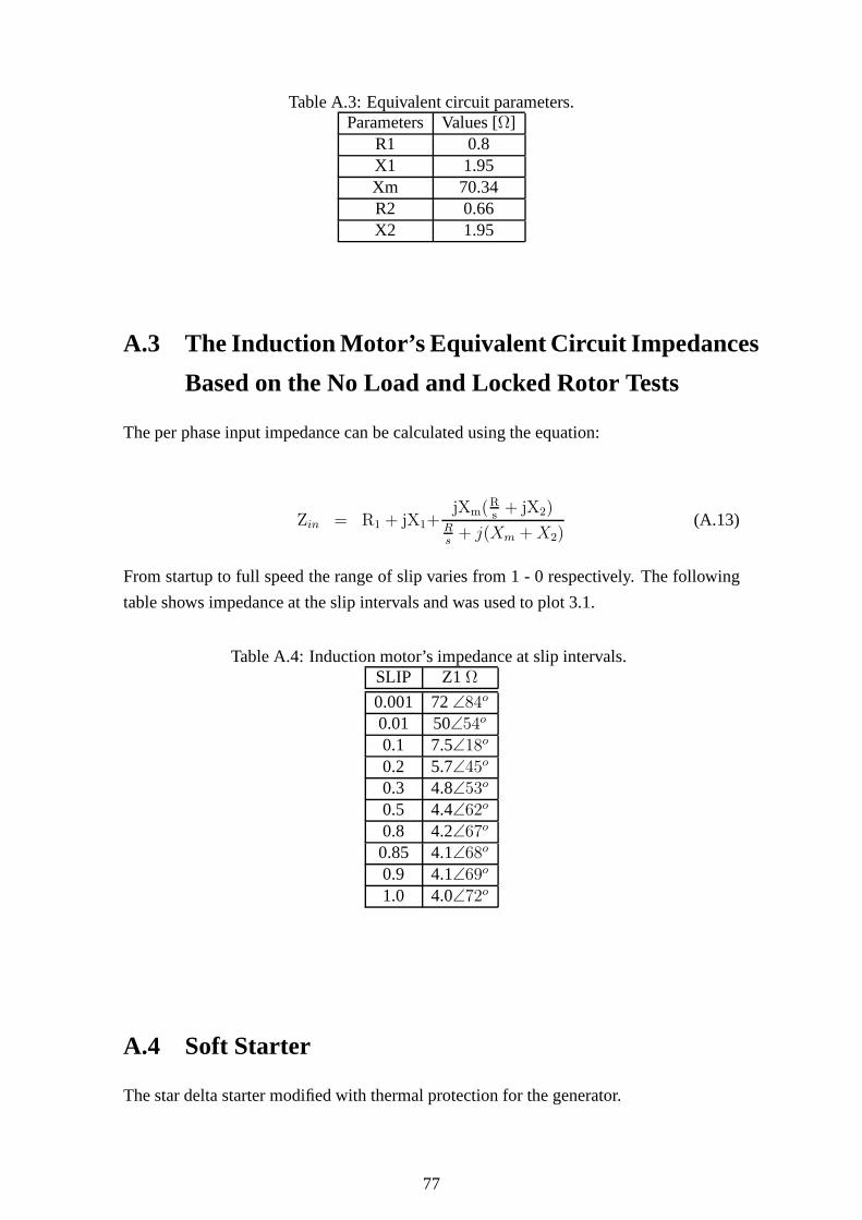
Table A.3: Equivalent circuit parameters.Parameters Values [Ω]
R1 0.8X1 1.95Xm 70.34R2 0.66X2 1.95
A.3 The Induction Motor’s Equivalent Circuit Impedances
Based on the No Load and Locked Rotor Tests
The per phase input impedance can be calculated using the equation:
Zin = R1 + jX1+jXm(R
s+ jX2)
Rs
+ j(Xm + X2)(A.13)
From startup to full speed the range of slip varies from 1 - 0 respectively. The following
table shows impedance at the slip intervals and was used to plot 3.1.
Table A.4: Induction motor’s impedance at slip intervals.SLIP Z1 Ω
0.001 72∠84o
0.01 50∠54o
0.1 7.5∠18o
0.2 5.7∠45o
0.3 4.8∠53o
0.5 4.4∠62o
0.8 4.2∠67o
0.85 4.1∠68o
0.9 4.1∠69o
1.0 4.0∠72o
A.4 Soft Starter
The star delta starter modified with thermal protection for the generator.
77

Figure A.3: Soft starter schematic.
78
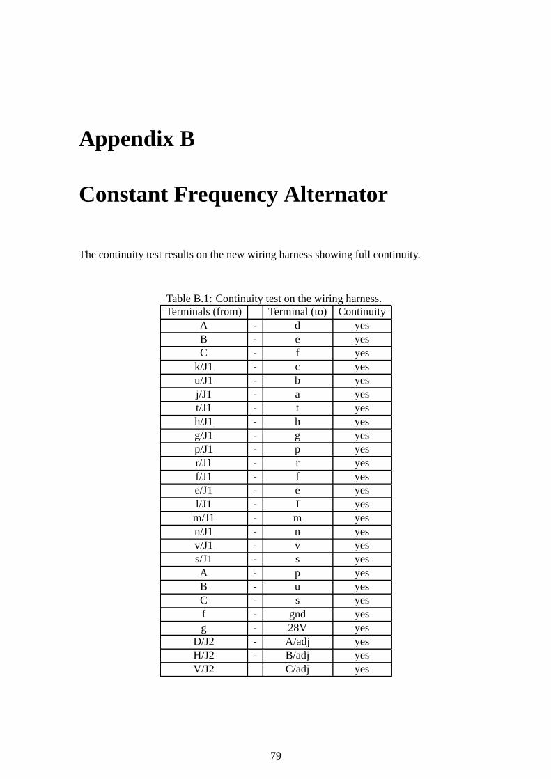
Appendix B
Constant Frequency Alternator
The continuity test results on the new wiring harness showing full continuity.
Table B.1: Continuity test on the wiring harness.Terminals (from) Terminal (to) Continuity
A - d yesB - e yesC - f yes
k/J1 - c yesu/J1 - b yesj/J1 - a yest/J1 - t yesh/J1 - h yesg/J1 - g yesp/J1 - p yesr/J1 - r yesf/J1 - f yese/J1 - e yesl/J1 - I yesm/J1 - m yesn/J1 - n yesv/J1 - v yess/J1 - s yesA - p yesB - u yesC - s yesf - gnd yesg - 28V yes
D/J2 - A/adj yesH/J2 - B/adj yesV/J2 C/adj yes
79

Appendix C
Blower Fan
C.1 Flowrate Test
This test was carried out to verify wether the fan could deliver 11 m3
sat 3 kPa. The
anemometer was kept at a distance A from the opening C. The dimensions of C are 40mm
x 30mm.
Figure C.1: The dimensions of the measuring airflow window .
C.2 Cooling Shroud Design
The cooling shroud designed in place of the ducts.
80

Figure C.2: The designed cooling shroud.
81

Appendix D
Telemetering System
D.1 The Telemetering Power Supply
A 15VA power supply was designed according to the schematic shown below.
Figure D.1: The 15 VA bipolar power supply designed for the telemetering system.
D.2 LAH50-P Calibration (Current LEM)
Equipment used for calibrating the voltage transducer:
1. Auto transformer
2. LAH50-P current transducer
3. Load Bank ( 50 - 200Ω)
4. Power supply
5. Precision rectifier (AC-DC)
D.2.1 Methodology
The resistance of the rheostat is varied which results in a changing load current, results
are recorded in Table D.1 below.
82

Figure D.2: Calibration setup for the LAH50P current transducer.
Table D.1: LAH50P calibration before and after readings using the precision rectifier at50 Hz.
Load Load Current [A] Secondary Current [mA] Full Scale Voltage [V]
1k 1 0.5 0.1500 3 1.5 0.3200 5 2.5 0.510 7 3.5 0.7
D.3 LV25P Calibration (Voltage LEM)
Equipment used in calibrating the voltage transducer:
1. Auto-transformer
2. A 50Ω load
3. LV25P voltage transducer
4. Power supply
5. Precision rectifier
D.3.1 Methodology
The auto-transformer is varied from 25 to 250 V where the loadresistance is kept fixed.
An oscilloscope measures the transducers secondary voltage and rectifiers it, and the re-
sults are shown in Table D.2 below.
Figure D.3: Calibration setup for the LV25P voltage transducer.
83

Table D.2: LV25P calibration under variable voltage at 50 Hzwith a 200Ω scaling resis-tor.
Line to line voltage [V] V rms Rectifier [V dc] ∆V
25 0.48 0.43 0.0550 0.98 0.83 0.1375 1.43 1.25 0.02100 1.97 1.65 0.03125 2.47 2.06 0.04150 2.98 2.48 0.05175 3.47 2.86 0.06200 3.95 3.26 0.07225 4.40 3.67 0.07250 4.90 4.1 0.08
84

Appendix E
Telemetering Source Code
E.1 Sensor and Transmitter Source Code
; This program reads in 4 sensor values and transmits them viathe UART of the uC
; If the sensor values exceed certain limits a shutdown operation executes and waits
; until push button 4 is pressed to begin again
TOPRAM EQU $0080 ;Top of RAM area, JK1/3=0080, JK8=0060
TOPROM EQU $F600 ;Top of Flash area JK1=F600, JK3=EC00, JK8=DC00
TOPVECTORS EQU $FFDE ;Top of Interrupt Vector table
;To calculate bit delay constants:
;Bit_del=(((crystal speed)/16)/baud rate)-5
;Half_bit_del=Bit_del/2
Bit_del EQU $5b
Half_Bit_del EQU $2d
$Include ’jl3regs.inc’
;===
org TOPRAM
temp ds 1
templ ds 1 ; temp limit
85

presl ds 1
presh ds 1
immax ds 1
ilmax ds 1
immin ds 1
ilmin ds 1
del1 ds 1
;===
org TOPROM
main:
mov #$03,CONFIG1 ; Disable the watchdog timer
mov #$0F,DDRB
mov #$00,PTB ; set data transfer line to 0
mov #$FF,DDRD
clra
clrx
clrh
bset 5,PTD ; turn on cooling system
bclr 2,PTD ; open load circuit breaker
bclr 3,PTD ; open mains circuit breaker
mov #$40,ADCLK
begin:
jsr tdelay
lda #$01
jsr put_serial
mov #$03,ADSCR ; read in temp (0-5V) on PTB bit 3
86

jsr wait_adc ; send temperature
mov ADR,temp
asl temp ; times temp by 2
lda temp
jsr tdelay
lda #$02
jsr put_serial
mov #$09,ADSCR ; read in pres (0-5V) on PTD bit 2
jsr wait_adc ; send pressure
lda ADR
jsr tdelay
lda #$03
jsr put_serial
mov #$01,ADSCR ; read in il (0-5V) on PTB bit 1
jsr wait_adc ; send load current
lda ADR
jsr tdelay
lda #$04
jsr put_serial
mov #$02,ADSCR ; read in Vm (0-5V) on PTB bit 2
jsr wait_adc ; send mains current
lda ADR
jmp begin
;===
shutdown:
jsr tdelay
87

lda #$05
jsr put_serial
bclr 5,PTD ; turn off cooling system
jsr tdelay
bset 2,PTD ; turn on load circuit breaker
jsr tdelay
bset 3,PTD ; turn on mains circuit breaker
wait
;===
wait_adc:
brclr 7,ADSCR,wait_adc
jsr tdelay
lda ADR
jsr put_serial ; send data to PTB0
rts
;===
; TIMER DELAY
;===
stdelay: mov #$05,del1 ; time delay for 5 sec
tdelay: mov #$01,del1
mov #$E1,TMODH ; time delay for 1 sec
mov #$00,TMODL
mov #$16,TSC
loop: brclr 7,TSC,loop
dbnz del1,tdelay
rts
88

;===
; SERIAL DATA TRANSFER SUB-ROUTINES
;===
;This function gets a byte of data from the serial pin of the microcontroller,
;in this case PTB0. The result is returned in the accumulator.
;Baud rate set by constants, see top of file.
;clobbers: nothing
;calls: bit_delay and half_bit_delay
get_serial:
pshx
bclr 0,DDRB ;serial line is input
clra
ldx #8
wait_for_start:
brset 0,PTB,wait_for_start ;wait for the start bit
jsr half_bit_delay ;sample each bit in the middle of its duration
receive_loop:
jsr bit_delay
brset 0,PTB,bithi
clc
bra rotate
bithi: sec
rotate: rora
dbnzx receive_loop
jsr bit_delay ;wait for stop bit
pulx
89

bset 0,DDRB
rts
;===
;This function sends a byte out over the serial pin. The inputdata
;comes in via the accumulator. Baud rate as set in constants section
;of the code.
;clobbers: nothing
;calls: bit_delay
put_serial:
pshx
bclr 0,PTB ;start bit
bset 0,DDRB
sec ;initialize carry flag to stop bit value to prevent glitches
ldx #9
send_loop:
jsr bit_delay
rora
bcc bitlo
bset 0,PTB
bra next_loop
bitlo: bclr 0,PTB
next_loop:
dbnzx send_loop
bset 0,PTB ;stop bit
jsr bit_delay ;stop bit and gaurd time
jsr bit_delay
90

bclr 0,DDRB ;pullup resistors hold stop state
pulx
rts
;===
;delay for 1 bit period. Used by the serial send and receive routines
;clobbers: nothing
bit_delay:
pshx
ldx #Bit_del
loop1: nop
dbnzx loop1
pulx
rts
;===
;delay for half a bit period. Used by the serial receieve routine
;clobbers: nothing
;branches tobit_delay
half_bit_delay:
pshx
ldx #Half_bit_del
bra loop1
;===
No_irq:
;This interrupt handler catches interrupts that happened when no
;interrupt should have occurred. For this reason the processor is halted
;and user intervention is required. This routine is only called under severe
91

;fault conditions.
stop ; Stop the processor and wait for a reset.
rti ; return
;===
org TOPVECTORS
dw No_irq ; ADC Conversion Complete interrupt
dw No_irq ; Keyboard interrupt
dw No_irq ; Unused
dw No_irq ; Unused
dw No_irq ; Unused
dw No_irq ; Unused
dw No_irq ; Unused
dw No_irq ; Unused
dw No_irq ; Unused
dw No_irq ; Unused
dw No_irq ; TIM1 Overflow interrupt
dw No_irq ; TIM1 Channel 1 interrupt
dw No_irq ; TIM1 Channel 0 interrupt
dw No_irq ; Unused
dw No_irq ; interrupt line
dw No_irq ; Software interrupt
dw main ; Reset Vector
;===
92

E.2 Receiver and Display Source Code
; This program receives code value (1-5) from UART to determine if
; temp/pres/im/ig/shutdown is sent.
TOPRAM EQU $0080 ;Top of RAM area JK1/3=0080, JK8=0060
TOPROM EQU $EC00 ;Top of Flash area JK1=F600, JK3=EC00, JK8=DC00
TOPVECTORS EQU $FFDE ;Top of Interrupt Vector table
;To calculate bit delay constants:
;Bit_del=(((crystal speed)/16)/baud rate)-5
;Half_bit_del=Bit_del/2
Bit_del EQU $5b
Half_Bit_del EQU $2d
$Include ’jl3regs.inc’
;===================================================================
org TOPRAM
comma ds 1
del1 ds 1
del2 ds 1
code ds 1
strlen ds 1 ;string display variable
lcd_temp ds 1 ;string display variable
hundreds ds 1 ;bcd decode/display variable
tens ds 1 ;bcd decode/display variable
units ds 1 ;bcd decode/display variable
thous ds 1 ;bcd decode/display variable
disp_no ds 1 ;bcd decode input argument
bcd_no ds 1
mult_no ds 1
;=========================================================
org TOPROM
main:
mov #$03,CONFIG1 ; Disable the watchdog timer
mov #$FF,DDRB ; port B outputs
mov #$00,PTB
mov #$FF,DDRD
bclr 2,DDRD ; make pot 0 - 5V available
93

bclr 3,PTD ; make sure buzzer is off
mov #$00,comma ; place a comma in LCD when set as #$FF
jsr lcd_init ; initialize the LCD module
jsr clear_lcd
ldhx #msg1 ; = LCD on
jsr lcd_string
; mov #$40,ADCLK
; mov #$29,ADSCR
display:
jsr get_serial ; get code, it determines which sensor data isgoing to be sent next
mov #$01,code
cmp code
beq disp1 ; get temperature
mov #$02,code
cmp code
beq disp2 ; get pressure
mov #$03,code
cmp code
beq disp3 ; get load current
mov #$04,code
cmp code
beq disp4 ; get mains current
mov #$05,code
cmp code
beq disp5 ; shutdown
bra display
; if code gets here then code bits not sent properly
jsr clear_lcd
ldhx #msg2 ; = Error in code
jsr lcd_string
jsr lcd_line2
ldhx #msg3 ; = transfer
jsr lcd_string
jsr tdelay
jmp display
disp4:
94

jmp disp_4 ; branch function couldn’t reach disp_4, so use jmp
disp3:
jmp disp_3 ; branch function couldn’t reach disp_3, so use jmp
disp5: ; shutdown
ldhx #msg11 ; = S-Down
jsr lcd_string
bset 3,PTD
wait
disp1: ; get tepmerature
jsr get_serial
sta disp_no
asl disp_no ; mult temp by 2 cos ADC divides by 2
jsr decode
jsr clear_lcd
ldhx #msg4 ; = Temperature
jsr lcd_string
jsr lcd_line2
jsr bcd_display
ldhx #msg5 ; = Degrees C
jsr lcd_string
jmp display
disp2: ; get pressure
jsr get_serial
sta PTB
mov #$1B,mult_no ; multiply digital no. by 1B to get BCD no.
jsr mult
jsr clear_lcd
ldhx #msg6 ; = Pressure
jsr lcd_string
jsr lcd_line2
jsr bcd_disp
ldhx #msg7 ; = Pa
jsr lcd_string
jmp display
disp_3: ; get load current
jsr get_serial
95

sta PTB
mov #$FF,comma ; insert comma on LCD
mov #$C8,mult_no ; multiply digital no. by C8 to get BCD no.
jsr mult
jsr clear_lcd
ldhx #msg9 ; = Load Current
jsr lcd_string
jsr lcd_line2
jsr bcd_display
ldhx #msg10 ; = Amps
jsr lcd_string
mov #$00,comma
jmp display
disp_4: ; get mains current
jsr get_serial
sta PTB
mov #$FF,comma ; add comma on LCD
mov #$C8,mult_no ; multiply digital no. by C8 to get BCD no.
jsr mult
jsr clear_lcd
ldhx #msg8 ; = Mains Current
jsr lcd_string
jsr lcd_line2
jsr bcd_display
ldhx #msg10 ; = Amps
jsr lcd_string
mov #$00,comma
jmp display
;==========================================================
lcd_init:
;Initialize the LCD module by turning it on, setting it into four bit
;mode, clearing the display, setting up the cursor and activating 2 line display
jsr delay1
bset 4,DDRB
bset 5,DDRB
bset 6,DDRB
96
bset 7,DDRB
bset 6,DDRD
bset 7,DDRD
mov #$32,PTB
jsr lcd_command
jsr pulse_e
jsr delay1
jsr pulse_e
jsr delay1
jsr pulse_e
jsr delay1
mov #$22,PTB
jsr lcd_command
jsr pulse_e
mov #$02,PTB ;send out the command to clear display and
;set up the cursor
jsr lcd_command
jsr pulse_e
mov #$C2,PTB
jsr pulse_e
mov #$22,PTB ;2 line etc
jsr pulse_e
mov #$82,PTB
jsr pulse_e
rts
;=========================================================
clear_lcd:
mov #$02,PTB
jsr lcd_command
jsr pulse_e
mov #$22,PTB
jsr pulse_e
mov #$02,PTB
jsr pulse_e
mov #$12,PTB
jsr pulse_e
97

rts
;==========================================================
home_lcd:
;Send the LCD cursor to the top left hand corner.
mov #$02,PTB
jsr lcd_command
jsr pulse_e
mov #$22,PTB
jsr pulse_e
rts
;==========================================================
display_char:
;Display the character in the accumulator on the LCD
psha
ora #$02
sta PTB
jsr lcd_data
jsr pulse_e
pula
nsa
ora #$02
sta PTB
jsr pulse_e
rts
;===========================================================
lcd_line2:
;Move the LCD cursor to the bottom left hand corner
mov #$C2,PTB
jsr lcd_command
jsr pulse_e
mov #$02,PTB
jsr pulse_e
rts
;==========================================================
pulse_e:
;pulse the strobe line of the LCD
98

jsr delay4
bset 7,PTD
jsr delay4
bclr 7,PTD
jsr delay4
bset 7,PTD
jsr delay4
rts
;===========================================================
lcd_command:
;clear the LCD register select line. This makes the LCD accept commands.
bclr 6,PTD
rts
;============================================================
lcd_data:
;Set the LCD register select line. This makes the LCD accept data.
bset 6,PTD
rts
;============================================================
lcd_string:
;Display a text string. The address of the string is in H:X
;The length of the string is the first character in the string
;eg ’3the’ will display ’the’
mov X+,strlen ;get the string length, increment pointer
lcd_loop: mov X+,lcd_temp
lda lcd_temp
jsr display_char
dbnz strlen,lcd_loop
rts
;============================================================
bcd_disp:
;Display a BCD number on the LCD. The number comes in in the variables hundreds,
;tens and units. an offset of $30 is added to convert the number to ASCII
lda thous
add #$30
jsr display_char
99

bcd_display: lda hundreds
add #$30
jsr display_char
lda tens
add #$30
jsr display_char
lda #$FF
cmp comma
beq addcomma
uni: lda units
add #$30
jsr display_char
rts
addcomma: ldhx #msg12 ; = ,
jsr lcd_string
jmp uni
;===========================================================
decode:
;Decode an 8 bit binary number to BCD and pack it into the variables hundreds,
;tens and units, ready for display.
clrh ;hundreds=int(disp_no/100)
lda disp_no
ldx #$64
div
sta hundreds
mul ;disp_no=disp_no-100*hundreds
sta tens
lda disp_no
sub tens
sta disp_no
ldx #$0A ;tens=int(disp_no/10)
clrh
div
sta tens
mul ;units=disp_no-10*tens
sta units
100

lda disp_no
sub units
sta units
rts
;===========================================================
; convert binary no. into "bins" of units, tens, hundreds andthous
; so they can be display on LCD
mult:
mov #$00,units
mov #$00,tens
mov #$00,hundreds
mov #$00,thous
lda #$1B ; convert pressure
cmp mult_no
beq pressure
lda #$C8 ; convert current
cmp mult_no
beq current_
current_: ; branch can’t reach current so use jmp function
jmp current
pressure: ; pressure decoding process, see chapter 3.3.4 ofthesis for explanation
lda #$00
brclr 0,PTB,inc1
mov #$06,units
mov #$01,tens
jsr overflow
inc1: brclr 1,PTB,inc2
lda units
add #$02
sta units
lda tens
add #$03
sta tens
jsr overflow
inc2: brclr 2,PTB,inc3
lda units
101

add #$04
sta units
lda tens
add #$06
sta tens
jsr overflow
inc3: brclr 3,PTB,inc4
lda units
add #$08
sta units
lda tens
add #$02
sta tens
lda hundreds
add #$01
sta hundreds
jsr overflow
inc4: brclr 4,PTB,inc5
lda tens
add #$06
sta tens
lda tens
add #$05
sta tens
lda hundreds
add #$02
sta hundreds
jsr overflow
inc5: brclr 5,PTB,inc6
lda units
add #$02
sta units
lda tens
add #$01
sta tens
lda hundreds
102

add #$05
sta hundreds
jsr overflow
inc6: brclr 6,PTB,inc7
lda units
add #$04
sta units
lda tens
add #$02
sta tens
lda thous
add #$01
sta thous
jsr overflow
inc7: brclr 7,PTB,out
lda units
add #$08
sta units
lda tens
add #$04
sta tens
lda thous
add #$02
sta thous
jsr overflow
out: rts
current: ; current decoding process
lda #$00 ;units == 1st decimal place
brclr 0,PTB,iinc1 ;tens == units
mov #$02,units ;hundreds == tens
jsr overflow
iinc1: brclr 1,PTB,iinc2
lda units
add #$04
sta units
jsr overflow
103

iinc2: brclr 2,PTB,iinc3
lda units
add #$08
sta units
jsr overflow
iinc3: brclr 3,PTB,iinc4
lda units
add #$06
sta units
lda tens
add #$01
sta tens
jsr overflow
iinc4: brclr 4,PTB,iinc5
lda units
add #$01
sta units
lda tens
add #$03
sta tens
jsr overflow
iinc5: brclr 5,PTB,iinc6
lda units
add #$03
sta units
lda tens
add #$06
sta tens
jsr overflow
iinc6: brclr 6,PTB,iinc7
lda units
add #$05
sta units
lda tens
add #$02
sta tens
104

lda hundreds
add #$01
sta hundreds
jsr overflow
iinc7: brclr 7,PTB,out
lda units
add #$01
sta units
lda tens
add #$05
sta tens
lda hundreds
add #$02
sta hundreds
jsr overflow
jmp out
;===========================================================
overflow:
; this checks if bins are >9 then increments higher bin
lda units
cmp #$0A
bcs ts ; if 10 > units then branch
sub #$0A
sta units
inc tens
ts: lda tens
cmp #$0A
bcs th ; if 10 > tens then branch
sub #$0A
sta tens
inc hundreds
th: lda hundreds
cmp #$0A
bcs te ; if 10 > hundreds then branch
sub #$0A
sta hundreds
105

inc thous
te: rts
;===========================================================
msg1:
db !6
db "LCD on"
msg2: db !13
db "Error in code"
msg3: db !8
db "transfer"
msg4: db !12
db "Temperature:"
msg5: db !10
db " Degrees C"
msg6: db !9
db "Pressure:"
msg7: db !3
db " Pa"
msg8: db !13
db "Mains current"
msg9: db !12
db "Load current"
msg10:db !5
db " Amps"
msg11:db !7
db " S-Down"
msg12:db !1
db ","
;============================================================
;delay4 = short, delay1 = intermediate and delay5 = very long
delay4:
mov #$01,del1
bra delay2
delay5:
mov #$FF,del1
bra delay2
106

delay1:
mov #$20,del1
delay2: mov #$FF,del2
delay3: nop
nop
nop
dbnz del2,delay3
dbnz del1,delay2
rts
;===========================================================
; Timer delay
;===========================================================
tdelay:
mov #$E1,TMODH ; time delay for 1 sec
mov #$00,TMODL
mov #$16,TSC
loop: brclr 7,TSC,loop
rts
;=========================================================
; SERIAL DATA TRANSFER SUB-ROUTINES
;=========================================================
;This function gets a byte of data from the serial pin of the microcontroller,
;in this case PTB0. The result is returned in the accumulator.
;Baud rate set by constants, see top of file.
;clobbers: nothing
;calls: bit_delay and half_bit_delay
get_serial:
pshx
bclr 0,DDRB ;serial line is input
clra
ldx #8
wait_for_start:
brset 0,PTB,wait_for_start ;wait for the start bit
jsr half_bit_delay ;sample each bit in the middle of its duration
receive_loop:
jsr bit_delay
107

brset 0,PTB,bithi
clc
bra rotate
bithi: sec
rotate: rora
dbnzx receive_loop
jsr bit_delay ;wait for stop bit
pulx
bset 0,DDRB
rts
;=========================================================
;This function sends a byte out over the serial pin. The inputdata
;comes in via the accumulator. Baud rate as set in constants section
;of the code.
;clobbers: nothing
;calls: bit_delay
put_serial:
pshx
bclr 0,PTB ;start bit
bset 0,DDRB
sec ;initialize carry flag to stop bit value to prevent glitches
ldx #9
send_loop:
jsr bit_delay
rora
bcc bitlo
bset 0,PTB
bra next_loop
bitlo: bclr 0,PTB
next_loop:
dbnzx send_loop
bset 0,PTB ;stop bit
jsr bit_delay ;stop bit and gaurd time
jsr bit_delay
bclr 0,DDRB ;pullup resistors hold stop state
pulx
108

rts
;=========================================================
;delay for 1 bit period. Used by the serial send and receive routines
;clobbers: nothing
bit_delay:
pshx
ldx #Bit_del
loop1: nop
dbnzx loop1
pulx
rts
;==========================================================
;delay for half a bit period. Used by the serial receieve routine
;clobbers: nothing
;branches tobit_delay
half_bit_delay:
pshx
ldx #Half_bit_del
bra loop1
;==========================================================
No_irq:
;This interrupt handler catches interrupts that happened when no
;interrupt should have occurred. For this reason the processor is halted
;and user intervention is required. This routine is only called under severe
;fault conditions.
stop ; Stop the processor and wait for a reset.
rti ; return
;=========================================================
org TOPVECTORS
dw No_irq ; ADC Conversion Complete interrupt
dw No_irq ; Keyboard interrupt
dw No_irq ; Unused
dw No_irq ; Unused
dw No_irq ; Unused
dw No_irq ; Unused
dw No_irq ; Unused
109

dw No_irq ; Unused
dw No_irq ; Unused
dw No_irq ; Unused
dw No_irq ; TIM1 Overflow interrupt
dw No_irq ; TIM1 Channel 1 interrupt
dw No_irq ; TIM1 Channel 0 interrupt
dw No_irq ; Unused
dw No_irq ; interrupt line
dw No_irq ; Software interrupt
dw main ; Reset Vector
110

Appendix F
Dismantling the 400 Hz Motor
Generator Set
1. With all circuit-breakers off disconnect the three-phase load bank from the alterna-
tor’s terminals noting the which bundles are attached to which phase of the CFA.
Note the neutral wire attached to the GCU shielding.
2. Disconnect the three-phase supply from the soft starter,motor and fan terminals.
Keeping note of the orientation. Reversing wires changes motor direction.
3. Disconnect the fan coil start signal from the auxiliary contactor attached to the delta
relay inside the soft starter.
4. Disconnect the 28 V signal line from the auxiliary contactor attached to the delta
relay.
5. Disconnect the pressure and temperature switch connections from the soft starter.
6. Remove the cooling shroud from the alternator carcass by loosening the six 8mm
bolts from the shroud lip. Remove ventilation piping and carefully compress and
store in a safe place.
7. Remove the wiring harness from the alternator and keep theside attached to the
GCU connected.
8. Wrap phase wires around the alternators aliminium frame and detach the clamp.
9. Sliding the alternator out of the motors shaft keeping theCFA in the horizontal
plane at all times. Do not knock tilt or rotate the CFA as oil displaces under these
circumstances.
10. Remove the coupling unit from the flange of the motor usinga spanner.
111

Appendix G
List of Suppliers and Budget
Table G.1: Components purchased during commissioning and company details.System Components Supplier Rand amount Year
Prime Mover Induction Motor- 15 kW Alstom 6 042,00 2003Prime Mover Soft Starter- Wye/Delta Retlaw Engineering a/o 2004
Generator 400 Hz Generator SAAF Donation a/oGenerator Amphenol Connector Saftec Sales 1 500,00 2006Ventilation Veritech Fan and Ducts Veritech 17 953,36 2005Ventilation Duct- Cooling Shroud Veritech 4 286,00 2007Monitoring Data Logger and Sensors RS Components 3 686,00 2006Monitoring LEM modules LV/LAH Denver Technology 1 036,00 2006Monitoring Thermal Switch- Bi RS Components 193,06 2006Monitoring Pressure Switch- Low RS Components 243,17 2007
Total 34 939,59 2007
112
Bibliography
[1] Avions Marcel Dassault and Breguet Aviation. (1985). Generator and Regulator
Manual Technical Manual.
[2] Zyambo, J. (2004). Commissioning a 400 Hz Power Supply: Final year project,
Department of Electrical Engineering, University of Cape Town.
[2] Smith, W.A. (2005). Commissioning a 400 Hz Power Supply:Technical Report,
Department of Electrical Engineering, University of Cape Town.
[3] Yoon, J.N. (accessed 2008). 400 Hz Electrical Systems, web page,www.
aerospaceweb.org/question/electronics/q0219.shtml
[4] ABB South Africa. (2000). Commissioning procedures forthree phase induction
motors, Application Note.
[5] Wild, T.W. (1996). Transport Category Aircraft Systems, Jeppeson Sanderson Pub-
lishers Inc, ISBN 0-884875-232-7, Chapter 4.
[6] Dishner, B. and Morris, A. (1989). A novel electromechanical approach to constant
frequency power generation. Proceedings of the IEEE 1989 National Aerospace
Electronics Conference (NAECON 1989). Volume 4, pp 1765 - 1769.
[7] Taha, M. and Trainer, D.R. (2004). Adaptive reactive power control for aircraft ap-
plications. Second International Conference on Power Electronics, Machines and
Drives (PEMD 2004). (Conf. Publ. No. 498), Volume 2, pp 469 - 474.
[8] Sen, P.C. (1997). Principles of Electric Machines and Power Electronics, 2nd Edi-
tion. Wiley Publishers. ISBN 978-0-471-02295-4. Chapter 5: Asynchronous Ma-
chines, pp 222 - 247.
[9] Sen, P.C. (1997). Principles of Electric Machines and Power Electronics, 2nd Edi-
tion. Wiley Publishers. ISBN 978-0-471-02295-4. Chapter 6: Synchronous Ma-
chines, pp 292 - 365.
[10] Motorola Inc. (1997). Three Terminal Positive VoltageRegulators. Datasheet,
MC7800D.
[11] ST Microelectronics. (2004). Negative Voltage Regulators. Datasheet, L7900.
113

[12] ST Microelectronics. (2001). Low Power J-FET Quad Operational Amplifiers.
Datasheet, TL064.
[13] Radiometrix. (2004). UHF FM Data Transmitter and Receiver Modules. Datasheet,
TX2-433-160-5V/ RX2-433-160-5V.
[14] Browne, D. (2005). Generator Status Monitoring Unit. Final year project, Depart-
ment of Electrical Engineering, University of Cape Town.
[15] National Semiconductor. (2000). Precision Centigrade Temperature Sensor.
Datasheet, LM35DZ.
[16] LEM. (2003). Current Transducer. Datasheet, LAH 50-P.
[17] LEM. (2003). Voltage Transducer. Datasheet, LV25-P.
[18] RS Components. (1999). Pressure Transducer. Datasheet, 288-8533.
[19] Moeller. (2004). Motor Control Star Delta Starter. Product Catalog.
[20] Alstom. (2007). Centrifugal Fans Radial Bladed Fans. Product Catalog.
[21] Ferranti . (1975). Blue Parrot Radar S.A. , Technical Manual for the South African
Defense Force.
[22] Zyambo, J. (2004). Commissioning a 400 Hz Power Supply.Thesis disseration, De-
partment of Electrical Engineering, University of Cape Town. pp 58-59.
[23] Telemecanique. (2000). Variable Speed Drive Altivar 30 kW. pp 10-13.
[24] SABS IEC 60034-1. (1985). Rotating electrical machines. Part 1, Rating and perfor-
mance.
[25] SABS IEC 60034-2A. (1991). Rotating electrical machines. Part 2A, Methods of
determining losses and efficiency.
[26] SABS IEC 60034-5. (1972). Rotating electrical machines. Part 5, Classification of
degrees of protection provided by enclosures of rotating electrical machines.
[27] SABS IEC 60034-6. (1972). Rotating electrical machines. Part 6, Methods of cool-
ing.
[28] SABS IEC 60034-7. (1992). Rotating electrical machines. Part 7, Classification of
types of construction and mounting arrangements.
[29] SABS IEC 60034-8. (1972) Rotating electrical machines. Part 8, Terminal markings
and direction of rotation of rotating machines.
114

[30] SABS IEC 60034-12. (1980). Rotating electrical machines. Part 12, Starting per-
formance of single speed three-phase cage induction motorsfor voltages up to and
including 660 V.
[31] SABS 1804-2. (1999). Rotating electrical machines. Part 2, Low voltage three-phase
standard motors.
[33] Avions Marcel Dassault - Breguet Aviation. (1985). Generator and Regulator Tech-
nical Manual. Section 6.1.3: Products required for periodic maintenance operations,
pp 6-2.
[34] Avions Marcel Dassault - Breguet Aviation. (1985). Generator and Regulator Tech-
nical Manual. Section 9.2: Oil draining and filling, pp 9-2 - 9-3.
[35] Avions Marcel Dassault - Breguet Aviation. (1985). Generator and Regulator Tech-
nical Manual. Section 0: Characteristics, pp 00-12 - 00-13.
[36] Johan. (2005). Veritech Ventilation Systems. In conversation regarding the place-
ment of pressure sensors.
[37] Imphotonics Company. (accessed 2006). lmphotonics Systems. Motor starters,
star delta, web page,http://www.lmphotonics.com/m_start.htm#
StarDelta
115