commitment vs. discretion in the uk: an empirical ... bache, brubakk, and maith (2010) for norges...

Commitment vs. Discretion in the UK:An Empirical Investigation of the Monetary

and Fiscal Policy Regime∗

Tatiana Kirsanovaa and Stephanus le Rouxb

aUniversity of GlasgowbDepartment for Work and Pensions

This paper investigates the conduct of monetary and fiscalpolicy in the post-ERM period in the United Kingdom. Usinga simple DSGE New Keynesian model of non-cooperative mon-etary and fiscal policy interactions under fiscal intraperiodleadership, we demonstrate that the past policy in the UnitedKingdom is better explained by optimal policy under discre-tion than under commitment. We estimate policy objectives ofboth policymakers. We demonstrate that fiscal policy plays animportant role in identifying the monetary policy regime.

JEL Codes: E52, E61, E63.

1. Introduction

It has long been known in the literature on monetary policy that ifpolicymakers can precommit to a stabilization plan, then they canachieve a significant welfare gain. This is relative to the case of dis-cretionary policy and in an environment where the current decisions

∗We are grateful to Julia Darby, Campbell Leith, Jim Malley, IoannaMoldovan, and in particular three anonymous referees and the editor for use-ful suggestions and discussions. Any views expressed are solely those of theauthors and so cannot be taken to represent those of the Department for Workand Pensions or the Government of the United Kingdom or to state Depart-ment for Work and Pensions or Government of the United Kingdom policy. Allerrors remain ours. Author contact: Kirsanova: Economics, Adam Smith Busi-ness School, Gilbert Scott Building, University of Glasgow, Glasgow G12 8QQ;e-mail: [email protected]. Le Roux: Caxton House, 6-11 TothillStreet, London, SW1H 9NA; e-mail: [email protected].

99

100 International Journal of Central Banking December 2013

of the forward-looking private sector are largely determined by theirexpectations.1

A policymaker who can commit chooses a policy plan once andthen follows this policy at all dates in the future. This policy is thebest from today’s perspective, provided that the precommitment iscredible. However, the policy is time inconsistent, and with the pas-sage of time the policymaker will have an incentive to renege. Onlya policymaker whose promises are perfectly credible can precommit.

In contrast, a discretionary policy is time consistent and, as such,is perfectly credible. It is known that the policymaker reoptimizesevery period. In the resulting equilibrium, given an opportunity torenege on the expected policy for the next period, the policymakerwill find it optimal to choose the same policy for that period. Theprivate sector believes all promises, as there are no incentives torenege on them.

A credible commitment policy is able to take advantage of theforward-looking behavior of the agents by allowing them to under-stand how the policy will react to all circumstances in future periods.It can be formulated in terms of a contingent intertemporal plan, andthe plan is linked to the initial date and has clear relations betweenconsequent periods. This reflects the ability of the policymaker tomanipulate the expectations in a desired way and convince the pri-vate sector to coordinate at the best possible intertemporal outcome,linked to the date of precommitment. In contrast, a discretionarypolicy can rather be described as a set of intratemporal contingentrules; the forward-looking private sector recognizes this feature andalso reacts optimally, but it reacts only to the current state, as pastpromises are ignored.

Although the different properties of these two benchmark poli-cies having been known for decades, the issue of practical imple-mentation of such policies remains controversial. Most discussionsconcern monetary policy. Although there is little doubt that majorcentral banks are able to precommit to a target—as, for example, aninflation target—the way they actually manage the expectations ofpolicies to achieve the target remains underexplored. The key prob-lem with the acceptance of the theoretical concept of commitment

1See Kydland and Prescott (1977), Currie and Levine (1993), and Woodford(2003a), among many others.

Vol. 9 No. 4 Commitment vs. Discretion in the UK 101

policy as a practical option has always been its time inconsistency.It is well understood that the policymaker will have an incentive torenege at every consequent period. This is because the private sec-tor will have done part of the “work” of the policymaker by settingits expectations in a particular way. From this perspective the poli-cymaker would gain from exploiting the expectations of the privatesector. Also, it is because the policymaker may have some additionaland sudden “distractions,” like the task of maintaining financial sta-bility. Issues with financial stability may require sudden monetaryloosening regardless of the inflation record at the time.

Despite the well-understood difficulties with the ability of a centralbank to precommit to a policy plan, the statements of major centralbanks about their practices differ widely. The early statements do notsuggest that banks precommit to a plan which is chosen once and for-ever. In particular, after the Bank of England gained its independence,King (1997) proclaimed a regime of “constrained discretion.” In thesestatements the word “discretion,” which does not typically assume anability to manipulate expectations over time, has rather been used toacknowledge inevitable “distractions.” On the other hand, the word“constrained”wasmeant tomean that the“distractions”will notdom-inate. The Bank of England would, therefore, not pursue a short-termgain at the expense of mid-term inflation stability. This was meant toimprove the credibility of the policy in the eyes of the private sector.Nothing in King (1997) suggests that the word “discretion” is meantto exclude the possibility that the Bank of England would not be ableto manipulate the private sector’s expectations and use informationfrom a longer period of time rather than just within the current period.Bernanke and Mishkin (1997) give similar arguments to describe theU.S. monetary policy as discretionary. Coroneo, Corradi, and SantosMonteiro (2012) andGivens (2012) estimate that theVolker-Bernankeperiod in the United States is best described by the discretionary mon-etary regime.

More recently, the statements of some European central bankshave either described their current monetary policy as policy undercommitment or have come very close to doing so. The intertem-poral feature of a commitment policy is being communicated as a“predictable response pattern.” See Bergo (2007) for the view of theNorges Bank and Svensson (2009) for policy recommendations forthe Riksbank to follow in the footsteps of Norges Bank by generating


policy projections as optimal projections. Using medium-scale macromodels, Bache, Brubakk, and Maith (2010) for Norges Bank andAdolfson et al. (2011) for the Riksbank, find that the past policy ofthese banks is better explained as optimal policy under commitmentthan as simple rules.

The recent documents may imply that the Bank of England takesa similar view on the issue (Tucker 2006; Stockton 2012). A cleartarget and a public commitment to anchor inflation expectations inline with this target, together with being understood to be willing todo whatever is necessary to achieve this goal, not just in the currentperiod but in all periods, is critical to achieving credibility. Oncecredibility is achieved, a central bank that wants to maintain thecredibility of its promises would then clearly recognize that renegingon past promises would lead to a loss of credibility. One might inter-pret this statement as indicating that, in effect, the Bank of Englandwas able to precommit to the policy and then chose not to renege onits previously chosen intertemporal policy. It is an empirical ques-tion, however, whether the Bank of England was able to manage theprivate sector’s expectations as if the Bank could not renege on itspromises under any circumstances.

Fiscal policy arrangements are much less discussed in the liter-ature, although they may play an important role in identifying themonetary policy regime as well as parameters of the model. Partlybecause of institutional arrangements, it is believed that fiscal policyis too inflexible to be used for active stabilization. However, recentdevelopments in the world, recent episodes of using fiscal policy as astabilization device, have shown that there might be a more activerole for fiscal policy.2 A more focused discussion on the institutionaldesign of stabilizing fiscal policy may not be too far into the future.

The main focus of this paper is the identification of the degreeof policy precommitment in the United Kingdom. We work with thestandard microfounded model of a small open economy.3 We use

2Recent examples include the Economic Stimulus Act of 2008 and the Amer-ican Recovery and Reinvestment Act of 2009 in the United States, and theestablishment of the Office of Budget Responsibility in the United Kingdom. SeeOsborne (2008); see also Wyplosz (2005) and Kirsanova, Leith, and Wren-Lewis(2006) for a more formal discussion.

3We build on models in Galı and Monacelli (2005, 2008), Lubik andSchorfheide (2006, 2007), and Justiniano and Preston (2010a, 2010b).


the theoretical framework of non-cooperative monetary and fiscaldiscretionary interactions, as in Fragetta and Kirsanova (2010) andBlake and Kirsanova (2011), and we also develop the appropriatetheoretical framework for non-cooperative commitment. The policy-makers are assumed to minimize the microfounded social welfare lossfunction except that they can change the relative weight on infla-tion stabilization and introduce an additional penalty on the excessvolatility of policy instruments. We estimate structural parametersof the model and weights of policy objectives under two alterna-tive assumptions about the policymakers’ degree of precommitmentusing the Bayesian approach (see, e.g., An and Schorfheide 2007).

We demonstrate that the monetary and fiscal policy regime inthe United Kingdom under the assumption of fiscal leadership canbest be described by a regime of optimal policy under discretion:the probability that the actual data were generated by a model withoptimal commitment policy, rather than by a model with optimaldiscretionary policy, is less than 1.0 percent. Both policymakers puta smaller weight on inflation stabilization than is socially optimal,and the fiscal policymaker pays much less attention to inflation sta-bilization than the monetary policymaker. We assess the empiricalfit of an optimizing microfounded model based on first- and second-order moments and use DSGE-VAR methodology (Del Negro andSchorpfheide 2004) to investigate the degree of misspecification ofthe model under different policies. In particular, we show that theDSGE model imposes useful restrictions to improve the in-samplepredictive properties of the Bayesian VAR model. Finally, we demon-strate that the fiscal solvency constraint plays an important role asan identifying restriction for both fiscal and monetary policy reac-tions as well as model parameters: excluding the fiscal block fromthe system leads to a greater degree of misspecification of the puremonetary model.

The focus of this paper is different from the one of Fragetta andKirsanova (2010). We identify the degree of policy precommitment,while Fragetta and Kirsanova (2010) identify the degree of leadershipand work with a discretionary model only.4 Unlike Givens (2012), we

4In contrast to the model in Fragetta and Kirsanova (2010), our modelaccounts for habit persistence and inflation inertia.


use a microfounded model, and account for non-cooperative mone-tary and fiscal policy interactions, which allows a more completedescription of the UK macroeconomic policy regime. Finally, incontrast to Fragetta and Kirsanova (2010) and Givens (2012), weprocess the data in a different way: following Lubik and Schorfheide(2006), we introduce a non-stationary worldwide technology shockwhich substantially reduces the model misspecification.

This paper is organized as follows. In the next section we outlinethe model and describe policy interactions under commitment anddiscretion. Section 3 explains the empirical methodology, the choiceof priors, and the data. The results are discussed in section 4, andsection 5 concludes. Appendices contain details of derivations andthe theoretical framework for the two policy regimes in a generalrational expectations linear-quadratic framework.

2. The Model

We build on models by Galı and Monacelli (2005, 2008), Lubik andSchorfheide (2006, 2007), and Justiniano and Preston (2010a, 2010b)modified to include fiscal policy. The following section presents keystructural equations of a small open-economy model, which allowsfor habit formation and price indexation.

2.1 Households

The economy is populated by a unit-continuum representativehousehold, by a unit-continuum monopolistically competitive firm,and by two policymakers: the government and the central bank.

Each household k maximizes the following objective:

W = Et

∞∑t=0

βt

((Xk

t /AWt)1−σ

1 − σ+ χ

(Gt/AWt)1−σ

1 − σ− Nt

1+ϕ

1 + ϕ

). (1)

Here Xkt = Ck

t −hκCt−1 is the habit-adjusted consumption, Ct−1 ≡∫ 10 Ck

t−1dk is the cross-sectional average of consumption, Nt is laborsupply of a representative household, and Gt is consumption ofpublic goods. Parameter 0 ≤ h ≤ 1 measures the degree of habitpersistence, parameter β is the household discount rate, ϕ is theelasticity of labor supply, and σ is the coefficient of relative risk


aversion. Parameter χ is the scaling factor for the utility of con-suming public goods. In order to guarantee that the model has abalanced growth path, we assume that households derive utility fromeffective consumption relative to the worldwide level of technology,AWt. The technology shock AWt is non-stationary, with growth ratezt = AWt/AWt−1. Parameter κ is the steady-state value of zt.

Household k’s consumption, Ckt , is an aggregate of the contin-

uum of goods i ∈ [0, 1] produced in the home country (indexed H)and abroad (indexed F ),

Ct =(

(1 − α)1η C

η−1η

Ht + α1η C

η−1η

Ft

) ηη−1

,

where 0 ≤ α < 1 is the import share and η > 0 is the intratempo-ral elasticity of substitution between home and foreign consumptiongoods. CH is a composite of domestically produced goods given by

CHt =(∫ 1

0CHt(z)

ε−1ε dz

) εε−1

, (2)

where z denotes the good’s type or variety and ε is the intratem-poral substitution between domestically produced goods. Similarly,the aggregate CFt is an aggregate across overseas countries i,

CFt =(∫ 1

0C

ε−1ε

it di

) εε−1

,

where Cit is an aggregate similar to (2). Households allocate aggre-gate expenditures based on the demand functions:

CHt = (1 − α)(

PHt

Pt

)−η

Ct and CFt = α

(PFt

Pt

)−η

Ct,

where PHt, PFt are domestic and foreign goods price indices and

Pt =((1 − α)P 1−η

Ht + αP 1−ηFt

) 11−η

is the consumption-based price index.


Consumers face the following aggregated budget constraint:

PtCkt + Et{Qt,t+1A

kt+1} = Ak

t + (1 − τt)(WtN

kt + Υk

t

)+ Tt,

where Akt+1 is the nominal payoff of portfolio held at the end of

period t, Wt is wages, τt is the income tax rate, Υ is profits, and Tt islump-sum transfers paid by the government. Qt,t+1 is the stochasticdiscount factor for one-period-ahead payoffs.

In the maximization problem, households take the processes forCt−1, Wt, Tt, and the initial asset position Ak

−1 as given. The opti-mization produces the standard first-order conditions

11 + it

= βEt

(PtAWt

Pt+1AWt+1

(Xt/AWt

Xt+1/AWt+1

)σ)(3)

Wt

Pt= AWt

(Xt/AWt)σ

Ntϕ

(1 − τt), (4)

where 1 + it = (Et{Qt,t+1})−1 is the gross return on a riskless one-period bond paying off a unit of domestic currency in period t + 1.We omit superscript k, as all households are identical.

2.2 Firms

Domestic differentiated goods are produced by monopolisticallycompetitive firms, which use labor as the only factor of production.The production technology is given by

Yt (i) = AWtAHtNt (i) , (5)

where Yt (i) is the amount of output produced by firm i in periodt, Nt (i) is the amount of labor employed by firm i in period t, andAHt is the home-specific stationary technology shock.

We assume the familiar Calvo-type price setting (Calvo 1983). Afirm will not reset the price the next period with given probabilityθ. When firm i does not reset price, the price is costlessly adjustedwith steady-state rate of inflation Π. When firm i resets price, withprobability 1 − ζ it chooses price P f

Ht, which maximizes

maxP f

Ht(i)

∞∑k=0

θkQt,t+k

(Yt+k (i) P f

Ht (i) Πk − Wt+kNt+k (i))


subject to demand system

Yt+k (i) =[pHt (i) Πk

PHt+k

]−ε

Yt+k

and production function (5). The solution to this optimization prob-lem is given by

P fHt

PHt=

ε

ε − 1K1t

K2t, (6)

where K1t and K2t satisfy

γβK1t+1

(PHt+1

ΠPHt

)ε

= K1t −(

Xkt

AWt

)−σYt

AWt

Wt

PtAWtAHt, (7)

γβK2t+1

(PHt+1

ΠPHt

)ε−1

= K2t −(

Xkt

AWt

)−σPHt

Pt

Yt

AWt. (8)

When a firm resets price, then with probability ζ it chooses thenew price P b

Ht according to a simple rule of thumb

P bHt = P ∗

Ht−1ΠHt−1, (9)

where the index of the reset prices P ∗t−1 is given by

P ∗1−εHt = (1 − ζ)

(P f

Ht

)1−ε

+ ζ(P b

Ht

)1−ε. (10)

With share θ of firms keeping last period’s price and share (1 − θ) offirms setting a new price, the law of motion of aggregate price indexPHt is

P 1−εHt = (1 − θ) (P ∗

Ht)1−ε + θ (ΠPHt−1)

1−ε. (11)

Finally, the evolution of price dispersion Δt =∫ 10 (pHt(i)

PHt)−εdi is given

by

Δt = (1 − θ) (1 − ζ)

(P f

Ht

PHt

)−ε

+ (1 − θ) ζ

(P b

Ht

PHt

)−ε

+ θ

(PHt

PHt−1

)ε

Δt−1. (12)


2.3 Risk-Sharing, Market Clearing, and Private-SectorEquilibrium

The bilateral terms of trade measure foreign country goods pricesrelative to home goods prices. The effective terms of trade St aregiven by

St =PFt

PHt,

and the real exchange rate Qt is defined as

Qt =P ∗

t Et

Pt,

where Et is the nominal exchange rate. Assuming that the homecountry is small and the law of one price holds, we obtain

St ≡ PFt

PHt=

P ∗t Et

PH,t=

Pt

PH,t

P ∗t Et

Pt=

Pt

PH,tQt.

The Euler equation for the rest of the world can be written as

11 + i∗t

= βEt

(X∗

t /AWt

X∗t+1/AWt+1

)σ (P ∗

t

P ∗t+1

).

Combining two consumption Euler equations with the uncoveredinterest rate parity

1 + it1 + i∗t

=Et+1

Et

yields the international risk-sharing relationship

Xt/AWt

X∗t /AWt

Q− 1σ

t =Xt+1/AWt+1

X∗t+1/AWt+1

Q− 1σ

t+1.

Goods market clearing requires

Yt(j) = CHt(j) +∫ 1

0Ci

t(j)di + Gt(j),


where

CiHt(j) = α

(PHt(j)PHt

)−ε (PHt

EitP it

)−1

Cit .

The allocation of government spending across goods is determinedby the minimization of total costs,

Gt(j) =(

pHt(j)PHt

)−ε

Gt.

Substituting everything into the market clearing condition yields

Yt(j) =(

PHt(j)PHt

)−ε [(1 − α)

PtCt

PHt+ α

∫ 1

0

EitPit C

it

PHtdi + Gt

].

Aggregation, using Yt = (∫ 10 Yt(j)

ε−1ε dj)

εε−1 , yields the aggregate

demand equation

Yt = (1 − α)Pt

PHtCt + αC∗

t + Gt. (13)

Similarly, aggregation of production function (5) yields the aggregateproduction function

Yt = AWtAHtNt

Δt. (14)

We assume that all public debt consists of riskless one-periodbonds. Therefore, the nominal value of end-of-period public debt Bt

evolves according to the following law of motion:

Bt = (1 + it−1) Bt−1 + PHtGt − τtPHtYt. (15)

For analytical convenience, we define Bt = (1+it−1)Bt−1Pt−1AW t

as a measureof real government debt. Because AWt and Bt are observed at thebeginning of period t, equation (15) can be rewritten as

Bt+1AWt+1

AWt= (1 + it)

(Bt

PHt−1

PHt− τt

Yt

AWt+

Gt

AWt

). (16)

Finally, the private-sector equilibrium { Xt

AW t, Wt

Pt, Nt, Yt, K1t,

K2t, pfHt, P b

t , P ∗t , Πt, Δt, Bt} is determined by equations (3), (4),

(6), (7), (8), (9), (10), (11), (12), (13), (14), and (16).


2.4 Linearization

We proceed by log-linearizing the model equations around thebalanced growth path. Our model imposes common steady-statereal interest rates, inflation rates, growth rates, and technologies.Because the model contains a non-stationary component, the world-wide technology shock AWt, we detrend the affected variables bytheir specific growth components beforehand.

We denote by lowercase letters the stationary transformation ofcorresponding variables, by dividing them by a common numeraire,AWt. Therefore, we denote xt = Xt

AW t, yt = Yt

AW t, gt = Gt

AW t,

ct = Ct

AW t. We present the model in a form where all variables are

in log-deviations from the steady state, and for any variable ut withsteady state u we denote ut = log

(ut

u

).

The linearized system which describes the evolution of the econ-omy can be written as

πHt = βθ

ΦEtπHt+1 +

ζ

ΦπHt−1 (17)

+λ

Φ

(σxt + ϕyt + αSt − (ϕ + 1) AHt

)+ ηπt

xt = Etxt+1 − 1σ

(ıt − EtπHt+1 + αSt − αEtSt+1 − Etzt+1

)(18)

St =σ

(1 − h) (1 − α)(ct − hct−1 − c∗

t + hc∗t−1

)(19)

xt =1

(1 − h)(ct − hct−1) +

h

(1 − h)zt (20)

yt = α (2 − α) ηSt + (1 − α)ct + αc∗t +

g

cgy

t (21)

bt+1 =1β

(bt − B

yΠπHt +

g

ygy

t −(

τ − g

y

)yt

)+

B

yΠıt − B

yΠEtzt+1

(22)

Ψt = yt − yt−1 + zt (23)

Ωt = gyt − gy

t−1 + ηgt. (24)

Here gyt = gt − yt is spending-to-output ratio, or the government

share, and bt = ByΠ log

(Bt

B

)is a measure of real debt. Variables


Ψt and Ωt are the growth rate of output and of the governmentshare correspondingly. Parameters are Φ = ζ + θ − ζθ + θβζ,λ = (1 − θ) (1 − θβ) (1 − ζ). All microfounded shocks are assumedto follow an AR(1) process:

AHt = ρaAHt−1 + ηat (25)

c∗t = ρcc

∗t−1 + ηct (26)

zt = ρz zt−1 + ηzt, (27)

where ηat, ηct, and ηzt are i.i.d. Note that additional to three micro-founded shocks, AHt, zt, and c∗

t , we have added shocks ηπt and ηgt

into the final specification of the system. Shock ηπt captures ineffi-cient variations in markups. It is assumed to be i.i.d. to allow easieridentification of the degree of inflation inertia. Shock ηgt capturesthe non-systematic part of fiscal policy, the discrepancy between theobserved government share and the unobservable policy instrument.As a measurement error, ηgt is assumed to be i.i.d.

2.5 Policy

2.5.1 Social Welfare

The aggregated household utility (1) implies the following socialwelfare loss function:

W = Et

∞∑t=0

βt

(π2

Ht +ζ

θ (1 − ζ)(πHt − πHt−1)

2

+ L(xt, ct, yt , gy

t , AHt, c∗t , c

∗t−1

)),

where L(xt, ct, yt , gyt , AHt, c

∗t , c

∗t−1) is a collection of quadratic terms

which can be rearranged to describe “gap” targets; see appendix 1.

2.5.2 Policy Objectives

It is often suggested that realistic policymakers are not benevolent.There are some theoretical reasons for introducing additional objec-tives and for distorting social weights of a discretionary policymaker.A discretionary monetary policymaker can reduce the “stabilization


bias”5 in several ways. For example, Woodford (2003b) demonstratesthat if the discretionary monetary policymaker adopts an additionalinterest rate smoothing target, then the policy becomes “historydependent” and the dynamics of the economy under discretion issimilar to the one under commitment policy, with a higher level ofsocial welfare attained. A similar result is demonstrated in Vestin(2006): introducing the price-level target into the monetary policy-maker’s objectives improves the social welfare too. Also, followingthe famous result of Barro and Gordon (1983), Clarida, Galı, andGertler (1999) show that the discretionary monetary authority whichputs higher than socially optimal weight on the inflation stabiliza-tion target can achieve the same level of welfare as under the optimalprecommitment-to-rules policy.6

The policymakers may not be benevolent because of some insti-tutional restrictions, both under commitment and discretion. Forexample, fiscal instrument smoothing may result from fiscal policybeing “delayed.” All spending decisions should pass the Parliamentscrutiny. In order to avoid large changes in inappropriate times, itmay be optimal to propose only relatively small changes. In ourframework, such policy can be described by introducing a penaltyon the change of fiscal instrument. Similarly, a debt target can reflectsome international agreements. It can also help to avoid large riskpremiums, which cannot be described by this model.

To account for possible delegation schemes and institutionalrestrictions, we assume a more general form of the monetary pol-icymakers’ objective function in our empirical part of the paper:

WM = Et

∞∑t=0

βt

(ΦπM

(π2

Ht +ζ

θ (1 − ζ)(πHt − πHt−1)

2)

+ L(xt, ct, yt , gy

t , AHt, x∗t , c

∗t

)+ ΦΔI (Δıt)

2)

.

Here we add additional interest rate smoothing weight ΦΔI and allowfor “inflation conservatism” ΦπM .

5See Svensson (1997).6For other policy delegation proposals, see, e.g., Svensson (1997), Walsh

(2003), and Woodford (2003b).


We adopt the same general form of policy objectives for fiscalpolicy:

WF = Et

∞∑t=0

βt

(ΦπF

(π2

Ht +ζ

θ (1 − ζ)(πHt − πHt−1)

2)

+ L(xt, ct, yt , gy

t , AHt, x∗t , c

∗t

)+ ΦΔG (Δgy

t )2 + ΦBb2t

),

where we account for “inflation conservatism” ΦπF and instru-ment smoothing Δgy

t , but also add debt target ΦB. Bothpolicymakers are not assumed to modify social “gap” targetsL(xt, ct, yt , gy

t , AHt, x∗t , c

∗t ); their change might move us too far from

the original microfounded criterion and might not allow us to makea simple interpretation of results.7

2.5.3 Strategic Interactions

We assume that the monetary policymaker uses the nominal inter-est rate, it, as its instrument, and the fiscal policymaker uses thegovernment share, gy

t .8 Both policymakers act non-cooperatively inorder to stabilize the economy against shocks.

We assume that the fiscal policymaker acts as an intraperiodleader and the monetary authority acts as an intraperiod follower.(Fragetta and Kirsanova 2010 show that the model of fiscal leader-ship gives better fit to the UK data than the model of simultaneousmoves under discretion.) This assumption implies that the leader,the fiscal authority, knows the reaction function of the monetaryauthority and takes it into account when formulating policy.

If both policy authorities are benevolent, and the steady-statelevel of debt is not too high, then in the resulting equilibrium theoptimizing monetary policymaker reacts to inflation nearly in the

7See Dennis (2006), Ilbas (2010), and Givens (2012) who directly estimate therelative weights of the authority’s ad hoc loss function.

8We follow Galı and Monacelli (2005, 2008) in the choice of fiscal instru-ment. The empirical evidence in Taylor (2000), Auerbach (2003), and Faveroand Monacelli (2005), for example, also suggests that government spending doesmove.


same way as if the debt accumulation problem were not part ofthe problem, and the optimizing fiscal policymaker adjusts the fiscalinstrument to keep debt under control; see, e.g., Blake and Kirsanova(2011). Moreover, the level of debt is optimally brought back onlyslowly—under commitment it is just not allowed to explode—so theoptimal volatility of fiscal instrument is relatively small. This opti-mal “division of responsibilities,” where the burden of economicstabilization is optimally carried by the monetary policymaker,describes the standard case of benevolent policymakers.9

Once the policy objectives are made distinct, the optimizing poli-cymakers may engage in a fight, each trying to offset the harm doneby the other. This fight, however, is more likely to happen if theauthorities move simultaneously; see Dixit and Lambertini (2003)and Blake and Kirsanova (2011). The regime of fiscal leadership con-sidered here is likely to mitigate the conflict. If the fiscal policymakerhas lesser need to stabilize inflation but prefers faster stabilization ofthe output gap than the monetary policymaker does, it knows thatan increase in government spending will not produce higher out-put but just higher interest rate, so the fiscal policymaker optimallyrefrains from moving the fiscal instrument excessively and concen-trates on debt stabilization. If the fiscal authority is able to conductitself as an intraperiod leader, then it will willingly allow the mone-tary authority to carry out almost all of the required macroeconomicstabilization.

Policymakers who act under commitment are able to manipulateexpectations of the private sector along the whole dynamic path. Themonetary policymaker takes the state of fiscal policy as given andprecommits to policy taking into account the forward-looking behav-ior of the private sector and the evolution of predetermined states.The fiscal policymaker also takes into account the forward-lookingbehavior of the private sector and the evolution of predeterminedstates, but it also takes into account the reaction function of themonetary policymaker. Both policymakers precommit once, in theinitial period, and then follow their (initially optimal) plans. The

9See the discussion in Kirsanova, Leith, and Wren-Lewis (2009). If both pol-icymakers are benevolent and there is a unique equilibrium, then the leadershipdoes not matter, of course.


private sector’s expectations are among the policymakers’ choicevariables so that the best-at-point-of-precommitment outcome isachieved. The formal treatment of non-cooperative optimizationunder commitment is relegated to appendix 2.

In contrast, discretionary policymakers reoptimize (or changeoffice) every period, and the forward-looking sector knows this. Asa result, all agents choose their optimal reactions as functions ofcurrent predetermined states only.10 The optimal reaction rule ofthe private sector feeds back on all observed states, including policy.The monetary policymaker takes into account this reaction functionof the private sector, as well as predetermined states and fiscal pol-icy. The fiscal policymaker takes into account reaction rules of themonetary policymaker and the private sector. Although the policy-makers cannot affect expectations of the private sector to the extentavailable under commitment, they can influence the endogenous pre-determined state, the evolution of which is taken into account by theprivate sector. Similarly, the expectations of the monetary policy-maker are affected by actions of the fiscal policymaker through theireffect on endogenous predetermined states. The formal treatment ofnon-cooperative optimization under discretion is presented in Blakeand Kirsanova (2011).

Solving the optimization problem yields the following policy reac-tion functions:

ıt = rzηz,t + raηa,t + ry∗ηy0∗,t + ry1∗ηy∗,t−1 + rr ıt−1 + rggyt−1

+ rππHt−1 + rcct−1 + rbbt + rΛΛmt (28)

gyt = gzηz,t + gaηa,t + gy∗ηy0∗,t + gy1∗ηy∗,t−1 + gr ıt−1 + ggg

yt−1

+ gππHt−1 + gcct−1 + gbbt + gΛΛft, (29)

where all coefficients are non-linear functions of structural and pol-icy parameters. Terms rΛΛmt and gΛΛft are linear functions of pre-determined Lagrange multipliers and are only included in case ofcommitment; see appendix 2, proposition 1.

10We assume no memory.


3. Estimation Strategy and Empirical Implementation

3.1 Empirical Specification and Data

Using the Dynare toolkit (Juillard 2005), we estimate the modelusing Bayesian techniques that have been developed to estimate andevaluate DSGE models (see, e.g., An and Schorfheide 2007).

The empirical specification of the system for estimation consistsof equations (17)–(27) and two policy rules in the form of (28)–(29).The observable variables are domestic inflation, πHt; the growth rateof output, Ψt; nominal interest rate, ıt; terms of trade, St; and thegrowth rate of government share, Ωt. Government debt is treatedas an unobservable variable.11 In the case of commitment, the setof unobservable endogenous variables also includes predeterminedLagrange multipliers. We keep very tight restrictions on the num-ber of shocks being equal to the number of observed variables; thisallows us to assess possible misspecifications using the DSGE-VARapproach as in Del Negro and Schorpfheide (2004). The estimation ofcommitment assumes that the commitment policy was announced atsome point that predates the sample, at a date which we do not haveto identify in estimation. Therefore, we chose to initialize the prede-termined Lagrange multipliers to their steady-state values when westart the Kalman filter.12

In order to approximate variables πHt, ıt, St, Ψt, and Ωt, we useseasonally adjusted quarterly data on real GDP, the GDP deflator,nominal interest rates on three-month Treasury bills, current gov-ernment spending on goods and services, and the data on exportsand imports of goods and services at current market prices andas chained volume measures. All data series are obtained from theOffice for National Statistics (ONS) database.13 Home inflation ratesare defined as log-differences of the GDP deflator and multiplied by100 to obtain quarterly percentage rates. The data on the terms of

11The model is formulated in terms of quarterly debt. Because of the dataavailability on the very short-term debt, we treat this variable as unobservable.

12Alternatively, Ilbas (2010) and Adolfson et al. (2011) use a presample toinitialize the Lagrange multipliers. Both approaches give very similar results.

13The ONS codes for the data series are GZSN, YBHA, AJRP, YBGB, IKBI,IKBH, IKBL, and IKBK.


trade are constructed as the relative price of export and import. Theestimation is based on demeaned data.

We study the post-ERM period 1992:Q1–2008:Q2. During thisperiod the United Kingdom maintained a flexible exchange rateregime, with explicit inflation targeting in the post-1997 period.We, therefore, effectively assume that during the whole sampleperiod, the monetary authorities—whether independent or as part ofthe government—were trying to maintain stability of the economyas described by low and stable inflation and low unemployment.Although the period covers several governments, we neverthelessestimate the fiscal regime “on average.” Being the intraperiod leader,the fiscal policymaker is expected to remain relatively inactive, con-centrating on keeping the debt accumulation under control.

3.2 Priors

We keep a number of parameters fixed, as some of them are relatedto steady-state values and cannot be estimated from a log-linearizeddemeaned model. We calibrate the discount factor, β, to be 0.99,which implies an annual steady-state interest rate of about 4 percent.The steady-state tax rate is set to 0.35, the steady-state governmentshare is set to 0.2, and the steady-state debt-to-GDP ratio is set to0.1, as the UK data suggest.14 We set the intratemporal substitutionelasticity η = 1, as did Lubik and Schorfheide (2007).

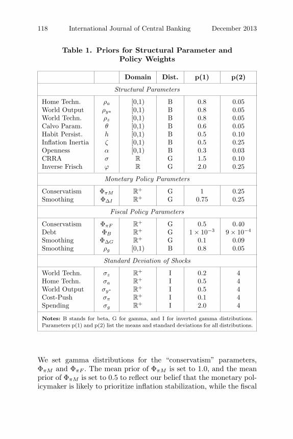
Table 1 summarizes prior distributions for structural parame-ters, policy objectives, and shocks. They are consistent with priorsused in, e.g., Smets and Wouters (2003) and Lubik and Schorfheide(2006). We set relatively wide priors for all parameters which affectpersistence of the propagation mechanism: the price indexationparameter ζ is beta-distributed with mean 0.5 and standard errorof 0.25, and the habit persistence parameter h is beta-distributedwith mean 0.5 and standard error of 0.10. Priors for elasticities σand ϕ are consistent with, e.g., Adjemian, Paries, and Moyen (2008),Justiniano and Preston (2010a), and Liu and Mumtaz (2011).

Parameters ΦπM , ΦΔI , ΦπF , ΦΔG, and ΦB measure the extent ofdeviation of the empirical policy objectives from those microfounded.

14We work with one-period debt stock; its proportion in the total debt stockis relatively small over the observed period.


Table 1. Priors for Structural Parameter andPolicy Weights

Domain Dist. p(1) p(2)

Structural Parameters

Home Techn. ρa [0,1) B 0.8 0.05World Output ρy∗ [0,1) B 0.8 0.05World Techn. ρz [0,1) B 0.8 0.05Calvo Param. θ [0,1) B 0.6 0.05Habit Persist. h [0,1) B 0.5 0.10Inflation Inertia ζ [0,1) B 0.5 0.25Openness α [0,1) B 0.3 0.03CRRA σ R G 1.5 0.10Inverse Frisch ϕ R G 2.0 0.25

Monetary Policy Parameters

Conservatism ΦπM R+ G 1 0.25

Smoothing ΦΔI R+ G 0.75 0.25

Fiscal Policy Parameters

Conservatism ΦπF R+ G 0.5 0.40

Debt ΦB R+ G 1 × 10−3 9 × 10−4

Smoothing ΦΔG R+ G 0.1 0.09

Smoothing ρg [0,1) B 0.8 0.05

Standard Deviation of Shocks

World Techn. σz R+ I 0.2 4

Home Techn. σa R+ I 0.5 4

World Output σy∗ R+ I 0.5 4

Cost-Push σπ R+ I 0.1 4

Spending σg R+ I 2.0 4

Notes: B stands for beta, G for gamma, and I for inverted gamma distributions.Parameters p(1) and p(2) list the means and standard deviations for all distributions.

We set gamma distributions for the “conservatism” parameters,ΦπM and ΦπF . The mean prior of ΦπM is set to 1.0, and the meanprior of ΦπM is set to 0.5 to reflect our belief that the monetary pol-icymaker is likely to prioritize inflation stabilization, while the fiscal


policymaker may consider inflation stabilization less of a priority.However, both prior distributions are very wide and allow bothposterior means to exceed one.

The interest rate smoothing target weight ΦΔI can be interpretedas a measure of importance of this target relative to the inflationstabilization target. It is widely accepted that the monetary author-ities consider the inflation target to be most important, and it mightbe difficult to justify the mean posterior of ΦΔI if it exceeds one.Note, however, that ΦΔI directly affects the instrument inertia inthe implied policy reaction function. The empirical reaction functionmay not be fully determined by either commitment or discretion; itmay have some non-strategic components which we cannot identifywithin this framework. The presence of such non-strategic compo-nents may imply a large estimate of ΦΔI . Following Dennis (2006)and Ilbas (2010), we do not constrain ΦΔI to be less than one. Wechoose gamma distribution with mean 0.75 and standard error of0.25; this gives us a very wide prior.

There is no wide agreement that the policy weight on instru-ment smoothing in fiscal objectives should not dominate the inflationtarget. However, because we remove the stochastic trend from thegovernment share over the observed period, we do not expect to finda great deal of the fiscal instrument smoothing. We do not expect tofind an important debt stabilization target either, given the observedhigh and persistent debt-to-output ratio in the United Kingdom. Toreflect these beliefs, we choose gamma distribution with mean 0.1and standard error of 0.09 for ΦΔG and choose gamma distributionwith mean 1 × 10−3 and standard error of 9 × 10−4 for ΦB.

All shock variances are assumed to be distributed as invertedgamma distribution. Their means are taken from similar studies,predominantly from Dennis (2006), Lubik and Schorfheide (2006),Ilbas (2010), and Givens (2012).

Finally, some priors are more dispersed than others. Note thatmore-diffuse priors do not necessarily deliver higher marginal datadensity. While the in-sample fit improves slightly, wider priors relaxsome of the parameter restrictions, and this leads to a larger penaltyfor model complexity. The second effect can outweigh the firstone, and this leads to an overall fall in the marginal data density.We therefore make a prior more concentrated when such effect isevident.


4. Empirical Results

4.1 Parameter Estimates

Markov chain Monte Carlo methods, described in, e.g., Lubik andSchorfheide (2006), are used to generate draws from the posteriordistribution of model parameters. We present the summary statisticsin tables 2–4.

Overall, the estimates of the structural parameters fall withinplausible ranges, consistent with most of the literature, and aresimilar for commitment and discretion; see table 2.

The estimate of the Calvo parameter θ implies that prices remainfixed between two and three quarters. The price indexation param-eter ζ is estimated rather moderately: when firms adjust the price,less than half of them change prices optimally rather than adopta rule of thumb and index the growth rate of prices to the pastobserved inflation rate. These estimates are consistent with thoseobtained in Lubik and Schorfheide (2006).

We do not find evidence of substantial habit persistence, meas-ured by parameter h; this is similar to findings in Liu and Mumtaz(2011) for the United Kingdom and in Justiniano and Preston(2010b) for New Zealand. The estimate of the preference param-eter α is lower than the UK import share, and this is consistentwith much of the open-economy literature; see, e.g., Lubik andSchorfheide (2007) and Justiniano and Preston (2010a). The inverseof the intertemporal elasticity of substitution, σ, is consistent withthose obtained in the literature, e.g., Justiniano and Preston (2010a,2010b).

These results are interrelated and are the consequence of fittingequation (19) to the data. If we treat the terms of trade as a non-observable variable, then the tension between the prior and posteriorfor α, σ, and h is greatly reduced.

The marginal data density is relatively flat in the inverse elastic-ity of labor supply, φ, as the posterior distribution of φ is not muchdifferent from the prior.

All priors for policy parameters do not conflict with the data;see table 3. The mean posterior of ΦπM is only slightly less thanthe mean prior, and the posterior distribution is only slightly moreconcentrated than the prior distribution. It implies that the weight


Table 2. Estimated Structural Parameters and Shocks

Monetary-Fiscal Model Monetary Model

Discretion Commitment Discretion Commitment

Structural Parameters

Home Techn. ρa 0.83 0.84 0.87 0.87[0.77,0.89] [0.77,0.90] [0.82,0.92] [0.81,0.93]

World Output ρy∗ 0.84 0.83 0.83 0.82[0.79,0.90] [0.78,0.89] [0.77,0.90] [0.75,0.88]

World Techn. ρz 0.87 0.88 0.85 0.85[0.82,0.92] [0.83,0.93] [0.79,0.91] [0.79,0.91]

Calvo Param. θ 0.64 0.62 0.70 0.63[0.58,0.70] [0.54,0.67] [0.64,0.76] [0.57,0.70]

Habit Persist. h 0.09 0.10 0.08 0.08[0.05,0.12] [0.05,0.14] [0.05,0.11] [0.05,0.11]

Inflation Inertia ζ 0.64 0.75 0.79 0.76[0.52,0.77] [0.61,0.88] [0.69,0.90] [0.60,0.91]

Openness α 0.26 0.26 0.27 0.27[0.21,0.30] [0.22,0.31] [0.22,0.32] [0.22,0.32]

CRRA σ 1.23 1.22 1.19 1.19[1.10,1.36] [1.09,1.35] [1.06,1.32] [1.05,1.32]

Inverse Frisch φ 2.03 2.03 1.87 1.92[1.64,2.42] [1.63,2.42] [1.50,2.15] [1.54,2.26]

Standard Deviation of Shocks

World Techn. σz 0.18 0.23 0.25 0.29[0.15,0.22] [0.18,0.28] [0.19,0.30] [0.23,0.36]

Home Techn. σa 0.38 0.41 0.92 0.89[0.32,0.45] [0.34,0.49] [0.75,1.08] [0.73,1.04]

World Output σy∗ 1.15 1.17 1.30 1.30[0.97,1.34] [0.97,1.37] [1.10,1.50] [1.10,1.51]

Cost-Push σπ 0.14 0.14 0.14 0.14[0.12,0.16] [0.12,0.16] [0.12,0.16] [0.12,0.16]

Spending σg 2.25 2.28 2.23 2.24[1.92,2.59] [1.92,2.61] [1.90,2.57] [1.90,2.57]

Notes: Mean and posterior percentiles are from eight chains of 100,000 draws gener-ated using the random-walk Metropolis algorithm, where we discard the initial 50,000draws. Convergence diagnostics were assessed using trace plots.


Table 3. Estimated Structural Parameters and Weights

Monetary-Fiscal Model Monetary Model


Monetary Policy Parameters

Conservatism ΦπM 0.91 0.92 0.78 0.90[0.55,1.27] [0.56,1.25] [0.45,1.11] [0.52,1.26]

Smoothing ΦΔI 0.90 0.80 1.09 0.92[0.49,1.27] [0.43,1.14] [0.64,1.52] [0.53,1.25]

Fiscal Policy Parameters

Conservatism ΦπF 0.39 0.35 — —[0.01,0.79] [0.04,0.66]

Debt ΦB 0.00 0.00 — —[0.00,0.00] [0.00,0.00]

Smoothing ΦΔG 0.01 0.01 — —[0.00,0.03] [0.00,0.03]

Smoothing ρg — — 0.85 0.85[0.80,0.90] [0.80,0.90]

Table 4. Data Density

Type of Type of Hyper-Policy BVAR Data parameterRegime Prior Density λ

Monetary- DSGE Discretion — −226.25 —Fiscal DSGE Commitment — −231.65 —Model BVAR — Discretion −183.37 0.98

[0.70,1.24]BVAR — Commitment −182.20 0.98

[0.72,1.23]Monetary DSGE Discretion — −288.37 —

Model DSGE Commitment — −289.52 —BVAR — Discretion −203.45 0.76

[0.60,0.92]BVAR — Commitment −205.05 0.74

[0.72,1.23]


on inflation stabilization is consistent with the microfounded weightand is relatively large. There is no tension between the prior and pos-terior of ΦΔI : although the mean posterior is slightly higher thanthe mean prior, it remains below one and the confidence interval isnot too wide.

The policy priorities of the fiscal policymaker are described byrelative weights ΦπF , ΦΔG, and ΦB. The posterior of the conser-vatism weight, ΦπF , is more concentrated than the (very wide) prior,with the mean shifted towards zero. This implies that the relativeweight on the inflation target is lower than the microfoundations sug-gest. The fiscal smoothing weight ΦΔG is very small; this is likely tobe a consequence of the chosen detrending method. We did not findany evidence that the fiscal policymakers have the debt target, ΦB.

The estimates of standard errors of structural shocks are in linewith those obtained in most of the literature; see, e.g., Smets andWouters (2003) and Lubik and Schorfheide (2007) for equally styl-ized models. Standard errors of technology and cost-push shocksare relatively low and, similar to results in Lubik and Schorfheide(2007), the standard error of the foreign demand shock is relativelyhigh. The foreign demand shock is likely to accumulate various mis-specifications of our simple model.

4.2 Commitment vs. Discretion

If we allow for policy delegation, then the dynamics of the econ-omy under discretion can be made very similar to the one undercommitment.15 Additionally, if the private sector is predominantlybackward looking, then the difference between the dynamics of theeconomy under commitment and discretion is small. Our model hasboth these features. First, we have estimated some degree of habitpersistence and inflation inertia. Second, we have also estimated dif-ferent parameters of policy objectives of the two policymakers. Itmight become difficult to distinguish between the two policy regimes.

Nevertheless, there are some differences between the estimatedparameters under discretion and commitment. First, to fit the same

15Interest rate smoothing, price-level targeting, and speed-limit policy are alldesigned to approximate the commitment equilibrium in a simple New Keynesianmodel. In models with optimizing fiscal policy, such result may be less clear ifthe policymakers choose to engage in a fight.


data, the price setters under commitment reset prices more fre-quently, but most of these changes are based on the rule of thumbrather than on optimality. The mean share of the rule-of-thumb set-ters under commitment is 10 percent greater than under discretion.Second, the monetary policymaker under discretion has a biggerpenalty on the interest rate smoothing target than the policymakerunder commitment. In this model, given the same policy objectivesand parameters of the model for commitment and discretion, theoptimal policy under commitment generates lower volatility of infla-tion and higher volatility of interest rate. At the same time, inflationis found to be more sensitive to interest rate changes under commit-ment than under discretion. Therefore, in order to fit both models tothe same data on interest rate and inflation, we have to have a lowerweight on interest rate smoothing under commitment. An increasein this weight under commitment generates lower volatility of inter-est rate and much higher volatility of inflation, which is rejected bythe data.

In order to improve our understanding of the dynamics of econ-omy under the two policies, we compute impulse response func-tions. Figure 1 reports the responses of endogenous variables toone-standard-deviation shocks. Each sub-plot plots results for com-mitment and discretion together and shows mean responses ofobservable variables together with 5th and 95th percentiles. We onlyplot the first ten quarters, as all variables converge back to their baselines in the long run.16

A positive home technology shock AH reduces the marginal costand drives inflation down. The monetary policymaker reduces theinterest rate so consumption and output rise. The real exchangerate depreciates. The fiscal policymaker increases spending such thatthe government share rises. Under commitment, the interest rateis reduced by more, which leads to higher consumption, inflationovershooting, and a reduction in government debt.

An increase in the world output ηy∗ increases foreign demandfor both home and foreign goods. This results in an appreciationof the real exchange rate. Because of the risk-sharing assumption,consumers increase consumption of foreign goods, which leads to an

16Because the debt target ΦB �= 0, although very small, the debt under com-mitment is not a unit-root variable.


Figure 1. Impulse Responses to One-Standard-DeviationStructural Shocks

0 5 10-0.015

-0.01

-0.005

0

0.005

0.01

AH

πH

0 5 10-0.08

-0.06

-0.04

-0.02

0i

0 5 100

0.1

0.2

0.3

0.4

Y/AW

0 5 10-0.1

0

0.1

0.2

0.3G/Y

0 5 10-0.06

-0.04

-0.02

0

0.02

0.04

B/AW

0 5 100

0.1

0.2

0.3

0.4

C/AW

0 5 100

0.1

0.2

0.3

0.4

0.5S

0 5 10-0.01

-0.005

0

0.005

0.01

η* y

0 5 10-0.03

-0.02

-0.01

0

0.01

0 5 10-0.1

-0.05

0

0.05

0.1

0 5 10-0.1

0

0.1

0.2

0.3

0 5 100

0.02

0.04

0.06

0.08

0.1

0 5 100

0.1

0.2

0.3

0.4

0.5

0 5 10-2

-1.5

-1

-0.5

0

0 5 10-0.05

0

0.05

0.1

0.15

0.2

ηπ

0 5 10-0.02

0

0.02

0.04

0.06

0.08

0 5 10-0.1

-0.05

0

0.05

0.1

0 5 10-0.05

0

0.05

0.1

0.15

0 5 10-0.05

0

0.05

0.1

0.15

0 5 10-0.15

-0.1

-0.05

0

0.05

0 5 10-0.2

-0.15

-0.1

-0.05

0

0.05

0 5 10-0.04

-0.02

0

0.02

0.04

AW

0 5 100

0.05

0.1

0.15

0.2

0 5 10-0.05

0

0.05

0.1

0.15

0 5 10-0.3

-0.2

-0.1

0

0.1

0.2

0 5 10-0.15

-0.1

-0.05

0

0.05

0 5 10-0.05

0

0.05

0.1

0.15

0 5 10-0.1

0

0.1

0.2

0.3

commitmentconf.int.

commitmentmean

discretionconf.int.

discretionmean


initial reduction in domestic output. Inflation falls and the inter-est rate is reduced. The interest rate under commitment is reducedby more, resulting in inflation overshooting and lower debt. Fiscalpolicy increases spending and the government share.

A positive cost-push shock ηπ increases inflation, and optimalmonetary policy raises the interest rate in response. This leads tolower consumption and output and a consequent reduction in infla-tion. Fiscal policy reduces spending. The real exchange rate appreci-ates. Under commitment, the interest rate is raised by more, whichleads to greater appreciation of the real exchange rate and a greaterfall in consumption. The resulting reduction in marginal cost is insuf-ficiently strong to outweigh the inflation persistence and deliver thesame speed of reduction in inflation as under discretion. The gov-ernment share rises because of the bigger fall in consumption andoutput.

A positive worldwide productivity shock AW results in the realexchange rate depreciation. The productivity-adjusted output rises.The initial impact on habit-adjusted consumption is positive becauseof the increase in real wage following the shock. The higher marginalcost drives inflation up. The optimal interest rate is raised. Govern-ment spending has to be lower to control the accumulation of debt.Interest rate under commitment rises higher than under discretion.This ensures quick reduction in inflation with overshooting.

4.3 Model Fit

Table 4 reports the marginal data density for both policy regimes.This is a measure of relative fit and allows one to compare differentspecifications of the model. A comparison of marginal data densitiesleads to the conclusion that the regime of fiscal leadership in theUnited Kingdom can be best described as discretion. The differencebetween the log-marginal data densities can be interpreted as log-posterior odds under the assumption that the two specifications haveequal prior probabilities. Our finding suggests that the probabilitythat the actual data was generated by a model with optimal com-mitment policy, rather than by a model with optimal discretionarypolicy, is less than 1 percent. In interpretation of Kass and Raftery(1995), there is a “substantial” evidence in favor of discretion overcommitment.


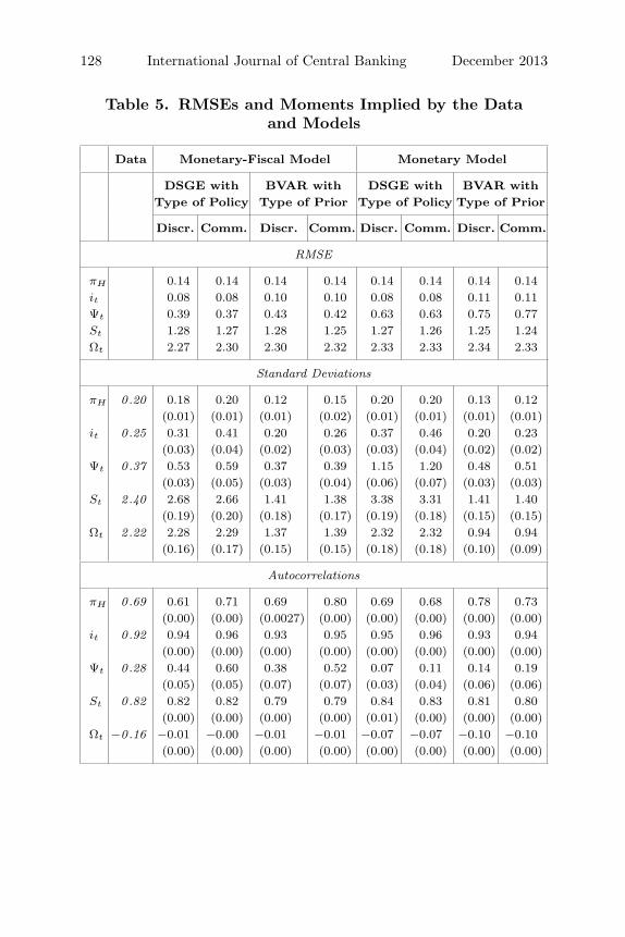
While the data density provides a measure of relative fit, wealso present root mean squared errors (RMSEs) and second-ordermoments which measure absolute fit; see, e.g., Justiniano andPreston (2010b) and Rabanal and Tuesta (2010). Table 5 reportsRMSEs and second-order moments for the data and the correspond-ing statistics implied by the estimated models. We report meanswith standard errors in parentheses.

The DSGE model under discretion produces good fit of stan-dard deviations of all variables—in particular, of interest rate andinflation. The volatility of the output growth rate Ψt is slightly over-estimated under both discretion and commitment. The volatilityof interest rate is substantially overestimated under commitment.Namely, these properties produce most of the differences in impulseresponses between the two models in figure 1.

Empirical autocorrelation of inflation is best captured by thecommitment model, while the discretion model underestimates it.Both models overestimate the autocorrelation of the growth rateof output and underestimate the autocorrelation of the governmentshare. The autocorrelation of the terms of trade is captured reason-ably well.

Further, table 6 reports autocorrelations up to the fifth order.The autocorrelations generated by the model of discretion are closeto the data autocorrelations for all variables. However, both discre-tion and commitment models are able to match empirical autocor-relations closely.

To assess the degree of model fit, we also report marginal datadensities for reduced-form vector autoregressions with four lags, esti-mated under different Minnesota-type priors. More specifically, fol-lowing Del Negro and Schorpfheide (2004), Lubik and Schorfheide(2006), and Adjemian, Paries, and Moyen (2008), we populate theoriginal data sample with additional artificial data generated by theDSGE model. The relative importance of the prior information canbe measured by parameter λ = N/T, where N is the size of theartificial sample and T is the size of the data sample. We estimatethe optimal weight, λ, of either commitment or discretion DSGEprior in the BVAR model. Following Del Negro and Schorpfheide(2004), we call it the DSGE-VAR or BVAR model interchangeably.The relative importance of the prior information is a measure of thedegree of misspecification of the model. If λ is estimated to be high,


Table 5. RMSEs and Moments Implied by the Dataand Models

Data Monetary-Fiscal Model Monetary Model

DSGE with BVAR with DSGE with BVAR withType of Policy Type of Prior Type of Policy Type of Prior

Discr. Comm. Discr. Comm. Discr. Comm. Discr. Comm.

RMSE

πH 0.14 0.14 0.14 0.14 0.14 0.14 0.14 0.14it 0.08 0.08 0.10 0.10 0.08 0.08 0.11 0.11Ψt 0.39 0.37 0.43 0.42 0.63 0.63 0.75 0.77St 1.28 1.27 1.28 1.25 1.27 1.26 1.25 1.24Ωt 2.27 2.30 2.30 2.32 2.33 2.33 2.34 2.33

Standard Deviations

πH 0 .20 0.18 0.20 0.12 0.15 0.20 0.20 0.13 0.12(0.01) (0.01) (0.01) (0.02) (0.01) (0.01) (0.01) (0.01)

it 0 .25 0.31 0.41 0.20 0.26 0.37 0.46 0.20 0.23(0.03) (0.04) (0.02) (0.03) (0.03) (0.04) (0.02) (0.02)

Ψt 0 .37 0.53 0.59 0.37 0.39 1.15 1.20 0.48 0.51(0.03) (0.05) (0.03) (0.04) (0.06) (0.07) (0.03) (0.03)

St 2 .40 2.68 2.66 1.41 1.38 3.38 3.31 1.41 1.40(0.19) (0.20) (0.18) (0.17) (0.19) (0.18) (0.15) (0.15)

Ωt 2 .22 2.28 2.29 1.37 1.39 2.32 2.32 0.94 0.94(0.16) (0.17) (0.15) (0.15) (0.18) (0.18) (0.10) (0.09)

Autocorrelations

πH 0 .69 0.61 0.71 0.69 0.80 0.69 0.68 0.78 0.73(0.00) (0.00) (0.0027) (0.00) (0.00) (0.00) (0.00) (0.00)

it 0 .92 0.94 0.96 0.93 0.95 0.95 0.96 0.93 0.94(0.00) (0.00) (0.00) (0.00) (0.00) (0.00) (0.00) (0.00)

Ψt 0 .28 0.44 0.60 0.38 0.52 0.07 0.11 0.14 0.19(0.05) (0.05) (0.07) (0.07) (0.03) (0.04) (0.06) (0.06)

St 0 .82 0.82 0.82 0.79 0.79 0.84 0.83 0.81 0.80(0.00) (0.00) (0.00) (0.00) (0.01) (0.00) (0.00) (0.00)

Ωt −0 .16 −0.01 −0.00 −0.01 −0.01 −0.07 −0.07 −0.10 −0.10(0.00) (0.00) (0.00) (0.00) (0.00) (0.00) (0.00) (0.00)


Table 6. Autocorrelations Implied by the Data andModels

Lag Data DSGE BVAR

Type of Policy Type of Prior


Inflation, πH

1 0.69 0.61 0.71 0.69 0.80(0.00) (0.00) (0.00) (0.00)

2 0.23 0.42 0.41 0.57 0.50(0.00) (0.00) (0.00) (0.00)

3 0.01 0.21 0.22 0.40 0.33(0.00) (0.00) (0.00) (0.00)

4 0.03 0.05 0.11 0.25 0.21(0.00) (0.00) (0.00) (0.00)

5 0.07 −0.06 0.06 0.14 0.14(0.00) (0.00) (0.00) (0.00)

Output Growth Rate, Ψt

1 0.28 0.44 0.60 0.38 0.52(0.05) (0.05) (0.07) (0.07)

2 0.08 0.06 0.10 0.10 0.14(0.02) (0.03) (0.03) (0.04)

3 0.09 0.06 0.10 0.10 0.13(0.02) (0.03) (0.03) (0.04)

4 0.04 0.06 0.09 0.09 0.12(0.02) (0.03) (0.03) (0.04)

5 −0.01 0.05 0.09 0.08 0.11(0.02) (0.03) (0.03) (0.03)

Interest Rate, it

1 0.92 0.94 0.96 0.93 0.95(0.00) (0.00) (0.00) (0.00)

2 0.80 0.85 0.86 0.81 0.82(0.00) (0.00) (0.00) (0.00)

3 0.64 0.74 0.74 0.68 0.67(0.00) (0.00) (0.01) (0.01)

4 0.51 0.63 0.62 0.55 0.52(0.00) (0.00) (0.01) (0.01)

5 0.42 0.53 0.52 0.43 0.41(0.00) (0.00) (0.01) (0.01)

(continued)


Table 6. (Continued)

Lag Data DSGE BVAR

Type of Policy Type of Prior


Terms of Trade, St

1 0.08 0.82 0.82 0.79 0.79(0.00) (0.00) (0.00) (0.00)

2 0.76 0.71 0.70 0.68 0.67(0.01) (0.01) (0.00) (0.00)

3 0.64 0.61 0.59 0.58 0.56(0.00) (0.01) (0.00) (0.00)

4 0.57 0.52 0.49 0.48 0.46(0.01) (0.01) (0.00) (0.01)

5 0.53 0.44 0.42 0.41 0.39(0.01) (0.01) (0.00) (0.01)

Growth Rate of Government Share, Ωt

1 −0.16 −0.01 −0.00 −0.01 −0.01(0.00) (0.00) (0.00) (0.00)

2 −0.00 −0.06 −0.06 −0.08 −0.08(0.00) (0.00) (0.00) (0.00)

3 −0.02 −0.06 −0.05 −0.06 −0.06(0.00) (0.00) (0.00) (0.00)

4 0.42 −0.05 −0.04 −0.05 −0.05(0.00) (0.00) (0.00) (0.00)

5 −0.06 −0.04 −0.04 −0.04 −0.04(0.00) (0.00) (0.00) (0.00)

then it means that the DSGE model imposes useful restrictions toimprove the (in-sample) predictive properties of the BVAR model.Conversely, if λ is estimated to be low, then the DSGE model is notcoherent with the data. Finding λ � 1.0 suggests that the DSGEmodels do impose some useful restrictions: Del Negro et al. (2007)and Adjemian, Paries, and Moyen (2008) demonstrate that λ = 0.35is close to the point where the DSGE provides no useful information,


while λ > 0.6 demonstrates some coherence of the DSGE model withthe data.

Notably, the marginal data densities for both BVARs are almostidentical; see table 4. Both commitment and discretion DSGE mod-els impose similarly useful restrictions. A comparison of DSGE andBVARs can help us to identify the tightest restrictions imposed bythe DSGE models. Table 5 demonstrates that both BVARs improvethe fit of the growth rate of output and interest rate but at theexpense of the fit of other variables. Figure 2 compares impulseresponses of DSGE and DSGE-VAR models under discretion. It isapparent that the dynamics of inflation, interest rate, and the termsof trade is less volatile as implied by the BVAR, but at the sametime we do not observe any big differences in direction of responsesand in their persistence which is implied by this correction.

Finally, figure 3 reports the historic and the one-step-ahead pre-dicted data under the two policy regimes. Both policy regimes resultin very similar estimates.

4.4 Role of Fiscal Policy

We have estimated fiscal policy to be relatively inactive: althoughthere is a general consistency of the data with microfounded pol-icy objectives, fiscal policy does very little to stabilize the economy.Under our assumption of fiscal intraperiod leadership, this is theoptimal outcome, as the fiscal policymaker leaves the stabilizationwork to the monetary policymaker. The monetary policymaker, how-ever, observes fiscal variables and takes them into account whenformulating policy. In this section we argue that the state of fiscalstance does play a role in identification of the model.

The evolution of the government debt and fiscal spending areamong the identifying restrictions for the model. To assess theimportance of these restrictions, we reestimate the model exclud-ing the government solvency constraint and treating the governmentshare as following an AR(1) process with coefficient ρg. The mone-tary policymaker is assumed to act either under discretion or com-mitment. The results of estimation are given in table 2, in the lasttwo columns.

Some of the key structural parameters appear to be differentwhen the fiscal problem is excluded. In particular, the Calvo reset


Figure 2. Impulse Responses under Discretion

0 5 10-15

-10

-5

0

5x 10-3

AH

πH

0 5 10-0.06

-0.05

-0.04

-0.03

-0.02

-0.01

0i

0 5 10-0.1

0

0.1

0.2

0.3

0.4

Δ(Y/AW

)

0 5 10-0.2

-0.1

0

0.1

0.2Δ(G/Y)

0 5 100

0.1

0.2

0.3

0.4

0.5S

0 5 10-6

-4

-2

0

2x 10-3

η y*

0 5 10-0.02

-0.015

-0.01

-0.005

0

0 5 10-0.1

-0.05

0

0.05

0.1

0 5 10-0.2

-0.1

0

0.1

0.2

0.3

0 5 10-2

-1.5

-1

-0.5

0

0 5 10-0.05

0

0.05

0.1

0.15

0.2

ηπ

0 5 10-0.02

0

0.02

0.04

0.06

0 5 10-0.08

-0.06

-0.04

-0.02

0

0.02

0 5 10-0.05

0

0.05

0.1

0.15

0 5 10-0.15

-0.1

-0.05

0

0.05

0 5 10-0.01

0

0.01

0.02

0.03

AW

0 5 100

0.05

0.1

0.15

0.2

0 5 100

0.1

0.2

0.3

0.4

0 5 10-0.3

-0.2

-0.1

0

0.1

0.2

0 5 10-0.05

0

0.05

0.1

0.15

0.2

DSGEconf.int.

DSGEmean

DSGE-VARconf.int.

DSGE-VARmean


Figure 3. The Data and One-Step-Ahead Forecast

1994 1996 1998 2000 2002 2004 2006 20080

1

2

3

4

5

πH

1994 1996 1998 2000 2002 2004 2006 20080

1

2

3

4

5

6

7

8

i

1994 1996 1998 2000 2002 2004 2006 2008-0.5

0

0.5

1

1.5

2Ψ

Data DiscretionDSGE

CommitmentDSGE

DiscretionDSGE-VAR

CommitmentDSGE-VAR

1994 1996 1998 2000 2002 2004 2006 2008-4

-2

0

2

4

6

8S

probability, the degree of inflation inertia, and volatility of hometechnology shocks are larger when the fiscal block is ignored; thedifference is particularly large for the preferred specification of theoptimal discretion. The monetary policy parameters are affected tooonce the fiscal block becomes exogenous: the monetary policymakeris less inflation conservative and operates with greater interest ratesmoothing. All these changes in estimated parameters are requiredto generate greater endogenous persistence observed in the data.

Table 4 demonstrates that the monetary model leads to lowermarginal data density. (There is also much less difference betweencommitment and discretion.) The absolute fit is assessed in table 5.Standard deviations of interest rate, terms of trade, and the growthrate of output are substantially overestimated. The autocorrelationof the growth rate of output is underestimated and there is a bigincrease in RMSE for this variable. At the same time, the autocor-relation of the government share is much less underestimated.


To understand these results, we look at the role of the governmentdebt accumulation equation in the model.

First, the debt accumulation process is highly persistent underboth commitment and discretion. Its persistence propagates throughthe whole system; in particular, in the case of discretion where allreaction functions are time invariant and can be written as linearfunctions of predetermined states, the speed of convergence of allvariables, including debt, is the same. If we remove the governmentbudget constraint from the system, then in order to fit the same per-sistent data, we require more inflation inertia and a higher penaltyon policy instrument movements. This role of debt process as per-sistent process might be played by some other “slow” processes, likethe capital accumulation process, which are omitted from our simplemodel.

Second, the debt accumulation process is potentially explosive.All economic agents are aware of this and should make decisions thatare compatible with non-explosiveness of debt dynamics. In particu-lar, the fiscal policymaker may optimally prefer to feed back on debtstrong enough in order to allow the monetary policymaker to concen-trate on inflation stabilization tasks. The monetary-fiscal model esti-mation results are consistent with non-explosiveness of debt. Oncethe government budget constraint is removed and the dynamics offiscal instrument is approximated by an AR(1) exogenous process,the monetary policymaker does not take into account whether theproblem of debt stabilization is resolved or not. This yields highervolatility of interest rate to fit the volatility of inflation in the data.Higher penalty on the instrument smoothing terms would result inhigher volatility of inflation, inconsistent with the data. This roleof the debt accumulation process as a potentially explosive processmay not be played by an intrinsically stable process like the capitalaccumulation process.

One can argue that the monetary policymaker alone can pre-commit to the chosen plan, while if we estimate monetary and fiscalinteractions jointly, then discretionary policy of fiscal policymakersresults in the overall dominance of discretion. Indeed, we find thatthe gap between discretion and comment reduced once we excludedthe fiscal sector from the economy. However, the smaller differencecan also be a result of higher estimated persistence of the economyand the smaller role of expectations.


Finally, results from corresponding DSGE-VAR models suggestthat there is a reduction in λ, so the monetary DSGE model imposestighter restrictions on the data. The BVAR marginal data densityvalues improve by about eighty units and are closer to those obtainedin more general monetary-fiscal DSGE-VAR models. Also, the first-and second-order moments are not as closely matched as in themonetary-fiscal model.

5. Conclusions

This paper identifies the degree of precommitment in monetary andfiscal policy interactions in the United Kingdom. We specify a small-scale structural general equilibrium model of a small open economyand estimate it using Bayesian methods. Unlike most of the exist-ing empirical research, we explicitly take into account the solvencyconstraint faced by the fiscal authorities. We also assume that theauthorities act non-cooperatively and may have different objectives.

We find that the model of discretionary policy explains the databetter than the model of commitment policy. We find that bothpolicymakers put smaller weight on inflation stabilization than issocially optimal. The fiscal policymaker pays much less attention toinflation stabilization than the monetary policymaker. The presenceof fiscal block in the model plays the important role in identificationof monetary policy and structural parameters.

Appendix 1. Social Welfare

Social welfare is written as

W =∞∑

t=0

βt

(x1−σ

t

1 − σ+ χ

g1−σt

1 − σ− N1+ϕ

t

1 + ϕ

).

Linearization yields

W =∞∑

t=0

βt

(x1−σ

(xt +

12(1 − σ)x2

t

)+ χg1−σ

(gt +

12(1 − σ)g2

t

)

−N1+ϕ

(Nt +

12(1 + ϕ)N2

t

))+ tip(3),


where tip(3) includes terms independent of policy of the third orderand higher. Production function (14) yields the exact relationshipNt = Δt + yt − AHt. We substitute Nt out and use

∞∑t=0

βtΔt =θ

1 − θβΔ−1 +

12

∞∑t=0

βt εθ (1 − ζ)λ

×(

π2Ht +

ζ

θ (1 − ζ)(πHt − πHt−1)

2)

to yield

W =∞∑

t=0

βt

(x1−σ

(xt +

12(1 − σ)x2

t

)+ χg1−σ

(gt +

12(1 − σ)g2

t

)

−χNN1+ϕ(yt + 1

2εθ(1−ζ)

λ

(π2

Ht + ζθ(1−ζ) (πHt − πHt−1)

2)

+ 12(1 + ϕ)N2

t

)⎞⎠

+ tip(3).

The linearized-up-to-second-order national income identity andthe international risk-sharing condition yield

yt +12y2

t = (1 − α)c

y

(ct + αηSt +

12αη (−η + 2αη + 1 − α) S2

t

+12c2t + αηStct

)+

g

y

(gt +

12g2

t

)

+ αc

y

(ηSt + c∗

t +12η2S2

t +12c∗2t + ηStc

∗t

)

σxt +12σ2x2

t = (1 − α)St + σx∗t +

12

(ηα − 2α + 1)(1 − α)

(1 − α)2S2t

+12σ2x∗2

t + σ(1 − α)Stx∗t .

Combining them allows us to substitute out the terms of trade:

yt =c

y(1 − α)ct +

g

ygt +

c

y

αη (2 − α) σ

(1 − α)xt +

c

y

12

αη (2 − α) σ2

(1 − α)x2

t

+c

y

12αη

(α (η − αη + 1) − (1 − α)2

) σ2

(1 − α)2(xt − x∗

t )2


− c

y

αη (2 − α) σ2

(1 − α)(xt − x∗

t ) x∗t + (1 − α)

c

y

αησ

(1 − α)(xt − x∗

t ) ct

+c

y

αησ

(1 − α)(xt − x∗

t ) c∗t +

g

y

12g2

t − 12y2

t + (1 − α)c

y

12c2t .

Using

∞∑t=0

βtxt = − h

(1 − h)c−1 +

(1 − βh)(1 − h)

∞∑t=0

βtct,

we arrive at

W =∞∑

t=0

βtWt,

where

Wt =(

− x1−σ

N1+ϕ

(1 − βh)(1 − h)

+αη (2 − α) σ (1 − βh)

(1 − α) (1 − h)c

y+ (1 − α)

c

y

)ct

+(

g

y− χg1−σ

N1+ϕ

)gt +

12

(c

y

αη (2 − α) σ2

(1 − α)− x1−σ

N1+ϕ(1 − σ)

)x2

t

+12

εθ (1 − ζ)λ

(π2

Ht +ζ

θ(1 − ζ)(πHt − πHt−1)

2)

+c

y

12

(α (η − αη + 1) − (1 − α)2)αησ2

(1 − α)2(xt − x∗

t )2

+c

yαησ (xt − x∗

t ) ct − c

y

(2 − α) αησ2

(1 − α)(xt − x∗

t ) x∗t

+c

y

αησ

(1 − α)(xt − x∗

t ) c∗t +

12(1 + ϕ)(yt − AHt)2

+12(1 − α)

c

yc2t +

12

(g

y− χg1−σ

N1+ϕ(1 − σ)

)g2

t − 12y2

t + tip(3).

We are interested in comparing stabilization performance of differentpolicies; therefore, we assume that a time-invariant labor subsidy off-sets monopolistic distortions, x1−σ

N1+ϕ = cy (σαη(2−α)

(1−α) + (1−h)(1−α)(1−βh) ). We


chose χ so that gy = χ g1−σ

N1+ϕ . This yields the quadratic approximationto the social welfare loss in the form

Wt = π2Ht +

ζ

γ (1 − ζ)(πHt − πHt−1)

2 +λσ (1 − θ)εγ (1 − ζ)

g2t

+λϕ

εγ (1 − ζ)

(y2

t − (1 + ϕ)ϕ

AHt

)2

+2θλ

εγ (1 − ζ)

(12Ψxx2

t + (1 − α)c2t −

αησ2(αη − α2η + 1

)(1 − α)2

xtx∗t

+ αησxtct +ηασ

(1 − α)xtc

∗t − αησx∗

t ct

)+ tip(3),

where Ψx = σαη(1−α)((2−α)(2σ−1)+ ((1−α)η+1)ασ

(1−α) )− (1−h)(1−α)(1−σ)(1−βh) −

αησ2.

Appendix 2. Theoretical Framework

Our model belongs to the class of non-singular linear stochasticrational expectations models of the type described by Blanchardand Kahn (1980), augmented by a vector of control instruments.

We label the two policymakers as leader (L) and follower (F ),and denote them with index i, i ∈ {L, F}. (In this paper the leader isthe fiscal policymaker and the follower is the monetary policymaker.)

The evolution of the economy is explained by the followingsystem: [

yt+1Etxt+1

]=

[A11 A12A21 A22

] [yt

xt

]

+[

B11 B12B21 B22

] [uL

t

uFt

]+

[εt+10

], (30)

where yt is a vector of predetermined variables with initial conditionsy0 given, yt = [at, y

∗t , επ

t , bt]′, xt is a vector of non-predetermined (or

jump) variables, and xt = [πHt, xt]′ where xt ≡ yt − gt. uF

t and uLt

are the two vectors of policy instruments of the two policymakers,named F and L. uF

t = it and uLt = gt in the model. εt is a vector of

i.i.d. shocks.


Each of the two policymakers has the following loss functions:

Jjt =

12Et

∞∑s=t

βs−t(G′sQjGs), (31)

where j = {L, F} and Gjs is a vector of goal variables of policy-

maker i, which is a linear function of state variables and instruments,Gj

s = Cj[y′s, x

′s, u

L′s , uF ′

s

]′.Commitment policy means that each policymaker is able to com-

mit, with full credibility, to a policy plan (Currie and Levine 1993).Thus, the policy plan has to specify the desired levels of the tar-get variables (e.g., inflation, the output gap, etc.) at all current andfuture dates and states of nature.

Assumption 1. At each time t the follower observes the currentdecision of the leader uL

t . The private sector observes both decisionsuL

t and uFt .

Assumption 2. At any time t both policymakers know assumption 1.

The follower observes policy of the leader and reacts to it. Theleader knows the follower reacts to its policy and is able to exploitit.

Assumption 3. Suppose at time t the private sector and the policy-makers only responds to the current state⎡

⎣ xt

uLt

uFt

⎤⎦ = −

⎡⎣ Nd

FL1

FF2

⎤⎦ yt. (32)

Assumption 4. At each time t, the private sector observes the cur-rent policy decisions uL

t , uFt and expects that future policymakers will

reoptimize, and will apply the same decision process and implementdecision [FL′

1 , FF ′2 ]′. At each time t the follower observes the current

policy decision of the leader uLt and expects that future leaders will

reoptimize, and will apply the same decision process and implementdecision FL

1 .


Problem 1 (Leadership under Commitment). Under commitmentpolicy the follower solves

min{uF

s }∞s=t

12Et

∞∑s=t

βs−t(GF ′s QF GF

s ) (33)

subject to constraint (30).The leader solves

min{uL

t }∞s=t

12Et

∞∑s=t

βs−t(GL′s QLGL

s ) (34)

subject to constraint (30) and to the system of first-order conditionsof the follower’s optimization problem.

Policy determined by [FL′1 , FF ′

2 ]′ is commitment policy if both pol-icymakers find it optimal to follow [FL′

1 , FF ′2 ]′ each time s > t, given

assumptions 1–2.

Discretionary policy means that the policymaker treats its opti-mal policy problem, as described above, as one of “sequential opti-mization,” i.e., without committing to any future course of action,it makes the decision that is optimal within that period only.

Problem 2 (Leadership under Discretion). Under discretion thefollower solves

minuF

t

12Et

∞∑s=t

βs−t(GF ′s QF GF

s ) (35)

subject to constraint (30).The leader solves

minuL

t

12Et

∞∑s=t

βs−t(GL′s QLGL

s ) (36)

subject to constraint (30) and to the system of first-order conditionsof the follower’s optimization problem.

Policy determined by [FL′1 , FF ′

2 ]′ is discretionary if both policy-makers find it optimal to follow [FL′

1 , FF ′2 ]′ each time s > t, given

assumptions 1–4.

Finally, we prove the following proposition.


Proposition 1 (First-Order Conditions). A solution to both com-mitment and discretionary leadership problems can be written in thefollowing dynamic form:

zt+1 = Mzt, (37)

vt = −Nzt, (38)

where variable zt ≡ yt under discretion and zt ≡ [y′t, λ

′t]

′ undercommitment and λt are predetermined Lagrange multipliers; vari-able vt = [x′

t, uL′t , uF ′

t ]′. Matrices M and N are functions of policyobjectives QL and QF and of the system matrices A and B.

Proof. We first solve the problem under commitment. The mini-mization problem of the follower can be presented by the followingintraperiod Lagrangian:

HFs =

12βs−t(x′

sQF22xs + 2y′

sQF12xs + y′

sQF11ys + 2uL

s PF ′11 ys + 2uL

s PF ′21 xs

+ 2uF PF ′12 ys + 2uF

s PF ′22 xs + uL

s RF11U

Ls + 2uL

s RF12u

Fs + uF

s RF22v

Fs

+ λFy′s+1(A11ys + A12xs + D1uL

s + B1uFs − ys+1)

+ λFx′s+1(A21ys + A22xs + D2uL

s + B2uFs − xs+1)),

where Lagrange multipliers λFy are non-predetermined (as thoseon predetermined variables) with terminal conditions and λFx arepredetermined with initial conditions. The first-order conditions are

0 = QF22xs + QF

21ys + PF21u

Ls + PF

22uFs + βA′

12λFys+1 + βA′

22λFxs+1 − λFx

s

0 = QF12xs + QF

11ys + PF11u

Ls + PF

12uFs + βA′

11λFys+1 + βA′

21λFxs+1 − λFy

s

0 = PF ′12 ys + PF ′

22 xs + RF ′12uL

s + RF22u

Fs + βB′

1λFys+1 + βB′

2λFxs+1.

The minimization problem of the leader or fiscal policymaker,

HLs =

12βs−t

(x′sQ

L22xs + 2Y ′

sQL12xs + y′

sQL11ys + 2uLPL′

11 ys

+ 2uLPL′21 xs + 2uF PL′

12 ys + 2uFs PL′

22 xs + uLs RL

11uLs + 2uL

s RL12u

Fs

+ uFs RL

22uFs + λLy′

s+1(A11ys + A12xs + D1uLs + B1uF

s − ys+1)


+ νLx′s (βA′

12λFys+1 + βA′

22λFxs+1 − λFx

s + QF22xs + QF

21ys

+ PF21u

Ls + PF

22uFs

)+ λLx′

s+1(A21ys + A22xs + D2uLs + B2uF

s − xs+1)

+ νLy′s

(A′

11βλFys+1 + A′

21βλFxs+1 − λFy

s + QF12xs + QF

11ys

+ PF11u

Ls + PF

12uFs

)+ νLu′

s (PL′12 ys + PL′

22 xs + RF ′12uL

s + RF22u

Fs + βB′

1λFys+1

+ βB′2λ

Fxs+1)),

where Lagrange multipliers λLy are non-predetermined (as thoseon predetermined variables) with terminal conditions and λLx arepredetermined with initial conditions. The first-order conditions are

0 = QL22xs + QL

21ys + PL21u

Ls + PL

22uFs + QF ′

12νLys + QF ′

22νLxs + PF

22νLu′s

+ βA′12λ

Lys+1 + βA′

22λLxs+1 − λLx

s ,

0 = QL12xs + QL

11ys + PL11u

Ls + PL

12uFs + QF ′

11νLys + QF ′

21νLxs + PF

12νLus

+ βA′11λ

Lys+1 + βA′

21λLxs+1 − λLy

s ,

0 = PL′11 ys + PL′

21 xs + RL11u

Ls + RL

12uFs + PF ′

11 νLys + PF ′

21 νLxs + RF

12νLus

+ βD′1λ

Lys+1 + βD′

2λLxs+1,

0 = PL′12 ys + PL′

22 xs + RL′12u

Ls + RL

22uFs + PF ′

12 νLys + PF ′

22 νLxs + RF ′

22νLus

+ βB′1λ

Lys+1 + βB′

2λLxs+1,

0 = A11νLys − νLy

s+1 + A12νLxs + B1ν

Lus ,

0 = A21νLys + A22ν

Lxs − νLx

s+1 + B2νLus ,

0 = A11ys + A12xs + D1uLs + B1uF

s − ys+1,

0 = A21ys + A22xs + D2uLs + B2uF

s − xs+1.

The system of first-order conditions to both optimization prob-lems can be written as

G

[Ks+1Ls+1

]= D

[Ks

Ls

],


where Ks = (y′s, μ

x′s )′ is a predetermined variable and Ls =

(u′s, x

′s, μ

y′s )′ is a non-predetermined variable, and μy′

s and μx′s col-

lect corresponding Lagrange multipliers. Matrix G can be singular,so using singular form decomposition (see Soderlind 1999), we findthe solution of the system in the form

[Ys+1μx

s+1

]= Z11S

−111 T11Z

−111

[Ys

μxs

],

⎡⎣ us

Xs

μys

⎤⎦ = Z21Z

−111

[Ys

μxs

],

(39)

where matrices Z, S, and T are obtained when solving the general-ized eigenvalue problem. Note that S11 and Z11 have to be invertible,but T11 does not need to be. Moreover, if D has any zero roots, thenany transformations with Hermitian matrices leave them zero, andthey are collected in the top left part of T , such that Tii/Sii < 1.

Denote M = Z11S−111 T11Z

−111 , N = −Z21Z

−111 , and matrix N con-

tains first kF + kF + n2 rows of matrix N. Then, system (39) iswritten in the form of (37)–(38).

We now prove the proposition for discretion.Solution to a discretionary problem in any time t gives a value

function for each policymaker i, i ∈ {L, F}, which is quadratic inthe state variables,

W it =

12y′tS

iyt, (40)

a linear relation between the forward-looking variables

xt = −Nyt, (41)

and a linear policy reaction function

uFt = −FF yt − LuL

t , (42)

uLt = −FLyt, (43)

where L = −∂uFt /∂uL

t : in a leadership equilibrium the follower treatsthe leader’s policy instrument parametrically.

We seek solution in the class of matrices with time-invariant coef-ficients. Given y0 and system matrices A and B, matrices N, FF , FL,and L define the trajectories {ys, xs, us}∞

s=t in a unique way andvice versa: if we know that {ys, xs, us}∞

s=t solve the discretionary


optimization problem, then, by construction, there are uniquetime-invariant linear relationships between them which we labelN, FF , FL, and L. Matrix Si defines the cost to go for a policy-maker i along a trajectory. Given the one-to-one mapping betweenequilibrium trajectories and {ys, xs, us}∞

s=t and the sextuple of matri-ces T = {N, FF , FL, L, SF , SL}, it is convenient to continue withdefinition of policy equilibrium in terms of T , not trajectories. Thisapproach has become standard since Oudiz and Sachs (1985) andBackus and Driffill (1986).

The first-order conditions on T are derived in Blake andKirsanova (2011). We substitute (43) into (42) and obtain equation(38) with N = [N ′, (FF −LFL)′, FL′]′. We substitute (41), (42), and(43) into system (30) and obtain the dynamic system, in which firstn1 equations are written in the form of matrix equation (37) withM = A11 − A12N − B11F

L − B12(FF − LFL).

Appendix 3. System Matrices

System (17)–(27) can be brought to the form

πHt = βθ

ΦEtπHt+1 +

ζ

ΦπHt−1 +

λ

Φ

(πcct − πc1ct−1 + πgg

yt + πc∗ c∗

t

+ πc1∗ c∗t−1 +

σh

(1 − h)zt − (ϕ + 1) aHt

)

ct =1

(1 + h)Etct+1 +

h

(1 + h)ct−1 − σc (rt − EtπHt+1) + cc∗ c∗

t

− hα

(1 + h)c∗t−1 − cz zt

bt+1 =1β

(bt − b

yπHt + bgg

yt + bcct − bc1ct−1 + bc∗ c∗

t + bc1∗ c∗t−1

)

+b

yrt − b

yρz zt

yt = ycct − yc1ct−1 + yc∗ c∗t + yc1∗ c∗

t−1 +g

cgy

t ,

where

πc =σ

(1 − h) (1 − α)

(1 + ϕ

(1 − h)σα

), πc1 =

σh (1 + (2 − α) αηϕ)(1 − h) (1 − α)


πg = ϕg

c, πc∗ =

(ϕ

(1 − (2 − α) ησ

(1 − h) (1 − α)

)− σ

(1 − h) (1 − α)

)α

πc1∗ =ασh (1 + (2 − α) ηϕ)

(1 − h) (1 − α), bg = (1 − τ)

g

c, bc =

(gy − τ)σ

(1 − α)σα

bc1 =(

g

y− τ

)(2 − α) αησ

(1 − h) (1 − α)h,

bc∗ =(

g

y− τ

)α

(1 − (2 − α) ησ

(1 − h) (1 − α)

)

bc1∗ =(

g

y− τ

)α (2 − α) ησ

(1 − h) (1 − α)h, σα =

σ

(1 − α + αω)

ω =(2 − α) ση

(1 − h)− (1 − α) , σc =

(1 − h) (1 − α)(1 + h) σ

,

cc∗ =(

1 − ρc∗

(1 + h)

)α, cz = (1 − ρz)

(1 − α)(1 + h)

h,

yc =α (2 − α) ησ

(1 − h) (1 − α)+ (1 − α), yc1 =

α (2 − α) ησh

(1 − h) (1 − α),

yc∗ = α − α (2 − α) ησ

(1 − h) (1 − α), yc1∗ =

α (2 − α) ησh

(1 − h) (1 − α).

Therefore, system (30) can be written in the following matrixform:

⎡⎢⎢⎢⎢⎢⎢⎢⎢⎢⎢⎢⎢⎢⎢⎢⎢⎣

1 0 0 0 0 0 0 0 0 0 00 1 0 0 0 0 0 0 0 0 00 0 1 0 0 0 0 0 0 0 00 0 0 1 0 0 0 0 0 0 00 0 0 0 1 0 0 0 0 0 00 0 0 0 0 1 0 0 0 0 00 0 0 0 0 0 1 0 0 0 00 0 0 0 0 0 0 1 0 0 00 0 0 0 0 0 0 0 1 0 00 0 0 0 0 0 0 0 0 β θ

Φ 00 0 0 0 0 0 0 0 0 σc

1(1+h)

⎤⎥⎥⎥⎥⎥⎥⎥⎥⎥⎥⎥⎥⎥⎥⎥⎥⎦

⎡⎢⎢⎢⎢⎢⎢⎢⎢⎢⎢⎢⎢⎢⎢⎢⎢⎣

zt+1aHt+1c∗t+1c∗t

rt

gH,t

bt+1πHt

ct

EtπHt+1Etct+1

⎤⎥⎥⎥⎥⎥⎥⎥⎥⎥⎥⎥⎥⎥⎥⎥⎥⎦


=

⎡⎢⎢⎢⎢⎢⎢⎢⎢⎢⎢⎢⎢⎢⎢⎢⎢⎢⎣

ρz 0 0 0 0 0 0 0 0 0 00 ρa 0 0 0 0 0 0 0 0 00 0 ρc∗ 0 0 0 0 0 0 0 00 0 1 0 0 0 0 0 0 0 00 0 0 0 0 0 0 0 0 0 00 0 0 0 0 0 0 0 0 0 0

− bρz

y 0 bc∗β

bc1∗β 0 0 1

β 0 − bc1β − b

βybc

β

0 0 0 0 0 0 0 0 0 1 00 0 0 0 0 0 0 0 0 0 1

− λσhΦ(1−h)

λ(ϕ+1)Φ −λπc∗

Φ −λπc1∗Φ 0 0 0 − ζ

Φλπc1

Φ 1 −λπc

Φcz 0 −cc∗ αh

(1+h) 0 0 0 0 − h(1+h) 0 1

⎤⎥⎥⎥⎥⎥⎥⎥⎥⎥⎥⎥⎥⎥⎥⎥⎥⎥⎦

×

⎡⎢⎢⎢⎢⎢⎢⎢⎢⎢⎢⎢⎢⎢⎢⎢⎢⎣

zt

aHt

c∗t

c∗t−1

rt−1gy

H,t−1

bt

πHt−1ct−1πHt

ct

⎤⎥⎥⎥⎥⎥⎥⎥⎥⎥⎥⎥⎥⎥⎥⎥⎥⎦

+

⎡⎢⎢⎢⎢⎢⎢⎢⎢⎢⎢⎢⎢⎢⎢⎢⎢⎣

000010by

000σc

⎤⎥⎥⎥⎥⎥⎥⎥⎥⎥⎥⎥⎥⎥⎥⎥⎥⎦

rt +

⎡⎢⎢⎢⎢⎢⎢⎢⎢⎢⎢⎢⎢⎢⎢⎢⎢⎣

000001

1β bg

00

− λΦπg

0

⎤⎥⎥⎥⎥⎥⎥⎥⎥⎥⎥⎥⎥⎥⎥⎥⎥⎦

gyt ;

The vector of goal variables can be written as follows:

Gt =[

x∗t c∗

t gt xt ct yt − AHt yt πHt − πHt−1 πHt

]′

= T[

zt aHt c∗t c∗

t−1 rt−1 gyt−1 bt πHt−1 ct−1 πHt ct gy

t rt

],

where

T =

⎡⎢⎢⎢⎢⎢⎢⎢⎢⎢⎢⎢⎢⎣

h(1−h) 0 1

(1−h) − h(1−h) 0 0 0 0 0 0 0 0 0

0 0 1 0 0 0 0 0 0 0 0 0 00 0 yc∗ yc1∗ 0 0 0 0 −yc1 0 yc

yc 0

h(1−h) 0 0 0 0 0 0 0 − h

(1−h) 0 1(1−h) 0 0

0 0 0 0 0 0 0 0 0 0 1 0 00 −1 yc∗ yc1∗ 0 0 0 0 −yc1 0 yc

gc 0

0 0 yc∗ yc1∗ 0 0 0 0 −yc1 0 ycgc 0

0 0 0 0 0 0 0 −1 0 1 0 0 00 0 0 0 0 0 0 0 0 1 0 0 0

⎤⎥⎥⎥⎥⎥⎥⎥⎥⎥⎥⎥⎥⎦

.


The social welfare objective matrix can be written as follows:

QL,F =

⎡⎢⎢⎢⎢⎢⎢⎢⎢⎢⎢⎢⎢⎢⎣

0 0 0 q − cy αησ 0 0 0 0

0 0 0 cy

ηασ1−α 0 0 0 0 0

0 0 gy σ 0 0 0 0 0 0

q cy

ηασ1−α 0 c

y Ψxcy αησ 0 0 0 0

− cy αησ 0 0 c

y αησ (1 − α) cy 0 0 0 0

0 0 0 0 0 1 + ϕ 0 0 00 0 0 0 0 0 −1 0 00 0 0 0 0 0 0 εζ

λ 00 0 0 0 0 0 0 0 εθ(1−ζ)

λ

⎤⎥⎥⎥⎥⎥⎥⎥⎥⎥⎥⎥⎥⎥⎦

,

where q = − cy

αησ2(αη−α2η+1)(1−α)2 .

References

Adjemian, S., M. D. Paries, and S. Moyen. 2008. “Towards a Mone-tary Policy Evaluation Framework.” ECB Discussion Paper No.942.

Adolfson, M., S. Laseen, J. Linde, and L. E. Svensson. 2011. “Opti-mal Monetary Policy in an Operational Medium-Sized DSGEModel.” Journal of Money, Credit and Banking 43 (7): 1287–1331.

An, S., and F. Schorfheide. 2007. “Bayesian Analysis of DSGE Mod-els.” Econometric Review 26 (2–4): 113–72.

Auerbach, A. J. 2003. “Is There a Role for Discretionary Policy?” InRethinking Stabilization Policy, 109–150. Federal Reserve Bankof Kansas City.

Bache, I., L. Brubakk, and J. Maith. 2010. “Simple Rules VersusOptimal Policy: What Fits?” Norges Bank Working Paper No.2010/03. Available at http://ssrn.com/abstract=1612284.

Backus, D., and J. Driffill. 1986. “The Consistency of Optimal Policyin Stochastic Rational Expectations Models.” CEPR DiscussionPaper No. 124.

Barro, R. J., and D. B. Gordon. 1983. “Rules, Discretion and Rep-utation in a Model of Monetary Policy.” Journal of MonetaryEconomics 12 (1): 101–21.

Bergo, J. 2007. “Interest Rate Projections in Theory and Prac-tice.” Speech by Norges Bank Deputy Governor Jarle Bergo at


the Foreign Exchange Seminar of the Association of NorwegianEconomists, Sanderstølen, January 26.

Bernanke, B. S., and F. S. Mishkin. 1997. “Inflation Targeting: ANew Framework for Monetary Policy?” Journal of EconomicPerspectives 11 (2): 97–116.

Blake, A. P., and T. Kirsanova. 2011. “Inflation Conservatism andMonetary-Fiscal Policy Interactions.” International Journal ofCentral Banking 7 (2): 41–83.

Blanchard, O., and C. Kahn. 1980. “The Solution of Linear Dif-ference Models Under Rational Expectations.” Econometrica 48(5): 1305–11.

Calvo, G. 1983. “Staggered Prices in a Utility-Maximizing Frame-work.” Journal of Monetary Economics 12 (3): 383–98.

Clarida, R. H., J. Galı, and M. Gertler. 1999. “The Science of Mone-tary Policy: A New Keynesian Perspective.” Journal of EconomicLiterature 37 (4): 1661–1707.

Coroneo, L., V. Corradi, and P. Santos Monteiro. 2012. “Testing forOptimal Monetary Policy via Moment Inequalities.” The War-wick Economics Research Paper Series (TWERPS) No. 985.

Currie, D., and P. Levine. 1993. Rules, Reputation and Macroeco-nomic Policy Coordination. Cambridge: Cambridge UniversityPress.

Del Negro, M., and F. Schorpfheide. 2004. “Priors from GeneralEquilibrium Models for VARS.” International Economic Review45 (2): 643–73.

Del Negro, M., F. Schorpfheide, F. Smets, and R. Wouters. 2007.“On the Fit of New Keynesian Models.” Journal of Businessand Economic Statistics 25 (2): 123–43.

Dennis, R. 2006. “The Policy Preferences of the US Federal Reserve.”Journal of Applied Econometrics 21 (1): 55–77.

Dixit, A., and L. Lambertini. 2003. “Interactions of Commitmentand Discretion in Monetary and Fiscal Policies.” American Eco-nomic Review 93 (5): 1522–42.

Favero, C., and T. Monacelli. 2005. “Fiscal Policy Rules and Regime(In)Stability: Evidence from the U.S.” Mimeo, University of Boc-coni.

Fragetta, M., and T. Kirsanova. 2010. “Strategic Monetary and Fis-cal Policy Interactions: An Empirical Investigation.” EuropeanEconomic Review 54 (7): 855–79.


Galı, J., and T. Monacelli. 2005. “Monetary Policy and ExchangeRate Volatility in a Small Open Economy.” Review of EconomicStudies 72 (3): 707–34.

———. 2008. “Optimal Monetary and Fiscal Policy in a CurrencyUnion.” Journal of International Economics 76 (1): 116–32.

Givens, G. E. 2012. “Estimating Central Bank Preferences underCommitment and Discretion.” Journal of Money, Credit andBanking 44 (6): 1033–61.

Ilbas, P. 2010. “Estimation of Monetary Policy Preferences in aForward-Looking Model: A Bayesian Approach.” InternationalJournal of Central Banking 6 (3): 169–209.

Juillard, M. 2005. “Dynare Manual, Version 3.0.” Mimeo.Justiniano, A., and B. Preston. 2010a. “Can Structural Small Open-

Economy Models Account for the Influence of Foreign Distur-bances?” Journal of International Economics 81 (1): 61–74.

———. 2010b. “Monetary Policy and Uncertainty in an EmpiricalSmall Open-Economy Model.” Journal of Applied Econometrics25 (1): 93–128.

Kass, R. E., and A. E. Raftery. 1995. “Bayes Factors.” Journal ofthe American Statistical Association 90 (430): 773–95.

King, M. 1997. “Changes in UK Monetary Policy: Rules and Dis-cretion in Practice.” Journal of Monetary Economics 39 (1):81–97.

Kirsanova, T., C. Leith, and S. Wren-Lewis. 2006. “Should Cen-tral Banks Target Consumer Prices or the Exchange Rate?”Economic Journal 116 (512): F208–F231.

———. 2009. “Monetary and Fiscal Policy Interaction: The CurrentConsensus Assignment in the Light of Recent Developments.”Economic Journal 119 (541): F482–F496.

Kydland, F. E., and E. C. Prescott. 1977. “Rules Rather than Discre-tion: The Inconsistency of Optimal Plans.” Journal of PoliticalEconomy 85 (3): 473–91.

Liu, P., and H. Mumtaz. 2011. “Evolving Macroeconomic Dynam-ics in a Small Open Economy: An Estimated Markov SwitchingDSGE Model for the UK.” Journal of Money, Credit and Banking43 (7): 1443–74.

Lubik, T., and F. Schorfheide. 2006. “A Bayesian Look at the NewOpen Economy Macroeconomics.” In NBER MacroeconomicsAnnual 2005, ed. M. Gertler and K. Rogoff, 313–79. Cambridge,MA: MIT Press.


———. 2007. “Do Central Banks Respond to Exchange Rate Move-ments? A Structural Investigation.” Journal of Monetary Eco-nomics 54 (4): 1069–87.

Osborne, G. 2008. “Reconstruction: Plan for a Strong Economy.”Conservative Party (UK) Policy Announcement. Available athttp://www.conservatives.com.

Oudiz, G., and J. Sachs. 1985. “International Policy Coordinationin Dynamic Macroeconomic Models.” In International EconomicPolicy Coordination, ed. W. H. Buiter and R. C. Marston. Cam-bridge University Press.

Rabanal, P., and V. Tuesta. 2010. “Euro-Dollar Real ExchangeRate Dynamics in an Estimated Two-Country Model: An Assess-ment.” Journal of Economic Dynamics and Control 34 (4): 780–97.

Smets, F., and R. Wouters. 2003. “An Estimated Dynamic Stochas-tic General Equilibrium Model of the Euro Area.” Journal of theEuropean Economic Association 1 (5): 1123–75.

Soderlind, P. 1999. “Solution and Estimation of RE Macromod-els with Optimal Policy.” European Economic Review 43 (4–6):813–23.

Stockton, D. 2012. “Review of the Monetary Policy Committee’sForecasting Capability.” Report presented to the Court ofthe Bank of England (October). Available at http://www.bankofengland.co.uk/publications/Documents/news/2012/cr3stockton.pdf.

Svensson, L. 1997. “Optimal Inflation Targets, ‘Conservative’ Cen-tral Banks, and Linear Inflation Contracts.” American EconomicReview 87 (1): 98–114.

———. 2009. “Transparency under Flexible Inflation Targeting:Experiences and Challenges.” Economic Review (Sveriges Riks-bank) 1: 5–44.

Taylor, J. B. 2000. “Reassessing Discretionary Fiscal Policy.” Jour-nal of Economic Perspectives 14 (3): 21–36.

Tucker, P. 2006. “Reflections on Operating Inflation Targeting.”Paper delivered by Paul Tucker at the Graduate School of Busi-ness, University of Chicago, May 25.

Vestin, D. 2006. “Price-Level Versus Inflation Targeting.” Journalof Monetary Economics 53 (7): 1361–76.


Walsh, C. 2003. “Speed Limit Policies: The Output Gap and Opti-mal Monetary Policy.” American Economic Review 93 (1): 265–78.

Woodford, M. 2003a. Interest and Prices: Foundations of a Theoryof Monetary Policy. Princeton, NJ: Princeton University Press.

———. 2003b. “Optimal Interest-Rate Smoothing.” Review of Eco-nomic Studies 70 (4): 861–86.

Wyplosz, C. 2005. “Fiscal Policy: Institutions Versus Rules.”National Institute Economic Review 191 (1): 70–84.