Commodity and Equity Linkage - A Study of Base Metal Futures in India

Ipsita SaishreeIndian Institute of Technology Bombay

New Directions in Commodities Research Annual SymposiumJ.P. Morgan Center for Commodities

16th-18th August, 2021

Outline

• Context of commodity-equity linkage• Literature in brief• Objective• Data• Methodology• Result analysis• Overall implications

COMMODITY PRICE RISK

INPUT PRICES

FixedFi

xed

Floa

ting

OU

TPU

T PR

ICES

Floating

No RiskRisk of input prices

going higher

Risk on inventoryRisk of output prices going lower

Primary participant-producers, purchasers (manufacturing firms)

-Volatility

-Price vs cost based hedging

CONTEXT OF COMMODITY-EQUITY LINKAGE

Context

Channels of Linkage

(i) Primary Commodities as inputs for industrial production/manufacturing (Industry specific demand –commodity specific supply)

(ii) Cross Market hedging

Present scenario

• Increasing financialization of commodity markets• Portfolio diversification avenue• Same set of financial investors across both

markets

Issues

Different strategies, no more commodity specific Entry exit based on overall

market/macroeconomic perceptionDisruption in the volatility transmission channel

Literature

• Seminal work by Hamilton (1983) - Increase in oil prices are responsible for declines inreal GNP.{Gilbert and Mork (1984), Mork et al.,(1994) - Negative correlation between oil prices and real outputs}

• Stock prices are nothing but discounted values of expected future cash flows.{Huang et al., (1996) Jones and Kaul (1996)}

• Real resources , essential input for production

• Diverse pattern of response to price shocks.

Literature

Existence of volatility transmission from oil prices to stock markets returns.{Arouri et al.,(2011), Thuraisamy et al.,(2012) Mensi et al.,(2013), Sadorsky (2014), Gokmenoglu and Fazlollahi (2015),Basher and Sadorsky (2016), Zhang et al.,(2017)}

Commodities contribute to the overall costs of specific sectors like manufacturing and transport,not reflected at the aggregate level.

{Singhal and Ghosh (2016), Kumar (2014), Roy and Roy (2017) Kumar et al., (2019)}

Objective To empirically examine whether volatilitytransmission exists between the returns of basemetal futures and the returns of equity indicesof industries that primarily use base metals asprimary inputs.

Implications- Confirmation of nature of linkage- Persistence of volatility transmission- Direction of volatility transmission- Transmission pattern across sectors

Why not base metals ? Numerous studies on the linkages

between crude oil, gold and stock markets but very few studies on base metals.

Critical inputs for industries - non ferrous base metals (Todorova et al.,2014)

Imbalance in global production and consumption (Gil-alana and Tripathy, 2014,Wu and Hu, 2016)

Choice of indices based on usage statistics

Fig.1(a) Top five users of the output of NIC Division 07 -Mining of metal ores - Group 072 - Mining of non-ferrous metalores (in current prices, $ million) Source:

Source: India input-output table (2010-17), Asian Developmentbank database

Fig.1(b) Top five users of the output of NIC Division 24 -Manufacture of basic metals, Division 25 - Manufacture offabricated metal products, except machinery and equipment (incurrent prices, $ million)

Source: India input-output table (2010-17), Asian Developmentbank database

Data

Commodity Futures NSE Indices

MCX Aluminium NSE Automobile

MCX Zinc NSE Infrastructure

MCX Nickel NSE Metal

MCX Lead NSE Realty

( Frequency - Daily , Time Period – January 2006 - December 2019 )

Share of Exchanges in Total Volume Traded in Commodity Futures (FY 2016)Source : Reserve Bank of India

Commodity Usage Analysis

ALUMINIUMElectricals, packaging,

construction, transportation, consumer

durables

ZINCElectro-metal spraying, galvanizing steel alloys,

battery, paints. Automobile,

construction industry

NICKELTwo thirds of usage

comes as steel-alloysconstruction sector,

machineries, kitchenware,

proxy metals for batteries, and coinage

LEADBatteries

For automobiles, airports, buildings

Brief Overview of Indices

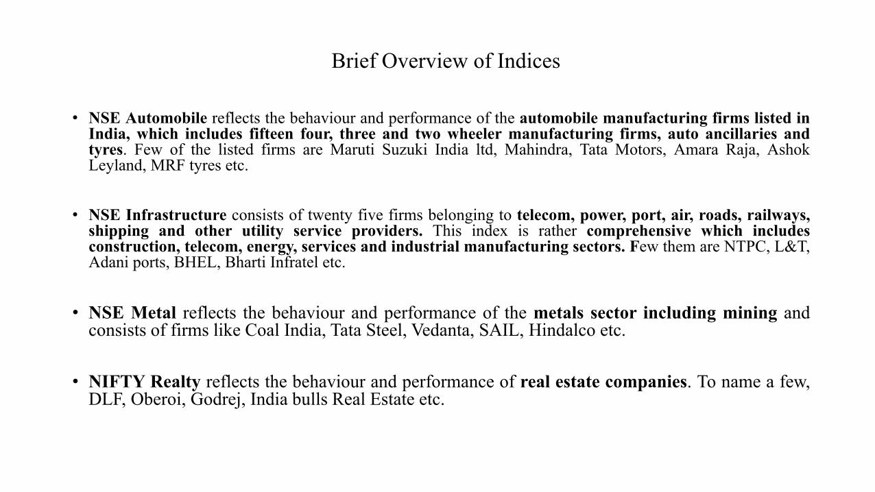
• NSE Automobile reflects the behaviour and performance of the automobile manufacturing firms listed inIndia, which includes fifteen four, three and two wheeler manufacturing firms, auto ancillaries andtyres. Few of the listed firms are Maruti Suzuki India ltd, Mahindra, Tata Motors, Amara Raja, AshokLeyland, MRF tyres etc.

• NSE Infrastructure consists of twenty five firms belonging to telecom, power, port, air, roads, railways,shipping and other utility service providers. This index is rather comprehensive which includesconstruction, telecom, energy, services and industrial manufacturing sectors. Few them are NTPC, L&T,Adani ports, BHEL, Bharti Infratel etc.

• NSE Metal reflects the behaviour and performance of the metals sector including mining andconsists of firms like Coal India, Tata Steel, Vedanta, SAIL, Hindalco etc.

• NIFTY Realty reflects the behaviour and performance of real estate companies. To name a few,DLF, Oberoi, Godrej, India bulls Real Estate etc.

Sectoral indices’ statistics Source: Nifty Index Report

NSE Sectoral Index Total return(%) Standard Deviation Correlation with NIFTY 50

Sensitivity to market returns

(Beta, NIFTY 50)NSE AUTO 15.61 24.30 0.82 0.87

NSE INFRA 10.24 26.51 0.90 1.05

NSE METAL 12.74 35.26 0.80 1.23

NSE REALTY -5.54 41.70 0.75 1.40

Methodology

Multi-variate BEKK GARCH (Engle and Kroner,1995)

Returns of all the series are calculated by taking the first differences of the logarithm of the two successive prices i.e. 𝑅𝑅𝑡𝑡 = log( 𝑝𝑝𝑡𝑡

𝑝𝑝𝑡𝑡−1)

Pre-modelling testsADF Unit Root TestARCH effects (LM statistics)

Advantages It overcomes the limitations of diagonal BEKK model to enforce positive-definiteness Its ability to allow for complicated interactions among the variables which was precluded by the structure

of the diagonal models, both VECH and BEKK, where the only thing that determines the variance of oneseries is its own shocks.

It provides the direction, magnitude and persistence of volatility spill-overs.

BEKK Recursion

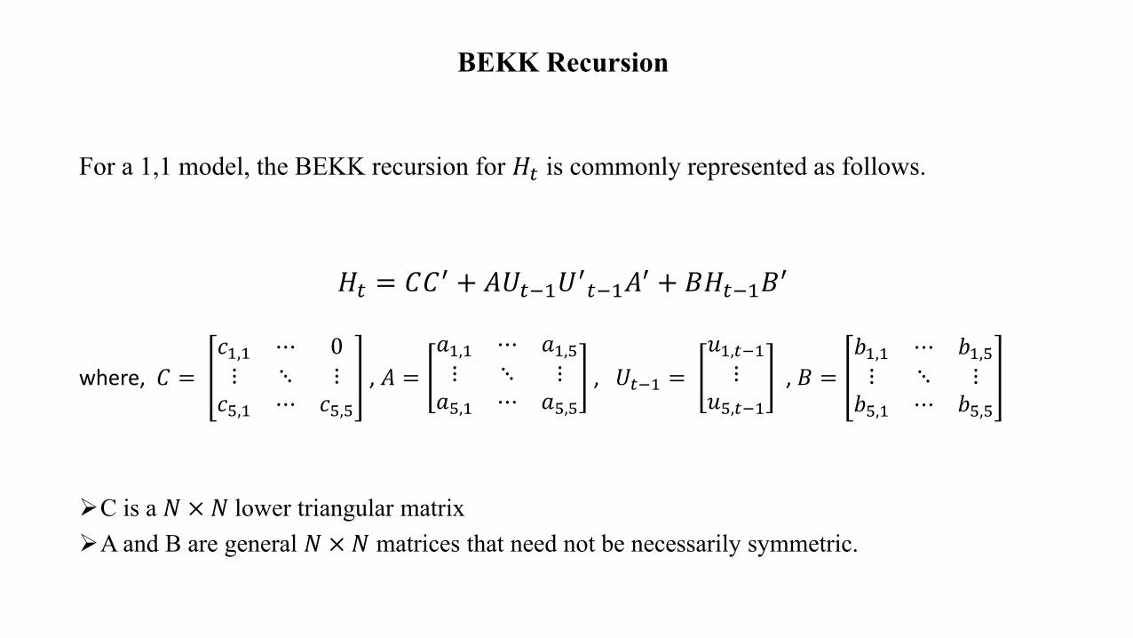
For a 1,1 model, the BEKK recursion for 𝐻𝐻𝑡𝑡 is commonly represented as follows.

𝐻𝐻𝑡𝑡 = 𝐶𝐶𝐶𝐶′ + 𝐴𝐴𝑈𝑈𝑡𝑡−1𝑈𝑈′𝑡𝑡−1𝐴𝐴′ + 𝐵𝐵𝐻𝐻𝑡𝑡−1𝐵𝐵′

where, 𝐶𝐶 =𝑐𝑐1,1 ⋯ 0⋮ ⋱ ⋮𝑐𝑐5,1 ⋯ 𝑐𝑐5,5

, 𝐴𝐴 =𝑎𝑎1,1 ⋯ 𝑎𝑎1,5⋮ ⋱ ⋮

𝑎𝑎5,1 ⋯ 𝑎𝑎5,5

, 𝑈𝑈𝑡𝑡−1 =𝑢𝑢1,𝑡𝑡−1⋮

𝑢𝑢5,𝑡𝑡−1

, 𝐵𝐵 =𝑏𝑏1,1 ⋯ 𝑏𝑏1,5⋮ ⋱ ⋮𝑏𝑏5,1 ⋯ 𝑏𝑏5,5

C is a 𝑁𝑁 × 𝑁𝑁 lower triangular matrixA and B are general 𝑁𝑁 × 𝑁𝑁 matrices that need not be necessarily symmetric.

Since our empirical exercise deals with five variables in an equation at a time (one sectoralindex return and four base metal futures’ returns), we have illustrated a representation ofBEKK system of equation with N=5. Here ‘i’, ‘j’, ‘t’ represent the sectoral NSE indices,commodity futures and time-period respectively.

For such an equation,

𝐻𝐻𝑖𝑖,𝑗𝑗,𝑡𝑡 =𝜎𝜎1,1,𝑡𝑡−12 ⋯ 𝜎𝜎1,5,𝑡𝑡−1

2

⋮ ⋱ ⋮𝜎𝜎5,1,𝑡𝑡−12 ⋯ 𝜎𝜎5,5,𝑡𝑡−1

2

𝐶𝐶 =𝑐𝑐1,1 ⋯ 0⋮ ⋱ ⋮𝑐𝑐5,1 ⋯ 𝑐𝑐5,5

, 𝐴𝐴 =𝑎𝑎1,1 ⋯ 𝑎𝑎1,5⋮ ⋱ ⋮

𝑎𝑎5,1 ⋯ 𝑎𝑎5,5

, 𝑈𝑈𝑡𝑡−1 =𝑢𝑢1,𝑡𝑡−1⋮

𝑢𝑢5,𝑡𝑡−1

, 𝐵𝐵 =𝑏𝑏1,1 ⋯ 𝑏𝑏1,5⋮ ⋱ ⋮𝑏𝑏5,1 ⋯ 𝑏𝑏5,5

The matrix form of the same equation is elaborated as follows,

𝐻𝐻𝑡𝑡

=𝑐𝑐1,1 ⋯ 0⋮ ⋱ ⋮𝑐𝑐5,1 ⋯ 𝑐𝑐5,5

𝑐𝑐1,1 ⋯ 𝑐𝑐5,1⋮ ⋱ ⋮𝑐𝑐1,5 ⋯ 𝑐𝑐5,5

+𝑎𝑎1,1 ⋯ 𝑎𝑎1,5⋮ ⋱ ⋮

𝑎𝑎5,1 ⋯ 𝑎𝑎5,5

𝑢𝑢1,𝑡𝑡−1⋮

𝑢𝑢5,𝑡𝑡−1

𝑢𝑢1,𝑡𝑡−1 ⋯ 𝑢𝑢5,𝑡𝑡−1

𝑎𝑎1,1 ⋯ 𝑎𝑎5,1⋮ ⋱ ⋮

𝑎𝑎1,5 ⋯ 𝑎𝑎5,5

+𝑏𝑏1,1 ⋯ 𝑏𝑏1,5⋮ ⋱ ⋮𝑏𝑏5,1 ⋯ 𝑏𝑏5,5

𝜎𝜎1,1,𝑡𝑡−12 ⋯ 𝜎𝜎1,5,𝑡𝑡−1

2

⋮ ⋱ ⋮𝜎𝜎5,1,𝑡𝑡−12 ⋯ 𝜎𝜎5,5,𝑡𝑡−1

2

𝑏𝑏1,1 ⋯ 𝑏𝑏5,1⋮ ⋱ ⋮𝑏𝑏1,5 ⋯ 𝑏𝑏5,5

=𝑐𝑐1,1 ⋯ 0⋮ ⋱ ⋮𝑐𝑐5,1 ⋯ 𝑐𝑐5,5

𝑐𝑐1,1 ⋯ 𝑐𝑐5,1⋮ ⋱ ⋮𝑐𝑐1,5 ⋯ 𝑐𝑐5,5

+𝑎𝑎1,1 ⋯ 𝑎𝑎1,5⋮ ⋱ ⋮

𝑎𝑎5,1 ⋯ 𝑎𝑎5,5

𝑢𝑢1,𝑡𝑡−12 ⋯ 𝑢𝑢1,𝑡𝑡−1𝑢𝑢5,𝑡𝑡−1⋮ ⋱ ⋮

𝑢𝑢5,𝑡𝑡−1𝑢𝑢1,𝑡𝑡−1 ⋯ 𝑢𝑢2,𝑡𝑡−12

𝑎𝑎1,1 ⋯ 𝑎𝑎5,1⋮ ⋱ ⋮

𝑎𝑎1,5 ⋯ 𝑎𝑎5,5

+𝑏𝑏1,1 ⋯ 𝑏𝑏1,5⋮ ⋱ ⋮𝑏𝑏5,1 ⋯ 𝑏𝑏5,5

𝜎𝜎1,1,𝑡𝑡−12 ⋯ 𝜎𝜎1,5,𝑡𝑡−1

2

⋮ ⋱ ⋮𝜎𝜎5,1,𝑡𝑡−12 ⋯ 𝜎𝜎5,5,𝑡𝑡−1

2

𝑏𝑏1,1 ⋯ 𝑏𝑏5,1⋮ ⋱ ⋮𝑏𝑏1,5 ⋯ 𝑏𝑏5,5

Methodology

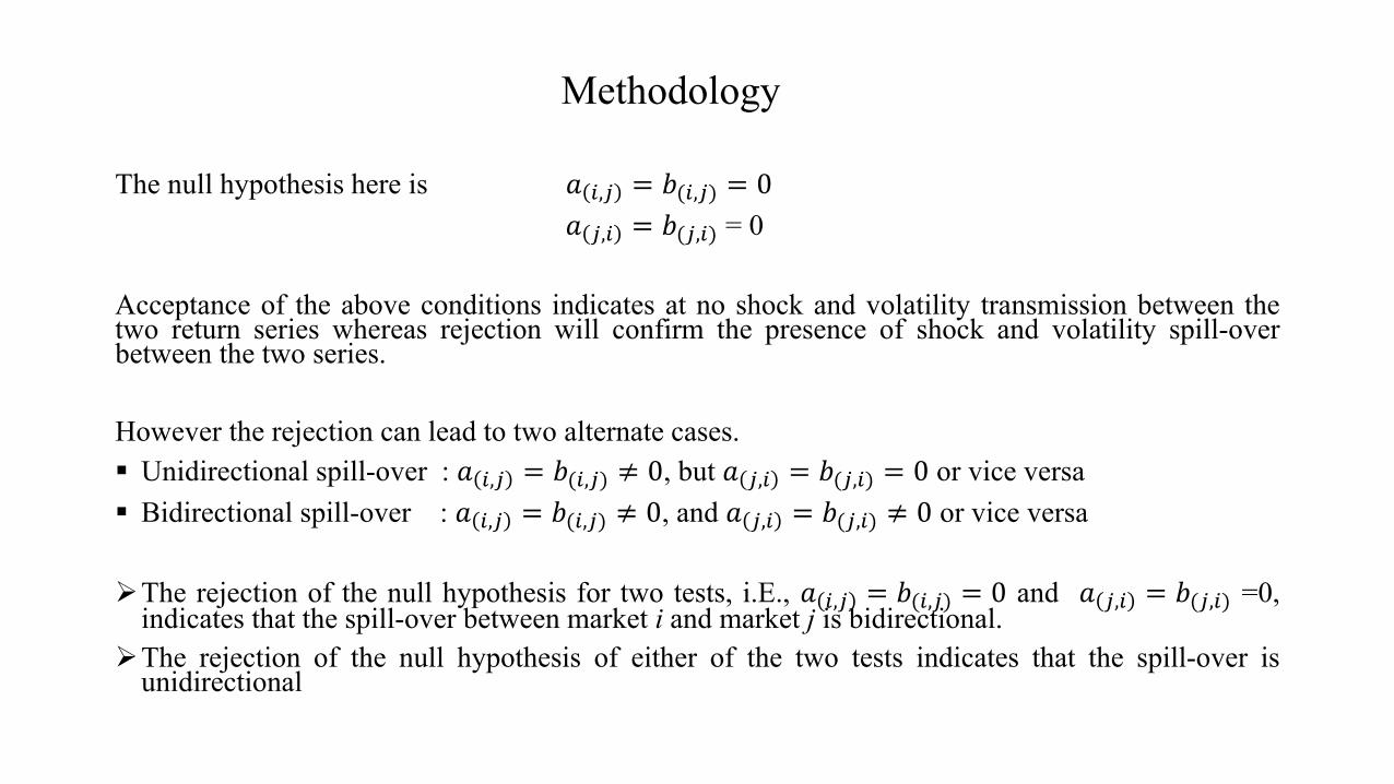
The null hypothesis here is 𝑎𝑎 𝑖𝑖,𝑗𝑗 = 𝑏𝑏(𝑖𝑖,𝑗𝑗) = 0𝑎𝑎 𝑗𝑗,𝑖𝑖 = 𝑏𝑏(𝑗𝑗,𝑖𝑖) = 0

Acceptance of the above conditions indicates at no shock and volatility transmission between thetwo return series whereas rejection will confirm the presence of shock and volatility spill-overbetween the two series.

However the rejection can lead to two alternate cases. Unidirectional spill-over : 𝑎𝑎 𝑖𝑖,𝑗𝑗 = 𝑏𝑏(𝑖𝑖,𝑗𝑗) ≠ 0, but 𝑎𝑎 𝑗𝑗,𝑖𝑖 = 𝑏𝑏(𝑗𝑗,𝑖𝑖) = 0 or vice versa Bidirectional spill-over : 𝑎𝑎 𝑖𝑖,𝑗𝑗 = 𝑏𝑏(𝑖𝑖,𝑗𝑗) ≠ 0, and 𝑎𝑎 𝑗𝑗,𝑖𝑖 = 𝑏𝑏(𝑗𝑗,𝑖𝑖) ≠ 0 or vice versa

The rejection of the null hypothesis for two tests, i.E., 𝑎𝑎 𝑖𝑖,𝑗𝑗 = 𝑏𝑏(𝑖𝑖,𝑗𝑗) = 0 and 𝑎𝑎 𝑗𝑗,𝑖𝑖 = 𝑏𝑏(𝑗𝑗,𝑖𝑖) =0,indicates that the spill-over between market i and market j is bidirectional.

The rejection of the null hypothesis of either of the two tests indicates that the spill-over isunidirectional

Table 1. Full BEKK estimates for automobile index returns

Notes: (1) C = 𝑐𝑐11 ⋯ 𝑐𝑐15⋮ ⋱ ⋮0 0 𝑐𝑐55

A = 𝑎𝑎11 ⋯ 𝑎𝑎15⋮ ⋱ ⋮𝑎𝑎51 𝑎𝑎53 𝑎𝑎55

, B = 𝑏𝑏11 ⋯ 𝑏𝑏15⋮ ⋱ ⋮𝑏𝑏51 𝑏𝑏53 𝑏𝑏55

(2) The entries for section C, A and section B are the covariance coefficients of constant, residual interaction terms (ARCH) and volatility spill-over GARCH (1,1) respectively followed by the standard errors in parentheses. These coefficients are derived from equations given below(3) ***, **, * represent the level of significance at 1%, 5% and 10% respectively.

Table 3.Full BEKK

C A B

Coeff.(c)

Auto Alu Zinc Nickel Lead Coeff.(a)

Auto Alu Zinc Nickel Lead Coeff.(b)

Auto Alu Zinc Nickel Lead

Auto 0.002***(0.000)

0.000**(0.000)

0.000*(0.000)

0.000***(0.000)

0.000**(0.000)

Auto 0.266***(0.017)

0.008*(0.004)

0.002(0.005)

0.016**(0.006)

0.006(0.006)

Auto 0.943***(0.007)

-0.004**(0.001)

-0.003(0.002)

-0.007***(0.002)

-0.004**(0.002)

Alu 0.000***(0.000)

0.000***(0.000)

0.000***(0.000)

0.000***(0.000)

Alu 0.011(0.019)

0.223***(0.015)

0.029**(0.015)

0.066***(0.017)

-0.003(0.018)

Alu -0.005(0.006)

0.967***(0.004)

-0.010**(0.004)

-0.015***(0.004)

0.001(0.005)

Zinc -0.000(0.000)

0.000(0.000)

0.000(0.000)

Zinc 0.009(0.021)

-0.035***(0.012)

0.147***(0.016)

-0.053***(0.017)

0.004(0.018)

Zinc 0.001(0.004)

0.007***(0.002)

0.988***(0.003)

0.007**(0.003)

-0.004(0.004)

Nickel 0.000**(0.000)

0.000(0.000)

Nickel 0.043**(0.020)

0.017**(0.007)

0.036***(0.009)

0.162***(0.010)

0.048***(0.009)

Nickel -0.010***(0.004)

-0.003**(0.001)

-0.004**(0.001)

0.985***(0.001)

-0.007***(0.001)

Lead 0.000(0.000)

Lead -0.029(0.022)

-0.001(0.010)

-0.019(0.015)

0.017(0.013)

0.136***(0.015)

Lead 0.005(0.005)

-0.001(0.002)

0.004(0.003)

-0.002(0.002)

0.990***(0.002)

Table 2. Full BEKK estimates for infrastructure index returns

Notes: (1) C = 𝑐𝑐11 ⋯ 𝑐𝑐15⋮ ⋱ ⋮0 0 𝑐𝑐55

A = 𝑎𝑎11 ⋯ 𝑎𝑎15⋮ ⋱ ⋮𝑎𝑎51 𝑎𝑎53 𝑎𝑎55

, B = 𝑏𝑏11 ⋯ 𝑏𝑏15⋮ ⋱ ⋮𝑏𝑏51 𝑏𝑏53 𝑏𝑏55

(2) The entries for section C, A and section B are the covariance coefficients of constant, residual interaction terms and volatility spill-over GARCH (1,1) respectively followed by the standard errors in parentheses. These coefficients are derived from equations given below(3) ***, **, * represent the level of significance at 1%, 5% and 10% respectively.

Table 4.full BEKK

C A B

Coeff.(c)

Infra Alu Zinc Nickel Lead Coeff.(a)

Infra Alu Zinc Nickel Lead Coeff.(b)

Infra Alu Zinc Nickel Lead

Infra 0.002***(0.000)

0.001(0.000)

-0.002***(0.00)

-0.000(0.001)

-0.002**(0.001)

Infra 0.350***(0.019)

-0.005**(0.002)

-0.005(0.003)

0.005(0.004)

0.002(0.003)

Infra 0.921***(0.008)

0.003***(0.001)

0.002**(0.001)

-0.000(0.552)

0.000(0.626)

Alu 0.001**(0.001)

0.001(0.002)

0.002(0.001)

0.002(0.002)

Alu -0.038**(0.016)

0.165***(0.009)

0.003(0.009)

0.070***(0.011)

0.053***(0.010)

Alu 0.009**(0.024)

0.984***(0.001)

-0.001(0.001)

-0.009***(0.002)

-0.012***(0.002)

Zinc -0.000(0.003)

-0.000(0.002)

-0.000(0.003)

Zinc -0.003(0.018)

-0.016**(0.007)

0.166***(0.008)

-0.099***(0.012)

-0.012(0.011)

Zinc 0.002(0.004)

0.000(0.001)

0.983***(0.001)

0.025***(0.002)

-0.003(0.002)

Nickel -0.000(0.001)

0.000(0.000)

Nickel 0.013(0.015)

0.017***(0.004)

0.032***(0.006)

0.133***(0.007)

0.003(0.007)

Nickel -0.005*(0.091)

-0.003***(0.000)

-0.006**(0.001)

0.986***(0.001)

0.011***(0.001)

Lead 0.000(0.000)

Lead 0.003(0.016)

-0.014**(0.006)

-0.043***(0.009)

0.033***(0.011)

0.115***(0.009)

Lead 0.004(0.257)

0.002**(0.001)

0.010***(0.001)

-0.017***(0.002)

0.990***(0.001)

Table 3. Full BEKK estimates for metal sector returns

Notes: (1) C = 𝑐𝑐11 ⋯ 𝑐𝑐15⋮ ⋱ ⋮0 0 𝑐𝑐55

A = 𝑎𝑎11 ⋯ 𝑎𝑎15⋮ ⋱ ⋮

𝑎𝑎5,1 𝑎𝑎53 𝑎𝑎55, B =

𝑏𝑏11 ⋯ 𝑏𝑏15⋮ ⋱ ⋮𝑏𝑏5,1 𝑏𝑏53 𝑏𝑏55

(2) The entries for section C, A and section B are the covariance coefficients of constant, residual interaction terms and volatility spill-over GARCH (1,1) respectively, followed by the standard errors in parentheses. These coefficients are derived from equations given below(3) ***, **, * represent the level of significance at 1%, 5% and 10% respectively.

Table 5.Full BEKK

C A B

Coeff.(c)

Metal Alu Zinc Nickel Lead Coeff.(a)

Metal Alu Zinc Nickel Lead Coeff.(b)

Metal Alu Zinc Nickel Lead

Metal -0.012***(0.000)

-0.000(0.000)

-0.000(0.000)

-0.000(0.000)

-0.000(0.000)

Metal 0.666***(0.028)

-0.000(0.000)

0.000(0.000)

-0.000(0.000)

0.000(0.000)

Metal -0.410***(0.089)

0.000(0.000)

-0.000(0.000)

0.000(0.000)

-0.000(0.000)

Alu 0.000***(0.000)

0.000**(0.000)

0.000***(0.000)

0.000***(0.000)

Alu -0.112*(0.063)

0.192***(0.012)

-0.002(0.013)

0.027(0.018)

0.104***(0.014)

Alu 0.182**(0.075)

0.980***(0.002)

0.010***(0.003)

-0.009**(0.004)

-0.040***(0.004)

Zinc 0.000(0.000)

-0.000(0.000)

0.000(0.000)

Zinc 0.002(0.059)

-0.016(0.017)

0.137***(0.018)

-0.053(0.055)

-0.104***(0.019)

Zinc 0.081(0.070)

-0.012***(0.004)

1.000***(0.004)

0.008(0.014)

0.070(0.004)

Nickel 0.000(0.000)

0.000(0.000)

Nickel -0.186**(0.075)

0.033***(0.010)

0.052***(0.011)

0.167***(0.012)

0.030**(0.014)

Nickel 0.115**(0.052)

-0.002(0.001)

-0.004(0.003)

0.986***(0.002)

-0.010***(0.002)

Lead -0.000(0.000)

Lead 0.108(0.076)

-0.046***(0.013)

-0.031**(0.014)

0.004(0.045)

0.091***(0.075)

Lead -0.145**(0.059)

0.014***(0.003)

-0.037***(0.003)

-0.002(0.011)

0.963***(0.003)

Table 4. Full BEKK results for realty sector returns

Notes: (1) C = 𝑐𝑐11 ⋯ 𝑐𝑐15⋮ ⋱ ⋮0 0 𝑐𝑐55

A = 𝑎𝑎11 ⋯ 𝑎𝑎15⋮ ⋱ ⋮𝑎𝑎51 𝑎𝑎53 𝑎𝑎55

, B = 𝑏𝑏11 ⋯ 𝑏𝑏15⋮ ⋱ ⋮𝑏𝑏51 𝑏𝑏53 𝑏𝑏55

(2) The entries for section C, A and section B are the covariance coefficients of constant, residual interaction terms and GARCH (1,1) respectively followed by the standard errors in parentheses. These coefficients are derived from equations given below(3) ***, **, * represent the level of significance at 1%, 5% and 10% respectively. Source : Author’s own calculation

Table 6.Full BEKK

A A B

Coeff.(c)

Realty Alu Zinc Nickel Lead Coeff.(a)

Realty Alu Zinc Nickel Lead Coeff.(b)

Realty Alu Zinc Nickel Lead

Realty 0.007***(0.000)

-0.000***(0.000)

-0.000(0.000)

0.000(0.000)

-0.000**(0.000)

Realty 0.423***(0.025)

0.001(0.002)

0.002(0.002)

0.010***(0.002)

0.005*(0.002)

Realty 0.869***(0.016)

0.001(0.001)

-0.000(0.001)

-0.003**(0.001)

-0.000(0.001)

Alu 0.000***(0.000)

0.000***(0.000)

0.000***(0.000)

0.000***(0.000)

Alu -0.071**(0.032)

0.212***(0.013)

-0.003(0.012)

0.055***(0.015)

-0.004(0.015)

Alu 0.008(0.009)

0.973***(0.002)

-0.004(0.002)

-0.014***(0.003)

0.005(0.003)

Zinc 0.000(0.000)

-0.000(0.000)

-0.000(0.000)

Zinc -0.052(0.039)

-0.037***(0.011)

0.146***(0.012)

-0.056***(0.019)

0.033**(0.015)

Zinc 0.013*(0.007)

0.007**(0.002)

0.985***(0.002)

0.005(0.003)

-0.013***(0.003)

Nickel 0.000(0.000)

0.000(0.000)

Nickel 0.006(0.030)

0.017***(0.006)

-0.053***(0.007)

0.157***(0.009)

0.054***(0.018)

Nickel -0.004(0.007)

-0.002**(0.001)

-0.006***(0.001)

0.986***(0.001)

-0.008***(0.002)

Lead 0.000(0.000)

Lead 0.068**(0.033)

-0.008(0.007)

-0.007(0.008)

0.018(0.011)

0.097***(0.009)

Lead 0.007(0.007)

-0.001(0.001)

0.005***(0.001)

0.001(0.001)

0.997***(0.001)

Graphs representing covariances between base metal futures and industrial sectors

Automobile Infrastructure Metal Real Estate

Results

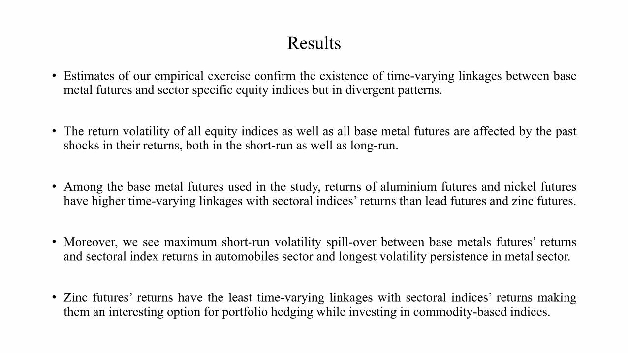
• Estimates of our empirical exercise confirm the existence of time-varying linkages between basemetal futures and sector specific equity indices but in divergent patterns.

• The return volatility of all equity indices as well as all base metal futures are affected by the pastshocks in their returns, both in the short-run as well as long-run.

• Among the base metal futures used in the study, returns of aluminium futures and nickel futureshave higher time-varying linkages with sectoral indices’ returns than lead futures and zinc futures.

• Moreover, we see maximum short-run volatility spill-over between base metals futures’ returnsand sectoral index returns in automobiles sector and longest volatility persistence in metal sector.

• Zinc futures’ returns have the least time-varying linkages with sectoral indices’ returns makingthem an interesting option for portfolio hedging while investing in commodity-based indices.

Implications

Commodity futures retain scope for portfolio diversification as each of the base metals displayunique linkages in terms of direction, magnitude and volatility persistence.

It is evident that negative shocks have greater impact on volatility spill-overs between the market thanpositive shocks of the same magnitude.

Shocks to the returns of base metal futures are capable of fuelling persistent volatility in the returns ofsectoral equity indices confirming that supply-side information leads to the transmission ofvolatility between equity and commodities.

Importantly, our study confirms the economic channel of sector-specific demand and commodity-specific supply are possible channels of commodity-equity linkage. Overall our results are aligningwith the results obtained by Lee and Ni (2002) and Malik and Ewing (2009).

Thank You