commodity options pricing by the fourier space time-stepping method · commodity options pricing by...

Commodity Options Pricing by theFourier Space Time-stepping Method

by

Chunhao Shan

A research paperpresented to the University of Waterloo

in partial fulfillment of therequirement for the degree of

Master of Mathematicsin

Computational Mathematics

Supervisors: Prof. Peter Forsyth & Prof. George Labahn

Waterloo, Ontario, Canada, 2014

c© Chunhao Shan 2014

I hereby declare that I am the sole author of this report. This is a true copy of the report,including any required final revisions, as accepted by my examiners.

I understand that my report may be made electronically available to the public.

ii

Abstract

We study the framework of the Fourier space time-stepping (FST) method for pric-ing contingent claims in financial markets. By using the semi-Lagrangian method, theFST method is extended to the pricing of commodity contingent claims. We study thecommodity one-factor and two-factor models and the related semi-Lagrangian schemes forthese models. Numerical results of pricing commodity European and American options arepresented.

iii

Acknowledgements

I would like to thank my supervisors, Prof. Peter Forsyth and Prof. George Labahn,for their guidance, patience and support throughout the year. I would also like to thankmy family and friends.

iv

Dedication

This is dedicated to my parents.

v

Table of Contents

List of Tables viii

List of Figures xii

List of Algorithms xiii

1 Introduction 1

2 Mathematical Models 4

2.1 Black-Scholes-Merton Model . . . . . . . . . . . . . . . . . . . . . . . . . . 4

2.2 Commodity Price Models . . . . . . . . . . . . . . . . . . . . . . . . . . . . 5

2.2.1 One-factor Model . . . . . . . . . . . . . . . . . . . . . . . . . . . . 6

2.2.2 Two-factor Model . . . . . . . . . . . . . . . . . . . . . . . . . . . . 6

3 Fourier Space Time-stepping Method 9

3.1 Introduction . . . . . . . . . . . . . . . . . . . . . . . . . . . . . . . . . . . 9

3.1.1 Continuous Fourier Transform . . . . . . . . . . . . . . . . . . . . . 9

3.1.2 Discrete Fourier Transform . . . . . . . . . . . . . . . . . . . . . . . 10

3.2 FST Algorithm for Options under the BSM Model . . . . . . . . . . . . . . 13

3.2.1 Fully Implicit and Crank-Nicolson . . . . . . . . . . . . . . . . . . . 16

3.2.2 FST for European Option under the BSM Model . . . . . . . . . . 19

3.2.3 FST for American Option under the BSM Model . . . . . . . . . . 21

vi

4 Semi-Lagrangian Method 23

4.1 Advection-diffusion Equation with Constant Velocity . . . . . . . . . . . . 23

4.2 Advection-diffusion Equation with Non-constant Velocity . . . . . . . . . . 24

4.3 Application to the Commodity Price Models . . . . . . . . . . . . . . . . . 27

4.4 Interpolation Methods . . . . . . . . . . . . . . . . . . . . . . . . . . . . . 29

4.5 Error of the Semi-Lagrangian Method . . . . . . . . . . . . . . . . . . . . . 31

5 Numerical Results 32

5.1 Commodity Options under a One-factor Model . . . . . . . . . . . . . . . . 32

5.1.1 FST Algorithm for Options under a One-factor Model . . . . . . . . 32

5.1.2 Monte Carlo for European Option under a One-factor Model . . . . 36

5.1.3 FST for European Option under a One-factor Model . . . . . . . . 36

5.1.4 FST for American Option under a One-factor Model . . . . . . . . 40

5.2 Commodity Options under a Two-factor Model . . . . . . . . . . . . . . . 43

5.2.1 FST Algorithm for Options under a Two-factor Model . . . . . . . 43

5.2.2 Monte Carlo for European Option under a Two-factor Model . . . . 47

5.2.3 FST for European Option under a Two-factor Model . . . . . . . . 47

5.2.4 FST for American Option under a Two-factor Model . . . . . . . . 51

6 Conclusions 53

APPENDICES 55

A Wrap-around Error 56

References 59

vii

List of Tables

3.1 Single asset option parameters under BSM model. . . . . . . . . . . . . . . 20

3.2 Single asset European put under BSM model, FST with fully implicit, closedform solution = 3.75341839, first order convergence, including both spaceand time errors. . . . . . . . . . . . . . . . . . . . . . . . . . . . . . . . . . 20

3.3 Single asset European put under BSM model, FST with Crank-Nicolson,closed form solution = 3.75341839, second order convergence, including bothspace and time errors. . . . . . . . . . . . . . . . . . . . . . . . . . . . . . 20

3.4 Single asset American put under BSM model, FST with fully implicit, firstorder convergence, including both space and time errors. . . . . . . . . . . 21

3.5 Single asset American put under BSM model, FST with Crank-Nicolson,first order convergence, including both space and time errors. . . . . . . . . 22

3.6 Single asset American put under BSM model, finite difference with fullyimplicit (not vectorized), first order convergence, including both space andtime errors. . . . . . . . . . . . . . . . . . . . . . . . . . . . . . . . . . . . 22

3.7 Single asset American put under BSM model, finite difference with Crank-Nicolson (not vectorized), first order convergence, including both space andtime errors. . . . . . . . . . . . . . . . . . . . . . . . . . . . . . . . . . . . 22

5.1 Single asset commodity option parameters under one-factor model. . . . . 36

5.2 Single asset commodity European call under one-factor model, Monte Carlo. 36

5.3 Single asset commodity European call under one-factor model, fully implicitwith linear interpolation, Monte Carlo solution = 0.87940762 (standard error= 0.00435362), first order convergence, including both space and time errors. 37

viii

5.4 Single asset commodity European call under one-factor model, fully implicitwith piecewise quadratic interpolation (not vectorized), Monte Carlo solu-tion = 0.87940762 (standard error = 0.00435362), first order convergence,including both space and time errors. . . . . . . . . . . . . . . . . . . . . . 37

5.5 Single asset commodity European call under one-factor model, fully implicitwith cubic spline interpolation, Monte Carlo solution = 0.87940762 (stan-dard error = 0.00435362), first order convergence, including both space andtime errors. . . . . . . . . . . . . . . . . . . . . . . . . . . . . . . . . . . . 37

5.6 Single asset commodity European call under one-factor model, Crank-Nicolsonwith linear interpolation, Monte Carlo solution = 0.87940762 (standard er-ror = 0.00435362), first order convergence, including both space and timeerrors. . . . . . . . . . . . . . . . . . . . . . . . . . . . . . . . . . . . . . . 38

5.7 Single asset commodity European call under one-factor model, Crank-Nicolsonwith piecewise quadratic interpolation (not vectorized), Monte Carlo solu-tion = 0.87940762 (standard error = 0.00435362), second order convergence,including both space and time errors. . . . . . . . . . . . . . . . . . . . . . 38

5.8 Single asset commodity European call under one-factor model, Crank-Nicolsonwith cubic spline interpolation, Monte Carlo solution = 0.87940762 (stan-dard error = 0.00435362), second order convergence, including both spaceand time errors. . . . . . . . . . . . . . . . . . . . . . . . . . . . . . . . . . 39

5.9 Single asset commodity American call under one-factor model, fully implicitwith linear interpolation, first order convergence, including both space andtime errors. . . . . . . . . . . . . . . . . . . . . . . . . . . . . . . . . . . . 40

5.10 Single asset commodity American call under one-factor model, fully implicitwith piecewise quadratic interpolation (not vectorized), first order conver-gence, including both space and time errors. . . . . . . . . . . . . . . . . . 40

5.11 Single asset commodity American call under one-factor model, fully implicitwith cubic spline interpolation, first order convergence, including both spaceand time errors. . . . . . . . . . . . . . . . . . . . . . . . . . . . . . . . . . 41

5.12 Single asset commodity American call under one-factor model, Crank-Nicolsonwith linear interpolation, first order convergence, including both space andtime errors. . . . . . . . . . . . . . . . . . . . . . . . . . . . . . . . . . . . 42

5.13 Single asset commodity American call under one-factor model, Crank-Nicolsonwith piecewise quadratic interpolation (not vectorized), first order conver-gence, including both space and time errors. . . . . . . . . . . . . . . . . . 42

ix

5.14 Single asset commodity American call under one-factor model, Crank-Nicolsonwith cubic spline interpolation, first order convergence, including both spaceand time errors. . . . . . . . . . . . . . . . . . . . . . . . . . . . . . . . . . 42

5.15 Single asset commodity option parameters under two-factor model. . . . . 47

5.16 Single asset commodity European put under two-factor model, Monte Carlo. 47

5.17 Single asset commodity European put under two-factor model, fully implicitwith linear interpolation, Monte Carlo solution = 1.10497142 (standard error= 0.00477254), first order convergence, including both space and time errors. 48

5.18 Single asset commodity European put under two-factor model, fully implicitwith piecewise quadratic interpolation (not vectorized), Monte Carlo solu-tion = 1.10497142 (standard error = 0.00477254), first order convergence,including both space and time errors. . . . . . . . . . . . . . . . . . . . . . 48

5.19 Single asset commodity European put under two-factor model, fully implicitwith cubic spline interpolation, Monte Carlo solution = 1.10497142 (stan-dard error = 0.00477254), first order convergence, including both space andtime errors. . . . . . . . . . . . . . . . . . . . . . . . . . . . . . . . . . . . 48

5.20 Single asset commodity European put under two-factor model, Crank-Nicolsonwith linear interpolation, Monte Carlo solution = 1.10497142 (standard er-ror = 0.00477254), first order convergence, including both space and timeerrors. . . . . . . . . . . . . . . . . . . . . . . . . . . . . . . . . . . . . . . 49

5.21 Single asset commodity European put under two-factor model, Crank-Nicolsonwith piecewise quadratic interpolation (not vectorized), Monte Carlo solu-tion = 1.10497142 (standard error = 0.00477254), second order convergence,including both space and time errors. . . . . . . . . . . . . . . . . . . . . . 49

5.22 Single asset commodity European put under two-factor model, Crank-Nicolsonwith cubic spline interpolation, Monte Carlo solution = 1.10497142 (stan-dard error = 0.00477254), second order convergence, including both spaceand time errors. . . . . . . . . . . . . . . . . . . . . . . . . . . . . . . . . . 50

5.23 Single asset commodity American put under two-factor model, fully implicitwith linear interpolation, first order convergence, including both space andtime errors. . . . . . . . . . . . . . . . . . . . . . . . . . . . . . . . . . . . 51

5.24 Single asset commodity American put under two-factor model, fully implicitwith piecewise quadratic interpolation (not vectorized), first order conver-gence, including both space and time errors. . . . . . . . . . . . . . . . . . 51

x

5.25 Single asset commodity American put under two-factor model, fully implicitwith cubic spline interpolation, first order convergence, including both spaceand time errors. . . . . . . . . . . . . . . . . . . . . . . . . . . . . . . . . . 51

5.26 Single asset commodity American put under two-factor model, Crank-Nicolsonwith linear interpolation, first order convergence, including both space andtime errors. . . . . . . . . . . . . . . . . . . . . . . . . . . . . . . . . . . . 52

5.27 Single asset commodity American put under two-factor model, Crank-Nicolsonwith piecewise quadratic interpolation (not vectorized), first order conver-gence, including both space and time errors. . . . . . . . . . . . . . . . . . 52

5.28 Single asset commodity American put under two-factor model, Crank-Nicolsonwith cubic spline interpolation, first order convergence, including both spaceand time errors. . . . . . . . . . . . . . . . . . . . . . . . . . . . . . . . . . 52

A.1 Single asset option parameters under BSM model. . . . . . . . . . . . . . . 58

A.2 Single asset European call under BSM model, wrap-around error. . . . . . 58

xi

List of Figures

3.1 Approximation for the discrete Fourier transform. . . . . . . . . . . . . . . 12

3.2 Approximation for the inverse discrete Fourier transform. . . . . . . . . . . 13

4.1 Semi-Lagrangian scheme. . . . . . . . . . . . . . . . . . . . . . . . . . . . . 26

4.2 Linear interpolation and piecewise quadratic interpolation. . . . . . . . . . 30

xii

List of Algorithms

1 FST with fully implicit for single asset option under BSM model. . . . . . . 18

2 FST with Crank-Nicolson for single asset option under BSM model. . . . . . 19

3 FST with fully implicit for single asset commodity option under one-factormodel. . . . . . . . . . . . . . . . . . . . . . . . . . . . . . . . . . . . . . . . 34

4 FST with Crank-Nicolson for single asset commodity option under one-factormodel. . . . . . . . . . . . . . . . . . . . . . . . . . . . . . . . . . . . . . . . 35

5 FST with fully implicit for single asset commodity option under two-factormodel. . . . . . . . . . . . . . . . . . . . . . . . . . . . . . . . . . . . . . . . 45

6 FST with Crank-Nicolson for single asset commodity option under two-factormodel. . . . . . . . . . . . . . . . . . . . . . . . . . . . . . . . . . . . . . . . 46

7 FST with fully implicit for single asset option under BSM model (with zeropadding). . . . . . . . . . . . . . . . . . . . . . . . . . . . . . . . . . . . . . 57

xiii

Chapter 1

Introduction

In finance, a derivative is a type of contract whose price is dependent on and derived from aparticular underlying asset or a basket of underlying assets. The most common underlyingassets include stocks, bonds, commodities, currencies, interest rates and market indexes. Aderivative is generally used to insure against the risk of price movement, which is usuallycalled hedging. It can also be used in many other areas in financial markets, even forspeculative purposes.

Options, futures contracts, forward contracts and swaps are the most common types ofderivatives. An option is a type of contract which gives the owner the right, but not theobligation, to buy or sell an underlying asset or instrument at a specified strike price on orbefore a specified date (maturity). An option that can only be exercised on expiration iscalled a European option. The type of option which gives the owner the right to exerciseon any trading day before expiry is called an American option. A futures contract is acontract between two parties to buy or sell a specified asset of standardized quantity andquality for a price agreed upon today (futures price) with delivery and payment occurringat a specified future date, the delivery date.

As various types of financial derivatives play more significant roles in financial markets,accurate and efficient methods to value derivative contracts are in high demand. TheBlack-Scholes model was first proposed by Black and Scholes (1973) [1]. In this model,they assume the underlying asset price follows a geometric Brownian motion, which de-scribes the stochastic behaviour of the underlying asset. They then determine the price asthe solution of a partial differential equation (PDE). Based on this Black-Scholes partial

1

differential equation, there are various numerical methods to solve the valuation of theoption, such as finite difference, finite volume and finite element methods.

The Fourier space time-stepping method was first developed by Jackson, Jaimungal andSurkov (2008) [6]. This method uses the Fourier transform to numerically solve the partialdifferential equation. The continuous Fourier transform is a linear operator which mapsspatial derivatives into multiplications in Fourier space. Due to convenient properties ofthe Fourier transform, we can convert the valuation in real space to Fourier space, wherethe partial differential equation will become an ordinary differential equation (ODE). Wethen have various straightforward methods to solve the ODE. Meanwhile, it is easy toadd constraints or other conditions between two timesteps to allow for using the Fouriertransform method to price American or other path dependent options.

We know that many financial derivatives, such as options, are dependent on the underlyingassets of the stock prices, which can be modelled as a geometric Brownian motion. How-ever, there are also many contingent claims based on commodity prices. Straightforwardly,by assuming interest rates and convenience yields1 are constant, we can extend our pricingmethods for common stock options2 to derivatives based on commodities. However, thisassumption is not very suitable for commodity prices since it implies that the volatilityof future prices3 is equal to the volatility of spot prices4. Intuitively, in a commoditymarket, when prices are relatively high, supply will increase since higher cost producersof the commodity will enter the market. This will put a downward pressure on prices.Conversely, when prices are relatively low, supply will decrease since some of the highercost producers will exit the market. This will put an upward pressure on prices [13]. Theimpact of relative prices on the supply of the commodity will induce mean reversion incommodity prices. Gibson (1990) [4], Ross (1997) [11], and Schwartz (2000) [13] developedmodels that describe mean reversion properties of commodity prices and derived the cor-responding partial differential equations for valuation of the futures and options based oncommodity prices.

1Convenience yield can be seen as the flow of services accruing to the holder of the spot commoditybut not to the owner of a futures contract [13].

2Options whose underlying assets are stock prices.3The market price under the condition that an commodity asset can be bought or sold for delivery in

the future.4The current market price under the condition that an commodity asset is bought or sold for immediate

payment and delivery.

2

In the commodity price models, including one-factor and two-factor models, an Ornstein-Uhlenbeck process is introduced to describe the mean-reverting behaviour of commodityprices. This induces a non-constant drift term in the pricing partial differential equa-tion. In order to solve the option pricing PDE by the Fourier space time-stepping method,we can use the semi-Lagrangian method to deal with the non-constant velocity term inthe advection-diffusion equation [16]. The purpose of this paper is to combine the semi-Lagrangian method and the Fourier space time-stepping method to compute the values ofsome typical options based on commodity prices.

This paper is structured as follows. In Chapter 2, we introduce the Black-Scholes modeland two models for commodity prices. Chapter 3 presents the framework of the Fourierspace time-stepping method and its application to some typical stock options. In Chapter4, we will provide the introduction of the semi-Lagrangian method and its application tocommodity options valuation. Chapter 5 gives the numerical examples for one-factor andtwo-factor models. Chapter 6 lists the conclusions.

3

Chapter 2

Mathematical Models

2.1 Black-Scholes-Merton Model

In the Black-Scholes-Merton (BSM) model [1], the price of an underlying asset is assumed tofollow a geometric Brownian motion. The stochastic differential equation for the underlyingasset price S can be written as:

dS

S= µdt+ σdZ, (2.1)

where:

µ is the drift rate,σ is the volatility,dZ is the increment of a standard Wiener process.

Moreover, by no-arbitrage arguments, we can write the dynamics of the process under theequivalent martingale measure1 as:

dS

S= rdt+ σdZ∗, (2.2)

1Equivalent martingale measure, also called risk-neutral measure, is used in the pricing of financialderivatives due to the fundamental theorem of asset pricing. Under this measure, the current value offinancial assets is equal to their expected payoffs in the future discounted at the risk-free rate.

4

where:

r is the risk-free rate,dZ∗ is the increment of a standard Wiener process

under the equivalent martingale measure.

Let V(S, τ) be the value of a European option where τ is the time to maturity. Assumingthe payoff of the option at maturity V(S, 0) is known, we can derive a partial differentialequation to solve the price of the option by Ito’s Lemma. This is the Black-Scholes equation:

Vτ =1

2σ2S2VSS + rSVS − rV , (2.3)

with the initial condition (for a call):

V(S, 0) = max(S −K, 0), (2.4)

or (for a put):

V(S, 0) = max(K − S, 0). (2.5)

Here K is the strike price.

2.2 Commodity Price Models

Commodity price models are used to describe the stochastic behaviour of the commodityspot price, which is the current market price under the condition that a commodity asset isbought or sold for immediate payment and delivery. Commodity prices are assumed to bemean reverting. A straightforward approach is to use a mean-reverting Ornstein-Uhlenbeckprocess to model the commodity spot price, which is a one-factor model. However, thismodel has an implicit assumption that the convenience yield has a certain relation withthe spot price. The convenience yield can be seen as the flow of services accruing tothe holder of the spot commodity but not to the owner of a futures contract [13]. If welet the convenience yield also follow a mean-reverting Ornstein-Uhlenbeck process that iscorrelated with the spot price, this leads to a two-factor model. Moreover, by assumingthe interest rate is non-constant, we then have a three-factor model. In this paper, we willfocus on one-factor and two-factor models.

5

2.2.1 One-factor Model

We first assume that the interest rate r is constant, and the logarithm of the spot price Sof the commodity follows a mean-reverting Ornstein-Uhlenbeck process:

dS

S= κ(µ− logS)dt+ σdZ, (2.6)

where:

κ is the magnitude of the speed of adjustment, κ > 0,µ is the drift rate,σ is the volatility,dZ is the increment of a standard Wiener process.

By no-arbitrage arguments, we can write the dynamics of the process under the equivalentmartingale measure as:

dS

S= κ(µ− λ− logS)dt+ σdZ∗, (2.7)

where:

λ is the market price of risk,dZ∗ is the increment of a standard Wiener process


Let V(S, τ) be the value of a commodity option price where τ is the time to maturity. Thenby Ito’s Lemma, we can derive a partial differential equation to solve the option price:

Vτ =1

2σ2S2VSS + κ(µ− λ− logS)SVS, (2.8)

with initial condition given in equation (2.4) or (2.5).

2.2.2 Two-factor Model

Unlike the one-factor model, a two-factor model was developed by Gibson and Schwartz(1990) [4]. The first factor is the spot price of the commodity S and the second is the

6

instantaneous convenience yield δ. These factors are assumed to follow a joint Ornstein-Uhlenbeck process:

dS

S= (µ− δ)dt+ σ1dZ1,

dδ = κ(α− δ)dt+ σ2dZ2,(2.9)

where the increments of two standard Wiener processes are correlated with:

dZ1 · dZ2 = ρdt, (2.10)

where:

κ is the magnitude of the speed of adjustment, κ > 0µ is the drift rate,α is the long run log price,σ1 is the volatility of the commodity spot price S,σ2 is the volatility of the instantaneous convenience yield δ,ρ is the correlation of two standard Wiener processes.

dZ1, dZ2 are the increments of two standard Wiener processes.

Note that, if we let the instantaneous convenience yield δ be a deterministic function:

δ = κ logS, (2.11)

then this two-factor model will be reduced to the one-factor model. Moreover, by no-arbitrage arguments, we can write the dynamics of the process under the equivalent mar-tingale measure as:

dS

S= (r − δ)dt+ σ1dZ

∗1 ,

dδ = [κ(α− δ)− λ]dt+ σ2dZ∗2 ,

dZ∗1 · dZ∗2 = ρdt,

(2.12)

where:

7

r is the risk-free rate,λ is the market price of convenience yield risk,

dZ∗1 , dZ∗2 are the increments of two standard Wiener processes


Let V(S, δ, τ) be the value of a commodity option price where τ is the time to maturity.Then by Ito’s Lemma, we can derive a partial differential equation to solve the optionprice:

Vτ =1

2σ2

1S2VSS + σ1σ2ρSVSδ +

1

2σ2

2Vδδ + (r − δ)SVS + κ[(α− δ)− λ]Vδ, (2.13)

with initial condition given in equation (2.4) or (2.5).

8

Chapter 3

Fourier Space Time-stepping Method

3.1 Introduction

3.1.1 Continuous Fourier Transform

A function in the space domain f(x) can be transformed to a function in the frequencydomain F (k) by using the continuous Fourier transform (CFT). The one-dimensional con-tinuous Fourier transform of a function f(x) is defined as:

F (k) = F [f(x)] (k) :=

∫ ∞−∞

f(x)e−i2πkxdx. (3.1)

The one-dimensional inverse Fourier transform of a function F (k) is defined as:

f(x) = F−1 [F (k)] (x) :=

∫ ∞−∞

F (k)ei2πkxdk. (3.2)

There are some important properties of the Fourier transform that are useful for ourcomputations. The Fourier transform of the partial derivative of a function v(x, τ) withrespect to τ can be represented as:

F[∂

∂τv(x, τ)

](k) =

∂

∂τF [v(x, τ)] (k). (3.3)

9

In addition, the Fourier transform of the the partial derivative of a function v(x, τ) withrespect to x can be represented as:

F[∂n

∂xnv(x, τ)

](k) = (2πik)nF [v(x, τ)] (k). (3.4)

3.1.2 Discrete Fourier Transform

In general, we cannot usually compute the exact value of the continuous Fourier transform.For numerical computations, we need to approximate this by the discrete Fourier transform(DFT). We discretize the domain in real space as:

xm = xmin +m ·∆x, (3.5)

where m = 0, 1, · · · , N − 1,∆x = xN

and x = xmax − xmin. Note here N is the number ofnodes in real space. Then the CFT can be approximated by:

F (k) ≈∫ xmax

xmin

e−i2πkxf(x)dx. (3.6)

We discretize the domain in Fourier space as:

kn =n

x, (3.7)

where n = −N2

+ 1, · · · , N2

. Then the maximum frequency is ±N2

, which is the Nyquistcondition. Hence the allowable frequencies are:{(

−N2

+ 1

), · · · , N

2

}. (3.8)

Consequently, we have:

F (k) ≈∫ xmax

xmin

e−i2πkxf(x)dx

≈N−1∑m=0

e−i2πkxmf(xm)∆x+O(∆x2).

(3.9)

10

That is, we are approximating the integral via trapezoidal rule sums. The error of thisapproximation will be O(∆x2). For k−N

2+1, · · · , kN

2, we then have:

Fn = F (kn) ≈N−1∑m=0

e−i2πknxmf(xm)∆x

= ∆xN−1∑m=0

e−i2πnx

(xmin+m xN

)f(xm)

= ∆xe−i2πnxmin

x

N−1∑m=0

e−i2πnmN f(xm)

= xe−i2πnxmin

x1

N

N−1∑m=0

e−i2πnmN f(xm).

(3.10)

If we define:

αn := xe−i2πnxmin

x , (3.11)

we then have:

Fn = F (kn) ≈ αnFn, (3.12)

where F0, F1, · · · , FN−1 are the discrete Fourier transforms of f0, f1, · · · , fN−1. Figure(3.1) shows the approximation for the DFT. For the inverse continuous Fourier transform(ICFT), we can approximate this by:

f(x) =

∫ ∞−∞

ei2πkxF (k)dk

≈∫ N

2

−N2

ei2πkxF (k)dk

≈N2∑

n=−N2

+1

ei2πknxF (kn)∆k +O(∆k2),

(3.13)

11

Figure 3.1: Approximation for the discrete Fourier transform.

where kn = n ·∆k and ∆k = 1x. In this case:

fm = f(xm) ≈N2∑

n=−N2

+1

ei2πknxmF (kn)1

x

=

N2∑

n=−N2

+1

ei2πkn(xmin+m∆x)F (kn)1

x

=

N2∑

n=−N2

+1

ei2πnxxmin

xei2π

nmN F (kn)

=

N2∑

n=−N2

+1

1

αnei2π

nmN F (kn)

=

N2∑

n=−N2

+1

ei2πmnN Fn.

(3.14)

Here f0, f1, · · · , fN−1 are the inverse discrete Fourier transforms of F−N2

+1, F−N2

+2 · · · , FN2

.

12

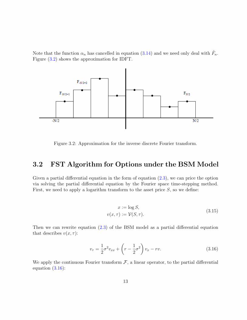
Note that the function αn has cancelled in equation (3.14) and we need only deal with Fn.Figure (3.2) shows the approximation for IDFT.

Figure 3.2: Approximation for the inverse discrete Fourier transform.

3.2 FST Algorithm for Options under the BSM Model

Given a partial differential equation in the form of equation (2.3), we can price the optionvia solving the partial differential equation by the Fourier space time-stepping method.First, we need to apply a logarithm transform to the asset price S, so we define:

x := logS,

v(x, τ) := V(S, τ).(3.15)

Then we can rewrite equation (2.3) of the BSM model as a partial differential equationthat describes v(x, τ):

vτ =1

2σ2vxx +

(r − 1

2σ2

)vx − rv. (3.16)

We apply the continuous Fourier transform F , a linear operator, to the partial differentialequation (3.16):

13

F [vτ ] (k) = F[

1

2σ2vxx

](k) + F

[(r − 1

2σ2

)vx

](k)−F [rv] (k), (3.17)

where the transform variable k represents the frequency. By applying properties of theFourier transform (3.3) and (3.4), we can simplify equation (3.17) as following:

∂

∂τF [v] (k) =

1

2σ2(2πik)2F [v] (k) +

(r − 1

2σ2

)(2πik)F [v] (k)− rF [v] (k). (3.18)

To simplify equation (3.18), we define:

V (k) := F [v] (k). (3.19)

Then equation (3.18) can be written as:

Vτ (k) = Ψ(k) · V (k), (3.20)

where the function Ψ(k) is defined by:

Ψ(k) :=1

2σ2(2πik)2 +

(r − 1

2σ2

)(2πik)− r. (3.21)

Note that the function Ψ(k) is called the characteristic exponent. If we use a linear operatorL to represent the right hand side of equation (3.16) as:

Lv =1

2σ2vxx +

(r − 1

2σ2

)vx − rv, (3.22)

then Ψ(k) can be defined by:

F [Lv](k) = Ψ(k) · V (k). (3.23)

Hence, by applying the Fourier transform and some of its properties, we can convert thepartial differential equation (3.16) in real space into an ordinary differential equation (3.20)in Fourier space. For the BSM model (2.3), the ordinary differential equation (3.20) canbe solved analytically:

14

V (k, τ + ∆τ) = e∆τ ·Ψ(k) · V (k, τ). (3.24)

Here we use the notation V (k, τ + ∆τ) for the value in Fourier space at time τ + ∆τ . Thenthe CFT of v(x, τ) can be approximated by DFT as:

F [v(x, τ)](k) ≈ αn · V (kn, τ)

= αn ·DFT [v(xm, τ)],(3.25)

where:

xm = xmin +m

xmax − xmin

; (m = 0, 1, · · · , N − 1),

kn =n

xmax − xmin

;

(n = −N

2+ 1, · · · , N

2

).

(3.26)

Hence the discrete form of equation (3.24) is:

v(xm, τ + ∆τ) = IDFT [α−1n · V (kn, τ + ∆τ)]

= IDFT [α−1n · e∆τ ·Ψ(n

x) · αn ·DFT [v(xm, τ)]]

= IDFT [e∆τ ·Ψ(nx

) ·DFT [v(xm, τ)]]

= IDFT [e∆τ ·Ψ(kn) ·DFT [v(xm, τ)]].

(3.27)

Note by convention, when we carry out the DFT [v(xm, τ)], (m = 0, 1, · · · , N − 1), thealgorithm generates:

V (kn, τ) ; (n = 0, 1, · · · , N − 1), (3.28)

where:

kn = 0,1

x, · · · ,

N2

x,−N

2+ 1

x, · · · , −1

x. (3.29)

Hence, to form:

15

e∆τ ·Ψ(kn)V (kn, τ) ; (n = 0, 1, · · · , N − 1), (3.30)

one is actually doing:

e∆τ ·Ψ(k′n)V (k′n, τ) ; (n = 0, 1, · · · , N − 1), (3.31)

where V (k′0, τ), V (k′1, τ), · · · , V (k′N−1, τ) are the output of the DFT and where:

k′n =

{nx; n = 0, · · · , N

2,

n−Nx

; n = N2

+ 1, · · · , N − 1.(3.32)

Hence, for a single asset European option under the BSM model, since the ODE can besolved analytically, the option value can be obtained within one timestep. We first applythe Fourier transform, then solve the ODE in Fourier space, and then apply the inverseFourier transform to convert the solution into real space. As for American options, weneed to divide the total time into several time intervals, apply the FST method for onetimestep, add optimal exercise conditions and move to the next timestep.

3.2.1 Fully Implicit and Crank-Nicolson

In order to extend the FST method to commodity models, we will approximate the timederivative by the values in two timesteps. Recall the partial differential equation thatdescribes v(x, τ) under the BSM model:

vτ =1

2σ2vxx +

(r − 1

2σ2

)vx − rv. (3.33)

To simplify, we use a linear operator L to represent the right side:

Lv :=1

2σ2vxx +

(r − 1

2σ2

)vx − rv. (3.34)

Then we use the fully implicit scheme to approximate the derivative vτ as:

[vτ ]n+1i =

vn+1i − vni

∆τ= [Lv]n+1

i . (3.35)

16

We then apply the Fourier transform to equation (3.35) and get:

V n+1(k)− V n(k)

∆τ= Ψ(k) · V n+1(k). (3.36)

Here we use the notation V n(k) for the value in Fourier space at timestep τ = τn. Notehere Ψ(k) is the characteristic exponent defined the term L i.e. F [Lv](k) = Ψ(k) · V (k).Hence, the value at the next timestep vn+1(x) can be expressed as:

vn+1(x) = F−1

[F [vn(x)]

1−∆τ ·Ψ(k)

]. (3.37)

Since the fully implicit is a scheme of first order convergence in time, we can also usethe Crank-Nicolson scheme to obtain second order convergence. Here we approximate thederivative vτ as:

[vτ ]n+1i =

vn+1i − vni

∆τ=

1

2

([Lv]n+1

i + [Lv]ni). (3.38)

Following the same process as the fully implicit scheme, we apply the Fourier transform toequation (3.38):

V n+1(k)− V n(k)

∆τ=

1

2

[Ψ(k) · V n+1(k) + Ψ(k) · V n(k)

]. (3.39)

Hence, the value at the next timestep vn+1(x) can be expressed as:

vn+1(x) = F−1

[F [vn(x)] · (2 + ∆τ ·Ψ(k))

2−∆τ ·Ψ(k)

]. (3.40)

Note that to obtain second order convergence for Crank-Nicolson, we need to apply fullyimplicit for the first two timesteps. This is known as Rannacher smoothing [10]. Algorithms(1) and (2) show the processes of using the FST method with the the fully implicit andCrank-Nicolson methods to price a single asset option under the BSM model.

17

Algorithm 1: FST with fully implicit for single asset option under BSM model.

Data: S,K, r, T, σ,N,mResult: Vx← (xmin, xmin + xmax−xmin

N, · · · , xmin + (N − 1)xmax−xmin

N);

k← 1xmax−xmin

· (0, 1, · · · , N2,−N

2+ 1, · · · ,−1);

p← max(S · exp(x)−K, 0) (call); max(K − S · exp(x), 0) (put);for j ← 1 to N do

Ψj ← 12σ2(2πikj)

2 +(r − 1

2σ2)

(2πikj)− r;end∆τ ← T/m; v← p;for t← 1 to m do

v← DFT [v];for j ← 1 to N do

vj ← vj/(1−∆τ ·Ψj);endv← IDFT [v];if American option then

v← max(v,p);end

endV ← interpolation result of v at x = 0;

18

Algorithm 2: FST with Crank-Nicolson for single asset option under BSM model.

Data: S,K, r, T, σ,N,mResult: Vx← (xmin, xmin + xmax−xmin


N);

k← 1xmax−xmin

· (0, 1, · · · , N2,−N

2+ 1, · · · ,−1);



2 +(r − 1

2σ2)

(2πikj)− r;end∆τ ← T/m; v← p;for t← 1 to 2 do



v← max(v,p);end

endfor t← 3 to m do


vj ← vj · (2 + ∆τ ·Ψj)/(2−∆τ ·Ψj);endv← IDFT [v];if American option then

v← max(v,p);end


3.2.2 FST for European Option under the BSM Model

For a European option with parameters in Table (3.1), the FST method with fully implicitgives first order convergence, given by the results in Table (3.2). As for Crank-Nicolson

19

with Rannacher smoothing, Table (3.3) shows second order convergence. Both are expectedsince fully implicit is a first order method while Crank-Nicolson is a second order method.

Parameter ValueS 100.0K 100.0r 0.1T 1.0σ 0.2

Table 3.1: Single asset option parameters under BSM model.

Nodes Timesteps Value Change Ratio1 Time(s)1024 16 3.71934495 0.00052048 32 3.73481358 -0.01546863 0.00384096 64 3.74373391 -0.00892033 1.73 0.01498192 128 3.74848185 -0.00474794 1.88 0.071716384 256 3.75092669 -0.00244485 1.94 0.2269

Table 3.2: Single asset European put under BSM model, FST with fully implicit, closedform solution = 3.75341839, first order convergence, including both space and time errors.

Nodes Timesteps Value Change Ratio Time(s)1024 16 3.75548948 0.00052048 32 3.75390429 0.00158519 0.00384096 64 3.75353537 0.00036892 4.30 0.01518192 128 3.75344703 0.00008833 4.18 0.074216384 256 3.75342547 0.00002156 4.10 0.2227

Table 3.3: Single asset European put under BSM model, FST with Crank-Nicolson, closedform solution = 3.75341839, second order convergence, including both space and timeerrors.

1If we denote values as V1, V2, · · · , V5, then changes are defined as V1 − V2, · · · , V4 − V5, and ratios aredefined as V1−V2

V2−V3, · · · , V3−V4

V4−V5. The binary logarithm of a ratio shows the order of convergence. That is, a

ratio of 2 corresponds to first order convergence and a ratio of 4 shows second order convergence.

20

3.2.3 FST for American Option under the BSM Model

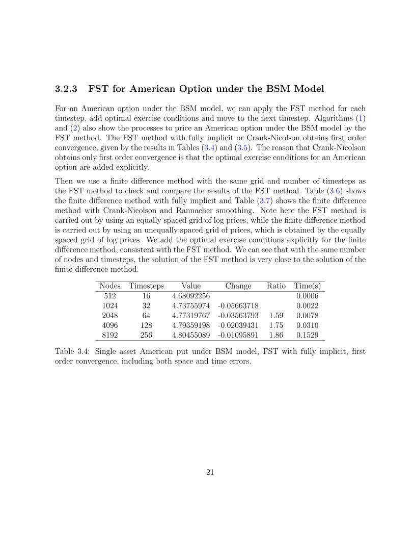
For an American option under the BSM model, we can apply the FST method for eachtimestep, add optimal exercise conditions and move to the next timestep. Algorithms (1)and (2) also show the processes to price an American option under the BSM model by theFST method. The FST method with fully implicit or Crank-Nicolson obtains first orderconvergence, given by the results in Tables (3.4) and (3.5). The reason that Crank-Nicolsonobtains only first order convergence is that the optimal exercise conditions for an Americanoption are added explicitly.

Then we use a finite difference method with the same grid and number of timesteps asthe FST method to check and compare the results of the FST method. Table (3.6) showsthe finite difference method with fully implicit and Table (3.7) shows the finite differencemethod with Crank-Nicolson and Rannacher smoothing. Note here the FST method iscarried out by using an equally spaced grid of log prices, while the finite difference methodis carried out by using an unequally spaced grid of prices, which is obtained by the equallyspaced grid of log prices. We add the optimal exercise conditions explicitly for the finitedifference method, consistent with the FST method. We can see that with the same numberof nodes and timesteps, the solution of the FST method is very close to the solution of thefinite difference method.

Nodes Timesteps Value Change Ratio Time(s)512 16 4.68092256 0.00061024 32 4.73755974 -0.05663718 0.00222048 64 4.77319767 -0.03563793 1.59 0.00784096 128 4.79359198 -0.02039431 1.75 0.03108192 256 4.80455089 -0.01095891 1.86 0.1529

Table 3.4: Single asset American put under BSM model, FST with fully implicit, firstorder convergence, including both space and time errors.

21


Table 3.5: Single asset American put under BSM model, FST with Crank-Nicolson, firstorder convergence, including both space and time errors.

Nodes Timesteps Value Change Ratio Time(s)2

512 16 4.66630596 0.121024 32 4.73376737 -0.06746140 0.812048 64 4.77221789 -0.03845052 1.75 8.574096 128 4.79334001 -0.02112212 1.82 84.028192 256 4.80448634 -0.01114634 1.89 865.62

Table 3.6: Single asset American put under BSM model, finite difference with fully implicit(not vectorized), first order convergence, including both space and time errors.


Table 3.7: Single asset American put under BSM model, finite difference with Crank-Nicolson (not vectorized), first order convergence, including both space and time errors.

2Note that the code for the finite difference method has not been vectorized. Since a vectorized codehas better performance in CPU time, it is not reliable to use CPU time to compare the finite differencemethod with the FST method.

22

Chapter 4

Semi-Lagrangian Method

When we try to use the FST method to solve a partial differential equation derived fromthe commodity one-factor or two-factor model, we cannot obtain an ordinary differentialequation in Fourier space by directly applying the Fourier transform. This is due to thenon-constant velocity term in the partial differential equation. Hence, we consider to usethe semi-Lagrangian method to deal with this problem. The semi-Lagrangian method isa numerical technique for solving partial differential equations describing the advection-diffusion processes.

4.1 Advection-diffusion Equation with Constant Ve-

locity

To introduce the semi-Lagrangian method in a simple context, let us consider a one-dimensional linear advection-diffusion equation of v(x, τ) with a constant coefficient µ:

∂v

∂τ+ µ · ∂v

∂x= 0, (4.1)

with a known initial condition at timestep τ = τ 0:

v(x, τ 0) = v0(x). (4.2)

By solving equation (4.1) using the method of characteristics, we will have the followingsolution:

23

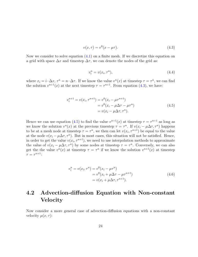
v(x, τ) = v0(x− µτ). (4.3)

Now we consider to solve equation (4.1) on a finite mesh. If we discretize this equation ona grid with space ∆x and timestep ∆τ , we can denote the nodes of the grid as:

vni = v(xi, τn), (4.4)

where xi = i ·∆x, τn = n ·∆τ . If we know the value vn(x) at timestep τ = τn, we can findthe solution vn+1(x) at the next timestep τ = τn+1. From equation (4.3), we have:

vn+1i = v(xi, τ

n+1) = v0(xi − µτn+1)

= v0(xi − µ∆τ − µτn)

= v(xi − µ∆τ, τn).

(4.5)

Hence we can use equation (4.5) to find the value vn+1(x) at timestep τ = τn+1 as long aswe know the solution vn(x) at the previous timestep τ = τn. If v(xi − µ∆τ, τn) happensto be at a mesh node at timestep τ = τn, we then can let v(xi, τ

n+1) be equal to the valueat the node v(xi− µ∆τ, τn). But in most cases, this situation will not be satisfied. Hence,in order to get the value v(xi, τ

n+1), we need to use interpolation methods to approximatethe value of v(xi − µ∆τ, τn) by some nodes at timestep τ = τn. Conversely, we can alsoget the the value vn(x) at timestep τ = τn if we know the solution vn+1(x) at timestepτ = τn+1:

vni = v(xi, τn) = v0(xi − µτn)

= v0(xi + µ∆τ − µτn+1)

= v(xi + µ∆τ, τn+1).

(4.6)

4.2 Advection-diffusion Equation with Non-constant

Velocity

Now consider a more general case of advection-diffusion equations with a non-constantvelocity µ(x, τ):

24

∂v

∂τ+ µ(x, τ) · ∂v

∂x= 0, (4.7)

with a known initial condition at timestep τ = τ 0:

v(x, τ 0) = v0(x). (4.8)

To solve equation (4.7) using the method of characteristics, we first need to define a functionX(x, s; τ), s ∈ [0, T ] to be the solution to the following ordinary differential equation:

D

DτX(x, s; τ) = µ(X(x, s; τ), τ),

X(x, s; s) = x.(4.9)

Then we consider the Lagrangian derivative DDτv(X(x, s; τ), τ), which describes the rate

of change in time of v subjected to a space-and-time-dependent velocity field X(x, s; τ).With the chain rule, we have:

D

Dτv(X(x, s; τ), τ) =

[∂

∂τ+

D

DτX(x, s; τ) · ∂

∂x

]v(X(x, s; τ), τ)

=

[∂

∂τ+ µ(X(x, s; τ), τ) · ∂

∂x

]v(X(x, s; τ), τ)

= 0,

(4.10)

and we have:

v(X(x, s; τ), τ) = constant. (4.11)

In order to use this for numerical computations, we need to solve equation (4.7) on a finitegrid. Thus for the value at timestep τ = τn+1, we first define a function X(x, τn+1; τ) tobe the solution to the following ODE:

D

DτX(x, τn+1; τ) = µ(X(x, τn+1; τ), τ),

X(x, τn+1; τn+1) = x.(4.12)

25

Figure 4.1: Semi-Lagrangian scheme.

By the above discussion, we know v(X(x, τn+1; τ), τ) = constant, we have:

v(xi, τn+1) = v(X(xi, τ

n+1; τn+1), τn+1)

= v(X(xi, τn+1; τn), τn).

(4.13)

Following the same process, for the value at timestep τ = τn, we also have:

v(xi, τn) = v(X(xi, τ

n; τn), τn)

= v(X(xi, τn; τn+1), τn+1).

(4.14)

Figure (4.1) shows the characteristic curve of the semi-Lagrangian scheme. We can useequation (4.13) to find the value vn+1(x) at timestep τ = τn+1 as long as we know the

26

solution vn(x) at timestep τ = τn. Hence, for each timestep τ = τn, we first solve theordinary differential equation (4.9) to determine the value of X(xi, τ

n+1; τn). Then we useinterpolation methods to approximate this value by some nodes at timestep τ = τn. Theresult will be the solution v(xi, τ

n+1) at timestep τ = τn+1.

4.3 Application to the Commodity Price Models

Since some commodity price models, including one-factor and two-factor models, havestochastic drift terms, the partial differential equations for pricing commodity-based op-tions will typically be advection-diffusion equations. We can apply the semi-Lagrangianmethod to deal with the stochastic drift term, which will be the non-constant velocityterm in the advection-diffusion equation. After that, it is convenient to use the Fourierspace time-stepping method to obtain the value of the option. Suppose we need to pricean option v(x, τ) with the pricing partial differential equation:

Dv

Dτ=∂v

∂τ+ µ(x, τ) · ∂v

∂x= Lv, (4.15)

where the notation Dv/Dτ is for the Lagrangian derivative, and L is a linear operator forthe rest terms of the partial differential equation. To apply the semi-Lagrangian method,we first define a function X(x, s; τ) to be the solution to the ordinary differential equation(4.9). Then we use the fully implicit method to deal with the Lagrangian derivative Dv/Dτby:

[Dv

Dτ

]n+1

i

=vn+1i − vni∗

∆τ= [Lv]n+1

i . (4.16)

From the semi-Lagrangian discussion above, we can use equation (4.14)

vni∗ = v(xi∗ , τn) = v(X(xi∗ , τ

n; τn+1), τn+1),

to rewrite equation (4.16) as:

vn+1i − v(X(xi∗ , τ

n; τn+1), τn+1)

∆τ= [Lv]n+1

i . (4.17)

To apply the Fourier space time-stepping method, we first define the Fourier transform ofv(X(xi∗ , τ

n; τn+1), τn+1) as:

27

V n(k) := F[v(X(xi∗ , τ

n; τn+1), τn+1)]

(k). (4.18)

We apply the Fourier transform to equation (4.17) and obtain the following equation:

V n+1(k)− V n(k)

∆τ= Ψ(k) · V n+1(k), (4.19)

where Ψ(k) is the characteristic exponent defined the term L, i.e. F [Lv](k) = Ψ(k) ·V (k).Finally, by simplifying equation (4.19), we have:

V n+1(k) =V n(k)

1−∆τ ·Ψ(k). (4.20)

Since the value v(X(xi∗ , τn; τn+1), τn+1) at timestep τ = τn+1 can be approximated by the

value vn(x) at timestep τ = τn via interpolation methods, we can use the following processto solve the value at the next timestep:

vn(x)interpolation−−−−−−−→ v(X(xi∗ , τ

n; τn+1), τn+1)DFT−−−→ V n(k)

(4.20)−−−→ V n+1(k)IDFT−−−→ vn+1(x).

(4.21)

Moreover, we can also use the Crank-Nicolson method to deal with the Lagrangian deriva-tive Dv/Dτ , then instead of equation (4.16), we have:

[Dv

Dτ

]n+1

i

=vn+1i − vni∗

∆τ=

1

2

([Lv]n+1

i + [Lv]ni∗). (4.22)

From the semi-Lagrangian discussion above, we can use equation (4.14)

vni∗ = v(xi∗ , τn) = v(X(xi∗ , τ

n; τn+1), τn+1),

to rewrite equation (4.22) as:

vn+1i − v(X(xi∗ , τ

n; τn+1), τn+1)

∆τ=

1

2

([Lv]n+1

i + [Lv]ni∗). (4.23)

For the term [Lv]ni∗ , we need to first apply L to get the value of [Lv]ni , and then do aninterpolation step to get the value of [Lv]ni∗ . Also, we define:

28

V n(k) := F[v(X(xi∗ , τ

n; τn+1), τn+1)]

(k),

LV n(k) := F [[Lv]ni∗ ] (k).(4.24)

Note here [Lv]ni∗ is obtained by:

[Lv]ni∗ = interpolation result of F−1[Ψ(k) · F [vni ](k)] at X(xi∗ , τn; τn+1). (4.25)

By the above definition, we apply the Fourier transform to equation (4.23) and get thefollowing equation:

V n+1(k)− V n(k)

∆τ=

1

2

[Ψ(k) · V n+1(k) + LV n(k)

]. (4.26)

Hence, following the similar derivation as before, we have:

V n+1(k) =2 · V n(k) + ∆τ · LV n(k)

2−∆τ ·Ψ(k). (4.27)

Instead of equation (4.20) for the fully implicit method, we can use equation (4.27) of theCrank-Nicolson method to do the Fourier space time-stepping process. In the implemen-tation of Crank-Nicolson, we need to do the first two timesteps as fully implicit, known asRannacher smoothing [10]. This gives us second order convergence for Crank-Nicolson.

4.4 Interpolation Methods

Interpolation is a numerical method of constructing new data points within the range of adiscrete set of known data points. One of the simplest methods is linear interpolation. Theinterpolated value of the point that does not lie on any existing grid points is determinedby the two neighbouring grid points in each respective dimension. Given two grid points(x0, y0) and (x1, y1), where we assume x0 6= x1, we can perform a straight line (first orderpolynomial) between the two points. Then the value of an interpolated point (x, y) between(x0, y0) and (x1, y1) is given by:

29

y = y0 + (x− x0) · y1 − y0

x1 − x0

. (4.28)

The method of linear interpolation is very straightforward and easy to implement. Butits disadvantages are obvious. Given N data points (xi, yi) where i = 0, 1, · · · , N − 1, ifh = maxN−1

i=1 (xi − xi−1), the error of linear interpolation is O(h2). For the interpolation ina two-dimensional space, we perform linear interpolation first in one direction, and thenagain in the other direction. This interpolation can be used in the FST method for atwo-factor model.

Figure 4.2: Linear interpolation and piecewise quadratic interpolation.

To get a more accurate interpolation result, we can extend linear interpolation to morethan two data points. A typical second order interpolation method is piecewise quadraticinterpolation. We first divide all the intervals into several pairs with each pair having twoclosed intervals. Then for the three points in each pair of intervals, we construct a quadratic

30

Lagrange polynomial. So the global interpolant will be a piecewise quadratic polynomial.Given N data points (xi, yi) where i = 0, 1, · · · , N − 1, if h = maxN−1

i=1 (xi−xi−1), the errorof piecewise quadratic interpolation is O(h3). Figure (4.2) shows the linear and piecewisequadratic interpolations for a typical function. Another possibility, which forces moresmoothness of the interpolant, is to use a piecewise cubic spline, with local error O(h4).However, a cubic spline forces continuity of the second derivatives. This property does nothold for an American option.

4.5 Error of the Semi-Lagrangian Method

We assume ∆x = O(∆τ) = O(h) and the local interpolation error is O(hq). We alsoassume the global time-stepping error is O(hp), where p = 1 for fully implicit, and p = 2for Crank-Nicolson. The space discretization error is O(h2) due to the trapezoidal ruleequation (3.10). Hence, the final result of the global error for the FST time-stepping withthe semi-Lagrangian method is given by:

global error = O

(hq

∆τ

)+O(hp) +O(h2)

= O(hq−1) +O(hp) +O(h2).

(4.29)

From equation (4.29), we can see that we need to use an interpolation method with q ≥ 3in order to get second order convergence with Crank-Nicolson, i.e. the piecewise quadraticor higher order interpolation method.

31

Chapter 5

Numerical Results

5.1 Commodity Options under a One-factor Model

5.1.1 FST Algorithm for Options under a One-factor Model

Under the commodity price one-factor model, we have the options pricing partial differen-tial equation (2.8) that describes V(S, τ):

Vτ =1

2σ2S2VSS + κ(µ− λ− logS)SVS. (5.1)

In order to solve the partial differential equation (5.1) by the Fourier space time-steppingmethod, we first need to apply a logarithm transform to the asset price S. Thus we define:

x := logS,

v(x, τ) := V(S, τ),(5.2)

and rewrite equation (5.1) as a partial differential equation describing v(x, τ):

vτ =1

2σ2vxx +

[κ(µ− λ− x)− 1

2σ2

]vx. (5.3)

To simplify, we define:

32

a− bx := κ(µ− λ− x)− 1

2σ2, (5.4)

with the values of a and b being:

a = κ(µ− λ)− 1

2σ2,

b = κ.(5.5)

To solve equation (5.3) using the method of characteristics, we first need to define a functionX(x, s; τ) to be the solution to the following ordinary differential equation:

D

DsX(x, s; τ) = µ(X(x, s; τ), τ),

X(x, s; s) = x,(5.6)

where:

µ(x, τ) = bx− a. (5.7)

It is easy to get this solution as:

X(x, s; τ) = xeb(s−τ) − a

b

(eb(s−τ) − 1

). (5.8)

If we rewrite equation (5.3) as:

Dv

Dτ= Lv, (5.9)

where Lv is given by:

Lv =1

2σ2vxx, (5.10)

then we can apply the semi-Lagrangian method. Here the characteristic exponent Ψ(k) isdefined by the term Lv and given by:

33

Ψ(k) :=1

2σ2(2πik)2. (5.11)

Algorithms (3) and (4) show the processes of using the FST method with fully implicitand Crank-Nicolson to price a single asset option under a one-factor model.

Algorithm 3: FST with fully implicit for single asset commodity option under one-factor model.

Data: S,K, µ, T, σ, κ, λ,N,mResult: Vx← (xmin, xmin + xmax−xmin


N);

k← 1xmax−xmin

· (0, 1, · · · , N2,−N

2+ 1, · · · ,−1);



2;end∆τ ← T/m; a← κ(µ− λ)− 1

2σ2; b← κ;

x← x · exp{−b∆τ} − ab· (exp{−b∆τ} − 1); v← p;

for t← 1 to m dov← interpolation result of v at x = x;v← DFT [v];for j ← 1 to N do


v← max(v,p);end


34

Algorithm 4: FST with Crank-Nicolson for single asset commodity option underone-factor model.

Data: S,K, µ, T, σ, κ, λ,N,mResult: Vx← (xmin, xmin + xmax−xmin


N);

k← 1xmax−xmin

· (0, 1, · · · , N2,−N

2+ 1, · · · ,−1);



2;end∆τ ← T/m; a← κ(µ− λ)− 1

2σ2; b← κ;

x← x · exp{−b∆τ} − ab· (exp{−b∆τ} − 1); v← p;

for t← 1 to 2 dov← interpolation result of v at x = x;v← DFT [v];for j ← 1 to N do


v← max(v,p);end



Lj ← vj ·Ψj;endL← IDFT [L];L← interpolation result of L at x = x; v← interpolation result of v at x = x;L← DFT [L]; v← DFT [v];for j ← 1 to N do

vj ← (2 · vj + ∆τ · Lj)/(2−∆τ ·Ψj);endv← IDFT [v];if American option then

v← max(v,p);end

endV ← interpolation result of v at x = 0; 35

5.1.2 Monte Carlo for European Option under a One-factor Model

To check the results of our algorithms, we first use Monte Carlo simulations to price aEuropean call under a one-factor model. Table (5.1) shows parameters of the option undera one-factor model. The option values with standard errors of Monte Carlo simulationsare listed in Table (5.2).

Parameter ValueS 100.0K 100.0µ 0.1T 1.0σ 0.1κ 0.1λ 0.2

Table 5.1: Single asset commodity option parameters under one-factor model.

Simulations Timesteps Value StdError Ratio Time(s)100000 1000 0.87632401 0.01730161 2.41200000 2000 0.87986616 0.01225448 1.41 10.78400000 4000 0.88295630 0.00874660 1.40 42.97800000 8000 0.87461189 0.00612923 1.43 171.571600000 16000 0.87940762 0.00435362 1.41 700.92

Table 5.2: Single asset commodity European call under one-factor model, Monte Carlo.

5.1.3 FST for European Option under a One-factor Model

As shown in Tables (5.3), (5.4) and (5.5), for a European option, the fully implicit time-stepping results in first order convergence for linear, piecewise quadratic, and cubic splineinterpolations. Since fully implicit is a first order scheme, higher order interpolation methoddoes not result in higher order convergence, as expected from equation (4.29).

36


Table 5.3: Single asset commodity European call under one-factor model, fully implicit withlinear interpolation, Monte Carlo solution = 0.87940762 (standard error = 0.00435362),first order convergence, including both space and time errors.


Table 5.4: Single asset commodity European call under one-factor model, fully implicitwith piecewise quadratic interpolation (not vectorized), Monte Carlo solution = 0.87940762(standard error = 0.00435362), first order convergence, including both space and timeerrors.


Table 5.5: Single asset commodity European call under one-factor model, fully implicitwith cubic spline interpolation, Monte Carlo solution = 0.87940762 (standard error =0.00435362), first order convergence, including both space and time errors.

37

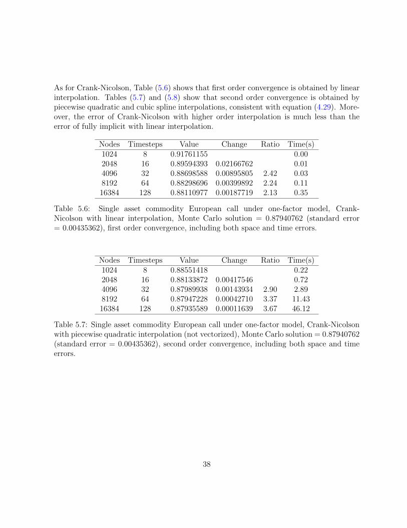
As for Crank-Nicolson, Table (5.6) shows that first order convergence is obtained by linearinterpolation. Tables (5.7) and (5.8) show that second order convergence is obtained bypiecewise quadratic and cubic spline interpolations, consistent with equation (4.29). More-over, the error of Crank-Nicolson with higher order interpolation is much less than theerror of fully implicit with linear interpolation.


Table 5.6: Single asset commodity European call under one-factor model, Crank-Nicolson with linear interpolation, Monte Carlo solution = 0.87940762 (standard error= 0.00435362), first order convergence, including both space and time errors.


Table 5.7: Single asset commodity European call under one-factor model, Crank-Nicolsonwith piecewise quadratic interpolation (not vectorized), Monte Carlo solution = 0.87940762(standard error = 0.00435362), second order convergence, including both space and timeerrors.

38


Table 5.8: Single asset commodity European call under one-factor model, Crank-Nicolsonwith cubic spline interpolation, Monte Carlo solution = 0.87940762 (standard error =0.00435362), second order convergence, including both space and time errors.

39

5.1.4 FST for American Option under a One-factor Model

As shown in Tables (5.9), (5.10) and (5.11), for an American option, fully implicit obtainsfirst order convergence for linear, piecewise quadratic, and cubic spline interpolations.


Table 5.9: Single asset commodity American call under one-factor model, fully implicitwith linear interpolation, first order convergence, including both space and time errors.


Table 5.10: Single asset commodity American call under one-factor model, fully implicitwith piecewise quadratic interpolation (not vectorized), first order convergence, includingboth space and time errors.

40


Table 5.11: Single asset commodity American call under one-factor model, fully implicitwith cubic spline interpolation, first order convergence, including both space and timeerrors.

41

As for Crank-Nicolson, since the optimal exercise conditions are added explicitly, first orderconvergence is obtained for linear, piecewise quadratic, and cubic spline interpolations. Theresults are shown in Tables (5.12), (5.13) and (5.14).


Table 5.12: Single asset commodity American call under one-factor model, Crank-Nicolsonwith linear interpolation, first order convergence, including both space and time errors.


Table 5.13: Single asset commodity American call under one-factor model, Crank-Nicolsonwith piecewise quadratic interpolation (not vectorized), first order convergence, includingboth space and time errors.


Table 5.14: Single asset commodity American call under one-factor model, Crank-Nicolsonwith cubic spline interpolation, first order convergence, including both space and timeerrors.

42

5.2 Commodity Options under a Two-factor Model

5.2.1 FST Algorithm for Options under a Two-factor Model

Under the commodity price two-factor model, we have the options pricing partial differen-tial equation (2.13) that describes V(S, δ, τ):

Vτ =1

2σ2

1S2VSS + σ1σ2ρSVSδ +

1

2σ2

2Vδδ + (r − δ)SVS + κ[(α− δ)− λ]Vδ. (5.12)

In order to solve the partial differential equation (5.12) by the Fourier space time-steppingmethod, we first need to apply a logarithm transform to the asset price S. Thus we define:

x := logS,

v(x, δ, τ) := V(S, δ, τ),(5.13)

and rewrite equation (5.12) as a partial differential equation describing v(x, δ, τ):

vτ =1

2σ2

1vxx + σ1σ2ρvxδ +1

2σ2

2vδδ +

[(r − δ)− 1

2σ2

1

]vx + κ[(α− δ)− λ]vδ. (5.14)

To simplify, we define:

a1 − b1δ := (r − δ)− 1

2σ2

1,

a2 − b2δ := κ[(α− δ)− λ],(5.15)

with the values of a1, b1, a2, b2 being:

a1 = r − 1

2σ2

1,

b1 = 1,

a2 = κ(α− λ),

b2 = κ.

(5.16)

43

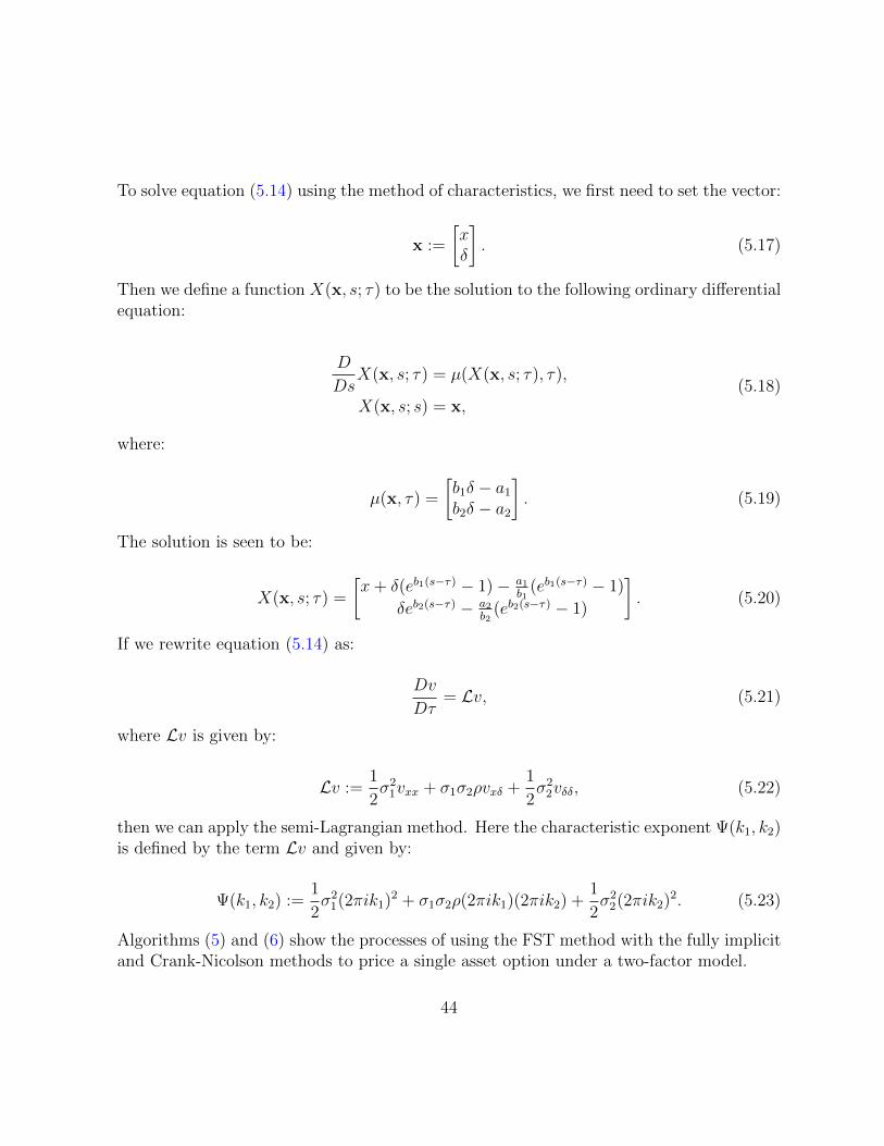
To solve equation (5.14) using the method of characteristics, we first need to set the vector:

x :=

[xδ

]. (5.17)

Then we define a function X(x, s; τ) to be the solution to the following ordinary differentialequation:

D

DsX(x, s; τ) = µ(X(x, s; τ), τ),

X(x, s; s) = x,(5.18)

where:

µ(x, τ) =

[b1δ − a1

b2δ − a2

]. (5.19)

The solution is seen to be:

X(x, s; τ) =

[x+ δ(eb1(s−τ) − 1)− a1

b1(eb1(s−τ) − 1)

δeb2(s−τ) − a2b2

(eb2(s−τ) − 1)

]. (5.20)

If we rewrite equation (5.14) as:

Dv

Dτ= Lv, (5.21)

where Lv is given by:

Lv :=1

2σ2

1vxx + σ1σ2ρvxδ +1

2σ2

2vδδ, (5.22)

then we can apply the semi-Lagrangian method. Here the characteristic exponent Ψ(k1, k2)is defined by the term Lv and given by:

Ψ(k1, k2) :=1

2σ2

1(2πik1)2 + σ1σ2ρ(2πik1)(2πik2) +1

2σ2

2(2πik2)2. (5.23)

Algorithms (5) and (6) show the processes of using the FST method with the fully implicitand Crank-Nicolson methods to price a single asset option under a two-factor model.

44

Algorithm 5: FST with fully implicit for single asset commodity option under two-factor model.

Data: S, δ,K, r, T, σ1, σ2, ρ, κ, α, λ,N,mResult: Vx1,x2← (xmin, xmin + xmax−xmin


N);

k1,k2← 1xmax−xmin

· (0, 1, · · · , N2,−N

2+ 1, · · · ,−1);

for l← 1 to N dopl: ← max(S · exp(x1l)−K, 0) (call); max(K − S · exp(x1l), 0) (put);

endfor l← 1 to N do

for j ← 1 to N doΨlj ← 1

2σ2

1(2πik1l)2 + 1

2σ2

2(2πik2j)2 + σ1σ2ρ(2πik1l)(2πik2j);

end

end∆τ ← T/m; a1 ← r − 1

2σ2

1; b1 ← 1; a2 ← κ(α− λ); b2 ← κ;

x2← x2 · exp{−b2∆τ} − a2b2· (exp{−b2∆τ} − 1); v← p;

for t← 1 to m dofor j ← 1 to N do

x1← x1 + x2j · (exp{−b1∆τ} − 1)− a1b1· (exp{−b1∆τ} − 1);

v:j ← interpolation result of v at x1 = x1, x2 = x2j;endv← DFT [v];for l← 1 to N do

for j ← 1 to N dovlj ← vlj/(1−∆τ ·Ψlj);

end

endv← IDFT [v];if American option then

v← max(v,p);end

endV ← interpolation result of v at x1 = 0, x2 = 0;

45

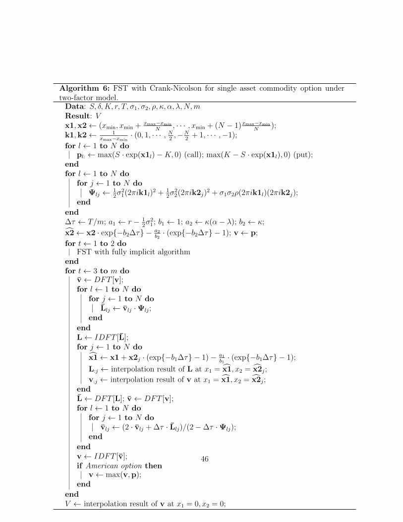
Algorithm 6: FST with Crank-Nicolson for single asset commodity option undertwo-factor model.

Data: S, δ,K, r, T, σ1, σ2, ρ, κ, α, λ,N,mResult: Vx1,x2← (xmin, xmin + xmax−xmin


N);

k1,k2← 1xmax−xmin

· (0, 1, · · · , N2,−N

2+ 1, · · · ,−1);

for l← 1 to N dopl: ← max(S · exp(x1l)−K, 0) (call); max(K − S · exp(x1l), 0) (put);

endfor l← 1 to N do

for j ← 1 to N doΨlj ← 1

2σ2

1(2πik1l)2 + 1

2σ2

2(2πik2j)2 + σ1σ2ρ(2πik1l)(2πik2j);

end

end∆τ ← T/m; a1 ← r − 1

2σ2

1; b1 ← 1; a2 ← κ(α− λ); b2 ← κ;

x2← x2 · exp{−b2∆τ} − a2b2· (exp{−b2∆τ} − 1); v← p;

for t← 1 to 2 doFST with fully implicit algorithm


v← DFT [v];for l← 1 to N do

for j ← 1 to N doLlj ← vlj ·Ψlj;

end

endL← IDFT [L];for j ← 1 to N do

x1← x1 + x2j · (exp{−b1∆τ} − 1)− a1b1· (exp{−b1∆τ} − 1);

L:j ← interpolation result of L at x1 = x1, x2 = x2j;

v:j ← interpolation result of v at x1 = x1, x2 = x2j;endL← DFT [L]; v← DFT [v];for l← 1 to N do

for j ← 1 to N dovlj ← (2 · vlj + ∆τ · Llj)/(2−∆τ ·Ψlj);

end

endv← IDFT [v];if American option then

v← max(v,p);end

endV ← interpolation result of v at x1 = 0, x2 = 0;

46

5.2.2 Monte Carlo for European Option under a Two-factor Model

To check the results of our algorithms, we first use Monte Carlo simulations to price aEuropean put under a two-factor model. Table (5.15) shows parameters of the option undera two-factor model. The option values with standard errors of Monte Carlo simulationsare listed in Table (5.16).

Parameter ValueS 100.0δ 100.0K 100.0r 0.1T 1.0σ1 0.1σ2 0.2ρ 0.5κ 0.1α 0.1λ 0.2

Table 5.15: Single asset commodity option parameters under two-factor model.

Simulations Timesteps Value StdError Ratio Time(s)100000 1000 1.10924986 0.01914251 6.19200000 2000 1.09865181 0.01349634 1.42 21.31400000 4000 1.10506938 0.00956445 1.41 89.26800000 8000 1.10213963 0.00673322 1.42 353.961600000 16000 1.10497142 0.00477254 1.41 1509.14

Table 5.16: Single asset commodity European put under two-factor model, Monte Carlo.

5.2.3 FST for European Option under a Two-factor Model

As shown in Tables (5.17), (5.18) and (5.19), for a European option, fully implicit obtainsfirst order convergence for linear, piecewise quadratic, and cubic spline interpolations. Since

47

fully implicit is a first order scheme, only first order convergence is obtained, regardless ofthe interpolation methods.

Nodes Timesteps Value Change Ratio Time(s)2562 8 1.82624602 0.855122 16 1.42184384 0.40440219 3.6210242 32 1.25043458 0.17140926 2.36 17.1520482 64 1.17387687 0.07655771 2.24 94.05

Table 5.17: Single asset commodity European put under two-factor model, fully im-plicit with linear interpolation, Monte Carlo solution = 1.10497142 (standard error =0.00477254), first order convergence, including both space and time errors.


Table 5.18: Single asset commodity European put under two-factor model, fully implicitwith piecewise quadratic interpolation (not vectorized), Monte Carlo solution = 1.10497142(standard error = 0.00477254), first order convergence, including both space and timeerrors.


Table 5.19: Single asset commodity European put under two-factor model, fully implicitwith cubic spline interpolation, Monte Carlo solution = 1.10497142 (standard error =0.00477254), first order convergence, including both space and time errors.

48

As for Crank-Nicolson, Table (5.20) shows that first order convergence is obtained by linearinterpolation. Tables (5.21) and (5.22) show that second order convergence is obtainedby piecewise quadratic and cubic spline interpolations, consistent with equation (4.29).Moreover, the error of Crank-Nicolson with higher order interpolation is much less thanthe error of fully implicit with linear interpolation.


Table 5.20: Single asset commodity European put under two-factor model, Crank-Nicolson with linear interpolation, Monte Carlo solution = 1.10497142 (standard error= 0.00477254), first order convergence, including both space and time errors.


Table 5.21: Single asset commodity European put under two-factor model, Crank-Nicolsonwith piecewise quadratic interpolation (not vectorized), Monte Carlo solution = 1.10497142(standard error = 0.00477254), second order convergence, including both space and timeerrors.

49


Table 5.22: Single asset commodity European put under two-factor model, Crank-Nicolsonwith cubic spline interpolation, Monte Carlo solution = 1.10497142 (standard error =0.00477254), second order convergence, including both space and time errors.

50

5.2.4 FST for American Option under a Two-factor Model

As shown in Tables (5.23), (5.24) and (5.25), for an American option, fully implicit obtainsfirst order convergence for linear, piecewise quadratic, and cubic spline interpolations.

Nodes Timesteps Value Change Ratio Time(s)10242 8 2.03947509 4.1820482 16 2.12046638 -0.08099130 22.9540962 32 2.16632205 -0.04585567 1.77 140.3181922 64 2.18831556 -0.02199351 2.08 890.93

Table 5.23: Single asset commodity American put under two-factor model, fully implicitwith linear interpolation, first order convergence, including both space and time errors.


Table 5.24: Single asset commodity American put under two-factor model, fully implicitwith piecewise quadratic interpolation (not vectorized), first order convergence, includingboth space and time errors.


Table 5.25: Single asset commodity American put under two-factor model, fully implicitwith cubic spline interpolation, first order convergence, including both space and timeerrors.

51

As for Crank-Nicolson, since the optimal exercise conditions are added explicitly, first orderconvergence is obtained for linear, piecewise quadratic, and cubic spline interpolations. Theresults are shown in Tables (5.26), (5.27) and (5.28).


Table 5.26: Single asset commodity American put under two-factor model, Crank-Nicolsonwith linear interpolation, first order convergence, including both space and time errors.


Table 5.27: Single asset commodity American put under two-factor model, Crank-Nicolsonwith piecewise quadratic interpolation (not vectorized), first order convergence, includingboth space and time errors.


Table 5.28: Single asset commodity American put under two-factor model, Crank-Nicolsonwith cubic spline interpolation, first order convergence, including both space and timeerrors.

52

Chapter 6

Conclusions

In this paper, we present the framework for pricing contingent claims by the Fourier spacetime-stepping method. The pricing partial differential equation can be converted to anordinary differential equation in Fourier space. Then the time-stepping can be completedin one timestep between discrete monitoring dates where constraints and conditions areapplied. Since the ordinary differential equation can be solved accurately and efficiently inFourier space, this method can be seen as an useful method for pricing contingent claims,especially for path-dependent options like American and some types of Asian options.

Furthermore, we also extend the Fourier space time-stepping method to some mean-reverting models, which are widely used in commodity prices. The semi-Lagrangian methodcan be used to deal with the stochastic drift terms in the pricing partial differential equa-tions of the commodity one-factor and two-factor models. We simply need to add aninterpolation step in the Fourier space time-stepping method, which gives us quite rea-sonable results for commodity European and American options. For European options,first order convergence is obtained by fully implicit with linear, piecewise quadratic, andcubic spline interpolations. As for Crank-Nicolson with Rannacher smoothing, linear in-terpolation gives us first order convergence while piecewise quadratic and cubic splineinterpolations give us second order convergence. For American options, as the optimalexercise conditions are added explicitly, for both fully implicit and Crank-Nicolson, firstorder convergence is obtained.

As discussed in this paper, further research can include

• Use a second order backward differentiation formula (BDF) to approximate the time

53

derivative.

• Extend the Fourier space time-stepping method to other types of contingent claimsin commodity markets.

• Use graphics processing units (GPUs) to speed up the computational processes ofthe fast Fourier transform (FFT) and the inverse fast Fourier transform (IFFT).

• Use graphics processing units (GPUs) to speed up the interpolation operations.

54

APPENDICES

55

Appendix A

Wrap-around Error

In the computation of the Fourier space time-stepping method, the Fourier transform as-sumes a periodic domain implicitly, while the real domain of the log asset price is aperiodic.Consequently, when the Fourier transform is applied, it causes values at the end of the gridto be ”wrapped around” to the other side of the grid. The values near the far right endof the domain, the log asset prices x close to xmax, will wrap around and produce wrongsolutions at the left end of the grid, similarly with the asset prices close to xmin.

A simple method to reduce the wrap-around error is to use zero padding. For the domainin real space, we add zeros and the DFT operation is done on a grid with the size twiceas the original length. And for the domain in Fourier space, the number of nodes is alsodoubled. Then during the FST process, after applying the inverse Fourier transform, theadded zero value nodes are deleted. If one just tries to solve an option price with an initialasset price S, one can use this S as the centre of the grid. Then the wrap-around error willnot occur. However, if one tries to solve problems with several initial asset prices at onetime, the warp-around error will occur when an initial asset price S is near the end of thegrid. In this case, one can set the centre of the grid as the mean value of the maximuminitial asset price and the minimum initial asset price. Then with zero padding, all theproblems should have reasonable results. Algorithm (7) shows the process to apply zeropadding for the FST method. Note that the grid in Algorithm (7) is centred at Sc.

With the option parameters shown in Table (A.1), Table (A.2) shows the solutions of theFST method with and without zero padding. Note that the grid here is centred (in thelog asset price domain) at Sc = 100. The FST solution without zero padding when S = Scis very close to the closed form solution. But for the values near the end of the grid, theFST solutions without zero padding are quite unreasonable while the FST solutions with

56

zero padding still give us results that are close to the closed form solutions.

Algorithm 7: FST with fully implicit for single asset option under BSM model (withzero padding).

Data: S,K, r, T, σ,N,m, ScResult: Vx← (xmin, xmin + xmax−xmin


N);

k← 12·(xmax−xmin)

· (0, 1, · · · , N,−N + 1, · · · ,−1︸︷︷︸2N

);

p′ ← max(Sc · exp(x)−K, 0) (call); max(K − Sc · exp(x), 0) (put);p← (0, · · · , 0︸︷︷︸

N2

, p′︸︷︷︸N

, 0, · · · , 0︸︷︷︸N2

);

for j ← 1 to 2N doΨj ← 1

2σ2(2πikj)

2 +(r − 1

2σ2)

(2πikj)− r;end∆τ ← T/m; v← p;for t← 1 to m do



v← max(v,p);end

endfor j ← 1 to N do

v′j ← vj+N2

;

endV ← interpolation result of v′ at p′ = S;

57

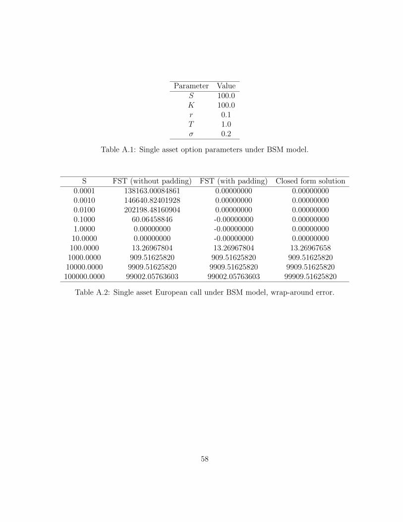
Parameter ValueS 100.0K 100.0r 0.1T 1.0σ 0.2

Table A.1: Single asset option parameters under BSM model.

S FST (without padding) FST (with padding) Closed form solution0.0001 138163.00084861 0.00000000 0.000000000.0010 146640.82401928 0.00000000 0.000000000.0100 202198.48160904 0.00000000 0.000000000.1000 60.06458846 -0.00000000 0.000000001.0000 0.00000000 -0.00000000 0.0000000010.0000 0.00000000 -0.00000000 0.00000000100.0000 13.26967804 13.26967804 13.269676581000.0000 909.51625820 909.51625820 909.5162582010000.0000 9909.51625820 9909.51625820 9909.51625820100000.0000 99002.05763603 99002.05763603 99909.51625820

Table A.2: Single asset European call under BSM model, wrap-around error.

58

References

[1] F. Black and M. Scholes, The pricing of options and corporate liabilities, TheJournal of Political Economy, 81 (1973), pp. 637–654.

[2] Z. Chen and P. A. Forsyth, A semi-Lagrangian approach for natural gas storagevaluation and optimal operation, SIAM Journal on Scientific Computing, 30 (2007),pp. 339–368.

[3] Y. d’Halluin, P. A. Forsyth, and G. Labahn, A semi-Lagrangian approach forAmerican Asian options under jump diffusion, SIAM Journal on Scientific Computing,27 (2005), pp. 315–345.

[4] R. Gibson and E. S. Schwartz, Stochastic convenience yield and the pricing ofoil contingent claims, The Journal of Finance, 45 (1990), pp. 959–976.

[5] T. R. Hurd and Z. Zhou, A Fourier transform method for spread option pricing,SIAM Journal on Financial Mathematics, 1 (2010), pp. 142–157.

[6] K. R. Jackson, S. Jaimungal, and V. Surkov, Fourier space time-steppingfor option pricing with Levy models, Journal of Computational Finance, 12 (2008),pp. 1–28.

[7] S. Jaimungal and V. Surkov, Levy-based cross-commodity models and derivativevaluation, SIAM Journal on Financial Mathematics, 2 (2011), pp. 464–487.

[8] K. R. Miltersen and E. S. Schwartz, Pricing of options on commodity futureswith stochastic term structures of convenience yields and interest rates, Journal ofFinancial and Quantitative Analysis, 33 (1998), pp. 33–59.

[9] D. M. Pooley, K. R. Vetzal, and P. A. Forsyth, Convergence remedies fornon-smooth payoffs in option pricing, Journal of Computational Finance, 6 (2003),pp. 25–40.

59

[10] R. Rannacher, Finite element solution of diffusion problems with irregular data,Numerische Mathematik, 43 (1984), pp. 309–327.

[11] S. A. Ross, Hedging long run commitments: Exercises in incomplete market pricing,Economic Notes, 26 (1997), pp. 385–420.

[12] E. S. Schwartz, The stochastic behavior of commodity prices: Implications for val-uation and hedging, The Journal of Finance, 52 (1997), pp. 923–973.

[13] E. S. Schwartz and J. E. Smith, Short-term variations and long-term dynamicsin commodity prices, Management Science, 46 (2000), pp. 893–911.

[14] A. Staniforth and J. Cote, Semi-Lagrangian integration schemes for atmosphericmodels-a review, Monthly Weather Review, 119 (1991), pp. 2206–2223.

[15] V. Surkov, Option pricing using Fourier space time-stepping framework, PhD thesis,University of Toronto, 2009.

[16] A. Ware, Accurate semi-Lagrangian time stepping for stochastic optimal control prob-lems with application to the valuation of natural gas storage, SIAM Journal on Finan-cial Mathematics, 4 (2013), pp. 427–451.

[17] A. F. Ware, Fast approximate Fourier transforms for irregularly spaced data, SIAMreview, 40 (1998), pp. 838–856.

60

commodity options pricing by the fourier space time-stepping method · commodity options pricing by...

Documents