Commodity Price Comovement and FinancialSpeculation: The Case of Cotton

Joseph P. Janzen∗, Aaron Smith, and Colin A. Carter

February 11, 2017

Abstract: Recent booms and busts in commodity prices have generated concerns that financial spec-ulation causes excessive commodity-price comovement, driving prices away from levels implied bysupply and demand under rational expectations. We develop a structural vector autoregression modelof a commodity futures market and use it to explain two recent spikes in cotton prices. In doing so wemake two contributions to the literature on commodity price dynamics. First, we estimate the extent towhich cotton price booms and busts can be attributed to comovement with other commodities. Findingsuch comovement would be necessary but not sufficient evidence that broad-based financial specula-tion drives commodity prices. Second, after controlling for aggregate demand and comovement, wedevelop a new method to point identify shocks to precautionary demand for cotton separately fromshocks to current supply and demand. To do so, we use differences in volatility across time impliedby the rational expectations competitive storage model. We find limited evidence that comovementcaused cotton prices to spike in 2008 or 2011. We conclude that the 2008 price spike was drivenmostly by precautionary demand for cotton and the 2011 spike was caused by a net supply shortfall.

Key words: commodity prices, index traders, speculation, cotton, comovement, structural VAR.

JEL codes: Q11, G13, C32

Joseph P. Janzen is an assistant professor in the Department of Agricultural Economics and Eco-nomics, Montana State University. Aaron Smith and Colin A. Carter are professors in the Departmentof Agricultural and Resource Economics, University of California, Davis and members of the GianniniFoundation of Agricultural Economics.This article is based on work supported by a Cooperative Agreement with the Economic ResearchService, U.S. Department of Agriculture under Project Number 58-3000-9-0076. The authors wishto thank seminar participants at ERS-USDA, the 2012 NCCC-134 Meeting, University of California,Davis, Montana State University, and Iowa State University for helpful comments on earlier versionsof this work.* Corresponding author: Department of Agricultural Economics and Economics, 309ALinfield Hall, Bozeman, MT, 59717-2920, USA, telephone: +1-406-994-5616, e-mail:joseph.janzen@montana.edu.

1

The world economy has experienced two recent commodity price booms and busts. Between

2006 and 2008, prices for agricultural, energy, and metal commodities all rose sharply. The

price of cotton, silver, and copper approximately doubled, while the price of wheat and crude

oil virtually tripled. After they rose together, commodity prices then fell together in late 2008

before commencing a second boom and bust in 2010 and 2011. The magnitude and breadth

of these booms raises the question of attribution: is there some fundamental reason why so

many commodity prices moved together?

If any commodity might have avoided the 2006-2008 price boom and bust, it was cotton.

Unlike other crops at the time, large quantities of cotton were held in storage. Figure 1

shows that the U.S. stocks-to-use ratio was above 50% at the end of the 2007-2008 crop year,

a level higher than any year since the mid-1980’s when U.S. government policy encouraged

higher cotton stocks. Nonetheless, cotton prices increased from $0.50 per pound in mid-2007

to almost $0.90 in March 2008 before dropping back to $0.50 in the ensuing six months.

It appears cotton prices co-moved with other commodities in spite of contrary supply and

demand fundamentals.

Pindyck and Rotemberg (1990) estimated that commodity prices, including cotton, tend

to move together more strongly than can be explained by fundamentals. They attributed this

phenomenon to financial flows driven by changing trader sentiment common across a range of

commodities. More recently, Tang and Xiong (2012) showed how the effects of commodity

index trading may be revealed in similar comovement across commodity prices. Estimating

comovement effects associated with financial speculation is difficult, however. Comovement

of commodity prices could be caused by coincidental shocks to consumption and production

or by macroeconomic factors rather than by financial flows. Moreover, it is easy to conflate

speculation by financial traders, which may be disconnected from supply and demand for

the underlying commodity, with rational speculation in physical or futures markets by stor-

age firms that act to balance supply and demand over time. A study of comovement and

2

speculation requires both types of speculation be considered and separately identified.

We make two contributions to the literature on commodity price dynamics and specu-

lation using a structural vector autoregression (SVAR) model with cotton as a case study.

First, we estimate the extent to which recent cotton price booms and busts can be attributed

to comovement with other commodities. If the financial speculation effect highlighted by

Pindyck and Rotemberg (1990) and Tang and Xiong (2012) exists, then we expect to find

significant comovement with other commodities, particularly those with significant weight

in major commodity indices. We use the Standard & Poor’s Goldman Sachs Commodity

Index (GSCI) as the external-market price in our main analysis, but we also report results

using the price of crude oil and a common factor derived from non-agricultural commodity

prices. Throughout, we control for the global level of economic activity using the Kilian

(2009) index.

After controlling for the components of prices related to real economic activity and exter-

nal markets, we are left with cotton-specific price shocks. We decompose these shocks into

two components: (i) precautionary demand for inventories and (ii) current-period demand and

supply. The method for doing so is our second contribution. We exploit the fact that price

volatility is higher when inventories are low than when inventories are high, which allows

us to apply the Identification through Heteroskedasticity technique developed by Rigobon

(2003). We motivate this heteroskedasticity using the canonical rational expectations com-

petitive storage model (e.g., Williams and Wright, 1991) and confirm it using statistical tests.

This method gives us exact identification of the model parameters. In contrast, previous stud-

ies of commodity pricing obtain only partial identification through sign restrictions and/or

inequality constraints on short-run elasticities (Carter, Rausser, and Smith, 2016; Juvenal and

Petrella, 2015; Kilian and Murphy, 2014; Lombardi and Van Robays, 2011).

We apply our model to the cotton market using data from 1970 through 2014. Contrary to

Tang and Xiong (2012), we find that comovement related to financial speculation plays only

3

a minor role in cotton price fluctuations. During recent boom and bust cycles, cotton prices

would have been at most 11% lower in the absence of comovement shocks and this maximum

impact does not coincide with the 2008 or 2011 cotton price spikes. These price spikes were

caused by two different cotton-specific factors; precautionary demand led to higher prices

in 2008 as cotton plantings were reduced in light of higher prices for other crops, whereas

supply shortfalls drove prices to record highs in 2011.

In general, we find that cotton futures prices, while volatile, have reflected supply-and-

demand fundamentals rather than the machinations of financial speculators. The importance

of precautionary demand shocks in 2008 highlights the importance of expectations about

future supply and demand for agricultural commodity price dynamics. This factor has been

conflated with financial speculation in some analyses of recent price spikes (e.g. Tadesse

et al., 2014). Our results provide limited support for claims that financial speculation causes

cotton booms and busts.

Cotton as a Case Study

Cotton represents 40% of global fiber production. The U.S., China, India, and Pakistan grow

three-quarters of the world’s cotton, but there is substantial international trade. Between 30

and 40% of cotton fiber crosses borders before processing (Meyer, MacDonald, and Foreman,

2007). The U.S. is the third largest producer after China and India, accounting for 14% of

global supply over the period from 2005-2014 (USDA-Foreign Agricultural Service, 2015).

Because cotton processing has largely moved from the U.S. to low-cost areas such as China,

most U.S. production is exported. After initial local processing separates cotton fiber from

cottonseed, the U.S. exports about 2.8 million metric tons of cotton fiber annually, or 34% of

all global trade (USDA-Foreign Agricultural Service, 2015).

Like many other agricultural commodities, cotton has a futures market that serves as an

important vehicle for price discovery and a global price benchmark. Cotton futures are traded

4

at the Intercontinental Exchange (ICE), formerly the New York Board of Trade. The market

has relatively small volume relative to other commodities, which makes it potentially suscep-

tible to spillover effects from other markets due financial speculation. In 2014, approximately

5.7 million cotton futures contracts were traded at the ICE. This quantity represents approx-

imately 131 million metric tons with a notional value of $220 billion. By comparison, 2014

trading volume in West Texas Intermediate crude oil futures, widely considered the largest

and most liquid US futures market was 145 million contracts, representing a notional value

of approximately $13.5 trillion, or 61 times ICE cotton trading volume (Acworth, 2015).

ICE cotton futures trading is mainly conducted among commercial traders and financial

speculators. Commercial traders deal in both physical cotton and cotton futures. Financial

speculators do not hold physical cotton and include large financial firms and commodity

index traders, or CITs. Commodity indexes are a weighted average of futures prices across a

set of commodities, and CITs construct portfolios designed to mimic these indexes. In 2014,

CITs held 27% of long open interest in cotton futures contracts. Between 2006 and 2014,

CITs held as much as 44% of long open interest (Commodity Futures Trading Commission,

2015). Although CITs are a large player in the cotton market, cotton is a small component

of the portfolios held by these traders. In 2014, 1.02% of the widely-followed GSCI was

allocated to cotton, compared to 23.73% for West Texas Intermediate (WTI) crude oil futures

and an additional 23.14% for Brent crude oil futures (S&P Dow Jones Indices, 2013). The

combination of a large presence of CITs in cotton and negligible importance of cotton to

CITs is another reason that cotton may be vulnerable to spillover impacts from unrelated

commodities.

The 2008 and 2011 price spikes had a serious impact on the cotton industry, which pro-

vides a further reason to study them. In 2008, margin calls on futures positions forced sev-

eral cotton merchants to exit the industry (Carter and Janzen, 2009). The Commodity Fu-

tures Trading Commission responded to the 2008 price spike with an inquiry into potential

5

market manipulation; they found no evidence suggesting any trader group, including CITs,

had an outsized impact on prices (Commodity Futures Trading Commission, 2010). Price

swings in 2011 (which in absolute terms were much larger than in 2008) caused further large

losses for some physical cotton traders. The 2011 losses were large enough to spur a law-

suit against Allenberg Cotton, the world’s largest cotton trader, alleging market manipulation

(Meyer, 2013). The sum of this volatility prompted commentators to label cotton futures as

the “widow maker trade” of the commodities world (Meyer and Blas, 2011).

Commodity-Specific Sources of Price Variability: Net Supply and Precautionary De-

mand

For storable commodities such as cotton, equilibrium prices reflect contemporaneous supply

and demand as well as the incentive to hold inventory in storage in anticipation of future

supply and demand conditions. Early theories of commodity storage (Working, 1949; Telser,

1958) emphasized a no-arbitrage condition of the form:

Pt = (1 + ct,t+1)−1Ft,t+1 (1)

where Pt is the price for delivery at time t, Ft,t+1 is the futures price at t for delivery in a

future period t + 1, and ct,t+1 represents all costs of carrying inventories between the two

periods expressed as a percentage. Firms will hold inventories such that the futures price,

adjusted for carrying costs, is equal to the current price.

Williams and Wright (1991), Deaton and Laroque (1992, 1996), and Routledge, Seppi,

and Spatt (2000) and others developed the modern framework for pricing storable commodi-

ties, known as the rational expectations competitive storage model. They added supply, de-

mand, and market clearing conditions to the basic no-arbitrage relationship in equation (1)

and solved for a dynamic equilibrium. Use of the commodity in period t is governed by a

6

downward-sloping inverse demand function, denoted Pt = f(Dt) where P is the equilibrium

price and D the quantity demanded for current consumption. Exogenous production in each

period, St, is drawn from a distribution over which risk-neutral stockholding firms form ratio-

nal expectations. These firms maximize expected profit from holding inventories, I , between

periods. In equilibrium, the quantity available at t, (St + It−1), equals consumption demand

plus stocks carried into the next period, (Dt + It), and the futures price equals the expected

spot price, i.e., Ft,t+1 = Et(Pt+1). The final important feature of the competitive storage

model is a zero lower bound on inventories, It ≥ 0, as stocks cannot be borrowed from the

future.

The solution to the stockholding firm’s problem implies a negative relationship between

precautionary demand and Pt. The higher is the spot price, the less inventory storage firms

are willing to hold. Thus, the total demand curve in any period may be represented as the

horizontal sum of the current-use demand function, Pt = f(Dt), and this precautionary

demand relationship, Pt = g(It). The supply function, h(St + It−1) represents the outcome

of the current period production shock plus inventories carried in from the previous period.

Panel A of figure 2 illustrates equilibrium in price-quantity space.

Three functions — supply, consumption demand, and precautionary demand — underlie

the equilibrium price solution illustrated in panel A of figure 2. The precautionary demand

component can be considered a form of speculative demand, since it is based on the spec-

ulative expectations about future supply and demand conditions. We can rearrange these

functions to more clearly highlight the dichotomy between current and expected future sup-

ply and demand conditions. The net supply of the commodity available to be stored at t is

the horizontal difference between the supply curve, Pt = h(St + It−1), and the current-use

demand function, Pt = f(Dt). Call this net supply function Pt = j(St + It−1 − Dt) or

Pt = j(It). The intersection of the net supply function and the precautionary demand func-

tion generate an equilibrium in price-inventory space in panel B of figure 2, corresponding to

7

the equilbrium in price-quantity space in panel A of figure 2.

Relating Inventories to Calendar Spreads

In our empirical analysis, we aim to estimate the net supply and precautionary demand func-

tions in panel B of figure 2. This task is complicated by the dearth of high-frequency infor-

mation about inventory levels. However, the futures market calendar spread provides a good

proxy for inventory (Fama and French, 1987; Ng and Pirrong, 1994; Geman and Ohana,

2009). Later we assess empirically the correlation between the calendar spread and available

measures of inventory.

The validity of this proxy stems from the supply of storage curve, also known as the

“Working curve” (Working, 1933). We plot this curve in Panel C of figure 2. It is upward

sloping because the marginal cost of storage increases with the level of inventory. At low

inventory levels, the cost of storage in the figure is negative because a convenience yield

provides a benefit to holding stocks. Convenience yield is typically motivated as an option

value generated by the transaction cost of obtaining the commodity (Telser, 1958) or by the

possibility that future inventories could be driven to their lower bound (Williams and Wright,

1991; Routledge, Seppi, and Spatt, 2000).

The Working curve relationship implies that information from the term structure of fu-

tures contract prices may help infer the origin of observed price shocks when relevant quan-

tity data regarding production, inventories, and consumption cannot be observed at high fre-

quency. For example, price increases accompanied by rising inventories and an increasing

calendar spread suggest an increase in precautionary demand for inventories. In contrast, a

temporary shock to current supply due to poor growing-season weather would raise prices,

decrease the calendar spread and be associated with declining inventory.

8

Heteroskedasticity

It is a well-known empirical regularity that commodity futures prices are “characterized by

volatile and tranquil periods” (Bollerslev, 1987, p. 542). Seminal work by Mandelbrot

(1963) on heteroskedasticity in commodity prices includes an empirical application to the

cotton market. The competitive storage model explains such heteroskedasticity. Williams

and Wright (1991, pp. 103-104) show how price volatility depends on the presence of inven-

tories. Extensions of the competitive storage model including a convenience yield generate

similar inventory-dependent heteroskedasticity in calendar spreads (e.g. Peterson and Tomek,

2005). The nonlinear Working curve relationship between price spreads and inventories sug-

gests that spreads may be more volatile when inventories are low. Fama and French (1988)

verified this conjecture empirically.

In sum, the competitive storage model equilbrium can be represented as the intersection

of two forces, current net supply and precautionary demand for inventories. The correspon-

dence between inventories and calendar spreads from the Working curve suggests that com-

petitive storage model equilibria can be represented in price-spread space. Historical data on

observed prices and calendar spreads form a scatterplot where each data point represents an

equilibrium intersection of current net supply and precautionary demand functions. Prices

and spreads for storable commodities are characterized by volatile and tranquil periods based

on the abundance of inventories relative to current use. We use these fundamental features of

commodity price determination to develop our empirical model.

Types of Speculation: Precautionary Demand vs Financial Speculation

The previous section described one type of speculative activity in commodity markets,

namely precautionary demand for inventories. Firms that deal in the physical commodity

have an incentive to store it for future sale if they expect future prices to be higher. This type

9

of speculation is an important component of a well functioning commodity market in which

prices reflect not only current supply and demand conditions but also future expected supply

and demand. A second type, financial speculation, generally describes trading in commodity

derivatives markets by entities that do not deal in the physical commodity. It includes the

recent growth in commodity trading by index funds to provide investor exposure to com-

modities as part of a portfolio diversification strategy, as well as trading by hedge funds and

others that believe they have superior information about commodity price dynamics, but not

a specific directional outlook about particular commodities.

The recent debate about financial speculation and its effects on commodity markets has

focused on commodity index trading (Irwin and Sanders, 2011). Commodity indexes are a

weighted average of futures prices across a set of commodities and are designed to measure

broad commodity price movement. Two industry benchmarks are the GSCI, a production-

weighted index, and the Dow Jones-UBS Commodity Index (DJ-UBSCI), a liquidity or vol-

ume weighted index. Cotton is a small component (∼1%) of both indices, reflecting the

relative small value of world cotton fiber production and the relative small size of the cotton

futures market. Financial firms have developed exchange-traded funds, swap contracts, and

other vehicles to allow individual and institutional investors to track these and similar indexes

in their investment portfolios and obtain potential diversification benefits unrelated to specu-

lative returns for particular commodities (Gorton and Rouwenhorst, 2006; Bhardwaj, Gorton,

and Rouwenhorst, 2015). Most traders following index-trading strategies tend to take only

long positions (i.e., positions that make money if prices rise). Firms following index-tracking

trading strategies are referred to as commodity index traders, or CITs.

Soros (2008), Masters (2010), and others claim that CITs have caused boom and bust

cycles in commodity markets. Unlike inventory holders in competitive storage markets, CITs

do not have directional views on the prices of a specific commodity. Rather, they wish to

gain exposure to the broad movement of commodity prices because of perceived portfolio

10

diversification benefits. This lack of attention to fundamentals could cause prices to be de-

termined by investor flows. Consistent with this claim, Singleton (2014) finds that increased

CIT positions in crude oil futures markets are associated with subsequent increases in prices.

However, a considerable body of evidence supports the opposite conclusion, namely that CIT

futures market positions are not associated with futures price levels or price changes (e.g.,

Stoll and Whaley, 2010; Buyuksahin and Harris, 2011; Irwin and Sanders, 2011; Fattouh,

Kilian, and Mahadeva, 2013).

Identifying Financial Speculation Through Comovement

Although the weight of evidence suggests that CIT trading does not predict commodity

prices, Tang and Xiong (2012) show how the effects of such financial speculation can be

revealed in the cross-section. Correlations between many commodity prices and the price

of WTI crude oil, the most widely traded commodity futures contract, have risen over the

period in which CIT activity has become prevalent. Tang and Xiong (2012) tested the link

between returns for many commodities and crude oil before and after the rising prevalence

of CITs controlling for macroeconomic factors and concluded that observed comovement

among prices is caused by the inclusion of commodities into major indexes such as the GSCI

and the DJ-UBSCI.

The “index inclusion” impact of CITs follows similar effects found in equity markets.

According to Barberis, Shleifer, and Wurgler (2005), upon inclusion in the widely-followed

S&P 500 index a stock’s price becomes more correlated with the index and less correlated

with non-S&P 500 stocks. Barberis, Shleifer, and Wurgler (2005) use this result to argue

that trader sentiment removed from fundamental factors specific to individual stocks is an

important determinant of prices. This speculative sentiment effect related to index inclusion

is distinct from the incorporation of information about future supply and demand conditions

associated with precautionary demand for inventories.

11

We focus on a specific type cross-market spillover effect, common movement among

commodity prices. Other recent work on cross-market linkages related to financial specula-

tion in agricultural markets considers comovement across asset classes. Bruno, Buyuksahin,

and Robe (2017) consider correlations between agricultural commodities and equities prices.

They find that market fundamentals remain the pre-eminent driver of agricultural commodity

price dynamics but do not explicitly test for cross-commodity comovement as in Tang and

Xiong (2012).

Finding common movement in commodity prices is not unique to the study by Tang and

Xiong (2012) or the presence of CITs. Economists have documented unexplained comove-

ment in prices at least since Pindyck and Rotemberg (1990) presented findings of “excess

comovement” among seven commodity prices. Pindyck and Rotemberg posited that correla-

tion among fundamentally unrelated commodity prices that cannot be explained by macroe-

conomic factors is excess comovement. Their test for excess comovement relied upon the

selection of commodities that were unrelated as substitutes or complements in production or

consumption, not co-produced, and not used as major inputs in the production of others. To

control for macroeconomic factors, they employed a seemingly unrelated regressions frame-

work in which prices for cotton, wheat, copper, gold, crude oil, lumber, and cocoa were

dependent variables. They used macroeconomic variables such as aggregate output, interest

rates, and exchange rates as controls. Significant cross-equation correlation of the residuals

from these regressions suggested evidence of excess comovement. Pindyck and Rotemberg

(1990) and Tang and Xiong (2012) essentially conducted similar tests of price comovement

across commodity classes. Each noted the importance of controlling for general economic

activity that generates common shocks to all commodity prices.

Pindyck and Rotemberg (1990, p. 1173) suggested that excess comovement arises be-

cause “traders are alternatively bullish or bearish on all commodities for no plausible reason.”

Excess comovement as described by Pindyck and Rotemberg is essentially identical to de-

12

scriptions of the effects of financial speculation in commodity futures markets: price changes

due to trader sentiment rather than information about current and futures supply and demand

conditions. For example, Masters (2010, 2011) argues that index trading creates massive, sus-

tained buying pressure that causes prices to exceed fundamentally justified levels. Masters

(2010) states: “Since the GSCI is an index of 24 commodities, it includes many commodi-

ties, such as most agriculture commodities, where there is no large concentrated group of

commodity-producers exerting selling pressure. Nonetheless, because Goldman created the

GSCI, index speculators are exerting enormous buying pressure for these commodities in the

absence of concentrated selling pressure... This dramatic increase in buying pressure has led

to increased prices.”

Just as other researchers countered the claims of Masters (2010, 2011) and Singleton

(2014) with respect to CITs, commodity price comovement found in Pindyck and Rotem-

berg (1990) was contested as an artifact of methodological flaws or omitted variables. Deb,

Trivedi, and Varangis (1996) suggested that the excess comovement result was driven by

the assumption of normal and homoskedastic errors in the seemingly unrelated regressions

model of Pindyck and Rotemberg (1990). They proposed a GARCH framework to account

for the heteroskedastic nature of commodity price changes and found minimal evidence of

comovement for the commodities and time period used in Pindyck and Rotemberg (1990).

Ai, Chatrath, and Song (2006) proposed that the omission of production, consumption, and

inventory information led to observed cross-commodity price correlation, and they showed

that including these variablescan explain comovement in agricultural commodities.

This earlier comovement literature potentially explains why Tang and Xiong (2012) found

a CIT-induced comovement effect: they excluded consideration of market-specific fundamen-

tals. However, Ai, Chatrath, and Song (2006) did not directly refute Pindyck and Rotemberg

(1990) and Tang and Xiong (2012) because they did not consider a comovement effect among

commodities that are not direct substitutes in production and consumption. Additionally, they

13

could not test for comovement effects resulting from the increased presence of CITs, which

happened after their article was published and they could not consider price changes at a

frequency greater than quarterly due to limited inventory data. Our analysis addresses these

shortcomings.

Data

We include four variables in the data vector, yt, used in our econometric model: real economic

activity, an external commodity market price, the calendar spread in the cotton futures market,

and the price of cotton. All variables are observed monthly and expressed in real terms, using

the U.S. Consumer Price Index (CPI) as a deflator. To measure real economic activity, we

use the real economic activity index developed by Kilian (2009) which aggregates ocean

freight rates as a proxy for global demand for goods. Kilian notes an empirically documented

correlation between freight rates and economic activity. Because the freight rate index will

rise if economic activity rises in any part of the world, it will not be biased toward any one

country or region of the world. Given the importance of demand in emerging economies as a

driver of cotton usage, our aggregate commodity demand measure must be a global measure.

We collect data on cotton and other commodity market prices from Commodity Research

Bureau (2014). The cotton price series is the logarithm of the monthly average nearby futures

price, deflated by CPI. External markets are represented by the GSCI, which is backdated to

1970 by the data provider, and West Texas Intermediate crude oil. For both series, we again

calculate the logarithm of the real monthly average price. The cash price series for crude oil

is used because crude oil futures only began trading in 1983. We also collect monthly data on

non-agricultural commodity prices for heating oil, natural gas, lead, zinc, copper, gold and

silver. These are nearby futures prices where available and cash prices otherwise.

To measure the incentive to hold cotton inventory, we use the cotton futures price calen-

dar spread over a one-year time span. This measure always spans a harvest, so it represents

14

expectations about the scarcity of cotton relative to a future period that allows for some pro-

duction response. As such, it measures the incentive to hold inventories until future supply

and demand uncertainty is resolved by a forthcoming harvest. Cotton futures contracts ma-

ture five times per year in March, May, July, October, and December, so we use the spread

between the sixth most distant and the nearby futures contract. The time difference between

these contracts is always a year, so the resulting spread represents the term structure of cotton

prices over a constant period of time. We use the logarithm of the sixth most distant price

minus the logarithm of the nearby contract price. By taking logs, we measure the spread as a

percentage of the price rather than in cents per pound.

Data on physical inventories would be an alternative to the calendar spread variable in

our model. Ideally this would be a measure of global cotton inventories at monthly frequency

over our entire sample period. No such measure is available. To verify the suitability of

the calendar spread, we collected data on actual US monthly stocks from the US Census

Bureau Current Industrial Reports and projected US ending stocks from the USDA World

Agricultural Outlook Board for portions of our sample period where available. Actual stocks

display strong seasonal patterns. Simple regressions of actual stocks and projected ending

stocks on the cotton calendar spread and a set of monthly indicator variables show strong

correlation between stocks and spreads.

Figure 3 plots these variables for the period July 1970 to June 2014, adjusting for a linear

trend and seasonality. There are 528 monthly observations covering 44 marketing years for

cotton, where the marketing year runs from July to June.1 We use a simple linear trend to

account for productivity improvements and other factors responsible for a long-run decline

in real commodity prices.

We also adjust for the impact of the 1985 Farm Bill on the cotton market. As seen in

figure 1, US cotton ending-stocks-to-use for 1985-86 was 112%, or more than four standard

1The standard cotton marketing year runs from August to July. In our data, the marketing year runs fromJuly to June since we roll from the old-crop July contract to the new-crop October contract in July of any year.

15

deviations above mean ending-stocks-to-use for the period 1970-2014. In early 1986, the

U.S. Department of Agriculture announced details of the cotton-specific provisions of the

1985 Farm Bill creating incentives to store cotton in the 1985-86 marketing year and sell it

during the 1986-87 marketing year (Anderson and Paggi, 1987; Hudson and Coble, 1999).

This planned release of inventories meant that, through the first six months of 1986, old-crop

cotton futures contracts traded at a substantial premium over new-crop contracts. In June

1986, the average price on the July contract was 67 cents per pound, whereas the October

contract averaged 33 cents per pound. This government intervention generated a highly un-

usual market situation in which a large negative spread coincided with high inventory. In

terms of our model, precautionary demand for inventory was high in the first six months of

1986, even though market prices were such that holders of inventory would make a huge loss.

We include four control variables to account for this period: an indicator variable for the first

six months of 1986, an indicator variable for the last six months of 1986, and interactions

between each of these variables and a linear trend.

Econometric Model

We apply a SVAR model to disentangle the effects of real economic activity, comovement,

precautionary demand and contemporaneous net supply. The SVAR enables us to measure

the contribution of these components to observed cotton prices throughout the study period.

Moreover, the structural shocks identified by the model enable us to estimate counterfactual

prices in the absence of one or more of the components.

Previous Literature on SVAR and Commodity Speculation

Kilian and Murphy (2014) use monthly data on crude oil prices, production, inventory levels,

and an index of economic activity to estimate an SVAR that considers competitive-storage-

model-related shocks. By adding inventory data and a precautionary demand shock (which

16

they call speculative demand), Kilian and Murphy (2014) extends earlier work (Kilian, 2009)

that focused on current shocks to oil prices. The Kilian and Murphy (2014) model shows that

precautionary demand is an important determinant of crude oil prices, although precautionary

demand shocks were not an important driver of the 2006-08 oil price boom.

The model in Kilian and Murphy (2014) does not extend directly to cotton for three

reasons. First, their approach captures consumption demand using the Kilian (2009) real

economic activity index. We recognize that demand for cotton and substitute fibers may not

coincide with general economic activity, so we interpret this variable as capturing the state

of the global macroeconomy. In our model, cotton-specific demand is subsumed in a net

supply component as depicted in panel B of figure 2. In this sense, our setup is similar to

Carter, Rausser, and Smith (2016), who estimate a SVAR model of corn prices. They use

the real economic activity index to capture aggregate commodity demand and show that it

is sufficient to focus on net supply when modeling inventory dynamics. Other applications

of SVAR to agricultural commodity price dynamics such as Bruno, Buyuksahin, and Robe

(2017) also use this index to concisely capture general commodity demand effects.

Second, the annual production cycle and sparse inventory data limit the ability of the Kil-

ian and Murphy (2014) model to capture competitive-storage-model-type shocks for seasonal

agricultural commodities. Pirrong (2012) notes that it is difficult to solve for intra-annual

prices in a competitive storage model in which production occurs once per year. Carter,

Rausser, and Smith (2016) avoid this problem by using annual data in their corn model.

Annual data avoids the need to observe the effective inventory level at high frequencies, but

necessitates a small sample and smooths over intrayear price spikes. Following the discussion

above, we use the calendar spread to capture the incentive to hold precautionary inventories

in expectation of future supply and demand shocks.

Finally, the Kilian and Murphy (2014) model does not address financial speculation as a

differentiated effect separate from speculative precautionary demand related to future supply

17

and demand conditions. Two subsequent articles (Lombardi and Van Robays, 2011; Juvenal

and Petrella, 2015) adapt the Kilian and Murphy (2014) model to capture the effect of finan-

cial speculation on crude oil prices. Both articles attribute a significant portion of crude oil

price volatility to financial speculation, but Fattouh, Kilian, and Mahadeva (2013) explain that

the sign restrictions required for identification in these articles are not credible. We model the

effects of financial speculation differently by including the price of an external commodity in

our model. If the financial-speculation effect highlighted by Pindyck and Rotemberg (1990)

and Tang and Xiong (2012) exists, then we expect to find significant comovement with ex-

ternal commodity prices, particularly the crude oil price as suggested by Tang and Xiong

(2012). Finding such comovement is not sufficient to prove this financial speculation effect,

but it is necessary.

Identification

We include four variables in a vector yt: (i) real economic activity, rea, (ii) the real price in

an external market, ext, (iii) the spread between distant and nearby futures prices for cotton,

spr, and (iv) the real price of nearby cotton futures, pct. A SVAR model for yt is:

A0yt = A1yt−1 + A2yt−2 + ...+ Apyt−p + Cxt + ut, (2)

where xt denotes a vector of deterministic components that includes a constant, a linear trend,

and seasonal dummy variables and the structural shocks ut are white noise and uncorrelated

with each other. We label the four structural shocks (i) real economic activity, (ii) comove-

ment, (iii) precautionary demand, and (iv) current net supply.

Multiplying through by A−10 produces an estimable reduced-form VAR:

yt = B1yt−1 +B2yt−2 + ...+Bpyt−p +Dxt + εt. (3)

18

The reduced-form shocks, εt, are prediction errors and are a weighted sum of the structural

shocks, where the matrix A0 provides those weights, i.e., εt = A−10 ut. Identifying the struc-

tural shocks requires making sufficient assumptions to enable consistent estimation of the

unknown elements of A0.

Our identification approach is sequential. We use exclusion restrictions to identify the

real economic activity and comovement shocks, and then we use Identification through Het-

eroskedasticity (ItH, Rigobon (2003)) to separate the precautionary demand and net supply

shocks. Lanne and Lutkepohl (2008) use a similar combination of recursion assumptions and

ItH in an application to monetary policy.

We specify real economic activity as exogenous to the other variables within a month,

and we specify the external market price as exogenous to the cotton market within a month.

With these assumptions, the elements of the equation A0εt = ut are:

1 0 0 0

A21 1 0 0

A31 A32 1 A34

A41 A42 A43 1

εreat

εextt

εsprt

εpctt

=

uREAt

uCMt

uPDt

uNSt

. (4)

This initial recursive ordering means that we interpret contemporaneous correlation between

real economic activity and the other variables as an effect of real economic activity on those

variables. Similarly, we interpret contemporaneous correlation between the external market

and cotton as reflecting a co-movement effect rather than an effect of events in the cotton

market on the external market. Since the correlation between the external market and cotton

(net of any common movement with real economic activity) may be due to spillovers related

to both financial speculation and other factors, this identification scheme estimates an upper

bound on the influence of financial speculation. Giving primacy to comovement shocks also

mitigates misattribution of speculation impacts in cotton through other agricultural markets,

19

for example through speculative impacts on the corn or wheat markets that lead to substitution

in production with cotton. So long as all agricultural markets were affected by financial-

speculation-driven comovement in a similar way as suggested by Tang and Xiong (2012),

our model attributes financial speculation impacts that flow from non-agricultural markets to

other agricultural markets to cotton to the comovement shock.

The parameters A34 and A43 in equation 4 represent short-run elasticities implied by the

slopes of the precautionary demand and net supply curves in figure 2. Further use of the re-

cursion assumption by setting A34 = 0 would imply that the spread cannot respond contem-

poraneously to the net supply shock, i.e., that precautionary demand for inventory is perfectly

inelastic within a month. Similarly setting A43 = 0 would imply that net supply is perfectly

elastic within a month. Neither assumption is credible in our case: the competitive storage

model suggests that precautionary demand and net supply endogenously generate observed

prices in equilibrium2.

Rather than assuming a recursive structure or using sign restrictions, we exploit the het-

eroskedastic nature of observed prices implied by the competitive storage model to identify

the two components of the cotton-specific part of the model. ItH relies on differences in the

volatility or variance of the structural shocks across time to identify A34 and A43. It requires

the sample to be partitioned into (at least) two volatility periods or regimes, where the rela-

tive variance of the structural shocks differs between regimes. In the case of two regimes, we

refer to the high variance regime as volatile and the low variance regime as tranquil. We par-

tition the sample into two regimes, one volatile vl and one tranquil tr, to satisfy the following

properties:

var(ut|t ∈ tr) = Σtr and var(ut|t ∈ vl) = Σvl, (5)

2Some SVAR applications to agricultural commodity price dynamics such as Bruno, Buyuksahin, and Robe(2017) use recursive identification of inventory demand shocks. This identification scheme may be credible intheir case where the variable of interest is the correlation among commodity prices and equity prices, but notwhen the variable of interest is the commodity price itself.

20

where Σtr 6= Σvl. The parameters Aj remain the same across regimes, which implies that the

variance of the reduced form errors must also be heteroskedastic.

Defining Ωtr and Ωvl as the variance of the reduced form errors in the tranquil and volatile

states, respectively, the equation A0εt = ut implies two moment conditions:

A0ΩtrA′0 = Σtr and A0Ω

vlA′0 = Σvl. (6)

For each regime r, these conditions are:

1 0 0 0

A21 1 0 0

A31 A32 1 A34

A41 A42 A43 1

ω11 ω21 ω31 ω41

ω21 ω22 ω32 ω42

ω31 ω32 ωr33 ωr

43

ω41 ω42 ωr43 ωr

44

1 0 0 0

A21 1 0 0

A31 A32 1 A34

A41 A42 A43 1

′

=

σREA 0 0 0

0 σCM 0 0

0 0 σrPD 0

0 0 0 σrNS

(7)

There are 13 free parameters in Ωtr and Ωvl. We have 13 parameters to be identified, seven in

the A0 matrix and six structural shock variances, so the model satisfies the order condition.

To obtain identification, we also require that the relative variance of the structural shocks

(σrPD/σ

rNS) differs across regimes (Rigobon, 2003, p. 780).

The condition that (σrPD/σ

rNS) differs across regimes provides intuition for how ItH

works. A scatter plot of observed prices and calendar spreads makes a cloud of points from

which we cannot immediately infer the shape of precautionary demand or a current net supply

curves as shown in the panel B of figure 2. However if, say, the net supply shock is relatively

more volatile in the volatile regime, then the cloud of points drawn from the volatile regime

21

stretches relatively more along the precautionary demand curve, which enables its slope to

be identified. Rigobon (2003) likens ItH to a “probabilistic instrument” in the sense that

we cannot be certain that we are identifying shifts in a particular curve for any particular

observation, but under one regime we are more likely to observe shifts in one curve.

Empirical Suitability of Model, Data, and Identification Assumptions

We use monthly data from July 1970 to June 2014. Why do we construct such a long time

series when our ultimate interest is in recent price spikes? As in most econometric work, more

data allows for more precise estimation of model parameters. More importantly, we aim to

use periods of dramatic price volatility. Our time series contains arguably four general booms

and busts in commodity prices centered around 1973, 1996, 2008, and 2011. A shorter time

series excludes some of these periods, limiting our ability to observe the cotton price response

to general commodity price cycles. A shorter time series also reduces the number of volatile

periods necessary to identify our econometric model using ItH. In a later section, we test

whether the model parameters are stable over time and find no evidence of a change in the

parameters after 2004.

To employ ItH, we identify volatile and tranquil regimes using a rule suggested by the

competitive storage model, namely that price shocks will be more volatile when stocks are

low relative to use. This result follows from competitive storage model simulation results

and empirical studies of prices discussed above. We declare as volatile any marketing year

where the projected cotton ending-stocks-to-use ratio (as defined by USDA World Agricul-

tural Outlook Board forecasts) were at least 25% less than long-term trendline stocks-to-use

for at least three months. Ending stocks-to-use forecasts measure both current and future cot-

ton scarcity pertinent to contemporaneous commodity pricing. Considering projected stocks-

to-use relative to trend accounts for a long-run decline in “normal” inventory levels over our

sample period. Selecting regimes in this manner creates ten volatile windows in our sample,

22

including the 1973-74, 1976-77, 1979-81, 1983-84, 1989-91, 1993-96, 1997-98, 2003-04,

2009-2011, and 2013-14 marketing years3.

To assess the suitability of a linear VAR model and an ItH identification scheme in this

context, we generate scatter plots in figure 4 of the spread and price variables in both levels

and logarithms. This scatter plot illustrates the data in a context similar to panel B of figure

2 (except with the spread rather than inventory on the horizontal axis). The data plotted in

levels suggests a negative correlation between prices and spreads, implying net supply shocks

dominate precautionary demand shocks. Put another way, movements along the precaution-

ary demand curve are more prevalent than movements along the net supply curve. However,

the levels plot also appears quite nonlinear, suggesting levels data are unsuitable for analysis

using a linear VAR. Taking logarithms as described above addresses this non-linearity. The

cloud of data points in the right panel of figure 4 remains downward sloping. This suggests

that net supply shocks more prominently trace out the precautionary demand curve, though

some variation in precautionary demand leads to variation in prices and spreads along the net

supply curve.

Figure 4 also suggests that the relative variance of the structural shocks (σrPD/σ

rNS) varies

across regimes. The figure labels each data point as belonging to the volatile or tranquil

regime. The slope of a regression line through each regime’s data points remains relatively

constant across regimes, in line with the ItH assumption of constant parameters in the A ma-

trix. While the cloud of points generally traces out the shape of the precautionary demand

function, data points from the volatile (red) regime appear to more closely follow the precau-

tionary demand function and vary less in the direction of the net supply function. This implies

that structural shocks to net supply are relatively larger in the volatile regime. The cloud of

points in the tranquil regime appear more spherical, suggesting precautionary demand shifts

3We also tested similar rules for setting the regime windows based on relative and absolute stocks-to-uselevels (e.g. choosing marketing years where the stocks-to-use ratio was below 20% for three months.) We foundour results were robust to other regime selection methods.

23

are relatively more important in the tranquil regime. In the results section, we corroborate

this visual evidence by comparing the estimated variances of the structural shocks (σrPD and

σrNS) across regimes.

Estimation and Results

We estimate the reduced-form VAR of equation 3 using ordinary least squares with two lags.

We select lag length using the Akaike and Schwarz-Bayesian information criteria. Both

criteria select a lag length of p = 2. We consider prices measured in log-levels and include a

linear trend, monthly indicator variables, and 1985 Farm Bill controls as exogenous variables

in this VAR specification. Stationarity testing using the augmented Dickey-Fuller test fails to

reject the null hypothesis of a unit root in the price variables (cotton, GSCI, and crude oil),

however stationarity is not necessary in this case. Sims, Stock, and Watson (1990) showed

that the VAR estimated in levels produces an asymptotically consistent estimate of the true

impulse responses even in the presence of some unit roots. The parameter estimates and their

standard errors are presented in table 1. From the VAR estimates, we extract the reduced-

form residuals, εt. We divide these residuals into two groups corresponding to observations

from the tranquil and volatile regimes.

From the estimated reduced-form residuals for each regime, we calculate the variance-

covariance matrices, Ωtr and Ωvl, as shown in table 2. Because we model heteroskedasticity

only in the cotton-specific part of the model, we set the terms in the first two rows of Ωtr and

Ωvl equal to the corresponding terms from the variance-covariance matrix calculated using

the full sample. We define a set of constraints on the A0 matrix, namely the zero terms in

the first two rows. Parameters in A0 and Σr are computed by minimizing a distance function

equal to the sum of the squares of each element of A0ΩrA′0− Σr for each regime r. We report

parameter estimates Σr and A0 in table 2.

The variances and covariance of the reduced-form residuals for the volatile regime from

24

the spr and pct equations are 30 to 55 percent larger than in the tranquil regime (these are

the parameters inside the boxes in table 2). The associated structural shock variances, σrPD

and σrNS also vary across regimes. The net supply shock has a variance 45 percent greater

in the volatile periods than in the tranquil periods, whereas the precautionary demand shock

variance is actually slightly smaller in the volatile period. This result strongly suggests the

condition requiring the relative variance of the structural shocks to differ across regime holds.

To formally test the heteroskedasticity assumption, we perform standard F-tests of equal-

ity across regimes for the variances σrPD and σr

NS . These tests reject the null of constant

variance (i.e. σvl = σtr) at the 5% level. We also test for differences in the entire variance-

covariance matrix Ωr using Box’s M-test (Box, 1949). For our two regime model, the approx-

imate null distribution of the test statistic is χ2(10). The test rejects the null of equality of

Ωr with a p-value of 5.2 ×10−6. Although these are parametric tests that may not have ideal

small sample properties, the clear rejection of the null hypotheses suggests we are unlikely

to attribute observed differences to small sample bias.

Having solved for the model parameters, we calculate a set of orthogonal structural shocks

for each period. We estimate impulse response functions for all model variables with respect

to each structural shock and generate confidence bounds for the impulse responses using

the wild bootstrap procedure of Goncalves and Kilian (2004). Since the innovation in any

of the variables in the model in each period can be represented as a weighted sum of the

structural shocks from that period, we can create time-series representations of the historical

contribution of each structural factor to the observed innovations in each variable. We discuss

our results for these impulse responses and historical decompositions below, first for the case

where crude oil represents the external market and then for alternative external markets.

25

Impulse Response Functions

Figure 5 plots dynamic response of each variable in our model to the economic activity,

comovement, precautionary demand, and net supply shocks for the case where crude oil is the

external market. The dashed lines represent the pointwise 90% confidence interval about the

average response generated using 1,000 bootstrap replications. These graphs demonstrate,

based on the the average response observed in the data, how each variable in the model

would respond to a hypothetical one standard deviation structural shock using the standard

deviations for each structural shock across the entire sample. We normalize the shocks such

that each causes an increase in the price of cotton. In particular, net supply shocks refer to a

disruption that increases cotton prices.

The impulse response functions serve two purposes. First, they act as a check on the va-

lidity of our assumptions about the shocks we want to identify. The direction of the responses

should be consistent with the theory that motivated our identification scheme. Second, the

impulse response functions for the price of cotton can be compared to ascertain the magnitude

and duration of the influence of each structural shock.

Focusing on the bottom-right corner of figure 5, we can check whether the results are

consistent with the identification scheme. If a precautionary demand shock occurs, the price

and the spread should increase to encourage stockholding by providing higher returns to

storage. Our results show this is the case. Similarly, a net supply shock (equivalent to a

supply disruption) raises cotton prices and has a negative influence on the spread in order to

draw supplies out of storage and place them on the market. The precautionary demand shock

displays some evidence of overshooting: prices increase quickly in the months following the

shock before declining. Both the precautionary demand and net supply shocks have an impact

on prices for at least a year, which is to be expected based on the annual harvest cycle.

Figure 5 shows real economic activity shocks are small and not statistically significant on

average. Comovement effects associated with the GSCI have a small impact on cotton prices,

26

relative to the precautionary demand and net supply shocks specific to the cotton market, but

these shocks are statistically significant and long-lived. Recall that our identification assump-

tions imply that we interpret any correlation (net of the effect of real economic activity) as

a causal effect of the external market on cotton. Even so we find that cotton-specific supply

and demand shocks have greater influence on observed cotton prices.

Historical Decomposition of Cotton Price Shocks

Impulse response analysis only allows us to assess the average response of cotton prices to

one standard deviation structural shocks. The historical decomposition in figure 6 show the

accumulated effect of each shock on the observed price at each point in time. Thus we can

assess the structural origins of observed variation in cotton prices. The series in figure 6 are

constructed so the sum of the four series equals the realized price net of long-run linear trend

and seasonality in any month (see, e.g. Kilian, 2009).

Most of the observed variation in cotton prices throughout our sample is due to the two

cotton-market-specific shocks; the precautionary demand and net supply shocks dominate

these figures. Comovement shocks are periodically relevant to cotton pricing. Longer but

considerably smaller swings in price are attributed to real economic activity. For example,

the real economic activity component increases during the period from 2000 to 2008, likely

tracking commodity demand growth from emerging markets such as China, however the

effect is small relative to other shocks that occur over the same period.

The results of our decomposition analysis regarding real economic activity differ from

analyses of crude oil prices by Kilian (2009) and Kilian and Murphy (2014) that used sim-

ilar methods. These studies found that fluctuations in real economic activity related to the

macroeconomic business cycle were the largest and most persistent driver of crude oil prices,

particularly during period of rising prices that ended in 2008. Similarly, Carter, Rausser, and

Smith (2016) find that between its 2003 low and 2008 high, real economic activity generated

27

an increase in corn prices of up to 50%. Our results for cotton suggest that real economic

activity does not similarly impact the cotton market. Over the same period, real economic

activity raised cotton prices by up to 6%4. This is not zero, but it is small relative to the

contribution of other factors.

Throughout our sample period, major booms and busts in cotton prices have always been

related most strongly to precautionary demand or net supply shocks. The net supply shock

is the largest and most variable component of observed cotton futures prices over this period.

It is the major driver of cotton price spikes in 1973-74, 1990-91, 1995-96 and especially the

most recent spike in 2010-11. These are all periods of major supply disruptions. Each of these

major positive net supply shocks is associated with lower U.S. and world cotton production.

The precautionary demand shock appears to have a significant role in cotton price in-

creases in 2003-04 and 2007-08. In 2003-04, an price increase due to precautionary demand

precedes a subsequent increase due to net supply. In contrast, the 2007-08 cotton price spike

is not associated with major changes in the net supply shock, a point we return to in the next

section.

Generally speaking, comovement shocks appear to have some influence on cotton prices

but the timing of comovement shocks related to changes in the GSCI does not correspond

with the timing of cotton price spikes. Rather, it accounts for some broad swings in prices.

Figure 6 implies that comovement lowered cotton prices by about 20% in the late 1990s

and raised prices by at most 18% in 1980 and 11% in 2008. When we use crude oil prices

as the external market variable, the maximum positve impact of comovement shocks is 6%

in 1979 and the maximum negative impact is 10% in 1998. In the next section, we generate

counterfactual price series to estimate what prices would have been in 2008 and 2011 without

each of the shocks.

4We measure this change as the log difference between prices with and without each of the shocks. Theselog differences approximate a percentage change, so we use percent to refer to these log differences.

28

Counterfactual Analysis of the 2008 and 2011 Price Spikes

To focus attention on the two most recent cotton price spikes in 2007-08 and 2010-11, we

eliminate individual orthogonal shocks from our historical decomposition and use the sum of

the remaining shocks to construct the price series for a counterfactual scenario: what would

have happened to cotton prices during this period in the absence of any one of the effects we

identify? For example, how would the time series of observed cotton prices have differed

if the external market comovement shocks did not affect cotton prices? The counterfactuals

are plotted in figure 7. The five series shown are the observed cotton price and counter-

factual cotton prices with each of the real economic activity, external market comovement,

precautionary demand, and net supply shocks set to zero for the period 2006 to 2014.

During the 2006-2014 period, we find modest effects of comovement shocks. However

cotton prices would have spiked even in their absence. Setting the comovement effect to

zero during the 2010-2011 spike would not have changed the peak price. In 2007-08, we

find that comovement played no role in the price increase, but it did prolong the high prices

somewhat. Cotton prices increased beginning in 2007 and peaked in March 2008. If we

eliminate the comovement shocks, figure 7 shows that the increase in prices would have been

the same. By July 2008, four months after the price peak, actual prices had dropped slightly,

whereas prices would have dropped a further 11% in the absence of comovement. This is the

maximum estimated impact of the comovement shock during this episode. In absolute terms,

the impact of comovement shocks at this point was approximately $0.07 cents per pound.

Relative to the price volatility observed over this period such an effect is small; average

monthly cotton futures prices rose $0.30 per pound in 2007-08 and by more than $1.20 per

pound in 2010-11.

The cotton price spikes in 2007-2008 and 2010-2011 had very different origins; elevated

cotton prices in 2010-2011 were not a repeat of the events of 2007-2008. Figure 7 illustrates.

The 2008 price spike would have been non-existent without shocks to precautionary demand.

29

Specifically, the observed cotton price was 45% higher in March 2008 than in May 2007, the

pre-spike low. In the absence of precautionary demand shocks, the cotton price would have

been only 15% higher in March 2008 than it was in May 2007. However, if we set the net

supply shocks to zero, the price change would have been about the same as observed—the

estimated March 2008 price is 44% higher than the May 2007 price in that case. In contrast,

the 2011 price spike originated with net supply. The log price in March 2011 was 0.90 higher

than in May 2010. Without the net supply shock the March 2011 price would have been only

7% higher than in May 2010. The precautionary demand shock played no role in this episode.

Without precautionary demand shocks, log prices still would have increased by 0.88 in that

year. Without comovement shocks, log prices would have increased by 0.82.

Market intelligence from early 2008 corroborates the precautionary demand explanation

for the 2007-2008 spike. Early U.S. Department of Agriculture projections for the 2008-2009

cotton marketing year called for “sharply lower production and ending stocks” in the U.S. As

projected plantings of other field crops were expected to increase, cotton planted acres were

expected to decline by 25%. Projections also called for “strong but decelerating growth in

consumption” and increased exports to China in the coming marketing year (USDA-World

Agricultural Outlook Board, 2008). These expectations are consistent with price increases

in early 2008 caused by a precautionary demand shock. Subsequently, U.S. Department of

Agriculture forecasts were considerably less bullish, consistent with falling prices later in

2008.

In contrast, precautionary demand shocks had very little to do with rising prices in 2010-

2011. Evidence from this period suggests a series of shocks to current net supply were

behind the large price increase. Global production for the 2009-2010 marketing year was

approximately 13% below the previous five-year average and usage rebounded from declines

following the 2008 global financial crisis. The world ending-stocks-to-use ratio fell from

56% in 2009 to 39% in 2010 (USDA-Foreign Agricultural Service, 2015). At the time,

30

cotton prices were extremely vulnerable to further shocks. Unexpected events, highlighted

by floods in Pakistan and periodic export bans in India, limited available supplies during the

2010-2011 marketing year that encompassed most of the price spike (Meyer and Blas, 2011).

Trade reports suggest that the market suddenly became aware of “shortages in (current) mill

inventories” in late 2010 (USDA-World Agricultural Outlook Board, 2010) that triggered

steep price increases.

Assessing Robustness

We consider two robustness checks of our findings with respect to the influence of financial

speculation through comovement on cotton prices. First, we replace the GSCI variable in

our SVAR model with two alternative measures of external market comovement associated

with financial speculation. We consider crude oil prices, following the result of Tang and

Xiong (2012), and an alternative index of non-agricultural commodity prices generated using

principal components analysis. This factor augmented VAR approach is a relatively new

approach to assessing commodity price comovement (e.g. Byrne, Fazio, and Fiess, 2013).

Second, we test the stability of the VAR parameters over time to account for the possibility

that the rise in financial speculation and commodity index trading caused a break in the

relationship between external market prices and cotton prices.

The prominence of crude oil among commodity markets led Tang and Xiong (2012) to

test whether financial speculation as related to the inclusion in a major index led indexed

commodities to exhibit stronger comovement with crude oil prices than non-indexed com-

modities. Recall that our identification strategy attributes all comovement (net of shocks to

real economic activity) to this financial speculation effect. When we consider the price of

crude oil as the external market, the impulse responses look essentially the same as in figure

5, but the comovement shock is no longer statistically significant.

Figures 8-9 display similar historical decomposition and counterfactual analyses as those

31

shown in figures 6 and 7 except crude oil is used as the external market. This model shows

cotton-market-specific precautionary demand and net supply shocks dominate the determi-

nation of cotton prices. The effect of the comovement shock is negligible. In the absence of

speculative comovement shocks related to crude oil prices, the cotton price would have been

1.4% lower in March 2008 and 1.5% lower in March 2011. At its peak impact during the

period of cotton price booms and bust between 2006 and 2014, the comovement shock raises

cotton prices by about 2.5%. The impact of real economic activity in this model is larger than

before, approximately 5-10% during the most recent period.

As an alternative measure of comovement driven spillovers from non-agricultural com-

modity prices to the cotton market, we construct an alternative index using principal compo-

nents analysis. We consider only non-agricultural commodities included in major commodity

indices to avoid intra-agricultural price relationships driven by substitution in production or

other fundamental factors. These represent prices for energy, precious metals and industrial

metals. Principal components analysis finds two significant components (whose eigenvalues

are greater than one) responsible for 82% of the variation in these prices over our sample pe-

riod. We use the sum of these components as our index and include it as the external market

variable in our SVAR model.

We generate historical decompositions and counterfactual analysis of the 2008 and 2011

price spikes using this factor-augmented VAR, shown in figures 8-9. This approach again

shows cotton-market-specific precautionary demand and net supply shocks dominate the de-

termination of cotton prices. The effect of the comovement shock is larger than in the crude

oil model but smaller than in the GSCI model. Our central finding of significant but mod-

est effects of financial speculation is robust to the consideration of alternative measures of

commodity price comovement. However, this measure or any similarly derived index of

commodity prices has the disadvantage of not being directly related to commodity index

investing or other types of cross-commodity financial speculation.

32

Parameter instability may affect our model’s capacity to capture financial speculation im-

pacts. Increasing activity of financial speculators may have caused a break in the relationship

between cotton prices and the prices of other commodities. To address the issue of model

stability, we test for a structural break in the coefficients that determine the impact of external

commodity prices on the cotton market using as a break point July 2004, the beginning of the

2004-2005 marketing year. Irwin and Sanders (2011, p. 6) document, beginning in 2004, a

steady increase in investment in commodity index products. Using publicly unavailable data

on open interest held by CITs prior to 2006, they document a significant increase between

2004 and 2006 in the number and proportion of agricultural futures contracts held by CITs.

Tang and Xiong (2012) select 2004 as a break point and found a change in the relationship

between crude oil and other commodity prices after 2004. Similarly, Wright (2014) observes

a biofuels-induced regime change for agricultural commodity prices between 2004 and 2005.

Our model stability test must address the potential for structural breaks in parameters

that determine the impact of lagged and current values of external market prices, ext, that

represent the effect of financial speculation. We test not only whether the coefficients on

lagged ext are constant across time, but also the stability of the parameters A32 and A42 that

determine the current response of cotton spread and price to the external market shocks.

To conduct this test, we re-estimate the equations in the reduced-form VAR model for

the cotton price and the calendar spread, including contemporaneous values of real economic

activity and crude oil price as regressors. This specification is implied by the exclusion

restrictions in the first two rows of the A0 matrix. We include interactions between each of

the crude oil price variables and an indicator variable equal to one in the period post-June

2004, D≥2004. Table 3 presents the coefficient estimates for the external market variables

and the post-June 2004 interaction terms for each equation in the two-variable VAR. None

of interaction terms are individually significantly different from zero according to simple t-

tests. We conduct a Wald test of the joint significance of the interaction term coefficients and

33

the post-June 2004 indicator variable from both equations. We fail to reject the joint null

hypothesis that none of the external market coefficients vary across periods.

Conclusions

We use a structural vector autoregression model to attribute observed cotton futures price

changes to four factors: real economic activity, cross-commodity comovement, the precau-

tionary demand for inventories, and current net supply. The comovement-driven portion of

cotton prices reveals the effects of trader sentiment about commodities (Pindyck and Rotem-

berg, 1990) or financial speculation through commodity index trading (Tang and Xiong,

2012). We find limited evidence that financial speculators such as CITs are the cause of

cotton price spikes. While financial speculation may have played a role in raising the level

of cotton prices during recent booms and busts, the portion of observed price changes due to

speculative comovement is estimated to be small and prices would have spiked in the absence

of comovement shocks. Unlike studies of other commodity markets such as Kilian and Mur-

phy (2014) for crude oil and Carter, Rausser, and Smith (2016) for corn, we find that broad

trends in global commodity demand have only small effects on cotton prices.

Our results imply that factors specific to the cotton market drive prices. To model these

factors, we use changes in volatility across time to identify shocks to current supply and

demand separately from shocks to precautionary demand for inventory. We find that most

cotton price spikes stem from shocks to current net supply. The 2008 price spike was an

exception, however. We find that precautionary demand, likely induced by projections of

lower acreage and steady demand, drove prices higher in 2008. Market intelligence from

2008 corroborates this explanation. Thus, although we find limited evidence of financial

speculation effects through the comovement channel, we do find evidence of fundamental

speculation, i.e., speculation through storage of physical cotton based on expectations about

future supply and demand. Such speculation is an important feature of a well-functioning

34

market.

Turbulent commodity prices have significant economic and political implications. High

and volatile commodity prices hurt consumers, especially in countries where food or en-

ergy commodities constitute a major share of household budgets. When many commodity

prices move simultaneously, opportunities for substitution are limited and many households

are pushed into poverty. Price shocks have also been linked to subsequent political unrest

(Bellemare, 2015). Policy proposals to address commodity price variability such as price sta-

bilization schemes (e.g., Von Braun and Torero, 2009) or regulatory controls on commodity

futures trading (e.g., Masters, 2010) are based on particular assumptions about the cause of

commodity price booms and busts. Such policies may be ineffective or even counterproduc-

tive if they incorrectly attribute the cause for observed price shocks.

Our results suggest that index traders and other financial speculators have had limited

impact on cotton prices. This finding is consistent with previous studies using different em-

pirical approaches (e.g., Stoll and Whaley, 2010; Buyuksahin and Harris, 2011; Irwin and

Sanders, 2011; Fattouh, Kilian, and Mahadeva, 2013). Accordingly, legislative and regula-

tory efforts to restrict the trading activities of these traders will not prevent future price spikes.

As the literature on rational storage shows, even though storage firms can mitigate the effects

of shocks, price spikes are an inherent characteristic of storable commodity markets.

35

References

Acworth, W. 2015. “2014 FIA annual global futures and options volume: Gains in NorthAmerica and Europe offset declines in Asia-Pacific.” Futures Industry, March, pp. 16–24.

Ai, C., A. Chatrath, and F. Song. 2006. “On the comovement of commodity prices.” AmericanJournal of Agricultural Economics 88:574–588.

Anderson, C.G., and M. Paggi. 1987. “Marketing loan impacts: Rice and cotton.” In Increas-ing Understanding of Public Problems and Policies. Farm Foundation, pp. 47–60.

Barberis, N., A. Shleifer, and J. Wurgler. 2005. “Comovement.” Journal of Financial Eco-nomics 75:283–317.

Bellemare, M.F. 2015. “Rising food prices, food price volatility, and social unrest.” AmericanJournal of Agricultural Economics 97:1–21.

Bhardwaj, G., G. Gorton, and G. Rouwenhorst. 2015. “Facts and fantasies about commodityfutures ten years later.” Working Paper No. 21243, National Bureau of Economic Research,June.

Bollerslev, T. 1987. “A conditionally heteroskedastic time series model for speculative pricesand rates of return.” The Review of Economics and Statistics 69:542–547.

Box, G.E.P. 1949. “A general distribution theory for a class of likelihood criteria.” Biometrika36:317–346.

Bruno, V.G., B. Buyuksahin, and M.A. Robe. 2017. “The financialization of food?” AmericanJournal of Agricultural Economics 99:243.

Buyuksahin, B., and J.H. Harris. 2011. “Do speculators drive crude oil futures prices?” TheEnergy Journal 32:167–202.

Byrne, J.P., G. Fazio, and N. Fiess. 2013. “Primary commodity prices: Co-movements, com-mon factors and fundamentals.” Journal of Development Economics 101:16 – 26.

Carter, C.A., and J.P. Janzen. 2009. “The 2008 cotton price spike and extraordinary hedgingcosts.” Agricultural and Resource Economics Update 13:9–11.

Carter, C.A., G.C. Rausser, and A.D. Smith. 2016. “Commodity storage and the market ef-fects of biofuel policies.” American Journal of Agricultural Economics forthcoming.

Commodity Futures Trading Commission. 2015. “Index investment data.” Explanatory notes.

—. 2010. “Staff report on cotton futures and option market activity during the week of March3, 2008.” Staff report, Commodity Futures Trading Commission, Washington, DC, Jan-uary.

36

Commodity Research Bureau. 2014. “DataCenter.” Futures price database, Commodity Re-search Bureau, Chicago, IL.

Deaton, A., and G. Laroque. 1996. “Competitive storage and commodity price dynamics.”Journal of Political Economy 104:896–923.

—. 1992. “On the behaviour of commodity prices.” Review of Economic Studies 59:1–23.

Deb, P., P.K. Trivedi, and P. Varangis. 1996. “The excess co-movement of commodity pricesreconsidered.” Journal of Applied Econometrics 11:275–291.

Fama, E.F., and K.R. French. 1988. “Business cycles and the behavior of metals prices.” TheJournal of Finance 43:1075–1093.

—. 1987. “Commodity futures prices: Some evidence on forecast power, premiums, and thetheory of storage.” Journal of Business 60:55–73.

Fattouh, B., L. Kilian, and L. Mahadeva. 2013. “The role of speculation in oil markets: Whathave we learned so far?.” Energy Journal 34:7 – 33.

Geman, H., and S. Ohana. 2009. “Forward curves, scarcity and price volatility in oil andnatural gas markets.” Energy Economics 31:576 – 585.

Goncalves, S., and L. Kilian. 2004. “Bootstrapping autoregressions with conditional het-eroskedasticity of unknown form.” Journal of Econometrics 123:89 – 120.

Gorton, G., and K.G. Rouwenhorst. 2006. “Facts and fantasies about commodity futures.”Financial Analysts Journal 62:47–68.

Hudson, D., and K. Coble. 1999. “Harvest contract price volatility for cotton.” Journal ofFutures Markets 19:717–733.

Irwin, S.H., and D.R. Sanders. 2011. “Index funds, financialization, and commodity futuresmarkets.” Applied Economic Perspectives and Policy 34:1–31.

Juvenal, L., and I. Petrella. 2015. “Speculation in the oil market.” Journal of Applied Econo-metrics 30:621–649.

Kilian, L. 2009. “Not all oil price shocks are alike: Disentangling demand and supply shocksin the crude oil market.” American Economic Review 99:1053–69.

Kilian, L., and D.P. Murphy. 2014. “The role of inventories and speculative trading in theglobal market for crude oil.” Journal of Applied Econometrics 29:454–478.

Lanne, M., and H. Lutkepohl. 2008. “Identifying monetary policy shocks via changes involatility.” Journal of Money, Credit and Banking 40:1131–1149.

Lombardi, M.J., and I. Van Robays. 2011. “Do financial investors destabilize the oil price?”Working Paper Series No. 1346, European Central Bank.

37

Mandelbrot, B. 1963. “The variation of certain speculative prices.” The Journal of Business36:394–419.

Masters, M.W. 2010. “Testimony before the U.S. Commodity Futures Trading Commission.”Submitted testimony, March 25.

—. 2011. “Testimony of Michael W. Masters before the U.S. Senate.” In B. Lilliston andA. Ranallo, eds. Excessive Speculation in Agriculture Commodities: Selected Writingsfrom 2008-2011. Minneapolis, MN: Institute for Agriculture and Trade Policy, pp. 89–94.

Meyer, G. 2013. “Court battle over cotton price gyrations centres on supplies.” FinancialTimes, May 21, pp. –.

Meyer, G., and J. Blas. 2011. “Cotton becomes the new ‘widow maker’.” Financial Times,November 10, pp. –.

Meyer, L., S. MacDonald, and L. Foreman. 2007. “Cotton backgrounder.” Outlook ReportNo. CWS-07B-01, United States Department of Agriculture, Washington, DC.

Ng, V.K., and S.C. Pirrong. 1994. “Fundamentals and volatility: Storage, spreads, and thedynamics of metals prices.” Journal of Business 67:203–230.

Peterson, H.H., and W.G. Tomek. 2005. “How much of commodity price behavior can arational expectations storage model explain?” Agricultural Economics 33:289–303.

Pindyck, R.S., and J.J. Rotemberg. 1990. “The excess co-movement of commodity prices.”The Economic Journal 100:1173–1189.

Pirrong, S.C. 2012. Commodity Price Dynamics: A Structural Approach. New York, NY:Cambridge University Press.

Rigobon, R. 2003. “Identification through heteroskedasticity.” The Review of Economics andStatistics 85:777–792.

Routledge, B.R., D.J. Seppi, and C.S. Spatt. 2000. “Equilibrium forward curves for com-modities.” The Journal of Finance 55:1297–1338.

Sims, C.A., J.H. Stock, and M.W. Watson. 1990. “Inference in linear time series models withsome unit roots.” Econometrica 58:113–144.

Singleton, K.J. 2014. “Investor flows and the 2008 boom/bust in oil prices.” ManagementScience 60:300–318.

Soros, G. 2008. “The perilous price of oil.” New York Review of Books 55:36.

S&P Dow Jones Indices. 2013. “S&P Dow Jones Indices announces 2014weights for the S&P GSCI.” Working paper, McGraw-Hill Financial,http://www.spindices.com/documents/index-news-and-announcements/20131107-sp-gsci-composition-and-weights-2014.pdf, November.

38

Stoll, H.R., and R.E. Whaley. 2010. “Commodity index investing and commodity futuresprices.” Journal of Applied Finance, pp. 1–68.

Tadesse, G., B. Algieri, M. Kalkuhl, and J. von Braun. 2014. “Drivers and triggers of inter-national food price spikes and volatility.” Food Policy 47:117 – 128.

Tang, K., and W. Xiong. 2012. “Index investment and the financialization of commodities.”Financial Analysts Journal 68:54–74.

Telser, L.G. 1958. “Futures trading and the storage of cotton and wheat.” Journal of PoliticalEconomy 66:233–255.

USDA-Foreign Agricultural Service. 2015. “Production, supply and distribu-tion online.” Online database, United States Department of Agriculture,http://www.fas.usda.gov/psdonline/.

USDA-World Agricultural Outlook Board. 2008. “World agricultural supply and demandestimates.” WASDE No. 458, United States Department of Agriculture, May 9.

—. 2010. “World agricultural supply and demand estimates.” WASDE No. 488, United StatesDepartment of Agriculture, November 9.

Von Braun, J., and M. Torero. 2009. “Implementing physical and virtual food reserves toprotect the poor and prevent market failure.” IFPRI Policy Brief No. 10, International FoodPolicy Research Institute, Washington, DC.

Williams, J.C., and B.D. Wright. 1991. Storage and Commodity Markets. New York, NY:Cambridge University Press.

Working, H. 1933. “Price relations between July and September wheat futures at Chicagosince 1885.” Wheat Studies of the Food Research Institute 9:187–238.

—. 1949. “The theory of price of storage.” American Economic Review 39:1254–1262.

Wright, B. 2014. “Global biofuels: Key to the puzzle of grain market behavior.” Journal ofEconomic Perspectives 28(1):73–98.

39

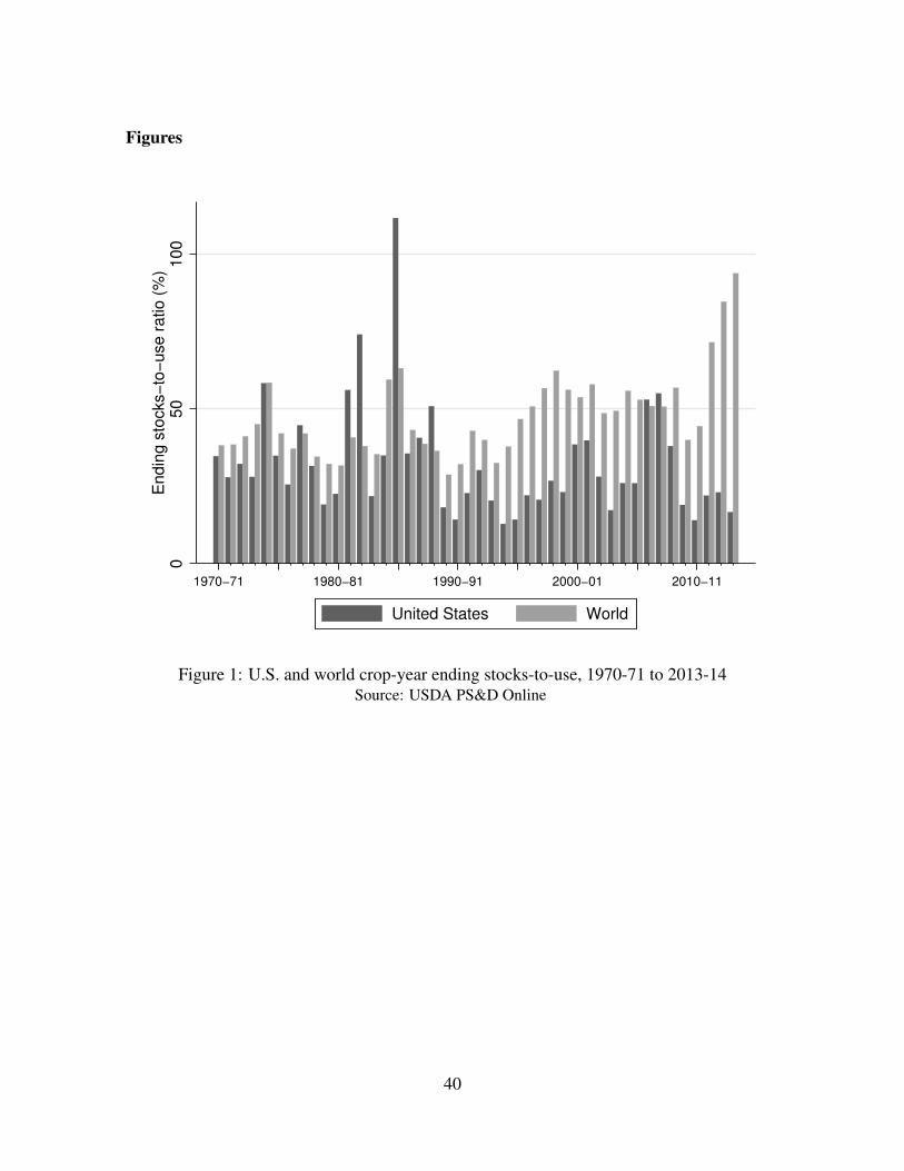
Figures

05

01

00

En

din

g s

tocks−

to−

use

ra

tio

(%

)

1970−71 1980−81 1990−91 2000−01 2010−11

United States World

Figure 1: U.S. and world crop-year ending stocks-to-use, 1970-71 to 2013-14Source: USDA PS&D Online

40

Panel A: Price-Quantity Equilibrium Panel B: Price-Inventory Equilibrium

Panel C: Spread-Inventory Equilibrium

Inventory

Inventory

Quantity

Pric

e

Pric

e

Pt

It

Et(Pt+1)− Pt

Dt Dt + It

g(It)

j(It)h(St + It−1)

f(Dt) + g(It)F (Dt)

Figure 2: Price, spread, and inventory determination in a stylized single-period representationof the competitive storage model

41

−1

−.5

0.5

1E

co

no

mic

Activity

Jan 1970 Jan 1975 Jan 1980 Jan 1985 Jan 1990 Jan 1995 Jan 2000 Jan 2005 Jan 2010 Jan 2015

−1

−.5

0.5

1G

SC

I

Jan 1970 Jan 1975 Jan 1980 Jan 1985 Jan 1990 Jan 1995 Jan 2000 Jan 2005 Jan 2010 Jan 2015

−1

−.5

0.5

1C

rud

e O

il P

rice

Jan 1970 Jan 1975 Jan 1980 Jan 1985 Jan 1990 Jan 1995 Jan 2000 Jan 2005 Jan 2010 Jan 2015

−.6

−.4

−.2

0.2

Co

tto

n S

pre

ad

Jan 1970 Jan 1975 Jan 1980 Jan 1985 Jan 1990 Jan 1995 Jan 2000 Jan 2005 Jan 2010 Jan 2015

−1

−.5

0.5

1C

ott

on

Price

Jan 1970 Jan 1975 Jan 1980 Jan 1985 Jan 1990 Jan 1995 Jan 2000 Jan 2005 Jan 2010 Jan 2015Date

Figure 3: Data plot for variables in yt, controlling for linear trend and seasonality, July 1970to June 2014

42

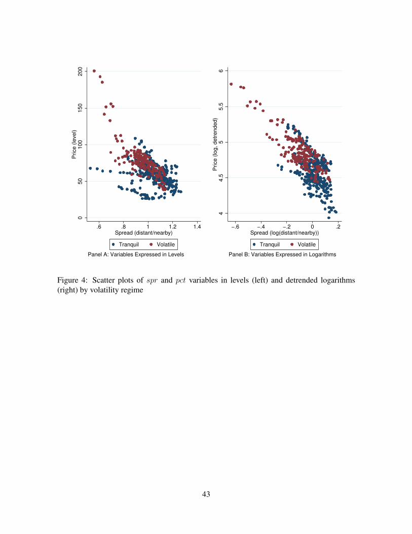
050

100

150

200

Price (

level)

.6 .8 1 1.2 1.4Spread (distant/nearby)

Tranquil Volatile

Panel A: Variables Expressed in Levels

44.5

55.5

6P

rice (

log, detr

ended)

−.6 −.4 −.2 0 .2Spread (log(distant/nearby))

Tranquil Volatile

Panel B: Variables Expressed in Logarithms

Figure 4: Scatter plots of spr and pct variables in levels (left) and detrended logarithms(right) by volatility regime

43

Figure 5: Impulse response functions generated from SVAR with GSCI as external market

44

Figure 6: Historical decomposition of structural shocks with the GSCI as external market

45

Figure 7: Counterfactual analysis of cotton prices, 2006-2014, for SVAR with GSCI as ex-ternal market

46

Figure 8: Historical decomposition of structural shocks with crude oil as external market

47

Figure 9: Counterfactual analysis of cotton prices, 2006-2014, for SVAR with crude oil asexternal market

48

Figure 10: Historical decomposition of cotton prices, 1970-2014, generated using StructuralFactor Augmented VAR

49

Figure 11: Counterfactual analysis of cotton prices, 2006-2014, generated using StructuralFactor Augmented VAR

50

Tables

Table 1: Reduced-form VAR Regression Results

Equationrea ext spr pct

Intercept 0.022 0.116∗∗ 0.062 0.099(0.101) (0.046) (0.049) (0.072)

reat−1 1.102∗∗ 0.031 0.039 -0.017(0.069) (0.027) (0.027) (0.044)

extt−1 0.183∗ 1.220∗∗ -0.042 0.122∗

(0.092) (0.052) (0.043) (0.071)sprt−1 0.2304∗ 0.214∗∗ 0.599∗∗ 0.569∗∗

(0.122) (0.064) (0.147) (0.190)pctt−1 0.209∗ 0.195∗∗ -0.228∗∗ 1.427∗∗

(0.093) (0.055) (0.068) (0.099)reat−2 -0.161∗∗ -0.019 -0.026 0.006

(0.068) (0.028) (0.027) (0.044)extt−2 -0.179∗ -0.228∗∗ 0.041 -0.110

(0.091) (0.053) (0.042) (0.070)sprt−2 -0.250∗ -0.264∗∗ 0.279∗ -0.502∗∗

(0.121) (0.067) (0.143) (0.188)pctt−2 -0.223∗∗ -0.215∗∗ 0.212∗∗ -0.456∗∗

(0.091) (0.055) (0.066) (0.097)

Note: Heteroskedasticity-robust standard errors are in parentheses. ∗ and∗∗ denote significance at the 5% and 1% levels. Coefficient estimates forseasonal indicators and linear time trend are not reported.

51

Table 2: Structural vector autoregression model parameter estimates

ParameterA0 1 0 0 0

-0.084 1 0 0-0.032 -0.026 1 0.711-0.126 -0.107 -3.209 1

RegimeParameter Tranquil VolatileΩr 0.491 0.043 -0.009 0.034 0.491 0.043 -0.009 0.034

0.043 0.183 0.003 0.040 0.043 0.183 0.003 0.040-0.009 0.003 0.156 -0.186 -0.009 0.003 0.221 -0.2840.034 0.040 -0.186 0.369 0.034 0.040 -0.284 0.479

σREA 0.491 0.491σCM 0.179 0.179σPD 0.073 0.054σNS 3.025 4.369

Note: For ease of presentation, we report the estimated variance and co-variance parameters multiplied by 100 and we include a box around thereduced-form parameters that vary by regime.

52

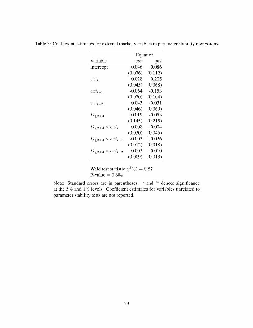
Table 3: Coefficient estimates for external market variables in parameter stability regressions

EquationVariable spr pctIntercept 0.046 0.086

(0.076) (0.112)extt 0.028 0.205

(0.045) (0.068)extt−1 -0.064 -0.153

(0.070) (0.104)extt−2 0.043 -0.051

(0.046) (0.069)D≥2004 0.019 -0.053

(0.145) (0.215)D≥2004 × extt -0.008 -0.004

(0.030) (0.045)D≥2004 × extt−1 -0.003 0.026

(0.012) (0.018)D≥2004 × extt−2 0.005 -0.010

(0.009) (0.013)

Wald test statistic χ2(8) = 8.87P-value = 0.354

Note: Standard errors are in parentheses. ∗ and ∗∗ denote significanceat the 5% and 1% levels. Coefficient estimates for variables unrelated toparameter stability tests are not reported.

53