1

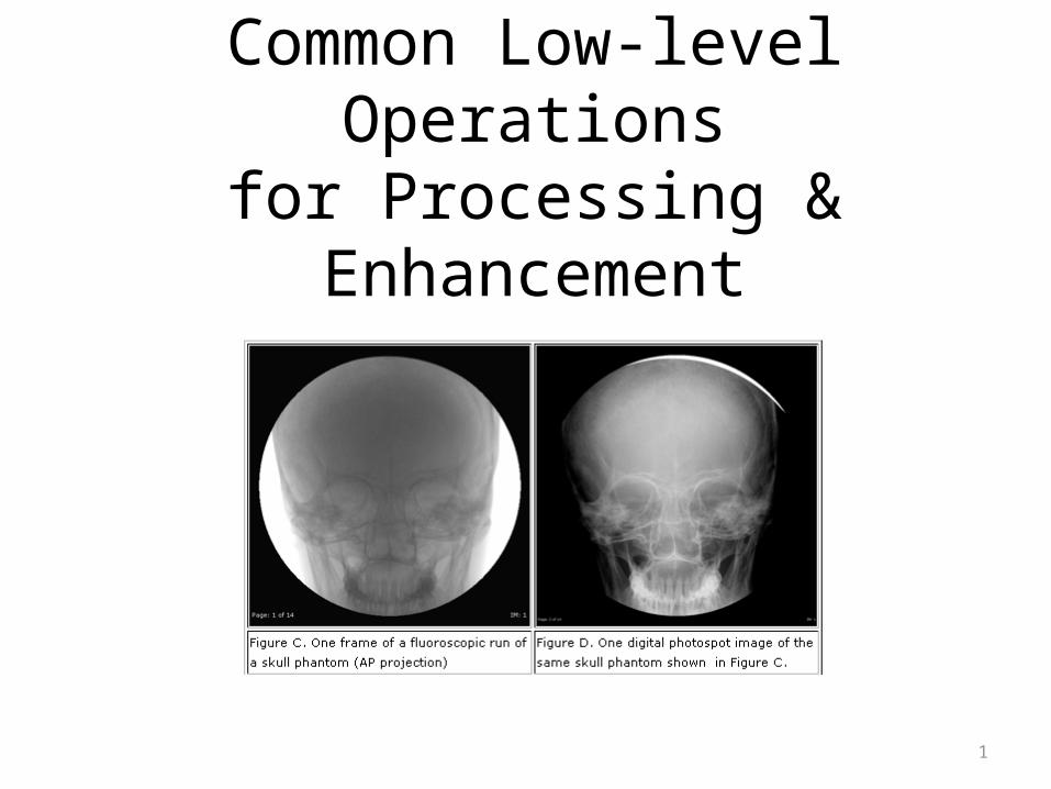
Common Low-level Operationsfor Processing & Enhancement

2

Histogram Equalization

• A histogram of image I is a data structure h in which h(i) is the number of pixels in I that have value i. Usually 0 <= i <= 255.

• A normalized histogram is a histogram in which each value is divided by the total number of pixels in the image. These normalized values are often thought of as probabilities Pr(i) of the different pixel values.

3

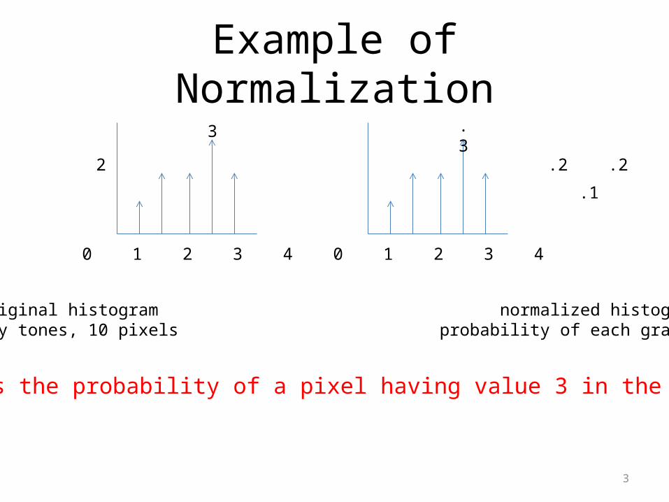
Example of Normalization

0 1 2 3 4 0 1 2 3 4

1 .1

2 2 2 .2 .2 .2

3

.3

original histogram normalized histogram5 gray tones, 10 pixels probability of each gray tone

What’s the probability of a pixel having value 3 in the image?

4

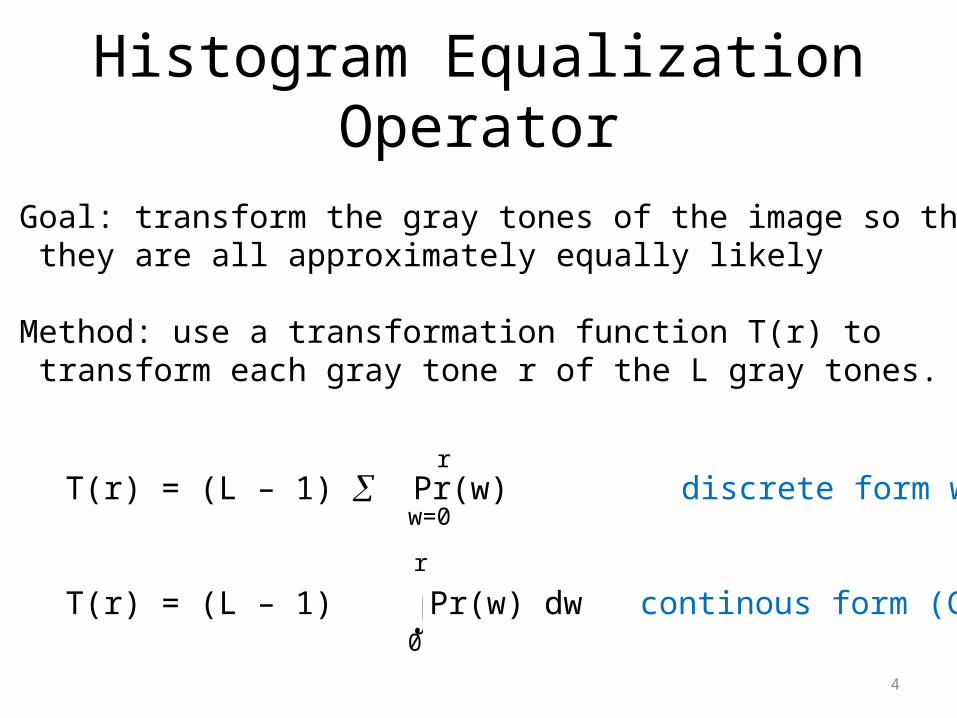
Histogram Equalization Operator

• Goal: transform the gray tones of the image so that they are all approximately equally likely

• Method: use a transformation function T(r) to transform each gray tone r of the L gray tones.

T(r) = (L – 1) Pr(w) discrete form we use

T(r) = (L – 1) Pr(w) dw continous form (CDF)

r

w=0

r

0

5

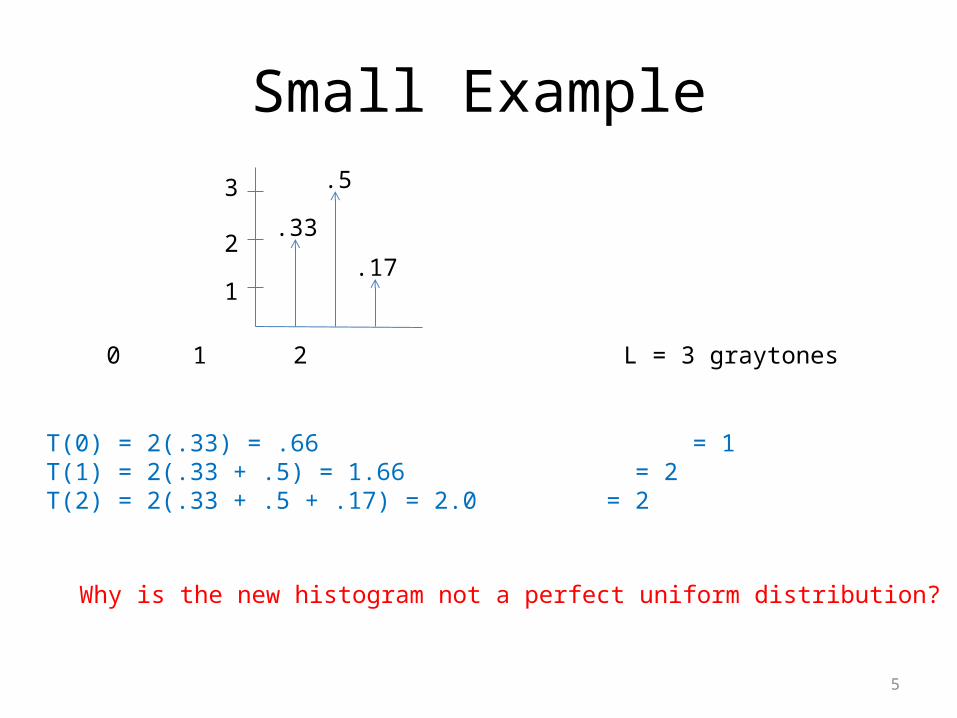
Small Example

0 1 2 L = 3 graytones

1

2

3

.33

.5

.17

T(0) = 2(.33) = .66 = 1T(1) = 2(.33 + .5) = 1.66 = 2T(2) = 2(.33 + .5 + .17) = 2.0 = 2

Why is the new histogram not a perfect uniform distribution?

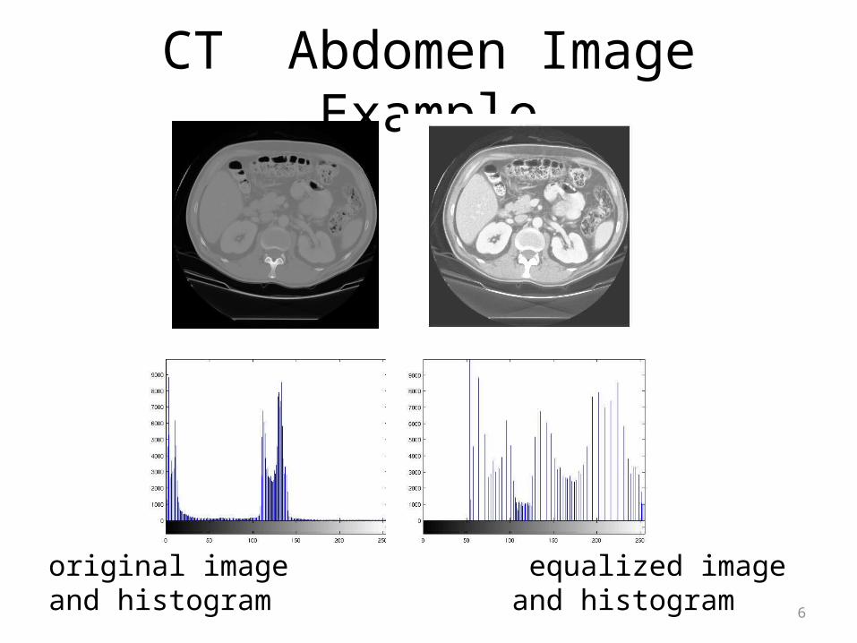
6

CT Abdomen Image Example

original image equalized imageand histogram and histogram

7

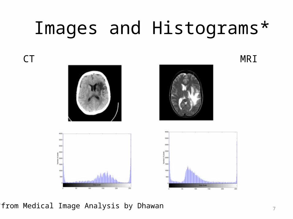
Images and Histograms*

CT MRI

*from Medical Image Analysis by Dhawan

8

Histogram Equalization

9

Image Averaging and Subtraction

• If images are noisy, multiple images may be taken and averaged to produce a new image that is smoothed.

• Image subtraction to show differences over time or with and without a dye or tracer.

10

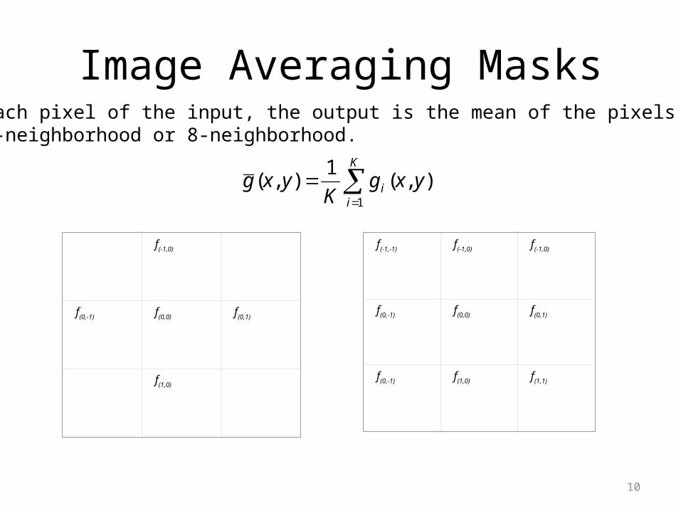
Image Averaging Masks

K

ii yxg

Kyxg

1

),(1

),(

 

  f(-1,0)  

f(0,-1) f(0,0) f(0,1)

  f(1,0)  

f(-1,-1) f(-1,0) f(-1,0)

f(0,-1) f(0,0) f(0,1)

f(0,-1) f(1,0) f(1,1)

 

For each pixel of the input, the output is the mean of the pixels inits 4-neighborhood or 8-neighborhood.

11

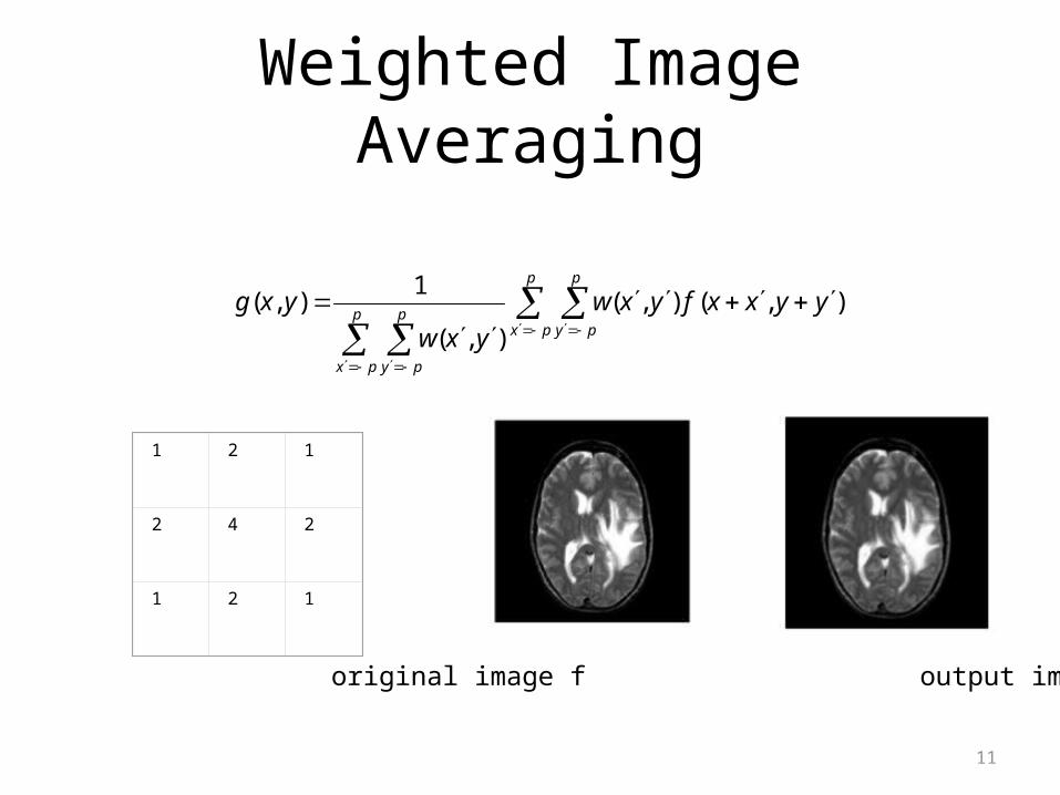
Weighted Image Averaging

p

px

p

pyp

px

p

py

yyxxfyxw

yxw

yxg ),(),(

),(

1),(

 

1 2 1

2 4 2

1 2 1

original image f output image g

12

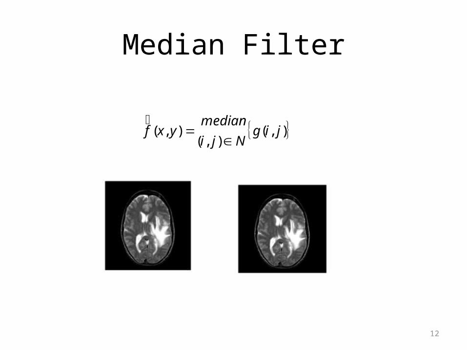
Median Filter

),(),(

),( jigNji

medianyxf

13

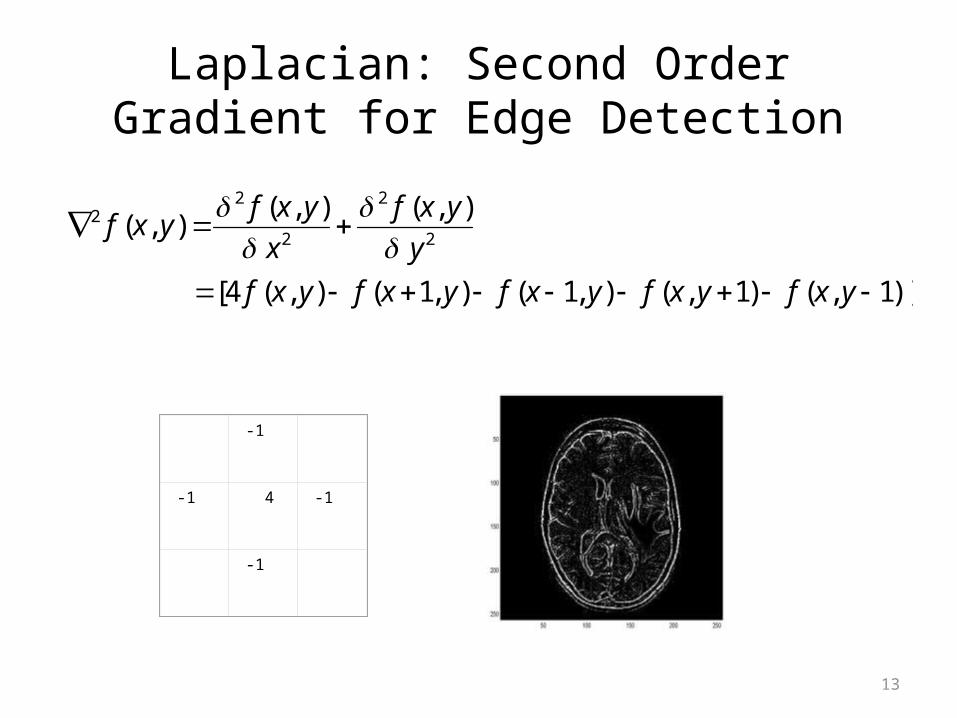
Laplacian: Second Order Gradient for Edge Detection

)]1,()1,(),1(),1(),(4[

),(

),(),(

2

2

2

22

yxfyxfyxfyxfyxf

y

yxf

x

yxfyxf

 

-1

-1 4 -1

-1

14

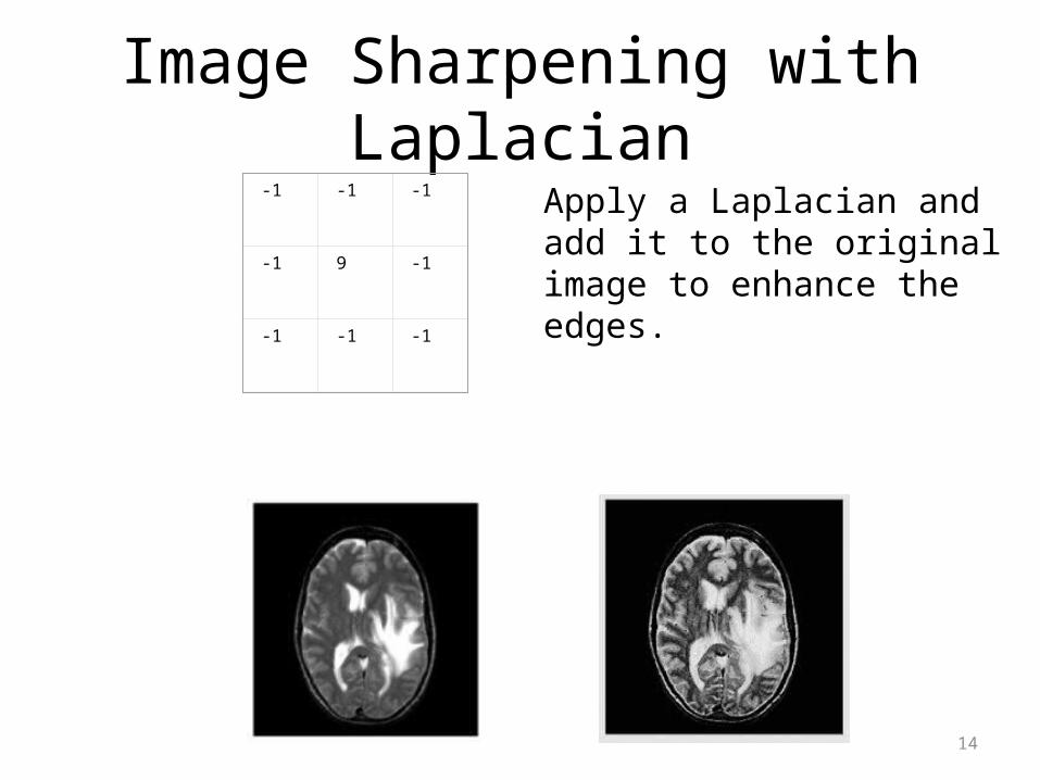
Image Sharpening with Laplacian

 

-1 -1 -1

-1 9 -1

-1 -1 -1

Apply a Laplacian andadd it to the originalimage to enhance theedges.

15

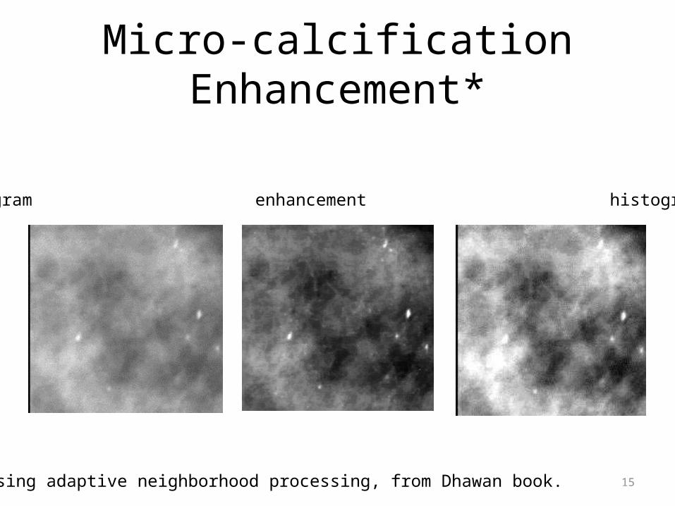
Micro-calcification Enhancement*

* Using adaptive neighborhood processing, from Dhawan book.

original mammogram enhancement histogram equalization

16

Frequency-Domain Methods

• Convert the image from the spatial domain to the frequency domain via a Fourier Transform

• Apply filters in the frequency domain

• Convert back to the spatial domain

• Used to emphasize or de-emphasize specified frequency components

17

Fourier Transform Basics

• complex numbers• complex exponentials• Euler’s formula• nth roots of unity• orthogonal basis• 1D discrete Fourier transform• 2D discrete Fourier transform• examples

18

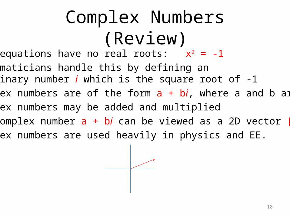
Complex Numbers (Review)• Some equations have no real roots: x2 = -1• Mathematicians handle this by defining an imaginary number i which is the square root of -1• Complex numbers are of the form a + bi, where a and b are real• Complex numbers may be added and multiplied• The complex number a + bi can be viewed as a 2D vector [a,b]• Complex numbers are used heavily in physics and EE.

19

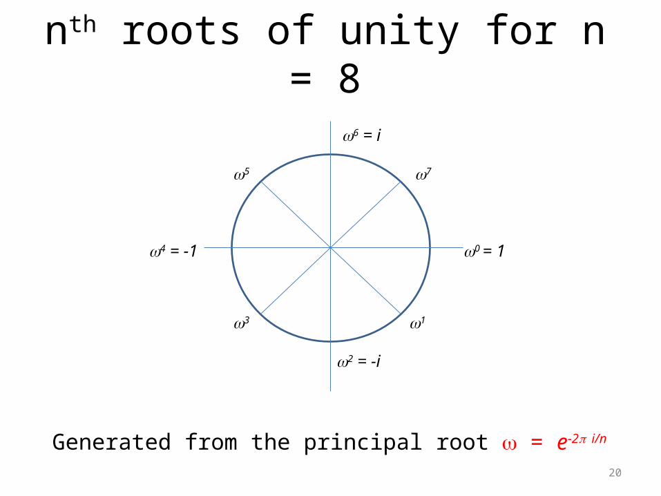
Complex Exponentials• Euler’s Formula: ei = cos + i sin • Thus raising e to a power corresponds to taking the sine and cosine of an angle• ei is a periodic function; when = 0 or multiples of 2, it has value 1.• = e-2 i/n is an n-th root of one for any integer nExample with n = 8 • 0 = (e-2 i/8)0 = 1

• 1 = (e-2 i/8)1 = e(-/4)i = cos(-/4) + isin(-/4) = sqrt(2)/2 – sqrt(2)/2i• 2 = (e-2 i/8)2 = e(-/2)i = cos(-/2) + isin(-/2) = -i• etc.

20

nth roots of unity for n = 8

0 = 1

1

2 = -i

3

4 = -1

5

6 = i

7

Generated from the principal root = e-2 i/n

21

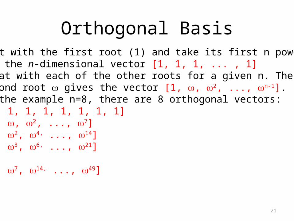
Orthogonal Basis• Start with the first root (1) and take its first n powers to get the n-dimensional vector [1, 1, 1, ... , 1] • Repeat with each of the other roots for a given n. The second root gives the vector [1, , 2, ..., n-1].• For the example n=8, there are 8 orthogonal vectors:• [1, 1, 1, 1, 1, 1, 1, 1]• [1, , 2, ..., 7]• [1, 2, 4, ..., 14]• [1, 3, 6, ..., 21]• ...• [1, 7, 14, ..., 49]

22

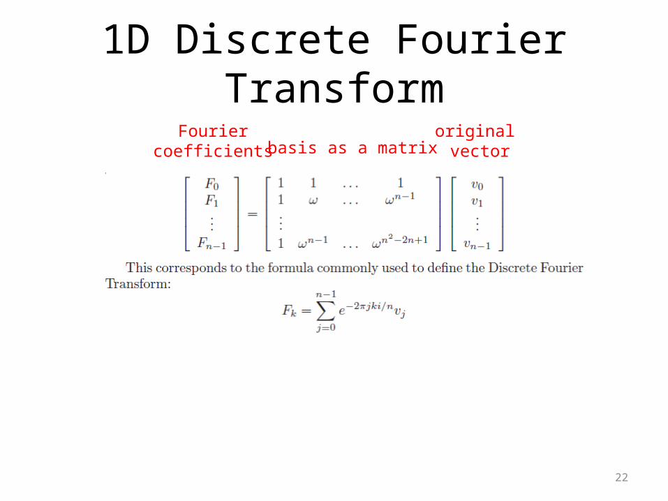
1D Discrete Fourier Transformoriginal vectorbasis as a matrix

Fouriercoefficients

23

2D Discrete Fourier Transform• Detect the frequency components of the image in both the horizontal and vertical directions• First apply the 1D discrete Fourier transform to each row of the image, producing an intermediate image or row transforms• Then apply the 1D discrete Fourier transform to each column of the intermediate image• The result is the 2D discrete Fourier transform of the image, which is an image in the frequency domain.

24

Filtering with the Fourier Transform

1. Compute the 2D discrete Fourier transform of the image2. Apply an image operator to the transformed image3. Computer the inverse 2D discrete Fourier transform of the result of the image operator

Two most common filters:1. low-pass filtering zeroes out the frequency components above a threshold 2. high-pass filtering zeroes out the frequency components below a threshold

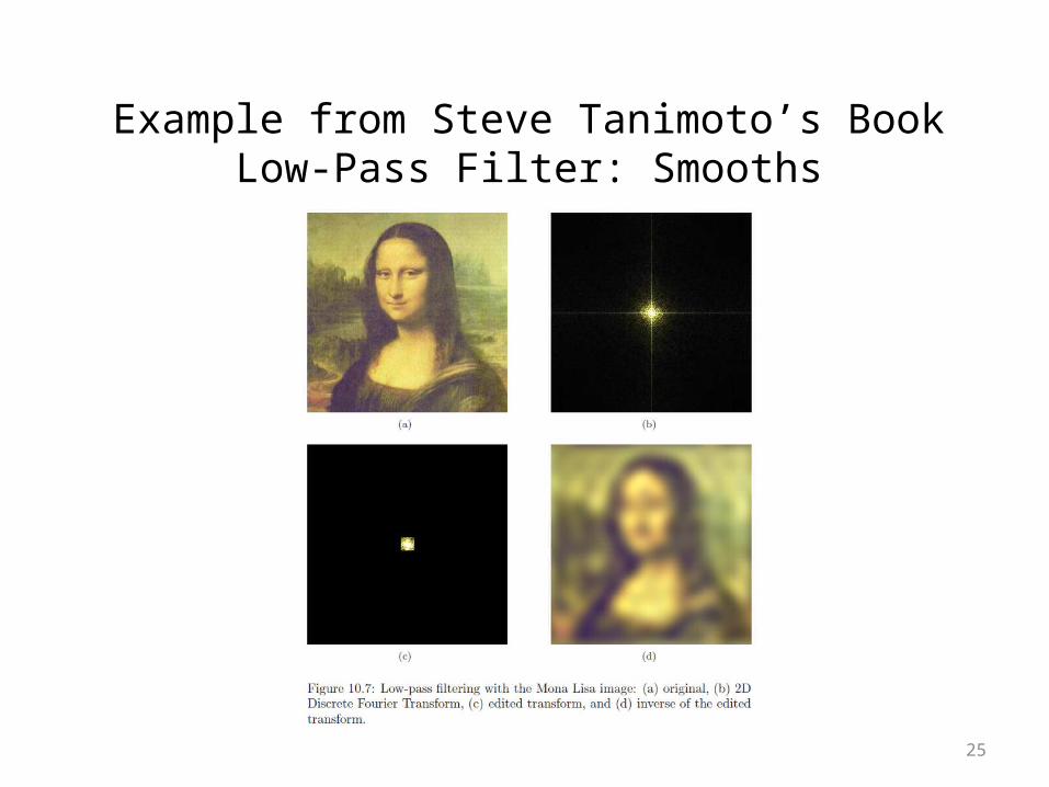
25

Example from Steve Tanimoto’s BookLow-Pass Filter: Smooths

26

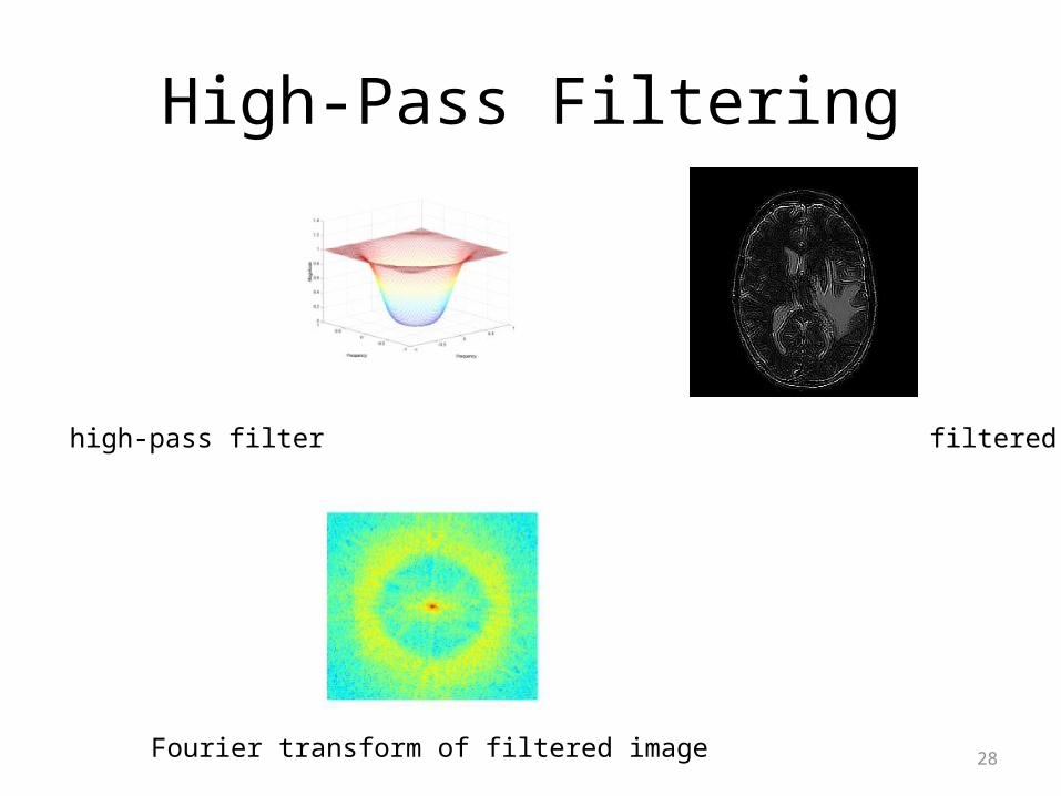
High-Pass Filter: Finds Edges

27

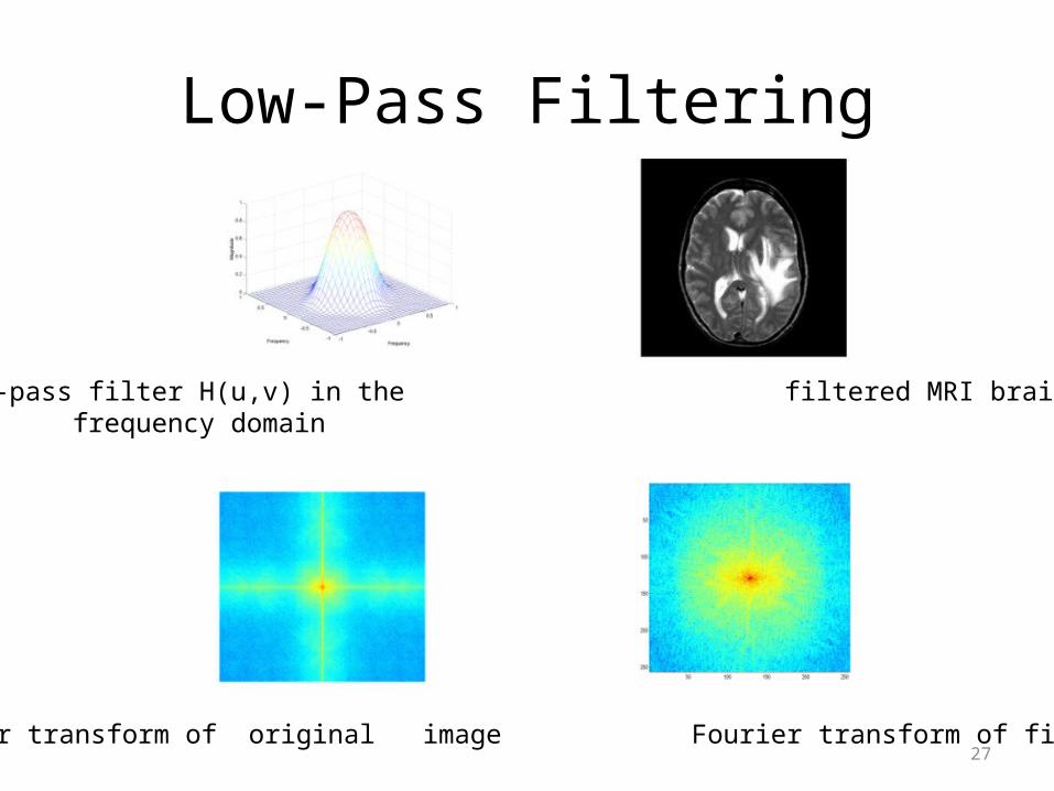
Low-Pass Filtering

low-pass filter H(u,v) in the filtered MRI brain image frequency domain

Fourier transform of original image Fourier transform of filtered image

28

High-Pass Filtering

high-pass filter filtered image

Fourier transform of filtered image

29

Wavelet Transform Fourier Transform only provides frequency

information. Wavelet Transform is a method for complete

time-frequency localization for signal analysis and characterization.

Wavelet Transform : works like a microscope focusing on finer time resolution as the scale becomes small to see how the impulse gets better localized at higher frequency permitting a local characterization

30

Basics of Wavelets*

• Wavelets are a mathematical tool for hierarchically decomposing functions.• They allow a function to be described in terms of a coarse overall shape, plus details than range from narrow to broad.• Wavelets represent the signal or image as a linear combination of basis functions.• The simplest basis is the Haar wavelet basis.

* Material from Stollnitz et al., Wavelets for Computer Graphics: A Primer Part 1.

31

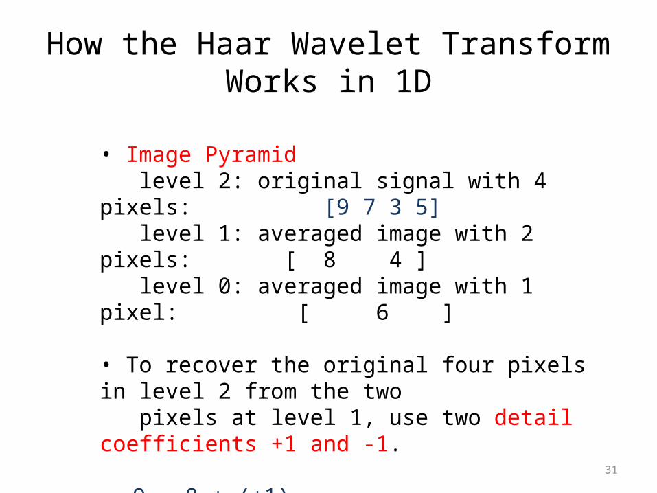
How the Haar Wavelet Transform Works in 1D

• Image Pyramid level 2: original signal with 4 pixels: [9 7 3 5] level 1: averaged image with 2 pixels: [ 8 4 ] level 0: averaged image with 1 pixel: [ 6 ]

• To recover the original four pixels in level 2 from the two pixels at level 1, use two detail coefficients +1 and -1.

9 = 8 + (+1)7 = 8 – (+1)3 = 4 + (-1)5 = 4 – (-1)

32

level 2: [9 7 3 5]level 1: [ 8 4 ]level 0: [ 6 ]

• To recover the two pixels in level 1 from the one pixels at level 0, use one detail coefficient of 2.

8 = 6 + 2 4 = 6 - 2

• The wavelet transform of the original 4-pixel image is [ 6 2 1 -1 ]

• It has the same number of coefficients as the original image, but it lets us reconstruct the image at any resolution.

33

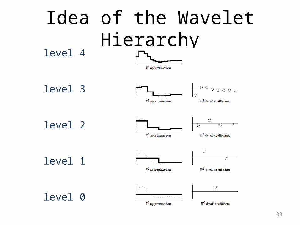
Idea of the Wavelet Hierarchylevel 4

level 3

level 2

level 1

level 0

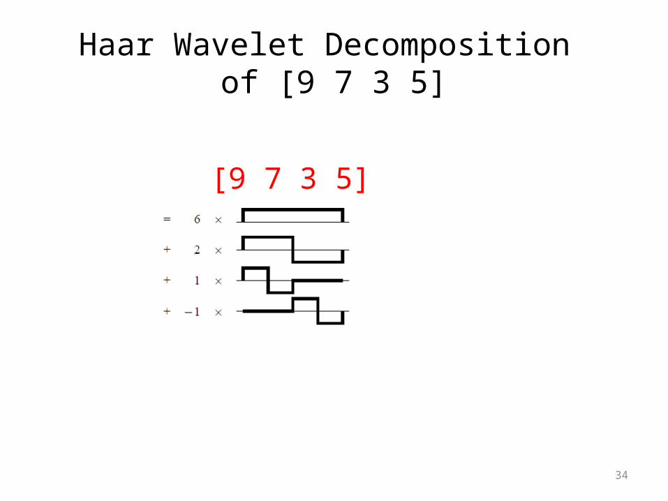
Haar Wavelet Decomposition of [9 7 3 5]

34

[9 7 3 5]

35

Two-Dimensional Haar Wavelet Transform: Standard Decomposition

• First apply the 1D wavelet transform to each row of pixel values• This gives an average value along with detail coefficients for each row• Next treat these transformed rows as an image and apply the 1D transform to each column• The resulting values are all detail coefficients except for the single overall average coefficient

36

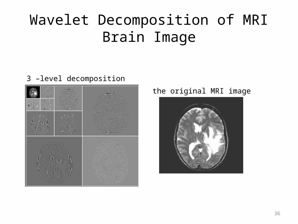
Wavelet Decomposition of MRI Brain Image

the original MRI image

3 –level decomposition

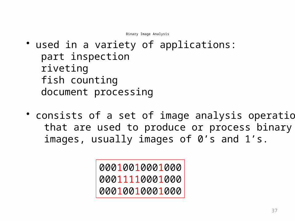
Binary Image Analysis

• used in a variety of applications: part inspectionrivetingfish countingdocument processing

• consists of a set of image analysis operations that are used to produce or process binary images, usually images of 0’s and 1’s.

000100100010000001111000100000010010001000

37

Example: red blood cell image

• Many blood cells are separate objects

• Many touch – bad!

• Salt and pepper noise from thresholding

• What operations are needed to clean it up?

38

39

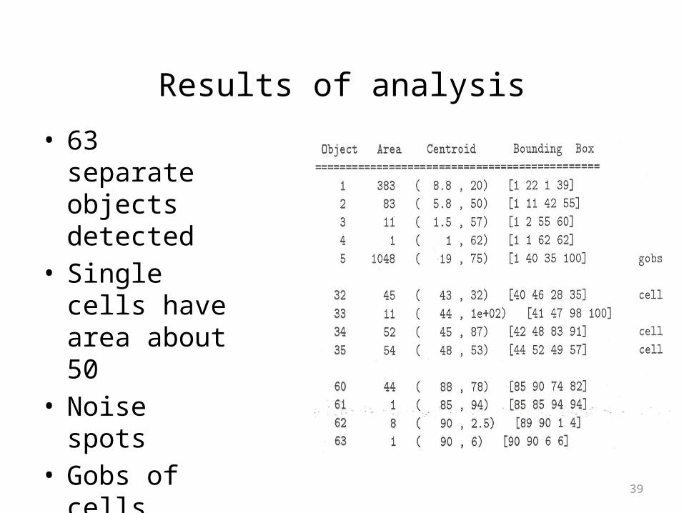
Results of analysis

• 63 separate objects detected

• Single cells have area about 50

• Noise spots• Gobs of cells

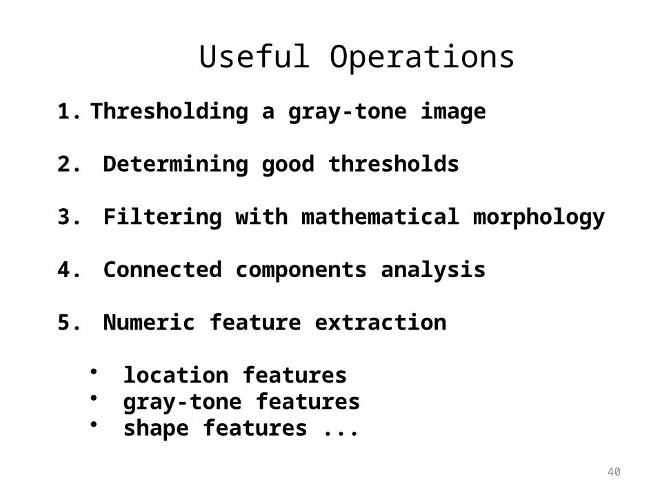
Useful Operations

1. Thresholding a gray-tone image

2. Determining good thresholds

3. Filtering with mathematical morphology

4. Connected components analysis

5. Numeric feature extraction

• location features• gray-tone features• shape features ...

40

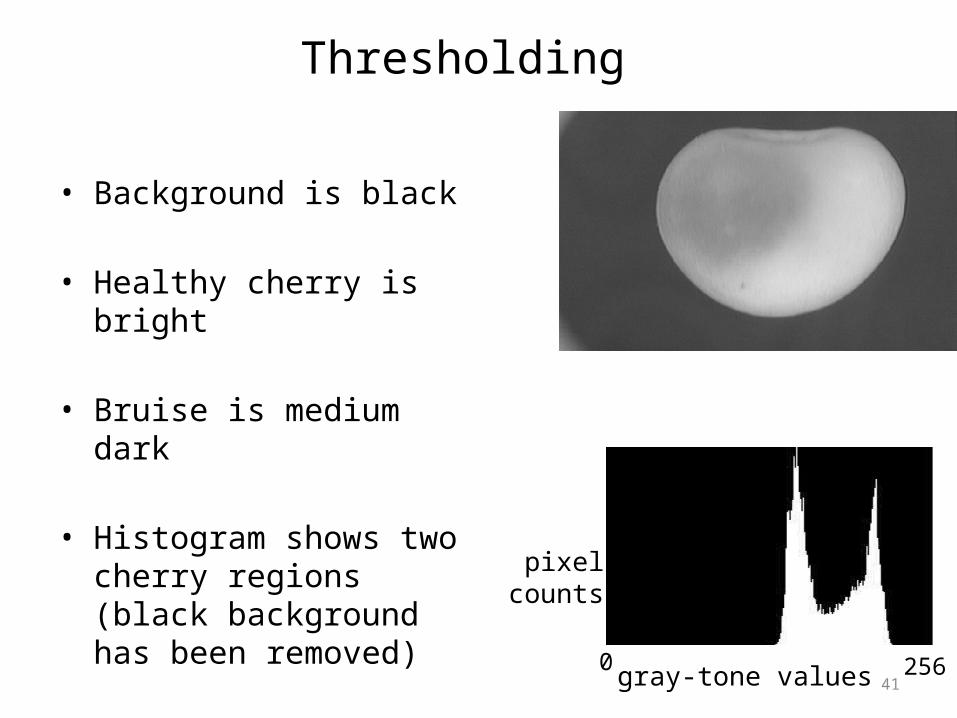
Thresholding

• Background is black

• Healthy cherry is bright

• Bruise is medium dark

• Histogram shows two cherry regions (black background has been removed)

gray-tone values

pixelcounts

0 25641

42

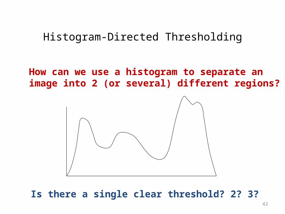
Histogram-Directed Thresholding

How can we use a histogram to separate animage into 2 (or several) different regions?

Is there a single clear threshold? 2? 3?

43

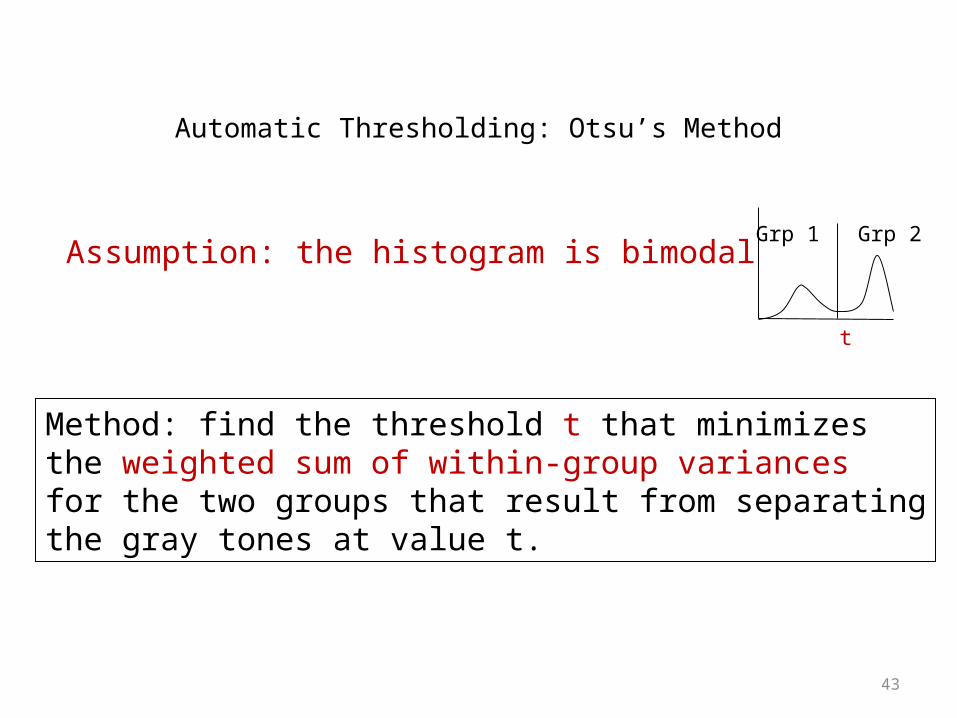
Automatic Thresholding: Otsu’s Method

Assumption: the histogram is bimodal

t

Method: find the threshold t that minimizesthe weighted sum of within-group variancesfor the two groups that result from separatingthe gray tones at value t.

Grp 1 Grp 2

44

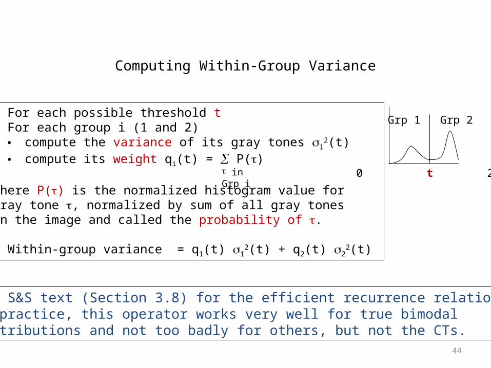
Computing Within-Group Variance

t

See S&S text (Section 3.8) for the efficient recurrence relations;in practice, this operator works very well for true bimodal distributions and not too badly for others, but not the CTs.

Grp 1 Grp 2• For each possible threshold t• For each group i (1 and 2)• compute the variance of its gray tones i

2(t) • compute its weight qi(t) = P()

where P() is the normalized histogram value forgray tone , normalized by sum of all gray tonesin the image and called the probability of .

• Within-group variance = q1(t) 12(t) + q2(t) 2

2(t)

t in Grp i 0 255

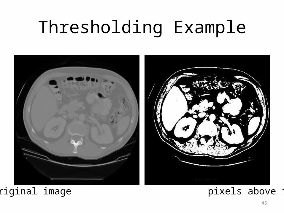
Thresholding Example

original image pixels above threshold45

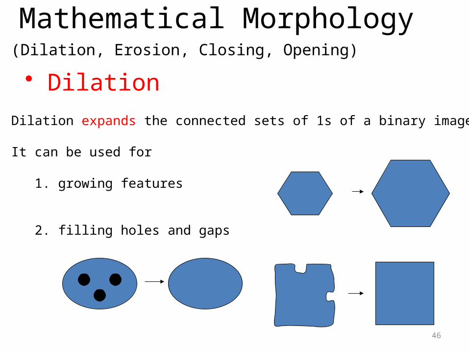
Dilation expands the connected sets of 1s of a binary image.

It can be used for

1. growing features

2. filling holes and gaps

Mathematical Morphology(Dilation, Erosion, Closing, Opening)

• Dilation

46

• Erosion

Erosion shrinks the connected sets of 1s of a binary image.

It can be used for

1. shrinking features

2. Removing bridges, branches and small protrusions

47

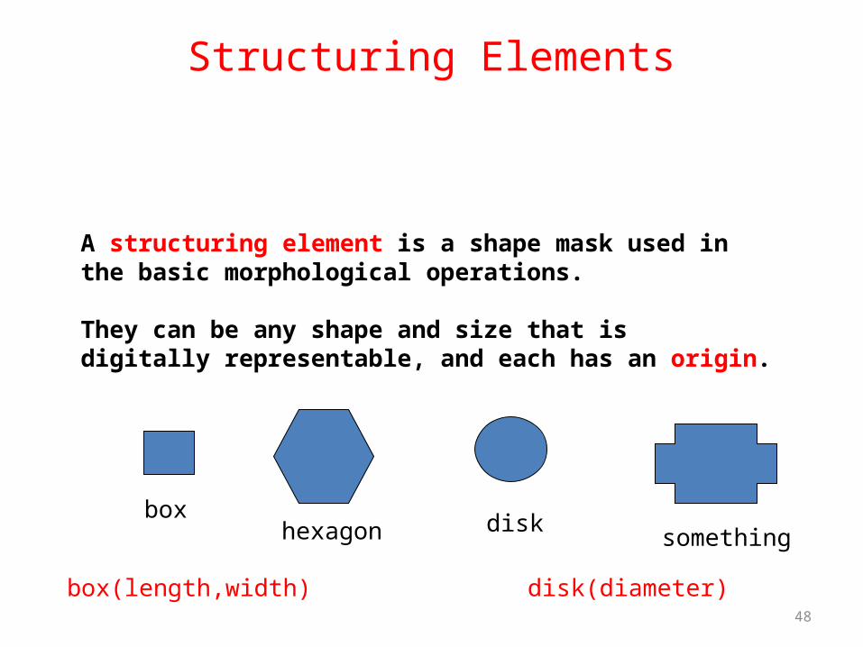
Structuring Elements

A structuring element is a shape mask used inthe basic morphological operations.

They can be any shape and size that isdigitally representable, and each has an origin.

boxhexagon disk

something

box(length,width) disk(diameter)48

Dilation with Structuring Elements

The arguments to dilation and erosion are

1. a binary image B2. a structuring element S

dilate(B,S) takes binary image B, places the originof structuring element S over each 1-pixel, and ORsthe structuring element S into the output image atthe corresponding position.

0 0 0 00 1 1 00 0 0 0

11 1

0 1 1 00 1 1 10 0 0 0

originBS

dilate

B S49

Erosion with Structuring Elements

erode(B,S) takes a binary image B, places the origin of structuring element S over every pixel position, andORs a binary 1 into that position of the output image only ifevery position of S (with a 1) covers a 1 in B.

0 0 1 1 00 0 1 1 00 0 1 1 01 1 1 1 1

111

0 0 0 0 00 0 1 1 00 0 1 1 00 0 0 0 0

B S

origin

erode

B S

50

Opening and Closing

• Closing is the compound operation of dilation followed by erosion (with the same structuring element)

• Opening is the compound operation of erosion followed by dilation (with the same structuring element)

51

52

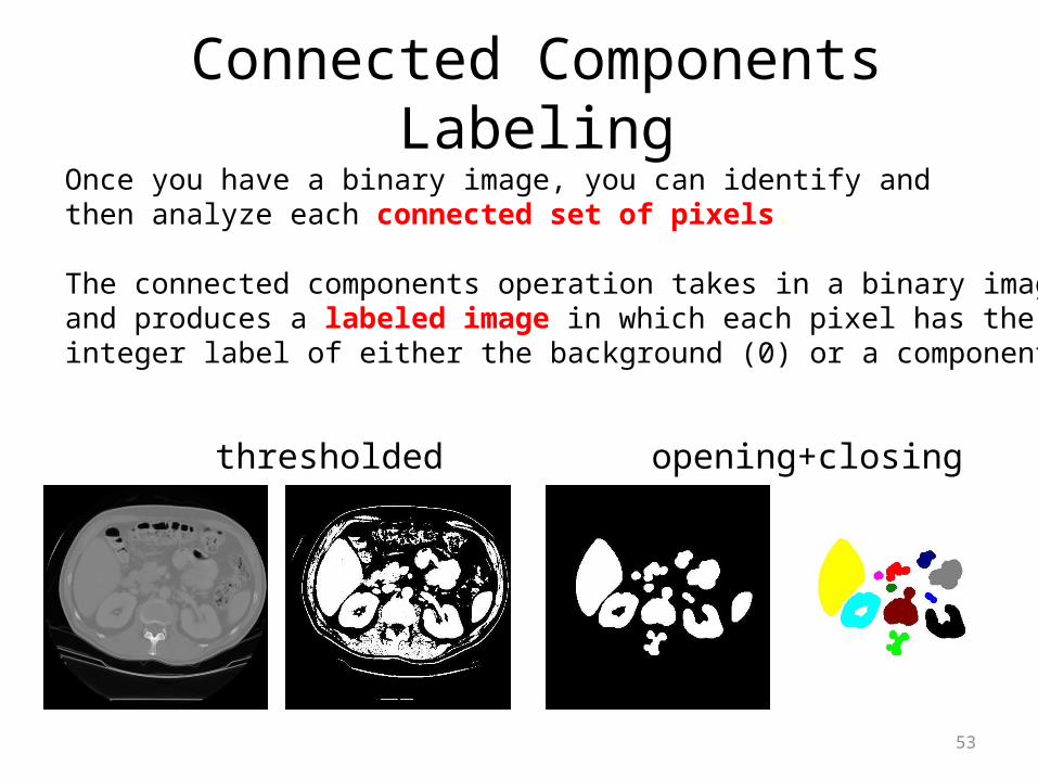
Connected Components LabelingOnce you have a binary image, you can identify and then analyze each connected set of pixels.

The connected components operation takes in a binary image and produces a labeled image in which each pixel has the integer label of either the background (0) or a component.

original thresholded opening+closing components

53

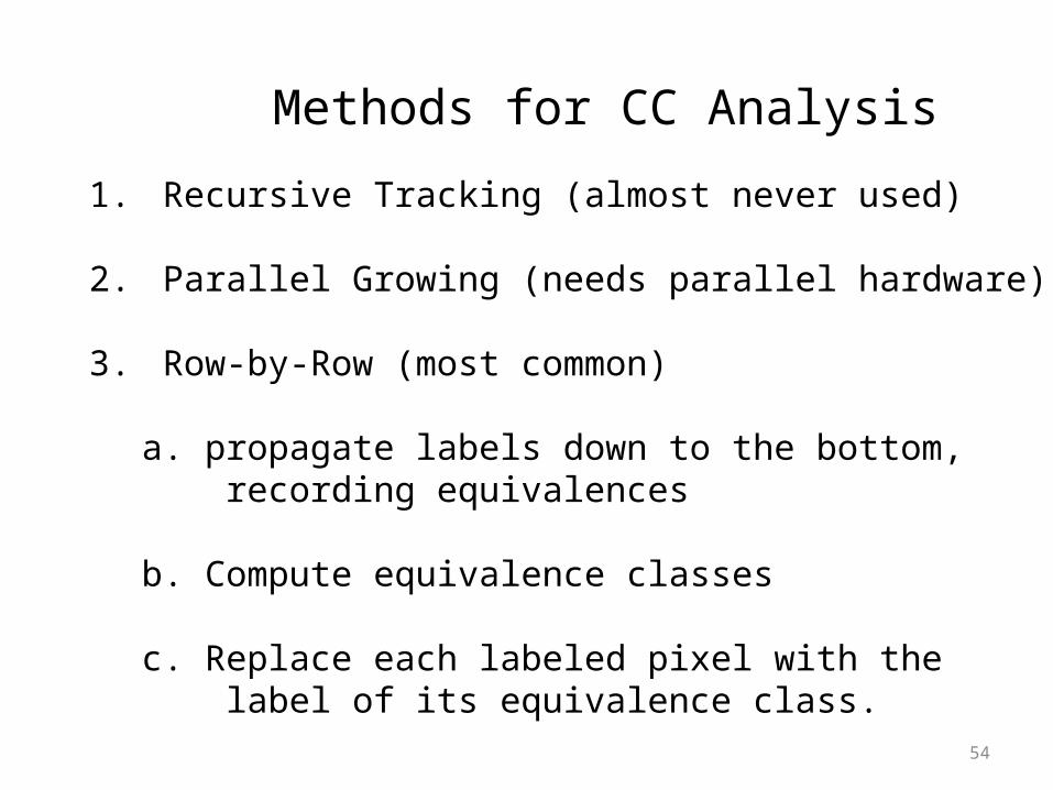
Methods for CC Analysis

1. Recursive Tracking (almost never used)

2. Parallel Growing (needs parallel hardware)

3. Row-by-Row (most common)

a. propagate labels down to the bottom, recording equivalences

b. Compute equivalence classes

c. Replace each labeled pixel with the label of its equivalence class.

54

55

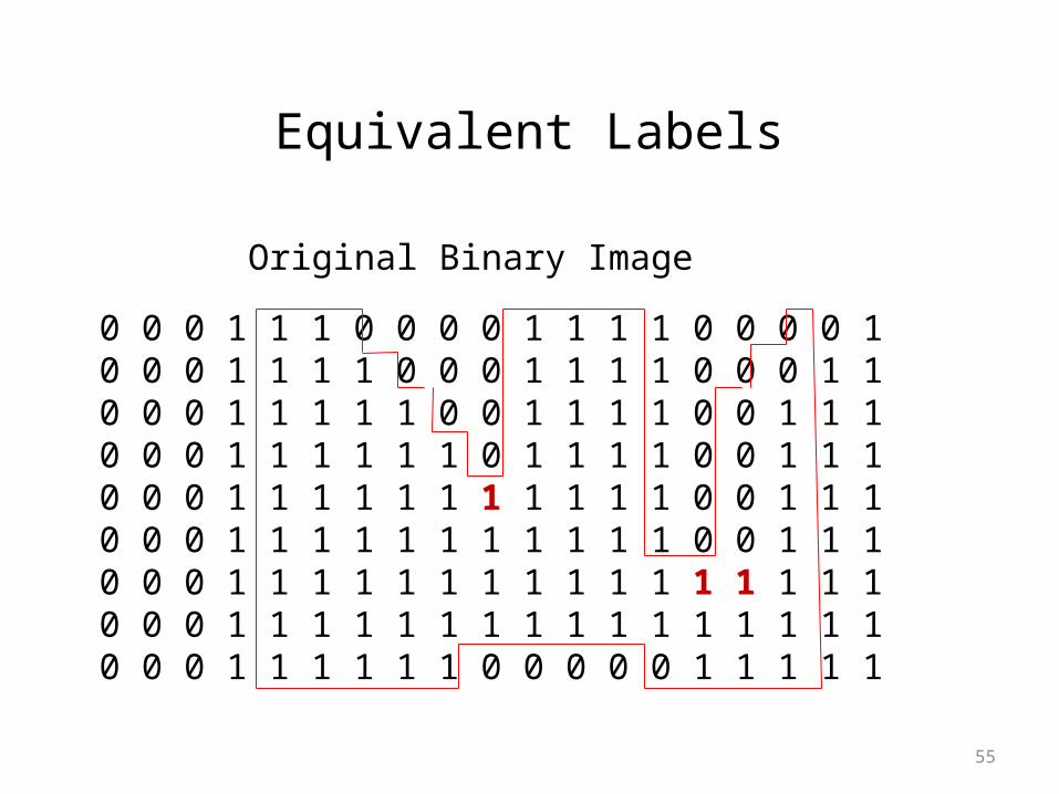
Equivalent Labels

0 0 0 1 1 1 0 0 0 0 1 1 1 1 0 0 0 0 10 0 0 1 1 1 1 0 0 0 1 1 1 1 0 0 0 1 10 0 0 1 1 1 1 1 0 0 1 1 1 1 0 0 1 1 10 0 0 1 1 1 1 1 1 0 1 1 1 1 0 0 1 1 10 0 0 1 1 1 1 1 1 1 1 1 1 1 0 0 1 1 10 0 0 1 1 1 1 1 1 1 1 1 1 1 0 0 1 1 10 0 0 1 1 1 1 1 1 1 1 1 1 1 1 1 1 1 10 0 0 1 1 1 1 1 1 1 1 1 1 1 1 1 1 1 10 0 0 1 1 1 1 1 1 0 0 0 0 0 1 1 1 1 1

Original Binary Image

56

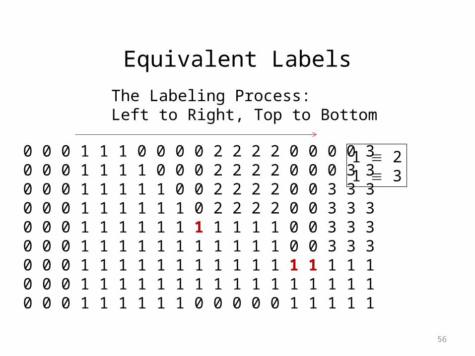
Equivalent Labels

0 0 0 1 1 1 0 0 0 0 2 2 2 2 0 0 0 0 30 0 0 1 1 1 1 0 0 0 2 2 2 2 0 0 0 3 30 0 0 1 1 1 1 1 0 0 2 2 2 2 0 0 3 3 30 0 0 1 1 1 1 1 1 0 2 2 2 2 0 0 3 3 30 0 0 1 1 1 1 1 1 1 1 1 1 1 0 0 3 3 30 0 0 1 1 1 1 1 1 1 1 1 1 1 0 0 3 3 30 0 0 1 1 1 1 1 1 1 1 1 1 1 1 1 1 1 10 0 0 1 1 1 1 1 1 1 1 1 1 1 1 1 1 1 10 0 0 1 1 1 1 1 1 0 0 0 0 0 1 1 1 1 1

The Labeling Process: Left to Right, Top to Bottom

1 21 3

57

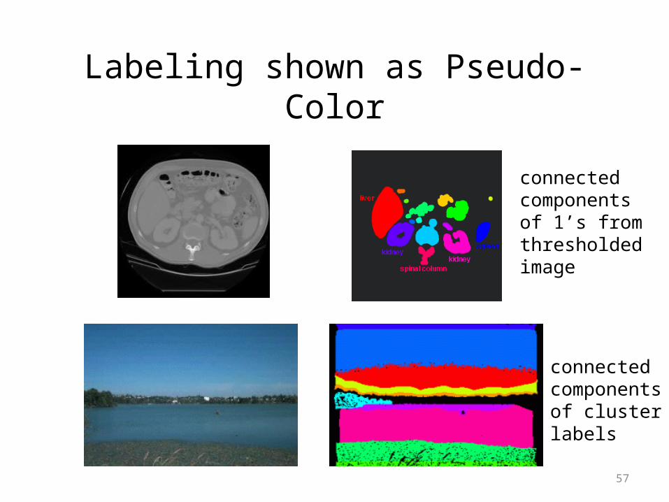
Labeling shown as Pseudo-Color

connectedcomponentsof 1’s fromthresholdedimage

connectedcomponentsof clusterlabels