Communication-Driven Localization andMapping for Millimeter Wave Networks

Joan Palacios]‡, Guillermo Bielsa]‡, Paolo Casari], Joerg Widmer]]IMDEA Networks Institute, Madrid, Spain ‡Universidad Carlos III, Madrid, Spain

Abstract—Millimeter wave (mmWave) communications arean essential component of 5G-and-beyond ultra-dense Gbit/swireless networks, but also pose significant challenges relatedto the communication environment. Especially beam-trainingand tracking, device association, and fast handovers for highlydirectional mmWave links may potentially incur a high overhead.At the same time, such mechanisms would benefit greatly fromaccurate knowledge about the environment and device locationsthat can be provided through simultaneous localization andmapping (SLAM) algorithms.

In this paper we tackle the above issues by proposing CLAM, adistributed mmWave SLAM algorithm that works with no initialinformation about the network deployment or the environment,and achieves low computational complexity thanks to a funda-mental reformulation of the angle-differences-of-arrival mmWaveanchor location estimation problem. All information required byCLAM is collected by a mmWave device thanks to beam trainingand tracking mechanisms inherent to mmWave networks, at noadditional overhead. Our results show that CLAM achieves sub-meter accuracy in the great majority of cases. These results arevalidated via an extensive experimental measurement campaigncarried out with 60-GHz mmWave hardware.

I. INTRODUCTION

Millimeter wave (mmWave) communications in the 30–300 GHz band are considered key ingredients to achievemultiple Gbit/s link rates in 5G-and-beyond networks [1] aswell as WLANs [2]. First mmWave devices following theIEEE 802.11ad standard are commercially available [3], [4].

mmWave signals follow quasi-optical propagation patterns,with clear reflections off boundary surfaces, and little scat-tering [5]. However, the high frequency of mmWave trans-missions implies short coverage ranges. Moreover, mmWavesare blocked by a number of materials, including the hu-man body [6]. Several materials reflect mmWave signals,providing alternative paths in case no line-of-sight (LoS)path is available. To achieve viable link ranges, mmWavedevices employ directional, electronically steerable antennaarrays. The identification of the best steering direction forthe antenna’s main lobe is called beam training [7], [8]. Forrelatively static scenarios, brute force or hierarchical trainingas used, e.g., in the 802.11ad standard [9] work reasonablywell. More refined methods exist that reduce beam trainingtimes, can track multiple paths at once, and work better indynamic scenarios [10]–[12].

The quasi-optical propagation of mmWave signals, thesparse angle of arrival (AoA) spectrum that results, and thecapability to track multiple components of the AoA spectrum,imply a very desirable consequence: that mmWave technol-ogy seamlessly allows mobile network devices to achieve

simultaneous localization and mapping (SLAM) through ap-propriately designed AoA-based methods. Such informationis instrumental to mmWave networks, as it enables contextawareness, and can facilitate beam training or handover oper-ations, and can be used for location-based services and appli-cations [13]. For example, gathering enough AoA informationfor device localization allows to do immediate handoverswithout the need for beam training to any access point (AP)for which only the position is known. To be viable for practicalmmWave systems, a SLAM algorithm:

1) should ideally be run locally by each client, without anyadditional special-purpose messaging (which allows it torun on any 5G or 802.11ad compliant devices);

2) should work with commercial off-the-shelf (COTS) de-vices, which are often low-cost, non-calibrated, andsubject to computational constraints;

3) should not require to engineer or manually configure thenetwork deployment (especially the AP locations).

The above constraints have profound implications on thedesign of a SLAM algorithm for mmWave networks. Specif-ically, to achieve requirement 1) no additional data shouldbe exchanged among the devices, or between the device andthe APs, requiring each device to achieve SLAM indepen-dently. Only existing information, i.e., AoAs extracted frombeam training, can be leveraged for localization. Range-basedmechanisms such as [14] are not viable on unmodified COTShardware, and are thus incompatible with requirement 2).Moreover, the designed algorithm should not be computa-tionally complex, so that it can run in real-time on low-end devices. Finally, due to 3) the AP locations are notknown in advance and cannot be distributed to the networkdevices (which would also require special-purpose messaging).Requirement 3) also prevents fingerprinting-based algorithms,which would incur a very high network setup cost.

Our goal is to overcome the constraints and issues above,by designing a zero-initial information, zero-overhead, low-complexity SLAM algorithm. We approach the localizationpart of SLAM through angle difference of arrival (ADoA)information. This entails two sub-steps: estimating the loca-tions of the surrounding APs, and deriving the position of theclient based on AP locations. The former is achieved througha novel approach that finds and solves a minimal numberof relationships among ADoA measurements obtained by aclient as it moves throughout an indoor environment. Theserelationships are found offline through automatic expressionmanipulation techniques. After a sufficient number of APs

have been located, an error-resilient version of the ADoAlocalization algorithm is employed to estimate the client’sposition. All required ADoA information can be derived fromthe output of the beam training as carried out according tothe standard. We remark that several approaches exist to trackthe LoS and non-line-of-sight (NLoS) components of a sparsemmWave AoA spectrum. Having NLoS information availablemakes it possible for our algorithm to work in the presenceof realistic propagation issues, including blockage originatingfrom the environment or from other mobile users.

In light of our zero-initial information constraint, our al-gorithm estimates all data needed for SLAM, including thelocation of physical APs (which are the actual sources of LoSarrivals) and of virtual APs (which are the virtual sources ofNLoS arrivals, and can be modeled by mirroring the locationof a physical AP through a surface that reflects the mmWavesignal). This makes the problem much harder, but we showthat it can still be tackled through ADoA information. Sincetypically LoS and NLoS arrivals from the same physicalAP are available (although not necessarily at the same pointin time), the coupling of virtual APs to their originatingphysical APs allows to estimate the location and shape of theboundaries of the environment and of the obstacles therein.

Finally, we need to limit the complexity of the locationestimation algorithm. We achieve this via a fundamentalreformulation of the ADoA joint AP and user localizationalgorithm, that is adapted to the challenging case of zero-initialinformation. Our formulation is amenable to fast initializationprocedures to find initial estimates of the AP and device loca-tions, as well as to low-complexity updating mechanisms forsuccessive refinements of such estimates as the device moves.To the best of our knowledge, this formulation has neverbeen used in the literature related to AoA-based localizationapproaches. We note that our method is very different fromtraditional SLAM approaches used, for example, in the fieldof robotics. There, SLAM is typically a dedicated mechanismwhose primary objective is to make vehicles or robots awareof the environment; it is often achieved through radars, laseror cameras, by leveraging movement direction informationsupplied by the robot’s sensors, and in the presence of morelandmarks than anchors available in a typical 60 GHz WLAN.In contrast, our SLAM algorithm is embedded in the network,as it relies only on operations that are carried out for standardcommunications. The information it generates is instrumentalto optimize the network behavior in an anticipatory fashion.Additionally, it complies with COTS hardware constraints, asit does not rely on radar-like approaches or on special-purposeequipment. Our specific contributions are:• a new approach that tackles ADoA localization from

a fundamental standpoint to design a distributed, zero-initial information, zero-overhead, low-complexity algo-rithm (Sections II and III);

• a thorough evaluation of our algorithm through experi-ments with 60-GHz mmWave hardware, backed by sim-ulations for a more comprehensive investigation (Sec-tions IV and V).

Fig. 1. Scenario with a single mobile user with four anchor nodes (blue, a1 toa4). Red dots at u1 to u3 are ADoA measurement locations. Circles representboth AoAs (radii) and ADoAs (spanned by arcs between radii pairs).

II. ANCHOR POSITION ESTIMATION

Our algorithm for communication-driven localization andmapping in mmWave networks (CLAM) is composed of threeparts: anchor location estimation, device localization, andenvironment mapping. Consider the scenario in Fig. 1, where asingle mobile device receives signals from four anchor nodes,of which a1, a2 and a3 are physical APs, whereas a4 is thevirtual AP that models the source of NLoS signals from a3.We recall that a4 is obtained by mirroring the location ofa3 through the reflecting wall. In subsequent locations u1,u2, and u3, the user leverages beam training information tocompute the ADoA between the signals from every anchorpair. The arcs in the circles centered on u1, u2, and u3 in Fig. 1visualize ADoAs, and circle radii convey the correspondingAoAs. We remark that CLAM works with physical and virtualanchors alike. As a result, multi-path mmWave propagationhelps increase the localization accuracy.

CLAM estimates the locations of the anchor nodes startingfrom zero initial information. It does so in such a way thatthe anchor locations are compatible with ADoA measurementstaken at different positions, corresponding to angle measure-ments extracted from the standard beam training mechanism.ADoA anchor localization is invariant to rotation, translationand scaling. We therefore consider the relative localizationof the user and APs, and define a solution to the anchorlocalization process as the equivalence class of the validanchor locations under the three above transformations.1 Wecall this class an anchor shape, or simply a shape, and denoteit with the symbol S. For example, the anchor shape of anchorsa1 to a4 in Fig. 1 is their set of coordinates, along with anyrotation, translation and scaling of these coordinates. Notethat knowing the shape is equivalent to knowing any of itselements, and all angles between them. In the following, wewill denote a set of anchors as A, and the shape that refers tothis set of anchors as SA.

The anchor shape can be estimated by observing differentADoAs from the same anchor set across different measure-ments taken at different user locations. The intuition is that a

1We remark that all ambiguities can be resolved by knowing the coordinatesof any two points in the localization area, e.g., the coordinates of two APs.However, using the location information for network optimization such asbeam tracking or fast AP handovers does not require such disambiguation. Adevice can base these decisions on its own local coordinate system.

given anchor shape S generates a set of possible ADoAs ΓS .This set univocally determines a shape. Using multiple ADoAsets, it is possible to detect a compatible shape by fusing thedifferent measurements.

Note that the anchor position estimation problem is under-determined if the user sees just three anchors. Formally, for agiven anchor set A, ΓSA can be computed by mapping everypoint of the 2D space into the ADoAs Θ that a user wouldobserve at that point. This defines a manifold of dimension 2inside a space of dimension |A|−1. Therefore, when |A| ≥ 3,the set of possible ADoAs ΓSA is contained in, but does notspan, the full space of angle combinations, and can thus beused to infer the shape SA. Therefore, we develop the modelby assuming that the user measures ADoAs from exactly fouranchors, and then extend it to any number of anchors.

A. Anchor shape estimation

Our novel formulation of the ADoA anchor localizationproblem is based on determining a non-trivial implicit ex-pression R(S,Θ) that ties an anchor shape S to a set ofmeasured ADoAs Θ, such that R(S,Θ) = 0 if S is an anchorshape compatible with Θ. In contrast with previous worksuch as [15], [16], we do not directly exploit the geometryof the ADoA localization problem, but rather we inspect therelationship among the anchors involved, in order to find anunderlying structure that can reveal the expression R(S,Θ).

Call anchor angles the angles formed among any threeanchors (e.g., a1a2a3 and a2a3a4 in Fig. 1), and let ξijk =|aiajak| be the amplitude of the corresponding angle. Notethat the anchor angles fully determine the anchor shape. Theintuition behind the following development is that the relationR is a trigonometric polynomial of a certain order, whoseterms are powers of trigonometric functions of the anchorangles and ADoAs. This relationship can be expressed as

R(S,Θ)=∑i

∑j

pimi,jsj=pTMs=vec(M)T (p⊗s), (1)

where each pi and each sj are trigonometric polynomialfunctions of the ADoAs and of the anchor angles, respectively;p, s denote their vector representation (we single out a linearlyindependent set of terms), M is the matrix of polynomialcoefficients, vec( · ) denotes the column-wise vectorization ofthe argument, T denotes transposition and ⊗ is the Kroneckerproduct. Call ζik(uj) = |aiujak|. An order-3 term would befor example sin ζ13(u1) cos ζ24(u1) sin ζ24(u1) for ADoAs, orsin ξ123 cos2 ξ234 for anchor angles.

If R(Θ,S) exists and is non-trivial, we can generate a largenumber K of random shapes and locations and assemble theproducts (p⊗ s)i, i = 1, . . . ,K, into a matrix

X = [(p⊗ s)1, (p⊗ s)2, · · · (p⊗ s)K ] . (2)

This matrix satisfies vec(M)TX = 01×K . Therefore,

vec(M)TXXTvec(M)=0, or vec(M)∈ker(XXT )\{0} (3)

where ker(·) denotes the kernel of the argument.

We compute matrix X for different orders of the trigono-metric polynomial functions of the ADoAs and anchor angles.Through automatic expression manipulation, we then provethat the minimum order that leads to a non-trivial kernel is 2for the ADoA terms, and 3 for the anchors angle terms. Thismakes it possible to simplify the formulation by reducingthe dimension of both p and s to 5, such that we finallyhave that R(S,Θ) = pT s = 0 for every anchor shape Scompatible with the set of measured ADoAs Θ. We remarkthat the generation of matrix X, the identification of matrixM and the derivation of vectors p and s is done offlineonly once, after which they can be used in any anchor shapeidentification problem involving four anchors, as we detail inthe next subsections.

To the best of our knowledge, this is the first time that theanchor estimation problem is tackled using automatic expres-sion manipulation to estimate anchor shapes as defined above.This approach enables the fusion of ADoA measurements notjust for locating a moving client, but also to estimate thelocation of anchor nodes in a computationally efficient way.

B. Erroneous ADoA measurements

The formulation above assumes error-free ADoA measure-ments. To take into account measurement errors, assume thatNT different measurements are obtained at different timeepochs, indexed by t. For this set of measurements, ideally,the anchor shape would be the one that generates s such thatpTt s = 0 ∀t, where we remark that the anchor angle terms sdo not depend on t. With erroneous measurements, we cannotachieve the equality, hence we resort to a minimum meansquare error (MMSE) approach, by defining the cost function

F(S) =∑t

(pTt s)2 = sT

( NT∑t=1

ptpTt

)s = sTOs , (4)

where O =∑NTt=1 ptp

Tt . The solution to the anchor shape

estimation problem is then obtained as

S = arg minS

F(S) . (5)

In the next section we discuss a practical algorithm thatcomputes and refines the anchor shape with any number ofanchors, in a way that is robust to mmWave path obstruction.

III. PRACTICAL ALGORITHM AND SLAM EXTENSION

A. Extension to more than four anchors

Starting from the derivation in Section II, we take all thepossible subsets of four anchors, compute the correspondingcost function, and finally sum the obtained values into a globalcost function as follows. Call C4A the set of all possible subsetsof four anchors. The global cost function is defined as:

FA(SA) =∑c∈C4A

Fc(Sc) =∑c∈C4A

sTc Ocsc , (6)

where Fc,Sc, sc,Oc are the cost function, the anchor shape,the vector s and the objective matrix O considered in Sec-tion II, computed for the set of anchors c ∈ C4A.

We now extend the formulation to account for mmWavepath blockage. Note that this causes two separate issues:i) matrix Oc could be impossible to compute since someanchors in c may not be visible; ii) some anchor locationsmay be impossible to estimate, e.g., because they have notbeen observed in a sufficient number of measurements. DefineAtv ⊂ A as the set of visible anchors at time t. Issue i)is solved by considering only the measurement indices t forwhich all anchors of c are visible. To achieve this, we consideran update strategy for matrix Oc. As the algorithm assumes noinitial knowledge, at t = 0 we have Oc = 0. At time t, onlythe anchor sets c ⊂ Atv permit to update Oc. Call C4Atv , theset of all subsets of four anchors among those that are visibleat time t. For T tc = {1≤τ≤ t s.t. c∈C4Aτv}, we compute

Oc =∑τ∈T tc

pcτpcTτ , (7)

where pcτ is the vector p considered in Section II, computedfor set c ∈ C4A at time τ . Eq. (7) allows us to include thecontribution of all valid measurements by adding one moreterm to each sum whenever a measurement is taken (i.e., tincreases by 1).

To solve issue ii), we start by estimating the anchor shapefor subsets of anchors that have been observed in a sufficientnumber of measurements. Then, we iteratively include addi-tional anchors until there are no more anchors that can beaccurately located. To do this, we design a set of criteria tocompute a first estimation of four anchors, add one additionalanchor, and refine the estimation over the new set.

Having the update algorithm for the Oc matrices, and start-ing from A = ∅ at t = 0, we pick the first set of four anchorsA∗ ∈ C4A to be the first combination such that all anchors inthe set appear at least in θI measurements. θI is called the“initialization threshold.” The initial estimation of the anchorlocations is then computed as A∗ = arg minA∗ Fc(Sc). Weachieve this via a Nelder-Mead simplex direct search [17]using as an initial point the minimum cost element of a set ofseveral anchor locations configurations2 drawn independentlyat random according to a Gaussian N (0, 1) distribution. Weremark that the mean and variance of the distribution arenot relevant, since the problem is invariant to translation andscaling. To avoid accuracy issues, after every estimation of A∗,we will normalize it to have mean 0 and variance |A∗|−1.

We now extend set A∗ by adding anchors from A \ A∗,provided that each anchor has appeared in at least θE mea-surements along with at least three anchors already in A∗.θE is called the “extension threshold” and it allows theposition of the new anchor to be accurately estimated. Callthe inserted anchor α. Its location is estimated by computingA∗ = arg minα FA∗(SA∗) through a very fast random searchin [−2, 2]× [−2, 2], followed by a Nelder-Mead simplex directsearch. The complexity of this step is even lower than that of

2Note that the initial search involves the computation of only one term ofthe sum in (7), and is run only once. It therefore represents a very low startupcost, for which a resolution of up to 220 elements could be easily afforded.

the initial search, and can be further limited by restricting thecomputation of FA∗(SA∗) to the θRE anchor combinationsc ∈ C4A∗ that appear the most in all measurements (where thesubscript E refers to the extension step), and by capping theNelder-Mead running time to θTE milliseconds.

All location estimates for all anchors in set A∗ (includingthe newly added anchor) are then refined by solving

A∗ = arg minA∗

FA∗(SA∗) = arg minA∗

∑c∈C4A∗

Fc(Sc) . (8)

As before, we restrict the above sum to the θRR combinationsof anchors that appear the most in c ∈ C4A∗ , and cap therunning time of the Nelder-Mead method to θTR milliseconds.

B. User localization

Once the anchor locations have been estimated, we canlocalize the user. We first assume that ADoA measurementsare error-free. Localizing the user means therefore to finda location compatible with the ADoAs observed from thosephysical and virtual anchors whose positions have been es-timated. We take anchor ai as a reference, and use anchoraj to determine the locus of points that generate the angleaiuaj . Call ai and aj the coordinate vectors of ai andaj , respectively. The above locus is, by definition, the arcof circumference that contains both ai and aj , centered atRπ/2−aiuaj (aj − ai)/ sin(aiuaj) + ai, where Rβ(x) is thecounter-clockwise rotation of x by an angle β. Anchor aiis contained in this circumference. The inversion of thiscircumference to the point ai is the line defined by the pointsx such that 〈x − ai ,Rπ/2−aiuaj (aj − ai)〉 = 2 sin(aiuaj).Denote by u−ai the inversion of u to point ai. Combiningthe corresponding expressions for different indices j yields asystem of equations of the form

Zi(u−ai − ai) = Yi. (9)

In order to account for noisy measurements, we estimateu−ai − ai by solving the MMSE problem

q = arg minq

‖Ziq−Yi‖2 = (ZTi Zi)−1ZTi Yi . (10)

By solving q = u−ai − ai for point u, we get the estimate

ui =(ZTi Zi)

−1ZTi Yi∥∥(ZTi Zi)−1ZTi Yi

∥∥2 + ai . (11)

Finally, we compute ui for all reference anchors ai andaverage the corresponding estimates to yield u = Ei(ui).

C. Spurious estimate filtering

As a final post-processing step, we rule out location es-timates affected by a very large error. As such spuriousestimates are normally far from the trajectory of a mobilenode, we define for each estimate a value vt = min{‖ut −ut−1‖, ‖ut − ut+1)‖}, where t is a position index, and ut−1,ut and ut+1 are estimates computed as in Section III-B. If utis spurious, vt becomes detectably large. We therefore discardan estimate t′ if vt′ > 2 med({v}), where med( · ) is themedian and {v} collects all vt computed as above.

D. Simultaneous Localization and Mapping (SLAM)We finally extend the standard physical/virtual anchor

matching method to estimate the environment boundaries byleveraging LoS and NLoS paths. Recall that the location ofthe virtual source of NLoS mmWave paths can be obtainedby mirroring the location of the physical AP through theboundary that reflects the NLoS path. Since CLAM estimatesthe location of both physical and virtual anchors alike, suchestimates can be matched based on the AP’s ID and exploitedto infer the location of environment boundaries. To this end,we first define a criterion to decide whether a wall actually“exists.” Assume a virtual anchor av is obtained by mirroringthe physical anchor ap through a wall. The normal vectorpointing towards the inside of this wall is computed asnpv = (av−ap)/‖av−ap‖. For every physical anchor, we cancompute all the npv corresponding to its virtual anchors. Toavoid mistaking proper virtual anchors for spurious reflections,e.g., caused by scattering, we impose that normal vectors tothe same wall computed from different positions must agree.Formally, we check that∑

n′pv

exp

(−‖npv − n′pv‖

2β2

)> θN , (12)

where n′pv spans the set of all virtual anchors correspondingto any physical anchor, β2 = 0.01 is the variance of theGaussian kernel and θN is a reliability threshold. If (12) issatisfied, we compute a wall position estimate correspondingto the reflection point of a received NLoS path. Such positionis obtained as the intersection between the line that bisectssegment apav and the segment uav .

Throughout our simulation campaign, we found θN = 2.5to yield a good tradeoff between the accuracy of the wallestimates and the number of discarded estimates (both increasewith increasing θN ). Thanks to the flexibility offered by thethresholds employed in CLAM, it is possible to adapt todifferent complexity requirements. For example, users withmore powerful devices could increase θI , θE , θR and θRR toyield a more accurate solution at the cost of higher complexity.Conversely, power saving or time-constrained operations areenabled by smaller threshold values, or by constraining theoptimization problem to a shorter run time via θTE and θTR .In an extreme case, we can also decide to refresh the shapeestimates only once every given number of measurements, soas to avoid continuous computation on constrained devices.

IV. EXPERIMENTAL VALIDATION

Currently, there exists no COTS equipment providing directaccess to RF chain output, and phased arrays are not easilyavailable for integration in a testbed. Therefore, to evaluate ouralgorithm in a real environment, we use a Pasternack VubIQ60-GHz down-converter with a 7◦-aperture horn antenna asuser device. To emulate sector-level sweeping, we mount theVubIQ on a stepper motor controlled by an Arduino board.The baseband signal is recorded by an Agilent EXA N9010ASignal Analyzer. The setup is controlled by Matlab code run-ning on a laptop. The system is configured to take fine grained

mmWave power measurements in the 60 GHz band in angularsteps of 0.45◦, so that 800 measurements cover a completecircumference. For the APs we employ five transmitters with60-GHz up-converters: one Pasternack VubIQ, two SiversIMADC1005V/00 and two SiversIMA CO2201A.

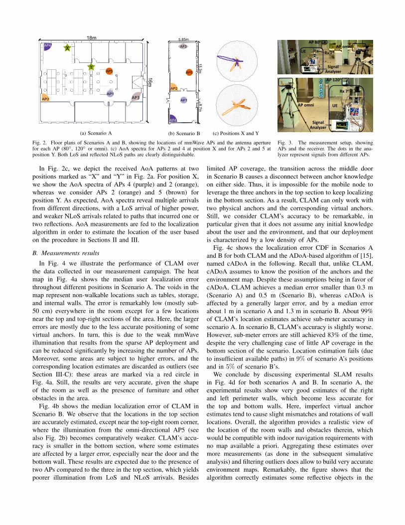
We use pseudo omni-directional transmitters in order tospeed up the collection of the measurements, and capture allavailable paths of a given AP at the same time. As a generalrule-of-thumb, we equipped APs located in open areas withan omni-directional antenna; where omni-directionality is notneeded we employed wide-beam antennas (e.g., 80◦-aperturehorn antennas for APs near corners, and open wave-guideterminations translating into a 120◦ antenna aperture for APslocated near walls).

Once the measurements have been collected at differentlocations, we retrieve the AoA patterns for each AP. Differentpeaks in each pattern correspond to the LoS arrival (whenavailable) and to one or more NLoS arrivals.

A. Room Setup

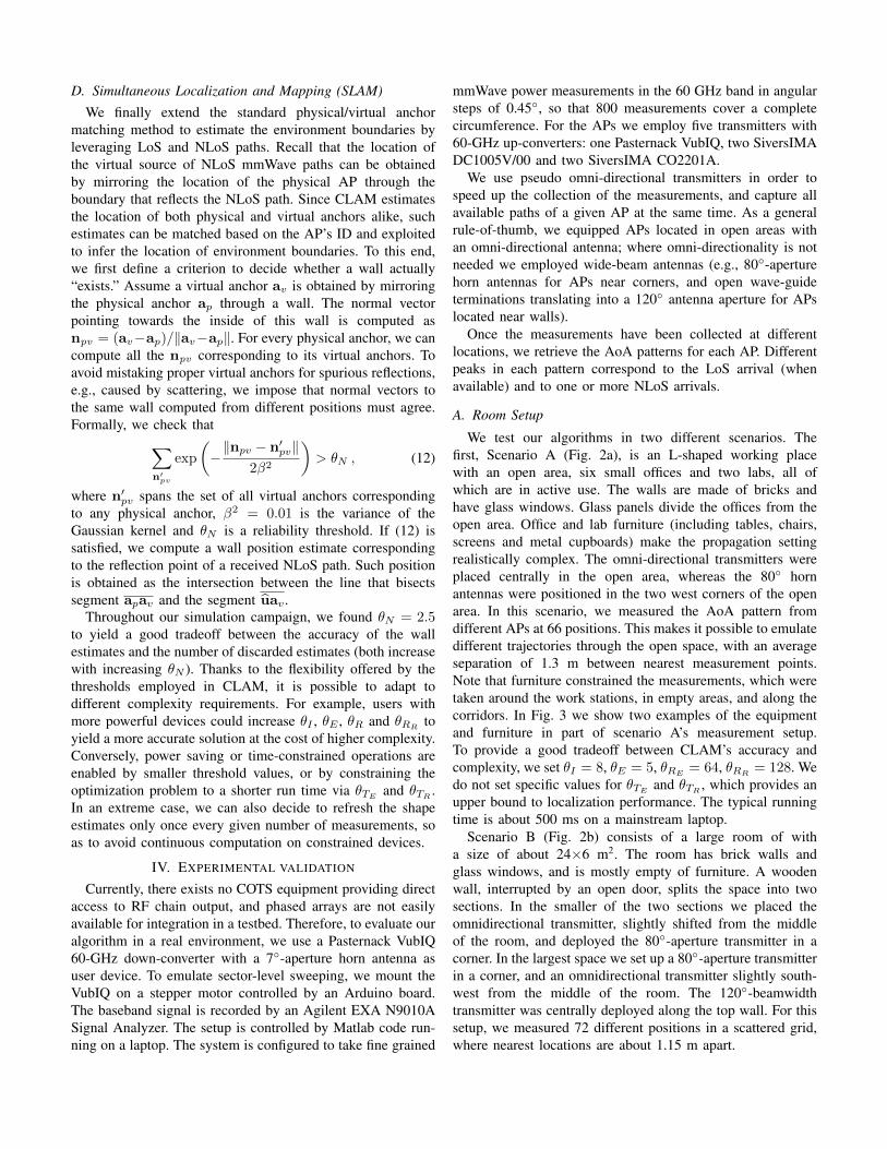
We test our algorithms in two different scenarios. Thefirst, Scenario A (Fig. 2a), is an L-shaped working placewith an open area, six small offices and two labs, all ofwhich are in active use. The walls are made of bricks andhave glass windows. Glass panels divide the offices from theopen area. Office and lab furniture (including tables, chairs,screens and metal cupboards) make the propagation settingrealistically complex. The omni-directional transmitters wereplaced centrally in the open area, whereas the 80◦ hornantennas were positioned in the two west corners of the openarea. In this scenario, we measured the AoA pattern fromdifferent APs at 66 positions. This makes it possible to emulatedifferent trajectories through the open space, with an averageseparation of 1.3 m between nearest measurement points.Note that furniture constrained the measurements, which weretaken around the work stations, in empty areas, and along thecorridors. In Fig. 3 we show two examples of the equipmentand furniture in part of scenario A’s measurement setup.To provide a good tradeoff between CLAM’s accuracy andcomplexity, we set θI = 8, θE = 5, θRE = 64, θRR = 128. Wedo not set specific values for θTE and θTR , which provides anupper bound to localization performance. The typical runningtime is about 500 ms on a mainstream laptop.

Scenario B (Fig. 2b) consists of a large room of witha size of about 24×6 m2. The room has brick walls andglass windows, and is mostly empty of furniture. A woodenwall, interrupted by an open door, splits the space into twosections. In the smaller of the two sections we placed theomnidirectional transmitter, slightly shifted from the middleof the room, and deployed the 80◦-aperture transmitter in acorner. In the largest space we set up a 80◦-aperture transmitterin a corner, and an omnidirectional transmitter slightly south-west from the middle of the room. The 120◦-beamwidthtransmitter was centrally deployed along the top wall. For thissetup, we measured 72 different positions in a scattered grid,where nearest locations are about 1.15 m apart.

AP5

X

Y

(a) Scenario A (b) Scenario B (c) Positions X and Y

Fig. 2. Floor plans of Scenarios A and B, showing the locations of mmWave APs and the antenna aperturefor each AP (80◦, 120◦ or omni). (c) AoA spectra for APs 2 and 4 at position X and for APs 2 and 5 atposition Y. Both LoS and reflected NLoS paths are clearly distinguishable.

AP 80°AP omni

UE Rx 7°

SignalAnalyzer

AP omni

AP 120°

Rx 7°

SignalAnalyzer

UE

Fig. 3. The measurement setup, showingAPs and the receiver. The dots in the ana-lyzer represent signals from different APs.

In Fig. 2c, we depict the received AoA patterns at twopositions marked as “X” and “Y” in Fig. 2a. For position X,we show the AoA spectra of APs 4 (purple) and 2 (orange),whereas we consider APs 2 (orange) and 5 (brown) forposition Y. As expected, AoA spectra reveal multiple arrivalsfrom different directions, with a LoS arrival of higher power,and weaker NLoS arrivals related to paths that incurred one ortwo reflections. AoA measurements are fed to the localizationalgorithm in order to estimate the location of the user basedon the procedure in Sections II and III.

B. Measurements results

In Fig. 4 we illustrate the performance of CLAM overthe data collected in our measurement campaign. The heatmap in Fig. 4a shows the median user localization errorthroughout different positions in Scenario A. The voids in themap represent non-walkable locations such as tables, storage,and internal walls. The error is remarkably low (mostly sub-50 cm) everywhere in the room except for a few locationsnear the top and top-right sections of the area. Here, the largererrors are mostly due to the less accurate positioning of somevirtual anchors. In turn, this is due to the weak mmWaveillumination that results from the sparse AP deployment andcan be reduced significantly by increasing the number of APs.Moreover, some areas are subject to higher errors, and thecorresponding location estimates are discarded as outliers (seeSection III-C): these areas are marked via a red circle inFig. 4a. Still, the results are very accurate, given the shapeof the room as well as the presence of furniture and otherobstacles in the area.

Fig. 4b shows the median localization error of CLAM inScenario B. We observe that the locations in the top sectionare accurately estimated, except near the top-right room corner,where the illumination from the omni-directional AP5 (seealso Fig. 2b) becomes comparatively weaker. CLAM’s accu-racy is smaller in the bottom section, where some estimatesare affected by a larger error, especially near the door and thebottom wall. These results are expected due to the presence oftwo APs compared to the three in the top section, which yieldspoorer illumination from LoS and NLoS arrivals. Besides

limited AP coverage, the transition across the middle doorin Scenario B causes a disconnect between anchor knowledgeon either side. Thus, it is impossible for the mobile node toleverage the three anchors in the top section to keep localizingin the bottom section. As a result, CLAM can only work withtwo physical anchors and the corresponding virtual anchors.Still, we consider CLAM’s accuracy to be remarkable, inparticular given that it does not assume any initial knowledgeabout the user and the environment, and that our deploymentis characterized by a low density of APs.

Fig. 4c shows the localization error CDF in Scenarios Aand B for both CLAM and the ADoA-based algorithm of [15],named cADoA in the following. Recall that, unlike CLAM,cADoA assumes to know the position of the anchors and theenvironment map. Despite these assumptions being in favor ofcADoA, CLAM achieves a median error smaller than 0.3 m(Scenario A) and 0.5 m (Scenario B), whereas cADoA isaffected by a generally larger error, and by a median errorabout 1 m in scenario A and 1.3 m in scenario B. About 99%of CLAM’s location estimates achieve sub-meter accuracy inscenario A. In scenario B, CLAM’s accuracy is slightly worse.However, sub-meter errors are still achieved 83% of the time,despite the very challenging case of little AP coverage in thebottom section of the scenario. Location estimation fails (dueto insufficient available paths) in 9% of scenario A’s positionsand in 5% of scenario B’s.

We conclude by discussing experimental SLAM resultsin Fig. 4d for both scenarios A and B. In scenario A, theexperimental results show very good estimates of the rightand left perimeter walls, which become less accurate forthe top and bottom walls. Here, imperfect virtual anchorestimates tend to cause slight mismatches and rotations of walllocations. Overall, the algorithm provides a realistic view ofthe location of the room walls and obstacles therein, whichwould be compatible with indoor navigation requirements withno map available a priori. Aggregating these estimates overmore measurements (as done in the subsequent simulativeanalysis) and filtering outliers does allow to build very accurateenvironment maps. Remarkably, the figure shows that thealgorithm correctly estimates some reflective objects in the

(a) Scenario A (b) Scenario B

0 0.2 0.4 0.6 0.8 1 1.2 1.4 1.6 1.8 2

Localization error x [m]

0

0.1

0.2

0.3

0.4

0.5

0.6

0.7

0.8

0.9

1

P(L

ocaliz

ation

err

or

< x)

Scenario A - CLAM

Scenario A - cADoA

Scenario B - CLAM

Scenario B - cADoA

(c) Error CDF (d) SLAM, scenarios A and B

Fig. 4. Experimental results for CLAM: heat maps of the median localization error for (a) scenario A and (b) scenario B; (c) CDF of the localization error.(d) Experimental SLAM results for scenarios A and B: gray lines represent the walls, and each dot a wall location estimate.

open area at the time of the measurement, including screensin the second table from the top.

The SLAM performance is comparatively worse in sce-nario B, where CLAM correctly estimates the right perimeterwall, together with the top and middle walls, and a fewlocations in the bottom wall. The left wall is affected by ahigher uncertainty, as only a few marked points appear. Still,given the challenging scenario with only a few APs and thefact that environmental sensing comes as an added value ofthe localization algorithm, we believe these results to be verypromising and worth further investigation.

V. SIMULATION RESULTS

To investigate CLAM’s performance in more detail, we nowreproduce scenarios A and B of Section IV in simulation.We use a custom ray-tracing based simulator that accuratelymodels the propagation environment, and solves the electro-magnetic propagation equations by taking into account theproperties of the different materials that constitute the wallsand other objects in the scenarios. This allows us to emulatemany user trajectories (something that would be too time-consuming in a real measurement), to systematically evaluatemutual mmWave path blockage by the users, and to understandthe long-term performance of CLAM when the movement ofthe user through the environment enables continued refinementof position estimates over time.

With reference to Figs. 5a and 5b, in each scenario wedeploy five physical APs (large stars, where smaller starsrepresent their virtual counterparts). We consider a total offive users that move along a smooth trajectory at 1 m/s. Thetrajectories are rendered using light purple lines and points.The green path is one example path we highlight to discuss thelocalization results below. Each node takes AoA measurementsat different locations (marked with dots for the purple paths,or circles for the green path), and applies CLAM to locatethe physical and virtual anchor nodes, and to estimate its ownposition while moving. We simulate the mutual blockage ofmmWave paths by modeling the users as circles of diameter0.6 m, and by assuming that any path crossing such circlesdoes not propagate further. For any given user, between 20%and 25% of the propagation paths are blocked throughoutscenario A, and between 15% and 20% in scenario B.

We start with Fig. 6 for scenario A and Fig. 7 for scenarioB, which show the cumulative distribution function (CDF)of the user localization error, computed over the ensembleof location estimates taken by all mobile users. CLAM iscompared to the two approaches in [15], which belong tothe class of triangulation-based and ADoA-based algorithms,respectively named cTV and cADoA. Unlike CLAM, bothcTV and cADoA assume to know the position of the anchorsand the floor map, so as to be able to locate virtual anchors.All schemes are tested by assuming angle measurements tobe affected by a Gaussian error of standard deviation σ = 1◦

and σ = 2◦. These errors correspond to those obtained bysynthesizing beam shapes with a uniform linear array with 32and 16 elements, respectively, under typical SNR conditions.

We observe that CLAM achieves much smaller localizationerrors than cTV and cADoA, despite starting with zero initialknowledge about the AP locations and the environment. In sce-nario A, up to 97% of the location estimates are affected by anerror of less than 50 cm, with a median error between 10 and20 cm, depending on the accuracy of the AoA measurements.cADoA and cTV perform worse, especially if AoA data isless accurate (σ = 2◦). CLAM fails to localize a user between0.5% and 1.5% of the time3, against 0.06% for cADoA andno failures for cTV. Scenario B (Fig. 7) shows the sametrend. However, the inner wall makes the anchor configurationsparser, and increases the probability that users block mmWavepaths through the door. This is reflected by CLAM beingslightly less accurate than in scenario A. In any event, it stillachieves sub-meter accuracy (about 95% of the cases) anda median error of about 15 cm for σ = 1◦. We observe thatcADoA and cTV show much larger median and average errors,and a significant probability that the localization error exceeds2 m for less accurate angle measurements. In scenario B, thepercentage of localization failures is between 2% and 4% forCLAM (no failures for cADoA and cTV). We note that if weapplied the outlier detection filter to cADoA and cTV, theirlack of accuracy would lead to discarding up to 20% of theestimates for scenario A and up to 30% for scenario B.

We now focus on the trajectory of a single user (the greenpath in Figs. 5a and 5b), in order to investigate the localization

3Failure occurs when a point is not illuminated by a sufficient number ofanchors, or because an estimate is marked as an outlier as per Section III-C.

0 4 8 12 16

x-axis location [m]

0

4

8

12

16

y-a

xis

location [m

]

Example path

Other paths

Walls

AP

V. anchor

Location est.

Anchors est.

(a) Scenario A

0 4

x-axis location [m]

0

4

8

12

16

20

24

y-a

xis

lo

ca

tio

n [

m]

(b) Scenario B

Fig. 5. Simulations: localization results for scenarios A and B. Localizationis quite accurate despite mutual mmWave path blockage among the users.

errors in more detail. Recall that large stars correspond tophysical APs, whereas small stars represent virtual APs, thatmodel the (virtual) sources of NLoS paths. The uncertainty ofanchor and user location estimates is rendered through ellipseswhose half-axis lengths equate the standard deviation of theestimation error along the corresponding direction. Most of theestimated anchor and user locations are extremely accurate,as seen from the tiny uncertainty contours. This includes allphysical and almost all virtual anchors. Just for those anchorsthat the user observes only from a few positions do theuncertainty ellipses become larger.

As a general observation, if some anchor position estimatesare affected by higher uncertainty, the user location estimatesrelying on those anchors will be less accurate as well. Thiscan be observed in the bottom section of scenario B (Fig. 5b).The frequent mmWave propagation path blockage due to otherusers limits the number of anchor observations in the bottomsection, which translates into lower accuracy. At the sametime, users block the visibility of the anchors in either roomas they move through the door, which prevents leveraginginformation from both anchor sets. In the larger section, pathblockage is mitigated due to the larger room space, whichleads to more accurate location estimates.

We finally show in Fig. 8 the results of the estimation ofroom walls and obstacles via the SLAM algorithm describedin Section III-D. Fig. 8a shows that SLAM works well inscenario A: the location of all walls is estimated with goodaccuracy, with only a few spurious results. Those are mainlydue to the error in the position estimate of some physicaland virtual anchors (see Fig. 5a) near the top wall and nearthe internal wall in the bottom part of the room. The lackof estimates for the bottom right part, instead, is due to aninsufficient number of physical-virtual anchor pairs that agreeon the existence of a wall, so that (12) does not exceed thethreshold θN . In scenario B the results are good as well. Giventhe slightly higher localization errors, a few walls are estimatedwith the wrong inclination, especially in the bottom section.We remark that SLAM results in both scenarios would become

0 0.2 0.4 0.6 0.8 1 1.2 1.4 1.6 1.8 2

Localization error x [m]

0

0.1

0.2

0.3

0.4

0.5

0.6

0.7

0.8

0.9

1

P(L

oca

liza

tion

err

or

< x

)

=1

=2

CLAM

cTV

cADoA

Fig. 6. Simulations: localization er-ror CDF for scenario A.

Fig. 7. Simulations: localization er-ror CDF for scenario B.

(a) Scenario A. (b) Scenario B

Fig. 8. SLAM simulation results for (a) scenario A and (b) scenario B. Lightgray lines show the walls; each black dot represents a wall location estimate.

more accurate with a denser AP deployment, or by takingfurther measurements, e.g., as a user repeatedly walks throughthe respective indoor areas.

VI. RELATED WORK

The literature most related to our approach lies in the areasof localization and SLAM. We survey each category below.Localization in mmWave systems— Localization has beenlargely studied from theoretical and practical standpoints [18].Localization is considered as an inherent feature of mmWavecommunications [19], and thanks to the characteristics ofmmWave signals is potentially achievable with up to sub-centimeter accuracy. Large-scale mmWave MIMO systemshave been leveraged for localization by detecting the changesin the statistics of sparse MIMO channel signatures [20].From a theoretical standpoint, [21] shows that in a number ofpractical cases it is possible to estimate both the position andthe orientation of a user. This is in line with the capabilitiesof our proposed algorithm.

The quasi-optical propagation as well as the sparse AoAspectrum perceived by a mmWave receiver enable single-anchor localization, with much better accuracy than can beachieved in microwave systems [22], especially if the envi-ronment and the AP locations are assumed unknown. Forexample, [15] achieves this via two approaches belongingto the class of triangulation- and ADoA-based algorithms.In the same vein, [14] applies ranging and multilateration

to to exploit LoS and NLoS arrivals for node localization.The work in [16] is a first attempt to achieve localizationwithout initial knowledge of the environment. However, noexperimental results are provided.Simultaneous localization and mapping— SLAM is a funda-mental problem in the field of computer vision applied torobotics [23]. The original solution employed a laser rangescanner (or other range, bearing or odometry sensors) andfused the measurements via an extended Kalman filter (EKF).Laser or lidar scanning and depth cameras have then evolvedto GPU-based or cloud implementations [24] that reduce com-plexity by offloading computationally intensive tasks. A range-based algorithm that exploits accurate range measurements ina multipath environment was proposed for SLAM in [25].SLAM has also been realized through bearing-only sensors,often in conjunction with the EKF or other robust smoothingtechniques, such as Rao-Blackwellized particle filters [26].

Our CLAM algorithm achieves SLAM in mmWave net-works through ADoA information extracted from standard-compliant beam training and tracking algorithms. Unlike [14],[27] and to abide to COTS device constraints, we do notperform ranging, and unlike [15], [22] we assume no a-prioriinformation. Our algorithm is distributed and does not requirethe nodes to cooperate (unlike, e.g., [28]). Anchor locationsare estimated by exploiting all possible relationships amongthe angles measured by a client at different locations. Tothe best of the authors’ knowledge, it is the first time sucha formulation is used, enabling a high-accuracy and low-complexity implementation, including fast initialization.

VII. CONCLUSIONS

In this paper, we proposed CLAM, a zero-initial infor-mation, zero-overhead and low-complexity SLAM approachtailored to the characteristics of mmWave networks. Weleverage only standard procedures such as beam-training toretrieve angle-difference-of-arrival information, and use thisinformation to estimate the location of the mmWave APs, theposition of the user, and the surrounding environment. Low-complexity estimation procedures are enabled by a fundamen-tal reformulation of ADoA-based anchor location estimation.

We demonstrate that CLAM localizes with very high ac-curacy, and that it is robust to mmWave signal blockagedue to human movement in the localization area. Our resultsare based on extensive experimental measurements in twodifferent areas, including a fully operational working area,as well as additional simulations. The outcomes validate theaccuracy of CLAM and demonstrate that it is a feasibleapproach for realistic mmWave network deployments.

ACKNOWLEDGMENT

This work has been supported in part by the ERC projectSEARCHLIGHT, grant no. 617721, the Ramon y Cajal grantRYC-2012-10788, the grant TEC2014-55713-R (Hyperadapt)and the Madrid Regional Government through the TIGRE5-CM program (S2013/ICE-2919).

REFERENCES

[1] S. Rangan, T. Rappaport, and E. Erkip, “Millimeter-wave cellularwireless networks: Potentials and challenges,” Proceedings of the IEEE,vol. 102, no. 3, pp. 366–385, Mar. 2014.

[2] Z. Pi, J. Choi, and R. Heath, “Millimeter-wave gigabit broadbandevolution toward 5G: fixed access and backhaul,” IEEE Commun. Mag.,vol. 54, no. 4, pp. 138–144, Apr. 2016.

[3] TP-Link. Talon AD7200 multi-band WiFi router. [Online]. Available:http://www.tp-link.com/us/products/details/cat-5506 AD7200.html

[4] NETGEAR. Nighthawk X10 smart WiFi router. [Online]. Available:https://www.netgear.com/landings/ad7200/

[5] T. Rappaport et al., “Broadband millimeter-wave propagation measure-ments and models using adaptive-beam antennas for outdoor urbancellular communications,” IEEE Trans. Antennas Propag., vol. 61, no. 4,pp. 1850–1859, Apr. 2013.

[6] J. G. Andrews et al., “Modeling and analyzing millimeter wave cellularsystems,” IEEE Trans. Commun., vol. 65, no. 1, pp. 403–430, Jan. 2017.

[7] M. Giordani, M. Mezzavilla, and M. Zorzi, “Initial access in 5GmmWave cellular networks,” IEEE Commun. Mag., vol. 54, no. 11, pp.40–47, Nov. 2016.

[8] Y. Kim et al., “Feasibility of mobile cellular communications at mil-limeter wave frequency,” IEEE J. Sel. Topics Signal Process., vol. 10,no. 3, pp. 589–599, Apr. 2016.

[9] T. Nitsche et al., “IEEE 802.11ad: directional 60 ghz communication formulti-Gigabit-per-second Wi-Fi,” IEEE Commun. Mag., vol. 52, no. 12,pp. 132–141, Dec. 2014.

[10] M. E. Rasekh et al., “Noncoherent mmWave path tracking,” inProc. ACM HotMobile, Sonoma, CA, USA, Feb. 2017.

[11] S. Sur et al., “BeamSpy: Enabling robust 60 GHz links under blockage,”in Proc. USENIX NSDI, Santa Clara, CA, Mar. 2016.

[12] M. K. Haider and E. W. Knightly, “Mobility resilience and overheadconstrained adaptation in directional 60 GHz WLANs: Protocol designand system implementation,” in Proc. ACM MobiHoc, Paderborn, Ger-many, Jul. 2016.

[13] M. Simsek et al., “5G-enabled tactile internet,” IEEE J. Sel. AreasCommun., vol. 34, no. 3, pp. 460–473, Mar. 2016.

[14] J. Chen et al., “Pseudo lateration: Millimeter-wave localization using asingle RF chain,” in Proc. IEEE WCNC, San Francisco, CA, Mar. 2017.

[15] A. Olivier et al., “Lightweight indoor localization for 60-GHz millimeterwave systems,” in Proc. IEEE SECON, London, UK, Jun. 2016.

[16] J. Palacios, P. Casari, and J. Widmer, “JADE: Zero-knowledge devicelocalization and environment mapping for millimeter wave systems,” inProc. IEEE INFOCOM, Atlanta, GA, May 2017.

[17] J. C. Lagarias et al., “Convergence properties of the Nelder–Meadsimplex method in low dimensions,” SIAM Journal on Optimization,vol. 9, no. 1, pp. 112–147, 1998.

[18] J. Aspnes et al., “A theory of network localization,” IEEE Trans. MobileComput., vol. 5, no. 12, pp. 1663–1678, Dec. 2006.

[19] F. Lemic et al., “Localization as a feature of mmWave communication,”in Proc. IWCMC, Paphos, Cyprus, Sep. 2016.

[20] H. Deng and A. Sayeed, “Mm-wave MIMO channel modeling and userlocalization using sparse beamspace signatures,” in Proc. IEEE SPAWC,Toronto, Canada, Jun. 2014.

[21] A. Shahmansoori et al., “5G position and orientation estimation throughmillimeter wave MIMO,” in Proc. IEEE GlobeCom, Dec. 2015.

[22] P. Meissner et al., “Accurate and robust indoor localization systems usingultra-wideband signals,” in Proc. ENC, Vienna, Austria, Apr. 2012.

[23] C. Cadena et al., “Past, present, and future of simultaneous localizationand mapping: Toward the robust-perception age,” IEEE Trans. Robot.,vol. 32, no. 6, pp. 1309–1332, Dec. 2016.

[24] S. Dey and A. Mukherjee, “Robotic SLAM: A review from fog comput-ing and mobile edge computing perspective,” in Proc. MOBIQUITOUS,Hiroshima, Japan, Nov. 2016.

[25] H. Naseri and V. Koivunen, “Cooperative simultaneous localizationand mapping by exploiting multipath propagation,” IEEE Trans. SignalProcess., vol. 65, no. 1, pp. 200–211, Jan. 2017.

[26] M. Deans and M. Hebert, Experimental comparison of techniques forlocalization and mapping using a bearing-only sensor. Springer BerlinHeidelberg, 2001, pp. 395–404.

[27] D. Moore et al., “Robust distributed network localization with noisyrange measurements,” in Proc. ACM SenSys, Baltimore, MD, Nov. 2004.

[28] J. Xu, M. Ma, and C. L. Law, “AoA cooperative position localization,”in Proc. IEEE GLOBECOM, New Orleans, LA, Nov. 2008.