communications and control engineering - doc.lagout.org science/2_algorithms... · sergio bittanti...
TRANSCRIPT


Communications and Control Engineering
For other titles published in this series, go towww.springer.com/series/61


Series EditorsA. Isidori � J.H. van Schuppen � E.D. Sontag � M. Thoma � M. Krstic
Published titles include:Stability and Stabilization of Infinite DimensionalSystems with ApplicationsZheng-Hua Luo, Bao-Zhu Guo and Omer Morgul
Nonsmooth Mechanics (Second edition)Bernard Brogliato
Nonlinear Control Systems IIAlberto Isidori
L2-Gain and Passivity Techniques in Nonlinear ControlArjan van der Schaft
Control of Linear Systems with Regulation and InputConstraintsAli Saberi, Anton A. Stoorvogel and PeddapullaiahSannuti
Robust and H∞ ControlBen M. Chen
Computer Controlled SystemsEfim N. Rosenwasser and Bernhard P. Lampe
Control of Complex and Uncertain SystemsStanislav V. Emelyanov and Sergey K. Korovin
Robust Control Design Using H∞ MethodsIan R. Petersen, Valery A. Ugrinovski andAndrey V. Savkin
Model Reduction for Control System DesignGoro Obinata and Brian D.O. Anderson
Control Theory for Linear SystemsHarry L. Trentelman, Anton Stoorvogel and Malo Hautus
Functional Adaptive ControlSimon G. Fabri and Visakan Kadirkamanathan
Positive 1D and 2D SystemsTadeusz Kaczorek
Identification and Control Using Volterra ModelsFrancis J. Doyle III, Ronald K. Pearson and BabatundeA. Ogunnaike
Non-linear Control for Underactuated MechanicalSystemsIsabelle Fantoni and Rogelio Lozano
Robust Control (Second edition)Jürgen Ackermann
Flow Control by FeedbackOle Morten Aamo and Miroslav Krstic
Learning and Generalization (Second edition)Mathukumalli Vidyasagar
Constrained Control and EstimationGraham C. Goodwin, Maria M. Seron andJosé A. De Doná
Randomized Algorithms for Analysis and Controlof Uncertain SystemsRoberto Tempo, Giuseppe Calafiore and FabrizioDabbene
Switched Linear SystemsZhendong Sun and Shuzhi S. Ge
Subspace Methods for System IdentificationTohru Katayama
Digital Control SystemsIoan D. Landau and Gianluca Zito
Multivariable Computer-controlled SystemsEfim N. Rosenwasser and Bernhard P. Lampe
Dissipative Systems Analysis and Control(Second edition)Bernard Brogliato, Rogelio Lozano, Bernhard Maschkeand Olav Egeland
Algebraic Methods for Nonlinear Control SystemsGiuseppe Conte, Claude H. Moog and Anna M. Perdon
Polynomial and Rational MatricesTadeusz Kaczorek
Simulation-based Algorithms for Markov DecisionProcessesHyeong Soo Chang, Michael C. Fu, Jiaqiao Hu andSteven I. Marcus
Iterative Learning ControlHyo-Sung Ahn, Kevin L. Moore and YangQuan Chen
Distributed Consensus in Multi-vehicle CooperativeControlWei Ren and Randal W. Beard
Control of Singular Systems with Random AbruptChangesEl-Kébir Boukas
Nonlinear and Adaptive Control with ApplicationsAlessandro Astolfi, Dimitrios Karagiannis and RomeoOrtega
Stabilization, Optimal and Robust ControlAziz Belmiloudi
Control of Nonlinear Dynamical SystemsFelix L. Chernous’ko, Igor M. Ananievski and SergeyA. Reshmin
Periodic SystemsSergio Bittanti and Patrizio Colaneri
Discontinuous SystemsYury V. Orlov
Constructions of Strict Lyapunov FunctionsMichael Malisoff and Frédéric Mazenc
Controlling ChaosHuaguang Zhang, Derong Liu and Zhiliang Wang
Stabilization of Navier–Stokes FlowsViorel Barbu
Distributed Control of Multi-agent NetworksWei Ren and Yongcan Cao

Lars Grüne � Jürgen Pannek
Nonlinear ModelPredictive Control
Theory and Algorithms

Lars GrüneMathematisches InstitutUniversität BayreuthBayreuth [email protected]
Jürgen PannekMathematisches InstitutUniversität BayreuthBayreuth [email protected]
ISSN 0178-5354ISBN 978-0-85729-500-2 e-ISBN 978-0-85729-501-9DOI 10.1007/978-0-85729-501-9Springer London Dordrecht Heidelberg New York
British Library Cataloguing in Publication DataA catalogue record for this book is available from the British Library
Library of Congress Control Number: 2011926502
Mathematics Subject Classification (2010): 93-02, 92C10, 93D15, 49M37
© Springer-Verlag London Limited 2011Apart from any fair dealing for the purposes of research or private study, or criticism or review, as per-mitted under the Copyright, Designs and Patents Act 1988, this publication may only be reproduced,stored or transmitted, in any form or by any means, with the prior permission in writing of the publish-ers, or in the case of reprographic reproduction in accordance with the terms of licenses issued by theCopyright Licensing Agency. Enquiries concerning reproduction outside those terms should be sent tothe publishers.The use of registered names, trademarks, etc., in this publication does not imply, even in the absence of aspecific statement, that such names are exempt from the relevant laws and regulations and therefore freefor general use.The publisher makes no representation, express or implied, with regard to the accuracy of the informationcontained in this book and cannot accept any legal responsibility or liability for any errors or omissionsthat may be made.
Cover design: VTeX UAB, Lithuania
Printed on acid-free paper
Springer is part of Springer Science+Business Media (www.springer.com)

For Brigitte, Florian and CarlaLG
For Sabina and AlinaJP

Preface
The idea for this book grew out of a course given at a winter school of the In-ternational Doctoral Program “Identification, Optimization and Control with Ap-plications in Modern Technologies” in Schloss Thurnau in March 2009. Initially,the main purpose of this course was to present results on stability and performanceanalysis of nonlinear model predictive control algorithms, which had at that timerecently been obtained by ourselves and coauthors. However, we soon realized thatboth the course and even more the book would be inevitably incomplete withouta comprehensive coverage of classical results in the area of nonlinear model pre-dictive control and without the discussion of important topics beyond stability andperformance, like feasibility, robustness, and numerical methods.
As a result, this book has become a mixture between a research monograph andan advanced textbook. On the one hand, the book presents original research resultsobtained by ourselves and coauthors during the last five years in a comprehensiveand self contained way. On the other hand, the book also presents a number ofresults—both classical and more recent—of other authors. Furthermore, we haveincluded a lot of background information from mathematical systems theory, op-timal control, numerical analysis and optimization to make the book accessible tograduate students—on PhD and Master level—from applied mathematics and con-trol engineering alike. Finally, via our web page www.nmpc-book.com we provideMATLAB and C++ software for all examples in this book, which enables the readerto perform his or her own numerical experiments. For reading this book, we assumea basic familiarity with control systems, their state space representation as well aswith concepts like feedback and stability as provided, e.g., in undergraduate courseson control engineering or in courses on mathematical systems and control theory inan applied mathematics curriculum. However, no particular knowledge of nonlin-ear systems theory is assumed. Substantial parts of the systems theoretic chaptersof the book have been used by us for a lecture on nonlinear model predictive con-trol for master students in applied mathematics and we believe that the book is wellsuited for this purpose. More advanced concepts like time varying formulations orpeculiarities of sampled data systems can be easily skipped if only time invariantproblems or discrete time systems shall be treated.
vii

viii Preface
The book centers around two main topics: systems theoretic properties of nonlin-ear model predictive control schemes on the one hand and numerical algorithms onthe other hand; for a comprehensive description of the contents we refer to Sect. 1.3.As such, the book is somewhat more theoretical than engineering or application ori-ented monographs on nonlinear model predictive control, which are furthermoreoften focused on linear methods.
Within the nonlinear model predictive control literature, distinctive features ofthis book are the comprehensive treatment of schemes without stabilizing terminalconstraints and the in depth discussion of performance issues via infinite horizonsuboptimality estimates, both with and without stabilizing terminal constraints. Thekey for the analysis in the systems theoretic part of this book is a uniform wayof interpreting both classes of schemes as relaxed versions of infinite horizon op-timal control problems. The relaxed dynamic programming framework developedin Chap. 4 is thus a cornerstone of this book, even though we do not use dynamicprogramming for actually solving nonlinear model predictive control problems; forthis task we prefer direct optimization methods as described in the last chapter ofthis book, since they also allow for the numerical treatment of high dimensionalsystems.
There are many people whom we have to thank for their help in one or the otherway. For pleasant and fruitful collaboration within joint research projects and onjoint papers—of which many have been used as the basis for this book—we aregrateful to Frank Allgöwer, Nils Altmüller, Rolf Findeisen, Marcus von Lossow,Dragan Nešic, Anders Rantzer, Martin Seehafer, Paolo Varutti and Karl Worthmann.For enlightening talks, inspiring discussions, for organizing workshops and mini-symposia (and inviting us) and, last but not least, for pointing out valuable referencesto the literature we would like to thank David Angeli, Moritz Diehl, Knut Graichen,Peter Hokayem, Achim Ilchmann, Andreas Kugi, Daniel Limón, Jan Lunze, LaloMagni, Manfred Morari, Davide Raimondo, Saša Rakovic, Jörg Rambau, Jim Rawl-ings, Markus Reble, Oana Serea and Andy Teel, and we apologize to everyone whois missing in this list although he or she should have been mentioned. Without theproof reading of Nils Altmüller, Robert Baier, Thomas Jahn, Marcus von Lossow,Florian Müller and Karl Worthmann the book would contain even more typos andinaccuracies than it probably does—of course, the responsibility for all remainingerrors lies entirely with us and we appreciate all comments on errors, typos, miss-ing references and the like. Beyond proof reading, we are grateful to Thomas Jahnfor his help with writing the software supporting this book and to Karl Worthmannfor his contributions to many results in Chaps. 6 and 7, most importantly the proofof Proposition 6.17. Finally, we would like to thank Oliver Jackson and CharlotteCross from Springer-Verlag for their excellent support.
Lars GrüneJürgen Pannek
Bayreuth, GermanyApril 2011
Contents
1 Introduction . . . . . . . . . . . . . . . . . . . . . . . . . . . . . . . . 11.1 What Is Nonlinear Model Predictive Control? . . . . . . . . . . . 11.2 Where Did NMPC Come from? . . . . . . . . . . . . . . . . . . . 31.3 How Is This Book Organized? . . . . . . . . . . . . . . . . . . . . 51.4 What Is Not Covered in This Book? . . . . . . . . . . . . . . . . . 9
References . . . . . . . . . . . . . . . . . . . . . . . . . . . . . . 10
2 Discrete Time and Sampled Data Systems . . . . . . . . . . . . . . . 132.1 Discrete Time Systems . . . . . . . . . . . . . . . . . . . . . . . . 132.2 Sampled Data Systems . . . . . . . . . . . . . . . . . . . . . . . . 162.3 Stability of Discrete Time Systems . . . . . . . . . . . . . . . . . 282.4 Stability of Sampled Data Systems . . . . . . . . . . . . . . . . . 352.5 Notes and Extensions . . . . . . . . . . . . . . . . . . . . . . . . 392.6 Problems . . . . . . . . . . . . . . . . . . . . . . . . . . . . . . . 39
References . . . . . . . . . . . . . . . . . . . . . . . . . . . . . . 41
3 Nonlinear Model Predictive Control . . . . . . . . . . . . . . . . . . 433.1 The Basic NMPC Algorithm . . . . . . . . . . . . . . . . . . . . 433.2 Constraints . . . . . . . . . . . . . . . . . . . . . . . . . . . . . . 453.3 Variants of the Basic NMPC Algorithms . . . . . . . . . . . . . . 503.4 The Dynamic Programming Principle . . . . . . . . . . . . . . . . 563.5 Notes and Extensions . . . . . . . . . . . . . . . . . . . . . . . . 623.6 Problems . . . . . . . . . . . . . . . . . . . . . . . . . . . . . . . 64
References . . . . . . . . . . . . . . . . . . . . . . . . . . . . . . 65
4 Infinite Horizon Optimal Control . . . . . . . . . . . . . . . . . . . . 674.1 Definition and Well Posedness of the Problem . . . . . . . . . . . 674.2 The Dynamic Programming Principle . . . . . . . . . . . . . . . . 704.3 Relaxed Dynamic Programming . . . . . . . . . . . . . . . . . . . 754.4 Notes and Extensions . . . . . . . . . . . . . . . . . . . . . . . . 814.5 Problems . . . . . . . . . . . . . . . . . . . . . . . . . . . . . . . 83
References . . . . . . . . . . . . . . . . . . . . . . . . . . . . . . 84
ix

x Contents
5 Stability and Suboptimality Using Stabilizing Constraints . . . . . . 875.1 The Relaxed Dynamic Programming Approach . . . . . . . . . . . 875.2 Equilibrium Endpoint Constraint . . . . . . . . . . . . . . . . . . 885.3 Lyapunov Function Terminal Cost . . . . . . . . . . . . . . . . . . 955.4 Suboptimality and Inverse Optimality . . . . . . . . . . . . . . . . 1015.5 Notes and Extensions . . . . . . . . . . . . . . . . . . . . . . . . 1095.6 Problems . . . . . . . . . . . . . . . . . . . . . . . . . . . . . . . 110
References . . . . . . . . . . . . . . . . . . . . . . . . . . . . . . 112
6 Stability and Suboptimality Without Stabilizing Constraints . . . . . 1136.1 Setting and Preliminaries . . . . . . . . . . . . . . . . . . . . . . 1136.2 Asymptotic Controllability with Respect to � . . . . . . . . . . . . 1166.3 Implications of the Controllability Assumption . . . . . . . . . . . 1196.4 Computation of α . . . . . . . . . . . . . . . . . . . . . . . . . . 1216.5 Main Stability and Performance Results . . . . . . . . . . . . . . . 1256.6 Design of Good Running Costs � . . . . . . . . . . . . . . . . . . 1336.7 Semiglobal and Practical Asymptotic Stability . . . . . . . . . . . 1426.8 Proof of Proposition 6.17 . . . . . . . . . . . . . . . . . . . . . . 1506.9 Notes and Extensions . . . . . . . . . . . . . . . . . . . . . . . . 1596.10 Problems . . . . . . . . . . . . . . . . . . . . . . . . . . . . . . . 161
References . . . . . . . . . . . . . . . . . . . . . . . . . . . . . . 162
7 Variants and Extensions . . . . . . . . . . . . . . . . . . . . . . . . . 1657.1 Mixed Constrained–Unconstrained Schemes . . . . . . . . . . . . 1657.2 Unconstrained NMPC with Terminal Weights . . . . . . . . . . . 1687.3 Nonpositive Definite Running Cost . . . . . . . . . . . . . . . . . 1707.4 Multistep NMPC-Feedback Laws . . . . . . . . . . . . . . . . . . 1747.5 Fast Sampling . . . . . . . . . . . . . . . . . . . . . . . . . . . . 1767.6 Compensation of Computation Times . . . . . . . . . . . . . . . . 1807.7 Online Measurement of α . . . . . . . . . . . . . . . . . . . . . . 1837.8 Adaptive Optimization Horizon . . . . . . . . . . . . . . . . . . . 1917.9 Nonoptimal NMPC . . . . . . . . . . . . . . . . . . . . . . . . . 1987.10 Beyond Stabilization and Tracking . . . . . . . . . . . . . . . . . 207
References . . . . . . . . . . . . . . . . . . . . . . . . . . . . . . 209
8 Feasibility and Robustness . . . . . . . . . . . . . . . . . . . . . . . . 2118.1 The Feasibility Problem . . . . . . . . . . . . . . . . . . . . . . . 2118.2 Feasibility of Unconstrained NMPC Using Exit Sets . . . . . . . . 2148.3 Feasibility of Unconstrained NMPC Using Stability . . . . . . . . 2178.4 Comparing Terminal Constrained vs. Unconstrained NMPC . . . . 2228.5 Robustness: Basic Definition and Concepts . . . . . . . . . . . . . 2258.6 Robustness Without State Constraints . . . . . . . . . . . . . . . . 2278.7 Examples for Nonrobustness Under State Constraints . . . . . . . 2328.8 Robustness with State Constraints via Robust-optimal Feasibility . 2378.9 Robustness with State Constraints via Continuity of VN . . . . . . 2418.10 Notes and Extensions . . . . . . . . . . . . . . . . . . . . . . . . 2468.11 Problems . . . . . . . . . . . . . . . . . . . . . . . . . . . . . . . 249
References . . . . . . . . . . . . . . . . . . . . . . . . . . . . . . 249

Contents xi
9 Numerical Discretization . . . . . . . . . . . . . . . . . . . . . . . . . 2519.1 Basic Solution Methods . . . . . . . . . . . . . . . . . . . . . . . 2519.2 Convergence Theory . . . . . . . . . . . . . . . . . . . . . . . . . 2569.3 Adaptive Step Size Control . . . . . . . . . . . . . . . . . . . . . 2609.4 Using the Methods Within the NMPC Algorithms . . . . . . . . . 2649.5 Numerical Approximation Errors and Stability . . . . . . . . . . . 2669.6 Notes and Extensions . . . . . . . . . . . . . . . . . . . . . . . . 2699.7 Problems . . . . . . . . . . . . . . . . . . . . . . . . . . . . . . . 271
References . . . . . . . . . . . . . . . . . . . . . . . . . . . . . . 272
10 Numerical Optimal Control of Nonlinear Systems . . . . . . . . . . . 27510.1 Discretization of the NMPC Problem . . . . . . . . . . . . . . . . 27510.2 Unconstrained Optimization . . . . . . . . . . . . . . . . . . . . . 28810.3 Constrained Optimization . . . . . . . . . . . . . . . . . . . . . . 29210.4 Implementation Issues in NMPC . . . . . . . . . . . . . . . . . . 31510.5 Warm Start of the NMPC Optimization . . . . . . . . . . . . . . . 32410.6 Nonoptimal NMPC . . . . . . . . . . . . . . . . . . . . . . . . . 33110.7 Notes and Extensions . . . . . . . . . . . . . . . . . . . . . . . . 33510.8 Problems . . . . . . . . . . . . . . . . . . . . . . . . . . . . . . . 337
References . . . . . . . . . . . . . . . . . . . . . . . . . . . . . . 337
Appendix NMPC Software Supporting This Book . . . . . . . . . . . . 341A.1 The MATLAB NMPC Routine . . . . . . . . . . . . . . . . . . . 341A.2 Additional MATLAB and MAPLE Routines . . . . . . . . . . . . 343A.3 The C++ NMPC Software . . . . . . . . . . . . . . . . . . . . . . 345
Glossary . . . . . . . . . . . . . . . . . . . . . . . . . . . . . . . . . . . . 347
Index . . . . . . . . . . . . . . . . . . . . . . . . . . . . . . . . . . . . . . 353

Chapter 1Introduction
1.1 What Is Nonlinear Model Predictive Control?
Nonlinear model predictive control (henceforth abbreviated as NMPC) is an opti-mization based method for the feedback control of nonlinear systems. Its primaryapplications are stabilization and tracking problems, which we briefly introduce inorder to describe the basic idea of model predictive control.
Suppose we are given a controlled process whose state x(n) is measured at dis-crete time instants tn, n = 0,1,2, . . . . “Controlled” means that at each time instantwe can select a control input u(n) which influences the future behavior of the stateof the system. In tracking control, the task is to determine the control inputs u(n)
such that x(n) follows a given reference xref(n) as good as possible. This means thatif the current state is far away from the reference then we want to control the systemtowards the reference and if the current state is already close to the reference thenwe want to keep it there. In order to keep this introduction technically simple, weconsider x(n) ∈ X = R
d and u(n) ∈ U = Rm, furthermore we consider a reference
which is constant and equal to x∗ = 0, i.e., xref(n) = x∗ = 0 for all n ≥ 0. With sucha constant reference the tracking problem reduces to a stabilization problem; in itsfull generality the tracking problem will be considered in Sect. 3.3.
Since we want to be able to react to the current deviation of x(n) from the ref-erence value x∗ = 0, we would like to have u(n) in feedback form, i.e., in the formu(n) = μ(x(n)) for some map μ mapping the state x ∈ X into the set U of controlvalues.
The idea of model predictive control—linear or nonlinear—is now to utilize amodel of the process in order to predict and optimize the future system behavior. Inthis book, we will use models of the form
x+ = f (x,u) (1.1)
where f : X × U → X is a known and in general nonlinear map which assigns to astate x and a control value u the successor state x+ at the next time instant. Startingfrom the current state x(n), for any given control sequence u(0), . . . , u(N − 1) with
L. Grüne, J. Pannek, Nonlinear Model Predictive Control,Communications and Control Engineering,DOI 10.1007/978-0-85729-501-9_1, © Springer-Verlag London Limited 2011
1

2 1 Introduction
horizon length N ≥ 2, we can now iterate (1.1) in order to construct a predictiontrajectory xu defined by
xu(0) = x(n), xu(k + 1) = f(xu(k), u(k)
), k = 0, . . . ,N − 1. (1.2)
Proceeding this way, we obtain predictions xu(k) for the state of the system x(n+k)
at time tn+k in the future. Hence, we obtain a prediction of the behavior of the sys-tem on the discrete interval tn, . . . , tn+N depending on the chosen control sequenceu(0), . . . , u(N − 1).
Now we use optimal control in order to determine u(0), . . . , u(N − 1) such thatxu is as close as possible to x∗ = 0. To this end, we measure the distance betweenxu(k) and x∗ = 0 for k = 0, . . . ,N − 1 by a function �(xu(k), u(k)). Here, we notonly allow for penalizing the deviation of the state from the reference but also—ifdesired—the distance of the control values u(k) to a reference control u∗, whichhere we also choose as u∗ = 0. A common and popular choice for this purpose isthe quadratic function
�(xu(k), u(k)
) = ∥∥xu(k)
∥∥2 + λ
∥∥u(k)
∥∥2
,
where ‖ · ‖ denotes the usual Euclidean norm and λ ≥ 0 is a weighting parameterfor the control, which could also be chosen as 0 if no control penalization is desired.The optimal control problem now reads
minimize J(x(n),u(·)) :=
N−1∑
k=0
�(xu(k), u(k)
)
with respect to all admissible1 control sequences u(0), . . . , u(N − 1) with xu gen-erated by (1.2).
Let us assume that this optimal control problem has a solution which is given bythe minimizing control sequence u�(0), . . . , u�(N − 1), i.e.,
minu(0),...,u(N−1)
J(x(n),u(·)) =
N−1∑
k=0
�(xu�(k), u�(k)
).
In order to get the desired feedback value μ(x(n)), we now set μ(x(n)) := u�(0),i.e., we apply the first element of the optimal control sequence. This procedure issketched in Fig. 1.1.
At the following time instants tn+1, tn+2, . . . we repeat the procedure with thenew measurements x(n + 1), x(n + 2), . . . in order to derive the feedback valuesμ(x(n + 1)),μ(x(n + 2)), . . . . In other words, we obtain the feedback law μ byan iterative online optimization over the predictions generated by our model (1.1).2
This is the first key feature of model predictive control.
1The meaning of “admissible” will be defined in Sect. 3.2.2Attentive readers may already have noticed that this description is mathematically idealized sincewe neglected the computation time needed to solve the optimization problem. In practice, when themeasurement x(n) is provided to the optimizer the feedback value μ(x(n)) will only be availableafter some delay. For simplicity of exposition, throughout our theoretical investigations we willassume that this delay is negligible. We will come back to this problem in Sect. 7.6.

1.2 Where Did NMPC Come from? 3
Fig. 1.1 Illustration of the NMPC step at time tn
From the prediction horizon point of view, proceeding this iterative way thetrajectories xu(k), k = 0, . . . ,N provide a prediction on the discrete intervaltn, . . . , tn+N at time tn, on the interval tn+1, . . . , tn+N+1 at time tn+1, on the intervaltn+2, . . . , tn+N+2 at time tn+2, and so on. Hence, the prediction horizon is movingand this moving horizon is the second key feature of model predictive control.
Regarding terminology, another term which is often used alternatively to modelpredictive control is receding horizon control. While the former expression stressesthe use of model based predictions, the latter emphasizes the moving horizon idea.Despite these slightly different literal meanings, we prefer and follow the commonpractice to use these names synonymously. The additional term nonlinear indicatesthat our model (1.1) need not be a linear map.
1.2 Where Did NMPC Come from?
Due to the vast amount of literature, the brief history of NMPC we provide in thissection is inevitably incomplete and focused on those references in the literaturefrom which we ourselves learned about the various NMPC techniques. Furthermore,we focus on the systems theoretic aspects of NMPC and on the academic develop-ment; some remarks on numerical methods specifically designed for NMPC can befound in Sect. 10.7. Information about the use of linear and nonlinear MPC in prac-tical applications can be found in many articles, books and proceedings volumes,e.g., in [15, 22, 24].
Nonlinear model predictive control grew out of the theory of optimal controlwhich had been developed in the middle of the 20th century with seminal contri-butions like the maximum principle of Pontryagin, Boltyanskii, Gamkrelidze andMishchenko [20] and the dynamic programming method developed by Bellman[2]. The first paper we are aware of in which the central idea of model predictive

4 1 Introduction
control—for discrete time linear systems—is formulated was published by Propoı[21] in the early 1960s. Interestingly enough, in this paper neither Pontryagin’s max-imum principle nor dynamic programming is used in order to solve the optimal con-trol problem. Rather, the paper already proposed the method which is predominantnowadays in NMPC, in which the optimal control problem is transformed into astatic optimization problem, in this case a linear one. For nonlinear systems, theidea of model predictive control can be found in the book by Lee and Markus [14]from 1967 on page 423:
One technique for obtaining a feedback controller synthesis from knowl-edge of open-loop controllers is to measure the current control process stateand then compute very rapidly for the open-loop control function. The firstportion of this function is then used during a short time interval, after whicha new measurement of the process state is made and a new open-loop con-trol function is computed for this new measurement. The procedure is thenrepeated.
Due to the fact that neither computer hardware nor software for the necessary “veryrapid” computation were available at that time, for a while this observation had littlepractical impact.
In the late 1970s, due to the progress in algorithms for solving constrained linearand quadratic optimization problems, MPC for linear systems became popular incontrol engineering. Richalet, Rault, Testud and Papon [25] and Cutler and Ramaker[6] were among the first to propose this method in the area of process control, inwhich the processes to be controlled are often slow enough in order to allow foran online optimization, even with the computer technology available at that time.It is interesting to note that in [25] the method was described as a “new methodof digital process control” and earlier references were not mentioned; it appearsthat the basic MPC principle was re-invented several times. Systematic stabilityinvestigations appeared a little bit later; an account of early results in that directionfor linear MPC can, e.g., be found in the survey paper of García, Prett and Morari[10] or in the monograph by Bitmead, Gevers and Wertz [3]. Many of the techniqueswhich later turned out to be useful for NMPC, like Lyapunov function based stabilityproofs or stabilizing terminal constraints were in fact first developed for linear MPCand later carried over to the nonlinear setting.
The earliest paper we were able to find which analyzes an NMPC algorithm sim-ilar to the ones used today is an article by Chen and Shaw [4] from 1982. In thispaper, stability of an NMPC scheme with equilibrium terminal constraint in contin-uous time is proved using Lyapunov function techniques, however, the whole opti-mal control function on the optimization horizon is applied to the plant, as opposedto only the first part as in our NMPC paradigm. For NMPC algorithms meeting thisparadigm, first comprehensive stability studies for schemes with equilibrium termi-nal constraint were given in 1988 by Keerthi and Gilbert [13] in discrete time andin 1990 by Mayne and Michalska [17] in continuous time. The fact that for non-linear systems equilibrium terminal constraints may cause severe numerical diffi-culties subsequently motivated the investigation of alternative techniques. Regional

1.3 How Is This Book Organized? 5
terminal constraints in combination with appropriate terminal costs turned out tobe a suitable tool for this purpose and in the second half of the 1990s there wasa rapid development of such techniques with contributions by De Nicolao, Magniand Scattolini [7, 8], Magni and Sepulchre [16] or Chen and Allgöwer [5], both indiscrete and continuous time. This development eventually led to the formulationof a widely accepted “axiomatic” stability framework for NMPC schemes with sta-bilizing terminal constraints as formulated in discrete time in the survey article byMayne, Rawlings, Rao and Scokaert [18] in 2000, which is also an excellent sourcefor more detailed information on the history of various NMPC variants not men-tioned here. This framework also forms the core of our stability analysis of suchschemes in Chap. 5 of this book. A continuous time version of such a frameworkwas given by Fontes [9] in 2001.
All stability results discussed so far add terminal constraints as additional stateconstraints to the finite horizon optimization in order to ensure stability. Among thefirst who provided a rigorous stability result of an NMPC scheme without such con-straints were Parisini and Zoppoli [19] and Alamir and Bornard [1], both in 1995 andfor discrete time systems. Parisini and Zoppoli [19], however, still needed a terminalcost with specific properties similar to the one used in [5]. Alamir and Bonnard [1]were able to prove stability without such a terminal cost by imposing a rank con-dition on the linearization on the system. Under less restrictive conditions, stabilityresults were provided in 2005 by Grimm, Messina, Tuna and Teel [11] for discretetime systems and by Jadbabaie and Hauser [12] for continuous time systems. Theresults presented in Chap. 6 of this book are qualitatively similar to these refer-ences but use slightly different assumptions and a different proof technique whichallows for quantitatively tighter results; for more details we refer to the discussionsin Sects. 6.1 and 6.9.
After the basic systems theoretic principles of NMPC had been clarified, moreadvanced topics like robustness of stability and feasibility under perturbations, per-formance estimates and efficiency of numerical algorithms were addressed. For adiscussion of these more recent issues including a number of references we refer tothe final sections of the respective chapters of this book.
1.3 How Is This Book Organized?
The book consists of two main parts, which cover systems theoretic aspects ofNMPC in Chaps. 2–8 on the one hand and numerical and algorithmic aspects inChaps. 9–10 on the other hand. These parts are, however, not strictly separated; inparticular, many of the theoretical and structural properties of NMPC developed inthe first part are used when looking at the performance of numerical algorithms.
The basic theme of the first part of the book is the systems theoretic analysis ofstability, performance, feasibility and robustness of NMPC schemes. This part startswith the introduction of the class of systems and the presentation of backgroundmaterial from Lyapunov stability theory in Chap. 2 and proceeds with a detailed

6 1 Introduction
description of different NMPC algorithms as well as related background informationon dynamic programming in Chap. 3.
A distinctive feature of this book is that both schemes with stabilizing terminalconstraints as well as schemes without such constraints are considered and treated ina uniform way. This “uniform way” consists of interpreting both classes of schemesas relaxed versions of infinite horizon optimal control. To this end, Chap. 4 first de-velops the theory of infinite horizon optimal control and shows by means of dynamicprogramming and Lyapunov function arguments that infinite horizon optimal feed-back laws are actually asymptotically stabilizing feedback laws. The main buildingblock of our subsequent analysis is the development of a relaxed dynamic program-ming framework in Sect. 4.3. Roughly speaking, Theorems 4.11 and 4.14 in thissection extract the main structural properties of the infinite horizon optimal controlproblem, which ensure
• asymptotic or practical asymptotic stability of the closed loop,• admissibility, i.e., maintaining the imposed state constraints,• a guaranteed bound on the infinite horizon performance of the closed loop,• applicability to NMPC schemes with and without stabilizing terminal constraints.
The application of these theorems does not necessarily require that the feedbacklaw to be analyzed is close to an infinite horizon optimal feedback law in somequantitative sense. Rather, it requires that the two feedback laws share certain prop-erties which are sufficient in order to conclude asymptotic or practical asymptoticstability and admissibility for the closed loop. While our approach allows for inves-tigating the infinite horizon performance of the closed loop for most schemes underconsideration—which we regard as an important feature of the approach in thisbook—we would like to emphasize that near optimal infinite horizon performanceis not needed for ensuring stability and admissibility.
The results from Sect. 4.3 are then used in the subsequent Chaps. 5 and 6 inorder to analyze stability, admissibility and infinite horizon performance propertiesfor NMPC schemes with and without stabilizing terminal constraints, respectively.Here, the results for NMPC schemes with stabilizing terminal constraints in Chap. 5can by now be considered as classical and thus mainly summarize what can befound in the literature, although some results—like, e.g., Theorems 5.21 and 5.22—generalize known results. In contrast to this, the results for NMPC schemes withoutstabilizing terminal constraints in Chap. 6 were mainly developed by ourselves andcoauthors and have not been presented before in this way.
While most of the results in this book are formulated and proved in a mathemat-ically rigorous way, Chap. 7 deviates from this practice and presents a couple ofvariants and extensions of the basic NMPC schemes considered before in a moresurvey like manner. Here, proofs are occasionally only sketched with appropriatereferences to the literature.
In Chap. 8 we return to the more rigorous style and discuss feasibility and robust-ness issues. In particular, in Sects. 8.1–8.3 we present feasibility results for NMPCschemes without stabilizing terminal constraints and without imposing viability as-sumptions on the state constraints which are, to the best of our knowledge, either

1.3 How Is This Book Organized? 7
entirely new or were so far only known for linear MPC. These results finish ourstudy of the properties of the nominal NMPC closed-loop system, which is whyit is followed by a comparative discussion of the advantages and disadvantages ofthe various NMPC schemes presented in this book in Sect. 8.4. The remaining sec-tions in Chap. 8 address the robustness of the stability of the NMPC closed loopwith respect to additive perturbations and measurement errors. Here we decided topresent a selection of results we consider representative, partially from the literatureand partially based on our own research. These considerations finish the systemstheoretic part of the book.
The numerical part of the book covers two central questions in NMPC: howcan we numerically compute the predicted trajectories needed in NMPC for finite-dimensional sampled data systems and how is the optimization in each NMPC stepperformed numerically? The first issue is treated in Chap. 9, in which we start bygiving an overview on numerical one step methods, a classical numerical techniquefor solving ordinary differential equations. After having looked at the convergenceanalysis and adaptive step size control techniques, we discuss some implementa-tional issues for the use of this methods within NMPC schemes. Finally, we investi-gate how the numerical approximation errors affect the closed-loop behavior, usingthe robustness results from Chap. 8.
The last Chap. 10 is devoted to numerical algorithms for solving nonlinear fi-nite horizon optimal control problems. We concentrate on so-called direct methodswhich form the currently by far preferred class of algorithms in NMPC applications.In these methods, the optimal control problem is transformed into a static optimiza-tion problem which can then be solved by nonlinear programming algorithms. Wedescribe different ways of how to do this transformation and then give a detailedintroduction into some popular nonlinear programming algorithms for constrainedoptimization. The focus of this introduction is on explaining how these algorithmswork rather than on a rigorous convergence theory and its purpose is twofold: on theone hand, even though we do not expect our readers to implement such algorithms,we still think that some background knowledge is helpful in order to understand theopportunities and limitations of these numerical methods. On the other hand, wewant to highlight the key features of these algorithms in order to be able to explainhow they can be efficiently used within an NMPC scheme. This is the topic of thefinal Sects. 10.4–10.6, in which several issues regarding efficient implementation,warm start and feasibility are investigated. Like Chap. 7 and in contrast to the otherchapters in the book, Chap. 10 has in large parts a more survey like character, sincea comprehensive and rigorous treatment of these topics would easily fill an entirebook. Still, we hope that this chapter contains valuable information for those readerswho are interested not only in systems theoretic foundations but also in the practicalnumerical implementation of NMPC schemes.
Last but not least, for all examples presented in this book we offer either MAT-LAB or C++ code in order to reproduce our numerical results. This code is availablefrom the web page
www.nmpc-book.com
8 1 Introduction
Both our MATLAB NMPC routine—which is suitable for smaller problems—as well as our C++ NMPC package—which can also handle larger problems withreasonable computing time—can also be modified in order to perform simulationsfor problems not treated in this book. In order to facilitate both the usage and themodification, the Appendix contains brief descriptions of our routines.
Beyond numerical experiments, almost every chapter contains a small selectionof problems related to the more theoretical results. Solutions for these problemsare available from the authors upon request by email. Attentive readers will notethat several of these problems—as well as some of our examples—are actually lin-ear problems. Even though all theoretical and numerical results apply to generalnonlinear systems, we have decided to include such problems and examples, be-cause nonlinear problems hardly ever admit analytical solutions, which are neededin order to solve problems or to work out examples without the help of numericalalgorithms.
Let us finally say a few words on the class of systems and NMPC problemsconsidered in this book. Most results are formulated for discrete time systems onarbitrary metric spaces, which in particular covers finite- and infinite-dimensionalsampled data systems. The discrete time setting has been chosen because of its no-tational and conceptual simplicity compared to a continuous time formulation. Still,since sampled data continuous time systems form a particularly important class ofsystems, we have made considerable effort in order to highlight the peculiaritiesof this system class whenever appropriate. This concerns, among other topics, therelation between sampled data systems and discrete time systems in Sect. 2.2, thederivation of continuous time stability properties from their discrete time counter-parts in Sect. 2.4 and Remark 4.13, the transformation of continuous time NMPCschemes into the discrete time formulation in Sect. 3.5 and the numerical solutionof ordinary differential equations in Chap. 9. Readers or lecturers who are inter-ested in NMPC in a pure discrete time framework may well skip these parts of thebook.
The most general NMPC problem considered in this book3 is the asymptotictracking problem in which the goal is to asymptotically stabilize a time varyingreference xref(n). This leads to a time varying NMPC formulation; in particular,the optimal control problem to be solved in each step of the NMPC algorithm ex-plicitly depends on the current time. All of the fundamental results in Chaps. 2–4explicitly take this time dependence into account. However, in order to be able toconcentrate on concepts rather than on technical details, in the subsequent chapterswe often decided to simplify the setting. To this end, many results in Chaps. 5–8are first formulated for time invariant problems xref ≡ x∗—i.e., for stabilizing anx∗—and the necessary modifications for the time varying case are discussed after-wards.
3Except for some further variants discussed in Sects. 3.5 and 7.10.

1.4 What Is Not Covered in This Book? 9
1.4 What Is Not Covered in This Book?
The area of NMPC has grown so rapidly over the last two decades that it is virtuallyimpossible to cover all developments in detail. In order not to overload this book, wehave decided to omit several topics, despite the fact that they are certainly importantand useful in a variety of applications. We end this introduction by giving a briefoverview over some of these topics.
For this book, we decided to concentrate on NMPC schemes with online opti-mization only, thus leaving out all approaches in which part of the optimization iscarried out offline. Some of these methods, which can be based on both infinite hori-zon and finite horizon optimal control and are often termed explicit MPC, are brieflydiscussed in Sects. 3.5 and 4.4. Furthermore, we will not discuss special classes ofnonlinear systems like, e.g., piecewise linear systems often considered in the explicitMPC literature.
Regarding robustness of NMPC controllers under perturbations, we have re-stricted our attention to schemes in which the optimization is carried out for a nom-inal model, i.e., in which the perturbation is not explicitly taken into account in theoptimization objective, cf. Sects. 8.5–8.9. Some variants of model predictive con-trol in which the perturbation is explicitly taken into account, like min–max MPCschemes building on game theoretic ideas or tube based MPC schemes relying onset oriented methods are briefly discussed in Sect. 8.10.
An emerging and currently strongly growing field are distributed NMPC schemesin which the optimization in each NMPC step is carried out locally in a number ofsubsystems instead of using a centralized optimization. Again, this is a topic whichis not covered in this book and we refer to, e.g., Rawlings and Mayne [23, Chap. 6]and the references therein for more information.
At the very heart of each NMPC algorithm is a mathematical model of the sys-tems dynamics, which leads to the discrete time dynamics f in (1.1). While we willexplain in detail in Sect. 2.2 and Chap. 9 how to obtain such a discrete time modelfrom a differential equation, we will not address the question of how to obtain asuitable differential equation or how to identify the parameters in this model. Bothmodeling and parameter identification are serious problems in their own right whichcannot be covered in this book. It should, however, be noted that optimization meth-ods similar to those used in NMPC can also be used for parameter identification;see, e.g., Schittkowski [26].
A somewhat related problem stems from the fact that NMPC inevitably leads toa feedback law in which the full state x(n) needs to be measured in order to evaluatethe feedback law, i.e., a state feedback law. In most applications, this information isnot available; instead, only output information y(n) = h(x(n)) for some output maph is at hand. This implies that the state x(n) must be reconstructed from the outputy(n) by means of a suitable observer. While there is a variety of different techniquesfor this purpose, it is interesting to note that an idea which is very similar to NMPCcan be used for this purpose: in the so-called moving horizon state estimation ap-proach the state is estimated by iteratively solving optimization problems over a

10 1 Introduction
moving time horizon, analogous to the repeated minimization of J (x(n),u(·)) de-scribed above. However, instead of minimizing the future deviations of the pre-dictions from the reference value, here the past deviations of the trajectory fromthe measured output values are minimized. More information on this topic can befound, e.g., in Rawlings and Mayne [23, Chap. 4] and the references therein.
References
1. Alamir, M., Bornard, G.: Stability of a truncated infinite constrained receding horizon scheme:the general discrete nonlinear case. Automatica 31(9), 1353–1356 (1995)
2. Bellman, R.: Dynamic Programming. Princeton University Press, Princeton (1957). Reprintedin 2010
3. Bitmead, R.R., Gevers, M., Wertz, V.: Adaptive Optimal Control. The Thinking Man’s GPC.International Series in Systems and Control Engineering. Prentice Hall, New York (1990)
4. Chen, C.C., Shaw, L.: On receding horizon feedback control. Automatica 18(3), 349–352(1982)
5. Chen, H., Allgöwer, F.: Nonlinear model predictive control schemes with guaranteed stabil-ity. In: Berber, R., Kravaris, C. (eds.) Nonlinear Model Based Process Control, pp. 465–494.Kluwer Academic, Dordrecht (1999)
6. Cutler, C.R., Ramaker, B.L.: Dynamic matrix control—a computer control algorithm. In: Pro-ceedings of the Joint Automatic Control Conference, pp. 13–15 (1980)
7. De Nicolao, G., Magni, L., Scattolini, R.: Stabilizing nonlinear receding horizon control viaa nonquadratic terminal state penalty. In: CESA’96 IMACS Multiconference: ComputationalEngineering in Systems Applications, Lille, France, pp. 185–187 (1996)
8. De Nicolao, G., Magni, L., Scattolini, R.: Stabilizing receding-horizon control of nonlineartime-varying systems. IEEE Trans. Automat. Control 43(7), 1030–1036 (1998)
9. Fontes, F.A.C.C.: A general framework to design stabilizing nonlinear model predictive con-trollers. Systems Control Lett. 42(2), 127–143 (2001)
10. García, C.E., Prett, D.M., Morari, M.: Model predictive control: Theory and practice—a sur-vey. Automatica 25(3), 335–348 (1989)
11. Grimm, G., Messina, M.J., Tuna, S.E., Teel, A.R.: Model predictive control: for want of alocal control Lyapunov function, all is not lost. IEEE Trans. Automat. Control 50(5), 546–558(2005)
12. Jadbabaie, A., Hauser, J.: On the stability of receding horizon control with a general terminalcost. IEEE Trans. Automat. Control 50(5), 674–678 (2005)
13. Keerthi, S.S., Gilbert, E.G.: Optimal infinite-horizon feedback laws for a general class ofconstrained discrete-time systems: stability and moving-horizon approximations. J. Optim.Theory Appl. 57(2), 265–293 (1988)
14. Lee, E.B., Markus, L.: Foundations of Optimal Control Theory. Wiley, New York (1967)15. Maciejowski, J.M.: Predictive Control with Constraints. Prentice Hall, New York (2002)16. Magni, L., Sepulchre, R.: Stability margins of nonlinear receding-horizon control via inverse
optimality. Systems Control Lett. 32(4), 241–245 (1997)17. Mayne, D.Q., Michalska, H.: Receding horizon control of nonlinear systems. IEEE Trans.
Automat. Control 35(7), 814–824 (1990)18. Mayne, D.Q., Rawlings, J.B., Rao, C.V., Scokaert, P.O.M.: Constrained model predictive con-
trol: Stability and optimality. Automatica 36(6), 789–814 (2000)19. Parisini, T., Zoppoli, R.: A receding-horizon regulator for nonlinear systems and a neural
approximation. Automatica 31(10), 1443–1451 (1995)20. Pontryagin, L.S., Boltyanskii, V.G., Gamkrelidze, R.V., Mishchenko, E.F.: The Mathematical
Theory of Optimal Processes. Translated by D.E. Brown. Pergamon/Macmillan Co., New York(1964)

References 11
21. Propoı, A.I.: Application of linear programming methods for the synthesis of automaticsampled-data systems. Avtom. Telemeh. 24, 912–920 (1963)
22. Qin, S.J., Badgwell, T.A.: A survey of industrial model predictive control technology. ControlEng. Pract. 11, 733–764 (2003)
23. Rawlings, J.B., Mayne, D.Q.: Model Predictive Control: Theory and Design. Nob Hill Pub-lishing, Madison (2009)
24. del Re, L., Allgöwer, F., Glielmo, L., Guardiola, C., Kolmanovsky, I. (eds.): AutomotiveModel Predictive Control—Models, Methods and Applications. Lecture Notes in Control andInformation Sciences, vol. 402. Springer, Berlin (2010)
25. Richalet, J., Rault, A., Testud, J.L., Papon, J.: Model predictive heuristic control: Applicationsto industrial processes. Automatica 14, 413–428 (1978)
26. Schittkowski, K.: Numerical Data Fitting in Dynamical Systems. Applied Optimization,vol. 77. Kluwer Academic, Dordrecht (2002)


Chapter 2Discrete Time and Sampled Data Systems
2.1 Discrete Time Systems
In this book, we investigate model predictive control for discrete time nonlinearcontrol systems of the form
x+ = f (x,u). (2.1)
Here, the transition map f : X × U → X assigns the state x+ ∈ X at the next timeinstant to each pair of state x ∈ X and control value u ∈ U . The state space X andthe control value space U are arbitrary metric spaces, i.e., sets in which we canmeasure distances between two elements x, y ∈ X or u,v ∈ U by metrics dX(x, y)
or dU (u, v), respectively. Readers less familiar with metric spaces may think ofX = R
d and U = Rm for d,m ∈ N with the Euclidean metrics dX(x, y) = ‖x − y‖
and dU (u, v) = ‖u−v‖ induced by the usual Euclidean norm ‖·‖, although some ofour examples use different spaces. While most of the systems we consider possesscontinuous transition maps f , we do not require continuity in general.
The set of finite control sequences u(0), . . . , u(N − 1) for N ∈ N will be denotedby UN and the set of infinite control sequences u(0), u(1), u(2), . . . by U∞. Notethat we may interpret the control sequences as functions u : {0, . . . ,N − 1} → U oru : N0 → U , respectively. For either type of control sequences we will briefly writeu(·) or simply u if there is no ambiguity. With N∞ we denote the natural numbersincluding ∞ and with N0 the natural numbers including 0.
A trajectory of (2.1) is obtained as follows: given an initial value x0 ∈ X and acontrol sequence u(·) ∈ UK for K ∈ N∞, we define the trajectory xu(k) iterativelyvia
xu(0) = x0, xu(k + 1) = f(xu(k), u(k)
), (2.2)
for all k ∈ N0 if K = ∞ and for k = 0,1, . . . ,K − 1 otherwise. Whenever we wantto emphasize the dependence on the initial value we write xu(k, x0).
An important basic property of the trajectories is the cocycle property: given aninitial value x0 ∈ X, a control u ∈ UN and time instants k1, k2 ∈ {0, . . . ,N −1} withk1 ≤ k2 the solution trajectory satisfies
xu(k2, x0) = xu(·+k1)
(k2 − k1, xu(k1, x0)
). (2.3)
L. Grüne, J. Pannek, Nonlinear Model Predictive Control,Communications and Control Engineering,DOI 10.1007/978-0-85729-501-9_2, © Springer-Verlag London Limited 2011
13

14 2 Discrete Time and Sampled Data Systems
Here, the shifted control sequence u(· + k1) ∈ UN−k1 is given by
u(· + k1)(k) := u(k + k1), k ∈ {0, . . . ,N − k1 − 1}, (2.4)
i.e., if the sequence u consists of the N elements u(0), u(1), . . . , u(N − 1), thenthe sequence u = u(· + k1) consists of the N − k1 elements u(0) = u(k1), u(1) =u(k1 + 1), . . . , u(N − k1 − 1) = u(N − 1). With this definition, the identity (2.3) iseasily proved by induction using (2.2).
We illustrate our class of models by three simple examples—the first two beingin fact linear.
Example 2.1 One of the simplest examples of a control system of type (2.1) isgiven by X = U = R and
x+ = x + u =: f (x,u).
This system can be interpreted as a very simple model of a vehicle on an infinitestraight road in which u ∈ R is the traveled distance in the period until the next timeinstant. For u > 0 the vehicle moves right and for u < 0 it moves left.
Example 2.2 A slightly more involved version of Example 2.1 is obtained if weconsider the state x = (x1, x2)
� ∈ X = R2, where x1 represents the position and x2
the velocity of the vehicle. With the dynamics(
x+1
x+2
)=
(x1 + x2 + u/2
x2 + u
)=: f (x,u)
on an appropriate time scale the control u ∈ U = R can be interpreted as the (con-stant) acceleration in the period until the next time instant. For a formal derivationof this model from a continuous time system, see Example 2.6, below.
Example 2.3 Another variant of Example 2.1 is obtained if we consider the vehicleon a road which forms an ellipse, cf. Fig. 2.1, in which half of the ellipse is shown.
Here, the set of possible states is given by
X ={x ∈ R
2∣∣∣∣
∥∥∥∥
(x1
2x2
)∥∥∥∥ = 1
}.
Fig. 2.1 Illustration ofExample 2.3

2.1 Discrete Time Systems 15
Since X is a compact subset of R2 (more precisely a submanifold, but we will
not need this particular geometric structure) we can use the metric induced by theEuclidean norm on R
2, i.e., dX(x, y) = ‖x − y‖. Defining the dynamics(
x+1
x+2
)=
(sin(ϑ(x) + u)
cos(ϑ(x) + u)/2
)=: f (x,u)
with u ∈ U = R and
ϑ(x) ={
arccos 2x2, x1 ≥ 0,
2π − arccos 2x2, x1 < 0
the vehicle moves on the ellipse with traveled distance u ∈ U = R in the next timestep, where the traveled distance is now expressed in terms of the angle ϑ . For u > 0the vehicle moves clockwise and for u < 0 it moves counterclockwise.
The main purpose of these very simple examples is to provide test cases which wewill use in order to illustrate various effects in model predictive control. Due to theirsimplicity we can intuitively guess what a reasonable controller should do and ofteneven analytically compute different optimal controllers. This enables us to comparethe behavior of the NMPC controller with our intuition and other controllers. Moresophisticated models will be introduced in the next section.
As outlined in the introduction, the model (2.1) will serve for generating thepredictions xu(k, x(n)) which we need in the optimization algorithm of our NMPCscheme, i.e., (2.1) will play the role of the model (1.1) used in the introduction.Clearly, in general we cannot expect that this mathematical model produces exactpredictions for the trajectories of the real process to be controlled. Nevertheless,during Chaps. 3–7 and in Sects. 8.1–8.4 of this book we will suppose this idealizedassumption. In other words, given the NMPC-feedback law μ : X → U , we assumethat the resulting closed-loop system satisfies
x+ = f(x,μ(x)
)(2.5)
with f from (2.1). We will refer to (2.5) as the nominal closed-loop system.There are several good reasons for using this idealized assumption: First, satis-
factory behavior of the nominal NMPC closed loop is a natural necessary conditionfor the correctness of our controller—if we cannot ensure proper functioning in theabsence of modeling errors we can hardly expect the method to work under real lifeconditions. Second, the assumption that the prediction is based on an exact modelof the process considerably simplifies the analysis and thus allows us to derive suf-ficient conditions under which NMPC works in a simplified setting. Last, based onthese conditions for the nominal model (2.5), we can investigate additional robust-ness conditions which ensure satisfactory performance also for the realistic case inwhich (2.5) is only an approximate model for the real closed-loop behavior. Thisissue will be treated in Sects. 8.5–8.9.

16 2 Discrete Time and Sampled Data Systems
2.2 Sampled Data Systems
Most models of real life processes in technical and other applications are given ascontinuous time models, usually in form of differential equations. In order to convertthese models into the discrete time form (2.1) we introduce the concept of sampling.
Let us assume that the control system under consideration is given by a finite-dimensional ordinary differential equation
x(t) = fc
(x(t), v(t)
)(2.6)
with vector field fc : Rd × R
m → Rd , control function v : R → R
m, and unknownfunction x : R → R
d , where x is the usual short notation for the derivative dx/dt
and d,m ∈ N are the dimensions of the state and the control vector. Here, we usethe slightly unusual symbol v for the control function in order to emphasize thedifference between the continuous time control function v(·) in (2.6) and the discretetime control sequence u(·) in (2.1).
Caratheodory’s Theorem (see, e.g., [15, Theorem 54]) states conditions on fc andv under which (2.6) has a unique solution. For its application we need the followingassumption.
Assumption 2.4 The vector field fc : Rd × R
m → Rd is continuous and Lipschitz
in its first argument in the following sense: for each r > 0 there exists a constantL > 0 such that the inequality
∥∥fc(x, v) − fc(y, v)∥∥ ≤ L‖x − y‖
holds for all x, y ∈ Rd and all v ∈ R
m with ‖x‖ ≤ r , ‖y‖ ≤ r and ‖v‖ ≤ r .
Under Assumption 2.4, Caratheodory’s Theorem yields that for each initial valuex0 ∈ R
d , each initial time t0 ∈ R and each locally Lebesgue integrable control func-tion v : R → R
m equation (2.6) has a unique solution x(t) with x(t0) = x0 definedfor all times t contained in some open interval I ⊆ R with t0 ∈ I . We denote thissolution by ϕ(t, t0, x0, v).
We further denote the space of locally Lebesgue integrable control functionsmapping R into R
m by L∞(R,Rm). For a precise definition of this space see, e.g.,
[15, Sect. C.1]. Readers not familiar with Lebesgue measure theory may alwaysthink of v being piecewise continuous, which is the approach taken in [7, Chap. 3].Since the space of piecewise continuous functions is a subset of L∞(R,R
m), ex-istence and uniqueness holds for these control functions as well. Note that if weconsider (2.6) only for times t from an interval [t0, t1] then it is sufficient tospecify the control function v for these times t ∈ [t0, t1], i.e., it is sufficient toconsider v ∈ L∞([t0, t1],R
m). Furthermore, note that two Caratheodory solutionsϕ(t, t0, x0, v1) and ϕ(t, t0, x0, v2) for v1, v2 ∈ L∞(R,R
m) coincide if v1 and v2 co-incide for almost all τ ∈ [t0, t], where almost all means that v1(τ ) = v2(τ ) may holdfor τ ∈ T ⊂ [t0, t] where T is a set with zero Lebesgue measure. Since, in particular,sets T with only finitely many values have zero Lebesgue measure, this implies that
2.2 Sampled Data Systems 17
for any v ∈ L∞(R,Rm) the solution ϕ(t, t0, x0, v) does not change if we change the
value of v(τ) for finitely many times τ ∈ [t0, t].1The idea of sampling consists of defining a discrete time system (2.1) such that
the trajectories of this discrete time system and the continuous time system coincideat the sampling times t0 < t1 < t2 < · · · < tN , i.e.,
ϕ(tn, t0, x0, v) = xu(n, x0), n = 0,1,2, . . . ,N, (2.7)
provided the continuous time control function v : R → Rm and the discrete time
control sequence u(·) ∈ UN are chosen appropriately. Before we investigate howthis appropriate choice can be done, cf. Theorem 2.7, below, we need to specify thediscrete time system (2.1) which allows for such a choice.
Throughout this book we use equidistant sampling times tn = nT , n ∈ N0, withsampling period T > 0. For this choice, we claim that
x+ = f (x,u) := ϕ(T ,0, x,u) (2.8)
for x ∈ Rd and u ∈ L∞([0, T ],R
m) is the desired discrete time system (2.1) forwhich (2.7) can be satisfied. Clearly, f (x,u) is only well defined if the solutionϕ(t,0, x,u) exists for the time t = T . Unless explicitly stated otherwise, we willtacitly assume that this is the case whenever using f (x,u) from (2.8).
Before we explain the precise relation between u in (2.8) and u(·) and ν(·) in(2.7), cf. Theorem 2.7, below, we first look at possible choices of u in (2.8). Ingeneral, u in (2.8) may be any function in L∞([0, T ],R
m), i.e., any measurablecontinuous time control function defined on one sampling interval. This suggeststhat we should use U = L∞([0, T ],R
m) in (2.1) when f is defined by (2.8). How-ever, other—much simpler—choices of U as appropriate subsets of L∞([0, T ],R
m)
are often possible and reasonable. This is illustrated by the following examples anddiscussed after Theorem 2.7 in more detail.
Example 2.5 Consider the continuous time control system
x(t) = v(t)
with n = m = 1. It is easily verified that the solutions of this system are given by
ϕ(t,0, x0, v) = x0 +∫ t
0v(τ) dτ.
Hence, for U = L∞([0, T ],R) we obtain (2.8) as
x+ = f (x,u) = x +∫ T
0u(τ) dτ.
1Strictly speaking, L∞ functions are not even defined pointwise but rather via equivalence classeswhich identify all functions v ∈ L∞(R,R
m) which coincide for almost all t ∈ R. However, in ordernot to overload the presentation with technicalities we prefer the slightly heuristic explanationgiven here.

18 2 Discrete Time and Sampled Data Systems
If we restrict ourselves to constant control functions u(t) ≡ u ∈ R (for ease of no-tation we use the same symbol u for the function and for its constant value), whichcorresponds to choosing U = R, then f simplifies to
f (x,u) = x + T u.
If we further specify T = 1, then this is exactly Example 2.1.
Example 2.6 Consider the continuous time control system(
x1(t)
x2(t)
)=
(x2(t)
v(t)
)
with n = 2 and m = 1. In this model, if we interpret x1(t) as the position of a vehicleat time t , then x2(t) = x1(t) is its velocity and v(t) = x2(t) its acceleration.
Again, one easily computes the solutions of this system with initial value x0 =(x01, x02)
� as
ϕ(t,0, x0, v) =(
x01 + ∫ t
0 x2(τ ) dτ
x02 + ∫ t
0 v(τ) dτ
)=
(x01 + ∫ t
0 (x02 + ∫ τ
0 v(s) ds) dτ
x02 + ∫ t
0 v(τ) dτ
).
Hence, for U = L∞([0, T ],R) and x = (x1, x2)� we obtain (2.8) as
x+ = f (x,u) =(
x1 + T x2 + ∫ T
0
∫ t
0 u(s) ds dt
x2 + ∫ T
0 u(t) dt
).
If we restrict ourselves to constant control functions u(t) ≡ u ∈ R (again using thesame symbol u for the function and for its constant value), i.e., U = R, then f
simplifies to
f (x,u) =(
x1 + T x2 + T 2u/2x2 + T u
).
If we further specify T = 1, then this is exactly Example 2.2.
In order to see how the control inputs v(·) in (2.6) and u(·) in (2.8) need to berelated such that (2.8) ensures (2.7), we use that the continuous time trajectoriessatisfy the identity
ϕ(t, t0, x0, v) = ϕ(t − s, t0 − s, x0, v(· + s)
)(2.9)
for all t, s ∈ R, provided, of course, the solutions exist for the respective times. Herev(· + s) : R → R
m denotes the shifted control function, i.e., v(· + s)(t) = v(t + s),see also (2.4). This identity is illustrated in Fig. 2.2: changing ϕ(t, t0 − s, x0, v(· +s)) to ϕ(t − s, t0 − s, x0, v(· + s)) implies a shift of the upper graph by s to the rightafter which the two graphs coincide.
Identity (2.9) follows from the fact that x(t) = ϕ(t − s, t0 − s, x0, v(· + s)) satis-fies
x(t) = d
dtϕ(t − s, t0 − s, x0, v(· + s)
)
= f(ϕ(t − s, t0 − s, x0, v(· + s)
), v(· + s)(t − s)
) = f(x(t), v(t)
)

2.2 Sampled Data Systems 19
Fig. 2.2 Illustration of equality (2.9)
and
x(t0) = ϕ(t0 − s, t0 − s, x0, v(· + s)
) = x0.
Hence, both functions in (2.9) satisfy (2.6) with the same control function and fulfillthe same initial condition. Consequently, they coincide by uniqueness of the solu-tion.
Using a similar uniqueness argument one sees that the solutions ϕ satisfy thecocycle property
ϕ(t, t0, x0, v) = ϕ(t, s, ϕ(s, t0, x0, v), v
)(2.10)
for all t, s ∈ R, again provided all solutions in this equation exist for the respectivetimes. This is the continuous time version of the discrete time cocycle property(2.3). Note that in (2.3) we have combined the discrete time counterparts of (2.9)and (2.10) into one equation since by (2.2) the discrete time trajectories always startat time 0.
With the help of (2.9) and (2.10) we can now prove the following theorem.
Theorem 2.7 Assume that (2.6) satisfies Assumption 2.4 and let x0 ∈ Rd and v ∈
L∞([t0, tN ],Rm) be given such that ϕ(tn, t0, x0, v) exists for all sampling times tn =
nT , n = 0, . . . ,N with T > 0. Define the control sequence u(·) ∈ UN with U =L∞([0, T ],R
m) by
u(n) = v|[tn,tn+1](· + tn), n = 0, . . . ,N − 1, (2.11)
where v|[tn,tn+1] denotes the restriction of v onto the interval [tn, tn+1]. Then
ϕ(tn, t0, x0, v) = xu(n, x0) (2.12)
holds for n = 0, . . . ,N and the trajectory of the discrete time system (2.1) definedby (2.8).

20 2 Discrete Time and Sampled Data Systems
Conversely, given u(·) ∈ UN with U = L∞([0, T ],Rm), then (2.12) holds for
n = 0, . . . ,N for any v ∈ L∞([t0, tN ],Rm) satisfying
v(t) = u(n)(t − tn) for almost all t ∈ [tn, tn+1] and all n = 0, . . . ,N − 1,
(2.13)
provided ϕ(tn, t0, x0, v) exists for all sampling times tn = nT , n = 0, . . . ,N .
Proof We prove the assertion by induction over n. For n = 0 we can use the initialconditions to get
xu(t0, u) = x0 = ϕ(t0, t0, x0, v).
For the induction step n → n + 1 assume (2.12) for tn as induction assumption.Then by definition of xu we get
xu(n + 1, x0) = f(xu(n, x0), u(n)
) = ϕ(T ,0, xu(n, x0), u(n)
)
= ϕ(T ,0, ϕ(tn, t0, x0, v), v(· + tn)
)
= ϕ(tn+1, tn, ϕ(tn, t0, x0, v), v
)
= ϕ(tn+1, t0, x0, v),
where we used the induction assumption in the third equality, (2.9) in the fourthequality and (2.10) in the last equality.
The converse statement follows by observing that applying (2.11) for any v sat-isfying (2.13) yields a sequence of control functions u(0), . . . , u(N − 1) whose el-ements coincide with the original ones for almost all t ∈ [0, T ]. �
Remark 2.8 At first glance it may seem that the condition on v in (2.13) is notwell defined at the sampling times tn: from (2.13) for n − 1 and t = tn we obtainv(tn) = u(n − 1)(tn − tn−1) while (2.13) for n and t = tn yields v(tn) = u(n)(0)
and, of course, the values u(n − 1)(tn − tn−1) and u(n)(0) need not coincide. How-ever, this does not pose a problem because the set of sampling times tn in (2.13)is finite and thus the solutions ϕ(t, t0, x0, v) do not depend on the values v(tn),n = 0, . . . ,N −1, cf. the discussion after Assumption 2.4. Formally, this is reflectedin the words almost all in (2.13), which in particular imply that (2.13) is satisfiedregardless of how v(tn), n = 0, . . . ,N − 1 is chosen.
Theorem 2.7 shows that we can reproduce every continuous time solution at thesampling times if we choose U = L∞([0, T ],R
m). Although this is a nice propertyfor our subsequent theoretical investigations, usually this is not a good choice forpractical purposes in an NMPC context: recall from the introduction that in NMPCwe want to optimize over the sequence u(0), . . . , u(N − 1) ∈ UN in order to de-termine the feedback value μ(x(n)) = u(0) ∈ U . Using U = L∞([0, T ],R
m), eachelement of this sequence and hence also μ(x(n)) is an element from a very largeinfinite-dimensional function space. In practice, such a general feedback conceptis impossible to implement. Furthermore, although theoretically it is well possibleto optimize over sequences from this space, for practical algorithms we will have

2.2 Sampled Data Systems 21
Fig. 2.3 Illustration of zero order hold: the sequence u(n) ∈ Rm on the left corresponds to the
piecewise constant control functions with ν(t) = u(n) for almost all t ∈ [tn, tn+1] on the right
to restrict ourselves to finite-dimensional sets, i.e., to subsets U ⊂ L∞([0, T ],Rm)
whose elements can be represented by finitely many parameters.A popular way to achieve this—which is also straightforward to implement in
technical applications—is via zero order hold, where we choose U to be the spaceof constant functions, which we can identify with R
m, cf. also the Examples 2.5 and2.6. For u(n) ∈ U , the continuous time control functions v generated by (2.13) arethen piecewise constant on the sampling intervals, i.e., v(t) = u(n) for almost allt ∈ [tn, tn+1], as illustrated in Fig. 2.3. Recall from Remark 2.8 that the fact that thesampling intervals overlap at the sampling instants tn does not pose a problem.
Consequently, the feedback μ(x(n)) is a single control value from Rm to be used
as a constant control signal on the sampling interval [tn, tn+1]. This is also the choicewe will use in Chap. 9 on numerical methods for solving (2.6) and which is imple-mented in our NMPC software, cf. the Appendix. In our theoretical investigations,we will nevertheless allow for arbitrary U ⊆ L∞([0, T ],R
m).Other possible choices of U can be obtained, e.g., by polynomials u : [0, T ] →
Rm resulting in piecewise polynomial control functions v. Yet another choice can
be obtained by multirate sampling, in which we introduce a smaller sampling periodτ = T/K for some K ∈ N, K ≥ 2 and choose U to be the space of functions whichare constant on the intervals [jτ, (j +1)τ ), j = 0, . . . ,K −1. In all cases the time n
in the discrete time system (2.1) corresponds to the time tn = nT in the continuoustime system.
Remark 2.9 The particular choice of U affects various properties of the resultingdiscrete time system. For instance, in Chap. 5 we will need the sets XN whichcontain all initial values x0 for which we can find a control sequence u(·) withxu(N,x0) ∈ X0 for some given set X0. Obviously, for sampling with zero orderhold, i.e., for U = R
m, this set XN will be smaller than for multirate sampling or forsampling with U = L∞([0, T ],R
m). For this reason, we will formulate all assump-tions needed in the subsequent chapters directly in terms of the discrete time system(2.1) rather than for the continuous time system (2.6), cf. also Remark 6.7.

22 2 Discrete Time and Sampled Data Systems
Fig. 2.4 Schematical sketchof the inverted pendulum on acart problem: The pendulum(with unit mass m = 1) isattached to a cart which canbe controlled using theacceleration force u. Via thejoint, this force will have aneffect on the dynamics of thependulum
When using sampled data models, the map f from (2.8) is usually not availablein exact analytical form but only as a numerical approximation. We will discuss thisissue in detail in Chap. 9.
We end this section by three further examples we will use for illustration pur-poses later in this book.
Example 2.10 A standard example in control theory is the inverted pendulum on acart problem shown in Fig. 2.4.
This problem has two types of equilibria, the stable downright position and theunstable upright position. A typical task is to stabilize one of the unstable uprightequilibria. Normalizing the mass of the pendulum to 1, the dynamics of this systemcan be expressed via the system of ordinary differential equations
x1(t) = x2(t),
x2(t) = −g
lsin
(x1(t)
) − u(t) cos(x1(t)
) − kL
lx2(t)
∣∣x2(t)∣∣ − kR sgn
(x2(t)
),
x3(t) = x4(t),
x4(t) = u(t)
with gravitational force g, length of the pendulum l, air friction constant kL androtational friction constant kR . Here, x1 denotes the angle of the pendulum, x2 theangular velocity of the pendulum, x3 the position and x4 the velocity of the cart. Forthis system the upright unstable equilibria are of the form ((2k + 1)π,0,0,0)� fork ∈ Z.
Our model thus presented deviates from other variants often found in the liter-ature, see, e.g., [2, 9], in terms of the types of friction we included. Instead of thelinear friction model often considered, here we use a nonlinear air friction termkL
lx2(t)|x2(t)| and a rotational discontinuous Coulomb friction term kR sgn(x2(t)).

2.2 Sampled Data Systems 23
The air friction term captures the fact that the force induced by the air friction growsquadratically with the speed of the pendulum mass. The Coulomb friction term isderived from first principles using Coulomb’s law, see, e.g., [17] for an introductionand a description of the mathematical and numerical difficulties related to discon-tinuous friction terms. We consider this type of modeling as more appropriate in anNMPC context, since it describes the evolution of the dynamics more accurately,especially around the upright equilibria which we want to stabilize. For short timeintervals, these nonlinear effect may be neglected, but within the NMPC design wehave to predict the future development of the system for rather long periods, whichmay render the linear friction model inappropriate.
Unfortunately, these friction terms pose problems both theoretically and numer-ically:
x2(t) = −g
lsin
(x1(t)
) − u(t) cos(x1(t)
) − kL
lx2(t)
∣∣x2(t)
∣∣
︸ ︷︷ ︸not C2
− kR sgn(x2(t)
)
︸ ︷︷ ︸discontinuous
.
The rotational Coulomb friction term is discontinuous in x2(t), hence Assump-tion 2.4, which is needed for Caratheodory’s existence and uniqueness theorem,is not satisfied. In addition, the air friction term is only once continuously differen-tiable in x2(t), which poses problems when using higher order numerical methodsfor solving the ODE for computing the NMPC predictions, cf. the discussion beforeTheorem 9.5 in Chap. 9.
Hence, for the friction terms we use smooth approximations, which allow us toapproximate the behavior of the original equation:
x1(t) = x2(t), (2.14)
x2(t) = −g
lsin
(x1(t)
) − kL
larctan
(1000x2(t)
)x2
2(t) − u(t) cos(x1(t)
)
− kR
(4ax2(t)
1 + 4(ax2(t))2+ 2 arctan(bx2(t))
π
), (2.15)
x3(t) = x4(t), (2.16)
x4(t) = u(t). (2.17)
In some examples in this book we will also use the linear variant of this system.To obtain it, a transformation of coordinates is applied which shifts one unstableequilibrium to the origin and then the system is linearized. Using a simplified set ofparameters including only the gravitational constant g and a linear friction constantk, this leads to the linear control system
x(t) =⎛
⎜⎝
0 1 0 0g −k 0 00 0 0 10 0 0 0
⎞
⎟⎠x(t) +
⎛
⎜⎝
0101
⎞
⎟⎠u(t). (2.18)
Example 2.11 In contrast to the inverted pendulum example where our task wasto stabilize one of the upright equilibria, the control task for the arm/rotor/platform

24 2 Discrete Time and Sampled Data Systems
Fig. 2.5 Graphicalillustration of thearm/rotor/platform (ARP)problem, see also [1,Sect. 7.3]: The arm (A) isdriven by a motor (R) via aflexible joint. This motor ismounted on a platform (P )which is again flexiblyconnected to a fixed base (B).Moreover, we assume thatthere is no vertical force andthat the rotational motion ofthe platform is not present
(ARP) model illustrated in Fig. 2.5 (the meaning of the different elements A, R, Pand B in the model is indicated in the description of this figure) is a digital redesignproblem, see [4, 12].
Such problems consist of two separate steps: First, a continuous time control sig-nal v(t) derived from a continuous time feedback law is designed which—in thecase considered here—solves a tracking problem. Since continuous time controllaws may perform poorly under sampling, in a second step, the trajectory corre-sponding to v(t) is used as a reference function to compute a digital control usingNMPC such that the resulting sampled data closed-loop mimics the behavior of thecontinuous time reference trajectory. Compared to a direct formulation of a trackingproblem, this approach is advantageous since the resulting NMPC problem is easierto solve. Here, we describe the model and explain the derivation of continuous timecontrol function v(t). Numerical results for the corresponding NMPC controller aregiven in Example 7.21 in Chap. 7.
Using the Lagrange formalism and a change of coordinates detailed in [1,Sect. 7.3], the ARP model can be described by the differential equation system
x1(t) = x2(t) + x6(t)x3(t), (2.19)
x2(t) = − k1
Mx1(t) − b1
Mx2(t) + x6(t)x4(t) − mr
M2 b1x6(t), (2.20)
x3(t) = −x6(t)x1(t) + x4(t), (2.21)
x4(t) = −x6(t)x2(t) − k1
Mx3(t) − b1
Mx4(t) + mr
M2 k1, (2.22)
x5(t) = x6(t), (2.23)
x6(t) = −a1x5(t) − a2x6(t) + a1x7(t) + a3x8(t) − p1x1(t) − p2x2(t),
(2.24)
x7(t) = x8(t), (2.25)
x8(t) = a4x5(t) + a5x6(t) − a4x7(t) − (a5 + a6)x8(t) + 1
Jv(t) (2.26)

2.2 Sampled Data Systems 25
where
a1 = k3M
MI − (mr)2, a4 = k3
J, p1 = mr
MI − (mr)2k1,
a2 = b3M2 − b1(mr)2
M[MI − (mr)2] , a5 = b3
J, p2 = mr
MI − (mr)2b1.
a3 = b3M
MI − (mr)2, a6 = b4
J,
Here, M represents the total mass of arm, rotor and platform and m is the mass ofarm, r denotes the distance from the A/R joint to the arm center of mass and I , J
and D are the moment of inertia of the arm about the A/R joint, of the rotor and ofthe platform, respectively. Moreover, k1, k2 and k3 denote the translational springconstant of the P/B connection as well as the rotational spring constants of the P/Bconnection and the A/R joint. Last, b1, b2, b3 and b4 describe the translational fric-tion coefficient of P/B connection as well as the rotational friction coefficients of theP/B, A/R and R/P connection, respectively. The coordinates x1 and x2 correspondto the (transformed) x position of P and its velocity of the platform in direction x
whereas x3 and x4 represent the (transformed) y position of P and the respectivevelocity. The remaining coordinates x5 and x7 denote the angles θ and α and thecoordinates x6 and x8 the corresponding angular velocities.
Our design goal is to regulate the system such that the position of the arm relativeto the platform, i.e. the angle x5, tracks a given reference signal. Note that this taskis not simple since both connections of the rotor are flexible. Here, we assume thatthe reference signal and its derivatives are known and available to the controller.Moreover, we assume that the relative positions and velocities x5, x6, x7 and x8 aresupplied to the controller.
In order to derive the continuous time feedback, we follow the backstepping ap-proach from [1] using the output
ζ(t) = x5(t) − a3
a1 − a2a3
[x6(t) − a3x7(t)
]. (2.27)
The output has relative degree 4, that is, the control v(t) appears explicitly withinthe fourth derivative of ζ(t). Expressing ζ (4)(t) by the known data, we obtain thecontinuous time input signal2
v(t) = J
a21 + a3[p] · [[ ∂F (x6(t))
∂x6(t)] · [η(t)] + [ ∂G(x6(t))
∂x6(t)]]
(−(−a1x5(t) − a2x6(t) + a1x7(t) + a3x8(t) − [p] · [η(t)
])
(−a2
1 + a1a2(a2 − a3) + (a3[p] · [F (
x6(t)) − (a1 + a2a3)[p]])
[[∂F (x6(t))
∂x6(t)
]· [η(t)
] +[∂G(x6(t))
∂x6(t)
]]
2For details of the derivation see [13, Sect. 7.3].
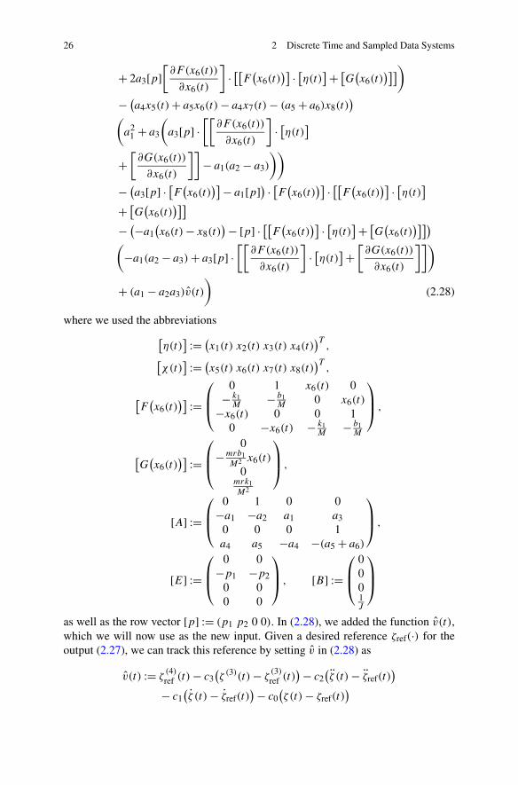
26 2 Discrete Time and Sampled Data Systems
+ 2a3[p][∂F (x6(t))
∂x6(t)
]· [[F (
x6(t))] · [η(t)
] + [G
(x6(t)
)]])
− (a4x5(t) + a5x6(t) − a4x7(t) − (a5 + a6)x8(t)
)
(a2
1 + a3
(a3[p] ·
[[∂F (x6(t))
∂x6(t)
]· [η(t)
]
+[∂G(x6(t))
∂x6(t)
]]− a1(a2 − a3)
))
− (a3[p] · [F (
x6(t))] − a1[p]) · [F (
x6(t))] · [[F (
x6(t))] · [η(t)
]
+ [G
(x6(t)
)]]
− (−a1(x6(t) − x8(t)
) − [p] · [[F (x6(t)
)] · [η(t)] + [
G(x6(t)
)]])
(−a1(a2 − a3) + a3[p] ·
[[∂F (x6(t))
∂x6(t)
]· [η(t)
] +[∂G(x6(t))
∂x6(t)
]])
+ (a1 − a2a3)v(t)
)(2.28)
where we used the abbreviations[η(t)
] := (x1(t) x2(t) x3(t) x4(t)
)T,
[χ(t)
] := (x5(t) x6(t) x7(t) x8(t)
)T,
[F
(x6(t)
)] :=⎛
⎜⎝
0 1 x6(t) 0− k1
M− b1
M0 x6(t)
−x6(t) 0 0 10 −x6(t) − k1
M− b1
M
⎞
⎟⎠ ,
[G
(x6(t)
)] :=⎛
⎜⎝
0−mrb1
M2 x6(t)
0mrk1M2
⎞
⎟⎠ ,
[A] :=⎛
⎜⎝
0 1 0 0−a1 −a2 a1 a3
0 0 0 1a4 a5 −a4 −(a5 + a6)
⎞
⎟⎠ ,
[E] :=⎛
⎜⎝
0 0−p1 −p2
0 00 0
⎞
⎟⎠ , [B] :=
⎛
⎜⎝
0001J
⎞
⎟⎠
as well as the row vector [p] := (p1 p2 0 0). In (2.28), we added the function v(t),which we will now use as the new input. Given a desired reference ζref(·) for theoutput (2.27), we can track this reference by setting v in (2.28) as
v(t) := ζ(4)ref (t) − c3
(ζ (3)(t) − ζ
(3)ref (t)
) − c2(ζ (t) − ζref(t)
)
− c1(ζ (t) − ζref(t)
) − c0(ζ(t) − ζref(t)
)

2.2 Sampled Data Systems 27
with design parameters ci ∈ R, ci ≥ 0. These parameters are degrees of freedomwithin the design of the continuous time feedback which can be used as tuningparameters, e.g., to reduce the transient time or the overshoot.
Example 2.12 Another class of systems fitting our framework, which actually goesbeyond the setting we used for introducing sampled data systems, are infinite-dimensional systems induced by partial differential equations (PDEs). In this ex-ample, we slightly change our notation in order to be consistent with the usual PDEnotation.
In the following controlled parabolic PDE (2.29) the solution y(t, x) with y :R × → R depends on time t as well as on a one-dimensional state variable x ∈ = (0,L) for a parameter L > 0. Thus, the state of the system at each time t isnow a continuous function y(t, ·) : → R and x becomes an independent variable.The control v in this example is a so-called distributed control, i.e., a measurablefunction v : R × → R. The evolution of the state is defined by the equation
yt (t, x) = θyxx(t, x) − yx(t, x) + ρ(y(t, x) − y(t, x)3) + v(t, x) (2.29)
for x ∈ and t ≥ 0 together with the initial condition y(0, x) = y0(x) and theboundary conditions y(t,0) = y(0,L) = 0.
Here yt and yx denote the partial derivatives with respect to t and x, respectivelyand yxx denotes the second partial derivative with respect to x. The parameters θ
and ρ are positive constants. Of course, in order to ensure that (2.29) is well defined,we need to interpret this equation in an appropriate weak sense and make sure thatfor the chosen class of control functions a solution to (2.29) exists in appropriatefunction spaces. For details on these issues we refer to, e.g., [10] or [18]. As wewill see later in Example 6.27, for suitable values of the parameters θ and ρ theuncontrolled equation, i.e., (2.29) with v ≡ 0, has an unstable equilibrium y∗ ≡ 0which can be stabilized by NMPC.
Using the letter z for the state of the discrete time system associated to the sam-pled data solution of (2.29), we can abstractly write this system as
z+ = f (z,u)
with z and z+ being continuous functions from to R. The function f maps y0 = z
to the solution y(T , x) of (2.29) at the sampling time T using the measurable controlfunction u = v : [0, T ] × → R. Thus, it maps continuous functions to continuousfunctions; again we omit the exact details of the respective functions spaces.
As in the ordinary differential equation case, we can restrict ourselves to the zeroorder hold situation, i.e., to control functions u(t, x) which are constant in t ∈ [0, T ].The corresponding control functions v generated via (2.11) are again constant in t oneach sampling interval [tn, tn+1). Note, however, that in our distributed control con-text both u and v are still arbitrary measurable—i.e., in particular non-constant—functions in x.
For sampled data systems, the nominal closed-loop system (2.5) corresponds tothe closed-loop sampled data system
x(t) = fc
(x(t),μ
(x(tn)
)(t − tn)
), t ∈ [tn, tn+1), n = 0,1,2, . . . (2.30)

28 2 Discrete Time and Sampled Data Systems
whose solution with initial value x0 ∈ X we denote by ϕ(t, t0, x0,μ). Note thatthe argument “(t − tn)” of μ(x(tn)) can be dropped in case of sampling with zeroorder hold when—as usual—we interpret the control value μ(x(tn)) ∈ U = R
m as aconstant control function.
2.3 Stability of Discrete Time Systems
In the introduction, we already specified the main goal of model predictive control,namely to control the state x(n) of the system toward a reference trajectory xref(n)
and then keep it close to this reference. In this section we formalize what we mean by“toward” and “close to” using concepts from stability theory of nonlinear systems.
We first consider the case where xref is constant, i.e., where xref ≡ x∗ holds forsome x∗ ∈ X. We assume that the states x(n) are generated by a difference equationof the form
x+ = g(x) (2.31)
for a not necessarily continuous map g : X → X via the usual iteration x(n + 1) =g(x(n)). As before, we write x(n, x0) for the trajectory satisfying the initial condi-tion x(0, x0) = x0 ∈ X. Allowing g to be discontinuous is important for our NMPCapplication, because g will later represent the nominal closed-loop system (2.5) con-trolled by the NMPC-feedback law μ, i.e., g(x) = f (x,μ(x)). Since μ is obtainedas an outcome of an optimization algorithm, in general we cannot expect μ to becontinuous and thus g will in general be discontinuous, too.
Nonlinear stability properties can be expressed conveniently via so-called com-parison functions, which were first introduced by Hahn in 1967 [5] and popularizedin nonlinear control theory during the 1990s by Sontag, particularly in the contextof input-to-state stability [14]. Although we mainly deal with discrete time systems,we stick to the usual continuous time definition of these functions using the notationR
+0 = [0,∞).
Definition 2.13 We define the following classes of comparison functions:
K := {α : R
+0 → R
+0
∣∣ α is continuous & strictly increasing with α(0) = 0},
K∞ := {α : R
+0 → R
+0
∣∣ α ∈ K, α is unbounded},
L :={δ : R
+0 → R
+0
∣∣∣ δ is continuous & strictly decreasing with limt→∞ δ(t) = 0
},
K L := {β : R
+0 × R
+0 → R
+0
∣∣ β is continuous, β(·, t) ∈ K, β(r, ·) ∈ L}.
The graph of a typical function β ∈ K L is shown in Fig. 2.6.Using this function, we can now introduce the concept of asymptotic stability.
Here, for arbitrary x1, x2 ∈ X we denote the distance from x1 to x2 by
|x1|x2 := dX(x1, x2).

2.3 Stability of Discrete Time Systems 29
Fig. 2.6 Illustration of a typical class K L function
Furthermore, we use the ball
Bη(x∗) := {x ∈ X
∣∣ |x|x∗ < η}
and we say that a set Y ⊆ X is forward invariant for (2.31) if g(x) ∈ Y holds for allx ∈ Y .
Definition 2.14 Let x∗ ∈ X be an equilibrium for (2.31), i.e., g(x∗) = x∗. Then wesay that x∗ is locally asymptotically stable if there exist η > 0 and a function β ∈ K Lsuch that the inequality
∣∣x(n, x0)∣∣x∗ ≤ β
(|x0|x∗ , n)
(2.32)
holds for all x0 ∈ Bη(x∗) and all n ∈ N0.We say that x∗ is asymptotically stable on a forward invariant set Y with x∗ ∈ Y
if there exists β ∈ K L such that (2.32) holds for all x0 ∈ Y and all n ∈ N0 and wesay that x∗ is globally asymptotically stable if x∗ is asymptotically stable on Y = X.
If one of these properties holds then β is called attraction rate.
Note that asymptotic stability on a forward invariant set Y implies local asymp-totic stability if Y contains a ball Bη(x∗). However, we do not necessarily requirethis property.
Asymptotic stability thus defined consists of two main ingredients.
(i) The smaller the initial distance from x0 to x∗ is, the smaller the distance fromx(n) to x∗ becomes for all future n, or formally: for each ε > 0 there exists δ > 0such that |x(n, x0)|x∗ ≤ ε holds for all n ∈ N0 and all x0 ∈ Y (or x0 ∈ Bη(x∗))with |x0|x∗ ≤ δ.
This fact is easily seen by choosing δ so small that β(δ,0) ≤ ε holds, whichis possible since β(·,0) ∈ K. Since β is decreasing in its second argument, for|x0|x∗ ≤ δ from (2.32) we obtain
∣∣x(n, x0)∣∣x∗ ≤ β
(|x0|x∗, n) ≤ β
(|x0|x∗,0) ≤ β(δ,0) ≤ ε.

30 2 Discrete Time and Sampled Data Systems
Fig. 2.7 Sketch ofasymptotic stability (left) asopposed to practicalasymptotic stability (right)
(ii) As the system evolves, the distance from x(n, x0) to x∗ becomes arbitrarilysmall, or formally: for each ε > 0 and each R > 0 there exists N > 0 suchthat |x(n, x0)|x∗ ≤ ε holds for all n ≥ N and all x0 ∈ Y (or x0 ∈ Bη(x∗)) with|x0|x∗ ≤ R. This property easily follows from (2.32) by choosing N > 0 withβ(R,N) ≤ ε and exploiting the monotonicity properties of β .
These two properties are known as (i) stability (in the sense of Lyapunov) and (ii)attraction. In the literature, asymptotic stability is often defined via these two prop-erties. In fact, for continuous time (and continuous) systems (i) and (ii) are known tobe equivalent to the continuous time counterpart of Definition 2.14, cf. [8, Sect. 3].We conjecture that the arguments in this reference can be modified in order to provethat equivalence also holds for our discontinuous discrete time setting.
Asymptotic stability includes the desired properties of the NMPC closed loopdescribed earlier: whenever we are already close to the reference equilibrium wewant to stay close; otherwise we want to move toward the equilibrium.
Asymptotic stability also includes that eventually the distance of the closed-loopsolution to the equilibrium x∗ becomes arbitrarily small. Occasionally, this maybe too demanding. In the following chapters, this is for instance the case if thesystem is subject to perturbations or modeling errors, cf. Sects. 8.5–8.9 or if inNMPC without stabilizing terminal constraints the system cannot be controlled tox∗ sufficiently fast, cf. Sect. 6.7. In this case, one can relax the asymptotic stabilitydefinition to practical asymptotic stability as follows. Here we only consider thecase of asymptotic stability on a forward invariant set Y .
Definition 2.15 Let Y be a forward invariant set and let P ⊂ Y be a subset of Y .Then we say that a point x∗ ∈ P is P -practically asymptotically stable on Y if thereexists β ∈ K L such that (2.32) holds for all x0 ∈ Y and all n ∈ N0 with x(n, x0) /∈ P .
Figure 2.7 illustrates practical asymptotic stability (on the right) as opposed to“usual” asymptotic stability (on the left).
This definition is typically used with P contained in a small ball around theequilibrium, i.e., P ⊆ Bδ(x∗) for some small δ > 0. In this case one obtains theestimate
∣∣x(n, x0)∣∣x∗ ≤ max
{β(|x0|x∗ , n
), δ
}(2.33)
for all x0 ∈ Y and all n ∈ N0, i.e., the system behaves like an asymptotically stablesystem until it reaches the ball Bδ(x∗). Note that x∗ does not need to be an equilib-rium in Definition 2.15.

2.3 Stability of Discrete Time Systems 31
For general non-constant reference functions xref : N0 → X we can easily extendDefinition 2.14 if we take into account that the objects under consideration becometime varying in two ways: (i) the distance under consideration varies with n and(ii) the system (2.31) under consideration varies with n. While (i) is immediate, (ii)follows from the fact that with time varying reference also the feedback law μ istime varying, i.e., we obtain a feedback law of the type μ(n,x(n)). Consequently,we now need to consider systems
x+ = g(n, x) (2.34)
with g of the form g(n, x) = f (x,μ(n, x)). Furthermore, we now have to take theinitial time n0 into account: while the solutions of (2.31) look the same for all initialtimes n0 (which is why we only considered n0 = 0) now we need to keep track ofthis value. To this end, by x(n,n0, x0) we denote the solution of (2.34) with initialcondition x(n0, n0, x0) = x0 at time n0. The appropriate modification of Defini-tion 2.14 then looks as follows. Here we say that a time-dependent family of setsY(n) ⊆ X, n ∈ N0 is forward invariant if g(n, x) ∈ Y(n + 1) holds for all n ∈ N0and all x ∈ Y(n).
Definition 2.16 Let xref : N0 → X be a trajectory for (2.31), i.e., xref(n + 1) =g(xref(n)) for all n ∈ N0. Then we say that xref is locally uniformly asymptoticallystable if there exists η > 0 and a function β ∈ K L such that the inequality
∣∣x(n,n0, x0)∣∣xref(n)
≤ β(|x0|xref(n0)
, n − n0)
(2.35)
holds for all x0 ∈ Bη(xref(n0)) and all n0, n ∈ N0 with n ≥ n0.
We say that x∗ is uniformly asymptotically stable on a forward invariant familyof sets Y(n) with xref(n) ∈ Y(n) if there exists β ∈ K L such that (2.35) holds for alln0, n ∈ N0 with n ≥ n0 and all x0 ∈ Y(n0) and we say that x∗ is globally uniformlyasymptotically stable if x∗ is asymptotically stable on Y(n) = X for all n0 ∈ N0.
If one of these properties hold then β is called (uniform) attraction rate.
The term “uniform” describes the fact that the bound β(|x0|xref(n0), n − n0) only
depends on the elapsed time n − n0 but not on the initial time n0. If this were thecase, i.e., if we needed different β for different initial times n0, then we would callthe asymptotic stability “nonuniform”. For a comprehensive discussion of nonuni-form stability notions and their representation via time-dependent K L functions werefer to [3].
As in the time-invariant case, asymptotic stability on a forward invariant fam-ily of sets Y(n) implies local asymptotic stability if each Y(n) contains a ball
Bη(xref(n)). Again, we do not necessarily require this property.
The time varying counterpart of P -practical asymptotic stability is defined asfollows.
Definition 2.17 Let Y(n) be a forward invariant family of sets and let P(n) ⊂ Y(n)
be subsets of Y(n). Then we say that a reference trajectory xref with xref(n) ∈ P(n)
is P -practically uniformly asymptotically stable on Y(n) if there exists β ∈ K L such

32 2 Discrete Time and Sampled Data Systems
that (2.35) holds for all x0 ∈ Y(n0) and all n0, n ∈ N0 with n ≥ n0 and x(n,n0, x0) /∈P(n).
Analogous to the time-invariant case, this definition is typically used withP(n) ⊆ Bδ(x
ref(n)) for some small value δ > 0, which then yields∣∣x(n,n0, x0)
∣∣xref(n)
≤ max{β(|x0|xref(n0)
, n − n0), δ
}. (2.36)
In order to verify that our NMPC controller achieves asymptotic stability wewill utilize the concept of Lyapunov functions. For constant reference xref ≡ x∗ ∈ X
these functions are defined as follows.
Definition 2.18 Consider a system (2.31), a point x∗ ∈ X and let S ⊆ X be a subsetof the state space. A function V : S → R
+0 is called a Lyapunov function on S if the
following conditions are satisfied:
(i) There exist functions α1, α2 ∈ K∞ such that
α1(|x|x∗
) ≤ V (x) ≤ α2(|x|x∗
)(2.37)
holds for all x ∈ S.(ii) There exists a function αV ∈ K such that
V(g(x)
) ≤ V (x) − αV
(|x|x∗)
(2.38)
holds for all x ∈ S with g(x) ∈ S.
The following theorem shows that the existence of a Lyapunov function ensuresasymptotic stability.
Theorem 2.19 Let x∗ be an equilibrium of (2.31) and assume there exists a Lya-punov function V on S. If S contains a ball Bν(x∗) with g(x) ∈ S for all x ∈ Bν(x∗)then x∗ is locally asymptotically stable with η = α−1
2 ◦ α1(ν). If S = Y holds forsome forward invariant set Y ⊆ X containing x∗ then x∗ is asymptotically stable onY . If S = X holds then x∗ is globally asymptotically stable.
Proof The idea of the proof lies in showing that by (2.38) the function V (x(n, x0))
is strictly decreasing in n and converges to 0. Then by (2.37) we can conclude thatx(n, x0) converges to x∗. The function β from Definition 2.14 will be constructedfrom α1, α2 and αV . In order to simplify the notation, throughout the proof we write|x| instead of |x|x∗ .
First, if S is not forward invariant, define the value γ := α1(ν) and the set S :={x ∈ X |V (x) < γ }. Then from (2.37) we get
x ∈ S ⇒ α1(|x|) ≤ V (x) < γ ⇒ |x| < α−1
1 (γ ) = ν ⇒ x ∈ Bν(x∗),
observing that each α ∈ K∞ is invertible with α−1 ∈ K∞.Hence, for each x ∈ S Inequality (2.38) applies and consequently V (g(x)) ≤
V (x) < γ implying g(x) ∈ S. If S = Y for some forward invariant set Y ⊆ X we
2.3 Stability of Discrete Time Systems 33
define S := S. With these definitions, in both cases the set S becomes forward in-variant.
Now we define α′V := αV ◦ α−1
2 . Note that concatenations of K-functions areagain in K, hence α′
V ∈ K. Since |x| ≥ α−12 (V (x)), using monotonicity of αV this
definition implies
αV
(|x|) ≥ αV ◦ α−12
(V (x)
) = α′V
(V (x)
).
Hence, along a trajectory x(n, x0) with x0 ∈ S, from (2.38) we get the inequality
V(x(n + 1, x0)
) ≤ V(x(n, x0)
) − αV
(∣∣x(n, x0)∣∣)
≤ V(x(n, x0)
) − α′V
(V
(x(n, x0)
)). (2.39)
For the construction of β we need the last expression in (2.39) to be strictlyincreasing in V (x(n, x0)). To this end we define
αV (r) := mins∈[0,r]
{α′
V (s) + (r − s)/2}.
Straightforward computations show that this function satisfies r2 − αV (r2) > r1 −αV (r1) ≥ 0 for all r2 > r1 ≥ 0 and min{α′
V (r/2), r/4} ≤ αV (r) ≤ α′V (r) for all
r ≥ 0. In particular, (2.39) remains valid and we get the desired monotonicity whenα′
V is replaced by αV .We inductively define a function β1 : R
+0 × N0 → R
+0 via
β1(r,0) := r, β1(r, n + 1) = β1(r, n) − αV
(β1(r, n)
). (2.40)
By induction over n using the properties of αV (r) and Inequality (2.39) one easilyverifies the following inequalities:
β1(r2, n) > β1(r1, n) ≥ 0 for all r2 > r1 ≥ 0 and all n ∈ N0, (2.41)
β1(r, n1) > β1(r, n2) > 0 for all n2 > n1 ≥ 0 and all r > 0, (2.42)
V(x(n, x0)
) ≤ β1(V (x0), n
)for all n ∈ N0 and all x0 ∈ S. (2.43)
From (2.42) it follows that β1(r, n) is monotone decreasing in n and by (2.41)it is bounded from below by 0. Hence, for each r ≥ 0 the limit β∞
1 (r) =limn→∞ β1(r, n) exists. We claim that β∞
1 (r) = 0 holds for all r . Indeed, con-vergence implies β1(r, n) − β1(r, n + 1) → 0 as n → ∞, which together with(2.40) yields αV (β1(r, n)) → 0. On the other hand, since αV is continuous, weget αV (β1(r, n)) → αV (β∞
1 (r)). This implies
αV
(β∞
1 (r)) = 0,
which, because of αV (r) ≥ min{α′V (r/2), r/4} and α′
V ∈ K, is only possible ifβ∞
1 (r) = 0.Consequently, β1(r, n) has all properties of a K L function except that it is only
defined for n ∈ N0. Defining the linear interpolation
β2(r, t) := (n + 1 − t)β1(r, n) + (t − n)β1(r, n + 1)

34 2 Discrete Time and Sampled Data Systems
for t ∈ [n,n + 1) and n ∈ N0, we obtain a function β2 ∈ K L which coincides withβ1 for t = n ∈ N0. Finally, setting
β(r, t) := α−11 ◦ β2
(α2(r), t
)
we can use (2.43) in order to obtain∣∣x(n, x0)
∣∣ ≤ α−11
(V
(x(n, x0)
)) ≤ α−11 ◦ β1
(V (x0), n
)
= α−11 ◦ β2
(V (x0), n
) ≤ α−11 ◦ β2
(α2
(|x0|), n
) = β(|x0|, n
),
for all x0 ∈ S and all n ∈ N0. This is the desired Inequality (2.32). If S = S = Y
this shows the claimed asymptotic stability on Y and global asymptotic stabilityif Y = X. If S = S, then in order to satisfy the local version of Definition 2.14 itremains to show that x ∈ Bη(x∗) implies x ∈ S. Since by definition of η and γ wehave η = α−1
2 (γ ), we get
x ∈ Bη(x∗) ⇒ |x| < η = α−12 (γ ) ⇒ V (x) ≤ α2
(|x|) < γ ⇒ x ∈ S.
This finishes the proof. �
Likewise, P -practical asymptotic stability can be ensured by a suitable Lyapunovfunction condition provided the set P is forward invariant.
Theorem 2.20 Consider forward invariant sets Y and P ⊂ Y and a point x∗ ∈ P .If there exists a Lyapunov function V on S = Y \ P then x∗ is P -practically asymp-totically stable on Y .
Proof The same construction of β as in the proof of Theorem 2.19 yields∣∣x(n, x0)
∣∣x∗ ≤ β
(|x|x∗, n)
(2.32)
for all n = 0, . . . , n∗ − 1, where n∗ ∈ N0 is minimal with x(n∗, x0) ∈ P . This fol-lows with the same arguments as in the proof of Theorem 2.19 by restricting thetimes considered in (2.39) and (2.43) to n = 0, . . . , n∗ − 2 and n = 0, . . . , n∗ − 1,respectively.
Since forward invariance of P ensures x(n, x0) ∈ P for all n ≥ n∗, the times n
for which x(n, x0) /∈ P holds are exactly n = 0, . . . , n∗ − 1. Since these are exactlythe times at which (2.32) is required, this yields the desired P -practical asymptoticstability. �
In case of a time varying reference xref we need to use the time varying asymp-totic stability from Definition 2.16. The corresponding Lyapunov function conceptis as follows.
Definition 2.21 Consider a system (2.34), reference points xref(n), subsets of thestate space S(n) ⊆ X and define S := {(n, x) |n ∈ N0, x ∈ S(n)}. A function V :
S → R+0 is called a uniform time varying Lyapunov function on S(n) if the following
conditions are satisfied:

2.4 Stability of Sampled Data Systems 35
(i) There exist functions α1, α2 ∈ K∞ such that
α1(|x|xref(n)
) ≤ V (n, x) ≤ α2(|x|xref(n)
)(2.44)
holds for all n ∈ N0 and all x ∈ S(n).(ii) There exists a function αV ∈ K such that
V(n + 1, g(n, x)
) ≤ V (n, x) − αV
(|x|xref(n)
)(2.45)
holds for all n ∈ N0 and all x ∈ S(n) with g(n, x) ∈ S(n + 1).
Theorem 2.22 Let xref be a trajectory of (2.34) and assume there exists a uniformtime varying Lyapunov function V on S(n). If each S(n) contains a ball Bν(x
ref(n))
with g(n, x) ∈ S(n + 1) for all x ∈ Bν(xref(n)) then xref is locally asymptotically
stable with η = α−12 ◦ α1(ν). If the family of sets S(n) is forward invariant in the
sense stated before Definition 2.16, then xref is asymptotically stable on S(n). IfS(n) = X holds for all n ∈ N0 then xref is globally asymptotically stable.
Proof The proof is analogous to the proof of Theorem 2.19 with the obvious modi-fications to take n ∈ N0 into account. �
Indeed, the necessary modification in the proof are straightforward because thetime varying Lyapunov function is uniform, i.e., α1, α2 and αV do not depend on n.For the more involved nonuniform case we again refer to [3].
The P -practical version of this statement is provided by the following theorem inwhich we assume forward invariance of the sets P(n). Observe that here xref doesnot need to be a trajectory of the system (2.34).
Theorem 2.23 Consider forward invariant families of sets Y(n) and P(n) ⊂ Y(n),n ∈ N0, and reference points xref(n) ∈ P(n). If there exists a uniform time varyingLyapunov function V on S(n) = Y(n) \ P(n) then xref is P -practically asymptoti-cally stable on Y(n).
Proof The proof is analogous to the proof of Theorem 2.20 with the obvious modi-fications. �
2.4 Stability of Sampled Data Systems
We now investigate the special case in which (2.31) represents the nominal closed-loop system (2.5) with f obtained from a sampled data system via (2.8). In this case,the solutions x(n, x0) of (2.31) and the solutions ϕ(tn, t0, x0,μ) of the sampled dataclosed-loop system (2.30) satisfy the identity
x(n, x0) = ϕ(tn, t0, x0,μ) (2.46)

36 2 Discrete Time and Sampled Data Systems
for all n ∈ N0. This implies that the stability criterion from Definition 2.14 (and anal-ogous for the other stability definitions) only yields inequalities for the continuousstate of the system at the sampling times tn, i.e.,
∣∣ϕ(tn, t0, x0,μ)∣∣x∗ ≤ β
(|x0|x∗, n)
for all n = 0,1,2, . . . (2.47)
for a suitable β ∈ K L. However, for a continuous time system it is in general de-sirable to ensure the existence of β ∈ K L such that the continuous time asymptoticstability property
∣∣ϕ(t, t0, x0,μ)
∣∣x∗ ≤ β
(|x0|x∗, t)
for all t ≥ 0 (2.48)
holds.In the remainder of this chapter we will show that under a reasonable additional
assumption (2.47) implies the existence of β ∈ K L such that (2.48) holds. For sim-plicity, we restrict ourselves to local asymptotic stability and to the case of time-invariant reference xref ≡ x∗. The arguments can be modified to cover the othercases, as well.
The necessary additional condition is the following boundedness assumption onthe solutions in between two sampling instants.
Definition 2.24 Consider a sampled data closed-loop system (2.30) with samplingperiod T > 0. If there exists a function γ ∈ K and a constant η > 0 such that for allx ∈ X with |x|x∗ ≤ η, the solutions of (2.30) exist on [0, T ] and satisfy
∣∣ϕ(t,0, x,μ)∣∣x∗ ≤ γ
(|x|x∗)
for all t ∈ [0, T ] then the solutions of (2.30) are called uniformly bounded over T .
Effectively, this condition demands that in between two sampling times tn andtn+1 the continuous time solution does not deviate too much from the solution atthe sampling time tn. Sufficient conditions for this property formulated directly interms of the vector field fc in (2.30) can be found in [11, Lemma 3]. A sufficientcondition in our NMPC setting is discussed in Remark 4.13.
For the subsequent analysis we introduce the following class of K L functions,which will allow us to deal with the inter sampling behavior of the continuous timesolution.
Definition 2.25 A function β ∈ K L is called uniformly incrementally bounded ifthere exists P > 0 such that β(r, k) ≤ Pβ(r, k + 1) holds for all r ≥ 0 and all k ∈ N.
Uniformly incrementally bounded K L functions exhibit a nice bounding prop-erty compared to standard K L functions which we will use the proof of Theo-rem 2.27. Before, we show that any K L function β—like the one in (2.47)—canbe bounded from above by a uniformly incrementally bounded K L function.

2.4 Stability of Sampled Data Systems 37
Lemma 2.26 For any β ∈ K L the function
β(r, t) := maxτ∈[0,t]
2−τ β(r, t − τ)
is a uniformly incrementally bounded K L function with β(r, t) ≤ β(r, t) for all r ≥ 0and all t ≥ 0 and P = 2.
Proof The inequality β ≤ β follows immediately from the definition. Uniform in-cremental boundedness with P = 2 follows from the inequality
β(r, t) = maxτ∈[0,t] 2−τ β(r, t − τ) = max
τ∈[1,t+1] 21−τ β(r, t − τ + 1)
= 2 maxτ∈[1,t+1] 2−τβ(r, t − τ + 1) ≤ 2 max
τ∈[0,t+1] 2−τ β(r, t − τ + 1)
= 2β(r, t + 1).
It remains to show that β ∈ K L.Since β ∈ K L it follows that β is continuous and β(0, t) = 0 for any t ≥ 0. For
any r2 > r1 ≥ 0, β ∈ K L implies 2−τ β(r2, t − τ) > 2−τ β(r1, t − τ). This showsthat β(r2, t) > β(r1, t) and hence β(·, t) ∈ K.
Next we show that for any fixed r > 0 the function t �→ β(r, t) is strictly decreas-ing to 0. To this end, in the following we use that for all t ≥ s ≥ q ≥ 0 and all r ≥ 0the inequality
maxτ∈[q,s] 2−τ β(r, t − τ) ≤ 2−qβ(r, t − s)
holds. In order to show the strict decrease property for r > 0, let t2 > t1 ≥ 0. Defin-ing d := t2 − t1 we obtain
β(r, t2) = maxτ∈[0,t2]
2−τ β(r, t2 − τ)
= max{
maxτ∈[0,d/2]
2−τ β(r, t2 − τ), maxτ∈[d/2,d]
2−τ β(r, t2 − τ),
maxτ∈[d,t2]
2−τβ(r, t2 − τ)}
≤ max{β(r, t2 − d/2),2−d/2β(r, t2 − d), max
τ∈[0,t1]2−τ−dβ(r, t1 − τ)
}
= max{β(r, t1 + d/2),2−d/2β(r, t1),2−d β(r, t1)
}.
Now the strict monotonicity β(r, t2) < β(r, t1) follows since β(r, t1 + d/2) <
β(r, t1) ≤ β(r, t1), 2−d/2β(r, t1) < β(r, t1) ≤ β(r, t1) and 2−d β(r, t1) < β(r, t1).Finally, we prove limt→∞ β(r, t) = 0 for any r > 0. Since
β(r, t) ≤ max{
maxτ∈[0,t/2] 2−τ β(r, t − τ), max
τ∈[t/2,t] 2−τ β(r, t − τ)}
≤ max{β(r, t/2),2−t/2β(r,0)
} → 0 as t → ∞the assertion follows. �
Now, we are ready to prove the final stability result.

38 2 Discrete Time and Sampled Data Systems
Theorem 2.27 Consider the sampled data closed-loop system (2.30) with samplingperiod T > 0 and the corresponding discrete time closed-loop system (2.5) with f
from (2.8). Then (2.30) is locally asymptotically stable, i.e., there exists η > 0 andβ ∈ K L such that (2.48) holds for all x ∈ Bη(x∗), if and only if (2.5) is locallyasymptotically stable and the solutions of (2.30) are uniformly bounded over T .
Proof If (2.30) is locally asymptotically stable with some β ∈ K L, then by (2.46)it immediately follows that the discrete time system (2.5) is asymptotically stablewith β(r, k) = β(r, kT ) and that the solutions of (2.30) are uniformly bounded withγ (r) = β(r,0).
Conversely, assume that (2.5) is locally asymptotically stable and that the solu-tions of (2.30) are uniformly bounded over T . Denote the values η > 0 from Defini-tion 2.14 and Definition 2.24 by ηs and ηb , respectively. These two properties implythat there exist β ∈ K L and γ ∈ K∞ such that
|x|x∗ ≤ ηs �⇒ ∣∣ϕ(kT ,0, x,μ)∣∣x∗ ≤ β
(|x|x∗, k)
for all k ≥ 0, (2.49)
|x|x∗ ≤ ηb �⇒ ∣∣ϕ(t,0, x,μ)∣∣x∗ ≤ γ
(|x|x∗)
for all t ∈ [0, T ]. (2.50)
In order to show the assertion we have to construct η > 0 and β ∈ K L with
|x|x∗ ≤ η �⇒ ∣∣ϕ(t,0, x,μ)
∣∣x∗ ≤ β
(|x|x∗, t)
for all t ≥ 0. (2.51)
Define γ0(r) := β(r,0) and let η = min{ηs, γ −10 (ηb)}. This definition implies
β(η,0) ≤ ηb and η ≤ ηs . In what follows we consider arbitrary x ∈ X with |x|x∗ ≤η. For these x, (2.49) and η ≤ ηs yield
∣∣ϕ(kT ,0, x,μ)∣∣x∗ ≤ β
(‖x‖x∗, k) ≤ β(η,0) ≤ ηb for all k ≥ 0. (2.52)
For any k ≥ 0 and t ∈ [kT , (k + 1)T ] the definition of (2.30) implies
ϕ(t,0, x,μ) = ϕ(t − kT ,0, ϕ(kT ,0, x,μ),μ
).
Since (2.52) implies |ϕ(kT ,0, x,μ)|x∗ ≤ ηb for all k ≥ 0, (2.50) holds for x =ϕ(kT ,0, x,μ) and from (2.50) and (2.52) we obtain
∣∣ϕ(t,0, x,μ)∣∣x∗ ≤ γ
(∥∥ϕ(kT ,0, x,μ)∥∥) ≤ γ
(β(‖x‖x∗, k
))(2.53)
for all t ∈ [kT , (k + 1)T ] and all k ≥ 0.Now we define β(r, t) := γ (β(r, t)). Clearly, β ∈ K L and by Lemma 2.26 we
can assume without loss of generality that β is uniformly incrementally bounded;otherwise we replace it by β from this lemma.
Hence, for k ∈ N0 and s ∈ [0,1] we obtain
β(r, k) ≤ P β(r, k + 1) ≤ P β(r, k + s). (2.54)
Now pick an arbitrary t ≥ 0 and let k ∈ N0 be maximal with k ≤ t/T . Then (2.53)and (2.54) with s = t/T − k ∈ [0,1] imply
∣∣ϕ(t,0, x,μ)∣∣x∗ ≤ β
(‖x‖x∗, k) ≤ P β
(|x|x∗, k + (t/T − k)) = P β
(|x|x∗, t/T).
This shows the assertion with β(r, t) = P β(r, t/T ). �

2.5 Notes and Extensions 39
Concluding, if we can compute an asymptotically stabilizing feedback law forthe discrete time system induced by the sampled data system, then the resultingcontinuous time sampled data closed loop is also asymptotically stable provided itssolutions are uniformly bounded over T .
2.5 Notes and Extensions
The general setting presented in Sect. 2.1 is more or less standard in discrete timecontrol theory, except maybe for the rather general choice of the state space X andthe control value space U which allows us to cover infinite-dimensional systems asillustrated in Example 2.12 and sampled data systems without the zero order holdassumption as discussed after Theorem 2.7.
This definition of sampled data systems is not so frequently found in the litera-ture, where often only the special case of zero order hold is discussed. While zeroorder hold is usually the method of choice in practical applications and is also usedin the numerical examples later in this book, for theoretical investigations the moregeneral approach given in Sect. 2.2 is appealing, too.
The discrete time stability theory presented in Sect. 2.3 has a continuous timecounterpart, which is actually more frequently found in the literature. Introductorytextbooks on this subject in a control theoretic setting are, e.g., the books by Khalil[7] and Sontag [15]. The proofs in this section are not directly taken from the liter-ature, but they are based on standard arguments, which appear in many books andpapers on the subject. Formulating asymptotic stability via K L-function goes backto Hahn [5] and became popular in nonlinear control theory during the 1990s via theinput-to-state stability (ISS) property introduced by Sontag in [14]. A good surveyon this theory can be found in Sontag [16].
While here we only stated direct Lyapunov function theorems which state that theexistence of a Lyapunov function ensures asymptotic stability, there is a rather com-plete converse theory, which shows that asymptotic stability implies the existenceof Lyapunov functions. A collection of such results—again in a control theoreticsetting—can be found in the PhD thesis of Kellett [6].
The final Sect. 2.4 on asymptotic stability of sampled data systems is based on thePaper [11] by Nešic, Teel and Sontag, in which this topic is treated in a more generalsetting. In particular, this paper also covers ISS results for perturbed systems.
2.6 Problems
1. Show that there exists no differential equation x(t) = fc(x(t)) (i.e., without con-trol input) satisfying Assumption 2.4 and fc(0) = 0 such that the difference equa-tion x+ = f (x) with
f (x) ={
x2 , x ≥ 0,
−x, x < 0
is the corresponding sampled data system.

40 2 Discrete Time and Sampled Data Systems
2. (a) Show that xref(n) = ∑nk=0
12n−k sin(k) is a solution of the difference equation
x(n + 1) = 1
2x(n) + sin(n).
(b) Prove that xref from (a) is uniformly asymptotically stable and derive a com-parison function β ∈ K L such that (2.35) holds. Here it is sufficient to derivea formula for β(r, n) for n ∈ N0.
(c) Show that xref(n) = ∑nk=0
k+1n+1 sin(k) is a solution of the difference equation
x(n + 1) = n + 1
n + 2x(n) + sin(n).
(d) Can you also prove uniform asymptotic stability for xref from (c)?Hint for (b) and (d): One way to proceed is to derive a difference equation
for z(n) = x(n,n0, x0) − xref(n) and look at the equilibrium x∗ = 0 for this newequation.
3. Consider the two-dimensional difference equation
x+ = (1 − ‖x‖)
(0 1
−1 0
)x
with x = (x1, x2)� ∈ R
2.(a) Prove that V (x) = x2
1 +x22 is a Lyapunov function for the equilibrium x∗ = 0
on S = {x ∈ R2 | ‖x‖ ≤ 1}.
(b) Is V also a Lyapunov function on S = R2?
(c) Solve (a) and (b) for the difference equation
x+ = 1
1 + ‖x‖(
0 1−1 0
)x.
4. Consider a globally asymptotically stable difference equation (2.31) with equi-librium x∗ ∈ X and a Lyapunov function V on S = X with α1(r) = 2r2,α2(r) = 3r2 and αV (r) = r2.
Compute the rate of attraction β ∈ K L such that (2.32) holds. Here it is suffi-cient to derive a formula for β(r, n) for n ∈ N0.
Hint: Follow the construction of β from the proof of Theorem 2.19. Why canyou use αV = α′
V for this problem?5. Consider a difference equation (2.31) with equilibrium x∗ ∈ X and a function
V : X → R+0 which satisfies (2.37) but only
V(g(x)
) ≤ V (x)
instead of (2.38).(a) Prove that there exists αL ∈ K∞ such that the solutions of (2.1) satisfy the
inequality∣∣x(n, x0)
∣∣x∗ ≤ αL
(|x0|).
(b) Conclude from (a) that the system is stable in the sense of Lyapunov, cf. thediscussion after Definition 2.14.

References 41
References
1. Freeman, R.A., Kokotovic, P.V.: Robust Nonlinear Control Design. Systems & Control: Foun-dations & Applications. Birkhäuser, Boston (1996)
2. Giselsson, P., Åkesson, J., Robertsson, A.: Optimization of a pendulum system using optimicaand modelica. In: 7th International Modelica Conference 2009. Modelica Association (2009)
3. Grüne, L., Kloeden, P.E., Siegmund, S., Wirth, F.R.: Lyapunov’s second method for nonau-tonomous differential equations. Discrete Contin. Dyn. Syst. 18(2–3), 375–403 (2007)
4. Grüne, L., Nešic, D., Pannek, J., Worthmann, K.: Redesign techniques for nonlinear sampled-data systems. Automatisierungstechnik 56(1), 38–47 (2008)
5. Hahn, W.: Stability of Motion. Springer, Berlin (1967)6. Kellett, C.M.: Advances in converse and control Lyapunov functions. PhD thesis, University
of California, Santa Barbara (2000)7. Khalil, H.K.: Nonlinear Systems, 3rd edn. Prentice Hall, Upper Saddle River (2002)8. Lin, Y., Sontag, E.D., Wang, Y.: A smooth converse Lyapunov theorem for robust stability.
SIAM J. Control Optim. 34(1), 124–160 (1996)9. Magni, L., Scattolini, R., Aström, K.J.: Global stabilization of the inverted pendulum using
model predictive control. In: Proceedings of the 15th IFAC World Congress (2002)10. Neittaanmäki, P., Tiba, D.: Optimal Control of Nonlinear Parabolic Systems. Theory, Al-
gorithms, and Applications. Monographs and Textbooks in Pure and Applied Mathematics,vol. 179. Dekker, New York (1994)
11. Nešic, D., Teel, A.R., Sontag, E.D.: Formulas relating K L stability estimates of discrete-timeand sampled-data nonlinear systems. Systems Control Lett. 38(1), 49–60 (1999)
12. Nešic, D., Grüne, L.: A receding horizon control approach to sampled-data implementation ofcontinuous-time controllers. Systems Control Lett. 55, 660–672 (2006)
13. Pannek, J.: Receding horizon control: a suboptimality-based approach. PhD thesis, Universityof Bayreuth, Germany (2009)
14. Sontag, E.D.: Smooth stabilization implies coprime factorization. IEEE Trans. Automat. Con-trol 34(4), 435–443 (1989)
15. Sontag, E.D.: Mathematical Control Theory, 2nd edn. Texts in Applied Mathematics, vol. 6.Springer, New York (1998)
16. Sontag, E.D.: Input to state stability: basic concepts and results. In: Nonlinear and OptimalControl Theory. Lecture Notes in Mathematics, vol. 1932, pp. 163–220. Springer, Berlin(2008)
17. Stewart, D.E.: Rigid-body dynamics with friction and impact. SIAM Rev. 42(1), 3–39 (2000)18. Tröltzsch, F.: Optimal Control of Partial Differential Equations. Graduate Studies in Mathe-
matics, vol. 112. American Mathematical Society, Providence (2010). Theory, methods andapplications. Translated from the 2005 German original by Jürgen Sprekels


Chapter 3Nonlinear Model Predictive Control
In this chapter, we introduce the nonlinear model predictive control algorithm in arigorous way. We start by defining a basic NMPC algorithm for constant referenceand continue by formalizing state and control constraints. Viability (or weak forwardinvariance) of the set of state constraints is introduced and the consequences for theadmissibility of the NMPC feedback law are discussed. After having introducedNMPC in a special setting, we describe various extensions of the basic algorithm,considering time varying reference solutions, terminal constraints and costs and ad-ditional weights. Finally, we investigate the optimal control problem correspondingto this generalized setting and prove several properties, most notably the dynamicprogramming principle.
3.1 The Basic NMPC Algorithm
As already outlined in the introductory Chap. 1, the idea of the NMPC scheme is asfollows: at each sampling instant n we optimize the predicted future behavior of thesystem over a finite time horizon k = 0, . . . ,N − 1 of length N ≥ 2 and use the firstelement of the resulting optimal control sequence as a feedback control value for thenext sampling interval. In this section we give a detailed mathematical descriptionof this basic idea for a constant reference xref ≡ x∗ ∈ X. The time varying case aswell as several other variants will then be presented in Sect. 3.3.
A prerequisite for being able to find a feedback law which stabilizes the sys-tem at x∗ is that x∗ is an equilibrium of the nominal closed-loop system (2.5),i.e., x∗ = f (x∗,μ(x∗))—this follows immediately from Definition 2.14 with g(x) =f (x,μ(x)). A necessary condition for this is that there exists a control value u∗ ∈ U
with
x∗ = f (x∗, u∗), (3.1)
which we will assume in the sequel. The cost function to be used in our optimizationshould penalize the distance of an arbitrary state x ∈ X to x∗. In addition, it is often
L. Grüne, J. Pannek, Nonlinear Model Predictive Control,Communications and Control Engineering,DOI 10.1007/978-0-85729-501-9_3, © Springer-Verlag London Limited 2011
43
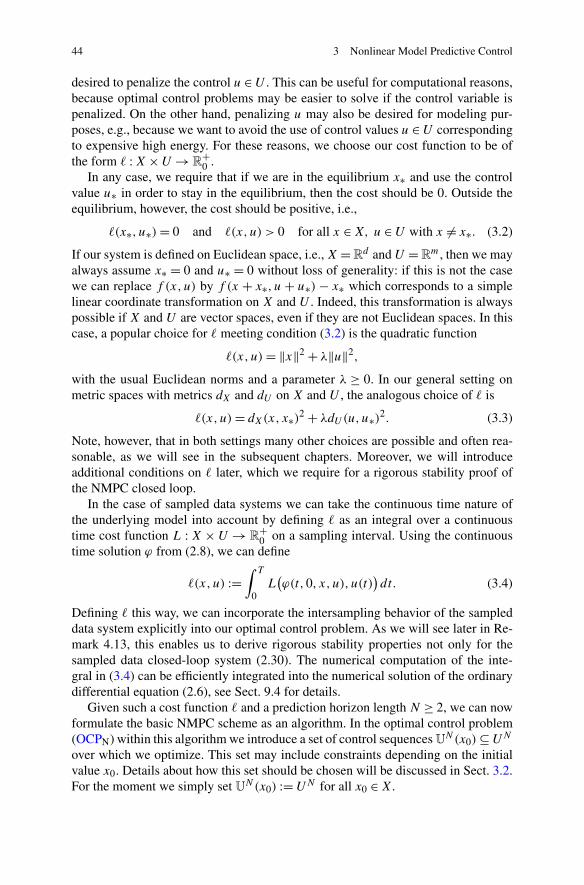
44 3 Nonlinear Model Predictive Control
desired to penalize the control u ∈ U . This can be useful for computational reasons,because optimal control problems may be easier to solve if the control variable ispenalized. On the other hand, penalizing u may also be desired for modeling pur-poses, e.g., because we want to avoid the use of control values u ∈ U correspondingto expensive high energy. For these reasons, we choose our cost function to be ofthe form � : X × U → R
+0 .
In any case, we require that if we are in the equilibrium x∗ and use the controlvalue u∗ in order to stay in the equilibrium, then the cost should be 0. Outside theequilibrium, however, the cost should be positive, i.e.,
�(x∗, u∗) = 0 and �(x,u) > 0 for all x ∈ X, u ∈ U with x �= x∗. (3.2)
If our system is defined on Euclidean space, i.e., X = Rd and U = R
m, then we mayalways assume x∗ = 0 and u∗ = 0 without loss of generality: if this is not the casewe can replace f (x,u) by f (x + x∗, u + u∗) − x∗ which corresponds to a simplelinear coordinate transformation on X and U . Indeed, this transformation is alwayspossible if X and U are vector spaces, even if they are not Euclidean spaces. In thiscase, a popular choice for � meeting condition (3.2) is the quadratic function
�(x,u) = ‖x‖2 + λ‖u‖2,
with the usual Euclidean norms and a parameter λ ≥ 0. In our general setting onmetric spaces with metrics dX and dU on X and U , the analogous choice of � is
�(x,u) = dX(x, x∗)2 + λdU(u,u∗)2. (3.3)
Note, however, that in both settings many other choices are possible and often rea-sonable, as we will see in the subsequent chapters. Moreover, we will introduceadditional conditions on � later, which we require for a rigorous stability proof ofthe NMPC closed loop.
In the case of sampled data systems we can take the continuous time nature ofthe underlying model into account by defining � as an integral over a continuoustime cost function L : X × U → R
+0 on a sampling interval. Using the continuous
time solution ϕ from (2.8), we can define
�(x,u) :=∫ T
0L
(ϕ(t,0, x,u),u(t)
)dt. (3.4)
Defining � this way, we can incorporate the intersampling behavior of the sampleddata system explicitly into our optimal control problem. As we will see later in Re-mark 4.13, this enables us to derive rigorous stability properties not only for thesampled data closed-loop system (2.30). The numerical computation of the inte-gral in (3.4) can be efficiently integrated into the numerical solution of the ordinarydifferential equation (2.6), see Sect. 9.4 for details.
Given such a cost function � and a prediction horizon length N ≥ 2, we can nowformulate the basic NMPC scheme as an algorithm. In the optimal control problem(OCPN) within this algorithm we introduce a set of control sequences U
N(x0) ⊆ UN
over which we optimize. This set may include constraints depending on the initialvalue x0. Details about how this set should be chosen will be discussed in Sect. 3.2.For the moment we simply set U
N(x0) := UN for all x0 ∈ X.

3.2 Constraints 45
Algorithm 3.1 (Basic NMPC algorithm for constant reference xref ≡ x∗) At eachsampling time tn, n = 0,1,2 . . . :
(1) Measure the state x(n) ∈ X of the system.(2) Set x0 := x(n), solve the optimal control problem
minimize JN
(x0, u(·)) :=
N−1∑
k=0
�(xu(k, x0), u(k)
)
with respect to u(·) ∈ UN(x0), subject to
xu(0, x0) = x0, xu(k + 1, x0) = f(xu(k, x0), u(k)
)
(OCPN)
and denote the obtained optimal control sequence by u�(·) ∈ UN(x0).
(3) Define the NMPC-feedback value μN(x(n)) := u�(0) ∈ U and use this controlvalue in the next sampling period.
Observe that in this algorithm we have assumed that an optimal control sequenceu�(·) exists. Sufficient conditions for this existence are briefly discussed after Defi-nition 3.14, below.
The nominal closed-loop system resulting from Algorithm 3.1 is given by (2.5)with state feedback law μ = μN , i.e.,
x+ = f(x,μN(x)
). (3.5)
The trajectories of this system will be denoted by xμN(n) or, if we want to emphasize
the initial value x0 = xμN(0), by xμN
(n, x0).During our theoretical investigations we will neglect the fact that computing the
solution of (OCPN) in Step (2) of the algorithm usually needs some computationtime τc which—in the case when τc is relatively large compared to the samplingperiod T —may not be negligible in a real time implementation. We will sketch asolution to this problem in Sect. 7.6.
In our abstract formulations of the NMPC Algorithm 3.1 only the first elementu�(0) of the respective minimizing control sequence is used in each step, the re-maining entries u�(1), . . . , u�(N −1) are discarded. In the practical implementation,however, these entries play an important role because numerical optimization algo-rithms for solving (OCPN) (or its variants) usually work iteratively: starting froman initial guess u0(·) an optimization algorithm computes iterates ui(·), i = 1,2, . . .
converging to the minimizer u�(·) and a good choice of u0(·) is crucial in order toobtain fast convergence of this iteration, or even to ensure convergence, at all. Here,the minimizing sequence from the previous time step can be efficiently used in orderto construct such a good initial guess. Several different ways to implement this ideaare discussed in Sect. 10.4.
3.2 Constraints
One of the main reasons for the success of NMPC (and MPC in general) is its abil-ity to explicitly take constraints into account. Here, we consider constraints both on
46 3 Nonlinear Model Predictive Control
the control as well as on the state. To this end, we introduce a nonempty state con-straint set X ⊆ X and for each x ∈ X we introduce a nonempty control constraint setU(x) ⊆ U . Of course, U may also be chosen independent of x. The idea behind in-troducing these sets is that we want the trajectories to lie in X and the correspondingcontrol values to lie in U(x). This is made precise in the following definition.
Definition 3.2 Consider a control system (2.1) and the state and control constraintsets X ⊆ X and U(x) ⊆ U .
(i) The states x ∈ X are called admissible states and the control values u ∈ U(x)
are called admissible control values for x.(ii) For N ∈ N and an initial value x0 ∈ X we call a control sequence u ∈ UN and
the corresponding trajectory xu(k, x0) admissible for x0 up to time N , if
u(k) ∈ U(xu(k, x0)
)and xu(k + 1, x0) ∈ X
hold for all k = 0, . . . ,N −1. We denote the set of admissible control sequencesfor x0 up to time N by U
N(x0).(iii) A control sequence u ∈ U∞ and the corresponding trajectory xu(k, x0) are
called admissible for x0 if they are admissible for x0 up to every time N ∈ N.We denote the set of admissible control sequences for x0 by U
∞(x0).(iv) A (possibly time varying) feedback law μ : N0 × X → U is called admissible
if μ(n,x) ∈ U1(x) holds for all x ∈ X and all n ∈ N0.
Whenever the reference to x or x0 is clear from the context we will omit theadditional “for x” or “for x0”.
Since we can (and will) identify control sequences with only one element with therespective control value, we can consider U
1(x0) as a subset of U , which we alreadyimplicitly did in the definition of admissibility for the feedback law μ, above. How-ever, in general U
1(x0) does not coincide with U(x0) ⊆ U because using xu(1, x) =f (x,u) and the definition of U
N(x0) we get U1(x) := {u ∈ U(x) | f (x,u) ∈ X}.
With this subtle difference in mind, one sees that our admissibility condition (iv) onμ ensures both μ(n,x) ∈ U(x) and f (x,μ(n, x)) ∈ X whenever x ∈ X.
Furthermore, our definition of UN(x) implies that even if U(x) = U is indepen-
dent of x the set UN(x) may depend on x for some or all N ∈ N∞.
Often, in order to be suitable for optimization purposes these sets are assumedto be compact and convex. For our theoretical investigations, however, we do notneed any regularity requirements of this type except that these sets are nonempty.We will, however, frequently use the following assumption.
Assumption 3.3 For each x ∈ X there exists u ∈ U(x) such that f (x,u) ∈ X holds.
The property defined in this assumption is called viability or weak (or con-trolled) forward invariance of X. It excludes the situation that there are statesx ∈ X from which the trajectory leaves the set X for all admissible control val-ues. Hence, it ensures U
N(x0) �= ∅ for all x0 ∈ X and all N ∈ N∞. This property is

3.2 Constraints 47
important to ensure the feasibility of (OCPN): the optimal control problem (OCPN)is called feasible for an initial value x0 if the set U
N(x0) over which we optimize isnonempty. Viability of X thus implies that (OCPN) is feasible for each x0 ∈ X andhence ensures that μN(x) is well defined for each x ∈ X. Furthermore, a straight-forward induction shows that under Assumption 3.3 any finite admissible controlsequence u(·) ∈ U
N(x0) can be extended to an infinite admissible control sequenceu(·) ∈ U
∞(x0) with u(k) = u(k) for all k = 0, . . . ,N − 1.In order to see that the construction of a constraint set X meeting Assumption 3.3
is usually a nontrivial task, we reconsider Example 2.2.
Example 3.4 Consider Example 2.2, i.e.,
x+ = f (x,u) =(
x1 + x2 + u/2x2 + u
).
Assume we want to constrain all variables, i.e., the position x1, the velocity x2 andthe acceleration u to the interval [−1,1]. For this purpose one could define X =[−1,1]2 and U(x) = U = [−1,1]. Then, however, for x = (1,1)�, one immediatelyobtains
x+1 = x1 + x2 + u/2 = 2 + u/2 ≥ 3/2
for all u, hence x+ /∈ X for all u ∈ U. Thus, in order to find a viable set X we need toeither tighten or relax some of the constraints. For instance, relaxing the constrainton u to U = [−2,2] the viability of X = [−1,1]2 is guaranteed, because then byelementary computations one sees that for each x ∈ X the control value
u =⎧⎨
⎩
0, x1 + x2 ∈ [−1,1],2 − 2x1 − 2x2, x1 + x2 > 1,
−2 − 2x1 − 2x2, x1 + x2 < −1
is in U and satisfies f (x,u) ∈ X. A way to achieve viability without changing U isby tightening the constraint on x2 by defining
X = {(x1, x2)
T ∈ R2∣∣ x1 ∈ [−1,1], x2 ∈ [−1,1] ∩ [−3/2 − x1,3/2 − x1]
},
(3.6)
see Fig. 3.1. Again, elementary computations show that for each x ∈ X and
u =⎧⎨
⎩
1, x2 < −1/2,
−2x2, x2 ∈ [−1/2,1/2],−1, x2 > 1/2
the desired properties u ∈ U and f (x,u) ∈ X hold.
This example shows that finding viable constraint sets X (and the correspondingU or U(x)) is a tricky task already for very simple systems. Still, Assumption 3.3significantly simplifies the subsequent analysis, cf. Theorem 3.5, below. For thisreason we will impose this condition in our theoretical investigations for schemes

48 3 Nonlinear Model Predictive Control
Fig. 3.1 Illustration of theset X from (3.6)
without stabilizing terminal constraints in Chap. 6. Ways to relax this condition willbe discussed in Sects. 8.1–8.3.
For schemes with stabilizing terminal constraints as featured in Chap. 5 we willnot need this assumption, since for these schemes the region on which the NMPCcontroller is defined is by construction confined to feasible subsets XN of X, seeDefinition 3.9, below. Even if X is not viable, these feasible sets XN turn out tobe viable provided the terminal constraint set is viable, cf. Lemmas 5.2 and 5.10.For a more detailed discussion of these issues see also Part (iv) of the discussion inSect. 8.4.
NMPC is well suited to handle constraints because these can directly be insertedinto Algorithm 3.1. In fact, since we already formulated the corresponding optimiza-tion problem (OCPN) with state dependent control value sets, the constraints arereadily included if we use U
N(x0) from Definition 3.2(ii) in (OCPN). The follow-ing theorem shows that the viability assumption ensures that the NMPC closed-loopsystem obtained this way indeed satisfies the desired constraints.
Theorem 3.5 Consider Algorithm 3.1 using UN(x0) from Definition 3.2(ii) in the
optimal control problem (OCPN) for constraint sets X ⊂ X, U(x) ⊂ U , x ∈ X, sat-isfying Assumption 3.3. Consider the nominal closed-loop system (3.5) and supposethat xμN
(0) ∈ X. Then the constraints are satisfied along the solution of (3.5), i.e.,
xμN(n) ∈ X and μN
(xμN
(n)) ∈ U
(xμN
(n))
(3.7)
for all n ∈ N. Thus, the NMPC-feedback μN is admissible in the sense of Defini-tion 3.2(iv).
Proof First, recall from the discussion after Assumption 3.3 that under this assump-tion the optimal control problem (OCPN) is feasible for each x ∈ X, hence μN(x) iswell defined for each x ∈ X.
We now show that xμN(n) ∈ X implies μN(xμN
(n)) ∈ U(xμN(n)) and xμN
(n +1) ∈ X. Then the assertion follows by induction from xμn(0) ∈ X.
3.2 Constraints 49
The viability of X from Assumption 3.3 ensures that whenever xμN(n) ∈ X
holds in Algorithm 3.1, then x0 ∈ X holds for the respective optimal control prob-lem (OCPN). Since the optimization is performed with respect to admissible con-trol sequences only, also the optimal control sequence u�(·) is admissible forx0 = xμN
(n). This implies μN(xμN(n)) = u�(0) ∈ U
1(xμN(n)) ⊆ U(xμN
(n)) andthus also
xμN(n + 1) = f
(xμN
(n),μN
(xμN
(n))) = f
(x(n),u�(0)
) ∈ X,
i.e., xμN(n + 1) ∈ X. �
Theorem 3.5 in particular implies that if a state x is feasible for (OCPN), whichunder Assumption 3.3 is equivalent to x ∈ X (cf. the discussion after Assump-tion 3.3), then its closed-loop successor state f (x,μN(x)) is again feasible. Thisproperty is called recursive feasibility of X.
In the case of sampled data systems, the constraints are only defined for thesampling times tn but not for the intersampling times t �= tn. That is, for the sampleddata closed-loop system (2.30) we can only guarantee
ϕ(tn, t0, x0,μ) ∈ X for n = 0,1,2, . . .
but in general not
ϕ(t, t0, x0,μ) ∈ X for t �= tn, n = 0,1,2, . . . .
Since we prefer to work within the discrete time framework, directly checkingϕ(t, t0, x0, u) ∈ X for all t does not fit our setting. If desired, however, one couldimplicitly include this condition in the definition of U(x), e.g., by defining newcontrol constraint sets via
U(x) := {u ∈ U(x)
∣∣ ϕ(t,0, x,u) ∈ X for all t ∈ [0, T ]}.In practice, however, this is often not necessary because continuity of ϕ in t ensuresthat the constraints are usually only “mildly” violated for t �= tn, i.e., ϕ(t, t0, x0,μ)
will still be close to X at intersampling times. Still, one should keep this fact in mindwhen designing the constraint set X.
In the underlying optimization algorithms for solving (OCPN), usually the con-straints cannot be specified via sets X and U(x). Rather, one uses so-called equalityand inequality constraints in order to specify X and U(x) according to the followingdefinition.
Definition 3.6 Given functions GSi : X × U → R, i ∈ E S = {1, . . . , pg} and HS
i :X × U → R, i ∈ I S = {pg + 1, . . . , pg + ph} with rg, rh ∈ N0, we define the con-straint sets X and U(x) via
X := {x ∈ X
∣∣ there exists u ∈ U with GSi (x,u) = 0 for all i ∈ E S
and HSi (x,u) ≥ 0 for all i ∈ I S
}
and, for x ∈ X

50 3 Nonlinear Model Predictive Control
U(x) := {u ∈ U
∣∣ GSi (x,u) = 0 for all i ∈ E S and
HSi (x,u) ≥ 0 for all i ∈ I S
}.
Here, the functions GSi and HS
i do not need to depend on both arguments. Thefunctions GS
i , HSi not depending on u are called pure state constraints, the functions
GSi , HS
i not depending on x are called pure control constraints and the functionsGS
i , HSi depending on both x and u are called mixed constraints.
Observe that if we do not have mixed constraints then U(x) is independent of x.The reason for defining X and U(x) via these (in)equality constraints is purely
algorithmic: the plain information “xu(k, x0) /∈ X” does not yield any informationfor the optimization algorithm in order to figure out how to find an admissible u(·),i.e., a u(·) for which “xu(k, x0) ∈ X” holds. In contrast to that, an information ofthe form “HS
i (xu(k, x0), u(k)) < 0” together with additional knowledge about HSi
(provided, e.g., by the derivative of HSi ) enables the algorithm to compute a “direc-
tion” in which u(·) needs to be modified in order to reach an admissible u(·). Formore details on this we refer to Chap. 10.
In our theoretical investigations we will use the notationally more convenientset characterization of the constraints via X and U(x) or U
N(x). In the practicalimplementation of our NMPC method, however, we will use their characterizationvia the inequality constraints from Definition 3.6.
3.3 Variants of the Basic NMPC Algorithms
In this section we discuss some important variants and extensions of the basicNMPC Algorithm 3.1; several further variants will be briefly discussed in Sect. 3.5.We start by incorporating non-constants references xref(n) and afterwards turn toincluding terminal constraints, terminal costs and weights.
If the reference xref is time varying, we need to take this fact into account in theformulation of the NMPC algorithm. Similar to the constant case where we assumedthat x∗ is an equilibrium of (2.1) for control value u∗, we now assume that xref is atrajectory of the system, i.e.,
xref(n) = xuref(n, x0)
for x0 = xref(0) and some suitable admissible reference control sequence uref(·) ∈U
∞(x0). In contrast to the constant reference case of Sect. 3.1, even for X = Rd and
U = Rm we do not assume that these references are constantly equal to 0, because
this would lead to time varying coordinate transformations in X and U . For thisreason, we always need to take xref(·) and uref(·) into account when defining �. As aconsequence, � becomes time varying, too, i.e., we use a function � : N0 ×X×U →R
+0 . Furthermore, we need to keep track of the current sampling instant n in the
optimal control problem.

3.3 Variants of the Basic NMPC Algorithms 51
Again, we require that the cost function � vanishes if and only if we are exactlyon the reference. In the time varying case (3.2) becomes
�(n,xref(n),uref(n)
) = 0 for all n ∈ N0 and
�(n, x,u) > 0 for all n ∈ N0, x ∈ X, u ∈ U with x �= xref(n).(3.8)
For X = Rd , U = R
m with Euclidean norms, a quadratic distance function is nowof the form
�(n, x,u) = ∥∥x − xref(n)
∥∥2 + λ
∥∥u − uref(n)
∥∥2
with λ ≥ 0 and in the general case
�(n, x,u) = dX
(x, xref(n)
)2 + λdU
(u,uref(n)
)2
is an example for � meeting (3.8).For sampled data systems, we can again define � via an integral over a continuous
time cost function L analogous to (3.4). Note, however, that for defining L we willthen need a continuous time reference.
For each k = 0, . . . ,N − 1, the prediction xu(k, x0) with x0 = x(n) used in theNMPC algorithm now becomes a prediction for the closed-loop state x(n+k) whichwe would like to have close to xref(n + k). Consequently, in the optimal controlproblem at time n we need to penalize the distance of xu(k, x0) to xref(n + k),i.e., we need to use the cost �(n + k, xu(k, x0), u(k)). This leads to the followingalgorithm where we minimize over the set of control sequences U
N(x0) defined inSect. 3.2.
Algorithm 3.7 (Basic NMPC algorithm for time varying reference xref) At eachsampling time tn, n = 0,1,2 . . . :
(1) Measure the state x(n) ∈ X of the system.(2) Set x0 = x(n), solve the optimal control problem
minimize JN
(n,x0, u(·)) :=
N−1∑
k=0
�(n + k, xu(k, x0), u(k)
)
with respect to u(·) ∈ UN(x0), subject to
xu(0, x0) = x0, xu(k + 1, x0) = f(xu(k, x0), u(k)
)(OCPn
N)
and denote the obtained optimal control sequence by u�(·) ∈ UN(x0).
(3) Define the NMPC-feedback value μN(n,x(n)) := u�(0) ∈ U and use this con-trol value in the next sampling period.
Note that Algorithm 3.7 and (OCPnN) reduce to Algorithm 3.1 and (OCPN), re-
spectively, if � does not depend on n.The resulting nominal closed-loop system is now given by (2.5) with μ(x) =
μN(n,x), i.e.,
x+ = f(x,μN(n, x)
). (3.9)
52 3 Nonlinear Model Predictive Control
As before, the trajectories of this system will be denoted by xμN(n). Since the right
hand side is now time varying, whenever necessary we include both the initial timeand the initial value in the notation, i.e., for a given n0 ∈ N0 we write xμN
(n,n0, x0)
for the closed-loop solution satisfying xμN(n0, n0, x0) = x0. It is straightforward to
check that Theorem 3.5 remains valid for Algorithm 3.7 when (3.7) is replaced by
xμN(n) ∈ X and μN
(n,xμN
(n)) ∈ U
(xμN
(n)). (3.10)
Remark 3.8 Observe that Algorithm 3.7 can be straightforwardly extended to thecase when f and X depend on n, too. However, in order to keep the presentationsimple, we do not explicitly reflect this possibility in our notation.
More often than not one can find variations of the basic NMPC Algorithms 3.1and 3.7 in the literature in which the optimal control problem (OCPN) or (OCPn
N)is changed in one way or another in order to improve the closed-loop performance.These techniques will be discussed in detail in Chap. 5 and in Sects. 7.1 and 7.2.We now introduce generalizations (OCPN,e) and (OCPn
N,e) of (OCPN) and (OCPnN),
respectively, which contain all the variants we will investigate in these chapters andsections.
A typical choice for such a variant is an additional terminal constraint of the form
xu
(N,x(n)
) ∈ X0 for a terminal constraint set X0 ⊆ X (3.11)
for the time-invariant case of (OCPN) and
xu
(N,x(n)
) ∈ X0(n + N) for terminal constraint sets X0(n) ⊆ X, n ∈ N0
(3.12)
for the time varying problem (OCPnN). Of course, in the practical implementation
the constraint sets X0 or X0(n) are again expressed via (in)equalities of the formgiven in Definition 3.6.
When using terminal constraints, the NMPC-feedback law is only defined forthose states x0 for which the optimization problem within the NMPC algorithm isfeasible also for these additional constraints, i.e., for which there exists an admissi-ble control sequence with corresponding trajectory starting in x0 and ending in theterminal constraint set. Such initial values are again called feasible and the set of allfeasible initial values form the feasible set. This set along with the correspondingadmissible control sequences is formally defined as follows.
Definition 3.9
(i) For X0 from (3.11) we define the feasible set for horizon N ∈ N by
XN := {x0 ∈ X
∣∣ there exists u(·) ∈ UN(x0) with xu(N,x0) ∈ X0
}
and for each x0 ∈ XN we define the set of admissible control sequences by
UNX0
(x0) := {u(·) ∈ U
N(x0)∣∣ xu(N,x0) ∈ X0
}.

3.3 Variants of the Basic NMPC Algorithms 53
(ii) For X0(n) from (3.12) we define the feasible set for horizon N ∈ N at timen ∈ N0 by
XN(n) := {x0 ∈ X
∣∣ there exists u(·) ∈ UN(x0) with xu(N,x0) ∈ X0(n + N)
}
and for each x0 ∈ XN(n) we define the set of admissible control sequences by
UNX0
(n, x0) := {u(·) ∈ U
N(x0)∣∣ xu(N,x0) ∈ X0(n + N)
}.
Note that in (i) XN = X and UNX0
(x) = UN(x) holds if X0 = X, i.e., if no ad-
ditional terminal constraints are imposed. Similarly, in case (ii) XN(n) = X andU
NX0
(n, x) = UN(x) holds if X0(n) = X.
Another modification of the optimal control problems (OCPN) and (OCPnN),
often used in conjunction with this terminal constraint is an additional termi-nal cost of the form F(xu(N,x(n))) with F : X → R
+0 in the optimization ob-
jective. This function may also be time depending, i.e., it may be of the formF(n + N,xu(N,x(n))) with F : N0 × X → R
+0 . An alternative to using ter-
minal costs is to put weights on some summands of the objective, i.e., replac-ing �(xu(k, x0), u(k)) by ωN−k�(xu(k, x0), u(k)) for weights ω1, . . . ,ωN ≥ 0. Al-though for NMPC schemes we will only investigate the effect of the weight ω1in detail, cf. Sect. 7.2, here we introduce weights for all summands since this of-fers more flexibility and does not further complicate the subsequent analysis in thischapter. The need for the “backward” numbering of the ωN−k will become clear inthe proof of Theorem 3.15, below.
In the sequel, we will analyze schemes with terminal cost F and schemes withweights ωN−k separately, cf. Sects. 5.3, 7.1 and 7.2. However, in order to reduce thenumber of variants of NMPC algorithms in this book we include both features in theoptimization problems (OCPN,e) and (OCPn
N,e) in the following NMPC algorithmsextending the basic Algorithms 3.1 and 3.7, respectively. Note that compared tothese basic algorithms only the optimal control problems are different, i.e., the partin the boxes in Step (2). We start by extending the time-invariant Algorithm 3.1
Algorithm 3.10 (Extended NMPC algorithm for constant reference xref ≡ x∗) Ateach sampling time tn, n = 0,1,2 . . . :
(1) Measure the state x(n) ∈ X of the system.(2) Set x0 := x(n), solve the optimal control problem
minimize JN
(x0, u(·)) :=
N−1∑
k=0
ωN−k�(xu(k, x0), u(k)
)
+ F(xu(N,x0)
)
with respect to u(·) ∈ UNX0
(x0), subject to
xu(0, x0) = x0, xu(k + 1, x0) = f(xu(k, x0), u(k)
)
(OCPN,e)
and denote the obtained optimal control sequence by u�(·) ∈ UNX0
(x0).

54 3 Nonlinear Model Predictive Control
(3) Define the NMPC-feedback value μN(x(n)) := u�(0) ∈ U and use this controlvalue in the next sampling period.
Similarly, we can extend the time-variant Algorithm 3.7.
Algorithm 3.11 (Extended NMPC algorithm for time varying reference xref) Ateach sampling time tn, n = 0,1,2 . . . :
(1) Measure the state x(n) ∈ X of the system.(2) Set x0 = x(n), solve the optimal control problem
minimize JN
(n,x0, u(·)) :=
N−1∑
k=0
ωN−k�(n + k, xu(k, x0), u(k)
)
+ F(n + N,xu(N,x0)
)
with respect to u(·) ∈ UNX0
(n, x0), subject to
xu(0, x0) = x0, xu(k + 1, x0) = f(xu(k, x0), u(k)
)
(OCPnN,e)
and denote the obtained optimal control sequence by u�(·) ∈ UNX0
(n, x0).(3) Define the NMPC-feedback value μN(n,x(n)) := u�(0) ∈ U and use this con-
trol value in the next sampling period.
Observe that the terminal constraints (3.11) and (3.12) are included via the re-strictions u(·) ∈ U
NX0
(x0) and u(·) ∈ UNX0
(n, x0), respectively.Algorithm 3.10 is a special case of Algorithm 3.11 if �, F and X0 do not de-
pend on n. Furthermore, Algorithm 3.1 is obtained from Algorithm 3.10 for F ≡ 0,ωNk
= 1, k = 0, . . . ,N − 1 and X0 = X. Likewise, we can derive Algorithm 3.7from Algorithm 3.11 by setting F ≡ 0, ωNk
= 1, k = 0, . . . ,N − 1 and X0(n) = X,n ∈ N0. Consequently, all NMPC algorithms in this book are special cases of Algo-rithm 3.11 and all optimal control problems included in these algorithms are specialcases of (OCPn
N,e).We end this section with two useful results on the sets of admissible control
sequences from Definition 3.9 which we formulate for the general setting of Algo-rithm 3.11, i.e., for time varying terminal constraint set X0(n).
Lemma 3.12 Let x0 ∈ XN(n), N ∈ N and K ∈ {0, . . . ,N} be given.
(i) For each u(·) ∈ UNX0
(n, x0) we have xu(K,x0) ∈ XN−K(n + K).
(ii) For each u(·) ∈ UNX0
(n, x0) the control sequences u1 ∈ UK and u2 ∈ UN−K
uniquely defined by the relation
u(k) ={
u1(k), k = 0, . . . ,K − 1,
u2(k − K), k = K, . . . ,N − 1(3.13)
satisfy u1 ∈ UKXN−K
(n, x0) and u2 ∈ UN−KX0
(n + K,xu1(K,x0)).

3.3 Variants of the Basic NMPC Algorithms 55
(iii) For each u1(·) ∈ UKXN−K
(n, x0) there exists u2(·) ∈ UN−KX0
(n + K,xu1(K,x0))
such that u(·) from (3.13) satisfies u ∈ UNX0
(n, x0).
Proof (i) Using (2.3) we obtain the identity
xu(K+·)(N − K,xu(K,x0)
) = xu(N,x0) ∈ X0(n + N),
which together with the definition of XN−K implies the assertion.(ii) The relation (3.13) together with (2.3) implies
xu(k, x0) ={
xu1(k, x0), k = 0, . . . ,K ,
xu2(k − K,xu1(K,x0)), k = K, . . . ,N .(3.14)
For k = 0, . . . ,K − 1 this identity and (3.13) yield
u1(k) = u(k) ∈ U(xu(k, x0)
) = U(xu1(k, x0)
)
and for k = 0, . . . ,N − K − 1 we obtain
u2(k) = u(k + K) ∈ U(xu(k + K,x0)
) = U(xu2
(k, xu1(K,x0)
)),
implying u1 ∈ UK(x0) and u2 ∈ U
N−K(xu1(K,x0)). Furthermore, (3.14) impliesthe equation xu2(N − K,xu1(K,x0)) = xu(N,x0) ∈ X0(n + N) which proves u2 ∈U
N−KX0
(n + K,xu1(K,x0)). This, in turn, implies that UN−KX0
(n + K,xu1(K,x0)) is
nonempty, hence xu1(K,x0) ∈ XN−K(n+K) and consequently u1 ∈ UKXN−K
(n, x0)
follows.(iii) By definition, for each x ∈ XN−K(n+K) there exists u2 ∈ U
N−KX0
(n+K,x).Choosing such a u2 for x = xu1(K,x0) ∈ XN−K(n + K) and defining u via (3.13),similar arguments as in Part (ii), above, show the claim u ∈ U
NX0
(n, x0). �
A straightforward corollary of this lemma is the following.
Corollary 3.13
(i) For each x ∈ XN the NMPC-feedback law μN obtained from Algorithm 3.10satisfies
f(x,μN(x)
) ∈ XN−1.
(ii) For each n ∈ N and each x ∈ XN(n) the NMPC-feedback law μN obtained fromAlgorithm 3.11 satisfies
f(x,μN(n, x)
) ∈ XN−1(n + 1).
Proof We show (ii) which contains (i) as a special case. Since μN(n,x) isthe first element u�(0) of the optimal control sequence u� ∈ U
NX0
(n, x) we getf (x,μN(n, x)) = xu�(1, x). Now Lemma 3.12(i) yields the assertion. �
56 3 Nonlinear Model Predictive Control
3.4 The Dynamic Programming Principle
In this section we provide one of the classical tools in optimal control, the dynamicprogramming principle. We will formulate and prove the results in this section for(OCPn
N,e), since all other optimal control problems introduced above can be ob-tained a special cases of this problem. We will first formulate the principle forthe open-loop control sequences in (OCPn
N,e) and then derive consequences for theNMPC-feedback law μN . The dynamic programming principle is often used as abasis for numerical algorithms, cf. Sect. 3.5. In contrast to this, in this book wewill exclusively use the principle for analyzing the behavior of NMPC closed-loopsystems, while for the actual numerical solution of (OCPn
N,e) we use different al-gorithms as described in Chap. 10. The reason for this is that the numerical effortof solving (OCPn
N,e) via dynamic programming usually grows exponentially withthe dimension of the state of the system, see the discussion in Sect. 3.5. In contrastto this, the computational effort of the methods described in Chap. 10 scales muchmore moderately with the space dimension.
We start by defining some objects we need in the sequel.
Definition 3.14 Consider the optimal control problem (OCPnN,e) with initial value
x0 ∈ X, time instant n ∈ N0 and optimization horizon N ∈ N0.
(i) The function
VN(n, x0) := infu(·)∈U
NX0
(x0)
JN
(n,x0, u(·))
is called optimal value function.(ii) A control sequence u�(·) ∈ U
NX0
(x0) is called optimal control sequence for x0,if
VN(n, x0) = JN
(n,x0, u
�(·))
holds. The corresponding trajectory xu�(·, x0) is called optimal trajectory.
In our NMPC Algorithm 3.11 and its variants we have assumed that an optimalcontrol sequence u�(·) exists, cf. the comment after Algorithms 3.1. In general, thisis not necessarily the case but under reasonable continuity and compactness condi-tions the existence of u�(·) can be rigorously shown. Examples of such theorems fora general infinite-dimensional state space can be found in Keerthi and Gilbert [10]or Doležal [7]. While for formulating and proving the dynamic programming princi-ple we will not need the existence of u�(·), for all subsequent results we will assumethat u�(·) exists, in particular when we derive properties of the NMPC-feedback lawμN . While we conjecture that most of the results in this book can be generalized tothe case when μN is defined via an approximately minimizing control sequence,we decided to use the existence assumption because it considerably simplifies thepresentation of the results in this book.
The following theorem introduces the dynamic programming principle. It givesan equation which relates the optimal value functions for different optimization hori-zons N and for different points in space.

3.4 The Dynamic Programming Principle 57
Theorem 3.15 Consider the optimal control problem (OCPnN,e) with x0 ∈ XN(n)
and n,N ∈ N0. Then for all N ∈ N and all K = 1, . . . ,N the equation
VN(n, x0) = infu(·)∈U
KXN−K
(n,x0)
{K−1∑
k=0
ωN−k�(n + k, xu(k, x0), u(k)
)
+ VN−K
(n + K,xu(K,x0)
)}
(3.15)
holds. If, in addition, an optimal control sequence u�(·) ∈ UNX0
(n, x0) exists for x0,then we get the equation
VN(n, x0) =K−1∑
k=0
ωN−k�(n + k, xu�(k, x0), u
�(k)) + VN−K
(n + K,xu�(K,x0)
).
(3.16)
In particular, in this case the “inf” in (3.15) is a “min”.
Proof First observe that from the definition of JN for u(·) ∈ UNX0
(n, x0) we imme-diately obtain
JN
(n,x0, u(·)) =
K−1∑
k=0
ωN−k�(n + k, xu(k, x0), u(k)
)
+ JN−K
(n + K,xu(K,x0), u(· + K)
). (3.17)
Since u(· + K) equals u2(·) from Lemma 3.12(ii) we obtain u(· + K) ∈ UN−KX0
(n +K,xu(K,x0)). Note that for (3.17) to hold we need the backward numbering ofωN−k .
We now prove (3.15) by proving “≥” and “≤” separately. From (3.17) we obtain
JN
(n,x0, u(·)) =
K−1∑
k=0
ωN−k�(n + k, xu(k, x0), u(k)
)
+ JN−K
(n + K,xu(K,x0), u(· + K)
)
≥K−1∑
k=0
ωN−k�(n + k, xu(k, x0), u(k)
) + VN−K
(n + K,xu(K,x0)
).
Since this inequality holds for all u(·) ∈ UNX0
(n, x0), it also holds when taking theinfimum on both sides. Hence we get
VN(n, x0) = infu(·)∈U
NX0
(n,x0)
JN
(n,x0, u(·))
≥ infu(·)∈U
NX0
(n,x0)
{K−1∑
k=0
ωN−k�(n + k, xu(k, x0), u(k)
)
58 3 Nonlinear Model Predictive Control
+ VN−K
(n + K,xu(K,x0)
)}
= infu1(·)∈U
KXN−K
(n,x0)
{K−1∑
k=0
ωN−k�(n + k, xu1(k, x0), u(k)
)
+ VN−K
(n + K,xu1(K,x0)
)}
,
i.e., (3.15) with “≥”. Here in the last step we used the fact that by Lemma 3.12(ii) thecontrol sequence u1 consisting of the first K elements of u(·) ∈ U
NX0
(n, x0) lies in
UKXN−K
(n, x0) and, conversely, by Lemma 3.12(iii) each control sequence in u1(·) ∈U
KXN−K
(n, x0) can be extended to a sequence in u(·) ∈ UNX0
(n, x0). Thus, since theexpression in braces does not depend on u(K), . . . , u(N − 1), the infima coincide.
In order to prove “≤”, fix ε > 0 and let uε(·) be an approximately optimal controlsequence for the right hand side of (3.17), i.e.,
K−1∑
k=0
ωN−k�(n + k, xuε (k, x0), u
ε(k)) + JN−K
(n + K,xuε (K,x0), u
ε(· + K))
≤ infu(·)∈U
NX0
(n,x0)
{K−1∑
k=0
ωN−k�(n + k, xu(k, x0), u(k)
)
+ JN−K
(n + K,xu(K,x0), u(· + K)
)}
+ ε.
Now we use the decomposition (3.13) of u(·) into u1 ∈ UKXN−K
(n, x0) and u2 ∈U
N−KX0
(n + K,xu1(K,x0)) from Lemma 3.12(ii). This way we obtain
infu(·)∈U
NX0
(n,x0)
{K−1∑
k=0
ωN−k�(n + k, xu(k, x0), u(k)
)
+ JN−K
(n + K,xu(K,x0), u(· + K)
)}
= infu1(·)∈U
KXN−K
(n,x0)
u2(·)∈UN−KX0
(n+K,xu1 (K,x0))
{K−1∑
k=0
ωN−k�(n + k, xu1(k, x0), u1(k)
)
+ JN−K
(n + K,xu1(K,x0), u2(·)
)}
= infu1(·)∈U
KXN−K
(n,x0)
{K−1∑
k=0
ωN−k�(n + k, xu1(k, x0), u1(k)
)

3.4 The Dynamic Programming Principle 59
+ VN−K
(n + K,xu1(K,x0)
)}
.
Now (3.17) yields
VN(n, x0) ≤ JN
(n,x0, u
ε(·))
=K−1∑
k=0
ωN−k�(n + k, xuε (k, x0), u
ε(k))
+ JN−K
(n + K,xuε (K,x0), u
ε(· + K))
≤ infu(·)∈U
KXN−K
(n,x0)
{K−1∑
k=0
ωN−k�(n + k, xu(k, x0), u(k)
)
+ VN−K
(n + K,xu(K,x0)
)}
+ ε.
Since the first and the last term in this inequality chain are independent of ε andsince ε > 0 was arbitrary, this shows (3.15) with “≤” and thus (3.15).
In order to prove (3.16) we use (3.17) with u(·) = u�(·). This yields
VN(n, x0) = JN
(n,x0, u
�(·))
=K−1∑
k=0
ωN−k�(n + k, xu�(k, x0), u
�(k))
+ JN−K
(n + K,xu�(K,x0), u
�(· + K))
≥K−1∑
k=0
ωN−k�(n + k, xu�(k, x0), u
�(k)) + VN−K
(n + K,xu�(K,x0)
)
≥ infu(·)∈U
KXN−K
(n,x0)
{K−1∑
k=0
ωN−k�(n + k, xu(k, x0), u(k)
)
+ VN−K
(n + K,xu(K,x0)
)}
= VN(n, x0),
where we used the (already proven) Equality (3.15) in the last step. Hence, the two“≥” in this chain are actually “=” which implies (3.16). �
The following corollary states an immediate consequence of the dynamic pro-gramming principle. It shows that tails of optimal control sequences are again opti-mal control sequences for suitably adjusted optimization horizon, time instant andinitial value.

60 3 Nonlinear Model Predictive Control
Corollary 3.16 If u�(·) is an optimal control sequence for initial value x0 ∈ XN(n),time instant n and optimization horizon N ≥ 2, then for each K = 1, . . . ,N − 1 thesequence u�
K(·) = u�(· + K), i.e.,
u�K(k) = u�(K + k), k = 0, . . . ,N − K − 1
is an optimal control sequence for initial value xu�(K,x0), time instant n + K andoptimization horizon N − K .
Proof Inserting VN(n, x0) = JN(n, x0, u�(·)) and the definition of u�
k(·) into (3.17)we obtain
VN(n, x0) =K−1∑
k=0
ωN−k�(n + k, xu�(k, x0), u
�(k))
+ JN−K
(n + K,xu�(K,x0), u
�K(·)).
Subtracting (3.16) from this equation yields
0 = JN−K
(n + K,xu�(K,x0), u
�K(·)) − VN−K
(n + K,xu�(K,x0)
)
which shows the assertion. �
The next theorem relates the NMPC-feedback law μN defined in the NMPCAlgorithm 3.11 and its variants to the dynamic programming principle. Here we usethe argmin operator in the following sense: for a map a : U → R, a nonempty subsetU ⊆ U and a value u� ∈ U we write
u� = argminu∈U
a(u) (3.18)
if and only if a(u�) = infu∈U a(u) holds. Whenever (3.18) holds the existence of theminimum minu∈U a(u) follows. However, we do not require uniqueness of the mini-mizer u�. In case of uniqueness equation (3.18) can be understood as an assignment,otherwise it is just a convenient way of writing “u� minimizes a(u)”.
Theorem 3.17 Consider the optimal control problem (OCPnN,e) with x0 ∈ XN(n)
and n,N ∈ N0 and assume that an optimal control sequence u� exists. Then theNMPC-feedback law μN(n,x0) = u∗(0) satisfies
μN(n,x0) = argminu∈U
1XN−1
(n,x0)
{ωN�(n, x0, u) + VN−1
(n + 1, f (x0, u)
)}(3.19)
and
VN(n, x0) = ωN�(n,x0,μN(n, x0)
) + VN−1(n + 1, f
(x0,μN(n, x0)
))(3.20)
where in (3.19) we interpret U1XN−1
(n, x0) as a subset of U , i.e., we identify the oneelement sequence u = u(·) with its only element u = u(0).

3.4 The Dynamic Programming Principle 61
Proof Equation (3.20) follows by inserting u�(0) = μN(n,x0) and xu�(1, x0) =f (x0,μN(n, x0)) into (3.16) for K = 1.
Inserting xu(1, x0) = f (x0, u) into the dynamic programming principle (3.15)for K = 1 we further obtain
VN(n, x0) = infu∈U
1XN−1
(n,x0)
{ωN�(n, x0, u) + VN−1
(n + 1, f (x0, u)
)}. (3.21)
This implies that the right hand sides of (3.20) and (3.21) coincide. Thus, the defi-nition of argmin in (3.18) with a(u) = ωN�(n, x0, u) + VN−1(n + 1, f (x0, u)) andU = U
1XN−1
(n, x0) yields (3.19). �
Our final corollary in this section shows that we can reconstruct the whole opti-mal control sequence u�(·) using the feedback from (3.19).
Corollary 3.18 Consider the optimal control problem (OCPnN,e) with x0 ∈ X and
n,N ∈ N0 and consider admissible feedback laws μN−k : N0 × X → U , k =0, . . . ,N − 1, in the sense of Definition 3.2(iv). Denote the solution of the closed-loop system
x(0) = x0,
x(k + 1) = f(x(k),μN−k
(n + k, x(k)
)), k = 0, . . . ,N − 1 (3.22)
by xμ(·) and assume that the μN−k satisfy (3.19) with horizon N − k instead of N ,time index n + k instead of n and initial value x0 = xμ(k) for k = 0, . . . ,N − 1.Then
u�(k) = μN−k
(n + k, xμ(k)
), k = 0, . . . ,N − 1 (3.23)
is an optimal control sequence for initial time n and initial value x0 and the solutionof the closed-loop system (3.22) is a corresponding optimal trajectory.
Proof Applying the control (3.23) to the dynamics (3.22) we immediately obtain
xu�(n, x0) = xμ(n), n = 0, . . . ,N − 1.
Hence, we need to show that
VN(n, x0) = JN
(n,x0, u
�) =
N−1∑
k=0
ωN−k�(n + k, x(k), u�(k)
) + F(n + N,x(N)
).
Using (3.23) and (3.20) for N − k instead of N we get
VN−k(n + k, x0) = ωN−k�(n + k, x(k), u�(k)
) + VN−k−1(n + k + 1, x(k + 1)
)
for k = 0, . . . ,N −1. Summing these equalities for k = 0, . . . ,N −1 and eliminatingthe identical terms VN−k(n + k, x0), k = 1, . . . ,N − 1 on both sides we obtain
VN(n, x0) =N−1∑
k=0
ωN−k�(n + k, x(k), u�(k)
) + V0(n + N,x(N)
).
Since by definition of J0 we have V0(n + N,x) = F(n + N,x), this shows theassertion. �

62 3 Nonlinear Model Predictive Control
3.5 Notes and Extensions
The discrete time nonlinear model predictive control framework introduced inSects. 3.1–3.3 covers most of the settings commonly found in the literature. Forcontinuous time systems, one often also finds nonlinear model predictive controlframeworks in explicit continuous time form. In these frameworks, the optimiza-tion in (OCPn
N,e) and its variants is carried out at times t0, t1, t2, . . . minimizing anintegral criterion along the continuous time solution of the form
JTopt(x0, v) =∫ Topt
0L
(ϕ(t, x0, v), v(t)
)dt + F
(ϕ(Topt,N,x0, v)
).
The feedback law μTopt computed at time tn is then obtained by applying the firstportion v�|[0,tn+1−tn] of the optimal control function v� to the system, see, e.g.,Alamir [1] or Findeisen [9]. Provided that tn+1 − tn = T holds for all n, this problemis equivalent to our setting if the sampled data system (2.8) and the integral criterion(3.4) is used.
Regarding notation, in NMPC it is important to distinguish between the open-loop predictions and the NMPC closed loop. Here we have decided to denote theopen-loop predictions by xu(k) or xu(k, x0) and the NMPC closed-loop trajecto-ries by either x(n) or—more often—by xμN
(n) or xμN(n, x0). There are, however,
various other notations commonly found in the literature. For instance, the predic-tion at time instant n is occasionally denoted as x(k|n) in order to emphasize thedependence on the time instant n. In our notation, the dependence on n is implic-itly expressed via the initial condition x0 = x(n) and the index n in (OCPn
N) or(OCPn
N,e). Whenever necessary, the value of n under consideration will be specifiedin the context. On the other hand, we decided to always explicitly indicate the de-pendence of open-loop solutions on the control sequence u. This notation enablesus to easily distinguish between open-loop and closed-loop solutions and also forsimultaneously considering open-loop solutions for different control sequences.
In linear discrete time MPC, the optimization at each sampling instant is oc-casionally performed over control sequences with predefined values u(K), . . . ,
u(N −1) for some K ∈ {1, . . . ,N −1}, i.e., only u(0), . . . , u(K −1) are used as op-timization variables in (OCPN,e) and its variants. For instance, if x∗ = 0 and u∗ = 0,cf. Sect. 3.1, then u(K), . . . , u(N − 1) = 0 is a typical choice. In this setting, K
is referred to as optimization horizon (or control horizon) and N is referred to asprediction horizon. Since this variant is less common in nonlinear MPC, we do notconsider it in this book; in particular, we use the terms optimization horizon andprediction horizon synonymously, while the term control horizon will receive a dif-ferent meaning in Sect. 7.4. Still, most of the subsequent analysis could be extendedto the case in which the optimization horizon and the prediction horizon do notcoincide.
Regarding the cost function �, the setting described in Sects. 3.1 and 3.3 is easilyextended to the case in which a set instead of a single equilibrium or a time-variantfamily of sets instead of a single reference shall be stabilized. Indeed, if we are given

3.5 Notes and Extensions 63
a family of sets Xref(n) ⊂ X such that for each x ∈ Xref(n) there is a control ux withf (x,ux) ∈ Xref(n + 1), then we can modify (3.8) to
�(n, x,ux) = 0 for all x ∈ Xref(n) and
�(n, x,u) > 0 for all x ∈ X \ Xref(n), u ∈ U.(3.24)
Similarly, we can modify (3.2) in the time-invariant case.Another modification of �, again often found in the linear MPC literature,
are running cost functions which include two consecutive control values, i.e.,�(xu(k), u(k), u(k − 1)). Typically, this is used in order to penalize large changesin the control input by adding a term σ‖u(k) − u(k − 1)‖ (assuming U to be avector space with norm ‖ · ‖, for simplicity). Using the augmented state xu(k) =(xu(k), u(k − 1)) this can be transformed into a cost function meeting our setting bydefining �(xu(k), u(k)) = �(xu(k), u(k), u(k − 1)).
Yet another commonly used variant are running costs in which only an outputy = h(x) instead of the whole state is taken into account. In this case, � will usuallyno longer satisfy (3.2) or (3.8), i.e., � will not be positive definite, anymore. Wewill discuss this case in Sect. 7.3. In this context it should be noted that even if therunning cost � depends only on an output, the NMPC-feedback μN will neverthelessbe a state feedback law. Hence, if only output data is available, suitable observersneed to be used in order to reconstruct the state of the system.
The term dynamic programming was introduced by Bellman [2] and due to hisseminal contributions to this area the dynamic programming principle is often alsocalled Bellman’s principle of optimality. The principle is widely used in many ap-plication areas and a quite comprehensive account of its use in various differentsettings is given in the monographs by Bertsekas [4, 5]. For K = 1, the dynamicprogramming principle (3.15) simplifies to
VN(n, x) = infu∈U
1XN−1
(n,x)
{ωN�(n + k, x,u) + VN−1
(n + 1, f (x,u)
)}(3.25)
and in this form it can be used for recursively computing V1,V2, . . . , VN startingfrom V0(n, x) = F(n,x). Once VN and VN−1 are known, the feedback law μN canbe obtained from (3.19).
Whenever VN can be expressed using simple functions this approach of comput-ing VN can be efficiently used. For instance, when the dynamics are linear and finitedimensional, the running cost is quadratic and there are no constraints, then VN canbe expressed as VN(x) = x�PNx for a matrix PN ∈ R
d×d and (3.25) reduces to theRiccati difference equation, see, e.g., Dorato and Levis [8].
For nonlinear systems with low-dimensional state space it is also possible toapproximate VN numerically using the backward recursion induced by (3.25) withapproximations V1 ≈ V1, . . . , VN ≈ VN . These approximations can then, in turn, beused in order to compute a numerical approximation of the NMPC-feedback lawμN . This is, roughly speaking, the idea behind the so-called explicit MPC methods,see, e.g., Borrelli, Baotic, Bemporad and Morari [6], Bemporad and Filippi [3],Tøndel, Johansen and Bemporad [11], to mention but a few papers from this areain which often special problem structures like piecewise linear dynamics instead of

64 3 Nonlinear Model Predictive Control
general nonlinear models are considered. The main advantage of this approach isthat VN and the approximation of μN can be computed offline and thus the onlinecomputational effort of evaluating μN is very low. Hence, in contrast to conventionalNMPC in which (OCPn
N,e) is entirely solved online, this method is also applicableto very fast systems which require fast sampling.
Unfortunately, for high-dimensional systems, the numerical effort of this ap-proach becomes prohibitive since the computational complexity of computing VN
grows exponentially in the state dimension, unless one can exploit very specificproblem structure. This fact—the so-called curse of dimensionality—arises becausethe approximation of VN requires a global solution to (OCPn
N,e) or its variants for allinitial values x0 ∈ X or at least in the set of interest, which is typically a set of fulldimension in state space. Consequently, the dynamic programming method cannotbe applied to high-dimensional systems. In contrast to this, the methods we will dis-cuss in Chap. 10 solve (OCPn
N,e) for a single initial value x0 only at each samplinginstant, i.e. locally in space. Since this needs to be done online, these methods are inprinciple slower, but since the numerical effort scales much more moderate with thestate dimension they are nevertheless applicable to systems with much higher statedimension.
3.6 Problems
1. Consider the control system
x+ = f (x,u) = ax + bu
with x ∈ X = R, u ∈ U = R, constraints X = [−1,1] and U = [−100,100] andreal parameters a, b ∈ R.(a) For which parameters a, b ∈ R is the state constraint set X viable?(b) For those parameters for which X is not viable, determine a viable state
constraint set contained in X.2. Compute an optimal trajectory for the optimal control problem (OCPN,e)
minimizeN−1∑
k=0
u(k)2,
subject to x1(k + 1) = x1(k) + 2x2(k),
x2(k + 1) = 2u(k) − x2(k),
x1(0) = 0, x2(0) = 0,
x1(N) = 4, x2(N) = 0
with N = 4 via dynamic programming.3. Consider the NMPC problem defined by the dynamics
x+ = f (x,u) = x + u
References 65
with x ∈ X = R, u ∈ U = R and running costs
�(x,u) = x2 + u2.
(a) Compute the optimal value function V2 and the NMPC-feedback law μ2 bydynamic programming.
(b) Show that V2 is a Lyapunov function for the closed loop and compute thefunctions α1, α2 and αV in (2.37) and (2.38).
(c) Show that the NMPC closed loop is globally asymptotically stable withoutusing the Lyapunov function V2.
4. Consider an optimal trajectory xu�(·, x0) for the optimal control problem (OCPN)with initial value x0 and optimization horizon N ≥ 2. Prove that for any K ∈{1, . . . ,N − 1} the tail
xu�(K,x0), . . . , xu�(N − 1, x0)
of the optimal trajectory along with the tail
u�(K), . . . , u�(N − 1)
of the optimal control sequence are optimal for (OCPN) with new initial valuexu�(K,x0) and optimization horizon N − K , i.e., that
N−1∑
k=K
�(xu�(k, x0), u
�(k)) = VN−K
(xu�(K,x0)
)
holds.5. After a lecture in which you presented the basic NMPC Algorithm 3.1, a student
asks the following question:“If I ride my bicycle and want to make a turn to the left, I first steer a little
bit to the right to make my bicycle tilt to the left. Let us assume that this wayof making a turn is optimal for a suitable problem of type (OCPN). This wouldmean that the optimal control sequence will initially steer to the right and latersteer to the left. If we use this optimal control sequence in an NMPC algorithm,only the first control action will be implemented. As a consequence, we willalways steer to the right, and we will make a turn to the right instead of a turn tothe left. Does this mean that NMPC does not work for controlling my bicycle?”
What do you respond?
References
1. Alamir, M.: Stabilization of Nonlinear Systems Using Receding-horizon Control Schemes.Lecture Notes in Control and Information Sciences, vol. 339. Springer, London (2006)
2. Bellman, R.: Dynamic Programming. Princeton University Press, Princeton (1957). Reprintedin 2010
3. Bemporad, A., Filippi, C.: Suboptimal explicit MPC via approximate multiparametricquadratic programming. In: Proceedings of the 40th IEEE Conference on Decision and Con-trol – CDC 2001, Orlando, Florida, USA, pp. 4851–4856 (2001)

66 3 Nonlinear Model Predictive Control
4. Bertsekas, D.P.: Dynamic Programming and Optimal Control, vol. I, 3rd edn. Athena Scien-tific, Belmont (2005)
5. Bertsekas, D.P.: Dynamic Programming and Optimal Control, vol. II, 2nd edn. Athena Scien-tific, Belmont (2001)
6. Borrelli, L., Baotic, T., Bemporad, A., Morari, T.: Efficient on-line computation of constrainedoptimal control. In: Proceedings of the 40th IEEE Conference on Decision and Control – CDC2001, Orlando, Florida, USA, pp. 1187–1192 (2001)
7. Doležal, J.: Existence of optimal solutions in general discrete systems. Kybernetika 11(4),301–312 (1975)
8. Dorato, P., Levis, A.H.: Optimal linear regulators: the discrete-time case. IEEE Trans. Au-tomat. Control 16, 613–620 (1971)
9. Findeisen, R.: Nonlinear model predictive control: a sampled-data feedback perspective. PhDthesis, University of Stuttgart, VDI-Verlag, Düsseldorf (2004)
10. Keerthi, S.S., Gilbert, E.G.: An existence theorem for discrete-time infinite-horizon optimalcontrol problems. IEEE Trans. Automat. Control 30(9), 907–909 (1985)
11. Tøndel, P., Johansen, T.A., Bemporad, A.: An algorithm for multi-parametric quadratic pro-gramming and explicit MPC solutions. Automatica 39(3), 489–497 (2003)

Chapter 4Infinite Horizon Optimal Control
In this chapter we give an introduction to nonlinear infinite horizon optimal control.The dynamic programming principle as well as several consequences of this prin-ciple are proved. One of the main results of this chapter is that the infinite horizonoptimal feedback law asymptotically stabilizes the system and that the infinite hori-zon optimal value function is a Lyapunov function for the closed loop system. Moti-vated by this property we formulate a relaxed version of the dynamic programmingprinciple, which allows to prove stability and suboptimality results for nonoptimalfeedback laws and without using the optimal value function. A practical version ofthis principle is provided, too. These results will be central in the following chaptersfor the stability and performance analysis of NMPC algorithms. For the special caseof sampled-data systems we finally show that for suitable integral costs asymptoticstability of the continuous time sampled data closed loop system follows from theasymptotic stability of the associated discrete time system.
4.1 Definition and Well Posedness of the Problem
For the finite horizon optimal control problems from the previous chapter we candefine infinite horizon counterparts by replacing the upper limits N − 1 in the re-spective sums by ∞. Since for this infinite horizon formulation the terminal statexu(N) vanishes from the problem, it is not reasonable to consider terminal con-straints. Furthermore, we will not consider any weights in the infinite horizon case.Hence, the most general infinite horizon problem we consider is the following:
minimize J∞(n,x0, u(·)) :=
∞∑
k=0
�(n + k, xu(k, x0), u(k)
)
with respect to u(·) ∈ U∞(x0), subject to
xu(0, x0) = x0, xu(k + 1, x0) = f(xu(k, x0), u(k)
).
(OCPn∞)
Here, the function � is as in (3.8), i.e., it penalizes the distance to a (possibly timevarying) reference trajectory xref. We optimize over the set of admissible control se-
L. Grüne, J. Pannek, Nonlinear Model Predictive Control,Communications and Control Engineering,DOI 10.1007/978-0-85729-501-9_4, © Springer-Verlag London Limited 2011
67

68 4 Infinite Horizon Optimal Control
quences U∞(x0) defined in Definition 3.2 and assume that this set is nonempty for
all x0 ∈ X, which is equivalent to the viability of X according to Assumption 3.3. Inorder to keep the presentation self-contained all subsequent statements are formu-lated for general time varying reference xref. In the special case of constant referencexref ≡ x∗ the running cost � and the functional J∞ in (OCPn∞) do not depend on thetime n.
Similar to Definition 3.14 we define the optimal value function and optimal tra-jectories.
Definition 4.1 Consider the optimal control problem (OCPn∞) with initial valuex0 ∈ X and time instant n ∈ N0.
(i) The function
V∞(n, x0) := infu(·)∈U∞(x0)
J∞(n,x0, u(·))
is called optimal value function.(ii) A control sequence u�(·) ∈ U
∞(x0) is called optimal control sequence for x0 if
V∞(n, x0) = J∞(n,x0, u
�(·))
holds. The corresponding trajectory xu�(·, x0) is called optimal trajectory.
Since now—in contrast to the finite horizon problem—an infinite sum appearsin the definition of J∞, it is no longer straightforward that V∞ is finite. In order toensure that this is the case the following definition is helpful.
Definition 4.2 Consider the control system (2.1) and a reference trajectory xref :N0 → X with reference control sequence uref ∈ U
∞(xref(0)). We say that the systemis (uniformly) asymptotically controllable to xref if there exists a function β ∈ K Lsuch that for each initial time n0 ∈ N0 and each admissible initial value x0 ∈ X thereexists an admissible control sequence u ∈ U
∞(x0) such that the inequality∣∣xu(n, x0)
∣∣xref(n+n0)
≤ β(|x0|xref(n0)
, n)
(4.1)
holds for all n ∈ N0. We say that this asymptotic controllability has the small controlproperty if u ∈ U
∞(x0) can be chosen such that the inequality∣∣xu(n, x0)
∣∣xref(n+n0)
+ ∣∣u(n)∣∣uref(n+n0)
≤ β(|x0|xref(n0)
, n)
(4.2)
holds for all n ∈ N0. Here, as in Sect. 2.3 we write |x1|x2 = dX(x1, x2) and |u1|u2 =dU(u1, u2).
Observe that uniform asymptotic controllability is a necessary condition for uni-form feedback stabilization. Indeed, if we assume asymptotic stability of the closed-loop system x+ = g(n, x) = f (x,μ(n, x)), then we immediately get asymptoticcontrollability with control u(n) = μ(n + n0, x(n + n0, n0, x0)). The small controlproperty, however, is not satisfied in general.
4.1 Definition and Well Posedness of the Problem 69
In order to use Definition 4.2 for deriving bounds on the optimal value function,we need a result known as Sontag’s K L-Lemma [24, Proposition 7]. This proposi-tion states that for each K L-function β there exist functions γ1, γ2 ∈ K∞ such thatthe inequality
β(r, n) ≤ γ1(e−nγ2(r)
)
holds for all r, n ≥ 0 (in fact, the result holds for real n ≥ 0 but we only need it forintegers here). Using the functions γ1 and γ2 we can define running cost functions
�(n, x,u) := γ −11
(|x|xref(n)
) + λγ −11
(|u|uref(n)
)(4.3)
for λ ≥ 0. The following theorem states that under Definition 4.2 this running costensures (uniformly) finite upper and positive lower bounds on V∞.
Theorem 4.3 Consider the control system (2.1) and a reference trajectory xref :N0 → X with reference control sequence uref ∈ U
∞(xref(0)). If the system is asymp-totically controllable to xref, then there exist α1, α2 ∈ K∞ such that the optimalvalue function V∞ corresponding to the cost function � : N0 × X × U → R
+0 from
(4.3) with λ = 0 satisfies
α1(|x0|xref(n0)
) ≤ V∞(n0, x0) ≤ α2(|x0|xref(n0)
)(4.4)
for all n0 ∈ N0 and all x0 ∈ X.If, in addition, the asymptotic controllability has the small control property then
the statement also holds for � from (4.3) with arbitrary λ ≥ 0.
Proof For each x0, n0 and u ∈ U∞(x0) we get
J∞(n0, x0, u) =∞∑
k=0
�(n0 + k, xu(k, x0), u(k)
) ≥ �(n,xu(0, x0), u(0)
)
≥ γ −11
(|x0|xref(n0)
)
for each λ ≥ 0. Hence, from the definition of V∞ we get
V∞(n0, x0) = infu(·)∈U∞(x0)
J∞(n0, x0, u(·)) ≥ γ −1
1
(|x0|xref(n0)
).
This proves the lower bound in (4.4) for α1 = γ −11 .
For proving the upper bound, we first consider the case λ = 0. For all n0 and x0
the control u ∈ U∞(x0) from Definition 4.2 yields
V∞(n0, x0) ≤ J∞(n0, x0, u)
=∞∑
k=0
�(n0 + k, xu(k, x0), u(k)
)
=∞∑
k=0
γ −11
(∣∣xu(k, x0)∣∣xref(n0+k)
)

70 4 Infinite Horizon Optimal Control
≤∞∑
k=0
γ −11
(β(|x0|xref(n0)
, k)) ≤
∞∑
k=0
e−kγ2(|x0|xref(n0)
)
= e
e − 1γ2
(|x0|xref(n0)
),
i.e., the upper inequality from (4.4) with α2(r) = eγ2(r)/(e − 1). If the smallcontrol property holds, then the upper bound for λ > 0 follows similarly withα2(r) = (1 + λ)eγ2(r)/(e − 1). �
In fact, the specific form (4.3) is just one possible choice of � for which thistheorem holds. It is rather easy to extend the result to any � which is bounded frombelow by some K∞-function in x (uniformly for all u and n) and bounded fromabove by � from (4.3) in balls Bε(x
ref(n)). Since, however, the choice of appropriatecost functions � for infinite horizon optimal control problems is not a central topicof this book, we leave this extension to the interested reader.
4.2 The Dynamic Programming Principle
In this section we essentially restate and reprove the results from Sect. 3.4 for theinfinite horizon case. We begin with the dynamic programming principle for theinfinite horizon problem (OCPn∞). Throughout this section we assume that V∞(x)
is finite for all x ∈ X as ensured, e.g., by Theorem 4.3.
Theorem 4.4 Consider the optimal control problem (OCPn∞) with x0 ∈ X and n ∈N0. Then for all K ∈ N the equation
V∞(n, x0) = infu(·)∈UK(x0)
{K−1∑
k=0
�(n + k, xu(k, x0), u(k)
)
+ V∞(n + K,xu(K,x0)
)}
(4.5)
holds. If, in addition, an optimal control sequence u�(·) exists for x0, then we getthe equation
V∞(n, x0) =K−1∑
k=0
�(n + k, xu�(k, x0), u
�(k)) + V∞
(n + K,xu�(K,x0)
). (4.6)
In particular, in this case the “inf” in (4.5) is a “min”.
Proof From the definition of J∞ for u(·) ∈ U∞(x0) we immediately obtain
J∞(n,x0, u(·))
=K−1∑
k=0
�(n + k, xu(k, x0), u(k)
) + J∞(n + K,xu(K,x0), u(· + K)
), (4.7)

4.2 The Dynamic Programming Principle 71
where u(· + K) denotes the shifted control sequence defined by u(· + K)(k) =u(k + K), which is admissible for xu(K,x0).
We now prove (4.5) by showing “≥” and “≤” separately: From (4.7) we obtain
J∞(n,x0, u(·)) =
K−1∑
k=0
�(n + k, xu(k, x0), u(k)
) + J∞(n + K,xu(K,x0), u(· + K)
)
≥K−1∑
k=0
�(n + k, xu(k, x0), u(k)
) + V∞(n + K,xu(K,x0)
).
Since this inequality holds for all u(·) ∈ U∞, it also holds when taking the infimum
on both sides. Hence we get
V∞(n, x0) = infu(·)∈U∞(x0)
J∞(n,x0, u(·))
≥ infu(·)∈UK(x0)
{K−1∑
k=0
�(n + k, xu(k, x0), u(k)
) + V∞(n + K,xu(K,x0)
)}
,
i.e., (4.5) with “≥”.In order to prove “≤”, fix ε > 0 and let uε(·) be an approximately optimal control
sequence for the right hand side of (4.7), i.e.,
K−1∑
k=0
�(n + k, xuε (k, x0), u
ε(k)) + J∞
(n + K,xuε (K,x0), u
ε(· + K))
≤ infu(·)∈U∞(x0)
{K−1∑
k=0
�(n + k, xu(k, x0), u(k)
)
+ J∞(n + K,xu(K,x0), u(· + K)
)}
+ ε.
Now we decompose u(·) ∈ U∞(x0) analogously to Lemma 3.12(ii) and (iii) into
u1 ∈ UK(x0) and u2 ∈ U
∞(xu1(K,x0)) via
u(k) ={
u1(k), k = 0, . . . ,K − 1,
u2(k − K), k ≥ K .
This implies
infu(·)∈U∞(x0)
{K−1∑
k=0
�(n + k, xu(k, x0), u(k)
) + J∞(n + K,xu(K,x0), u(· + K)
)}
= infu1(·)∈U
K(x0)u2(·)∈U
∞(xu1 (K,x0))
{K−1∑
k=0
�(n + k, xu1(k, x0), u1(k)
)
+ J∞(n + K,xu1(K,x0), u2(·)
)}

72 4 Infinite Horizon Optimal Control
= infu1(·)∈UK(x0)
{K−1∑
k=0
�(n + k, xu1(k, x0), u1(k)
) + V∞(n + K,xu1(K,x0)
)}
.
Now (4.7) yields
V∞(n, x0) ≤ J∞(n,x0, u
ε(·))
=K−1∑
k=0
�(n + k, xuε (k, x0), u
ε(k))
+ J∞(n + K,xuε(K,x0), u
ε(· + K))
≤ infu(·)∈UK(x0)
{K−1∑
k=0
�(n + k, xu(k, x0), u(k)
)
+ V∞(n + K,xu(K,x0)
)}
+ ε,
i.e.,
V∞(n, x0) ≤ infu(·)∈UK(x0)
{K−1∑
k=0
�(n + k, xu(k, x0), u(k)
)
+ V∞(n + K,xu(K,x0)
)}
+ ε.
Since ε > 0 was arbitrary and the expressions in this inequality are independent ofε, this inequality also holds for ε = 0, which shows (4.5) with “≤” and thus (4.5).
In order to prove (4.6) we use (4.7) with u(·) = u�(·). This yields
V∞(n, x0) = J∞(n,x0, u
�(·))
=K−1∑
k=0
�(n + k, xu�(k, x0), u
�(k)) + J∞
(n + K,xu�(K,x0), u
�(· + K))
≥K−1∑
k=0
�(n + k, xu�(k, x0), u
�(k)) + V∞
(n + K,xu�(K,x0)
)
≥ infu(·)∈UK(x0)
{K−1∑
k=0
�(n + k, xu(k, x0), u(k)
) + V∞(n + K,xu(K,x0)
)}
= V∞(n, x0),
where we used the (already proved) Equality (4.5) in the last step. Hence, the two“≥” in this chain are actually “=” which implies (4.6). �
The following corollary states an immediate consequence from the dynamic pro-gramming principle. It shows that tails of optimal control sequences are again opti-mal control sequences for suitably adjusted initial value and time.

4.2 The Dynamic Programming Principle 73
Corollary 4.5 If u�(·) is an optimal control sequence for (OCPn∞) with initial valuex0 and initial time n, then for each K ∈ N the sequence u�
K(·) = u�(· + K), i.e.,
u�K(k) = u�(K + k), k = 0,1, . . .
is an optimal control sequence for initial value xu�(K,x0) and initial time n + K .
Proof Inserting V∞(n, x0) = J∞(n, x0, u�(·)) and the definition of u�
K(·) into (4.7)we obtain
V∞(n, x0) =K−1∑
k=0
�(n + k, xu�(k, x0), u
�(k)) + J∞
(n + K,xu�(K,x0), u
�K(·)).
Subtracting (4.6) from this equation yields
0 = J∞(n + K,xu�(K,x0), u
�K(·)) − V∞
(n + K,xu�(K,x0)
)
which shows the assertion. �
The next two results are the analogs of Theorem 3.17 and Corollary 3.18 in theinfinite horizon setting.
Theorem 4.6 Consider the optimal control problem (OCPn∞) with x0 ∈ X and n ∈N0 and assume that an optimal control sequence u�(·) exists. Then the feedback lawμ∞(n, x0) = u∗(0) satisfies
μ∞(n, x0) = argminu∈U1(x0)
{�(n, x0, u) + V∞
(n + 1, f (x0, u)
)}(4.8)
and
V∞(n, x0) = �(n,x0,μ∞(n, x0)
) + V∞(n + 1, f
(x0,μ∞(n, x0)
))(4.9)
where in (4.8)—as usual—we interpret U1(x0) as a subset of U , i.e., we identify the
one element sequence u = u(·) with its only element u = u(0).
Proof The proof is identical to the finite horizon counterpart Theorem 3.17. �
As in the finite horizon case, the following corollary shows that the feedback law(4.8) can be used in order to construct the optimal control sequence.
Corollary 4.7 Consider the optimal control problem (OCPn∞) with x0 ∈ X and n ∈N0 and consider an admissible feedback law μ∞ : N0 × X → U in the sense ofDefinition 3.2(iv). Denote the solution of the closed-loop system
x(0) = x0, x(k + 1) = f(x(k),μ∞
(n + k, x(k)
)), k = 0,1, . . . (4.10)
by xμ∞ and assume that μ∞ satisfies (4.8) for initial values x0 = xμ∞(k) for allk = 0,1, . . . . Then
u�(k) = μ∞(n + k, xu�(k, x0)
), k = 0,1, . . . (4.11)
is an optimal control sequence for initial time n and initial value x0 and the solutionof the closed-loop system (4.10) is a corresponding optimal trajectory.

74 4 Infinite Horizon Optimal Control
Proof From (4.11) for x(n) from (4.10) we immediately obtain
xu�(n, x0) = x(n), n = 0,1, . . . .
Hence we need to show that
V∞(n, x0) = J∞(n,x0, u
�),
where it is enough to show “≥” because the opposite inequality follows by definitionof V∞. Using (4.11) and (4.9) we get
V∞(n + k, x0) = �(n + k, x(k), u�(k)
) + V∞(n + k + 1, x(k + 1)
)
for k = 0,1, . . . . Summing these equalities for k = 0, . . . ,K −1 for arbitrary K ∈ N
and eliminating the identical terms V∞(n + k, x0), k = 1, . . . ,K − 1 on the left andon the right we obtain
V∞(n, x0) =K−1∑
k=0
�(n + k, x(k), u�(k)
) + V∞(n + K,x(K)
)
≥K−1∑
k=0
�(n + k, x(k), u�(k)
).
Since the sum is monotone increasing in K and bounded from above, for K → ∞the right hand side converges to J∞(n, x0, u
�) showing the assertion. �
Corollary 4.7 implies that infinite horizon optimal control is nothing but NMPCwith N = ∞: Formula (4.11) for k = 0 yields that if we replace the optimizationproblem (OCPn
N) in Algorithm 3.7 by (OCPn∞), then the feedback law resulting fromthis algorithm equals μ∞. The following theorem shows that this infinite horizonNMPC-feedback law yields an asymptotically stable closed loop and thus solvesthe stabilization and tracking problem.
Theorem 4.8 Consider the optimal control problem (OCPn∞) for the control system(2.1) and a reference trajectory xref : N0 → X with reference control sequence uref ∈U
∞(xref(0)). Assume that there exist α1, α2, α3 ∈ K∞ such that the inequalities
α1(|x|xref(n)
) ≤ V∞(n, x) ≤ α2(|x|xref(n)
)and �(n, x,u) ≥ α3
(|x|xref(n)
)
(4.12)
hold for all x ∈ X, n ∈ N0 and u ∈ U . Assume furthermore that an optimal feedbackμ∞ exists, i.e., an admissible feedback law μ∞ : N0 × X → U satisfying (4.8) forall n ∈ N0 and all x ∈ X. Then this optimal feedback asymptotically stabilizes theclosed-loop system
x+ = g(n, x) = f(x,μ∞(n, x)
)
on X in the sense of Definition 2.16.

4.3 Relaxed Dynamic Programming 75
Proof For the closed-loop system, (4.9) and the last inequality in (4.12) yield
V∞(n, x) = �(n,x,μ∞(n, x)
) + V∞(n + 1, f
(x,μ∞(n, x)
))
≥ α3(|x|xref(n)
) + V∞(n + 1, f
(x,μ∞(n, x)
)).
Together with the first two inequalities in (4.12) this shows that V∞ is a Lyapunovfunction on X in the sense of Definition 2.21 with αV = α3. Thus, Theorem 2.22yields asymptotic stability on X. �
By Theorem 4.3 we can replace (4.12) by the asymptotic controllability conditionfrom Definition 4.2 if � is of the form (4.3). This is used in the following corollaryin order to give a stability result without explicitly assuming (4.12).
Corollary 4.9 Consider the optimal control problem (OCPn∞) for the control sys-tem (2.1) and a reference trajectory xref : N0 → X with reference control sequenceuref ∈ U
∞(xref(0)). Assume that the system is asymptotically controllable to xref
and that an optimal feedback μ∞, i.e., a feedback satisfying (4.8), exists for the costfunction � : N0 × X × U → R
+0 from (4.3) with λ = 0. Then this optimal feedback
asymptotically stabilizes the closed-loop system
x+ = g(n, x) = f(x,μ∞(n, x)
)
on X in the sense of Definition 2.16.If, in addition, the asymptotic controllability has the small control property then
the statement also holds for � from (4.3) with arbitrary λ ≥ 0.
Proof Theorem 4.3 yields
α1(|x0|xref(n0)
) ≤ V∞(n0, x0) ≤ α2(|x0|xref(n0)
)
for suitable α1, α2 ∈ K∞. Furthermore, by (4.3) the third inequality in (4.12) holdswith α3 = γ −1
1 . Hence, (4.12) holds and Theorem 4.8 yields asymptotic stabilityon X. �
4.3 Relaxed Dynamic Programming
The last results of the previous section show that infinite horizon optimal control canbe used in order to derive a stabilizing feedback law. Unfortunately, a direct solutionof infinite horizon optimal control problems is in general impossible, both analyti-cally and numerically. Still, infinite horizon optimal control plays an important rolein our analysis since we will interpret the model predictive control algorithm as anapproximation of the infinite horizon optimal control problem. Here the term “ap-proximation” is not necessarily to be understood in the sense of “being close to”(although this aspect is not excluded) but rather in the sense of “sharing the impor-tant structural properties”.
Looking at the proof of Theorem 4.8 we see that the important property for sta-bility is the inequality
76 4 Infinite Horizon Optimal Control
V∞(n, x) ≥ �(n,x,μ∞(n, x)
) + V∞(n + 1, f
(x,μ∞(n, x)
))
which follows from the feedback version (4.9) of the dynamic programming princi-ple. Observe that although (4.9) yields equality, only this inequality is needed in theproof of Theorem 4.8.
This observation motivates a relaxed version of this dynamic programming in-equality which on the one hand yields asymptotic stability and on the other handprovides a quantitative measure of the closed-loop performance of the system. Thisrelaxed version will be formulated in Theorem 4.11, below. In order to quantitativelymeasure the closed-loop performance, we use the infinite horizon cost functionalevaluated along the closed-loop trajectory which we define as follows.
Definition 4.10 Let μ : N0 × X → U be an admissible feedback law. For the tra-jectories xμ(n) of the closed-loop system x+ = f (x,μ(n, x)) with initial valuexμ(n0) = x0 ∈ X we define the infinite horizon cost as
J∞(n0, x0,μ) :=∞∑
k=0
�(n0 + k, xμ(n0 + k),μ
(n0 + k, xμ(n0 + k)
)).
Since by (3.8) our running cost � is always nonnegative, either the infinite sumhas a well defined finite value or it diverges to infinity, in which case we writeJ∞(n0, x0,μ) = ∞.
By Corollary 4.7 for the infinite horizon optimal feedback law μ∞ we obtain
J∞(n0, x0,μ∞) = V∞(n0, x0)
while for all other admissible feedback laws μ we get
J∞(n0, x0,μ) ≥ V∞(n0, x0).
In other words, V∞ is a strict lower bound for J∞(n0, x0,μ).The following theorem now gives a relaxed dynamic programming condition
from which we can derive both asymptotic stability and an upper bound on theinfinite horizon cost J∞(n0, x0,μ) for an arbitrary admissible feedback law μ.
Theorem 4.11 Consider a running cost � : N0 × X × U → R+0 and a function
V : N0 × X → R+0 . Let μ : N0 × X → U be an admissible feedback law and let
S(n) ⊆ X, n ∈ N0 be a family of forward invariant sets for the closed-loop system
x+ = g(n, x) = f(x,μ(n, x)
). (4.13)
Assume there exists α ∈ (0,1] such that the relaxed dynamic programming inequal-ity
V (n,x) ≥ α�(n,x,μ(n, x)
) + V(n + 1, f
(x,μ(n, x)
))(4.14)
holds for all n ∈ N0 and all x ∈ S(n). Then the suboptimality estimate
J∞(n, x,μ) ≤ V (n,x)/α (4.15)
holds for all n ∈ N0 and all x ∈ S(n).

4.3 Relaxed Dynamic Programming 77
If, in addition, there exist α1, α2, α3 ∈ K∞ such that the inequalities
α1(|x|xref(n)
) ≤ V (n,x) ≤ α2(|x|xref(n)
)and �(n, x,u) ≥ α3
(|x|xref(n)
)
hold for all x ∈ X, n ∈ N0, u ∈ U and a reference trajectory xref : N0 → X, thenthe closed-loop system (4.13) is asymptotically stable on S(n) in the sense of Defi-nition 2.16.
Proof In order to prove (4.15) consider n ∈ N0, x ∈ S(n) and the trajectory xμ(·) of(4.13) with xμ(n) = x. By forward invariance of the sets S(n) this trajectory satisfiesxμ(n + k) ∈ S(n + k). Hence from (4.14) for all k ∈ N0 we obtain
α�(n + k, xμ(n + k),μ
(n + k, xμ(n + k)
))
≤ V(n + k, xμ(n + k)
) − V(n + k + 1, xμ(n + k + 1)
).
Summing over k yields for all K ∈ N
α
K−1∑
k=0
�(n + k, xμ(n + k),μ
(n + k, xμ(n + k)
))
≤ V(n,xμ(n)
) − V(n + K,xμ(n + K)
)
≤ V (n,x)
since V (n+K,xμ(n+K)) ≥ 0 and xμ(n) = x. Since the running cost � is nonneg-ative, the term on the left is monotone increasing and bounded, hence for K → ∞it converges to αJ∞(n, x,μ). Since the right hand side is independent of K , thisyields (4.15).
The stability assertion now immediately follows by observing that V satisfies allassumptions of Theorem 2.22 with αV = αα3. �
Remark 4.12 An inspection of the proof of Theorems 2.19 and 2.22 reveals thatfor fixed α1, α2 ∈ K∞ and αV = α α3 with fixed α3 ∈ K∞ and varying α ∈ (0,1]the attraction rate β ∈ K L constructed in this proof depends on α in the followingway: if βα and βα′ are the attraction rates from Theorem 2.22 for αV = α α3 andαV = α′α3, respectively, with α′ ≥ α, then βα′(r, t) ≤ βα(r, t) holds for all r, t ≥ 0.This in particular implies that for every α ∈ (0,1) the attraction rate βα is also anattraction rate for all α ∈ [α,1], i.e., we can find an attraction rate β ∈ K L which isindependent of α ∈ [α,1].
Remark 4.13 Theorem 4.11 proves asymptotic stability of the discrete time closed-loop system (4.13) or (2.5). For a sampled data system (2.8) with sampling periodT > 0 this implies the discrete time stability estimate (2.47) for the sampled dataclosed-loop system (2.30). For sampled data systems we may define the runningcost � as an integral over a function L according to (3.4), i.e.,
�(x,u) :=∫ T
0L
(ϕ(t,0, x,u),u(t)
)dt.

78 4 Infinite Horizon Optimal Control
We show that for this choice of � a mild condition on L ensures that the sampleddata closed-loop system (2.30) is also asymptotically stable in the continuous timesense, i.e., that (2.48) holds. For simplicity, we restrict ourselves to a time invariantreference xref ≡ x∗.
The condition we use is that there exists δ ∈ K∞ such that the vector field fc in(2.6) satisfies
∥∥fc(x,u)∥∥ ≤ max
{ε, δ(1/ε)L(x,u)
}(4.16)
for all x ∈ X, all u ∈ U and all ε > 0. For instance, in a linear–quadratic problemwith X = R
d , U = Rm and x∗ = 0 we have ‖fc(x,u)‖ = ‖Ax + Bu‖ ≤ C1(‖x‖ +
‖u‖) and L(x,u) = x�Qx + u�Ru ≥ C2(‖x‖ + ‖u‖)2 for suitable constants C1,C2 > 0 provided Q and R are positive definite. In this case, (4.16) holds with δ(r) =C2
1/C2r , since ‖fc(x,u)‖ > ε implies C1(‖x‖ + ‖u‖) > ε and thus
C1(‖x‖ + ‖u‖) ≤ C2
1
ε
(‖x‖ + ‖u‖)2 ≤ C21
C2εC2
(‖x‖ + ‖u‖)2 = δ(1/ε)L(x,u).
In the general nonlinear case, (4.16) holds if fc is continuous with fc(x∗, u∗) = 0,L(x,u) is positive definite and the inequality ‖fc(x,u)‖ ≤ CL(x,u) holds for someconstant C > 0 whenever ‖fc(x,u)‖ is sufficiently large.
We now show that (4.16) together with Theorem 4.11 implies the continuoustime stability estimate (2.48). If the assumptions of Theorem 4.11 hold, then (4.15)implies �(x,μ(x)) ≤ V (x)/α ≤ α2(|x|x∗)/α. Thus, for t ∈ [0, T ] Inequality (4.16)yields
∣∣ϕ(t,0, x,μ)∣∣x∗ ≤ |x|x∗ +
∫ t
0
∥∥fc
(ϕ(τ,0, x,μ),μ(x)(τ )
)∥∥dτ
≤ |x|x∗ + max
{
tε, δ(1/ε)
∫ t
0L
(ϕ(τ,0, x,μ),μ(x)(τ )
)dτ
}
≤ |x|x∗ + max{T ε, δ(1/ε)�(x,u)
}
≤ |x|x∗ + max{T ε, δ(1/ε)α2
(|x|x∗)/α
}.
Setting ε = γ (|x|x∗) with
γ (r) = 1
δ−1( 1√α2(r)
)
for r > 0 and γ (0) = 0 yields γ ∈ K∞ and
δ(1/ε)α2(|x|x∗
) =√
α2(|x|x∗
).
Hence, defining
γ (r) = r + max{T γ (r),
√α2(r)/α
}
we finally obtain∣∣ϕ(t,0, x,μ)
∣∣x∗ ≤ γ
(|x|x∗)
for all t ∈ [0, T ] with γ ∈ K∞.

4.3 Relaxed Dynamic Programming 79
Hence, if (4.16) and the assumptions of Theorem 4.11 hold, then the sampleddata closed-loop system (2.30) fulfills the uniform boundedness over T propertyfrom Definition 2.24 and consequently by Theorem 2.27 the sampled data closed-loop system (2.30) is asymptotically stable.
We now turn to investigating practical stability. Recalling Definitions 2.15and 2.17 of P -practical asymptotic stability and their Lyapunov function characteri-zations in Theorems 2.20 and 2.23 we can formulate the following practical versionof Theorem 4.11.
Theorem 4.14 Consider a running cost � : N0 × X × U → R+0 and a function
V : N0 × X → R+0 . Let μ : N0 × X → U be an admissible feedback law and let
S(n) ⊆ X, and P(n) ⊂ S(n), n ∈ N0 be families of forward invariant sets for theclosed-loop system (4.13).
Assume there exists α ∈ (0,1] such that the relaxed dynamic programming in-equality (4.14) holds for all n ∈ N0 and all x ∈ S(n) \ P(n). Then the suboptimalityestimate
Jk∗(n, x,μ) ≤ V (n,x)/α (4.17)
holds for all n ∈ N0 and all x ∈ S(n), where k∗ ∈ N0 is the minimal time withxμ(k∗ + n,n, x) ∈ P(k∗ + n) and
Jk∗(n, x,μ) :=k∗−1∑
k=0
�(n + k, xμ(n + k,n, x),μ
(n + k, xμ(n + k,n, x)
))
is the truncated closed-loop performance functional from Definition 4.10.If, in addition, there exist α1, α2, α3 ∈ K∞ such that the inequalities
α1(|x|xref(n)
) ≤ V (n,x) ≤ α2(|x|xref(n)
)and �(n, x,u) ≥ α3
(|x|xref(n)
)
hold for all x ∈ X, n ∈ N0 and u ∈ U and a reference xref : N0 → X, then the closed-loop system (4.13) is P -asymptotically stable on S(n) in the sense of Definition 2.17.
Proof The proof follows with analogous arguments as the proof of Theorem 4.11 byonly considering k < k∗ in the first part and using Theorem 2.23 with Y(n) = S(n)
instead of Theorem 2.22 in the second part. �
Remark 4.15
(i) Note that Remark 4.12 holds accordingly for Theorem 4.14. Furthermore, itis easily seen that both Theorem 4.11 and Theorem 4.14 remain valid if f in(4.13) depends on n.
(ii) The suboptimality estimate (4.17) states that the closed-loop trajectoriesxμ(·, x) from (4.13) behave like suboptimal trajectories until they reach thesets P(·).
As a consequence of Theorem 4.11, we can show the existence of a stabilizingalmost optimal infinite horizon optimal feedback even if no infinite horizon optimal

80 4 Infinite Horizon Optimal Control
feedback exists. The assumptions of the following Theorem 4.16 are identical withthe assumptions of Theorem 4.8 except that we do not assume the existence of aninfinite horizon optimal feedback law μ∞.
Theorem 4.16 Consider the optimal control problem (OCPn∞) with running cost� of the form (3.8) for the control system (2.1) and a reference trajectory xref :N0 → X with reference control sequence uref ∈ U
∞(xref(0)). Assume that there existα1, α2, α3 ∈ K∞ such that the Inequalities (4.12) hold for all x ∈ X, n ∈ N0 andu ∈ U .
Then for each α ∈ (0,1) there exists an admissible feedback μα : N0 × X → U
which asymptotically stabilizes the closed-loop system
x+ = g(n, x) = f(x,μα(n, x)
)
on X in the sense of Definition 2.16 and satisfies
J∞(n, x,μα) ≤ V∞(n, x)/α
for all x ∈ X and n ∈ N0.
Proof Fix α ∈ (0,1) and pick an arbitrary x ∈ X. From (4.5) for K = 1 for eachx ∈ X and each ε > 0 there exists uε
x ∈ U1(x) with
V∞(n, x) ≥ �(n,x,uε
x
) + V∞(n + 1, f
(x,uε
x
)) − ε.
If V∞(n, x) > 0, then (4.12) implies x �= xref(n) and thus again (4.12) yields theinequality infu∈U �(n, x,u) > 0. Hence, choosing ε = (1 − α) infu∈U �(n, x,u) andsetting μα(n, x) = uε
x yields
V∞(n, x) ≥ α�(n,x,μα(n, x)
) + V∞(n + 1, f
(x,μα(n, x)
)). (4.18)
If V∞(n, x) = 0, then (4.12) implies x = xref(n) and thus from the definitionof uref we get f (x,uref(n)) = xref(n + 1). Using (4.12) once again gives usV∞(n + 1, f (x,uref(n))) = 0 and from (3.8) we get �(n, x,uref(n)) = 0. Thus,μα(n, x) = uref(n) satisfies (4.18). Hence, we obtain (4.14) with V = V∞ for allx ∈ X. In conjunction with (4.12) this implies that all assumptions of Theorem 4.11are satisfied for V = V∞ with S(n) = X. Thus, the assertion follows. �
Again we can replace (4.12) by the asymptotic controllability condition fromDefinition 4.2.
Corollary 4.17 Consider the optimal control problem (OCPn∞) for the control sys-tem (2.1) and a reference trajectory xref : N0 → X with reference control sequenceuref ∈ U
∞(xref(0)). Assume that the system is asymptotically controllable to xref andthat the cost function � : N0 × X × U → R
+0 is of the form (4.3) with λ = 0. Then
for each α ∈ (0,1) there exists an admissible feedback μα : N0 × X → U whichasymptotically stabilizes the closed-loop system
x+ = g(n, x) = f(x,μα(n, x)
)

4.4 Notes and Extensions 81
on X in the sense of Definition 2.16 and satisfies
J∞(n, x,μα) ≤ V∞(n, x)/α
for all x ∈ X and n ∈ N0.If, in addition, the asymptotic controllability has the small control property then
the statement also holds for � from (4.3) with arbitrary λ ≥ 0.
Proof Theorem 4.3 yields
α1(|x0|xref(n0)
) ≤ V∞(n0, x0) ≤ α2(|x0|xref(n0)
)
for suitable α1, α2 ∈ K∞. Furthermore, by (4.3) the third inequality in (4.12) holdswith α3 = γ −1
1 . Hence, (4.12) holds and Theorem 4.16 yields the assertion. �
While Theorem 4.16 and Corollary 4.17 are already nicer than Theorem 4.8 andCorollary 4.9, respectively, in the sense that no existence of an optimal feedback lawis needed, for practical applications both theorems require the (at least approximate)solution of an infinite horizon optimal control problem, which is in general a hard,often infeasible computational task, see also the discussion in Sect. 4.4, below.
Hence, in the following chapters we are going to use Theorem 4.11 and Theo-rem 4.14 in a different way: we will derive conditions under which (4.14) is satisfiedby the finite horizon optimal value function V = VN and the corresponding NMPC-feedback law μ = μN . The advantage of this approach lies in the fact that in orderto compute μN(n0, x0) it is sufficient to know the finite horizon optimal control se-quence u� for initial value x0. This is a much easier computing task, at least if theoptimization horizon N is not too large.
4.4 Notes and Extensions
Infinite horizon optimal control is a classical topic in control theory. The versionpresented in Sect. 4.1 can be seen as a nonlinear generalization of the classical (dis-crete time) linear–quadratic regulator (LQR) problem, see, e.g., Dorato and Levis[6]. A rather general existence result for optimal control sequences and trajecto-ries in the metric space setting considered here was given by Keerthi and Gilbert[15]. Note, however, that by Theorem 4.16 we do not need the existence of optimalcontrols for the existence of almost optimal stabilizing feedback controls.
Dynamic programming as introduced in Sect. 4.2 is a very common approachalso for infinite horizon optimal control and we refer to the discussion in Sect. 3.5for some background information. As in the finite horizon case, the monographs ofBertsekas [2, 3] provide a good source for more information on this method.
The connection between infinite horizon optimal control and stabilization prob-lems for nonlinear systems has been recognized for quite a while. Indeed, the wellknown construction of control Lyapunov functions in continuous time by Sontag[23] is based on techniques from infinite horizon optimal control. As already ob-served after Corollary 4.7, discrete time infinite horizon optimal control is nothing

82 4 Infinite Horizon Optimal Control
but NMPC with N = ∞. This has lead to the investigation of infinite horizon NMPCalgorithms, e.g., by Keerthi and Gilbert [16], Meadows and Rawlings [19], Alamirand Bornard [1]. For linear systems, this approach was also considered in the mono-graph of Bitmead, Gevers and Wertz [4].
The stability results in this chapter are easily generalized to the stability of setsXref(n) ⊂ X when � is of the form (3.24). In this case, it suffices to replace thebounds αj (|x|xref(n)), j = 1,2,3, in, e.g., Theorem 4.11 by bounds of the form
αj
(min
y∈Xref(n)|x|y
). (4.19)
Alternatively, one could formulate these bounds via so-called proper indicator func-tions as used, e.g., by Grimm et al. in [8].
By Formula (4.8) the optimal—and stabilizing—feedback law μ∞ can be com-puted by solving a rather simple optimization problem once the optimal value func-tion V∞ is known. This has motivated a variety of approaches for solving the dy-namic programming equation (4.5) (usually for K = 1) numerically in order to ob-tain an approximation of μ∞ from a numerical approximation of V∞. Approxi-mation techniques like linear and multilinear approximations are proposed, e.g.,in Kreisselmeier and Birkhölzer [17], Camilli, Grüne and Wirth [5] or by Falcone[7]. A set oriented approach was developed in Junge and Osinga [14] and used forcomputing stabilizing feedback laws in Grüne and Junge [10] (see also [11, 12] forfurther improvements of this method). All such methods, however, suffer from theso-called curse of dimensionality which means that the numerical effort grows expo-nentially with the dimension of the state space X. In practice, this means that theseapproaches can only be applied for low-dimensional systems, typically not higherthan 4–5. For homogeneous systems, Tuna [25] (see also Grüne [9]) observed that itis sufficient to compute V∞ on a sphere, which reduces the dimension of the prob-lem by one. Still, this only slightly reduces the computational burden. In contrast tothis, a numerical approximation of the optimal control sequence u� for finite hori-zon optimal control problems like (OCPN) and its variants is possible also in ratherhigh space dimensions, at least when the optimization horizon N is not too large.This makes the NMPC approach computationally attractive.
Relaxed dynamic programming in the form introduced in Sect. 4.3 was origi-nally developed by Lincoln and Rantzer [18] and Rantzer [20] in order to lowerthe computational complexity of numerical dynamic programming approaches. In-stead of trying to solve the dynamic programming equation (4.5) exactly, it is onlysolved approximately using numerical approximations for V∞ from a suitable classof functions, e.g., polynomials. The idea of using such relaxations is classical andcan be realized in various other ways, too; see, e.g., [2, Chap. 6]. Here we use re-laxed dynamic programming not for solving (4.5) but rather for proving propertiesof closed-loop solutions, cf. Theorems 4.11 and 4.14. While the specific form ofthe assumptions in these theorems were first used in an NMPC context in Grüneand Rantzer [13], the conceptual idea is actually older and can be found, e.g., inShamma and Xiong [22] or in Scokaert, Mayne and Rawlings [21]. The fact thatstability of the sampled data closed loop can be derived from the stability of the

4.5 Problems 83
associated discrete time system for integral costs (3.4), cf. Remark 4.13, was, to thebest of our knowledge, not observed before.
4.5 Problems
1. Consider the problem (OCPn∞) with finite optimal value function V∞ : N0 ×X → R
+0 and asymptotically stabilizing admissible optimal feedback law μ∞ :
N0 × X → U . Let V : N0 × X → R+0 be a function which satisfies
V (n,x0) = minu∈U1(x0)
{�(n, x0, u) + V
(n + 1, f (x0, u)
)}(4.20)
for all n ∈ N0 and all x0 ∈ X.(a) Prove that V (n,x) ≥ V∞(n, x) holds for all n ∈ N0 and all x ∈ X.(b) Prove that for the optimal feedback law the inequality
V (n,x) − V∞(n, x) ≤ V(n + 1, f
(x,μ∞(n, x)
))
− V∞(n + 1, f
(x,μ∞(n, x)
))
holds for all n ∈ N0 and all x ∈ X.(c) Assume that in addition there exist α2 ∈ K∞ such that the inequality
V (n,x) ≤ α2(|x|xref(n)
)
holds for all n ∈ N0, x ∈ X and a reference trajectory xref : N0 → X. Provethat under this condition V (n,x) = V∞(n, x) holds for all n ∈ N0 and allx ∈ X.
(d) Find a function V : N0 ×X → R+0 satisfying (4.20) but for which V (n,x) =
V∞(n, x) does not hold. Of course, for this function the additional conditionon V from (c) must be violated.
Hint for (a): Define a feedback μ which assigns to each pair (n, x) a minimizerof the right hand side of (4.20), check that Theorem 4.11 is applicable for S(n) =X (for which α ∈ (0,1]?) and conclude the desired inequality from (4.15).
Hint for (c): Perform an induction over the inequality from (b) along the opti-mal closed-loop trajectory.
2. Consider the unconstrained linear control system
x+ = Ax + Bu
with matrices A ∈ Rd×d , B ∈ R
d×m. Consider problem (OCPn∞) with
�(x,u) = x�Qx + u�Ru
with symmetric positive definite matrices Q,R of appropriate dimension (thissetting is called the linear–quadratic regulator (LQR) problem). If the pair (A,B)
is stabilizable, then it is known that the discrete time algebraic Riccati equation
P = Q + A�(P − PB
(B�PB + R
)−1B�P
)A
has a unique symmetric and positive definite solution P ∈ Rd×d .

84 4 Infinite Horizon Optimal Control
(a) Show that the function V (x) = x�Px satisfies (4.20). Note that since theproblem here is time invariant we do not need the argument n.
(b) Use the results from Problem 1 to conclude that V∞(x) = x�Px holds. Youmay assume without proof that an optimal feedback μ∞ exists.
(c) Prove that the corresponding optimal feedback law asymptotically stabilizesthe equilibrium x∗ = 0.
Hint for (a): For matrices C,D,E of appropriate dimensions with C,D symmet-ric and D positive definite the formula
minu∈Rm
{x�Cx + u�Du + u�E�x + x�Eu
} = x�(C − ED−1E�)
x
holds. This formula is proved by computing the zero of the derivative of theexpression in the “min” with respect to u (which is also a nice exercise).
Hint for (b) and (c): For any symmetric and positive definite matrix M ∈ Rd×d
there exist constants C2 ≥ C1 > 0 such that the inequality C1‖x‖2 ≤ x�Mx ≤C2‖x‖2 holds for all x ∈ R
d .3. Consider the finite horizon counterpart (OCPN) of Problem 2. For this setting
one can show that the optimal value function is of the form VN(x) = x�PNx
and that the matrix PN converges to the matrix P from Problem 2 as N → ∞.This convergence implies that for each ε > 0 there exists Nε > 0 such that theinequality
∣∣x�PNx − x�Px∣∣ ≤ ε‖x‖2
holds for all N ≥ Nε . Use this property and Theorem 4.11 in order to prove thatthe NMPC-feedback law from Algorithm 3.1 is asymptotically stabilizing forsufficiently large optimization horizon N > 0.
Hint: Look at the hint for Problem 2(b) and (c).4. Consider the scalar control system
x+ = x + u
with x ∈ X = R, u ∈ U = R which shall be controlled via the NMPC Algo-rithm 3.1 using the quadratic running cost function
�(x,u) = x2 + u2.
Compute VN(x0) and J∞(x0,μN(·)) for N = 2 (cf. Chap. 3, Problem 3). Usingthese values, derive the degree of suboptimality α from the relaxed dynamicprogramming inequality (4.14) and from the suboptimality estimate (4.15).
References
1. Alamir, M., Bornard, G.: Stability of a truncated infinite constrained receding horizon scheme:the general discrete nonlinear case. Automatica 31(9), 1353–1356 (1995)
2. Bertsekas, D.P.: Dynamic Programming and Optimal Control, vol. I, 3rd edn. Athena Scien-tific, Belmont (2005)

References 85
3. Bertsekas, D.P.: Dynamic Programming and Optimal Control, vol. II, 2nd edn. Athena Scien-tific, Belmont (2001)
4. Bitmead, R.R., Gevers, M., Wertz, V.: Adaptive Optimal Control. The Thinking Man’s GPC.International Series in Systems and Control Engineering. Prentice Hall, New York (1990)
5. Camilli, F., Grüne, L., Wirth, F.: A regularization of Zubov’s equation for robust domains ofattraction. In: Isidori, A., Lamnabhi-Lagarrigue, F., Respondek, W. (eds.) Nonlinear Controlin the Year 2000, vol. 1. Lecture Notes in Control and Information Sciences, vol. 258, pp. 277–289. Springer, London (2001)
6. Dorato, P., Levis, A.H.: Optimal linear regulators: the discrete-time case. IEEE Trans. Au-tomat. Control 16, 613–620 (1971)
7. Falcone, M.: Numerical solution of dynamic programming equations. Appendix A. In: Bardi,M., Capuzzo Dolcetta, I. (eds.) Optimal Control and Viscosity Solutions of Hamilton–Jacobi–Bellman Equations. Birkhäuser, Boston (1997)
8. Grimm, G., Messina, M.J., Tuna, S.E., Teel, A.R.: Model predictive control: for want of alocal control Lyapunov function, all is not lost. IEEE Trans. Automat. Control 50(5), 546–558(2005)
9. Grüne, L.: Homogeneous state feedback stabilization of homogeneous systems. SIAM J. Con-trol Optim. 38, 1288–1314 (2000)
10. Grüne, L., Junge, O.: A set oriented approach to optimal feedback stabilization. Systems Con-trol Lett. 54, 169–180 (2005)
11. Grüne, L., Junge, O.: Global optimal control of perturbed systems. J. Optim. Theory Appl.136, 411–429 (2008)
12. Grüne, L., Junge, O.: Set oriented construction of globally optimal controllers. Automa-tisierungstechnik 57, 287–295 (2009)
13. Grüne, L., Rantzer, A.: On the infinite horizon performance of receding horizon controllers.IEEE Trans. Automat. Control 53, 2100–2111 (2008)
14. Junge, O., Osinga, H.M.: A set oriented approach to global optimal control. ESAIM ControlOptim. Calc. Var. 10, 259–270 (2004)
15. Keerthi, S.S., Gilbert, E.G.: An existence theorem for discrete-time infinite-horizon optimalcontrol problems. IEEE Trans. Automat. Control 30(9), 907–909 (1985)
16. Keerthi, S.S., Gilbert, E.G.: Optimal infinite-horizon feedback laws for a general class ofconstrained discrete-time systems: stability and moving-horizon approximations. J. Optim.Theory Appl. 57(2), 265–293 (1988)
17. Kreisselmeier, G., Birkhölzer, T.: Numerical nonlinear regulator design. IEEE Trans. Au-tomat. Control 39, 33–46 (1994)
18. Lincoln, B., Rantzer, A.: Relaxing dynamic programming. IEEE Trans. Automat. Control51(8), 1249–1260 (2006)
19. Meadows, E.S., Rawlings, J.B.: Receding horizon control with an infinite cost. In: Proceedingsof the American Control Conference – ACC 1993, San Francisco, California, USA, pp. 2926–2930 (1993)
20. Rantzer, A.: Relaxed dynamic programming in switching systems. IEE Proc., Control TheoryAppl. 153(5), 567–574 (2006)
21. Scokaert, P.O.M., Mayne, D.Q., Rawlings, J.B.: Suboptimal model predictive control (feasi-bility implies stability). IEEE Trans. Automat. Control 44(3), 648–654 (1999)
22. Shamma, J.S., Xiong, D.: Linear nonquadratic optimal control. IEEE Trans. Automat. Control42(6), 875–879 (1997)
23. Sontag, E.D.: A Lyapunov-like characterization of asymptotic controllability. SIAM J. ControlOptim. 21(3), 462–471 (1983)
24. Sontag, E.D.: Comments on integral variants of ISS. Systems Control Lett. 34, 93–100 (1998)25. Tuna, E.S.: Optimal regulation of homogeneous systems. Automatica 41, 1879–1890 (2005)


Chapter 5Stability and Suboptimality Using StabilizingConstraints
In this chapter we present a comprehensive stability and suboptimality analysis forNMPC schemes with stabilizing terminal constraints. Both endpoint constraints aswell as regional constraints plus Lyapunov function terminal cost are covered. Weshow that viability of the state constraint set can be replaced by viability of the termi-nal constraint set in order to ensure feasibility of the NMPC optimal control problemalong the closed loop trajectories. The “reversing of monotonicity” of the finite timeoptimal value functions is proved and used in order to apply the relaxed dynamicprogramming framework introduced in the previous chapter. Using this framework,stability, suboptimality (i.e., estimates about the infinite horizon performance of theNMPC closed loop system) and inverse optimality results are proved.
5.1 The Relaxed Dynamic Programming Approach
In this chapter we investigate stability and performance of NMPC schemes withstabilizing terminal constraints. Before we turn to the precise definition of theseconstraints, we outline the main arguments we will use in our analysis. The centralidea is to apply the relaxed dynamic programming result from Theorem 4.11 toμ = μN and V = VN from Algorithm 3.11 and its variants and Definition 3.14,respectively.
According to the assumptions of Theorem 4.11, in order to obtain the subopti-mality estimate J∞(n, x,μN) ≤ VN(n, x)/α we have to ensure the inequality
VN(n, x) ≥ α�(n,x,μN(n, x)
) + VN
(n + 1, f
(x,μN(n, x)
))(5.1)
to hold for all x ∈ X, n ∈ N0 and some α ∈ (0,1], preferably as close to one aspossible.
For asymptotic stability, in addition we have to ensure the existence of α1, α2,α3 ∈ K∞ such that the inequalities
α1(|x|xref(n)
) ≤ VN(n, x) ≤ α2(|x|xref(n)
)and �(n, x,u) ≥ α3
(|x|xref(n)
)(5.2)
hold for all x ∈ X, n ∈ N0 and u ∈ U .
L. Grüne, J. Pannek, Nonlinear Model Predictive Control,Communications and Control Engineering,DOI 10.1007/978-0-85729-501-9_5, © Springer-Verlag London Limited 2011
87

88 5 Stability and Suboptimality Using Stabilizing Constraints
In order to motivate why stabilizing terminal constraints can be helpful whenverifying (5.1), let us consider the problem of verifying (5.1) for the optimal controlproblem (OCPn
N). Looking at Equality (3.20) from Theorem 3.17 and noting thatωN = 1 holds if we specialize (OCPn
N,e) to (OCPnN) we see that μN and VN satisfy
VN(n, x0) ≥ �(n,x0,μN(n, x0)
) + VN−1(n + 1, f
(x0,μN(n, x0)
)). (5.3)
This is “almost” (5.1), even with α = 1, except that (5.3) contains the function VN−1at the place where we would like to have VN .
The trouble now is that VN is obtained by optimizing over N steps while VN−1is obtained by optimizing over only N − 1 steps. Hence, for each admissible controlsequence u ∈ U
N(x0) we get
JN(n, x0, u) ≥ JN−1(n, x0, u).
This inequality immediately carries over to the corresponding optimal value func-tions, i.e., we obtain
VN(n, x0) ≥ VN−1(n, x0). (5.4)
Unfortunately, this is exactly the opposite of what we would need in order to con-clude (5.1) from (5.3).
This is the point where suitable terminal constraints provide a way out. In thefollowing sections we discuss terminal constrained variants (OCPN,e) and (OCPn
N,e)of the optimal control problems (OCPN) and (OCPn
N), respectively, under whichInequality (5.4) is reversed. Throughout this chapter we will not need viability ofthe state constraint set X, i.e., Assumption 3.3 will not be needed. As we will see,viability of the terminal constraint set X0 is sufficient in order to prove that theresulting NMPC-feedback law maintains the imposed state constraints; see also thecomments after Lemma 5.2 and before Assumption 5.9, below.
5.2 Equilibrium Endpoint Constraint
A simple way of constructing stabilizing terminal constraints consists of explicitlyincluding the desired reference solution in the optimization constraints. We intro-duce this variant for the case of a constant reference xref = x∗ and the correspondingAlgorithm 3.10 and discuss the general case of a time varying reference at the endof this section, cf. Problem (5.14). Within Algorithm 3.10 we use the optimizationproblem (OCPN,e) with X0 = {x∗}, F ≡ 0 and ωk = 1 for k = 0, . . . ,N − 1. Thismeans that we specialize (OCPN,e) to
minimize JN
(x0, u(·)) :=
N−1∑
k=0
�(xu(k, x0), u(k)
)
with respect to u(·) ∈ UNX0
(x0) with X0 = {x∗}subject to xu(0, x0) = x0, xu(k + 1, x0) = f
(xu(k, x0), u(k)
).
(5.5)

5.2 Equilibrium Endpoint Constraint 89
Recall from Definition 3.9 that each trajectory xu(·, x0) with u(·) ∈ UNX0
(x0) sat-isfies xu(N,x0) ∈ X0, i.e., xu(N,x0) = x∗. Thus, in (5.5) we only optimize overtrajectories satisfying this equilibrium endpoint constraint. Note that (5.5) is onlywell defined if x0 is an element of the feasible set XN from Definition 3.9.
The idea behind the equilibrium endpoint constraint xu(N,x0) = x∗ is intuitive:since we want our closed-loop system to converge to x∗ we simply add this re-quirement as a constraint to the optimal control problem. And since “convergence”is difficult to formalize for the finite horizon predictions it appears reasonable torequire the predictions to end exactly at the desired equilibrium.
For the analysis of this problem we will use the following assumptions.
Assumption 5.1
(i) The point x∗ ∈ X is an equilibrium for an admissible control value u∗, i.e., thereexists a control value u∗ ∈ U(x∗) with f (x∗, u∗) = x∗.
(ii) The running cost � : X × U → R+0 satisfies �(x∗, u∗) = 0 for u∗ from (i).
Observe that Assumption 5.1(i) is nothing else but a viability assumption forX0 = {x∗}, cf. Assumption 3.3. In order to show that Inequality (5.4) is indeed re-versed for Problem (5.5) satisfying Assumption 5.1, we first need an auxiliary re-sult for the feasible sets XN and the corresponding admissible control sequencesU
NX0
(x0) from Definition 3.9. For the specific constraint xu(N,x0) = x∗ in (5.5), thefollowing lemma states that each admissible control sequence on the horizon N − 1can be extended to an admissible control sequence on the horizon N .
Lemma 5.2 If Assumption 5.1(i) holds for the terminal constraint set X0 = {x∗},then for each N ≥ 2 the following properties hold.
(i) For each x0 ∈ XN−1 and each uN−1(·) ∈ UN−1X0
(x0) the control sequence
uN(k) := uN−1(k), k = 0, . . . ,N − 2, uN(N − 1) := u∗ (5.6)
satisfies uN ∈ UNX0
(x0).(ii) The inclusion XN−1 ⊆ XN holds.
Proof (i) The idea of the proof is simple: since the trajectory related to uN−1(·) ∈U
N−1X0
(x0) ends up in x∗, the trajectory corresponding to the prolonged control se-quence uN from (5.6) satisfies xuN
(N,x0) = x∗.In order to verify uN ∈ U
NX0
(x0) we need to show that xuN(k, x0) ∈ X for k =
0, . . . ,N , uN(k) ∈ U(xuN(k, x0)) for k = 0, . . . ,N − 1 and xuN
(N,x0) = x∗.From uN−1 ∈ U
N−1X0
(x0) and Lemma 3.12 we obtain
xuN−1(k, x0) ∈ XN−1−k ⊆ X,
uN−1(k) ∈ U(xuN−1(k, x0)
), k = 0, . . . ,N − 2 (5.7)
and
xuN−1(N − 1, x0) = x∗ ∈ X0 ⊆ X (5.8)

90 5 Stability and Suboptimality Using Stabilizing Constraints
and from (5.8) and the definition of uN we get
xuN(k, x0) = xuN−1(k, x0), k = 0, . . . ,N − 1, xuN
(N,x0) = x∗. (5.9)
Hence (5.7) and (5.8) are also valid for xuN. In addition, we get uN(N − 1) = u∗ ∈
U(x∗) = U(xuN(N − 1, x0)) and xuN
(N,x0) = f (xuN(N − 1, x0), uN(N − 1)) =
f (x∗, u∗) = x∗. Thus, uN ∈ UNX0
(x0).
(ii) Let x0 ∈ XN−1. Then there exists uN−1 ∈ UN−1X0
(x0) and by (i) we can con-
clude that there exists uN ∈ UNX0
(x0). Thus, UNX0
(x0) = ∅, from which x0 ∈ XN
follows. �
Observe that we did not need to impose viability of the constraint set X in thisproof. In fact, we implicitly used that under Assumption 5.1(i) the set XN is forwardinvariant for all admissible control sequences U
NX0
(x). We explicitly formulate aconsequence of this property for the NMPC closed-loop system in the followinglemma.
Lemma 5.3 Under Assumption 5.1(i) for each N ∈ N the NMPC-feedback law μN
obtained from Algorithm 3.10 with (OCPN,e) = (5.5) renders the set XN forwardinvariant, i.e., f (x,μN(x)) ∈ XN for all x ∈ XN .
Proof Follows immediately from Corollary 3.13 and Lemma 5.2(ii). �
This lemma shows that if a state x is feasible, i.e., contained in the feasible setXN then its closed-loop successor state f (x,μN(x)) is again feasible. Thus, XN isrecursively feasible in the sense defined after Theorem 3.5. Using Lemma 5.2 it isnow easy to establish that Inequality (5.4) is reversed for (5.5).
Lemma 5.4 If Assumptions 5.1(i) and (ii) hold, then for each N ≥ 2 and eachx0 ∈ XN−1 the optimal value functions of Problem (5.5) satisfy
VN(x0) ≤ VN−1(x0). (5.10)
Proof We first show that for each uN−1 ∈ UN−1X0
(x0) the control sequence uN ∈U
NX0
(x0) from (5.6) satisfies
JN(x0, uN) ≤ JN−1(x0, uN−1). (5.11)
To this end, recall from the proof of Lemma 5.2 that the trajectories xuN(·, x0) and
xuN−1(·, x0) satisfy
xuN(k, x0) = xuN−1(k, x0), k = 0, . . . ,N − 1, xuN
(N,x0) = x∗.
Together with (5.6) this yields
JN(x0, uN) =N−1∑
k=0
�(xuN
(k, x0), uN(k))

5.2 Equilibrium Endpoint Constraint 91
=N−2∑
k=0
�(xuN
(k, x0), uN(k)) + �
(xuN
(N − 1, x0), uN(N − 1))
=N−2∑
k=0
�(xuN−1(k, x0), uN−1(k)
)
︸ ︷︷ ︸=JN−1(x0,uN−1)
+�(x∗, u∗)︸ ︷︷ ︸=0
= JN−1(x0, uN−1).
This shows (5.11). In fact, we even proved “=” but we will only need “≤” forproving (5.10). In order to prove (5.10), let uk
N−1 ∈ UN−1X0
(x0), k ∈ N, be a sequenceof control sequences such that
VN−1(x0) = infu∈U
N−1X0
(x0)
JN−1(x0, u) = infk∈N
JN−1(x0, u
kN−1
)
holds. Then, we can find ukN ∈ U
NX0
(x0) such that (5.11) holds for uN = ukN and
uN−1 = ukN−1. This implies
VN(x0) = infu∈U
NX0
(x0)
JN(x0, u) ≤ infk∈N
JN
(x0, u
kN
) ≤ infk∈N
JN−1(x0, u
kN−1
)
= VN−1(x0)
and thus (5.10). �
Note that for Problem (5.5) in general (5.4) does no longer hold, because theterminal constraint is more restrictive for smaller horizon than for larger ones. Thus,with the terminal constraint we do not get (5.10) on top of (5.4). Rather, we replaced(5.4) by (5.10).
Lemma 5.4 in conjunction with (5.3) enables us to conclude that the optimalvalue function VN satisfies Inequality (5.1). This will be used in the proof of ourfollowing first stability theorem for an NMPC scheme in which we simply assume(5.2). Sufficient conditions for these inequalities will be discussed after the theorem.
Theorem 5.5 Consider the NMPC Algorithm 3.10 with (OCPN,e) = (5.5) and opti-mization horizon N ∈ N. Let Assumptions 5.1(i) and (ii) hold and assume that (5.2)holds for suitable α1, α2, α3 ∈ K∞. Then the nominal NMPC closed-loop system(3.5) with NMPC-feedback law μN is asymptotically stable on XN .
In addition, for J∞(x,μN) from Definition 4.10 the inequality
J∞(x,μN) ≤ VN(x)
holds for each x ∈ XN .
Proof Combining Equality (3.20) from Theorem 3.17 with Inequality (5.10) fromLemma 5.4 with x0 = f (x,μN(x)), for each x ∈ XN we obtain
VN(x) ≥ �(x,μN(x)
) + VN−1(f
(x,μN(x)
)) ≥ �(x,μN(x)
) + VN
(f
(x,μN(x)
)).

92 5 Stability and Suboptimality Using Stabilizing Constraints
Thus, the assumptions of Theorem 4.11 are satisfied with V = VN , μ = μN ,S(n) = XN (which is forward invariant by Lemma 5.3) and α = 1 which yieldsthe assertion. �
The fact that each predicted trajectory xu in (5.5) satisfies xu(N,x0) = x∗ doesby no means imply that the NMPC closed-loop trajectory satisfies xμN
(N) = x∗.The following example illustrates this fact.
Example 5.6 Consider again Example 2.1, i.e.,
x+ = x + u =: f (x,u)
with X = X = U = U = R and x∗ = 0. We use the running cost �(x,u) = x2 + u2
and the terminal constraints X0 = {x∗}.Observing that every u(·) ∈ U
1X0
(x) must satisfy f (x,u(0)) = 0 we get u(0) =−x. Hence, (3.19) yields
V1(x) = infu∈U
1X0
(x)
�(x,u(0)
) = x2 + (−x)2 = 2x2
and μ1(x) = −x. Now, using (3.19) for (5.5) with N = 2 we get
μ2(x) = argminu∈R
{�(x,u) + V1
(f (x,u)
)}
= argminu∈R
{x2 + u2 + 2(x + u)2} = −2
3x,
which is easily computed by setting the first derivative w.r.t. u of the term in bracesto 0, observing that the second derivative is strictly positive. Thus, the NMPC closedloop for N = 2 becomes
x+ = f(x,μ2(x)
) = x − μ2(x) = x − 2
3x = 1
3x
with solutions
xμ2(n, x0) = 1
3nx0.
Hence, the closed-loop solution asymptotically converges to x∗ = 0 but neverreaches 0 in finite time.
In Theorem 5.5 we have made the assumption that VN satisfies the inequalitiesin (5.2). In terms of the problem data f and � this is an implicit condition whichmay be difficult to check. For this reason, in the following proposition we give asufficient condition on f and � for these inequalities to hold true.
Proposition 5.7 Let VN denote the optimal value function of Problem (5.5) foroptimization horizon N ∈ N.

5.2 Equilibrium Endpoint Constraint 93
(i) Assume there exists a function α3 ∈ K∞ such that the inequality
�(x,u) ≥ α3(|x|x∗
)
holds for all x ∈ X and all u ∈ U . Then
VN(x) ≥ α3(|x|x∗
)
holds for all x ∈ XN .(ii) Assume that f and � are continuous in X × U , U is compact and there exists
a ball Bν(x∗) ⊂ X, ν > 0, and a function α2 ∈ K∞ with the following property:For each x ∈ Bν(x∗) ∩ X there is ux ∈ U(x) with f (x,ux) = x∗ and
�(x,ux) ≤ α2(|x|x∗
). (5.12)
Then there exists α2 ∈ K∞ such that
VN(x) ≤ α2(|x|x∗
)(5.13)
holds for all x ∈ XN .
Proof (i) is immediate from the definition of VN .In order to prove (ii), first observe that for x ∈ Bν(x∗) ∩ X the existence of ux
with f (x,ux) = x∗ immediately implies x ∈ X1 and
V1(x) = infu∈U
1X0
(x)
�(x,u(0)
) ≤ �(x,ux) ≤ α2(|x|x∗
),
because the control sequence u(·) ∈ U1 defined by u(0) = ux lies in U1X0
(x) sinceby assumption f (x,ux) = x∗. Now by Lemma 5.4 the inequality
VN(x) ≤ α2(|x|x∗
)
follows for each N ∈ N and each x ∈ Bν(x∗) ∩ X.For x ∈ XN outside this ball consider an arbitrary closed ball Br (x∗) for r > 0
and an arbitrary N ∈ N. Since f and � are assumed to be continuous, the functionalJN : X × UN → R
+0 is continuous, too, and since U is assumed to be compact the
set Br (x∗) × UN is also compact (both continuity and compactness hold with theusual product topology on X × UN ). Thus the value
α2(r) := max{JN(x,u)
∣∣ x ∈ Br (x∗), u ∈ UN}
exists and is finite and the resulting function α2 is continuous and monotone increas-ing in r . By this definition, for each x ∈ XN we get
VN(x) ≤ α2(|x|x∗
).
Now define a function α2 : R+0 → R
+0 by
α2(r) := r +{
α2(ν) + α2(r), r ≥ ν,
α2(r) + rα2(ν)/ν, r ∈ [0, ν).
This function is continuous since both expressions are equal for r = ν, equal to0 at r = 0 and strictly increasing and unbounded due to the addition of r . Hence,

94 5 Stability and Suboptimality Using Stabilizing Constraints
α2 ∈ K∞. Furthermore, it satisfies α2(r) ≥ α2(r) for r ∈ [0, ν] and α2(r) ≥ α2(r)
for r ≥ ν. Thus, it is the desired upper bound for VN . �
The specific upper bound α2 constructed in this proof depends on N and willin general grow unboundedly as N → ∞. However, since by Inequality (5.10) weknow that the functions VN are decreasing in N we can actually conclude the ex-istence of an upper bound in K∞ which is independent of N . However, since wedid not (and do not want to) assume continuity of the VN the construction of this
K∞-function is somewhat technically involved which is why we skip the details.If we want to deduce local asymptotic controllability from the asymptotic stabil-
ity on XN we need that XN contains a ball Bν(x∗) around the equilibrium x∗, cf.the comment after Definition 2.14. The following example shows that this does notnecessarily mean that Xk for k ≤ N − 1 must contain such a ball, too.
Example 5.8 Consider the system x+ = f (x,u) with x ∈ X = X = R2, u ∈ U =
[0,1] ⊂ U = R, x∗ = 0 and
f (x,u) =(
x1(1 − u)
‖x‖u)
.
We use the NMPC Algorithm 3.10 with (OCPN,e) = (5.5). For x = 0 the system iscontrollable to X0 = {0} in one step if and only if x1 = 0. Thus X1 = {x ∈ R
2 | x1 =0} which obviously does not contain a neighborhood of x∗ = 0.
On the other hand, using the control sequence u(0) = 1, u(1) = 0 for each initialvalue x ∈ R
2 one obtains
xu(0, x) = x, xu(1, x) = (0,‖x‖)�
, xu(2, x) = 0,
which implies X2 = R = X and thus XN = R = X for all N ≥ 2.Furthermore, using the running cost �(x,u) = ‖x‖2 we obtain the upper bound
V2(x) ≤ ‖x‖2 + ∥∥(0,‖x‖)�∥∥2 = 2‖x‖2
and the lower bound ‖x‖2 ≤ VN(x) for all N ≥ 2. Hence, Theorem 5.5 implies thatthe NMPC-feedback law μN stabilizes the system on XN = R
2 for each N ≥ 2.
The method described in this section is easily extended to time varying referencetrajectories xref(·) replacing (5.5) by
minimize JN
(n,x0, u(·)) :=
N−1∑
k=0
�(n + k, xu(k, x0), u(k)
)
with respect to u(·) ∈ UNX0
(n, x0) with X0(n) = {xref(n)
}
subject to xu(0, x0) = x0, xu(k + 1, x0) = f(xu(k, x0), u(k)
)
(5.14)
and choosing (OCPnN,e) = (5.14) in Algorithm 3.11. Since xref(·) is known, the
constraint xu(n + N,x0) = xref(n + N) is as easy to implement as its time invariantcounterpart in (5.5). All proofs in this section are easily extended to the time varyingcase by including the appropriate time instants in �, JN , VN and μN .
5.3 Lyapunov Function Terminal Cost 95
5.3 Lyapunov Function Terminal Cost
The equilibrium terminal constraint described in the previous section provides away to guarantee stability which is intuitive and easy to implement. Still, it has theobvious drawback that the system under consideration must be exactly controllableto x∗ in finite time in order to ensure that the feasible sets XN of (5.5) or (5.14)indeed contain a neighborhood of x∗ or xref(n) in the time varying case. Thus, itcannot be applied to systems which are merely stabilizable but not controllable tox∗. As a simple system where this is the case consider, e.g., the system with two-dimensional state x = (x1, x2)
� and one-dimensional control u given by
x+ = f (x,u) =(
x1 + u
x2/2
).
This system is obviously stabilizable at x∗ = 0, e.g., by the feedback law μ(x) =−x1/2. However, it is not controllable to x∗ = 0 in finite time since for any ini-tial value x0 = (x0 1, x0 2)
� with x0 2 = 0 the second component of the solutionxu(k, x0) = (xu(k, x0)1, xu(k, x0)2)
� satisfies xu(k, x0)2 = 2−kx0 2 = 0 for all k ≥ 0regardless of the choice of u(·).
Furthermore, for nonlinear and nonconvex optimal control problems the strictpoint constraint xn(N,x0) = x∗ may cause numerical difficulties in the optimizationalgorithm, such that the algorithm may not be able to find a feasible solution even ifsuch a solution exists.
In this section we are going to present a method in which the terminal constraintis relaxed by choosing X0 as a larger set containing x∗. In order to guarantee stabilityfor this relaxed terminal constraint we make use of the terminal cost function F in(OCPN,e). Again, we introduce the method for constant reference xref = x∗ andexplain the necessary modifications for the general case at the end of this section.
We choose the optimal control problem (OCPN,e) in Algorithm 3.10 as
minimize JN
(x0, u(·)) :=
N−1∑
k=0
�(xu(k, x0), u(k)
) + F(xu(N,x0)
)
with respect to u(·) ∈ UNX0
(x0) with x∗ ∈ X0
subject to xu(0, x0) = x0, xu(k + 1, x0) = f(xu(k, x0), u(k)
).
(5.15)
Recall again that by Definition 3.9 the choice u(·) ∈ UNX0
(x0) guarantees xu(N,x0) ∈X0 and that (5.15) is only well defined for x0 in the feasible set XN from Defini-tion 3.9.
We are now going to specify the properties of the terminal constraint set X0 ⊆ X
and the terminal cost F : X0 → R+0 . As in the last section we do not need to impose
Assumption 3.3, i.e., viability for the state constraint set X. However, in order tocompensate for this we need viability of X0.
Assumption 5.9 For the closed terminal constraint set X0 ⊆ X defining UNX0
(x0) in
(5.15) via Definition 3.9 and the terminal cost F : X0 → R+0 in (5.15) we assume:

96 5 Stability and Suboptimality Using Stabilizing Constraints
(i) X0 is viable, i.e., for each x ∈ X0 there exists an admissible control value ux ∈U(x) such that
f (x,ux) ∈ X0 (5.16)
holds.(ii) The terminal cost F : X0 → R
+0 in (5.15) is such that for each x ∈ X0 there
exists an admissible control value ux ∈ U(x) for which (5.16) and
F(f (x,ux)
) + �(x,ux) ≤ F(x)
hold.
Assumption 5.9(ii) implies that F is a local control Lyapunov function of ourcontrol system. The approach of adding F is often referred to as quasi-infinite hori-zon NMPC. The reason for this denomination is that if the terminal cost F is anapproximation of the infinite horizon optimal value function V∞, then the finitehorizon dynamic programming principle (3.15) is an approximation of the infinitehorizon dynamic programming principle (4.5) and consequently (5.15) can be in-terpreted as an approximation to the infinite horizon problem (OCPn∞). While afunction F satisfying Assumption 5.9(ii) exists under mild conditions on the systemprovided it is asymptotically controllable, cf. the discussion on control Lyapunovfunctions in Sect. 2.5, it is not always easy to find—we will sketch a linearizationbased approach to find F and X0 in Remark 5.15, below. Note that the equilib-rium terminal constraint problem (5.5) can be seen as a special case of (5.15) withX0 = {x∗} and F ≡ 0, in which case Assumption 5.9 implies Assumption 5.1. Themore interesting case, however, is obtained when X0 contains a whole ball aroundx∗, because in this case the terminal constraint is considerably weaker than in thecase X0 = {x∗} and consequently more easy to achieve for the optimization algo-rithm.
The subsequent analysis is analogous to the respective results in Sect. 5.2 withthe goal to establish that Inequality (5.4) is reversed.
Lemma 5.10 If Assumption 5.9(i) holds for the terminal constraint set X0 ⊆ X,then for each N ≥ 2 the following properties hold.
(i) For each x0 ∈ XN−1 and each uN−1(·) ∈ UN−1X0
(x0) the control sequence
uN(k) := uN−1(k), k = 0, . . . ,N − 2, uN(N − 1) := ux (5.17)
with ux from Assumption 5.9(i) for x = xu(N − 1, x0) satisfies uN ∈ UNX0
(x0).(ii) The inclusion XN−1 ⊆ XN holds.
Proof The proof is completely analogous to the proof of Lemma 5.2, replacingf (x∗, u∗) = x∗ by f (x,ux) ∈ X0 for x ∈ X0. �
As in the equilibrium constraint case from the previous section the set XN isinvariant under the MPC feedback law μN as shown in the following lemma.
5.3 Lyapunov Function Terminal Cost 97
Lemma 5.11 Under Assumption 5.9(i) for each N ∈ N the NMPC-feedback law μN
obtained from Algorithm 3.10 with (OCPN,e) = (5.15) renders the set XN forwardinvariant, i.e., f (x,μN(x)) ∈ XN for all x ∈ XN .
Proof This follows immediately from Corollary 3.13 and Lemma 5.10(ii). �
Using Lemma 5.10 we can now prove that Inequality (5.4) is reversed for (5.15).
Lemma 5.12 If Assumptions 5.9(i) and (ii) hold, then for each N ≥ 2 and eachx0 ∈ XN−1 the optimal value functions of Problem (5.15) satisfy
VN(x0) ≤ VN−1(x0). (5.18)
Proof We first show that for each uN−1 ∈ UN−1X0
(x0) the control sequence uN ∈U
NX0
(x0) from (5.17) satisfies
JN(x0, uN) ≤ JN−1(x0, uN−1). (5.19)
To this end, observe that by construction of uN the trajectories xuN(·, x0) and
xuN−1(·, x0) satisfy
xuN(k, x0) = xuN−1(k, x0), k = 0, . . . ,N − 1, xuN
(N,x0) ∈ X0.
We abbreviate x = xuN(N − 1, x0) ∈ X0 and ux = uN(N − 1), noting that by (5.17)
ux coincides with ux from Assumption 5.9(ii) for x = x. Thus (5.17) and Assump-tion 5.9(ii) yield
JN(x0, uN) =N−1∑
k=0
�(xuN
(k, x0), uN(k)) + F
(xuN
(N,x0))
=N−2∑
k=0
�(xuN
(k, x0), uN(k)) + �
(xuN
(N − 1, x0), uN(N − 1))
+ F(xuN
(N,x0))
=N−2∑
k=0
�(xuN−1(k, x0), uN−1(k)
)
︸ ︷︷ ︸=JN−1(x0,uN−1)−F(x)
+�(x, ux) + F(f (x, ux)
)
= JN−1(x0, uN−1)−F(x) + �(x, ux) + F(f (x, ux)
)
︸ ︷︷ ︸≤0
≤ JN−1(x0, uN−1).
Now we can conclude (5.18) from (5.19) as in the proof of Lemma 5.4. �
As in the last section we want to emphasize that for Problem (5.15) in general(5.4) does no longer hold.

98 5 Stability and Suboptimality Using Stabilizing Constraints
We can obtain a similar inequality to (5.18) also for N = 1. Indeed, given x ∈ X0and using the one element control sequence u(0) = ux with ux from Assump-tion 5.9(ii), we obtain
V1(x) ≤ J1(x,u) = �(xu(0, x), u(0)
) + F(xu(1, x)
)
= �(x,ux) + F(f (x,ux)
) ≤ F(x)
which together with (5.18) proves
VN(x) ≤ F(x) for all x ∈ X0, N ∈ N. (5.20)
Lemma 5.12 in conjunction with (5.3) enables us to conclude that the optimalvalue function VN satisfies Inequality (5.1). This will be used in the proof of ourfollowing second stability theorem for NMPC schemes. Again, we simply assume(5.2) and discuss sufficient conditions afterwards.
Theorem 5.13 Consider the NMPC Algorithm 3.10 with (OCPN,e) = (5.15) andoptimization horizon N ∈ N. Let Assumptions 5.9(i) and (ii) hold and assume that(5.2) holds for suitable α1, α2, α3 ∈ K∞. Then the nominal NMPC closed-loop sys-tem (3.5) with NMPC-feedback law μN is asymptotically stable on XN .
In addition, for J∞(x,μN) from Definition 4.10 the inequality
J∞(x,μN) ≤ VN(x)
holds for each x ∈ XN .
Proof Combining Equality (3.20) from Theorem 3.17 with Inequality (5.18) fromLemma 5.12 with x0 = f (x,μN(x)), for each x ∈ XN we obtain
VN(x) ≥ �(x,μN(x)
) + VN−1(f
(x,μN(x)
)) ≥ �(x,μN(x)
) + VN
(f
(x,μN(x)
)).
Thus, the assumptions of Theorem 4.11 are satisfied with V = VN , μ = μN ,S(n) = XN (which is forward invariant by Lemma 5.11) and α = 1 which yieldsthe assertion. �
So far the results in this section were very much in parallel to the respectiveresults for equilibrium terminal constraints in Sect. 5.2. The difference between thetwo approaches becomes apparent in the following proposition, where we look atsufficient conditions on the problem data under which (5.2) holds. In contrast toProposition 5.7(ii) in which we needed a condition on f and �, in Part (ii) of thefollowing proposition we can give a sufficient condition in terms of F .
Proposition 5.14 Let VN denote the optimal value function of Problem (5.15) forsome N ∈ N.
(i) Assume there exists a function α3 ∈ K∞ such that the inequality
�(x,u) ≥ α3(|x|x∗
)
holds for all x ∈ X and all u ∈ U . Then
VN(x) ≥ α3(|x|x∗
)
holds for all x ∈ XN .

5.3 Lyapunov Function Terminal Cost 99
(ii) Assume that f , � and F are continuous in X × U or X0, respectively, that U
is compact and that Assumption 5.9 is satisfied. Assume furthermore that X0contains a ball Bν(x∗), ν > 0, and that there exists a function α2 ∈ K∞ suchthat
F(x) ≤ α2(|x|x∗
)
holds for all x ∈ X0 ∩ Bν(x∗). Then there exists α2 ∈ K∞ such that
VN(x) ≤ α2(|x|x∗
)(5.21)
holds for all x ∈ XN .
Proof (i) is immediate from the definition of VN .In order to prove (ii), observe that for x ∈ Bν(x∗) the bound on F together with
(5.20) implies
VN(x) ≤ F(x) ≤ α2(|x|x∗
).
Now we can proceed as in the proof of Proposition 5.7 in order to construct thedesired α2 ∈ K∞. �
Remark 5.15 For nonlinear systems with X = Rd and U = R
m whose linearizationat x∗ is stabilizable, F and X0 satisfying Assumption 5.9 can be constructed by alinear–quadratic approach (LQR) via the corresponding Riccati equation, providedX and U contain neighborhoods of x∗ and u∗, respectively. We briefly sketch thisapproach considering for simplicity of notation x∗ = 0 and u∗ = 0: Assume that thedynamics f satisfies
f (x,u) = Ax + Bu + f (x, u) (5.22)
with A ∈ Rd×d , B ∈ R
d×m and f : Rd × R
m → Rd . Assume furthermore that
the pair (A,B) is stabilizable and that the map f satisfies ‖f (x, u)‖ ≤ C(‖x‖2 +‖x‖‖u‖ + ‖u‖2) for some constant C > 0 and all x,u with ‖x‖,‖u‖ ≤ δ for someδ > 0.
Under these assumptions, given symmetric and positive definite matrices Q ∈R
d×d , R ∈ Rm×m, we can solve the infinite horizon linear–quadratic optimal control
problem
minimize J∞(y,u) =∞∑
k=0
yu(k, y)�Qyu(k, y) + u(k)�Ru(k)
over u(·) ∈ U∞, where yu(k, y) solves y+ = Ay + Bu.More precisely, the optimal value function of this problem is given by V∞(y) =
y�Py, where P ∈ Rd×d is the unique symmetric and positive definite solution of
the discrete time algebraic Riccati equation
P = A�PA − (A�PB
)(R + B�PB
)−1(B�PA
) + Q. (5.23)
Once P is computed, the optimal control for J∞ is available in feedback form
u�(y) = −(R + B�PB
)−1B�PAy. (5.24)

100 5 Stability and Suboptimality Using Stabilizing Constraints
The infinite horizon dynamic programming principle (4.6) for this problem forK = 1 reads
V∞(y) = y�Qy + (u�(y)
)�Ru�(y) + V∞
(Ay + Bu�(y)
). (5.25)
We now show how V∞, which is readily computable e.g. by solving the algebraicRiccati equation (5.23) numerically, can be used in order to construct X0 and F inAssumption 5.9. To this end, we choose � satisfying
�(x,u) = x�Qx + u�Ru + �(x, u) (5.26)
with |�(x, u)| ≤ D(‖x‖3 + ‖x‖2‖u‖ + ‖x‖‖u‖2 + ‖u‖3) for some constant D > 0and all ‖x‖,‖u‖ ≤ δ. For this choice, for u = u�(x) from (5.24) with y = x andusing (5.25) we can compute
V∞(f (x,u)
) = (Ax + Bu + f (x,u)
)�P
(Ax + Bu + f (x,u)
)
= (Ax + Bu)�P(Ax + Bu)
+ 2(Ax + Bu)�P f (x,u) + f (x, u)�P f (x,u)︸ ︷︷ ︸
=:r(x,u)
= V∞(x) − x�Qx − u�Ru + r(x,u)
= V∞(x) − �(x,u) + �(x, u) + r(x,u).
Now the structure of r(x,u) and �(x,u) together with the fact that u = u�(y) in(5.24) depends linearly on y = x implies the existence of a constant E > 0 with|r(x,u)|+ |�(x, u)| ≤ E‖x‖3, cf. Problem 2(a) in this chapter. Thus, for each σ > 1we find δ > 0 such that ‖x‖ ≤ δ implies
−�(x,u) + �(x, u) + r(x,u) ≤ −�(x,u)/σ
for u = u�, cf. Problem 2(b). From this inequality we obtain
V∞(f (x,u)
) ≤ V∞(x) − �(x,u)/σ (5.27)
whenever ‖x‖ ≤ δ. Fixing some σ > 1 and the corresponding δ > 0 we now pickν > 0 such that for all x ∈ R
d the inequality V∞(x) ≤ ν implies
‖x‖ ≤ δ, x ∈ X and u�(x) ∈ U,
which exists since P is positive definite. We claim that X0 := {x ∈ Rd | V∞(x) ≤ ν}
and F(x) := σ V∞(x) satisfy Assumption 5.9.Indeed, picking x ∈ X0 and using the control value u = u�(x) Inequality (5.27)
implies V∞(f (x,u)) ≤ V∞(x) ≤ ν and thus Assumption 5.9(i) and
F(f (x,u)
) ≤ σ V∞(f (x,u)
) ≤ σ V∞(x) − �(x,u) = F(x) − �(x,u)
which is exactly Assumption 5.9(ii). Note that in this construction the set X0 willbecome the smaller the smaller σ > 1 becomes.
The following example illustrates this construction.

5.4 Suboptimality and Inverse Optimality 101
Example 5.16 Consider the one-dimensional bilinear system
x+ = x + u + xu
which is of the form (5.22) with A = B = 1 and f (x, u) = xu. For simplicity, wedo not consider state and control constraints, i.e., we set X = X = R and U(x) =U = R. We consider the running cost
�(x,u) = x2 + u2 + u4
which is of the form (5.26) with Q = R = 1 and �(x, u) = u4. The Riccati equationfor the linearization reads
P = P − P(1 + P)−1P + 1
and its solution is P = 12 (1 + √
5). Thus, the optimal value function of the linear–quadratic problem becomes
V∞(y) = 1
2(1 + √
5)y2 ≈ 1.618y2
and the corresponding optimal feedback control reads
u�(y) = −1 + √5
3 + √5y ≈ −0.618y.
Numerical evaluation then yields that Assumption 5.9(ii) holds for F(x) = σ V∞(x)
and ux = u�(x), e.g., for σ = 0.9 and all x ∈ R with V∞(x) ≤ ν = 0.1.
Remark 5.17 All results in this section can be easily generalized to tracking timevarying references xref replacing X0 by X0(n) and generalizing the two conditionsin Assumption 5.9 by
f (x,ux) ∈ X0(n + 1)
and
F(n + 1, f (x,ux)
) + �(n, x,ux) ≤ F(n,x),
both for x ∈ X0(n).However, constructing F in the time varying case is considerably more compli-
cated than in the time invariant case, because in the time varying case linearizationand linear–quadratic control does not lead to an algebraic Riccati equation whichcan be easily solved.
5.4 Suboptimality and Inverse Optimality
Having established the stability of the NMPC closed loop, another important ques-tion which naturally arises in the context of NMPC schemes is the performance ofthe NMPC-feedback law. Here and in what follows we again consider the simpler

102 5 Stability and Suboptimality Using Stabilizing Constraints
case of time invariant problems noting that the extension to time varying problemsis straightforward.
While performance of general stabilizing feedback laws can be measured inmany different ways, in NMPC it is natural to compare the NMPC controller withthe infinite horizon optimal controller. To this end, for linear MPC controllers var-ious characteristic values like gains and poles can be compared, see, e.g., [17,Sect. 6.5]. In the nonlinear setting considered in this book, a convenient and mean-ingful performance measure for the optimization based NMPC-feedback law μN
is the infinite horizon cost along the closed-loop trajectory as defined in Defini-tion 4.10. In the time invariant setting it is given by
J∞(x0,μN) :=∞∑
k=0
�(xμN
(k, x0),μN
(xμN
(k, x0)))
.
In general, it is too optimistic to assume that the NMPC feedback μN yields theoptimal value J∞(x0,μN) = V∞(x0). The following two examples illustrate thispoint.
Example 5.18 Consider again Example 5.6, i.e.,
x+ = x + u, �(x,u) = x2 + u2
with X = X = U = U = R. Using the terminal constraints X0 = {0}, in Example 5.6we have seen that the NMPC-feedback law for N = 2 is μ2 = − 2
3x.By solving the associated discrete time algebraic Riccati equation
P = P − P(1 + P)−1P + 1
we can obtain the infinite horizon optimal solution. The positive solution of thisequation is P = 1
2(1 + √5) and thus the infinite horizon optimal value function
reads
V∞(x) = 1
2(1 + √
5)x2 ≈ 1.618x2,
cf. also Example 5.16. Evaluating J∞(x,μ2) for the NMPC-feedback law μ2(x) =− 2
3x with trajectory xμ2(n, x) = 13n x yields
J∞(x,μ2) =∞∑
k=0
xμ2(k, x)2 + μ2(xμ2(k, x)
)2
=∞∑
k=0
(1 + 4
9
)1
9kx2 = 13
8x2 = 1.625x2.
Although this value is quite close to V∞(x), it is not optimal.
Example 5.19 Consider again Example 5.6 but now with a nonquadratic cost, i.e.,
x+ = x + u, �(x,u) = x2 + u4

5.4 Suboptimality and Inverse Optimality 103
in which large u are penalized more heavily. As in Example 5.6 we use the equilib-rium terminal constraint X0 = {0}. Repeating the computations of Example 5.6 weobtain
V1(x) = x2 + x4
and
μ2(x) = argminu∈R
{x2 + u4 + (x + u)2 + (x + u)4}.
Solving this minimization problem (e.g., with MAPLE, cf. Sect. A.2) yields thenonlinear feedback law
μ2(x) = 1
12
(−108x + 12√
324x6 + 324x4 + 189x2 + 12) 1
3
− 3x2 + 1
(−108x + 12√
324x6 + 324x4 + 189x2 + 12)13
− 1
2x.
Numerical evaluation of the corresponding infinite horizon cost along the closed-loop solution for x0 = 20 yields
J∞(20,μ2) ≈ 11240.39.
Since this problem is not linear–quadratic we cannot use the Riccati equation inorder to compute the exact optimal value. However, the feedback law
μ(x) = 1
6
(−54x + 6√
6 + 81x2) 1
3 − 1
(−54x + 6√
6 + 81x2)13
—whose derivation we will explain in Example 8.23 in Chap. 8—yieldsJ∞(20,μ) ≈ 1725.33 which was again evaluated numerically. Hence, the optimalvalue function satisfies V∞(20) ≤ 1725.33 which shows that μ2 is far from optimalin this example.
An alternative to the direct evaluation of J∞(x0,μN) as performed in these ex-amples is readily available from Theorems 5.5 and 5.13. These theorems providethe explicit upper bound
J∞(x0,μN) ≤ VN(x0) (5.28)
for the NMPC-feedback law μN derived from Algorithm 3.10 with either (OCPN,e)= (5.5) or (OCPN,e) = (5.15). Unfortunately, in general there is no simple formulafor the mismatch between VN and the infinite horizon optimal value function V∞.This is due to the fact that in both (5.5) and (5.15) the optimization is restrictedto the controls u(·) ∈ U
NX0
(x0) whose corresponding trajectories enter the terminalconstraint set X0 after at most N steps. The following proposition shows that thisinevitably leads to the inequality VN(x) ≥ V∞(x) for all x ∈ XN .
Proposition 5.20 Consider the optimal control problem (5.5) or (5.15) and the in-finite horizon optimal control problem (OCPn∞) with same running cost � and con-

104 5 Stability and Suboptimality Using Stabilizing Constraints
straints X and U(x). Let the assumptions of the respective Theorem 5.5 or 5.13 besatisfied. Then the inequality
VN(x) ≥ V∞(x)
holds for all x ∈ XN .
Proof Given x ∈ XN we define a control sequence u(·) ∈ UN(x) by evaluating
μN(x) along the NMPC closed-loop trajectory, i.e.,
u(k) := μN
(xμN
(k, x)).
Then we get
V∞(x) ≤ J∞(x,u) = J∞(x,μN) ≤ VN(x),
where the last inequality is obtained from Theorem 5.5 and 5.13, respectively. Thisshows the assertion. �
Unfortunately, the quantitative effect of the stabilizing constraints, i.e., the ques-tion about how much larger VN is compared to V∞ is in general difficult if notimpossible to answer. Still, we can provide asymptotic results, i.e., conditions underwhich VN converges to V∞ on arbitrary (but fixed) balls around x∗ as N → ∞.
Theorem 5.21 Consider the optimal control problem (5.5) or (5.15) and the infinitehorizon optimal control problem (OCPn∞) with same running cost � and constraintsX and U(x). Let the assumptions of Theorem 4.16 hold and assume that there isN0 ∈ N such that the assumptions of the respective Theorem 5.5 or 5.13 hold forN = N0. Assume, furthermore, that XN0 contains a ball Bν(x∗). Then for each R >
0 and each ε > 0 there exists NR,ε > 0 such that the inequality
VN(x) ≤ V∞(x) + ε
holds for all N ≥ NR,ε and all x ∈ XN with |x|x∗ ≤ R.
Proof For N0 from the assumption, α2 from the assumption of Theorem 5.5 or 5.13,respectively, and from (5.10) we get
VN(x) ≤ VN0(x) ≤ α2(|x|x∗
)
for all N ≥ N0 and all x ∈ Bν(x∗). Since the assumptions of Theorem 4.16 aresatisfied, for any α ∈ (0,1) the feedback law μα from Theorem 4.16 satisfies
J∞(x,μα) ≤ V∞(x)/α
for all x ∈ X with |x|x∗ ≤ R. Furthermore, μα asymptotically stabilizes the system,i.e., there exists β ∈ K L such that
∣∣xμα (n, x)∣∣x∗ ≤ β
(|x|x∗, n)
holds for all x ∈ X and all k ∈ N0. Fixing some arbitrary α ∈ (0,1), by Remark 4.12we may assume that β is independent of α ∈ [α,1).
5.4 Suboptimality and Inverse Optimality 105
Now let nR,ε ∈ N be large enough such that the inequalities
β(R,nR,ε) < ν and α2(β(R,nR,ε)
) ≤ ε
hold and set NR,ε = N0 + nR,ε . By the monotonicity properties of α2 and β thechoice of nR,ε implies xμα(n, x) ∈ Bν(x∗) ⊂ XN0 and
VN0
(xμα(n, x)
) ≤ α2(β(|x|x∗, nR,ε
)) ≤ ε
for all n ≥ nR,ε and all x ∈ XN with |x|x∗ ≤ R.For such an x and an N ≥ NR,ε , consider the control sequence u(·) ∈ U
NX0
(x)
u(n) ={
μα(xμα(n, x)), n = 0, . . . ,N − N0 − 1,
u∗(n − N + N0), n = N − N0, . . . ,N − 1,
where u∗ is the optimal control sequence for (5.5) or (5.15) with N = N0 andx0 = xμα (N − N0, x). The control u(·) lies in U
NX0
(x) because it inherits u(·) ∈U
N(x) from μα and u∗ and the corresponding trajectory ends in X0 becauseu∗(·) ∈ U
N0X0
(xμα (N − N0, x)). For this control sequence we get
VN(x) ≤ JN(x,u) =N−1∑
n=0
�(xu(n, x), u(n)
) + F(xu(N,x)
)
=N−N0−1∑
n=0
�(xu(n, x), u(n)
) +N−1∑
n=N−N0
�(xu(n, x), u(n)
) + F(xu(N,x)
)
=N−N0−1∑
n=0
�(xu(n, x), u(n)
) + JN0
(xu(N − N0, x), u(· + N − N0)
)
=N−N0−1∑
n=0
�(xμα(n, x),μα
(xμα (n, x)
)) + JN0
(xμα(N − N0, x), u∗(·))
≤ J∞(x,μα) + VN0
(xμα
(N − N0, x)) ≤ V∞(x)/α + ε
where we used N − N0 ≥ NR,ε − N0 ≥ nR,ε for estimating VN0(xμα (N − N0, x))
in the last inequality. From this inequality we obtain the assertion since α ∈ (α,1)
was arbitrary and NR,ε is independent of α ∈ (α,1). �
While in Theorem 5.21 the lower bound on the necessary optimization horizonN depends on R and ε, we can exploit the special structure of (5.15) in order to givea condition under which the bound on N merely depends on R and on propertiesof F .
Theorem 5.22 Consider the optimal control problem (5.15) and the infinite horizonoptimal control problem (OCPn∞) with same running cost � and constraints X andU(x). Let the assumptions of Theorem 4.16 hold and assume that there is N0 ∈ N
such that the assumptions of Theorem 5.13 hold for N = N0. Assume in additionthat X0 contains a ball Bν(x∗) and that the terminal cost F satisfies
∣∣F(x) − V∞(x)
∣∣ ≤ ε

106 5 Stability and Suboptimality Using Stabilizing Constraints
for all x ∈ Bν(x∗) and some ε > 0. Then for each R > 0 there exists NR > 0 suchthat the inequality
VN(x) ≤ V∞(x) + ε
holds for all N ≥ NR and all x ∈ XN with |x|x∗ ≤ R.
Proof Using α and β as in the proof of Theorem 5.21 we choose NR ∈ N such thatthe inequality
β(R,NR) < ν
holds. Given x ∈ X with |x|x∗ ≤ R and N ≥ NR and an arbitrary α ∈ [α,1) wedefine the control sequence
u(n) = μα
(xμα
(n, x)), n = 0, . . . ,N − 1
with μα from Theorem 4.16, i.e., satisfying (4.18). This control sequence lies inU
NX0
(x0) since∣∣xμα(N,x)
∣∣x∗ ≤ β
(|x|x∗,N) ≤ β(R,NR) < ν,
thus xu(N,x) = xμα(N,x) ∈ Bν(x∗) ⊆ X0. For this u(·) we get
VN(x) ≤ JN(x,u) =N−1∑
n=0
�(xu(n, x), u(n)
) + F(xu(N,x)
)
=N−1∑
n=0
�(xμα(n, x),μα
(xμα(n, x)
)) + F(xμα(N,x)
)
≤N−1∑
n=0
�(xμα(n, x),μα
(xμα(n, x)
)) + V∞(xμα(N,x)
) + ε
≤N−1∑
n=0
�(xμα(n, x),μα
(xμα(n, x)
)) + V∞(xμα(N,x)
)/α + ε, (5.29)
where we used V∞(xμα (N,x)) ≥ 0 and α < 1 in the last inequality. Now (4.18)implies
�(xμα (n, x),μα
(xμα(n, x)
)) ≤ V∞(xμα (n, x)
)/α − V∞
(xμα (n + 1, x)
)/α.
Inserting this inequality into (5.29) yields
VN(x) ≤N−1∑
n=0
�(xμα(n, x),μα
(xμα(n, x)
)) + V∞(xμα (N,x)
)/α + ε
≤N−1∑
n=0
V∞(xμα (n, x)
)/α − V∞
(xμα (n + 1, x)
)/α + V∞
(xμα(N,x)
)/α + ε
≤ V∞(xμα(0, x)
)/α + ε = V∞(x)/α + ε
and since α ∈ [α,1) was arbitrary the assertion follows. �

5.4 Suboptimality and Inverse Optimality 107
Example 5.23 We illustrate Theorem 5.21 by Example 5.6 and 5.18. Observing thatXN = R holds for N ≥ 1, the dynamic programming equation (3.15) for K = 1 andN ≥ 2 becomes
VN(x) = infu∈R
{x2 + u2 + VN−1(x + u)
}.
Using this equation in order to iteratively compute VN starting from V1(x) = 2x2,cf. Example 5.6, we obtain the (approximate) values
V1(x) = 2x2, V2(x) = 1.666666667x2,
V3(x) = 1.625x2, V4(x) = 1.619047619x2,
V5(x) = 1.618181818x2, V6(x) = 1.618055556x2,
V7(x) = 1.618037135x2, V8(x) = 1.618034448x2,
V9(x) = 1.618034056x2, V10(x) = 1.618033999x2,
cf. Problem 4. Since, as computed in Example 5.18, the infinite horizon optimalvalue function is given by
V∞(x) = 1
2(1 + √
5)x2 ≈ 1.618033988x2,
this shows that, e.g., for R = 1, the inequality VN(x) − V∞(x) ≤ ε holds for ε =2.2 ·10−5 for N = 6, for ε = 4.6 ·10−7 for N = 8 and for ε = 1.1 ·10−8 for N = 10.
We end this section by investigating the inverse optimality of the NMPC-feedback law μN . While the suboptimality estimates provided so far in this sectiongive bounds on the infinite horizon performance of μN , inverse optimality denotesthe fact that μN is in fact an infinite horizon optimal feedback law—not for therunning cost � but for a suitably adjusted running cost �. The motivation for sucha result stems from the fact that optimal feedback laws have desirable robustnessproperties. This can be made precise for continuous time control affine systems
x(t) = g0(x) + g1(x)u (5.30)
with x ∈ Rd , u ∈ R
m, g0 : Rd → R
d and g1 : Rd → R
d×m. For these systems itis known that a stabilizing (continuous time) infinite horizon optimal feedback lawμ∞ has a sector margin (1/2,∞) which means that u = μ∞(x) stabilizes not only(5.30) but also
x(t) = g0(x) + g1(x)φ(u) (5.31)
for any φ : Rm → R
m satisfying ‖u‖22/2 ≤ u�φ(u) ≤ ∞ for all u ∈ R
m, see Magniand Sepulchre [9] for details.
Although we are not aware of analogous discrete time results in the literature, itseems reasonable to expect that this robustness is inherited in an approximate wayfor optimal control of sampled data systems with sufficiently fast sampling. Thisjustifies the investigation of inverse optimality also in the discrete time setting.
For the NMPC schemes presented in this chapter we can make the followinginverse optimality statement.

108 5 Stability and Suboptimality Using Stabilizing Constraints
Theorem 5.24 Consider the optimal control problem (5.5) or (5.15) for someN ∈ N with the usual constraints x ∈ X and u ∈ U(x). Let the assumptions of therespective Theorem 5.5 or 5.13 hold for this N . Then on the set XN the feedbackμN equals the infinite horizon optimal feedback law for (OCPn∞) with running cost
�(x, u) := �(x,u) + VN−1(f (x,u)
) − VN
(f (x,u)
)(5.32)
and constraints x ∈ XN−1 and u ∈ U(x).
Proof First observe that the assumptions of Theorem 5.5 or 5.13 imply (5.4) andV (x∗) = 0. Hence, (5.32) satisfies � ≥ �, is of the form (3.2), and the inequality for� in (5.2) remains valid for �. We denote the infinite horizon optimal value functionof (OCPn∞) with running cost � by V∞ and the corresponding optimal feedback lawby μN .
From the dynamic programming principle (3.15) with K = 1 and the definitionof � we get
VN(x0) = infu∈U
1XN−1
(x0)
{�(x0, u) + VN−1
(f (x0, u)
)}
= infu∈U
1XN−1
(x0)
{�(x0, u) + VN
(f (x0, u)
)}.
Similarly, (3.19) implies
VN(x0) = �(x0,μN(x0)
) + VN
(f
(x0,μN(x0)
)).
From these two equations, by induction for each K ∈ N we get
VN(x0) ≤K−1∑
k=0
�(xu(k, x0), u(k)
) + VN
(xu(K,x0)
)(5.33)
for every u ∈ U∞(x0) with U
∞(x0) defined with respect to the constraint x ∈ XN−1,and
VN(x0) =K−1∑
k=0
�(xμN
(k, x0),μN
(xμN
(k, x0))) + VN
(xμN
(K,x0)). (5.34)
Since � ≥ 0, for an arbitrary u ∈ U∞(x0) in (5.33), for K → ∞ the sum
K−1∑
k=0
�(xu(k, x0), u(k)
)
either grows unboundedly or converges to some finite value. Since �(x, u) ≥α3(|x|x∗), convergence is only possible if xu(k,u) converges to x∗ as k → ∞, i.e., ifVN(xu(K,u)) → 0 as k → ∞. Thus, in either case letting K → ∞ in (5.33) we get
VN(x0) ≤∞∑
k=0
�(xu(k, x0), u(k)
)

5.5 Notes and Extensions 109
for all u ∈ U∞(x0), which implies VN(x0) ≤ V∞(x0).
On the other hand, since μN asymptotically stabilizes the system, in (5.34) weget VN(xμN
(K,x0)) → 0 as K → ∞ and thus letting K → ∞ in (5.34) yields
VN(x0) =∞∑
k=0
�(xμN
(k, x0),μN
(xμN
(k, x0)))
(5.35)
which implies VN(x0) ≥ V∞(x0). Consequently, we get VN(x0) = V∞(x0) and from(5.35) it follows that μ∞ = μN is the infinite horizon optimal feedback law forrunning cost �. �
Observe that for the inverse optimality statement to hold we need to replace theconstraints x ∈ X in (OCPn∞) by the in general tighter constraints x ∈ XN−1, whereXN−1 is the feasible set for (5.5) or (5.15) with horizon N − 1. This is becauseby (3.19) the feedback μN is obtained by minimization with respect to these con-straints. Thus, it cannot in general be optimal for the infinite horizon problem withthe usually weaker original constraints x ∈ X.
5.5 Notes and Extensions
Most of the results in this chapter are classical and can be found in several placesin the NMPC literature. In view of the huge amount of this literature, here we donot make an attempt to give a comprehensive list of references but rather restrictourselves just to the literature from which we learned the results presented in thischapter.
While the proofs in the NMPC literature are similar to the proofs given here, therelaxed dynamic programming arguments outlined in Sect. 5.1 are usually appliedin a more ad hoc manner. The reason we have put more emphasis on this approachand, in particular, used Theorem 4.11 in the stability proofs is because the analysisof NMPC schemes without stabilizing terminal constraints in the following Chap. 6will also be based on Theorem 4.11. Hence, proceeding this way we can highlightthe similarities in the analysis of these different classes of NMPC schemes.
For discrete time NMPC schemes with equilibrium terminal constraints as fea-tured in Sect. 5.2, a version of Theorem 5.5 was published by Keerthi and Gilbert [8]in 1988, even for the more general case in which the optimization horizon may varywith time. Their approach was inspired by earlier results for linear systems, for moreinformation on these linear results we refer to the references in [8]. Even earlier, in1982 Chen and Shaw [1] proved stability of an NMPC scheme with equilibriumterminal constraint in continuous time, however, in their setting the whole optimalcontrol function on the optimization horizon is applied to the plant, as opposed toonly the first part. Continuous time and sampled data versions of Theorem 5.5 weregiven by Mayne and Michalska [10] in 1990, using, however, a differentiability as-sumption on the optimal value function which is quite restrictive in the presence ofstate constraints.

110 5 Stability and Suboptimality Using Stabilizing Constraints
The “quasi-infinite horizon” idea of imposing regional terminal constraints X0plus a terminal cost satisfying Assumption 5.9 as presented in Sect. 5.3 came up inthe second half of the 1990s in papers by De Nicolao, Magni and Scattolini [3, 4],Magni and Sepulchre [9] or Chen and Allgöwer [2], both in discrete and continuoustime. Typically, these papers provide specific constructions of F and X0 satisfyingAssumption 5.9 rather than imposing this assumption in an abstract way as we didhere. The abstract formulation of these conditions given here was inspired by thesurvey article by Mayne, Rawlings, Rao, and Scokaert [11], which also contains acomparative discussion of the approaches in some of the cited papers. For a con-tinuous time version of such abstract conditions we refer to Fontes [5]. A terminalcost meeting Assumption 5.9 was already used before by Parisini and Zoppoli [14],however, without terminal constraint; we will investigate this setting in Sect. 7.1.The construction of F and X0 in Remark 5.15 is similar to the construction in [2]and [14]. A related NMPC variant which may have motivated some of the authorscited above was proposed by Michalska and Mayne [12]. In this so-called dual modeNMPC the prediction horizon length is an additional optimization variable and theprediction is stopped once the set X0 is reached. Inside this set, the control value ux
from Assumption 5.9(ii) is used.Establishing the existence of a suitable upper bound of VN is essential for being
able to use VN as a Lyapunov function. The argument used here in the proofs ofPropositions 5.7(ii) and 5.14(ii) was adopted from Rawlings and Mayne [16, Propo-sition 2.18]. Of course, this is not the only way to obtain an upper bound on VN .Other sufficient conditions, like, e.g., the controllability condition “C” in Keerthiand Gilbert [8, Definition 3.2], may be used as well.
Regarding the suboptimality results in Sect. 5.4, for the special case of equilib-rium terminal constraints X0 = {x∗} and F ≡ 0, a version of the suboptimality resultin Theorem 5.21 was given by Keerthi and Gilbert [8]. For the case of general X0and F we are not aware of a result similar to Theorem 5.21, although we wouldnot be surprised to learn that such a result exists in the huge body of NMPC litera-ture. Theorem 5.22 is a variant of Grüne and Rantzer [6, Theorem 6.2] and extendsTheorem 2 of Hu and Linnemann [7] in which the case F = V∞ is considered.
Inverse optimality was extensively investigated already for linear MPC leadingto the famous “fake” algebraic Riccati equation introduced by Poubelle, Bitmeadand Gevers [15]. For nonlinear systems in continuous time this property was provedby Magni and Sepulchre [9]. While the discrete time nonlinear version given inTheorem 5.24 is used in an ad hoc manner in several papers (e.g., in Nešic and Grüne[13]), we were not able to find it in the literature in the general form presented here.
5.6 Problems
1. Consider the scalar control system
x+ = x + u, x(0) = x0
with x ∈ X = R, u ∈ U = R which shall be controlled via NMPC using thequadratic running cost
5.6 Problems 111
�(x,u) = x2 + u2
and the stabilizing endpoint constraint xu(N,x0) = x∗ = 0. For the horizonN = 2, compute an estimate for the closed-loop costs J∞(x,μ2(·)).
2. Consider the setting of Remark 5.15 and prove the following properties.(a) There exists a constant E > 0 such that |r(x,u)| + |�(x, u)| ≤ E‖x‖3 holds
for each x ∈ Rd with ‖x‖ sufficiently small and u = u�(x).
(b) For each σ > 1 there exists δ > 0 such that ‖x‖ ≤ δ implies
−�(x,u) + �(x, u) + r(x,u) ≤ −�(x,u)/σ
for u = u�(x).Hint for (b): Look at the hints for Problem 2 in Chap. 4.
3. Consider f , �, X0 and F satisfying the assumptions of Proposition 5.14(i)and (ii). Prove the following properties.(a) The running cost satisfies �(x,ux) ≤ α2(|x|x∗) for x ∈ X0, ux from Assump-
tion 5.9(ii) and α2 from the assumption of Proposition 5.14(ii).(b) For the feedback law μ(x) := ux with ux from Assumption 5.9(ii) the
closed-loop system x+ = f (x,μ(x)) is asymptotically stable on X0.4. Consider the setting from Problem 1. Prove without using Theorem 5.21 that for
all ε > 0 and R > 0 there exists Nε ∈ N such that
VN(x) ≤ V∞(x) + ε
holds for all N ≥ Nε and all x ∈ R with |x| ≤ R. Proceed as follows:(a) Use dynamic programming in order to show VN(x) = CNx2 with C1 = 2
and
CN = 8C2N−1 + 12CN−1 + 4
4C2N−1 + 8CN−1 + 4
.
(b) Use the expression from (a) to conclude that CN → 12 (1 + √
5) holds asN → ∞.
(c) Use the exact expression for V∞ from Example 5.23 in order to prove theclaim.
5. Consider Example 2.3, i.e.,
f (x,u) :=(
x+1
x+2
)=
(sin(ϑ(x) + u)
cos(ϑ(x) + u)/2
)
with
ϑ(x) ={
arccos 2x2, x1 ≥ 0,
2π − arccos 2x2, x1 < 0,
initial value (0,1/2) and running cost �(x,u) = ‖x − x∗‖2 + u2 with x∗ =(0,−1/2). The control values are restricted to the set U = [0,0.2] which allowsthe car to only move clockwise on the ellipse
X ={x ∈ R
2∣∣∣∣
∥∥∥∥
(x1
2x2
)∥∥∥∥ = 1
}.
Perform the following numerical simulations for this problem.

112 5 Stability and Suboptimality Using Stabilizing Constraints
(a) Implement the NMPC closed loop for N = 8 and confirm that the closed-loop trajectory does not converge toward x∗.
(b) Modify the NMPC problem by introducing the terminal constraintX0 = {x∗}. Again considering the horizon length N = 8, verify that nowx(n) → x∗.
(c) Check the control constraints for each NMPC iterate from (b) more closely,verify that they are violated at some sampling instants and explain why thishappens. Determine by simulations how large N needs to be such that theseviolations vanish.
Hint: Instead of implementing the problem from scratch you may suitably modifythe MATLAB code for Example 6.26, cf. Sect. A.1.
References
1. Chen, C.C., Shaw, L.: On receding horizon feedback control. Automatica 18(3), 349–352(1982)
2. Chen, H., Allgöwer, F.: A quasi-infinite horizon nonlinear model predictive control schemewith guaranteed stability. Automatica J. IFAC 34(10), 1205–1217 (1998)
3. De Nicolao, G., Magni, L., Scattolini, R.: Stabilizing nonlinear receding horizon control viaa nonquadratic terminal state penalty. In: CESA’96 IMACS Multiconference: ComputationalEngineering in Systems Applications, Lille, France, pp. 185–187 (1996)
4. De Nicolao, G., Magni, L., Scattolini, R.: Stabilizing receding-horizon control of nonlineartime-varying systems. IEEE Trans. Automat. Control 43(7), 1030–1036 (1998)
5. Fontes, F.A.C.C.: A general framework to design stabilizing nonlinear model predictive con-trollers. Systems Control Lett. 42(2), 127–143 (2001)
6. Grüne, L., Rantzer, A.: On the infinite horizon performance of receding horizon controllers.IEEE Trans. Automat. Control 53, 2100–2111 (2008)
7. Hu, B., Linnemann, A.: Toward infinite-horizon optimality in nonlinear model predictive con-trol. IEEE Trans. Automat. Control 47(4), 679–682 (2002)
8. Keerthi, S.S., Gilbert, E.G.: Optimal infinite-horizon feedback laws for a general class ofconstrained discrete-time systems: stability and moving-horizon approximations. J. Optim.Theory Appl. 57(2), 265–293 (1988)
9. Magni, L., Sepulchre, R.: Stability margins of nonlinear receding-horizon control via inverseoptimality. Systems Control Lett. 32(4), 241–245 (1997)
10. Mayne, D.Q., Michalska, H.: Receding horizon control of nonlinear systems. IEEE Trans.Automat. Control 35(7), 814–824 (1990)
11. Mayne, D.Q., Rawlings, J.B., Rao, C.V., Scokaert, P.O.M.: Constrained model predictive con-trol: Stability and optimality. Automatica 36(6), 789–814 (2000)
12. Michalska, H., Mayne, D.Q.: Robust receding horizon control of constrained nonlinear sys-tems. IEEE Trans. Automat. Control 38(11), 1623–1633 (1993)
13. Nešic, D., Grüne, L.: A receding horizon control approach to sampled-data implementation ofcontinuous-time controllers. Systems Control Lett. 55, 660–672 (2006)
14. Parisini, T., Zoppoli, R.: A receding-horizon regulator for nonlinear systems and a neuralapproximation. Automatica 31(10), 1443–1451 (1995)
15. Poubelle, M.A., Bitmead, R.R., Gevers, M.R.: Fake algebraic Riccati techniques and stability.IEEE Trans. Automat. Control 33(4), 379–381 (1988)
16. Rawlings, J.B., Mayne, D.Q.: Model Predictive Control: Theory and Design. Nob Hill Pub-lishing, Madison (2009)
17. Wang, L.: Model Predictive Control System Design and Implementation Using MATLAB.Advances in Industrial Control. Springer, Berlin (2009)

Chapter 6Stability and Suboptimality Without StabilizingConstraints
In this chapter we present a stability and suboptimality analysis for NMPC schemeswithout stabilizing terminal constraints. After defining the setting and presentingmotivating examples we introduce an asymptotic controllability assumption andgive a detailed derivation of stability and performance estimates based on this as-sumption and the relaxed dynamic programming framework introduced before. Weshow that our stability criterion is tight for the class of systems satisfying the con-trollability assumption and give conditions under which the level of suboptimalityand a bound on the optimization horizon length needed for stability can be explicitlycomputed from the parameters in the controllability condition. As a spinoff we re-cover the well known result that—under suitable conditions—stability of the NMPCclosed loop can be expected if the optimization horizon is sufficiently large. We fur-ther deduce qualitative properties of the running cost which lead to stability withsmall optimization horizons and illustrate by means of two examples how these cri-teria can be used even if the parameters in the controllability assumption cannot beevaluated precisely. Finally, we give weaker conditions under which semiglobal andsemiglobal practical stability of the NMPC closed loop can be ensured.
6.1 Setting and Preliminaries
In this chapter we consider the NMPC schemes without stabilizing constraints.Throughout this chapter we will use the basic NMPC Algorithms 3.1 and 3.7with optimal control problems (OCPN) and (OCPn
N), respectively. Weights ωk asin (OCPN,e) and (OCPn
N,e)—more precisely, terminal weights—will be discussedin Sect. 7.2. We consider state and control constraints X and U(x) as introduced inSect. 3.2 and the respective set U
N(x) of admissible control sequences from Defi-nition 3.2. Throughout this chapter the state constraint set X ⊂ X is supposed to beviable in the sense of Assumption 3.3. Relaxations of this viability assumption onX will be discussed in Sects. 8.1–8.3.
L. Grüne, J. Pannek, Nonlinear Model Predictive Control,Communications and Control Engineering,DOI 10.1007/978-0-85729-501-9_6, © Springer-Verlag London Limited 2011
113

114 6 Stability and Suboptimality Without Stabilizing Constraints
As in the previous chapter, our goal is to apply Theorem 4.11, for which we needto establish the inequalities
VN(n, x) ≥ α�(n,x,μN(n, x)
)+ VN
(n + 1, f
(x,μN(n, x)
))(5.1)
for all x ∈ X, n ∈ N0 and some α ∈ (0,1], and the existence of α1, α2, α3 ∈ K∞such that the inequalities
α1(|x|xref(n)
)≤ VN(n, x) ≤ α2(|x|xref(n)
)and
�(n, x,u) ≥ α3(|x|xref(n)
)(5.2)
hold for all x ∈ X, n ∈ N0 and u ∈ U , cf. Sect. 5.1. Again, the inequality
VN(n, x0) ≥ �(n,x0,μN(n, x0)
)+ VN−1(n + 1, f
(x0,μN(n, x0)
)), (5.3)
which follows from (3.20), plays a vital role in our analysis. In Sect. 6.7 we willalso use Theorem 4.14 in order to prove practical stability properties.
For the optimal value functions VN of (OCPN) or (OCPnN) and V∞ of the corre-
sponding infinite horizon problems (OCPn∞) it is immediate that we get the inequal-ities
VN−1(n, x0) ≤ VN(n, x0) ≤ V∞(n, x0) (6.1)
for all n ∈ N0, all N ∈ N and all x0 ∈ X. This inequality follows since minimizationis carried out with the same constraints for all N (including ∞) and the running cost� is nonnegative. Hence, JN is increasing in N , which carries over to VN .
For this reason, the arguments of the last section in which we used the terminalconstraints in order to reverse the inequalities in (6.1) do not work anymore.
Nevertheless, NMPC without terminal constraints works, as the following twosimple examples show, in which α in (5.1) can be computed explicitly.
Example 6.1 Consider again Example 5.6, i.e.,
x+ = x + u, �(x,u) = x2 + u2
with X = X = U = U = R. Here we get
V1(x0) = infu∈R
0∑
k=0
�(xu(k, x0), u(k)
)= infu∈R
x20 + u2 = x2
0
and, by (3.15) for N = 2 and K = 1,
V2(x0) = infu(·)∈U1(x0)
{�(xu(0, x0), u(0)
)+ V1(xu(1, x0)
)}
= infu∈U
{x2
0 + u2 + (x0 + u)2}= infu∈U
{2x2
0 + 2u2 + 2x0u}.
The minimum of this expression is attained at u = −x0/2, which by (3.19) impliesμ2(x0) = −x0/2. The resulting minimum is
V2(x0) = 3
2x2
0 .

6.1 Setting and Preliminaries 115
Thus, (5.1) for N = 2 becomes
3
2x2 ≥ α
(x2 + x2/4
)+ 3
2
(x2/4
),
which is satisfied for all x by α = 0.9, i.e., (5.1) is satisfied for N = 2 and this α forall x ∈ X = R.
Note that the closed-loop system for μ2 is given by x+ = x/2, for which asymp-totic stability at x∗ = 0 is also easily seen directly.
Example 6.2 We consider the previous Example 6.1 again, i.e.,
x+ = x + u, �(x,u) = x2 + u2
with X = X = U = R but now we impose the control constraint U(x) ≡ U =[−1,1]. While the computation for V1 again yields V1(x0) = x2
0 , the expressionfor V2 now becomes
V2(x0) = infu∈[−1,1]
{2x2
0 + 2u2 + 2x0u},
whose minimizer is
μ2(x0) ={
max{−x0/2, −1}, x ≥ 0,
min{x0/2, 1}, x < 0.
Consequently, V2 becomes
V2(x0) ={
32x2
0 , x0 ∈ [−2,2],2(x2
0 − |x0| + 1), x0 /∈ [−2,2].For |x| ≤ 2, Inequality (5.1) for N = 2 is as in the previous example and is thussatisfied for α = 0.9. For |x| ∈ (2,3), (5.1) becomes
2(x2
0 − |x0| + 1)≥ α
(x2 + 1
)+ 3
2(x − 1)2,
which is satisfied for all |x| ∈ (2,3) with α = 0.8. For |x| > 3 we get
2(x2
0 − |x0| + 1)≥ α
(x2 + 1
)+ 2(x2
0 − 3|x0| + 3),
which is satisfied for α = 4(|x| − 1)/(x2 + 1).Hence, if we restrict the state space X = R to X = [−a, a] for some a > 0 (note
that each such X is forward invariant under the closed-loop system), then we al-ways find α ∈ (0,1) such that (5.1) holds for all x ∈ X = [−a, a]. Consequently, thefeedback μ2 asymptotically stabilizes the system at x∗ = 0 on each set of the formX = [−a, a] and thus also globally.
The last example shows one of the advantages of NMPC without stabilizing ter-minal constraints over the constrained approach from the previous chapter: Since inthis example |f (x,u) − x| ≤ 1 holds for each x ∈ R and each u ∈ U = [−1,1], us-ing a terminal constraint of the form X0 = [−ε, ε] implies that the feasible sets aregiven by XN = [−N − ε,N + ε]. Hence, in order to compute a controller defined

116 6 Stability and Suboptimality Without Stabilizing Constraints
on a large set XN , a large horizon length N is needed. In contrast to this, the NMPCfeedback μN without stabilizing terminal constraints globally asymptotically stabi-lizes the system already for N = 2.
Further advantages of NMPC without stabilizing terminal constraints are that noLyapunov function terminal cost F has to be computed in advance and that no addi-tional constraints have to be added to the optimization problem; a detailed compara-tive discussion of schemes with and without stabilizing terminal constraints is givenin Sect. 8.4. For these reasons, stabilizing terminal constraints are often avoided inpractice.
A rigorous proof for the fact that one can obtain asymptotic stability without im-posing stabilizing terminal constraints and terminal costs was—to the best of ourknowledge—first given by Alamir and Bornard in [1] for nonlinear discrete timesystems whose linearization with respect to u satisfies a specific rank condition andfor quadratic running costs �. Ten years later, this result was extended by Jadbabaieand Hauser in [8] (for continuous time systems) and by Grimm et al. in [4] (for dis-crete time systems) to systems without any rank conditions and to arbitrary positivedefinite costs using an exponential controllability condition in [8] and a bound onthe finite horizon optimal value function VN in [4]. The proofs in these referencesexploit that for N → ∞ the open-loop optimal trajectories converge to a region inwhich � is small. This fact is either used directly as in [4] or indirectly by exploitingthat it implies the convergence VN − VN−1 → 0 for N → ∞ as in [1, 8]. This con-vergence was also used by Grüne and Rantzer in [6] in order to estimate α in (5.1)from suitable bounds on VN , which in turn can be guaranteed by an appropriatecontrollability condition.
Even though [6] showed that the convergence VN − VN−1 → 0 for N → ∞ canbe used in order to estimate α in (5.1), in this book we present a different approach inorder to estimate α, which we consider advantageous, because it uses the availableinformation—either from a controllability condition or from bounds on the opti-mal value functions—in a more efficient way; a discussion on this fact is given inSect. 6.9. In particular, we will not try to establish (5.1) from the fact that VN −VN−1becomes small. Rather, we will use a direct argument based on properties of opti-mal trajectories in order to derive an upper bound for VN(n + 1, f (x,μN(n, x)))
in (5.1). As we will see, this approach leads to a tight characterization of α in (5.1)and—under suitable conditions—to an explicit formula relating α to the parametersin the controllability condition, whose precise form will be introduced in the nextsection.
Following the structure from the previous chapter, we will first present our con-cepts and results for the time-invariant case of Algorithm 3.1 and then discuss theextensions to the time varying case of Algorithm 3.7 at the end of Sect. 6.5.
6.2 Asymptotic Controllability with Respect to �
In order to introduce the controllability assumption needed for our analysis, we firstslightly enlarge the class of K L-functions introduced in Definition 2.13.
6.2 Asymptotic Controllability with Respect to � 117
Definition 6.3 We say that a continuous function β : R≥0 × R≥0 → R≥0 is of classK L0 if for each r > 0 we have limt→∞ β(r, t) = 0 and for each t ≥ 0 we either haveβ(·, t) ∈ K∞ or β(·, t) ≡ 0.
Compared to the class K L, here we do not assume monotonicity in the secondargument and we allow for β(·, t) being identically zero for some t . This allows fortighter bounds for the actual controllability behavior of the system. It is, however,easy to see that each β ∈ K L0 can be overbounded by a β ∈ K L, e.g., by settingβ(r, t) = maxτ≥t β(r, τ ) + e−t r .
For the following assumption we define
�∗(x) := infu∈U
�(x,u). (6.2)
Assumption 6.4 Consider the optimal control problem (OCPN). We assume that thesystem is asymptotically controllable with respect to � with rate β ∈ K L0, i.e., foreach x ∈ X and each N ∈ N there exists an admissible control sequence ux ∈ U
N(x)
satisfying
�(xux (n, x),ux(n)
)≤ β(�∗(x), n
)
for all n ∈ {0, . . . ,N − 1}.Special cases for β ∈ K L0 are
β(r, n) = Cσnr (6.3)
for real constants C ≥ 1 and σ ∈ (0,1), i.e., exponential controllability, and
β(r, n) = cnr (6.4)
for some real sequence (cn)n∈N0 with cn ≥ 0 and cn = 0 for all n ≥ n0, i.e., finitetime controllability with linear overshoot bound.
It is easily seen that if the state trajectories themselves are exponentially control-lable to some equilibrium x∗ then exponential controllability, i.e., Assumption 6.4with β from (6.3), holds if � has polynomial growth. In particular, this covers theusual linear–quadratic setting for stabilizable systems.
However, even if the system itself is not exponentially controllable, exponentialcontrollability in the sense of Assumption 6.4 can be achieved by proper choice of�, as the following example shows.
Example 6.5 Consider the control system
x+ = x + ux3
with X = [−1,1] and U = [−1,1]. The system is controllable to x∗ = 0, whichcan be seen by choosing u = −1. This results in the system x+ = x − x3 whosesolutions approach x∗ = 0 monotonically for x0 ∈ X.
However, the system it is not exponentially controllable to 0: exponential con-trollability would mean that there exist constants C > 0, σ ∈ (0,1) such that foreach x ∈ X there is ux ∈ U
∞(x) with∣∣xux (n, x)
∣∣≤ Cσn|x|.

118 6 Stability and Suboptimality Without Stabilizing Constraints
This implies that by choosing n∗ > 0 so large such that Cσn∗ ≤ 1/2 holds the in-equality
∣∣xux
(n∗, x
)∣∣≤ |x|/2 (6.5)
must hold for each x ∈ X. However, for each x ≥ 0 the restriction u ∈ [−1,1] im-plies x+ ≥ x − x3 = (1 − x2)x, which by induction yields
xu
(n∗, x
)≥ (1 − x2)n∗
x
for all u ∈ U∞(x), which contradicts (6.5) for x < 1 − 2−1/n∗
.On the other hand, since |x| ≤ 1 we obtain (1 − x2)2(2x2 + 1) = 1 + 2x6 −
3x4 ≤ 1, which implies
1
(1 − x2)2≥ 2x2 + 1 ⇒ − 1
2x2(1 − x2)2≤ −2x2 + 1
2x2= −1 − 1
2x2.
Hence, choosing
�(x,u) = �(x) = e− 1
2x2 ,
for u ≡ −1 we obtain
�(x+)= �
(x − x3)= e
− 12x2(1−x2)2 = e
− 12x2(1−x2)2 ≤ e−1e
− 12x2 = e−1�(x).
By induction this implies Assumption 6.4 with β from (6.3) with C = 1 and σ =e−1.
For certain results it will be useful that β in Assumption 6.4 has the property
β(r, n + m) ≤ β(β(r, n),m
)for all r ≥ 0, n,m ∈ N0. (6.6)
Inequality (6.6), often referred to as submultiplicativity, ensures that any sequenceof the form bn = β(r, n), r > 0, also fulfills bn+m ≤ β(bn,m). It is, for instance,always satisfied in case (6.3) and satisfied in case (6.4) if cn+m ≤ cncm. If needed,this property can be assumed without loss of generality, because by Sontag’s K L-Lemma [12, Proposition 7] (cf. also the discussion before Theorem 4.3) the functionβ in Assumption 6.4 can be replaced by a β of the form β(r, t) = α1(α2(r)e
−t ) forα1, α2 ∈ K∞. Then, (6.6) is easily verified if α2 ◦ α1(r) ≥ r , which is equivalent toα1 ◦ α2(r) ≥ r , which in turn is a necessary condition for Assumption 6.4 to holdfor n = 0 and β(r, t) = α1(α2(r)e
−t ).
Remark 6.6 Computing β satisfying Assumption 6.4 is in general a hard task fornonlinear systems. One way to obtain such a β is via a suitable control Lyapunovfunction, similar to the procedure described in Khalil [9, Sect. 4.4] or used in Nešicand Teel [10, Proof of Proposition 1]. However, as we will see later, the preciseknowledge of β is not necessarily needed in order to apply our results, because wewill be able to identify structural properties of β which guarantee good performanceof the NMPC closed loop, cf. Sect. 6.6.

6.3 Implications of the Controllability Assumption 119
Remark 6.7 Note that Assumption 6.4 is an assumption in discrete time. In the caseof sampled data systems with zero order hold this implies that the discrete time sys-tem obtained from (2.8) with constant control function u : [0, T ] → R
m needs tosatisfy this assumption. Due to the fact that this system corresponds to the continu-ous time system (2.6) with control functions v : R → R
m which are constant on thesampling intervals, this is in general a stronger assumption than requiring (2.6) tobe asymptotically controllable with measurable control functions v ∈ L∞(R,R
m),cf. also Remark 2.9.
6.3 Implications of the Controllability Assumption
In this section we will use the Controllability Assumption 6.4 in order to establishthree lemmas which yield bounds for optimal value functions and functionals alongpieces of optimal trajectories. In the subsequent section, these bounds will then beused for the calculation of α in (5.1).
A first immediate consequence of Assumption 6.4 is the following lemma.
Lemma 6.8 If Assumption 6.4 holds then for each N ≥ 1 and each x ∈ X the in-equality
VN(x) ≤ JN(x,ux) ≤ BN
(�∗(x)
)(6.7)
holds for ux from Assumption 6.4 and
BN(r) :=N−1∑
n=0
β(r, n). (6.8)
Proof The inequality follows immediately from
VN(x) ≤ JN(x,ux) =N−1∑
n=0
�(x(n,ux), ux(n)
)
≤N−1∑
n=0
β(�∗(x), n
)= BN
(�∗(x)
). �
In the special case (6.3) the values BN , N ≥ 1, evaluate to
BN(r) = C1 − σN
1 − σr
while for (6.4) we obtain
BN(r) = CNr with CN =min{n0,N−1}∑
j=0
cj .

120 6 Stability and Suboptimality Without Stabilizing Constraints
In order to be able to calculate α in (5.1), we will need an upper bound forVN(f (x,μN(x))). To this end, recall from Step (3) of Algorithm 3.1 that μN(x0)
is the first element of the optimal control sequence u(·) for (OCPN) with initialvalue x0. In particular, this implies f (x0,μN(x0)) = xu(1, x0). Hence, if we wantto derive an upper bound for VN(f (x0,μN(x0))) then we can alternatively derivean upper bound for VN(xu(1, x0)). This will be done in the following lemma.
Lemma 6.9 Suppose Assumption 6.4 holds and consider x0 ∈ X and an optimalcontrol u∗ ∈ U
N(x0) for (OCPN). Then for each j = 0, . . . ,N − 2 the inequality
VN
(xu(1, x0)
)≤ Jj
(xu∗(1, x0), u
∗(1 + ·))+ BN−j
(�∗(xu∗(1 + j, x0)
))
holds for BN from (6.8).
Proof We define the control sequence
u(n) ={
u∗(1 + n), n ∈ {0, . . . , j − 1},ux(n − j), n ∈ {j, . . . ,N − 1}
for ux from Assumption 6.4 applied to x = xu∗(1 + j, x0) and N = N − j . Byconstruction, this control sequence is admissible for xu(1, x0) and we obtain
VN
(xu∗(1, x0)
)≤ J(xu∗(1, x0), u
)
= Jj
(xu∗(1, x0), u
∗(1 + ·))+ JN−j
(xu∗(1 + j, x0), ux
)
≤ Jj
(xu∗(1, x0), u
∗(1 + ·))+ BN−j
(�∗(xu∗(1 + j, x0)
))
where we used (6.7) in the last step. This is the desired inequality. �
In words, the idea of this proof is as follows. The upper bound for each j ∈{0, . . . ,N − 2} is obtained from a specific trajectory. We follow the optimal trajec-tory for initial value x0 for j steps and for the point x reached this way we use thecontrol sequence ux for another N − j steps.
In the next lemma we derive upper bounds for the Jk-terms along tails of theoptimal trajectory xu∗ , which will later be used on order to bound the right hand sideof the inequality from Lemma 6.9. To this end we use that these tails are optimaltrajectories themselves. While we could deduce this fact from Corollary 3.18, herewe prefer to give an elementary self contained proof.
Lemma 6.10 Suppose Assumption 6.4 holds and consider x0 ∈ X and an optimalcontrol u∗ ∈ U
N(x) for (OCPN). Then for each k = 0, . . . ,N − 1 the inequality
JN−k
(xu∗(k, x0), u
∗(k + ·))≤ BN−k
(�∗(xu∗(k, x0)
))
holds for BN from (6.8).
Proof Pick any k ∈ {0, . . . ,N − 1}. Using ux from Assumption 6.4 with x =xu∗(k, x0) and N = N − k, from (6.7) we obtain
JN−k
(xu∗(k, x0), ux(·)
)≤ BN−k
(l∗(xu∗(k, x0)
)). (6.9)

6.4 Computation of α 121
Hence, for the control sequence defined by
u(n) ={
u∗(n), n ∈ {0, . . . , k − 1},ux(n − k), n ∈ {k, . . . ,N}
we obtain
VN(x0) ≤ JN(x0, u) = Jk
(x0, u
∗)+ JN−k
(xu∗(k, x0), ux(·)).
On the other hand we have
VN(x0) = JN
(x0, u
∗)= Jk
(x0, u
∗)+ JN−k
(xu∗(k, x0), u
∗(k + ·)).Subtracting the latter from the former yields
0 ≤ JN−k
(xu∗(k, x0), ux(·))− JN−k
(xu∗(k, x0), u
∗(k + ·)),which using (6.9) implies
JN−k
(xu∗(k), u∗(k + ·))≤ JN−k
(xu∗(k, x0), ux(·))≤ BN−k
(�∗(xu∗(k, x0)
)),
i.e., the assertion. �
Remark 6.11 Since u∗ ∈ UN(x0) we obtain xu∗(k, x0) ∈ X for k = 0, . . . ,N .
For k = 0, . . . ,N − 1 this property is crucial for the proofs of Lemma 6.9 andLemma 6.10 because this property ensures that ux from Assumption 6.4 withx = xu∗(1 + j, x0) or x = xu∗(k, x0), respectively, exists. Note, however, that wedo not need xu∗(N,x0) ∈ X in the proofs. In fact, all results in this and the ensuingsections remain true if we remove the state constraint on xu∗(N,x0) ∈ X from thedefinition of U
N(x0) or replace it by some weaker constraint.
6.4 Computation of α
We will now use the inequalities derived in the previous section in order to computeα for which (5.1) holds for all x ∈ X. When trying to put together these inequalitiesin order to bound VN(xu(1, x0)) from above, one notices that the functionals inLemma 6.8 and 6.10 are not exactly the same. Hence, in order to combine theseresults into a closed form which is suitable for computing α we need to look at thesingle terms of the running cost � contained in these functionals.
To this end, let u be an optimal control for (OCPN) with initial value x0 = x.Then from the definition of VN and μN it follows that (5.1) is equivalent to
N−1∑
k=0
�(xu∗(k, x), u∗(k)
)≥ α�(x,u∗(0)
)+ VN
(xu∗(1, x)
). (6.10)
Thus, in order to compute α for which (5.1) holds for all x ∈ X we can equivalentlycompute α for which (6.10) holds for all optimal trajectories xu∗(·, x) with initialvalues x ∈ X.
For this purpose we now consider arbitrary real values λ0, . . . , λN−1, ν ≥ 0and start by deriving necessary conditions which hold if these values coincidewith the cost along an optimal trajectory �(xu∗(k, x), u∗(k)) and an optimal valueVN(xu∗(1, x)), respectively.

122 6 Stability and Suboptimality Without Stabilizing Constraints
Proposition 6.12 Suppose Assumption 6.4 holds and consider N ≥ 1, values λn ≥0, n = 0, . . . ,N −1, and a value ν ≥ 0. Consider x ∈ X and assume that there existsan optimal control sequence u∗ ∈ U
N(x) for (OCPN) such that
λk = �(xu∗(k, x), u∗(k)
), k = 0, . . . ,N − 1
holds. ThenN−1∑
n=k
λn ≤ BN−k(λk), k = 0, . . . ,N − 2 (6.11)
holds. If, furthermore,ν = VN
(xu∗(1, x)
)
holds then
ν ≤j−1∑
n=0
λn+1 + BN−j (λj+1), j = 0, . . . ,N − 2 (6.12)
holds.
Proof If the stated conditions hold, then λn and ν must meet the inequalities givenin Lemmas 6.9 and 6.10, which is exactly (6.12) and (6.11). �
Using this proposition we can give a sufficient condition for (6.10) and thus for(5.1). The idea behind the following proposition is to express the terms in Inequality(6.10) using the values λ0, . . . , λN−1 and ν introduced above.
Proposition 6.13 Consider β ∈ K L0 and N ≥ 1 and assume that all values λn ≥ 0,n = 0, . . . ,N − 1 and ν ≥ 0 fulfilling (6.11) and (6.12) satisfy the inequality
N−1∑
n=0
λn − ν ≥ αλ0 (6.13)
for some α ∈ (0,1]. Then for this α and each optimal control problem (OCPN)satisfying Assumption 6.4 Inequality (5.1) holds for μN from Algorithm 3.1 and allx ∈ X.
Proof Consider a control system satisfying Assumption 6.4 and an optimal controlsequence u∗ ∈ U
N(x) for initial value x ∈ X. Then by Proposition 6.12 the valuesλk = �(xu∗(k, x), u∗(k)) and ν = VN(xu∗(1, x)) satisfy (6.11) and (6.12), hence byassumption also (6.13). Thus, using �(x,u∗(0)) = �(xu∗(0, x), u∗(0)) = λ0 we ob-tain
VN
(xu∗(1, x)
)+ α�(x,u∗(0)
)= ν + αλ0 ≤N−1∑
k=0
λk =N−1∑
k=0
�(xu∗(k, x), u∗(k)
).
This proves (6.10) and thus also (5.1). �
Proposition 6.13 is the basis for computing α as specified in the following theo-rem.

6.4 Computation of α 123
Theorem 6.14 Consider β ∈ K L0 and N ≥ 1 and assume that the optimizationproblem
α := infλ0,...,λN−1,ν
∑N−1n=0 λn − ν
λ0
subject to the constraints (6.11), (6.12), and (6.14)
λ0 > 0, λ1, . . . , λN−1, ν ≥ 0
has an optimal value α ∈ (0,1]. Then for this α and each optimal control problem(OCPN) satisfying Assumption 6.4 Inequality (5.1) holds for μN from Algorithm 3.1and all x ∈ X.
Proof Consider arbitrary values λ0, . . . , λN−1, ν ≥ 0 satisfying (6.11) and (6.12).If λ0 > 0 then the definition of Problem (6.14) immediately implies (6.13).If λ0 = 0, then Inequality (6.11) for k = 0 together with BN(0) = 0 implies
λ1, . . . , λN−1 = 0. Thus, (6.12) for j = 1 yields ν = 0 and again (6.13) holds.Hence, (6.13) holds in both cases and Proposition 6.13 yields the assertion. �
Remark 6.15
(i) Note that all we need in order to formulate the constraints (6.11) and (6.12)in optimization problem (6.14) are the bounds BK(�∗(x)) on VK(x) andJK(x,ux) induced by β from Assumption 6.4 via Lemma 6.8 for K =2, . . . ,N . Thus, in Theorem 6.14 (as well as in Propositions 6.12, 6.13 and inall subsequent statements) Assumption 6.4 can be replaced by the assumption
VK(x) ≤ BK
(�∗(x)
)(6.15)
for all x ∈ X and all K = 2, . . . ,N , replacing ux from Assumption 6.4 by theoptimal control sequence u for JK(x,u).
(ii) Theorem 6.14 shows Inequality (5.1) for all x ∈ X if Assumption 6.4 or, equiv-alently, (6.15) holds for all x ∈ X and K = 2, . . . ,N .
If we want to establish Inequality (5.1) only for states x0 ∈ Y for a subsetY ⊂ X, then from the proofs of the Lemmas 6.9 and 6.10 it follows that Propo-sition 6.12 holds for all x0 ∈ Y (instead of for all x ∈ X) under the followingcondition:
(6.15) holds for x = xu(k, x0) for all k = 0, . . . ,N − 1, all x0 ∈ Y
and all K = 2, . . . ,N, where u is the optimal control for JN(x0, u).(6.16)
This implies that under condition (6.16) Theorem 6.14 holds for all x0 ∈ Y andconsequently (5.1) holds for all x0 ∈ Y .
(iii) A further relaxation of the assumptions of Theorem 6.14 can be obtained byobserving that if we are interested in establish Inequality (5.1) only for statesx0 ∈ Y , then in (6.14) we only need to optimize over those λi which cor-respond to optimal trajectories starting in Y . In particular, if we know thatinfx0∈Y �∗(x0) ≥ ζ for some ζ > 0, then the constraint λ0 > 0 can be tightenedto λ0 ≥ ζ .

124 6 Stability and Suboptimality Without Stabilizing Constraints
The following lemma shows that the optimization problem (6.14) specializes toa linear program if the functions BN(r) are linear in r .
Lemma 6.16 If the functions BN(r) from (6.8) in the constraints (6.11), (6.12) arelinear in r , then α from Problem (6.14) coincides with
α := minλ0,...,λN−1,ν
N−1∑
n=0
λn − ν
subject to the (now linear) constraints (6.11), (6.12), and (6.17)
λ0 = 1, λ1, . . . , λN−1, ν ≥ 0.
In particular, this holds if β(r, t) in (6.8) is linear in r .
Proof Due to the linearity, all sequences λ0, . . . , λN−1, ν satisfying the constraintsin (6.14) can be written as γ λ0, . . . , γ λN−1, γ ν for some λ0, . . . , λN−1, ν satisfyingthe constraints in (6.17), where γ = 1/λ0. Since
∑N−1n=0 λn − ν
λ0=∑N−1
n=0 γ λn − γ ν
γ λ0=∑N−1
n=0 λn − ν
λ0=
N−1∑
n=0
λn − ν,
the values α in Problems (6.14) and (6.17) coincide. �
Our last result gives an explicit solution of Problem (6.17) and thus also (6.14) ifthe functions BN are linear.
Proposition 6.17 If the functions BN(r) from (6.8) in the constraints (6.11), (6.12)are linear in r , then the solution of Problems (6.14) and (6.17) satisfies the inequal-ity
α ≥ αN (6.18)
for
αN := 1 − (γN − 1)∏N
k=2(γk − 1)∏N
k=2 γk −∏Nk=2(γk − 1)
with γk = Bk(r)/r, (6.19)
where γk is well defined by linearity of Bk .If, in addition, β in (6.8) is linear in its first argument and satisfies (6.6), then
equality holds in (6.18), i.e.,α = αN . (6.20)
Proof The rather technical proof of this proposition can be found in Sect. 6.8. �
In the special cases of exponential controllability (6.3) and finite time controlla-bility (6.4) we get
γk = C1 − σk
1 − σand γk = Ck =
min{n0,k−1}∑
j=0
cj ,
respectively. We will further investigate Formula (6.19) in Sect. 6.6.

6.5 Main Stability and Performance Results 125
6.5 Main Stability and Performance Results
We are now ready to state our main result on stability and performance of the basicNMPC Algorithm 3.1 without stabilizing terminal constraints. In this section wedeal with global asymptotic stability, i.e., asymptotic stability on the whole stateconstraint set X. Further results on semiglobal and practical asymptotic stabilitywill be provided in Sect. 6.7.
Theorem 6.18 Consider the NMPC Algorithm 3.1 with optimization horizon N ∈ N
and running cost � satisfying α3(|x|x∗) ≤ �∗(x) ≤ α4(|x|x∗) for suitable α3, α4 ∈K∞. Suppose that Assumption 6.4 holds and that α from Theorem 6.14 satisfiesα ∈ (0,1]. Then the nominal NMPC closed-loop system (3.5) with NMPC-feedbacklaw μN is asymptotically stable on X.
In addition, the inequality
J∞(x,μN) ≤ VN(x)/α ≤ V∞(x)/α
holds for each x ∈ X.
Proof The assertion follows readily from Theorem 4.11 and Inequality (6.1) if weprove the Inequalities (5.1) and (5.2). Inequality (5.1) follows directly from Theo-rem 6.14.
Regarding (5.2), observe that the inequality for � follows immediately from ourassumptions. From the definition of VN we get
VN(x) = infu∈UN(x)
JN(x,u) ≥ infu∈UN (x)
�(x,u(0)
)= �∗(x) ≥ α3(|x|x∗
),
thus the lower inequality for VN follows with α1 = α3.It remains to show the upper inequality for VN in (5.2). To this end, from
Lemma 6.8 we get
VN(x) ≤ BN
(�∗(x)
)=N−1∑
n=0
β(�∗(x), n
)≤N−1∑
n=0
β(α4(|x|x∗
), n)
for β ∈ K L0 from Assumption 6.4. The definition of the class K L0 implies eitherβ(·, n) ∈ K∞ or β(·, n) ≡ 0. For n = 0 we obtain from Assumption 6.4 that
β(�∗(x),0
)≥ �(x,ux(0)
)≥ �∗(x) > 0
for x �= x∗. This implies β(·,0) �≡ 0 and hence β(·,0) ∈ K∞. Hence we get
α2(·) :=N−1∑
n=0
β(α4(·), n
) ∈ K∞,
which shows the desired upper inequality for VN in (5.2) for this α2(r). �
The next corollary is an immediate consequence of Theorem 6.18.

126 6 Stability and Suboptimality Without Stabilizing Constraints
Corollary 6.19 Consider the NMPC Algorithm 3.1 with optimization horizonN ∈ N and running cost � satisfying α3(|x|x∗) ≤ �∗(x) ≤ α4(|x|x∗) for suitableα3, α4 ∈ K∞. Suppose that Assumption 6.4 holds for some β ∈ K L0, which is lin-ear in its first argument and that α = αN from Formula (6.19) satisfies α ∈ (0,1].Then the nominal NMPC closed-loop system (3.5) with NMPC-feedback law μN isasymptotically stable on X.
In addition, the inequality
J∞(x,μN) ≤ VN(x)/α ≤ V∞(x)/α
holds for each x ∈ X.
Proof The assertion follows from Theorem 6.18 and Proposition 6.17 since linearityof β in its first argument implies linearity of BN from (6.8). �
The main advantage of Corollary 6.19 over Theorem 6.18 lies in the fact thatα is given explicitly by Formula (6.19) rather than implicitly by the optimizationproblem (6.14). The class of systems which is covered by Corollary 6.19 is still quitelarge, since, e.g., exponential controllability holds on compact sets X whenever thelinearization of f in x∗ is stabilizable and � is quadratic.
The following simple example illustrates the use of Corollary 6.19 for the caseof a nonexponentially controllable system.
Example 6.20 We reconsider Example 6.5, i.e.,
x+ = x + ux3 with �(x,u) = e− 1
2x2 .
As shown in Example 6.5, Assumption 6.4 holds with β(r, k) = Cσkr with C = 1and σ = e−1. For this β , Corollary 6.19 is applicable and (6.6) holds, hence weobtain α = αN with αN from Formula (6.19).
The bounds from Lemma 6.8 become
BN(r) = C1 − σN
1 − σr = C
1 − e−N
1 − e−1 r
and hence the γk in Formula (6.19) are given by
γk = C1 − e−k
1 − e−1 .
A straightforward computation reveals that for these values Formula (6.19) simpli-fies to
1 − (γN − 1)∏N
k=2(γk − 1)∏N
k=2 γk −∏Nk=2(γk − 1)
= 1 − e−N.
Hence, for N = 2 we obtain α = 1 − e−2 ≈ 0.865 and for N = 3 we get α = 1 −e−3 ≈ 0.95. Hence, Corollary 6.19 ensures asymptotic stability for all N ≥ 2 and—since 1/0.95 ≈ 1.053—for N = 3 the performance of the NMPC controller is onlyabout 5.3% worse than the infinite horizon controller.
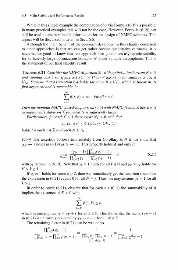
6.5 Main Stability and Performance Results 127
While in this simple example the computation of α via Formula (6.19) is possible,in many practical examples this will not be the case. However, Formula (6.19) canstill be used to obtain valuable information for the design of NMPC schemes. Thisaspect will be discussed in detail in Sect. 6.6.
Although the main benefit of the approach developed in this chapter comparedto other approaches is that we can get rather precise quantitative estimates, it isnevertheless good to know that our approach also guarantees asymptotic stabilityfor sufficiently large optimization horizons N under suitable assumptions. This isthe statement of our final stability result.
Theorem 6.21 Consider the NMPC Algorithm 3.1 with optimization horizon N ∈ N
and running cost � satisfying α3(|x|x∗) ≤ �∗(x) ≤ α4(|x|x∗) for suitable α3, α4 ∈K∞. Suppose that Assumption 6.4 holds for some β ∈ K L0 which is linear in itsfirst argument and is summable, i.e.,
∞∑
k=0
β(r, k) < ∞ for all r > 0.
Then the nominal NMPC closed-loop system (3.5) with NMPC-feedback law μN isasymptotically stable on X provided N is sufficiently large.
Furthermore, for each C > 1 there exists NC > 0 such that
J∞(x,μN) ≤ CVN(x) ≤ CV∞(x)
holds for each x ∈ X and each N ≥ NC .
Proof The assertion follows immediately from Corollary 6.19 if we show thatαN → 1 holds in (6.19) as N → ∞. This property holds if and only if
limN→∞
(γN − 1)∏N
k=2(γk − 1)∏N
k=2 γk −∏Nk=2(γk − 1)
= 0 (6.21)
with γk defined in (6.19). Note that γk ≥ 1 holds for all k ∈ N and γk′ ≥ γk holds fork′ > k ≥ 1.
If γk = 1 holds for some k ≥ 2, then we immediately get the assertion since thenthe expression in (6.21) equals 0 for all N ≥ j . Thus, we may assume γk > 1 for allk ≥ 2.
In order to prove (6.21), observe that for each ε ∈ (0,1) the summability of β
implies the existence of K > 0 with∞∑
k=K
β(1, k) ≤ ε,
which in turn implies γk ≤ γK + ε for all k ∈ N. This shows that the factor (γN − 1)
in (6.21) is uniformly bounded by γK + ε − 1 for all N ∈ N.The remaining factor in (6.21) can be written as
∏Nk=2(γk − 1)
∏Nk=2 γk −∏N
k=2(γk − 1)= 1
∏Nk=2 γk−∏N
k=2(γk−1)∏N
k=2(γk−1)
= 1∏N
k=2γk
γk−1 − 1.

128 6 Stability and Suboptimality Without Stabilizing Constraints
Now the estimates γK ≤ γk ≤ γK + ε for all k ≥ K imply for N > K
N∏
k=2
γk
γk − 1≥
K∏
k=2
γk
γk − 1
(γK
γK + ε − 1
)N−K
→ ∞
as N → ∞, since ε < 1 and thus γK + ε − 1 < γK . Thus,
limN→∞
∏Nk=2(γk − 1)
∏Nk=2 γk −∏N
k=2(γk − 1)= lim
N→∞1
∏Nk=2
γk
γk−1 − 1= 0,
which shows the claim. �
This theorem justifies what is often done in practice: we set up an NMPC schemeusing a reasonable running cost � and increase N until the closed-loop system be-comes stable. While this procedure may work in many applications, it is certainlynot the most sophisticated way to proceed and a clever design of � may signifi-cantly improve the performance. Examples in which this is the case can be found inSect. 6.6.
Remark 6.22 Recall from Sect. 6.1 that throughout this chapter we use our standingassumption that X is viable. This property is needed in order to ensure recursivefeasibility of X, cf. the discussion after Theorem 3.5. Approaches which allow usto relax these assumptions are discussed in Sects. 8.1–8.3, cf. also the discussion inSect. 8.4(iv).
Theorem 6.18 and Corollary 6.19 give a sufficient condition for asymptotic sta-bility for the nominal NMPC closed-loop system (3.5) in terms of the value α. Moreprecisely, if α from (6.14) or αN from (6.19), respectively, is positive, then we canconclude asymptotic stability whenever Assumption 6.4 is satisfied for the optimiza-tion problem (OCPN) in Algorithm 3.1.
The following theorem shows that for β ∈ K L0 satisfying (6.6)—which impliesα = αN if β is linear in its first argument—this condition is tight for the class ofsystems satisfying Assumption 6.4 in the following sense: if α from (6.14) is nega-tive, then there exists a control system (2.1) and a running cost � such that Assump-tion 6.4 holds but the nominal NMPC closed-loop system (3.5) is not asymptoticallystable.
Theorem 6.23 Consider β ∈ K L0 satisfying (6.6), let N ≥ 1 and assume that theoptimization problem (6.14) has an optimal value α < 0.
Then there exists a control system (2.1) and a running cost � satisfying Assump-tion 6.4 and α3(|x|x∗) ≤ �∗(x) ≤ α4(|x|x∗) for suitable α3, α4 ∈ K∞, such that thenominal NMPC closed-loop system (3.5) is not asymptotically stable.
Proof We first show that α < 0 in (6.14) implies the following property:

6.5 Main Stability and Performance Results 129
there exists λ0, . . . , λN−1, ν > 0 satisfying
(6.11) with strict inequalities, (6.12) and (6.22)N−1∑
n=0
λn − ν < 0.
In order to prove (6.22) we use that α < 0 in (6.14) yields the existence of λ0 > 0,λ1, . . . , λN−1, ν ≥ 0 satisfying (6.11), (6.12) and
N−1∑
n=0
λn − ν < 0. (6.23)
These properties imply λ1 > 0, . . . , λN−1 > 0 and ν > 0: the inequality ν > 0immediately follows from (6.23) and λk ≥ 0. Assuming λk = 0 for some k ∈{1, . . . ,N − 1}, the respective inequality from (6.11) together with BN−k(0) = 0implies λk+1 = · · · = λN−1 = 0. Thus, in particular λN−1 = 0, which using (6.12)for j = N − 2 implies ν ≤∑N−3
n=0 λn+1, contradicting (6.23).Now we pick an arbitrary ε > 0 and set
λ0 := λ0, . . . , λN−2 := λN−2, λN−1 := λN−1 − ε,
and
ν := min
{
ν,
N−2∑
n=0
λn+1 + B2(λN−1)
}
.
We claim that for these values (6.22) holds for all sufficiently small ε > 0. In orderto see this, first one easily checks that (6.11) and (6.12) hold. Furthermore, sinceλN−1 < λN−1 appears on the left hand side but not on the right hand side of eachinequality in (6.11), it follows that the inequalities in (6.11) are indeed strict. Fur-thermore, for ε > 0 sufficiently small the inequality λN−1 > 0 holds. In order tocomplete the proof of (6.22) it remains to show that for ε > 0 sufficiently small theinequality ν > 0 and the inequality in the last line of (6.22) holds.
To this end, we use that the second term in the “min” is exactly (6.12) for j =N − 2. Thus, by continuity of B2 the value ν converges to ν > 0 as ε → 0. Hence,for ε > 0 sufficiently small ν > 0 implies ν > 0 and (6.23) implies the inequality inthe last line of (6.22), which completes the proof of (6.22).
Now we construct a control system (2.1) on the state space
X = {(q,p) ∈ R
2∣∣ q ∈ {0} ∪ {
2−k∣∣ k ∈ N0
},p ∈ {(−N + 1)q, . . . ,Nq
}}.
For the control values U = {−1,0,1} we define the dynamics
f((1,p),−1
) = (1,max{−N + 1,p − 1}), p ∈ {(−N + 1)q, . . . ,Nq
},
f((1,p),0
) = (1/2,p/2), p ∈ {(−N + 1)q, . . . ,Nq},
f((1,p),1
) = (1,min{N,p + 1}), p ∈ {(−N + 1)q, . . . ,Nq
},
f((q,p),u
) = (q/2,p/2), (q,p) ∈ X, q ≤ 1/2, u ∈ U

130 6 Stability and Suboptimality Without Stabilizing Constraints
for which x∗ = (0,0) is an equilibrium for all u ∈ U . On X we use the metricinduced by the usual Euclidean norm ‖(q,p)‖ =√
q2 + p2 implying ‖x‖x∗ = ‖x‖.We do not impose any constraints, i.e., we set X = X and U(x) = U for all x ∈ X.
Using the values λ1, . . . , λN−1 and ν from (6.22) we define the running cost � in(OCPN) as
�((1,p),1
) = λp, p ∈ {0,N − 1},�((1,p),1
) = ν, p /∈ {0,N − 1},�((1,p),−1
) = �((1,−p + 1),1
),
�((1,p),0
) = β(min
{�((1,p),1
), �((1,p),−1
)},0),
�((
2−k,p), u) = β
(min
{�((
1,2kp),1), �((
1,2kp),−1
)}, k), k ≥ 1, u ∈ U.
We first verify that f and � satisfy the stated assumptions.The running cost � satisfies the inequalities from the assumption for α′
3(r) =infx∈X,‖x‖≥r �∗(x) and α′
4(r) = supx∈X,‖x‖≤r �∗(x). Due to the discrete nature of thestate space α′
3 and α′4 are discontinuous but they are easily under- and overbounded
by continuous K∞ functions α3 and α4, respectively, for which the assumed in-equalities α3(|x|x∗) ≤ �∗(x) ≤ α4(|x|x∗) hold.
In order to see that Assumption 6.4 is satisfied for the given β , first observe thatAssumption 6.4 for n = 0 implies β(r,0) ≥ r . From this inequality and the definitionof � we obtain
�((1,p),0
)≥ min{�((1,p),1
), �((1,p),−1
)}
and thus
�∗((1,p))= min
{�((1,p),1
), �((1,p),−1
)}.
Furthermore, for k ≥ 1 we see that �((2−k,p),u) is independent of u, which yields
�∗((2−k,p))= �
((2−k,p
),0).
Now for ux ≡ 0 and initial value x = (q,p) ∈ X with q = 2−k0 the trajectory be-comes
xux (k, x) = (2−k−k0 ,2−kp
).
Thus, by construction of � and (6.6) we obtain
�(xux
(k, x), ux(k))= β
(min
{�((
1,2k0p),1), �((
1,2k0p),−1
)}, k + k0
)
= β(�∗(1,2k0p
), k + k0
)
≤ β(β(�∗(1,2k0p
), k0
), k)= β
(�((
2−k0 ,p),0), k)
= β(�∗((2−k0 ,p
)), k)= β
(�∗(x), k
),
which yields Assumption 6.4.Now we prove the existence of a closed-loop trajectory which does not converge
to x∗, which shows that asymptotic stability does not hold. To this end we abbre-viate � = ∑N−1
n=0 λn (note that (6.22) implies ν > �) and investigate the valuesJN((1,0), u) for different choices of u:

6.5 Main Stability and Performance Results 131
Case 1 u(0) = 0. In this case, regardless of the values u(n), n ≥ 1, we obtainx(n,u) = (2−n,0) and thus
JN
((1,0), u
)=N−1∑
n=0
β(min
{�((1,0),1
), �((1,0),−1
)}, n)
= BN
(min
{�((1,0),1
), �((1,0),−1
)})= BN
(min{λ0, λ1}
).
In case that the minimum is attained in λ0, by the (strict) Inequality (6.11) for k = 0we obtain JN((1,0), u) > �. If the minimum is attained in λ1 then by (6.12) forj = 0 and (6.22) we obtain JN((1,0), u) ≥ ν > �. Thus, in both cases the inequalityJN((1,0), u) > � holds.
Case 2 u(n) = −1, n = 0, . . . ,N − 2. This choice yields x(n,u) = (1,−n) forn = 0, . . . ,N − 1 and thus
JN
((1,0), u
)=N−2∑
n=0
λn+1 + �((
1,−(N − 1)),−1
)≥ �((
1,−(N − 1)),−1
)
= �((1,N),1
)= ν > �.
Case 3 u(n) = −1, n = 0, . . . , k − 1, and u(k) = 1 for a k ∈ {1, . . . ,N − 2}. In thiscase we obtain x(n,u) = (1,−n) for n = 0, . . . , k implying
JN
((1,0), u
)=k−1∑
n=0
λn+1 + �((1,−k),1
)≥ �((1,−k),1
)= ν > �.
Case 4 u(n) = −1, n = 0, . . . , k − 1, and u(k) = 0 for a k ∈ {1, . . . ,N − 2}.This control sequence yields x(n,u) = (1,−n) for n = 0, . . . , k while for n =k + 1, . . . ,N − 1 we get x(n,u) = (2−(n−k),−2−(n−k)k). Thus
JN
((1,0), u
)=k−1∑
n=0
λn+1 +N−1∑
n=k
β(min
{�((1,−k),1
), �((1,−k),−1
)}, n − k
)
=k−1∑
n=0
λn+1 + BN−k(λk+1) ≥ ν > �,
where we have used (6.12) for j = k in the second last inequality.
Case 5 u(n) = 1, n = 0, . . . ,N − 1. This yields x(n,u) = (1, n) and thus
JN
((1,0), u
)=N−1∑
n=0
λn = �.
Summarizing, we obtain that any optimal control ux for x = (1,0) must satisfy
ux(0) = 1 because for u(0) = 1 we can realize a value ≤ � while for u(0) �= 1 we

132 6 Stability and Suboptimality Without Stabilizing Constraints
inevitably obtain a value > �. Consequently, the NMPC-feedback law μN(x) =u
x(0) will steer the system from x = (1,0) to x+ := (1,1).Now we use that by construction f and � have the symmetry properties
f((q,p),u
)− (0,p) = −f((q,−p + q),−u
)+ (0,−p + q),
�((q,p),u
)= �((q,−p + q),−u
)
for all (q,p) ∈ X, which implies J ((q,p),u) = J ((q,−p + q),−u). Observe thatx+ = (1,1) is exactly the symmetric counterpart of x = (1,0). Thus, any optimalcontrol u
x+ for x+ must satisfy ux+(n) = −u
x(n) for some optimal control ux for
initial value x. Hence, we obtain ux+(0) = −1, which means that the NMPC feed-
back μN(x+) = ux+(0) steers x+ back to x. Thus, under the NMPC-feedback law
we obtain the closed-loop trajectory (x, x+, x, x+, . . .), which clearly does not con-verge to x∗ = (0,0). This shows that the closed-loop system is not asymptoticallystable. �
Remark 6.24 If we weaken the assumptions of Theorem 6.23 to α = 0 instead ofα < 0, then the inequalities in (6.22) will not be strict. Under this weaker assump-tion, in Cases 1–4 in the proof of Theorem 6.23 we get JN((1,0), u) ≥ � insteadof JN((1,0), u) > �. This means that the control sequence u(n) ≡ 1 from Case 5 isstill optimal but it is no longer the unique optimal control sequence. Consequently,the value of μN((1,0)) depends on the optimization algorithm. The algorithm mayselect μN((1,0)) = 1—leading to a closed-loop system which is not asymptoticallystable—or it may select a control value which yields asymptotic stability. Thus, in-stability may occur for α = 0 but it does not necessarily need to occur.
All results developed so far in this chapter remain valid for the time varyingcase when the Controllability Assumption 6.4 holds uniformly in time, i.e., if thefollowing assumption holds.
Assumption 6.25 Consider the optimal control problem (OCPnN). We assume that
the system is uniformly asymptotically controllable with respect to � with rate β ∈K L0, i.e., for each x ∈ X, each N ∈ N and each n0 ∈ N0 there exists an admissiblecontrol sequence ux ∈ U
N(x) satisfying
�(n0 + n,xux (n, x),ux(n)
)≤ β(�∗(n0, x), n
)
for all n ∈ {0, . . . ,N − 1}.
Under this assumption, all results in this chapter carry over to the time-dependentsetting when we replace λk and ν in Proposition 6.12 by
λk = �(n0 + k, xu(k, x), u(k)
)and ν = VN
(n0 + 1, xu(1, x)
).
Proceeding this way, one easily sees that all results remain valid.

6.6 Design of Good Running Costs � 133
Fig. 6.1 Suboptimality regions for different optimization horizons N depending on C and σ in(6.3) for α = 0 (left) and α = 0.5 (right)
6.6 Design of Good Running Costs �
In this section we illustrate by means of several examples how our theoretical find-ings and in particular Theorem 6.14 in conjunction with Proposition 6.17 can beused in order to identify and design running costs � such that the NMPC feedbacklaw μN exhibits stability and good performance with small optimization horizonsN . To this end we first visualize Formula (6.19) for different β ∈ K L0, starting withthe case of exponential controllability (6.3). Note that in this case (6.6) and thus(6.20) always holds.
Given a desired suboptimality level α ≥ 0, we use Formula (6.19) in order todetermine the regions in the (σ,C)-plane for which αN ≥ α holds for differentoptimization horizons N . Figure 6.1 shows the resulting regions for α = 0 (i.e.,“plain” stability) and α = 0.5.
Looking at Fig. 6.1 one sees that the parameters C and σ play a very differ-ent role. While for both parameters the necessary optimization horizon N becomesthe smaller the smaller these parameters are, small overshoot C (i.e., values of C
close to 1) have a much stronger effect than small decay rates σ (i.e., values of σ
close to 0). Indeed, Fig. 6.1(left) shows that for sufficiently small C we can alwaysachieve stability for N = 2 while for C ≥ 8 even values of σ very close to 0 willnot yield stability for N ≤ 16. For the required higher suboptimality level α ≥ 0.5,Fig. 6.1(right) indicates a qualitatively similar behavior.
For finite time control, i.e., controllability with K L0-functions satisfying (6.4),the situation is very similar. For instance, consider functions of the form β(r,0) =c0r , β(r,1) = c1r , c0 ≥ c1, and β(r, n) = 0 for n ≥ 2, i.e., n0 = 2. This functionagain satisfies (6.6), hence (6.20) holds. For this β , Fig. 6.2 shows the analogousgraphs as in Fig. 6.1.
One immediately sees that the qualitative behavior depicted in Fig. 6.2 is verysimilar to the analogous graphs in Fig. 6.1: again, reducing the overshoot c0 we can

134 6 Stability and Suboptimality Without Stabilizing Constraints
Fig. 6.2 Suboptimality regions for different optimization horizons N depending on c0 and c1/c0in (6.4) with n0 = 2 for α = 0 (left) and α = 0.5 (right)
always achieve stability with N = 2 regardless of the ratio c1/c0 while reducing c1
and keeping c0 fixed, in general we need N > 2 in order to guarantee stability.Finally, in Fig. 6.3 we compare the effect of the overshoot c0 and the time n0
in (6.4) by using β(r,0) = c0r , β(r, n) = c0r/2 for n = 1, . . . , n0 and β(r, n) = 0for n ≥ n0. Again, it turns out that the time n0 needed to control the system to x∗is less important than the overshoot: for all times n0 ≥ 1 we can always achievestability for c0 sufficiently close to 1 while for fixed c0 this can in general not beachieved even for n0 = 1, i.e., for controllability in one step. Note that for c0 < 2this function β does not satisfy (6.6), thus for these values of c0 Formula (6.19)only provides a lower bound for α, cf. (6.18). Consequently, for c0 < 2 the regionsdepicted in Fig. 6.3 may underestimate the true regions. Still, for all n0 the lowerbounds obtained from (6.18) ensure both asymptotic stability and the desired per-formance bound α ≥ 0.5 for N = 2 whenever c0 is sufficiently close to 1.
Together, these examples lead to a conclusion which is as intuitive as simple:an NMPC controller without stabilizing terminal constraints will yield stability andgood performance for small horizons N if � can be chosen such that Assumption 6.4is satisfied with a β ∈ K L0 with small overshoot. Thus, the criterion “small over-shoot” can be used as a design guideline for selecting a good running cost �.
For some systems, it is possible to rigorously compute β in Assumption 6.4,which leads to a precise determination of, e.g., C and σ in (6.3). Examples wherethis is possible also include infinite-dimensional systems, like the linear wave equa-tion or certain classes of semilinear parabolic equations, cf. [3]. However, moreoften than not precise estimates for β cannot be obtained due to the complexity ofthe dynamics. Still, using heuristic arguments it may be possible to determine run-ning costs � for which the overshoot is reduced. In the remainder of this section wewill illustrate this procedure for two examples.

6.6 Design of Good Running Costs � 135
Fig. 6.3 Suboptimality regions for different optimization horizons N depending on c0 and n0 in(6.4) with cn = c0/2 for n = 1, . . . , n0 − 1 for α = 0 (left) and α = 0.5 (right)
Example 6.26 We consider Example 2.3, i.e.,
f (x,u) :=(
x+1
x+2
)=(
sin(ϑ(x) + u)
cos(ϑ(x) + u)/2
)
with
ϑ(x) ={
arccos 2x2, x1 ≥ 0,
2π − arccos 2x2, x1 < 0
using the control values U = [0,0.2], i.e., the car can only move clockwise on theellipse
X ={x ∈ R
2∣∣∣∣
∥∥∥∥
(x12x2
)∥∥∥∥= 1
}.
As in illustrated in Fig. 6.4, we want to stabilize the system at the equilibrium x∗ =(0,−1/2)� starting from the initial value x0 = (0,1/2)�.
Interpreting X as a subset of R2, we can try to achieve this goal by using NMPC
without terminal constraints with the running cost
�(x,u) = ‖x − x∗‖2 + u2. (6.24)
As the simulations in Fig. 6.5 show, asymptotic stability of x∗ = (0,−1/2) isachieved for N = 11 but not for N = 10.
The reason for the closed loop not being asymptotically stable for N = 10 (and,in fact, for all N ≤ 10) is the overshoot in the running cost � when moving alongthe ellipse; see Fig. 6.6.
The fact that this overshoot of � appears along the NMPC closed-loop trajec-tory does in general not imply that the overshoot is present for all possible controlsequences u controlling the system to x∗. However, in this example a look at thegeometry reveals that for � from (6.24) the overshoot is in fact not avoidable: no

136 6 Stability and Suboptimality Without Stabilizing Constraints
Fig. 6.4 Illustration of thestabilization problem
matter how we control the system to x∗, before we can eventually reduce � to 0, weneed to increase � when moving along the ellipse around the curve. Thus, looselyspeaking, the loss of asymptotic stability for N ≤ 10 is caused by the fact that theoptimizer does not “see” that in the long run it is beneficial to move around the curveand thus stays at the initial value x0 for all future times.
Looking closer at the geometry of the example, one easily sees that the overshootis entirely due to the x1-component of the solution: while x2 converges monotoni-cally to the desired position x∗2 = −0.5, x1 first needs to move from 0 to 1 beforewe can eventually control it to x∗1 = 0, again. From this observation it follows thatthe overshoot in � can be avoided by putting more weight on the x2-component.Indeed, if we replace �(x,u) = ‖x − x∗‖2 + u2 = (x1 − x∗1)
2 + (x2 − x∗2)2 + u2
from (6.24) by
�(x,u) = (x1 − x∗1)2 + 5(x2 − x∗2)
2 + u2, (6.25)
then we obtain asymptotic stability even for N = 2, cf. Fig. 6.7.Figure 6.8 shows the running cost along the closed-loop trajectory for this ex-
ample. The figure clearly shows that the overshoot has been removed completely,which explains why the NMPC closed loop is stable for N = 2.
We would like to emphasize that for removing the overshoot we did not use anyquantitative information, i.e., we did not attempt to estimate the function β in As-sumption 6.4. For selecting a good cost function � it was sufficient to observe thatputting a larger weight on x2 will reduce the overshoot. On the basis of this obser-vation, the fact that the weight “5” used in (6.25) is sufficient to achieve asymptoticstability with N = 2 was then determined by a simple try-and-error procedure usingnumerical simulations.
Example 6.27 As a second example we consider the infinite-dimensional PDEmodels introduced in Example 2.12. We first consider the system with distributedcontrol, i.e.,
yt (t, x) = θyxx(t, x) − yx(t, x) + ρ(y(t, x) − y(t, x)3)+ u(t, x) (6.26)
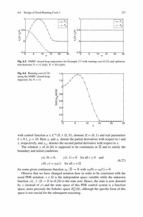
6.6 Design of Good Running Costs � 137
Fig. 6.5 NMPC closed-loop trajectories for Example 2.3 with running cost (6.24) and optimiza-tion horizons N = 11 (left), N = 10 (right)
Fig. 6.6 Running cost (6.24)along the NMPC closed-looptrajectory for N = 11
with control function u ∈ L∞(R × �,R), domain � = (0,1) and real parametersθ = 0.1, ρ = 10. Here yt and yx denote the partial derivatives with respect to t andx, respectively, and yxx denotes the second partial derivative with respect to x.
The solution y of (6.26) is supposed to be continuous in � and to satisfy theboundary and initial conditions
y(t,0) = 0, y(t,1) = 0 for all t ≥ 0 and(6.27)
y(0, x) = y0(x) for all x ∈ �
for some given continuous function y0 : � → R with y0(0) = y0(1) = 0.Observe that we have changed notation here in order to be consistent with the
usual PDE notation: x ∈ � is the independent space variable while the unknownfunction y(t, ·) : � → R in (6.26) is the state now. Hence, the state is now denotedby y (instead of x) and the state space of this PDE control system is a functionspace, more precisely the Sobolev space H 1
0 (�), although the specific form of thisspace is not crucial for the subsequent reasoning.

138 6 Stability and Suboptimality Without Stabilizing Constraints
Fig. 6.7 NMPC closed-looptrajectories for Example 2.3with running cost (6.25) andoptimization horizon N = 2
Fig. 6.8 Running cost (6.25)along the NMPC closed loopfor N = 2
Figure 6.9 shows the solution of the uncontrolled system (6.26), (6.27), i.e., withu ≡ 0. For growing t the solution approaches an asymptotically stable steady statey∗∗ �= 0. The figure (as well as all other figures in this section) was computed nu-merically using a finite difference scheme with 50 equidistant nodes on (0,1) (finerresolutions did not yield significantly different results) and initial value y0 withy0(0) = y0(1) = 0, y0|[0.02,0.3] ≡ −0.1, y0|[0.32,0.98] ≡ 0.1 and linear interpolationin between.
By symmetry of (6.26) the function −y∗∗ must be an asymptotically stable steadystate, too. Furthermore, from (6.26) it is obvious that y∗ ≡ 0 is another steady state,which is, however, unstable. Our goal is now to use NMPC in order to stabilize theunstable equilibrium y∗ ≡ 0.
To this end we consider the sampled data system corresponding to (6.26) withsampling period T = 0.025. In order to obtain a more intuitive notation for thesolution of the sampled data system, instead of introducing the abstract variable z

6.6 Design of Good Running Costs � 139
Fig. 6.9 Solution y(t, x) of(6.26), (6.27) with u ≡ 0
as in Example 2.12 here we denote the state of the sampled data system at the nthsampling instant, i.e., at time nT by y(n, ·). For penalizing the distance of the statey(n, ·) to y∗ ≡ 0 a popular choice in the literature is the L2 functional
�(y(n, ·), u(n, ·))= ∥∥y(n, ·)∥∥2
L2(�)+ λ
∥∥u(n, ·)∥∥2L2(�)
, (6.28)
which penalizes the mean squared distance from y(n, ·) to y∗ ≡ 0 and the controleffort with weighting parameter λ > 0. Here we choose λ = 0.1.
Another possible choice of measuring the distance to y∗ ≡ 0 is obtained by usingthe H 1 norm
∥∥y(n, ·)∥∥
H 1(�)= ∥∥y(n, ·)∥∥2
L2(�)+ ∥∥yx(n, ·)∥∥2
L2(�).
This leads us to define
�(y(n, ·), u(n, ·))= ∥∥y(n, ·)∥∥2
L2(�)+ ∥∥yx(n, ·)∥∥2
L2(�)
+ λ∥∥u(n, ·)∥∥2
L2(�), (6.29)
which in addition to the L2 distance and the control effort as in (6.28) also penal-izes the mean squared distance from yx(n, ·) to y∗,x ≡ 0. Figs. 6.10 and 6.11 showthe respective NMPC closed-loop solutions with optimization horizons N = 3 andN = 11.
Figure 6.10 indicates that for N = 3 the NMPC scheme with � from (6.28) doesnot stabilize the system at y∗ ≡ 0, while for � from (6.29) it does. For (6.28) we needan optimization horizon of at least N = 11 in order to obtain a stable closed-loopsolution, cf. Fig. 6.11. For � from (6.29) the right images in Figs. 6.10 and 6.11 showthat enlarging the horizon does not improve the closed-loop behavior any further.
Using our theoretical results we can explain why � from (6.29) performs muchbetter for small horizons N . For this example our controllability condition Assump-tion 6.4 reads
�(y(n, ·), u(n, ·))≤ Cσn�∗(y(0, ·)). (6.30)

140 6 Stability and Suboptimality Without Stabilizing Constraints
Fig. 6.10 NMPC closed loop for (6.26) with N = 3 and � from (6.28) (left) and (6.29) (right)
Fig. 6.11 NMPC closed loop for (6.26) with N = 11 and � from (6.28) (left) and (6.29) (right)
For � from (6.28) this becomes∥∥y(n, ·)∥∥2
L2(�)+ λ
∥∥u(n, ·)∥∥2L2(�)
≤ Cσn∥∥y(0, ·)∥∥2
L2(�). (6.31)
Now in order to control the system to y∗ ≡ 0, in (6.26) the control needs to com-pensate for yx and ρ(y(t, x) − y(t, x)3), i.e., any control steering y(n, ·) to 0 mustsatisfy
∥∥u(n, ·)∥∥2L2(�)
≈ ∥∥yx(n, ·)∥∥2L2(�)
+ ∥∥ρ(y(n, ·) − y(n, ·)3)∥∥2
L2(�). (6.32)
Inserting this approximate equality into (6.31) implies—regardless of the value ofσ—that the overshoot bound C in (6.31) is large if ‖yx(n, ·)‖2
L2(�)� ‖y(0, ·)‖2
L2(�)
holds, which is the case in our example.For � from (6.29) Inequality (6.30) becomes
∥∥y(n, ·)∥∥2L2(�)
+ ∥∥yx(n, ·)∥∥2L2(�)
+ λ∥∥u(n, ·)∥∥2
L2(�)
≤ Cσn(∥∥y(0, ·)∥∥2
L2(�)+ ∥∥yx(0, ·)∥∥2
L2(�)
). (6.33)

6.6 Design of Good Running Costs � 141
Fig. 6.12 NMPC closed loop for (6.34) with N = 15 and � from (6.28) (left) and (6.29) (right)
Due to the fact that ‖yx(0, ·)‖2L2(�)
� ‖y(0, ·)‖2L2(�)
holds in our example, insertingthe approximate equation (6.32) into (6.33) does not imply large C, which explainsthe considerable better performance for � from (6.29).
The fact that the H 1-norm penalizes the distance to y∗ ≡ 0 in a “stronger” waythan the L2-norm may lead to the conjecture that the better performance for thisnorm is intuitive. Our second example shows that this is not the case. This exampleis similar to equations (6.26), (6.27), except that the distributed control is changedto Dirichlet boundary control. Thus, (6.26) becomes
yt (t, x) = θyxx(t, x) − yx(t, x) + ρ(y(t, x) − y(t, x)3), (6.34)
again with θ = 0.1 and ρ = 10, and (6.27) changes to
y(t,0) = u0(t), y(t,1) = u1(t) for all t ≥ 0,
y(0, x) = y0(x) for all x ∈ �
with u0, u1 ∈ L∞(R,R). The cost functions (6.28) and (6.29) change to
�(y(n, ·), u(n, ·))= ∥∥y(n, ·)∥∥2
L2(�)+ λ
(u0(n)2 + u1(n)2) (6.35)
and
�(y(n, ·), u(n, ·))= ∥∥y(n, ·)∥∥2
L2(�)+ ∥∥yx(n, ·)∥∥2
L2(�)
+ λ(u0(n)2 + u1(n)2), (6.36)
respectively, again with λ = 0.1.Due to the more limited possibilities to control the equation the problem obvi-
ously becomes more difficult, hence we expect to need larger optimization horizonsfor stability of the NMPC closed loop. However, what is surprising at first glance isthat � from (6.35) stabilizes the system for smaller horizons than � from (6.36), asthe numerical results in Fig. 6.12 confirm.
A closer look at the dynamics reveals that we can again explain this behavior withour theoretical results. In fact, steering the chosen initial solution to y∗ = 0 requiresu1 to be such that a rather large gradient appears close to x = 1. Thus, during the

142 6 Stability and Suboptimality Without Stabilizing Constraints
transient phase ‖yx(n, ·)‖2L2(�)
becomes large, which in turn causes � from (6.36)to become large and thus causes a large overshoot bound C in (6.30). In � from(6.35), on the other hand, these large gradients are not “visible”, which is why theovershoot in (6.30) is smaller and thus allows for stabilization with smaller N .
6.7 Semiglobal and Practical Asymptotic Stability
We have seen in Theorem 6.21 that linearity of β in Assumption 6.4 guaranteesthat for sufficiently large optimization horizon N the nominal NMPC closed-loopsystem (3.5) will be asymptotically stable on the whole set X. Even though theexamples in the last section show that this condition can be fulfilled, it is easy tocome up with examples in which this property is not satisfied or at least difficultor almost impossible to check. In this section we show that also in this case onecan guarantee that NMPC without stabilizing terminal constraints has reasonablestability properties. However, to this end we have to weaken the stability notionaccording to the following definition.
Definition 6.28 Consider the NMPC Algorithm 3.1 and the resulting nominalclosed-loop system (3.5) with feedback law μN and solutions xμN
(k, x).
(i) We call the closed-loop system (3.5) semiglobally asymptotically stable withrespect to the optimization horizon N if there exists β ∈ K L such that the fol-lowing property holds: for each � > 0 there exists N� ∈ N such that for allN ≥ N� and all x ∈ X with |x|x∗ ≤ � the inequality
∣∣xμN(k, x)
∣∣x∗ ≤ β
(|x|x∗, k)
holds for all k ∈ N0.(ii) We call the closed-loop system (3.5) semiglobally practically asymptotically
stable with respect to the optimization horizon N if there exists β ∈ K L suchthat the following property holds: for each δ > 0 and � > δ there exists Nδ,� ∈N such that for all N ≥ Nδ,� and all x ∈ X with |x|x∗ ≤ � the inequality
∣∣xμN
(k, x)∣∣x∗ ≤ max
{β(|x|x∗, k
), δ}
holds for all k ∈ N0.
Semiglobal asymptotic stability relaxes the asymptotic stability condition by re-quiring asymptotic stability only for the set of initial values x ∈ X with |x|x∗ ≤ �.Although � can be chosen arbitrarily large by suitably adjusting the optimizationhorizon N , for each finite N it will in general be a finite value.
Semiglobal practical asymptotic stability additionally relaxes the requirementthat the solution exactly tends to the equilibrium x∗ by only requiring that the solu-tion behaves like an asymptotically stable solution until it reaches a δ-neighborhoodof x∗. Similar to the value of �, the size δ of this neighborhood can be arbitrar-ily tuned by adjusting the optimization horizon N , but for each finite N it will ingeneral be a positive value.
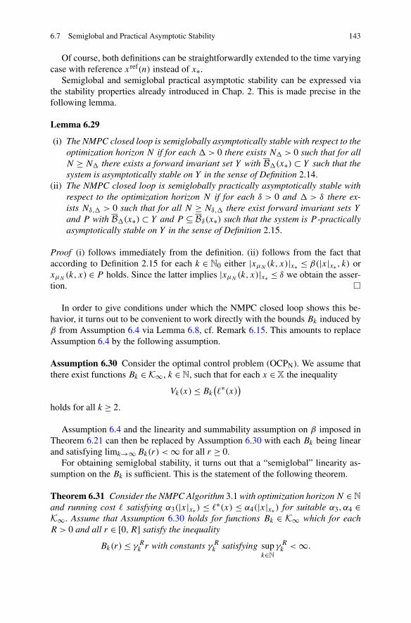
6.7 Semiglobal and Practical Asymptotic Stability 143
Of course, both definitions can be straightforwardly extended to the time varyingcase with reference xref(n) instead of x∗.
Semiglobal and semiglobal practical asymptotic stability can be expressed viathe stability properties already introduced in Chap. 2. This is made precise in thefollowing lemma.
Lemma 6.29
(i) The NMPC closed loop is semiglobally asymptotically stable with respect to theoptimization horizon N if for each � > 0 there exists N� > 0 such that for allN ≥ N� there exists a forward invariant set Y with B�(x∗) ⊂ Y such that thesystem is asymptotically stable on Y in the sense of Definition 2.14.
(ii) The NMPC closed loop is semiglobally practically asymptotically stable withrespect to the optimization horizon N if for each δ > 0 and � > δ there ex-ists Nδ,� > 0 such that for all N ≥ Nδ,� there exist forward invariant sets Y
and P with B�(x∗) ⊂ Y and P ⊆ Bδ(x∗) such that the system is P -practicallyasymptotically stable on Y in the sense of Definition 2.15.
Proof (i) follows immediately from the definition. (ii) follows from the fact thataccording to Definition 2.15 for each k ∈ N0 either |xμN
(k, x)|x∗ ≤ β(|x|x∗, k) orxμN
(k, x) ∈ P holds. Since the latter implies |xμN(k, x)|x∗ ≤ δ we obtain the asser-
tion. �
In order to give conditions under which the NMPC closed loop shows this be-havior, it turns out to be convenient to work directly with the bounds Bk induced byβ from Assumption 6.4 via Lemma 6.8, cf. Remark 6.15. This amounts to replaceAssumption 6.4 by the following assumption.
Assumption 6.30 Consider the optimal control problem (OCPN). We assume thatthere exist functions Bk ∈ K∞, k ∈ N, such that for each x ∈ X the inequality
Vk(x) ≤ Bk
(�∗(x)
)
holds for all k ≥ 2.
Assumption 6.4 and the linearity and summability assumption on β imposed inTheorem 6.21 can then be replaced by Assumption 6.30 with each Bk being linearand satisfying limk→∞ Bk(r) < ∞ for all r ≥ 0.
For obtaining semiglobal stability, it turns out that a “semiglobal” linearity as-sumption on the Bk is sufficient. This is the statement of the following theorem.
Theorem 6.31 Consider the NMPC Algorithm 3.1 with optimization horizon N ∈ N
and running cost � satisfying α3(|x|x∗) ≤ �∗(x) ≤ α4(|x|x∗) for suitable α3, α4 ∈K∞. Assume that Assumption 6.30 holds for functions Bk ∈ K∞ which for eachR > 0 and all r ∈ [0,R] satisfy the inequality
Bk(r) ≤ γ Rk r with constants γ R
k satisfying supk∈N
γ Rk < ∞.

144 6 Stability and Suboptimality Without Stabilizing Constraints
Then the nominal NMPC closed-loop system (3.5) with NMPC feedback law μN issemiglobally asymptotically stable on X with respect to the optimization horizon N .
Furthermore, for each C > 1 and each � > 0 there exists NC,� > 0 such that
J∞(x,μN) ≤ CVN(x) ≤ CV∞(x)
holds for each x ∈ B�(x∗) ∩ X and each N ≥ NC,�.
Proof We first show the existence of α ∈ K∞ such that the inequality Bk(r) ≤ α(r)
holds for all r ≥ 0 and all k ∈ N. To this end, we define γ R∞ := supk∈Nγ Rk for each
R > 0. Then the inequality Bk(r) ≤ γ R∞r holds for all k ∈ N and all r ∈ [0,R]. Nowfor R = 1,2, . . . we inductively define γ 1 = γ 1∞ and
γ R+1 = max{γ R,γ R+1∞
}.
This definition implies γ R+1 ≥ γ R and Bk(r) ≤ γ Rr for all r ∈ [0,R], R ∈ N.Setting
α(r) := (R − r)γ Rr + (r − R + 1)γ R+1r, r ∈ [R − 1,R], R ∈ N
we obtain a continuous, strictly increasing and unbounded function with α(0) = 0,hence α ∈ K∞. For r ∈ [R − 1,R] and R ∈ N we obtain
Bk(r) ≤ γ Rr = (R − r)γ Rr + (r − R + 1)γ Rr
≤ (R − r)γ Rr + (r − R + 1)γ R+1r,
which shows Bk(r) ≤ α(r) for r ∈ [R − 1,R]. Since this holds for each R ∈ N, weget the desired inequality Bk(r) ≤ α(r) for all r ≥ 0.
Now fix � > 0 and set L := α(α(�)). Since for each N ∈ N we have the in-equality VN(x) ≤ α(�∗(x)) ≤ α(α4(|x|x∗)), for x ∈ B�(x∗) we obtain VN(x) ≤ L
and thus the inclusion
B�(x∗) ⊆ V −1N
([0,L])=: SN, (6.37)
where V −1N denotes the sublevel set
V −1N
([0,L]) := {x ∈ X
∣∣ VN(x) ∈ [0,L]}.Defining further L′ := α−1
3 (L), for all x ∈ SN and all y /∈ BL′(x∗) we obtain
VN(x) ≤ L = α3(L′)< α3
(|y|x∗)≤ �∗(y).
This implies that for all N ∈ N and all x ∈ SN each optimal trajectory xu(·, x) oflength N will remain in BL′(x∗). This holds because if there exists k′ ∈ {0, . . . ,N −1} with y = xu(k′, x) /∈ BL′(x∗) we obtain
JN
(x,u
)=N−1∑
k=0
�(xu(k, x), u(k)
)≥ �(xu
(k′, x
), u
(k′))≥ �∗(y) > VN(x)
contradicting the optimality of u. Setting R := α4(L′) then implies �∗(xu(k, x)) ≤
R for all k = 0, . . . ,N − 1 and each optimal trajectory for VN(x) with x ∈ SN andarbitrary N ∈ N.

6.7 Semiglobal and Practical Asymptotic Stability 145
Now we fix an arbitrary α0 ∈ (0,1) and note that the values γ Rk can without
loss of generality be assumed to be increasing in k; otherwise we may replace γ Rk
by maxk′≤k γ Rk′ . Then by the same arguments as in the proof of Theorem 6.21 we
find N� > 0 such that for all N ≥ N� the inequality αN ≥ α0 holds in (6.19)with γk = γ R
k . Now for each x ∈ SN we have shown above that the optimal tra-jectory for VN(x) satisfies �∗(xu(k, x)) ≤ R for all k = 0, . . . ,N − 1 and thusBk(�
∗(xu(k, x))) ≤ γ Rk �∗(xu(k, x)) holds. Hence, by Remark 6.15(ii) Inequal-
ity (5.1) holds for all x ∈ SN . In particular, this implies VN(f (x,μN(x))) ≤ VN(x)
for all x ∈ SN and thus by definition of SN as a sublevel set of VN this set is for-ward invariant. Hence, Theorem 4.11 can be applied with S(n) = SN . Togetherwith Lemma 6.29(i) and (6.37) this proves semiglobal asymptotic stability and withα0 = 1/C we obtain the estimate for J∞(x,μN). �
Let us now turn to practical (and semiglobal) stability. We have seen so far that aglobal linearity assumption on the Bk implies global stability while a “semiglobal”linearity assumption, i.e., the existence of a linear upper bound for Bk on each inter-val of the form [0,R], implies semiglobal stability. This observation naturally leadsto the conjecture that a “semiglobal practical” linearity assumption, i.e., a linearbound on the Bk on each interval [ρ,R] with R > ρ > 0 should be sufficient forsemiglobal practical stability. As we will see, this is indeed the case, however, wecan formulate this condition in an even weaker way by simply assuming the exis-tence of α ∈ K∞ with Bk(r) ≤ α(r) for all k ∈ N and all r ≥ 0. This is because oneach interval [ρ,R] for R > ρ > 0 any K∞-function α can be bounded from aboveby the linear function r �→ γ r for γ = maxr∈[ρ,R] α(r)/r . Hence, any K∞ functionautomatically satisfies a “semiglobal practical” linearity assumption.
Before we can formulate the respective Theorem 6.33, we have to provide a tech-nical lemma which we will need in its proof. Without the linearity assumption thefunctions Bk appearing in the constraints (6.11), (6.12) in (6.14) become nonlin-ear functions. Hence, (6.14) does no longer reduce to the linear problem (6.17), forwhich our Formula (6.19) is valid. In the semiglobal case in Theorem 6.31 we couldcircumvent this problem in the proof by ensuring that all finite time optimal trajecto-ries starting in SN stay in the region where Bk is linear. In the following semiglobalpractical case we have to cope with nonlinearities in the Bk(r) not only for large r
but also for small r , which correspond to small neighborhoods of x∗. Since there isno way to exclude that the finite time optimal trajectories enter small neighborhoodsof x∗—after all, this is precisely what we want them to do when we minimize thedistance from x∗—we cannot use the same trick as in the proof of Theorem 6.31.Instead, we show in the following lemma that changing the Bk in a region where Bk
is small does only slightly change the optimal value of (6.14), at least for trajectoriesstarting sufficiently far away from 0, i.e., for values λ0 in (6.14) which are boundedfrom below by some sufficiently large constant ζ . This statement is made precise inthe following lemma.

146 6 Stability and Suboptimality Without Stabilizing Constraints
Lemma 6.32 Consider increasing functions Bik : R
+0 → R
+0 for k ∈ N and i = 1,2.
Assume that these functions satisfy Bik(r) ≥ r for all k ∈ N, r ≥ 0 and that there
exist constants σ,ρ > 0 with∣∣Bi
k(r)∣∣≤ σ for all r ≤ ρ and k ∈ N
for i = 1,2 and
B1k (r) = B2
k (r) for all r ≥ ρ and k ∈ N.
For i = 1,2 and a constant ζ ≥ ρ consider the optimization problems
αi := infλ0,...,λN−1,ν
∑N−1n=0 λn − ν
λ0subject to the constraints (6.11), (6.12) with Bk = Bi
k, and
λ0 ≥ ζ,λ1, . . . , λN−1, ν ≥ 0.
(6.38)
Then the inequality |α1 − α2| ≤ σ/ζ holds.
Proof We show the inequality α1 ≤ α2 + σ/ζ . Then the assertion follows by sym-metry of the two problems.
In order to show the assertion, fix ε > 0 and pick ε-optimal values λ20, . . . , λ
2N−1,
ν2, i.e., values which satisfy the constraints in (6.38) for i = 2 and∑N−1
n=0 λ2n − ν2
λ20
≤ α2 + ε.
The proof now consists in constructing λ1k , ν1 satisfying the constraints in (6.38) for
i = 1 and∑N−1
n=0 λ1n − ν1
λ10
≤ α2 + ε + σ/ζ.
To this end, we distinguish two cases:
Case 1 λ2n ≥ ρ for all n ∈ {0, . . . ,N − 1}. In this case B1
k (λ2n) and B2
k (λ2n) coincide,
hence λ1n := λ2
n, n = 0, . . . ,N −1, and ν1 := ν2 satisfy the constraints (6.11), (6.12)for Bk = B1
k . This implies
α1 ≤∑N−1
n=0 λ1n − ν1
λ10
=∑N−1
n=0 λ2n − ν2
λ20
= α2 + ε.
Case 2 λ2n < ρ for some n ∈ {0, . . . ,N − 1}. In this case, let n∗ ∈ {0, . . . ,N − 1}
be minimal with λ2n∗ < ρ, which implies B2
N−n∗+1(λ2n∗) ≤ σ . Since λ2
0 ≥ ζ ≥ ρ weobtain n∗ ≥ 1. From (6.12) with j = n∗ − 1 it follows that
ν2 ≤n∗−1∑
n=1
λ2n + BN−n∗+1
(λ2
n∗)≤
n∗−1∑
n=1
λ2n + σ. (6.39)

6.7 Semiglobal and Practical Asymptotic Stability 147
We now set λ1n := λ2
n for n = 0, . . . , n∗ − 1, λ1n := 0, n = n∗, . . . ,N − 1 and
ν1 := max{ν2 − σ, 0}. This definition implies
B1N−k
(λ1
k
)= B2N−k
(λ2
k
)for k = 0, . . . , n∗ − 1,
N−1∑
n=k
λ1k ≤
N−1∑
n=k
λ2k for k = 0, . . . ,N − 1
andN−1∑
n=k
λ1k = 0 for k = n∗, . . . ,N − 1,
which implies (6.11) for Bk = B1k . Since ν2 satisfies (6.12), for ν1 we get the in-
equality
ν1 ≤ ν2 ≤j−1∑
n=0
λ2n+1 + B2
N−j
(λ2
j+1
)=j−1∑
n=0
λ1n+1 + B1
N−j
(λ1
j+1
)for j ≤ n∗ − 2.
In case ν1 = 0 we furthermore get
ν1 = 0 ≤j−1∑
n=0
λ1n+1 + B1
N−j
(λ2
j+1
)for j ≥ n∗ − 1
and in case ν1 = ν2 − σ from (6.39) and the definition of the λ1n we obtain
ν1 = ν2 − σ ≤n∗−2∑
n=0
λ2n+1 ≤
j−1∑
n=0
λ1n+1 + B1
N−j
(λ1
j+1
)for j ≥ n∗ − 1.
This shows (6.12) for B1 = B1k . Thus, since λ1
0 = λ20 ≥ ζ , the values λ1
0, . . . , λ1N−1,
ν1 satisfy all constraints in (6.38) and we can conclude
α1 ≤∑N−1
n=0 λ1n − ν1
λ10
≤∑N−1
n=0 λ2n − ν1
λ20
≤∑N−1
n=0 λ2n − ν2 + σ
λ20
≤ α2 + ε + σ
ζ
where we used λ10 = λ2
0 and λ20 ≥ ζ .
Thus, in both cases we obtain
α1 ≤ α2 + ε + σ
ζ,
which shows the assertion since ε > 0 was arbitrary. �
Now we are able to prove our main result on semiglobal practical asymptoticstability of the NMPC closed loop.
Theorem 6.33 Consider the NMPC Algorithm 3.1 with optimization horizon N ∈ N
and running cost � satisfying α3(|x|x∗) ≤ �∗(x) ≤ α4(|x|x∗) for suitable α3, α4 ∈K∞. Assume that Assumption 6.30 holds for functions Bk ∈ K∞ which satisfy
Bk(r) ≤ α(r)

148 6 Stability and Suboptimality Without Stabilizing Constraints
for some α ∈ K∞, all k ∈ N and all r ≥ 0. Then the nominal NMPC closed-loopsystem (3.5) with NMPC feedback law μN is semiglobally practically asymptoticallystable on X with respect to the optimization horizon N .
Furthermore, for each C > 1 and each � > δ > 0 there exists NC,δ,� > 0 suchthat
Jk∗(x,μN) ≤ CVN(x) ≤ CV∞(x)
for all x ∈ B�(x∗) ∩ X and all N ≥ NC,δ,� where k∗ ∈ N0 is minimal withxμN
(k∗, x) ≤ δ.
Proof We first show the a priori estimate
VN
(f(x,μN(x)
))≤ α(VN(x)
)(6.40)
for all N ≥ 2 and all x ∈ X. Indeed, we have
VN(x) =N−1∑
k=0
�(xu∗(k, x), u∗(k)
)≥ �∗(xu∗(1, x))= �∗(f
(x,μN(x)
)).
By Assumption 6.30 this implies
VN
(f(x,μN(x)
))≤ BN
(�∗(f
(x,μN(x)
)))≤ α(�∗(f
(x,μN(x)
)))≤ α(VN(x)
),
i.e., (6.40). Furthermore, we observe that with α1 = α3 and α2 = α ◦α4 the inequal-ities
α1(|x|x∗
)≤ VN(x) ≤ α2(|x|x∗
)
hold for all N ≥ 2 and all x ∈ X.Now we fix arbitrary � > δ > 0. We pick R > 0 as in the proof of Theorem 6.31
and define the values
r0 := α1(δ), r1 := α−1(r0) and ζ := α−1(r1).
These definitions yield the implications
VN(x) ≤ r0 ⇒ |x|x∗ ≤ δ, (6.41)
VN(x) ≤ r1 ⇒ VN
(f(x,μN(x)
))≤ r0 (6.42)
and
VN(x) ≥ r1 ⇒ α(�∗(x)
)≥ r1 ⇒ �∗(x) ≥ ζ, (6.43)
where we used (6.40) for (6.42) and Assumption 6.30 together with the bound α onthe Bk for (6.43).
Now we pick α0 ∈ (0,1), set σ = (1 − α0)ζ/2 and ρ = α−1(σ ). Defining γ :=maxr∈[ρ,R] α(r)/r we obtain
Bk(r) ≤ α(r) ≤ γ r for all r ∈ [ρ,R].Defining further
B1k (r) = γ r and B2
k (r) ={
max{γ r,Bk(r)}, r ∈ [0,R],γ r, r ≥ R

6.7 Semiglobal and Practical Asymptotic Stability 149
we get B1k (r) = B2
k (r) for r ≥ ρ and B1k (r) ≤ B2
k (r) ≤ α(r) ≤ σ for r ∈ [0, ρ].Hence, B1
k and B2k satisfy the assumptions of Lemma 6.32. Since B1
k (r) is linear inr , by the same arguments as in the proof of Theorem 6.21 we find Nδ,� > 0 suchthat (6.19) for Bk = B1
k yields αN ≥ α0/2 + 1/2 for all N ≥ Nδ,�. This impliesα1 ≥ α0/2 + 1/2 in Lemma 6.32 and consequently
α2 ≥ α0/2 + 1/2 − σ/ζ = α0/2 + 1/2 − (1 − α0)/2 = α0.
Now using the set SN = V −1N ([0,L]) ⊇ B�(x∗) defined in the proof of Theo-
rem 6.31, as in this proof we obtain that each optimal trajectory starting in x ∈ SN
satisfies �∗(xu(k, x)) ≤ R. Setting Y = SN \V −1N ([0, r1]), by (6.43) we furthermore
obtain �∗(x) ≥ ζ for all x ∈ Y . Hence, for this set Y the variant of the optimizationproblem (6.14) obtained from Remark 6.15(ii) and (iii) coincides with the optimiza-tion problem from Lemma 6.32 with i = 2, yielding α = α2 ≥ α0 in Theorem 6.14.Consequently, we obtain (5.1) with α = α0 for all x ∈ Y .
We claim that this implies that the sublevel set V −1N ([0, r0]) is forward invari-
ant for the closed-loop system, i.e., that VN(f (x,μN(x))) ≤ r0 holds wheneverVN(x) ≤ r0 holds. Indeed, if VN(x) ∈ [r1, r0], then we have x ∈ Y and thus (5.1)holds with α = α0 > 0, which implies VN(f (x,μN(x))) ≤ VN(x) ≤ r0. On theother hand, if VN(x) ≤ r1 then (6.42) yields VN(f (x,μN(x))) ≤ r0.
Thus, defining P = V −1N ([0, r0]) and S = SN , all assumptions of Theorem 4.14
are satisfied and furthermore the inclusions B�(x∗) ⊆ S and P ⊆ Bδ(x∗) hold by(6.37) and (6.41). Hence, Theorem 4.14 yields semiglobal practical stability usingLemma 6.29(ii) and the estimate for Jk∗(x,μN) by choosing α0 = 1/C. �
We end this section by a simple example which illustrates the practical stability.
Example 6.34 Consider the control system (2.1), i.e.,
x+ = x + u,
with equilibrium x∗ = 0 and running cost
�(x,u) = x2 + |u|.The system is controllable to 0 in finite time, which is easily seen if for initial valuex we choose ux(0) = −x and ux(n) = 0 for n ≥ 1. The resulting trajectories satisfyxux
(n) = 0 for n ≥ 1. In particular, we obtain
VN(x) ≤N−1∑
n=0
�(xux (n),ux(n)
)= �(x,ux(0)
)= x2 + |x|
and since �∗(x) = x2 this shows that Assumption 6.30 holds with Bk(r) = r + √r .
In particular, the assumptions of Theorem 6.33 hold with α(r) = r + √r , which
ensures semiglobal practical asymptotic stability of the NMPC closed loop.On the other hand, for the given running cost Assumption 6.4 does not hold with
β linear in r . We show this property by contradiction: Suppose that Assumption 6.4

150 6 Stability and Suboptimality Without Stabilizing Constraints
Fig. 6.13 Closed-loop behavior for optimization horizons N = 2,3,4
holds with β linear in r , i.e., β(r, n) = ρnr with ρn → 0. Then Assumption 6.4implies
∣∣ux(n)∣∣≤ �
(xux (n),ux(n)
)≤ β(�∗(x), n
)= ρnx2 (6.44)
for all x ∈ R and all n ∈ N0. Denoting C := supn∈N0ρn this implies |ux(n)| ≤ Cx2,
which in turn yields∣∣xux
(n, x)∣∣≥ |x| − Cnx2.
Together with (6.44) we obtain
ρnx2 ≥ �
(xux
(n),ux(n))≥ ∣∣xux
(n, x)∣∣2 ≥ (|x| − Cnx2)2
.
Since ρn → 0 there exists n∗ ∈ N such that ρn∗ ≤ 1/2, which implies
x2/2 ≥ (|x| − Cn∗x2)2
for all x ∈ R. This, however, is not possible for |x| < 1/(Cn∗2), hence Assump-tion 6.4 cannot hold with β(r, t) linear in r .
As a consequence, Theorem 6.21 is not applicable and we cannot expect asymp-totic stability of the closed loop. The numerical simulations shown in Fig. 6.13confirm this behavior. From left to right the closed-loop trajectory for N = 2,3,4with x0 = 2 is shown. As Theorem 6.33 predicts, the solutions converge to smallerand smaller neighborhoods of x∗ = 0 as N increases, but they do not converge tox∗ = 0 for fixed N .
6.8 Proof of Proposition 6.17
In this section we provide the proof of Proposition 6.17. We start by observing thatAssumption 6.4 for n = 0 implies β(r,0) ≥ r from which the inequalities Bk(r) ≥ r
and γk ≥ 1 follow.Now, the main part of the proof consists of three steps. In the first step we trans-
form (6.17) into an equivalent form more suitable for our analysis. In the secondstep we show that αN from (6.19) is the explicit solution of this equivalent problemif we remove some of the constraints. Since the solution of the minimization prob-lem with fewer constraints is always less or equal than the solution of the problem

6.8 Proof of Proposition 6.17 151
with all constraints, this proves (6.18). Finally, in the third step we show that undercondition (6.6) the removed constraints are always satisfied for the optimal solutionof the problem from Step 2, which shows (6.20). Some technical equalities that weneed throughout the proof are collected in Lemma 6.36 at the end of this section.
Step 1 The optimal value α of (6.17) equals the optimal value of the followingoptimization problem:
minλ
1 − (γ2 − 1)λN−1 (6.45)
subject to the (componentwise) constraints λ = (λ1, . . . , λN−1)� ≥ 0 and
N−2∑
n=1
λn + λN−1 ≤ γN − 1, (6.46)
N−2∑
n=j
λn − γN−jλj + λN−1 ≤ 0, j = 1, . . . ,N − 2, (6.47)
N−2∑
n=j
λn − γN−j+1λj + γ2λN−1 ≤ 0, j = 1, . . . ,N − 2. (6.48)
Proof of Step 1 We first show that for the optimal values λ0, . . . , λN−1 and ν in(6.17) the Inequality (6.12) for j = N − 2 is an equality. To this end, assume thatInequality (6.12) for j = N − 2 is strict, i.e., that it holds with <.
If λN−1 > 0, then we can—at least slightly—reduce λN−1 without violating theInequalities (6.11) and (6.12). Since this reduces the value under the minimum in(6.17), this contradicts the optimality of λ0, . . . , λN−1 and ν.
If λN−1 = 0, then the strict inequality (6.12) for j = N − 2 and the inequal-ity λN−2 ≤ B3(λN−2) implies that (6.12) for j = N − 3 must be strict, too. Thus,assuming λN−2 > 0 leads to a contradiction similarly to the case λN−1 > 0, above.Proceeding inductively yields λ1 = λ2 = · · · = λN−1 = 0 and consequently the righthand side of (6.12) for j = N − 2 equals zero. Since ν ≥ 0 this contradicts this in-equality being strict.
Since we have shown that equality holds in (6.12) for j = N − 2, we obtain theexpression
ν =N−2∑
n=1
λn + B2(λN−1) =N−2∑
n=1
λn + γ2λN−1. (6.49)
Inserting this into the expression under the minimum in (6.17) and using λ0 = 1yields
N−1∑
n=0
λn −N−2∑
n=1
λn − γ2λN−1 = λ0 + λN−1 − γ2λN−2 = 1 − (γ2 − 1)λN−1.

152 6 Stability and Suboptimality Without Stabilizing Constraints
This shows that the optimization objectives in (6.17) and (6.45) coincide. In order toshow that the optimal values coincide it hence remains to show that the constraints(6.11), (6.12) with λ0 = 1 are equivalent to (6.46)–(6.48).
To this end, we first note that (6.11) for k = 0 becomes
N−1∑
n=0
λn ≤ γNλ0 = γN ,
which is equivalent to (6.46) since λ0 = 1.The remaining inequalities (6.11) for k = 1, . . . ,N − 2 can be rewritten as
λN−1 ≤ γN−kλk −N−2∑
n=k
λn, k = 1, . . . ,N − 2,
which is exactly (6.47) if we change the index from k to j .Inserting the expression (6.49) into (6.12) and shifting the summation index by
1, the Inequalities (6.12) can be equivalently rewritten as
γ2λN−1 ≤ γN−j+1λj −N−2∑
n=j
λn, j = 1, . . . ,N − 2,
which is (6.48). This shows the claim in Step 1. �
In the following second step we remove the constraints (6.47) from Prob-lem (6.45) and provide an explicit solution for this relaxed problem.
Step 2 The optimization problem (6.45) with constraints (6.46), (6.48) and λ ≥ 0has the solution
minλ
1 − (γ2 − 1)λN−1 = αN
with αN from (6.19). Furthermore, λ = (λ1, . . . , λ
N−1) with
λN−1−i = −
(i−1∏
j=1
dN−1−j − 1
dN−1−j
)γ2
dN−1−i
λN−1, i = 1, . . . ,N − 2 (6.50)
with dj = 1 − γN−j+1 is a corresponding minimizer.
Proof of Step 2 First observe that γ2 = 1 implies minλ 1 − (γ2 − 1)λN−1 = 1 andthat λ1 = · · · = λN−1 = 0 is a minimizer. In this case one easily verifies the assertionof Step 2, hence in what follows we will assume γ2 > 1, which implies γj > 1 forall j ≥ 2.

6.8 Proof of Proposition 6.17 153
We can equivalently rewrite the constraints (6.46), (6.48) compactly as Aλ ≤ b
(interpreted componentwise), where
A :=
⎛
⎜⎜⎜⎜⎜⎝
1 1 . . . 1 1d1 1 . . . 1 γ2
0 d2. . .
......
.... . .
. . . 1 γ20 . . . 0 dN−2 γ2
⎞
⎟⎟⎟⎟⎟⎠
and b :=
⎛
⎜⎜⎜⎜⎝
γN − 10...
00
⎞
⎟⎟⎟⎟⎠
with dj defined as above. This equivalence follows since the first inequality in Aλ ≤b is equivalent to (6.46) while the remaining N − 2 inequalities are equivalent to(6.48), j = 1, . . . ,N − 2.
Now denote by λ ≥ 0 a minimizer of (6.45) satisfying the constraints Aλ ≤ b.We show by contradiction that Aλ = b holds. To this end, assume that Aλ �= b
holds, i.e., that there exists k ∈ {1, . . . ,N − 1} such that
N−1∑
n=1
Aknλn < bk (6.51)
holds. In order to obtain the contradiction, note that γ2 > 1 implies that minimizing(6.45) is equivalent to maximizing λN−1.
If (6.51) holds for k = 1, then we define the constants
ε := b1 −N−1∑
n=1
A1nλn > 0, δ := − max
i=1,...,Ndi > 0
and choose ε > 0 such that
ε
(
1 + γ2
N−2∑
i=1
(1 + δ)N−2−i
δN−1−i
)
≤ ε.
We set λN−1 = λN−1 + ε and
λi = λi + εγ2
(1 + δ)N−2−i
δN−1−i, i = 1, . . . ,N − 2.
This implies
N−1∑
n=1
A1nλn =N−1∑
n=1
A1nλn + ε +
N−2∑
n=1
εγ2(1 + δ)N−2−n
δN−1−n≤ A1nλ
n + ε = b1
and, for k = 2, . . . ,N − 1,
N−1∑
n=1
Aknλn =N−2∑
n=1
Akn
(λ
n + εγ2(1 + δ)N−2−n
δN−1−n
)+ AkN−1
(λ
N−1 + ε)
=N−1∑
n=1
Aknλn + dk−1εγ2
(1 + δ)N−1−k
δN−k+
N−2∑
n=k
εγ2(1 + δ)N−2−n
δN−1−n+ γ2ε.

154 6 Stability and Suboptimality Without Stabilizing Constraints
Now we can estimate
dk−1εγ2(1 + δ)N−1−k
δN−k+
N−2∑
n=k
εγ2(1 + δ)N−2−n
δN−1−n+ γ2ε
= ε
(
dk−1γ2(1 + δ)N−1−k
δN−k+
N−2∑
n=k
γ2(1 + δ)N−2−n
δN−1−n+ γ2
)
≤ ε
(
−δγ2(1 + δ)N−1−k
δN−k+
N−2∑
n=k
γ2(1 + δ)N−2−n
δN−1−n+ γ2
)
= εγ2
δN−1−k
(
−(1 + δ)N−1−k +N−2−k∑
n=0
(1 + δ)N−2−k−n + δN−1−k
)
= 0
where we used (6.58) in the last step. This shows
N−1∑
n=1
Aknλn ≤N−1∑
n=1
Aknλn ≤ bk.
Thus, we have constructed a vector λ ≥ 0 satisfying the constraints Aλ ≤ b andλN−1 > λ
N−1. Since λN−1 must be maximal for the optimal solution, this contra-dicts the optimality of λ. Hence, (6.51) cannot hold for k = 1.
Now assume (6.51) for some k ≥ 2. Let k be maximal such that (6.51) holdsfor k = k. Then, since dj < 0, λ
k−1 is the only entry with negative sign in thisinequality and thus it must be strictly positive since bk∗ = 0. On the other hand,λ
k−1 appears with positive sign in all inequalities for k ≤ k − 1 and it does notappear at all in all inequalities for k ≥ k + 1. Thus, for ε > 0 sufficiently small thesequence
λ = (λ1, . . . , λN−1) = (λ
1, . . . , λk−2, λ
k−1 − ε,λ
k, . . . , λN−1
)
satisfies the constraints Aλ ≤ b and yields the same optimal value in (6.45) as λ.Thus, λ is optimal, too. However, the inequality λk−1 < λ
k−1 implies that (6.51)holds for λ and k = 1. By the first part of the proof, this contradicts the optimalityof λ. Hence, (6.51) cannot hold for k ≥ 2.
The considerations made so far show that the optimal λ satisfies Aλ = b. Weuse this linear system of equations in order to prove (6.50) by induction over i.
For i = 1, (6.50) follows immediately from the last equation in Aλ = b. For theinduction step i −1 → i we use the (N − i)th equation in Aλ = b in order to obtain
λN−1−i = 1
−dN−1−i
(
γ2λN−1 +
i−1∑
k=1
λN−1−k
)
.
Using the induction assumption, i.e., (6.50) for i − 1 instead of i we can continue
1
−dN−1−i
(
γ2λN−1 +
i−1∑
k=1
λN−1−k
)
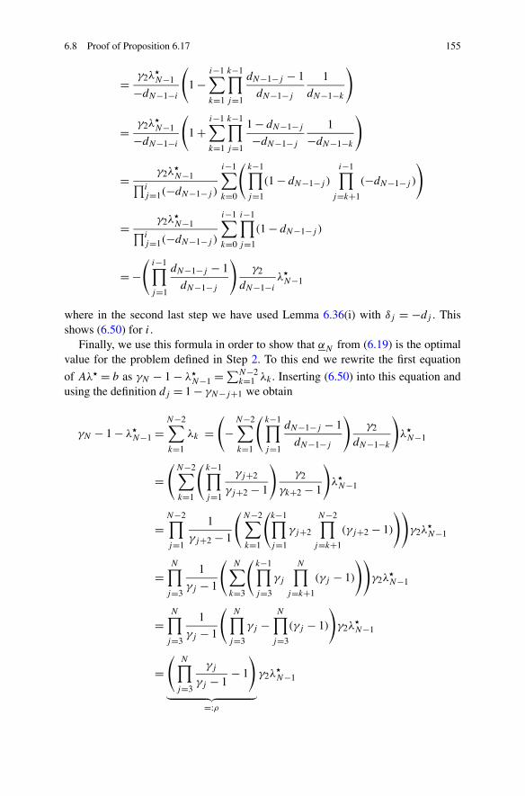
6.8 Proof of Proposition 6.17 155
= γ2λN−1
−dN−1−i
(
1 −i−1∑
k=1
k−1∏
j=1
dN−1−j − 1
dN−1−j
1
dN−1−k
)
= γ2λN−1
−dN−1−i
(
1 +i−1∑
k=1
k−1∏
j=1
1 − dN−1−j
−dN−1−j
1
−dN−1−k
)
= γ2λN−1∏i
j=1(−dN−1−j )
i−1∑
k=0
(k−1∏
j=1
(1 − dN−1−j )
i−1∏
j=k+1
(−dN−1−j )
)
= γ2λN−1
∏ij=1(−dN−1−j )
i−1∑
k=0
i−1∏
j=1
(1 − dN−1−j )
= −(
i−1∏
j=1
dN−1−j − 1
dN−1−j
)γ2
dN−1−i
λN−1
where in the second last step we have used Lemma 6.36(i) with δj = −dj . Thisshows (6.50) for i.
Finally, we use this formula in order to show that αN from (6.19) is the optimalvalue for the problem defined in Step 2. To this end we rewrite the first equation
of Aλ = b as γN − 1 − λN−1 =∑N−2
k=1 λk . Inserting (6.50) into this equation andusing the definition dj = 1 − γN−j+1 we obtain
γN − 1 − λN−1 =
N−2∑
k=1
λk =(
−N−2∑
k=1
(k−1∏
j=1
dN−1−j − 1
dN−1−j
)γ2
dN−1−k
)
λN−1
=(
N−2∑
k=1
(k−1∏
j=1
γj+2
γj+2 − 1
)γ2
γk+2 − 1
)
λN−1
=N−2∏
j=1
1
γj+2 − 1
(N−2∑
k=1
(k−1∏
j=1
γj+2
N−2∏
j=k+1
(γj+2 − 1)
))
γ2λN−1
=N∏
j=3
1
γj − 1
(N∑
k=3
(k−1∏
j=3
γj
N∏
j=k+1
(γj − 1)
))
γ2λN−1
=N∏
j=3
1
γj − 1
(N∏
j=3
γj −N∏
j=3
(γj − 1)
)
γ2λN−1
=(
N∏
j=3
γj
γj − 1− 1
)
︸ ︷︷ ︸=:ρ
γ2λN−1
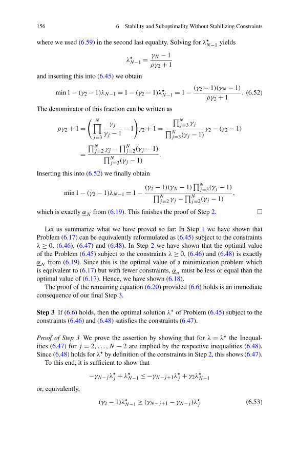
156 6 Stability and Suboptimality Without Stabilizing Constraints
where we used (6.59) in the second last equality. Solving for λN−1 yields
λN−1 = γN − 1
ργ2 + 1
and inserting this into (6.45) we obtain
min 1 − (γ2 − 1)λN−1 = 1 − (γ2 − 1)λN−1 = 1 − (γ2 − 1)(γN − 1)
ργ2 + 1. (6.52)
The denominator of this fraction can be written as
ργ2 + 1 =(
N∏
j=3
γj
γj − 1− 1
)
γ2 + 1 =∏N
j=3 γj∏N
j=3(γj − 1)γ2 − (γ2 − 1)
=∏N
j=2 γj −∏Nj=2(γj − 1)
∏Nj=3(γj − 1)
.
Inserting this into (6.52) we finally obtain
min 1 − (γ2 − 1)λN−1 = 1 − (γ2 − 1)(γN − 1)∏N
j=3(γj − 1)∏N
j=2 γj −∏Nj=2(γj − 1)
,
which is exactly αN from (6.19). This finishes the proof of Step 2. �
Let us summarize what we have proved so far: In Step 1 we have shown thatProblem (6.17) can be equivalently reformulated as (6.45) subject to the constraintsλ ≥ 0, (6.46), (6.47) and (6.48). In Step 2 we have shown that the optimal valueof the Problem (6.45) subject to the constraints λ ≥ 0, (6.46) and (6.48) is exactlyαN from (6.19). Since this is the optimal value of a minimization problem whichis equivalent to (6.17) but with fewer constraints, αn must be less or equal than theoptimal value of (6.17). Hence, we have shown (6.18).
The proof of the remaining equation (6.20) provided (6.6) holds is an immediateconsequence of our final Step 3.
Step 3 If (6.6) holds, then the optimal solution λ∗ of Problem (6.45) subject to theconstraints (6.46) and (6.48) satisfies the constraints (6.47).
Proof of Step 3 We prove the assertion by showing that for λ = λ the Inequal-ities (6.47) for j = 2, . . . ,N − 2 are implied by the respective inequalities (6.48).Since (6.48) holds for λ by definition of the constraints in Step 2, this shows (6.47).
To this end, it is sufficient to show that
−γN−jλj + λ
N−1 ≤ −γN−j+1λj + γ2λ
N−1
or, equivalently,
(γ2 − 1)λN−1 ≥ (γN−j+1 − γN−j )λ
j (6.53)

6.8 Proof of Proposition 6.17 157
holds for j = 2, . . . ,N − 2. Inserting (6.50) one sees that (6.53) is equivalent to
N−j+1∏
i=2
(γi − 1) ≥ (γN−j+1 − γN−j )
N−j∏
i=2
γi . (6.54)
Now we define cn := β(r, n)/r . Note that the cn are well defined since β is linearin r and that the identity γk =∑k−1
n=0 cn holds. Property (6.6) then implies1
cn+m ≤ cncm for all n,m ∈ N0. (6.55)
In order to prove (6.54) we prove the auxiliary inequality
N−j∏
i=2
(γi − 1)
N−j+k−1∑
n=k
cn − cN−j+k−1
N−j∏
i=2
γi ≥ 0 (6.56)
for arbitrary k ∈ N and j = 1, . . . ,N − 2 by induction over j , starting with j =N − 2. In this case for arbitrary k ∈ N we get
N−j∏
i=2
(γi − 1)
N−j+k−1∑
n=k
cn − cN−j+k−1
N−j∏
i=2
γi = (γ2 − 1)(ck + ck+1) − ck+1γ2
= γ2ck − ck − ck+1
= c0ck + c1ck − ck − ck+1
≥ ck + ck+1 − ck − ck+1 = 0
using (6.55) for m = k and n = 0 and 1 in the ≥-estimate. For the induction stepj + 1 → j and arbitrary k ∈ N we can write the right hand side of (6.56)
N−j∏
i=2
(γi − 1)
N−j+k−1∑
n=k
cn − cN−j+k−1
N−j∏
i=2
γi
= (−1)
N−j−1∏
i=2
(γi − 1)
N−j+k−1∑
n=k
cn
+ γN−j
[N−j−1∏
i=2
(γi − 1)
N−j+k−1∑
n=k
cn − cN−j+k−1
N−j−1∏
i=2
γi
]
=N−j−1∏
i=2
(γi − 1)
(
ckγN−j −N−j+k−1∑
n=k
cn
)
+ γN−j
[N−j−1∏
i=2
(γi − 1)
N−j+k−1∑
n=k+1
cn − cN−j+k−1
N−j−1∏
i=2
γi
]
.
1In fact, (6.55) is the reason for calling (6.6) “submultiplicativity”.

158 6 Stability and Suboptimality Without Stabilizing Constraints
Now the induction assumption implies that the second summand is ≥ 0, since theterm in square brackets is the right hand side of (6.56) with j + 1 and k + 1 insteadof j and k. For the first summand, using (6.55) we can estimate
ckγN−j = ck
N−j−1∑
n=0
cn =N−j−1∑
n=0
ckcn ≥N−j−1∑
n=0
ck+n =N−j+k−1∑
n=k
cn.
This shows that the term in brackets and thus the whole first summand is ≥ 0, whichproves (6.56).
Using the equality γk = ∑k−1n=0 ck and c0 ≥ 1, the left hand side of the desired
inequality (6.54) can be estimated by
N−j+1∏
i=2
(γi − 1) =N−j∏
i=2
(γi − 1)
(N−j∑
n=0
cn − 1
)
≥N−j∏
i=2
(γi − 1)
N−j∑
n=1
cn.
For the right hand side we obtain
(γN−j+1 − γN−j )
N−j∏
i=2
γi = cN−j
N−j∏
i=2
γi .
Hence, (6.56) for k = 1 implies (6.54) and thus (6.53). This proves Step 3. �
Step 3 implies that the optimal solution αN from (6.19) of (6.45) subject to theconstraints (6.46) and (6.48) obtained in Step 2 equals the optimal solution of (6.45)subject to the constraints (6.46), (6.47) and (6.48). Since by Step 1 the latter prob-lem is equivalent to (6.17), this proves (6.20) and thus finishes the proof of Propo-sition 6.17.
Remark 6.35 In Step 3 we have shown that under the condition (6.6) the conditions(6.47) are redundant in (6.45). Since in Step 1 we have shown that the conditions(6.47) are equivalent to (6.11) for k = 1, . . . ,N − 2, this shows that under condition(6.6) the optimal value of Problem (6.17) does not change if we remove the con-straints (6.11) for k = 1, . . . ,N − 2. While this has no consequences for the resultsin this book—since we get these constraints for free from the optimality of the tra-jectory xu(·, x0) via Lemma 6.10—this observation may be useful in other settings,e.g., when analyzing NMPC with nonoptimal trajectories.
We end this section with a technical lemma we needed in the preceding proof.
Lemma 6.36
(i) For all δ1, . . . , δN−2 ∈ R and all i ∈ {1, . . . ,N − 1} the equation
i−1∏
j=1
(1 + δN−1−j ) =i−1∑
k=0
(k−1∏
j=1
(1 + δN−1−j )
i−1∏
j=k+1
δN−1−j
)
. (6.57)
holds (with the usual convention∏j2
j=j1= 1 if j2 < j1).

6.9 Notes and Extensions 159
(ii) For all δ ∈ R and k ∈ {1, . . . ,N − 1} the equation
(1 + δ)N−1−k =N−2−k∑
n=0
(1 + δ)N−2−k−nδn + δN−1−k (6.58)
holds.(iii) For all γ3, . . . , γN ∈ R the equation
N∏
j=3
γj =N∏
j=3
(γj − 1) +N∑
k=3
(k−1∏
j=3
γj
N∏
j=k+1
(γj − 1)
)
(6.59)
holds.
Proof (i) We prove (6.57) by induction over i. For i = 1 the equality is obvious.Under the induction assumption that (6.57) holds for i − 1 instead of i we obtain
i−1∏
j=1
(1 + δN−1−j ) =i−2∏
j=1
(1 + δN−1−j ) + δN−1−(i−1)
(i−1)−1∏
j=1
(1 + δN−1−j )
=i−2∏
j=1
(1 + δN−1−j )
+ δN−1−(i−1)
(i−1)−1∑
k=1
(k−1∏
j=1
(1 + δN−1−j )
(i−1)−1∏
j=k+1
δN−1−j
)
=i−1∑
k=0
(k−1∏
j=1
(1 + δN−1−j )
i−1∏
j=k+1
δN−1−j
)
,
i.e., (6.57) for i.(ii) Formula (6.58) follows immediately from (6.57) by setting δ1 = · · · =
δN−1 = δ and k = N − i.(iii) Using (6.57) with δN−1−j = γj+2 − 1 and i = N − 1 yields
N−2∏
j=1
γj+2 =N−2∑
k=0
(k−1∏
j=1
γj+2
N−2∏
j=k+1
(γj+2 − 1)
)
.
Writing the summand for k = 0 on the right hand side separately and using thesummation indices j + 2 instead of j and k + 2 instead of k yields (6.59). �
6.9 Notes and Extensions
The conceptual idea of establishing stability and performance of NMPC schemesvia relaxed dynamic programming ideas as outlined in Sect. 6.1 was to our knowl-edge first used by Shamma and Xiong [11]. However, in this reference different

160 6 Stability and Suboptimality Without Stabilizing Constraints
inequalities from (5.1) were used and the inequalities were verified by numericalevaluation. In the form presented here, relaxed dynamic programming was intro-duced for the analysis of NMPC schemes in Grüne and Rantzer [6], where also afirst controllability condition for verifying this inequality was given.
The asymptotic controllability condition with respect to � from Sect. 6.2 was in-troduced in Grüne [5] and most of the results in Sects. 6.2–6.5 were taken from thisreference with minor modifications and extensions. Exceptions are Proposition 6.17and Theorem 6.21 and their respective proofs, which were taken from Grüne, Pan-nek, Seehafer and Worthmann [7]. Note that in [7] Proposition 6.17 is proved in amore general setting (and with an even more involved proof); we will sketch thissetting in Sect. 7.4.
Section 6.6 summarizes and extends discussions from [5] and [7]. Example 6.26in this section has not been published before while Example 6.27 was taken fromAltmüller, Grüne and Worthmann [2]. Sect. 6.7 consists of previously unpublishedmaterial, however, the semiglobal practical stability result in Theorem 6.33 wasproved before by Grimm, Messina, Tuna and Teel in [4, Theorem 1] using a dif-ferent proof technique and slightly different technical assumptions. Corollaries 2and 3 in [4] provide counterparts of Theorems 6.31 and 6.21 proving semiglobaland “real” asymptotic stability, respectively, under similar conditions as in our The-orems. Since the results in this reference are quite similar to our approach presentedin this chapter, we will briefly discuss the main differences.
The decisive difference to our results is that in [4] bounds of the type VN(x) ≤αV (|x|x∗) for αV ∈ K∞ independent of N together with suitable bounds on αV andthe other K∞ functions involved are used while our analysis relies on the Assump-tions 6.4 or 6.30. The main advantage of using these assumptions instead of thebound VN(x) ≤ αV (|x|x∗) lies in the fact that the fine structure of β(r, k) or Bk—in particular the dependence of these functions on k—can be used. The benefit ofusing this structure is nicely illustrated in the exponential controllability case (6.3):for β(r, k) = Cσkr and �∗(x) ≤ α4(|x|x∗) we obtain the bound VN(x) ≤ αV (|x|x∗)for αV (r) = Cα4(r)/(1 − σ). Given C1 < C2 and σ1 > σ2 with
C1
1 − σ1= C2
1 − σ2
this will thus yield the same αV . Hence, using the upper bound αV in the stabilityanalysis, we cannot distinguish between large overshoot C2 and fast decay σ2 andsmall overshoot C1 and slow decay σ1. However, our analysis in Sect. 6.6 based onAssumption 6.4 shows that the pair C1, σ1 provides a much better stability behaviorthan C2, σ2. Particularly, Fig. 6.1 shows that for C1 sufficiently close to 1 we alwaysenter the region where stability holds for N = 2, a fact which remains invisible whenlooking only at αV .
Another advantage of our approach is that it automatically leads to suboptimalityestimates which are not provided in [4]. On the other hand, a major advantage of theapproach in [4] is that it allows us to handle nonpositive definite running costs � viaa suitable detectability condition. We will discuss this aspect in Sect. 7.3.
Besides the approach presented in this chapter and [4] there are various otherapproaches which ensure stability of NMPC schemes without stabilizing terminal

6.10 Problems 161
constraints and terminal cost. Probably the earliest reference is Alamir and Bornard[1], another well known reference is Jadbabaie and Hauser [8]. Both have alreadybriefly been discussed at the end of Sect. 6.1; here we only remark that these refer-ences do not provide bounds on the optimization horizon N .
We finally mention that inverse optimality in the sense of Theorem 5.24 doesin general not hold for problems without stabilizing terminal constraints, since themodified running cost used in Theorem 5.24 may become negative, see Problem 6,below.
6.10 Problems
General remark: all NMPC algorithms in the following problems are meant withoutstabilizing terminal constraints.
1. Consider a control system (2.1) on X = Rd and U = R
m which is exponentiallycontrollable to x∗ = 0. This means that there exist constants K > 0 and η ∈ (0,1)
such that for each x ∈ Rd there is a control sequence ux ∈ U
N(x) such that∥∥xux
(k, x)∥∥≤ Kηn‖x‖
holds for all k ∈ N0.(a) Show that the system satisfies the Controllability Assumption 6.4 with β ∈
K L0 of type (6.3) for any running cost of the form �(x,u) = x�Qx withpositive definite matrix Q ∈ R
d×d .(b) Does the assertion from (a) also hold for a running cost of the form �(x,u) =
x�Qx + u�Ru for positive definite matrices Q ∈ Rd×d and R ∈ R
m×m? Ifnot, which additional property must be satisfied?
Hint: Look at the hints for Problem 2 in Chap. 4.2. Consider a function β ∈ K L0 of the form (6.4).
(a) Prove that there exist C ≥ 1 and σ ∈ (0,1) such that for the function β ∈ K L0
of type (6.3) with β(r, n) = Cσnr the inequality
β(r, n) ≤ β(r, n)
holds for all n ∈ N0 and all r ≥ 0.(b) Determine C ≥ 1 and σ ∈ (0,1) (with C as small as possible) such that the
inequality from (a) holds for the values n0 = 2, c0 = 2 and c1 = 1 in (6.4).(c) Compute α for β(r, n) and β(r, n) for the values from (b) and N = 3,4,5,6
using (6.20) (MAPLE or MATLAB may be helpful here). Which functionprovides better values?
3. Consider the control system
x(n + 1) =(
1 1.1−1.1 1
)x(n) +
(01
)u(n)
with x(n) ∈ X = R, u(n) ∈ U = R and running cost �(x,u) = max{‖x‖∞, u}.

162 6 Stability and Suboptimality Without Stabilizing Constraints
(a) Given the initial value x(0) = (x1, x2), use the control sequence u(0) =21110x1 − 2x2, u(1) = 221
110x1 + 221100x2, u(n) = 0 for all n ≥ 2 to compute the
minimal horizon length N for which stability can be guaranteed.(b) Try to reduce the minimal required horizon length N from (a). To this end,
change the term u in the running cost � to ηu for some η ∈ R+0 and analyze
the impact of this change.Hint for (a): Construct β such that Assumption 6.4 holds and Corollary 6.19 isapplicable.
4. Consider a control system (2.1), an admissible feedback law μ : X → U anda Lyapunov function V : X → R
+0 for the closed-loop system x+ = g(x) :=
f (x,μ(x)). Show that the NMPC-feedback law μN for running cost �(x,u) =V (x) stabilizes the system for N = 2.
Hint: A direct argument may be easier than trying to apply one of the theoremsfrom this chapter.
5. Consider the control system
x(n + 1) = 2x(n) + u(n)
with x(n) ∈ X = R, u(n) ∈ U = R.(a) Show that for running cost �(x,u) = x2 the NMPC control law μN : X → U
is optimal for the infinite horizon problem for arbitrary N ≥ 2.(b) For the running cost �(x,u) = x2 + u2, compute minimal horizon lengths N
such that α ≥ α holds in (5.1) for α ∈ {0.5,0.9,0.99}.6. Consider the modified running cost function
�(x, u) := �(x,u) + VN−1(f (x,u)
)− VN
(f (x,u)
)
which we used for the inverse optimality statement in Chap. 5, cf. (5.32). Con-sider the NMPC problem x+ = x/2 + u2, X = X = U = U = R and �(x) = x2
without stabilizing terminal constraints and prove that for each N ≥ 2 the func-tion � is not of the form (3.2).
References
1. Alamir, M., Bornard, G.: Stability of a truncated infinite constrained receding horizon scheme:the general discrete nonlinear case. Automatica 31(9), 1353–1356 (1995)
2. Altmüller, N., Grüne, L., Worthmann, K.: Performance of NMPC schemes without stabiliz-ing terminal constraints. In: Diehl, M., Glineur, F., Jarlebring, E., Michiels, W. (eds.) RecentAdvances in Optimization and Its Applications in Engineering, pp. 289–298. Springer, Berlin(2010)
3. Altmüller, N., Grüne, L., Worthmann, K.: Receding horizon optimal control for the waveequation. In: Proceedings of the 49th IEEE Conference on Decision and Control – CDC 2010,Atlanta, Georgia, pp. 3427–3432 (2010)
4. Grimm, G., Messina, M.J., Tuna, S.E., Teel, A.R.: Model predictive control: for want of alocal control Lyapunov function, all is not lost. IEEE Trans. Automat. Control 50(5), 546–558(2005)
5. Grüne, L.: Analysis and design of unconstrained nonlinear MPC schemes for finite and infinitedimensional systems. SIAM J. Control Optim. 48, 1206–1228 (2009)

References 163
6. Grüne, L., Rantzer, A.: On the infinite horizon performance of receding horizon controllers.IEEE Trans. Automat. Control 53, 2100–2111 (2008)
7. Grüne, L., Pannek, J., Seehafer, M., Worthmann, K.: Analysis of unconstrained nonlinearMPC schemes with varying control horizon. SIAM J. Control Optim. 48, 4938–4962 (2010)
8. Jadbabaie, A., Hauser, J.: On the stability of receding horizon control with a general terminalcost. IEEE Trans. Automat. Control 50(5), 674–678 (2005)
9. Khalil, H.K.: Nonlinear Systems, 3rd edn. Prentice Hall, Upper Saddle River (2002)10. Nešic, D., Teel, A.R.: A framework for stabilization of nonlinear sampled-data systems based
on their approximate discrete-time models. IEEE Trans. Automat. Control 49(7), 1103–1122(2004)
11. Shamma, J.S., Xiong, D.: Linear nonquadratic optimal control. IEEE Trans. Automat. Control42(6), 875–879 (1997)
12. Sontag, E.D.: Comments on integral variants of ISS. Systems Control Lett. 34, 93–100 (1998)


Chapter 7Variants and Extensions
The results developed so far in this book can be extended in many ways. In thischapter we present a selection of possible variants and extensions. Some of theseintroduce new combinations of techniques developed in the previous chapters, oth-ers relax some of the previous assumptions in order to obtain more general resultsor strengthen assumptions in order to derive stronger results. Several sections con-tain algorithmic ideas which can be added on top of the basic NMPC schemes fromthe previous chapters. Parts of this chapter contain results which are somewhat pre-liminary and are thus subject to further research. Some sections have a survey likestyle and, in contrast to the other chapters of this book, proofs are occasionally onlysketched with appropriate references to the literature.
7.1 Mixed Constrained–Unconstrained Schemes
The previous Chaps. 5 and 6 have featured two extreme cases, namely NMPCschemes with terminal constraints X0 and costs F on the one hand and schemeswithout both X0 and F on the other hand. However, it appears natural to consideralso intermediate or mixed cases, namely schemes in which (nonequilibrium) ter-minal constraint sets X0 but no terminal costs F are used and schemes in whichterminal costs F but no terminal constraints sets X0 are used.
Schemes with terminal constraints X0 but without terminal costs F appear as aspecial case of Algorithm 3.10 (or its time varying counterpart 3.11) with (OCPN,e)= (5.15) and F ≡ 0. For this setting, it is not reasonable to expect that Assump-tion 5.9(ii) holds. Consequently, the argument used in the proof of Theorem 5.13does not apply; in fact, we are not aware of results in the literature analyzing suchschemes with the techniques from Chap. 5.
Fortunately, the stability analysis in Chap. 6 provides a remedy to this problem.Observe that the main structural assumption on the control sequences from Assump-tion 6.4 needed in the fundamental Lemmas 6.9 and 6.10 in Chap. 6 is that eachadmissible control sequence u ∈ U
N(x) can be extended to an admissible control
L. Grüne, J. Pannek, Nonlinear Model Predictive Control,Communications and Control Engineering,DOI 10.1007/978-0-85729-501-9_7, © Springer-Verlag London Limited 2011
165

166 7 Variants and Extensions
sequence u ∈ UN+K(x) for each K ≥ 1. Since Lemma 5.2(i) ensures this property
for UNX0
(x) provided X0 is viable, we can incorporate the terminal constraint set X0into the analysis from Chap. 6.
As a consequence, replacing UN(x) by U
NX0
(x) in Assumption 6.4 and assum-ing Assumption 5.9(i), i.e., viability of X0, all results in Chap. 6 carry over to thescheme with terminal constraint set. In particular, the stability results Theorem 6.18,Corollary 6.19, Theorem 6.21 and Theorem 6.33 remain valid. However, like in The-orem 5.13 the resulting controller μN is only defined on the feasible set XN fromDefinition 3.9.
This combined scheme inherits certain advantages and disadvantages from bothschemes. From the terminal constrained scheme we inherit that the resulting con-troller μN is only defined on the feasible set XN . On the other hand, as discussedbefore Lemma 5.3, we do not need to assume viability of X but only for the termi-nal constraint set X0 (further methods to avoid the viability assumption on X willbe discussed in Sects. 8.1–8.3).
From the unconstrained scheme we inherit the advantage that no terminal costsatisfying Assumption 5.9(ii) needs to be constructed. On the other hand, we needto ensure that the assumptions of one of the mentioned stability results from Chap. 6hold whose rigorous verification may be involved, cf. also Sect. 6.6. For a more com-prehensive discussion on advantages and disadvantages of different NMPC schemeswe refer to Sect. 8.4.
Another way of imposing terminal constraints without terminal costs which canbe found in the literature is via so-called contractive constraints. Here the termi-nal constraint set depends on the initial value x0 of the optimal control problem(OCPN,e) via
X0 = {x ∈ X
∣∣ |x|x∗ ≤ γ |x0|x∗}
for some constant γ ∈ (0,1); see, e.g., the book of Alamir [1] or the works of deOliveira Kothare and Morari [28] and De Nicolao, Magni and Scattolini [5]. How-ever, for these constraints stability is only guaranteed if either the whole optimalcontrol sequence (as opposed to only the first element) is applied or if the optimiza-tion horizon is treated as an optimization variable and the contractivity condition isincorporated into the optimization objective [1, Chap. 4]. Since these approaches donot conform with the MPC paradigm used throughout this book, we do not discusstheir analysis in detail.
Schemes with terminal cost F but without terminal constraint X0 have been in-vestigated in several places in the literature, for instance in Grimm, Messina, Tunaand Teel [13] and Jadbabaie and Hauser [22] (for more information on these ref-erences see also the discussions at the end of Sect. 6.1 and in Sect. 6.9). In bothreferences stability results for such schemes are derived in which only positive defi-niteness of F is assumed. Roughly speaking, these references show that the additionof F does not destroy stability. While the authors emphasize the potential positiveeffects of adding such costs, they do not rigorously analyze these positive effects.In contrast to this, in the work of Parisini and Zoppoli [30] the specific properties ofthe terminal cost described in Remark 5.15 were exploited in order to show stability.

7.1 Mixed Constrained–Unconstrained Schemes 167
The proof in [30] uses that under suitable conditions and for sufficiently large opti-mization horizon N for all initial values from a given region the open-loop optimaltrajectories end up in the terminal constraint set without actually imposing this as acondition. The same proof idea has been generalized later by Limón, Alamo, Salasand Camacho [24] for a more general terminal cost.
Here we outline an approach from Grüne and Rantzer [17] which we combinewith the analysis technique from Chap. 6. This approach rigorously shows the pos-itive effect of adding a terminal cost also in the absence of stabilizing terminal con-straints. In contrast to [30] or [24] the stability property is not restricted to sets ofinitial values for which the open-loop optimal trajectories end up in a terminal con-straint set. However, the fact that this happens for a set of initial values around theorigin will be used in our proof. We start from a terminal cost function F satisfy-ing Assumption 5.9(ii) with a forward invariant neighborhood X0 of x∗, however,we will not use X0 as a terminal constraint set. Instead, we assume that F ≡ c > 0holds on the boundary ∂X0 with c ≥ supx∈X0
F(x). This is, for instance, satisfied ifF is constructed from a linearization via linear–quadratic techniques according toRemark 5.15 and X0 is a sublevel set of F . Then we may extend F continuously tothe whole set X by setting F(x) := c for all x ∈ X \ X0.
With this setting we obtain the following theorem.
Theorem 7.1 Let the assumptions of Theorem 6.33 be satisfied for the NMPC Algo-rithm 3.1 without terminal cost. Let F : X → R
+0 and assume that Assumption 5.9
holds for some set X0 containing a ball Bη(x∗) for some η > 0. Assume, further-more, that F ≡ c holds outside X0 with c ≥ supx∈X0
F(x) and that F(x) ≤ α2(|x|x∗)holds for all x ∈ X0 and some α2 ∈ K∞. Consider the NMPC Algorithm 3.10 with(OCPN,e) = (5.15) for this F but without terminal constraints, i.e., with X0 = X
in (5.15).Then the nominal NMPC closed-loop system (3.5) with NMPC feedback law μN
is semiglobally asymptotically stable on X with respect to the parameter N in thesense of Definition 6.28(i).
Proof We consider the following three optimal control problems
(a) (5.15) with X0 = X, which generates μN in this theorem(b) (5.15) with X0 from Assumption 5.9 for F , which generates μN in Theorem 5.5(c) (OCPN), which generates μN in Theorem 6.18
and denote the respective optimal value functions by V(a)N , V
(b)N and V
(c)N . For each
x ∈ X we obtain the inequalities V(c)N (x) ≤ V
(a)N (x) ≤ V
(c)N (x) + c and, for x ∈ XN
(where XN denotes the feasible set from Definition 3.9 for Problem (b)), we haveV
(a)N (x) ≤ V
(b)N (x).
In order to show semiglobal asymptotic stability, i.e., Definition 6.28(i), we fix� > 0. For an arbitrary x ∈ X we consider the optimal control u� for Problem (a)(which implies μN(x) = u�(0) for μN from this theorem) and distinguish two cases:

168 7 Variants and Extensions
(i) xu�(N,x) ∈ X0: This implies u� ∈ UNX0
(x) and hence x ∈ XN and V(a)N (x) =
V(b)N (x). Using xu�(1, x) = f (x,μN(x)) ∈ XN and V
(a)N ≤ V
(b)N on XN , the proof
of Theorem 5.5 yields
V(a)N (x) = V
(b)N (x) ≥ �
(x,μN(x)
) + V(b)N
(f
(x,μN(x)
))
≥ �(x,μN(x)
) + V(a)N
(f
(x,μN(x)
)). (7.1)
This inequality will be used below in order to conclude asymptotic stability. Beforewe turn to case (ii) we show that case (i) applies to all points x ∈ Bδ(x∗) for someδ > 0:
Since (5.20) shows V(b)N (x) ≤ F(x) on X0, we obtain V
(a)N (x) ≤ V
(b)N (x) ≤
α2(|x|x∗) for x ∈ Bη(x∗) ⊆ X0. For δ = min{η, α−12 (c/2)} this implies V
(a)N (x) ≤
c/2 for all x ∈ Bδ(x∗). On the other hand, xu�(N,x) /∈ X0 implies F(xu�(N,x)) = c
and thus V(a)N (x) ≥ c. Hence, case (i) occurs for all x ∈ Bδ(x∗).
(ii) xu�(N,x) /∈ X0: This implies F(xu�(N,x)) = c and thus V(a)N (x) = V
(c)N (x)+
c. This implies that u� is an optimal control for V(c)N (x) and from the proof of The-
orem 6.33 we obtain that (5.1), i.e.,
V(c)N (x) ≥ α�
(x,μN(x)
) + V(c)N
(f
(x,μN(x)
))
holds for all x ∈ Y = S \ P with S and P chosen as in the proof of Theorem 6.33.The sets S and P are forward invariant and by choosing N ∈ N sufficiently largewe obtain α > 0, B�(x∗) ⊆ S and P ⊂ Bδ(x∗) for � fixed above and δ definedat the end of case (i). Since V
(a)N (x) = V
(c)N (x) + c and V
(a)N (f (x,μN(x))) ≤
V(c)N (f (x,μN(x))) + c we obtain
V(a)N (x) ≥ α�
(x,μN(x)
) + V(a)N
(f
(x,μN(x)
))(7.2)
for all y ∈ Y and some α > 0.Now, the choice of N and P implies that for x ∈ S \ Bδ(x∗) Inequality (7.2)
holds while for x ∈ Bδ(x∗) Inequality (7.1) holds. This implies that Theorem 4.14is applicable with S(n) = S which yields semiglobal practical stability usingLemma 6.29(i). �
Comparing Theorem 7.1 with Theorem 6.33, one sees that the benefit of includ-ing the terminal cost F is that here we obtain semiglobal asymptotic stability whilewithout F we can only guarantee semiglobal practical asymptotic stability. Looselyspeaking, the unconstrained scheme guarantees stability up to the neighborhoodBδ(x∗), while F ensures asymptotic stability inside this neighborhood.
7.2 Unconstrained NMPC with Terminal Weights
Our next extension analyzes the effect of inclusion of terminal weights in (OCPN),i.e., in NMPC schemes without stabilizing terminal constraints and costs. Both in

7.2 Unconstrained NMPC with Terminal Weights 169
numerical simulations and in practice one can observe that adding terminal weightscan improve the stability behavior of the NMPC closed loop. Formally, adding ter-minal weights can be achieved by replacing the optimization criterion in (OCPN)by
JN
(x0, u(·)) :=
N−2∑
k=0
�(xu(k, x0), u(k)
) + ω�(xu(N − 1, x0), u(N − 1)
)(7.3)
for some ω ≥ 1. For ω = 1 we thus obtain the original problem (OCPN). This exten-sion is a special case of (OCPN,e) in which we specify X0 = X, F ≡ 0, ω1 = ω andω2 = ω3 = · · · = ωN = 1. In a similar way, such a terminal weight can be added tothe respective time variant problem (OCPn
N) leading to a special case of (OCPnN,e).
Thus, all results developed in Chap. 3 apply to this problem. Given that the optimalcontrol value u(N − 1) in (7.3) will minimize �(xu(N − 1, x0), u(N − 1)), this ap-proach is identical to choosing F(x) = ω�∗(x) and N = N − 1 in the terminal costapproach discussed in the previous section, with �∗ from (6.2). However, the spe-cific structure of the terminal cost allows for applying different and more powerfulanalysis techniques which we explain now.
The terminal weight leads to an increased penalization of �(xu(N −1, x0), u(N −1)) in JN and thus to an increased penalization of the distance of xu(N − 1, x0) tox∗. Thus, for ω > 1 the optimizer selects a finite time optimal trajectory whoseterminal state xu�(N − 1, x0) has a smaller distance to x∗. Since our goal is that theNMPC-feedback law μN steers the trajectory to x∗, this would intuitively explainbetter stability behavior.
Formally, however, the analysis is not that easy because in closed loop we neveractually apply u�(1), . . . , u�(N −1) and the effect of ω on u�(0) is not that obvious.Hence, we extend the technique developed in Chap. 6 in order to analyze the effectof ω. To this end, we change the definition (6.8) of BN to
BN(r) :=N−2∑
n=0
β(r, n) + ωβ(r,N − 1).
With this definition, all results in Sect. 6.3 remain valid for the extended problem.Proposition 6.12 remains valid, too, if we change (6.11) to
N−2∑
n=k
λn + ωλN−1 ≤ BN−k(λk), k = 0, . . . ,N − 2.
If, furthermore, in the subsequent statements we replace∑N−1
n=0 λn by∑N−2
n=0 λn +ωλN−1, then it can be shown that Proposition 6.17 remains valid if we replace (6.19)by
αωN := 1 − (γN − 1)(γ2 − ω)
∏Ni=3(γi − 1)
∏Ni=2 γi − (γ2 − ω)
∏Ni=3(γi − 1)
. (7.4)
The proof is similar to the proof of Proposition 6.17 and can be found in Grüne,Pannek, Seehafer and Worthmann [20].

170 7 Variants and Extensions
Fig. 7.1 Suboptimality indexα depending on terminalweight ω
With this expression, Theorem 6.18 and its corollaries remain valid, except forthe inequalities VN(x)/α ≤ V∞(x)/α and CVN(x) ≤ CV∞(x), which do in generalno longer hold because of the additional weight which is present in VN but notin V∞.
Figure 7.1 shows the values from (7.4) for an exponential β of type (6.3)with C = 2 and σ = 0.55, optimization horizon N = 5 and terminal weightsω = 1,2, . . . ,20. The figure illustrates that our analysis reflects the positive effectthe terminal weight has on the stability: while for ω = 1,2 we obtain negative val-ues for α and thus stability cannot be ensured, for ω ≥ 3 stability is guaranteed.However, one also sees that for ω ≥ 10 the value of α is decreasing, again. For moreexamples for the effect of terminal weights we refer to [20] and Example 7.14, be-low.
7.3 Nonpositive Definite Running Cost
In many regulator problems one is not interested in driving the whole state to areference trajectory or point. Rather, often one is only interested in certain outputquantities. The following example illustrates such a situation.
Example 7.2 We reconsider Example 2.2, i.e.,(
x+1
x+2
)=
(x1 + x2 + u/2
x2 + u
)=: f (x,u)
with running cost
�(x,u) = x21 + u2.
In contrast to our standing assumption (3.2), no matter how we choose x∗ ∈ R2, this
function does not satisfy �(x,u) > 0 for all x ∈ X and u ∈ U with x �= x∗. Instead,
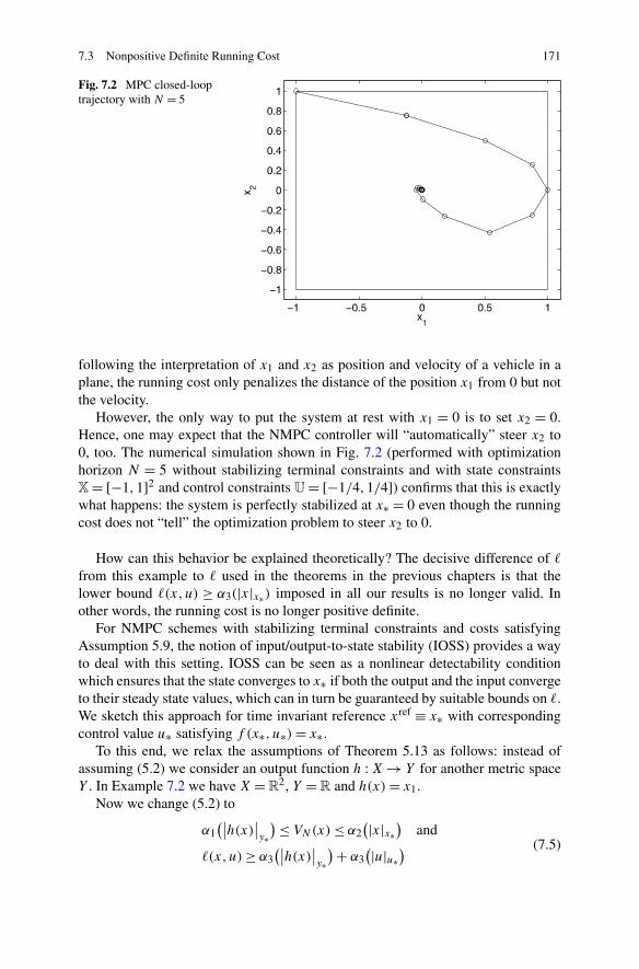
7.3 Nonpositive Definite Running Cost 171
Fig. 7.2 MPC closed-looptrajectory with N = 5
following the interpretation of x1 and x2 as position and velocity of a vehicle in aplane, the running cost only penalizes the distance of the position x1 from 0 but notthe velocity.
However, the only way to put the system at rest with x1 = 0 is to set x2 = 0.Hence, one may expect that the NMPC controller will “automatically” steer x2 to0, too. The numerical simulation shown in Fig. 7.2 (performed with optimizationhorizon N = 5 without stabilizing terminal constraints and with state constraintsX = [−1,1]2 and control constraints U = [−1/4,1/4]) confirms that this is exactlywhat happens: the system is perfectly stabilized at x∗ = 0 even though the runningcost does not “tell” the optimization problem to steer x2 to 0.
How can this behavior be explained theoretically? The decisive difference of �
from this example to � used in the theorems in the previous chapters is that thelower bound �(x,u) ≥ α3(|x|x∗) imposed in all our results is no longer valid. Inother words, the running cost is no longer positive definite.
For NMPC schemes with stabilizing terminal constraints and costs satisfyingAssumption 5.9, the notion of input/output-to-state stability (IOSS) provides a wayto deal with this setting. IOSS can be seen as a nonlinear detectability conditionwhich ensures that the state converges to x∗ if both the output and the input convergeto their steady state values, which can in turn be guaranteed by suitable bounds on �.We sketch this approach for time invariant reference xref ≡ x∗ with correspondingcontrol value u∗ satisfying f (x∗, u∗) = x∗.
To this end, we relax the assumptions of Theorem 5.13 as follows: instead ofassuming (5.2) we consider an output function h : X → Y for another metric spaceY . In Example 7.2 we have X = R
2, Y = R and h(x) = x1.Now we change (5.2) to
α1(∣∣h(x)
∣∣y∗
) ≤ VN(x) ≤ α2(|x|x∗
)and
�(x,u) ≥ α3(∣∣h(x)
∣∣y∗
) + α3(|u|u∗
) (7.5)

172 7 Variants and Extensions
with y∗ = h(x∗) and |h(x)|y∗ = dY (h(x), y∗), where dY (·,·) is the metric on Y . Fur-thermore, we assume that the system with output y = h(x) is IOSS in the followingsense: There exist β ∈ K L and γ1, γ2 ∈ K∞ such that for each x ∈ X and eachadmissible control u ∈ U
∞(x) the inequality∣∣xu(n, x)
∣∣x∗ ≤ max
{β(|x|x∗, n
), γ1
(max
k=0,...,n−1
∣∣u(k)∣∣u∗
),
γ2
(max
k=0,...,n−1
∣∣y(k)∣∣y∗
)}
holds for all n ∈ N0 with y(k) = h(xu(k, x)).With these changed assumptions, the assertion of Theorem 5.13 remains valid.
The proof relies on the fact that the function VN still satisfies
VN(x) ≥ �(x,μN(x)
) + VN
(f
(x,μN(x)
)).
This implies that VN(xμN(n, x)) is monotone decreasing in n and since it is bounded
from below by 0 it converges to some value as n → ∞, although not neces-sarily to 0. However, the convergence of VN(xμN
(n, x)) implies convergence of�(xμN
(n, x),μN(xμN(n, x))) → 0 which by means of the last inequality in (7.5)
yields h(xμN(n, x)) → 0 and μN(xμN
(n, x)) → 0. Now the IOSS property can beused to conclude asymptotic stability of the closed loop. For more details of thisapproach, we refer to the book of Rawlings and Mayne [31, Sect. 2.7 and the refer-ences therein].
While the approach just sketched relies on stabilizing terminal constraints, thesimulation in Example 7.2 shows that asymptotic stability can also be expectedwithout such constraints. For this setting, a stability proof was given in the work ofGrimm, Messina, Tuna and Teel [13] and the main result in this reference extendsTheorem 6.33. Again, a detectability condition is used, but this time it is formu-lated via a suitable auxiliary function W : we assume the existence of a functionW : X → R
+0 which satisfies the inequalities
W(x) ≤ αW
(|x|x∗),
W(f (x,u)
) − W(x) ≤ −αW
(|x|x∗) + γW
(�(x,u)
) (7.6)
for all x ∈ X, u ∈ U(x) and suitable functions αW ,αW ,γW ∈ K∞. In turn, weremove the lower bound α3(|x|x∗) ≤ �∗(x) for �∗ from (6.2) from the assumptionsof Theorem 6.33. Observe that whenever this lower bound holds, the detectabilitycondition is trivially satisfied with W ≡ 0, γW (r) = r and αW = α3.
Under these modified assumptions, it is shown in [13, Theorem 1] that thesemiglobal practical stability assertion of Theorem 6.33 remains valid. Furthermore,[13, Corollary 2 and Corollary 3] provide counterparts to Theorems 6.31 and 6.21which prove semiglobal and “real” asymptotic stability, respectively. In contrast tothe IOSS-based result for stabilizing terminal constraints, the proof of [13, Theo-rem 1] yields a Lyapunov function constructed from the optimal value function VN
and the function W from the detectability condition. In the simplest case, which oc-curs under suitable bounds on the involved K∞-functions, this Lyapunov functionis given by VN + W . In general, a weighted sum has to be used.

7.3 Nonpositive Definite Running Cost 173
In Example 7.2, numerical evaluation suggests that the detectability condition issatisfied for W(x) = max{−|x1x2|+x2
2 ,0}/2 and γW (r) = r . Plots of the differenceW(x) − W(f (x,u)) + �(x,u) in MAPLE indicate that this expression is positivedefinite and can hence be bounded from below by some function αW (|x|x∗); a rig-orous proof of this property is, however, missing up to now.
As discussed in Sect. 6.9, the analysis in [13] uses a condition of the formVN(x) ≤ αV (r) in order to show stability, which compared to our Assumptions 6.4or 6.30 has the drawback to yield fewer information for the design of “good” run-ning costs �. Furthermore, suboptimality estimates are not easily available. It wouldhence be desirable to extend the statement and proof of Theorem 6.18 to the caseof nonpositive definite running costs. A first attempt in this direction is the follow-ing: suppose that we are able to find a function W : X → R
+0 satisfying (7.6) with
γW (r) = r . Then the function
�W (x,u) := W(x) − W(f (x,u)
) + �(x,u)
satisfies a lower bound of the form
�∗W (x) := min
u∈U�W (x,u) ≥ αW
(|x|x∗)
for all x ∈ X. Let u� be an optimal control for VN(x), i.e.,
VN(x) = JN
(x,u�
) =N−1∑
k=0
�(xu�(k, x), u�(k)
)
and define
VN (x) :=N−1∑
k=0
�W
(xu�(k, x), u�(k)
).
The definition of �W then implies
VN (x) = W(x) − W(xu�(N,x)
) + VN(x).
Changing the inequality in Assumption 6.30 to
Vk(x) ≤ Bk
(�∗W (x)
) − W(x)
then implies
Vk(x) ≤ Bk
(�∗W(x)
).
Using this inequality, it should be possible to carry over all results in Sect. 6.3 to VN
using �W in place of �. A rigorous investigation of this approach as well as possibleextensions will be the topic of future research.
In this context we would like to emphasize once again that even if the runningcost � only depends on an output y, the resulting NMPC-feedback law is still a statefeedback law because the full state information is needed in order to compute theprediction xu(·, x0) for x0 = x(n).

174 7 Variants and Extensions
7.4 Multistep NMPC-Feedback Laws
Next we investigate what happens if instead of only the first control value u�(0) weimplement the first m values u�(0), . . . , u�(m − 1) before optimizing again. For-mally, we can write this NMPC variant as a multistep feedback law
μN(x, k) := u�(k), k = 0, . . . ,m − 1,
where u� is an optimal control sequence for problem (OCPN,e) (or one of its vari-ants) with initial value x0 = x. The resulting generalized closed-loop system thenreads
x(n + 1) = f(x(n),μN
(x([n]m
), n − [n]m
)), (7.7)
where [n]m denotes the largest product km, k ∈ N0, with km ≤ n. The value m ∈{1, . . . ,N − 1} is called the control horizon.
When using stabilizing terminal constraints, the respective stability proofs fromChap. 5 are easily extended to this setting which we illustrate for Theorem 5.13.Indeed, from VN(x) ≤ VN−1(x) one immediately gets the inequality VN(x) ≤VN−m(x) for each m ∈ {1, . . . ,N − 1} and each x ∈ XN−m. Proceeding as in theproof of Theorem 5.13 using Equality (3.20) inductively for N,N − 1, . . . ,N −m + 1 and VN(x) ≤ VN−m(x) one obtains
VN(x) ≥m−1∑
k=0
�(xμN
(k, x),μN(k, x)) + VN
(xμN
(m,x)).
This shows that VN is a Lyapunov function for the closed-loop system at the times0,m,2m, . . . . Since a similar argument shows that VN(xμN
(k, x)) is bounded byVN(x) for k = 1, . . . ,m − 1, this proves asymptotic stability of the closed loop.
Without stabilizing terminal constraints, our analysis can be adjusted to the mul-tistep setting, too, by extending Proposition 6.17 as well as the subsequent stabilityresults, accordingly. The respective extension of Formulas (6.19) and (7.4) (includ-ing both control horizons m ≥ 1 and terminal weights ω ≥ 1) is given by
αωN,m = 1 − (γm+1−ω)
∏Ni=m+2(γi−1)
∏Ni=N−m+1(γi−1)
(∏N
i=m+1 γi−(γm+1−ω)∏N
i=m+2(γi−1))(∏N
i=N−m+1 γi−∏Ni=N−m+1(γi−1))
.
Again, the proof proceeds along the lines of the proof of Proposition 6.17 but be-comes considerably more involved, cf. the paper by Grüne, Pannek, Seehafer andWorthmann [20].
It is worth noting that these extended stability and performance results remainvalid if m is time varying, i.e., if the control horizon is changed dynamically, e.g.,by a network induced perturbation. This has interesting applications in NMPC fornetworked control systems, cf. the work of Grüne, Pannek and Worthmann [18].
Figure 7.3 shows how α = αωN,m depends on m for an exponential β of type
(6.3) with C = 2 and σ = 0.75, optimization horizon N = 11, terminal weight ω =1 and control horizons m = 1, . . . ,10. Here one observes two facts: first, the α-values are symmetric, i.e., αω
N,m = αωN,N−m and second, the values increase until
m = (N − 1)/2 and then decrease, again. This is not a particular feature of this

7.4 Multistep NMPC-Feedback Laws 175
Fig. 7.3 Suboptimality indexα depending on controlhorizon m
Fig. 7.4 Numericallymeasured values for α for alinear inverted pendulum andvarious initial values. Thethick line represents theminimum
example. In fact, it can be rigorously proved for a general class of β ∈ K L0; see[20] for details.
It is interesting to compare Fig. 7.3 with α-values which have been obtainednumerically from an NMPC simulation for the linear inverted pendulum, cf. Exam-ple 2.10 and Sect. A.2 or [18] for the precise description of the problem. Figure 7.4shows the resulting values for a set of different initial values. These values havebeen computed by Algorithm 7.8 described in Sect. 7.7, below.
While the monotonicity is—at least approximately—visible in this example, theperfect symmetry from Fig. 7.3 is not reflected in Fig. 7.4. A qualitatively similarbehavior can be observed for the nonlinear inverted pendulum; see Example 7.14,below. In fact, so far we have not been able to find an example for which the symme-try could be observed in simulations. This may be due to the fact that our stabilityestimate is tight not for a single system but rather for the whole class of systemssatisfying Assumption 6.4, cf. Theorem 6.23. Our numerical findings suggest that

176 7 Variants and Extensions
the conservativity induced by this “worst case approach” is higher for small m thanfor large m. This is also supported by Monte Carlo simulations performed by Grünein [14].
7.5 Fast Sampling
Let us now turn to the special case of sampled data systems. In this case, accordingto (2.12) the discrete time solution xu(n, x0) represents the continuous time solutionϕ(t,0, x0, v) at sampling times t = nT . In this setting, it is natural to define theoptimization horizon not in terms of the discrete time variable n but in terms of thecontinuous time t . Fixing an optimization horizon Topt > 0 and picking a samplingperiod T > 0 where we assume for simplicity of exposition that Topt is an integermultiple of T , the discrete time optimization horizon becomes N = Topt/T , cf. alsoSect. 3.5.
Having introduced this notation, an interesting question is what happens to sta-bility and performance of the NMPC closed loop if we keep Topt fixed but vary thesampling period T . In particular, it is interesting to see what happens if we samplefaster and faster, i.e., if we let T → 0. Clearly, in a practical NMPC implementationwe cannot arbitrarily reduce T because we need some time for solving the optimalcontrol problem (OCPN) or its variants online. Still, in particular in the case of zeroorder hold it is often desirable to sample as fast as possible in order to approximatethe ideal continuous time control signal as good as possible, cf., e.g., the paper ofNešic and Teel [26], and thus one would like to make sure that this does not havenegative effects on the stability and performance of the closed loop.
In the case of equilibrium endpoint constraint from Sect. 5.2 it is immediatelyclear that the stability result itself does not depend on T , however, the feasible setXN may change with T . In the case of zero order hold, i.e., when the continuoustime control function ν is constant on each sampling interval [nT , (n + 1)T ), cf.the discussion after Theorem 2.7, it is easily seen that each trajectory for samplingperiod T is also a trajectory for each sampling period T/k for each k ∈ N. Hence,the feasible set XkN for sampling period T/k always contains the feasible set XN
for sampling period T , i.e., the feasible set cannot shrink for k → ∞ and hence forsampling period T/k we obtain at least the same stability properties as for samplingperiod T .
In the case of Lyapunov function terminal costs F as discussed in Sect. 5.3 eitherthe terminal costs or the running costs need to be adjusted to the sampling periodT in order to ensure that Assumption 5.9 remains valid. One way to achieve thisis to choose a running cost in integral form (3.4) and the terminal cost F suchthat the following condition holds: for each x ∈ X0 and some T0 > 0 there exists acontinuous time control v satisfying ϕ(t,0, x, v) ∈ X0 and
V(ϕ(t,0, x, v)
) − V (x) ≤ −∫ t
0L
(ϕ(τ,0, x, v), v(τ )
)dτ (7.8)

7.5 Fast Sampling 177
for all t ∈ [0, T ], cf. also Findeisen [9, Sect. 4.4.2]. Under this condition one easilychecks that Assumption 5.9 holds for � from (3.4) and all T ≤ T0, provided thecontrol function v in (7.8) is of the form v|[nT ,(n+1)T )(t) = u(n)(t) for an admissiblediscrete time control sequence u(·) with u(n) ∈ U . If U = L∞([0, T ],R
m) then thislast condition is not a restriction but if we use some smaller space for U (as in thecase of zero order hold, cf. the discussion after Theorem 2.7), then this may be moredifficult to achieve; see also [9, Remark 4.7].
Since the schemes from Chap. 6 do not use stabilizing terminal constraints X0and terminal costs F , the difficulties just discussed vanish. However, the price topay for this simplification is that the analysis of the effect of small sampling periodswhich we present in the remainder of this section is somewhat more complicated.
Fixing Topt and letting T → 0 we obtain that N = Topt/T → ∞. Looking atTheorem 6.21, this is obviously a good feature, because this theorem states that thelarger N becomes, the better the performance will be. However, we cannot directlyapply this theorem because we have to take into account that β in the ControllabilityAssumption 6.4 will also depend on T .
In order to facilitate the analysis, let us assume that in our discrete time NMPCformulation we use a running cost � that only takes the states ϕ(nT ,0, x0, v) at thesampling instants and the respective control values into account.1 For the continuoustime system, the controllability assumption can be formulated in discrete time. Wedenote the set of admissible continuous time control functions (in analogy to thediscrete time notation) by V
τ (x). More precisely, for the admissible discrete timecontrol values U(x) ⊆ U ⊆ L∞([0, T ],R
m) (recall that these “values” are actuallyfunctions on [0, T ], cf. the discussion after Theorem 2.7) and any τ > 0 we define
Vτ (x) := {
v ∈ L∞([0, τ ],Rm) ∣∣ there exists u ∈ U
N(x) with N ≥ τ/T + 1
such that u(n) = v|[nT ,(n+1)T ](· + nT )
holds for all n ∈ N0 with nT < τ}.
Then, the respective assumption reads as follows.
Assumption 7.3 We assume that the continuous time system is asymptotically con-trollable with respect to � with rate β ∈ K L0, i.e., for each x ∈ X and each τ > 0there exists an admissible control function vx ∈ V
τ (x) satisfying
�(ϕ(t,0, x, vx), vx(t)
) ≤ β(�∗(x), t
)
for all t ∈ [0, τ ].
For the discrete time system (2.8) satisfying (2.12) the Controllability Assump-tion 7.3 translates to the discrete time Assumption 6.4 as
�(xux (n, x),ux(n)
) ≤ β(�∗(x), nT
).
1Integral costs (3.4) can be treated, too, but this is somewhat more technical, cf. Grüne, von Lossow,Pannek and Worthmann [21, Sect. 4.2].

178 7 Variants and Extensions
Fig. 7.5 Suboptimality indexα from (6.19) for fixed Toptand varying samplingperiod T
In the special case of exponential controllability, β in Assumption 7.3 is of the form
β(r, t) = Ce−λt r (7.9)
for C ≥ 1 and λ > 0. Thus, for the discrete time system, the Controllability As-sumption 6.4 becomes
�(xux
(n, x),ux(n)) ≤ Ce−λnT �∗(x) = C
(e−λT
)n�∗(x)
and we obtain a K L0-function of type (6.3) with C from (7.9) and σ = e−λT .Summarizing, if we change the sampling period T , then not only the discrete time
optimization horizon N but also the decay rate σ in the exponential controllabilityproperty will change, more precisely we have σ → 1 as T → 0. When evaluating(6.19) with the resulting values
γk =k−1∑
j=0
Ce−λjT ,
it turns out that the convergence σ → 1 counteracts the positive effect of the growingoptimization horizons N → ∞. In fact, the negative effect of σ → 1 is so strongthat α diverges to −∞ as T → 0. Figure 7.5 illustrates this fact (which can also beproven rigorously, cf. [21]) for C = 2, λ = 1 and Topt = 5.
This means that whenever we choose the sampling period T > 0 too small, thenperformance may deteriorate and eventually instability may occur. This predictedbehavior is not consistent with observations in numerical examples. How can thisbe explained?
The answer lies in the fact that our stability and performance estimate is only tightfor one particular system in the class of systems satisfying Assumption 6.4, cf. The-orem 6.23 and the discussion preceding this theorem, and not for the whole class.In particular, the subclass of sampled data systems satisfying Assumption 6.4 maywell behave better than general systems. Thus, we may try to identify the decisive

7.5 Fast Sampling 179
Fig. 7.6 α for fixed Topt and varying sampling period T without Assumption 7.4 (lower graphs)and with Assumption 7.4 (upper graphs) with L = 2 (left) and L = 10 (right)
property which makes sampled data systems behave better and try to incorporatethis property into our computation of α.
To this end, note that so far we have not imposed any continuity properties of f
in (2.1). Sampled data systems, however, are governed by differential equations (2.6)for which we have assumed Lipschitz continuity in Assumption 2.4. Let us assumefor simplicity of exposition that the Lipschitz constant in this assumption is inde-pendent of r . Then, for a large class of running costs � the following property forthe continuous time system can be concluded from Gronwall’s Lemma; see [21] fordetails.
Assumption 7.4 There exists a constant L > 0 such that for each x ∈ X and eachτ > 0 there exists an admissible control function vx ∈ V
τ (x) satisfying
�(ϕ(t,0, x, vx), vx(t)
) ≤ eLt�∗(x)
for all t ∈ [0, τ ].
The estimates on � induced by this assumption can now be incorporated into theanalysis in Chap. 6. As a result, the values γk in Formula (6.19) change to
γk = min
{k−1∑
j=0
Ce−λjT ,
k−1∑
j=0
eLjT
}
.
The effect of this change is clearly visible in Fig. 7.6. The α-values from (6.19) nolonger diverge to −∞ but rather converge to a finite—and for the chosen parametersalso positive—value as T → 0. Again, this convergence behavior can be rigorouslyproved; for details we refer to [21].
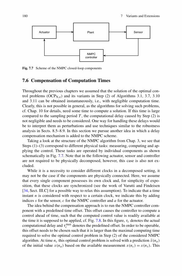
180 7 Variants and Extensions
Fig. 7.7 Scheme of the NMPC closed-loop components
7.6 Compensation of Computation Times
Throughout the previous chapters we assumed that the solution of the optimal con-trol problems (OCPN,e) and its variants in Step (2) of Algorithms 3.1, 3.7, 3.10and 3.11 can be obtained instantaneously, i.e., with negligible computation time.Clearly, this is not possible in general, as the algorithms for solving such problems,cf. Chap. 10 for details, need some time to compute a solution. If this time is largecompared to the sampling period T , the computational delay caused by Step (2) isnot negligible and needs to be considered. One way for handling these delays wouldbe to interpret them as perturbations and use techniques similar to the robustnessanalysis in Sects. 8.5–8.9. In this section we pursue another idea in which a delaycompensation mechanism is added to the NMPC scheme.
Taking a look at the structure of the NMPC algorithm from Chap. 3, we see thatSteps (1)–(3) correspond to different physical tasks: measuring, computing and ap-plying the control. These tasks are operated by individual components as shownschematically in Fig. 7.7. Note that in the following actuator, sensor and controllerare not required to be physically decomposed, however, this case is also not ex-cluded.
While it is a necessity to consider different clocks in a decomposed setting, itmay not be the case if the components are physically connected. Here, we assumethat every single component possesses its own clock and, for simplicity of expo-sition, that these clocks are synchronized (see the work of Varutti and Findeisen[34, Sect. III.C] for a possible way to relax this assumption). To indicate that a timeinstant n is considered with respect to a certain clock, we indicate this by addingindices s for the sensor, c for the NMPC controller and a for the actuator.
The idea behind the compensation approach is to run the NMPC controller com-ponent with a predefined time offset. This offset causes the controller to compute acontrol ahead of time, such that the computed control value is readily available atthe time it is supposed to be applied, cf. Fig. 7.8. In this figure, τc denotes the actualcomputational delay and τmax
c denotes the predefined offset. In order to be operable,this offset needs to be chosen such that it is larger than the maximal computing timerequired to solve the optimal control problem in Step (2) of the considered NMPCalgorithm. At time nc this optimal control problem is solved with a prediction x(na)
of the initial value x(na) based on the available measurement x(nc) = x(ns). This
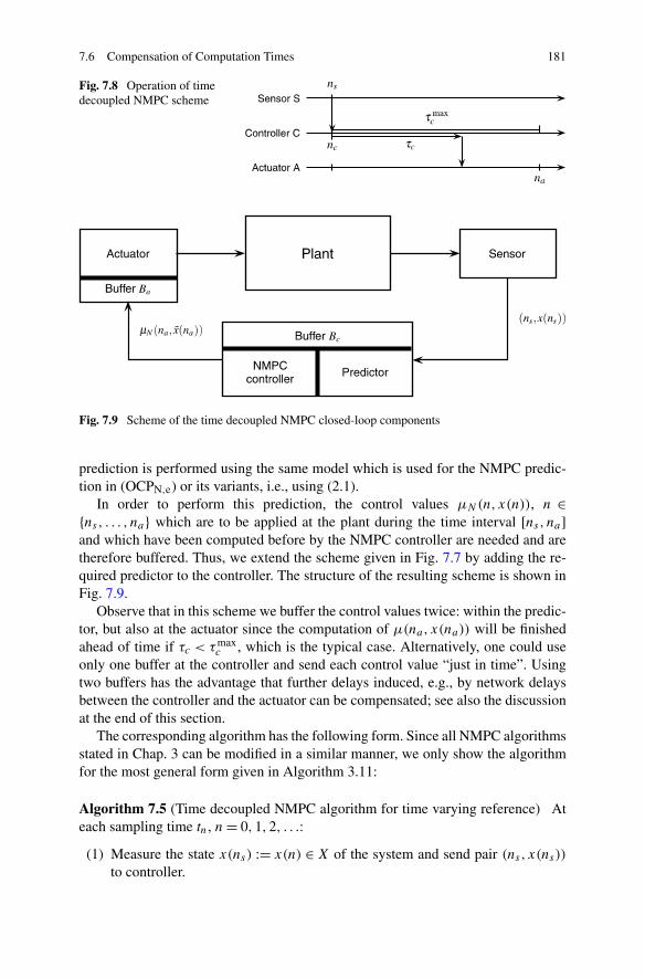
7.6 Compensation of Computation Times 181
Fig. 7.8 Operation of timedecoupled NMPC scheme
Fig. 7.9 Scheme of the time decoupled NMPC closed-loop components
prediction is performed using the same model which is used for the NMPC predic-tion in (OCPN,e) or its variants, i.e., using (2.1).
In order to perform this prediction, the control values μN(n,x(n)), n ∈{ns, . . . , na} which are to be applied at the plant during the time interval [ns, na]and which have been computed before by the NMPC controller are needed and aretherefore buffered. Thus, we extend the scheme given in Fig. 7.7 by adding the re-quired predictor to the controller. The structure of the resulting scheme is shown inFig. 7.9.
Observe that in this scheme we buffer the control values twice: within the predic-tor, but also at the actuator since the computation of μ(na, x(na)) will be finishedahead of time if τc < τmax
c , which is the typical case. Alternatively, one could useonly one buffer at the controller and send each control value “just in time”. Usingtwo buffers has the advantage that further delays induced, e.g., by network delaysbetween the controller and the actuator can be compensated; see also the discussionat the end of this section.
The corresponding algorithm has the following form. Since all NMPC algorithmsstated in Chap. 3 can be modified in a similar manner, we only show the algorithmfor the most general form given in Algorithm 3.11:
Algorithm 7.5 (Time decoupled NMPC algorithm for time varying reference) Ateach sampling time tn, n = 0,1,2, . . .:
(1) Measure the state x(ns) := x(n) ∈ X of the system and send pair (ns, x(ns))
to controller.

182 7 Variants and Extensions
(2a) Delete pair (nc − 1,μN(nc − 1, x(nc − 1))) from buffer Bc and compute thepredicted state x(nc + τmax
c ) from the measured state x(nc).(2b) Set n := nc + τmax
c , x0 = x(n) and solve the optimal control problem
minimize JN
(n, x0, u(·)) :=
N−1∑
k=0
ωN−k�(n+k, xu(k, x0), u(k)
)
+ F(n + N,xu(N,x0)
)
with respect to u(·) ∈ UNX0
(n, x0), subject to
xu(0, x0) = x0, xu(k + 1, x0) = f(xu(k, x0), u(k)
)
(OCPnN,e)
and denote the obtained optimal control sequence by u�(·) ∈ UNX0
(n, x0).(2c) Add pair (n,μN(n, x(n))) := (n, u�(0)) to Buffer Bc and send it to actuator.(3a) Delete pair (na − τmax
c − 1,μN(na − τmaxc − 1, x(na − τmax
c − 1))) and addreceived pair (na,μN(na, x(na))) to buffer Ba .
(3b) Use μN(na − τmaxc , x(na − τmax
c )) in the next sampling period.
At a first glance, writing this algorithm using three different clocks and sendingtime stamped information in Steps (1) and (2c) may be considered as overly compli-cated, given that ns in Step (1) is always equal to nc in Step (2a) and nc in Step (2c)always equals na in Step (3a). However, this way of writing the algorithm allows usto easily separate the components—sensor, predictor/controller and actuator—of theNMPC scheme and to assume that the “sending” in Steps (1) and (2c) is performedvia a digital network. Then, we can assign Step (1) to the sensor, Steps (2a)–(2c) tothe controller and Steps (3a) and (3b) to the actuator. Assuming that all transmis-sions between the components can be done with negligible delay, we can run thesethree steps as separate algorithms in parallel. Denoting the real time by n, the re-sulting scheduling structure is sketched in Fig. 7.10 for τmax
c = 2. For comparison,the structure of the NMPC Algorithm 3.11 without prediction is indicated by thedashed lines.
Since the algorithm is already applicable to work in parallel, it can be extended toa more complex networked control context in which transmission delays and packetloss may occur. To this end, such delays have to be considered in the predictionand an appropriate error handling must be added for handling dropouts; see, e.g.,the paper by Grüne, Pannek and Worthmann [19]. In the presence of transmissiondelays and dropouts, we cannot expect that all control values are actually availableat the actuator when they are supposed to be applied. Using NMPC, this can becompensated easily using the multistep feedback concept and the respective stabilityresults from Sect. 7.4 as presented by Grüne et al. in [18].
Besides [19], which forms the basis for the presentation in this section, modelbased prediction for compensating computational delay in NMPC schemes has beenconsidered earlier, e.g., in the works of Chen, Ballance and O’Reilly [4] and Find-eisen and Allgöwer [10]. Note that the use of the nominal model (2.1) for predicting

7.7 Online Measurement of α 183
Fig. 7.10 Comparison of scheduling structure between NMPC Algorithms 3.11 (dashed lines)and 7.5 (solid lines) with τmax
c = 2T
future states may lead to wrong predictions in case of model uncertainties, distur-bances etc. In this case, the predicted state x(n) may differ from the actual statex(na) at time na = n and hence (OCPN,e) is solved with a wrong initial value. Inthe paper of Zavala and Biegler [35] a method for correcting this mismatch basedon NLP sensitivity techniques is presented, cf. also Sect. 10.5.
7.7 Online Measurement of α
In the analysis of NMPC schemes without stabilizing terminal constraints inChap. 6, one of the central aims was to establish conditions to rigorously guaranteethe existence of α ∈ (0,1] such that the inequality
VN(n, x) ≥ α�(n,x,μN(n, x)
) + VN
(n + 1, f
(x,μN(n, x)
))(5.1)
holds for all x ∈ X and n ∈ N0. While Theorem 6.14 and Proposition 6.17 providecomputational methods for estimating α from the problem data, the assumptionsneeded for these computations—in particular Assumption 6.4—may be difficult tocheck.
In this section we present methods from Grüne and Pannek [15] and Pannek [29]which allow for the online computation or estimation of α along simulated NMPCclosed-loop trajectories. There are several motivations for proceeding this way. First,as already mentioned, it may be difficult to check the assumptions needed for thecomputation of α using Theorem 6.14 or Proposition 6.17. Although a simulationbased computation of α for a selection of closed-loop trajectories cannot rigorouslyguarantee stability and performance for all possible closed-loop trajectories, it maystill give valuable insight into the performance of the controller. In particular, theinformation obtained from such simulations may be very useful in order to tunethe controller parameters, in particular the optimization horizon N and the runningcost �.
Second, requiring (5.1) to hold for all x ∈ X may result in a rather conservativeestimate for α. As we will see in Proposition 7.6, below, for assessing the perfor-

184 7 Variants and Extensions
mance of the controller along one closed-loop trajectory it is sufficient that (5.1)holds only for those points x ∈ X which are actually visited by this trajectory.
Finally, the knowledge of α may be used for an online adaptation of the opti-mization horizon N ; some ideas in this direction are described in the subsequentSect. 7.8.
Our first result shows that for assessing stability and performance of the NMPCcontroller along one specific closed-loop trajectory it is sufficient to find α such that(5.1) holds for the points actually visited by this trajectory.
Proposition 7.6 Consider the feedback law μN : N0 × X → U computed fromAlgorithm 3.7 and the closed-loop trajectory x(·) = xμN
(·) of (3.9) with initial valuex(0) ∈ X at initial time 0. If the optimal value function VN : N0 × X → R
+0 satisfies
VN
(n,x(n)
) ≥ VN
(n + 1, x(n + 1)
) + α�(n,x(n),μN
(n,x(n)
))(7.10)
for some α ∈ (0,1] and all n ∈ N0, then
αV∞(n,x(n)
) ≤ αJ∞(n,x(n),μN
) ≤ VN
(n,x(n)
) ≤ V∞(n,x(n)
)(7.11)
holds for all n ∈ N0.If, in addition, there exist α1, α2, α3 ∈ K∞ such that (5.2) holds for all (n, x) ∈
N0 × X with n ∈ N0 and x = x(n), then there exists β ∈ K L which only depends onα1, α2, α3 and α such that the inequality
∣∣x(n)∣∣xref(n)
≤ β(∣∣x(0)
∣∣xref(0)
, n)
holds for all n ∈ N0, i.e., x behaves like a trajectory of an asymptotically stablesystem.
Proof The proof of (7.11) is similar to the proof of Theorem 4.11.The existence of β follows with the same construction as in the proof of Theo-
rem 2.19, observing that the definition of β in this proof only depends on α1, α2 andαV = αα3 and not on the specific form of V = VN . �
Proposition 7.6 gives us a way to compute α from the data available at runtimeand guarantees the performance estimate (7.11) as well as—under the additionalassumption that (5.2) holds—asymptotic stability-like behavior for the consideredclosed-loop trajectory if α > 0. Moreover, under this additional assumption (7.10)immediately implies that VN strictly decreases along the trajectory, i.e., it behaveslike a Lyapunov function.
Since the values of α for which (5.1) holds for all x ∈ X and for which (7.10)holds along a specific trajectory xμN
will be different in general, we introduce thefollowing definition.
Definition 7.7
(1) We call α := max{α | (5.1) holds for all x ∈ X} the global suboptimality degree.(2) For fixed x ∈ X the maximal value of α satisfying (5.1) for this x is called local
suboptimality degree in x.

7.7 Online Measurement of α 185
(3) Given a closed-loop trajectory xμN(·) of (3.9) with initial time 0 we call
α := max{α | (7.10) holds for all n ∈ N0 with x(·) = xμN(·)} the closed-loop
suboptimality degree along xμN(·).
An algorithm to evaluate α from (7.10) can easily be obtained and integrated intoAlgorithm 3.7:
Algorithm 7.8 (NMPC algorithm for time varying reference xref with a posteriorisuboptimality estimate) Set α = 1. At each sampling time tn, n = 0,1,2, . . . :
(1) Measure the state x(n) ∈ X of the system.(2) Set x0 = x(n) and solve the optimal control problem
minimize JN
(n,x0, u(·)) :=
N−1∑
k=0
�(n+k, xu(k, x0), u(k)
)
with respect to u(·) ∈ UN(x0), subject to
xu(0, x0) = x0, xu(k + 1, x0) = f(xu(k, x0), u(k)
)
(OCPnN)
and denote the obtained optimal control sequence by u�(·) ∈ UN(x0).
(3) Define the NMPC-feedback value μN(n,x(n)) := u�(0) ∈ U and use this con-trol value in the next sampling period.
(4) If n ≥ 1 compute α via
αl = VN(n − 1, x(n − 1)) − VN(n, x(n))
�(n − 1, x(n − 1),μN(n − 1, x(n − 1))),
α = min{α,αl}.
Proposition 7.6 and Algorithm 7.8 are easily extended to the multistep NMPCcase described in Sect. 7.4. In this case, (7.10) is replaced by
VN
(n,x(n)
) ≥ VN
(n + m + 1, x(n + m + 1)
)
+ α
m∑
k=0
�(n + k, xu
(k, x(n)
), u�
(k, x(n)
))
and the definition of αl in Step (4) is changed, accordingly.Note that in Step (4) of Algorithm 7.8, the computation of αl does not provide
the value of α in (7.10) for the current time instant n but for n − 1. This is whywe call α from Algorithm 7.8 an a posteriori estimate. The distinction betweenthe current value of αl and α in Step (4) is required in order to be consistent withProposition 7.6 since αl corresponds to the local suboptimality degree in x(n − 1)
while the suboptimality degree according to Proposition 7.6 is the minimum overall αl along the closed loop.
While Algorithm 7.8 is perfectly suited in order to evaluate the performance ofan NMPC controller via numerical simulations, its a posteriori nature is not suitableif we want to use the estimated α in order to adjust the optimization horizon N . For

186 7 Variants and Extensions
instance, if we detect that at some time n the value of α in (7.10) is too small—oreven negative—then we may want to increase N in order to increase α (see Sect. 7.8for more details on such procedures). However, in Algorithm 7.8 the value of α in(7.10) only becomes available at time n + 1, which is too late in order to adjust N .
A simple remedy for this problem is to solve at time n a second optimal controlproblem (OCPn
N) with initial value xu(1, x(n)) and initial time n := n+1. However,since solving the problem (OCPn
N) is the computationally most expensive part of theNMPC algorithm, this solution would be rather inefficient.
In order to obtain an a priori estimate with reduced additional computing costs,a few more insights into the local NMPC problem structure are required. The maintool we are going to use is the following lemma.
Lemma 7.9 Consider the feedback law μN : N0 × X → U computed from Algo-rithm 3.7 and the closed-loop trajectory x(·) = xμN
(·) of (3.9) with initial valuex(0) = x0 ∈ X at initial time 0. If
VN
(n + 1, x(n + 1)
) − VN−1(n + 1, x(n + 1)
)
≤ (1 − α)�(n,x(n),μN
(n,x(n)
))(7.12)
holds for some α ∈ [0,1] and some n ∈ N0, then (7.11) holds for this n.
Proof Using the dynamic programming principle (3.16) with K = 1 we obtain
VN
(n,x(n)
) = �(n,x(n),μN
(n,x(n)
)) + VN−1(n + 1, x(n + 1)
)
≥ �(n,x(n),μN
(n,x(n)
)) + VN
(n + 1, x(n + 1)
)
− (1 − α)�(n,x(n),μN
(n,x(n)
))
= VN
(n + 1, x(n + 1)
) + α�(n,x(n),μN
(n,x(n)
)).
Hence, (7.10) holds and Proposition 7.6 guarantees the assertion. �
Now, we would not gain much if we tried to compute α using (7.12) directly,since we would again need the future information VN(n + 1, x(n + 1)), i.e., thesolution of another optimal control problem (in contrast to that VN−1(n + 1, x(n +1)) is readily available at time n since by the dynamic programming principle it canbe computed from VN(n, x(n)) and �(x(n),μN(x(n)))). There is, however, a wayto reduce the size of the additional optimal control problem that needs to be solved.To this end, we introduce the following assumption which will later be checkednumerically in our algorithm.
Assumption 7.10 For given N , N0 ∈ N, N ≥ N0 ≥ 2, there exists a constant γ > 0such that for the optimal open-loop solution xu�(·, x(n)) of (OCPn
N) in Algorithm 3.7the inequalities
VN0(n + N − N0, xu�(N − N0, x(n)))
γ + 1

7.7 Online Measurement of α 187
≤ maxj=N−N0,...,N−2
�(n + j, xu
(n + j, x(n)
),μN−j−1
(n + j, xu�
(j, x(n)
))),
Vk(n + N − k, xu�(N − k, x(n)))
γ + 1
≤ �(n + N − k, xu�
(N − k, x(n)
),μk
(n + N − k, xu�
(N − k, x(n)
)))
hold for all k ∈ {N0 + 1, . . . ,N} and all n ∈ N0.
Note that computing γ for which this assumption holds requires only the com-putation of μj for j = 1, . . . ,N0 − 1 in the first inequality, since μk in the secondinequality can be obtained from u� via (3.23). This corresponds to solving N0 − 2additional optimal control problems which may look like a step backward, but sincethese optimal control problems are defined on a significantly smaller horizon, thecomputing costs are actually reduced. In fact, in the special case that � does notdepend on u, no additional computations have to be performed, at all. In this as-sumption, the value N0 is a design parameter which affects the computational effortfor checking Assumption 7.10 as well as the accuracy of the estimate for α obtainedfrom this assumption.
Under Assumption 7.10 we can relate the minimal values of two optimal controlproblems with different horizon lengths.
Proposition 7.11 Suppose that Assumption 7.10 holds for N ≥ N0 ≥ 2. Then
(γ + 1)N−N0
(γ + 1)N−N0 + γ N−N0+1VN
(n,x(n)
) ≤ VN−1(n,x(n)
)
holds for all n ∈ N0.
Proof In the following we use the abbreviation xu(j) := xu(j, x(n)), j = 0, . . . ,N ,since all our calculations use the open-loop trajectory with fixed initial value x(n).
Set n := N −k. Using the principle of optimality and Assumption 7.10 we obtain
Vk−1(n + n + 1, f
(xu(n),μk
(n + n, xu(n)
)))
≤ γ �(n + n, xu(n),μk
(n + n, xu(n)
))(7.13)
for all k ∈ {N0 + 1, . . . ,N} and all n ∈ N0.
We abbreviate ηk = (γ+1)k−N0
(γ+1)k−N0+γ k−N0+1 and prove the main assertion
ηkVk(n + n, xu(n)) ≤ Vk−1(n + n, xu(n)) by induction over k = N0, . . . ,N . Bychoosingxu(0) = x(n) with n being arbitrary but fixed we obtain
VN0
(n + N − N0, xu(N − N0)
)
≤ (γ + 1) maxj=2,...,N0
�(n + N − j, xu(N − j),μj−1
(n + N − j, xu(N − j)
))
≤ (γ + 1)
N0∑
j=2
�(n + N − j, xu(N − j),μj−1
(n + N − j, xu(N − j)
))

188 7 Variants and Extensions
= 1
ηN0
VN0−1(n + N − N0, xu(N − N0)
).
For the induction step k → k +1 the following holds, using (7.13) and the inductionassumption:
Vk
(n + n, xu(n)
)
= Vk−1(n + n + 1, f
(xu(n),μk
(n + n, xu(n)
)))
+ �(n + n, xu(n),μk
(n + n, xu(n)
))
≥ ηk
(1 + 1 − ηk
γ + ηk
)Vk
(n + n + 1, f
(xu(n),μk
(n + n, xu(n)
)))
+(
1 − γ1 − ηk
γ + ηk
)�(n + n, xu(n),μk
(n + n, xu(n)
))
= ηk
γ + 1
γ + ηk
(Vk
(n + n + 1, f
(xu(n),μk
(n + n, xu(n)
)))
+ �(n + n, xu(n),μk
(n + n, xu(n)
)))
using the dynamic programming principle (3.16) with K = 1 in the last step. Hence,we obtain Vk(n + n, xu(n)) ≥ ηk
γ+1γ+ηk
Vk+1(n + n, xu(n)) with
ηk
γ + 1
γ + ηk
= (γ + 1)k−2
(γ + 1)k−2 + γ k−1
γ + 1
γ + (γ+1)k−2
(γ+1)k−2+γ k−1
= (γ + 1)k−1
(γ + 1)k−1 + γ k= ηk+1.
If we choose k = N then we get n = 0. Inserting this into our induction result wecan use xu(0) = xu(0, x(n)) = x(n) and the assertion holds. �
Finally, we can now use Proposition 7.11 within the NMPC closed loop. This al-lows us to verify Condition (7.12) and to estimate α directly from Assumption 7.10.
Theorem 7.12 Consider γ > 0 and N , N0 ∈ N, N ≥ N0 such that (γ + 1)N−N0 >
γ N−N0+2 holds. If Assumption 7.10 is fulfilled for these γ , N and N0, then theestimate (7.11) holds for all n ∈ N0 where
α := (γ + 1)N−N0 − γ N−N0+2
(γ + 1)N−N0. (7.14)
Proof From Proposition 7.11 we know
VN
(n,x(n)
) − VN−1(n,x(n)
) ≤ γ N−N0+1
(γ + 1)N−N0VN−1
(n,x(n)
).
Setting j = n − 1, we can reformulate this and obtain
VN
(j + 1, x(j + 1)
) − VN−1(j + 1, x(j + 1)
)
≤ γ N−N0+1
(γ + 1)N−N0VN−1
(j + 1, f
(xu
(0, x(j)
),μN
(j, xu
(0, x(j)
))))

7.7 Online Measurement of α 189
using the dynamics of the optimal open-loop solution. Now, we can use (7.13) withk = N and get
VN
(j + 1, x(j + 1)
) − VN−1(j + 1, x(j + 1)
)
≤ γ N−N0+2
(γ + 1)N−N0�(j, x(j),μN
(j, x(j)
)).
Hence, the assumptions of Lemma 7.9 are fulfilled with
α = 1 − γ N−N0+2
(γ + 1)N−N0= (γ + 1)N−N0 − γ N−N0+2
(γ + 1)N−N0
and the assertion follows. �
Similar to Proposition 7.6, the required values of γ and α are easily computableand allow us to extend Algorithm 3.7 in a similar manner as we did in Algorithm 7.8.
Algorithm 7.13 (NMPC algorithm for time varying reference xref with a priori sub-optimality estimate) Set α = 1. At each sampling time tn, n = 0,1,2, . . . :
(1) Measure the state x(n) ∈ X of the system.(2) Set x0 = x(n) and solve the optimal control problem
minimize JN
(n,x0, u(·)) :=
N−1∑
k=0
�(n+k, xu(k, x0), u(k)
)
with respect to u(·) ∈ UN(x0), subject to
xu(0, x0) = x0, xu(k + 1, x0) = f(xu(k, x0), u(k)
)
(OCPnN)
and denote the obtained optimal control sequence by u�(·) ∈ UN(x0).
(3) Define the NMPC-feedback value μN(n,x(n)) := u�(0) ∈ U and use this con-trol value in the next sampling period.
(4) Compute α via
Find the minimal γ which satisfies the inequalities
in Assumption 7.10 for the current n and set
α = min
{α,
(γ + 1)N−N0 − γ N−N0+2
(γ + 1)N−N0
}.
Note that checking the additional condition (γ + 1)N−N0 > γ N−N0+2 from The-orem 7.12 is unnecessary, since a violation would lead to a negative α in which caseasymptotic stability cannot be guaranteed by means of Theorem 7.12, anyway.
Similar to Proposition 7.6, the results from Theorem 7.12 are easily carried overto the multistep NMPC case described in Sect. 7.4 by extending Assumption 7.10.
Example 7.14 To illustrate these results, we consider the inverted pendulum on acart problem from Example 2.10 with parameters g = 9.81, l = 10 and kR = kL =

190 7 Variants and Extensions
Fig. 7.11 Vector field and cost function
0.01 and control constraint set U = [−15,15]. Our aim is to stabilize one of theupright positions x ∈ S := {((k + 1)π,0,0,0)� | k ∈ 2Z}. For this example we willprovide online measurements of α using Algorithm 7.8 for one fixed initial valueand varying terminal weights ω, cf. Sect. 7.2, and control horizons, cf. Sect. 7.4. Fora comparison of Algorithms 7.8 and 7.13 we refer to [15] and [29].
In order to obtain a suitable cost function, we follow the guidelines from Sect. 6.6and construct a cost function for which—at least in the first two components—the overshoot of � along a typical stable trajectory becomes small. To this end, wehave used the geometry of the vector field of the first two differential equationsrepresenting the pendulum, see Fig. 7.11(a), and shaped the cost function such thatit exhibits local maxima at the downward equilibria and “valleys” along the stablemanifolds of the upright equilibria to be stabilized. The resulting cost function � isof the integral type (3.4) with
L(x,u) := 10−4u2 + (3.51 sin(x1 − π)2 + 4.82 sin(x1 − π)x2
+ 2.31x22 + 0.1
((1 − cos(x1 − π)
) · (1 + cos(x2)2))2
+ 0.01x23 + 0.1x2
4
)2,
cf. Fig. 7.11(b). Using the terminal weights from Sect. 7.2, the cost functional be-comes
JN(x0, u) =N−2∑
i=0
�(x(i), u(i)
) + ω�(x(N − 1), u(N − 1)
).
This way of adjusting the cost function to the dynamics allows us to considerablyreduce the length of the optimization horizon for obtaining stability in the NMPCscheme without stabilizing terminal constraints compared to simpler choices of �.

7.8 Adaptive Optimization Horizon 191
Fig. 7.12 Computed value for αω70,m for the nonlinear inverted pendulum example 2.10 with con-
trol horizons m ∈ {1, . . . ,20} and terminal weights ω ∈ {1, . . . ,10}
However, for the initial value x0 = (2π +1.5,0,0,0) and sampling period T = 0.05,which have been used in the subsequent computations, we still need a rather largeoptimization horizon of N = 70 to obtain stability of the closed loop.
Since the cost function is 2π -periodic it does not penalize the distance to a spe-cific equilibrium in S ; rather, it penalizes the distance to the whole set. For a bettercomparison of the solutions for different parameters we want to force the algorithmto stabilize one specific upright position in S . To this end, we add box-constraintsto X limiting the x1-component to the interval [−π + 0.01,3π − 0.01]. The toler-ances of the optimization routine and the differential equation solver are set to 10−6
and 10−7, respectively. The NMPC closed-loop trajectories displayed in Fig. 7.12are simulated for terminal weights ω = 1, . . . ,10, cf. Sect. 7.2, and control horizonsm = 1, . . . ,10, cf. Sect. 7.4. The resulting α-values from Algorithm 7.8, denoted byαω
N,m, are shown in Fig. 7.12.Note that for ω = 1 the α values are negative for control horizons m = 1, . . . ,4.
Still, larger control horizons exhibit a positive α value such that stability is guaran-teed. This is in accordance with the theoretical results from Sect. 7.4, even thoughthese simulation based results do not share the monotonicity of the theoreticalbounds from Fig. 7.3. Additionally, an increase of α can be observed for all con-trol horizons m if ω is increased. This confirms the stabilizing effect of terminalcosts shown theoretically in Sect. 7.2; cf. Fig. 7.1.
Summarizing, these results show that the online measurement of α yields valu-able insights into the performance analysis of NMPC schemes without terminalconstraints and thus nicely complements the theoretical results from Chap. 6 andSects. 7.2 and 7.4.
7.8 Adaptive Optimization Horizon
In the previous Sect. 7.7 we have shown how the suboptimality degree α can becomputed at runtime of the NMPC scheme without stabilizing terminal constraints.

192 7 Variants and Extensions
If the horizon length N is not chosen adequately, then it is likely that during runtimea value α < 0 is obtained. In this case, stability of the closed loop cannot be guaran-teed by Proposition 7.6 or Theorem 7.12. However, the ability to compute α for eachpoint x(n) on the closed-loop trajectory using the techniques from Sect. 7.7 natu-rally leads to the idea of adapting the optimization horizon N at each time n suchthat stability and desired performance can be guaranteed. In this section, we willshow some algorithms for this purpose, taken from Pannek [29]. Here we restrictourselves to the basic idea and refer to [29] for more sophisticated approaches.
The fundamental idea of such an adaptive algorithm is rather simple: introducinga stability and suboptimality threshold α > 0, at each sampling instant n we prolongthe optimization horizon if α for the current horizon is smaller than α. If α > α
holds, then we may reduce N in order to save computational time. This leads to thefollowing algorithm.
Algorithm 7.15 (Adaptive horizon NMPC algorithm for time varying reference)Set N0 > 0 and α > 0. At each sampling time tn, n = 0,1,2, . . . :
(1) Measure the state x(n) ∈ X of the system and set α = 0.(2) While α > α
(a) Set x0 = x(n), N = Nn and solve the optimal control problem
minimize JN
(n,x0, u(·)) :=
N−1∑
k=0
�(n+k, xu(k, x0), u(k)
)
with respect to u(·) ∈ UN(x0), subject to
xu(0, x0) = x0, xu(k + 1, x0) = f(xu(k, x0), u(k)
).
(OCPnN)
Denote the obtained optimal control sequence by u�(·) ∈ UN(x0).
(b) Compute α via Proposition 7.6 or Theorem 7.12.(c) If α > α call reducing strategy for Nn, else call increasing strategy for Nn;
obtain u�(·) for the new N = Nn and an initial guess for Nn+1.(3) Define the NMPC-feedback value μN(n,x(n)) := u�(0) ∈ U and use this con-
trol value in the next sampling period.
Here, the initial guess Nn+1 in Step (2c) will typically be Nn+1 = Nn, however,as we will see below, in the case of reducing Nn the choice Nn+1 = Nn − 1 is moreefficient, cf. the discussion after Proposition 7.18.
If this algorithm is successful in ensuring α ≥ α for each n, then the assumptionsof Proposition 7.6 or Theorem 7.12 are satisfied. However, these results require theoptimization horizon N to be fixed and hence do not apply to Algorithm 7.15 inwhich Nn changes with time.
To cope with this issue, we generalize Proposition 7.6 to varying optimizationhorizons. To this end, for each x ∈ X and N ∈ N we denote the maximal α from(7.10) by α(N). We then introduce the following assumption, which guarantees thatfor any horizon N satisfying α(N) ≥ α the controller shows a bounded guaranteedperformance if the horizon length is increased.

7.8 Adaptive Optimization Horizon 193
Assumption 7.16 Given n ∈ N0, x ∈ X, N < ∞ and a value α ∈ (0,1) withα(N) ≥ α, we assume that there exist constants Cl,Cα > 0 such that the inequalities
Cl�(n,x,μN(n, x)
)
≤ �(n,x,μN (n, x)
)VN (n, x) − VN (n + 1, f (x,μN(n, x)))
VN (n, x) − VN (n + 1, f (x,μN (n, x))), (7.15)
Cαα(N) ≤ α(N) (7.16)
hold for all N ≥ N .
The reason for Assumption 7.16 is that it is possible that the performance of thecontroller μN may not improve monotonically as N increases; see Di Palma andMagni [6]. Consequently, we cannot expect α(N) ≥ α(N) for N > N . Still, we needto ensure that α(N) does not become too small compared to α(N), in particular,α(N) should not drop below zero if the horizon length is increased; this is ensuredby (7.16). Furthermore, we need an estimate for the dependence of �(n, x,μN(n, x))
on N which is given by (7.15). Unfortunately, for both inequalities so far we werenot able to provide sufficient conditions in terms of the problem data, like, e.g., acontrollability condition similar to Assumption 6.4. Still, numerical evaluation forseveral examples showed that these inequalities are satisfied and that Cl and Cα
attain reasonable values.Using Assumption 7.16, we obtain a stability and performance estimate of the
closed loop in the context of changing horizon lengths similar to Proposition 7.6.Since the closed-loop control resulting from Algorithm 7.15 now depends on a se-quence of horizons (Nn)n∈N0 we obtain a sequence of control laws (μNn
)n∈N0 . Theclosed-loop trajectory generated by this algorithm is then given by
x(n + 1) = f(x(n),μNn
(n,x(n)
)). (7.17)
Theorem 7.17 Consider the sequence of feedback laws (μNn) computed from Al-gorithm 7.15 and the corresponding closed-loop trajectory x(·) from (7.17). Assumethat for optimal value functions VNn : N0 × X → R
+0 of (OCPn
N) with N = Nn theinequality
VNn
(n,x(n)
) ≥ VNn
(n + 1, x(n + 1)
) + α�(n,x(n),μNn
(n,x(n)
))(7.18)
holds for all n ∈ N0 and that Assumption 7.16 is satisfied for all triplets (n, x,N) =(n, x(n),Nn), n ∈ N0, with constants C
(n)l , C
(n)α . Then
αCV∞(n,x(n)
) ≤ αCJ∞(n,x(n),μ(Nn)
) ≤ VN�
(n,x(n)
) ≤ V∞(n,x(n)
)(7.19)
holds for all n ∈ N0 where αC := mini∈N≥nC
(i)α C
(i)l α.
Proof Given (i, x(i),Ni) for some i ∈ N0, Assumption 7.16 for (n, x,N) =(i, x(i),Ni) guarantees α(Ni) ≤ α(N)/C
(i)α for N ≥ Ni . Choosing N = N�, we ob-
tain α ≤ α(Ni) ≤ α(N�)/C(i)α using the relaxed Lyapunov Inequality (7.18). Multi-
plying by the stage cost �(i, x(i),μNi(i, x(i))), we can conclude

194 7 Variants and Extensions
α�(i, x(i),μNi
(i, x(i)
))
≤ α(N�)
C(i)α
�(i, x(i),μNi
(i, x(i)
))
= VN�(i, x(i)) − VN�(i + 1, f (x(i),μN�(i, x(i))))
C(i)α �(i, x(i),μN�(i, x(i)))
�(i, x(i),μNi
(i, x(i)
))
≤ VN�(i, x(i)) − VN�(i + 1, f (x(i),μNi(i, x(i))))
C(i)α C
(i)l
using (7.18) and (7.15). In particular, the latter condition allows us to use an identicaltelescope sum argument as in the proof of Proposition 7.6 since it relates the closed-loop varying optimization horizon to a fixed one. Hence, summing the running costsalong the closed-loop trajectory reveals
αC
K∑
i=n
�(i, x(i),μNi
(i, x(i)
)) ≤ VN�
(n,x(n)
) − VN�
(K + 1, x(K + 1)
)
where we defined αC := mini∈[n,...,K] C(i)α C
(i)l α. Since VN�(K + 1, x(K + 1)) ≥ 0
holds, we can neglect it in the last inequality. Taking K to infinity yields
αCVμ(Ni )∞
(n,x(n)
) = αC limK→∞
K∑
i=n
�(i, x(i),μNi
(i, x(i)
)) ≤ VN�
(n,x(n)
).
Since the first and the last inequality of (7.19) hold by definition of VN and V∞, theassertion follows. �
If the conditions of this theorem hold, then stability-like behavior of the closedloop can be obtained analogously to Proposition 7.6.
Having shown the analytical background, we now present adaptation strategieswhich can be used for increasing or reducing the optimization horizon N in Step (2c)of Algorithm 7.15. For simplicity of exposition, we restrict ourselves to two simplestrategies and consider a posteriori estimates based variants only. Despite their sim-plicity, these methods have shown to be reliable and fast in numerical simulations.A more detailed analysis, further methods and comparisons can be found in [29].The following proposition yields the basis for a strategy for reducing Nn.
Proposition 7.18 Consider the optimal control problem (OCPnN) with initial value
x0 = x(n), Nn ∈ N, and denote the optimal control sequence by u�. For fixed α ∈(0,1), suppose there exists an integer i ∈ N0, 0 ≤ i < N such that
VNn−i
(n + i + 1, xu�
(i + 1, x(n)
))
+ α�(n + i, xu�
(i, x(n)
),μNn−i
(n + i, xu�
(i, x(n)
)))
≤ VNn−i
(n + i, xu�
(i, x(n)
))(7.20)
holds for all 0 ≤ i ≤ i. Then, setting Nn+i = Nn − i and μNn+i(n + i, x(n + i)) =
u�(i) for 0 ≤ i ≤ i − 1, Inequality (7.18) holds for n = n, . . . , n + i − 1.

7.8 Adaptive Optimization Horizon 195
Proof The proof follows immediately from the fact that for μNn+i(n + i, x(n +
i)) = u�(i) the closed-loop trajectory (7.17) satisfies x(n+ i) = xu�(i, x(n)). Hence,(7.18) follows from (7.20). �
Observe that Proposition 7.18 is quite similar to the results from Sect. 7.4, sinceμNn+i
(n + i, x(n + i)) as defined in this theorem coincides with the multistep feed-back law from Sect. 7.4. Thus, Proposition 7.18 guarantees that if i > 1, then themultistep NMPC feedback from Sect. 7.4 can be applied with m = i steps such thatthe suboptimality threshold α can be guaranteed. With the choice Nn+i = Nn − i,due to the principle of optimality we obtain that the optimal control problems withinthe next i − 1 NMPC iterations are already solved since μNn+i
(n + i, x(n + i)) canbe obtained from the optimal control sequence u�(·) ∈ U
N(x(n)) computed at timen. This implies that the most efficient way for the reducing strategy in Step (2c) ofAlgorithm 7.15 is not to reduce Nn itself but rather to reduce the horizons Nn+i byi for the subsequent sampling instants n + 1, . . . , n + i, i.e., we choose the initialguess in Step (2c) as Nn+1 = Nn − 1. Still, if the a posteriori estimate is used, theevaluation of (7.20) requires the solution of an additional optimal control problemin each step in order to compute VNn−i (n + i + 1, xu�(i + 1, x(n))).
In contrast to this efficient and simple shortening strategy, it is quite difficultto obtain efficient methods for prolonging the optimization horizon N in Step (2c)of Algorithm 7.15. In order to understand why this is the case, we first introducethe basic idea behind any such prolongation strategy: at each sampling instant weiteratively increase the horizon Nn until (7.18) is satisfied and use this horizon forthe next NMPC step. In order to ensure that iteratively increasing Nn will eventuallylead to a horizon for which (7.18) holds, we make the following assumption.
Assumption 7.19 Given α ∈ (0,1), for all x0 ∈ X and all n ∈ N0 there exists afinite horizon length N = N(n,x0) ∈ N such that (7.18) holds with α(Nn) ≥ α forx(n) = x0 and Nn ≥ N .
Assumption 7.19 can be seen as a performance assumption which requires theexistence of a horizon length Nn such that the predefined threshold α can be sat-isfied. If no such horizon exists, no prolongation strategy can be designed whichcan guarantee closed-loop suboptimality degree α > α. Assumption 7.19 is, for in-stance, satisfied if the conditions of Theorem 6.21 hold.
The following proposition shows that under this assumption any iterative strategywhich increases the horizon will terminate after finitely many steps with a horizonlength N for which the desired local suboptimality degree holds.
Proposition 7.20 Consider the optimal control problem (OCPnN) with initial value
x0 = x(n) and Nn ∈ N. For fixed α ∈ (0,1) suppose that Assumption 7.19 holds.Then, any algorithm which iteratively increases the optimization horizon Nn andterminates if (7.18) holds will terminate in finite time with an optimization hori-zon Nn for which (7.18) holds. In particular, Theorem 7.17 is applicable providedAssumption 7.16 holds.
196 7 Variants and Extensions
Proof The proof follows immediately from Assumption 7.19. �
Unfortunately, if (7.18) does not hold it is in general difficult to assess by howmuch Nn should be increased such that (7.18) holds for the increased Nn. The mostsimple strategy of increasing Nn by one in each iteration shows satisfactory resultsin practice, however, in the worst case it requires us to check (7.18) N − Nn + 1times at each sampling instant. In contrast to the shortening strategy, the principleof optimality cannot be used here to establish a relation between the optimal con-trol problems for different Nn and, moreover, these problems may exhibit differentsolution structures which makes it a hard task to provide a suitable initial guess forthe optimization algorithm; see also Sect. 10.5.
In order to come up with more efficient strategies, different methods have beendeveloped [29] which utilize the structure of the suboptimality estimate itself todetermine by how much Nn should be increased. Compared to these methods, how-ever, the performance of the simple strategy of increasing Nn by one is still ac-ceptable. In the following example we illustrate the performance of this strategy forExample 2.11.
Example 7.21 For the ARP system (2.19)–(2.26) we have already analytically de-rived a continuous time tracking feedback in (2.28). However, this feedback law per-forms poorly under sampling, in particular, for the sampling period T = 0.2 whichwe consider here we obtain an unstable closed-loop sampled data system.
In order to obtain a sampled data feedback law which shows better performancewe use the digital redesign technique proposed by Nešic and Grüne in [27]: givena signal v(t) to track, we numerically simulate the continuous time controlled sys-tem in order to generate the output xref which in turn will be used as the refer-ence trajectory for an NMPC tracking problem. The advantage of proceeding thisway compared to the direct formulation of an NMPC tracking problem lies in thefact that—according to our numerical experience—the resulting NMPC problem ismuch easier to solve and in particular requires considerably smaller optimizationhorizons in order to obtain a stable NMPC closed loop.
Specifically, we consider the piecewise constant reference function
v(t) ={
10, t ∈ [0,5) ∪ [9,10),
0, t ∈ [5,9) ∪ [10,15)
for the x5-component of the trajectory of the system. In order to obtain short tran-sient times for the continuous time feedback, we set the design parameters ci in(2.28) to (c0, c1, c2, c3) = (10 000,3500,500,35). Then, we incorporate the result-ing trajectory displayed in Fig. 7.13 as reference xref(·) in the NMPC algorithm.Since our goal is to track the reference with the x5-component of the trajectory, weuse the simple quadratic cost function
J (x0, u) =N∑
j=0
∫ tj+1
tj
∣∣x5,u(t, x0) − x5,ref(t)∣∣dt

7.8 Adaptive Optimization Horizon 197
Fig. 7.13 Reference functionfor the continuous timefeedback (solid) and statetrajectory using thecontinuous time feedback(dashed). The latter will beused as reference functionwithin the NMPC algorithm
Fig. 7.14 Optimizationhorizons computed by theadaptive NMPCAlgorithm 7.15 for the ARPproblem using the a posterioriestimate (solid) and the apriori estimate (dashed)
within the adaptive horizon NMPC Algorithm 7.15. Moreover, we select the sam-pling period T = 0.2 and fix the initial value x(0) = (0,0,0,0,10,0,0,0) for boththe continuously and the sampled-data controlled system.
Using the a posteriori and a priori estimation techniques within the adaptiveNMPC Algorithm 7.15, we obtain the evolutions of horizons Nn along the closedloop for the suboptimality bound α = 0.1 as displayed in Fig. 7.14. Comparing thehorizons chosen by the a priori and the a posteriori estimates, one sees that the aposteriori algorithms yields smaller optimization horizons which makes the result-ing scheme computationally more efficient, however, at the expense that the evalua-tion of the a posteriori criterion itself is computationally more demanding; see alsoFig. 7.15, below.
It is also interesting to compare these horizons to the standard NMPC Algo-rithm 3.7 with fixed N which needs a horizon of N = 6 in order to guarantee α ≥ α
along the closed loop. Here, one observes that the required horizon Nn for the adap-tive NMPC approach is typically smaller than N = 6 for both the a posteriori andthe a priori estimate based variant. One also observes that the horizon is increasedat the jump points of the reference function v(·), which is the behavior one wouldexpect in a “critical” situation and nicely reflects the ability of the adaptive horizonalgorithm to adapt to the new situation.
Although the algorithm chooses to modify the horizon length throughout the runof the closed loop, one can barely see a difference between the resulting x5 trajecto-ries and the (dashed) reference trajectory given in Fig. 7.13. For this reason, we donot display the closed-loop solutions. Instead, we additionally plotted the computingtimes of the two adaptive NMPC variants in Fig. 7.15. Again, one can immediatelysee the spikes in the graph right at the points in which v(·) jumps. This figure alsoillustrates the disadvantage of the algorithm of having to solve multiple additionaloptimal control problems whenever N is increased, which clearly shows up in the

198 7 Variants and Extensions
Fig. 7.15 Computing timesof the adaptive NMPCAlgorithm 7.15 for the ARPproblem using the a posterioriestimate (solid) and the apriori estimate (dashed)
higher computation times at these points, in particular for the computationally moreexpensive a posteriori estimation.
While the adaptive optimization horizon algorithm produces good results in thisexample, we would like to mention that there are other examples—like, e.g., theswing-up of the inverted pendulum—for which the algorithm performs less con-vincing. We conjecture that a better understanding of Assumption 7.16 may providethe insight needed in order to tell the situations in which the adaptive algorithmsprovides good results from those in which it does not.
7.9 Nonoptimal NMPC
In the case of limited computational resources and/or fast sampling, the time avail-able for solving the optimization problems (OCPN) or its variants may not be suf-ficient to obtain an arbitrary accurate solution. Typically, the algorithms for solvingthese problems, i.e., for obtaining u� and thus μN(x(n)) = u�(0), work iteratively2
and with limited computation time may we may be forced to terminate this algo-rithm prior to convergence to the optimal control sequence u�.
It is therefore interesting to derive conditions which ensure stability and perfor-mance estimates for the NMPC closed loop in this situation. To this end, we modifyAlgorithm 3.1 as follows.
Algorithm 7.22 We replace Steps (2) and (3) of Algorithm 3.1 (or its variants) bythe following:
(2′) For initial value x0 = x(n), given an initial guess u0n(·) ∈ UN we iteratively
compute ujn(·) ∈ UN by an iterative optimization algorithm such that
JN
(x0, u
j+1n (·)) ≤ JN
(x0, u
jn(·)
).
We terminate this iteration after j∗ ∈ N iterations, set un(·) := uj∗n (·) and
VN (n) := JN(x0, un(·)).
2For more information on these algorithms see Chap. 10 and for numerical aspects of the theory inthis chapter in particular Sect. 10.6.

7.9 Nonoptimal NMPC 199
(3′) Define the NMPC-feedback value μN(x(n)) := un(0) ∈ U and use this controlvalue in the next sampling period.
One way to ensure proper operation of such an algorithm is by assuming that thesampling period is so small such that the optimal control from sampling instant n−1is still “almost optimal” at time n. In this case, one iteration starting from u0
n = un−1,i.e., j∗ = 1, may be enough in order to be sufficiently close to an optimal control,i.e., to ensure JN(x(n),u1
n) ≈ VN(x(n)). This procedure is, e.g., investigated byDiehl, Findeisen, Allgöwer, Bock and Schlöder in [8].
An alternative but conceptually similar idea is presented in work of Graichen andKugi [11]. In this reference a sufficiently large number of iterations j∗ is fixed and
conditions are given under which the control sequences uj∗n become more and more
optimal as n increases, i.e., they satisfy JN(x(n),uj∗n ) ≈ VN(u�) for sufficiently
large n. Using suitable bounds during the transient phase in which this approximateoptimality does not yet hold then allows the authors to conclude stability estimates.
While these results use that uj∗n is close to u� in an appropriate sense, here we
investigate the case in which uj∗n may be far away from the optimal solution. As we
will see, asymptotic stability in the sense of Definition 2.14 is in general difficult toestablish in this case. However, it will still be possible to prove the following weakerproperty.
Definition 7.23 Given a set S ⊆ X, we say that the NMPC closed loop (2.5) isattractive on S if for each x ∈ S the convergence
limk→∞xμN
(k, x) = x∗
holds.
Contrary to asymptotic stability, a merely attractive solution xμNwhich starts
close to the equilibrium x∗ may deviate far from it before it eventually convergesto x∗. In order to exclude this undesirable behavior, one may wish to require thefollowing stability property in addition to attraction.
Definition 7.24 Given a set S ⊆ X, we say that the NMPC closed loop (2.5) isstable on S if there exists αS ∈ K such that the inequality
∣∣xμN(k, x)
∣∣x∗ ≤ αS
(|x|x∗)
holds for all x ∈ S and all k = 0,1,2, . . . .
It is well known that under suitable regularity conditions attractivity and stabilityimply asymptotic stability; see, e.g., the book of Khalil [23, Chap. 4]. Since this isnot the topic of this book, we will not go into technical details here and rather workwith the separate properties attractivity and stability in the remainder of this section.
The following variant of Proposition 7.6 will be used in order to ensure attractiv-ity and stability.

200 7 Variants and Extensions
Proposition 7.25 Consider the solution x(n) = xμN(n, x0) of the NMPC closed
loop (2.5), a set S ⊆ X, a value α ∈ (0,1]. Assume that � satisfies
�∗(x) ≥ α3(|x|x∗
)(7.21)
for some α3 ∈ K∞ and all x ∈ S and that for each x0 ∈ S there exists a functionVN : N0 → R
+0 which for all n ∈ N0 satisfies
VN (n) ≥ VN (n + 1) + α�(x(n),μN
(x(n)
)). (7.22)
Then the closed loop (2.5) is attractive on S and the inequality
J∞(x0,μN) ≤ VN (0) (7.23)
holds for J∞(x0,μN) from Definition 4.10.If, in addition, there exists α2 ∈ K∞ independent of x0 such that the functions VN
satisfy
VN (0) ≤ α2(∣∣x(0)
∣∣x∗
), (7.24)
then the closed loop (2.5) is stable on S.
Proof Iterating Inequality (7.22) for n = 0, . . . , k and using VN (n) ≥ 0 yields
k∑
n=0
�(x(n),μN
(x(n)
)) ≤ VN (0) − VN (k + 1) ≤ VN (0).
Letting k → ∞ we obtain
J∞(x,μN) = limk→∞
k∑
n=0
�(x(n),μN
(x(n)
)) ≤ VN (0),
i.e., (7.23). Now nonnegativity of � implies limn→∞ �(x(n),μN(x(n))) = 0 andthus (7.21) implies x(n) → 0, i.e., attractivity.
In order to prove stability under the additional assumption (7.24), observe that(7.22) together with the nonnegativity of VN and (7.21) implies
VN (n) ≥ α�(x(n),μN
(x(n)
)) ≥ α α3(∣∣x(n)
∣∣x∗
) =: α1(∣∣x(n)
∣∣x∗
).
Furthermore, (7.22) implies that VN (n) is decreasing in n. Using these properties,stability immediately follows from
∣∣x(n)∣∣x∗ ≤ α−1
1
(VN (n)
) ≤ α−11
(VN (0)
) ≤ α−11
(α2
(|x0|x∗)) =: αS
(|x0|x∗). �
The precise conditions on ujn and un in Algorithm 7.22 which ensure attractiv-
ity, stability and suboptimality estimates now depend on whether stabilizing termi-nal constraints are used or not. We first consider the case of stabilizing terminalconstraints which was investigated, e.g., by Michalska and Mayne [25], Scokaert,Mayne and Rawlings [32] and Rawlings and Mayne [31, Sect. 2.8] which all useconceptually similar ideas. Here, we follow the latter reference.
The approach in [31, Sect. 2.8] can be written as a variant of Theorem 5.13. Inparticular, we assume that Assumption 5.9 is satisfied. In order to obtain a more

7.9 Nonoptimal NMPC 201
convenient notation, on the terminal constraint set X0 we define a map κ : X0 → U
which assigns to each x ∈ X0 the control value ux ∈ U(x) from Assumption 5.9(ii).With this notation, the corresponding theorem reads as follows.
Theorem 7.26 Assume that the conditions of Theorem 5.13 are satisfied. ConsiderAlgorithm 3.10 with Steps (2) and (3) replaced by Steps (2′) and (3′) of Algo-rithm 7.22 under the following assumptions for a set S ⊆ XN .
(i) For n = 0, we are able to find an admissible initial guess u00(·) ∈ U
NX0
(x0) foreach initial value x0 = x(0) ∈ S.
(ii) For n = 1,2, . . . , the initial guess u0n(·) is chosen as u0
n(k) = un−1(k + 1),k = 0, . . . ,N − 2 and u0
n(N − 1) = κ(xu0n(N − 1, x0)).
(iii) For all n = 0,1,2, . . . the control sequences un(·) = uj∗n (·) satisfy u
j∗n (·) ∈
UNX0
(x0), i.e., they are admissible.
Then the NMPC closed loop (2.5) is attractive on S and the inequality
J∞(x,μN) ≤ VN (0)
holds. If, in addition, there exists α3 ∈ K∞ such that the inequality JN(x0, u00(·)) ≤
α3(|x|x∗) holds for u00(·) from (i), then (2.5) is also stable on S.
Proof First note that (i) ensures that u00 is admissible at time n = 0 and that (iii)
ensures that u0n in (ii) is admissible for n = 1,2, . . . , cf. also Lemma 5.10(i).
We abbreviate x(n) = xμn(n). Then, (ii) and the same computation as in the proof
of Lemma 5.12 yield the inequality JN(x(n+1), u0n+1(·)) ≤ JN−1(x(n+1), un(·+
1)) for each n ≥ 0. On the other hand, the definition of JN in Algorithm 3.10 implies
VN (n) = JN
(x(n),un(·)
) = �(x(n),un(0)
) + JN−1(f
(x(n),un(x)
), un(· + 1)
).
The identities f (x(n),un(x)) = x(n + 1), un(0) = μN(x(n)) and the inequalityVN (n + 1) ≤ JN(x(n + 1), u0
n+1(·)) then lead to
VN (n) ≥ �(x(n),un(0)
) + JN
(x0, u
0n(·)
) ≥ �(x(n),μN
(x(n)
)) + VN (n + 1),
i.e., (7.22). Now all properties follow directly from Proposition 7.25. �
Remark 7.27
(i) If the assumptions of Proposition 5.14(ii) hold, then for x0 ∈ X0, the additionalstability condition JN(x0, u
00(·)) ≤ α3(|x|x∗) can be guaranteed if we define
u00(·) by u0
0(k) := κ(xu00(k, x0)), k = 0, . . . ,N − 1. From Assumption 5.9(ii) it
follows that this choice implies JN(x0, u00(·)) ≤ F(x0) ≤ α2(|x|x∗) and thus the
desired inequality follows with α3 = α2. Hence, this choice guarantees stabilitylocally around x∗.
One may also apply this definition to u0n in (ii) for those n in which
x(n) ∈ X0 holds. This way, stability is ensured at least for the tail of the result-ing closed-loop trajectory. If we use this choice of u0
n and do not perform the

202 7 Variants and Extensions
iterative optimization in Step (2′) of Algorithm 7.22, i.e., if we choose j∗ = 0,then we obtain an algorithm similar to the so-called dual mode strategy from[25].
(ii) Iterative optimizations algorithms are usually designed such that the intermedi-ate results satisfy the desired constraints as soon as the algorithm has succeededin finding an admissible solution; see Sect. 10.6 for details. Since condition (ii)in Theorem 7.26 ensures that we already initialize the iterative optimizationwith an admissible solution, most common optimization algorithms will yield
solutions uj∗n (·) satisfying condition (iii) of Theorem 7.26 regardless of how
j∗ is chosen.(iii) Theorem 7.26 yields attractivity for arbitrary j∗ ∈ N0. In particular, it applies
to j∗ = 0, i.e., to the case in which we do not optimize at all. This meansthat attractivity follows readily from the stabilizing terminal constraints andthe particular construction of the initial guesses. An important consequence ofthis property is that we can fix j∗ a priori, e.g., determined by the availablecomputation time, which makes this approach suitable for real-time NMPCschemes.
Without stabilizing terminal constraints, stability is inherited from optimality andwe can no longer expect attractivity or stability for arbitrary j∗. Instead, we need to
make sure that uj∗n is at least “good enough” to ensure (7.22). This is the idea of the
following algorithm for determining j∗ taken from Grüne and Pannek [16].
Algorithm 7.28 Given α ∈ (0,1), in Step (2′) of Algorithm 7.22 we iterate overu
jn(·) ∈ U
N(x(n)) for j = 1,2, . . . until the termination criterion
JN
(x(n),u
j∗n (·)) ≤ VN (n − 1) − α�
(x(n − 1), un−1(0)
)(7.25)
is satisfied.
The following theorem shows attractivity, suboptimality and stability for this al-gorithm.
Theorem 7.29 Consider a set S ⊆ XN , α ∈ (0,1] and Algorithm 3.1 with Steps (2)
and (3) replaced by Steps (2′) and (3′) of Algorithm 7.22. Assume that Algo-rithm 7.28 is used in Step (2′) of Algorithm 7.22 and that (7.25) is feasible for each
n ∈ N, i.e., that for each n ∈ N there exists uj∗n ∈ U
N(x(n)) such that (7.25) holds.Assume furthermore that (7.21) holds for the running cost �.
Then the NMPC closed loop (2.5) is attractive on S and the inequality
J∞(x,μN) ≤ VN (0)
holds. If, in addition, there exists α3 ∈ K∞ such that the inequality JN(x0, u00(·)) ≤
α3(|x|x∗) holds for the initial guess u00(·) in Step (2′) of Algorithm 7.22 for each
x(0) ∈ S, then (2.5) is also stable on S.

7.9 Nonoptimal NMPC 203
Proof Under the stated assumptions, all properties follow directly from Proposi-tion 7.25. �
Remark 7.30 In contrast to what was observed in Remark 7.27(iii) for the terminalconstrained scheme, here we cannot in general fix j∗ a priori. Indeed, the numberof iterations of the optimization algorithm which are needed until (7.25) is satisfieddepends on various factors—particularly on the choice of un−1 and u0
n—and is ingeneral unknown before the optimization is started. We assume that for sufficientlysmall sampling periods similar techniques as developed by Diehl, Findeisen, All-göwer, Bock and Schlöder [8] or Graichen and Kugi [11] can be used in order tobound the number of needed iterations when setting u0
n = un−1, but this has not yetbeen investigated rigorously.
In the general case, the feasibility assumption for (7.25) in Theorem 7.29 maynot even be satisfied. Before we investigate this issue, we illustrate the performanceof this algorithm by a numerical example.
Example 7.31 We consider the nonlinear pendulum from Example 2.10, where thetask is now to stabilize the downward equilibrium x∗ = (0,0,0,0)T . Figures 7.16and 7.17 below show parts of the closed-loop trajectories of x1 and x3 using Algo-rithm 7.22 and Algorithm 7.28 in Step (2′) for varying α. The running cost is of type(3.4) with
L(x,u) = 100 sin2(0.5x1) + x22 + 10.0x2
3 + x24 + u2,
and sampling period T = 0.15 and the NMPC algorithm was run with optimizationhorizon N = 17 and input constraints U = [−1,1] using a recursive discretizationand a line-search (SQP) method to solve the resulting optimization problem; seeChap. 10 for details on such methods.
One can see clearly from Figs. 7.16 and 7.17 that the closed-loop system is sta-ble for all values of α. Moreover, one can nicely observe the improvement of theclosed-loop behavior visible in the decreasing time until the system comes to restfor increasing values of α.
This is also reflected in the total closed-loop costs: While for α = 0.1 the costssum up to V
μN∞ (x0) ≈ 2512.74, we obtain a total cost of VμN∞ (x0) ≈ 2485.83 for α =
0.95. Note that the majority of the costs, i.e., approximately 2435, is accumulated onthe interval [0,5] on which the trajectories for different α are almost identical andwhich is therefore not displayed in Figs. 7.16 and 7.17. However, the choice of α hasa visible impact on the closed-loop performance in the remaining part of the interval.
Regarding the computational cost, the total number of (SQP) steps which areexecuted during the run of the NMPC procedure reduces from 455 for α = 0.95and 407 for α = 0.9, to 267 and 246 for α = 0.5 and α = 0.1, respectively. Hence,we obtain an average of approximately 2.5–4.5 optimization iterations per MPCstep over the entire interval [0,15], while using standard termination criteria 9.5optimization iterations per NMPC step are required.
A closer look at the numerical simulation in this example reveals that for eachα there were some sampling instants n at which it was not possible to satisfy the
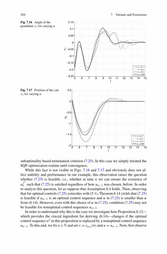
204 7 Variants and Extensions
Fig. 7.16 Angle of thependulum x1 for varying α
Fig. 7.17 Position of the cartx3 for varying α
suboptimality based termination criterion (7.25). In this case we simply iterated theSQP optimization routine until convergence.
While this fact is not visible in Figs. 7.16 and 7.17 and obviously does not af-fect stability and performance in our example, this observation raises the questionwhether (7.25) is feasible, i.e., whether at time n we can ensure the existence ofu
j∗n such that (7.25) is satisfied regardless of how un−1 was chosen, before. In order
to analyze this question, let us suppose that Assumption 6.4 holds. Then, observingthat for optimal controls (7.25) coincides with (5.1), Theorem 6.14 yields that (7.25)is feasible if un−1 is an optimal control sequence and α in (7.25) is smaller than α
from (6.14). However, even with this choice of α in (7.25), condition (7.25) may notbe feasible for nonoptimal control sequences un−1.
In order to understand why this is the case we investigate how Proposition 6.12—which provides the crucial ingredient for deriving (6.14)—changes if the optimalcontrol sequence u� in this proposition is replaced by a nonoptimal control sequenceun−1. To this end, we fix n ∈ N and set x = xμN
(n) and u = un−1. Now, first observe

7.9 Nonoptimal NMPC 205
that the inequalities in (6.12) remain valid regardless of the optimality of u�. Allinequalities in (6.11), however, require optimality of the control sequence u� gener-ating the λn. In order to maintain at least some of these inequalities we can pick anoptimal control sequence u� for initial value xu(1, x) and horizon length N − 1 anddefine a control sequence u via u(0) = u(0), u(n) = u�(n − 1), n = 1, . . . ,N − 1.Then, abbreviating
λn = �(xu(n, x), u(n)
), n = 0, . . . ,N − 1 and
ν = VN
(xu(1, x)
) = VN
(xu(1, x)
),
(7.26)
we arrive at the following version of Proposition 6.12.
Proposition 7.32 Let Assumption 6.4 hold. Then the inequalities
N−1∑
n=k
λn ≤ BN−k(λk) and ν ≤j−1∑
n=0
λn+1 + BN−j (λj+1) (7.27)
hold for k = 1, . . . ,N − 2 and j = 0, . . . ,N − 2.
Proof Analogous to the proof of Proposition 6.12. �
The subtle but crucial difference of (7.27) to (6.11), (6.12) is that the left in-equality in (7.27) is not valid for k = 0. As a consequence, λ0 does not appearin any of the inequalities, thus for any λ1, . . . , λn and ν satisfying (7.27) and anyδ > 0 the values δλ1, . . . , δλn and δν satisfy (7.27), too. Hence, unless (7.27) im-plies ν ≤ ∑N−1
n=0 λn—which is a very particular case—replacing (6.11), (6.12) in(6.14) by (7.27) will lead to the optimal value α = −∞. Consequently, feasibilityof (7.25) cannot be concluded for any positive α.
The following example shows that this undesirable result is not simply due to aninsufficient estimate for α but that infeasibility of (7.25) can indeed happen.
Example 7.33 Consider the 1d system
x+ = x/2 + u (7.28)
with �(x,u) = |x|, input constraint u ≥ 0 and optimization horizon N = 3. A simplecomputation using ux ≡ 0 shows that for this system Assumption 6.4 is satisfiedwith β(r, k) = Cσkr with C = 1 and σ = 1/2. Hence, Corollary 6.19 applies andwe can use (6.19) in order to compute that for N = 3 Inequality (5.1) holds forα = 7/8. If un−1 in the termination criterion (7.25) is chosen as the optimal controlu�, then (7.25) implies that (5.1) is feasible for this α.
For x(n − 1) = 0, it is obvious that the control u� ≡ 0 is optimal. Using thenonoptimal control given by un−1(0) = ε > 0 and un−1(1) = un−1(2) = 0 yieldsthe trajectory xun−1(0) = x(n − 1) = 0, xun−1(k) = ε2−k+1, k = 1,2, which impliesx(n) = ε and
J3(x(n − 1), un−1
) =1∑
k=0
ε2−k = 3ε/2.

206 7 Variants and Extensions
On the other hand, for the initial value x(n) = ε it is easily seen that for each controlun the inequality
J3(x(n),un
) ≥2∑
k=0
ε2−k = 7ε/4 > 3ε/2 = JN
(x(n − 1), un−1
)
holds. Hence, for this choice of un−1 the Inequality (7.25) is not feasible for anyα > 0.
Clearly, in order to rigorously ensure attraction and guaranteed performance oneshould derive conditions which exclude these situations and we briefly discuss twopossible approaches for this purpose.
One way to guarantee feasibility of (7.25) is to add the missing inequality in(7.27) (i.e., the left inequality for k = 0) as an additional constraint in the optimiza-tion. This guarantees feasibility of (7.25) for any α smaller than the value from(6.19). One drawback of this approach is that—similar to the terminal constraintcase—an additional constraint in the optimization is needed which needs to be en-sured for all j ≥ 1 or at least for j∗. This makes the optimization more demanding,since in contrast to Remark 7.27(ii) here we do not have a canonical candidate foran admissible solution which can be used for initializing the iterative optimization.Another drawback is that the value BN(λ0) depends on the in general unknownfunction β from Assumption 6.4 and thus needs to be determined either by an apriori analysis or by a try-and-error procedure.
Another way to guarantee feasibility is to choose � in such a way that there existsγ > 0 for which
γ �(x,u) ≥ �∗(f (x,u))
(7.29)
holds for all x ∈ X and all u ∈ U . Then from (7.29) and the controllability Assump-tion 6.4 for x = f (x(n − 1), un−1(0)) we get
N−1∑
k=0
λk ≤ λ0 + BN−1(�∗(f
(x(n − 1), un−1(0)
))) ≤ λ0 + BN−1(γ λ0).
Replacing β(r,0) by max{β(r, t), β(r, t)} with β(r,0) = β(γ r,0)+ r and β(r, k) =β(γ r, k) for k ≥ 1, this right hand side is ≤ BN(λ0) which again yields the leftinequality in (7.27) for k = 0 and thus feasibility of (7.25). Note that (7.29) holdsfor our example (7.28) if we change �(x,u) = |x| to �(x,u) = |x| + |u|/γ . For this� and the points and control sequences considered in the example, we obtain
J3(x(n − 1), un−1
) = 3ε/2 + ε = 5ε/2
from which one computes that (7.25) is now feasible.The advantage of this method is that no additional constraints have to be imposed
in the optimization. Its disadvantages are that constructing � satisfying (7.29) maybe complicated for more involved dynamics and that the overshoot encoded in β willin general increase for the re-designed �. As outlined in Sect. 6.6, this may lower the

7.10 Beyond Stabilization and Tracking 207
NMPC closed-loop performance and cause the need for larger optimization horizonsN in order to obtain stability.
An in depth study of these approaches and in particular their algorithmic imple-mentation and numerical evaluation will be the topic of further research.
7.10 Beyond Stabilization and Tracking
All NMPC variants discussed so far have in common that the cost function � penal-izes the distance to some desired reference, either to an equilibrium x∗ or to a timevarying reference xref. These variants may hence be called stabilizing NMPC. Thereis, however, a large variety of optimal control problems where this is not the case.For instance, in economic applications one typically uses a running cost �e whichreflects an economic cost rather than a distance to some reference, cf., e.g., Seier-stad and Sydsæter [33]. In what follows we will refer to �e as the economic cost. Insuch problems, the desired limit behavior of the optimal trajectories is not given apriori in terms of a reference x∗ or xref but is rather an outcome of the optimizationitself. Even for rather simple nonlinear models, this limit behavior can be surpris-ingly complex, as, e.g., the examples in the book of Grass, Caulkins, Feichtinger,Tragler and Behrens [12]—for optimal control problems mainly motivated by socialsciences—show.
One way to use stabilizing NMPC for such problems is as follows. In a first step,the optimal limit behavior for the economic running cost �e is identified. Assumingthat this problem can be solved analytically or numerically we obtain an optimalreference solution xref which, however, does not need to be asymptotically stable.Hence, a stabilizing controller needs to be designed in order to stabilize the optimalreference. To this end, in a second step a cost function �—which we will refer toas stabilizing cost—penalizing the distance to xref is designed which is suitable forrunning a stabilizing NMPC scheme in order to obtain a stable closed loop.
Proceeding this way guarantees asymptotic stability of the optimal equilibrium(e.g., under the various conditions on f , � and the particular NMPC scheme dis-cussed in this book) but the resulting closed-loop trajectories based on the optimiza-tion of the stabilizing cost � may be very different from the optimal trajectories usingthe economic cost �e. In particular, they may be far from optimal when performanceis measured via the economic cost function �e.
Due to the fact that for running the NMPC Algorithms 3.1 and its variants no par-ticular conditions on � are needed, it is a natural idea to try to run these algorithmsusing the economic cost �e in (OCPN) and its variants instead of taking the detourvia the stabilizing cost function �. Formally, most usual NMPC algorithms (in par-ticular those discussed in this book) are perfectly suited for doing so, however, thetheoretical results ensuring stability and performance are in general not applicable,because the economic cost �e will not satisfy the conditions needed for these results.Hence, new conditions for ensuring stability and performance are needed.
Here we summarize some recent results in this direction. In [3] (see also the ref-erences in this paper for earlier research on this subject), Angeli, Amrit and Rawl-ings observe that if one adds the optimal limit behavior as a terminal constraint

208 7 Variants and Extensions
to the NMPC scheme, then performance estimates for the NMPC closed loop canbe given. More precisely, assume that the optimal control problem exhibits an op-timal equilibrium x∗ with related control value u∗, i.e., f (x∗, u∗) = x∗ holds and�e(x∗, u∗) is minimal among all possible equilibria. Then, using the NMPC schemefrom Sect. 5.2 with � = �e and X0 = {x∗}, for each x ∈ XN one obtains the perfor-mance estimate
J∞(x,μN) ≤ �e(x∗, u∗), (7.30)
where J∞ denotes the averaged infinite horizon cost functional
J∞(x0,μN) := limK→∞
1
K
K∑
k=0
�e
(xμN
(k, x0),μ(xμN
(k)))
. (7.31)
Observe that J∞(x0,μN) is not simply J∞(x0,μN) from (4.10) with � replaced by�e . The important difference between J∞ and J∞ is that J∞ contains the additionalaveraging term 1/K . This term is necessary since in general for economic runningcosts �e we cannot expect the infinite sum in (4.10) to converge. This approachcan be extended to periodic optimal trajectories xref instead of equilibria by usingsuitable periodic terminal constraint sets; for details see [3].
It is interesting to note that—at least in the case of an optimal equilibrium x∗with control value u∗—the estimate (7.30) may also hold for controllers μN fromstabilizing NMPC schemes. To this end, we use a stabilizing running cost � satisfy-ing
�(x,u) ≥ α1(|x|x∗ + |u|u∗
)(7.32)
for some α1 ∈ K∞ and assume that J∞(x0,μN) is finite and that the economic cost�e is continuous. Then, since J∞(x0,μN) is finite, �e(xμN
(n),μN(xμN(n))) con-
verges to 0 as n → ∞ and hence the lower bound (7.32) implies xμN(n) → x∗ and
μN(xμN(n)) → u∗ as n → ∞. This, in turn, implies �e(xμN
(n),μN(xμN(n))) →
�e(x∗, u∗) as n → ∞ from which (7.30) follows. Hence, although it seems reason-able to expect that for NMPC with economic running cost �e one obtains a betterperformance of the closed-loop trajectories in terms of the economic objective �e ,this is not reflected in the asymptotic estimate (7.30).
In the usual NMPC setting, a finite value of J∞(x0,μN) from (4.10) togetherwith positive definiteness of � allows one to conclude that the closed-loop trajectorymust converge to x∗, because otherwise J∞(x0,μN) would be unbounded. This isnot the case for the averaged functional J∞(x0,μ) from (7.31) and, indeed, oneneeds additional conditions in order to ensure that the closed-loop solution satisfy-ing (7.30) does converge to x∗. Such a condition has been presented in Diehl, Amritand Rawlings [7] for the case of an optimal steady state and finite-dimensional statespace X = R
d . The condition, called strong duality, demands the existence of avalue λ∗ ∈ R
d such that x∗ and u∗ minimize the expression
�e(x,u) + [x − f (x,u)
]Tλ∗

References 209
over all admissible states x ∈ X and control values u ∈ U(x). Furthermore, the exis-tence of α1 ∈ K∞ with
�e(x,u) + [x − f (x,u)
]Tλ∗ − �e(x∗, u∗) ≥ α1
(|x|x∗)
is required. Under these conditions, a Lyapunov function can be constructed byadding suitable correction terms to the finite horizon optimal value function VN (cor-responding to the economic running cost �e). In [2], Angeli and Rawlings furtherobserved that strong duality can be interpreted as a dissipativity condition, whichlinks this condition to more classical concepts used in the stability analysis of con-trol systems.
Summarizing, the results sketched in this section show that NMPC can be usedfor obtaining optimal feedback controllers also for optimal control problems differ-ent from the classical NMPC objectives stabilization and tracking. We conjecturethat NMPC will prove valuable also for other types of optimization criteria, how-ever, we are also convinced that there are problems which are not solvable using thereceding horizon NMPC paradigm. An in depth analysis of the structural propertiesan optimal control problem needs to exhibit in order to be tractable with NMPCtechniques would certainly be an interesting research project.
References
1. Alamir, M.: Stabilization of Nonlinear Systems Using Receding-horizon Control Schemes.Lecture Notes in Control and Information Sciences, vol. 339. Springer, London (2006)
2. Angeli, D., Rawlings, J.B.: Receding horizon cost optimization and control for nonlinearplants. In: Proceedings of the 8th IFAC Symposium on Nonlinear Control Systems – NOL-COS 2010, Bologna, Italy, pp. 1217–1223 (2010)
3. Angeli, D., Amrit, R., Rawlings, J.B.: Receding horizon cost optimization for overly con-strained nonlinear plants. In: Proceedings of the 48th IEEE Conference on Decision and Con-trol – CDC 2009, Shanghai, China, pp. 7972–7977 (2009)
4. Chen, W., Ballance, D.J., O’Reilly, J.: Model predictive control of nonlinear systems: Com-putational delay and stability. IEE Proc., Control Theory Appl. 147(4), 387–394 (2000)
5. De Nicolao, G., Magni, L., Scattolini, R.: Stability and robustness of nonlinear receding hori-zon control. In: Nonlinear Predictive Control, pp. 3–23. Birkhäuser, Basel (2000)
6. Di Palma, F., Magni, L.: On optimality of nonlinear model predictive control. Systems ControlLett. 56(1), 58–61 (2007)
7. Diehl, M., Amrit, R., Rawlings, J.B.: A Lyapunov function for economic optimizingmodel predictive control. IEEE Trans. Autom. Control (2010, in press). doi:10.1109/TAC.2010.2101291
8. Diehl, M., Findeisen, R., Allgöwer, F., Bock, H.G., Schlöder, J.P.: Nominal stability of thereal-time iteration scheme for nonlinear model predictive control. IEE Proc., Control TheoryAppl. 152, 296–308 (2005)
9. Findeisen, R.: Nonlinear model predictive control: A sampled-data feedback perspective. PhDthesis, University of Stuttgart, VDI-Verlag, Düsseldorf (2004)
10. Findeisen, R., Allgöwer, F.: Computational delay in nonlinear model predictive control. In:Proceedings of the International Symposium on Advanced Control of Chemical Processes,Hong Kong, China, 2003. Paper No. 561
11. Graichen, K., Kugi, A.: Stability and incremental improvement of suboptimal MPC withoutterminal constraints. IEEE Trans. Automat. Control 55, 2576–2580 (2010)

210 7 Variants and Extensions
12. Grass, D., Caulkins, J.P., Feichtinger, G., Tragler, G., Behrens, D.A.: Optimal Control of Non-linear Processes. With Applications in Drugs, Corruption, and Terror. Springer, Berlin (2008)
13. Grimm, G., Messina, M.J., Tuna, S.E., Teel, A.R.: Model predictive control: for want of alocal control Lyapunov function, all is not lost. IEEE Trans. Automat. Control 50(5), 546–558(2005)
14. Grüne, L.: Worst case vs. average performance estimates for unconstrained NMPC schemes.PAMM 10, 607–608 (2010)
15. Grüne, L., Pannek, J.: Practical NMPC suboptimality estimates along trajectories. SystemsControl Lett. 58(3), 161–168 (2009)
16. Grüne, L., Pannek, J.: Analysis of unconstrained NMPC schemes with incomplete optimiza-tion. In: Proceedings of the 8th IFAC Symposium on Nonlinear Control Systems – NOLCOS2010, Bologna, Italy, pp. 238–243 (2010)
17. Grüne, L., Rantzer, A.: On the infinite horizon performance of receding horizon controllers.IEEE Trans. Automat. Control 53, 2100–2111 (2008)
18. Grüne, L., Pannek, J., Worthmann, K.: A networked unconstrained nonlinear MPC scheme. In:Proceedings of the European Control Conference – ECC 2009, Budapest, Hungary, pp. 91–96(2009)
19. Grüne, L., Pannek, J., Worthmann, K.: A prediction based control scheme for networked sys-tems with delays and packet dropouts. In: Proceedings of the 48th IEEE Conference on Deci-sion and Control – CDC 2009, Shanghai, China, pp. 537–542 (2009)
20. Grüne, L., Pannek, J., Seehafer, M., Worthmann, K.: Analysis of unconstrained nonlinearMPC schemes with varying control horizon. SIAM J. Control Optim. 48, 4938–4962 (2010)
21. Grüne, L., von Lossow, M., Pannek, J., Worthmann, K.: MPC: implications of a growth con-dition on exponentially controllable systems. In: Proceedings of the 8th IFAC Symposium onNonlinear Control Systems – NOLCOS 2010, Bologna, Italy, pp. 385–390 (2010)
22. Jadbabaie, A., Hauser, J.: On the stability of receding horizon control with a general terminalcost. IEEE Trans. Automat. Control 50(5), 674–678 (2005)
23. Khalil, H.K.: Nonlinear Systems, 3rd edn. Prentice Hall, Upper Saddle River (2002)24. Limón, D., Alamo, T., Salas, F., Camacho, E.F.: On the stability of constrained MPC without
terminal constraint. IEEE Trans. Automat. Control 51(5), 832–836 (2006)25. Michalska, H., Mayne, D.Q.: Robust receding horizon control of constrained nonlinear sys-
tems. IEEE Trans. Automat. Control 38(11), 1623–1633 (1993)26. Nešic, D., Teel, A.R.: A framework for stabilization of nonlinear sampled-data systems based
on their approximate discrete-time models. IEEE Trans. Automat. Control 49(7), 1103–1122(2004)
27. Nešic, D., Grüne, L.: A receding horizon control approach to sampled-data implementation ofcontinuous-time controllers. Systems Control Lett. 55, 660–672 (2006)
28. de Oliveira Kothare, S.L., Morari, M.: Contractive model predictive control for constrainednonlinear systems. IEEE Trans. Automat. Control 45(6), 1053–1071 (2000)
29. Pannek, J.: Receding horizon control: A suboptimality-based approach. PhD thesis, Universityof Bayreuth, Germany (2009)
30. Parisini, T., Zoppoli, R.: A receding-horizon regulator for nonlinear systems and a neuralapproximation. Automatica 31(10), 1443–1451 (1995)
31. Rawlings, J.B., Mayne, D.Q.: Model Predictive Control: Theory and Design. Nob Hill Pub-lishing, Madison (2009)
32. Scokaert, P.O.M., Mayne, D.Q., Rawlings, J.B.: Suboptimal model predictive control (feasi-bility implies stability). IEEE Trans. Automat. Control 44(3), 648–654 (1999)
33. Seierstad, A., Sydsæter, K.: Optimal Control Theory with Economic Applications. North-Holland, Amsterdam (1987)
34. Varutti, P., Findeisen, R.: Compensating network delays and information loss by predictivecontrol methods. In: Proceedings of the European Control Conference – ECC 2009, Budapest,Hungary, pp. 1722–1727 (2009)
35. Zavala, V.M., Biegler, L.T.: The advanced-step NMPC controller: optimality, stability androbustness. Automatica 45(1), 86–93 (2009)

Chapter 8Feasibility and Robustness
In this chapter we consider two different but related issues. In the first part we dis-cuss the feasibility problem, i.e., that the nominal NMPC closed loop solutions re-main inside a set on which the finite horizon optimal control problems defining theNMPC feedback law are feasible. We formally define the property of recursive fea-sibility and explain why the assumptions of the previous chapters, i.e., viability ofthe state constraint set or of the terminal constraint set ensure this property. Thenwe present two ways to relax the viability assumption on the state constraint setin the case that no terminal constraints are used. After a comparative discussionon NMPC schemes with and without stabilizing terminal constraints, we start withthe second part of the chapter in which robustness of the closed loop under addi-tive perturbations and measurement errors is investigated. Here robustness concernsboth feasibility and admissibility as well as stability of the closed loop. We providedifferent assumptions and resulting NMPC schemes for which we can rigorouslyprove such robustness results and also discuss examples which show that in generalrobustness may fail to hold.
8.1 The Feasibility Problem
We start by introducing the feasibility problem for the NMPC Algorithm 3.1, i.e.,for the NMPC formulation without terminal constraints.
Recall from Definition 3.2 that for each x ∈ X the set of admissible control se-quences U
N(x0) is nonempty if and only if there exists a control sequence u ∈ UN
for which the two conditions
u(k) ∈ U(xu(k, x0)
)and xu(k + 1, x0) ∈ X
are satisfied for all k = 0, . . . ,N − 1. Moreover, recall from the discussion afterAssumption 3.3 that the optimization problem (OCPN) in the NMPC Algorithm 3.1is called feasible for the initial value x0 if U
N(x0) �= ∅ holds. Since only feasibleoptimal control problems allow for an admissible solution, the points x0 ∈ X satis-fying U
N(x0) �= ∅ are exactly the points for which the NMPC-feedback law μN is
L. Grüne, J. Pannek, Nonlinear Model Predictive Control,Communications and Control Engineering,DOI 10.1007/978-0-85729-501-9_8, © Springer-Verlag London Limited 2011
211

212 8 Feasibility and Robustness
Fig. 8.1 Infeasible trajectoryfor Example 8.1 with initialvalue x0 = (−1,1)� andoptimization horizon N = 2
well defined. The feasibility problem in NMPC now lies in the fact that even thoughthe constraints xu(n, x0) ∈ X imply xu�(1, x0) = xμN
(1, x0) = f (x0,μN(x0)) ∈ X,it may happen that
UN
(f
(x0,μN(x0)
)) = ∅,
i.e., that the optimization problem (OCPN) for initial value f (x0,μN(x0)) to besolved at next time instant is infeasible. This means that μN and thus also the closed-loop system (2.5) is not defined for x = f (x0,μN(x0)) and the NMPC closed loopruns into a “dead end”.
Example 8.1 We illustrate this fact by Example 3.4, i.e.,
x+ = f (x,u) =(
x1 + x2 + u/2x2 + u
).
We use the state constraints X = [−1,1]2 and the control constraints U(x) = U =[−1/4,1/4]. With the same computation as in Example 3.4 one sees that X is notviable, since, for instance, for the point x = (1,1)� ∈ X we obtain f (x,u) /∈ X forall u ∈ U.
As we have seen in Example 7.2, the system can be stabilized respecting the stateand control constraints starting from the initial value x = (−1,1)�. Running theNMPC Algorithm 3.1 with N = 2 and �(x,u) = ‖x‖2 + 5u2 with this initial value,however, results in the trajectory shown in Fig. 8.1. Here we have not stopped thesimulation upon infeasibility but rather continued the computation with the infeasi-ble solution returned by the optimization algorithm.
Although asymptotically stable, at time n = 3 and 4 this trajectory violates thestate constraints, which are indicated by the black box. Moreover, while the opti-mization algorithm reported infeasibility for n = 1,2,3,4, it terminated success-fully at time n = 0, i.e., the infeasibility at later time instants was not detected uponinitialization and is not due to a failure of the optimization algorithm at time n = 0.

8.1 The Feasibility Problem 213
In order to formally analyze this problem we introduce the following notions.
Definition 8.2 Let a constraint set X and an optimization horizon N ∈ N∞ for theNMPC Algorithm 3.1 be given.
(i) A point x ∈ X is called feasible for X and N if UN(x) �= ∅.
(ii) The feasible set for X and N is defined as
FN := {x ∈ X | x is feasible for X and N}.The set F∞ is also called viability kernel.
(iii) A set A ⊆ X is called recursively feasible for optimization horizon N ∈ N ifA ⊆ FN and it is forward invariant for the NMPC-feedback law μN , i.e., iff (x,μN(x)) ∈ A holds for all x ∈ A.
The recursive feasibility property from Definition 8.2(iii) guarantees that for anyinitial value x ∈ A the NMPC closed loop will generate a solution which is admis-sible for all future times. Formally, this is stated in the following lemma.
Lemma 8.3 Let A ⊆ X be recursively feasible for the NMPC Algorithm 3.1 with op-timization horizon N ∈ N. Then for each x ∈ A the closed-loop solution xμN
(n, x)
generated by (2.5) is well defined for all n ∈ N0 and satisfies xμN(n, x) ∈ A and
thus also xμN(n, x) ∈ X for all n ∈ N0.
Proof The result follows by a straightforward induction using (2.5) and the relationf (x,μN(x)) ∈ A for all x ∈ A. �
Thus, in addition to stability, for proper operation of the NMPC scheme we alsoneed to ensure that the desired operating range of our controller lies in a recur-sively feasible set. Note that xμN
(n, x) ∈ X for all n ∈ N immediately implies theinclusion A ⊆ F∞. For this reason, the viability kernel F∞ is the maximal possiblerecursively feasible subset of X. In particular, it is the maximal set on which an ad-missible feedback can be defined, independent of how this feedback is constructed.
The reason why we did not address the feasibility problem in the previous chap-ters lies in the fact that the assumptions imposed so far always implied feasibility. Infact, in Chap. 6 we always assumed that the constraint set X is viable in the sense ofAssumption 3.3. Under this assumption Theorem 3.5 ensures that A = X is recur-sively feasible, as already remarked after this theorem. However, arbitrary constraintsets are in general not viable. Moreover, while in simple examples the constructionof a viable subset of X may be possible, cf. Example 3.4, for complicated dynamicsthis can be a difficult if not impossible task.
The terminal constrained scheme discussed in Chap. 5 provides a remedy tothis problem. For this scheme, recursive feasibility of XN is always ensured byLemma 5.3. However, the price that we pay for this nice property is that the op-erating range is a priori restricted to XN , which may be considerably smaller thanthe operating range of the unconstrained scheme, cf. Example 6.2. Furthermore, we

214 8 Feasibility and Robustness
either need to impose equilibrium constraints X0 = {x∗}—which may be too re-strictive for some systems and may cause problems in the numerical optimizationroutine—or we need to find a viable terminal constraint set X0 along with a terminalcost F defined on X0 which satisfies Assumption 5.9. While the design of F canbe avoided by using the mixed scheme from the first part of Sect. 7.1, in any casewe need to find a viable terminal constraint set X0. Note that finding this “small”set is in general easier than finding a “big” viable state constraint set X. However,both in terms of the operating range of the scheme and in terms of implementa-tional simplicity, it would be desirable if we could use the unconstrained schemewithout having to worry about the feasibility problem and without having to con-struct a viable terminal constraint set X0. In the following sections we will showtwo approaches in this direction.
8.2 Feasibility of Unconstrained NMPC Using Exit Sets
In this and in the subsequent section we present two results which ensure feasibilityfor the unconstrained NMPC Algorithm 3.1 under two different assumptions. Whilethe first result uses properties of the interplay between the dynamics f and theconstraint set X and is independent of any stability properties, the second approachuses asymptotic stability of the closed loop in order to ensure feasibility of subsetsof the state space.
In order to introduce our first approach we need the following objects.
Definition 8.4 Consider a control system (2.1) with state constraint set X ⊂ X andcontrol constraint set U(x) ⊆ U , x ∈ X. We recursively define the exit sets Ek ⊆ X,k ∈ N0 as
E0 := X \ X,
Ek :={
x ∈ X
∣∣∣ f (x,u) ∈k−1⋃
i=0
Ei for all u ∈ U(x)
}
, k = 1,2, . . . .
Remark 8.5
(i) This definition immediately implies Ek′ ⊆ Ek for all k ≥ k′ ≥ 1.(ii) If X is viable then the definition of E0 implies E1 = ∅ and thus by induction
Ek = ∅ for all k ≥ 1.
In words, for k ≥ 1 the exit set Ek consists of all points x0 ∈ X for which it isunavoidable that the trajectory xu(k, x0) leaves X after at most k steps regardless ofhow u ∈ U
k(x0) is chosen. This is made precise in the following lemma.

8.2 Feasibility of Unconstrained NMPC Using Exit Sets 215
Lemma 8.6 A point x ∈ X satisfies x ∈ Ek if and only if the following propertyholds:
for each u ∈ Uk there exists ku ∈ {0, . . . , k} such that either
u(n) /∈ U(xu(n, x)
)for some n ∈ {0, . . . , ku − 1} or xu(ku, x) /∈ X.
(8.1)
Proof We show the property by induction over k. For k = 0 the assertion followsimmediately from E0 = X \ X and xu(0, x) = x. For the induction step k → k + 1assume that the assertion holds for k. We then need to show that x ∈ Ek+1 holds ifand only if (8.1) holds for k + 1.
We first show that (8.1) holds for x ∈ Ek+1. Let x ∈ Ek+1 and pick u ∈ Uk+1.If u(0) /∈ U(x), then (8.1) holds with ku = 1. Hence, assume u(0) ∈ U(x). Thenwe get x ′ = xu(1, x) ∈ Ei for some i ∈ {0, . . . , k}. Now, by induction assumptionfor the shifted control u′ = u(· + 1) ∈ Uk there exists ku′ ∈ {0, . . . , k} such thateither u′(n) /∈ U(xu′(n, x′)) for some n ∈ {0, . . . , ku′ − 1} or xu′(ku′, x′) /∈ X. Sinceu′(n) = u(n + 1) and xu′(ku′, x ′) = xu(ku, x) for ku = ku′ + 1 ≤ k + 1, this showsthat (8.1) holds for ku = ku′ + 1.
Conversely, given x ∈ X for which (8.1) holds for k + 1, we need to show x ∈Ek+1. Let ux ∈ U(x) be given and denote x ′ = f (x,ux). We have to show thatx′ ∈ Ei for some i ≤ k. If x′ /∈ X then x′ ∈ E0 and we are done. Otherwise, we pickan arbitrary control sequence u′ ∈ Uk for x ′ and define a control sequence u ∈ Uk+1
by setting u(0) = ux and u(j) = u′(j − 1) for j ∈ {1, . . . , k}. Then by (8.1) thereexists ku ≤ k + 1 such that either u(n) /∈ U(xu(n, x)) for some n ∈ {0, . . . , ku − 1}or xu(ku, x) /∈ X and since xu(1, x) = x ′ ∈ X we know that ku ≥ 1. By constructionof u this implies that (8.1) holds for x′ and u′ with ku′ = ku − 1 ≤ k. Hence, by theinduction assumption x′ ∈ Ek and consequently by definition of the Ek we obtainx ∈ Ek+1. �
Our next lemma shows the relation between the exit sets Ek and the feasible setsFN from Definition 8.2(ii).
Lemma 8.7 Consider a control system (2.1) with state constraint set X ⊂ X andcontrol constraint set U(x), x ∈ X. Then the identity
FN = X \ EN = X
∖(N⋃
k=1
Ek
)
(8.2)
holds for all N ∈ N.
Proof The second equality follows immediately from Remark 8.5(i). It remains toshow FN = X \ EN , which we will do by proving “⊆” and “⊇”.
“⊆”: Consider x ∈ FN . Then UN(x) is nonempty, hence we can pick u ∈ U
N(x).By definition of U
N(x) this implies u(k) ∈ U(xu(k, x)) for all k = 0, . . . ,N − 1 andxu(k, x) ∈ X for k = 0, . . . ,N . Thus, (8.1) does not hold and Lemma 8.6 impliesx /∈ EN and thus x ∈ X \ EN .

216 8 Feasibility and Robustness
“⊇”: Let x ∈ X \EN , i.e., x ∈ X and x /∈ EN . Then Lemma 8.6 implies that (8.1)does not hold, i.e., there exists u ∈ UN with u(n) ∈ U(xu(n, x)) for n = 0, . . . ,N −1and xu(n, x) ∈ X for n = 0, . . . ,N . This means that u ∈ U
N(x), hence UN(x) �= ∅
and consequently x ∈ FN . �
Remark 8.8 If f is continuous then one can also show F∞ = X \ (⋃∞
k=1 Ek).
Now we introduce the assumption we will use in order to guarantee feasibility.
Assumption 8.9 There exists N0 ∈ N0 such that Ek ⊆ EN0 for all k ≥ N0.
By Remark 8.5(ii) this assumption is satisfied for N0 = 0 if X is viable. Thus,Assumption 8.9 can be seen as a relaxation of Assumption 3.3. In Example 8.12,below, we will see that this condition is satisfied for the system from Example 8.1.However, before we look at this example we show that under this assumption thefeasible set FN0 becomes recursively feasible for optimization horizon N ≥ N0 + 1.To this end we need another preparatory lemma.
Lemma 8.10 Under Assumption 8.9 the identity
F∞ = FN
holds for all N ≥ N0.
Proof First observe that Assumption 8.9 together with Lemma 8.7 immediately im-plies FN = FN0 for all N ≥ N0. Thus, it is sufficient to show the assertion forN = N0.
Since the inclusion F∞ ⊆ FN follows directly from the definition, it remainsto show the converse inclusion. Thus, we need to prove that U
∞(x) �= ∅ for allx ∈ FN0 . We do this by constructing u ∈ U
∞(x). To this end, since FN0 = FN0+1,we can pick u0 ∈ U
N0+1(x) and set u(0) := u0(0). Then the definition of UN(x)
implies u0(· + 1) ∈ UN0(x1) for x1 = xu0(1, x) = xu(1, x). Thus x1 ∈ FN0 = FN0+1
and we can find u1 ∈ UN0+1(x1). Setting u(1) := u1(0) with the same arguments we
obtain u1(·+1) ∈ UN0(x2) for x2 = xu1(1, x1) = xu(2, x). Proceeding iteratively we
obtain a control sequence u ∈ U∞ which satisfies xk = xu(k, x) = xuk−1(1, xk−1) ∈
FN0+1 ⊆ X and u(k) = uk(0) ∈ U(xk) = U(xu(k, x)) for all k ∈ N0. Thus u ∈U
∞(x). �
Using Lemma 8.10 we can now prove our first recursive feasibility result.
Theorem 8.11 Consider the NMPC Algorithm 3.1 and let Assumption 8.9 hold.Then the feasible set FN0 = F∞ is recursively feasible for all optimization horizonsN ≥ N0 + 1.
Proof Consider x ∈ FN0 . Since by Lemma 8.10 the identity FN0 = FN holds, inparticular we obtain FN0 ⊆ FN . Hence, problem (OCPN) in Algorithm (3.1) is fea-sible. Let u� be the corresponding optimal control which implies μN(x) = u�(0).

8.3 Feasibility of Unconstrained NMPC Using Stability 217
Since u� ∈ UN(x) the definition of U
N(x) implies u�(· + 1) ∈ UN−1(xu�(1, x)) =
UN−1(f (x,μN(x))). Thus, U
N−1(f (x,μN(x))) �= ∅ and hence f (x,μN(x)) ∈FN−1. Since N − 1 ≥ N0, Lemma 8.10 yields FN−1 = FN0 . This showsf (x,μN(x)) ∈ FN0 , i.e., FN0 is recursively feasible. �
Example 8.12 We illustrate Assumption 8.9 and Theorem 8.11 by means of Exam-ple 3.4 and 8.1, i.e.,
x+ = f (x,u) =(
x1 + x2 + u/2x2 + u
).
As in the previous examples we use the state constraints X = [−1,1]2. The controlconstraints are chosen more generally as U(x) = U = [−u, u] with u > 0.
A straightforward but tedious computation shows that the exit sets Ek are givenby
Ek =k⋃
j=1
{x ∈ [−1,1]2
∣∣ x1 > −jx2 + 1 + j2u/2 or x1 < jx2 − 1 − j2u/2
}.
In Example 3.4 we chose u = 1. With this parameter one sees that Ek = E1 forall k ≥ 1 because the inequalities for j ≥ 2 are never satisfied for x ∈ [−1,1]2.Hence, Assumption 8.9 is satisfied with N0 = 1 and Theorem 8.11 yields that theset F1 = F∞ = X \ E1 from Lemma 8.7 is recursively feasible for all N ≥ 2. Thisset is exactly the set defined in (3.6).
In Example 8.1 we have u = 1/4. In this case one sees that E4 �= E3 because(−0.99,1)� ∈ E4 but (−0.99,1)� /∈ E3. On the other hand, Ek = E4 for all k ≥ 4because for x2 ∈ [−1,1] and j ≥ 5 the inequality
−jx2 + 1 + j2u/2 > −4x2 + 1 + 42u/2
holds. Hence, the inequality for j = 4 is always satisfied whenever the inequalityfor some j ≥ 5 is satisfied, thus x ∈ Ej for j ≥ 5 implies x ∈ E4. Consequently,Assumption 8.9 holds with N0 = 4 and according to Theorem 8.11 for Example 8.1the closed-loop solution satisfies the state constraints for N ≥ 5 and all x ∈ X \ E4.In particular, since the point (−1,1)� is not contained in E4, the infeasibility fromFig. 8.1 should disappear. Figure 8.2 shows that this is exactly what happens.1
8.3 Feasibility of Unconstrained NMPC Using Stability
A main advantage of the feasibility analysis in the previous section is that it is com-pletely independent of any stability properties of the closed loop. Thus, feasibilityand stability can be analyzed independently of each other. Unfortunately, Theo-rem 8.11 crucially relies on Assumption 8.9 which may not be satisfied for many
1In fact, the infeasibility already disappears for N = 3 and N = 4 but this is not covered by ourtheorem.

218 8 Feasibility and Robustness
Fig. 8.2 Feasible trajectoryfor Example 8.1 with initialvalue x0 = (−1,1)� andoptimization horizon N = 5
practical problems and, even if it is satisfied, may be difficult to verify for complexdynamics.
Thus, in this section we present an alternative result which shows that feasibilitymay be inherited from the optimality properties of the solution and from the stabilityof the closed loop. In order to derive this result we first need three basic assumptionsand a couple of preparatory lemmas.
Our stability results rely on the controllability Assumption 6.4, which is onlymeaningful if the state constraint set X is viable. If this is not the case, then asymp-totic controllability for arbitrary horizons N only makes sense for initial valuesx ∈ F∞. This is what our first assumption demands.
Assumption 8.13 Consider the optimal control problem (OCPN) with a not nec-essarily viable state constraint set X. We assume that on the viability kernel F∞the system is asymptotically controllable with respect to � with rate β ∈ K L0,i.e., for each x ∈ F∞ and each N ∈ N there exists an admissible control sequenceux ∈ U
N(x) satisfying xux (n, x) ∈ F∞ for all n = 1, . . . ,N and
�(xux (n, x),ux(n)
) ≤ β(�∗(x), n
)
for all n ∈ {0, . . . ,N − 1} and �∗ from (6.2).
Under this assumption the results from the stability analysis in Chap. 6 remainvalid if we replace the state constraints xu(k, x) ∈ X for k = 0, . . . ,N (which in(OCPN) is implicitly expressed by the requirement u ∈ U
N(x)) by the state con-straints
xu(k, x) ∈ F∞ for k = 0, . . . ,N. (8.3)
Indeed, since F∞ is viable the standing assumption from Chap. 6, cf. Remark 6.22,is satisfied for these stricter state constraints, i.e., if we replace X by F∞. Further-more, from the observation in Remark 6.11 it follows that the results from Chap. 6remain valid if we replace the constraint for k = N in (8.3) by a weaker constraint.
8.3 Feasibility of Unconstrained NMPC Using Stability 219
In particular, Theorem 6.14 remains valid for β from Assumption 8.13 and F∞ inplace of X if we weaken (8.3) to
xu(k, x) ∈ F∞ for k = 0, . . . ,N − 1, xu(N,x) ∈ X. (8.4)
In the remainder of this section, the reference (OCPN) will always refer to the prob-lem with the original state constraints xu(k, x) ∈ X, k = 0, . . . ,N , while we will al-ways explicitly refer to (8.4) if we consider (OCPN) with the additional constraints(8.4).
In order to apply our stability results from Chap. 6, we need further assump-tions on � and VN . For this assumption recall once again the definition �∗(x) :=infu∈U �(x,u) from (6.2).
Assumption 8.14 There exist α1, α2, α3, α4 ∈ K∞ and N0 ≥ 2 such that the in-equalities
α1(|x|x∗
) ≤ VN(x) ≤ α2(|x|x∗
)
and
α3(|x|x∗
) ≤ �∗(x) ≤ α4(|x|x∗
)
hold for all N ≥ N0.
Note that the assumptions of Theorem 6.21 imply Assumption 8.14 with α1 = α3and α2(r) = ∑∞
k=0 β(α4(r), k). Here the linearity and summability of β ensure thatα2 is indeed a K∞-function.
Finally, we want to ensure that the feedback stabilization problem under the givenstate constraints X is solvable locally around x∗. A prerequisite for this is that thereexists a neighborhood of x∗ whose intersection with X consists of points which arefeasible for N = ∞. This is our last assumption.
Assumption 8.15 There exists a ball Bδ(x∗) such that Bδ(x∗) ∩ X ⊆ F∞.
Observe that we only require the inclusion Bδ(x∗) ∩ X ⊆ F∞ (as opposed toBδ(x∗) ⊆ F∞), which allows for the situation that x∗ is on the boundary of X.
The following two lemmas show properties of optimal trajectories which arecrucial for our feasibility analysis.
Lemma 8.16 Assume that Assumptions 8.13–8.15 hold. Let ε = α−12 ◦ α3(δ) > 0
with α2, α3 ∈ K∞ from Assumption 8.14 and δ > 0 from Assumption 8.15. Thenfor each N ≥ 2 and each x ∈ Bε(x∗) ∩ X the optimal trajectory for OCPN satisfiesxu�(n, x) ∈ Bδ(x∗) ∩ X for all n ∈ {0, . . . ,N − 1}.
Proof The relation xu�(n, x) ∈ X follows immediately from u� ∈ UN(x). It remains
to show xu�(n, x) ∈ Bδ(x∗). From the inequality for �∗ in Assumption 8.14 we ob-tain
�(y,u) ≥ α3(δ) for all y /∈ Bδ(x∗). (8.5)
220 8 Feasibility and Robustness
On the other hand, the inequality for VN in Assumption 8.14 and the definition of ε
imply
VN(x) < α2(ε) = α2(α−1
2 ◦ α3(δ)) = α3(δ) for all x ∈ Bε(x∗). (8.6)
Now assuming xu�(n, x) /∈ Bδ(x∗) for some x ∈ Bε(x∗) and some n ∈ {0, . . . ,N −1}, and using (8.5) with y = xu�(n, x) implies
VN(x) =N−1∑
k=0
�(xu�(k, x), u�(k)
) ≥ �(xu�(n, x),u�(n)
) ≥ α3(δ),
which contradicts (8.6). �
Lemma 8.17 Assume that Assumptions 8.13–8.15 hold and consider some ε > 0.Let N ≥ 2 and x ∈ FN with VN(x) < Nα3(ε). Then the optimal trajectory xu�(n, x)
for (OCPN) satisfies xu�(n, x) ∈ Bε(x∗) ∩ X for some n ∈ {0, . . . ,N − 1}.
Proof Again, xu�(n, x) ∈ X follows immediately from u� ∈ UN(x) and it remains
to show xu�(n, x) ∈ Bε(x∗). To this end, assume xu�(n, x) /∈ Bε(x∗) for all n ∈{0, . . . ,N − 1}. Then Assumption 8.14 implies
VN(x) =N−1∑
k=0
�(xu�(k, x), u�(k)
) ≥N−1∑
k=0
α3(∣∣xu�(k, x)
∣∣x∗
) ≥ Nα3(ε),
which contradicts VN(x) < Nα3(ε). �
The next lemma shows a property of arbitrary admissible trajectories.
Lemma 8.18 Let N ∈ N, x ∈ FN and u ∈ UN(x) be such that the correspond-
ing trajectory satisfies xu(N − 1, x) ∈ F∞. Then xu(k, x) ∈ F∞ for all k =0, . . . ,N − 1.
Proof Fix an arbitrary k ∈ {0, . . . ,N − 2} and abbreviate xk = xu(k, x). Since y =xu(N − 1, x) ∈ F∞ there exists a control sequence uy ∈ U
∞(y), i.e.,
uy(n) ∈ U(xuy (n, y)
)and xuy (n, y) ∈ X
for all n ∈ N0. Then the concatenated control sequence
u(n) ={
u(n + k), n = 0, . . . ,N − k − 2,
uy(n − N + k + 1), n ≥ N − k − 1
and the initial value xk yield a trajectory satisfying
xu(n, xk) ={
xu(n + k, x), n = 0, . . . ,N − k − 1,
xuy (n − N + k + 1, y), n ≥ N − k − 1.
This trajectory remains in X for all n ≥ 0 and the corresponding control sequence u
is admissible for all times. Thus u ∈ U∞(xk), hence U
∞(xk) �= ∅ and consequentlyxk ∈ F∞. �
Combining the three previous lemmas we arrive at the following proposition.

8.3 Feasibility of Unconstrained NMPC Using Stability 221
Proposition 8.19 Assume that Assumptions 8.13–8.15 hold and let N ≥ 2 and x ∈FN with VN(x) < Nα3 ◦ α−1
2 ◦ α3(δ) with α2, α3 ∈ K∞ from Assumption 8.14 andδ > 0 from Assumption 8.15. Then the optimal trajectory xu�(n, x) for (OCPN) withhorizon N satisfies xu�(n, x) ∈ F∞ for all n ∈ {0, . . . ,N − 1}.
In particular, for these x the optimal values and the optimal trajectories do notchange if we add the constraints (8.4) to the optimal control problem (OCPN).
Proof Applying Lemma 8.17 with ε = α−12 ◦ α3(δ) yields xu�(n, x) ∈ Bε(x∗) for
some n ∈ {0, . . . ,N − 1}. Since by Corollary 3.16 the trajectory xu�(n + ·, x) isoptimal for horizon N −n and initial value xu�(n, x), Lemma 8.16 yields xu�(k, x) ∈
Bδ(x∗)∩X for k = n, . . . ,N −1. In particular, this implies xu�(N −1, x) ∈ Bδ(x∗)∩X ⊆ F∞. Now Lemma 8.18 yields the assertion. �
Now we are ready to formulate our feasibility theorem.
Theorem 8.20 Let Assumptions 8.13–8.15 hold, let N ≥ 2 and assume that α fromTheorem 6.14 with β from Assumption 8.13 satisfies α ∈ (0,1]. Then the set
A = {x ∈ FN
∣∣ VN(x) < Nα3 ◦ α−12 ◦ α3(δ)
}
with α2, α3 ∈ K∞ from Assumption 8.14 and δ > 0 from Assumption 8.15 is recur-sively feasible for the NMPC feedback μN from Algorithm 3.1. Furthermore, theNMPC closed loop (2.5) is asymptotically stable on A.
Proof From the discussion after Assumption 8.13 it follows that Theorem 6.14 isapplicable for Algorithm 3.1 with the additional constraints (8.4) in (OCPN) withβ from Assumption 8.13. Thus, (5.1) holds for μN from Algorithm 3.1 and thecorresponding optimal value function VN for all x ∈ F∞ if we add the constraints(8.4).
By Proposition 8.19, for x ∈ A the optimal trajectories do not change if we addthe constraints (8.4) to the optimal control (OCPN) in Algorithm 3.1. In particu-lar, this implies that the resulting NMPC feedback μN does not change if we addthe state constraints (8.4). Since, furthermore, for x ∈ A the optimal trajectories of(OCPN) lie in F∞, we get x ∈ F∞ and f (x,μN(x)) ∈ F∞, thus VN is defined in x
and f (x,μN(x)). Hence, for each x ∈ A (5.1) also holds for μN from Algorithm 3.1and the corresponding optimal value function VN without the constraints (8.4). Forx ∈ A this implies
VN
(f
(x,μN(x)
)) ≤ VN(x) − α�(x,μN(x)
) ≤ VN(x) < Nα3 ◦ α−12 ◦ α3(δ)
and thus f (x,μN(x)) ∈ A. This shows the recursive feasibility of A. �
Corollary 8.21 Let Assumptions 8.13–8.15 hold, let N0 ≥ 2 and assume that α
from Theorem 6.14 with β from Assumption 8.13 satisfies α ∈ (0,1] for all N ≥N0. Then for each bounded set K ⊆ F∞ there exists NK ≥ N0 such that for eachN ≥ NK there exists a recursively feasible set AN for the NMPC feedback μN
from Algorithm 3.1 with K ⊆ AN . Furthermore, the NMPC closed loop (2.5) is

222 8 Feasibility and Robustness
asymptotically stable on AN . In particular, if X is bounded, then F∞ is recursivelyfeasible for all sufficiently large optimization horizons N .
Proof Using the upper bound α2 on VN from Assumption 8.14 and the inclusionF∞ ⊆ FN it follows that the set A from Theorem 8.20 contains the set Bν(x∗)∩ F∞with
ν = α−12
(Nα3 ◦ α−1
2 ◦ α3(δ)).
Since ν ↗ ∞ for N → ∞, for each bounded set K ⊆ F∞ we can chooseNK ≥ N0 such that K ⊆ Bν(x∗) ∩ F∞ holds for all N ≥ NK . This shows the claimfor AN = A. �
8.4 Comparing Terminal Constrained vs. Unconstrained NMPC
Now that we have developed the main stability and feasibility results we will discussthe main advantages and disadvantages of NMPC schemes with and without termi-nal constraints and/or costs. More precisely we distinguish between the followingschemes.
(a) NMPC with equilibrium (or time varying reference) endpoint constraint fromSect. 5.2
(b) NMPC with Lyapunov function terminal cost from Sect. 5.3(c) NMPC without terminal cost and constraints from Chap. 6
We compare the main features of these NMPC variants in terms of
(i) design, i.e., the choice of the necessary ingredients of the respective algorithms(ii) stability, i.e., the asymptotic stability properties of the closed loop and the as-
sumptions needed in order to guarantee them(iii) performance, i.e., the suboptimality compared with the infinite horizon optimal
value(iv) feasibility, i.e., the guarantee that the optimal control problem in the NMPC
closed loop is solvable for the given constraints(v) numerical effort, i.e., the time needed for the online optimization
(i) Regarding the design, clearly the schemes (a) and (c) are preferable. In bothcases all that needs to be designed is a desired equilibrium (or reference in the timevarying case) and a running cost � which is positive definite with respect to thisreference, which in the simplest case could be of the form (3.3).
In contrast to this, the additional construction of a viable terminal constraint setX0 and a terminal cost F meeting Assumptions 5.1(i) and (ii) necessary for (b)poses a considerable additional difficulty in the design of the scheme, notably (butnot exclusively) for time varying references.
This is probably the main reason for the fact that in our discussion with prac-titioners the formulations (a) and (c) turned out to be the by far preferred NMPCvariants in industrial applications.

8.4 Comparing Terminal Constrained vs. Unconstrained NMPC 223
(ii) The main difference of the stability properties for the different schemes liesin the fact that for (a) and (b) the operating range, i.e., the region on which thestabilizing feedback is defined or, equivalently, the domain of attraction of the ref-erence solution for the closed-loop solution, is a priori confined to the feasible setXN . In contrast to this, the unconstrained scheme (c) can yield larger and even un-bounded stability regions for fixed N , cf. Example 6.2. On the other hand, for smalloptimization horizons N in (a) and (b) only the domain of attraction shrinks whilefor (c) asymptotic stability may be lost completely. Which of the two advantages isdominant can only be assessed on a case by case basis for each particular system tobe controlled, usually performed with the support of numerical simulations and/orexperimental results.
Regarding the conditions for stability, (a) requires the system to be controllableto the desired reference point or trajectory in finite time, while (b) requires the via-bility of the terminal constraint set X0 and the compatibility of F and � in the senseof Assumption 5.1(ii). The unconstrained scheme, in turn, requires the asymptoticcontrollability from Assumption 6.4 or the bound from Assumption 6.30 and a pos-itive value α in Theorem 6.14 or a sufficiently large optimization horizon N , cf.Theorem 6.33. The conditions for the existence of suitable F and � for (b) and � for(c), respectively, can roughly be regarded as comparably strong as they both essen-tially require asymptotic controllability with suitable uniformity. In contrast to this,the finite time controllability condition for (a) is stronger.
Concerning the verification of these conditions, the assumptions for (a) and (b)are in typically considerably easier to check than the asymptotic controllability con-dition for (c). However, a considerable difference between the conditions for (b)and (c) is that F in (b) must be constructed in order to run the scheme while β inAssumption 6.4 is only needed for the analysis of the scheme but not at runtime.
(iii) Regarding performance, the respective Theorems 5.21 and 6.21 show thatfor all schemes (a)–(c) the infinite horizon performance J∞(x,μN) from Defini-tion 4.10 approaches the optimal value V∞(x) if the optimization horizon N tendsto infinity. The conditions for these theorems to hold are essentially equivalent toconditions needed for asymptotic stability. For scheme (b), Theorem 5.22 gives analternative estimate under an assumption on the terminal cost F .
For fixed N , however, not only the operating range (cf. Example 6.2 and thediscussion in (ii), above) but also the performance may differ, at times considerably,even if XN = X holds. We illustrate this effect by two examples.
Example 8.22 We reconsider Examples 5.18 and 6.1, i.e.,
x+ = x + u, �(x,u) = x2 + u2
with X = X = U = U = R. In Example 5.18 we computed that scheme (a) for N = 2yields the controller μ2(x) = 2x/3 satisfying J∞(x,μ2) = 1.625x2.

224 8 Feasibility and Robustness
In Example 6.1 it turned out that for the same example from scheme (c) we obtainthe controller μ2(x) = −x/2. This yields the closed-loop solution xμ2(k, x) = x/2k
and �(x,μ2(x)) = x2 + (x/2)2 = 5x2/4. This implies
J∞(x,μ2) =∞∑
k=0
�(xμ2(k, x),μ2
(xμ2(k, x)
)) =∞∑
k=0
5
4
x2
22k= 5
3x2 ≈ 1.666x2
(note that this value coincides with the upper bound V2(x)/α from Theorem 6.18since in Example 6.1 we computed V2(x) = 3x2/2 and α = 0.9, hence V2(x)/α =(3x2/2)(10/9) = 5x2/3). Hence, for this example scheme (a) yields a better perfor-mance than scheme (c).
Example 8.23 Consider again Example 5.19, i.e.,
x+ = x + u, �(x,u) = x2 + u4
with X = X = U = U = R. In this example we showed that scheme (a) yields
J∞(20,μ2) ≈ 11240.39.
On the other hand, the controller μ given in Example 5.19 is nothing but the con-troller μ2 for scheme (c), which we again computed by MAPLE. This controlleryields
J∞(20,μ2) ≈ 1725.33,
i.e., a considerably better value.
Roughly speaking, the terminal constraints employed in (a) and (b) cause theNMPC-feedback law to steer the system to the equilibrium or reference more rapidlyat the cost of larger control effort, while the unconstrained scheme (c) typically actsmore cautiously. This is why in Example 8.22, in which the control is only moder-ately penalized, scheme (a) performs better while in Example 8.23, in which largecontrol values are penalized much more heavily, scheme (c) yields the better re-sult. In general, it appears that for a stronger penalization of the control effort theunconstrained scheme (c) provides better performance. It should, however, also bementioned that a stronger penalization of u typically yields a larger β in Assump-tion 6.4, which in turn may affect the stability of scheme (c).
(iv) Our discussion on feasibility from the last sections shows that for the ter-minal constrained schemes (a) and (b) the sets XN are “automatically” recursivelyfeasible. This property is inherited from the viability of the terminal constraint setX0. For the unconstrained scheme recursive feasibility can be expected on (a sub-set of) the viability kernel, as Theorems 8.11 and 8.20 as well as Corollary 8.21show. However, in contrast to (a) and (b) here we need additional assumptions anda sufficiently large optimization horizon N if the state constraint set X itself is notviable.
Regarding the detection of infeasibility, the schemes (a) and (b) have the advan-tage that feasibility of the nominal closed loop is guaranteed once the optimizationalgorithm reports that (OCPN,e) has a feasible solution for the initial value x0. In

8.5 Robustness: Basic Definition and Concepts 225
contrast to this, in scheme (c) infeasibility may occur even if (OCPN) has a feasi-ble solution for the initial value, cf. Example 8.1. Thus, in schemes (a) and (b) theinfeasibility is usually detected earlier than in scheme (c).
(v) The numerical effort depends on many different parameters, most notablyon the dimension of the problem, on the optimization horizon, on the structure ofthe dynamics f and the running cost � and on the number and type of constraints.Generally, one has to take into account that in a nonlinear and nonconvex settingit can often not be expected that the optimization algorithm is able to find a globaloptimum. The reason for this will become apparent in the discussion of nonlinearoptimization algorithms in Chap. 10. Hence, in general it is difficult to assess whichof the schemes is preferable from the numerical point of view.
However, regarding the constraints it is clear that the schemes (a) and (b) aremore demanding than (c). In particular, the endpoint constraint of scheme (a) maycause severe problems in the numerical optimization routine for nonlinear and non-convex problems. From this point of view the regional constraint in scheme (b) istypically preferable to (a) and scheme (c) without terminal constraints is certainlythe best of all. However, if the terminal constraint helps to significantly reduce theoptimization horizon N in scheme (a) or (b) compared to scheme (c), e.g. whenno good running cost in the sense of Sect. 6.6 can be found for (c), then this effectmay easily override the advantage of having fewer constraints in scheme (c). Hence,similar to what was said in the discussion in the first paragraph of (ii), again an as-sessment on a case by case basis must be made in order to decide which scheme ismore appropriate for a given system and control task.
Summarizing the discussion in this section, one sees that both terminal con-strained and unconstrained schemes have their specific advantages and disadvan-tages. In practice, it is presumably a good choice to start with an unconstrainedscheme which is easier to design and assess its performance via numerical sim-ulations and practical experiments. If the desired performance—be it in terms ofstability, suboptimality or feasibility—is not achieved for reasonable choices of N
and simple modifications like, e.g., the terminal weights from Sect. 7.2 do not yielda solution, then one of the more sophisticated methods like adding appropriate ter-minal constraints and costs, a redesign of the running cost functions in the spirit ofSect. 6.6 or one of the mixed schemes from Sect. 7.1 should be considered.
8.5 Robustness: Basic Definition and Concepts
Real systems do never exactly coincide with their mathematical models. This meansthat in practice the behavior of the real system will deviate from the mathematicallyidealized model (2.1). In this and in the following sections we will analyze the im-pact of these deviations on the NMPC closed loop and discuss NMPC variants whichprovide robustness against such errors. In order to simplify the setting we will con-sider the case of time invariant reference xref = x∗. All result do, however, carryover to the time varying case provided the necessary assumptions hold uniformlywith respect to time; we will comment on this in remarks after our main results.

226 8 Feasibility and Robustness
Sources for errors are, for instance, modeling errors, uncertain parameters, exter-nal disturbances acting on the system and measurement errors. A further source arenumerical errors, which are almost inevitable in NMPC schemes because we need anumerical integration scheme for the solution of (OCPn
N,e) or its variants. This topicwill be treated in detail in Chap. 9, see in particular Sect. 9.5.
As a consequence, the predicted trajectories xu(k, x) used in (OCPnN,e) and its
variants do not exactly coincide with the future behavior of the real system.Formally, we have already taken this fact into account by referring to the closed-
loop systems (2.5) and (3.5) as nominal closed-loop system. Recall that the nominalNMPC closed loop (3.5) whose behavior we analyzed in the preceding chapters andsections is given by
x+ = f(x,μN(x)
).
Here f exactly coincides with f in (2.1), which is used in (OCPnN,e) or its variants
to compute the NMPC controller μN .In order to analyze the influence of the various error sources, for simplicity of
exposition we assume that our state space X is a normed vector space such that wecan add elements of X and measure the size of elements x ∈ X by their norm ‖x‖.Then we can introduce the perturbed closed-loop model
x+ = f(x,μN(x + e)
) + d. (8.7)
Here d ∈ X is an additive perturbation which covers all kinds of errors causing f todeviate from the evolution of the real system, like modeling and numerical errors,external disturbances, uncertain parameters etc. In addition, we consider the errorterm e ∈ X, which models measurement errors. Note that when both f and μN arecontinuous then one could express the effects of d and e on the system via oneadditive perturbation d . However, while all of our robustness results will rely onthe continuity of f we will not assume continuity of μN because optimal feedbackcontrols and thus NMPC-feedback laws are, in general, discontinuous.
In order to distinguish between the nominal and the perturbed system, we denotethe states of the perturbed system by x and the states of the nominal model by x. Forinitial value x0 ∈ X and sequences of perturbation values d(·), e(·) ∈ XN we obtainsolutions xμN
(k, x0) of (8.7) from the iteration
xμN(0, x0) = x0,
xμN(k + 1, x0) = f
(xμN
(k, x0),μN
(xμN
(k, x0) + e(k))) + d(k), k = 0,1, . . . .
Although this solution depends on the particular sequences d(·) and e(·), we will notexplicitly include this dependence in our notation. Instead, given a tuple of bounds(d, e) ∈ R
+0 × R
+0 and an initial value x0 we will define the following set S(d,e)(x0)
of solutions
S(d,e)(x0) := {xμN
(·, x0)∣∣ ∥∥d(k)
∥∥ ≤ d,∥∥e(k)
∥∥ ≤ e for all k ∈ N0}.
The desired robust stability property is now given by the following definition.

8.6 Robustness Without State Constraints 227
Definition 8.24 Given a set A ⊆ X such that the optimal control problem definingμN is feasible for all x0 ∈ A, we say that x∗ is semiglobally practically asymptoti-cally stable on A with respect to the perturbations d and e if there exists β ∈ K Lsuch that the following property holds: for each δ > 0 and > δ there exist d, e > 0,such that each solution xμN
(·, x0) ∈ S(d,e)(x0) with x0 ∈ A and |x0|x∗ ≤ satisfiesxμN
(k, x0) ∈ A and∣∣xμN
(k, x0)∣∣x∗ ≤ max
{β(|x0|x∗, k
), δ
}
for all k ∈ N0, provided the initial measurement error e(0) satisfies x0 + e(0) ∈ A.
Observe that this definition resembles Definition 6.28(ii) except that now the sizeof the perturbation plays the role of the optimization horizon N . Furthermore, wehave explicitly included admissibility and feasibility into the definition in order toexclude the case that the perturbations drive the closed-loop trajectory out of thefeasible or admissible set. The precise meaning of “the optimal control problemdefining μN is feasible for all x0 ∈ A” depends on the NMPC setting under consid-eration: if terminal constraints X0 are used we require A ⊆ XN , otherwise A ⊆ FN .The additional set A ⊆ X is needed if the feasible set is strictly smaller than X.Observe that the definition in particular implies recursive feasibility of A.
In words, this definition requires that for all initial values x0 which are bothin the ball B(x∗) and in A the perturbed solutions of (8.7) stay within the stateconstraint set X and behave like asymptotically stable solutions until they reachthe ball Bδ(x∗). The condition x0 + e(0) ∈ A is a technical requirement needed toensure that the optimization problem for obtaining μN —which we do not assumeto be feasible outside A—is feasible at initial time n = 0. In what follows, we willoften use the simpler term robust stability instead of semiglobal practical asymptoticstability.
It should be noted that this robust stability property is closely related to a re-gional version of the input-to-state stability (ISS) property. Indeed, the assumptionin Definition 8.24 implies that for fixed > 0 we can find a K∞-function ρ suchthat for each δ ∈ (0,] the stability property in Definition 8.24 is satisfied wheneverd ≤ ρ(δ) and e ≤ ρ(δ) holds, i.e., the term “sufficiently small” in Definition 8.24may be quantified by a function ρ ∈ K∞. Then, defining γ = ρ−1, for all x0 ∈
B(x∗) and all perturbation sequences d, e with ‖d‖∞ := supk∈N0‖d(k)‖ ≤ ρ()
and ‖e‖∞ := supk∈N0‖e(k)‖ ≤ ρ(), Definition 8.24 and the definition of γ imply
∣∣xμN(k, x0)
∣∣x∗ ≤ max
{β(|x0|x∗, k
), γ
(‖d‖∞), γ
(‖e‖∞)}
,
i.e., the system is input-to-state stable for inputs d and e.
8.6 Robustness Without State Constraints
In this section we will show that the robust stability property from Definition 8.24is always satisfied under mild conditions if we do not impose state constraints. Stateconstraints affect the robustness analysis of the stability of (8.7) in two ways: on the
228 8 Feasibility and Robustness
one hand, even if the nominal closed loop is admissible on the whole state constraintset X, i.e., if f (x,μN(x)) ∈ X holds for all x ∈ X, arbitrary small perturbations d, e
may lead to a violation of the state constraints, i.e., to f (x,μN(x + e)) + d /∈ X,if f (x,μN(x)) is near the boundary of X. Likewise, the perturbations may destroythe recursive feasibility of a nominally recursively feasible set. On the other hand,state constraints may introduce instability even if we only consider perturbationssatisfying f (x,μN(x + e)) + d ∈ X. The latter is a more subtle issue, which wewill illustrate in the next section. Solutions to both problems will be discussed inSects. 8.8 and 8.9.
Without state constraints, i.e., with X = X, the problem considerably simplifies.As introduced in the last section we assume that X is a normed vector space withnorm ‖x‖. This implies x + d ∈ X and x + e ∈ X for all x, d, e ∈ X. We allowfor input constraints but we assume U(x) = U, i.e., that the input constraint setis independent of x. This ensures μN(x + e) ∈ U for all x, e ∈ X while for statedependent input constraints and measurement errors we will never be able to exactlysatisfy state dependent input constraints, because the control value μN(x+e) will beselected from U(x + e) instead of U(x). One could, however, extend the subsequentproofs to input constraint sets U(x) which depend continuously on the state x ina suitable set theoretic sense. Still, in order not to overload the presentation withtechnicalities we decided not to include this extension.
For our analysis we need the following definition.
Definition 8.25 Consider vector spaces X and Y , a set A ⊂ X and an arbitraryset U.
(i) A function W : X → Y is called uniformly continuous on A if there exists afunction ω ∈ K such that for all x, y ∈ A the inequality
∥∥W(x) − W(y)∥∥ ≤ ω
(‖x − y‖) (8.8)
holds.(ii) A function W : X × U → Y is called uniformly continuous on A uniformly in
u ∈ U if there exists a function ω ∈ K such that for all x, y ∈ A and all u ∈ U
the inequality∥∥W(x,u) − W(y,u)
∥∥ ≤ ω(‖x − y‖) (8.9)
holds. In both cases, the function ω is called modulus of continuity.
Note that continuity of W : X → Y implies uniform continuity on any compactset A ⊂ X. This observation will be used, e.g., in Corollary 8.29, below, exploitingthe fact that closed balls in the state space X = R
d are always compact.Before, however, we formulate our main result for arbitrary vector spaces X. The
following theorem is formulated for Algorithm 3.1 without terminal constraints andwe will comment on the case with terminal constraints afterwards. For simplicity,we will directly work with the assumptions of Theorem 4.11, which are ensured,e.g., by Theorems 6.18, 6.21 or by Corollary 6.19. Alternatively, one could workwith the weaker assumptions of Theorem 4.14 as in Theorem 6.33 but since this

8.6 Robustness Without State Constraints 229
would cause further technicalities in the statement and the proof of the followingtheorem, we prefer to use the simpler setting of Theorem 4.11.
Theorem 8.26 Consider the NMPC Algorithm 3.1 without state constraints, i.e.,X = X for some vector space X and with input constraints satisfying U(x) = U
for all x ∈ X. Assume that V = VN satisfies the assumptions of Theorem 4.11 withconstant reference xref ≡ x∗ on S = X. Assume furthermore that VN and f areuniformly continuous, uniformly in u in case of f , on the closed balls Bρ(x∗) for allρ > 0, with functions ωV and ωf in (8.8) and (8.9), respectively.
Then the perturbed closed-loop system (8.7) is semiglobally practically asymp-totically stable in the sense of Definition 8.24 on A = X.
Proof Fix > δ > 0. For all ν > 0 the bounds α1, α2 ∈ K∞ on V = VN fromTheorem 4.11 imply
Bα−1
2 (ν)(x∗) ⊆ V −1
N
([0, ν]) ⊆ Bα−1
1 (ν)(x∗).
Thus, defining σ = α−12 (α1(δ)/2), γ = α−1
1 (α2()) and ρ = α−11 (α2(γ +σ)) yields
the inclusions
Bσ (x∗) ⊆ V −1N
([0, α1(δ)/2
]), V −1
N
([0, α1(δ)
]) ⊆ Bδ(x∗),B(x∗) ⊆ V −1
N
([0, α2()
]) ⊆ Bγ (x∗)
and
Bσ
(V −1
N
([0, α2()
])) ⊆ Bγ+σ (x∗) ⊆ V −1N
([0, α2(γ + σ)
]) ⊆ Bρ(x∗).
Note that (4.14) yields the implication
x ∈ V −1N
([0, α2(γ + σ)
]) ⇒ f(x,μN(x)
) ∈ V −1N
([0, α2(γ + σ)
]). (8.10)
Let ωV and ωf be the functions from Definition 8.25 for VN and f (·, u), respec-tively, for A = Bρ(x∗). This implies that (8.8) and (8.9), respectively, hold for VN
and f (·, u) for all x, y ∈ V −1N ([0, α2(γ + σ)]). Furthermore, since the lower bound
α3 ∈ K∞ on � from Theorem 4.11 is continuous, it is uniformly continuous on thecompact set [0, + σ ]. We denote the respective function ω from (8.8) by ωα .
Now we define the function
V (x) :={
VN(x), x ∈ V −1N ([0, α2(γ + σ)]),
α2(γ + σ), otherwise.
By construction, this function is continuous, coincides with VN on V −1N ([0, α2(γ +
σ)]) and is constant outside this set. Hence, (8.8) holds for W = V with ω = ωV
for all x, y ∈ X. Furthermore, (8.10) implies that (4.14) holds for V = V for allx ∈ V −1
N ([0, α2(γ + σ)]).Now consider arbitrary d, e ∈ X with ‖d‖ ≤ σ and ‖e‖ ≤ σ and a point x ∈
V −1N ([0, α2()]). This choice implies
x + e ∈ Bσ
(V −1
N
([0, α2()
])) ⊆ V −1N
([0, α2(γ + σ)
])

230 8 Feasibility and Robustness
and thus (4.14) holds for V in the point x + e. Using (8.8) and (4.14) we obtain
V(f
(x,μN(x + e)
) + d)
≤ V(f
(x,μN(x + e)
)) + ωV
(‖d‖)
≤ V(f
(x + e,μN(x + e)
)) + ωV
(‖d‖) + ωV
(ωf
(‖e‖))
≤ V (x + e) − α�(x + e,μ(x + e)
) + ωV
(‖d‖) + ωV
(ωf
(‖e‖))
≤ V (x) − αα3(|x + e|x∗
) + ωV
(‖d‖) + ωV
(ωf
(‖e‖)) + ωV
(‖e‖)
≤ V (x) − αα3(|x|x∗
) + ωV
(‖d‖) + ωV
(ωf
(‖e‖)) + ωV
(‖e‖) + αωα
(‖e‖).Now choose d, e ∈ (0, σ ] so small that
ωV (d) + ωV
(ωf (e)
) + ωV (e) + αωα(e) ≤ min{αα3(σ )/2, α1(δ)/2
}
holds. For x ∈ X with V (x) ∈ [α1(δ)/2, α2()] and ‖d‖ ≤ d , ‖e‖ ≤ e this implies
V(f
(x,μN(x + e)
) + d)
≤ V (x) − αα3(|x|x∗
) + ωV
(‖d‖) + ωV
(ωf
(‖e‖)) + ωV (‖e‖) + αωα
(‖e‖)
≤ V (x) − αα3(|x|x∗
) + αα3(σ/2)/2
≤ V (x) − αα3(|x|x∗
)/2
and for V (x) ≤ α1(δ)/2 we obtain
V(f
(x,μN(x + e)
) + d)
≤ V (x) − αα3(|x|x∗
) + ωV
(‖d‖) + ωV
(ωf
(‖e‖)) + ωV
(‖e‖) + αωα
(‖e‖)
≤ V (x) + α1(δ)/2 ≤ α1(δ).
In both cases we obtain V (f (x,μN(x + e)) + d) ≤ α2() ≤ α2(γ + σ), hence x
and f (x,μN(x + e)) + d lie in the region where V and VN coincide and thus wecan replace every occurrence of V by VN in both chains of inequalities. The leadsto
VN
(f
(x,μN(x + e)
) + d) ≤ VN(x) − αα3
(|x|x∗)/2 (8.11)
if VN(x) ∈ [α1(δ)/2, α2()] and
VN
(f
(x,μN(x + e)
) + d) ≤ α1(δ) (8.12)
if VN(x) ≤ α1(δ)/2. Observing that (8.11) implies (8.12) if VN(x) ∈ [α1(δ)/2,
α1(δ)] we can conclude that (8.12) holds for all x ∈ X with VN(x) ≤ α1(δ).Defining S = V −1
N ([0, α2()]) and P = V −1N ([0, α1(δ)]), Inequalities (8.11) and
(8.12) imply that both sets are forward invariant and that (4.14) is satisfied for�(x,u) = α3(|x|x∗)/2 for all x ∈ S \ P . Indeed, forward invariance of S followsimmediately from (8.11) while forward invariance of P follows since (8.12) holdsfor all x with VN(x) ∈ [0, α1(δ)].
Thus, all assumptions of Theorem 4.14 are satisfied (observe that the theoremremains valid in presence of the additional n-dependence of the perturbed system,cf. Remark 4.15). Hence, we obtain the assertion from Lemma 6.29 using that byconstruction we have B(x∗) ∩ A ⊆ S and P ⊆ Bδ(x∗). �

8.6 Robustness Without State Constraints 231
Remark 8.27
(i) Note that we did not use continuity of μN in this proof, which is importantsince optimal feedback laws are in general not continuous.
(ii) For the NMPC Algorithm 3.10 with terminal constraints the result also holdsif we can ensure f (x,μN(x + e)) + d ∈ XN for all x ∈ V −1
N ([0, α2()]). Thisis, for instance, guaranteed if the sublevel set V −1
N ([0, α2(γ + σ)]) used in theproof does not intersect the boundary of XN , i.e., if it is contained in the interiorof XN . However, stabilizing terminal constraints may prevent VN from beingcontinuous, cf. Example 8.30, below.
(iii) The result can be straightforwardly generalized to time varying references pro-vided W = VN(n, ·) satisfies (8.8) for all n ∈ N0 with ω independent of n.
(iv) The function ωV in (8.8) measures how sensitive VN(x) depends on changesin x. The proof shows that d can be chosen the larger the smaller ωV is. Typi-cally, the solutions xu(k, x) appearing in the definition of VN(x) depend moresensitive on x the larger k is. Thus, one can expect that ωV grows with N ,i.e., the stability becomes less robust for larger optimization horizons. This israther intuitive since the longer the prediction horizon the more the perturbedsolutions xμN
(k, x) deviate from the nominal predictions xu(k, x).(v) The condition that the uniform continuity of f is uniform in u is quite strong
if U is unbounded. However, this can be circumvented by penalizing large u in� sufficiently strong such that the optimal solution will never use large u. Thistechnique has, for instance, been used in a sampled data context in [8] and forcontinuous time systems in [2].
The following corollaries show that robustness can be expected under suitablecontinuity conditions on the problem data. The first corollary is formulated for statespaces which are arbitrary vector spaces.
Corollary 8.28 Consider the NMPC Algorithm 3.1 without state constraints, i.e.,X = X for some vector space X, and with input constraints satisfying U(x) = U
for all x ∈ X. Assume that V = VN satisfies the assumptions of Theorem 4.11 withconstant reference xref ≡ x∗ on S = X, that f is bounded and uniformly continuousin x on each closed ball Bρ(x∗) and that � is uniformly continuous in x on eachsuch ball, both uniformly in u ∈ U.
Then the perturbed closed-loop system (8.7) is semiglobally practically asymp-totically stable in the sense of Definition 8.24 on A = X.
Proof We show that under the given conditions VN is uniformly continuous on eachclosed ball BR(x∗), R > 0. Then the assertion follows from Theorem 8.26.
To this end, observe that the boundedness assumption on f implies that thereexists ρ > 0 such that xu(k, x) ∈ Bρ(x∗) holds for all k = 0, . . . ,N − 1, all x ∈
BR(x∗) and all u ∈ U.This implies that xu(k, x) is uniformly continuous in x ∈ BR(x∗), hence the run-
ning cost �(xu(k, x),u(k)) is uniformly continuous in x ∈ BR(x∗) and consequently

232 8 Feasibility and Robustness
JN(x,u) is uniformly continuous in x ∈ BR(x∗), too. This uniform continuity car-ries over to VN , which proves the claim. �
The second corollary shows that in finite-dimensional state space we can dropthe uniform continuity and the boundedness assumptions on the problem data.
Corollary 8.29 Consider the NMPC Algorithm 3.1 with X = Rd without state con-
straints, i.e., X = X and with input constraints satisfying U(x) = U for all x ∈ X.Assume that V = VN satisfies the assumptions of Theorem 4.11 with constant refer-ence xref ≡ x∗ on S = X. Assume furthermore that � and f are continuous and thatU is compact.
Then the perturbed closed-loop system (8.7) is semiglobally practically asymp-totically stable in the sense of Definition 8.24 on A = X.
Proof The proof follows when we show continuity of VN , because then in X = Rd
uniform continuity of VN and f on each closed ball Bρ(x∗) and on Bρ(x∗) × U, re-spectively, follows from the compactness of these sets. Note that uniform continuityof f in (x,u) in the sense of Definition 8.25(i) implies uniform continuity of f inx uniformly in u in the sense of Definition 8.25(ii).
In order to prove continuity of VN , observe that continuity of f and � impliescontinuity of JN(x,u) on R
d × UN . This continuity carries over to VN because
minima of continuous functions are again continuous. �
For infinite-dimensional systems, Corollary 8.29 does not apply since closedballs are not compact. Thus, even though Theorem 8.26 and Corollary 8.28 for-mally apply to infinite-dimensional systems, their practical usefulness is somewhatlimited because the required uniform continuity properties may not be satisfied formost practically relevant systems. In fact, it appears doubtful whether robust stabil-ity for infinite-dimensional systems can be expected, at all, for the general class ofperturbations considered here. Rather, we conjecture that suitable structural proper-ties of the perturbations need to be imposed, as, e.g., in the robust stability resultsfor linear infinite-dimensional systems by Curtain and Zwart in [3, Chap. 9].
However, as we will see in the next section, even for finite-dimensional systemsCorollary 8.29 does in general neither extend to NMPC schemes with general stateconstraints nor to schemes with stabilizing terminal constraints.
8.7 Examples for Nonrobustness Under State Constraints
In this section we provide two examples, taken from Grimm, Messina, Tuna and Teel[5], which show that both general state constraints as well as stabilizing terminalconstraints can render the stability of the NMPC closed loop nonrobust.
Our first example shows that even without additional state constraints a stabiliz-ing terminal constraint may result in a nonrobust NMPC-feedback law.

8.7 Examples for Nonrobustness Under State Constraints 233
Example 8.30 Consider again Example 5.8, i.e., x+ = f (x,u) with x ∈ X = X =R
2, u ∈ U = [0,1] ⊂ U = R, x∗ = 0 and
f (x,u) =(
x1(1 − u)
‖x‖u)
.
As we have seen in Example 5.8, using the NMPC Algorithm 3.10 with (OCPN,e)= (5.5) and X0 = {0} we obtain X1 = {x ∈ R
2 |x1 = 0}. Hence, for x ∈ R2 with
x1 �= 0 each admissible control sequence u ∈ U2X0
(x) must satisfy u(0) = 1 in orderto ensure xu(1, x) ∈ X1. Thus, the NMPC-feedback law for N = 2 satisfies
μ2(x) = 1 for all x ∈ R2 with x1 �= 0.
Now consider the perturbed closed loop (8.7) with perturbation sequences d(·) ≡d0 = (ε,0)� and e(·) ≡ e0 = 0 for some arbitrarily small ε > 0. Then for any x ∈ R
2
with x /∈ X1 we obtain
f(x,μ2(x + e0)
) + d0 =(
x1(1 − μ2(x))
‖x‖μ2(x)
)+
(ε
0
)
=(
0‖x‖
)+
(ε
0
)=
(ε
‖x‖)
,
which implies xμ2(1, x) = f (x,μ2(x + e(0))) + d(0) /∈ X1 and∥∥xμ2(1, x)
∥∥ = ∥∥f(x,μ2
(x + e(0)
)) + d(0)∥∥ = ∥∥(
ε,‖x‖)�∥∥ > ‖x‖.Since xμ2(1, x) /∈ X1 we can go on inductively and obtain
∥∥xμ2(k, x)∥∥ > ‖x‖
for all k ∈ N. Thus, despite the fact that μ2 globally asymptotically stabilizes thenominal closed-loop system as shown in Example 5.8, for arbitrary small perturba-tions d the perturbed closed loop (8.7) is not asymptotically stable.
Note that by Remark 8.27(ii), Theorem 8.26 would in principle be applicablesince X2 = R
2 and thus no sublevel set of V2 intersects the boundary of X2. How-ever, V2 is discontinuous at X1, because on X1 we get V2(x) ≤ V1(x) = ‖x‖2 whileoutside X1 the only admissible control sequence is u(0) = 1, u(1) = 0, which im-plies V2(x) = 2‖x‖2.
For this example the NMPC Algorithm 3.1 without terminal constraints providesan alternative which resolves the robustness problem. Indeed, for u = 1/2 we obtain
∥∥f (x,u)∥∥2 =
∥∥∥∥
(x1/2‖x‖/2
)∥∥∥∥
2
= (x1/2)2 + (‖x‖/2)2 = x2
1
4+ x2
1
4+ x2
2
4≤ ‖x‖2
2.
Thus, for �(x) = ‖x‖2 and ux ≡ 1/2 Assumption 6.4 is satisfied with β(r, n) =Cσnr with C = 1 and σ = 1/2. For N = 2, Proposition 6.17 yields α = αN =1 − (γ2 − 1)2 and since γ2 = C +Cσ = 3/2 we obtain α = 1 − (1/2)2 = 3/4. Thus,by Corollary 6.19 the NMPC feedback μ2 without terminal constraints stabilizesthe system and since all assumptions of Corollary 8.29 are satisfied, the asymptoticstability is robust.

234 8 Feasibility and Robustness
Fig. 8.3 Sketch of Artstein’scircles
Example 8.31 Our second example shows that state constraints may also renderNMPC without stabilizing terminal constraints to be nonrobust. The system is adiscrete time version of a system known as Artstein’s circles. For x ∈ X = R
2 andu ∈ U = [−1,1] it is given by
x+ = f (x,u) =( −(x2
1+x22 )u+x1
1+(x21+x2
2 )u2−2x1ux2
1+(x21+x2
2 )u2−2x1u
)
.
This is the exact zero order hold sampled data system for sampling period T = 1 ofthe continuous time system x1 = (x2
1 − x22)u, x2 = 2x1x2u introduced by Artstein
in [1].The peculiarity of the system is that a solution which starts on the circle
Sr = {x ∈ R
2∣∣ x2
1 + (x2 − r)2 = r2}
for some r ∈ R can never leave this circle regardless of how the control u is chosen.Figure 8.3 illustrates these circles for r = −5,−4, . . . ,5.
For x �= 0, the control can only be used in order to change the direction of rotationon each circle Sr , which for x2 > 0 is clockwise for u < 0 and counterclockwise foru > 0. For x2 < 0 this orientation changes, for x2 = 0 and x1 �= 0 the system movesleft or right on the x1-axis and x∗ = 0 is an equilibrium for all u ∈ U. For the costfunction �(x) = ‖x‖∞ = max{|x1|, |x2|}, on each circle with parameter r we have�(x) = |x2| if |x2| ≥ r and �(x) = |x1| otherwise. Using this fact one can concludethat there exists σ ∈ (0,1) such that
�(f (x,u)
) ≤ σ�(x)
holds when we choose u = −1 for x1 ≥ 0 and u = 1 for x1 ≤ 0. Thus, Assump-tion 6.4 is satisfied for β(r, n) = Cσnr with C = 1, which implies αN > 0 in (6.19).Hence, by Theorem 6.18 the NMPC closed loop for Algorithm 3.1 is asymptoticallystable for all horizons N ≥ 2.
The state constraints we consider now are given by the set
X = {x ∈ R
2∣∣ x1 ≤ c
}

8.7 Examples for Nonrobustness Under State Constraints 235
Fig. 8.4 Sketch of stateconstrain set for Artstein’scircles. Admissible states areto the left of the vertical line
for some c > 0. For c = 4 the complement of this set is given by the hatched regionin Fig. 8.4.
A little computation shows that for all c ∈ (0,1), all circles Sr with r > rc =c/
√1 − c2, i.e., circles in the upper half plane with radius r > rc, and all initial val-
ues x ∈ Sr ∩ X with x2 > r it is not possible to move clockwise toward 0 withoutviolating the state constraints at some point. Hence, we have to take the counter-clockwise “detour” in order to control the system to x∗ = 0. In the function β inthe Controllability Assumption 6.4 this detour shows up as an overshoot parame-ter C > 1. However, since the stage cost along the detour is at most 2�(x) and thetime until � decreases exponentially again is bounded from above by a number ofsteps which is independent of �(x), the function β(r, n) is still of the form Cσnr
and hence we can conclude asymptotic stability for sufficiently large N by Corol-lary 6.19.
This asymptotic stability is, however, not robust in the sense of Definition 8.24.In order to see this, fix an arbitrary and sufficiently small ε > 0, consider the circleSrc and the unique point y on this circle with y1 = c and y2 > rc, i.e., the “upper”intersection of Src with the boundary of X. Using the control value u = −1 thispoint is mapped onto the point z = f (x,−1) on Src with z1 = c and z2 < r , i.e.,on the “lower” intersection of Src with the boundary of X. On the one hand, thisimplies that the control sequence u ≡ −1 is admissible and that it controls the tra-jectory counterclockwise in the shortest and thus also cheapest way—in the senseof OCPN—to the origin. Hence, μN(y) = −1.
On the other hand, the fact that z = f (x,−1) is on the boundary of X impliesthat for ε > 0 sufficiently small all points
y′ ∈ Y ′ := Bε(y) ∩ X ∩ Src \ {y},i.e., all points that lie above y and close to y on Src , the image z′ = f (y′,−1) willnot be contained in X. Hence, in order to construct a trajectory xu(·) with xu(0) = y′which converges to the origin we have two possibilities: either we pick the (unique)control value uy′ < 0 with xu(1) = f (y ′, uy ′) = y, set u(0) = uy′ and continue with

236 8 Feasibility and Robustness
u(1) = u(2) = · · · = −1. This will result in a clockwise movement. Alternatively,we can choose the control sequence u ≡ 1 which will cause the trajectory to ap-proach the origin counterclockwise. The running cost � decreases along the firsttrajectory while for c < 1/2 one can compute that it increases along the second—atleast for one step before it starts to decrease, again. For this reason, the first tra-jectory will be optimal for (OCPN) for all horizons N ≥ 2. Consequently, we getμN(y′) = uy′ and f (y′,μN(y′)) = y.
Now we can use a similar construction as in the previous example: pick an initialvalue x ∈ Y ′ and perturbation sequences e ≡ 0 and ‖d(n)‖ < ε where each d(n) ischosen such that y + d(n) ∈ Y ′. By induction over n this implies
f(xμN
(n),μN
(xμN
(n))) + d(n) = y + d(n) ∈ Y ′.
Thus, for arbitrarily small perturbations the solution gets stuck in Y ′ and will neverreach a neighborhood of the origin.
It is interesting to look at the Lyapunov function VN of the system on the setY ′ ∪ {y}. Indeed, since the first move of the optimal trajectory will map y′ ∈ Y ′ to y,by the dynamic programming principle and since �(y′) ≥ y ′
2 > rc we can concludethat VN(y′) > VN−1(y) + rc. Since, on the other hand, the optimal trajectory for y
approaches the origin clockwise with maximal speed for all N , the additional termin VN(y) compared to VN−1(y) will be strictly smaller than rc − ε for some ε > 0for all N ≥ 2. Hence we get VN(y) ≤ VN−1(y) + rc − ε ≤ VN(y′) − ε with ε > 0independent of y. Since y lies at the (lower) boundary of the set Y ′ this immediatelyimplies that VN is discontinuous at y.
It should be noted that this discontinuity is not caused by the specific choice of� or the horizon N . Instead, it is solely due to the fact that for topological reasonsthe given state constraints separate the initial values into different sets whose opti-mal trajectories approach the origin in different ways: for y it moves clockwise withmaximal speed and for each y ′ ∈ Y it moves clockwise with passing through y. Fur-thermore, as pointed out after Fig. 8.4, for all x ∈ Sr ∩X with r > rc and x2 > r it isnot possible at all to approach the origin clockwise, hence the optimal trajectory willmove counterclockwise with maximal speed, which defines yet another different be-havior. Since the counterclockwise movement is more expensive than the clockwisemovement and since passing through y is more expensive than approaching the ori-gin with maximal speed, VN will be discontinuous at all boundaries where thesedifferent sets of initial values touch—unless � is particularly tuned in order to pe-nalize the different trajectories in exactly the same way, which is a difficult if notimpossible task and in any case an exceptional situation.
Thus, in general we will have to take discontinuities of VN into account andcannot conclude robustness from continuity as in Theorem 8.26. Consequently, inthe next section we will look at a technique which allows us to conclude robustnesswithout assuming continuity of VN .

8.8 Robustness with State Constraints via Robust-optimal Feasibility 237
8.8 Robustness with State Constraints via Robust-optimalFeasibility
In order to ensure robustness in the presence of state constraints we present twoapproaches. Again we assume U(x) = U in order to avoid violation of the inputconstraints due to measurement errors. Like in Sect. 8.6, however, the subsequentdefinitions, statements and proofs could be extended to the case of input constraintsets U(x) depending continuously on x.
In this section we will present a first approach, which is inspired by Grimm,Messina, Tuna and Teel [7], but we simplify the setting and use a different proofbased on the techniques from Chap. 6. This first approach has the advantage thatwe do not need continuity of the optimal value function VN . The second approach,presented in the following Sect. 8.9, uses this continuity and presents a setting inwhich continuity can be proved in the presence of state constraints.
Both approaches rely on the fact that we use state constraint sets which dependon time. To this end, we denote the state constraint sets by X
k , k = N,N − 1, . . . ,0with X = X
N and extend Definition 3.2 as follows.
Definition 8.32 For K ∈ N and N ∈ N with K ≤ N and an initial value x0 ∈ XK
we call a control sequence u ∈ UK and the corresponding trajectory xu(k, x0) ad-missible for x0 and K , if
u(k) ∈ U(xu(k, x0)
)and xu(k + 1, x0) ∈ X
K−(k+1)
holds for all k = 0, . . . ,K − 1. The respective set of admissible control sequencesfor x0 is denoted by U
K(x0).
Note that this definition reduces to Definition 3.2 if Xk = X for all k = 0, . . . ,N .
The optimization problem (OCPN) can be used with this setting without any changessince we use the same notation for the admissible control sequences as before inDefinition 3.2. Similarly, the Controllability Assumption (6.4) and the definition ofthe feasible set in Definition 8.2(ii) immediately extend to this time varying stateconstraint concept. As always, we will assume that an optimal control u� exists for(OCPN) for each initial value.
Observe that the terminal constraints from Definition 3.9 form a special case ofthis time varying constraint setting by defining X
N = XN−1 = · · · = X
1 = X andX
0 = X0. In this case UK(x) from Definition 8.32 coincides with U
KX0
(x) fromDefinition 3.9 and FK from Definition 8.2(ii) equals XK from Definition 3.9.
For our first robustness result, we use the following property.
Definition 8.33 For given optimization horizon N ∈ N the NMPC Algorithm 3.1 issaid to be robust-optimal feasible, if for each closed ball Bρ(x∗) there exists η > 0such that the following holds:
For each x ∈ Bρ(x∗) ∩ FN , each z ∈ Bη(f (x,μN(x))) and the optimal controlu� for (OCPN) with x0 = x we have
xu�(·+1)(k, z) ∈ FN−k for all k ∈ {0, . . . ,N − 1}. (8.13)

238 8 Feasibility and Robustness
This condition in particular requires z = xu�(·+1)(0, z) ∈ FN for z =f (x,μN(x)), which implies that FN is recursively feasible for the NMPC closedloop. It can be satisfied by the following construction of tightening state constraintssets X
k whose idea goes back to Limón, Alamo, and Camacho [12].Assume that f is uniformly continuous and bounded in x on each closed ball
uniformly in u. Then for each arbitrary but fixed horizon N and admissible controlinput u ∈ U
N the trajectory xu(k, x) is uniformly continuous in x ∈ Bρ(x∗) ∩ FN
uniformly in k ∈ {1, . . . ,N −2} and u. Let ω denote the modulus of continuity from(8.9). Now we pick δ > 0 and assume that we can choose the constraint sets X
k suchthat
XN = X, Bδ
(X
k−1) ⊂ Xk and Fk = X
k (8.14)
holds for all k = 1, . . . ,N . Let x ∈ Bρ(x∗)∩ FN and u� ∈ UN(x) be a corresponding
optimal control. Then for z = f (x,μN(x)) we obtain
xu�(·+1)(k, z) = xu�(·)(k + 1, x) ∈ XN−k−1
for k = 0, . . . ,N − 1. For arbitrary z ∈ Bε(f (x,μN(x))) this implies
xu�(·+1)(k, z) ∈ Bω(ε)
(X
N−k−1),
and if we choose ε > 0 so small that ω(ε) ≤ δ holds then we get
xu�(·+1)(k, z) ∈ Bω(ε)
(X
N−k−1) ⊆ Bδ
(X
N−k−1) ⊂ XN−k
for k = 0, . . . ,N − 1. Hence, we obtain (8.13).The main limitation of this construction is the condition Fk = X
k in (8.14), sincein general the feasible sets Fk for the tightening constraint sets X
k may be verysmall or even empty. However, for some systems it is possible to prove rigorouslythat this construction is possible, as the following example shows.
Example 8.34 We reconsider Artstein’s circles with the constraints from Exam-ple 8.31 and show that X
k with (8.14) can be constructed for this example. From theform of the dynamics it follows that for each a > 0 there exists ν ∈ (0,1) such thatfor each x ∈ R
2 with x1 > a there exists u ∈ U with f (x,u)1 ≤ νx1. Hence, setting
Xk = {
x ∈ R2∣∣ x1 ≤ c − (N − k)ε
},
for ε > 0 sufficiently small (depending on c and N ) we obtain Fk = Xk . Since the
first two conditions in (8.14) are obviously satisfied for this choice of the Xk , with
these state constraint sets the NMPC-feedback law satisfies (8.13).Effectively, the tightening constraint sets cause the NMPC controller to choose
the more expensive counterclockwise trajectories for a larger set of initial values andthus prevent the feedback from selecting the small steps from y ′ to y which causedthe nonrobustness in Example 8.31.
In order to show robustness of the asymptotic stability, again we need a suitablecontrollability condition. The following condition is slightly different from Assump-tion 8.13 in the sense that we assume controllability on the sets FN−k rather thanon F∞, since for a finite number of state constraint sets X
N,XN−1, . . . ,X
0 it is notpossible to define F∞.

8.8 Robustness with State Constraints via Robust-optimal Feasibility 239
Assumption 8.35 Consider the optimal control problem (OCPN) with a not nec-essarily viable state constraint set X. We assume that on the feasible sets FN−k ,k = 0, . . . ,N − 1 the system is asymptotically controllable with respect to � withrate β ∈ K L0, i.e., for each x ∈ FN−k there exists an admissible control sequenceux ∈ U
N−k(x) satisfying
�(xux (n, x),ux(n)
) ≤ β(�∗(x), n
)
for all n ∈ {0, . . . ,N − k − 1}.
The following theorem now shows that Definition 8.33 and Assumption 8.35indeed imply robustness of the asymptotic stability.
Theorem 8.36 Consider the NMPC Algorithm 3.1 with state constraint sets X andX
N, . . . ,X0 ⊆ X with X
N = X for some vector space X and with input constraintssatisfying U(x) = U for all x ∈ X. Assume that f is bounded and uniformly con-tinuous in x on each closed ball Bρ(x∗) and that � is uniformly continuous in x oneach such ball, both uniformly in u ∈ U. Let the assumptions of Theorem 6.18 holdwith Assumption 6.4 replaced by Assumption 8.35 and assume that Definition 8.33is satisfied.
Then the perturbed closed-loop system (8.7) is semiglobally practically asymp-totically stable in the sense of Definition 8.24 on A = FN .
Proof We first show the assertion for e ≡ 0, i.e., for the case without measurementerror. To this end, fix > δ > 0 in Definition 8.24. Let R > 0 be such that B(x∗)∩
FN ⊆ V −1N ([0,R]), let ρ > 0 be such that V −1
N ([0,R]) ⊆ Bρ(x∗) and pick η > 0from Definition 8.33.
We show that there exists a function σ(d) with σ(d) → 0 as d → 0 such that theinequality
VN
(f
(x,μN(x) + d
)) ≤ VN(x) − α�(x,μN(x)
) + σ(d) (8.15)
holds for all x ∈ V −1N ([0,R]) and all ‖d‖ ≤ d with α ∈ (0,1) from the assump-
tions of Theorem 6.18. For d sufficiently small this implies the Inequalities (8.11)and (8.12) from the proof of Theorem 8.26 from which we can conclude practicalasymptotic stability as in this proof.
In order to prove (8.15), pick η corresponding to Bρ(x∗) from Definition 8.33,x ∈ Bρ(x∗) ∩ FN and consider the trajectories xu�(·+1)(k, z) for z ∈
Bη(f (x,μN(x))). For z = f (x,μN(x)) we obtain xu�(·+1)(k, f (x,μN(x))) =xu�(k + 1, x) and thus the values
λk := �(xu�(·+1)
(k − 1, f
(x,μN(x)
)), u�(k)
)
satisfy (6.11). Defining
λk(z) := �(xu�(·+1)(k − 1, z), u�(k)
)
for z ∈ Bη(f (x,μN(x))), from the uniform continuity we obtain the existence ofσ (η) with σ (η) → 0 as η → 0 such that
∣∣λk(z) − λk
∣∣ ≤ σ (η)

240 8 Feasibility and Robustness
holds for all z ∈ Bη(f (x,μN(x))). Using the same arguments as in the proof ofLemma 6.9, from Assumption 8.35 and (8.13) we obtain
VN(z) ≤j−1∑
n=0
λn+1(z) + BN−j
(λj+1(z)
), j = 0, . . . ,N − 2.
Now continuity of the BK implies the existence of σ(η) with σ(η) → 0 as η → 0such that
VN(z) ≤j−1∑
n=0
λn+1 + BN−j (λj+1) + σ(η), j = 0, . . . ,N − 2. (8.16)
Observe that this is exactly (6.12) with VN(z) in place of ν and the additional termσ(η). Now the assumptions of Theorem 6.18 imply that Theorem 6.14 applies,which in turn implies that (6.13) holds for some α > 0. Hence we get that eachν satisfying (6.12) also satisfies
ν ≤ VN(x) − α�(x,μN(x)
).
Hence, (8.16) implies
VN(z) ≤ VN(x) − α�(x,μN(x)
) + σ(η),
which is exactly (8.15) by setting η = d and z = f (x,μN(x)) + d .It remains to show the assertion for e �≡ 0. To this end, fix > δ > 0 and denote
by d > 0 the bound on ‖d‖ from the first part of the proof which ensures practicalasymptotic stability for δ = δ/2, = + δ > 0 and e ≡ 0. Let ρ > 0 be as in thefirst part of the proof for these values. Now take a trajectory xμN
(k, x0) of (8.7) with|x|x∗ ≤ and define x(k) = xμN
(k, x) + e(k). Then x is a solution of the system
x(n) = f(x(n),μN
(x(n)
)) + d(n)
with
d(n) = d(n) + f(xμN
(k, x),μN
(x(n)
)) − f(x(n),μN
(x(n)
)).
As long as the solution stays in Bρ(x∗), by uniform continuity of f in x we finde > 0 such that ‖e(n)‖ ≤ e implies
∥∥d(n)∥∥ ≤ ∥∥d(n)
∥∥ + d/2.
Without loss of generality we can set e ≤ δ implying x(0) = x0 + e(0) ∈ B(x∗).Hence, setting d = d/2 the trajectory x(n) can be interpreted as a solution of (8.7)with e ≡ 0 and d = d starting in x(0) = x0 + e(0) ∈ B(x∗) ∩ FN . Hence, the firstpart of the proof applies to x, in particular, the trajectory stays in Bρ(x∗) for all n
and thus we get the practical asymptotic stability estimate∣∣x(k)
∣∣x∗ ≤ max
{β(∣∣x(0)
∣∣x∗, k
), δ
},
which implies∣∣xμN
(k, x0)∣∣x∗ ≤ max
{β(|x|x∗ + e, k
), δ
} + e.

8.9 Robustness with State Constraints via Continuity of VN 241
It remains to convert this upper bound into the form from Definition 8.24. To thisend, set β(r, n) = 2β(2r, n), which is again in K L. We reduce e further, if necessary,in order to ensure e ≤ δ and β(2e,0) ≤ δ. Then, for |x|x∗ ≤ e we obtain
β(|x|x∗ + e, k
) ≤ δ
for all k ≥ 0, which implies∣∣xμN
(k, x0)∣∣x∗ ≤ δ + e ≤ δ.
For |x|x∗ ≥ e we get
β(|x|x∗, k
) ≥ 2β(|x|x∗ + e, k
).
Hence, for all k ≥ 0 with β(|x|x∗ + e, k) ≥ δ we get β(|x|x∗ , k) ≥ β(|x|x∗ + e, k)+ δ
and thus∣∣xμN
(k, x0)∣∣x∗ ≤ β
(|x|x∗ + e, k) + e ≤ β
(|x|x∗, k).
Finally, for k ≥ 0 with β(|x|x∗ + e, k) ≤ δ we get∣∣xμN
(k, x0)∣∣x∗ ≤ δ + e ≤ δ.
Thus, for all k ≥ 0 we have∣∣xμN
(k, x0)∣∣x∗ ≤ max
{β(|x|x∗, k
), δ
},
i.e., the desired property from Definition 8.24. �
Remark 8.37
(i) As in the proof of Theorem 8.26 we did not use continuity of μN .(ii) The proof heavily relies on the controllability based analysis for NMPC
schemes without terminal constraints. Hence, it does not apply to the casewith terminal constraints. However, analogous statements can be made alsofor NMPC schemes with terminal constraints, see, e.g., [12] and [7, Sect. IV].
(iii) Like Theorem 8.26 the result can be straightforwardly generalized to time vary-ing references provided the assumed continuity and controllability propertiesfor � are uniform with respect to the initial time.
(iv) In finite-dimensional state space, i.e., X = Rd , the assumed uniform continu-
ity properties on the balls Bρ(x∗) follow from mere continuity by an argumentsimilar to the one used in the proof of Corollary 8.29. Regarding the uniformityof the assumed properties with respect to u, Remark 8.27(v) applies accord-ingly.
(v) As outlined in the discussion after Corollary 8.29, for infinite-dimensional sys-tems the required uniform continuity is a rather restrictive condition.
8.9 Robustness with State Constraints via Continuity of VN
The second approach we want to present for ensuring Definition 8.24 under stateconstraints uses a modification of Theorem 8.26 which exploits the continuity of

242 8 Feasibility and Robustness
VN . The main problem here is not to extend Theorem 8.26—this will turn out tobe rather straightforward—but rather to design the state constraint sets X
k suchthat continuity of VN can be expected under a checkable condition. The followingassumption defines a sufficient condition for this purpose.
Assumption 8.38 The state constraint sets Xk , k = N,N − 1, . . . ,0 satisfy the fol-
lowing conditions.
(i) XN−1 = X
N−2 = · · · = X0 and Bδ(X
0) ⊆ XN = X for some δ > 0.
(ii) For each x ∈ XN there exists u ∈ U(x) with f (x,u) ∈ X
0.(iii) For each ρ > 0 there exist γ ∈ K and ε′ > 0 such that for each ε ∈ (0, ε′],
each x ∈ XN ∩ Bρ(x∗), each u ∈ U(x) with f (x,u) ∈ X
0 and each x′ ∈ XN ∩
Bε(x) there is u′ ∈ U(x ′) with f (x ′, u′) ∈ X0, ‖f (x,u) − f (x′, u′)‖ ≤ γ (ε)
and |�(x,u) − �(x′, u′)| ≤ γ (ε).
The condition again requires a tightening structure of the state constraint sets,however, in contrast to (8.14) only for X
N and XN−1 while all other state constraint
sets equal XN−1. In words, it demands that whenever x ∈ X
N and f (x,u) ∈ X0,
then for all nearby points x′ ≈ x we find a control u′ with f (x′, u′) ∈ X0 which
is “nearby” u in the sense that f (x′, u′) ≈ f (x,u) and �(x ′, u′) ≈ �(x,u). Beforeshowing that this condition ensures continuity of VN , let us consider an examplewhere this condition is satisfied.
Example 8.39 We reconsider Example 3.4 (see also Examples 2.2, 8.1 and 8.12),i.e.,
x+ = f (x,u) =(
x1 + x2 + u/2x2 + u
)
with state constraints X = [−1,1]2. Even for the largest possible set U = R of con-trol values it is not possible to satisfy Assumption 8.38 for X
N = X. This is becausethe only control which maps the point x = (1,1)� into X = [−1,1]2 is u = −2:for larger values u′ > −2 we get f (x,u′)1 = 1 + 1 + u′/2 > 2 − 1 = 1 and forsmaller values u′ < −2 we get f (x,u′)2 = 1 + u′ < 1 − 2 = −1. For u = −2, how-ever, we get f (x,u) = (1,−1)� ∈ ∂X
N and thus we cannot reach any set X0 with
Bδ(X0) ⊆ X
N , regardless of how small δ > 0 is chosen.Hence, we need to restrict X in order to satisfy Assumption 8.38. For simplicity,
we again pick the set
XN = X = {
(x1, x2)� ∈ R
2∣∣ x1 ∈ [−1,1], x2 ∈ [−1,1] ∩ [−3/2 − x1,3/2 − x1]
}
derived in Example 3.4. We claim that for U = [−1 − 2η,2 + 2η] and XN−1 =
XN−2 = · · · = X
0 with
X0 = {
(x1, x2)� ∈ R
2∣∣ x1 ∈ [−1 + η,1 − η],
x2 ∈ [−1 + η,1 − η] ∩ [−3/2 − x1 + η,3/2 − x1 − η]}
Assumption 8.38 holds if � is continuous and η > 0 is sufficiently small.

8.9 Robustness with State Constraints via Continuity of VN 243
First observe that this choice implies Assumption 8.38(i) for δ > 0 sufficientlysmall compared to η (for instance, δ = η/4 will work). Assumption 8.38(ii) followssince straightforward computations show that for each x ∈ X the relation f (x,u) ∈X
0 holds if and only if u ∈ U satisfies the inequalities
u ≥ max
{2
3
(−x1 − 2x2 − 3
2+ η
),−1 − x2 + η,2(−1 − x1 − x2 + η)
}(8.17)
and
u ≤ min
{2
3
(−x1 − 2x2 + 3
2− η
),1 − x2 − η,2(1 − x1 − x2 − η)
}. (8.18)
Comparison of the single terms on the right hand sides of (8.17) and (8.18) yieldsthat for all x ∈ X
N there exists u ∈ U satisfying (8.17) and (8.18) whenever η ≤ 3/8.Finally, Assumption 8.38(iii) follows because the bounds on u in (8.17) and
(8.18) change continuously with x. Thus, given an admissible u for some x ∈ X
which hence must satisfy the bounds (8.17) and (8.18), for x ′ ∈ X with x′ ≈ x thebounds change only slightly and thus we find an admissible u′ ≈ u for x ′. Since f iscontinuous and � was assumed to be continuous, the existence of the desired γ ∈ Kfollows.
In contrast to this example, for Artstein’s circles under the state constraints X
from Example 8.31 Assumption 8.38 does not hold: no matter how the constraintsets X
k are chosen there will always be points x and x ′ ∈ X arbitrarily close toeach other such that from x a clockwise movement is possible while from x ′ only acounterclockwise movement is admissible, or vice versa.
The following proposition shows that under Assumption 8.38 and under addi-tional continuity conditions on f and �, VN is uniformly continuous on closed balls.
Proposition 8.40 Consider the optimal control problem (OCPN) with state con-straint sets X
N, . . . ,X0 satisfying Assumption 8.38 and assume that f is bounded
and uniformly continuous in x on each closed ball Bρ(x∗) and that � is uniformlycontinuous in x on each such ball, both uniformly in u ∈ U. Then VN is uniformlycontinuous on BR(x∗) ∩ X for each R > 0.
Proof For each η > 0 and initial value x ∈ BR(x∗) ∩ X we pick a control sequenceux,η ∈ U
N(x) with
JN(x,ux,η) ≤ VN(x) + η.
We show that there exists ω ∈ K such that for all sufficiently small ε0 > 0, all x ∈BR(x∗) ∩ X, all η > 0 and all x ∈ X ∩ Bε0(x∗) there exists u ∈ U
N(x′) such that theinequality
JN(x, u) ≤ JN(x,ux,η) + ω(ε0) (8.19)
holds. This implies VN(x) ≤ VN(x) + η + ω(ε0) and since η > 0 was arbitrary weobtain
VN(x) ≤ VN(x) + ω(ε0).

244 8 Feasibility and Robustness
Since this inequality holds for all x, x ∈ BR(x∗) ∩ X with ‖x − x‖ ≤ ε0, we get∣∣VN(x) − VN(x)
∣∣ ≤ ω(ε0)
for all such x and x and thus the desired uniform continuity.It remains to show (8.19). Since by assumption f is uniformly bounded, each
trajectory xu(k, x) with x ∈ BR(x∗) ∩ X satisfies xu(k, x0) ∈ Bρ(x∗) for some suf-ficiently large ρ > 0, all k = 0, . . . ,N and all u ∈ U
N(x0). We pick γ ∈ K fromAssumption 8.38(iii) for this ρ > 0. Without loss of generality we may assumeγ (r) ≥ r for all r ≥ 0.
Now fix x ∈ BR(x∗) ∩ X and η > 0 and abbreviate u = ux,η. Given x ∈ X ∩Bε0(x), we inductively construct a control sequence u as follows.
For k = 0, . . . ,N − 1 we set u(k) := u′ with u′ from
Assumption 8.38(iii) for x = xu(k, x), u = u(k) and x′ = xu(k, x).(8.20)
Note that we only need u(0), . . . , u(k − 1) in order to compute x′ = xu(k, x).Hence, (8.20) is well defined provided ‖xu(k, x) − xu(k, x)‖ ≤ ε′ holds for all k =0, . . . ,N − 1 for ε′ > 0 from Assumption 8.38(iii). In this case, the construction ofu implies u ∈ U
N(x) and in particular xu(k, x) ∈ X0.
We will now show by induction that we can ensure this inequality for k =0, . . . ,N −1 if we choose ε0 so small that γ N−1(ε0) ≤ ε′ holds, where γ k is definedinductively by γ 0(r) = r and γ k+1(r) = γ ◦ γ k(r).
To this end, by induction over k = 0, . . . ,N − 1 we prove the inequality∥∥xu(k, x) − xu(k, x)
∥∥ ≤ γ k(ε0) ≤ γ N−1(ε0) ≤ ε′. (8.21)
For k = 0, (8.21) immediately follows. For the induction step k → k + 1, usingthe abbreviations u′ = u(k), x = xu(k, x), u = u(k) and x′ = xu(k, x) from (8.20),we get
xu(k + 1, x) = f(x′, u′) and xu(k + 1, x) = f (x,u).
Now the induction assumption yields x′ ∈ Bγ k(ε0)(x) ⊆ Bε′(x), hence u′ from As-
sumption 8.38(iii) exists and we obtain∥∥f
(x,u
) − f(x′, u′)∥∥ ≤ γ
(γ k(ε0)
) = γ k+1(ε0).
This proves (8.21) for k + 1. In order to prove (8.19) we now use the inequality∣∣�(x,u) − �
(x ′, u′)∣∣ ≤ γ
(∥∥x − x′∥∥),
which follows from Assumption 8.38(iii). Combining this with (8.21) yields∣∣�
(xu(k, x), u(k)
) − �(xu(k, x), u(k)
)∣∣ ≤ γ k+1(ε0).
Thus,
JN(x, u) =N−1∑
k=0
�(xu(k, x), u(k)
) ≤N−1∑
k=0
(�(xu(k, x), u(k)
) + γ k+1(ε0))
=N−1∑
k=0
�(xu(k, x), u(k)
) + ω(ε0)
8.9 Robustness with State Constraints via Continuity of VN 245
for
ω(r) =N−1∑
k=0
γ k(r).
Since γ ∈ K implies γ k ∈ K and consequently ω ∈ K and since ω is independent ofx and η, this shows (8.19). �
With the help of Proposition 8.40 we can now prove our second robustness theo-rem under state constraints. As in Sect. 8.6 we directly use the assumptions of The-orem 4.11 for ensuring stability, which can be guaranteed by, e.g., Theorems 6.18,6.21 or by Corollary 6.19 using, of course, the admissible control sequences relatedto the state constraints from Assumption 8.38 in the Controllability Assumption 6.4.
Theorem 8.41 Consider the NMPC Algorithm 3.1 with state constraint sets X =X
N, . . . ,X0 ⊆ X for some vector space X and with input constraints satisfying
U(x) = U for all x ∈ X. Assume that f is bounded and uniformly continuous inx on each closed ball Bρ(x∗) and that � is uniformly continuous in x on each suchball, both uniformly in u ∈ U. Assume furthermore that V = VN satisfies the as-sumptions of Theorem 4.11 with constant reference xref ≡ x∗ on S = X and thatAssumption 8.38 holds.
Then the perturbed closed-loop system (8.7) is semiglobally practically asymp-totically stable in the sense of Definition 8.24 on A = X.
Proof The state constraints ensure f (x,μN(x)) ∈ XN−1 for all x ∈ X and thus
Bδ(f (x,μN(x))) ⊆ X by Assumption 8.38(i). Hence, in the absence of measure-ment errors, i.e. for e = 0, and for d ≤ δ we obtain xμN
(k, x) ∈ X for all xμN(·, x) ∈
S(d,e)(x) and all x ∈ X.Using this property and the uniform continuity of VN guaranteed by Proposi-
tion 8.40, for e = 0 the proof is analogous to the proof of Theorem 8.26 when allsets in this proof are intersected by X and we use the a priori restriction d ≤ δ. Prac-tical asymptotic stability for e > 0 then follows as in the second part of the proof ofTheorem 8.36. �
Remark 8.42
(i) As in the previous robustness results again we did not use continuity of μN .(ii) The continuity proof of Proposition 8.40 does not immediately extend to
NMPC schemes with stabilizing terminal constraint set X0. If these are to beused, then additional conditions on X0 need to be imposed.
(iii) Remark 8.27(v) and Remark 8.37(iii)–(v) apply accordingly to Theorem 8.41.
We end this chapter with a brief discussion of the robustness conditions intro-duced in the last sections.
Without state constraints, Corollaries 8.28 and 8.29 show that robustness can beexpected under reasonable continuity conditions on the problem data.

246 8 Feasibility and Robustness
In the presence of state constraints, however, things become quite more restric-tive: Looking at the conditions (8.13), (8.14) and Assumption 8.38(ii) one sees thatin all cases the dynamics f must be able to map each point from the feasible set(i.e., FN in the case of (8.13) and (8.14) and X in the case of Assumption 8.38) intothe interior of the feasible set with some positive distance δ to its boundary. Thisrequirement is considerably stronger than the viability of the feasible set, which inturn is already a rather restrictive assumption.
Comparing (8.13) with Assumption 8.38, (8.13) is less demanding in terms ofregularity of the value function VN , however, Assumption 8.38 allows for a sim-pler and less restrictive choice of the constraint sets X
k compared to (8.14), whichhave to shrink only from X
N to XN−1 instead of for each pair X
k and Xk−1. This
makes the scheme easier to design and to implement; however, as the discussionof Artstein’s circles after Example 8.39 shows, there are systems for which stateconstraint sets satisfying (8.13) can be constructed but for which Assumption 8.38cannot be satisfied. It is an open question whether there are examples for which theconverse is true.
In practice, for systems with complex dynamics it seems doubtful whether onewill ever be able to systematically construct constraint sets X
k for which either con-dition can be satisfied. Instead, in order to cover more realistic settings it seemsdesirable to relax these conditions. This, however, may lead to complicated situa-tions. For instance, instead of requiring to be able to steer the system away fromthe boundary of the state constraint set in one step, it appears more natural and lessdemanding to be able to do so only after a larger number of steps. In the presence ofperturbations, however, this would mean that the system would leave the admissibleset for a couple of steps before it is able to enter this set again and it is not clear whatkind of conditions one would have to impose on the optimization problem (OCPN)in order to guarantee that the NMPC closed loop will actually show this behavior.A straightforward solution to this problem is to wait with the re-optimization untilthe solution enters the admissible set again; this is, e.g., proposed by Michalska andMayne [15, Sect. V] along with suitable conditions which guarantee that this re-entering actually happens. However, during this time the system runs in open loopand hence the controller cannot react to further unforeseen disturbances. Currently,we are not aware of NMPC formulations which resolve this problem.
Finally, we note that in all approaches presented here the perturbations and errorsare not explicitly taken into account in the design, i.e., in the optimization problem(OCPN) and its variants. Alternative approaches are briefly discussed at the end ofSect. 8.10, below.
8.10 Notes and Extensions
While recursive feasibility has long been recognized as an inherent property of thefeasible set XN of terminal constrained NMPC schemes—at least in the nominalcase—there are only few known approaches to deal with the feasibility problem forschemes without stabilizing terminal constraints. In particular, the approach via exit
8.10 Notes and Extensions 247
sets in Sect. 8.2 appears to be novel as we are not aware of similar approaches inthe literature. There is, however, a close relation to the study of target problems fordifferential or difference inclusions when the closure of X \ X is considered as atarget. More precisely, we conjecture that a discrete time version of the decompo-sition of the dynamical behavior at the boundary of X analogous to Quincampoix[18] can be used in order to decide whether Assumption 8.9 is satisfied. Still, onecan only speculate whether this relation can be useful for designing appropriate stateconstraint sets X.
The approach of proving recursive feasibility for nonlinear MPC via stability inSect. 8.3 is an original contribution and has—to the best of our knowledge—notbeen considered before. It does, however, bear similarities with the feasibility resultfor linear MPC by Primbs and Nevistic [17, Theorem 3] and its proof. The essentialdifference of the proof in [17] and our proof is the fact that we avoid the use of V∞and that we do not require compactness of sublevel sets of V∞. For this reason ourproof also works for infinite-dimensional state spaces X.
The discussion in Sect. 8.4 reflects our own personal experiences based on theresults developed in this book and numerous numerical simulations.
Regarding robustness, the fact that regularity properties of Lyapunov functions—like the continuity used in Sects. 8.6 and 8.9—imply robustness is well known inthe control literature, see, for instance, Kellett, Shim and Teel [9] for an analysisin a sampled data context. For NMPC schemes, this has been used before, e.g., inDe Nicolao, Magni and Scattolini [4] under the assumption that VN is C2. The proofidea of Theorem 8.26 in Sect. 8.6 using mere continuity of VN was borrowed fromthe stability analysis of nonlinear sampled data systems, cf., e.g., Nešic, Teel andKokotovic [16].
Regularity properties of optimal value functions under state constraints are fre-quently studied in optimal control. Assumption 8.38 and the proof of Proposi-tion 8.40 in Sect. 8.6 were inspired by a continuous time construction by Soner[22, 23]; we are not aware of similar discrete time constructions in the literature.It should be noted that the condition in discrete time is more demanding than thecondition in continuous time because in discrete time it is not possible to apply acontrol value for an arbitrary short time interval, which is crucial in the proof in[22, 23].
The idea of ensuring robustness not via continuity of the optimal value functionbut via tighter constraint sets as in Sect. 8.8 appears to be used for the first timeby Michalska and Mayne [15] in a continuous time setting. The definition of tight-ening constraint sets satisfying (8.14) given here for our discrete time setting wasinspired by Limón, Alamo, and Camacho [12]. A refined version of this constructionallowing for suboptimal open-loop control sequences and discontinuous dynamicswas recently studied in Lazar and Heemels [11]. A closely related variant is theso-called tube based MPC, cf. e.g. Langson, Chryssochoos, Rakovic and Mayne[10] or Sect. 5.1 in the survey article by Limón, Alamo, Raimondo, Muñoz de laPeña, Bravo, Ferramosca and Camacho [13]. In this area, also computational meth-ods for actually computing appropriate tightening state constraint sets have beeninvestigated. All these references typically use stabilizing terminal constraints andconsider only additive disturbances.

248 8 Feasibility and Robustness
Definition 8.33 was introduced by Grimm, Messina, Tuna and Teel [7] who alsoconsidered measurement errors and schemes without stabilizing terminal constraintssimilar to the setting we used here. The same authors also constructed the examplesin Sect. 8.7, see [5]. The condition in [7] is more general than Definition 8.33 inthe sense that—roughly speaking—(8.13) is only required for k from a subset of{0, . . . ,N − 1}. Here we decided to present a simplified version in order to empha-size the main idea. The stability proof in [7] uses the techniques from [6], whichwere already briefly discussed at the end of Sect. 6.1 and in Sect. 6.9, and alsoapplies to nonpositive definite running costs under the detectability condition dis-cussed in Sect. 7.3.
While we consider the robustness approaches presented in Sects. 8.6–8.9 as rep-resentative for many commonly used approaches, they are by no means exhaustive;in fact, many more variants and related ideas can be found in the literature. Theinterested reader may consult, e.g., Rawlings and Mayne [20, Chap. 3] or the sur-vey papers by Magni and Scattolini [14] or by Limón et al. [13] as well as thereferences therein. Furthermore, an alternative to using tightening constraints wasrecently presented by Yu, Böhm, Chen and Allgöwer in [25]. Here the error sys-tem describing the difference between the nominal and the perturbed system is pre-compensated by an input-to-state stabilizing controller. This, however, comes at theexpense that this controller has to be designed before the NMPC scheme can be setup.
All approaches discussed so far incorporate the state constraints as hard con-straints into the optimization. An alternative to this approach is by using what isoften called soft constraints. Here the state constraints are included into the NMPCformulation by including suitable penalty terms in the cost function, which becomesufficiently large when the state constraint is violated. This approach is popular,e.g., in robotics in which the penalty terms are closely related to potential fields;see, e.g., Shim, Jin Kim and Sastry [21]. While this approach appears to work wellin practice, we are not aware of rigorous NMPC feasibility results in the litera-ture, except for the case when the penalization is performed via barrier functions,see [24].
We end this discussion by remarking that there is an ample literature on NMPCschemes which explicitly take the effect of disturbances into account in the pre-diction. This allows for a much more refined treatment of different perturbationstructures and one may thus expect a better performance of the closed loop underperturbations under less demanding conditions. However, the price to pay for thisbetter performance is that instead of a “simple” optimal control problem a dynamicgame, i.e., a min–max problem has to be solved in each sampling instant. The com-plexity of solving a dynamic min–max problem is considerably higher than solvingan optimal control problem; in particular, the interplay between the control and theperturbation sequences needs to be modeled with care in order to obtain a reasonablesolution. For recent surveys on such methods we refer to, e.g., Raimondo, Limón,Lazar, Magni and Camacho [19] (see also the discussion following this article in thesame journal) or Rawlings and Mayne [20, Chap. 3].

8.11 Problems 249
8.11 Problems
1. Consider the feasible set FN for a constraint set X ⊂ X and an optimizationhorizon N ∈ N according to Definition 8.2. Assume that for a point x ∈ X
and some K ∈ N there exists an admissible control sequence u ∈ UK(x) with
xu(K,x) ∈ FN . Prove that x ∈ FN+K holds.2. Consider a symmetric matrix Q ∈ R
n×n and a constant C > 0 such that the in-equality |x�Qy| ≤ C‖x‖‖y‖ holds for all x, y ∈ R
n. Let ρ > 0 be given andconsider the set A = Bρ(0).(a) Show that
ω(r) = 2Cρr
is a modulus of continuity of the function W(x) = x�Qx on A.(b) Compute a modulus of continuity of the function W(x) = (x�Qx)2 on A.
3. Verify the following facts that have been used in Example 8.31.(a) For x ∈ R
2 with x2 > 0 and u ∈ R with u < 0 the step x+ = f (x,u) definesa clockwise movement.
(b) For all c ∈ (0,1), all circles Sr with r > rc = c/√
1 − c2 and all points x ∈Sr ∩ X with x2 > r and x1 = c the relation f (x,−1) /∈ X holds. Use this factto conclude that for all initial values x ∈ Sr ∩ X with x2 > r it is not possibleto move clockwise toward 0.
(c) For all c < 1/2 and y ′ ∈ Y ′ with ε > 0 sufficiently small the inequality�(f (y ′,1)) > �(y ′) holds.
References
1. Artstein, Z.: Stabilization with relaxed controls. Nonlinear Anal. 7(11), 1163–1173 (1983)2. Camilli, F., Grüne, L., Wirth, F.: Control Lyapunov functions and Zubov’s method. SIAM J.
Control Optim. 47, 301–326 (2008)3. Curtain, R.F., Zwart, H.: An Introduction to Infinite-dimensional Linear Systems Theory. Texts
in Applied Mathematics, vol. 21. Springer, New York (1995)4. De Nicolao, G., Magni, L., Scattolini, R.: On the robustness of receding-horizon control with
terminal constraints. IEEE Trans. Automat. Control 41(3), 451–453 (1996)5. Grimm, G., Messina, M.J., Tuna, S.E., Teel, A.R.: Examples when nonlinear model predictive
control is nonrobust. Automatica 40(10), 1729–1738 (2004)6. Grimm, G., Messina, M.J., Tuna, S.E., Teel, A.R.: Model predictive control: for want of a
local control Lyapunov function, all is not lost. IEEE Trans. Automat. Control 50(5), 546–558(2005)
7. Grimm, G., Messina, M.J., Tuna, S.E., Teel, A.R.: Nominally robust model predictive controlwith state constraints. IEEE Trans. Automat. Control 52(10), 1856–1870 (2007)
8. Grüne, L., Nešic, D.: Optimization based stabilization of sampled-data nonlinear systems viatheir approximate discrete-time models. SIAM J. Control Optim. 42, 98–122 (2003)
9. Kellett, C.M., Shim, H., Teel, A.R.: Further results on robustness of (possibly discontinuous)sample and hold feedback. IEEE Trans. Automat. Control 49(7), 1081–1089 (2004)
10. Langson, W., Chryssochoos, I., Rakovic, S.V., Mayne, D.Q.: Robust model predictive controlusing tubes. Automatica 40(1), 125–133 (2004)
11. Lazar, M., Heemels, W.P.M.H.: Predictive control of hybrid systems: input-to-state stabilityresults for sub-optimal solutions. Automatica 45(1), 180–185 (2009)

250 8 Feasibility and Robustness
12. Limón, D., Alamo, T., Camacho, E.: Input-to-state stable MPC for constrained discrete-timenonlinear systems with bounded additive uncertainties. In: Proceedings of the 41st IEEE Con-ference on Decision and Control – CDC 2002, Las Vegas, Nevada, pp. 4619–4624 (2002)
13. Limón, D., Alamo, T., Raimondo, D.M., Muñoz de la Peña, D., Bravo, J.M., Ferramosca,A., Camacho, E.F.: Input-to-state stability: a unifying framework for robust model predictivecontrol. In: Magni, L., Raimondo, D.M., Allgöwer, F. (eds.) Nonlinear Model Predictive Con-trol. Lecture Notes in Control and Information Sciences, vol. 384, pp. 1–26. Springer, Berlin(2009)
14. Magni, L., Scattolini, R.: Robustness and robust design of MPC for nonlinear discrete-timesystems. In: Findeisen, R., Allgöwer, F., Biegler, L.T. (eds.) Assessment and Future Directionsof Nonlinear Model Predictive Control. Lecture Notes in Control and Information Sciences,vol. 358, pp. 239–254. Springer, Berlin (2007)
15. Michalska, H., Mayne, D.Q.: Robust receding horizon control of constrained nonlinear sys-tems. IEEE Trans. Automat. Control 38(11), 1623–1633 (1993)
16. Nešic, D., Teel, A.R., Kokotovic, P.V.: Sufficient conditions for stabilization of sampled-datanonlinear systems via discrete-time approximations. Systems Control Lett. 38(4–5), 259–270(1999)
17. Primbs, J.A., Nevistic, V.: Feasibility and stability of constrained finite receding horizon con-trol. Automatica 36(7), 965–971 (2000)
18. Quincampoix, M.: Differential inclusions and target problems. SIAM J. Control Optim. 30(2),324–335 (1992)
19. Raimondo, D.M., Limón, D., Lazar, M., Magni, L., Camacho, E.F.: Min–max model predictivecontrol of nonlinear systems: a unifying overview on stability. Eur. J. Control 15(1), 5–21(2009)
20. Rawlings, J.B., Mayne, D.Q.: Model Predictive Control: Theory and Design. Nob Hill Pub-lishing, Madison (2009)
21. Shim, D.H., Jin Kim, H., Sastry, S.: Decentralized nonlinear model predictive control of mul-tiple flying robots. In: Proceedings of the 42nd IEEE Conference on Decision and Control –CDC 2003, Maui, Hawaii, USA, pp. 3621–3626 (2003)
22. Soner, H.M.: Optimal control with state-space constraint. I. SIAM J. Control Optim. 24(3),552–561 (1986)
23. Soner, H.M.: Optimal control with state-space constraint. II. SIAM J. Control Optim. 24(3),1110–1122 (1986)
24. Wills, A.G., Heath W.P.: Barrier function based model predictive control. Automatica 40(8),1415–1422 (2004)
25. Yu, S., Böhm, C., Chen, H., Allgöwer, F.: Robust model predictive control with disturbanceinvariant sets. In: Proceedings of the American Control Conference – ACC 2010, Baltimore,Maryland, USA, pp. 6262–6267 (2010)

Chapter 9Numerical Discretization
This chapter is particularly devoted to sampled data systems, which need to be dis-cretized in order to be able to solve the optimal control problem within the NMPCalgorithm numerically. We present suitable methods, discuss the convergence theoryfor one step methods and give an introduction into step size control algorithms. Fur-thermore, we explain how these methods can be integrated into NMPC algorithms,investigate how the numerical errors affect the stability of the NMPC controller de-rived from the numerical model and show which kind of robustness is needed inorder to ensure a practical kind of stability.
9.1 Basic Solution Methods
In order to define the setting, we start by summarizing the main concepts fromSect. 2.2. As already mentioned there, in most applications the discrete time sys-tem (2.1) is obtained from sampling a continuous time system
x(t) = fc
(x(t), v(t)
)(2.6)
with x(t) ∈ Rd and v(t) ∈ R
m. More precisely, given a subset U ⊆ L∞([0, T ],Rm),
i.e., each u ∈ U is a continuous time control function defined on the sampling inter-val [0, T ], we define the discrete time dynamics f in (2.1) by
x+ = f (x,u) := ϕ(T ,0, x,u) (2.8)
where ϕ(T ,0, x,u) is the solution of (2.6) with v = u satisfying the initial conditionϕ(0,0, x,u) = x. Here we tacitly assume that for all admissible initial values x ∈X ⊆ X = R
d and all admissible controls u ∈ U(x) ⊆ U the solution ϕ(t,0, x,u)
exists for t ∈ [0, T ]. This way we obtain a discrete time system (2.1) whose solutionsfor each control sequence u(·) ∈ U
N(x) satisfy
ϕ(tn, t0, x0, v) = xu(n, x0), n = 0,1,2, . . . ,N, (2.7)
for all sampling times tn = nT , n = 0, . . . ,N , and the continuous time control func-tion v given by
L. Grüne, J. Pannek, Nonlinear Model Predictive Control,Communications and Control Engineering,DOI 10.1007/978-0-85729-501-9_9, © Springer-Verlag London Limited 2011
251

252 9 Numerical Discretization
v(t) = u(n)(t − tn) for almost all t ∈ [tn, tn+1] and all n = 0, . . . ,N − 1,
(2.13)
cf. Theorem 2.7.Since a closed formula for f defined in (2.8) will only be available in exceptional
cases, it is in general necessary to use numerical schemes in order to compute anumerical approximation of f . This way, instead of an analytical formula we obtainan algorithm which can be used in order to compute the predictions needed in theoptimal control problem (OCPN) and its variants. For the exposition in this chapterwe restrict ourselves to sampling with zero order hold in which each element u(n)
of the control sequence is a constant function from [0, T ] to Rm. This amounts to
defining
U := {u : [0, T ] → R
m∣∣ there exists u0 ∈ R
m with u(t) = u0 for all t ∈ [0, T ]}.Observe that each element in U is uniquely defined by the value u0 ∈ R
m. Accord-ingly we identify U with R
m and regard each u ∈ U as a value in Rm. Henceforth,
we will again use the symbol u (instead of u0) for this value. The resulting con-tinuous time control function v in (2.7) is then piecewise constant on the samplingintervals, cf. also Fig. 2.3 and the discussion after Theorem 2.7. Recall from Re-mark 2.8 that the overlap of the sampling intervals at the sampling times tn does notpose a problem in the definition of v in (2.13).
In the following, we give an introduction into numerical methods for ordinary dif-ferential equations and their analysis. In particular, we give details on so-called onestep methods and show convergence results and requirements. Moreover, we sketchthe basic idea of the very useful step size control algorithms. These algorithms al-low us to externally define an error tolerance level for the solution and produce anadaptive time grid which is computationally much more efficient than using a suffi-ciently fine uniform grid, a requirement that is frequently found in the sampled dataliterature. For references to textbooks which cover the material presented here morecomprehensively and in more detail we refer to Sect. 9.6.
For computing f in (2.8) it is sufficient to solve (2.6) on the interval [0, T ] onwhich u ∈ U in (2.8) is constant. Hence, the right hand side in (2.8) does not dependon t and—more importantly—does not exhibit discontinuities on the interval [0, T ].For this reason, standard numerical techniques can be applied. Still, the solutiondepends on the constant control value u, which will be reflected in the subsequentnotation.
Before we can develop solution methods for ordinary differential equations, weneed to define some general concepts. As we have pointed out before, the fundamen-tal idea of almost all numerical solution methods is to replace the analytic solutionϕ(t,0, x,u) for t ∈ [0, T ] by an approximation. Throughout the rest of this chapter,we denote this approximation by ϕ(t,0, x,u). The following definition states forwhich t such an approximation is defined and what convergence of such an approx-imation means.

9.1 Basic Solution Methods 253
Definition 9.1
(i) A set G = {τ0, τ1, . . . , τM } of time instants with 0 = τ0 < τ1 < · · · < τM = T
is called a time grid on the interval [0, T ]. The values hi := τi+1 − τi andh := maxi=0,...,M−1 hi are called step sizes and maximal step size, respectively.
(ii) A function ϕ : G × G × Rd × U → R
d is called grid function.(iii) Assume that the solution ϕ(t; τ0, x0, u) of (2.6) exists for t ∈ [0, T ]. Then a
family of grid functions ϕj , j ∈ N, on time grids Gj on the interval [0, T ] withmaximal step sizes hj is called (discrete) approximation of ϕ(t; τ0, x0, u), if itis convergent, i.e.,
maxτi∈Gj
∥∥ϕj (τi; τ0, x0, u) − ϕ(τi; τ0, x0, u)∥∥ → 0 as hj → 0.
The convergence of the approximation is said to be of order p > 0 if for allcompact sets K ⊂ R
d , Q ⊂ U there exists a constant M > 0 such that
maxτi∈Gj
∥∥ϕj (τi; τ0, x0, u) − ϕ(τi; τ0, x0, u)∥∥ ≤ Mh
p
j (9.1)
holds for all x0 ∈ K , all u ∈ Q and all sufficiently fine grids Gj on [0, T ].
Less technically speaking, an approximation ϕ(τi ,0, x,u) is a grid function de-fined on G which approximates the values of the true solution at the grid pointsand becomes the more accurate the finer the grid becomes. Moreover, the larger theorder of convergence p is, the faster the approximation will converge towards theexact solution for h → 0.
The most simple class of numerical methods to compute a discrete approximationsatisfying Definition 9.1 are so-called one step methods. Although simple to design,these methods are nonetheless well suited even for rather complicated problems.One step methods compute the grid function ϕ iteratively via
ϕ(τ0; τ0, x0, u) := x0, ϕ(τi+1; τ0, x0, u) := �(ϕ(τi; τ0, x0, u), u,hi
)(9.2)
for i = 0, . . . ,M − 1 starting from the given initial value x0. Here � is a mapping
� : Rd × U × R → R
d ,
which should be easy to implement and cheap to evaluate on a computer and, ofcourse, provide a convergent approximation in the sense of Definition 9.1(iii).
In order to design such a map �, we use that the solution of the differential equa-tion (2.6) for two consecutive grid points τi and τi+1 satisfies the integral equation
ϕ(τi+1; τ0, x0, u) = ϕ(τi; τ0, x0, u) +∫ τi+1
τi
fc
(ϕ(t; τ0, x0, u), u
)dt.
Approximating the integral expression by the rectangle rule we obtain∫ τi+1
τi
fc
(ϕ(t; τ0, x0, u), u
)dt ≈ (τi+1 − τi)fc
(ϕ(τi; τ0, x0, u), u
)
= hifc
(ϕ(τi; τ0, x0, u), u
).

254 9 Numerical Discretization
Inserting this approximation into the above integral equation then yields
ϕ(τi+1; τ0, x0, u) ≈ ϕ(τi; τ0, x0, u) + hifc
(ϕ(τi; τ0, x0, u), u
).
Now we define an approximate solution ϕ by requiring that it exactly solves thisapproximate equation, i.e.,
ϕ(τi+1; τ0, x0, u) = ϕ(τi; τ0, x0, u) + hifc
(ϕ(t;0, x0, u), u
). (9.3)
This is exactly the iteration in (9.2) with
�(x,u,h) := x + hfc(x,u).
This one step method is called the Euler scheme. Now, if we assume ϕ(τi; τ0, x0,
u) ≈ ϕ(τi; τ0, x0, u), then we see that
ϕ(τi+1; τ0, x0, u) ≈ ϕ(τi;0, x0, u) + hifc
(ϕ(τi; τ0, x0, u), u
)
≈ ϕ(τi; τ0, x0, u) +∫ τi+1
τi
fc
(ϕ(t; τ0, x0, u), u
)dt
= ϕ(τi+1; τ0, x0, u),
which suggests that this method yields an approximation in the sense of Defini-tion 9.1(iii). Formally, we will prove this property for general one step methods inTheorem 9.5 below. Before we turn to the convergence analysis, we present an im-portant class of solution methods which follow from a generalization of the Eulerapproximation idea to solve the integral equation.
The idea to generalize the Euler method is to use a higher order approximationfor the integral. For example, one can approximate the integral by the trapezoidalrule instead of the rectangle rule, which leads to the approximation
ϕ(τi+1; τ0, x0, u) ≈ ϕ(τi; τ0, x0, u)
+ hi
2
(fc
(ϕ(τi; τ0, x0, u), u
) + fc
(ϕ(τi+1; τ0, x0, u), u
)).
When trying to use this approximation in order to define ϕ analogous to (9.3), above,we run into the problem that the unknown value ϕ(τi+1; τ0, x0, u) appears on theright hand side. We can avoid this if we use the Euler scheme in order to approximate
fc
(ϕ(τi+1; τ0, x0, u), u
) ≈ fc
(ϕ(τi; τ0, x0, u) + hifc
(ϕ(τi; τ0, x0, u)
)).
Proceeding this way we end up with the so-called Heun method
�(x,u,h) := x + h
2
(fc(x,u) + fc
(x + hfc(x,u),u
)).
Observe that in this formula the value fc(x,u) appears twice and that the schemeuses nested evaluations of the vector field fc. The formalism of Runge–Kutta meth-ods now gives a systematic way to formalize this nested structure. We first illustratethis formalism using the Heun method, which can also be written as
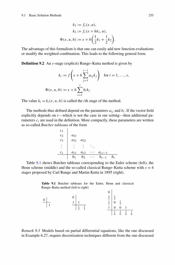
9.1 Basic Solution Methods 255
k1 := fc(x,u),
k2 := fc(x + hk1, u),
�(x,u,h) := x + h
(1
2k1 + 1
2k2
).
The advantage of this formalism is that one can easily add new function evaluationsor modify the weighted combination. This leads to the following general form.
Definition 9.2 An s-stage (explicit) Runge–Kutta method is given by
ki := f
(
x + h
i−1∑
j=1
aij kj
)
for i = 1, . . . , s,
�(x,u,h) := x + h
s∑
i=1
biki .
The value ki = ki(x,u,h) is called the ith stage of the method.
The methods thus defined depend on the parameters aij and bi . If the vector fieldexplicitly depends on t—which is not the case in our setting—then additional pa-rameters ci are used in the definition. More compactly, these parameters are writtenas so-called Butcher tableaus of the form
c1c2 a21c3 a31 a32...
......
. . .
cs as1 as2 · · · as s−1b1 b2 · · · bs−1 bs
Table 9.1 shows Butcher tableaus corresponding to the Euler scheme (left), theHeun scheme (middle) and the so-called classical Runge–Kutta scheme with s = 4stages proposed by Carl Runge and Martin Kutta in 1895 (right).
Table 9.1 Butcher tableaus for the Euler, Heun and classicalRunge–Kutta method (left to right)
0
1
0
1 112
12
012
12
12 0 1
2
1 0 0 116
26
26
16
Remark 9.3 Models based on partial differential equations, like the one discussedin Example 6.27, require discretization techniques different from the one discussed

256 9 Numerical Discretization
here. In particular, apart from the discretization in time also a discretization in spacehas to be performed. Popular techniques for this purpose are finite difference or fi-nite element methods and the interested reader is referred to the large amount oftextbooks on this topic, like, e.g., the books by LeVeque [9] or Braess [1], respec-tively.
9.2 Convergence Theory
Having defined one step methods we now show that the resulting approximationsactually converge towards the solution. To this end, we define the error at time τi ∈ Gas
e(τi) := ∥∥ϕ(τi; τ0, x,u) − ϕ(τi; τ0, x,u)∥∥.
The main idea to show convergence is to use the triangle inequality in order toseparate the error sources in the iteration (9.2) into the error caused by the previouslyaccumulated error (a) and the local error (b). Abbreviating ϕ(τi) = ϕ(τi; τ0, x0, u)
and ϕ(τi) = ϕ(τi; τ0, x0, u), this leads to the estimate
e(τi+1) = ∥∥ϕ(τi+1) − ϕ(τi+1)∥∥ = ∥∥�
(ϕ(τi), u,hi
) − ϕ(τi+1)∥∥
≤ ∥∥�(ϕ(τi), u,hi
) − �(ϕ(τi), u,hi
)∥∥︸ ︷︷ ︸
accumulated error (a)
+ ∥∥�(ϕ(τi), u,hi
) − ϕ(τi+1)∥∥
︸ ︷︷ ︸local error (b)
. (9.4)
The idea is sketched in Fig. 9.1 for i = 2.In order to prove convergence we will use the following conditions, which guar-
antee that both errors (a) and (b) remain small.
Definition 9.4
(i) A one step method satisfies the Lipschitz condition if for all compact subsetsK ⊂ R
d and Q ⊂ U there exists a constant � > 0 such that for all sufficientlysmall h > 0 the inequality
Fig. 9.1 Illustration of theseparation of errors

9.2 Convergence Theory 257
∥∥�(x1, u,h) − �(x2, u,h)∥∥ ≤ (1 + �h)‖x1 − x2‖ (9.5)
holds for all x1, x2 ∈ K and all u ∈ Q.(ii) A one step method is called consistent with order of consistency p > 0 if for
all compact subsets K ⊂ Rd and Q ⊂ U there exists a constant C > 0 such that
for all sufficiently small h > 0 the inequality∥∥�(x,u,h) − ϕ(h;0, x,u)
∥∥ ≤ Chp+1 (9.6)
holds for all x ∈ K and all u ∈ Q.
Inequality (9.5) guarantees that the propagation of previous errors within a onestep method, i.e., term (a), stays bounded. The consistency condition (9.6), on theother hand, ensures that the local error (b) remains small.
One can easily show that the previously introduced Euler approximation as wellas all explicit Runge–Kutta methods satisfy the Lipschitz condition (9.5) if the vec-tor field fc satisfies the Lipschitz condition from Assumption 2.4. The consistencycondition (9.6), on the other hand, cannot be checked that easily in general. In orderto verify that a method � exhibits an order of consistency p ≥ 1, one utilizes theTaylor approximation of the method with respect to the step size h in h = 0, i.e.
�(x,u,h) = x +p∑
i=1
hi
i!∂i
∂hi
∣∣∣∣h=0
�(x,u,h) + O(hp+1) (9.7)
and compares it to the Taylor approximation of the exact solution ϕ(h;0, x,u) withrespect to h in h = 0. It turns out that this Taylor approximation can be computedwithout actually using the—in general unknown—solution ϕ. To this end, we usethe higher order Lie derivative Li
fc, i ∈ N0, with respect to the vector field fc which
for arbitrary smooth vector fields g : Rd × U → R
d is defined inductively by
L0fc
g(x,u) = g(x,u), Lifc
g(x,u) =(
∂
∂xLi−1
fcg(x,u)
)fc(x,u).
Using the Lie derivative, the Taylor approximation of ϕ reads
ϕ(h;0, x,u) = x +p∑
i=1
hi
i! Li−1fc
fc(x,u) + O(hp+1). (9.8)
Then, if the p summands in (9.7) and (9.8) coincide, the scheme is consistent withorder p. In particular, if � can be written as
�(x,u,h) = x + hψ(x,u,h)
with a continuous function ψ satisfying ψ(x,u,0) = fc(x,u), then it follows thatthe order of consistency is at least p = 1.
Using this technique one can show that the order of consistency of the classicalRunge–Kutta method is p = 4. More generally, the comparison of the summandscan be used in order to derive conditions on the coefficients of arbitrary Runge–Kutta schemes for any consistency order p ≥ 1. Unfortunately, the number of these

258 9 Numerical Discretization
condition grows exponentially with p, hence for p ≥ 10 it is almost impossible touse them for constructing appropriate Runge–Kutta methods.
Note that in order to guarantee the order of consistency p the vector field fc needsto be p times continuously differentiable with respect to x in order to ensure thatapproximation (9.8) holds. If the vector field depends on t , then it also needs to bep times continuously differentiable with respect to t on the interval [τi, τi+1] if wewant to apply (9.6) on this interval. This is no problem as long as [τi, τi+1] ⊆ [0, T ],which is always the case in this section. However, if we consider sampled datasystems, i.e., (2.6) with v from (2.13) on an interval [τi, τi+1] with tn ∈ (τi, τi+1) forsome sampling time tn, this becomes a major issue since the control v and thus themap t �→ fc(x, v(t)) is in general discontinuous and thus in particular nonsmooth atthe sampling times. We will discuss this issue in Sect. 9.4, below.
After discussing the assumptions and how these assumptions can be checked, weare now ready to state the main result of this section.
Theorem 9.5 If a one step method � satisfies the Lipschitz condition (9.5) and theconsistency condition (9.6) with order p, then the approximation ϕ from (9.2) isconvergent in the sense of Definition 9.1(iii) with order of convergence p.
Proof We will show (9.1) for each grid G on [0, T ] with h > 0 sufficiently small.For simplicity of notation, we drop the index j in (9.1). To this end, fix two compactsets K ⊂ R
d and Q ⊂ U . Then the set
K1 := {ϕ(t;0, x0, u)
∣∣ t ∈ [0, T ], x0 ∈ K, u ∈ Q}
is again compact, since ϕ is continuous in all variables and images of compact setsunder continuous maps are again compact. We choose some δ > 0 and consider thecompact set
K2 := Bδ(K1) =⋃
x∈K1
Bδ(x),
which contains exactly those points x ∈ Rd which have a distance less or equal δ to
a point on a solution x(t;0, x0, u) with x0 ∈ K and u ∈ Q. Let � > 0 and C > 0be the constants in the Lipschitz condition (9.5) and the consistency condition (9.6),respectively, for K = K2 and the set Q fixed above.
We first prove (9.1) under the following condition, which we will verify after-wards.
For all grids G with sufficiently small h > 0, all initial
values x0 ∈ K and all u ∈ Q the grid function ϕ from
(9.2) satisfies ϕ(τi, τ0, x0, u) ∈ K2 for all τi ∈ G.
(9.9)
For proving (9.1) we choose x0 ∈ K and u ∈ Q and abbreviate ϕ(t) =ϕ(t; τ0, x0, u) and ϕ(τi) = ϕ(τi; τ0, x0, u). With
e(τi) := ∥∥ϕ(τi) − ϕ(τi)∥∥
we denote the error at time τi ∈ G . Then from (9.4) we obtain

9.2 Convergence Theory 259
e(τi+1) ≤ ∥∥�(ϕ(τi), u,hi
) − �(ϕ(τi), u,hi
)∥∥ + ∥∥�(ϕ(τi), u,hi
) − ϕ(τi+1)∥∥
≤ (1 + �hi−1)∥∥ϕ(τi−1) − ϕ(τi−1)
∥∥ + Chp+1i−1
= (1 + �hi−1)e(τi−1) + Chp+1i−1 ,
using (9.5) and (9.6) for K = K2 in the second inequality. These inequalities applysince the construction of K1 and K2 implies ϕ(τi) ∈ K1 ⊂ K2 and (9.9) ensuresϕ(τi) ∈ K2.
By induction over i we now show that this inequality implies the estimate
e(τi) ≤ Chp 1
�
(exp
(�(τi − τ0)
) − 1).
For i = 0 this inequality follows immediately. For i − 1 → i we use
exp(�hi) = 1 + �hi + �2h2i
2+ · · · ≥ 1 + �hi,
which together with the induction assumption yields
e(τi) ≤ (1 + �hi−1)e(τi−1) + Chp+1i−1
≤ (1 + �hi−1)Chp 1
�
(exp
(�(τi−1 − τ0)
) − 1) + hi−1 Ch
p
i−1︸ ︷︷ ︸≤Ch
p
= Chp 1
�
(hi−1� + (1 + �hi−1)
(exp
(�(τi−1 − τ0)
) − 1))
= Chp 1
�
(hi−1� + (1 + �hi−1) exp
(�(τi−1 − τ0)
) − 1 − �hi−1)
= Chp 1
�
((1 + �hi−1) exp
(�(τi−1 − τ0)
) − 1)
≤ Chp 1
�
(exp(�hi−1) exp
(�(τi−1 − τ0)
) − 1)
= Chp 1
�
(exp
(�(τi − τ0)
) − 1).
Since τ0 = 0 this implies (9.1) with M = C(exp(�T ) − 1)/�.It remains to show that assumption (9.9) is satisfied. We show that this assump-
tion holds for all grids G whose maximal step size satisfies
Chp ≤ δ�
exp(�(T − τ0)) − 1.
To this end, we consider a numerical solution ϕ(τi) = ϕ(τi , τ0, x0, u) for some x0 ∈K and u ∈ Q and show ϕ(τi) ∈ K2 by induction. Since ϕ(τ0) = x0 ∈ K ⊂ K2 theassertion holds for i = 0.
For the induction step i − 1 → i assume that the induction assumption ϕ(τk) ∈K2 holds for k = 0,1, . . . , i − 1. We have to show ϕ(τi) ∈ K2. Observe that for theinequality
e(τi) ≤ Chp 1
�
(exp
(�(T − τ0)
) − 1)

260 9 Numerical Discretization
to hold it is sufficient that ϕ(τk) ∈ K2 holds for k = 0,1, . . . , i − 1. By choice of h
we thus obtain e(τi) ≤ δ, i.e.,∥∥ϕ(τi) − ϕ(τi)
∥∥ ≤ δ.
Since by construction of K1 we have ϕ(τi) ∈ K1, it follows that ϕ(τi) ∈ Bδ(ϕ(τi)) ⊂K2, i.e., the desired property. �
9.3 Adaptive Step Size Control
The convergence theorem from the previous section shows that the presented onestep methods are applicable to solve the underlying continuous time dynamics of theform (2.6) of a problem (OCPn
N,e). Yet, so far we can only guarantee those methodsto exhibit small errors if each time step hi in the grid G is sufficiently small sincethe error bound in (9.1) depends on h = maxhi . In the literature, it is occasionallyproposed to use the grid induced by the sampling times as computational grid, i.e.,to choose τn = tn = nT . This, however, results in h = T and thus requires the sam-pling period T to be small in order to obtain an accurate approximation. Apart fromthe fact that it may not be desirable to use very small sampling periods, there aresubtle pitfalls regarding stability of the closed-loop system when the accuracy of theapproximate model and the sampling rate are linked, see the discussion in Sect. 9.6.
A way to avoid linking h and T is to use a constant step size hi ≡ h withh = T/K for some K ∈ N. Adjusting h appropriately, we can make the error termin (9.1) arbitrarily small without changing T . This, however, leads to equidistantgrids, which are known to be computationally inefficient since they do not reflectthe properties of the solution. A much more efficient way is to choose the time stepshi adapted to the solution, i.e., we allow for large hi if the error is small and usesmall hi when large errors are observed. However, we surely do not want to manu-ally adapt the step sizes to every situation the NMPC controller may face since thiswould render such an algorithm to be inapplicable.
In order to obtain an efficient way to construct an adaptive grid G , we considerstep size control algorithms. Such methods are well established in the numerics ofordinary differential equations. In this section we explain the central idea behindstep size control algorithms. The key idea is to use two different one step methods�1, �2 with different orders of consistency p1 < p2 in order to compute a steplength hi = τi+1 − τi at time τi for the next time step which guarantees a prede-fined local error bound tolODE. Here, by p1 < p2 we mean that for � = �1 theInequality (9.6) cannot hold for p = p2, i.e., no matter how C is chosen (9.6) willbe violated for all sufficiently small h. As in the previous sections, we consider thesolution of (2.6) on one sampling interval [0, T ] on which the control u is constant.
In (9.4) we used the auxiliary term �(ϕ(τi; τ0, x,u),u,hi) in order to quantifythe local error. Since the value of ϕ(τi;0, x,u) is not available at runtime of a onestep method, we cannot use it to guarantee the local error (a) to satisfy
∥∥�
(ϕ(τi; τ0, x,u),u,hi
) − ϕ(τi; τ0, x,u)∥∥ ≤ tolODE.

9.3 Adaptive Step Size Control 261
To circumvent this problem, in the triangle inequality for estimating e(τi+1) we in-sert the term ϕ(τi+1; τi, ϕ(τi; τ0, x,u),u) instead of �(ϕ(τi; τ0, x,u),u,hi). Usingthat by the cocycle property we have ϕ(τi+1; τ0, x,u) = ϕ(τi+1; τi, ϕ(τi; τ0, x,u),
u), this leads to the inequality∥∥ϕ(τi+1; τ0, x,u) − ϕ(τi+1; τ0, x,u)
∥∥
≤ ∥∥�(ϕ(τi; τ0, x,u),u,hi
) − ϕ(τi+1; τi, ϕ(τi; τ0, x,u),u
)∥∥
+ ∥∥ϕ(τi+1; τi, ϕ(τi; τ0, x,u),u
) − ϕ(τi+1; τi, ϕ(τi; τ0, x,u),u
)∥∥.
In this sum the second term essentially depends on the error of the approximationat time instant τi , which is independent of the choice of hi = τi+1 − τi . Hence,for choosing hi we only consider the first summand. More precisely, we attempt tochoose hi such that the tolerable error bound
∥∥�(ϕ(τi; τ0, x,u),u,hi
) − ϕ(τi+1; ti, ϕ(τi; τ0, x,u),u
)∥∥ ≤ tolODE
is satisfied.When trying to implement this method, one faces the problem that the value
ϕ(τi+1; ti , ϕ(τi; τ0, x,u),u) is not known. This is where the idea of using two meth-ods �1 and �2 with different orders of consistency p2 > p1 is used. Setting � = �1and approximating ϕ(τi+1; ti , ϕ(τi; τ0, x,u),u) by the more accurate method �2one can show the following theorem.
Theorem 9.6 Consider two one step methods �1, �2 with orders of consistencyp1, p2 satisfying p2 ≥ p1 + 1. Then there exist constants k1, k2 > 0 such that for allsufficiently small hi > 0 the computable error
ε := ∥∥�1(ϕ(τi;0, x,u),u,hi
) − �2(ϕ(τi;0, x,u),u,hi
)∥∥ (9.10)
and the local error of the one step method �1
ε := ∥∥�1(ϕ(τi;0, x,u),u,hi
) − ϕ(τi+1; τi, ϕ(τi;0, x,u),u
)∥∥
satisfy the inequality
k1ε ≤ ε ≤ k2ε.
Proof First we define the errors
ηi,j := �j
(ϕ(τi;0, x,u),u,hi
) − ϕ(τi+1; τi, ϕ(τi;0, x,u),u
)
for both one step methods �j , j = 1,2. By Definition 9.4(ii) we obtain the local
error bounds εi,j := ‖ηi,j‖ ≤ Cjhpj +1i . Using p2 ≥ p1 + 1 and the fact that this im-
plies εi,1 ≥ Chp2+1i for all C > 0 and all sufficiently small hi > 0, we can conclude
θ := εi,2/εi,1 < 1 if hi is chosen sufficiently small since θ → 0 as hi → 0. We fixθ0 < 1, consider hi > 0 such that θ < θ0 < 1 holds and define
η := �1(ϕ(τi;0, x,u),u,hi
) − �2(ϕ(τi;0, x,u),u,hi
) = ηi,1 − ηi,2.
Then we have

262 9 Numerical Discretization
(1 − θ)εi,1 = (1 − θ)‖ηi,1‖ =(
1 − ‖ηi,1 − η‖‖ηi,1‖
)‖ηi,1‖
= ‖ηi,1‖ − ‖ηi,1 − η‖ ≤ ‖η‖ = ε,
which yields the lower bound k1 = 1 − θ0 and
ε = ‖η‖ ≤ ‖ηi,1‖ + ‖ηi,1 − η‖ =(
1 + ‖ηi,1 − η‖‖ηi,1‖
)‖ηi,1‖
= (1 + θ)‖ηi,1‖ = (1 + θ)εi,1
giving the upper bound k2 = 1 + θ0. �
Using Theorem 9.6 we can now compute a suitable step size hi if we additionallyassume that the local error is of the form εi,1 ≈ cih
p1+1i for small hi . Note that for
Runge–Kutta methods this assumption is satisfied if the vector field f is p1 + 2times continuously differentiable. In this case, ci is given by the coefficient of theh
p1+1i term in the Taylor approximation of the method.
For small step sizes it follows from the proof of Theorem 9.6 that k1 ≈ k2 ≈ 1,i.e. ε ≈ εi,1 ≈ cih
p1+1i , which gives us the estimate ci ≈ ε/h
p1+1i for the coefficient
ci . Hence, the error tolerance tolODE is satisfied (approximately) for the step size
tolODE = cihp1+1i,new = ε
hp1+1i
hp1+1i,new ⇐⇒ hi,new = p1+1
√
factolODE
εhi . (9.11)
Since all these equalities are only satisfied approximately, a security factor fac ∈(0,1) has been introduced to compensate for these approximation errors. For thisfactor, fac = 0.9 is a typical choice in many algorithms.
A schematic implementation of a one step scheme with adaptive step size isgiven in Algorithm 9.7, below. This algorithm combines the iteration (9.2) withthe computation of the step size hi described above. Here we solve (2.6) on onesampling interval [0, T ] using the length T of the sampling interval as an initialchoice for the first step size h0. For large T , one may alternatively choose h0 < T .In each step the error ε is computed. If ε exceeds the tolerance tolODE, then thestep is rejected and repeated using the new step size from (9.11). If ε maintains thedesired tolerance, then the step is accepted and the new step size from (9.11) is usedas an initial choice for the next time step.
Algorithm 9.7 Suppose an initial value x, a control value u, a tolerance tolODE
and sampling period T are given.
(1) Set ϕ(0;0, x, v) = x, i = 0, τ0 = 0, h0 = T
(2) If τi = T stop; If τi + hi > T set hi = T − τi
(3) Set τi+1 = τi + hi and compute �1(ϕ(τi+1; tj , x, u),u,hi), �2(ϕ(τi+1; tj ,x, u),u,hi)
(4) Compute ε and hi,new according to (9.10), (9.11)(5) If ε > tolODE set hi = hi,new and goto (3)

9.3 Adaptive Step Size Control 263
Table 9.2 Butcher tableau of the DoPri(4)5 method
0
15
15
310
340
940
45
4445 − 56
15329
89
19 3726561 − 25 360
218764 4486561 − 212
729
1 90173168 − 355
3346 7325247
49176 − 5103
18 656
1 35384 0 500
1113125192 − 2187
67841185
35384 0 500
1113125192 − 2187
67841184 0
517957 600 0 7571
16 695393640 − 92 097
339 200187
2100140
(6) If ε ≤ tolODE set ϕ(τi+1; τ0, x,u) = �2(ϕ(τi+1; τ0, x,u),u,hi), hi+1 = hi,new,i = i + 1 and goto (2)
In practical implementations, this basic algorithm is often refined in variousways. For instance, the new step size may be derived on the basis of a weightedsum of the absolute and the relative error instead of using only the absolute error asabove. Upper and lower bounds for the time step hi as well as for the ratio betweenhi and hi+1 are also frequently used in practice.
Although the evaluation of two methods �1 and �2 and their possibly repeatedevaluation in every step seems to be computationally more demanding, step sizecontrol algorithms are usually much more efficient than the use of equidistant timegrids. This is due to two different aspects: on the one hand, there typically existregions which allow for larger time steps and thus allow for a faster progress ofthe adaptive iteration procedure. On the other hand, the additional effort of simul-taneously evaluating two methods can be reduced significantly by embedding thesemethods into each other. This means that the less accurate Runge–Kutta method �1uses the same stages ki , cf. Definition 9.2, as the more accurate methods �2 andthus the stages ki only need to be evaluated once for both methods. One standardembedded method is the Dormand–Prince method of order (4)5, also called DoPri5,in which �1 has order p1 = 4 and �2 is of order p2 = 5. The Butcher tableau isdisplayed in Table 9.2. The second last line specifies the coefficients bi for �1 andthe last line the bi for �2.
With the same induction as in the proof of Theorem 9.5, one sees that if thelocal errors maintain the tolerances tolODE = εhi for some ε > 0, then the overallerror at time T can be estimated as e(T ) ≤ ε(exp(�T ) − 1)/� and thus scaleslinearly with ε. It should, however, be mentioned that adaptive step size selectionschemes usually do not rigorously maintain the specified error tolerance. The reasonfor this is that Theorem 9.6 and the derivation of (9.11) require hi to be sufficientlysmall. Suitable upper bounds which quantify this “sufficiently small” are, however,

264 9 Numerical Discretization
difficult to obtain without an extensive a priori analysis of the individual system andcan therefore not be enforced in practice. Hence, the step size selection algorithmmay select large step sizes for which the error estimation is no longer valid and thusthe desired accuracy is no longer guaranteed. Thus, in general only equidistant gridswith sufficiently small maximal step size h provide rigorous error bounds. Still,numerical experience shows that in the vast majority of examples error estimationbased adaptive step size algorithms like Algorithm 9.7 perform very reliably.
9.4 Using the Methods Within the NMPC Algorithms
Looking at the NMPC Algorithm 3.11 and its variants, we see that in every iterationan optimal control problem (OCPn
N,e) has to be solved. To this end, the optimizationalgorithm needs to be able to compute the solution xu and to evaluate the functionalJN . In fact, there are various ways for incorporating xu into the optimization algo-rithm, for details see Sect. 10.1. However, no matter which method from this sectionwe use, we need to be able to evaluate ϕ(T ,0, x,u) in (2.8) numerically.
To this end, we replace the unknown map ϕ(T ,0, x,u) in (2.8) by its approxima-tion ϕ(T ,0, x,u) from Algorithm 9.7. This way we end up with the definition
x+ = f (x,u) := ϕ(T ,0, x,u). (9.12)
Iterating this map according to (2.2), which amounts to calling Algorithm 9.7 N
times with initial values xu(n, x) and control values u(n), n = 0, . . . ,N − 1, wecan then obtain an approximate predicted solution trajectory. Proceeding this way,one should keep in mind that the numerical scheme provides only an approximationof the exact solution. The effects of the approximation errors will be discussed inSect. 9.5, below.
When the running cost � is defined via the integral formula (3.4), then we canefficiently include the numerical evaluation of the integral
�(x,u) =∫ T
0L
(ϕ(t,0, x,u),u
)dt
into the computation of ϕ. Here we have removed the argument t from u because—following the convention in this chapter—u is constant on the sampling interval[0, T ]. In order to compute the integral, consider the augmented ordinary differentialequation
x(t) = f(x(t), u
)(9.13)
with
x(t) =(
x(t)
y(t)
)∈ R
d × R and f (x,u) =(
fc(x,u)
L(x,u)
).
Solving (9.13) with initial condition x = (x,0) we obtain the solution
ϕ(T , x,u) =(
ϕ(T , x,u)
�(x,u)
).
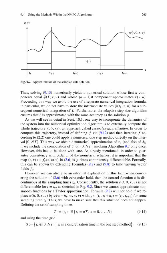
9.4 Using the Methods Within the NMPC Algorithms 265
Fig. 9.2 Approximation of the sampled data solution
Thus, solving (9.13) numerically yields a numerical solution whose first n com-ponents equal ϕ(T , x,u) and whose (n + 1)st component approximates �(x,u).Proceeding this way we avoid the use of a separate numerical integration formula,in particular, we do not have to store the intermediate values ϕ(τi , x, u) for a sub-sequent numerical integration of L. Furthermore, the adaptive step size algorithmensures that � is approximated with the same accuracy as the solution ϕ.
As we will see in detail in Sect. 10.1, one way to incorporate the dynamics ofthe system into the numerical optimization algorithm is to externally compute thewhole trajectory xu(·, x0), an approach called recursive discretization. In order tocompute this trajectory, instead of defining f via (9.12) and then iterating f ac-cording to (2.2) one could apply a numerical one step method directly on the inter-val [0,NT ]. This way we obtain a numerical approximation of xu (and also of JN
if we include the computation of �) on [0,NT ] invoking Algorithm 9.7 only once.However, this has to be done with care. As already mentioned, in order to guar-antee consistency with order p of the numerical schemes, it is important that themap (t, x) �→ fc(x, v(t)) in (2.6) is p times continuously differentiable. Formally,this can be shown by extending Formulas (9.7) and (9.8) to time varying vectorfields fc .
However, we can also give an informal explanation of this fact: when consid-ering the solution of (2.6) with zero order hold, then the control function v is dis-continuous at the sampling times tn. Consequently, the solution ϕ(t,0, x, v) is notdifferentiable for t = tn, as sketched in Fig. 9.2. Since we cannot approximate non-smooth functions by a Taylor approximation, Formula (9.8) will not hold if we re-place ϕ(h,0, x,u) by ϕ(τi +hi, τi, x, v) with tn ∈ (τi, τi +hi) = (τi, τi+1) for somesampling time tn. Thus, we have to make sure that this situation does not happen.Defining the set of sampling times
T := {tn ∈ R | tn = nT , n = 0, . . . ,N} (9.14)
and using the time grid
G := {τi ∈ [0,NT ] ∣
∣ τi is a discretization time in the one step method}, (9.15)

266 9 Numerical Discretization
in order to exclude the existence of i and n with tn ∈ (τi, τi + hi) = (τi, τi+1) weneed to make sure that the inclusion T ⊂ G holds. This assumption is not veryrestrictive, however, in order to ensure it we need to appropriately adjust Algo-rithm 9.7.
9.5 Numerical Approximation Errors and Stability
Defining the discrete dynamics f via the numerical approximation ϕ, cf. (9.12),introduces errors in the predictions xu in the optimal control problems (OCPn
N,e)and its variants. In this section we shift our focus from analyzing the effects of theseerrors on the open loop towards their effect on the closed loop. To this end, weutilize the techniques from Sects. 8.5–8.9 and—similar to these sections—restrictourselves to constant reference x ref ≡ x∗ in order to simplify the exposition. For theextension to time varying xref we refer to the remarks following the main results inSects. 8.5–8.9.
As a general assumption we suppose that for each ε > 0 we can compute a nu-merical approximation ϕε which satisfies
∥∥ϕε(T ,0, x,u) − ϕ(T ,0, x,u)∥∥ ≤ ε (9.16)
for some ε > 0, all x ∈ X and u ∈ U(x). As discussed at the end of Sect. 9.3, such anestimate is rigorously ensured for ϕε generated by one step methods on equidistantgrids with sufficiently small h > 0 but can typically also be expected for ϕ from theadaptive step size Algorithm 9.7 by adjusting the tolerance tolODE appropriately.Observe that since (9.1) only holds for x and u from compact sets, in the caseof equidistant grids we may have to adjust h > 0 to x and u in order to ensure(9.16) if X or U(x) are noncompact. In case of Algorithm 9.7 the step size will beautomatically adjusted by the step size selection mechanism.
Given that ϕε is an approximation of the true solution ϕ it seems natural to con-sider ϕε as a perturbed version of ϕ. However, since by definition the model used inthe NMPC algorithm—i.e., the numerical approximation ϕε—is the nominal model,we need the converse interpretation in order to apply the results from Sects. 8.5–8.9.In what follows we show that the closed loop obtained from the exact sampled datasystem (2.8) can be considered as a perturbed system in the sense of Sect. 8.5. Tothis end, we consider the following setting.
The NMPC algorithm is run with the numerically approximated discrete dynam-ics
f (x,u) = f ε(x,u) := ϕε(T ,0, x,u) (9.17)
as a nominal model. The resulting NMPC-feedback law is denoted by μεN . With
xεμε
Nand xε
μεN
we denote the corresponding nominal and perturbed NMPC closed-
loop trajectory from (3.5) and (8.7) with f = f ε = ϕε and μN = μεN , respectively,
i.e.,
xεμε
N(n + 1) = f ε
(xεμε
N(n),με
N
(xεμε
N(n)
))

9.5 Numerical Approximation Errors and Stability 267
and
xεμε
N(n + 1) = f ε
(xεμε
N(n),με
N
(xεμε
N(n) + e(n)
)) + d(n).
The closed-loop system obtained from applying the numerically computed NMPCfeedback με
N to the exact model f = ϕ from (2.8) according to (3.5), i.e.,
xexμε
N(n + 1) = f
(xexμε
N(n),με
N
(xexμε
N(n)
)),
will be called the exact closed-loop system. The resulting trajectories will be denotedby xex
μεN
.
Note that the same NMPC-feedback law μεN —computed from f = f ε = ϕε—is
used in (3.5) for generating xεμε
Nand xex
μεN
. The difference between the two trajecto-
ries only lies in the map f in (3.5), which is given by f = f ε = ϕε for xεμε
Nand by
f = ϕ for xexμε
N. Using this notation we obtain the following result.
Lemma 9.8 Consider the discrete time dynamics f = f ε from (9.17) obtained froma numerical approximation ϕε satisfying (9.16), an NMPC-feedback law με
N withμε
N(x) ∈ U(x) and the solution xεμε
Nof the corresponding closed-loop system (3.5).
Consider, furthermore, the solution xexμε
Nof the exact closed-loop system.
Then for each x0 ∈ X there exists a perturbation sequence d(·) ∈ (Rd)∞ with‖d(n)‖ ≤ ε such that the solution xε
μεN(n, x0) of the perturbed system (8.7) with
f = f ε and e ≡ 0 satisfies
xexμε
N(n, x0) = xε
μεN(n, x0)
for all n ∈ N0.
Proof Define
d(n) := ϕ(T ,0, xex
μεN(n, x0),μ
εN
(xexμε
N(n, x0)
))
− ϕε(T ,0, xex
μεN(n, x0),μ
εN
(xexμε
N(n, x0)
))
for all n ∈ N0. Then (9.16) with x = xexμε
N(n, x0) and u = με
N(xexμε
N(n, x0)) implies
‖d(n)‖ ≤ ε for all n ∈ N0. We show the desired identity by induction over n. For n =0 we obtain xex
μεN(0, x0) = x0 = xε
μεN(0, x0). For n → n+1 assume that xex
μεN(n, x0) =
xεμε
N(n, x0) holds. Then we get
xexμε
N(n + 1, x0) = ϕ
(T ,0, xex
μεN(n, x0),μ
εN
(xexμε
N(n, x0)
))
= ϕε(T ,0, xex
μεN(n, x0),μ
εN
(xexμε
N(n, x0)
)) + d(n)
= f ε(xexμε
N(n, x0),μ
εN
(xexμε
N(n, x0)
)) + d(n)
= f ε(xεμε
N(n, x0),μ
εN
(xεμε
N(n, x0)
)) + d(n)
= xεμε
N(n + 1, x0).
This shows the assertion. �

268 9 Numerical Discretization
Lemma 9.8 shows that the closed-loop solution for the discrete time model ob-tained from the exact sampled data system (2.8) can be interpreted as a perturbed so-lution of the discrete time model obtained from the numerical approximation (9.17).The size of the perturbation d(·) directly corresponds to the numerical error (9.16).
This lemma enables us to use all results from Sects. 8.5–8.9 in order to con-clude stability properties for xex
μεN
. The appropriate stability property is given by the
following definition, cf. Definition 8.24.
Definition 9.9 Consider the exact closed-loop system (2.5) with f = ϕ from (2.8)with με
N computed from f = f ε = ϕε from (9.17) satisfying (9.16) for some ε > 0.Given a set A ⊆ X such that the optimal control problem defining με
N is feasiblefor all x0 ∈ A, we say that x∗ is semiglobally practically asymptotically stable on A
with respect to the numerical error ε if there exists β ∈ K L such that the followingproperty holds: for each δ > 0 and � > δ there exists ε > 0, such that for each initialvalue x0 ∈ A with |x0|x∗ ≤ � and each ε ∈ (0, ε] the solution xex
μεN(·, x0) satisfies
xexμε
N(k, x0) ∈ A and
∣∣xexμε
N(k, x0)
∣∣x∗ ≤ max
{β(|x0|x∗, k
), δ
}
for all k ∈ N0.
The following theorem now gives conditions under which this stability propertyholds.
Theorem 9.10 Consider the NMPC-feedback laws μεN obtained from one of the
NMPC algorithms from Theorem 8.26, 8.36 or 8.41 with f = f ε = ϕε from (9.17).Assume that (9.16) holds and that there is ε0 > 0 such that one of the followingassumptions is satisfied for all ε ∈ (0, ε0].
(i) In case of Theorem 8.26, assume that α, α1, α2, α3 in Theorem 4.11 as well asωV and ωf can be chosen independently of ε > 0.
(ii) In case of Theorem 8.36, assume that α, α1, α in Theorem 6.18, β from As-sumption 8.35 and η in Definition 8.33 can be chosen independently of ε > 0.
(iii) In case of Theorem 8.41, assume that α, α1, α2, α3 in Theorem 4.11, δ, γ , ε′ inAssumption 8.38 and the bound on f as well as the moduli of continuity of f
and � can be chosen independently of ε > 0.
Then the exact closed-loop system (2.5) with f = ϕ from (2.8) is semigloballypractically asymptotically stable with respect to ε from (9.16) in the sense of Defi-nition 9.9 on the set A specified in the respective theorem.
Proof The respective theorems ensure semiglobal practical asymptotic stability forall perturbed trajectories xε
μεN
with respect to d and e in the sense of Definition 8.24.
An inspection of the proofs of the respective theorems then reveals that the unifor-mity assumptions (i)–(iii) guarantee that for given δ and � the bounds d and e andthe function β ∈ K L in Definition 8.24 are independent of ε > 0.

9.6 Notes and Extensions 269
Fixing δ and � we thus find d > 0 such that each perturbed solution xεμε
Nwith
perturbations ‖d(n)‖ ≤ d and e ≡ 0 satisfies the conditions of Definition 8.24 for allε ∈ (0, ε0]. Setting ε = min{d, ε0} and using that by Lemma 9.8 the exact closed-loop trajectory xex
μεN
equals one of the trajectories xεμε
Nwith d = ε and e = 0, we
obtain that xexμε
Nsatisfies the conditions of Definition 9.9 for the given δ and � and
all ε ∈ (0, ε]. This yields the assertion. �
Note that Theorem 9.10 only guarantees the stability of the discrete time closed-loop system (2.5) with f from (2.8) but not for the sampled data closed loop (2.30).In order to conclude stability properties of (2.30) the techniques from Sect. 2.4can be used. While Theorem 2.27 and its assumptions are formulated for the caseof “real” asymptotic stability, its statement and proof can be straightforwardly ex-tended to the semiglobal practical setting of Definition 9.9. Recall from Remark 4.13that the assumptions of Theorem 2.27 are satisfied for suitable integral costs (3.4).Although we have not rigorously analyzed the effect of the error induced by thenumerical approximation of such integral costs, we conjecture that the estimates inRemark 4.13 remain valid in a suitable approximate sense if these errors are suffi-ciently small.
Since numerical approximations are used in virtually all NMPC algorithms forsampled data systems, Theorem 9.10 implies that all such algorithms need appro-priate robustness—either inherently as in case (i) or by an appropriate design ofthe state constraints as in cases (ii) and (iii) of Theorem 9.10—in a uniform waywith respect to ε in order to ensure semiglobal practical stability in the presence ofnumerical errors. In practice, however, this is hardly ever rigorously ensured. Thereason for this is that for good numerical methods numerical errors are usually verysmall compared to other error sources like model errors, external perturbations etc.Although even very small errors may in the worst case be destabilizing, as illus-trated by Example 8.31, it is not very likely that this indeed happens and—alsoaccording to our experience—such phenomena are hardly ever observed in simula-tions or practical examples. Hence, unless robustness is needed in order to cope witherror sources which are significantly larger than the numerical errors discussed inthis chapter, for most practical purposes it seems justified to neglect the robustnessissue, provided, of course, the numerical errors are indeed sufficiently small. Still,one has to keep in mind that proceeding this way does not rigorously ensure stabilityof the exact closed-loop system.
9.6 Notes and Extensions
The material contained in Sects. 9.1–9.3 can be found in many textbooks on numeri-cal analysis for ordinary differential equations, like, e.g., the books by Deuflhard andBornemann [2], Hairer, Nørsett and Wanner [8] or Stoer and Bulirsch [11]. Clearly,the presentation in this chapter cannot replace any of these textbooks and aims atgiving an introduction into the subject rather than a comprehensive treatment.

270 9 Numerical Discretization
Among the many topics we have not covered in this chapter we would in par-ticular like to mention stiff problems and differential algebraic equations (DAEs),often called descriptor systems in systems theory. While stiff problems “look” likenormal ordinary differential equations, they are very difficult to solve with the ex-plicit methods presented in Sect. 9.1. For stiff equations, which often appear whenmodeling technical systems, an adaptive step size algorithm like Algorithm 9.7 willtypically select very small time steps even though the solution is almost constant.Explaining the precise mathematical reasons for this behavior goes beyond thesenotes, but we would at least like to mention that so-called implicit methods performmuch better for stiff equations. DAEs are ordinary differential equations with ad-ditional algebraic constraints, often given implicitly. DAEs appear as models, e.g.,in mechanics and electrical engineering and NMPC is perfectly suited for handlingDAEs, however, the solution methods presented in this chapter do not apply to suchequations and specialized numerical schemes are needed, which are again often ofthe implicit type. While also covered in some standard textbooks, there is a largeamount of literature particularly devoted to stiff and DAE problems, as, e.g., Hairerand Wanner [7], and we refer the reader to such books for more details.
As Examples 2.12 and 6.27 show, NMPC is also suitable for infinite-dimensionalsystems generated by controlled PDEs. NMPC for PDEs requires the solution of anoptimal control problem for PDEs in each step. The monograph by Tröltzsch [12]provides a good introduction into such problems. A simple way to approach thisproblem numerically is to proceed similar as described for the ordinary differentialequations in this chapter with an additional spatial discretization by, e.g., a finitedifference method (which is what we used in Example 6.27), see, e.g., LeVeque[9] or a finite element method, see, e.g., Braess [1]. However, it is by no meansclear whether this is the most efficient way of approaching the problem numerically;in fact, the development of suitable numerical schemes is currently a very activeresearch area. Furthermore, we are not aware of a rigorous analysis of the effects ofspatial discretization errors in NMPC controller design.
The need to use numerical approximations and the consequences for the stabil-ity analysis discussed in Sect. 9.5 are largely ignored in the NMPC literature. Anexception to this rule are the papers by Gyurkovics and Elaiw [5, 6], which are inthe same spirit as cases (i) and (iii) of Theorem 9.10 in the sense that they exploituniform continuity properties, in particular of the optimal value function VN . How-ever, these results require Lyapunov function terminal costs and do not considerstate constraints as in cases (ii) and (iii) of Theorem 9.10.
More generally, the problem considered in Sect. 9.5 can be seen as a special caseof a nonlinear controller design based on approximate models. A comprehensivetreatment of this topic in a rather general setting can be found in Nešic and Teel[10]. An application to infinite horizon optimal control based feedback design wasgiven in Grüne and Nešic [4]. The idea to treat numerical errors as perturbationsis classical in numerical analysis. In a control theoretic framework this idea wasused extensively in the monograph Grüne [3]. All these approaches are similar toour approach in the sense that the stability property of the approximate system isrequired to be robust in some suitable sense, that the robustness can be quantified

9.7 Problems 271
and that this quantitative measure of the robustness is independent of the numericalaccuracy. In all cases the obtained stability property is semiglobal practical stability,just as in Theorem 9.10. State constraints are, however, again not considered in thesereferences.
Nešic and Teel [10] also nicely illustrate the pitfalls of feedback design based onapproximate models by means of simple examples and discuss the case in which thenumerical accuracy is linked to the sampling period T . Roughly speaking, in thiscase uniform continuity of the Lyapunov function under consideration is not suffi-cient in order to ensure stability of the exact closed-loop system. Rather, a strongerproperty like Lipschitz continuity with Lipschitz constant independent of the nu-merical accuracy ε is needed in this case.
There are numerous issues related to numerical errors we have not addressedin this chapter. For instance, numerical errors may lead to the situation that theinequalities in Assumption 5.9(ii) or Assumption 6.4 are only satisfied up to anerror term ε, which has to be taken into account in the results relying on theseassumptions. While we conjecture that in both cases the respective proofs can bemodified in order to obtain at least semiglobal practical asymptotic stability of xε
μεn,
we are not aware of respective results in the literature. Hence, this area certainlyoffers a number of open questions for future research.
9.7 Problems
1. Prove that the solution ϕ(t,0, x0, u) of (2.6) with t ∈ [0, T ] and constant controlfunction u satisfies the integral equation
ϕ(τi+1; τ0, x0, u) = ϕ(τi; τ0, x0, u) +∫ τi+1
τi
fc
(ϕ(t; τ0, x0, u), u
)dt
for all τi, τi+1 ∈ [0, T ] with τi+1 > τi .2. Prove that the Euler and the Heun scheme satisfy the Lipschitz condition (9.5) if
the vector field fc satisfies the Lipschitz condition from Assumption 2.4.3. Given the control system x(t) = x(t)+u(t) with running cost �(x,u) = x2 +u2.
(a) Consider the NMPC Algorithm 3.1 with N = 2 and f generated by the Eu-ler method with G = T for (9.14) and (9.15). Prove that the control μN(x)
converges to zero as T → 0 for each x ∈ R.(b) Consider the same situation as in (a) but with the grid
G := {τi = iT /k | i = 0, . . . ,Nk}with k ∈ N. Does the control value μN(x) converge if T > 0 is fixed and k
tends to infinity?4. Consider the differential equation
x1(t) = −x2(t),
x2(t) = x1(t)
272 9 Numerical Discretization
whose solution shall be used to generate a time varying reference xref for anNMPC algorithm.(a) Using a transformation to polar coordinates, compute the analytical solution
of the system.(b) Show that the numerical solution of the system using Euler’s method will
deviate from the analytical solution from (a) for every step size h > 0 andevery initial value x0 �= (0,0)�.
(c) Applying the transformation to polar coordinates, show that the occurringerror from (b) can be avoided if the resulting differential equation is solvedusing Euler’s method.
5. Consider the continuous time control system
x1(t) = −x2(t) + v(t),
x2(t) = x1(t)
where u shall be computed via NMPC to track the (exact) time varying referencesolution from Problem 4 with initial value x0 �= 0.(a) Show that this system is (uniformly) asymptotically controllable in the sense
of Definition 4.2 for control functions which are piecewise constant on eachinterval [iT , (i + 1)T ) for arbitrary sampling time T > 0 which is not aninteger multiple of π .
(b) Consider the approximate discrete time system (9.12) with ϕ obtained fromapplying the Euler method with step size h = T to the (nontransformed) dif-ferential equation. Show that this approximate system is not asymptoticallycontrollable for any T > 0 as in (a).
Hint for (b): A necessary condition for asymptotic controllability is that the ref-erence x ref is a solution of the system.
References
1. Braess, D.: Finite Elements, 3rd edn. Cambridge University Press, Cambridge (2007). Theory,Fast Solvers, and Applications in Elasticity Theory. Translated from the German by Larry L.Schumaker
2. Deuflhard, P., Bornemann, F.: Scientific Computing with Ordinary Differential Equations.Texts in Applied Mathematics, vol. 42. Springer, New York (2002). Translated from the 1994German original by Werner C. Rheinboldt
3. Grüne, L.: Asymptotic Behavior of Dynamical and Control Systems Under Perturbation andDiscretization. Lecture Notes in Mathematics, vol. 1783. Springer, Berlin (2002)
4. Grüne, L., Nešic, D.: Optimization based stabilization of sampled-data nonlinear systems viatheir approximate discrete-time models. SIAM J. Control Optim. 42, 98–122 (2003)
5. Gyurkovics, E., Elaiw, A.M.: Stabilization of sampled-data nonlinear systems by recedinghorizon control via discrete-time approximations. Automatica 40(12), 2017–2028 (2004)
6. Gyurkovics, E., Elaiw, A.M.: Conditions for MPC based stabilization of sampled-data nonlin-ear systems via discrete-time approximations. In: Findeisen, R., Allgöwer, F., Biegler, L.T.(eds.) Assessment and Future Directions of Nonlinear Model Predictive Control. LectureNotes in Control and Information Sciences, vol. 358, pp. 35–48. Springer, Berlin (2007)

References 273
7. Hairer, E., Wanner, G.: Solving Ordinary Differential Equations. II, 2nd edn. Springer Seriesin Computational Mathematics, vol. 14. Springer, Berlin (1996)
8. Hairer, E., Nørsett, S.P., Wanner, G.: Solving Ordinary Differential Equations. I, 2nd edn.Springer Series in Computational Mathematics, vol. 8. Springer, Berlin (1993)
9. LeVeque, R.J.: Finite Difference Methods for Ordinary and Partial Differential Equations.SIAM, Philadelphia (2007)
10. Nešic, D., Teel, A.R.: A framework for stabilization of nonlinear sampled-data systems basedon their approximate discrete-time models. IEEE Trans. Automat. Control 49(7), 1103–1122(2004)
11. Stoer, J., Bulirsch, R.: Introduction to Numerical Analysis, 3rd edn. Texts in Applied Math-ematics, vol. 12. Springer, New York (2002). Translated from the German by R. Bartels,W. Gautschi and C. Witzgall
12. Tröltzsch, F.: Optimal Control of Partial Differential Equations. Graduate Studies in Mathe-matics, vol. 112. American Mathematical Society, Providence (2010). Theory, Methods andApplications. Translated from the 2005 German original by Jürgen Sprekels


Chapter 10Numerical Optimal Control of NonlinearSystems
In this chapter, we present methods for the numerical solution of the constrainedfinite horizon nonlinear optimal control problems which occurs in each iterate of theNMPC procedure. To this end, we first discuss standard discretization techniques toobtain a nonlinear optimization problem in standard form. Utilizing this form, weoutline basic versions of the two most common solution methods for such problems,that is Sequential Quadratic Programming (SQP) and Interior Point Methods (IPM).Furthermore, we investigate interactions between the differential equation solver,the discretization technique and the optimization method and present several NMPCspecific details concerning the warm start of the optimization routine. Finally, wediscuss NMPC variants relying on inexact solutions of the finite horizon optimalcontrol problem.
10.1 Discretization of the NMPC Problem
The most general NMPC problem formulation is given in Algorithm 3.11 and willbe the basis for this chapter. In Step (2) of Algorithm 3.11 we need to solve theoptimal control problem
minimize JN
(n,x0, u(·)) :=
N−1∑
k=0
ωN−k�(n + k, xu(k, x0), u(k)
)
+ FJ
(n + N,xu(N,x0)
)
with respect to u(·) ∈ UNX0
(n, x0), subject to
xu(0, x0) = x0, xu(k + 1, x0) = f(xu(k, x0), u(k)
).
(OCPnN,e)
We will particularly emphasize the case in which the discrete time system (2.1)is induced by a sampled data continuous time control systems
x(t) = fc
(x(t), v(t)
), (2.6)
L. Grüne, J. Pannek, Nonlinear Model Predictive Control,Communications and Control Engineering,DOI 10.1007/978-0-85729-501-9_10, © Springer-Verlag London Limited 2011
275

276 10 Numerical Optimal Control of Nonlinear Systems
however, all results also apply to discrete time models not related to a sampled datasystem. Throughout this chapter we assume X = R
d and U = Rm. Furthermore, we
rename the terminal cost F in (OCPnN,e) to FJ because we will use the symbol F
with a different meaning, below.So far, in Chap. 9 we have shown how the solution xu(k, x0) of the discrete
time system (2.1) in the last line of (OCPnN,e) can be obtained and evaluated using
numerical methods for differential equations, but not how the minimization problem(OCPn
N,e) can be solved.The purpose of this chapter is to fill this gap. In particular, we first show how
problem (OCPnN,e) can be reformulated to match the standard problem in nonlinear
optimization
minimize F(z)
with respect to z ∈ Rnz
subject to G(z) = 0 and H(z) ≥ 0
(NLP)
with maps F : Rnz → R, G : R
nz → Rrg and H : R
nz → Rrh .
Even though (OCPnN,e) is already a discrete time problem, the process of con-
verting (OCPnN,e) into (NLP) is called discretization. Here we will stick with this
commonly used term even though in a strict sense we only convert one discreteproblem into another.
As we will see, the (NLP) problem related to (OCPnN,e) can be formulated in dif-
ferent ways. The first variant, called full discretization, incorporates the dynamics(2.1) as additional constraints into (NLP). This approach is very straightforward butcauses large computing times for solving the problem (NLP) due to its dimension-ality, unless special techniques for handling these constraints can be used on theoptimization algorithm level, cf. the paragraph on condensing in Sect. 10.4, below.The second approach is designed to deal with this dimensionality problem. It re-cursively computes xu(k, x0) from the dynamics (2.1) outside of the optimizationproblem (NLP) and is hence called recursive discretization. Proceeding this way,the dimension of the optimization variable z and the number of constraints p isreduced significantly. However, in this method it is difficult to incorporate preex-isting knowledge on optimal solutions, as derived, e.g., from the reference, to theoptimizer. Furthermore, computing xu(k, x0) on large time intervals may lead to arather sensitive dependence of the solution on the control u(·), which may cause nu-merical problems in the algorithms for solving (NLP). To overcome these problems,we introduce a third problem formulation, called shooting discretization, which isclosely related to concept of shooting methods for differential equations and can beseen as a compromise between the two other methods.
After we have given the details of these discretization techniques, methods forsolving the optimization problem (NLP) and their applicability in the NMPC contextwill be discussed in the subsequent sections. In order to illustrate certain effects, wewill repeatedly consider the following example throughout this chapter.
Example 10.1 Consider the inverted pendulum on a cart problem from Exam-ple 2.10 with initial value x0 = (2,2,0,0), sampling period T = 0.1 and cost func-tional

10.1 Discretization of the NMPC Problem 277
Fig. 10.1 Closed-loop trajectories x1(·) for small optimization horizons N
JN(x0, u) :=N−1∑
i=0
�(x(i), u(i)
)
where the stage costs � are of the integral type (3.4) with
L(x,u) := (3.51 sin(x1 − π)2 + 4.82 sin(x1 − π)x2
+ 2.31x22 + 2
((1 − cos(x1 − π)
) · (1 + cos(x2)2))2
+ x23 + x2
4 + u2)2.
We impose constraints on the state and the control vectors by defining
X := R × R × [−5,5] × [−10,10],U := [−5,5]
but we do not impose stabilizing terminal constraints. All subsequent computationshave been performed with the default tolerance 10−6 in the numerical solvers in-volved, cf. Sect. 10.4 for details on these tolerances.
As we have seen in the previous chapters, the horizon length can be a criticalcomponent for the stability of an NMPC controlled system. In particular, the NMPCclosed loop may be unstable if the horizon length is too short as shown in Fig. 10.1.In this and in the subsequent figures we visualize closed-loop trajectories for dif-ferent optimization horizons as a surface in the (t,N)-plane. Looking at the figureone sees that for very small N the trajectory simply swings around the downwardequilibrium. For N ≥ 12, the NMPC controller is able to swing up the pendulum toone of the upright equilibria (π,0,0,0) or (−π,0,0,0) but is not able to stabilizethe system there.
As expected from Theorem 6.21, for larger optimization horizons the closed-loopsolution tends toward the upright equilibrium (−π,0,0,0) as shown in Fig. 10.2.
If we further increase the optimization horizon, then it can be observed thatthe algorithm chooses to stabilize the upright equilibrium (π,0,0,0) instead of(−π,0,0,0) as illustrated in Fig. 10.3. Moreover, for some horizon lengths N ,

278 10 Numerical Optimal Control of Nonlinear Systems
Fig. 10.2 Closed-loop trajectories x1(·) for medium size optimization horizons N
Fig. 10.3 Closed-loop trajectories x1(·) for large optimization horizons N
stability is lost. Particularly, for N between 50 and 55 the behavior is similar tothat for N ∈ {12,13,14}: the controller is able to swing up the pendulum to an up-right position but unable to stabilize it there. As a consequence, it appears that theNMPC algorithm cannot decide which of the upward equilibria shall be stabilizedand the trajectories repeatedly move from one to another, i.e., the x1-component ofthe closed-loop trajectory remains close to one of these equilibria only for a shorttime.
This behavior contradicts what we would expect from the theoretical result fromTheorem 6.21 and can hence only be explained by numerical problems in solving(OCPn
N,e) due to the large optimization horizon. Since by now we do not have themeans to explain the reason for this behavior, we postpone this issue to Sect. 10.4.In particular, the background of this effect will be discussed after Example 10.28where we also outline methods to avoid this effect.
As a result, we obtain that numerically the set of optimization horizon N forwhich stability can be obtained is not only bounded from below—as expected fromthe theoretical result in Theorem 6.21—but also from above. Unfortunately, for a
10.1 Discretization of the NMPC Problem 279
general example it is a priori not clear if the set of numerically stabilizing horizonsis nonempty, at all. Furthermore, as we will see in this chapter, also the minimaloptimization horizon which numerically stabilizes the closed-loop system may varywith the used discretization technique. This is due to the fact that for N close tothe theoretical minimal stabilizing horizon and for the NMPC variant without sta-bilizing terminal constraints considered here, the value α in (5.1) is close to 0 andhence small numerical inaccuracies may render α negative and thus destabilize thesystem. Since different discretizations lead to different numerical errors, it is notentirely surprising that the minimal stabilizing horizon in the numerical simulationdepends on the chosen discretization technique, as Example 10.2 will show.
Full Discretization
In order to obtain an optimization problem in standard form (NLP) the full dis-cretization technique is the most simplest and most common one. Recall that thediscrete time trajectory xu(k, x0) in (OCPn
N,e) is defined by the dynamics (2.1) via
xu(0, x0) = x0, xu(k + 1, x0) = f(xu(k, x0), u(k)
), (2.2)
where in the case of a continuous time system the map f is obtained from a numer-ical approximation via (9.12).
Clearly, each control value u(k), k ∈ {0, . . . ,N − 1} is an optimization variablein (OCPn
N,e) and will hence also be an optimization variable in (NLP). The ideaof the full discretization is now to treat each point on the trajectory xu(k, x0) asan additional independent d-dimensional optimization variable. This implies thatwe need additional conditions which ensure that the resulting optimal choice of thevariables xu(k, x0) obtained from solving (NLP) is a trajectory of (2.1). To this end,we include the equations in (2.2) as equality constraints in (NLP). This amounts torewriting (2.2) as
xu(k + 1, x0) − f(xu(k, x0), u(k)
) = 0 for k ∈ {0, . . . ,N − 1}, (10.1)
xu(0, x0) − x0 = 0. (10.2)
Next, we have to reformulate the constraints u(·) ∈ UNX0
(x0). According to Defini-tion 3.2 these conditions can be written explicitly as
xu(k, x0) ∈ X k ∈ {0, . . . ,N},and u(k) ∈ U
(xu(k, x0)
)k ∈ {0, . . . ,N − 1}
and in the case of stabilizing terminal constraints we get the additional condition
xu(N,x0) ∈ X0.
For simplicity of exposition, we only consider the case of time invariant state con-straints. The setting is, however, easily extended to the case of time varying con-straints X
k as introduced in Sect. 8.8.

280 10 Numerical Optimal Control of Nonlinear Systems
Here and in the following, we assume X, U(x) and—if applicable—X0 to becharacterized by Definition 3.6, i.e., by a set of functions GS
i : Rd × R
m → R, i ∈E S = {1, . . . , pg}, and HS
i : Rd × R
m → R, i ∈ I S = {pg + 1, . . . , pg + ph} viaequality and inequality constraints of the form
GSi
(xu(k, x0), u(k)
) = 0, i ∈ E S, k ∈ Ki ⊆ {0, . . . ,N}, (10.3)
HSi
(xu(k, x0), u(k)
) ≥ 0, i ∈ I S, k ∈ Ki ⊆ {0, . . . ,N}. (10.4)
The index sets Ki , i ∈ E S ∪ I S in these constraints formalize that some of the con-ditions may not be required for all times k ∈ {0, . . . ,N}. For instance, the terminalconstraint condition xu(N,x0) ∈ X0 is only required for k = N , hence the sets Ki
corresponding to the respective conditions would be Ki = {N}. In order to simplifythe notation we have included u(N) into these conditions even though the functionalJN in (OCPn
N,e) does not depend on this variable. However, since the functions HSi
and GSi in (10.3) and (10.4) do not need to depend on u, this can be done without
loss of generality.Summarizing, we obtain the constraint function G in (NLP) from (10.1), (10.2),
(10.3) and H in (NLP) from (10.4). The remaining component of the optimizationproblem is the optimization variable which is defined as
z := (xu(0, x0)
�, . . . , xu(N,x0)�, u(0)�, . . . , u(N − 1)�
)� (10.5)
and the cost function F , which we obtain straightforwardly as
F(z) :=N−1∑
k=0
ωN−k�(n + k, xu(k, x0), u(k)
) + FJ
(n + N,xu(N,x0)
). (10.6)
Hence, the fully discretized problem (OCPnN,e) is of the form
minimize F(z) :=N−1∑
k=0
ωN−k�(n + k, xu(k, x0), u(k)
)
+ FJ
(n + N,xu(N,x0)
)
with respect to
z := (xu(0, x0)
�, . . . , xu(N,x0)�, u(0)�, . . . , u(N − 1)�
)� ∈ Rnz
subject to G(z) =⎡
⎣[GS
i (xu(k, x0), u(k))]i∈E S ,k∈Ki[xu(k + 1, x0) − f (xu(k, x0), u(k))]k∈{0,...,N−1}xu(0, x0) − x0
⎤
⎦ = 0
and H(z) = [HS
i
(xu(k, x0), u(k)
)]i∈I S ,k∈Ki
≥ 0.
Similar to Definition 3.6 we write the equality and inequality constraints as G =(G1, . . . ,Grg ) and H = (Hrg+1, . . . ,Hrg+rh ) with rg := (N + 2) · d + ∑
i∈E S �Ki
and rh := ∑i∈I S �Ki where �Ki denotes the number of elements of the set Ki .
The corresponding index sets are denoted by E = {1, . . . , rg} and I = {rg + 1, . . . ,
rg + rh}.

10.1 Discretization of the NMPC Problem 281
Fig. 10.4 Hierarchy
The advantage of the full discretization is the simplicity of the transformationfrom (OCPn
N,e) to (NLP). Unfortunately, it results in a high-dimensional optimiza-tion variable z ∈ R
(N+1)·d+N ·m and large number of both equality and inequalityconstraints rg and rh. Since computing times and accuracy of solvers for problemsof type (NLP) depend massively on the size of these problems, this is highly un-desirable. One way to solve this problem is to handle the additional constraints byspecial techniques in the optimization algorithm, cf. the paragraph on condensingin Sect. 10.4, below. Another way is to reduce the number of optimization variablesdirectly in the discretization procedure, which is what we describe next.
Recursive Discretization
In the previous section we have seen that the full discretization of (OCPnN,e) leads
to a high-dimensional optimization problem (NLP). The discretization techniquewhich we present now avoids this problem and minimizes the number of compo-nents within the optimization variable z as well as in the equality constraints G.
The methodology of the recursive discretization is inspired by the (hierarchical)divide and conquer principle. According to this principle, the problem is brokendown into subproblems which can then be treated by specialized solution methods.The fundamental idea of the recursive discretization is to decouple the dynamics ofthe control system from the optimization problem (NLP).
At the control system level in the hierarchy displayed in Fig. 10.4, a specializedsolution method—for instance a numerical solver for an underlying ordinary dif-ferential equation—can be used to evaluate the dynamics of the system for givencontrol sequences u(·). These control sequences correspond to values that are re-quired by the solver for problem (NLP). Hence, the interaction between these twocomponents consists in sending control sequences u(·) and initial values x0 fromthe (NLP) solver to the solver of the dynamics, which in turn sends computed statesequences xu(·, x0) back to the (NLP) solver, cf. Fig. 10.5.
Formally, the optimization variable z reduces to
z := (u(0)�, . . . , u(N − 1)�
)�. (10.7)
The constraint functions GSi : R
d × Rm → R, i ∈ E S , and HS
i : Rd × R
m → R,i ∈ I S according to (10.3), (10.4) can be evaluated after computing the solution
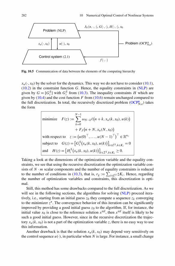
282 10 Numerical Optimal Control of Nonlinear Systems
Fig. 10.5 Communication of data between the elements of the computing hierarchy
xu(·, x0) by the solver for the dynamics. This way we do not have to consider (10.1),(10.2) in the constraint function G. Hence, the equality constraints in (NLP) aregiven by G = [GS
i ] with GSi from (10.3). The inequality constraints H which are
given by (10.4) and the cost function F from (10.6) remain unchanged compared tothe full discretization. In total, the recursively discretized problem (OCPn
N,e) takesthe form
minimize F(z) :=N−1∑
k=0
ωN−k�(n + k, xu(k, x0), u(k)
)
+ FJ
(n + N,xu(N,x0)
)
with respect to z := (u(0)�, . . . , u(N − 1)�
)� ∈ Rnz
subject to G(z) = [GS
i
(xu(k, x0), u(k)
)]i∈E S ,k∈Ki
= 0
and H(z) = [HS
i
(xu(k, x0), u(k)
)]i∈I S ,k∈Ki
≥ 0.
Taking a look at the dimensions of the optimization variable and the equality con-straints, we see that using the recursive discretization the optimization variable con-sists of N · m scalar components and the number of equality constraints is reducedto the number of conditions in (10.3), that is, rg := ∑
i∈E S �Ki . Hence, regardingthe number of optimization variables and constraints, this discretization is opti-mal.
Still, this method has some drawbacks compared to the full discretization. As wewill see in the following sections, the algorithms for solving (NLP) proceed itera-tively, i.e., starting from an initial guess z0 they compute a sequence zk convergingto the minimizer z�. The convergence behavior of this iteration can be significantlyimproved by providing a good initial guess z0 to the algorithm. If, for instance, theinitial value x0 is close to the reference solution xref, then xref itself is likely to besuch a good initial guess. However, since in the recursive discretization the trajec-tory xu(k, x0) is not a part of the optimization variable z, there is no easy way to usethis information.
Another drawback is that the solution xu(k, x0) may depend very sensitively onthe control sequence u(·), in particular when N is large. For instance, a small change

10.1 Discretization of the NMPC Problem 283
in u(0) may lead to large changes in xu(k, x0) for large k and consequently in F(z),G(z) and H(z), which may cause severe problems in the iterative optimization al-gorithm. In the full discretization, the control value u(0) only affects xu(0, x0) andthus those entries in F , G and H corresponding to k = 0, i.e., the functions F(z),G(z) and H(z) depend much less sensitive on the optimization variables.
For these reasons, we now present a third method, which can be seen as a com-promise between the full and the recursive discretization.
Multiple Shooting Discretization
The idea of the so-called multiple shooting discretization as introduced in Bock [4]is derived from the solution of boundary value problems of differential equations,see, e.g., Stoer and Bulirsch [36]. Within these boundary value problems one tries tofind initial values for trajectories which satisfy given terminal conditions. The termshooting has its origins in the similarity of this problem to a cannoneers problem offinding the correct setting for a cannon to hit a target.
The idea of this discretization is to include some components of some state vec-tors xu(k, x0) as independent optimization variables in the problem. These variablesare treated just as in the full discretization except that we do not do this for allk ∈ {0, . . . ,N − 1} but only for some time instants and that we do not necessar-ily include all components of the state vector xu(k, x0) as additional optimizationvariables but only some. These new variables are called the shooting nodes and thecorresponding times will be called the shooting times.
Proceeding this way, we may then provide useful information, e.g., from thereference trajectory xref(·) as described at the end of the discussion of the recursivediscretization for obtaining a good initial guess for the iterative optimization. Muchlike the cannoneer we aim at hitting the reference trajectory, the only difference isthat we do not only want to hit the target at the end of the (finite) horizon but to stayclose to it for the entire time interval which we consider within the optimization.
This motivates to set the state components at the shooting nodes to a value whichmay violate the dynamics of the system (2.1) but is closer to the reference trajectory.This situation is illustrated in Fig. 10.6 and gives a good intuition why the multipleshooting initial guess is preferable from an optimization point of view.
Unfortunately, we have to give up the integrity of the dynamics of the systemto achieve this improvement in the initial guess, i.e., the trajectory pieces startingin the respective shooting nodes can in general not be “glued” together to form acontinuous trajectory. In order to solve this problem, we have to include additionalequality constraints similar to (10.1), (10.2).
For the formal description of this method, we denote the vector of multiple shoot-ing nodes by s := (s1, . . . , srs ) ∈ R
rs where si is the new optimization variable cor-responding to the ith multiple shooting node. The shooting times ς : {1, . . . , rs} →{0, . . . ,N} and indices ι : {1, . . . , rs} → {1, . . . , d} then define the time and the com-ponent of the state vector corresponding to si via

284 10 Numerical Optimal Control of Nonlinear Systems
Fig. 10.6 Resulting trajectories for initial guess u using no multiple shooting nodes (solid), oneshooting node (dashed) and three shooting nodes (gray dashed)
xu
(ς(j), x0
)ι(j)
= sj .
This means that the components xu(k, x0)i , i = 1, . . . , d , of the state vector aredetermined by the iteration
xu(k + 1, x0)i = sj
if there exists j ∈ {1, . . . , rs} with ς(j) = k + 1 and ι(j) = i and
xu(k + 1, x0)i = f(xu(k, x0), u(k)
)i
with initial condition xu(0, x0)i = sj if there exists j ∈ {1, . . . , rs} with ς(j) = 0and ι(j) = i and xu(0, x0)i = (x0)i , otherwise. The shooting nodes si now becomepart of the optimization variable z, which hence reads
z := (u(0)�, . . . , u(N − 1)�, s�)�
. (10.8)
As in the full discretization we have to ensure that the optimal solution of (NLP)leads to values si for which the state vectors xu(k, x0) thus defined form a trajectoryof (2.1). To this end, we define the continuity condition for all shooting nodes sj ,j ∈ {1, . . . , rs} with ς(j) ≥ 1 analogously to (10.1) as
sj − f(xu
(ς(j) − 1, x0
), u
(ς(j) − 1
))ι(j)
= 0, (10.9)
and for all j ∈ {1, . . . , rs} with ς(j) = 0 analogously to (10.2) as
sj − (x0)ι(j) = 0. (10.10)
These so-called shooting constraints are included as equality constraints in (NLP).Since the conditions (10.9) and (10.10) are already in the form of equality con-straints which we require for our problem (NLP), we can achieve this by defining G
to consist of Equalities (10.3), (10.9) and (10.10). As for the recursive discretization,the set of inequality constraints as well as the cost function are still identical to those

10.1 Discretization of the NMPC Problem 285
given by the full discretization. As a result, the multiple shooting discretization ofproblem (OCPn
N,e) is of the form
minimize F(z) :=N−1∑
k=0
ωN−k�(n + k, xu(k, x0), u(k)
)
+ FJ
(n + N,xu(N,x0)
)
with respect to z := (u(0)�, . . . , u(N − 1)�, s�)� ∈ R
nz subject to
G(z) =⎡
⎣[GS
i (xu(k, x0), u(k))]i∈E S ,k∈Ki[sj − f (xu(ς(j) − 1, x0), u(ς(j) − 1))ι(j)]j∈{1,...,rs },ς(j)≥1[sj − (x0)ι(j)]j∈{1,...,rs },ς(j)=0
⎤
⎦ = 0
and H(z) = [HS
i
(xu(k, x0), u(k)
)]i∈I S ,k∈Ki
≥ 0.
Comparing the size of the multiple shooting discretized optimization problem to therecursively discretized one, we see that the dimension of the optimization variableand the number of equality constraints is increased by rs . An appropriate choice ofthis number as well as for the values of the shooting nodes and times is crucial inorder to obtain an improvement of the NMPC closed loop, as the following exampleshows.
Example 10.2 Consider the inverted pendulum on a cart problem from Exam-ple 10.1. For this example, numerical experience shows that the most critical tra-jectory component is the angle of the pendulum x1. In the following, we discuss andillustrate the efficient use and effect of multiple shooting nodes for this variable.
(i) If we define every sampling instant in every dimension of the problem to bea shooting node, then the shooting discretization coincides with the full dis-cretization. Proceeding this way slows down the optimization process signifi-cantly due to the enlarged dimension of the optimization variable. Unless thecomputational burden can be reduced by exploiting the special structure of theshooting nodes in the optimization algorithm, cf. the paragraph on condensingon Sect. 10.4, below, this implies that the number of shooting nodes should bechosen as small as possible. On the other hand, using shooting nodes we maybe able to significantly improve the initial guess of the control. Therefore, interms of the computing time, a balance between improving the initial guess andthe number of multiple shooting nodes must be found.
(ii) If the state trajectories evolve slowly, i.e., in regions where the dynamics isslow, the use of shooting nodes may obstruct the optimization since there maynot exist a trajectory which links two consecutive shooting nodes. In this case,the optimization routine wastes iteration steps trying to adapt the value of theshooting nodes and may be unable to find a solution. Ideally, the shooting nodesare chosen close to the optimal transient trajectory, which is, however, usuallynot known at runtime. Using shooting nodes on the reference, instead, may be agood substitute but only if the initial value is sufficiently close to the reference

286 10 Numerical Optimal Control of Nonlinear Systems
Fig. 10.7 Results for a varying shooting nodes for horizon length N = 14
or if the shooting times are chosen sufficiently large in order to enable thetrajectory to reach a neighborhood of the reference.
(iii) Using inappropriate shooting nodes may not only render the optimization rou-tine slow but may lead to unstable solutions even if the problem without shoot-ing nodes showed stable behavior. On the other hand, choosing good shootingnodes may have a stabilizing effect.
In the following, we illustrate the effects mentioned in (iii) for the horizonsN = 14, 15 and 20. We compute the NMPC closed-loop trajectories for the in-verted pendulum on a cart problem on the interval [0,20] where in each optimiza-tion we use one shooting node for the first state dimension x1 at different timesς(1) ∈ {0, . . . ,N − 1}, and the corresponding initial value to x1 = s1 = −π . In asecond test, we use two shooting nodes for the first state dimension with differ-ent (ς(1), ς(2)) ∈ {0, . . . ,N − 1}2 again with s1 = s2 = −π . Here, the closed-loopcosts in the following figures are computed by numerically evaluating
200∑
k=0
�(xμN
(k, x0),μN
(xμN
(k, x0)))
in order to approximate J∞ from Definition 4.10. Red colors in Figs. 10.7(b),10.8(b) and 10.9(b) indicate higher closed-loop costs.
As we can see from Fig. 10.7(a), the state trajectory is stabilized for N = 14 if weadd a shooting node for the first differential equation. Hence, using a single shootingnode, we are now able to stabilize the problem for a reduced optimization horizonN . Yet, the stabilized equilibrium is not identical for all values ς(1), i.e. for ς(1) ∈{t0, . . . , t2} the equilibrium (π,0,0,0) is chosen, which in our case corresponds tolarger closed-loop costs in comparison to the solutions approaching (−π,0,0,0).Similarly, all solutions converge to an upright equilibrium if we use two shootingnodes. Here, Fig. 10.7(b) shows the corresponding closed-loop costs which allowus to see that for small values of ς(i), i = 1,2, the x1 trajectory converges toward(π,0,0,0).

10.1 Discretization of the NMPC Problem 287
Fig. 10.8 Results for a varying shooting nodes for horizon length N = 15
Fig. 10.9 Results for a varying shooting nodes for horizon length N = 20
As we see, for N = 14 the shooting nodes may change the closed-loop behavior.A similar effect happens for the horizon N = 15. For the case without shootingnodes, the equilibrium (−π,0,0,0) is stabilized, cf. Fig. 10.2. If shooting nodes areconsidered, we obtain the results displayed in Fig. 10.8.
Here, we observe that choosing the shooting time ς(1) ∈ {0,1,3} results in sta-bilizing (π,0,0,0) while for all other cases the x1 trajectory converges toward(−π,0,0,0). Still, for ς(1) ∈ {5, . . . ,9} the solutions differ significantly from thesolution without shooting nodes, which also affects the closed-loop costs. As indi-cated by Fig. 10.8(b), a similar effect can be experienced if more than one shootingnode is used. Hence, by our numerical experience, the effect of stabilizing a chosenequilibrium by adding a shooting node can only be confirmed if ς(1) is set to a timeinstant close to the end of the optimization horizon.
This is further confirmed by Fig. 10.9, which illustrates the results for N = 20.Here, one also sees that adding shooting nodes may lead to instability of the closedloop.
Moreover, we like to stress the fact that adding shooting nodes to a problem maycause the optimization routine to stabilize a different equilibrium than intended.

288 10 Numerical Optimal Control of Nonlinear Systems
Although all equilibria with x1 = (2k +1)π , k ∈ Z, correspond to the same physicalupright position and yield the same value in the running cost, one may expect thatsetting shooting nodes to the value x1 = −π forces the closed-loop trajectory toapproach this particular equilibrium. As we have seen in Figs. 10.7(a), 10.8(a) and10.9(a), this is not always the case since some trajectories approach (π,0,0,0), eventhough this leads to higher closed-loop costs. In particular, Fig. 10.8 shows nicelythat even though the equilibrium (−π,0,0,0) is stabilized without using shootingnodes, fixing a shooting node x1 = −π obstructs the computation of the optimalsolution. Hence, the values of the shooting nodes have to be selected with caresince different choices may result in closed-loop trajectories with different costsand computing times and may have both stabilizing or destabilizing effects.
10.2 Unconstrained Optimization
Now that we have discretized the optimal control problem (OCPnN,e) and trans-
formed it into a nonlinear optimization problem (NLP) in standard form, our aim isto compute a minimizer z, which then gives us an optimal control u for our originalproblem. In this section, we discuss the foundations of all optimization techniques;details for methods like the popular Sequential Quadratic Programming (SQP) orInterior-Point Methods (IPM) are then given in the subsequent section. On the onehand, this allows us to characterize the main principles of such algorithms. On theother hand, it reveals an abstract method, exposes the computationally expensiveparts of such algorithms and allows for rearranging the ordering of these steps toreduce the computational cost.
Although the problem (NLP) is actually a constrained optimization problem, inthis section we present solution methods for dealing with unconstrained optimiza-tion problems since the basic principles, as we will see in Sect. 10.3, are similar tothose in constrained optimization. Since there do not exist any restrictions on theoptimization variable z, the unconstrained optimization problem is a special case ofthe standard (NLP) problem and is given by
minimize F(z)
with respect to z ∈ Rnz .
Due to the sheer size of such a problem, in practice we need to solve it on a computer.The computer, however, cannot deal with this problem in an abstract way, it can onlyevaluate the given functions like the cost function F and possibly its derivative forfinitely many z. Hence, the goal in constructing a solution method for any (NLP)problem is to find a strategy for choosing these evaluation points in order to reliablyidentify a solution of (NLP). While the identification of and the search strategy for asolution are primary goals for a solution method, one still has to keep in mind somesecondary goals like computing time, required memory storage and also the numberof required function evaluations whose detailed analysis is beyond the scope of thischapter but can be found in the standard literature for nonlinear optimization.

10.2 Unconstrained Optimization 289
Focusing on the primary goals, we first need to characterize a solution of a prob-lem (NLP) and how it can be checked whether a given point z ∈ R
nz is a solution.In principle, we are interested in so-called global minimizers.
Definition 10.3 A point z� ∈ Rnz is a global minimizer of the function F : R
nz → R
if F(z�) ≤ F(z) holds for all z ∈ Rnz .
Unfortunately, for general nonlinear—and in particular nonconvex—problemssuch global minimizers are hard to find in practice since we only have local knowl-edge of the function F and its derivative d
dzF . Due to this local knowledge and our
intention to evaluate only a small number of vectors z, we cannot cover the entiredefinition space of F . As a consequence, if we construct an algorithm under theserestrictions we can never be sure if we reached a global minimizer. Nevertheless weare often able to identify a so-called local minimizer.
Definition 10.4 A point z� ∈ Rnz is a local minimizer of the function F : R
nz → R
if there exists a neighborhood N of z� such that F(z�) ≤ F(z) holds for all z ∈ N .
In some cases not all hopes for identifying a global minimizer are lost since wemay have additional information on the function F . For example, if F is convex,then every local minimizer is also a global minimizer. But even if we know that F isconvex, we still need to find such a minimizer. In order not to have to check all valuesz in a certain area, we will assume the function F to be at least twice continuouslydifferentiable, which allows us to use a more practicable way of locating a minimizerusing Taylor’s theorem. Here and in the following we denote derivatives using thefollowing notation, which is common in nonlinear optimization. For a continuouslydifferentiable function g = (g1, . . . , gp) : R
nz → Rp we use the gradient notation
for the Jacobian matrix
∇zg(z) =⎛
⎜⎝
∂g1∂z1
· · · ∂gp
∂z1...
...∂g1∂zn
· · · ∂gp
∂zn
⎞
⎟⎠ ,
which we abbreviate to ∇g if there is no ambiguity. For a twice continuously differ-entiable function g : R
nz → R we write the so-called Hessian as
∇2zzg(z) =
⎛
⎜⎜⎝
∂2g∂z1z1
· · · ∂2g∂z1znz
......
∂2g∂znz z1
· · · ∂2g∂znz znz
⎞
⎟⎟⎠ ,
which we abbreviate to ∇2g if there is no danger of confusion.
Theorem 10.5 Consider a function F : Rnz → R which is continuously differen-
tiable and a direction vector d ∈ Rnz . Then we have
F(z + d) = F(z) + ∇F(z + td)�d (10.11)

290 10 Numerical Optimal Control of Nonlinear Systems
for some t ∈ (0,1). If F is twice continuously differentiable, then we also have
F(z + d) = F(z) + ∇F(z)�d + 1
2d�∇2F(z + td)d (10.12)
for some t ∈ (0,1).
Proof Using the fundamental theorem of calculus, we have
F(z + d) = F(z) +∫ 1
0
d
dtF (z + td) dt.
By the mean value theorem, there exist a t ∈ (0,1) with∫ 1
0
d
dtF (z + td) dt = d
dtF (z + td) = ∇F(z + td)�d,
where we used the chain rule for the second equality. This shows (10.11). By partialintegration we further obtain
∫ 1
0
d
dtF (z + td) dt = d
dt
∣∣∣∣t=0
F(z + dt) +∫ 1
0(1 − t)
d2
dt2 F(z + td) dt
and again using the mean value theorem we get∫ 1
0(1 − t)
d2
dt2 F(z + td) dt = d2
dt2 F(z + t ′d
)∫ 1
0(1 − t) dt = 1
2
d2
dt2 F(z + t ′d
)
for some t ′ ∈ (0, t). Since by the chain rule we have
d
dt
∣∣∣∣t=0
F(z + dt) = ∇F(z)�d and1
2
d2
dt2F(z + t ′d
) = 1
2d�∇2F
(z + t ′d
)d
this shows (10.12). �
The advantage of Taylor’s theorem is that it allows us to introduce knowledge onthe gradient ∇F(z�) and the Hessian ∇2F(z�) into the search for a local minimizerz�. In particular, first-order necessary conditions are derived very easily.
Theorem 10.6 Consider a vector z� ∈ Rnz and a function F : R
nz → R where F
is continuously differentiable in an open neighborhood of z� and z� ∈ Rnz is a local
minimizer of F . Then we have ∇F(z�) = 0.
Proof Suppose ∇F(z�) �= 0 and set d := −∇F(z�). Then we get d�∇F(z�) =−‖∇F(z�)‖2 < 0. Since ∇F is continuous in a neighborhood of z�, there existsa scalar T > 0 such that d�∇F(z� + td) < 0 holds for all t ∈ [0, T ]. By (10.11), forany t ∈ (0, T ] we have F(z� + td) = F(z�) + td�∇F(z� + td) for some t ∈ (0, t).This implies F(z� + td) < F(z�) for all t ∈ (0, T ], which contradicts the local min-imizer property of z�. �
In a similar manner, information on the Hessian can be used to derive second-order necessary conditions from (10.12).

10.2 Unconstrained Optimization 291
Theorem 10.7 Consider a vector z� ∈ Rnz and a function F : R
nz → R where F
is twice continuously differentiable in an open neighborhood of z� and z� ∈ Rnz
is a local minimizer of F . Then we have ∇F(z�) = 0 and the Hessian ∇2F(z�) ispositive semidefinite.
Proof From Theorem 10.6 we know that ∇F(z�) = 0. Now, suppose ∇2F(z�) isnot positive semidefinite and choose a vector d such that d�∇2F(z�)d < 0 holds.Using continuity of ∇2F(z�) in a neighborhood of z�, we know that there exists ascalar T > 0 such that d�∇2F(z� + td)d < 0 holds for all t ∈ [0, T ]. Hence, using(10.12), for any t ∈ (0, T ] and some t ∈ (0, t) we obtain
F(z� + td
) = F(z�)+ t∇F
(z�)�
d + 1
2td�∇2F
(z� + td
)dt < F
(z�).
Similar to the proof of Theorem 10.6, F is strictly decreasing along the direction d ,which contradicts the local minimizer property of z�. �
The results from Theorems 10.6 and 10.7 reveal guidelines to what we are look-ing for, i.e., which properties a local minimizer must fulfill. However, these resultscannot be used to identify a local minimizer once we have found a candidate satisfy-ing the previous conditions. In order to perform such a check, the following theoremcan be used.
Theorem 10.8 Consider a vector z� ∈ Rnz and a function F : R
nz → R where F istwice continuously differentiable in an open neighborhood of z�. If ∇F(z�) = 0 and∇2F(z�) is positive definite, then z� is a local minimizer of F .
Proof Due to F being twice continuously differentiable there exists a radius r > 0such that ∇2F(z) is positive definite for all z ∈ {z | ‖z − z�‖ < r}. Now take anyvector d ∈ R
nz with ‖d‖ < r , then we have z� + d ∈ {z | ‖z − z�‖ < r} and
F(z� + d
) = F(z�)+ d�∇F
(z�)+ 1
2d�∇2F
(z� + td
)d
= F(z�)+ 1
2d�∇2F
(z� + td
)d
for some t ∈ (0,1). Since (z� + td) ∈ {z | ‖z − z�‖ < r}, we have d�∇2F(z� +td)d > 0 and therefore F(z� + d) > F(z�) holds showing the assertion. �
Before we consider constraints we give a short description of the standard strate-gies for nonlinear optimization, the line-search and the trust-region strategy. Bothmethods have in common that they approximately compute local minimizers by it-eratively computing values zk converging to z�. Hence, an initial guess z0 needs tobe supplied by the user for starting the iteration. A good initial guess, i.e., a vectorclose to a minimizer, can usually only be obtained by utilizing knowledge on theprocess. If such knowledge is not at hand, the starting point can be chosen arbi-trarily, however, the convergence speed of the sequence zk toward a minimizer isdrastically reduced in general.
292 10 Numerical Optimal Control of Nonlinear Systems
Within the line-search strategy, the approximation method computes a directiondk in its kth step and searches along the vector dk starting from the current iteratezk for a new iterate zk+1 = zk + αkdk with lower cost function value F(zk+1). Herethe direction dk is typically obtained from minimizing a model function mk whichcatches the local behavior of the cost function F at the current iterate zk and is easyto minimize numerically. Often, quadratic functions of the form
mk(zk + dk) = F(zk) + d�k ∇F(zk) + 1
2d�k Bkdk
are used for this purpose, where Bk is either the Hessian ∇2F(zk) or an approxi-mation of it. The corresponding step length αk > 0 can then, e.g., be determined bysolving the one-dimensional minimization problem
minαk>0
F(zk + αkdk). (10.13)
Once an (approximated) solution to the step length problem has been found, a newsearch direction and a new step length are computed and the scheme is appliediteratively.
In contrast to the line-search approach, the trust-region method takes the onlylocal approximation properties of the model function mk into account when mini-mizing this function in order to determine dk . Since mk can only be guaranteed to bea good approximation close to zk—i.e., it can only be “trusted” in a neighborhood ofzk—the search region for a minimizer of mk is restricted to a so-called trust-region,which is usually given by a ball B�(zk). Hence, the problem consists in computinga suitable next iteration candidate by solving
mindk
mk(zk + dk) where zk + dk ∈ B�(zk). (10.14)
If the candidate zk + dk does not show a sufficient decrease in the cost functionF , then the trust-region is considered to be too large. Hence, the radius � is re-duced and the new minimization problem (10.14) is solved again. Like in the linesearch approach, the model function mk in (10.14) is often generated by quadraticfunctions.
Taking an abstract look on both line-search and trust-region method, the differ-ence between those two approaches lies in the ordering of the basic steps, i.e. findinga search direction and a suitable step length. While the line-search method fixes thesearch direction first and then computes a step length αk , the trust-region methodfirst defines the maximal step length � and then searches for a minimizer using themodel mk .
10.3 Constrained Optimization
So far we have dealt with unconstrained optimization problems and shown the fun-damental results and basic algorithmic ideas which can be used to solve such prob-

10.3 Constrained Optimization 293
lems. In the NMPC algorithm, however, we face the constrained nonlinear optimiza-tion problem
minimize F(z)
with respect to z ∈ Rnz
subject to Gi(z) = 0 for all i ∈ E and Hi(z) ≥ 0 for all i ∈ I(NLP)
in every step of the NMPC iteration where the functions F , G and H are definedby one of the discretizations of the problem (OCPn
N,e) described in Sect. 10.1. Notethat all three discretizations lead to a problem of type (NLP), hence all subsequentresults hold for either of these discretizations.
The index sets in (NLP) are given by E = {1, . . . , rg} and I = {rg + 1, . . . , rg +rh}, respectively, and the functions Gi and Hi are called equality and inequalityconstraints, respectively. These constraints induce the following feasible set, whichwill be important for our upcoming analysis.
Definition 10.9 For a problem (NLP) the set
� = {z∣∣ Gi(z) = 0, i ∈ E ; Hi(z) ≥ 0, i ∈ I
}(10.15)
is called the feasible set and the elements z ∈ � are called feasible points.
Since a minimizer for the problem (NLP) has to be an element of � by definition,we have to modify the definition of a local minimizer in the context of constrainedoptimization problems which we want to approximate later:
Definition 10.10 A point z� ∈ Rnz is a local minimizer of the problem (NLP) if
there exists a neighborhood N of z� such that F(z�) ≤ F(z) holds for all z ∈ N ∩�.
In a similar way as for unconstrained optimization problems, we now want toderive necessary and sufficient conditions which will allow us to construct numeri-cal methods to compute a local minimizer z� of a problem (NLP). As we have seenin the previous Sect. 10.2, the mathematical background of the necessary and suf-ficient conditions given in Theorems 10.6, 10.7 and 10.8 is Taylor’s Theorem 10.5stating results for a linear or quadratic approximation. In constrained optimization,the functions G and H will now also be replaced by suitable approximations. Herewe use linear approximations
G(z + d) ≈ G(z) + ∇G(z)�d and H(z + d) ≈ H(z) + ∇H(z)�d
for this purpose. This, however, only makes sense if the geometry of the feasible set� is—at least locally—reflected properly when G and H are replaced by approxi-mations. To this end so-called constraint qualifications are imposed, which we aregoing to deal with next.
Before we state the popular linear independent constraint qualification (LICQ),we need some definitions. We first introduce the tangent cone T�(z) to the feasibleset �.
294 10 Numerical Optimal Control of Nonlinear Systems
Definition 10.11 A vector v ∈ Rnz is called tangent vector to � at a point z ∈ �
if there exists a sequence of feasible points (zk)k∈N with zk → z, zk ∈ � and asequence of positive scalars (tk)k∈N with tk → 0 such that
limk→∞
zk − z
tk= v (10.16)
holds. The set of all tangent vectors to � at z is called the tangent cone and isdenoted by T�(z).
Note that T� only depends on the geometry of �. The set T�(z) can be seenas a local approximation of all feasible directions at a given feasible point z ∈ �.The feasible directions are all vectors d ∈ R
nz for which z + αd ∈ � holds for allsufficiently small α > 0 and the definition of T� implies that each feasible directionis contained in T�(z). Conversely, for each element v ∈ T�(z) and each ε > 0 thereexists a feasible direction d with ‖d − v‖ < ε.
Obviously, all equality constraints Gi restrict these feasible directions but notnecessarily all inequality constraints: if Hi(z) > 0 holds, then since Hi is contin-uous we get Hi(z + αd) > 0 for all d ∈ R
nz provided α > 0 is sufficiently small.If, however, Hi(z) = 0 holds, then an arbitrarily small change of z in the “wrong”direction may lead to Hi(z + αd) < 0. Hence, all inequality constraints Hi withHi(z) = 0 and all equality constraints Gi may restrict feasible moving directions.These constraints are called active and their indices are characterized by the follow-ing definition.
Definition 10.12 The active set A(z) at any feasible point z consists of the equalityconstraint indices from E together with the indices of the inequality constraints i ∈ Iwhere Hi(z) = 0 holds, that is, A(z) := E ∪ {i ∈ I | Hi(z) = 0}.
Using the active set we can now define a set of “linearized” feasible directionsobtained from the linearizations of H .
Definition 10.13 For a feasible point z ∈ � and the active set A(z) we call the set
F (z) = {v ∈ R
nz∣∣ v�∇Gi(z) = 0 for all i ∈ E and
v�∇Hi(z) ≥ 0 for all i ∈ A(z) ∩ I}
(10.17)
the set (or cone) of linearized feasible directions.
Note that in general we have T�(z) ⊆ F (z), see Fletcher [17, Lemma 9.2.1]. Forthe proof of necessary optimality conditions based on the linearizations of the Gi
and Hi as well as for using the linearized Gi and Hi in our algorithms it is nowimportant to see that these sets coincide. The idea of constraint qualifications is toguarantee that these sets indeed coincide, i.e., that the geometry of T� is capturedby the linearizations of Gi and Hi . Although there is quite a range of differentconstraint qualifications, see, e.g., the book of Mangasarian [26], the linear inde-pendence constraint qualification is probably the most popular one.

10.3 Constrained Optimization 295
Definition 10.14 Consider a feasible point z and the active set A(z). Suppose thatF , G and H are continuously differentiable. If the elements of the gradient set{∇Gi(z) | i ∈ E } ∪ {∇Hi(z) | i ∈ A(z) ∩ I} are linearly independent then we saythat the linear independence constraint qualification (LICQ) holds.
Under this condition we obtain T�(z) = F (z), see Fletcher [17, Lemma 9.2.1].Now we want to proceed as in the unconstrained case, i.e., give characterizations
of minimizers of the cost function F amongst the feasible points z ∈ �. Note that inthe constrained case we cannot simply use Taylor’s Theorem 10.5 to conclude thatif z� ∈ � is a local minimizer for the problem (NLP) then we have ∇F(z�) = 0.
Example 10.15 In order to see that Taylor’s Theorem 10.5 cannot be used in theconstrained case, consider the example of minimizing F(z) = z over � = [−1,1].Obviously z = −1 is a local minimizer, yet we have ∇F(−1) = 1.
The problem with applying Theorem 10.6 in the constrained case is that noboundaries of the constraints sets are included in the analysis in this theorem. Inconstrained optimization, however, we often face the situation of a minimizer lyingon the boundary of the feasible set �, cf. Example 10.15. To deal with this matter,the following auxiliary function L : R
nz × Rrg+rh → R, the so-called Lagrangian
is introduced. For its definition, we combine the constraints Gi and Hi into onefunction C : R
nz → Rrg+rh given by
C : z �→[
(Gi(z))i∈E(Hi(z))i∈I
]
and define a modification of the cost function F by
L(z,λ) := F(z) − λ�C(z). (10.18)
The idea behind this definition is that the additional term −λ�C(z) penalizes viola-tions of the state constraints. The vector λ ∈ R
rg+rh is called Lagrange multiplier.Similar to Theorem 10.6, we can now state a first-order necessary optimal-
ity condition—usually called KKT (Karush–Kuhn–Tucker) condition—in the con-strained case using the Lagrangian (10.18), which will serve as a guideline to findlocal minimizers, see Fletcher [17, Theorem 9.1.1].
Theorem 10.16 Consider the problem (NLP) with local minimizer z� ∈ �. More-over suppose the functions F , G and H to be continuously differentiable and the(LICQ) to hold at z�. Then there exists a Lagrange multiplier λ� ∈ R
rg+rh such thatthe following conditions hold:
∇zL(z�, λ�
) = 0, (10.19)
Gi
(z�) = 0 ∀i ∈ E , (10.20)
Hi
(z�) ≥ 0 ∀i ∈ I, (10.21)
λ�i ≥ 0 ∀i ∈ I, (10.22)
296 10 Numerical Optimal Control of Nonlinear Systems
λ�i Gi
(z�) = 0 ∀i ∈ E , (10.23)
λ�i Hi
(z�) = 0 ∀i ∈ I. (10.24)
The identity (10.24) is a so-called complementarity condition, which says that ei-ther λ�
i = 0 or Hi(z�) = 0 must hold. A special case which is important for nonlinear
optimization algorithms is the following.
Definition 10.17 Consider the problem (NLP) with local minimizer z� ∈ � andLagrange multiplier λ� ∈ R
rg+rh satisfying (10.19)–(10.24). Then we say that thestrict complementarity condition holds if λ�
i > 0 for all i ∈ I ∩ A(z�).
We will use this condition when discussing interior-point methods, below.Interpreting the KKT conditions we see that they connect the gradient of the cost
function to active constraints. In particular, Theorem 10.16 states that for a givenminimizer z� moving along an arbitrary vector v ∈ F (z�) either increases the valueof the first-order approximation of the cost function, i.e. v�∇F(z�) > 0, or keepsits value at the same level in the case v�∇F(z�) = 0.
In the second case—the so-called “critical” case v�∇F(z�) = 0—it is unknownif the cost function value is increasing or decreasing along v. Here second-orderconditions come into play and the curvature information can be used to obtainmore information about change of F along these directions, see Fletcher [17, Theo-rem 9.3.1] for a corresponding proof.
Theorem 10.18 Consider the problem (NLP) with local minimizer z� ∈ �. Supposethe functions F , G and H to be continuously differentiable and the (LICQ) to hold atz�. Let λ∗ ∈ R
rg+rh be a Lagrange multiplier satisfying the KKT conditions (10.19)–(10.24). Then the inequality
v�∇2zzL
(z�, λ�
)v ≥ 0 (10.25)
holds for all
v ∈ C(z�, λ�
) := {v ∈ F
(z�) ∣∣ v�∇Hi
(z�) = 0 for all
i ∈ A(z�) ∩ I with λ�i > 0
}. (10.26)
The set C is also called the critical cone. It contains all directions which leavethe active inequality constraints with λi > 0 as well as all equality constraints activeif one moves a sufficiently small step along these directions. This, however, doesnot need to hold for those active inequality constraints with λi = 0. In particular, wehave the equivalence
v ∈ C(z�, λ�
) ⇐⇒
⎧⎪⎨
⎪⎩
∇Gi(z�)�v = 0, for all i ∈ E ,
∇Hi(z�)�v = 0, for all i ∈ A(z�) ∩ I with λ�
i > 0,
∇Hi(z�)�v ≥ 0, for all i ∈ A(z�) ∩ I with λ�
i = 0.
Now, we want to get a converse result, i.e. we want to check whether a given feasiblepoint is actually a local minimizer. As it turns out, the only differences between the

10.3 Constrained Optimization 297
previous necessary conditions and the sufficient conditions presented next is thatthe constraint qualification is not required whereas Inequality (10.25) needs to bestrengthened to a strict inequality, cf. Fletcher [17, Theorem 9.3.2]:
Theorem 10.19 Consider a feasible point z� ∈ � and suppose a Lagrange multi-plier λ� ∈ R
rg+rh to exist satisfying (10.19)–(10.24). If we have
v�∇2zzL
(z�, λ�
)v > 0 (10.27)
for all v ∈ C(z�, λ�) with v �= 0, then z� is a strict local minimizer of problem (NLP).
We will now focus on the currently common approaches to solve nonlinear con-strained optimization problems (NLP), these are the so-called Sequential QuadraticProgramming (SQP) based on the active set A and the Interior-Point Method (IPM).In the remainder of this section we describe the main ideas of these strategies. Thisdescription cannot replace a thorough treatment as provided, e.g., in the books byBryson and Ho [7], Fletcher [17] or Nocedal and Wright [28], which were also ourmain sources for writing this section. Still, we decided to include this description be-cause we consider it useful for the discussion of certain numerical aspects of NMPCalgorithms in the subsequent Sects. 10.4–10.6.
Active Set SQP Methods
Following the approach outlined at the end of Sect. 10.2, the basic idea of solving(NLP) in the constrained case would be to iteratively determine search directionsdk by solving an auxiliary quadratic optimization problem which approximates F
close to zk , following either the line-search or the trust-region approach. Since wewant to use the necessary conditions from Theorem 10.16, we will also construct asequence λk which is supposed to converge to the Lagrange multiplier λ∗ in Theo-rem 10.16. However, when proceeding this way, the inequality constraints in (NLP)pose a severe problem because they are difficult to handle in a quadratic optimiza-tion problem. There are two ways to overcome this problem. One is to transform theinequality constraints into equality constraints via so-called slack variables; we willuse this method later in the context of interior-point methods. The drawback of thisapproach is that each slack variable is an additional optimization variable and thusthe dimension of the problem may grow significantly.
The alternative which we describe now is the so-called active set method. Herethe fundamental idea is to consider a so-called working set Wk which contains someof the inequality and all equality constraints for the current iteration point zk . Allconstraints within the working set are then treated as equality constraints and theresulting quadratic problem is solved. The working set Wk can be seen as an ap-proximation to the active set A(zk) and is updated in each iteration step. We requirethat the gradients of the constraints contained in the working set are linearly inde-pendent, even if the full set of active constraints at that point has linearly dependentgradients.
298 10 Numerical Optimal Control of Nonlinear Systems
In this setting, the quadratic problem to be solved in each step for determining dk
is obtained from an approximation of the nonlinear problem
minimize F(z)
with respect to z ∈ Rnz
subject to Ci(z) = 0 for all i ∈ Wk
(ECP)
around the current iterate zk . Here Ci denotes the components of the combinedconstraint function C in (10.18) and we assume F and Ci (i.e., G and H ) to be twicecontinuously differentiable. The linear independence requirement for the gradientsof the constraints in the working set implies that the (LICQ) condition holds for(ECP).
Note that we do not intend to solve (ECP) but rather use it for constructing anapproximation in order to determine dk . One way to obtain such an approximationis to apply Newton’s method to the KKT conditions for (ECP). To formulate theseconditions we use the notation λWk in order to denote a Lagrange multiplier inR
rg+rh with λWk
i = 0 for i /∈ Wk . This way we can use the Lagrangian (10.18) fromthe original problem (NLP) for (ECP). With λWk we denote the vector consisting ofthose components of λWk corresponding to indices in Wk , i.e.,
λWk = [(λ
Wk
i
)i∈Wk
].
Denoting the number of elements in Wk by rWk, the vector λWk is an element of
RrWk . Note that λWk is uniquely determined by λWk and vice versa. Furthermore,
we use the notation
CWk (z) = [(Ci(z)
)i∈Wk
]
in order to denote the vector of constraints corresponding to the indices in Wk . Withthis notation, the KKT conditions for (ECP) read
M(z, λWk
) :=(∇zL(z, λWk )
CWk (z)
)= 0. (10.28)
If we apply Newton’s method to this problem, then a step of the resulting iterationis given by
(znew
λWk,new
)=
(z
λWk
)− (∇z,λWk M
(z, λWk
))−1(∇zL(z, λWk )
CWk (z)
)(10.29)
with
∇z,λWk M(z, λWk
) =[∇zzL(z, λWk ) −∇CWk (z)�
∇CWk (z) 0
].
Hence, if sufficient conditions for locally quadratic convergence of the resultingsequence are fulfilled, with this iteration we are able to numerically compute a solu-tion of the problem (ECP). Since we assumed F , G and H to be twice continuouslydifferentiable, we only have to check whether the Jacobian of M(z, λWk ) given in(10.28) is invertible. As we will see in Lemma 10.22, below, invertibility of this

10.3 Constrained Optimization 299
matrix follows at least locally around a minimizer z� of (ECP) from the (LICQ)condition provided z� satisfies the sufficient conditions from Theorem 10.18 for(ECP). Hence, under these conditions quadratic convergence can be guaranteed.
As already mentioned, we do not want to perform the iteration from Newton’smethod in order to solve (ECP). Rather, we would like to apply only one step of thisiteration and then update the working set Wk if needed. While Newton’s method isvery useful for the convergence analysis, cf. Remark 10.23, it turns out that for theactual algorithm it is convenient to replace Newton’s iteration by a different method,which is more closely related to the quadratic approximation idea outlined above.
To this end, let us assume that in the kth iteration of the iterative algorithm forsolving (NLP) we are given iterates zk , λk and a working set Wk . Similar to thedefinition of λWk , above, we define λ
Wk
k to be the vector which coincides with λk
for all components i ∈ Wk and whose components are zero for all i /∈ Wk . We callλ
Wk
k the full multiplier for working set Wk .Now we replace the cost function F in (ECP) by its Lagrangian L. The reason for
using L instead of F will become clear in the discussion after Lemma 10.22, below.Then we approximate the resulting optimization problem by a quadratic programwith linear inequality constraints. This amounts to approximating the Lagrangian L
close to zk by the quadratic function
L(zk + dk, λ
Wk
k
) ≈ L(zk, λ
Wk
k
)+ ∇zL(zk, λ
Wk
k
)�dk + 1
2d�
k ∇2zzL
(zk, λ
Wk
k
)dk
and to replacing the equality constraints Ci(zk + dk) = 0 by their linearizations
Ci(zk + dk) ≈ Ci(zk) + ∇Ci(zk)dk = 0
for all i ∈ Wk . For all dk satisfying these constraints a little computation shows theidentity L(zk, λ
Wk
k ) + ∇L(zk, λWk
k )dk = F(zk) + ∇F(zk)dk , which we can insert
into the approximation of L(zk + dk, λWk
k ). This way, we arrive at the followingquadratic optimization problem:
minimize F(zk) + ∇F(zk)�dk + 1
2d�k ∇2
zzL(zk, λ
Wk
k
)dk
with respect to dk ∈ Rnz
subject to Ci(zk) + ∇Ci(zk)�dk = 0 for all i ∈ Wk .
(EQP)
The Lagrange multiplier for the optimal solution dk of (EQP) according to Theo-rem 10.16 will be denoted by λ
(EQP)k . The key idea of the (SQP) algorithm is to use
these values in order to update zk and λk according to1
zk+1 = zk + dk and λk+1 = λ(EQP)k . (10.30)
Here λ(EQP)k denotes the vector in R
rg+rh whose components (λ(EQP)k )i are defined
by the relations[(
λ(EQP)k
)i, i∈Wk
] = λ(EQP)k and
(λ
(EQP)k
)i= 0 for i /∈ Wk, (10.31)
1Appropriate step lengths αk will be added to these updates, below.

300 10 Numerical Optimal Control of Nonlinear Systems
i.e., we extend the vector λ(EQP)k whose dimension equals the number of indices in
Wk to a vector in Rrg+rh by inserting zeros in the components corresponding to
constraints which are not included in Wk . A motivation for the choice of zk+1 andλk+1 in (10.30) will be given in the discussion after Lemma 10.22, below, and theproblem of determining Wk+1 as well as suitable step lengths αk will be consideredafter we have formulated the basic active set (SQP) algorithm in Algorithm 10.24.
Before we do this, we show how (EQP) can be solved by applying the necessaryand sufficient conditions from Theorems 10.16 and 10.18, respectively, to (EQP).
Lemma 10.20 If λ(EQP)k denotes the Lagrange multiplier corresponding to the op-
timal solution dk of (EQP), then we have
∇2zzL
(zk, λ
Wk
k
)dk + ∇F(zk) = ∇CWk (zk)
�λ(EQP)k . (10.32)
Proof This is an immediate conclusion of Theorem 10.16. �
Combining (10.32) with the constraints in (EQP) we arrive at the following char-acterization of the solution of (EQP).
Lemma 10.21 Given the iterates zk , λk , Wk and the corresponding full multiplierλ
Wk
k for working set Wk , the optimal solution dk of (EQP) and the correspondingLagrange multiplier λ(EQP) fulfill the linear equation system
[∇2zzL(zk, λ
Wk
k ) −∇CWk (zk)�
∇CWk (zk) 0
](dk
λ(EQP)k
)+
( ∇F(zk)
CWk (zk)
)= 0. (10.33)
Proof The stated linear equation system is a combination of the constraints of prob-lem (EQP) and (10.32). �
For the numerical solution it would be more convenient if the matrix in (10.33)was symmetric. Since the Hessian ∇2
zzL(zk, λWk
k ) is symmetric, this can be easilyachieved by multiplying ∇CWk (zk) and CWk (zk) in (10.33) by −1.
The next lemma gives conditions under which (10.33) has a unique solution.
Lemma 10.22 Consider a minimizer z� with Lagrange multiplier λWk,� of (ECP)with working set Wk . Assume that (ECP) satisfies the (LICQ) condition and that z�
satisfies the sufficient conditions from Theorem 10.18 for (ECP). Then there existneighborhoods Nz of z� and Nλ of λWk,� such that there exists a unique solution of(10.33) for all zk ∈ Nz and λ
Wk
k ∈ Nλ.
Proof In order to prove the assertion we show that the matrix
A0 =[∇2
zzL(z�, λWk ,�) −∇CWk (z�)�∇CWk (z�) 0
]
is invertible. This implies the assertion because all expressions in this matrix arecontinuous, hence the invertibility extends to neighborhoods of z� and λWk,�.

10.3 Constrained Optimization 301
In order to prove invertibility of A0 we show
A0
(v
w
)=
(∇2zzL(z�, λWk,�)v − ∇CWk (z�)�w
∇CWk (z�)v
)�= 0,
for all vectors v,w of appropriate dimension with (v�,w�) �= 0. If ∇CWk (z�)v �=0, then we are done. Otherwise, we have ∇CWk (z�)v = 0 and thus either v = 0 orv ∈ C(z�, λWk,�), where C is the critical cone for (ECP). If v = 0, then w �= 0 musthold and since by (LICQ) the matrix ∇CWk (z�) has full column rank we obtain
∇2zzL
(z�, λWk,�
)v − ∇CWk
(z�)�
w = −∇CWk(z�)�
w �= 0.
If v �= 0 then v ∈ C(z�, λWk,�) must hold and by the positive definiteness (10.27) weobtain v�∇2
zzL(z�, λWk,�)v > 0, which implies
v�(∇2zzL
(z�, λWk,�
)v − ∇CWk
(z�)�
w)
= v�∇2zzL
(z�, λWk,�
)v
︸ ︷︷ ︸>0
−v�∇CWk(z�)�
w︸ ︷︷ ︸=w�∇CWk (z�)v=0
> 0,
and thus
∇2zzL
(z�, λWk,�
)v − ∇CWk
(z�)�
w �= 0.
Hence, in all cases we get A0(v�,w�)� �= 0, which shows the desired invertibility
of A0. �
Comparing the system of linear equations (10.33) derived from (EQP) and New-ton’s iteration (10.29) one makes the—at the first glance surprising—observationthat both are identical if in (10.33) we set zk = z, dk = (znew − z), λ
Wk
k = λWk and
λ(EQP)k = λWk,new. However, this identity is not really a coincidence. In fact, the
particular cost function in (EQP) was chosen exactly for the purpose to obtain thisidentity.
Remark 10.23 Interpreting the quadratic problem (EQP) as a Newton iteration isvery useful for the analysis of the convergence speed of the algorithms. Further-more, it provides the motivation for the choice zk+1 = zk + dk and λk+1 = λ
(EQP)k in
(10.30), as these are exactly the values znew and λWk,new from Newton’s iteration.Convergence issues will not be treated in detail here, but we would like to men-
tion that the two properties one would like to have is that the sequences zk , λk con-verge to a KKT point, which follows from Newton’s method provided this methodconverges. Additionally, one would like to ensure that the cost function F decreasesalong the search direction dk if dk �= 0. This decrease property allows to concludethat the limit is a candidate for a local minimizer without having to check second-order conditions.
The formulation of the iteration via (EQP) allows to obtain this decrease propertyunder the conditions of Lemma 10.22 for zk and λ
Wk
k in a neighborhood of z� and
λWk,�k . This is because dk �= 0 implies

302 10 Numerical Optimal Control of Nonlinear Systems
1
2d�
k ∇2zzL
(zk, λ
Wk
k
)dk + ∇F(zk)dk < 0 (10.34)
since otherwise dk = 0 would be the optimal solution. The positive definitenessof ∇2
zzL(z�, λWk,�k ) for directions dk ∈ C(z�, λWk ,�) implies positivity of the first
summand in (10.34) for zk and λWk
k close to these optimal values, hence we obtain∇F(zk)dk < 0. Thus, for α > 0 sufficiently small we get
F(zk + αdk) = F(zk) + ∇F(zk)αdk + O(α2) < F(zk),
i.e., decrease of F along dk . This property is important because it shows that if werestrict the step zk+1 := zk + dk in (10.30) to zk+1 := zk + αkdk then we can stillexpect decrease of the cost function.
There are different ways to couple the solution of (EQP) with the update of theworking set. The approach we explain here relies on the fact that what we actuallywant to solve in each iteration of the algorithms is the following inequality con-strained quadratic program:
minimize F(zk) + ∇F(zk)�dk + 1
2d�k ∇2
zzL(zk, λk)dk
with respect to dk ∈ Rnz
subject to Gi(zk) + ∇zGi(zk)�dk = 0 for all i ∈ E
and Hi(zk) + ∇Hi(zk)�dk ≥ 0 for all i ∈ I .
(IQP)
We will utilize the solution of this program in order to determine the searchdirection dk as well as the new working set Wk+1. Before we explain the details ofthis procedure, we give the basic outline of an active set (SQP) algorithm. In thisbasic version we do not yet include the step length αk , which will be discussed afterAlgorithm 10.25, below.
Algorithm 10.24 (Basic active set (SQP) algorithm) Suppose a pair of initial val-ues (z0, λ0) and an initial working set W0 ⊆ A(z0) to be given and set k := 0.
While convergence test is not satisfied do
1. Compute F(zk), ∇F(zk), ∇2zzL(zk, λk), C(zk) and ∇C(zk)
2. Solve (IQP) using (EQP) and Wk and obtain dk , λ(EQP)k and Wk+1
3. Set zk+1 := zk + dk , λk+1 := λ(EQP)k according to (10.31)
4. Set k := k + 1
As convergence test, here one typically checks whether the necessary conditionsfrom Theorem 10.16 are satisfied up to some user defined tolerance tolOPT.
Furthermore, it should be noted that usually in (SQP) methods one avoids com-puting the Hessian ∇2
zzL(z�, λWk
k ) of the cost function and utilizes computationallycheaper update techniques for obtaining suitable approximations, instead. We willnot discuss this topic here and refer to, e.g., Nocedal and Wright [28] for details.

10.3 Constrained Optimization 303
Now we discuss the details of Step 2 of this algorithm. The solution of (IQP) isobtained by iteratively solving problems of type (EQP) and updating the workingset Wk . This defines another iteration inside the iteration of Algorithm 10.24 whoseiteration index we denote by q . In this inner iteration, we iteratively determine vec-tors d
qk and working sets W q
k , q = 0,1, . . . . We start this iteration with the workingset W 0
k = Wk and initial value d0k , which we assume to be feasible for all constraints
in (IQP). This iteration will terminate after a finite number of steps q� with the opti-
mal value dk = dq�
k of (IQP). The corresponding working set W q�
k will be the activeset of problem (IQP) and will be used as Wk+1 in Algorithm 10.24. The Lagrangemultipliers λ
(EQP)k needed in Algorithm 10.24 are obtained from the last solution of
(EQP) in this iteration. The resulting algorithm will be given in Algorithm 10.25,below. Before we formulate this algorithm, we will now discuss the details of itsdifferent steps.
For its use within this iteration, we rewrite the problem (EQP) in order to takethe previous iterate d
qk into account:
minimize F(zk) + ∇F(zk)�(
pq + dqk
)
+ 1
2
(pq + d
qk
)�∇2zzL
(zk, λ
Wk
k
)(pq + d
qk
)
with respect to pq ∈ Rnz
subject to Ci(zk) + ∇Ci(zk)�(
pq + dqk
) = 0 for all i ∈ W qk .
(EQPq )
Here, for each q we assume that dqk is feasible for the constraints in (IQP)
and for (EQP) with working set Wk = W qk . This implies that the constraints in
(EQPq ) can equivalently be written as ∇Ci(zk)�pq = 0. In order to simplify
the presentation we assume that the problem (EQPq ) is strictly convex, i.e., that(pq)�∇2
zzL(zk, λWk
k )pq > 0 holds for all pq �= 0 with ∇Ci(zk)�pq = 0.
We denote the optimal solution of (EQPq ) by pq,�. From this optimal solutionwe want to construct d
q+1k and a new working set W q+1
k , such that dq+1k is again
feasible for (IQP) and feasible for (EQP) with Wk = W q+1k . To this end, we need to
develop rules for adding and removing constraints from the working set W qk such
that eventually (EQPq ) delivers an optimal solution of (IQP).We first consider the problem of adding constraints, which is closely related to
the definition of dq+1k . Using the previous iterate d
qk and the optimal solution pq,�
of (EQPq ) we define
dq+1k := d
qk + αqpq,� (10.35)
and compute the maximal αq ∈ [0,1] such that dq+1k is feasible for all constraints in
(IQP). Note that if dqk satisfies the constraints contained in the working set W q
k ,
then these constraints are also satisfied for dq+1k for all αq ∈ [0,1]. This is be-
cause Ci(zk) + ∇Ci(zk)�(pq,� + d
qk ) = 0 and Ci(zk) + ∇Ci(zk)
�dqk = 0 imply
∇Ci(zk)�pq,� = 0 and thus

304 10 Numerical Optimal Control of Nonlinear Systems
Ci(zk) + ∇Ci(zk)�(
dqk + αqpq,�
) = Ci(zk) + ∇Ci(zk)�d
qk + αq∇Ci(zk)
�pq,�
= 0.
Hence, for the computation of αq we only need to consider the constraints Hi notcontained in W q
k . If ∇Hi(zk)pq,� ≥ 0 holds for i /∈ W q
k , then we have
Hi(zk) + ∇Hi(zk)� · (dq
k + αqpq,�) ≥ Hi(zk) + ∇Hi(zk)
�dqk ≥ 0
since we assumed dqk to be feasible for (IQP). Hence, αq ≥ 0 can be chosen freely.
In the case ∇Hi(zk)�pq,� < 0, we obtain Hi(zk) + ∇Hi(zk)
� · (dqk + αqpq,�) ≥ 0
only if
αq ≤ −Hi(zk) − ∇Hi(zk)�d
qk
∇Hi(zk)�pq,�
holds true. In order to maximize αq we define
αq := min
{1, min
i /∈W qk ,∇Hi(zk)
�dqk <0
−Hi(zk) − ∇Hi(zk)�d
qk
∇Hi(zk)�pq,�
}. (10.36)
Note that αq = 0 is possible since there might exist an active constraint which isnot an element of the working set W q
k and exhibits ∇Hi(zk)�pq,� < 0. We call
the constraints Hi(zk) for which the minimum is achieved blocking constraints anddenote the set of blocking constraints by
Cq :={j /∈ W q
k
∣∣∣∣ αq = −Hj(zk) − ∇Hj(zk)�d
qk
∇Hj(zk)�pq,�
}. (10.37)
If αq can be chosen to 1, then none of the constraints not contained in W qk is active
for dq+1k and we can set W q+1
k := W qk . If αq < 1, however, then we know that at
least one constraint is active for dq+1k which is not contained in W q
k . Hence, we
construct W q+1k by adding one of the blocking constraints to W q
k .We can iterate this procedure until the resulting algorithm reaches a point d
qk
which minimizes the quadratic objective function in (EQPq ) over its current work-ing set W q
k . This situation can be easily identified since in the optimum we obtainpq,� = 0. Once such a point d
qk is reached, we can decide which of the equality con-
straints in W qk ∩ I should be removed from W q
k because we can only obtain a bettersolution by imposing the inequality constraints Hi(zk) + ∇Hi(zk)(p
q + dqk ) ≥ 0
instead of the equality constraint Hi(zk) + ∇Hi(zk)(pq + d
qk ) = 0. Looking at the
necessary conditions from Theorem 10.16, the constraints corresponding to nega-tive components of the Lagrange multiplier λ
(EQPq )k are natural candidates for this.
However, since a constraint is not checked anymore in the algorithm once the indexi is removed from W q+1
k , we would also like to ensure that it remains satisfied inthe next step, i.e., that it is not immediately reinserted. Fortunately, as we will shownext, the negativity of the respective component of the Lagrange multiplier λ
(EQPq )k
guarantees that this indeed happens.

10.3 Constrained Optimization 305
To this end, consider the iterate dqk yielding pq,� = 0 in (EQPq ) for working
set W qk and the corresponding multiplier λ
(EQPq )k . With (λ
(EQPq )k )ji
we denote thecomponent of the multiplier corresponding to the constraint index i ∈ W q
k and we
assume (λ(EQPq )k )ji
< 0 for some i ∈ W qk ∩ I .
Consider then the solution pq+1,� of (EQPq+1) for working set W q+1k = W q
k \{i}with d
q+1k = d
qk and corresponding multiplier λ
(EQPq+1)k . From Lemma 10.20 we
then obtain
∇2zzL
(zk, λ
Wk
k
)d
qk + ∇F(zk) = ∇CWk (zk)
�λ(EQPq )k
and
∇2zzL
(zk, λ
Wk
k
)(d
qk + pq+1,�
)+ ∇F(zk) = ∇CW q+1k (zk)
�λ(EQPq+1)k .
Subtracting the first from the second equation and using Ci = Hi for i ∈ I we obtain
∇2zzL
(zk, λ
Wk
k
)pq+1,� = ∇CW q+1
k (zk)�(
λ(EQPq+1)k − [(
λ(EQPq )k
)j �=ji
])
− ∇Hi(zk)(λ
(EQPq )k
)ji.
Multiplying from the left with (pq+1,�)� then yields(pq+1,�
)�∇2zzL
(zk, λ
Wk
k
)pq+1,�
= (pq+1,�
)�∇CW q+1k (zk)
�(λ
(EQPq+1)k − [(
λ(EQPq )k
)j �=ji
])
− (pq+1,�
)�∇Hi(zk)(λ
(EQPq )k
)ji.
Since the constraints in (EQPq+1) together with the feasibility of dqk imply the iden-
tity (pq+1,�)�∇CW q+1k (zk) = 0 we thus get
(pq+1,�
)�∇Hi(zk)(λ
(EQPq )k
)ji
= −(pq+1,�
)�∇2zzL
(zk, λ
Wk
k
)pq+1,�.
Hence, the positive definiteness assumption on ∇2zzL(zk, λ
Wk
k ) together with the
inequality (λ(EQPq )k )ji
< 0 yields(pq+1,�
)�∇Hi(zk) > 0.
Consequently, Hi grows along the search direction pq+1,� and may hence be omit-ted in W q+1
k without violating the corresponding inequality constraint in the nextstep.
In practice, not just any index i is chosen but the one corresponding to the mostnegative (λ
(EQPq )k )ji
, which is motivated by sensitivity aspects.Combining all we have derived so far, we end up with the following algorithm
for solving (IQP) to be inserted in Step 2 of Algorithm 10.24.
Algorithm 10.25 (Active set (IQP) algorithm) Suppose a pair of values (zk, λk) aswell as the derivatives ∇F(zk), ∇2
zzL(zk, λk), ∇C(zk), the function values F(zk),C(zk) and a working set Wk ⊆ A(zk) to be given.
306 10 Numerical Optimal Control of Nonlinear Systems
I. Set q := 0, W 0k := Wk and find a starting point d0
k feasible for (IQP) and (EQP)II. While not terminated
a. Solve (EQPq ) to obtain pq,� and λ(EQPq )k
b. If pq,� = 0
• If (λ(EQPq )k )ji
≥ 0 for all i ∈ W qk ∩ I :
terminate with dk = dqk , λ
(EQP)k = λ
(EQPq )k and Wk+1 = W q
k
Else: Set i := argmini∈W qk ∩I (λ
(EQPq )k )ji
, dq+1k = d
qk , W q+1
k := W qk \ {j}
Else
• Compute αq from (10.36) and Cq from (10.37)• Set d
q+1k := d
qk + αqpq,�
• If Cq �= ∅: choose i ∈ Cq and set W q+1k := W q
k ∪ {i}Else: Set W q+1
k := W qk
c. Set k := k + 1
One can show that, apart from certain exceptional cases, this algorithm termi-nates after a finite number of iterations if (IQP) is strictly convex, for details see[28, Sect. 16.4]. Since the solution satisfies the first-order necessary conditions for(IQP), under strict convexity it follows that upon termination the vector dk is theoptimal solution of (IQP). From our construction of the d
qk it additionally follows
that this dk is the optimal solution of (EQP) with working set Wk+1. Methods forfinding the feasible starting point p0
k in Step I are discussed in [28, Sect. 16.4], too.Since dk−1 is feasible for zk−1 and Wk and since zk is typically quite close to zk−1,the vector d0
k = dk−1 is usually a good initial guess.Moreover, this algorithm allows us to maintain the linear independence property
of constraints which are contained in W qk . In particular, if the gradients of the active
constraints of the initial value are linearly dependent, then we can consider a subsetof linear independent constraints. During the iteration we have to add the blockingconstraints. Since the normals of these constraints cannot be represented by a linearcombination of the normals of the constraints contained in the working set W j
k ,linear independence is preserved if one constraint is added. Last, the deletion of aconstraint from the working set W j
k clearly does not lead to linear dependency ofthe remaining constraint normals.
As already mentioned before, in general it is not a good choice to use zk+1 :=zk + dk in Algorithm 10.24. One reason for this is that dk is obtained from mini-mizing a quadratic approximation of F near zk , hence F(zk + dk) may differ con-siderably from the value of this approximation if dk is large. In unconstrained opti-mization, one would hence determine the new zk+1 by solving the one-dimensionalminimization problem (10.13) in the line-search approach or one would restrict dk
by using the trust-region approach (10.14). In both cases, the decrease of the originalnonlinear cost function F is used in order to measure the progress of the algorithm.
In constrained optimization, one also needs to take the constraints into accountwhen measuring this progress. In order to achieve this, one does not use F for

10.3 Constrained Optimization 307
determining zk+1 but rather a function which defines a trade off between decreaseof F and the violation of the constraints, the so-called merit function. In this functionnot only the constraints in the current working set Wk+1 but all constraints in (NLP)are taken into account.
Merit functions are used in both the line-search and trust-region approach, how-ever, the way this function is used is different in both approaches. For trust-regionmethods the merit function determines if the step is accepted or rejected and if thetrust-region radius needs to be adapted. In contrast to that, in the line-search settingthe merit function is used to control the step length itself.
In the following we consider the merit function
L(z,μ) := F(z) + μ∥∥A(z)
∥∥1 (10.38)
with a positive parameter μ > 0 and A(z) defined by
Ai(z) ={
Gi(z), i ∈ E ,
minsi≥0 Hi(z) − si , i ∈ I .
The variables si , i ∈ I are called slack variables and convert the inequality con-straints Hi(z) ≥ 0 into equality constraints minsi≥0 Hi(z) − si = 0. Indeed, using A
the conditions Gi(z) = 0, i ∈ E and Hi(z) ≥ 0, i ∈ I are now compactly expressedas A(z) = 0.
Note that this choice of a merit function is not necessarily the best and differentfunction have been considered in the literature as well, see, e.g., the papers of Han[24], Powell [30] and Schittkowski [33, 34]. For simplicity of exposition, however,we exclusively consider (10.38). The merit function L from (10.38) has the impor-tant property that it decays along the search direction dk from Algorithm 10.24 ifthe working set Wk+1 coincides with the active set of (NLP) and the parameter μ
is sufficiently large, see [28, Lemma 18.2]. This means that as long as there are noactive constraints missing in the current working set, decrease of the merit functionis guaranteed and the algorithm will show progress. Furthermore, one can show thateven though L will in general not be differentiable due to the nonsmoothness of‖A(z)‖1, the directional derivative D(L(z,μ), dk) along the search direction dk inAlgorithm 10.24 does exist.
For the line-search approach, this motivates the following strategy to determinethe new iterate zk+1 = zk + αkdk in Step 3 of Algorithm 10.24: Instead of solving aone-dimensional optimization problem, we use the information from the directionalderivative in order to obtain a computationally less expensive criterion for comput-ing αk using a fixed parameter η ∈ (0,1/2)
3a. Determine μ > 0 such that D(L(z,μ), dk) < 03b. Find αk satisfying L(zk + αkdk,μ) ≤ L(zk,μ) + ηαkD(L(zk,μ);dk)
3c. Set zk+1 := zk + αkdk and update λk+1
Here, the update of λk+1 can be done by using the step width αk in order to defineλk+1 = λk + αk(λ
(EQP)k − λk). Alternatively, cf. [28, Sect. 18.3], one can determine
λk+1 by solving the least squares problem

308 10 Numerical Optimal Control of Nonlinear Systems
minλ
∥∥∇F(zk+1) − CWk+1(zk+1)λ∥∥2
2. (10.39)
The computation of μ in Step 3a. can be done in various ways, e.g., based on aquadratic approximation of L or by using the multiplier λ
(EQP)k .
In the trust-region approach, one solves (IQP) under the additional constraint‖dk‖2 ≤ �k . In the solution method for (IQP) discussed after Algorithm 10.24 thisamounts to including the constraint ‖pq + d
qk ‖2 ≤ �k in (EQPq ). Unfortunately,
due to the additional constraint the problem may arise that the constraints Ci(zk) +∇Ci(zk)
�(pq + dqk ) = 0 cannot be satisfied anymore.
There exists a wide variety of trust-region approaches, for sake of simplicity,however, we now only consider the so-called relaxation approach. In this approach,the original constraints in problem (EQPq ) are modified by a relaxation (or residual)vector rk , that is,
Ci(zk) + ∇Ci(zk)�(
pq + dqk
) = rk,i , (10.40)
where rk can be computed from
rk := C(zk) + ∇C(zk)�ck (10.41)
for ck being the solution of
minimize∥∥C(zk) + ∇C(zk)ck
∥∥22
with respect to ck ∈ Rd subject to ‖ck‖2 ≤ 0.8�k.
(10.42)
The safeguard factor 0.8 guarantees existence of a consistent solution of the relaxedproblem. Since here we work with Euclidean norms, we modify the merit functionto
L(zk,μ) := F(zk) + μ∥∥A(zk)
∥∥2
In order to determine whether the trust-region radius �k should be reduced or not,one compares the decrease of the merit function L with the decrease of a quadraticapproximation Qμ of L. This defines the ratio
ρk := L(zk,μ) − L(zk + dk,μ)
Qμ(0) − Qμ(dk), (10.43)
which is large if the quadratic model Qμ is close to the nonlinear function L andbecomes the smaller the more these functions differ. Since a large difference indi-cates that the values of the nonlinear problem and its quadratic approximation differsignificantly at zk + dk , this will be used as a criterion for reducing the trust-regionradius �k .
Hence, implementing the trust-region idea leads to the following modification ofthe Steps 2 and 3 in Algorithm 10.24, in which we use fixed parameters η ∈ (0,1/2)
and γ ∈ (0,1) and an initial estimate �0 > 0 for the trust-region radius.
2a. Solve problem (10.42) for ck and compute rk from (10.41)2b. Solve (IQP) using the modified constraints (10.40) and ‖dk‖ ≤ �k in (EQPq )
to obtain dk , λ(EQP)k and Wk+1

10.3 Constrained Optimization 309
3a. Determine μ > 0 such that D(L(zk,μ), dk) < 03b. Compute ρk according to (10.43)3c. If ρk > η: Set zk+1 := zk + dk , λk+1 = λ
(EQP)k and choose �k+1 ≥ �k
Else: Set zk+1 := zk and choose �k+1 ≤ γ ‖dk‖Both for the line-search and the trust-region case, the algorithms just given
mainly outline the main idea of these approaches and we refer to the optimizationliterature for all implementational details.
Interior-Point Methods
In contrast to active set methods, the class of interior-point methods generate a se-quence zk which always lies in the interior of the feasible set �. For generatingthis sequence, in each iterate the entire set of inequality constraints H is used. Tothis end, these inequality constraints are transformed into equality constraints usingslack variables, similar to the definition of A in the merit function (10.38). This waythe number of constraints to be considered in each iteration may become consider-ably larger and thus the computational effort in each iteration grows. On the otherhand, one avoids the potentially time consuming identification of the working set.Which of the two advantages is predominant crucially depends on the problem to besolved and can only be assessed on a case by case basis.
Once the constraints are reformulated, the fundamental idea of interior point al-gorithms is to modify the problem under consideration such that all inequality con-straints are always active. In the literature, there are two main ways to achieve thisgoal, the so-called continuation method and the barrier method. These approaches,however, lead to very similar KKT equation systems.
In the continuation (or homotopy) method, the problem
minimize F(z)
with respect to z ∈ Rnz , s ∈ R
ns
subject to Gi(z) = 0 for all i ∈ E ,
Hi(z) − si = 0 for all i ∈ I and si ≥ 0.
(IPM)
is considered where s ∈ Rns are slack variables filling the gap to modify inactive
constraints to be active. The Lagrangian for the problem (IPM) is given by
L(z, s, v,w) = F(z) − v�G(z) − w�(H(z) − s
). (10.44)
Using that at the minimum the equality H(z) = s must hold, for this problem theKKT conditions from Theorem 10.16 can be written as
∇F(z) − ∇G(z)�v − ∇H(z)�w = 0, (10.45)
Sw − μe = 0, (10.46)
G(z) = 0, (10.47)
H(z) − s = 0, (10.48)

310 10 Numerical Optimal Control of Nonlinear Systems
with s ≥ 0, w ≥ 0 and μ = 0, using the vector e := (1,1, . . . ,1)� and the matricesS := diag(s) and W := diag(w) to simplify the notation.
Here the additional parameter μ is introduced as a perturbation parameter inorder to enforce the solution to stay away from the boundary of � by setting μ > 0.More precisely, we consider a sequence of (perturbed) KKT conditions with positiveperturbation parameters μj where μj → 0 as j → ∞. The strict positivity of μj ineach iterate forces the slack variable s and the multiplier w to be positive and thusthe iterates to stay in the interior of �. Similar to the previously mentioned (SQP)methods, the hope is that the limit of the generated sequence satisfies the KKTconditions for problem (IPM) and, if a merit function decreases along the iterates,that the limit is actually a minimizer.
The second, so-called barrier approach consists of a so-called self concordantbarrier function used to encode the feasible set {s ≥ 0} via
minimize F(z) − μ
ns∑
i=1
log si
with respect to z ∈ Rnz , s ∈ R
ns
subject to Gi(z) = 0 for all i ∈ Eand Hi(z) − s = 0 for all i ∈ I
again with parameter μ > 0. In contrast to the homotopy approach where we ex-plicitly stated the constraint s ≥ 0, here it is not necessary to add this constraint tothe barrier approach problem since minimization of the barrier term −μ
∑ns
i=1 log siprevents components of s from becoming too close to zero. As for the continuationmethod, the idea of the barrier approach is to generate approximate solutions for asequence of positive parameters μ which converges to zero.
Applying Theorem 10.16 to the barrier problem, we obtain the conditions
∇F(z) − ∇G(z)�v − ∇H(z)�w = 0, (10.49)
−μS−1e + w = 0, (10.50)
G(z) = 0, (10.51)
H(z) − s = 0, (10.52)
which are identical to (10.45)–(10.48) except for (10.50), which is moreover non-linear in s. However, multiplying (10.50) by S we can easily convert this conditioninto (10.46).
Similar to the (SQP) problem, the ideas of line-search and the trust-region ap-proach can be applied to the (IPM) problem as well. Before discussing these meth-ods, we first look at the application of Newton’s method for solving (IPM). ApplyingNewton’s method to (10.45)–(10.48) we obtain the system of equations
⎛
⎜⎝
∇2zzL(z, s, v,w) 0 −∇G(z)� −∇H(z)�
0 W 0 S
∇G(z) 0 0 0∇H(z) − Id 0 0
⎞
⎟⎠
⎛
⎜⎝
dz
ds
dv
dw
⎞
⎟⎠

10.3 Constrained Optimization 311
= −⎛
⎜⎝
∇F(z) − ∇G(z)�v − ∇H(z)�w
Sw − μe
G(z)
H(z) − s
⎞
⎟⎠ , (10.53)
which is also called primal–dual system (the so-called primal system arises from(10.49)–(10.52) in a similar manner). After computing the step (dz, ds, dv, dw) thenew state iterate can be obtained via
zk+1 = zk + αmaxs dz, sk+1 = sk + αmax
s ds,
vk+1 = vk + αmaxw dv, wk+1 = wk + αmax
w dw,(10.54)
where
αmaxs = max
{α ∈ (0,1] ∣∣ s + αds ≥ (1 − τ)s
},
αmaxw = max
{α ∈ (0,1] ∣∣ w + αdw ≥ (1 − τ)w
} (10.55)
with τ ∈ (0,1), typically 0.995. The latter condition is called fraction to boundaryrule, since it prevents the state and slack variables z and s to reach their lowerbounds too fast. Note that the matrix in (10.53) is regular throughout the iterationfor zk in a neighborhood of an optimal solution which satisfies the second-ordersufficient conditions from Theorem 10.19 and the strict complementarity conditionfrom Definition 10.17. In particular, if the strict complementarity condition holdsat a solution z�, then for every index i we see that either zi or si remains boundedaway from zero as the iterates approach z�, which guarantees that the second blockrow of the matrix in (10.53) has full row rank. Hence, the interior-point approachitself is not ill conditioned and will not show singularities.
In a practical implementation, the matrix in (10.53) is not used. This is due to thefact that transforming the equation system (10.53) into
⎛
⎜⎝
∇2zzL(z, s, v,w) 0 −∇G(z)� −∇H(z)�
0 � 0 Id−∇G(z) 0 0 0−∇H(z) Id 0 0
⎞
⎟⎠
⎛
⎜⎝
dz
ds
dv
dw
⎞
⎟⎠
= −⎛
⎜⎝
∇F(z) − ∇G(z)�v − ∇H(z)�w
w − μS−1e
−G(z)
−H(z) + s
⎞
⎟⎠ (10.56)
for � = S−1W (or � = μS−2 for the primal case), we obtain a symmetric formwhich can be dealt with much more efficiently.
Moreover, the nonconvex case and the fact that the matrix in (10.56) may besingular—if the conditions discussed after (10.55) are not satisfied—have to betreated in order to approximate minimizers instead of mere KKT points and to ren-der the approach applicable, i.e., the matrix to be invertible.
In order to ensure the approximation of a minimizer, as for the (SQP) algorithm(cf. Remark 10.23) we want to ensure that the value of the merit function is decreas-ing during the iteration. To this end, one can show that (dz, ds, dv, dw) is a descentdirection of (10.56) if

312 10 Numerical Optimal Control of Nonlinear Systems
(∇2zzL(z, s, v,w) 0
0 �
)is positive definite on the null space of
(−∇G(z) 0−∇H(z) Id
).
Here, � is positive definite by construction, but ∇2zzL(z, s, v,w) may be indefinite.
To compensate for this deficiency, one can replace the Hessian by ∇2zzL(z, s, v,w)+
δ Id where δ > 0 is sufficiently large to ensure positive definiteness. The size ofthis modification is a priori unknown but can be obtained by successively enlargingδ. Additionally, a possible rank deficiency of ∇G(z) must be considered. In theprimal–dual matrix
⎛
⎜⎝
∇2zzL(z, s, v,w) + δ Id 0 −∇G(z)� −∇H(z)�
0 � 0 Id−∇G(z) 0 γ Id 0−∇H(z) Id 0 0
⎞
⎟⎠
⎛
⎜⎝
dz
ds
dv
dw
⎞
⎟⎠
= −⎛
⎜⎝
∇F(z) − ∇G(z)�v − ∇H(z)�w
w − μS−1e
−G(z)
−H(z) + s
⎞
⎟⎠ (10.57)
this is done by including a regularization parameter γ > 0.Since the iteration (10.54) does not terminate in finite time, we impose the fol-
lowing error function
E(z, s, v,w;μ) = max{∥∥∇F(z) − ∇G(z)�v − ∇H(z)�w
∥∥,
‖Sw − μe‖,∥∥G(z)∥∥,
∥∥H(z) − s∥∥} (10.58)
for some vector norm ‖ · ‖, which will be used for defining a termination criterion.Then, we obtain the following algorithm.
Algorithm 10.26 (Basic interior-point algorithm) Suppose a pair of initial values(z0, s0) to be given and set k := 0.
Compute multipliers v0 and w0, define parameters μ0 > 0, σ, τ ∈ (0,1).While convergence test not satisfied
1. While E(zk, sk, vk,wk;μk) ≥ μk
a. Compute search direction d = (dz, ds, dv, dw) by solving (10.57)b. Determine αmax
s , αmaxw via (10.55)
c. Obtain new iterate (zk+1, sk+1, vk+1,wk+1) from (10.54)d. Set μk+1 := μk and k := k + 1
2. Choose μk ∈ (0, σμk)
Again, for the convergence test it is checked whether the KKT conditions fromTheorem 10.16 are satisfied up to some user defined tolerance tolOPT.
For this algorithm, we can show the following result:
Theorem 10.27 Suppose F , G and H to be continuously differentiable functionsand Algorithm 10.26 to generate a sequence (zk)k=0,...,∞ for a parameter sequenceμk → 0 as k → ∞. Then all points z� with liml→∞ zkj
= z� for some subsequence

10.3 Constrained Optimization 313
kl are feasible. If additionally the (LICQ) condition holds at z�, then the KKT con-ditions from Theorem 10.16 hold at z�.
Proof Let z be the limit point of the sequence zklfrom Algorithm 10.26. Since
μk → 0 holds, the error function (10.58) converges to zero, and we have Gi(zk) → 0and Hi(zk) − sk → 0. Since G and H are continuous, it follows that G(z) = 0,H(z) ≥ 0 and s = H(z) ≥ 0 showing the first assertion.
Since the error function (10.58) converges to zero and si = Hi(z) > 0 for alli /∈ A(z), we obtain [wkl
]i → 0 for all i /∈ A(z). Again using that the error functionconverges to 0 this implies
∇F(zkl) −
∑
i∈E[vkl
]i∇Gi(zkl) −
∑
i∈A(z)
[wkl]i∇Hi(zkl
) → 0. (10.59)
Since by (LICQ) the vectors ∇Gi(z), i ∈ E and ∇Hi(z), i ∈ A(z) are linearly in-dependent and ∇F and ∇H are continuous, the vectors ∇Gi(zkl
) and ∇Hi(zkl) are
linearly independent for all sufficiently large kl , too. It follows that [vkl]i and [wkl
]iin (10.59) are unique and depend continuously on zkl
, hence they converge to some(v, w) ≥ 0. Using continuity of the expressions in the error function, it follows thatthe KKT conditions are satisfied for z with λ = (v�, w�)� as Lagrange multiplier.This proves the second assertion. �
Similar to the Line-Search (SQP) Algorithm, a merit function is imposed in the(IPM) variant of a line-search which may be of the form
L(z, s, ν) = F(z) − μ
ns∑
i=1
log si + ν∥∥G(z)
∥∥ + ν∥∥H(z) − s
∥∥ (10.60)
where the penalty parameter ν needs to be updated throughout the iteration. Notethat we do not have to reprove results concerning descent of the cost function alongthe computed direction since results shown for the (SQP) case carry over to the(IPM) case. The line-search iteration is given by
zk+1 = zk + αsdz, sk+1 = sk + αsds,
vk+1 = vk + αwdv, wk+1 = wk + αwdw,(10.61)
where the step lengths are chosen to satisfy
αs ∈ (0, αmax
s
], αw ∈ (
0, αmaxw
](10.62)
and
L(zk+1, sk+1, ν) ≤ L(zk, sk, ν) + ηαsDL(zk, sk, ν; (dz, ds)
)(10.63)
for some η ∈ (0,1). To incorporate the changes due to the introduction of the meritfunction (10.60), we modify Algorithm 10.26 by defining the fixed parameter η ∈(0,1) and changing Steps 1b to 1d as follows.

314 10 Numerical Optimal Control of Nonlinear Systems
1b. Compute αmaxs , αmax
w via (10.55)1c. Determine αs , αw such that (10.62) and (10.63) hold1d. Obtain new iterate (zk+1, sk+1, vk+1,wk+1) from (10.61)
Similar to the (SQP) method we can also formulate a trust-region version of the(IPM) algorithm in which a trust-region ball constraint ‖(dz, ds)‖2 ≤ �k is addedwith ds = S−1
k ds . This constraint ensures that the quadratic approximation is nottreated as a global model, but only in a small neighborhood of zk . The model prob-lem itself is given by
minimize ∇F(zk)�dz + 1
2d�
z ∇2zzL(zk, s, v,w)dz − μe�ds
+ 1
2d�s Sk�kSkds
with respect to dz ∈ Rnz , ds ∈ R
ns
subject to ∇G(zk)dz + G(zk) = rGk,
∇H(zk)dz − Skds + (H(zk) − sk
) = rHk,
∥∥(dz, ds)∥∥
2 ≤ �k and ds ≥ τe
where the descent direction ds is bounded away from zero by a parameter τ ∈ (0,1).To compute the residuals rGk
, rHka subproblem similar to (10.42) is derived, but
now the variable ck = (cz, cs) is considered:
minimize∥∥∇G(zk)cz + G(zk)
∥∥2
2 + ∥∥∇H(zk)cz − Skcs + (
H(zk) − s)∥∥2
2
with respect to ck ∈ Rnz+ns
subject to ‖ck‖2 ≤ 0.8� and cs ≥ −τ
2e.
(10.64)
Then, the radii rG and rH are given by
rGk= ∇G(zk)cz + G(zk), rHk
= ∇H(zk)cz − Skcs + (H(zk) − sk
). (10.65)
Again similar to the (SQP) case, cf. (10.43), a step is accepted if for the direction(dz, ds) the ratio ρ of the reduction of the merit function L with respect to thepredicted reduction using a quadratic model Qν of the merit function L
ρ = L(z, s, ν) − L(z + dz, s + ds, ν)
Qν(0) − Qν(dz, ds)(10.66)
is at least ρ ≥ η where ν needs to be chosen sufficiently large.To incorporate the trust-region idea into Algorithm 10.26, we introduce the fixed
parameter η ∈ (0,1) and modify Steps (1a) to (1c):
1a. Evaluate normal step ck from (10.64) and radii rG, rH via (10.65)1b. Compute solution dz, ds for quadratic model of (IPM) and retrieve ds = Sds
1c. Obtain ρ from (10.66)If ρ ≥ η: Set zk+1 = zk + dz, sk+1 = sk + ds , update multipliers vk , wk andchoose �k+1 ≥ �k
Else: Set zk+1 = zk , sk+1 = sk , vk+1 = vk , wk+1 = wk and choose �k+1 < �k

10.4 Implementation Issues in NMPC 315
Fig. 10.10 Architecture of NMPC solver
Here, the update of the Lagrange multipliers can be done similar to the leastsquares approach outlined in (10.39).
Note that there also exist other types of solvers for the general (NLP) problemlike penalty and augmented Lagrangian methods, which we do not discuss here.Additionally, there exists a wide variety of solvers for quadratic problems which wedid not mention here but which are of particular interest: on the one hand, quadraticproblem solvers are required within (SQP) and (IPM) algorithms. On the other hand,many practical problems directly lead to a quadratic cost function.
Additionally, many extensions, modifications and improvements for the pre-sented algorithms have been developed whose explanation is beyond the scope ofthis section; some of these are given in a short overview in Sect. 10.7.
10.4 Implementation Issues in NMPC
So far, we discussed the numerical components which are typically part of an NMPCalgorithm and whose interplay is sketched in Fig. 10.10. Our aim now is to combinethese components, i.e., the differential equation solver from Chap. 9, the discretiza-tion technique from Sect. 10.1 and the optimizer from Sect. 10.3, and to analyze theinteractions and effects between them.
Since the interaction heavily depends on the used implementation, one cannotgive a complete analysis. Therefore, the aim of this section is to give some guide-lines regarding the interplay of the components with respect to certain key param-eters such as the tolerance values for the optimization and integration, the horizonlength or the number of multiple shooting nodes.

316 10 Numerical Optimal Control of Nonlinear Systems
Structure of the Derivatives
We start by analyzing the connection between the discretization and the optimiza-tion method. As we have seen in Sect. 10.3, both the (SQP) and the (IPM) algorithmsrequire derivatives of the cost function and the Jacobian of the constraints in order tocompute a search direction dk . Since for many examples algebraic expressions forthese function are not at hand, these derivatives need to be computed numerically.To this end, in the continuous time case one may numerically solve the variationalequation (cf. Hairer and Wanner [23, Sect. I.14]). Alternatively, one may directlyapproximate all derivatives by difference quotients with respect to every componentof the optimization variable z. Here we follow this second approach, which approx-imates the directional derivative of a function g : R
nz → Rp at a point z in direction
v via
∇g(z)�v = limt→0
g(z + t · v) − g(z)
t≈ g(z + t · v) − g(z)
t(10.67)
for small t > 0. Here, the step length t should be chosen depending on the usedcomputer, i.e. its floating point accuracy. Using the ith unit vector v = ei , we thusobtain an approximation of the ith row of the Jacobi matrix ∇g(z).
Note that if g involves the solution of a continuous time optimal control problemusing the methods from Chap. 9, then the computation of the difference quotient(10.67) may depend sensitively on the time grids used to compute g(z + t · v) andg(z). To circumvent this problem, a synchronized evaluation of f for the nominalvector z and for the disturbed vectors z + t · v using the same grid for both compu-tations can be used.
A similar problem arises from a possible integral type cost function (3.4), whichhas to be evaluated along the trajectory. To this end, we use the technique describedin Sect. 9.4, i.e., we include the integral as an additional component in the ordi-nary differential equation and use the same discretization for the evaluation of thisintegral and the dynamics of the problem, see also the paper of Gyurkovics andElaiw [22] for a detailed analysis in an NMPC context.
Most if not all common optimization algorithms use an approximation B(z) ofthe Hessian ∇zzL of the cost function which can be obtained, e.g., by so-calledDFP (Davidon–Fletcher–Powell) [10, 18] or BFGS (Broydon–Fletcher–Goldfarb–Shanno) updates [6, 16, 19, 35]. For this reason, the computationally most expensivepart within each step of the optimization algorithm is the evaluation of the Jacobian∇C(z) of the constraints. We now consider this problem in some more depth forthe shooting discretization. In the following, r = rg + rh denotes the number ofconstraints and—as before—rs the number of shooting nodes. Using that the op-timization variable z ∈ R
nz is of the form z = (u(0)�, . . . , u(N − 1)�, s�)�, thisJacobi matrix has the structure sketched in Fig. 10.11.
This figure indicates that the number of function evaluations is growing quadrat-ically in the horizon length N , which is therefore the dominating parameter for thecomputing time of the optimization algorithm. For this reason, setting up an NMPCscheme which is stable for small optimization horizon N—for instance by choos-ing a good cost function in the sense of Sect. 6.6, by adding terminal weights as

10.4 Implementation Issues in NMPC 317
Fig. 10.11 Structure of the Jacobian of the constraints ∇zC(z)�
described in Sect. 7.2 or by using the adaptation techniques of Sect. 7.8—will ingeneral significantly reduce the computational effort.
Regardless of the length of the horizon, a recomputation of the Jacobian ∇C(z)
has to be performed for a large number of the iteration steps within any of the pre-sented minimization routines. Hence, an efficient implementation to evaluate thismatrix is required. Additionally, efficient (SQP) and (IPM) implementations usuallyupdate only a few entries of the Jacobian whereas for the other entries the lineariza-tion is considered to be sufficiently accurate. This implies that an efficient imple-mentation of the evaluation of the Jacobian should perform only those evaluationsof the dynamics of the system needed for the entries of the Jacobian which are ac-tually requested by the optimization algorithm.
We now sketch such an efficient evaluation which is based on the following ob-servation: if we look at the way the predicted states xu(k, x0) depend on the controlvalues u(n), one observes the triangular structure sketched in Fig. 10.12, in whichthe arrows indicate increasing indices k and n.
This structure is due to that fact that changing u(n) does not affect the statetrajectory values xu(k, x0) for k ∈ {0, . . . , n}.
Our proposed efficient implementation builds upon this observation. Assume thatthe columns of ∇C(z)� colored in dark gray in Fig. 10.13 have to be recomputed.To this end, we need to evaluate the nominal function C(z) as well as the perturbed

318 10 Numerical Optimal Control of Nonlinear Systems
Fig. 10.12 Dependence ofxu(k, x0) on u(n)
values C(z + tei) for those i corresponding to the dark gray columns. Each of theseevaluations requires the computation of a trajectory following the rules describedbefore (10.8). Since z = (u(0)�, . . . , u(N − 1)�, s�)�, each ei either correspondsto an entry of a control vector u(n) or to a shooting node sk . Let us first considerthose ei which correspond to entries of control vectors and denote the time index ofthe corresponding control vectors by ni . Then the definition of z yields that i1 ≥ i2implies ni1 ≥ ni2 .
The structure from Fig. 10.12 now implies that the nominal trajectory xu cor-responding to z and the perturbed trajectory xu′ corresponding to z + tei satisfyxu(k) = xu′(k) for k = 0, . . . , ni . This means that these values can be reused forxu′ and do not need to be recomputed. Hence, for each perturbed trajectory to becomputed one could copy the nominal trajectory and then change only those entrieswhich do not coincide. While this approach is already very efficient in terms of thenumber of function evaluations, it is not efficient in terms of memory access be-cause we need to make many copies of the nominal trajectory. Since memory accessis one of the bottle necks in modern computers, this procedure will be quite timeconsuming.
To solve this problem we use a second implication of Fig. 10.12: consider twoperturbed trajectories xu1 and xu2 corresponding to z+ tei1 and z+ tei2 with i1 ≥ i2.Then the time indices of the corresponding control vectors satisfy ni1 ≥ ni2 andconsequently the triangular structure from Fig. 10.12 yields the identity xu1(k) =xu2(k) holds for k = 0, . . . , ni . This means that when computing xu2(k), insteadof using the values of the nominal trajectory xu we may also use the values ofany perturbed trajectory xu1 with i1 ≥ i2. Thus, if we schedule the computations ofC(z + tei) such that the indices i are monotone decreasing, then we can compute

10.4 Implementation Issues in NMPC 319
Fig. 10.13 Efficient implementation for computing the Jacobian ∇zC(z)�
each perturbed trajectory by modifying the perturbed trajectory computed before,i.e., we can compute all entries in the Jacobian by working on a single copy of thenominal trajectory instead of having to make many copies.
The indices ei corresponding to shooting nodes can be treated in the same mannerobserving that again the change of a shooting node only affects the solution at timesgreater or equal than the shooting time.
The resulting scheduling of the computations is indicated by the arrows inFig. 10.13. The two thicker arrows pointing to the right correspond to the computa-tion of the nominal trajectory for the control and the shooting values, respectively,and the thinner arrows pointing to the left indicate the order of the computations ofthe perturbed trajectories w.r.t. the indices of the corresponding ei .
An alternative to this efficient sequential scheduling is given by parallelizationof the computations of the perturbed trajectories. Except for the evaluation of thenominal trajectory, all evaluations of the dynamics (2.1) (or (2.8) in the continuoustime case) required to compute ∇C(z) and ∇F(z) are fully decoupled and may beexecuted in parallel. Hence, if the problem is large and many cores can be used toparallelize these computations, a significant speedup can be expected.

320 10 Numerical Optimal Control of Nonlinear Systems
Condensing
As outlined in the discussion of Fig. 10.11, the computation of the Jacobian of theconstraints massively depends on the number of optimization variables of the dis-cretized optimal control problem. Hence, according to Sect. 10.1 the minimal num-ber of optimization variables is N · m for control values u ∈ R
m. Adding multipleshooting nodes increases the number of optimization variables but may also improvethe numerical solutions, cf. Example 10.2. In the following, we present an approachwhich allows us to reduce the additional numerical effort induced by using shootingnodes and which has become quite popular in the NMPC community, the so-calledcondensing of constraints, see, e.g., Diehl [11] or the paper by Bock and Plitt [5].
In order to simplify the exposition, here we apply the method to the full dis-cretization technique, which can be regarded as a special case of the multiple shoot-ing technique in which each component of the solution vector at each samplinginstant is a shooting node. To simplify notation, we now define sj to be a vector ofdimension d , which allows us to get rid of the index function ι(·), and we set the in-dex function ς(·) to be the identity function. According to this change, the equalityconstraints induced by the continuity conditions (10.1) take the form
S(z) := [[sj+1 − f
(sj , u(j)
)]j∈{0,...,N−1}
] = 0.
Using a Newton like approach for the KKT conditions from Theorem 10.16, asoutlined for the active set and interior-point methods in Sect. 10.3, we obtain thelinearized continuity condition
S(z) + ∇zS(z)��s = 0 (10.68)
where �s denotes the part of the search direction d corresponding to the shootingnodes. Within this equation, the Jacobian of S(z) takes the sparse form
∇zS(z)� =
⎛
⎜⎜⎜⎜⎝
− ∂f (s0,u(0))∂s0
1 0 · · · · · · 0
0 − ∂f (s1,u(1))∂s1
1 0 · · · ...
.... . .
. . .. . . 1 0
0 · · · · · · 0 − ∂f (sN−1,u(N−1))
∂sN−11
⎞
⎟⎟⎟⎟⎠
.
This allows us to compute �s from (10.68) via
⎛
⎝�s1
...
�sN
⎞
⎠ =
⎛
⎜⎜⎜⎜⎝
∂f (s0,u(0))∂s0
0 · · · 0
0 ∂f (s1,u(1))∂s1
0...
.... . .
. . . 00 · · · 0 ∂f (sN−1,u(N−1))
∂sN−1
⎞
⎟⎟⎟⎟⎠
⎛
⎝�s0
...
�sN−1
⎞
⎠− S(z),
i.e., �s1, . . . ,�sN can be computed from �s0, which is in the search direction forthe shooting node corresponding to the initial value. Hence, if we solve (10.68)outside the discretized optimal control problem, then the fully discretized problemreduces to a shooting discretization in which only the components of the initial
10.4 Implementation Issues in NMPC 321
value are considered to be shooting nodes, i.e. rs = d . Note that the dynamics ofthe system still have to be evaluated using the initial values given by the shootingnodes of the original problem. However, apart from this technical difference, thecondensing technique allows us to use a full multiple shooting discretization of theoptimal control problem while the complexity of the problem handed over to theoptimization algorithm is reduced to a multiple shooting discretization with only d
instead of d · (N + 1) shooting nodes.A useful side effect of using the full discretization we would like to mention is
that all evaluations of the dynamics (2.1) (or (2.8) in the continuous time case) arefully decoupled. Hence, computing all components of the (discretized) optimiza-tion problem can be done in parallel, which may lead to a significant speedup ingenerating the iterates of the optimization problem.
Optimality and Computing Tolerances
Let us now turn to the investigation of the interplay of the different numerical accu-racies in the optimization method and the differential equation solver. In particular,we analyze the impact of the user dependent choices of tolerance values for thesetwo components on the stability of the closed-loop system on the one hand, and onthe resulting computing time on the other hand. For the differential equations solver,the tolerance tolODE is the parameter discussed in Sect. 9.3. For the optimizationroutine, the parameter tolOPT is the accuracy up to which the sufficient KKT con-ditions of Theorem 10.16 are satisfied. Both tolOPT and tolODE are assumed to besmall in this section. The situation in which the optimization is terminated beforethe necessary conditions are approximately satisfied, which was theoretically inves-tigated in Sect. 7.9, will be discussed in Sect. 10.6.
To illustrate effects of different choices for the tolerance levels, let us first givethe following example.
Example 10.28 Consider the inverted pendulum Example 10.1. As tolerances forthe differential equation solver and the optimization algorithm we consider the gridof parameters
(tolOPT, tolODE) ∈ {10−8,10−7, . . . ,10−1}2
in order to evaluate the NMPC controller μN . The resulting closed-loop trajectoryxμN
(·, x0) was computed on the interval [0,20] with sampling period T = 0.1, ini-tial value x0 = (2,2,0,0) and numerical accuracy tolODE = 10−10. By using a muchsmaller tolerance for computing xμN
(·, x0) we “emulate” the setting of Sect. 9.5 inwhich the computation of μN is affected by numerical errors and the closed-loopsolution is obtained by using the numerically computed μN and the exact dynamics.
Let us first consider one of the critical cases mentioned in Example 10.1 and setthe horizon length to N = 53. In this case, the numerical results in Figs. 10.14 il-lustrate that the parameters (tolOPT, tolODE) should be chosen carefully due to their

322 10 Numerical Optimal Control of Nonlinear Systems
Fig. 10.14 Exceptional closed-loop costs for N = 53 and various optimization and differentialequation solver tolerances
effects on the closed loop. The closed-loop costs in the following figures are com-puted as in Example 10.2.
Here, Fig. 10.14(a) shows that for some pairs (tolOPT, tolODE) the closed-loopcosts are significantly higher. If we analyze the corresponding closed-loop trajecto-ries, these costs correspond to solutions which are driven to the downward position(−2π,0,0,0) for tolOPT = 10−1 and several values considered for tolODE, cf. thedotted lines in Fig. 10.14(b). All other pairs, however, do “mainly” cause the pen-dulum to tend toward an upright position. However, these positions vary in twoways. For one, the x1-component of the closed-loop trajectory does not convergeto the same upright position, similar to what we observed in Example 10.2. And,more importantly, once an upright position is reached, the trajectory may becomeunstable and move to another upright position, an effect we already observed in Ex-ample 10.1. In this case, the observed closed-loop costs increase due to the repeatedtransitions between different upright positions, see again Fig. 10.14(a).
The reasons for this unpredictable behavior can be found in the implementationand the unstable nature of the equilibrium which we want to stabilize. One source oferrors is the tolerance tolODE used in computing μN . Since the closed-loop trajec-tory is always computed with accuracy tolODE = 10−10 and the open-loop predic-tions are computed with different tolerance levels of the differential equation solver,the solutions deviate slightly. Consequently, according to Theorem 9.10, we canonly expect practical asymptotic stability and the radius δ of the neighborhood towhich the solutions converge according to Definition 9.9 will grow with the toler-ance tolODE used in the computation of μN (and most likely also with tolOPT, eventhough this was not rigorously analyzed in Sect. 9.5). Once δ becomes too large,the pendulum may leave a neighborhood of the upright equilibrium and move toanother upright position.
Another source of errors stems from the fact that the optimization algorithm doesnot yield a globally optimal solution. In fact, since the problem is nonconvex we canin general never guarantee to obtain a globally optimal solution, but the growth of
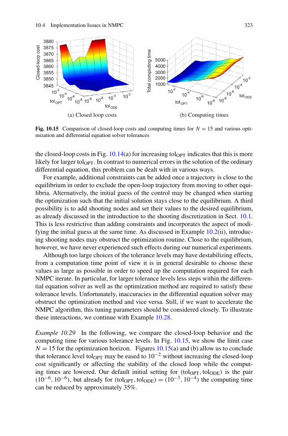
10.4 Implementation Issues in NMPC 323
Fig. 10.15 Comparison of closed-loop costs and computing times for N = 15 and various opti-mization and differential equation solver tolerances
the closed-loop costs in Fig. 10.14(a) for increasing tolOPT indicates that this is morelikely for larger tolOPT. In contrast to numerical errors in the solution of the ordinarydifferential equation, this problem can be dealt with in various ways.
For example, additional constraints can be added once a trajectory is close to theequilibrium in order to exclude the open-loop trajectory from moving to other equi-libria. Alternatively, the initial guess of the control may be changed when startingthe optimization such that the initial solution stays close to the equilibrium. A thirdpossibility is to add shooting nodes and set their values to the desired equilibrium,as already discussed in the introduction to the shooting discretization in Sect. 10.1.This is less restrictive than adding constraints and incorporates the aspect of modi-fying the initial guess at the same time. As discussed in Example 10.2(ii), introduc-ing shooting nodes may obstruct the optimization routine. Close to the equilibrium,however, we have never experienced such effects during our numerical experiments.
Although too large choices of the tolerance levels may have destabilizing effects,from a computation time point of view it is in general desirable to choose thesevalues as large as possible in order to speed up the computation required for eachNMPC iterate. In particular, for larger tolerance levels less steps within the differen-tial equation solver as well as the optimization method are required to satisfy thesetolerance levels. Unfortunately, inaccuracies in the differential equation solver mayobstruct the optimization method and vice versa. Still, if we want to accelerate theNMPC algorithm, this tuning parameters should be considered closely. To illustratethese interactions, we continue with Example 10.28.
Example 10.29 In the following, we compare the closed-loop behavior and thecomputing time for various tolerance levels. In Fig. 10.15, we show the limit caseN = 15 for the optimization horizon. Figures 10.15(a) and (b) allow us to concludethat tolerance level tolOPT may be eased to 10−2 without increasing the closed-loopcost significantly or affecting the stability of the closed loop while the comput-ing times are lowered. Our default initial setting for (tolOPT, tolODE) is the pair(10−6,10−6), but already for (tolOPT, tolODE) = (10−3,10−4) the computing timecan be reduced by approximately 35%.

324 10 Numerical Optimal Control of Nonlinear Systems
There are several guidelines which can be drawn from this example, and whichhave shown to be reasonable in our numerical experiments.
First, the horizon length should always be chosen to be as small as possible be-fore different tolerance levels are considered. The reasons for this are twofold: Forone, the additional complexity of an enlarged horizon always leads to an increasein the computing time to solve the optimal control problem. While this may becompensated by increasing the tolerance levels of the optimizer and the differentialequation solver, another aspect comes into play, which we have not yet discussed:increasing the tolerance level of the differential equation solver may heavily corruptthe numerical evaluation of the derivatives needed in the optimization algorithm.For this reason, the optimization iteration may be unable to converge toward a pointsatisfying the KKT conditions of Theorem 10.16 with accuracy less than tolOPT.
As a consequence, the tolerance levels should always satisfy tolOPT � tolODE.Here, we use this imprecise formulation on purpose since properties of the differen-tial equation like its rate of change or simply its scale influence the “best” relationbetween these two tolerance parameters. Yet, it is usually reasonable to set the tol-erance level of the differential equation solver to be smaller than the tolerance levelof the optimization method.
10.5 Warm Start of the NMPC Optimization
In the previous section, we concentrated on solving Step (2) of Algorithm 3.11,which is computationally quite demanding. Although it is not obvious from thealgorithm itself, the consecutive Step (3) can be used to significantly reduce thetime required to solve the subsequent problem of type (OCPn
N,e). More precisely,the optimal solution u� of (OCPn
N,e) at time n can be efficiently used in order toconstruct an initial guess for (OCPn
N,e) at time n+ 1. In order to see how this can bedone, one needs to take a closer look to the time evolution of the NMPC problemitself as displayed in Figs. 10.16 and 10.17 for a sampled data continuous timesystem with sampling period T . For better visibility, in these figures we have plottedthe whole continuous time trajectory instead of only the discrete values of xu(·, x0).
Figure 10.16 schematically sketches the step of solving the problem (OCPnN,e) for
a given initial value x0 for the nth iterate of the NMPC procedure. As a result, a pre-diction of the trajectory xu(·, x0) on the considered time horizon and a minimizingcontrol sequence u�(·) ∈ U
N(x0) are obtained.Now, according to Step (3) of Algorithm 3.11, the first element of the control
sequence u�(·) is used as control value in the next sampling period, see Fig. 10.17for a schematical sketch. However, the algorithm does not say what should be donewith the remainder of the control sequence. The most simple approach is to simplydiscard these values and go to the next iterate. Yet, as obvious from Fig. 10.17, thesequence contains a lot of information on the prediction at time n + 1.
Hence, this information should be reused in the subsequent (n+1)st NMPC step.In particular, one has to keep in mind that in most cases an iterative solver is usedto compute the optimal control u�(·) for problem (OCPn
N,e). As mentioned in the

10.5 Warm Start of the NMPC Optimization 325
Fig. 10.16 Step (2) of Algorithm 3.11
Fig. 10.17 Step (3) of Algorithm 3.11
previous Sect. 10.3, one can only guarantee local convergence for such solvers, i.e.,a good initial guess is required. Furthermore, supplying a good initial guess willreduce the number of iterations to be performed by both the (IPM) and the (SQP)method.
In what follows we will explain three methods to address the “good initial guess”problem.
Initial Value Embedding
The initial value embedding technique proposed by Diehl, Bock, Schlöder, Find-eisen, Nagy and Allgöwer [12] is used for fully discretized problems (OCPN,e)
326 10 Numerical Optimal Control of Nonlinear Systems
which are solved using (SQP) methods. The approach utilizes the fact that the sub-sequent problem differs only in the initial value x0. In particular, taking a closerlook at the problem (NLP) using full discretization, one can see that the problemdepends linearly on the x0 in the equality constraint
xu(0, x0) − x0 = 0 (10.69)
where xu(0, x0) is the first entry of the optimization vector z as displayed in (10.5).Now, if the (SQP) solver handling the subsequent problem (OCPN,e) with time indexn + 1 is initialized via
z0 := z� = (xu�(0, x0)
�, . . . , xu�(N,x0)�, u�(0)�, . . . , u�(N − 1)�
)�
where z� is the optimal solution of the nth problem (OCPN,e), then most of the dataof the previous linear problem
[∇2zzL(z�, λWk,�) −∇CWk (z�)�∇CWk (z�) 0
](d�
λ(EQP),�
)+
( ∇F(z�)
CWk (z�)
)= 0 (10.70)
solved at time n, cf. Algorithm 10.25, can be reused for the first (SQP) step at timen + 1. This is because only those very few entries in (10.70) which depend on thenew initial value xnew
0 at time n + 1 need to be updated. Hence, the approximationin the first (SQP) step at time n + 1 is almost readily computed. Note, however,that this advantage only holds for the full discretization, since for the recursivelydiscretized problem all values in (10.70) depend on x0 and thus all gradients needto be recomputed. Furthermore, this procedure becomes less efficient in the case ofnonconstant reference xref because in this case � and thus F change with time andthe respective gradients have to be recomputed, too.
If, moreover, x0 and xnew0 differ only slightly, as it is the case for small sampling
periods, then the remaining entries in (10.70) may still be sufficiently accurate inorder to allow for an accurate solution of (OCPN,e) for the new initial value xnew
0 .In this case, a single (SQP) iteration is sufficient in order to deliver a sufficientlyaccurate solution at time n+ 1. Furthermore, since the constraint (10.69) is linear inx0 = xnew
0 , the infeasibility introduced by inserting xnew0 will be removed after this
single iteration.An interesting application of the initial value embedding technique is the so-
called real-time iteration, cf. the articles of Ferreau, Bock and Diehl [14] and Best[3]. In this approach one updates the control sequence several times in one samplinginterval, assuming, of course, that the used hardware (sensors, actuators etc.) allowsfor a faster sampling of the control variable u. The structure of the resulting schemedoes not fully comply with the theoretical analysis in the previous chapters, butwe conjecture that it can be analyzed by suitably extending the multirate samplingapproach discussed before Remark 2.9.
In the real-time iteration, one exploits the linear dependence of the fully dis-cretized problems on x0 and uses parametric active set methods. To this end, a scalar
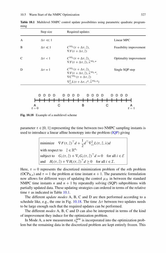
10.5 Warm Start of the NMPC Optimization 327
Table 10.1 Multilevel NMPC control update possibilities using parametric quadratic program-ming
Step size Required updates
A �τ ≪ 1 Linear MPC
B �τ � 1 CWk (τ + �τ, z),∇F(τ + �τ, z)
Feasibility improvement
C �τ < 1 CWk (τ + �τ, z),∇F(τ + �τ, z), λWk ,�
Optimality improvement
D �τ = 1 CWk (τ + �τ, z),∇F(τ + �τ, z), λWk ,�,∇CWk (τ + �τ, z)
Single SQP step
∇2zzL(τ +�τ, z�, λWk ,�)
Fig. 10.18 Example of a multilevel scheme
parameter τ ∈ [0,1] representing the time between two NMPC sampling instants isused to introduce a linear affine homotopy into the problem (IQP) giving
minimize ∇F(τ, z)�d + 1
2d�∇2
zzL(τ, z, λ)d
with respect to z ∈ Rnz
subject to Gi(τ, z) + ∇zGi(τ, z)�d = 0 for all i ∈ E
and Hi(τ, z) + ∇Hi(τ, z)�d ≥ 0 for all i ∈ I .
Here, τ = 0 represents the discretized minimization problem of the nth problem(OCPN,e) and τ = 1 the problem at time instant n + 1. The parametric formulationnow allows for different ways of updating the control μN in between the standardNMPC time instants n and n + 1 by repeatedly solving (SQP) subproblems withpartially updated data. These updating strategies can ordered in terms of the relativetime τ as indicated in Table 10.1.
The different update modes A, B, C and D are then performed according to aschedule like, e.g., the one in Fig. 10.18. The time �τ between two updates needsto be large enough such that the required updates can be performed.
The different modes A, B, C and D can also be interpreted in terms of the kindof improvement they induce for the optimization problem.
In Mode A, a new measurement xnew0 is incorporated into the optimization prob-
lem but the remaining data in the discretized problem are kept entirely frozen. This

328 10 Numerical Optimal Control of Nonlinear Systems
corresponds to a linear MPC setup in which the linearization is inherited from thelast (SQP) step.
Mode B aims at improving feasibility of a solution by evaluating/approximatinglocal copies of the gradient of the cost function and the vector of constraints usingthe new measurement xnew
0 . Note that ∇F(τ + �τ, z) does not necessarily haveto be re-evaluated but can be approximated using the Hessian ∇2
zzL(0, z, λWk,�).For this setting one can show that the optimization variable converges locally to asuboptimal but feasible point of the discretized optimal control problem.
The third Mode C introduces a new local Lagrange multiplier λWk,� of the activeconstraints. Since the Lagrange multipliers can be interpreted as a penalization ofthe constraints, updating the Lagrange multiplier leads to a more adequate penal-ization and thus a repeated evaluation of (10.70) given the new measurement xnew
0and the new λWk,� leads to an improvement in terms of optimality. Here, the gradi-ent ∇F(τ + �τ, z) and the Jacobian ∇CWk (τ + �τ, z) are updated, too, in orderto incorporate the effect of the changing multiplier. This update can be computedefficiently, e.g., via the reverse mode of the automatic differentiation, see the workof Griewank and Walther [21]. The updated ∇CWk is, however, not inserted into(10.70) because otherwise the matrix in (10.70) would change and would have tobe factorized causing significant computational effort. Still, it can be shown that asequence generated in the manner described above locally converges to a KKT pointof the discretized optimal control problem.
Last, the Mode D corresponds to a single (SQP) step which is in most casessufficient to generate an approximately optimal solution of the discretized optimalcontrol problem (OCPN,e). If, however, the linearization happens to be not accurateenough, this deficiency can be overcome easily via refining the hierarchical schemeshown in Fig. 10.18 by inserting more Mode D steps.
We like to point out that in Modes A, B and C it is not necessary to factorizethe matrix in (10.70) again. Hence, the solution of (10.70) requires only a singlebacksolve which is orders of magnitudes faster than the factorization which needsto be performed in Mode D.
Sensitivity Based Warm Start
The second technique applies to (IPM) and is called sensitivity based warm start,see, e.g., the article of Zavala and Biegler [37]. Similar to the initial value embed-ding described before, it focuses on a fast approximation for neighboring problemsaround the nominal solution xu(·, x0) used for the optimization at time instant n.Since the problem is parametric in the initial value x0, a standard sensitivity resultcan be applied. This result guarantees—under suitable conditions—the existence ofLipschitz constants Lx , LF such that
∥∥xu�(N,x0) − xu�(N, x0)∥∥ ≤ Lx‖x0 − x0‖,∥
∥F(z�)− F
(z�)∥∥ ≤ LF ‖x0 − x0‖

10.5 Warm Start of the NMPC Optimization 329
holds, cf. the work of Fiacco [15] for further details. In particular, this results guar-antees the existence of a neighboring solution xu�(·, x0) for x0 ≈ x0.
If additionally the penalty parameter μ of the (IPM) in the current NMPC stepis sufficiently small, then the KKT conditions (10.45)–(10.48) can be expressedin a parameter dependent form by φ(z�, x0) = 0. Now we freeze the primal–dualiteration matrix from (10.57) to
K�(x0) :=⎛
⎜⎝
∇2zzL(z�, s, v,w) 0 −∇G(z�)� −∇H(z�)�
0 � 0 Id−∇G(z�) 0 γ Id 0−∇H(z�) Id 0 0
⎞
⎟⎠ .
Utilizing the existence result, we compute the solution of the frozen primal–dualsystem (10.53)
K�(x0)�z = −(φ(z�, xnew
0
)− φ(z�, x0
)) = −φ(z�, xnew
0
). (10.71)
Since the primal–dual system (10.57) arose from applying Newton’s method to theKKT conditions, solving (10.71) corresponds to a Newton step from the optimalsolution z� toward the neighboring solution z for x0 = xnew
0 . Hence, for the newiterate z := z� + �z we have
∥∥z − z�∥∥ ≤ Lz
∥∥x0 − xnew0
∥∥2
for some constant Lz > 0 where z� represents the optimal solution for the neighbor-ing problem (OCPN,e) with initial value xnew
0 . Furthermore, since the KKT matrixK�(x0) is already available and its factorization has been computed for the currentNMPC step n, only a single backsolve needs to be performed to determine z. In fact,this approach is similar to the technique for compensating measurement errors men-tioned at the end of Sect. 7.6. Here, however, we use the first-order approximation z
as an initial guess for the fully discretized problem (OCPN,e).We can use even more “old” information from the previous time step if we con-
sider the problem with new initial value as a perturbation of the old problem withperturbation (xnew
0 − x0). If the active set does not change under the perturbation(xnew
0 − x0), then the penalty parameter μ can be fixed to a small value and theKKT matrix K�(x0) can be reused to perform fixed-point iterations on the system
K�(x0)�zi = −φ(zi, x
new0
)
with initial value z0 = z�. These iterations not only reduce the primal and dual infea-sibility of the perturbed problem, but if the perturbation (xnew
0 − x0) is sufficientlysmall, the iteration converges to the solution of the perturbed problem. For largeperturbations, however, the KKT matrix needs to be re-evaluated and re-factorized.
If the perturbation (xnew0 − x0) leads to a change in the active set, then the
linearization of the complementarity relaxation (10.46) which is contained in thefrozen KKT matrix K�(x0) will drive the first Newton iteration outside of the fea-sible set and the sensitivity approximation is inconsistent. To avoid this problem,on could reuse the factorization of K�(x0) using a Schur complement scheme tocorrect the active set which is equivalent to an active set (SQP) iteration.

330 10 Numerical Optimal Control of Nonlinear Systems
Shift Method
Both initial value embedding technique and sensitivity method require the optimalcontrol problem to be fully discretized and are restricted to problems of the form(OCPN,e) whereas the last approach we present now, the so-called shift method, canbe combined with any discretization method and also to the time varying problem(OCPn
N,e). The method utilizes the time similarity of two consecutive NMPC stepsinstead of the state similarity of x0 and xnew
0 exploited by the other approaches. Inparticular, we do not need to assume that xnew
0 is close to x0, hence the method alsoworks for large sampling periods.
In the shift approach, the internally computed optimal open-loop trajectoryxu�(·, x0) and the control u�(·) are shifted in time by removing the first entriesxu�(0, x0) and u�(0). The initial guess for the subsequent NMPC step is then givenby
z0 := (xu�(1, x0), . . . , xu�(N,x0)
�, x�, u�(1)�, . . . , u�(N − 1)�, u�)� (10.72)
in the case of the full discretization, or by
z0 := (u�(1)�, . . . , u�(N − 1)�, u�)� and x0 := xu�(1, x0) (10.73)
in case of the recursive discretization technique. Since the original optimal se-quences contain (N + 1) state and N control vectors, we have to add one additionalelement at the end of each sequence after the shift. In the sequences above, theseare denoted by x ∈ R
d and u ∈ Rm and we will discuss different ways for choosing
these values below.Since the approach does not rely on first-order information available from the
previous step but rather on the nonlinear prediction of the model itself, its advantageis that it is indeed a nonlinear update. Moreover, the shift operation can easily beextended to cover the Lagrange multipliers λ� as well as the vectors of constraintsG, H , the gradient of the cost function ∇F , the Jacobian of the constraints ∇G,∇H and the Hessian of the cost function ∇2
zzL. Similar to the state and the controltrajectories these components of the discretized optimal control problem require anew last component.
In order to obtain values for x and u we sketch three approaches: The first ap-proach simply copies the last entry of the trajectories and sets
x := xu�(N,x0) and u := u�(N − 1).
This choice is reasonable if the process is close to its steady state. In general, how-ever, it will result in an infeasible initial guess z0.
The second approach computes the values x and u by solving the problem(OCPn
N,e) with horizon N = 1 and initial value x0 = xu�(N,x0). Implicitly, the con-straints of the additional optimal control problem will force its solution to be feasi-ble, hence also the new initial guess z0 for the subsequent NMPC step is feasible.
The third approach can be used in the case of terminal constrained schemes ifAssumption 5.9(i) holds and a formula ux = κ(x) for the control value ux from this

10.6 Nonoptimal NMPC 331
assumption is available to the NMPC algorithm. In this case, we can proceed as inTheorem 7.26 and set u = κ(xu0
n(N − 1, x0)) and x := f (xu�(N,x0), u).
Here, we like to stress the fact that this update can be processed prior to obtaininga new measurement xnew
0 . Hence, this technique can also be combined with theinitial value embedding technique and sensitivity method. To this end, first the shiftmethod is applied and once the new measurement is available one defines
z0 := (xnew
0 , xu�(2, x0), . . . , xu�(N,x0)�, x�, u�(1)�, . . . , u�(N − 1)�, u�)�
or
z0 := (u�(1)�, . . . , u�(N − 1)�, u�)�
and x0 := xnew0
respectively and proceeds with one of the previously mentioned strategies.
10.6 Nonoptimal NMPC
In Sect. 7.9 we introduced Algorithms 7.22 and 7.28, which use nonoptimal open-loop predictions instead of optimal ones within the NMPC Algorithm 3.1. Whilein theory it is much more convenient to use optimal controls, from a numericalpoint of view we can only expect the solution computed by one of the algorithmsin Sect. 10.3 to be locally optimal with a predefined optimality tolerance. There-fore, (almost) all numerical results are nonoptimal. While small deviations fromoptimality can be considered as perturbations, cf. Examples 10.28 and 10.29, largedeviations need to be analyzed in a different way.
Common optimization routines check (at least) two termination criteria, that is,a KKT based optimality criterion and a maximal number of allowable iterations.The latter condition is similar to terminating the iteration after j∗ steps in Algo-rithm 7.22. Since an optimization algorithm will not make further progress once theoptimality criterion is satisfied, setting the maximal number of iterations to j∗ canbe regarded as equivalent to Algorithm 7.22, even though the maximal number of it-erations only affects the solution if the optimization routine has not been terminatedby the KKT criterion before. This is the algorithm we use in Example 10.30, below.
Compared to the termination criterion via decrease of the value function (7.25),this is a much less sophisticated approach. Yet, we like to emphasize that such a“brute force” restriction of the number of iterations might be necessary from a prac-tical point of view in order to bound the computing times within each iterate of theNMPC algorithm. Such bounds may, in turn, be needed in order to guarantee thatthe computation is finished before the control must be implemented. Note that evenif a compensation technique for the computation times as discussed in Sect. 7.6 isused, the optimization must be finished within an a priori fixed amount of time.
As the following numerical example will show, in the NMPC setting it is quitelikely that an optimization algorithm is able to find an optimal solution within only afew iterations. Yet, it also shows that the number of iterations j ∗ in Algorithm 7.22should be set carefully.

332 10 Numerical Optimal Control of Nonlinear Systems
Fig. 10.19 Closed-loop costs and computing times for various maximal numbers of iterations ofthe minimization routine and horizon lengths N
Example 10.30 Consider once more the inverted pendulum on a cart problem fromExample 10.1. We analyze the impact of terminating the optimization algorithm af-ter a maximal number of iterations j∗. The following Fig. 10.19 shows results for theset of horizon lengths N ∈ {15, . . . ,28} and the set of maximal numbers of iterations{1, . . . ,100}. Again, the closed-loop costs in the following figures are computed asin Example 10.2. For this setting, we obtain that if the maximal number of itera-tions is chosen to be small, then the closed-loop system does not converge towardan upright position, which corresponds to the large closed-loop costs displayed inFig. 10.19(a). Moreover, if the horizon N is chosen large, then the maximal numberof iterations is required to be slightly larger than for small horizons. For N = 15,the receding horizon controller using up to two optimization iterations per NMPCiterate stabilizes the closed loop in an upright position. For N = 28, however, sevenoptimization iterations per NMPC iterate are required.
As a consequence, we obtain an additional indicator why the parameter N shouldbe chosen as small as possible to accelerate the receding horizon control algorithm:For one, small horizon lengths require less steps of the optimization method andtherefore the computing time is reduced, see Fig. 10.19(b). Additionally, each stepin the iterative optimization can be performed faster as discussed after Fig. 10.11,which further reduces the computing time, again see Fig. 10.19(b).
When choosing the maximal number of iterations j∗ one has to take an algo-rithmic detail of the optimization algorithm into account which we have not yetdiscussed. Often, optimization routines allow for increases in the cost function tocompensate for the so-called Maratos effect, cf. the PhD thesis of Maratos [27] andthe article of Powell [31], which describes the possible obstruction of the optimiza-tion algorithm by the merit function (10.38). If no measures are taken, the meritfunction may slow down the convergence by rejecting steps which else make goodprogress toward a solution. To avoid the Maratos effect, typically either a second-order correction of the search direction as presented by Coleman and Conn [9] ora nonmonotone strategy, given by Chamberlain, Powell, Lemarechal and Pedersen[8], which allows for an increase in the merit function are used. These two ap-
10.6 Nonoptimal NMPC 333
proach differ significantly: The second-order correction aims at improving the meritfunction and hence the satisfaction of the constraints of the original problem. Thenonmonotone strategy tries to enhance feasibility and optimality at the same timeby allowing for temporary increases in the merit function. Allowing for an increasein the cost function may lead to the situation that even if a number of iterations hasbeen performed, the currently best solution obtained so far may still be the initialguess. Thus, the maximal number of iterations j∗ should be chosen larger than theallowed number of trial steps used in the Maratos compensation algorithms.
As an alternative to terminating the optimization after j∗ iterations steps onecould also use a time dependent termination criterion. Such an approach, however,may be critical since a priori it is not clear how many iterations can be executedby the optimization routine in the given time. In particular, the resulting number ofiterations may be too small in order to cover the trial steps just discussed. Hence, atime dependent termination criterion needs to be tuned carefully.
Regardless of whether a fixed number of iterations j∗ or a more sophisticatedtermination criterion like (7.25) is used, apart from suboptimality affecting stabilityof the closed loop, the feasibility of the nonoptimal open-loop solutions is an im-
portant issue. Recall that in Algorithm 7.22 we require the open-loop control uj�
n (·)and the corresponding trajectory x
uj�
n(·, x(n)) to satisfy all constraints of the op-
timal control problem and in Theorem 7.26 we assumed u00(·) ∈ U
NX0
(x0) to hold,which is a quite strong assumption. This is due to the fact that most systems are fartoo complicated to intuitively come up with such an initial guess.
Example 10.31 Again consider the inverted pendulum Example 10.1 and the initialvalue to be set to the stable downward position x0 = (0,0,0,0). While for small j
it is clear that uN(j, x0) = ±5 is optimal in order to swing up the pendulum withmaximal energy, at same time instant j0 a switching of the control value has tooccur in order to swing the pendulum into the opposite direction. However, both thedetermination of the switching time and the values of the open-loop control afterthe switching is a difficult task if feasibility of the given state constraints is to beguaranteed. Thus, obtaining an initial guess for optimization horizons N > j0 is ingeneral a difficult task.
In case a heuristic derivation of u00 is not possible, one may generate a feasible
initial control u00 by using the optimization problem itself. This is due to the fact
that the nonlinear optimization methods presented in Sect. 10.3 can be started withan infeasible initial guess z0 and still deliver a feasible solution z�. Hence, beforestarting Algorithm 7.22 we can solve (OCPn
N,e) in order to determine u00, provided,
of course, that the optimization algorithm is able to find a feasible solution.It may, however, happen that even when starting from a feasible initial guess z0
the optimization algorithm may compute intermediate iterates zk which are infeasi-ble. In order to understand why this may happen, let us look once again at the meritfunction
L(z,μ) := F(z) + μ∥∥A(z)
∥∥1

334 10 Numerical Optimal Control of Nonlinear Systems
defined in (10.38). By the definition of this function the violation of one or moreconstraints corresponds to L(z,μ) > F(z) for μ > 0. Therefore, the decrease con-dition of the merit function used in both the line-search and the trust-region algo-rithms ensures that the search direction dk is supposed to lead to an improvement ofoptimality in terms of the cost function F , but also to an improvement of feasibility.Note, however, that it is quite possible that a search direction dk causes a reductionof L(zk+1,μ) while ‖A(zk+1)‖1 ≥ ‖A(zk)‖1 holds. To prevent this, the choice ofμ, in particular its initial value μ0 becomes the critical component. Within the pre-sented (SQP) and (IPM) algorithms of Sect. 10.3, μ is chosen such that a decrease inL can be guaranteed. As a consequence, intermediate solutions may improve opti-mality in expense of larger violations of constraints before (eventually) tending backto the feasible set. For this reason, even if previous iterates are feasible, the currentstep may generate an infeasible iterate. This may happen for both the line-searchand the trust-region algorithms unless specialized algorithms are used, as, e.g., themethod proposed by Panier and Tits [29].
Common implementations of optimization algorithms do often not use such spe-cialized methods. Instead, a rather simple mechanism is employed in order to solvethis infeasibility issue: during the iteration, feasibility of an iterate and the corre-sponding cost function value are compared. If more than one feasible iterate isfound, then the one with the minimal cost function value is returned. If no feasi-ble iterate is found, the method returns an error message, and in most cases theiterate which causes the least constraint violation. Hence, if we terminate one suchalgorithm before the KKT based optimality conditions are satisfied, then a feasiblesolution is returned if a feasible iterate has been encountered during the run of theoptimization routine.
The easiest way to ensure the existence of such a solution surely is to start theoptimization using a feasible initial guess z0. As outlined before, this may be adifficult task when starting the NMPC scheme at time n = 0; hence if no goodheuristic guess for u0
0 is available at startup then in general one has to hope that theoptimization routine is able to find a feasible solution.
For n ≥ 1, however, we can exploit the fact that the optimal control problems intwo consecutive NMPC steps are quite similar. We can use this similarity to obtaina feasible initial guess via the shift methods presented in Sect. 10.5. In particular,as discussed in the paragraph on shift methods in Sect. 10.5, the second and thirdapproach presented in this paragraph will always provide a feasible initial guess z0if the shifted initial value xu�(1, x0) and the new measurement xnew
0 are identical.Note that this is exactly the argument used in the proof of Theorem 7.26, in whichthe third shift strategy from Sect. 10.5 was applied.
Unfortunately, for all other described restarting methods in Sect. 10.5 feasibilityof the initial guess cannot be guaranteed, in general. However, the initial value em-bedding and the sensitivity based warm start technique only cause the d constraintscorresponding to the initial value shooting node
xu(0, x0) − x0 = 0
to be violated. Since this condition depends linearly on x0, the infeasibility prob-lem is resolved after only one iterate provided the linearization of the discretized

10.7 Notes and Extensions 335
problem is accurate enough, i.e., the difference between x0 and xnew0 is sufficiently
small. If this is not the case, then one may still expect the infeasibility problem tobe resolved in only a handful of iteration steps.
Summarizing, once a feasible initial solution is found, there are ways to imple-ment the optimization iteration such that the two termination criteria discussed inSect. 7.9, i.e. terminating after j∗ iteration steps, see Algorithm 7.22, or terminatingafter condition
JN
(x(n),u
j∗n (·)) ≤ VN (n − 1) − α�
(x(n − 1), un−1(0)
)
as in Algorithm 7.28, can be expected to be reached with feasible control sequences.
10.7 Notes and Extensions
In Sect. 10.1 we have shown three discretization techniques which allow us to con-vert an optimal control problem into a optimization problem in standard form (NLP).These methods are more or less standard in NMPC and are well suited for the caseof zero-order hold control since the error induced by the discretization of the controlis zero due to the knowledge of the switching points of the control. If other typesof control functions are considered, one can show convergence of the discretizedoptimal control toward the continuous optimal control for this Euler discretization,cf. Malanowski, Büskens and Maurer [25]. Alternatively, higher-order discretizationtechniques can be used, see, e.g., Dontchev, Hager and Veliov [13].
For the nonlinear optimization problem in standard form (NLP), we sketched theanalytical background of nonlinear optimization and presented both most commonalgorithms for nonlinear optimization problems—(SQP) and (IPM)—in both theline-search and the trust-region setting in Sects. 10.2 and 10.3. Yet, since we onlywant to point out the special properties of the NMPC setting for nonlinear optimiza-tion algorithm, we skipped all modifications which can be used to speed up the iter-ation of such methods. Amongst the most popular modifications we mentioned theDFP (Davidon–Fletcher–Powell) [10, 18] or BFGS (Broydon–Fletcher–Goldfarb–Shanno) updates [6, 16, 19, 35] methods to update the Hessian in Sect. 10.4 aswell as the second-order correction method of the search direction as presented byColeman and Conn [9] or the nonmonotone strategy given by Chamberlain, Powell,Lemarechal and Pedersen [8] from Sect. 10.6 to compensate for the Maratos effect,cf. the PhD thesis of Maratos [27] and the article of Powell [31]. A good survey forthese and other methods be found in, e.g., the monograph of Nocedal and Wright[28]. For simplicity of exposition, we also did not discuss convergence theory ofsuch algorithms for the more general nonconvex case, see, e.g., Gould, Orban andToint [20], which can be handled by common implementations as well. Since thereexists a wide range of available implementations, we only state a short and incom-

336 10 Numerical Optimal Control of Nonlinear Systems
plete list here: Considering (SQP), the methods SNOPT,2 NLPQLP3 and HQP4 arewell known whereas for (IPM) the implementations IPOPT,5 LOQO,6 KNITRO7
and WORHP8 should be mentioned.Additionally, we like to note that apart from the first-discretize-then-optimize
(direct) approach featured in this chapter, there also exist so-called indirect meth-ods to solve optimal control problems. These methods are based on Pontryagin’smaximum principle and compute the optimal control from the resulting analyticalboundary value problem via shooting or collocation methods, see, e.g., Bryson andHo [7]. This typically requires a good initial guess for the Lagrange multipliers,which is why these methods are rarely used for NMPC. An exception to this rule isBell, Limebeer and Sargent [2], in which the authors investigate such a method foran NMPC problem governed by a differential algebraic equation (DAE).
In the remaining Sects. 10.4 to 10.6 we discussed several issues of NMPC fromboth the implementational as well as the analytical side. In particular, we on the onehand focused on the internal structure of each discretized optimal control problem,which led us to the idea of condensing described in Diehl [11] and Bock and Plitt[5] and the triangular structure of the Jacobian of the constraints. These observa-tions are particularly useful if one considers parallel algorithms to evaluate thesematrices. On the other hand, we have shown how the relationship between two con-secutive NMPC iterates can be used to generate a good initial guess. The idea ofthe initial value embedding and the hierarchical NMPC approach have been takenfrom Diehl, Bock, Schlöder, Findeisen, Nagy and Allgöwer [12] and Albersmeyer,Beigel, Kirches, Wirsching, Bock and Schlöder [1] respectively, whereas a detailedanalysis of the sensitivity based warm start can be found in Zavala and Biegler [37].Here, to the best of our knowledge, a combination of the shift method and either theinitial value embedding or the sensitivity based warm start has not been exploredso far. Considering implementations, there exist several commercial NMPC meth-ods, see Qin and Badgwell [32] for a corresponding list, but also some academicpackages such as OptCon,9 the ACADO Toolkit,10 MUSCOD-II,11 Yane12 and theMatlab MPC Toolbox,13 which in contrast to the other implementations is restrictedto linear control systems.
2http://www.sbsi-sol-optimize.com/asp/sol_product_snopt.htm.3http://www.ai7.uni-bayreuth.de/nlpqlp.htm.4http://hqp.sourceforge.net.5http://www.coin-or.org/ipopt.6http://orfe.princeton.edu/loqo.7http://www.ziena.com.8http://www.worhp.de.9http://www.ist.uni-stuttgart.de/research/projects/ControlTheory/#mpc, http://www.nmpc.de.10http://www.acadotoolkit.org.11http://www.iwr.uni-heidelberg.de/groups/agbock/RESEARCH/muscod.php.12http://www.nonlinearmpc.com.13http://www.mathworks.com/products/mpc.
10.8 Problems 337
10.8 Problems
1. Consider the constraint set � = {(z1, z2, z3) | z23 ≥ z2
1 +z22}. Show that while � is
a set with nonsmooth boundary, the set itself is described by a smooth function.2. One can trivially construct an example of a feasible set � and a feasible point z�
at which the LICQ (see Definition 10.14) is satisfied but the constraints are non-linear. Prove whether or not the reverse situation holds, i.e. the active constraintsare linear but the LICQ is not satisfied.
3. Consider the constraints
z2 ≤ z31 and z2 ≥ 0.
Show that at z = (0,0) we have T�(z) � F (z).4. Similar to the idea of Condensing in Sect. 10.4 suppose that sj is a vector of
dimension d allowing to get rid of the index function ι(·) and that the indexfunction ς(·) : {0, . . . , rs − 1} → {0, . . . ,N} is strictly monotonically increasingwith ς(0) = 0. Consider the corresponding linearized continuity condition
S(z) + ∇zS(z)��s = 0 (10.69)
where again �s denotes the part of the search direction d corresponding to theshooting nodes. Show that �s1, . . . ,�srs−1 can be computed from �s0, whichis the search direction for the shooting node corresponding to the initial value.
Hint: Reformulate the continuity condition[sj+1 − f
(xu
(ς(j + 1) − 1, x0
), u
(ς(j + 1) − 1
))]j∈{0,...,rs−1} = 0, (10.9)
to get rid of all state vectors xu(k, x0) which are not shooting node vectors, i.e.for which ς(j) �= k.
5. Formulate the optimization problem in standard form for problem (OCPnN,e) us-
ing(a) recursive discretization and an additional endpoint constraint X0(n) = {x∗},(b) multiple shooting discretization with shooting vector sN ∈ R
d with initialvalue sN = x∗ inducing the constraints
S(z) = [sN − f
(xu(N − 1, x0), u(N − 1)
)] = 0.
Using either of the presented optimization methods, show that the iterates willnot coincide in general.
References
1. Albersmeyer, J., Beigel, D., Kirches, C., Wirsching, L., Bock, H.G., Schlöder, J.: Fast non-linear model predictive control with an application in automotive engineering. In: Magni, L.,Raimondo, D.M., Allgöwer, F. (eds.) Nonlinear Model Predictive Control. Lecture Notes inControl and Information Sciences, vol. 384, pp. 471–480. Springer, Berlin (2009)
2. Bell, M.L., Limebeer, D.J.N., Sargent, R.W.H.: Robust receding horizon optimal control.Comput. Chem. Eng. 20, 781–786 (1996). Supplement 2, European Symposium on ComputerAided Process Engineering 6

338 10 Numerical Optimal Control of Nonlinear Systems
3. Best, M.J.: An algorithm for the solution of the parametric quadratic programming problem.In: Applied Mathematics and Parallel Computing, pp. 57–76 (1996)
4. Bock, H.G.: Numerical treatment of inverse problems in chemical reaction kinetics. In: Ebert,K.H., Deuflhard, P., Jäger, W. (eds.) Modelling of Chemical Reaction Systems. Springer Seriesin Chemical Physics, vol. 18, pp. 102–125. Springer, Heidelberg (1981)
5. Bock, H.G., Plitt, K.: A multiple shooting algorithm for direct solution of optimal controlproblems. In: Proceedings of the 9th IFAC World Congress Budapest, Pergamon, Oxford,pp. 242–247 (1984)
6. Broyden, C.G.: The convergence of a class of double-rank minimization algorithms. II. Thenew algorithm. J. Inst. Math. Appl. 6, 222–231 (1970)
7. Bryson, A.E., Ho, Y.C.: Applied Optimal Control. Hemisphere, Washington (1975). Optimiza-tion, estimation, and control. Revised printing
8. Chamberlain, R.M., Powell, M.J.D., Lemarechal, C., Pedersen, H.C.: The watchdog techniquefor forcing convergence in algorithms for constrained optimization. Math. Program. Stud. 16,1–17 (1982). Algorithms for constrained minimization of smooth nonlinear functions
9. Coleman, T.F., Conn, A.R.: Second-order conditions for an exact penalty function. Math. Pro-gram. 19(2), 178–185 (1980)
10. Davidon, W.C.: Variable metric method for minimization. Research and Dev. Rep. ANL-5990(Rev.), Argonne Nat. Lab. (1959)
11. Diehl, M.: Real-time optimization for large scale nonlinear processes. PhD thesis, Universityof Heidelberg (2001)
12. Diehl, M., Bock, H.G., Schlöder, J.P., Findeisen, R., Nagy, Z., Allgöwer, F.: Real-time op-timization and nonlinear model predictive control of processes governed by differential–algebraic equations. J. Process Control 12(4), 577–585 (2002)
13. Dontchev, A.L., Hager, W.W., Veliov, V.M.: Second-order Runge–Kutta approximations incontrol constrained optimal control. SIAM J. Numer. Anal. 38(1), 202–226 (2000)
14. Ferreau, H.J., Bock, H.G., Diehl, M.: An online active set strategy to overcome the limitationsof explicit MPC. Internat. J. Robust Nonlinear Control 18(8), 816–830 (2008)
15. Fiacco, A.V.: Introduction to Sensitivity and Stability Analysis in Nonlinear Programming.Mathematics in Science and Engineering, vol. 165. Academic Press, Orlando (1983)
16. Fletcher, R.: A new approach to variable metric algorithms. Comput. J. 13, 317–322 (1970)17. Fletcher, R.: Practical Methods of Optimization, 2nd edn. Wiley–Interscience, New York
(2001)18. Fletcher, R., Powell, M.J.D.: A rapidly convergent descent method for minimization. Comput.
J. 6, 163–168 (1963)19. Goldfarb, D.: A family of variable metric methods derived by variational means. Math. Comp.
24, 23–26 (1970)20. Gould, N.I.M., Orban, D., Toint, P.L.: Numerical methods for large-scale nonlinear optimiza-
tion. Acta Numer. 14, 299–361 (2005)21. Griewank, A., Walther, A.: Evaluating Derivatives: Principles and Techniques of Algorithmic
Differentiation, 2nd edn. Society for Industrial and Applied Mathematics, Philadelphia (2008)22. Gyurkovics, E., Elaiw, A.M.: Conditions for MPC based stabilization of sampled-data nonlin-
ear systems via discrete-time approximations. In: Findeisen, R., Allgöwer, F., Biegler, L.T.(eds.) Assessment and Future Directions of Nonlinear Model Predictive Control. LectureNotes in Control and Information Sciences, vol. 358, pp. 35–48. Springer, Berlin (2007)
23. Hairer, E., Wanner, G.: Solving Ordinary Differential Equations. II, 2nd edn. Springer Seriesin Computational Mathematics, vol. 14. Springer, Berlin (1996)
24. Han, S.P.: A globally convergent method for nonlinear programming. J. Optim. Theory Appl.22(3), 297–309 (1977)
25. Malanowski, K., Büskens, C., Maurer, H.: Convergence of approximations to nonlinear opti-mal control problems. In: Mathematical Programming with Data Perturbations. Lecture Notesin Pure and Applied Mathematics, vol. 195, pp. 253–284. Dekker, New York (1998)
26. Mangasarian, O.L.: Nonlinear Programming. McGraw-Hill, New York (1969). Reprinted bySIAM Publications 1995

References 339
27. Maratos, N.: Exact penalty function algorithms for finite dimensional and control optimizationproblems. PhD thesis, University of London (1978)
28. Nocedal, J., Wright, S.J.: Numerical Optimization, 2nd edn. Springer Series in OperationsResearch and Financial Engineering. Springer, New York (2006)
29. Panier, E.R., Tits, A.L.: A superlinearly convergent feasible method for the solution of in-equality constrained optimization problems. SIAM J. Control Optim. 25(4), 934–950 (1987)
30. Powell, M.J.D.: A fast algorithm for nonlinearly constrained optimization calculations. In:Numerical Analysis (Proc. 7th Biennial Conf., Univ. Dundee, Dundee, 1977), pp. 144–157.Springer, Berlin (1978)
31. Powell, M.J.D.: Convergence properties of algorithms for nonlinear optimization. SIAM Rev.28(4), 487–500 (1986)
32. Qin, S.J., Badgwell, T.A.: A survey of industrial model predictive control technology. ControlEng. Pract. 11, 733–764 (2003)
33. Schittkowski, K.: The nonlinear programming method of Wilson, Han, and Powell with anaugmented Lagrangian type line search function. I. Convergence analysis. Numer. Math.38(1), 83–114 (1981/82)
34. Schittkowski, K.: On the convergence of a sequential quadratic programming method withan augmented Lagrangian line search function. Math. Oper.forsch. Stat., Ser. Optim. 14(2),197–216 (1983)
35. Shanno, D.F.: Conditioning of quasi-Newton methods for function minimization. Math.Comp. 24, 647–656 (1970)
36. Stoer, J., Bulirsch, R.: Introduction to Numerical Analysis, 3rd edn. Texts in Applied Math-ematics, vol. 12. Springer, New York (2002). Translated from the German by R. Bartels, W.Gautschi and C. Witzgall
37. Zavala, V.M., Biegler, L.T.: Nonlinear programming strategies for state estimation and modelpredictive control. In: Magni, L., Raimondo, D.M., Allgöwer, F. (eds.) Nonlinear Model Pre-dictive Control. Lecture Notes in Control and Information Sciences, vol. 384, pp. 419–432.Springer, Berlin (2009)

AppendixNMPC Software Supporting This Book
The NMPC simulations in this book were computed with two different softwarepackages. For the computationally less demanding examples we have developed aMATLAB routine nmpc.m, which provides a straightforward implementation of theNMPC Algorithm 3.11. For the more complicated Examples 2.10, 2.11 and 2.12we have used the C++ software YANE by Jürgen Pannek and Thomas Jahn, seewww.nonlinearmpc.com. This appendix provides a brief introduction into thesesoftware packages. Moreover, we briefly explain additional MATLAB and MAPLEcode which has been used for several computations and for generating the figuresin this book. All the software described in this appendix is available from the webpage
www.nmpc-book.com
A.1 The MATLAB NMPC Routine
The MATLAB M-File nmpc.m provides a straightforward implementation of theNMPC Algorithm 3.11. Upon call of
function [t, x, u] = nmpc(runningcosts, terminalcosts, ...constraints, terminalconstraints, ...linearconstraints, system, ...mpciterations, N, T, tmeasure, xmeasure, u0, ...varargin)
the function executes a simulation of the NMPC closed loop for a user defined num-ber of mpciterations closed-loop steps. Internally, the steps Algorithm 3.11and its variants are implemented in different auxiliary functions which are easilyextended to more complex settings.
(1) In function measureInitialValue, a new measurement of the initial value x0 =x(n) is obtained by copying the value xu�(1, x(n − 1)) of the optimal predicted
L. Grüne, J. Pannek, Nonlinear Model Predictive Control,Communications and Control Engineering,DOI 10.1007/978-0-85729-501-9, © Springer-Verlag London Limited 2011
341

342 NMPC Software Supporting This Book
trajectory computed at time n − 1. This means that the routine simulates thenominal closed-loop system. If measurement errors are to be simulated thenthis routine can be modified accordingly.
(2) The solution of the problem (OCPnN,e) is computed in the function solveOp-
timalControlProblem. Here, the problem (OCPnN,e) is transformed to a static
nonlinear constrained optimization problem (NLP) via a recursive discretiza-tion, see Sect. 10.1 for details. The transformed problem is then solved viathe MATLAB optimization method fmincon, which—depending on the chosenoptions—uses one of the algorithms described in Sect. 10.3. The initial guessof the control sequence is computed in the function shiftHorizon via the shifttechnique from Sect. 10.5.
(3) Last, the NMPC feedback μN(n,x(n)) is implemented via the function apply-Control which evaluates the dynamics of the system for the control computedby the optimization method in Step (2). Here the same dynamics as in the com-putation of the predictions is used. This could be changed if modeling errors orexternal perturbations shall be simulated.
For all simulations in this book which were carried out with nmpc.m we provideready to use M-Files on our webpage whose names correspond to the number of theexample in this book, e.g., the M-File example_6_26.m contains the simulation inExample 6.26. These M-Files may also be used as templates for building new exam-ples by suitably adjusting the functions defining problem (OCPn
N,e). The followingtable provides a list of the ingredients of problem (OCPn
N,e) and the correspondingfunctions in the MATLAB implementation. Together with the length of the horizon
Ingredient in (OCPnN,e) Function in implementation
�(n, x,u) runningcosts(t, x, u)
F(n,x) terminalcosts(t, x)
X, U(x)linearconstraints(t, x, u)
constraints(t, x, u)
X0 terminalconstraints(t, x)
f (n, x,u) system(t, x, u, T)
N , the sampling interval T and initial values for the time t0, the (closed loop) statex0 and the control u, the functions in the right column of this table are supplied asarguments to nmpc. During the run of nmpc, these functions are called by the opti-mization routine once for each summand in JN in (OCPN,e) with t containing thecurrent sampling time—i.e., t = (n + k)T in the notation of (OCPn
N,e)—and x, ucontaining the corresponding state and control vectors xu(k) and u(k).
Observe that in the implementation the sets of admissible control sequencesU
N(x0) or UNX0
(x0) do not need to be provided explicitly. Rather, the state andcontrol constraint sets X, U(x) and—if applicable—the terminal constraints set

A.2 Additional MATLAB and MAPLE Routines 343
X0 are provided in the implicit form of Definition 3.6. Here MATLAB’s optimiza-tion routine fmincon distinguishes between linear and nonlinear equality and in-equality constraints; the declaration of the respective functions linearconstraintsand constraints follows the usual MATLAB convention. For instance, for addingan equilibrium terminal constraint of the form X0 = {x∗} one may use the functionGS
i (x) = ‖x − x∗‖22. For, e.g., x∗ = (1,2)� this amounts to defining the array ceq
in terminalconstraints as ceq = [norm(x-[1, 2],2)^2];. More details canbe found in the MATLAB help for fmincon.
The NMPC implementation given in nmpc.m can also be configured more specif-ically to match the needs of a certain example. To this end, additional inputs can beused to specify, e.g., the optimization method and its optimality tolerance or outputfunctions. Additionally, the core routine nmpc can also deal with continuous timedynamics and the user may set tolerances for the differential equation solver differ-ently for the open and the closed-loop dynamics. Last, example specific output canbe generated by suppliable output functions. For details we refer to the commentsand the help text in the file.
A.2 Additional MATLAB and MAPLE Routines
In addition to nmpc.m and the example files using this routine we provide severalother MATLAB routines which we used for computations as well as for severalfigures. Most of these M-Files are related to the Optimization Problem (6.17). Thefile mpcalpha_cn.m solves this problem and thus computes the suboptimality indexα for an NMPC problem satisfying the Controllability Assumption 6.4 with
β(r, n) = cnr (6.4)
for some real sequence (cn)n∈N0 with cn ≥ 0 and cn = 0 for all n ≥ n0, i.e., finitetime controllability with linear overshoot bound. The case of exponential controlla-bility
β(r, n) = Cσnr (6.3)
for real constants C ≥ 1 and σ ∈ (0,1) can be handled via this function as wellby setting cn = Cσn. To make evaluations for the exponential case more con-venient, the function mpcalpha_Csigma in file mpcalpha_Csigma.m automat-ically computes the required sequence cn from the input data C and σ and callsmpcalpha_cn to derive α.
Upon call of
function [alpha, lambda] = mpcalpha_cn(c,N,varargin)
the linear Optimization Problem (6.17) is constructed from the input data c and thehorizon length N for the case of finite time controllability. Here, c is expected to be a

344 NMPC Software Supporting This Book
vector containing the values cn from (6.4). If the supplied vector c is shorter than thehorizon N , it is automatically filled up with zeros. In a second step, the MATLABroutine linprog is applied to compute the desired values of α and λ0, . . . , λN−1for the constructed linear optimization problem. For exponential controllability, therespective call is
function [alpha, lambda] = mpcalpha_Csigma(C,sigma,N,varargin)
with C and σ from (6.3).In both functions, as an additional argument the user may supply an integer m
denoting the number of control elements of the open loop control to be implemented,cf. Sect. 7.4. Without defining m the case of classical MPC (m = 1) is imposed.Similarly, an endweight different from ω = 1 as outlined in Sect. 7.2 can be defined.Last, different levels of output of the function can be chosen. In particular, withparameter output≥ 1 the optimal sequence λ0, . . . , λN is displayed graphically.
For creating figures, we additionally provide the files alpha_m_plot.m and al-pha_omega_plot.m. Upon call of
function alpha_m_plot(C,sigma,N,m,varargin)
function alpha_omega_plot(C,sigma,N,m,endweight,varargin)
these functions generate plots of the suboptimality index α with respect to the num-ber of control horizons m or with respect to the endweight ω, respectively. Forexamples of how to use these functions we refer to the M-Files example_fig_7_1.mand example_fig_7_3.m which were used in order to compute Figs. 7.1 and 7.3.
Figure 7.4 was computed for a linear inverted pendulum using Algorithm 3.1with running cost
�(x,u) = 2‖x‖1 + 4‖u‖1,
sampling period T = 0.5, optimization horizon N = 10 and linear constraints. Suchan optimal control problem can be transformed into a static linear optimizationproblem and can thus be solved with a linear optimization routine which is con-siderably faster than a nonlinear optimization method. This is what is done in ex-ample_fig_7_4.m, where MATLAB’s linear optimization routine linprog is used forsolving the resulting linear optimization problem. While we encourage testing thisprogram, we like to note that the runtime of the program may easily exceed one dayfor a large number of initial values.
Finally, our webpage also provides a number of MAPLE worksheets (forMAPLE 12 or newer), which were used for several numeric and symbolic computa-tions throughout this book. Like our M-Files, the worksheets are named according

A.3 The C++ NMPC Software 345
to the example or figure they refer to. Each of these worksheets is comprehensivelyexplained by comments in the files which is why we refrain from giving furtherexplanation here.
A.3 The C++ NMPC Software
While the MATLAB implementation is quite nice for tutorial purposes, we solvedthe more complicated Examples 2.10, 2.11 and 2.12 via the C++ NMPC softwareYANE which can be downloaded from www.nonlinearmpc.com.
Unpacking any of the files via
tar -xvf "package_filename".tar.gz
will create a new folder containing the source code files. Within this folder, a newsubfolder build for compiling the source code should be generated to avoid over-writing the CMake compilation and installation routines. Now, the configurationfile for CMake needs to be generated from within the created subfolder build. Here,user specific options can be supplied, e.g., a local installation path:
cmake -DCMAKE_INSTALL_PREFIX="installation_path" ../
Once the configuration is complete, the package can be compiled and installed via
makemake install
Note that depending on the chosen installation_path the install command may re-quire superuser rights. Moreover, the environment variables used by the C++ com-piler of the system must contain the installation path which can be added via
export LD_LIBRARY_PATH="installation_path"/lib:$LD_LIBRARY_PATHexport LIBRARY_PATH="installation_path"/lib:$LIBRARY_PATHexport PLUS_INCLUDE_PATH="installation_path"/include:
$CPLUS_INCLUDE_PATH
A tutorial of the C++ implementation as well as explanations of the classes andmethods can be found on www.nonlinearmpc.com.

346 NMPC Software Supporting This Book
In a similar manner the example archive which can be downloaded from ourhomepage www.nmpc-book.com can be unpacked and compiled but does not haveto be installed. The archive is structured as follows:./
Examples ... Within this directory, the C++ files of the NMPCproblems are defined using the models from subdirec-tory ./Models. Similar to the examples solvedusing MATLAB and MAPLE, the examples files arenamed according to the example they refer to.
Models ... This directory holds the models defined in Exam-ples 2.10, 2.11 and 2.12 as well as the respectiveNMPC problem related components such as the costfunctional or the shooting nodes.
cmake ... This directory contains auxiliary modules required byCMake.
Apart from the C++ files, each subdirectory contains a file CMakeLists.txt whichprovide information required by CMake to compile the package. If additional ex-amples shall be implemented, these files need to be adapted accordingly, see, e.g.,www.cmake.org for further information.
Compiling the package generates several executables which can be found in thesubdirectory build/Examples—assuming that CMake is called within the subdirec-tory build. Upon execution, each file generates a problem specific screen output. Foradditional file outputs of the computed trajectories we again refer to the documen-tation of the YANE software.

Glossary1
Acronyms(ECP) Equality constrained nonlinear optimization problem, page 298(EQP) Equality constrained quadratic optimization problem, page 299(EQPq ) Equality constrained quadratic subproblem of (IQP), page 303IOSS Input/output-to-state stability, page 171(IPM) Interior point method, page 288(IQP) Inequality constrained quadratic optimization problem, page 302ISS Input-to-state stability, page 227LICQ Linear independent constraint qualification, page 295LQR Linear quadratic regulator, page 99MPC Model predictive control, page 4(NLP) Nonlinear optimization problem, page 276NMPC Nonlinear model predictive control, page 1(OCPN) Finite horizon optimal control problem, page 45(OCPn
N) Finite horizon time varying optimal control problem, page 51(OCPn∞) Infinite horizon optimal control problem, page 67(OCPN,e) Extended finite horizon optimal control problem, page 53(OCPn
N,e) Extended finite horizon time varying optimal control problem, page 54(SQP) Sequential quadratic programming, page 288
Sets and SpacesA ⊆ X Subset of the state space in Definition 8.24, page 227
A(z) ⊆ E ∪ I Active set of constraints, page 294Br (x) Open ball centered at x with radius r , page 29Br (x) Closed ball centered at x with radius r , page 93
C(z�, λ�) Critical cone, page 296Ek ⊆ X Exit set, page 214
1The following list gives an overview of the notation we used throughout this book. Note thatauxiliary notations introduced within proofs or used only within a single example are not displayedhere.
L. Grüne, J. Pannek, Nonlinear Model Predictive Control,Communications and Control Engineering,DOI 10.1007/978-0-85729-501-9, © Springer-Verlag London Limited 2011
347

348 Glossary
E ⊂ N Index set of equality constraints of an optimization problem, page 280E S ⊂ N Index set of equality constraints describing sets, page 49FN ⊆ X Feasible set without terminal constraints for horizon N , page 213
F∞ ⊆ X Infinite horizon feasible set, also called viability kernel, page 213F (z) ⊆ R
nz Linearized feasible directions, page 294G ⊆ R Time grid, page 253I ⊆ R Open interval, page 16I ⊂ N Index set of inequality constraints of an optimization problem, page 280I S ⊂ N Index set of inequality constraints describing sets, page 49
K Class of continuous functions α : R+0 → R
+0 which are strictly increasing with
α(0) = 0, page 28K∞ Class of functions α ∈ K which are unbounded, page 28
K L Class of continuous functions β : R+0 × R
+0 → R
+0 with β(·, t) ∈ K and
β(r, ·) ∈ L, page 28K L0 Class of continuous functions β : R
+0 × R
+0 → R
+0 with limt→∞ β(r, t) = 0
for each r > 0 and β(·, t) ∈ K∞ or β(·, t) ≡ 0, page 117L Class of continuous functions δ : R
+0 → R
+0 which are strictly decreasing with
limt→∞ δ(t) = 0, page 28L∞(R,R
m) Space of locally Lebesgue integrable functions from R to Rm, page 16
N Natural numbers, page 13N0 Natural numbers including zero, page 13N∞ Natural numbers including ∞, page 13P ⊂ X Practical stability region, page 30P(n) ⊂ X Time varying practical stability region, page 31R Real numbers, page 13R
+0 Nonnegative real numbers, page 28
S ⊆ X Domain of a Lyapunov function, page 32S(n) ⊆ X State space component of the domain of a time varying Lyapunov func-tion, page 34
S ⊆ N0 × X Domain of a time varying Lyapunov function, page 34S(d,e)(x0) Set of all perturbed trajectories with bounded perturbation and measure-ment errors, page 226
T(z) ⊆ Rnz Tangent cone, page 293
U Control values space, page 13UN Set of finite horizon control sequences, page 13U∞ Set of infinite horizon control sequences, page 13U(x) ⊆ U Control constraint set, page 46U
N(x) ⊆ UN Set of admissible finite horizon control sequences, page 44U
∞(x) ⊆ U∞ Set of admissible infinite horizon control sequences, page 46U
NX0
(x),UNX0
(n, x) ⊆ UN Set of admissible finite horizon control sequences for ter-minal constraint set X0, page 53
Vτ (x) ⊆ L∞([0, τ ],R
m) Set of admissible continuous time control functions,page 177
V −1N ([0,L]) sublevel set of VN , V −1
N ([0,L]) := {x ∈ X | VN(x) ∈ [0,L]}, page 144Wk ⊆ E ∪ I Working set of optimization algorithm, page 297

Glossary 349
W qk ⊆ E ∪ I Working set of problem (EQPq ), page 303
X State space, page 13X ⊆ X State constraint set, page 46X0,X0(n) ⊂ X Terminal constraint set, page 52XN,XN(n) ⊂ X Feasible set for terminal constraint set X0 and horizon N , page 52X
k ⊆ X Time dependent state constraint set, page 237Y ⊆ X Forward invariant subset of the state space, page 29Y(n) ⊆ X Forward invariant family of subsets of the state space, page 31Y Output space, page 171 ⊂ R
nz Feasible set of an optimization problem, page 293
Variablesαk ∈ [0,1] Step length in optimization algorithm, page 292α ∈ (0,1] Suboptimality parameter, page 76α ∈ (0,1) Suboptimality threshold, page 192γk ∈ R
+0 Auxiliary values in Formula (6.19), γk = Bk(r)/r , page 124
∈ R+0 Radius of semiglobal asymptotic stability region, page 142
δ ∈ R+0 Radius of practical asymptotic stability region, page 142
δ ∈ R+0 Radius of feasible ball around x∗, page 219
λ ∈ R+0 Weight of control penalization in running cost, page 44
λk ∈ R+0 Running cost values along an optimal trajectory, page 122
λ ∈ Rrg+rh Lagrange multiplier in optimization problem, page 295
λ� ∈ Rrg+rh Optimal Lagrange multiplier in optimization problem, page 295
λWk ∈ RrWk Lagrange multiplier for working set Wk , page 298
λWk ∈ Rrg+rh Full Lagrange multiplier for working set Wk , page 298
λWk,� ∈ Rrg+rh Full optimal Lagrange multiplier of problem (ECP), page 300
λ(EQP)k ∈ R
rWk Optimal Lagrange multiplier of problem (EQP), page 299
λ(EQP)k ∈ R
rg+rh Full optimal Lagrange multiplier of problem (EQP), page 299ν ∈ R
+0 Value of the optimal value function VN(xu∗(1, x)), page 122
σ ∈ (0,1) Decay rate in exponential controllability, page 117τc ∈ R
+0 Computing time required to solve an optimal control problem, page 45
τmaxc ∈ R
+0 Maximal allowable computing time, page 180
ωN−k ∈ R+0 Weights in cost functional, page 53
C ∈ R+0 Overshoot parameter in exponential controllability, page 117
cn ∈ R+0 Coefficients for finite time controllability, page 117
d ∈ R+0 Upper bound of additive perturbation sequence d : N0 → X, page 226
dk ∈ Rnz Search direction in optimization algorithm, page 292
dqk ∈ R
nz Iterates for computing dk via problem (EQPq ), page 303e ∈ R
+0 Upper bound of measurement error sequence e : N0 → X, page 226
hi ∈ R+ Step size for time grid and one step method, page 253
h ∈ R+ Maximal step size for time grid and one step method, page 253
N ∈ N Optimization and prediction horizon in NMPC, page 44Nn ∈ N Adapted optimization horizon, page 192nz ∈ N Dimension of optimization variable of an optimization problem, page 276

350 Glossary
pq ∈ Rnz Optimization variable in problem (EQPq ), page 303
pg ∈ N0 Number of equality constraints describing a set, page 49ph ∈ N0 Number of inequality constraints describing a set, page 49rg ∈ N0 Number of equality constraints of an optimization problem, page 276rh ∈ N0 Number of inequality constraints of an optimization problem, page 276rs ∈ N0 Number of shooting nodes, page 283rWk
∈ N0 Number of elements in the working set Wk , page 298s ∈ R
rs Shooting node values, page 283t0 ∈ R Initial time of a trajectory, page 16tn ∈ R Sampling times, page 17T ∈ R
+ Sampling period, page 17Topt ∈ R
+ Optimization horizon in continuous time, page 62u ∈ U Control value, page 13u∗ ∈ U Control value in equilibrium, page 44x ∈ X State of the system, page 13x+ ∈ X State at the next time instant, page 13x0 ∈ X Initial value of a trajectory, page 13x∗ ∈ X Equilibrium, to be stabilized, page 28z ∈ R
nz Optimization variable of the optimization problem, page 280z� ∈ R
nz Optimal solution of optimization problem, page 282zk ∈ R
nz Iterates of optimization variable, z0 is the initial guess, page 282
Functions|z1|z2 Distance between z1, z2 ∈ Z, brief notation for |z1|z2 = dZ(z1, z2), page 28‖x‖ Norm of x in a vector space, page 2α1 ∈ K∞ Lower bound of a Lyapunov function V , page 32α2 ∈ K∞ Upper bound of a Lyapunov function V , page 32α3 ∈ K∞ Lower bound of the minimal running cost function �∗, page 125α4 ∈ K∞ Upper bound of the minimal running cost function �∗, page 125αV ∈ K∞ Bound of the decrease of a Lyapunov function V , page 32αW ∈ K∞ Upper bound of W in detectability condition, page 172αW ∈ K∞ Bound for the decrease of W in detectability condition, page 172β ∈ K L Comparison function used for stability analysis, page 29γW ∈ K∞ Bound for the increase of W in detectability condition, page 172ι : {1, . . . , rs} → {1, . . . , d} Shooting state index function, page 283κ : X0 → U Local feedback map on terminal constraint set X0, page 201μ : X → U State feedback law, page 15μ : N0 × X → U Time varying state feedback law, page 31μN : X → U NMPC-feedback law, page 45μN : N0 × X → U Time varying NMPC-feedback law, page 51με
N : X → U NMPC-feedback law computed from numerical model f ε , page 266μ∞ : N0 × X → U Infinite horizon optimal feedback law, page 73μα : N0 × X → U Suboptimal asymptotically stabilizing feedback law, page 80ϕ(·, t0, x0, v) : R → R
d Continuous time open-loop trajectory, page 16ϕ(·, t0, x0, v) : G → R
d Numerical approximation of ϕ(·, t0, x0, v), page 252� : R
d × U × R → Rd Numerical one step method, page 253
Glossary 351
ς : {1, . . . , rs} → {0, . . . ,N} Shooting time index function, page 283ω ∈ K Modulus of continuity, page 228BN : R
+0 → R
+0 Upper bound of the cost functional JN , page 119
C : Rnz → R
rg+rh Constraint function of an optimization problem, page 295CWk : R
nz → RrWk Constraint function for working set Wk , page 298
dZ : Z × Z → R+0 Metric on a metric space Z, page 13
d : N0 → X Perturbation sequence, page 226e : N0 → X Measurement error sequence, page 226e : G → R
+0 Approximation error of one step method, page 256
F : X → R+0 , F : N0 × X → R
+0 Terminal cost function, also denoted FJ in Chap. 10,
page 53F : R
nz → R+0 Cost function of an optimization problem, page 280
f : X × U → X Transition map of a discrete time control system, page 13f ε : X × U → X Numerically approximated transition map, page 266fc : R
d × Rm → R
d Vector field of a continuous time control system, page 16g : X → X Transition map of a discrete time system, page 28g : N0 × X → X Transition map of a time varying discrete time system, page 31GS
i : X × U → R Equality constraint function of a set, page 49HS
i : X × U → R Inequality constraint function of an optimization problem,page 49
h : X → Y Output function, page 171JN : X × UN → R
+0 Finite horizon cost functional, page 45
J∞ : N0 × X × U∞ → R+0 Infinite horizon cost functional, page 68
J∞(·, ·,μ) : N0 × X → R+0 Infinite horizon cost of closed-loop trajectory, page 76
J∞ : X × U∞ → R+0 Averaged infinite horizon cost function, page 208
� : X × U → R+0 Running cost function, page 44
� : N0 × X × U → R+0 Time varying running cost function, page 50
�∗ : X → R+0 Minimal running cost function, page 117
�∗ : N0 × X → R+0 Minimal time varying running cost function, page 132
� : X × U → R+0 Running cost function for inverse optimality, page 107
�e : X × U → R+0 Economic running cost function, page 207
L : X × U → R+0 Running cost function in integral form, page 44
L : Rnz × R
rg+rh → R Lagrangian of an optimization problem, page 295M : R
nz × Rnz → R
2nz KKT condition vector of problem (ECP), page 298S : R
nz → RnN Equality constraint function in multiple shooting nodes, page 320
u : {0, . . . ,N − 1} → U Finite horizon control sequence, page 13u : N0 → U Infinite horizon control sequence, page 13u� : {0, . . . ,N − 1} → U Finite horizon optimal control sequence, page 45u� : N0 → U Infinite horizon optimal control sequence, page 68uref : N0 → U Reference control sequence, page 68ux : {0, . . . ,N − 1} → U Control sequence in controllability assumption, page 117u
jn : {0, . . . ,N − 1} → U Control sequence provided by iterative optimizationmethod, page 198
v : R → Rm Control function in continuous time, page 16

352 Glossary
V : S → R+0 Lyapunov function, page 32
V : S → R+0 Time varying Lyapunov function, page 34
VN : N0 × X → R+0 Finite horizon optimal value function, page 56
V∞ : N0 × X → R+0 Infinite horizon optimal value function, page 68
W : X → R+0 Auxiliary function in detectability condition, page 172
xu(·, x0), xu : {0, . . . ,K − 1} → X Predicted or open-loop trajectory, page 13xμN
(·, x0), xμN: N0 → X Nominal NMPC closed-loop trajectory, page 45
xμN(·, x0), xμN
: N0 → X Perturbed NMPC closed-loop trajectory, page 226xεμε
N(·, x0), xε
μεN
: N0 → X Numerical NMPC closed-loop trajectory, page 266
xεμε
N(·, x0), xε
μεN
: N0 → X Perturbed numerical NMPC closed-loop trajectory, page 266
xexμε
N(·, x0), xex
μεN
: N0 → X Exact closed-loop trajectory with numerical NMPC-
feedback law μεN , page 267
xref : N0 → X Reference trajectory, to be stabilized, page 28

Index
A
Active set, 294algorithm, see Optimization algorithmapproximation, 297change, 329LICQ, see Constraint qualification
Admissiblecontrol function, 177control sequence, 46, 53, 68, 201, 211, 237control value, 46feedback, 46, 48, 61, 76, 213state, 46, 68trajectory, 46, 220, 237
Algorithmdifferential equations, see Differential
equation solverNMPC, see NMPC algorithmoptimization, see Optimization algorithmstep size control, see Differential equation
solverApproximation
differential equation, see Differentialequation solver
discrete time, see Transition maperror, see ErrorHessian, 292, 302, 312, 316linear, 293, 296, 329local, 292, 294quadratic, 293, 297, 306, 308, 314sensitivity, 329value function, 63
Attraction, 30, 199, 201, 202, 206rate, 29, 31, 77
Attractivity, see AttractionAugmented Lagrangian, 315Automatic differentiation, 328
B
Barrier method, 310Bellman’s optimality principle, see Dynamic
programmingBoundedness
uniform incremental, 36uniform over T , 36, 38, 79
C
Caratheodory’s Theorem, 16Closed loop
cost, 68, 87, 91, 98, 102–104, 125–127,144, 148, 184, 193, 203
nominal, see Trajectoryperturbed, see Trajectory
Cocycle property, 13, 19Collocation, 336Comparison function, 28Complementarity condition, 296, 311, 329Computing time, 45, 180, 276, 285, 288, 321,
331Concatenation, 33, 220Condensing, 276, 320, 336Cone
critical, 296, 301linearized feasible directions, 294tangent, 294
Consistency, see Differential equation solverConstraint
active, 294, 296, 304, 309, 328active set, see Active setadditional, 219, 221blocking, 304, 306condensing, see Condensingcontractive, 166
L. Grüne, J. Pannek, Nonlinear Model Predictive Control,Communications and Control Engineering,DOI 10.1007/978-0-85729-501-9, © Springer-Verlag London Limited 2011
353

354 Index
Constraint (cont.)control, 46, 49, 113, 279endpoint, 88, 176, 214, 222equality, 49, 280, 281, 284, 293, 330induced by dynamics, 279induced by shooting node, 284, 320inequality, 49, 280, 281, 284, 293, 297,
309, 330initial value, see Initial valueJacobian, see Jacobianlinearization, 294, 299, 317, 328, 334number of, 276, 282, 285set of equality constraints, 49set of inequality constraints, 49slack variable, see Slack variablestate, 46, 113, 125, 213, 279
time varying, 237terminal, 50, 52, 95, 165, 200, 213, 222,
231, 237, 241, 279limit behavior, 208stabilizing, 48, 87, 172, 174, 232
tightening, 238trust-region, 308, 314violation, 295, 305, 334working set, see Working set
Constraint qualificationLICQ, 295, 298, 299, 313
Constraintstightening, 242
Continuity condition, 231, 245discretization, 279, 284, 320sufficient, 242uniform, 241, 243
Controlconstraint, see Constraintfeedback, see Feedbackfunction
admissible, 177measurable, 16, 27, 119
horizon, 62, 174, 190nonoptimal, 198, 331optimal sequence, 45, 56, 61, 68, 73, 120,
324existence, 56, 81
redesign, 24, 196reference, see Referencesequence, 13, 19, 56, 281
admissible, 44, 46, 53, 68, 202, 211,237
admissible extension, 89, 166suboptimal, see Suboptimalityvalue, 13
admissible, 46
Control systemapproximation, 252, 264, 266
of the solution, 253augmented, 264, 316continuous time, 16, 36, 44, 116, 176, 179,
231, 251, 275discrete time, 13, 116, 177, 275networked, 174, 182open loop, see Trajectoryoutput, 9, 63, 172
Controllabilityassumption, 43, 68, 75, 80, 116, 117, 119,
132, 177, 218, 239asymptotic, 75, 80, 94, 116, 223
uniform, 68, 241decay rate, 117, 133exponential, 116, 117, 124, 126, 133, 178finite time, 95, 117, 124, 223overshoot, 117, 133small control property, 68, 75, 81
Convergencedifferential equation solver, see Differential
equation solveroptimization, see Optimization
Cost function, 43decrease, 292, 301, 313discretized, 280, 282, 284gradient, 288, 290Hessian, 290, 292, 330running cost, 44, 69, 89
design, 117, 133, 173, 183, 222economic, 207integral form, 44, 51, 62, 77, 264, 316inverse optimality, 107minimal, 117, 122, 123, 129, 132, 169,
219nonpositive definite, 170, 248numerical evaluation, 264time varying, 50
stage cost, see running costterminal cost, 50, 53, 95, 165, 176, 222,
276quasi infinite horizon, 96
weight, 50, 53, 169, 172, 316Cost functional
bound, 119, 123, 126, 169finite horizon, 51, 53, 54infinite horizon, 68, 76, 102
averaged, 208
D
Delay compensation, 180Detectability condition, 160, 171, 172, 248Differential equation solver, 251, 281, 315

Index 355
Differential equation solver (cont.)adaptive, 260consistency, 257, 258
order, 257, 258convergence, 253, 256, 258
order, 253, 258differential algebraic equation, 270, 336error, see Errorfinite difference, 138, 270finite element, 270implicit, 270local error, 260one step method, 252, 253partial differential equation, 270Runge–Kutta method, 254, 257step size, 253step size control, 260
algorithm, 262, 264, 266tolerance, see Toleranceusage in NMPC, 264, 266
Directionfeasible, see Feasiblesearch, 292, 297, 316, 320
Directional derivative, 316Discretization of differential equation, see
Differential equation solverDiscretization of optimal control problem
combination with shift method, 330condensing, see Condensingfull, 279, 325in NMPC, 315multiple shooting, 283, 320overview, 275recursive, 281
Disturbance, see PerturbationDynamic programming, 3
principle, 56, 60, 70, 100, 236relaxed, 75, 87
E
Equilibrium, 29, 32, 89, 117endpoint constraint, 88, 176, 214, 222
Errormeasurement, 226, 228, 237, 329
initial, 227modeling, 15, 226numerical, 226, 256, 260, 262, 268, 279,
323source, 226, 256, 269, 322tolerance, see Tolerance
ExampleARP, 23, 196Artstein’s circles, 234, 238, 243car, 14, 18, 47, 135, 170, 242
inverted pendulum, 22, 175, 189, 203, 276,285, 321, 323, 332
nonlinear 1d control system, 117, 126parabolic PDE, 27, 136simple 1d control system, 14, 92, 149
Exit set, 214, 215, 247
F
Feasibility, 47, 52, 204, 206, 211, 213, 222,227
assumption, 203, 216, 219improvement, 328, 333, 334recursive, 49, 90, 128, 213, 216, 221robust-optimal, see Robustnessusing exit sets, 214using stability, 217
Feasibledirection, 294, 296, 303
linearized, 294point, 213, 293–296, 328set, see Feasible setsolution, 330, 333
Feasible setof optimization problem, 293, 295, 309,
310with terminal constraints, 52, 89, 115, 166,
176without terminal constraints, 213, 215, 218
Feedbackadmissible, 46, 48, 61, 76, 213computed from numerical model, 266finite horizon optimal, 60, 61infinite horizon optimal, 73, 74, 107, 270local, 201multistep, 174, 182, 185nonrobust, 232performance, see Performancerobust, see Robustnessstabilization, 68, 219stabilizing, see Stabilitystate, 9, 45, 173suboptimal, see Suboptimalityzero order hold, 21
G
Growth condition, 117, 179
H
Hessian, 289, 300, 330approximation, see Approximationcost function, see Cost functionsecond order conditions, 290

356 Index
update, see UpdateHorizon
adaptation, 191, 317control, see Controldependency on running cost, 133impact on optimization routine, 277, 315infinite, 67, 75, 99, 105, 270initial guess, see Initial guesslength, 43, 52, 56, 62, 89, 101, 116, 125,
183, 187, 216, 278, 316, 324optimization, 62performance assumption, 195prediction, 62prolongation, 195shortening, 194sufficiently large, 127, 142, 222, 224
I
Infeasibility, 205, 212, 224, 334initial guess, see Initial guess
Initial condition, 20, 28, 31, 45, 76, 251, 264Initial guess
control, 45, 281, 284, 324, 325, 328, 330admissible, 201
feasible, 306, 330, 334infeasible, 326, 330, 333Lagrange multiplier, see Lagrange
multiplieroptimization horizon, 195optimization variable, see Optimizationsearch direction, 303step size, 262trust-region radius, 308
Initial state, see Initial valueInitial time, 16, 31, 52, 68, 330Initial value, 13, 52, 68, 213, 281, 324, 330
admissible, 68constraint, 326embedding, 325, 331in viability kernel, 218shooting, 284, 321wrong, 183
Invariancefamily of sets, 31, 35, 76, 79forward, 29, 30, 32, 34, 46, 90, 97, 143,
167, 213IOSS, see Stability, input/output-to-stateISS, see Stability, input-to-state
J
Jacobianconstraints, 289, 316, 330efficient evaluation, 317
Newton’s method, 298recomputation, see Updatestructure, 316, 320
L
Lagrange multiplier, 295initial guess, 303, 330, 336local, 328optimal, 297, 299update, see Updateworking set, 298, 300
Lagrangian, 295, 299, 309LICQ, see Constraint qualificationLie derivative, 257Line-search, see Optimization algorithmLinear MPC, see MPCLinearization, 99, 101, 116, 126, 167, 294,
317, 328Lipschitz condition, 16, 179, 256, 258, 271,
328Lyapunov function, 32, 34, 75, 79, 172, 174,
184, 209, 236, 247control, 81, 118converse theorem, 39terminal cost, 95, 176, 222time varying, 34, 35
M
Merit function, 307–310, 313, 332decrease, 307, 311infeasibility, 333Maratos effect, see Optimizationnonmonotone strategy, 332second order correction, 332
Metric, 13, 44, 172Metric space, 13, 44, 81, 171Minimization
constrained problem, 276, 293, 298, 299,302, 303, 309, 310, 314, 327
discretized problem, 280, 282, 285, 327finite horizon problem, 45, 51, 53, 54, 89,
94, 95, 182, 185, 189, 192, 275infinite horizon problem, 67, 99solution, 308suboptimality estimate, 123, 124, 128, 145unconstrained problem, 288
Minimizer, 45, 292approximate, 56, 302, 305, 312candidate, 291, 292, 295, 301convergence speed, 291, 301, 311global, 289local, 289–291, 293, 295, 310, 322, 331
strict, 297

Index 357
Model, see Control systemModulus of continuity, 228, 229, 231, 238, 268MPC
linear, 4, 63, 247, 328
N
Newton’s method, 298, 301, 310, 329NMPC algorithm, 43, 82, 275, 323, 324
adaptive horizon, 192, 194basic, 45
time varying, 51decoupled, 180, 181differential equation solver, 264dual mode, 110, 202explicit, 63extended, 53
time varying, 54min–max, 248nonoptimal, 198, 202, 331quasi infinite horizon, 96real-time iteration, 326with suboptimality estimate, 185, 189
Norm, 13, 44, 51, 63, 130, 226, 308, 312
O
One step method, see Differential equationsolver
Operating range, 213, 223Optimal
control sequence, see Controlrobust, see Robustness
Optimal control problemfinite horizon, 45, 51, 53, 54, 89, 94, 95,
182, 185, 189, 192, 275infinite horizon, 67, 70, 75, 99, 104linear–quadratic, 78, 81, 83, 99, 101, 117,
167LQR, see linear–quadratic
Optimalityglobal, see Minimizerimprovement, 292, 301, 306, 307, 311,
328, 334inverse, 101, 107, 161local, see Minimizertermination, 331tolerance, see Tolerance
Optimization, 15, 28, 45, 49, 225algorithm, see Optimization algorithmbarrier method, 309, 310consistent solution, 308constrained, 292, 297, 309constraints, see Constraintcontinuation method, 309
convex, 289, 303, 306, 335cost function, see Cost functionfraction to boundary rule, 311indirect method, 336initial guess, 45, 192, 196, 202, 282, 285,
291, 306, 323–325, 328, 330, 333(IPM), see Optimization algorithmiteration step, 285, 298, 299, 303, 311, 326,
329local quadratic convergence, 298, 325Maratos effect, 332merit function, see Merit functionnecessary condition, 290, 291, 295, 296,
298, 309, 321, 329, 331neighboring solution, 329nonconvex, 311, 322number of iterations, 199, 202, 325, 331,
335one-dimensional problem, 292penalty parameter, 313, 329perturbed necessary condition, 310perturbed problem, 329quadratic model, 308, 314quadratic problem, 297, 301, 315residual, 308, 314search direction, see Directionslack variable, see Slack variablesolution, 288, 289, 298, 300, 326, 328, 329,
331(SQP), see Optimization algorithmstep length, 292, 300, 303, 304, 307, 313structure of derivatives, 316sufficient condition, 291, 297, 311termination, 303, 306, 312, 321, 334tolerance, see Toleranceunconstrained, 288variable, 276, 280, 281, 284, 326
Optimization algorithmactive set, 297, 320active set (IQP), 305active set parametric, 326active set (SQP), 302interior point method (IPM), 288, 297, 309,
312, 320, 328line-search, 292, 306, 307, 310, 313, 334line-search (SQP), 307sequential quadratic programming (SQP),
288, 297, 299, 320, 326trust-region, 292, 306, 308, 310, 314, 334trust-region (SQP), 308
Output, see Control system, output
P
Parallelization, 182, 319, 321, 336

358 Index
Penalty method, 315Performance, 125, 133, 184, 191, 206, 207,
222assumption, 193, 195closed loop, 52, 76, 101, 203estimate, see Suboptimality
Perturbation, 30, 180, 183, 226, 327, 329, 331additive, 226constraint, 318parameter, 310sequence, 226, 227, 267trajectory, see Trajectory
Pontryagin’s maximum principle, 3, 336Prediction, 15, 45, 51, 92, 180, 252, 264, 266,
324for delay compensation, 181horizon length, see Horizonmodel, 44, 181, 182, 207, 225, 330
R
Referenceconstant, 28, 43, 68, 88, 95, 171, 225, 229,
231, 245, 266continuous time, 51control sequence, 50, 68, 74, 80cost function, 43, 44, 50, 63, 133, 207periodic trajectory, 208set, 62terminal set, 95, 222time varying, 31, 34, 50, 94, 101, 143, 181,
185, 189, 192, 231, 326trajectory, 28, 35, 67, 68, 74, 80, 170, 282,
283, 285Riccati equation, 63, 99, 101–103
fake, 110Robustness, 15, 107, 225
nonrobust example, 232, 238optimal feasible, 237stability, see Stability, robustw.r.t. numerical error, 269, 322with state constraints, 237, 241without state constraints, 227
Running cost, see Cost function
S
Sampled data system, see SystemSampling, 16
fast, 64, 107, 176, 198instant, 43, 50, 180, 203, 285, 320intersampling behavior, 44interval, 21, 44, 176, 251, 260multirate, 21, 326period, 17, 36, 38, 45, 77, 176, 178, 180,
203, 330
time, 17, 19, 36, 49, 251, 258, 260, 265zero order hold, 21, 38, 176, 252
Sensitivity, 305based warm start, 183, 328, 331, 334inconsistent approximation, 329
Shift method, 330, 334, 336Shooting, 276, 336
boundary value problem, 283constraint, see Constraintdimension index, 283discretization, see Discretization of optimal
control probleminitial guess, 286node, 283, 320, 323, 334time, 283
Slack variable, 307, 309, 311Sontag’s K L-Lemma, 69, 118Stability, 28, 30, 87, 113, 125, 199, 207, 222
asymptotic, 29, 32, 35, 74, 77, 80, 91, 98,125, 127, 143, 172, 174, 184, 194,201, 202, 221
continuous time, 38, 78, 79nonuniform, 31P -practical, 30, 34, 35, 79P -practical uniform, 31uniform, 31
continuous time asymptotic, 269effect of numerical error, 266in the sense of Lyapunov, 30input-to-state, 28, 39, 227input/output-to-state, 171nonoptimal, 81, 198, 331P -practical asymptotic, 143robust, 227, 229, 231, 239, 245, 322semiglobal asymptotic
w.r.t. horizon N , 142, 167semiglobal practical asymptotic
w.r.t. horizon N , 143, 144, 148, 172w.r.t. numerical error, 268, 269w.r.t. perturbation, see Stability, robust
unstable, 128, 135Stage cost, see Running costState
admissible, 46, 68augmented, 63constraint, see Constraintfeedback, see Feedback, stateforward invariant set, see Invarianceinitial, see Initial valuemeasurement, 9, 45, 51, 53, 54, 181, 185,
189, 192space, 13, 208, 226, 231, 232

Index 359
Step size control, see Differential equationsolver
Strong duality, 208Submultiplicativity, 118, 124, 128, 133, 157,
158Suboptimality, 87, 101, 113, 191, 222
estimate, 76, 79, 87, 91, 98, 103, 104, 107,125–127, 144, 148, 173, 183, 184,193, 203, 223, 279
a posteriori, 184, 185, 193a priori, 188, 189
feedback, 79formula, 121, 124, 133, 150, 174, 179nonoptimal, 202, 331stability condition, 126terminal weight, 168tightness, 128, 178
Systemclosed loop, see Trajectorycontinuous time, see Control systemdiscrete time, see Control systeminfinite dimensional, 27, 39, 56, 136, 232,
247, 270sampled data, 13, 16, 19, 35, 38, 44, 49, 77,
107, 119, 176, 231, 247, 258, 266,269, 275, 324
sampled data closed loop, see Trajectory
T
Tangent cone, see ConeTaylor
approximation, 257, 262, 265, 299theorem, 289, 293, 295
Terminal constraint, see ConstraintTerminal cost function, see Cost functionTime grid, 253, 258, 316
adaptive, 260, 263equidistant, 266grid function, 253in NMPC algorithm, 265step size, 253
maximal, 253, 259sufficiently small, 260, 266
Tolerancedifferential equation solver, 252, 261–263,
265, 266, 315, 321optimization routine, 281, 302, 312, 315,
321, 331Trajectory
admissible, 46, 220, 228, 237closed loop
nominal, 45, 51, 76, 79, 91, 98, 102,104, 125, 135, 167, 183, 184, 192,207, 228, 266
perturbed, 226, 227, 229, 231, 232, 239,245, 266
sampled data, 35, 38, 77, 79unstable, 128, 135
continuous time, 16, 35, 44, 49, 77, 79,251, 260
discrete time, 13, 19infeasible, 212nonoptimal, 158, 198, 333numerical, 266open loop, 89, 92, 103, 116, 120, 145, 167,
226, 231, 238, 264, 279, 282, 317,318, 324, 328, 330
optimal, 56, 61, 68, 73, 121, 207reference, see Reference
Transition map, 13, 28, 31approximation, 22, 252, 253, 264, 266, 279
Trust-region, see Optimization algorithmradius, 292, 308, 314
update, see Update
U
Updateactive set, 297Hessian of cost function, 302, 316initial value, 326Jacobian of cost function, 317, 328Lagrange multiplier, 302, 307, 309, 312,
314nonlinear, 330optimization variable, 299, 302, 307, 309,
312, 314real-time iteration, 326, 327search direction, 306trust-region radius, 309, 314working set, 299, 302, 303, 305
V
Value functionbounds, 69, 87, 92, 98, 119, 171, 219continuity, 237finite horizon, 56, 88, 114, 172, 209, 221infinite horizon, 68, 99, 103, 114uniformly continuous, 243, 245
Vector space, 226Viability, 46, 68, 95, 128, 166
assumption, 46, 48, 113, 246kernel, 213, 218, 224terminal constraint set, 223
W
Working set, 297, 303update, see Update