community social status effects on migration outcomes
TRANSCRIPT
Graduate Theses, Dissertations, and Problem Reports
2009
Community social status effects on migration outcomes Community social status effects on migration outcomes
Mark Gerald Middleton West Virginia University
Follow this and additional works at: https://researchrepository.wvu.edu/etd
Recommended Citation Recommended Citation Middleton, Mark Gerald, "Community social status effects on migration outcomes" (2009). Graduate Theses, Dissertations, and Problem Reports. 760. https://researchrepository.wvu.edu/etd/760
This Thesis is protected by copyright and/or related rights. It has been brought to you by the The Research Repository @ WVU with permission from the rights-holder(s). You are free to use this Thesis in any way that is permitted by the copyright and related rights legislation that applies to your use. For other uses you must obtain permission from the rights-holder(s) directly, unless additional rights are indicated by a Creative Commons license in the record and/ or on the work itself. This Thesis has been accepted for inclusion in WVU Graduate Theses, Dissertations, and Problem Reports collection by an authorized administrator of The Research Repository @ WVU. For more information, please contact [email protected].
Community Social Status Effects on Migration Outcomes
Mark Gerald Middleton
Thesis submitted to the Eberly College of Arts and Sciences
at West Virginia University In partial fulfillment of the requirements
For the degree of
Master of Arts
In Applied Sociology
James J. Nolan, Ph.D., Chair Ronald Althouse, Ph.D. Jennifer Steele, Ph.D.
Division of Sociology and Anthropology
Morgantown, West Virginia 2009
Keywords: Migration, Residential Mobility

ABSTRACT
Community Social Status Effects on Migration Outcomes
Mark Gerald Middleton
Using the geocoded version of the National Longitudinal Survey of Youth 1979
(NLSY79), this study examines patterns of internal migration in the United States by
investigating individual residential mobility between low socioeconomic and high
socioeconomic counties. Specifically, through the use of data between the years of 1979
and 2002, this study asks three questions. First, if the sending community is socio-
economically different than the receiving community where the migrant lives during
middle age, does this show upward, downward or lateral status movement? Second, do
migrants tend to move from less desirable communities to communities with higher
socioeconomic standards of living? Third, what is the relationship between education and
upward mobility, as the individual education levels increases is there movement to
communities with higher socioeconomic standards of living? This analysis examines
migration outcomes for individuals who in 1979 were between the ages of 14 and 21 and
23 years later where between the ages of 37 and 45 years of age in 2002, the latter period
represents when individuals are entering middle age. Life cycle events, such as education,
entry into the labor force and the start of marriage and childbearing tend to be complete at
this stage of life cycle and migration is less frequent.

iii
Table of Contents
ABSTRACT ........................................................................................................................ ii
INTRODUCTION .............................................................................................................. 1
RESEARCH LITERATURE .............................................................................................. 2
RESEARCH HYPOTHESES ........................................................................................... 21
DATA AND METHODS ................................................................................................. 22
ANALYTICAL STRATEGY ........................................................................................... 27
RESULTS ......................................................................................................................... 30
CONCLUSION ................................................................................................................. 43
WORKS CITED ............................................................................................................... 46
1
INTRODUCTION
Migration can be considered a social mechanism for the movement of human
resources resulting in redistribution of a population to areas that need occupational skills
in service (Blau and Duncan 1967). Opportunities vary between communities because of
wealth, poverty, and social class associated with a geographic location (Blau and Duncan
1967; Logan and Molotch 1987). The community into which a person is born and lives
ascribes status to the individual, and that status affects the individual’s quality of life and
life chances. The quality of education a person receives, access to healthcare, exposure to
crime, entrée to employment opportunities and social prestige are all associated with the
place one lives (Duncan 1992; Massey and Denton 1985; Tickamyer and Duncan 1990;
Wilson 1996). Communities with higher social status tend to have better schools, higher
quality health care and lower crime rates, while the opposite is true of communities with
low socioeconomic status (Blau and Duncan 1967; Logan and Molotch 1987). The
ascribed status of a community is not inescapable like race and ethnicity, because
migration offers a way to escape a community and improve one’s quality of life. As a
channel for social and economic mobility, internal migration can offer opportunities to
improve one’s quality of life through movement to a new location (Blau and Duncan
1967). This allows the migrant to leave behind social and economic conditions in one
community for opportunities in a new location. Moving from an area with limited
economic prospects to a place with better opportunities is one way to improve access to
employment opportunities and social mobility (Massey 1996).

2
If internal migration between communities is for economic opportunities and
improved social status then it can be logical to assume that those who migrate would
move to receiving communities that offer greater economic opportunities in the form of
higher incomes and lower unemployment rates with fewer people living in poverty than
the sending communities they leave behind. This research examines long term outcomes
of migration. As its focus the study exams middle age movers living in communities that
are socioeconomically different than those they lived in at 14 years of age. This study
only exams those that moved and were no longer living in the same county as they lived
at age 14 and does not examine those who lived in the same county at age 14 and 2002.
Three questions are asked by the study:
1.) If the sending community is socio-economically different than the
receiving community where the migrant lives during middle age, does this
show upward, downward or lateral status movement?
2.) Do migrants tend to move from less desirable communities to communities
with higher socioeconomic standards of living?
3.) What is the relationship between education and upward mobility, as the
individual education levels increases is there movement to communities
with higher socioeconomic standards of living?
RESEARCH LITERATURE
Most internal migration is the result of individuals moving to a location they think
is better and offers more opportunities. The decision to migrate may be influenced by a
change in housing, employment, or the preference for a set of local amenities that
satisfies individual or family needs. Housing issues which can involve housing stock,
3
neighborhood preferences or other local personal preferences are the most cited reasons
for intra-county or local moves in the United States (U.S. Census Bureau 2004). Distance
migrations that entail inter-county moves are also closely related to housing preferences,
but these moves are also associated with economic opportunity moves (U.S. Census
Bureau 2004). These economic moves can be triggered by new employment, job transfer
or other opportunities that improve the economic positions of the migrant (U.S. Census
Bureau 2005).
Internal migration research has historically been concerned with the
demographics of migration and how demographic variables affect the decision to migrate.
To view migration as a purely demographic phenomenon presents only a partial and
incomplete view of migration. The social-psychological aspects of migration must also be
observed in order to have a more complete understanding of internal migration. People do
not just follow economic or political trends nor do they follow other migrants in a
mindless fashion in their location to a new area. The impetus to relocate is made through
a deliberate decision based on careful rational risk calculations of the costs and benefits
of migration that also include emotions, wishes, fears and fantasias (Lee 1966). Social
problems, such as employment opportunities, racial and ethnic segregation, occupational
mobility, and community patterns of migration, are influential in migration decision
(Logan, et. al. 1996; South and Crowder 1997; Sjaatad 1962; Tadaro 1969; Wilson 1996;
Wright, Ellis and Parks 2005).
Demographic Patterns: Internal Migration
Most migration research in the United States is concerned with the redistribution
of population within the micro and macro data-determined frameworks. The micro

4
approach to migration research tries to explain the psychology of the migration decision
making process. The macro approach measures the characteristics of human variables, as
well as socio economic and physical environments. The macro approach to migration
considers the volume, direction and demographic characteristics of the migrant
(Cadwallader 1992). Social researchers have examined how the decision to migrate is
made, as well as the variables that interact to help determine the decision. Migration is a
major component of population size, composition and rate of growth. Much of the
research on migration investigates the demographic characteristics and their influence on
the decision to move. Age, marriage, education and other human capital variables can be
used to describe the general characteristics of those involved in population movement.
The demographic characteristics of the migrating population cannot predict if an
individual will migrate or explain why an individual migrated. Yet the demographics of
migration are important to any study of migration since they describe the characteristics
of those who migrate and are the foundation of migration theory.
Age
In general, age is one of the most consistent predictors in migration research
(DaVanzo 1983; Goetz 1999). A younger individual is more likely to migrate than a
middle aged or older person. As individuals age they are less likely to move except
during the years around retirement (Cadwallader 1992; Haurin and Haurin 1988). Those
under age 18 or people over 65 years of age are the least mobile (Greenwood 1975).
People between the ages of 18 and 29 have the highest rate of migration (Cadwallader
1992). They are likely to be seeking new experiences (Seyfrith 1986). Youth are more
mobile because three life cycle events tend to occur during this time in life. First, younger

5
people move when they reach an age of emancipation, when they are unburdened by
familial and work obligations. At this period in life youth tend to move from their
parental home or “leave the nest” as they enter into adulthood. Second, after high school
youth move to attend college or to seek employment (Greenwood 1975; Seyfrit 1986).
Third, younger adults also move because they may plan to marry and begin families
(Coté 1997; Greenwood 1975; Seyfrit 1986). After age 30 there is a large drop in the
migration rate. Individuals are also less likely to move as they enter into the mid career of
the life cycle (Haurin and Haurin 1988). This age group is more likely to be on track with
an occupational career, married and raising a family (Blau and Duncan 1967). However,
migration does increase for a short period of time at retirement age when there is a major
change in life, and the retiree is free from their responsibilities of work and raising a
family (Cadwallader 1992).
Marriage
Single individuals are more likely to migrate than married individuals; however,
marriage is a life cycle event that often leads to migration. Single women are less likely
to live in parental households or with close relatives than a single male, yet single women
are less likely to migrate to a new community than single men, especially at younger ages
(Mincer 1978). Men are more likely to migrate longer distances than women (Baryla and
Dotterweich 2001; Mincer 1978; Wenk and Hardesty 1993), and single men migrate
more than married men (Mincer 1978).
Couples tend to migrate at the start of a marriage. Young couples that are recently
married have the highest rate of migration (Mincer 1978). As a family develops, it tends
to change patterns. Interstate migration of married couples is highest for families who are
6
younger, have school aged children, and are better educated and engaged in prestigious
occupations (Lee and Roseman 1999). Migration diminishes for families with preschool
age children present in the household (Lee and Roseman 1999). Families that have
members who are poorly educated with lower occupational skills for employment also
have diminished propensity to migrate (Lee and Roseman 1999). Age is also a factor that
affects family migration. As the husband’s and wife’s age increases, family migration
decreases (Spitze 1984).
With the exception of young couples, migration is lower for families in which the
wife is employed (Mincer 1978). Historically; the wife’s employment was less of an
obstacle to family migration when the husband found employment in a different location
because employment opportunities for the husband were the main concern for the family.
Today, a woman’s income is a factor in a family’s economic interests, and her income is
also a factor that can affect a family’s migration decisions (Bielby and Bielby 1992;
Spitze 1984). Family ties to an area tend to lengthen the period of unemployment in a
location before the decision to migrate is made (Mincer 1978). The rate of married
women in the labor force who moved is lower for women who are not working (Mincer
1978). When a married woman’s permanent earning power is higher, it acts as a deterrent
to migration. Yet, if the wife’s earning power is low, it does not impact the migration
decision (Mincer 1978).
Race and Ethnicity
Racial and ethnic groups tend to migrate for similar reasons are connected with
class identity within a racial or ethnic group (Baryla and Dotterweich 2001; Spitz 1984).
The tendency to migrate for racial or ethnic groups is most often related to age and
7
education rather than racial or ethnicity (Gurak and Kritz 2000). Some researchers have
found that African American men and women are less mobile than their white
counterparts and that white college graduates migrate at a higher rate than nonwhite
college graduates (Frey and Liaw 2005). However, black college graduates are more
mobile than non-college graduates (Greenwood and Gormely 1971; Spitz 1984). Other
researchers have found that Asian and Latino out-migration is lower than out-migrations
for African Americans and whites (Frey and Liaw 2005).
There are several reasons for these racial/ethnic differences in patterns of
migration. First, African Americans are not as likely to be informed of economic
opportunities in other areas (Lee and Roseman 1999). Second, African Americana are
less likely than whites to be in an occupation that offers opportunities for job transfer or
to respond to specific job offers (Lee and Roseman 1999). African Americans are most
likely to migrate to areas where unemployment is low and job opportunities are high
(Greenwood and Glormely 1971). Latinos from areas with high unemployment rates tend
to migrate more than Latinos (Baryla and Dotterweich 2001). On average, non whites are
concentrated in positions of lower occupational status where job transfers are rare and
unemployment is more common, while whites are more likely to be in the primary labor
market with upward geographic mobility from job transfer (Greenwood 1975). In fact,
nonwhites who migrate are less likely than whites to have a job in hand when they move
(Lee and Roseman 1999).
Educational Attainment
An individual’s educational attainment and income can also influence a migration
decision. Low educational attainment is an impediment to migration (Baryla and

8
Dotterweich 2001). When those who are less educated migrate, they are less likely to
have a job with the move (Greenwood 1975). Those with more skills are more likely to
have a job when they move, either by taking a new job or because of a job transfer
(Greenwood 1975). Migrants with a college degree or higher skill levels migrate longer
distances than those with less skills (Cadwallader 1992; Greenwood 1975; Kodrzycki
2001). Those with higher skill levels often migrate at the end of a period of investment in
human capital (Braswell and Gottesman 2001; Kodrizycki 2001). Completion of high
school, a training program or college often precedes a move to a new location in order to
redeem the investment in human capital (Greenwood 1975b). Those who have completed
an education program have a newly acquired source of human capital; they are eager to
trade the newly acquired capital for a return on their investment. Younger people who
have recently completed high school tend to move for education and work; thus
schooling and work can serve as migration pulls for younger people more than for older
people. However, characteristics of place also matter. High school seniors in fast growing
areas are less likely to move than seniors in slow growth areas (Greenwood 1975; Huang,
Prazwm and Wohlgemuth 2002).
Individuals without a college degree who migrate move shorter distances after
graduation than those with a college degree who are likely to move longer distances for
employment after completion of a degree (Cadwallader 1992; Greenwood 1975b; Heuer
2004; Kodrzycki 2001). The correlation between education and distance of a move
becomes stronger as the distance of a move increases (Greenwood 1975b). This has been
attributed to the fact that the better educated individual competes in a national market

9
providing those with a college degree the ability to market their skills nationally
(Cadwallader 1992; Greenwood 1975b; Heuer 2004; Kodrzycki 2001).
That high school graduates in fast growing areas are not as likely to migrate
illustrates that place matters. Improved job prospects, as measured by employment
growth and unemployment, are more likely to be a migration draw for high school
graduates than for college graduates (Haung, Prazwm, and Wholgemuth 2002). New
employment opportunities in an area tend to decrease out migration (Huang, Prazwm and
Wohlgemuth 2002). States with higher average pay are more likely to draw college
graduates (Kodrzycki 2001). A college graduate’s choice of migration locations is based
more on work characteristics than on purely economic factors like salary and benefits
(Braswell and Gottesman 2001).
The majority of college students attend college in the state where they attended
high school (Kodrzycki 2001). It is also true that the majority of those with college
degrees in a state went to high school in that state, although this does not mean that they
return to the high school community (Kodrzycki 2001). While a majority of college
students attend college in the state where they receive their high school education, one
fifth of college freshmen migrate out of state to attend four year colleges (Heuer 2004).
There is a high rate of non return for those students who migrate to attend college after
completion of the degree (Baswell and Gottesman 2001; Kodrzycki 2001).
Education and training programs are two ways in which states invest in citizens,
with the expectation that there will be a return on the investment at a future time (Haurin
and Haurin 1988). For the state, this investment in education yields dividends, since most
youth who complete high school and/or graduate from college in a state remain in the

10
state for a least five years after graduation (Kodrzycki 2001). Still a significant portion of
the state’s population migrates, diminishing the potential return on the investment to the
state (Frey 2004; Greenwood and Glormely 1971; Heuer 2004; Kodrzycki 2001).
Theories of Migration
Most of the current ideas on migration are based on the early work of E. G.
Ravistein who published what he called Laws of Migration. These laws or generalization
of migration state that for a majority of migrants, economics is the major factor for
migration; the number of persons migrating decreases as distance increases; migration is
rarely accomplished in one move but rather through a series of moves; the risk of
migration is not the same for all persons but varies by demographic and social
characteristics; and migration streams tend to create counter streams of return migrants
(Ravenstein 1885, 1889). These simple axioms have a body of empirical research from
throughout the world which has confirmed many of Ravenstein’s hypotheses.
Ravenstein’s laws were modified and extended by Everett S. Lee (1966) to
include conditions that influence migration at the place of origin and destination,
intervening obstacles and personal factors that influence migration. Under his theory,
push and pull factors at both the migrant’s point of origin and destination affect the
decision to migrate. Negatively viewed variables tend to push a migrant away from a
community, while positive or pull factors tend to draw the migrant to a community. The
migrant weighs the positive and negative costs of the move and determines the expected
benefits from the moving or not moving in the migration decision making process (Lee
1966). These factors or variables may be economic, such as employment opportunities or
cost of living, but may also include psychological attachment, human capital
11
improvements, climate, recreational opportunities, or other factors the migrant considers
important in making a decision to migrate (Goetz 1999; Greenwood 1985; Heuer 2004).
This illustrates that those migrating respond to negative or “push” factors at the place of
origin and positive or “pull” factors at the destination. The decision to move to a new
community is made when the factors or the perceived benefits from a move are greater
than the costs or negative at the place of origin (Lee 1966; Goetz 1999).
Push and pull migration decision variables vary for each individual considering
migration. Variables such as employment opportunities, salary, family relationships, or
any infinite number of other variables can be part of the migration decision process.
Research does show that there are a number of life cycle factors that are common to the
migrant population. Life cycle factors are events that are common to a substantial portion
of a population. A cycle normally takes place during a specific period or sequence in
one’s individual life. Life cycle factors like age, marriage, race/ethnicity, education and
economics are just four of the cycle factors that are important in determining migration.
Researchers have found a relationship between life cycle events in an individual’s life
and the propensity to migrate (Mincer 1978).
Neoclassical Economic Theory
Migration provides a social mechanism for the redistribution of population. The
population adjusts to changes in the economy and the workforce within a region (Haurin
and Haurin 1988). During periods of national growth, the population migration change
has less of an impact on local economies than during other economic phases (Greenwood
1985). Migration provides a ready workforce for the receiving areas while relieving
12
unemployment in the place of origin (Logan 1978). Regions with higher rewards for
training and skills tend to attract more skilled workers (Borjas, Bronars and Trejo 1990).
Economic circumstances, spatial factors and area amenities are also important to
the cost benefit analysis in a family’s migration calculation (Lee and Roseman 1999).
Areas rich in amenities, such as the western and southern states, are more attractive for
migrants (Greenwood et. al 1991) States with a seacoast or low average wind speed tend
to have less migration of college graduates (Kodrzycki 2001). States with large
populations are less likely to lose college graduates to migration (Kodrzycki 2001).
Urban areas attract younger and more highly educated and skilled workers from
surrounding rural areas (Fulton, Guguitt and Gibson 1997). Income levels of an area are
also an inducement for migration to an area. Areas with larger populations tend to draw
additional population through migration (Cadwallader 1992; Hung, Prazwm and
Wohlgemuth 2002; Heuer 2004).
While being poor or unemployed can increase migration, public assistance
programs act as a deterrent to migration to other areas (Baryla and Dotterweich 2001).
The poor tend to fill lower skilled employment positions that pay minimum wage. When
the poor migrate, there is strong evidence that differences in neighboring state minimum
wage laws influence their migration location decision (Cushing 2003). The perceived net
benefit from the higher minimum wage and more complete minimum wage coverage are
likely to attract this sector of migrants to neighboring states with a higher minimum wage
(Cushing 2003).
Economic theories of migration view the migration behavior as being based on
the assumption that migration takes place in response to economic opportunities (Sjaastad

13
1962). These theories view migration as an action to maximize the individual and
household well-being based on a comparison of income opportunities at alternative
locations. Migration occurs when differences in labor wages or employment
opportunities at one location become great enough to encourage the investment in the
initial costs of migration for the anticipated benefits that will occur over time in a new
location. The neoclassical economic approach assumes that migration represents an
investment not just in dollars and cents but also an investment in human capital. This
investment in migration may not be immediately realized but accrues over time (Sjaastad
1962; Todaro 1969). Neoclassical economic theory predicts that with all else being equal,
migration will be greater for individuals living in communities where wages are low and
prospects for income growth are poor, rather than for individuals living in communities
that have favorable economic opportunities. The theory is concerned with the economic
problems of labor mobility, economic growth and man power reallocation. Generally
these theories ignore the empirical data on the social variables relationship to migration
(Mangalam and Schwarzweller 1968).
Social Network Theory
While the neoclassical theory seeks to explain migration in terms of capital or
labor supply and demand, social network theory explains migration in terms of family,
group and community networks. Social ties are a powerful predictor of migration
behavior. Migrants looking to move to a new area tend to minimize the risks associated
with migration through capital garnered by social networks. Social network migration
depends heavily on social capital (Yaukey, Anderton and Landquist 2007). This support
may take the form of information for the employment and housing opportunities, or it can

14
be more substantial support in the form of job search references, emotional support, a
place to stay—or the network may even provide financial support (Massey 1990). The
assistance provided by social networks is location specific. Community migration
streams tend to develop that direct new migrants to a few destinations where earlier
migrants have established a foothold in a community and labor market.
Network-led migration tends to be self-perpetuating. As the knowledge and
experiences of migration become known within the community, the risk is reduced for
other potential migrants that remain at home (Yaukey, Anderton and Landquist 2007). As
more members of a community gain experience with the new migration community there
is the formation of a culture of out-migration in which life-style and mobility aspirations
are tied to the new community. As the size of the network increases it takes on a
momentum of its own as the size of the migrating population grows in the new
community (Massey 1990).
Stem and Branch Migration
Stem and branch migration is a form of social network migration based upon the
concept of the family unit. Stem and branch migration is based on the work of Frederic
LePlay (1878), who perceived the family unit as a basic social unit or network. His view
stated there was only one type of family and that the differences in the strength of the
family accounted for three types of structures of families. The first structural type was the
patriarchal-type family, which is concerned with keeping the family together and
preserving traditional family boundaries. In this model, married children live near the
family and remain under its dominance (Scharzweller, Brown and Mangalam 1971). This
is a family dominated by close ties, and, although it offers stability, it does not offer the
15
mobility needed in an industrial society (Parsons 1951). Because of the close family ties
and the need for the physical presence in the patriarchal-type structure, this family
structure tends to discourage migration (Scharzweller, Brown and Mangalam 1971).
LePlay’s second type of family structure is the unstable-type of family. This type
of family encourages individualism that frees the individuals from family obligations.
There is little attachment to the family home place, history and traditions. In this type of
family, the individual is dependent upon themselves, and outside agencies or government
to assist in time of adversity (Scharzweller, Brown and Mangalam 1971). The unstable-
type family is a weak system, where community members will suffer in an industrial
society (Parsons 1951). Because this family structure does not offer support, it places risk
on individual members, and it therefore encourages migration (Scharzweller, Brown and
Mangalam 1971).
The famille-scuche is LaPlay’s third type of family structure. This stem family
combines the virtues of both the patriarchal-type and unstable family type structures. This
family type consists of a parental household (the stem) as a natural network and a number
of individuals (the branches) who leave the household to become part of the wider
community. The stem family preserves the family structural unit, and it insures that the
branch has a safety net of support in case of failure. The branch family adjusts to new
opportunities, while support from the stem family lessens the risk of migration
(Scharzweller, Brown and Mangalam 1971; Zimmerman and Framton 1935).
Stem and branch migration is underpinned by a strong family network. The stem
family provides protection during the migration process. The individual undertakes
migration with family support of the stem family. While the individual may move to a
16
new area, their ties remain to the home place where the stem of the family resides. This
place may be a parcel of land, a house, and/or a community or kinship network that the
migrant can rely on as the place to go in time of need for support. If the move to the new
location does not work, the migrant can always return to the stem (Scharzweller, Brown
and Mangalam 1971).
A branch family structure also supports the migration process. Branch family
members that have relocated before the new migrant help to lower the risk to subsequent
family members in that new location. Once established in their new location, branch
family members can provide direct support, such as a temporary place to stay,
employment references, social introductions or other support to help the newer resident
settle into the community. After the migrant has settled into the new community the
branch family continues to provide support though social networks and psychological
support. This branch support does not necessarily come from an immediate family
member, but can come from distant family members or acquaintances from the home
place community (Scharzweller, Brown and Mangalam 1971).
Migration Clustering
Branch migration tends to happen in clusters which minimize risk to the new
arrivals in a community (Scharzweller, Brown and Mangalam 1971). New migrants tend
to move to a location where earlier migrants have settled. An area’s racial and economic
homogeneity has an impact on the selection of a migration destination. Racial minorities
and ethnic groups comprise a large portion of the population in the United States, but
their location settlement is unevenly distributed (Frey and Liaw 2005). There is a
tendency for people to move to areas with populations similar to them in racial

17
distribution, religious beliefs, and nationality characteristics (Cadwallader 1992; Frey and
Liaw 2005). Different racial and ethnic groups tend to move to areas with high
concentrations of their own racial or ethnic group (Baryla and Dotterweich 2001; Frey
and Liaw 2005; Greenwood and Glormey 1971).
Evidence seems to support this community clustering of racial and ethnic groups.
Southerners from the same area who moved north during the great migration tended to
cluster in the same destination cities. Destination city choice was determined by race,
with blacks clustering in cities--different from the white community clustering even
though they were from the same area (Tolnay, Adelman and Crowder 2002). In recent
studies Appalachians who leave the mountains tended cluster in communities based
established migration patterns. (Alexander 2005; Obermiller and Howe 2000; Obermiller
and Howe 2001; Obermiller and Howe 2004; Scharzweller, Brown and Mangalam 1971).
Studies of regional migration in the United States have shown that migrants from the
mid-west tend to move to Arizona and New Mexico. The South, which had been loosing
population to the north since the turn of the century, has gained population with a change
in migration streams as rural southerners migrate to new communities in the south, and
northerners migrate south. Clustering seems to be present in the new migration patterns
(Frey 2004).
Community
Tönnies perceived community to be a tight and cohesive social entity of the larger
society, where social interaction takes place. Family and kinship, according to Tönnies,
were the perfect expressions of community; however, he postulated that place or beliefs
could have shared characteristics that could also result in community or what he called
18
“gemeinschaft” (Tönnies 2002). Internal migration research rarely collects information
on community other than the variables differentiations between rural and urban
communities. Community, however, can give insight into migration, since it is the place
where an individual lives, and it encompasses the social groups and institutions where
individuals interact (Mangalam and Scharzweller 1968). Community provides a common
set of characteristics that establishes one community’s residents apart from residents of
other communities and confers status upon individual community members (Kramer
1962). This leads to status communal relationships.
Weber argues that status communal relationships are based on solidarity resulting
from the emotional or traditional attachments of participants within a given community.
People are born into a family, which is the initial determinant of social status that affects
life chances. Social status is conferred by the community. It is based upon esteem or
honor placed on an individual or family by the community. Property ownership is not
always a status qualification, yet it can be a regular determinate. In a community,
property and property less people can belong to the same status group. While class is
based on economic markets, status is not purely determined by economics but is also the
result of social relationships. Status is determined by any quality that socially is valued or
not valued by a community. Honor can be ascribed to abilities, outstanding achievement
or accomplishments. Meanwhile, not living up to ordinary standards or participating in
behavior that is disapproved of by the community can bring dishonor and lower status,
thereby ranking an individual as being equal or not equal (Weber, Runciman, Matthews
1978).
19
Individuals, groups and communities have status based on the honor that is
bestowed up them. Status communities emerge from the social ranking of individuals,
family lineage, networks, groups and institutions within a community. The status
classification itself gives honor and prestige, creating a hierarchy of higher to lower status
communities. A gated community will usually have more status than a low income
community. Within the gated community and the low income community there will also
be a hierarchical community. Those with the most honor and prestige are the status
community. This community may be a community of economic wealth and other
economic capital, but the honor may be based on the human and social capital that the
community has acquired (Kramer 1970).
Migration is a self selection process; those having human and economic capital
are most likely to migrate (Blau and Duncan 1987; Cadwallader 1992). The community
and place into which a person is born affects their future employment chances in life. The
place of birth increases the chances that an individual will live in a community and the
advantage the place of birth offers (Blau and Duncan1987; Weber 1978). Those who
participate in distance migration are predominantly part of the status community. They
tend to have the human, social and economic capital associated with the status
community (Blau and Duncan1987; Schwarzweller, Brown and Mangalam 1971). This
does not mean that others in the community do not relocate, but they are more likely to
relocate a shorter distances into neighboring communities near where they live
(Schwarzweller, Brown and Mangalam 1971). Because the migrant is able to convert the
capital to status privileges at the new location, migrants tend to be more successful and
upwardly socially mobile than their peers who remain in the area of their birth. They are
20
not held back by social obligations or the limited opportunities that are imposed on
individuals living in their birth area. Migrants living away from their place of birth are
free from the restraints and influences that the childhood environment imposes on a
career. This is explained by the fact that migration is selective of those with a higher
potential for occupational achievement, superior social origins, education and work
experience--all characteristics needed for success and occupational status mobility. The
selective process allows those from the status community to move to places where their
skills to succeed provide the greatest opportunities for success (Blau and Duncan 1967).
Those who migrate have higher levels of social capital and were better prepared
to migrate (Adelman and Tolnay 2003). The communities where migrants move tend to
be similar in status, ethnic and racial make-up to the community from which they
originally migrated (Obermiller and Maloney 2002). Rural migrants tend to migrate to
cities in areas where there are individuals of similar social status. Migrants from the city
tend to move shorter distances to the suburbs in communities where those of similar
social status reside (Blau and Duncan 1967). With stem and branch, migration is
supported by friends and family back home and those who have previously migrated. The
status of the individual is transferred from the sending community because the individual
moves within the same community in two different locations (Schwarzweller, Brown and
Mangalam 1971). Even with the rise in occupational status that tends to follow migration,
the migrants tend to stay in or move close to communities of their peers (Blau and
Duncan 1967; Obermiller and Maloney 2002; Schwarzweller, Brown and Mangalam
1971).
21
RESEARCH HYPOTHESES
This research utilizes the now classical macrostructure analytical approach used
by Blau and Duncan (1967) in their study of the occupational status achieved by
migrants. The approach makes use of community types as a macrostructure in the
analysis of occupational data to determine the outcomes of migration. Using the macro
structural approach, the researcher investigates the socioeconomic status of the
community where an individual lived at age 14 and then compares the area with the
receiving migration community where the movers lived at mid career in their life cycle
between the ages of 37 and 45.
Not all communities are equal, since they are routinely ranked for socioeconomic
status and livability. The U.S. Census Bureau periodically releases reports that identify
and rank counties on the income levels of the residents (U.S. Census Bureau 2005; U.S.
Census Bureau 2005b). Those counties that rank higher in income usually offer better
schools, better public services and higher levels of social capital to their residents (Lin
2001). Since most migration is based upon housing preference and economic opportunity
(U.S. Census Bureau 2004), it is logical to assume that those who migrated from the
location where they lived in 1979 to a new location in 2002 were looking for
communities that provided better socioeconomic opportunities. This study will examine
the role the socioeconomic status of origin community on migration outcomes. The study
will determine if there is a relationship between the communities where respondents to
the NLSY79 lived based upon two time points—where respondents lived in 1979 and
then 23 years later in 2002.
This research will test the hypotheses that:
22
1) Socio-economically community differences at age 14 will influence where
movers live during middle age.
2) The migration tendency for movers in 2002 will be towards moving towards
desirable communities which offer higher socioeconomic standards of living.
3) College graduates will be more likely to move from less desirable communities to
desirable communities with low unemployment and higher median income levels.
DATA AND METHODS
The NLSY79 Survey is a product of the U.S. Bureau of Labor Statistics (BLS). It
is a general-purpose survey that represents an entire age cohort that was born between
1957 and 1965. The primary purpose of the NLSY79 is to collect data on the participants’
labor force experience, labor market attachment and investment in educational training
(Frazis and Speletzer 2005). The survey originated in 1979 with a representative nation
sample of 12,686 young men and women between the ages of 14 and 22. The median
year of birth for those participating in the NLSY79 study is 1960. In 2002, the men and
women in the survey ranged in age from 35 and 43 years old. Between the years of 1979
and 1994, respondents were sampled on a yearly basis. Then in, 1996, the survey was
changed and interviews were conducted biannually. By 2004, due to a relatively low
attrition rate, there were still 7,724 of the original interviewees participating (Bureau of
Labor Statistics 2006).
For migration research, the availability of geocoded NLSY79 allows researchers
to undertake longitudinal or cross-sectional research over a period of years. This data set
is useful for migration research because it provides Federal Information Processing
Standard (FIPS) codes for place of birth, residence at age 14 and each move since
23
enrollment in the survey. Other surveys that contain migration information, like the
Current Population Survey (CPS), also provide place location information; however, the
participants surveyed via the CPS are rotated in and out of the program every two years,
making it impossible to track participants for long periods of time. The Decennial Census
also collects the location of individual residence five years prior to interview, but this
data is collected for only one point in time. Like the CPS, the Decennial Census presents
cross sectional data for only one point in time, and it is not possible to follow an
individual over an extended period of time through cycles of life.
In contrast, the NLSY79 survey has the advantage of being a longitudinal survey
that has continued to gather information on survey participants for the 23 years. The
value of this survey is that it has followed a group of individuals through the cycles of
life from youth to middle age. However, one drawback of the data is that it contains
fewer participants than many other data sets that contain migration information, like the
Decennial Census. The NLSY79 is also is a static data set. Since no new participants are
being added to the survey, no recent immigrants are included in the sample.
Measurements
Dependent Variables
This study will measure the effect of the dependent variables on long term
migration outcomes. There are two measurable elements of the dependent variables. The
first measure is whether a move occurred between age 14 and 2002. If the FIPS code for
place of residence in 2002 of a respondent is different than the FIPS code place of
residence at age 14, then migration has taken place. This is a simple move or “no move”
determination (0 = No Move, 1 = Move). Those who were living in the same county in

24
2002 as they lived at age 14 were coded as “No Move”. Those that were living in a
different county in 2002 than at age 14 are considered to have made a migration move.
The data was selected for those for whom a migration was recorded. The second
determinate of the dependent variable is the geospatial variable for county median family
income for the county of residence in 2002. The median income for each county was
determined by matching the survey participants FIP’s code for each county’s
corresponding FIPs code in the U.S. Census Bureau’s, 1994, City County Data Book. The
individual counties median income was found within this document as well as the
national median income. It was then determined if the individual counties median income
was above or below the national median income and the county’s median income was
indexed as being above or below the national median income level.. Median income is a
standard measurement of wealth within a community and is used to determination county
eligibility for many federal programs.
. This second element of the dependent variables examines the quality of the inter-
county moves. This measure of migration is used to determine the quality of movement
between counties and is based on the desirability of key geospatial socioeconomic
indicators. Since most internal migration in the United States is a move for more
desirable housing and/or economic reasons, it is logical to assume that movers will try to
move to receiving communities that have a higher social status. A move from a sending
community with a lower status to a higher status community would be a desirable move,
from an undesirable to a desirable area. A move from a higher status community to a
lower status community would be downward mobility move form a desirable to
undesirable geospatial county.
25
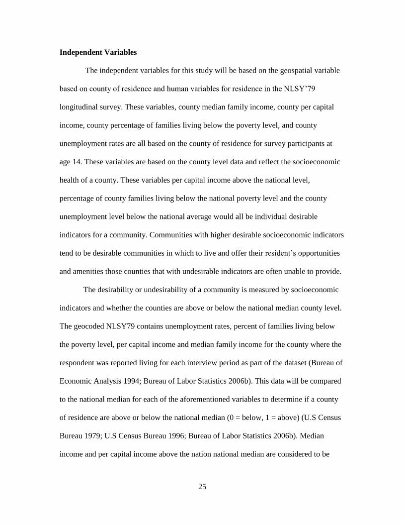
Independent Variables
The independent variables for this study will be based on the geospatial variable
based on county of residence and human variables for residence in the NLSY’79
longitudinal survey. These variables, county median family income, county per capital
income, county percentage of families living below the poverty level, and county
unemployment rates are all based on the county of residence for survey participants at
age 14. These variables are based on the county level data and reflect the socioeconomic
health of a county. These variables per capital income above the national level,
percentage of county families living below the national poverty level and the county
unemployment level below the national average would all be individual desirable
indicators for a community. Communities with higher desirable socioeconomic indicators
tend to be desirable communities in which to live and offer their resident’s opportunities
and amenities those counties that with undesirable indicators are often unable to provide.
The desirability or undesirability of a community is measured by socioeconomic
indicators and whether the counties are above or below the national median county level.
The geocoded NLSY79 contains unemployment rates, percent of families living below
the poverty level, per capital income and median family income for the county where the
respondent was reported living for each interview period as part of the dataset (Bureau of
Economic Analysis 1994; Bureau of Labor Statistics 2006b). This data will be compared
to the national median for each of the aforementioned variables to determine if a county
of residence are above or below the national median (0 = below, 1 = above) (U.S Census
Bureau 1979; U.S Census Bureau 1996; Bureau of Labor Statistics 2006b). Median
income and per capital income above the nation national median are considered to be

26
desirable. The opposite is true of poverty and unemployment rates where a percentage
above the national rates is undesirable for these dependent rates. Then by measuring the
dependent variables as desirable and undesirable the labels are able to transpose to the
variables the socioeconomic rating for the geospatial community.
In addition to these four independent variables cited above additional human
capital and geospatial variables will be examined through binary regression analysis to
determine the variables relationship in influencing the outcomes of migration. These
variables include lifecycle characteristics for the individual respondents. The variables
for Family below the poverty level in 1979 (0 = family not in poverty, 1 family in
poverty), Sex (0 = female, 1= male), race (0 = white and other, 1 = black) and ethnicity (0
= Non Hispanic, 1= Hispanic). Years of school (1 = less than High School, 2 = High
School, 3 = Some College, 4 = four years of college, 5 = greater than 4 years of college)
will provide information on educational levels. Life cycle variables include marital states
(0 = not married, 1 = married), and children at home in 2002 (0 = no children, 1 = 1 child,
2 = 2 children, 3 = three or more children).
Geographic Control
For the geographic variables the research will utilize the United States
Department of Agriculture’s Rural-Urban Continuum Codes. In this study, the codes will
be used to determine if a county is rural or Metro in both measurement periods (0 = non-
metro area of less than 250,000, 1 = metro area greater than 250,000). This variable is
determined by the U.S. Department of Agriculture and is a recognized as the standard for
measuring if a county is a rural or urban county at all levels of government (Economic
Research Service 2003; Economic Research Service 2003; Economic Research Service
27
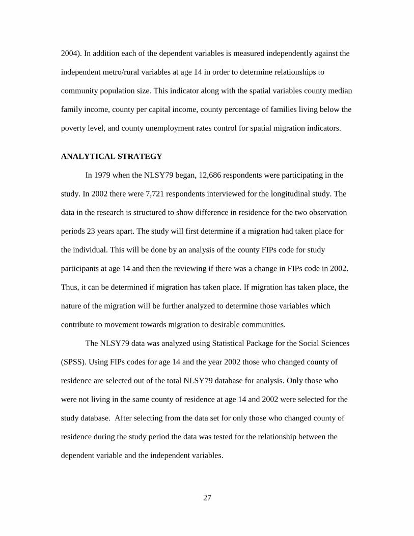
2004). In addition each of the dependent variables is measured independently against the
independent metro/rural variables at age 14 in order to determine relationships to
community population size. This indicator along with the spatial variables county median
family income, county per capital income, county percentage of families living below the
poverty level, and county unemployment rates control for spatial migration indicators.
ANALYTICAL STRATEGY
In 1979 when the NLSY79 began, 12,686 respondents were participating in the
study. In 2002 there were 7,721 respondents interviewed for the longitudinal study. The
data in the research is structured to show difference in residence for the two observation
periods 23 years apart. The study will first determine if a migration had taken place for
the individual. This will be done by an analysis of the county FIPs code for study
participants at age 14 and then the reviewing if there was a change in FIPs code in 2002.
Thus, it can be determined if migration has taken place. If migration has taken place, the
nature of the migration will be further analyzed to determine those variables which
contribute to movement towards migration to desirable communities.
The NLSY79 data was analyzed using Statistical Package for the Social Sciences
(SPSS). Using FIPs codes for age 14 and the year 2002 those who changed county of
residence are selected out of the total NLSY79 database for analysis. Only those who
were not living in the same county of residence at age 14 and 2002 were selected for the
study database. After selecting from the data set for only those who changed county of
residence during the study period the data was tested for the relationship between the
dependent variable and the independent variables.

28
Table 1. Descriptive Statistics for Dependent Variable Measurements Description Mean SD Min Max
County Median Family
Income for the County of
Residence in 2002
County Median Family Income for
Study Participants Above National
Median (0 = Undesirable, 1 =
Desirable)
.58 .494 0 1
Through binary regression the study determines the variables that lead to
migration to desirable counties as opposed to undesirable communities whose median
income is below the national median incomes. The independent variable can be divided
into two distant classifications: those attributes that contribute to an individual’s human
capital, such as sex, race and income, and spatial variable such as rural/urban and county
level socioeconomic measurements that measure the effect of community on the
migration outcomes.
The study then uses cross tabulations to show migration patterns for NLSY’79
participants. The cross tabulation analysis measures the dependent variable desirability
of the median income of county of residence against the independent variable desirability
of the county of residence of the median income of the county of residence at age 14.
Then the additional demographic and geospatial variables are integrated into the analysis.
This creates a layered cross tabulation wherein the demographic and geospatial
independent variables are nested within the main independent variables. The resulting
cross tabulation table allows testing of the secondary independent variable against the
dependent variable and the primary independent variables. Each cross tabulation data set
is tested using chi-square significance tests. Each of the independent variables is tested
against the main dependent variable.

29
Table 2. Descriptive Statistics for Independent Variable Measurements
Description Mean SD Min Max
Gender R is Male (1 = Male, Female 2)) 1.5 .500 1 2
Race R is race (0 = White and Other,
1 = Black)
.312 .463 0 1
Ethnicity R is race/ethnicity ( 0 =
Non Hispanic, 1 = Black)
.162 .368 0 1
Education 2002 R’s Education (1 = Under
High School Education, 2 =
High School Education, 3 =
Some College, 4 Years of
College, 5 = More Than 4
Years of College
2.78 1.282 1 5
Marital Status 2002 R is Married at time t ( 1 =
Never Married, 2 = Married,
Spouse Present, 3 = Other)
.602 .489 0 1
Number of Children at
Home
Number of Children in R
household living at home at
time t (0 = No Dependents,
1 = 1 Dependent, 2 = 2 Dependents
3 = 3 Dependents or More)
1.31 1.114 0 3
Family Poverty Status R is Family Poverty Status (0 = Not
in Poverty, 1 = In Poverty)
.22 .415 0 1
Lived in Rural or
Urban area at 14
R’s County of Residence at age 14
and then in 1979 (0 = Non Metro,
1 = Metro)
.59 .492 0 1
County of Origin
Median Family Income
at Age 14
County Median Family Income for
R’s County of Residence at age 14
(0 = Undesirable, 1 = Desirable)
.44 1. .496 0 1
County of Origin Per
Capital Income at Age
14
County Median Family Income for
R’s County of Residence at age 14
(0 = Undesirable, 1 = Desirable)
.45 , .497 0 1
County of Origin
Percentage of Families
Poverty Level at Age 14
County Percentage of Families
Below the Poverty Level for R’s
County of Residence at age14 (0 =
Undesirable, 1= Desirable)
.519 .499 0 1
County of Origin
Unemployment Rate at
Age 14
County Level of Unemployment for
R’s County of Residence at age 14
(0 = Undesirable, 1 = Desirable)
.549 .497 0 1

30
RESULTS
The NLSY79 data (Table 3) shows that 70% of those participating in the study
have changed county of residence at least one time between age 14 and the 23 years of
age. Of those who moved from county of residence at age 14, 25% were repatriated to
the county of residence at age 14 by the 2002 study period. Study participants living in a
different county of residence from age 14 (Table 5) is 52% for the 2002 interview period.
The total migration from county of residence at age 14 has been a gradual migration with
9.6% to 20.7% of the study participants changing their county of residence in any one
interview period. The data that is available does show that the number of moves for
participants ranged for 1 to 15 county relocations with a 3.27 mean for the inter-county
moves that are accounted for in the NLSY79. The precise number of intra-county moves
can not be accounted for by the NLSY79, because of moves between intervening
interview periods or the interviewers were unable to establish contact with study
participants for a particular study period. When these variables are viewed together they
tend to point to the fact that once an individual has migrated from the county they lived
during adolescence they are unlike to return to that location in successive years.
Table 3. At Least One Change in County of Residence Between Age 14 and 2002 Frequency Percent
Never Moved 2218 30
Move at Least 1 Time 5164 70
Total 7382
31
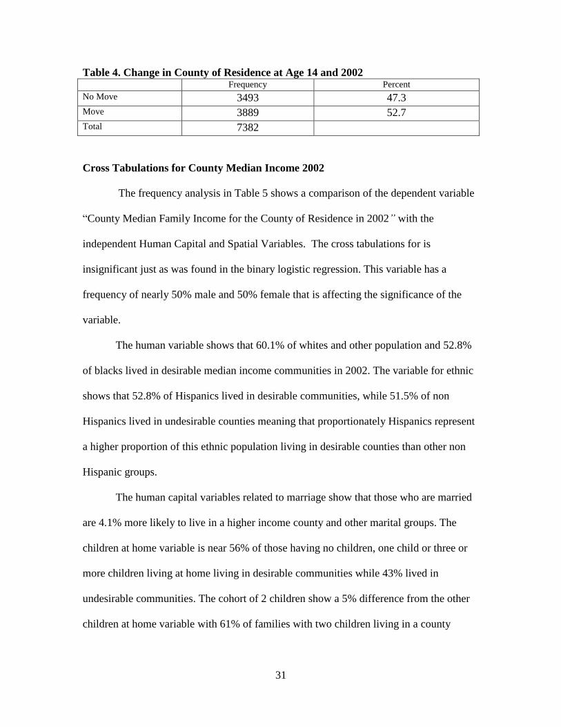
Table 4. Change in County of Residence at Age 14 and 2002 Frequency Percent
No Move 3493 47.3
Move 3889 52.7
Total 7382
Cross Tabulations for County Median Income 2002
The frequency analysis in Table 5 shows a comparison of the dependent variable
“County Median Family Income for the County of Residence in 2002” with the
independent Human Capital and Spatial Variables. The cross tabulations for is
insignificant just as was found in the binary logistic regression. This variable has a
frequency of nearly 50% male and 50% female that is affecting the significance of the
variable.
The human variable shows that 60.1% of whites and other population and 52.8%
of blacks lived in desirable median income communities in 2002. The variable for ethnic
shows that 52.8% of Hispanics lived in desirable communities, while 51.5% of non
Hispanics lived in undesirable counties meaning that proportionately Hispanics represent
a higher proportion of this ethnic population living in desirable counties than other non
Hispanic groups.
The human capital variables related to marriage show that those who are married
are 4.1% more likely to live in a higher income county and other marital groups. The
children at home variable is near 56% of those having no children, one child or three or
more children living at home living in desirable communities while 43% lived in
undesirable communities. The cohort of 2 children show a 5% difference from the other
children at home variable with 61% of families with two children living in a county

32
above the median income in 2002 and 38.9% living in counties below the national
median income level.
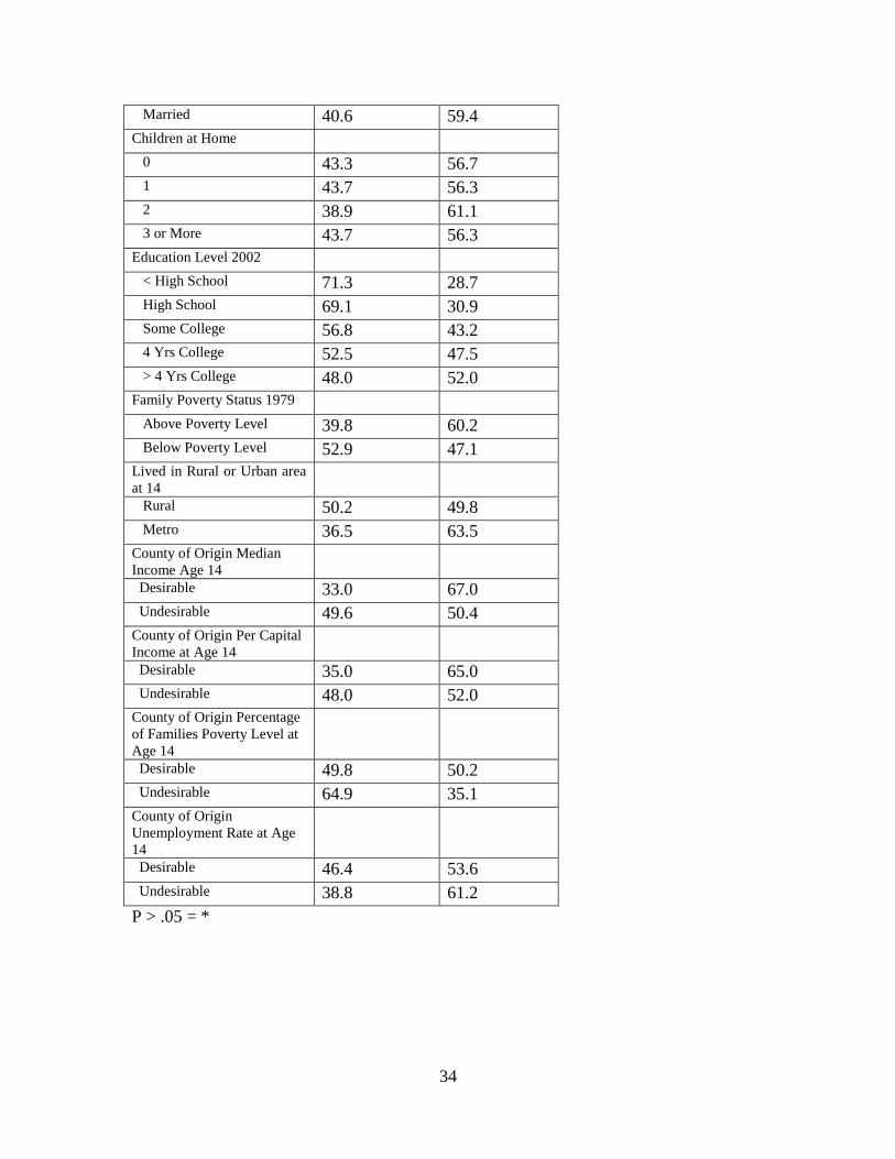
Educational variable show that 71.3% of those with less than a high school and
69.1% of those with educational attainment of a high school degree lived in counties with
a median income below the national median income level. This pattern follows for the
cohorts of some college (56.8%), college degree (52.5%) and graduate or professional
degree (48%) which shows a negative slope as education increases. A positive slope can
be found when comparing less than high school education (28.7%) to greater than 4 years
of college (52%). As the education level increase the study participants were more likely
to live in counties with median incomes above the national level.
The cross tabulation show that the majority of those who live in desirable median
income communities (60.2%) were from families with incomes above the poverty level at
age 14. Those who at age 14 had a family income that was above the poverty level but
lived in counties in the year 2002 with median incomes below the poverty level was
39.8%. Of the population whose family income was below the poverty level at age 14,
47.1% of the population lived in counties with median incomes above the national
median income.
The cross tabulation for geospatial spatial related variables are related to the place
where the study participants lived at 14 years of age. This data show that there is a nearly
even 50/50 split of those who lived in rural areas to move to desirable and undesirable
median income counties in 2002. Those who lived at 14 years of age in a metro area were
more likely to move to a desirable county. Over 63% of this population moved to
desirable counties in 2002 and only 36% moved to undesirable counties. The median

33
income variables for both age 14 and the year 2002 show that 67% of those who lived in
desirable communities at age 14 also lived in desirable communities in 2002. This show
little downward mobility with less than 40% moving to undesirable counties for the
median income variables. The median income variables for those living below the
median income show a nearly 50/50 split between moving to a desirable and undesirable
community in 2002.
Of those living in counties with poverty rates below the national poverty level at
age 14. Nearly 65% lived in counties with median incomes below the national median
income in 2002. Only 35% of this population moved to the desirable median income
counties. For those who live in the desirable counties at age 14 the population was evenly
split between the desirable and undesirable communities. The unemployment data at age
14 shows that overwhelmingly those who migrated from areas of high unemployment
toward counties in 2002 with desirable median incomes. Only 38.8% of this population
migrated to counties with undesirable median incomes.
Table 5. County Median Family Income for the County of Residence in 2002
N = 3830
Undesirable Desirable
Gender *
Male 41.7 58.3
Female 42.7 57.3
Race
White and Other 39.9 60.1
Black 47.2 52 .8
Race/Ethnic
Non Hispanic 51.5 48.5
Hispanic 47.8 52.2
Marital Status
Single, 0ther 44.7 55.3
34
Married 40.6 59.4
Children at Home
0 43.3 56.7
1 43.7 56.3
2 38.9 61.1
3 or More 43.7 56.3
Education Level 2002
< High School 71.3 28.7
High School 69.1 30.9
Some College 56.8 43.2
4 Yrs College 52.5 47.5
> 4 Yrs College 48.0 52.0
Family Poverty Status 1979
Above Poverty Level 39.8 60.2
Below Poverty Level 52.9 47.1
Lived in Rural or Urban area
at 14
Rural 50.2 49.8
Metro 36.5 63.5
County of Origin Median
Income Age 14
Desirable 33.0 67.0
Undesirable 49.6 50.4
County of Origin Per Capital
Income at Age 14
Desirable 35.0 65.0
Undesirable 48.0 52.0
County of Origin Percentage
of Families Poverty Level at
Age 14
Desirable 49.8 50.2
Undesirable 64.9 35.1
County of Origin
Unemployment Rate at Age
14
Desirable 46.4 53.6
Undesirable 38.8 61.2
P > .05 = *

35
Living in an Above the Median Income County in 2002
The results of binary logistic regression analysis are shown in Table 6, Table 7
and Table 8. Table 6 shows the results the dependent “County Median Family Income for
the County of Residence in 2002” relationship when tested against each of the twelve
independent variables. Table 7 shows the results of testing the dependent variable and the
independent variables that are related to human capital and community spatial variables.
The variable “County of Origin Median Income Age 14” was excluded from this table
because of its correlation to the “County Median Family Income for the County of
Residence in 2002”. Table 8 adds the variable “County of Origin Median Income Age
14” to the models so that to test the variables relationship to the human and the other
independent spatial variables.
The binary logistic regression was used to test each of the independent variables
“Marital Status”, “Race”, “Ethnicity”, “Family Poverty Level at 14”, and “Educational
Level 2002” were found to be significant human variables. “Gender” and “Number
Children at Home” were found to be not significant for binary logistic regression. The
spatial variable “Lived in rural or urban area at 14”, “County of Origin Per Capital
Income at Age 14”, “County of Origin Percentage of Families Poverty Level at Age 14”,
“County of Origin Unemployment Rate at Age 14” and “County of Origin Median
Income Age 14” were all found to be significant when binary logistic regression was
used for analysis.

36
Table 6. Binary Logistic Regression - County Median Family Income for the
County of Residence in 2002
County Median Family Income for
the County of Residence in 2002-
Desirable
B S.E
Odds
Ratio Sig
County of Origin Median Income Age
14 - desirable 0.691 0.069 1.997 0.000
Gender-Female -0.040 0.065 0.961 0.544
Marital Status- Married 0.165 0.067 1.180 0.013
Number Children at Home -3 0.026 0.029 1.027 0.371
Race - Black -0.298 0.070 0.742 0.000
Ethnicity - Hispanic -0.340 0.090 0.712 0.000
Family Poverty Level at 14 - In Poverty -0.529 0.080 0.589 0.000
Educational Level 2002 -Graduate
School 0.267 0.027 1.306 0.000
Lived in Rural or Urban area at 14 -
Metro 0.564 0.067 1.768 0.000
County of Origin Per Capital Income at
Age 14 - Above National Per Capital
Income 0.540 0.068 1.716 0.000
County of Origin Percentage of Families
Poverty Level at Age 14 - Below
National Poverty Rate 0.621 0.067 1.860 0.000
County of Origin Unemployment Rate at
Age 14 - Below National
Unemployment Rate 0.307 0.067 1.360 0.000
The result of multivariate logistic regression in Table 7 investigates the
relationship of the human capital and the spatial variables in relationship to the
Dependent Variable median income of county of residence in 2002. The human capital
variables “Gender”, “Marital Status” and “Number of Children at Home” were not
significant to model A. The significance of “Race” is .059 and is slightly above the .05
significance level is slightly above the 95% confidence level. The variables “Ethnicity”,
“Family Poverty Level at 14” and “Educational Level 2002” where found to be
significant. “Race”, “Ethnicity” and “Family Poverty Level at 14” were negatively

37
associated with living in a “Median Family Income for the County of Residence in 2002”
that is desirable. “Educational Level 2002” was positively associated with the “County
Median Family Income for the County of Residence in 2002”. Blacks are .860 less like to
live in a county with median income above the national median income while Hispanics
are .824 less likely. If the family was in poverty at age 14 then it is a .724 less likely that
the individual will live in a county above the median income level. Education was
positively related to the county median income variable. Where family poverty status
made it 26% less like for an individual to live in a county with an income above the
median income, Education increased the chances of living in a county with a median
income above the national median income. Education increases the chances of living in a
desirable median income community by nearly 28%.
“County of Origin Per Capital Income at Age 14”, “County of Origin Percentage
of Families Poverty Level at Age 14”, and “County of Origin Unemployment Rate at Age
14”variable where not significant in Table 6. Model B. The only spatial variable that is
significant in this model was “living in a rural or urban area at 14” and the odds ratio is
1.434. Living in a metro area at age 14 increased the chance, by 43%, for “living in a
county above the median income in 2002”.
38
Table 7. Multivariate Logistic Regression for County Median Family Income for the County of Residence in 2002 Excluding
County of Origin Median Income Age14
County Median Family Income for the County of Residence in 2002
without County of Origin Median Income Age14
Model A Human Variables Model B Spatial Variables
B S.E Odds
Ratio
Sig B S.E Odds
Ratio
Sig
County of Origin Median Income Age
14 - desirable
Gender-Female -0.067 0.070 0.935 0.340
Marital Status- Married -0.052 0.081 0.949 0.519
Number Children at Home -3 0.078 0.035 1.018 0.612
Race - Black -0.151 0.080 0.860 0.059
Ethnicity - Hispanic -0.193 0.096 0.824 0.044
Family Poverty Level at 14 - In Poverty -0.292 0.089 0.746 0.001
Educational Level 2002 -Graduate
School
0.245 0.029 1.278 0.000
Lived in Rural or Urban area at 14 -
Metro
0.361 0.101 1.434 0.000
County of Origin Per Capital Income at
Age 14 - Above National Per Capital
Income
0.084 0.150 1.088 0.575
County of Origin Percentage of
Families Poverty Level at Age 14 -
Below National Poverty Rate
0.164 0.123 1.178 0.182
County of Origin Unemployment Rate
at Age 14 - Below National
Unemployment Rate
0.023 0.091 1.023 0.804
Cox & Sell R Square Model A - .036 Model B - .032
39
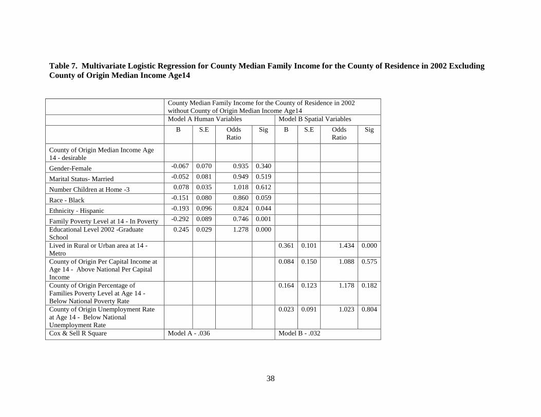
The analysis of the independent variables in Table 7 indicates that the variables
“Race”, “Ethnicity”, “Family Poverty Level at 14”, and “Educational Level in 2002” are
significant human capital and lived in rural or urban area at 14 being the only significant
spatial variables in the multivariate logistic regression in Table 7. In Table 6 “County of
Origin Median Income Age 14” had the highest odd ratio (1.997) associated with
“County Median Family Income for the County of Residence in 2002”. In Table 7 the
multivariate logistic regression is expanded to include the independent variable “County
of Origin Median Income Age 14”.
In Model A the human capital variables are analyzed as in Table 7, Model A with
the addition of the independent spatial variable “County of Origin Median Income Age
14”. With the addition of this new independent variable “Race” is no longer a significant
variable along with the independent variable that were not significant in Table 8, Model
A. Hispanics are -20% less likely to live in a community with a median income above the
national median income level. The odds ratio for “Family Poverty Level at 14” decreases
by 4% with the new odds rations changing from .746 to .785. The association odds ratio
for “Educational Level 2002” varies between the two tables by less than .002. The odds
ratio for “County of Origin Median Income Age 14” has a positive odds ratio of 1.808.
While this independent variable is significant, adding this variable does not improve the
association of human capital variables to “County Median Family Income for the County
of Residence in 2002” found in Table 7.
In Table 8, Model B the independent spatial variable “Lived in Rural or Urban
area at 14” decreases by 8% with the addition of “County of Origin Median Income Age
14”. With the addition of this new variable, however, “County of Origin Unemployment
40
Rate at Age 14” becomes a significant variable, with an odds ratio of 1.203. Like in
Model A, human capital variables, “County of Origin Median Income Age 14” had the
highest odds ratio for the spatial variables selected. Under this model being from a county
at age 14 with a median income above the national median income level, increase by 48%
of living in a county in 2002 of living in a county with a median income level above the
national median income. With the addition of the “County of Origin Median Income Age
14” variable added to the spatial variable Model B, “County of Origin Unemployment
Rate at Age 14” becomes a significant variable with an odds ratio of 1.203. While this
odds ratio for this variable is less than the two other spatial significant variables, it is still
within the range of the human capital variables.
Model C combines the human capital form Model A and the spatial variables
Model B so that the variable from each model can be compared. In this model “County of
Origin Median Income Age 14”, “Lived in Rural or Urban area at 14”, and “County of
Origin Unemployment Rate at Age 14” are the significant spatial variables. The
significant human capital variables are “Ethnicity”, “Family poverty level at 14”, and
“education level 2002”.
The spatial variable “lived in rural or urban area at 14” has an odds ratio of 1.435
which is highest of the six significant variables in this model. Living in a metro area at
age 14 increase the chances of moving to a community with a median income above the
national median income increase. The spatial variable “county of residence at age 14
median” is the second most significant variable under this model. Living in a community
with an above the national median income level increases the chances of living in a
community in 2002 with a median above the national median income by 39%. The third
41
significant spatial variable in this model is “County of Origin Unemployment Rate at Age
14”. Like the preceding spatial variable this is a positive correlation at 1.160. The human
variable “ethnicity” (.806) and “family poverty level at 14” (.803) are negatively
correlated to the dependent variable. Living in poverty and being a member of a Hispanic
ethnic group decrease the chances of living in a county with a median income above the
national median income level. Again the “education level 2002” has a positive correlation
to living in a county with a median income above the national level. As the level of
education increases the chances of living in a county with an above the national median
income level also increases.
The spatial odds for living in a county with an above the national median income
are 16% higher for those who lived in metro area and 12% for those who lived in an
above median income county at 14 than the variable for education level in 2002. In this
model these two variables have a greater influence on living in a higher income county
than education. Ethnicity and living in poverty as a youth decrease the chance of living in
a county above the national median income.

42
Table 8. Multivariate Logistic Regression for County Median Family Income for the County of Residence in 2002 Including
County of Origin Median Income Age14
County Median Family Income for the County of Residence in 2002 with County of Origin Median Income Age14
Model A Human Variables Model B Spatial Variables
Model C Human and Spatial
Variables
B S.E Odds Ratio Sig B S.E Odds Ratio Sig B S.E Odds Ratio Sig
County of Origin Median Income Age14 -
desirable 0.592 0.074 1.808 0.000 0.396 0.137 1.486 0.004 0.334 0.143 1.396 0.020
Gender-Female -0.058 0.072 0.943 0.417 -0.058 0.072 0.943 0.417
Marital Status- Married -0.041 0.083 0.960 0.623 -0.040 0.084 0.961 0.630
Number Children at Home -3 0.017 0.036 1.017 0.640 0.015 0.036 1.015 0.674
Race - Black -0.018 0.084 0.982 0.826 -0.054 0.086 0.947 0.529
Ethnicity - Hispanic -0.218 0.099 0.804 0.027 -0.216 0.101 0.806 0.033
Family Poverty Level at 14 - In Poverty -0.242 0.092 0.785 0.008 -0.219 0.092 0.803 0.018
Educational Level 2002 -Graduate School 0.244 0.030 1.276 0.000 0.245 0.030 1.277 0.000
Lived in Rural or Urban area at 14 - Metro 0.306 0.085 1.357 0.000 0.361 0.090 1.435 0.000
County of Origin Per Capital Income at
Age 14 - Above National Per Capital
Income -0.098 0.107 0.907 0.362 -0.093 0.111 0.911 0.491
County of Origin Percentage of Families
Poverty Level at Age 14 - Below National
Poverty Rate 0.206 0.119 1.228 0.083 0.126 0.127 1.134 0.320
County of Origin Unemployment Rate at
Age 14 - Below National Unemployment
Rate 0.185 0.070 1.203 0.002 0.148 0.075 1.160 0.049
Cox & Sell R Square Model A - .055 Model B - .034 Model C - .061

43
CONCLUSION
The data provides evidence that a higher percentages of individuals from
undesirable communities move to desirable communities meanwhile, individuals from
desirable communities are less likely to move to undesirable communities. For those who
move from desirable to desirable communities the evidence suggests that this movement
is by choice. It can also be assumed that movement from undesirable to desirable is by
choice since these moves can easily be explained though theories relating economics to
migration. Migration to undesirable communities cannot be as easily be explained as
economic migration since the mover is moving from desirable to undesirable or
undesirable to undesirable. Family socio-economic status most does play a significant
role in this migration pattern yet there is evidence that spatial variables also influence this
migration pattern. How the place of residence at age 14 affects migration is beyond the
scope of this study since only a two by two analysis is employed. Through the use of
covariant analysis it would be possible to study further spatial variable affects on
migration.
The variables associated with the place of residence during adolescence
demonstrate that “County of Origin Median Income Age 12”, “County of Origin
Unemployment Rate at Age 14” and “Lived in Rural or Urban area at 14” are associated
with moving to a desirable community. Those who at age 14 resided in an urban area,
from counties with a low unemployment rate and high median income level, are likely to
have moved by middle age to a community with a median income above the national
level. The data illustrates that there is little downward social mobility for those who
44
during adolescence were raised in environments of higher standing. Those variables that
measure higher social status demonstrate that individuals with privilege move to
communities with desirable median incomes.
The portrait of migration that emerges from the NLSY79 data depicts that those
born to privilege live in higher median income communities. Only one-third of this
population is downwardly mobile. Upward mobility for those from lower status
adolescence communities is nearly even with approximately half moving to desirable
communities and the other half moving to undesirable communities. Those with lower
education levels tend to move to undesirable communities with 71% of the respondents
who have less than a high school education living in undesirable communities in 2002.
With lower levels of education, the mover population tends to cluster in undesirable
communities supporting the theory that movers tend to move to homogeneous
communities where individuals of similar status live.
Economic theories of migration hold that individuals migrate for economic reasons.
Migrants when they move tend to minimizing risk and to maximize the opportunities
associated with migration. If migration was based only on economics, moving from
undesirable communities to desirable would be the predominate move. Communities that
have a high income levels provide more as well as better services to their citizens. In such
communities even the poor have a better quality of services than are provided to the
wealthy in undesirable communities. Because of the quality of life in these desirable
communities it would be expected that all movers would move to desirable communities.
The data from the NLSY79, however, explains that those who lived in undesirable
counties at 14 years of age had a 50% rate of moving to counties with a desirable median
45
income level by their middle age. Of the population that moved from desirable counties
of origin, 67% were able to move to another desirable community in 2002. The data
illustrates that there is a tendency to move to desirable communities in 2002 for both
those who lived at age 14 in both desirable and undesirable communities of origin. This
finding supports economic theories of migration that state that migration takes place for
potential economic benefits.
These findings also tend to suggest that the economic and social status of the
community where the study participants lived during adolescence influences the type of
community where they lived later in life. This conclusion must be tempered by the fact
that “Family Poverty Level at 14” for those how lived in poverty is negatively correlated
to being able to move to a desirable community. The data also confirm that education is
positively correlated to moving to a desirable community, meaning that as an individual’s
income level increases their chances improve for living in a community above the
poverty level.
Individual social economic variables in this study point to the premise that
individual social-economic variables influence the location where a mover lives during
middle age since the data shows that those from a family living above the poverty level,
and those with higher educational achievement, have a higher chance of living in a
desirable community than those from families below the poverty level, with low
educational achievement.
46
WORKS CITED
Adelman, Robert M., and Stewart E. Tolnay. 2003. “Occupational Status of Immigrants
and African Americans at the Beginning and End of the Great Migration”
Sociological Perspective 46(2):179-206.
Alexander, J. Trent. 2005. “They’re Never Here More Than a Year: Return migration in
the Southern Exodus, 1940-1970” Journal of Social History 38:653-671.
Allison, Paul D. 1984. Event History Analysis: Regression for Longitudinal Event Data
Sage University Paper, Newbury Park, CA.
Baryla, Edward A., and Douglas Dotterweich. 2001. “Student Migration: Do Significant
Factors Vary by Region?” Education and Economics 9(3):269-280.
Bielby, William T., and Denis D. Bielby. 1992. “I will Follow Him: Family Ties,
Gender-Role Beliefs and Reluctance to Relocate for a Better Job” The American
Journal of Sociology 97(5)1241-1267.
Blau, Peter M., and Otis Dudley Duncan 1967. The American Occupational Structure,
Free Press
Borjas, George J., Stephen G Wronars and Stephen J. Trejo. 1990. “Self-Selection and
Internal Migration in the United States” Discussion Paper, National Longitudinal
Surveys, United States Department of Labor, Bureau of Labor Statistics, NLS 92-
14.
Braswell, Cara Mia, and Robert W. Gottesman. 2001. “Analysis of Factors Influencing
Employment Migration of Recent Degree Recipients” Auburn University, Paper
Presented at the 41st Annual Forum of the Association for Institutional Research,
Long Beach, CA, June 3-4, 2001.
Bureau of Economic Analysis. 1994. Local Area Personal Income 1969-92. Washington
DC: United States Department of Commerce.
Bureau of Labor Statistics. 2006. NLSY79 User’s Guide: A Guide to the 1979-2004
National Longitudinal Survey of Youth Data. Columbus Ohio, Prepared for the
U.S. Department of Labor by Center for Human Resource Research, The Ohio
State University, Columbus, Ohio. United States Department of Commerce.
Bureau of Labor Statistics. 2006. “National Longitudinal Surveys, All Cohorts, May
2006, CDrom U.S Department of Labor, United States Department of Commerce.
Available: NLS User Services 614-442-7366.
Cadwallader, Martin. 1992. Migration and Residential Mobility: Macro and Micro
Approaches, Madison, Wisconsin: University of Wisconsin Press.

47
Chriswick, Berry R. 2000. “Are Immigrants Favorably Self-Selected? An Economic
Analysis” Discussion Paper 131, University of Illinois at Chicago and Institute for
the Study of Labor Boon, Germany.
Cotė, Guy L. 1997. “Socio-Economic Attainment, Regional Disparities, and Internal
Migration” European Sociological Review 13(1):55-77.
Cushing, Brian. 2003. “State Minimum Wage Laws and the Migration of the Poor”
Regional Research Paper 2003-3, West Virginia University, Morgantown WV.
DaVanzo, Julie. 1983. “Repeat Migration in the United States: Who Moves Back and
Who Moves On?” The Review of Economics and Statistics 65(4):552-559.
Duncan, Cynthia M. 1992 Worlds Apart: Why Poverty Persists in Rural America, New
Haven CT: Yale University Press.
Economic Research Service. 2003. “Measuring Rurality: What is Rural?” Washington,
DC: United States Department of Agriculture. Retrieved 10/3/2006.
Economic Research Service. 2003. “Measuring Rurality: Urban Influence Codes”
Washington, DC: United States Department of Agriculture. Retrieved 10/3/2006
Economic Research Service. 2004. “Measuring Rurality: Rural-Urban Continuum Codes”
Washington, DC: United States Department of Agriculture. Retrieved 10/3/2006
Fulton, John A., and Glenn V. Fuguitt, Richard M. Gibson. 1997. “Recent Changes in
Metropolitan-Nonmetropolitan Migration Streams” Rural Sociology 62(3):363-
384.
Frazis, Harley J., and James R. Speletzer. 2005. “Worker Training: What We’ve Learned
from the NLSY79” Monthly Labor Review February pp. 48-58.
Frey, William H. 2004. “The New Great Migration: Black Americans’ Return to the
South 1965-2000” The Living Cities Series, The Brookings Institution May, 2004.
Frey, William H., and Kao-Lee Liaw. 2005. Interstate Migration of Hispanics, Asians and
Blacks: Cultural Constraints and Middle Class Flight” Population Studies Center,
Report 05-5, May 2005, Population Studies Center, University of Michigan
Institute for Social Research.
48
Goetz, Stephen J. “Migration and Local Labor Markets” The Web Book of Regional
Science, Regional Research Institute, West Virginia University. Accessed at
http://www.rri.wvu.edu/WebBook/Goetz/. October 3, 2005.
Greenwood, Michael J. 1975. “Simultaneity Bias in Migration Models: An Empirical
Examination” Demography 12(3):521-544.
Greenwood Michael J. 1975. “Research on Internal Migration in the United States: A
Survey” Journal of Economics 13(2):397-433.
Greenwood, Michael J. 1985. “Human Migration: Theory, Models and Empirical
Studies” Journal of Regional Science 25(4):521-544.
Greenwood, Michael J., and Patrick J. Gormely. 1971. “A Comparison of the
Determinants of White and Nonwhite Interstate Migration” Demography
8(1):141-155
Greenwood, Michael J., Gary L. Hunt, Dan S. Rickman, and George I. Treyz. 1991.
“Migration, Regional Equilibrium and the Estimation of Compensating
Differentials” The American Economic Review 81(5):1382-1390.
Gurak, Douglas T., and Mary M. Kritz. 2000. “The Interstate Migration of U.S.
Immigrants: Individual and Contextual Determinates” Social Forces 73(3):1017-
1039.
Haurin, Donald R., and Jean R Haurin. 1988. “Net Migration, Unemployment, and the
Business Cycle” Journal of Regional Science 28(2):239-254.
Heuer, Ruth E. 2004. “Migration of Recent College Graduates” Ph.D. dissertation,
Department of Sociology, North Carolina State University, Raleigh, NC.
Huang, Tzu-Ling, Peter F. Prazem, and Darin Wohlgemuth. 2002. “Rural Population
Growth, 1950-1990: The Role of Human Capital, Industry Structure and
Government Policy” American Journal Agricultural Economics August
2002:615-627.
Kodrzycki, Yolamda L. 2001. “Migration of Recent College Graduates: Evidence from
the National Longitudinal Survey of Youth” New England Economic Review
January/February.
Kramer, Judith R. 1970. The American Minority Community, Thomas Y. Crowell
Company, New York, NY.
Lee, Everett S. 1966. “A Theory of Migration” Demography 3(1):47-57.
49
Lee, Seong Woo, and Curtis C. Roseman. 1999. “Migration Determinates and
Employment Consequences of White and Black Families 1985-1990” Economic
Geography 75(2):109-133.
Lin, Nan. 2001. Social Capital A Theory of Social Structure and Action Cambridge
University Press New York, NY.
Logan, John R. 1978. “Growth, Politics and the Stratification of Places” The Journal of
Sociology 84(2):404-416.
Logan, John R., and Richard D. Alba, Tom Mcnulty, Brian Fisher. 1996. “Making a
Place in the Metropolis: Locational Attainment in Cities and Suburbs”
Demography 33(4):443-455.
Logan, John R., and Harvey L. Molotch. 1987. Urban Fortunes: The Political Economy
of Place. Berkeley: University of California Press.
Massey, Douglas S. 1990. “Social Structure, Household Strategies and the Cumulative
Causation of Migration” Population Index 56(1):3-36.
Mangalam, J. J. and Harry K Schwarzweller. 1968. General Theory in the Migration:
Current Needs and Difficulties” International Migration Review 3(1):3-18.
Massey, Douglas S. 1996. “The Age of Extremes: Concentrated Affluence and Poverty in
the Twenty-First Century” Demography 33(4):395-412.
Massey, Douglas S., and Nancy A Denton. 1985. “Spatial Assimilation as a
Socioeconomic Outcome” American Sociological Review 50(1):94-106.
Mincer, Jacob. 1978. “Family Migration Decisions” The Journal of Political Economy
86(5):749-773.
Obermiller, Phillip J., and Steven R Howe. 2000. “Moving Mountains: Appalachian
Migration Patterns 1995-2000” Journal of Appalachian Studies 10(3):359-371.
Obermiller, Phillip J., and Steven R. Howe. 2001. “New Paths and Patterns of
Appalachian Migration 1975-1990” Journal of Appalachian Studies 7(2):331-349.
Obermiller, Phillip J., and Steven R. Howe. 2004. “Appalachian Migration Pattern 1975-
1980 and 1985-1990” Appalachian Regional Commission, Washington DC.
Obermiller, Phillip J., and Michael E. Maloney. 2002. Appalachian Social Context Past
and Present Kendall/Hunt Publishing Company.
Parsons, Talcott. 1951. The Social System, New York, McGraw-Hill.

50
Ravenstein, E.G. 1885. “Laws of Migration.” Journal of the Statistical Society XLVII,
Part II:167-235.
Ravenstein, E.G 1989. “The Laws of Migration” Journal of the Royal Statistical Society
52(2):241-305.
Schwarzweller, Harry K., James S. Brown and J.J. Mangalam. 1971. Mountain Families
in Transition; A Case Study of Appalachian Migration, University Park, PA, The
Pennsylvania State University Press.
Seyfrit, Carol L. 1986. “Migration Intention of Rural Youth: Testing an Assumed Benefit
of Rapid Growth” Rural Sociology 51(2):1040-1084.
Sjaastad, L.A, 1962. “The Costs and Returns of Human Migration” Journal of Political
Economy 70:80-83.
South, Scott J. and Kyle D Crowder. 1997. “Escaping Distressed Neighborhoods:
Individual, Community, and Metropolitan Influences” American Journal of
Sociology 102:1040-1084.
Spitze, Glenna. 1984. “Black Family Migration and Wives’ Employment” Journal of
Marriage and the Family 46(4):781-790.
Tickamyer, Ann R. and Cynthia M. Duncan. 1990. “Poverty and Opportunity Structure in
Rural America” Annual Review of Sociology 16:67-87.
Todaro, M. P. 1969. “A Model of Labor Migration and Urban Unemployment in Less
Developed Countries” American Economic Review 59(1):138-148.
Tönnies, Ferdinand. 2002. Community and Society Dover Mineola, New York.
Tolnay, Stewart E., Robert M. Adelman, Kyle D. Crowder. 2002. “Race, Regional Origin
and Residence in Northern Cities at the Beginning of the Great Migration”
American Sociological Review 67(3):456-475.
U.S Census Bureau. 1979. 1977 County and City Data Book United States Census
Bureau, United States Department of Commerce Washington DC.
U.S Census Bureau. 1996. 1994 County and City Data Book United States Census
Bureau, United States Department of Commerce Washington DC.
U.S Census Bureau. 2004. “Geographical Mobility: 2002-2003 Census 2003” Population
Characteristics P20-549 United States Census Bureau, United States Department
of Commerce Washington DC.

51
U.S. Census Bureau. 2005. “Areas with Concentrated Poverty: 199” Census 2000
Special: Reports Censr-16 United States Census Bureau, United States
Department of Commerce Washington DC.
U.S. Census Bureau. 2005. “Income, Earnings and Poverty from the 2004 American
Community Survey” Census 2000 Special; Reports Censr-16 United States
Census Bureau, United States Department of Commerce Washington DC.
Weber, Max, W.G. Runciman, E. Matthews 1978. Max Weber: Selections in Translation
Cambridge University Press, Cambridge UK.
Wenk, Dee Ann, Constance Hardesty. 1993. “The Effects of Rural-to-Urban
Migration on the Poverty Status of Youth in the 1980’s” Rural Sociology
58(1):76-92.
Wilson, William Julius. 1996. When Work Disappears. The World of the New Urban
Poor, Vintage.
Wright, Richard, Mark Ellis, and Virginia Parks. 2005. “Re-placing Whiteness in Spatial
Assimilation Research” City & Community 4(2):111-135.
Yaukey, David, Douglas L. Anderton, Jennifer Hickes Lundquist. 2007. Demography,
The Study of Human Population. Long Grove, IL, Westland Press.
Zimmerman, Carle C., Merle E. Frampton, 1935. Family and Society, New York, D. Van
Nostrand Company.