COMP 6838 Data Mining

LECTURE 5: Data preprocessing: Data Reduction-

Dimension Reduction

Dr. Edgar AcunaDepartment of Mathematics

University of Puerto Rico- Mayaguez

math.uprm.edu/~edgar

Data Reduction

Data AggregationReduction of Dimensionality.DiscretizationNumerosity reduction o Instance selectionData Compression

Dimension ReductionFeature Selection: The main aim of doing feature selection is to reduce the dimensionality of the feature space, by selecting relevant and no redundant features and then removing the remaining irrelevant features. That is, feature selection selects “q" features from the entire set of “p" features such that q ≤ p. Ideally q <<< p.

Feature Extraction: A smaller set of features is constructed by applying a linear (or nonlinear) transformation to the original set of features. The best known method is principal components analysis (PCA). Others: PLS, Principal curves.

Feature selection

We will consider only supervised classification problems.

Goal: Choose a small subset of features such that:

a) The accuracy of the classifier on the dataset does not decrease in a significant way.b) The resulting conditional distribution of a class C, given the selected vector feature G, is as close as possible to the original conditional distribution given all the features F.

o The computational cost of the classification will be reduced since the number of features will be less than before.

o The complexity of the classifier is reduced since redundant and irrelevant features are eliminated.

o It helps to deal with the “curse of dimensionality” effect.

Advantages of feature selection

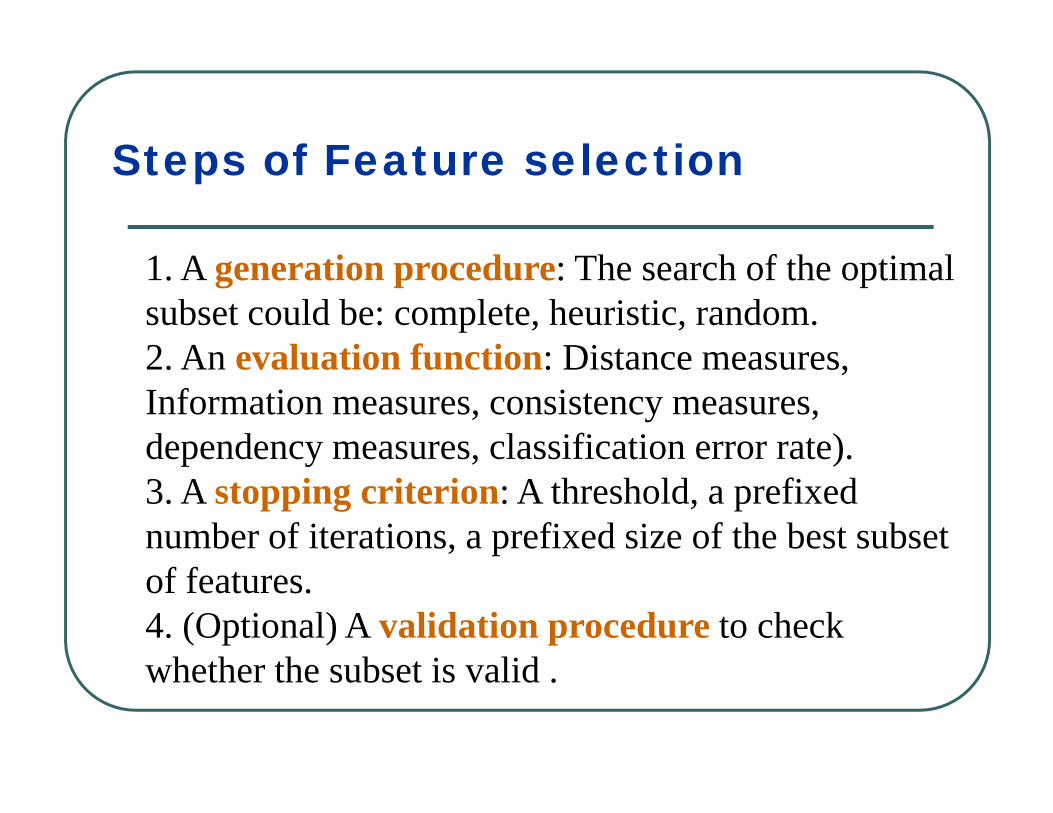
Steps of Feature selection

1. A generation procedure: The search of the optimal subset could be: complete, heuristic, random.2. An evaluation function: Distance measures, Information measures, consistency measures, dependency measures, classification error rate).3. A stopping criterion: A threshold, a prefixed number of iterations, a prefixed size of the best subset of features.4. (Optional) A validation procedure to check whether the subset is valid .

Guidelines for choosing a feature selection method

Ability to handle different types of features (continuous, binary, nominal, ordinal)Ability to handle multiple classesAbility to handle large datasets.Ability to handle noisy data.Low complexity time.

Categorization of feature selection methods (Dash and Liu, 1997)

Generation Evaluation Measures Heuristic Complete Random

Distance Relief

Branch and Bound

-

Information Trees MDL -

Dependency POEIACC - -

Consistency FINCO Focus LVF

Classifier Error rate

SFS, SBS,SFS

Beam Search

Genetic Algorith

The methods in the last row are also known as the “wrapper” methods.

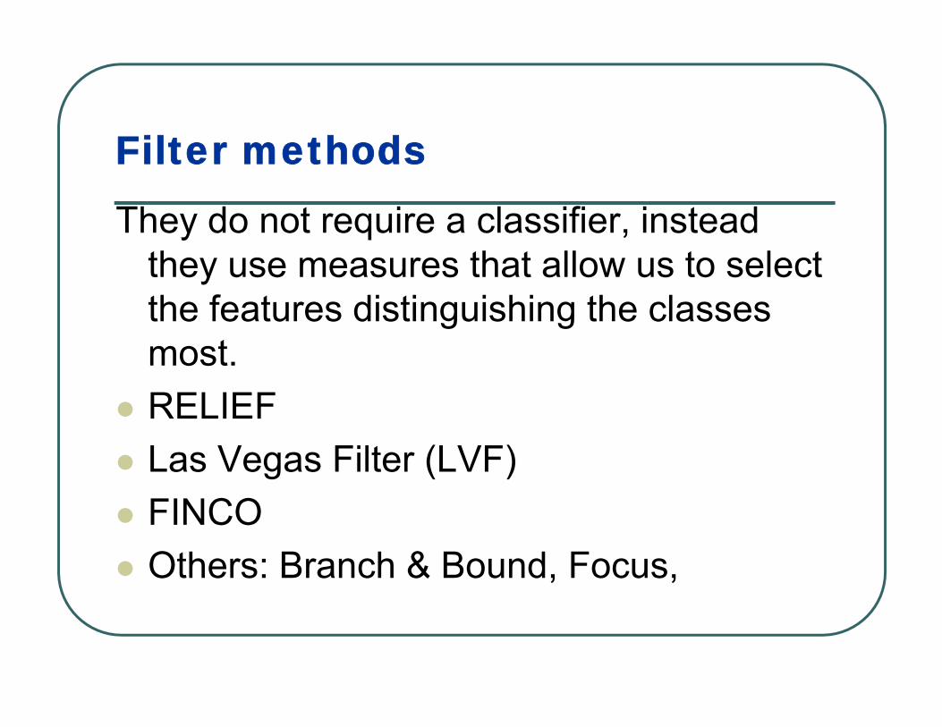
Filter methods

They do not require a classifier, instead they use measures that allow us to select the features distinguishing the classes most.RELIEFLas Vegas Filter (LVF)FINCOOthers: Branch & Bound, Focus,

The RELIEF method

Kira and Rendell (1992) for two-class problem and generalized to multi-class problems by Kononenko (1994) and Kononenko, et al. (1997).Generates subsets of features heuristically.A feature has a relevance weight that is large if it can clearly distinguish two instances belonging to different classes but not two instances that are in the same class. Use a distance measure (Euclidean, Manhattan)

The RELIEF method (procedure)

A given number Nsample of instances are selected randomly from the training set D containing F features.The relevance’s weight Wj of each feature is initialized to zero.For each instance x selected, one must identify two particular instances:Nearhit: The instance closest to x that belongs to its same class.Nearmiss: The instance closest to x that belongs to a different class.

The RELIEF method (distances)

Then the weigths Wj’s (i=1,..F) are updated using the relation

Wj = Wj- diff(xj, Nearhitj)2/NS+ diff(xj, Nearmissj)2/NS

If the feature Xk is either nominal or binary then• diff(xik,xjk) =1 for xik ≠xjk

=0 for the contrary case.If the feature Xk is either continuous or ordinal then:

• diff(xik,xjk) = (xik-xjk)/ck , where ck =range(Xk)

Decision: If Wj≥ τ (a prefixed threshold) then the feature fjis selected

Breast-Wisconsin dataset699 instances, 9 features and two classes (benign or malign). 16 instances have been deleted because contain missing values.1. Clump Thickness 2. Uniformity of Cell Size, 3. Uniformity of Cell Shape, 4. Adhesion Marginal Adhesion, 5. Single Epithelial Cell Size, 6. Bare Nuclei, 7. Bland Chromatin 8. Normal. nucleoli 9. Mitoses. Each feature has values ranging from 0 to 10.

Example of Relief: Breastw

> relief(breastw,600,0)Features appearing in at least half of repetitions ordered by their

average relevance weight: feature frequency weight

[1,] 6 10 0.10913169[2,] 4 10 0.05246502[3,] 1 10 0.04682305[4,] 9 10 0.03171399[5,] 2 10 0.02869547[6,] 3 10 0.02566461[7,] 5 10 0.02512963[8,] 7 10 0.02096502[9,] 8 10 0.01708025selected features [1] 6 4 1 9 2 3 5 7 8> relief(breastw,600,0.04)Features appearing in at least half of repetitions ordered by their

average relevance weight: feature frequency weight

[1,] 6 10 0.10844239[2,] 4 10 0.05293210[3,] 1 10 0.04853909selected features [1] 6 4 1>

Example of Relief: Bupa

> relief(bupa,345,0.0003)Features appearing in at least

half of repetitions ordered by their average relevance weight: feature frequency weight

[1,] 6 6 0.0021190217[2,] 3 8 0.0009031895[3,] 4 8 0.0005711548selected features [1] 6 3 4>

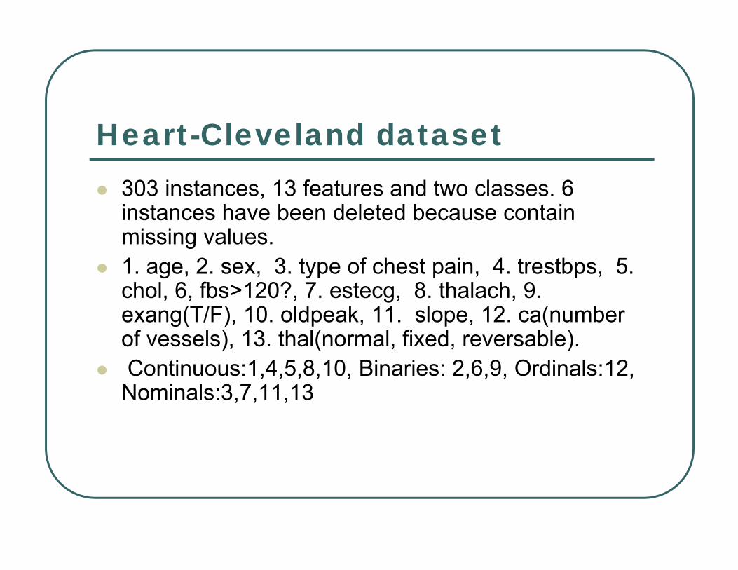
Heart-Cleveland dataset303 instances, 13 features and two classes. 6 instances have been deleted because contain missing values.1. age, 2. sex, 3. type of chest pain, 4. trestbps, 5. chol, 6, fbs>120?, 7. estecg, 8. thalach, 9. exang(T/F), 10. oldpeak, 11. slope, 12. ca(number of vessels), 13. thal(normal, fixed, reversable). Continuous:1,4,5,8,10, Binaries: 2,6,9, Ordinals:12, Nominals:3,7,11,13

Example:Heart-Cleveland

grelief(heartc,297,0.05,v=c(3,7,11,13))Features appearing in at least half of repetitions ordered by their average relevance weight:

feature frequency weight[1,] 13 10 0.60101010[2,] 11 10 0.51582492[3,] 7 10 0.46060606[4,] 3 10 0.45521886[5,] 2 9 0.12356902[6,] 9 9 0.09124579[7,] 12 7 0.05574261selected features [1] 13 11 7 3 2 9 12>

The refief method: multiclass problem

First a Nearmiss has to be found for each class different from x, and then their contribution is averaged using weights based on priors. The weights are updated using:

∑≠ −

+−=

)(

2

2

))(Nearmiss,())((1

)()Nearhit,(

jxclassCj

j

jjj

CxdiffxclassP

CPxdiffWW

Vehicle dataset846 instances, 18 continuous features and four classes(double decker bus, Cheverolet van, Saab 9000 and an Opel Manta 400).[,1] Compactness [,2] Circularity [,3] Distance Circularity [,4] Radius ratio [,5] p.axis aspect ratio [,6] max.length aspect ratio[,7] scatter ratio [,8] elongatedness [,9] pr.axis rectangularity [,10] max.length rectangularity [,11] scaled variance along major axis[,12] scaled variance along minor axis[,13] scaled radius of gyration[,14] skewness about major axis[,15] skewness about minor axis[,16] kurtosis about minor axis[,17] kurtosis about major axis[,18] hollows ratio.

relief(vehicle,400,0.012)Features appearing in at least half of repetitions ordered by their average relevance weight:

feature frequency weight[1,] 16 10 0.03375733[2,] 18 10 0.03087840[3,] 15 10 0.01991083[4,] 17 10 0.01586413[5,] 10 10 0.01521946[6,] 12 9 0.01433016[7,] 9 9 0.01372653[8,] 3 10 0.01369564[9,] 1 9 0.01337022[10,] 7 8 0.01278588[11,] 8 8 0.01267531[12,] 2 5 0.01201989selected features [1] 16 18 15 17 10 12 9 3 1 7 8 2

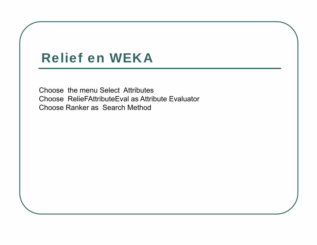
Relief en WEKA

Choose the menu Select AttributesChoose RelieFAttributeEval as Attribute EvaluatorChoose Ranker as Search Method

The Relief method (Cont)

Advantages:It works well for noisy and correlated features.Time complexity is linear on the number of features and on Nsample.It works for any type of feature.Disadvantages:Removes irrelevant features but does not remove redundant features.Choice of the threshold.Choice of the Nsample.

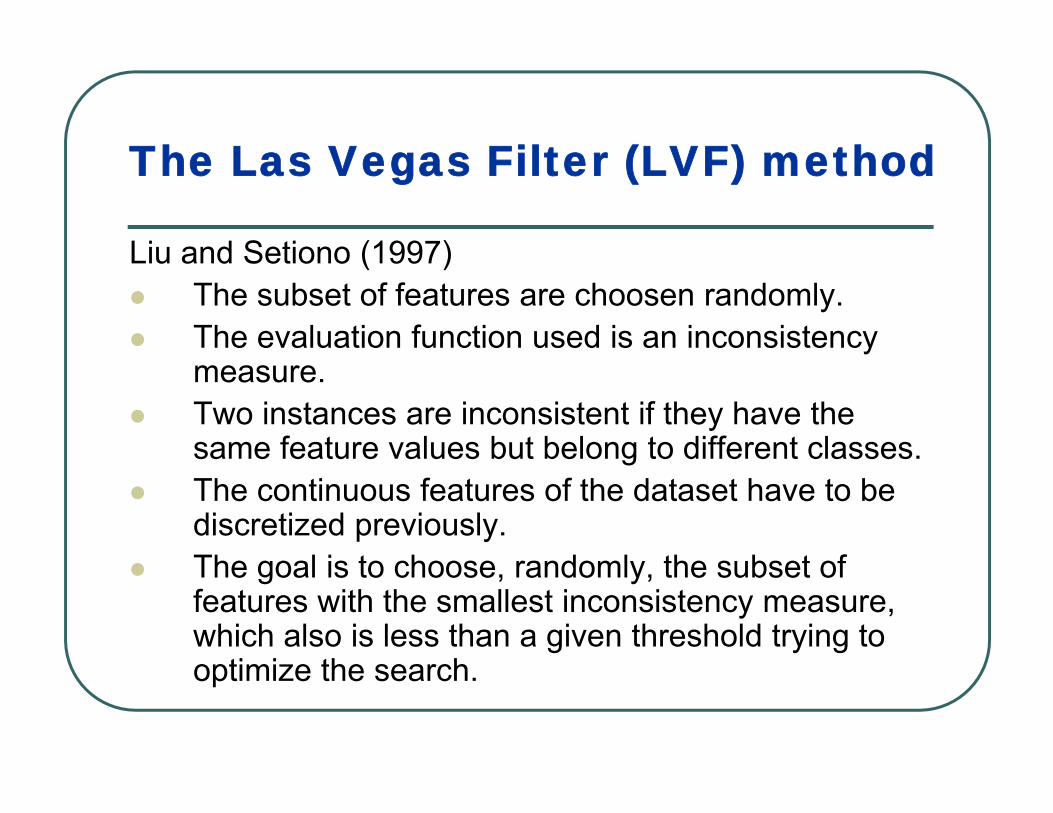
The Las Vegas Filter (LVF) method

Liu and Setiono (1997)The subset of features are choosen randomly.The evaluation function used is an inconsistencymeasure.Two instances are inconsistent if they have thesame feature values but belong to different classes.The continuous features of the dataset have to bediscretized previously.The goal is to choose, randomly, the subset of features with the smallest inconsistency measure, which also is less than a given threshold trying tooptimize the search.

The Inconsistency measureThe inconsistency of a dataset with only

non-continuous features is given by

K: number of the different combinations of the N instances

|Di|: Cardinality of the the i-th combination.hi: frecuency of the modal class on the i-th

combination

N

hDK

iii∑

=−

1||

Inconsistency example> m1

col1 col2 col3 col4 class[1,] 1.5 2 2.0 1 1[2,] 4.0 3 2.1 2 2[3,] 4.0 3 2.1 2 1[4,] 1.5 3 7.9 1 1[5,] 8.9 3 1.3 2 2[6,] 8.9 3 7.9 1 2[7,] 8.9 3 1.3 2 1> inconsist(m1)[1] 0.2857143>

Here K=5, D1=1, D2=2, D3=1 D4=2 and D5=1. Also,h1=…h5=1. Therefore, inconsist=2/7

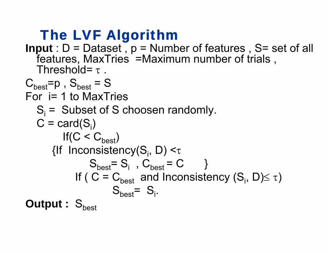
The LVF AlgorithmInput : D = Dataset , p = Number of features , S= set of all

features, MaxTries =Maximum number of trials , Threshold= τ .

Cbest=p , Sbest = SFor i= 1 to MaxTries

Si = Subset of S choosen randomly.C = card(Si)

If(C < Cbest){If Inconsistency(Si, D) <τ

Sbest= Si , Cbest = C }If ( C = Cbest and Inconsistency (Si, D)≤ τ)

Sbest= Si.Output : Sbest

> dbupa=disc.ew(bupa,1:6)> dbupa[1:10,]

V1 V2 V3 V4 V5 V6 V71 10 8 5 5 2 1 12 10 5 6 6 1 1 23 10 4 4 3 3 1 24 13 7 4 4 2 1 25 11 6 1 5 1 1 26 16 4 1 3 1 1 27 11 5 2 3 1 1 18 11 5 2 2 1 1 19 13 4 2 4 1 1 110 12 5 3 3 1 1 1>inconsist(dbupa)[1] 0.01159420> lvf(dbupa,.1,1000)The inconsistency of the best subset is0.05217391The best subset of features is:[1] 1 2 3 6>

More examples> lvf(breastw,.01,2000)The inconsistency of the best subset is0.005856515The best subset of features is:[1] 1 6 8

>

Disadvantages of LVF

Choice of threshold. A small threshold will imply the selection of a larger number of features.A large number of iterations decreases the variability of the chosen subset but it slow down the computation.

The FINCO method

FINCO (Acuna, 2002) combines a sequential forward selection with an inconsistency measure as evaluation function

PROCEDUREThe best subset of features T is initialized as the empty set.In the first step, the feature that produces the smallest level of inconsistency is selected.Then the feature that along with the first feature selected produces the smallest level of inconsistency is selected.The process continues until every feature not yet selected along with the features already in T produces a level of inconsistency less than a prefixed threshold τ.

The FINCO algorithmInput : D = Dataset , p = Number of features in D,

S =set of features of all features , Threshold = τ .Initialization: Set k=0 and Tk= φInclusion: For k=1 to pSelect the feature x+ such that:

where S- Tk is the subset of features not yet selected.If Incons(Tk+x+)<Incons(Tk) and Incons(Tk+x+)>τ, then

Tk+1= Tk+ x+ and k:=k+1else stop Output: Tk: subset of selected features

)(minarg xkTInconskTSx

x +−∈

+ =

Examples> finco(dbupa,.05)features selected and their inconsistency rates$varselec[1] 2 1 6 3$inconsis[1] 0.37681159 0.26376812 0.13333333 0.05217391> finco(breastw,.01)features selected and their inconsistency rates$varselec[1] 2 6

$inconsis[1] 0.07027818 0.02635432

finco(breastw,.001)features selected and their inconsistency rates$varselec[1] 2 6 1

$inconsis[1] 0.070278184 0.026354319 0.005856515

The threshold is a value a little bit larger than the inconsistency of the whole dataset.

LVF and Finco in WEKA

Choose the menu Select AttributesChoose ConsistencySubsetEval as Attribute EvaluatorChoose Random Search as Search Method for LVF andChoose BestFirst as Search Method for FINCO.

Wrapper methodsWrappers use the misclassification error

rate as the evaluation function for the subsets of features. Sequential Forward selection (SFS)Sequential Backward selection (SBS)Sequential Floating Forward selection (SFFS)Others: SFBS, Take l-remove r, GSFS, GA, SA.

Sequential Forward Selection (SFS)

Initially the best subset of features T is set as the empty set.The first feature entering T is the one with the highest recognition rate with a given classifier.The second feature entering T will be the one that along with the feature selected in the previous step produces the highest recognition rate.The process continues and in each step only one feature enters T until the recognition rate does not increase when the classifier is built using the features already in T plus each of the remaining features.

Examples: Bupa and Breastwsfs(bupa,"knn") #knn classifierThe best subset of features is:[1] 5 3 1> sfs(bupa,"lda") #Linear discriminant classifierThe best subset of features is:[1] 5 4 3 6> sfs(bupa,"rpart") #decision tree classifierThe best subset of features is:[1] 5 3 2> sfs(breastw,"knn")The best subset of features is:[1] 6 1 3 7> sfs(breastw,"lda")The best subset of features is:[1] 6 2 1 4> sfs(breastw,"rpart")The best subset of features is:[1] 6 3 5>

Recognition rate versus the number of features being selected by SFS with the Kernel classifier

5 10 15

number of features

0.50

0.55

0.60

0.65

0.70

reco

gniti

on ra

te

Vehicle

5 10 15

number of features

0.29

00.

295

0.30

0

reco

gniti

on ra

te

Segment

5 10 15 20

number of features

0.72

0.73

0.74

0.75

0.76

reco

gniti

on ra

te

German

0 10 20 30 40 50 60

number of features

0.75

0.80

0.85

0.90

reco

gniti

on ra

te

Sonar

Sequential Backward selection(SBS)

Initially the best subset of features T include all the features of the datasetIn the first step we perform the classification without considering each of the feature, and we remove the feature where the recognition rate is the highest.The procedure continues removing one variable in each step until the recognition rates starts to decrease.

No efficient for nonparametric classifiers because has a high computing running time.

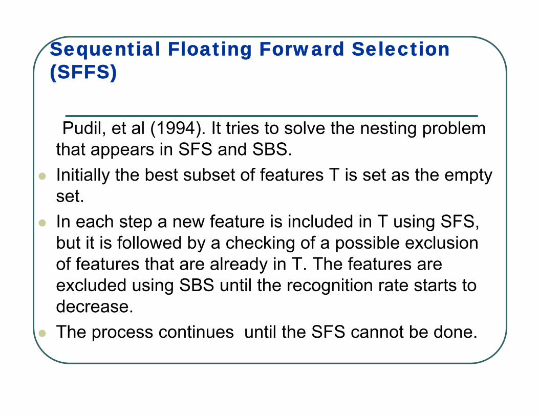
Sequential Floating Forward Selection (SFFS)

Pudil, et al (1994). It tries to solve the nesting problem that appears in SFS and SBS.Initially the best subset of features T is set as the empty set.In each step a new feature is included in T using SFS, but it is followed by a checking of a possible exclusion of features that are already in T. The features are excluded using SBS until the recognition rate starts to decrease.The process continues until the SFS cannot be done.

Examples> sffs(bupa,"lda")The selected features are:[1] 3 4 5> library(class)> sffs(bupa,"knn")The selected features are:[1] 5 3> library(rpart)> sffs(bupa,"rpart")The selected features are:[1] 3 5 6 2> sffs(breastw,"lda")The selected features are:[1] 1 2 6 4> sffs(breastw,"knn")The selected features are:[1] 6 3 7 1> sffs(breastw,"rpart")The selected features are:[1] 6 3 2

Wrappers in WEKA

Choose the menu Select AttributesChoose ClassifierSubsetEval as Attribute EvaluatorChoose BestFirst as Search Method

Experimental MethodologyAll the feature selection methods were applied to twelve datasets available in the Machine Learning Databases Repository at the Computer Science Departament of the Universidad de California, Irvine. Programs for all the algorithms were created in R.The feature selection procedures were compared in two aspects:1. The percentage of features selected.2. The misclassification error rate using the classifiers: LDA, KNN and Rpart.

Methodology for WRAPPERS methods

The experiment was repeated 10 times for datasets with a small number of features. For other cases the experiment was repeated 20 times.The size of the subset was determined by the average number of features selected on all the repetitions.The features selected were those with the highest frecuency.To break ties for the last feature to be selected we assigned weights to the features according to the their selection order.

Methodology for filter methods

In RELIEF and LVF the experiment was repeated 10 times for datasets with an small number of features. For other cases the experiment was repeated 20 times.In RELIEF, the parameter Nsample was taken equal to the number of instances of the dataset.In LVF, the number of subsets selected randomly was chosen between 100 and 5000, and the inconsistency level was selected between 0 and 0.15 depending on the dataset.In FINCO, the experiment was performed only one time and the consistency level was selected between 0 and 0.10 depending on the dataset.

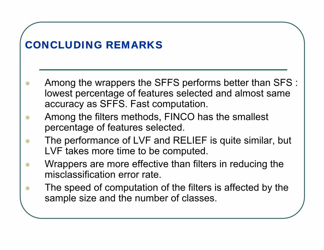
CONCLUDING REMARKS

Among the wrappers the SFFS performs better than SFS : lowest percentage of features selected and almost same accuracy as SFFS. Fast computation.Among the filters methods, FINCO has the smallest percentage of features selected.The performance of LVF and RELIEF is quite similar, but LVF takes more time to be computed.Wrappers are more effective than filters in reducing the misclassification error rate.The speed of computation of the filters is affected by the sample size and the number of classes.

CONCLUDING REMARKS (Cont.)

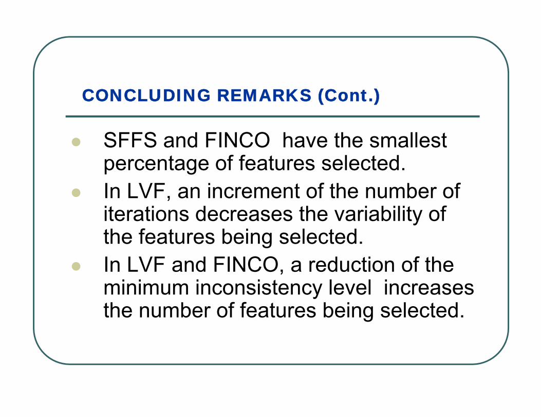
SFFS and FINCO have the smallest percentage of features selected.In LVF, an increment of the number of iterations decreases the variability of the features being selected. In LVF and FINCO, a reduction of the minimum inconsistency level increases the number of features being selected.

Data Reduction:Feature extraction-Principal components Analysis

Principal Components Analysis (PCA)The goal of Principal components analysis (Hotelling,1933) is to reduce the available information.

That is, the information contained in p featuresX=(X1,….,Xp) can be reduced to Z=(Z1,….Zq),with q<p y where the new features Zi’s , called thePrincipal components are uncorrelated.

The principal components of a random vector X are the elementsof an orthogonal linear transformation of X

From a geometric point of view, application of principalcomponents is equivalent to apply a rotation of the coordinatesaxis.

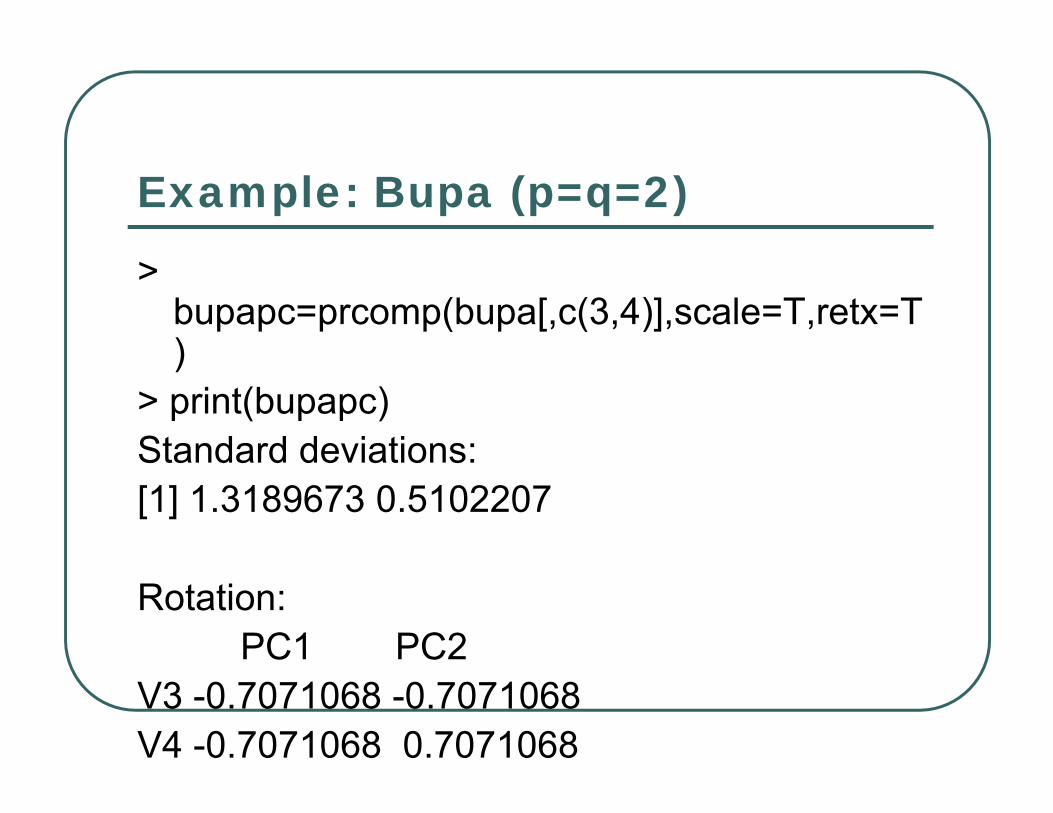
Example: Bupa (p=q=2)

> bupapc=prcomp(bupa[,c(3,4)],scale=T,retx=T)

> print(bupapc)Standard deviations:[1] 1.3189673 0.5102207

Rotation:PC1 PC2

V3 -0.7071068 -0.7071068V4 -0.7071068 0.7071068

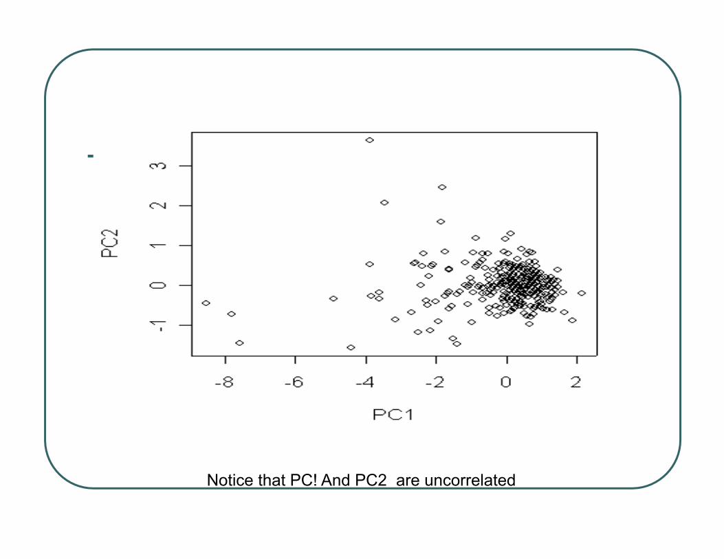
Notice that PC! And PC2 are uncorrelated

Finding the principal Components To determine the Principal components Z, we must find an

orthogonal matrix V such thati) Z=X*V ,

where X* is obtained by normalizing each column of X.and ii) Z’Z=(X*V)’(X*V) =V’X*’X*V

=diag(λ1,….,λp)It can be shown that VV’=V’V=I, and that the λj’s are the

eigenvalues of the correlation matrix X*’X*. V is found using singular value decomposition of X*’X*. The matrix V is called the loadings matrix and contains the

coefficients of all the features in each PC.

PCA AS AN OPTIMIZATION PROBLEM

X (nxp)T( nxp )

Matrix of components

Tk= argmax var ( Xγ )γ’γ=1

Subject to the orthogonality constrain

γj’ S γk = 0 ∀ 1≤ j < k

S

S=X’X, Covariance Matrix

From (ii) the j-th principal component Zj has standard deviation and it can be written as:

where vj1,vj2,…..vjp are the elements of the j-th column in V.

The calculated values of the principal component Zj are called the rotated values or simply the “scores”.

jλ

**22

*11 ..... ppjjjj XvXvXvZ +++=

Choice of the number of principal components

There are plenty of alternatives (Ferre, 1994), but the most used are:

i) Choose the number of components with an acumulative proportion of eigenvalues ( i.e, variance) of at least 75 percent.

ii) Choose up to the component whose eigenvalue is greater than 1. Use “Scree Plot”.

Example:Bupa> a=prcomp(bupa[,-7],scale=T)> print(a)Standard deviations:[1] 1.5819918 1.0355225 0.9854934 0.8268822 0.7187226 0.5034896

Rotation:PC1 PC2 PC3 PC4 PC5 PC6

V1 0.2660076 0.67908900 0.17178567 -0.6619343 0.01440487 0.014254815

V2 0.1523198 0.07160045 -0.97609467 -0.1180965 -0.03508447 0.061102720

V3 0.5092169 -0.38370076 0.12276631 -0.1487163 -0.29177970 0.686402469

V4 0.5352429 -0.29688378 0.03978484 -0.1013274 -0.30464653 -0.721606152

V5 0.4900701 -0.05236669 0.02183660 0.1675108 0.85354943 0.002380586

V6 0.3465300 0.54369383 0.02444679 0.6981780 -0.30343047 0.064759576

Example(cont)> summary(a)Importance of components:

PC1 PC2 PC3 PC4 PC5 PC6Standard deviation 1.582 1.036 0.985 0.827 0.7187 0.5035Proportion of Variance 0.417 0.179 0.162 0.114 0.0861 0.0423Cumulative Proportion 0.417 0.596 0.758 0.872 0.9577 1.0000>

Remarks

Several studies have shown that PCA does not give goods predictions in supervised classification.Better alternatives: Generalized PLS (Vega,2004) and Supervised PCA( Hastie, Tibshirani, 2004, Acuna and Porras, 2006).