comp 9517 computer vision - webcms3 comp 9517 s2 2010comp9517 s2 2016 13 chapter 3 image enhancement...

01/08/2016 COMP9517 S2 2016 1

COMP 9517 Computer Vision

Image Processing

01/08/2016 COMP9517 S2 2016 2

Image Analysis •  Manipulation of image data to extract the information

necessary for solving an imaging problem •  It is a data reduction process. •  Consists of preprocessing, data reduction and feature

analysis •  Preprocessing removes noise, eliminates irrelevant

information •  Data reduction extracts features for the analysis process •  During feature analysis, the extracted features are

examined and evaluated for their use in the application

01/08/2016 COMP9517 S2 2016 3

Image Preprocessing •  Input and output are intensity images

•  Aim to improve image, by suppressing distortions and enhancing image features, so that result is more suitable for a specific application

•  Exploit redundancy in image: for example, neighbouring pixels have similar brightness value.

•  Spatial and frequency domain techniques.

01/08/2016 COMP9517 S2 2016 4

4

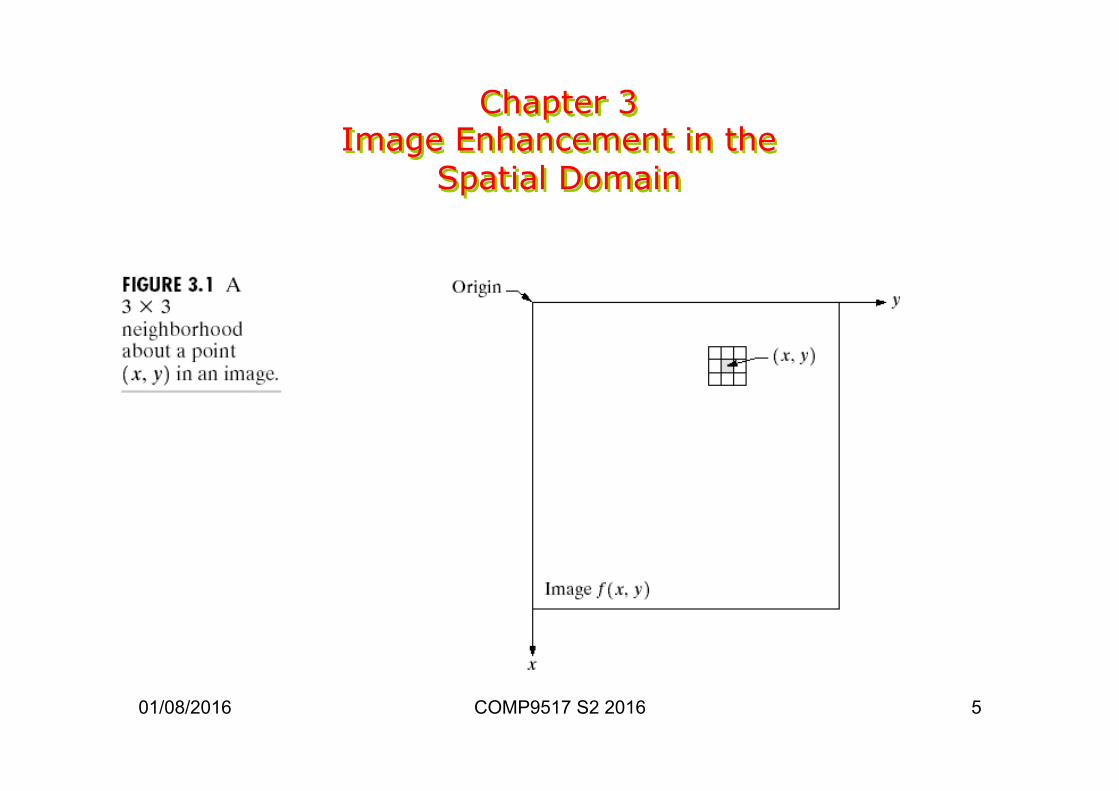
Spatial Domain Techniques •  Operate directly on image pixels: g (x, y) = T [ f(x, y) ] where

–  f (x,y) is the input image –  g(x, y) is the processed image –  T is an operator on f, over a nbd of (x, y), usually square or

rectangular nbd used. •  When T is of size 1 x 1, T becomes a gray-level

transformation function: s = T (r) •  Examples are contrast stretching, thresholding

01/08/2016 COMP9517 S2 2016 5

Chapter 3 Image Enhancement in the

Spatial Domain

01/08/2016 COMP9517 S2 2016 6


Spatial Domain

01/08/2016 COMP9517 S2 2016 7

Basic Gray level Transformations Image Negatives •  For input image with gray levels in range [0, L-1] , the negative

transformation is s = L - 1 - r

•  Produces equivalent of a photo negative •  Useful for enhancing white or gray detail in dark regions of image, when

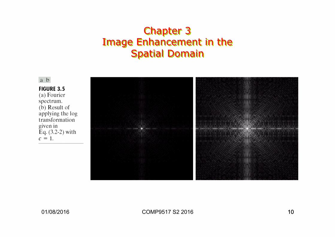
black areas are dominant Log Transformations s= c log (1 + r)

where c is constant, r >= 0 Maps narrow range of low gray-level values into wider range of output values

01/08/2016 COMP9517 S2 2016 8


Spatial Domain

01/08/2016 COMP9517 S2 2016 9


Spatial Domain

01/08/2016 COMP9517 S2 2016 10


Spatial Domain

10

01/08/2016 COMP9517 S2 2016 11

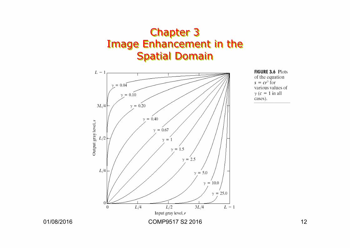
Power-Law Transformations •  Given by s = c rγ where c, γ are constant •  Similar to log transformation on input-output •  Family of possible transformations by varying γ •  Useful in displaying an image accurately on a

computer screen, for example on web sites!

01/08/2016 COMP9517 S2 2016 12


Spatial Domain

01/08/2016 COMP9517 S2 2016 COMP 9517 S2 2010 13


Spatial Domain

01/08/2016 COMP9517 S2 2016 COMP 9517 S2 2010 14


Spatial Domain

01/08/2016 COMP9517 S2 2016 15

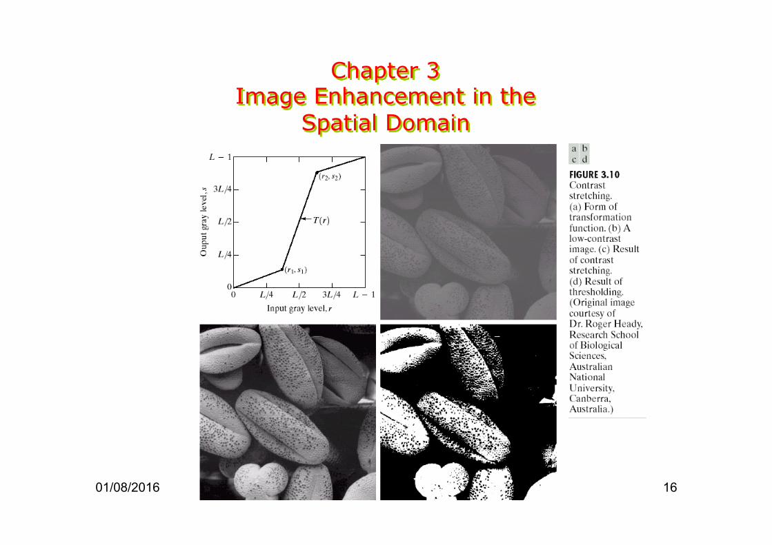
Piecewise-linear Transformations

Contrast Stretching •  To increase dynamic range of gray levels

in image.

01/08/2016 COMP9517 S2 2016 COMP 9517 S2 2010 16


Spatial Domain

01/08/2016 COMP9517 S2 2016 17

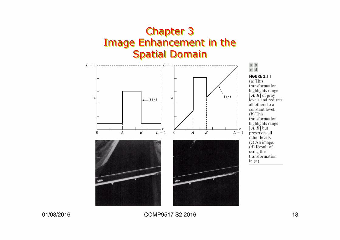
Gray-level Slicing •  Highlighting of specific range of gray levels

1. Display high value for all gray levels in range of interest, and low value for all others

2. Brighten the desired range of gray levels, preserve background and other gray-scale tones of image

01/08/2016 COMP9517 S2 2016 18


Spatial Domain

01/08/2016 COMP9517 S2 2016 19

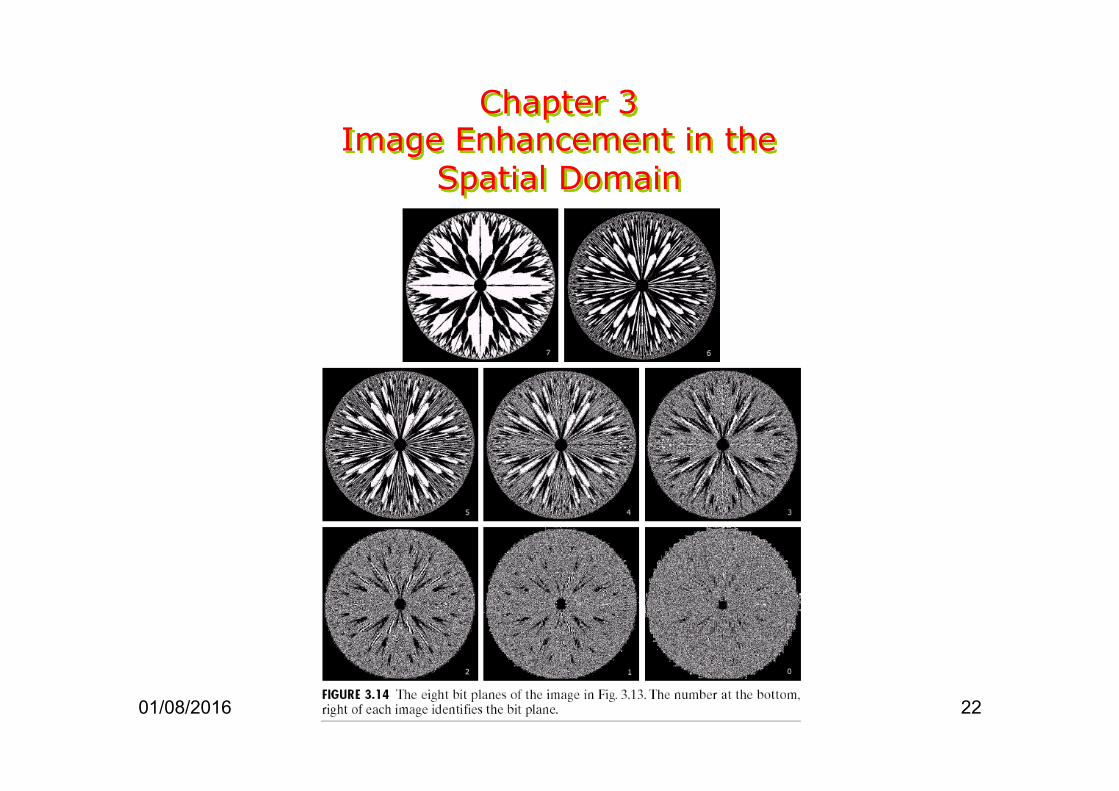
Bit-plane Slicing •  Highlights contribution made to total image

appearance by specific bits •  Eg, for an 8-bit image, there are 8 1-bit planes •  Useful in compression

01/08/2016 COMP9517 S2 2016 20


Spatial Domain

01/08/2016 COMP9517 S2 2016 21


Spatial Domain

01/08/2016 COMP9517 S2 2016 COMP 9517 S2 2010 22


Spatial Domain

01/08/2016 COMP9517 S2 2016 23

Histogram Processing

Histogram Equalization Aim: To get an image with equally

distributed brightness levels over the whole brightness scale.

01/08/2016 COMP9517 S2 2016 COMP 9517 S2 2010 24


Spatial Domain

01/08/2016 COMP9517 S2 2016 25

Histogram Processing (ctd)

Results: enhances contrast for brightness values near histogram maxima, decreases contrast near minima. Let r represent grey levels of the image. Let r be normalised in [0, 1], where r = 0 represents black r = 1 represents white

01/08/2016 COMP9517 S2 2016 COMP 9517 S2 2010 26


Spatial Domain

01/08/2016 COMP9517 S2 2016 27

Histogram equalization We consider transformations of the form s = T (r), 0 ≤ r ≤ 1 Also assume that T(r) satisfies:

a) T (r) is single-valued and monotonically increasing in 0 ≤ r ≤ 1 b) 0 ≤ T(r) ≤ 1 for 0 ≤ r ≤ 1 c)  guarantees that the inverse transformation exists, and monotonicity

preserves pixel order d)  guarantees that output grey levels will be in the same range as input

levels

01/08/2016 COMP9517 S2 2016 28

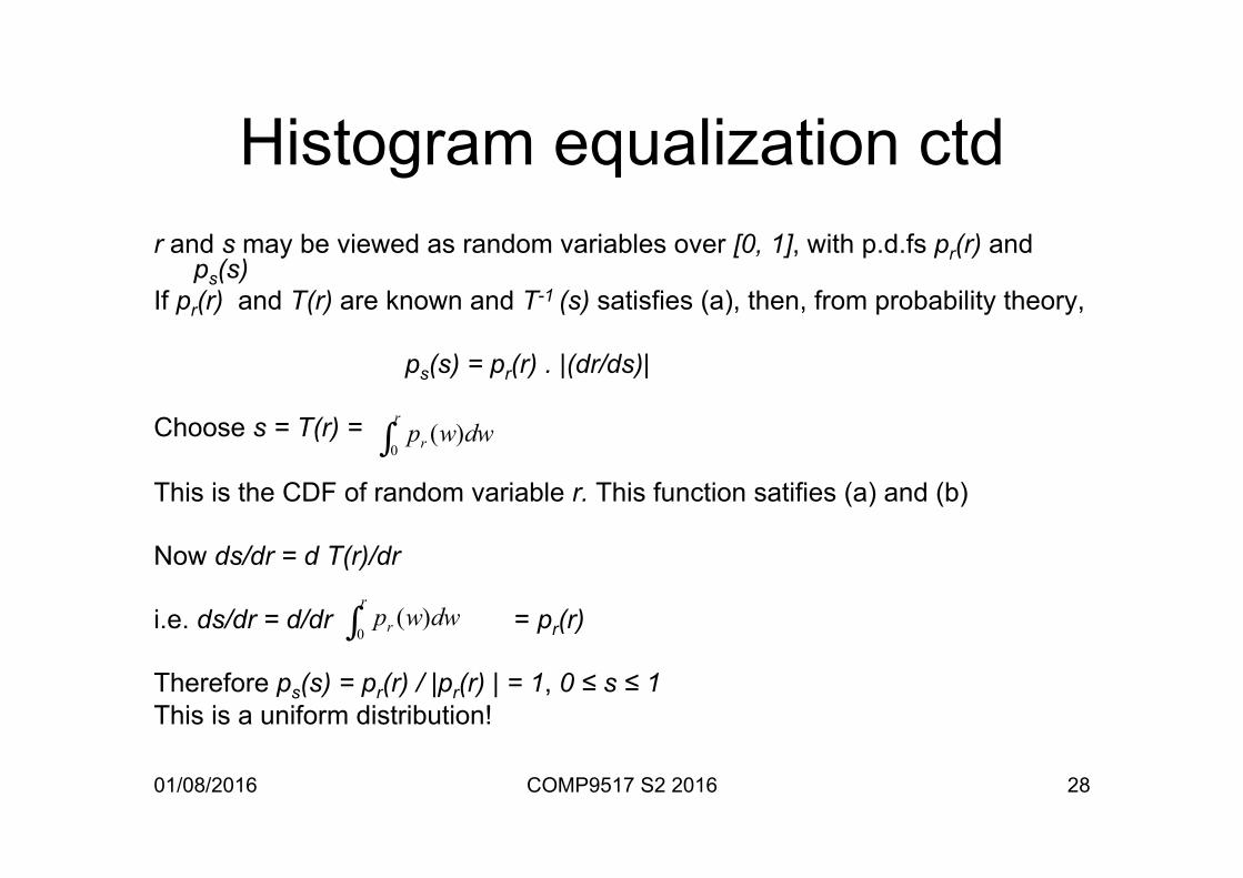
Histogram equalization ctd r and s may be viewed as random variables over [0, 1], with p.d.fs pr(r) and

ps(s) If pr(r) and T(r) are known and T-1 (s) satisfies (a), then, from probability theory,

ps(s) = pr(r) . |(dr/ds)|

Choose s = T(r) = This is the CDF of random variable r. This function satifies (a) and (b) Now ds/dr = d T(r)/dr i.e. ds/dr = d/dr = pr(r) Therefore ps(s) = pr(r) / |pr(r) | = 1, 0 ≤ s ≤ 1 This is a uniform distribution!

dwwpr

r )(0∫

dwwpr

r )(0∫

01/08/2016 COMP9517 S2 2016 29

Histogram equalization ctd For discrete values, we get probabilities and summations instead of p.d.fs and integrals: pr(rk) = nk / n , k = 0, 1,..., L-1 where n is total number of pixels in image, nk is number of pixels with gray level rk and L is total number of gray levels So sk = T (rk) = , k = 0, 1,..., L-1 This transformation is called histogram equalization

∑∑==

=k

j

jj

k

jr n

nrp

00)(

01/08/2016 COMP9517 S2 2016 COMP 9517 S2 2010 30


Spatial Domain

01/08/2016 COMP9517 S2 2016 31

Arithmetic/Logic Operations

•  On pixel-by-pixel basis between 2 or more images

•  AND and OR operations are used for masking- selecting subimages as RoI

•  Subtraction and addition are the most useful arithmetic operations

01/08/2016 COMP9517 S2 2016 32


Spatial Domain

01/08/2016 COMP9517 S2 2016 33


Spatial Domain

01/08/2016 COMP9517 S2 2016 34

Image Averaging •  Noisy image g (x, y) formed by adding noise n (x, y) to uncorrupted

image f (x, y): g (x, y) = f (x, y) + n (x, y) •  Assume that at each (x, y), the noise is uncorrelated and has zero

average value. •  Aim: To obtain smoothed result by adding a set of noisy images

gi (x, y), i = 1, 2, ..., K

g (x ,y)

•  As K increases, the variability of the pixel values decreases

•  Assumes that images are spatially registered

∑=

≈K

ii yxg

K 1

),(1

01/08/2016 COMP9517 S2 2016 COMP 9517 S2 2010 35


Spatial Domain

01/08/2016 COMP9517 S2 2016 36

Spatial Filtering •  These methods use a small neighbourhood of a pixel in the input

image to produce a new brightness value. •  Also called filtering techniques •  Neighbourhood of (x, y) is usually a square or rectangular subimage

centred at (x, y) •  A linear transformation calculates a value in the output image g (i, j)

as a linear combination of brightnesses in a local neighbourhood of the pixel in the input image f (i, j), weighted by coefficients h:

g (i, j) = •  This is a discrete convolution with a convolution mask h

∑∑ −− ),(),( nmfnjmih

01/08/2016 COMP9517 S2 2016 COMP 9517 S2 2010 37


Spatial Domain

01/08/2016 COMP9517 S2 2016 38


Spatial Domain

01/08/2016 COMP9517 S2 2016 39

Example Consider an image of constant intensity, with widely isolated pixels with different intensity from the background. We wish to detect these pixels. Use the following mask: -1 -1 -1 -1 8 -1 -1 -1 -1 Smoothing •  Aim: To suppress noise, other small fluctuations in image- may be

result of sampling, quantization, transmission, environment disturbances during acquisition

•  Uses redundancy in the image data •  May blur sharp edges, so care is needed

01/08/2016 COMP9517 S2 2016 40

Neighbourhood Averaging g (x, y) =

•  Replace intensity at pixel (x, y) with the average of the intensities in a neighbourhood of (x, y).

•  We can also use a weighted average, giving more importance to some pixels over others in the neighbourhood.

•  Neighbourhood averaging (also called mean filter) blurs edges.

∑∈Smn

mnfP ),(

),(1

01/08/2016 COMP9517 S2 2016 41


Spatial Domain

01/08/2016 COMP9517 S2 2016 COMP 9517 S2 2010 42


Spatial Domain

01/08/2016 COMP9517 S2 2016 43


Spatial Domain

01/08/2016 COMP9517 S2 2016 44

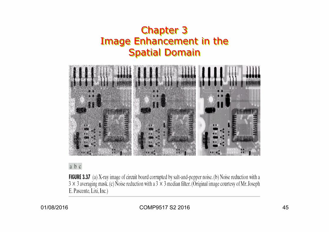
Order-Statistics Filters •  Nonlinear spatial filters- response based on ordering the pixels in

the neighbourhood, and replacing centre value with the ranking results.

Median Filter •  In median filtering, intensity of each pixel is replaced by the median •  of the intensities in a neighbourhood of the pixel •  Median M of a set of values is the middle value such that half the

values in the set are less than M and the other half greater than M •  Median filtering forces points with distinct intensities to be more like

their neighbours, thus eliminating isolated intensity spikes •  Good for impulse noise (salt-and-pepper noise) •  Other examples are max and min filters

01/08/2016 COMP9517 S2 2016 45


Spatial Domain

01/08/2016 COMP9517 S2 2016 46

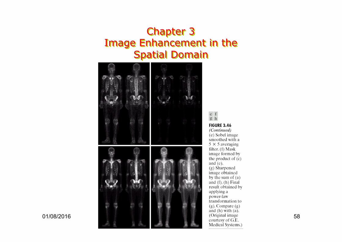
Sharpening Spatial Filters-Edge Detection

•  Goal is to highlight fine detail, or enhance detail that has been blurred

•  Spatial differentiation is the tool- strength of response of derivative operator is proportional to degree of discontinuity of the image at the point where operator is applied

•  Image differentiation enhances edges, and deemphasizes slowly varying gray-level values.

01/08/2016 COMP9517 S2 2016 COMP 9517 S2 2010 47


Spatial Domain

01/08/2016 COMP9517 S2 2016 48

Basic idea •  Horizontal scan of the image •  Edge modelled as a ramp- to represent blurring due to

sampling •  First derivative is 0 in regions of constant intensity,

constant during an intensity transition •  Second derivative is zero everywhere except at onset

and termination of intensity transition •  Thus, magnitude of first derivative can be used to detect

the presence of an edge, and sign of second derivative to determine whether a pixel lies on dark or light side of an edge.

01/08/2016 COMP9517 S2 2016 49

Gradient Operator Gx and Gy may be obtained by using masks- Sobel Operators. The magnitude of the gradient vector is G [ f(x, y) ] = This is commonly approximated by: G [ f(x, y) ] = | Gx | + | Gy | Now use numerical techniques to compute these Roberts’ 2x2 cross-gradient operators, Sobel’s 3x3 masks

22yx GG +

01/08/2016 COMP9517 S2 2016 50


Spatial Domain

50

01/08/2016 COMP9517 S2 2016 51

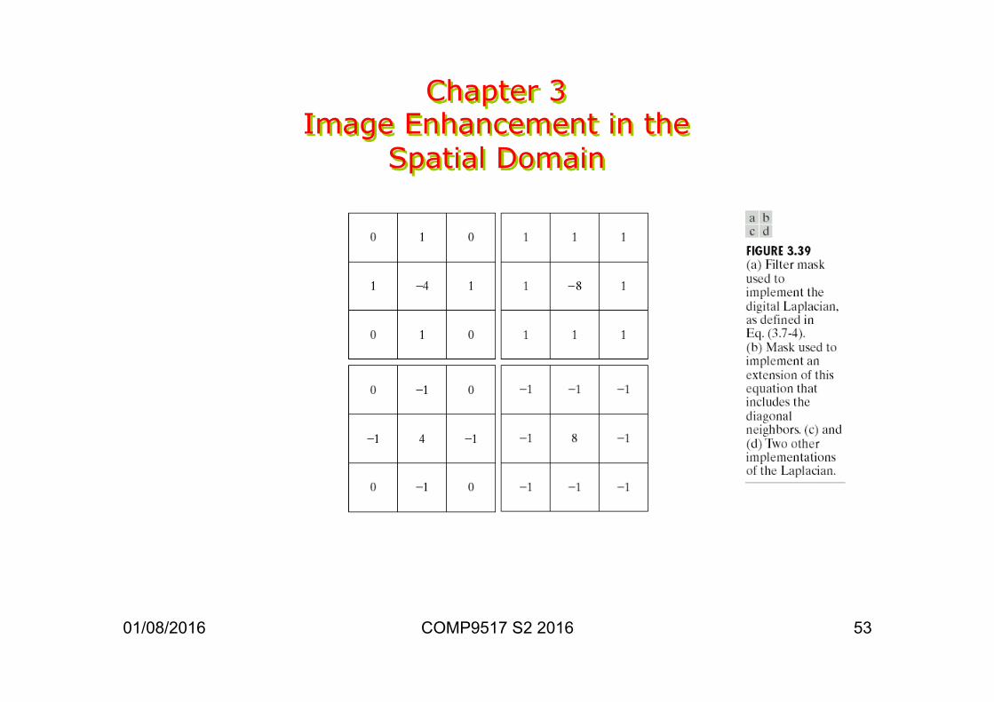
The Laplacian For a function f (x, y), the Laplacian is defined by This is a linear operator, as all derivative operators are. In discrete form: and similarly in y direction. Summing them gives us

2

2

2

22

yf

xff

∂

∂+

∂

∂=Δ

),(2),1(),1(2

2

yxfyxfyxfxf

−−++=∂

∂

),(4)]1,()1,(),1(),1([2 yxfyxfyxfyxfyxf −−+++−++=Δ

01/08/2016 COMP9517 S2 2016 52

Laplacian ctd •  There are other forms of the Laplacian- can include

diagonal directions, for example. •  Laplacian highlights grey-level discontinuities and

produces dark featureless backgrounds. •  The background can be recovered by adding or

subtracting the Laplacian image to the original image.

01/08/2016 COMP9517 S2 2016 53


Spatial Domain

01/08/2016 COMP9517 S2 2016 COMP 9517 S2 2010 54


Spatial Domain

01/08/2016 COMP9517 S2 2016 COMP 9517 S2 2010 55


Spatial Domain

01/08/2016 COMP9517 S2 2016 56


Spatial Domain

01/08/2016 COMP9517 S2 2016 COMP 9517 S2 2010 57


Spatial Domain

01/08/2016 COMP9517 S2 2016 COMP 9517 S2 2010 58


Spatial Domain

01/08/2016 COMP9517 S2 2016

References and Acknowledgements

•  Chapter 3, Gonzalez and Woods 2002 •  Szeliski 3.1-3.3 •  Images drawn from Gonzalez and Woods,

2002

59

comp 9517 computer vision - webcms3 comp 9517 s2 2010comp9517 s2 2016 13 chapter 3 image enhancement...

Documents