compactifications of margulis space-timesmathsci.kaist.ac.kr/~schoi/kyoto2015talkii.v2.pdf ·...
TRANSCRIPT
Compactifications of Margulis space-times
Suhyoung Choi
Department of Mathematical Science
KAIST, Daejeon, South Korea
mathsci.kaist.ac.kr/∼schoi
email: [email protected]
Geometry of Moduli Spaces of Low Dimensional Manifolds, RIMS, Kyoto,
December 14–18, 2015 (joint work with William Goldman, later part also Todd Drumm)
1/29

Abstract
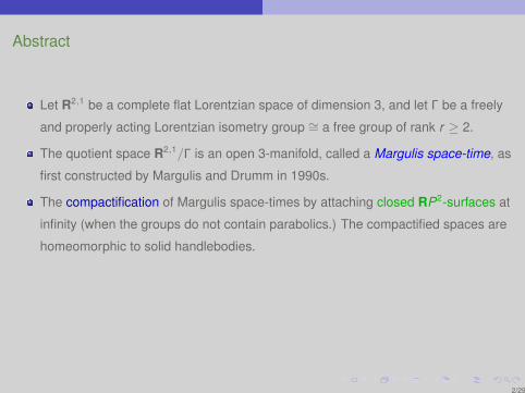
Let R2,1 be a complete flat Lorentzian space of dimension 3, and let Γ be a freely
and properly acting Lorentzian isometry group ∼= a free group of rank r ≥ 2.
The quotient space R2,1/Γ is an open 3-manifold, called a Margulis space-time, as
first constructed by Margulis and Drumm in 1990s.
The compactification of Margulis space-times by attaching closed RP2-surfaces at
infinity (when the groups do not contain parabolics.) The compactified spaces are
homeomorphic to solid handlebodies.
Finally, we will discuss about the parabolic regions of tame Margulis space-times
with parabolic holonomies.
There is another contemporary approach by Danciger, Gueritaud and Kassel.
2/29

Abstract
Let R2,1 be a complete flat Lorentzian space of dimension 3, and let Γ be a freely
and properly acting Lorentzian isometry group ∼= a free group of rank r ≥ 2.
The quotient space R2,1/Γ is an open 3-manifold, called a Margulis space-time, as
first constructed by Margulis and Drumm in 1990s.
The compactification of Margulis space-times by attaching closed RP2-surfaces at
infinity (when the groups do not contain parabolics.) The compactified spaces are
homeomorphic to solid handlebodies.
Finally, we will discuss about the parabolic regions of tame Margulis space-times
with parabolic holonomies.
There is another contemporary approach by Danciger, Gueritaud and Kassel.
2/29

Content
1 Main results
Background
2 Part I: Projective boosts
3 Part II: the bordifying surface
4 Part III. Γ acts properly on E ∪ Σ.
5 Part IV: the compactness
6 Part V: Margulis spacetime with parabolics
3/29

Main results Background
Background
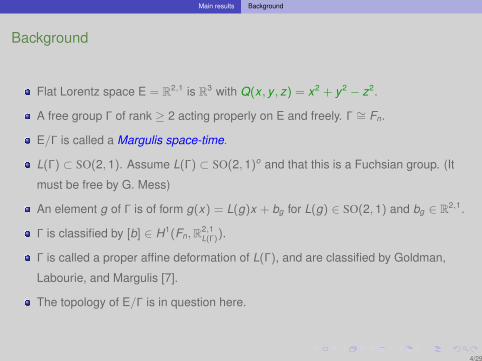
Flat Lorentz space E = R2,1 is R3 with Q(x , y , z) = x2 + y2 − z2.
A free group Γ of rank ≥ 2 acting properly on E and freely. Γ ∼= Fn.
E/Γ is called a Margulis space-time.
L(Γ) ⊂ SO(2, 1). Assume L(Γ) ⊂ SO(2, 1)o and that this is a Fuchsian group. (It
must be free by G. Mess)
An element g of Γ is of form g(x) = L(g)x + bg for L(g) ∈ SO(2, 1) and bg ∈ R2,1.
Γ is classified by [b] ∈ H1(Fn,R2,1L(Γ)).
Γ is called a proper affine deformation of L(Γ), and are classified by Goldman,
Labourie, and Margulis [7].
The topology of E/Γ is in question here.
4/29

Main results Background
Background
Flat Lorentz space E = R2,1 is R3 with Q(x , y , z) = x2 + y2 − z2.
A free group Γ of rank ≥ 2 acting properly on E and freely. Γ ∼= Fn.
E/Γ is called a Margulis space-time.
L(Γ) ⊂ SO(2, 1). Assume L(Γ) ⊂ SO(2, 1)o and that this is a Fuchsian group. (It
must be free by G. Mess)
An element g of Γ is of form g(x) = L(g)x + bg for L(g) ∈ SO(2, 1) and bg ∈ R2,1.
Γ is classified by [b] ∈ H1(Fn,R2,1L(Γ)).
Γ is called a proper affine deformation of L(Γ), and are classified by Goldman,
Labourie, and Margulis [7].
The topology of E/Γ is in question here.
4/29

Main results Background
The tameness
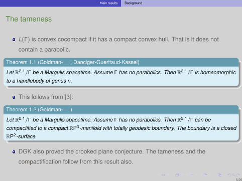
L(Γ) is convex cocompact if it has a compact convex hull. That is it does not
contain a parabolic.
Theorem 1.1 (Goldman- , Danciger-Gueritaud-Kassel)
Let R2,1/Γ be a Margulis spacetime. Assume Γ has no parabolics. Then R2,1/Γ is homeomorphic
to a handlebody of genus n.
This follows from [3]:
Theorem 1.2 (Goldman- )
Let R2,1/Γ be a Margulis spacetime. Assume Γ has no parabolics. Then R2,1/Γ can be
compactified to a compact RP3-manifold with totally geodesic boundary. The boundary is a closed
RP2-surface.
DGK also proved the crooked plane conjecture. The tameness and the
compactification follow from this result also.
5/29

Main results Background
The tameness
L(Γ) is convex cocompact if it has a compact convex hull. That is it does not
contain a parabolic.
Theorem 1.1 (Goldman- , Danciger-Gueritaud-Kassel)
Let R2,1/Γ be a Margulis spacetime. Assume Γ has no parabolics. Then R2,1/Γ is homeomorphic
to a handlebody of genus n.
This follows from [3]:
Theorem 1.2 (Goldman- )
Let R2,1/Γ be a Margulis spacetime. Assume Γ has no parabolics. Then R2,1/Γ can be
compactified to a compact RP3-manifold with totally geodesic boundary. The boundary is a closed
RP2-surface.
DGK also proved the crooked plane conjecture. The tameness and the
compactification follow from this result also.
5/29

Part I: Projective boosts
The real projective geometry
RPn = P(Rn+1) = Rn+1 − {O}/ ∼ where v ∼ w if v = sw for s 6= 0.
The real projective geometry is given by RPn with the standard
PGL(n + 1,R)-action.
The oriented version Sn := S(Rn+1) = Rn+1 − {O}/ ∼ where v ∼ w if v = sw for
s > 0.
The group Aut(Sn) of projective automorphisms ∼= SL±(n + 1,R).
The projection (x1, · · · , xn+1)→ (( x1, · · · , xn+1 )) , the equivalence class.
6/29

Part I: Projective boosts
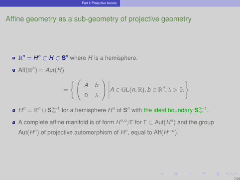
Affine geometry as a sub-geometry of projective geometry
Rn = Ho ⊂ H ⊂ Sn where H is a hemisphere.
Aff(Rn) = Aut(H)
=
{ A b
0 λ
∣∣∣∣∣A ∈ GL(n,R), b ∈ Rn, λ > 0.
}
Hn = Rn ∪ Sn−1∞ for a hemisphere Hn of Sn with the ideal boundary Sn−1
∞ .
A complete affine manifold is of form Hn,o/Γ for Γ ⊂ Aut(Hn) and the group
Aut(Hn) of projective automorphism of Hn, equal to Aff(Hn,o).
7/29
Part I: Projective boosts
Affine geometry as a sub-geometry of projective geometry
Rn = Ho ⊂ H ⊂ Sn where H is a hemisphere.
Aff(Rn) = Aut(H)
=
{ A b
0 λ
∣∣∣∣∣A ∈ GL(n,R), b ∈ Rn, λ > 0.
}
Hn = Rn ∪ Sn−1∞ for a hemisphere Hn of Sn with the ideal boundary Sn−1
∞ .
A complete affine manifold is of form Hn,o/Γ for Γ ⊂ Aut(Hn) and the group
Aut(Hn) of projective automorphism of Hn, equal to Aff(Hn,o).
7/29

Part I: Projective boosts
Lorentz geometry compactified
R2,1 = H o the interior of a 3-hemisphere H in S3.
Isom(R2,1) = R3 o SO(2, 1) ↪→ Aut(H ) ↪→ SL±(4,R).
H = R2,1 ∪ S2∞ is the compactification of R2,1 with the ideal boundary S2
∞.
A element of Isom(R2,1) with a semisimple linear part is a Lorentzian boost.
g
x1
x2
x3
=
el 0 0
0 1 0
0 0 e−l
x1
x2
x3
+
0
b
0
.
8/29

Part I: Projective boosts
Lorentzian boost
As an element of SL±(4,R),
γ =
el 0 0 0
0 1 0 α
0 0 e−l 0
0 0 0 1
, α 6= 0.
The six fixed points on S2∞ are:
x+± := (( ±1 : 0 : 0 : 0 )) , x0
± := (( 0 : ±1 : 0 : 0 )) , x−± := (( 0 : 0 : ±1 : 0 )) .
in homogeneous coordinates on S2∞.
Axis(γ) := x0Ox0−. γ acts as a translation on Axis(γ) towards x0
+ when α > 0 and
towards x0− when α < 0.
Define the weak stable plane W wu(γ) := span(x−(γ) ∪ Axis(γ)
).
9/29

Part I: Projective boosts
Projective boosts
A Lorentzian boost is any isometry g conjugate to γ.
A projective boost is a projective extension S3 of a Lorentzian boost.
The elements x±± (g), x0±(g) are all determined by g itself.
10/29

Part I: Projective boosts
Projective boosts
A Lorentzian boost is any isometry g conjugate to γ.
A projective boost is a projective extension S3 of a Lorentzian boost.
The elements x±± (g), x0±(g) are all determined by g itself.
10/29

Part I: Projective boosts
-1.0-0.5
0.0
0.5
1.0
-1.0-0.5
0.00.5
1.0-1.0
-0.5
0.0
0.5
1.0
e3
e3−
e2e2−
η+
η−
e1
e1−
x
y
z
Figure: The action of a projective boost g on the 3-hemisphere H with the boundary sphere S2∞.
11/29
Part I: Projective boosts
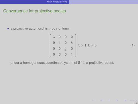
Convergence for projective boosts
a projective automorphism gλ,k of formλ 0 0 0
0 1 0 k
0 0 1λ
0
0 0 0 1
λ > 1, k 6= 0 (1)
under a homogeneous coordinate system of S3 is a projective-boost.
Assume (λ, k)→∞ and k/λ→ 0.
(a) gλ,k |H − S2∞ attracting fixed points e1, e1−.
(b) gλ,k |(S ∩H )− η− → e2 for the stable subspace S.
(c) K ⊂ H − η−, K meets both component of H − S. Then gλ,k (K )→ η+.
12/29

Part I: Projective boosts
Convergence for projective boosts
a projective automorphism gλ,k of formλ 0 0 0
0 1 0 k
0 0 1λ
0
0 0 0 1
λ > 1, k 6= 0 (1)
under a homogeneous coordinate system of S3 is a projective-boost.
Assume (λ, k)→∞ and k/λ→ 0.
(a) gλ,k |H − S2∞ attracting fixed points e1, e1−.
(b) gλ,k |(S ∩H )− η− → e2 for the stable subspace S.
(c) K ⊂ H − η−, K meets both component of H − S. Then gλ,k (K )→ η+.
12/29

Part II: the bordifying surface
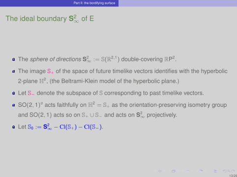
The ideal boundary S2∞ of E
The sphere of directions S2∞ := S(R2,1) double-covering RP2.
The image S+ of the space of future timelike vectors identifies with the hyperbolic
2-plane H2, (the Beltrami-Klein model of the hyperbolic plane.)
Let S− denote the subspace of S corresponding to past timelike vectors.
SO(2, 1)o acts faithfully on H2 = S+ as the orientation-preserving isometry group
and SO(2, 1) acts so on S+ ∪ S− and acts on S2∞ projectively.
Let S0 := S2∞ − Cl(S+)− Cl(S−).
13/29
Part II: the bordifying surface
Oriented Lorentzian space E
R2,1 × R2,1 → R, (v , u) 7→ v · u.
R2,1 × R2,1 × R2,1 → R, (v , u,w) 7→ Det(v , u,w).
Null space N := {v |v · v = 0} ⊂ R2,1.
Let v ∈ N , v 6= 0, v⊥ − Rv has two choices of components.
Define the null half-plane W (v) (or the wing) associated to v as:
W (v) :={
w ∈ v⊥ | Det(v,w, u) > 0}⊂ v⊥ − Rv.
where u is chosen arbitrarily in the same Cl(S±) that v is in.
W (v) = W (−v).
14/29

Part II: the bordifying surface
The corresponding set of directions is the open arc
ε(
(( v )))
:= (( W (v) ))
in S0 joining (( v )) to its antipode (( v− )) .
The corresponding map
(( v )) 7−→ ε(
(( v )))
is an SO(2, 1)-equivariant map
∂S+ → S
where S denotes the set of half-arcs.
15/29
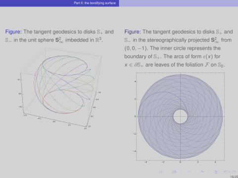
Part II: the bordifying surface
Figure: The tangent geodesics to disks S+ and
S− in the unit sphere S2∞ imbedded in R3.
-1.0
-0.5
0.0
0.5
1.0
-1.0
-0.5
0.0
0.5
1.0
-0.5
0.0
0.5
Figure: The tangent geodesics to disks S+ and
S− in the stereographically projected S2∞ from
(0, 0,−1). The inner circle represents the
boundary of S+. The arcs of form ε(x) for
x ∈ ∂S+ are leaves of the foliation F on S0.
-4 -2 0 2 4
-4
-2
0
2
4
16/29

Part II: the bordifying surface
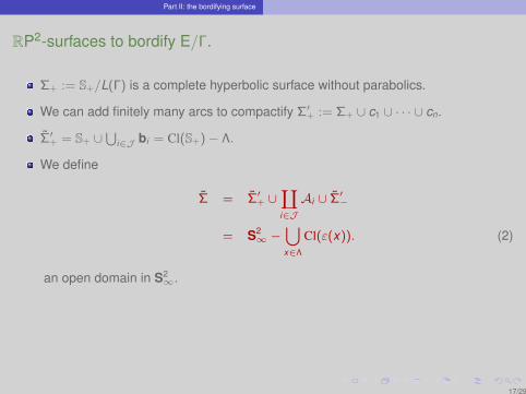
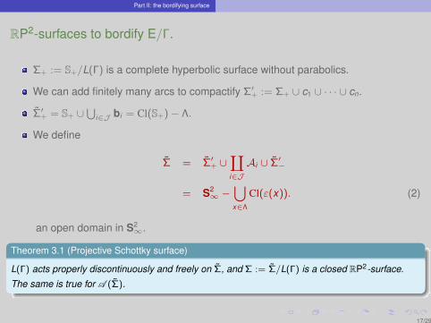
RP2-surfaces to bordify E/Γ.
Σ+ := S+/L(Γ) is a complete hyperbolic surface without parabolics.
We can add finitely many arcs to compactify Σ′+ := Σ+ ∪ c1 ∪ · · · ∪ cn.
Σ′+ = S+ ∪⋃
i∈J bi = Cl(S+)− Λ.
We define
Σ = Σ′+ ∪∐i∈J
Ai ∪ Σ′−
= S2∞ −
⋃x∈Λ
Cl(ε(x)). (2)
an open domain in S2∞.
Theorem 3.1 (Projective Schottky surface)
L(Γ) acts properly discontinuously and freely on Σ, and Σ := Σ/L(Γ) is a closed RP2-surface.
The same is true for A (Σ).
17/29
Part II: the bordifying surface
RP2-surfaces to bordify E/Γ.
Σ+ := S+/L(Γ) is a complete hyperbolic surface without parabolics.
We can add finitely many arcs to compactify Σ′+ := Σ+ ∪ c1 ∪ · · · ∪ cn.
Σ′+ = S+ ∪⋃
i∈J bi = Cl(S+)− Λ.
We define
Σ = Σ′+ ∪∐i∈J
Ai ∪ Σ′−
= S2∞ −
⋃x∈Λ
Cl(ε(x)). (2)
an open domain in S2∞.
Theorem 3.1 (Projective Schottky surface)
L(Γ) acts properly discontinuously and freely on Σ, and Σ := Σ/L(Γ) is a closed RP2-surface.
The same is true for A (Σ).
17/29
Part III. Γ acts properly on E ∪ Σ.
The proper action of Γ on E ∪ Σ
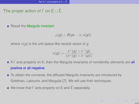
Recall the Margulis invariant:
µ(g) = B(gx − x , v(g))
where v(g) is the unit space-like neutral vector of g
v(g) :=x+(g)× x−(g)
||x+(g)× x−(g)|| .
If Γ acts properly on E, then the Margulis invariants of nonidentity elements are all
positive or all negative.
To obtain the converse, the diffused Margulis invariants are introduced by
Goldman, Labourie, and Margulis [7]. We will use their techniques.
We know that Γ acts properly on E and Σ separately.
18/29

Part III. Γ acts properly on E ∪ Σ.
The proper action of Γ on E ∪ Σ
Recall the Margulis invariant:
µ(g) = B(gx − x , v(g))
where v(g) is the unit space-like neutral vector of g
v(g) :=x+(g)× x−(g)
||x+(g)× x−(g)|| .
If Γ acts properly on E, then the Margulis invariants of nonidentity elements are all
positive or all negative.
To obtain the converse, the diffused Margulis invariants are introduced by
Goldman, Labourie, and Margulis [7]. We will use their techniques.
We know that Γ acts properly on E and Σ separately.
18/29

Part III. Γ acts properly on E ∪ Σ.
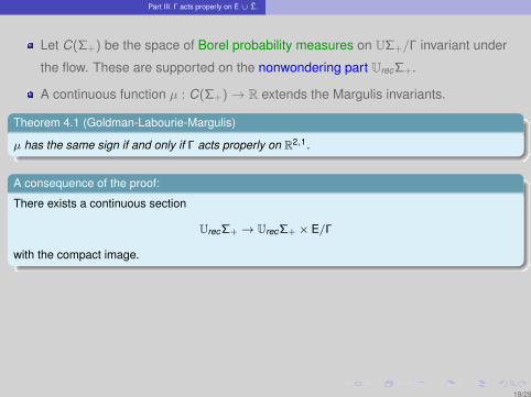
Let C(Σ+) be the space of Borel probability measures on UΣ+/Γ invariant under
the flow. These are supported on the nonwondering part UrecΣ+.
A continuous function µ : C(Σ+)→ R extends the Margulis invariants.
Theorem 4.1 (Goldman-Labourie-Margulis)
µ has the same sign if and only if Γ acts properly on R2,1.
A consequence of the proof:
There exists a continuous section
UrecΣ+ → UrecΣ+ × E/Γ
with the compact image.
Goldman-Labourie found a one to one correspondence
{l|l is a nonwandering geodesic on Σ+} ↔ {l|l is a nonwandering spacelike geodesic on E/Γ}
A key fact: Closed geodesics on Σ+ corresponds to closed geodesic in E/Γ. The
set is precompact
19/29
Part III. Γ acts properly on E ∪ Σ.
Let C(Σ+) be the space of Borel probability measures on UΣ+/Γ invariant under
the flow. These are supported on the nonwondering part UrecΣ+.
A continuous function µ : C(Σ+)→ R extends the Margulis invariants.
Theorem 4.1 (Goldman-Labourie-Margulis)
µ has the same sign if and only if Γ acts properly on R2,1.
A consequence of the proof:
There exists a continuous section
UrecΣ+ → UrecΣ+ × E/Γ
with the compact image.
Goldman-Labourie found a one to one correspondence
{l|l is a nonwandering geodesic on Σ+} ↔ {l|l is a nonwandering spacelike geodesic on E/Γ}
A key fact: Closed geodesics on Σ+ corresponds to closed geodesic in E/Γ. The
set is precompact
19/29

Part III. Γ acts properly on E ∪ Σ.
The proof of the properness
Let K be a compact subset of E ∪ Σ.
Consider {g ∈ Γ|g(K ) ∩ K 6= ∅}.
Suppose that the set is not finite. We find a sequence gi with λ(gi )→∞.
Let ai and ri on ∂S+ denote the attracting and the repelling fixed points of gi .
Since a Fuchsian group is a convergence group: There exists a subsequence gi
so that
ai → a, bi → b, a, b ∈ ∂S+, λi →∞.
Assume a 6= b. The other case will be done by “Margulis trick”
20/29

Part III. Γ acts properly on E ∪ Σ.
-1.0-0.5
0.0
0.5
1.0
-1.0-0.5
0.00.5
1.0-1.0
-0.5
0.0
0.5
1.0
e3
e3−
e2e2−
η+
η−
e1
e1−
x
y
z
Figure: The actions are very close to this one.
21/29

Part III. Γ acts properly on E ∪ Σ.
By the boundedness of nonwandering spacelike geodesics in E/Γ, we find a
bounded set hi ∈ SL±(4,R) so that higih−1i is in the standard form.
We choose a subsequence hi → h∞ ∈ SL±(4,R) and the stable subspace
Si → S∞.
Cover K by a finite set of convex ball meeting S∞ and ones disjoint from S∞.
gi (B)→ a, a− for disjoint balls.
gi (B′)→ ε(a) for B′ meeting S∞.
22/29

Part IV: the compactness
Compactness
Now we know E ∩ Σ/Γ is a manifold.
We know Σ is a closed surface. π1(Σ)→ π1(M) surjective.
23/29

Part V: Margulis spacetime with parabolics
Margulis spacetime with parabolics
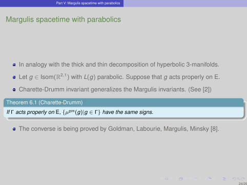
In analogy with the thick and thin decomposition of hyperbolic 3-manifolds.
Let g ∈ Isom(R2,1) with L(g) parabolic. Suppose that g acts properly on E.
Charette-Drumm invariant generalizes the Margulis invariants. (See [2])
Theorem 6.1 (Charette-Drumm)
If Γ acts properly on E, {µgen(g)|g ∈ Γ} have the same signs.
The converse is being proved by Goldman, Labourie, Margulis, Minsky [8].
24/29
Part V: Margulis spacetime with parabolics
Margulis spacetime with parabolics
In analogy with the thick and thin decomposition of hyperbolic 3-manifolds.
Let g ∈ Isom(R2,1) with L(g) parabolic. Suppose that g acts properly on E.
Charette-Drumm invariant generalizes the Margulis invariants. (See [2])
Theorem 6.1 (Charette-Drumm)
If Γ acts properly on E, {µgen(g)|g ∈ Γ} have the same signs.
The converse is being proved by Goldman, Labourie, Margulis, Minsky [8].
24/29

Part V: Margulis spacetime with parabolics
Understanding the parabolic transformation
We restrict to the cyclic 〈g〉 for parabolic g.
U = exp(N) = I + N + 12 N2 where N is skew-adjoint nilpotent.
N = log(U) = (U − I) + 12 (U − I)2.
Lemma 6.2 (Skew-Nilpotent)
There exists c ∈ KerN such that c is causal, c = N(b), b ∈ R2,1 is space-like and b.b = 1.
Using basis {a, b, c} with b = N(a), c = N(b), we obtain a one-parameter family
containing U
Φ(t) : E→ E =
1 t t2/2 µt3/6
0 1 t µt2/2
0 0 1 µt
0 0 0 1
.
25/29

Part V: Margulis spacetime with parabolics
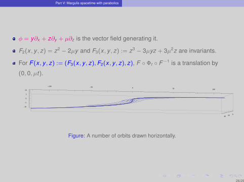
φ = y∂x + z∂y + µ∂z is the vector field generating it.
F2(x , y , z) = z2 − 2µy and F3(x , y , z) := z3 − 3µyz + 3µ2z are invariants.
For F (x , y , z) := (F3(x , y , z),F2(x , y , z), z), F ◦ Φt ◦ F−1 is a translation by
(0, 0, µt).
-100-50
050
100
020
40
-10
-5
0
5
10
Figure: A number of orbits drawn horizontally.
26/29
Part V: Margulis spacetime with parabolics
Lorentzian analog of parabolic neighborhoods
We use timelike ruled surface invariant under Φt .
F2 = T is a parabolic cylinder PT .
Take a line l with direction (a, 0, c), a, c > 0 in the timelike direction 2ac > 0.
Ψ(t , s) = Φt (l(s)) for l(s) = (0, y0, 0) + s(a, 0, c) for (0, y0, 0) ∈ PT where
T = −2µy0.
For y0 < µ ac , Ψ(t , s) is a proper imbedding to Φt invariant ruled surface.
Figure: The ruled surface
27/29

Part V: Margulis spacetime with parabolics
Lorentzian analog of parabolic neighborhoods
We use timelike ruled surface invariant under Φt .
F2 = T is a parabolic cylinder PT .
Take a line l with direction (a, 0, c), a, c > 0 in the timelike direction 2ac > 0.
Ψ(t , s) = Φt (l(s)) for l(s) = (0, y0, 0) + s(a, 0, c) for (0, y0, 0) ∈ PT where
T = −2µy0.
For y0 < µ ac , Ψ(t , s) is a proper imbedding to Φt invariant ruled surface.
Figure: The ruled surface27/29
References
References I
M. Berger, M. Cole, Geometry I, II, Springer Verlag.
V. Charette and T. Drumm,
Strong marked isospectrality of affine Lorentzian groups,
J. Differential Geom. 66 (2004), 437–452.
S. Choi and W. Goldman,
Topological tameness of Margulis spacetimes,
arXiv:1204.5308
D. Fried and W. Goldman,
Three-dimensional affine crystallographic groups,
Adv. in Math. 47 (1983), no. 1, 1–49.
D. Fried, W. Goldman, and M. Hirsch,
Affine manifolds with nilpotent holonomy,
Comment. Math. Helv. 56 (1981), 487–523.
W. Goldman and F. Labourie,
Geodesics in Margulis spacetimes,
Ergod. Theory Dynam. Systems 32 (2012), 643–651.
W. Goldman, F. Labourie, and G. Margulis,
Proper affine actions and geodesic flows of hyperbolic surfaces,
Ann. of Math. (2) 170 (2009), 1051–1083.
28/29

References
References II
W. Goldman, F. Labourie, G. Margulis, and Y. Minsky,
Complete flat Lorentz 3-manifolds and laminations on hyperbolic surfaces,
preprint, May 29, 2012
T. Tucker,
Non-compact 3-manifolds and the missing-boundary problem,
Topology 13 (1974), 267–273.
29/29