companies. a curr ent list of ibm trademarks is available ... · curr ent_time ... cast ..... . 46...

IBM Cognos AnalyticsVersion 11.0

Data Modeling Guide

IBM

©

Product Information

This document applies to IBM Cognos Analytics version 11.0.0 and may also apply to subsequent releases.

Copyright

Licensed Materials - Property of IBM

© Copyright IBM Corp. 2015, 2017.

US Government Users Restricted Rights – Use, duplication or disclosure restricted by GSA ADP Schedule Contractwith IBM Corp.

IBM, the IBM logo and ibm.com are trademarks or registered trademarks of International Business Machines Corp.,registered in many jurisdictions worldwide. Other product and service names might be trademarks of IBM or othercompanies. A current list of IBM trademarks is available on the Web at “Copyright and trademark information” atwww.ibm.com/legal/copytrade.shtml.

© Copyright IBM Corporation 2015, 2016.US Government Users Restricted Rights – Use, duplication or disclosure restricted by GSA ADP Schedule Contractwith IBM Corp.

http://www.ibm.com/legal/copytrade.shtml

Contents

Chapter 1. Data modeling in Cognos Analytics . . . . . . . . . . . . . . . . . . . 1

Chapter 2. Creating a data module . . . . . . . . . . . . . . . . . . . . . . . . 3Using a data module source . . . . . . . . . . . . . . . . . . . . . . . . . . . . . . 3Using a data server source. . . . . . . . . . . . . . . . . . . . . . . . . . . . . . . 4Using an uploaded file source . . . . . . . . . . . . . . . . . . . . . . . . . . . . . 4Using a data set source . . . . . . . . . . . . . . . . . . . . . . . . . . . . . . . . 5Using a package source . . . . . . . . . . . . . . . . . . . . . . . . . . . . . . . . 5

Chapter 3. Creating a simple data module . . . . . . . . . . . . . . . . . . . . . 7

Chapter 4. Refining a data module . . . . . . . . . . . . . . . . . . . . . . . . 9Relationships . . . . . . . . . . . . . . . . . . . . . . . . . . . . . . . . . . . 11

Creating a relationship from scratch . . . . . . . . . . . . . . . . . . . . . . . . . . 12Calculations . . . . . . . . . . . . . . . . . . . . . . . . . . . . . . . . . . . 13

Creating basic calculations . . . . . . . . . . . . . . . . . . . . . . . . . . . . . 13Grouping data . . . . . . . . . . . . . . . . . . . . . . . . . . . . . . . . . 14Cleaning data . . . . . . . . . . . . . . . . . . . . . . . . . . . . . . . . . 15Creating custom calculations . . . . . . . . . . . . . . . . . . . . . . . . . . . . 16

Creating navigation groups . . . . . . . . . . . . . . . . . . . . . . . . . . . . . . 17Filtering data . . . . . . . . . . . . . . . . . . . . . . . . . . . . . . . . . . . 18Hiding tables and columns . . . . . . . . . . . . . . . . . . . . . . . . . . . . . . 19Validating data modules . . . . . . . . . . . . . . . . . . . . . . . . . . . . . . . 20

Appendix A. Using the expression editor . . . . . . . . . . . . . . . . . . . . . 23Operators . . . . . . . . . . . . . . . . . . . . . . . . . . . . . . . . . . . . 23

( . . . . . . . . . . . . . . . . . . . . . . . . . . . . . . . . . . . . . . 23) . . . . . . . . . . . . . . . . . . . . . . . . . . . . . . . . . . . . . . 23* . . . . . . . . . . . . . . . . . . . . . . . . . . . . . . . . . . . . . . 23/ . . . . . . . . . . . . . . . . . . . . . . . . . . . . . . . . . . . . . . 23|| . . . . . . . . . . . . . . . . . . . . . . . . . . . . . . . . . . . . . 23+ . . . . . . . . . . . . . . . . . . . . . . . . . . . . . . . . . . . . . . 23- . . . . . . . . . . . . . . . . . . . . . . . . . . . . . . . . . . . . . . 24< . . . . . . . . . . . . . . . . . . . . . . . . . . . . . . . . . . . . . . 24<= . . . . . . . . . . . . . . . . . . . . . . . . . . . . . . . . . . . . . 24<> . . . . . . . . . . . . . . . . . . . . . . . . . . . . . . . . . . . . . 24= . . . . . . . . . . . . . . . . . . . . . . . . . . . . . . . . . . . . . . 24> . . . . . . . . . . . . . . . . . . . . . . . . . . . . . . . . . . . . . . 24>= . . . . . . . . . . . . . . . . . . . . . . . . . . . . . . . . . . . . . 24and . . . . . . . . . . . . . . . . . . . . . . . . . . . . . . . . . . . . . 25between . . . . . . . . . . . . . . . . . . . . . . . . . . . . . . . . . . . 25case . . . . . . . . . . . . . . . . . . . . . . . . . . . . . . . . . . . . . 25contains . . . . . . . . . . . . . . . . . . . . . . . . . . . . . . . . . . . 25distinct . . . . . . . . . . . . . . . . . . . . . . . . . . . . . . . . . . . . 25else . . . . . . . . . . . . . . . . . . . . . . . . . . . . . . . . . . . . . 26end . . . . . . . . . . . . . . . . . . . . . . . . . . . . . . . . . . . . . 26ends with . . . . . . . . . . . . . . . . . . . . . . . . . . . . . . . . . . . 26if . . . . . . . . . . . . . . . . . . . . . . . . . . . . . . . . . . . . . . 26in. . . . . . . . . . . . . . . . . . . . . . . . . . . . . . . . . . . . . . 26is missing . . . . . . . . . . . . . . . . . . . . . . . . . . . . . . . . . . . 26like . . . . . . . . . . . . . . . . . . . . . . . . . . . . . . . . . . . . . 26lookup . . . . . . . . . . . . . . . . . . . . . . . . . . . . . . . . . . . . 27not . . . . . . . . . . . . . . . . . . . . . . . . . . . . . . . . . . . . . 27or . . . . . . . . . . . . . . . . . . . . . . . . . . . . . . . . . . . . . 27

© Copyright IBM Corp. 2015, 2016 iii

starts with . . . . . . . . . . . . . . . . . . . . . . . . . . . . . . . . . . . 27then . . . . . . . . . . . . . . . . . . . . . . . . . . . . . . . . . . . . . 27when . . . . . . . . . . . . . . . . . . . . . . . . . . . . . . . . . . . . 28

Summaries . . . . . . . . . . . . . . . . . . . . . . . . . . . . . . . . . . . 28Statistical functions . . . . . . . . . . . . . . . . . . . . . . . . . . . . . . . . 28average. . . . . . . . . . . . . . . . . . . . . . . . . . . . . . . . . . . . 28count . . . . . . . . . . . . . . . . . . . . . . . . . . . . . . . . . . . . 29maximum . . . . . . . . . . . . . . . . . . . . . . . . . . . . . . . . . . . 29median . . . . . . . . . . . . . . . . . . . . . . . . . . . . . . . . . . . . 29minimum . . . . . . . . . . . . . . . . . . . . . . . . . . . . . . . . . . . 30percentage. . . . . . . . . . . . . . . . . . . . . . . . . . . . . . . . . . . 30percentile . . . . . . . . . . . . . . . . . . . . . . . . . . . . . . . . . . . 30quantile . . . . . . . . . . . . . . . . . . . . . . . . . . . . . . . . . . . 31quartile . . . . . . . . . . . . . . . . . . . . . . . . . . . . . . . . . . . . 32rank . . . . . . . . . . . . . . . . . . . . . . . . . . . . . . . . . . . . . 32tertile . . . . . . . . . . . . . . . . . . . . . . . . . . . . . . . . . . . . 33total . . . . . . . . . . . . . . . . . . . . . . . . . . . . . . . . . . . . . 33

Business Date/Time Functions . . . . . . . . . . . . . . . . . . . . . . . . . . . . . 34_add_seconds. . . . . . . . . . . . . . . . . . . . . . . . . . . . . . . . . . 34_add_minutes . . . . . . . . . . . . . . . . . . . . . . . . . . . . . . . . . 34_add_hours . . . . . . . . . . . . . . . . . . . . . . . . . . . . . . . . . . 35_add_days. . . . . . . . . . . . . . . . . . . . . . . . . . . . . . . . . . . 35_add_months . . . . . . . . . . . . . . . . . . . . . . . . . . . . . . . . . . 36_add_years . . . . . . . . . . . . . . . . . . . . . . . . . . . . . . . . . . 37_age . . . . . . . . . . . . . . . . . . . . . . . . . . . . . . . . . . . . . 37current_date . . . . . . . . . . . . . . . . . . . . . . . . . . . . . . . . . . 38current_time . . . . . . . . . . . . . . . . . . . . . . . . . . . . . . . . . . 38current_timestamp . . . . . . . . . . . . . . . . . . . . . . . . . . . . . . . . 38_day_of_week . . . . . . . . . . . . . . . . . . . . . . . . . . . . . . . . . 39_day_of_year . . . . . . . . . . . . . . . . . . . . . . . . . . . . . . . . . . 39_days_between . . . . . . . . . . . . . . . . . . . . . . . . . . . . . . . . . 39_days_to_end_of_month . . . . . . . . . . . . . . . . . . . . . . . . . . . . . . 39_end_of_day . . . . . . . . . . . . . . . . . . . . . . . . . . . . . . . . . . 40_first_of_month . . . . . . . . . . . . . . . . . . . . . . . . . . . . . . . . . 40_from_unixtime . . . . . . . . . . . . . . . . . . . . . . . . . . . . . . . . . 40_hour . . . . . . . . . . . . . . . . . . . . . . . . . . . . . . . . . . . . 41_last_of_month . . . . . . . . . . . . . . . . . . . . . . . . . . . . . . . . . 41_make_timestamp . . . . . . . . . . . . . . . . . . . . . . . . . . . . . . . . 41_minute . . . . . . . . . . . . . . . . . . . . . . . . . . . . . . . . . . . 41_month . . . . . . . . . . . . . . . . . . . . . . . . . . . . . . . . . . . . 42_months_between . . . . . . . . . . . . . . . . . . . . . . . . . . . . . . . . 42_second . . . . . . . . . . . . . . . . . . . . . . . . . . . . . . . . . . . 42_shift_timezone . . . . . . . . . . . . . . . . . . . . . . . . . . . . . . . . . 42_start_of_day . . . . . . . . . . . . . . . . . . . . . . . . . . . . . . . . . . 44_week_of_year . . . . . . . . . . . . . . . . . . . . . . . . . . . . . . . . . 44_timezone_hour . . . . . . . . . . . . . . . . . . . . . . . . . . . . . . . . . 44_timezone_minute . . . . . . . . . . . . . . . . . . . . . . . . . . . . . . . . 45_unix_timestamp . . . . . . . . . . . . . . . . . . . . . . . . . . . . . . . . 45_year . . . . . . . . . . . . . . . . . . . . . . . . . . . . . . . . . . . . 45_years_between . . . . . . . . . . . . . . . . . . . . . . . . . . . . . . . . . 45_ymdint_between . . . . . . . . . . . . . . . . . . . . . . . . . . . . . . . . 46

Common Functions. . . . . . . . . . . . . . . . . . . . . . . . . . . . . . . . . 46abs . . . . . . . . . . . . . . . . . . . . . . . . . . . . . . . . . . . . . 46cast . . . . . . . . . . . . . . . . . . . . . . . . . . . . . . . . . . . . . 46ceiling . . . . . . . . . . . . . . . . . . . . . . . . . . . . . . . . . . . . 47char_length . . . . . . . . . . . . . . . . . . . . . . . . . . . . . . . . . . 47coalesce . . . . . . . . . . . . . . . . . . . . . . . . . . . . . . . . . . . 48exp . . . . . . . . . . . . . . . . . . . . . . . . . . . . . . . . . . . . . 48floor . . . . . . . . . . . . . . . . . . . . . . . . . . . . . . . . . . . . . 48ln. . . . . . . . . . . . . . . . . . . . . . . . . . . . . . . . . . . . . . 49lower . . . . . . . . . . . . . . . . . . . . . . . . . . . . . . . . . . . . 49

iv IBM Cognos Analytics Version 11.0: Data Modeling Guide

mod . . . . . . . . . . . . . . . . . . . . . . . . . . . . . . . . . . . . . 49nullif . . . . . . . . . . . . . . . . . . . . . . . . . . . . . . . . . . . . 49position . . . . . . . . . . . . . . . . . . . . . . . . . . . . . . . . . . . 49position_regex . . . . . . . . . . . . . . . . . . . . . . . . . . . . . . . . . 50power . . . . . . . . . . . . . . . . . . . . . . . . . . . . . . . . . . . . 51_round . . . . . . . . . . . . . . . . . . . . . . . . . . . . . . . . . . . . 51sqrt . . . . . . . . . . . . . . . . . . . . . . . . . . . . . . . . . . . . . 51substring . . . . . . . . . . . . . . . . . . . . . . . . . . . . . . . . . . . 51substring_regex . . . . . . . . . . . . . . . . . . . . . . . . . . . . . . . . . 52trim . . . . . . . . . . . . . . . . . . . . . . . . . . . . . . . . . . . . . 52upper . . . . . . . . . . . . . . . . . . . . . . . . . . . . . . . . . . . . 53Trigonometric functions . . . . . . . . . . . . . . . . . . . . . . . . . . . . . . 53

Appendix B. About this guide . . . . . . . . . . . . . . . . . . . . . . . . . . 57

Notices . . . . . . . . . . . . . . . . . . . . . . . . . . . . . . . . . . . 59

Index . . . . . . . . . . . . . . . . . . . . . . . . . . . . . . . . . . . . 63

Contents v

vi IBM Cognos Analytics Version 11.0: Data Modeling Guide

Chapter 1. Data modeling in Cognos Analytics

You can use data modeling in IBM® Cognos® Analytics to access and shape datafrom data servers or uploaded files. You can create a data module by fusingtogether many sources of data that includes relational databases, Hadoop-basedtechnologies, Microsoft Excel spreadsheets, and text files. Star schemas are the idealdatabase structure for data modules but transactional schemas are equallysupported.

You can refine a data module in many ways.v Creating calculations.v Defining data filters.v Referencing additional tables.v Reviewing and updating metadata properties that include aggregation settings

and labels.

You can save data modules so that you and other users can access them. Whenyou want other users to access a data module, save the data module in a folderthat users, groups, and roles have appropriate permissions to access. Thisprocedure is the same idea as saving a report or dashboard into a folder thatcontrols who can access it.

Data modules can be used in both dashboards and reports. A dashboard can beassembled from multiple data modules.

Data modeling in Cognos Analytics does not replace IBM Cognos FrameworkManager, IBM Cognos Cube Designer, or IBM Cognos Transformer, which remainavailable for more complex modeling.

Intent-driven modeling

You can use intent-driven modeling to add tables into your data module.Intent-driven modeling proposes tables to include in the module, based on matchesbetween the terms you supply and metadata in the underlying sources.

While you are typing in keywords for intent-driven modeling, text from columnand table names in the underlying data sources are retrieved by the CognosAnalytics software. The intent field has a type-ahead list that suggests terms thatare found in the source metadata.

Intent-driven modeling recognizes the difference between fact tables anddimension tables by the number of rows, data types, and distribution of valueswithin columns. When possible, the intent-driven modeling proposal is a star orsnowflake of tables. If an appropriate star or snowflake cannot be determined, thenintent-driven modeling proposes a single table or collection of tables.

© Copyright IBM Corp. 2015, 2016 1

2 IBM Cognos Analytics Version 11.0: Data Modeling Guide

Chapter 2. Creating a data module

You can create data modules by combining inputs from up to four types of inputsources: other data modules, data servers, uploaded files, and data sets.

When you create a new data module from the home screen of IBM CognosAnalytics, you are presented with five possible input sources in Sources. Thesesources are described here.

Data modulesData modules are source objects that contain data from data servers,uploaded files, or other data modules, and are saved in My content orTeam content.

Data serversData servers are databases for which connections exist. For moreinformation, see Managing IBM Cognos Analytics .

Uploaded filesUploaded files are data that are stored with the Upload files facility.

Data setsData sets contain extracted data from a package or a data module, and aresaved in My content or Team content.

PackagesPackages are created in IBM Cognos Framework Manager and containdimensions, query subjects, and other data contained in CognosFramework Manager projects. You can use packages as sources for a datamodule.

You can combine multiple sources into one data module. After you add a source,

click Add sources ( ) in Selected sources to add another source. You can usea combination of data source types in a data module.

Each type of data source is described in the following topics.

Using a data module source

Saved data modules can be used as data sources for other data modules. When adata module is used as a source for another data module, parts of that module arecopied into the new data module.

Procedure1. When you select Data modules in the Sources slide-out panel, you are

presented with a list of data modules to use as input. Check one or more datamodules to use as sources.

2. Click Start or Done in Selected sources to expand the data module into itscomponent tables.

3. Drag tables into the new data module.4. Continue to work with your new data module, and then save it.


5. If the source data module or any of its tables are deleted, then the next timethat you open the new data module, tables that are no longer available have ared outline in the diagram and missing is listed in the Source fields of theProperties pane of the table.

6. A table in your new data module that is linked is read-only. You cannot modifyit in the new data module in any way. You can break the link to the source datamodule, and modify the table, by clicking Break link in the actions for thetable.

Using a data server sourceData servers are databases for which connections exist and can be used as sourcefor data modules.

Before you begin

Data server connections are created in Manage > Data servers. For moreinformation, see Managing IBM Cognos Analytics .

Procedure1. When you select Data modules in the Sources slide-out panel, you are

presented with a list of data servers to use as input. Check one or more dataservers to use as sources.

2. The available schemas in the data server are listed. Choose the schema that youwant to use. Only schemas for which metadata is preloaded are displayed. Ifyou want to use other schemas, click Manage schemas... to load metadata forother schemas.


4. To start populating your data module, type some terms into the Intentslide-out panel and then click Go.

5. You are presented with a proposed model. Click Add this proposal to create adata module.

6. You can also drag tables from the data server schema into the data module.

Example

For an example data module created from a data server, see Chapter 3, “Creating asimple data module,” on page 7

What to do next

If the metadata of your data server schemas changes after you create the datamodule, you can refresh the schema metadata. For more information, see the topicon preloading metadata from a data source connection in the IBM Cognos AnalyticsManaging User Guide.

Using an uploaded file sourceUploaded files are data that is stored with the Upload files facility. You can usethese files as sources for a data module.


Before you begin

Supported formats for uploaded files are Microsoft Excel (.xlsx and .xls)spreadsheets, and text files that contain either comma-separated, tab-separated,semi colon-separated, or pipe-separated values. Only the first sheet in MicrosoftExcel spreadsheets is uploaded. If you want to upload the data from multiplesheets in a spreadsheet, save the sheets as separate spreadsheets. Uploaded filesare stored in a columnar format.

To upload a file, click Upload files on the navigation bar in the IBM CognosAnalytics home screen.

Procedure1. When you select Uploaded files in the Sources slide-out panel, you are

presented with a list of uploaded files to use as input. Check one or moreuploaded files to use as sources.


3. Drag the source uploaded file into your data module to start mdeling.

Using a data set source

Data sets contain data that is extracted from a package or a data module, and aresaved in My content or Team content.

About this task

Procedure1. When you select Data sets in the Sources slide-out panel, you are presented

with a list of data sets to use as input. Check one or more data sets to use assources.

2. Click Start or Done in Selected sources to expand the data set into itscomponent tables and queries.

3. Drag tables or queries into the new data module.4. If the data in the data sets changes, this change is reflected in your data

module.

Using a package source

Packages are created in IBM Cognos Framework Manager and contain querysubject and other data contained in Cognos Framework Manager projects. You canuse relational packages as sources for a data module.

Before you begin

The package must be relational and use Dynamic Query Mode.

Chapter 2. Creating a data module 5

Procedure1. When you select Packages in the Sources slide-out panel, you are presented

with a list of packages to use as input. Check one or more packages to use assources.

2. Click Start or Done in Selected sources to select the packages.3. Drag the source packages into your data module to start modeling.

What to do next

When you use a package as your data source, you cannot select individual tables.You must drag the entire package into your data module. The only actions you cantake are to create relationships between query subjects in the package and querysubjects in the data module.


Chapter 3. Creating a simple data module

You can create a simple data module based on the Great Outdoors Warehouse salesdata database that is included in IBM Cognos Analytics samples.

Before you begin

Install the Great Outdoors sales data warehouse database and create a connectionto the database. For more information, see Samples for IBM Cognos Analytics.

Procedure1. In the IBM Cognos Analytics welcome screen, click New → Data module.2. In Sources, select Data servers.3. In Data servers, select great_outdoors_warehouse.4. In great_outdoors_warehouse, check GOSALESDW/gosalesdw.5. In Selected sources, click Start.6. In Intent, type sales revenue and then click Go. A proposed model is

displayed in Intent

7. In Intent, click Add this proposal A base module is created and displayed.

8. You can now explore the model. For example, click an item in Data module,

and then click

to view and modify the properties of the item.

9. To save the model, click Save ( ).


10. To create a report from your data module, click Try it. A new tab opens inyour browser with IBM Cognos Analytics - Reporting open within it. Yourdata module is shown in Source Data items.

11. Drag Product Line Code from Sls Product Dim and Quantity from Sls SalesFact into the report.

12. Click Run options ( ) to select an output format, and then click RunHTML to run the report and view the output as a web page.


Chapter 4. Refining a data module

The initial data module that you create manually or using intent modeling mightcontain data that is not required for your reporting purposes. Your goal is to createa data module that contains only the data that meets your reporting requirementsand that is properly formatted and presented.

For example, you can delete some tables from your initial data module, or adddifferent tables. You can also apply different data formatting, filter and group thedata, and change the metadata properties.

You can refine your data module by applying the following modifications:v Add or delete tables.v Edit or create new relationships between tables.v Change column properties.v Create basic and custom calculations.v Define filters.v Group data.v Clean the text data.v Hide tables and columns.

You can initiate these actions from the Data module panel or from the diagram.

When working in a data module, you can use the undo

and redo

actionsin the application bar to revert or restore changes to the data module in the currentediting session. You can undo or redo up to 20 times.

The following graphic shows the user interface for viewing and editing datamodules.


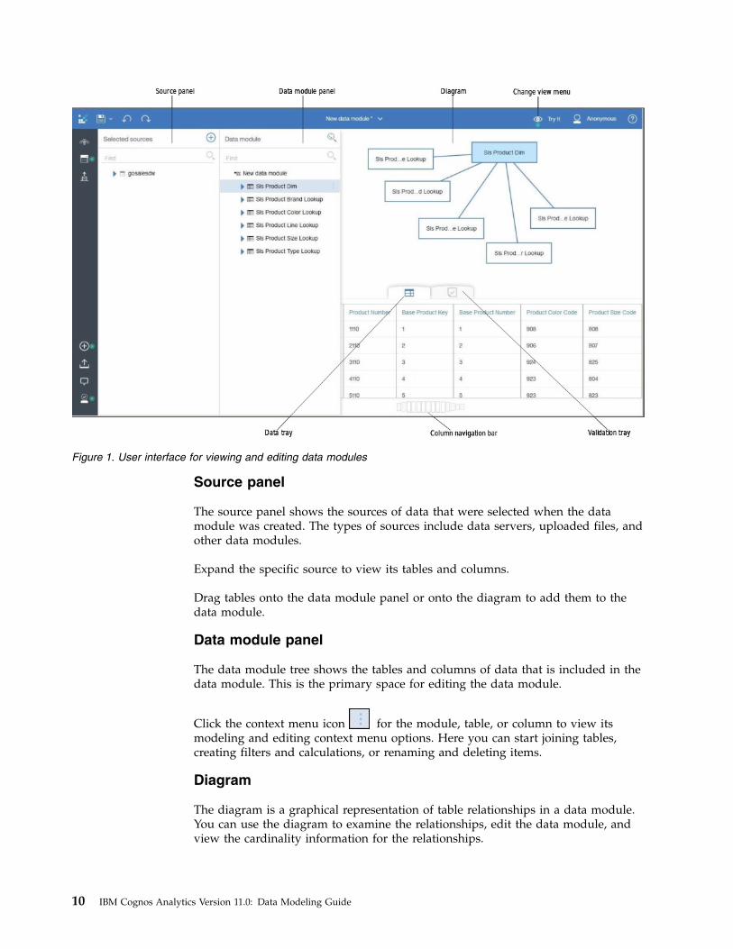
Source panel

The source panel shows the sources of data that were selected when the datamodule was created. The types of sources include data servers, uploaded files, andother data modules.

Expand the specific source to view its tables and columns.

Drag tables onto the data module panel or onto the diagram to add them to thedata module.

Data module panel

The data module tree shows the tables and columns of data that is included in thedata module. This is the primary space for editing the data module.

Click the context menu icon

for the module, table, or column to view itsmodeling and editing context menu options. Here you can start joining tables,creating filters and calculations, or renaming and deleting items.

Diagram

The diagram is a graphical representation of table relationships in a data module.You can use the diagram to examine the relationships, edit the data module, andview the cardinality information for the relationships.

Figure 1. User interface for viewing and editing data modules


Right-click a table in the diagram to view the table context menu that can be yourstarting point for creating joins or filters, renaming the table, viewing the tableproperties, or removing it from the module.

Click any table join to see the join summary information that includes thematching keys. When you right-click the join line, the context menu appears withoptions for editing or deleting the join.

Click the change view icon

in the application toolbar. In the box thatappears, select the Cardinality check box. The diagram now shows the cardinalityof relationships between different tables in your data module. Move the Degreesof separation slider. Depending on the slider position, the diagram shows differentdistances of relationships between tables.

Data tray

You can use the data tray to view the actual data in table columns and rows.

Select a table in the data module tree or in the diagram, and click the data tray

icon

to open the data tray.

To navigate between rows of data, drag the data tray icon up and down. Tonavigate between the columns of data, use the column navigation bar at thebottom of the data tray. To close the data tray, click its icon again.

Validation tray

You can use the validation tray to view errors that are identified by the validationprocess.

The messages are displayed after you start the Validate operation anywhere in the

modeling user interface, and the failed validation

icon is displayed for tables,columns, expressions, or joins where errors are discovered.

To open or close the validation tray, click its icon . To expand the message

viewing area, drag the tray icon

up.

RelationshipsA relationship joins logically related objects that the users want to combine in asingle query. Relationships exist between two tables.

You can modify or delete relationships, or create new ones so that the data moduleproperly represents the logical structure of your business. Verify that therelationships that you require exist in the data module, the cardinality is setcorrectly, and referential integrity is enforced.

The diagram provides a graphical view of table relationships in a data module.You can use the diagram to examine the relationships, create and edit the joins, orview the join cardinality.

Chapter 4. Refining a data module 11

Creating a relationship from scratchYou need to create relationships whenever the required relationships are notdetected by the IBM Cognos software.

About this task

Relationships can be created between tables from the same source and fromdifferent sources.

The diagram is the most convenient place to view all data module relationships,and quickly discover the disconnected tables.

Tip: The list of possible keys in the relationship editor excludes measures. Thismeans that if a row in a column was misidentified as a measure, but you want touse it as an identifier, you will not see the row in the key drop-down list. You needto examine the data module to confirm that the usage property is correct on eachcolumn in the table.

Procedure1. In the data module tree or in the diagram, click the table for which you want to

create a relationship, and from the context menu, click Join.

Tip: You can also start creating a relationship using the following methods:v In the data module tree or in the diagram, control-click the two tables that

you want to join in a relationship, and click Join.v On the Relationships tab in the table properties, click Create new.If the data module does not include the table that you need, you can drag thistable from Selected sources directly onto the diagram.

2. In the relationship editor, specify the second table to include in the relationship,and then select the matching columns in both tables.Depending on the method that you used to start the relationship, the secondtable might already be added, and you only need to match the columns. Youcan include more than one set of matching rows in both tables.

3. Specify the Join type for the relationship by selecting one of the availableoptions.

4. Specify the Cardinality of the relationship by selecting one of the availableoptions.

5. Specify the Filter join. If you apply this filter, the performance of a join can beimproved by filtering one side of the join with the values that are retrieved bythe other side.

6. Click OK.

Results

The new relationship appears on the Relationships tab in the properties page ofthe tables that you joined, and in the diagram view.

To view or edit all relationships defined for a table, go to the Relationships tab inthe table properties. To edit a relationship, click its expression, and make themodifications. To view a relationship from the diagram, click the join line to open asmall graphical view of the relationship. To edit a relationship from the diagram,right-click the join line, and click Edit.


To delete a relationship for a table, go to the Relationships tab in the table

properties, and click Edit. Then, click the remove icon

for the requiredrelationship, and click Done. To delete the relationship from the diagram,right-click the line joining the two tables, and click Remove.

CalculationsCalculations allow you to answer questions that cannot be answered by the sourcecolumns.

The following product functionality that you can use to refine your data modulesis based on underlying calculations:v Basic arithmetic calculations and field concatenations.v Custom groups.v Cleaning text data.v Custom calculations.

Creating basic calculationsYou can create basic arithmetic calculations for columns with numeric data types,and concatenate text values for columns with the text data type.

About this task

The expression for these calculations is predefined and you only need to select it.For example, you can create a column Revenue by multiplying values for Quantityand Unit price. You can create a column Name by combining two columns: Firstname and Last name.

Procedure1. To create a simple arithmetic calculation for columns with numeric data types,

use the following steps:a. In the data module tree, right-click the column for which you want to create

a calculation. For calculations that are based on two columns, usecontrol-click to select the columns.

b. In the Create a calculation box, type a name for the calculation.c. If the calculation is based on one column, type the number to use in the

calculation.d. Click Create.

2. To create a calculation that concatenates values for columns with the text datatype, use the following steps:a. In the data module tree, control-click the two columns that you want to

combine into a single column. Depending on which column you select first,its value appears at the beginning of the combined string.

b. Click Create a calculation, and select the suggested option.c. Type a name for the calculation.d. Click Create.

Results

In the table that you added the calculation to, you can now see a new column withthe new calculation at the end of the list of columns. An expression for the


calculation is automatically created in the expression editor. To view theexpression, go to the column properties page and click on the expression that isshown for the Expression property.

Grouping dataYou can organize the column data into custom groups so that the data is easier toread and analyze.

About this task

You can create two types of custom groups depending on the data type of thecolumn: one group type for columns with numeric data and the second group typefor columns with text data. For example, in the Employee code column you cangroup employees into ranges, such as 0-100, 101-200, 200+. In the Manager column,you can group managers according to their rank, such as First line manager,Senior manager, and so on.

Procedure1. In the data module tree, right-click the column that you want to group on, and

click Custom groups.2. If you selected a numeric column, specify the grouping in the following way:

a. Specify how many groups you want to create.b. Specify the distribution of the values to be either Equal distribution or

Custom.c. If you chose Equal distribution, specify the values to be contained in each

group by typing the numbers or clicking the scroll bars.d. If you chose Custom, you can enter your own range values for the group.e. Optional: Change the group name.f. Click Create.

3. If you selected a text column, specify the grouping in the following way:a. Control-select the values to include in the first group.b. In the Groups column, click the plus sign.c. Specify the name for the group, and click OK. The values are added in the

Group members column, and the name of the group appears in the Groupscolumn. You can add additional values to a group after it is created, andyou can remove values from a group. You can also remove a group.

d. Optional: To add another group, repeat the steps for the first group.e. Optional: To create a group that contains all of the values that aren't already

included in a group, select the Group remaining and future values incheck box, and specify a name for the group.

f. Click Create.

Results

The custom group column that is based on your selections appears at the end ofthe list of columns in the table. A group expression is automatically created in theexpression editor. To view the expression, go to the column properties page andclick on the expression that is shown for the Expression property.

Tip: To complete the action of creating the custom group, you can click Replaceinstead of Create. This option will replace the column name in the table with thegroup name.


Cleaning dataData is often messy and inconsistent. You might want to impose some formattingorder on your data so that it's clearer and easier to read.

About this task

The Clean options that are available for a column depend on the column datatype. Some options can be specified for multiple columns with the same data type,and some for singular columns only.

The following options are available to clean your data:

WhitespaceTrim leading and trailing whitespace

Select this check box to remove leading and trailing whitespace fromstrings.

Convert case toUPPERCASE, lowercase, Do not change

Use this option to change the case of all characters in the string to eitheruppercase or lowercase, or to ensure that the case of each individualcharacter is unchanged.

Return a substring of charactersReturn a string that includes only part of the original string in each value.For example, an employee code can be stored as CA096670, but you needonly the number 096670 so you use this option to remove the CA part. Youcan specify this option for singular columns only.

For the Start value, type a number that represents the position of acharacter in the string that will start the substring. Number 1 representsthe first character in the string. For the Length value, specify the numberof characters that will be included in the substring.

NULL values

Specify NULL-handling options for columns with text, numeric, date, andtime data types that allow NULL values. When Cognos Analytics detectsthat a column does not allow NULL values, these options are not availablefor that column.The default value for each option depends on the column data type. Fortext data, the default is an empty string. For numbers, the default is 0. Fordates, the default is 2000-01-01. For time, the default is 12:00:00. For dateand time (timestamp), the default is 2000-01-01T12:00:00.The entry field for each option also depends on the column data type. Fortext, the entry field accepts alphanumeric characters, for numbers, theentry field accepts only numeric input. For dates, a date picker is providedto select the date, and for time, a time picker is provided to select the time.The following NULL-handling options are available:

Replace this value with NULLReplaces the text, numbers, date, and time values, as you specify in theentry field, with NULL.For example, if you want to use an empty string instead of NULL in agiven column, but your uploaded file sometimes uses the string n/a toindicate that the value is unknown, you can replace n/a with NULL, andthen choose to replace NULL with the empty string.


Replace NULL values withReplaces NULL values with text, numbers, date, and time values, as youspecify in the entry field.For example, for the Middle Name column, you can specify the followingvalues to be used for cells where middle name does not exist: n/a, none, orthe default empty string. For the Discount Amount column, you canspecify 0.00 for cells where the amount is unknown.

Procedure

1. In the data module tree, click the context menu icon

for a column, andclick Clean.

Tip: To clean data in multiple columns at once, control-select the columns thatyou want to clean. The Clean option is available only if the data type of eachselected column is the same.

2. Specify the options that are applicable for the selected column or columns.3. Click Clean.

Results

After you complete the Clean operation, the expression editor automatically createsan expression for the modified column or columns. To view the expression, openthe column properties panel, and click the expression that is shown for theExpression property.

Creating custom calculationsTo create a custom calculation, you must define your own expression using theexpression editor.

About this task

Custom calculations can be created at the data module level or at the table level.The module-level calculations can reference columns from multiple tables.

For information about the functions that you can use to define your expressions,see Appendix A, “Using the expression editor,” on page 23.

Procedure1. In the data module tree, right-click the data module name or a specific table

name, and click Create custom calculation.2. In the Expression editor panel, define the expression for your calculation, and

specify a name for it.v To enter a function for your expression, type the first character of the

function name, and select the function from the drop-down list of suggestedfunctions.

v To add table columns to your expression, drag-and-drop one or morecolumns from the data module tree to the expression editor panel. Thecolumn name is added where you place the cursor in the expression editor.

Tip: You can also double-click the column in the data module tree, and thecolumn name appears in the expression editor.

3. Click Validate to check if the expression is valid.


4. After successful validation, click OK.

Results

If you created your calculation at the data module level, the calculation is addedafter the last table in the data module tree. If you created your calculation at thetable level, the calculation is added at the end of the list of columns in the table. Toview the expression for the calculation, open the calculation properties panel, andclick on the expression that is shown for the Expression property.

Creating navigation groups

A navigation group is a collection of non-measure columns that business usersmight associate for data exploration.

When a data module contains navigation groups, the dashboard users can drilldown and back to change the focus of their analysis by moving between levels ofinformation. The users can drill down from column to column in the navigationgroup by either following the order of columns in the navigation group, or bychoosing the column to which they want to proceed.

About this task

You can create a navigation group with columns that are logically related, such asyear, month, quarter, week. You can also create a navigation group with columnsthat are not logically related, such as product, customer, state, city.

Columns from different tables can be added to a navigation group. The samecolumn can be added to multiple navigation groups.

Procedure1. In the data module panel, start creating a navigation group by using one of the

following methods:

v From the data module context menu , click Properties, and then click theNavigation groups tab. Click Add a navigation group, and drag columnsfrom the data module panel to the Create navigation group panel.

v In the data module tree, select one or more columns, and from the context

menu

of any of the selected columns, click Create navigation group.

The selected columns are listed in the Create navigation group panel. If thereare multiple columns, the name of the navigation group includes names of thefirst and last column in the group.

2. If needed, modify the navigation group in the following way:v To add different columns, drag the columns from the data module panel to

the navigation group panel. You can multi-select columns and drag them allat once.

v To remove columns, click the remove

icon for the column.v To change the order of columns, drag them up or down.v To change the navigation group name, overwrite the default name.


The default name reacts to the changed order of columns. If you override thedefault name, it does no longer change when you modify the groupdefinition. The name cannot be blank.

3. Click Apply, and save the data module.

If you select the option Identify navigation group members in the datamodule toolbar, the columns that are members of navigation groups areunderlined.

Results

The navigation group is added to the data module and will be available to users indashboards and stories.

What to do next

The modeler can modify navigation groups at any time, and re-save the datamodule.

To view the navigation group or groups that a column belongs to, from the column

context menu , click Properties > Navigation groups. Click the navigationgroup name to view or modify its definition.

To view all navigation groups in a data module, from the data module context

menu , click Properties > Navigation groups. Click the navigation groupnames to view or modify their definitions. To delete a navigation group, click

Remove, click the remove

icon for the group, and click Done.

Filtering dataA filter specifies the conditions that rows must meet to be retrieved from a table.

About this task

The filter is based on a specific column in a table, but it affects the whole table.Also, only rows that meet the filter criteria are retrieved from other tables.

You can create filters at the table level, which allows you to add multiple filters atonce, or at the column level.

Procedure1. In the data module tree or in the diagram, locate the table for which you want

to create filters.

v To create a filter at the table level, click the table context menu icon , andthen click Filter.

Tip: You can also right-click the table in the diagram, and click Filter fromthere.On the Filters tab in the table properties pane, click Add a filter, select acolumn, and click Enter a value.

v To create a filter at the column level, expand the table in the data module

panel, and from the column context menu , click Filter.


2. Select the filter values in the following way:a. If the column data type is integer, you have two options to specify the

values: Range and Individual values. When you choose Range, use theslider to specify the value ranges. When you choose Individual values,select the check boxes associated with the values.

b. For columns with numeric data types other than integer, use the slider tospecify the range values.

c. For columns with date and time (timestamp) data types, specify a range ofvalues before, after, or between the selected date and time, or selectindividual values.

d. For columns with text data types, select the check boxes associated with thevalues.

3. Optional: To select values that are outside the range that you specified, clickInvert.

4. Specify a meaningful label for the filter.5. Click Apply.

Results

After you create a filter, the filter icon

is added for the table and column in thedata module panel and in the diagram.

What to do next

To view, edit, or remove the filters defined for a table, go to the Filters tab in thetable properties. To edit the filter, click its expression, make the modifications, andclick Done.

Tip: To edit a filter on a single column, from the column context menu

in thedata module panel, click Filter to open the filter definition.

To remove any filter from a table, go to the Filters tab in the table properties, and

click Edit. Then, click the remove icon

that appears before the filter name, andclick Done.

Hiding tables and columns

You can hide a table or column in a data module. The hidden tables or columnsremain visible in the modeling interface, but they are not visible in the reportingand dashboarding interfaces. The hidden items are fully functional in the product.

About this task

Use this feature to provide an uncluttered view of metadata for the report anddashboard users. For example, when you hide columns that are referenced in acalculation, the metadata tree in the reporting and dashboarding interfaces showsonly the calculation column, but not the referenced columns. When you hide theidentifier columns used as keys for joins, the keys are not exposed in thedashboarding and reporting interfaces, but the joins are functional in all interfaces.


Procedure

1. In the data module tree, click the context menu icon

for a table or column,and click Hide.You can also select multiple tables or columns to hide them at once.

Tip: To un-hide the items, click the context menu icon for the hidden table orcolumn, and click Show.

2. Save the data module.

Results

The labels on the hidden tables and columns are grayed out in the data moduletree and in the diagram. Also, on the General tab of the table or columnproperties, the check box This item is hidden from users is selected.

The hidden tables and columns are not visible in the reporting and dashboardinginterfaces.

Validating data modules

Use the validation feature to check for invalid object references within a datamodule.

About this task

Validation identifies the following errors:v A table or column that a data module is based on no longer exists in the source.v A calculation expression is invalid.v A filter references a column that no longer exists in the data module.v A table or column that is referenced in a join no longer exists in the data

module.

Errors in the data module are identified by the failed validation icon . The

descriptions of errors are shown in the validation tray when it is open .

Procedure

1. In the data module tree, click the data module context menu icon , andclick Validate

If errors are identified, the failed validation icon

is displayed in the datamodule tree, in the diagram, and in the properties panel, next to the column orexpression where the error exists. The descriptions of errors are displayed inthe validation tray.

Tip: To open or close the validation tray, click its icon .


2. Click the failed validation

icon for a module, column, expression, or join toview a pop-up box that informs you of the number of errors for the selected

item. Double-click the failed validation icon in the pop-up box to view theerror details.

Results

Using the validation messages, try to resolve the errors. You can save a datamodule with validation errors in it.


Appendix A. Using the expression editor

An expression is any combination of operators, constants, functions, and othercomponents that evaluates to a single value. You build expressions to createcalculation and filter definitions. A calculation is an expression that you use tocreate a new value from existing values that are contained within a data item. Afilter is an expression that you use to retrieve a specific subset of records.

OperatorsOperators specify what happens to the values on either side of the operator.Operators are similar to functions, in that they manipulate data items and return aresult.

(Identifies the beginning of an expression.

Syntax( expression )

)Identifies the end of an expression.

Syntax( expression )

*Multiplies two numeric values.

Syntaxvalue1 * value2

/Divides two numeric values.

Syntaxvalue1 / value2

||Concatenates, or joins, strings.

Syntaxstring1 || string2

+Adds two numeric values.

Syntaxvalue1 + value2


-Subtracts two numeric values or negates a numeric value.

Syntaxvalue1 - value2or- value

<Compares the values that are represented by "value1" against "value2" andretrieves the values that are less than "value2".

Syntaxvalue1 < value2

<=Compares the values that are represented by "value1" against "value2" andretrieves the values that are less than or equal to "value2".

Syntaxvalue1 <= value2

<>Compares the values that are represented by "value1" against "value2" andretrieves the values that are not equal to "value2".

Syntaxvalue1 <> value2

=Compares the values that are represented by "value1" against "value2" andretrieves the values that are equal to "value2".

Syntaxvalue1 = value2

>Compares the values that are represented by "value1" against "value2" andretrieves the values that are greater than "value2".

Syntaxvalue1 > value2

>=Compares the values that are represented by "value1" against "value2" andretrieves the values that are greater than or equal to "value2".

Syntaxvalue1 >= value2


andReturns "true" if the conditions on both sides of the expression are true.

Syntaxargument1 and argument2

betweenDetermines if a value falls in a given range.

Syntaxexpression between value1 and value2

Example[Revenue] between 200 and 300

Result

Returns the number of results with revenues between 200 and 300.

Result data

Revenue Between$332.06 false$230.55 true$107.94 false

caseWorks with when, then, else, and end. Case identifies the beginning of a specificsituation, in which when, then, and else actions are defined.

Syntaxcase expression { when expression then expression } [ elseexpression ] end

containsDetermines if "string1" contains "string2".

Syntaxstring1 contains string2

distinctA keyword used in an aggregate expression to include only distinct occurrences ofvalues. See also the function unique.

Syntaxdistinct dataItem

Examplecount ( distinct [OrderDetailQuantity] )

Result

Appendix A. Using the expression editor 25

1704

elseWorks with the if or case constructs. If the if condition or the case expression arenot true, then the else expression is used.

Syntaxif ( condition ) then .... else ( expression ) , or case .... else (expression ) end

endIndicates the end of a case or when construct.

Syntaxcase .... end

ends withDetermines if "string1" ends with "string2".

Syntaxstring1 ends with string2

ifWorks with the then and else constructs. If defines a condition; when the ifcondition is true, the then expression is used. When the if condition is not true, theelse expression is used.

Syntaxif ( condition ) then ( expression ) else ( expression )

inDetermines if "expression1" exists in a given list of expressions.

Syntaxexpression1 in ( expression_list )

is missingDetermines if "value" is undefined in the data.

Syntaxvalue is missing

likeDetermines if "string1" matches the pattern of "string2", with the character "char"optionally used to escape characters in the pattern string.

Syntaxstring1 LIKE string2 [ ESCAPE char ]


Example 1[PRODUCT_LINE] like ’G%’

Result

All product lines that start with 'G'.

Example 2[PRODUCT_LINE] like ’%Ga%’ escape ’a’

Result

All the product lines that end with 'G%'.

lookupFinds and replaces data with a value you specify. It is preferable to use the caseconstruct.

Syntaxlookup ( name ) in ( value1 --> value2 ) default ( expression )

Examplelookup ( [Country]) in ( ’Canada’--> ( [List Price] * 0.60),’Australia’--> ( [List Price] * 0.80 ) ) default ( [List Price] )

notReturns TRUE if "argument" is false or returns FALSE if "argument" is true.

SyntaxNOT argument

orReturns TRUE if either of "argument1" or "argument2" are true.

Syntaxargument1 or argument2

starts withDetermines if "string1" starts with "string2".

Syntaxstring1 starts with string2

thenWorks with the if or case constructs. When the if condition or the when expressionare true, the then expression is used.

Syntaxif ( condition ) then ..., or case expression when expressionthen .... end


whenWorks with the case construct. You can define conditions to occur when theWHEN expression is true.

Syntaxcase [expression] when ... end

SummariesThis list contains predefined functions that return either a single summary valuefor a group of related values or a different summary value for each instance of agroup of related values.

Statistical functionsThis list contains predefined summary functions of statistical nature.

standard-deviationReturns the standard deviation of selected data items.

Syntaxstandard-deviation ( expression [ auto ] )standard-deviation ( expression for [ all|any ] expression { ,expression } )standard-deviation ( expression for report )

Examplestandard-deviation ( ProductCost )

Result

Returns a value indicating the deviation between product costs and the averageproduct cost.

varianceReturns the variance of selected data items.

Syntaxvariance ( expression [ auto ] )variance ( expression for [ all|any ] expression { , expression } )variance ( expression for report )

Examplevariance ( Product Cost )

Result

Returns a value indicating how widely product costs vary from the averageproduct cost.

averageReturns the average value of selected data items. Distinct is an alternativeexpression that is compatible with earlier versions of the product.


Syntaxaverage ( [ distinct ] expression [ auto ] )average ( [ distinct ] expression for [ all|any ] expression { ,expression } )average ( [ distinct ] expression for report )

Exampleaverage ( Sales )

Result

Returns the average of all Sales values.

countReturns the number of selected data items excluding null values. Distinct is analternative expression that is compatible with earlier versions of the product. All issupported in DQM mode only and it avoids the presumption of double counting adata item of a dimension table.

Syntaxcount ( [ all | distinct ] expression [ auto ] )count ( [ all | distinct ] expression for [ all|any ] expression { ,expression } )count ( [ all | distinct ] expression for report )

Examplecount ( Sales )

Result

Returns the total number of entries under Sales.

maximumReturns the maximum value of selected data items. Distinct is an alternativeexpression that is compatible with earlier versions of the product.

Syntaxmaximum ( [ distinct ] expression [ auto ] )maximum ( [ distinct ] expression for [ all|any ] expression { ,expression } )maximum ( [ distinct ] expression for report )

Examplemaximum ( Sales )

Result

Returns the maximum value out of all Sales values.

medianReturns the median value of selected data items.


Syntaxmedian ( expression [ auto ] )median ( expression for [ all|any ] expression { , expression } )median ( expression for report )

minimumReturns the minimum value of selected data items. Distinct is an alternativeexpression that is compatible with earlier versions of the product.

Syntaxminimum ( [ distinct ] expression [ auto ] )minimum ( [ distinct ] expression for [ all|any ] expression { ,expression } )minimum ( [ distinct ] expression for report )

Exampleminimum ( Sales )

Result

Returns the minimum value out of all Sales values.

percentageReturns the percent of the total value for selected data items. The "<for-option>"defines the scope of the function. The "at" option defines the level of aggregationand can be used only in the context of relational datasources.

Syntaxpercentage ( numeric_expression [ at expression { , expression } ][ <for-option> ] [ prefilter ] )percentage ( numeric_expression [ <for-option> ] [ prefilter ] )<for-option> ::= for expression { , expression }|for report|auto

Examplepercentage ( Sales 98 )

Result

Returns the percentage of the total sales for 1998 that is attributed to each salesrepresentative.

Result data

Employee Sales 98 PercentageGibbons 60646 7.11%Flertjan 62523 7.35%Cornel 22396 2.63%

percentileReturns a value, on a scale of one hundred, that indicates the percent of adistribution that is equal to or below the selected data items. The "<for-option>"defines the scope of the function. The "at" option defines the level of aggregationand can be used only in the context of relational datasources.


Syntaxpercentile ( numeric_expression [ at expression { , expression } ][ <for-option> ] [ prefilter ] )percentile ( numeric_expression [ <for-option> ] [ prefilter ] )<for-option> ::= for expression { , expression }|for report|auto

Examplepercentile ( Sales 98 )

Result

For each row, returns the percentage of rows that are equal to or less than thequantity value of that row.

Result data

Qty Percentile (Qty)800 1700 0.875600 0.75500 0.625400 0.5400 0.5200 0.25200 0.25

quantileReturns the rank of a value within a range that you specify. It returns integers torepresent any range of ranks, such as 1 (highest) to 100 (lowest). The"<for-option>" defines the scope of the function. The "at" option defines the level ofaggregation and can be used only in the context of relational datasources.

Syntaxquantile ( numeric_expression , numeric_expression [ at expression { ,expression } ] [ <for-option> ] [ prefilter ] )quantile ( numeric_expression , numeric_expression [ <for-option> ][ prefilter ] )<for-option> ::= for expression { , expression }|for report|auto

Examplequantile ( Qty , 4 )

Result

Returns the quantity, the rank of the quantity value, and the quantity valuesbroken down into 4 quantile groups (quartiles).

Result data

Qty Rank Quantile (Qty, 4)800 1 1700 2 1600 3 2500 4 2400 5 3


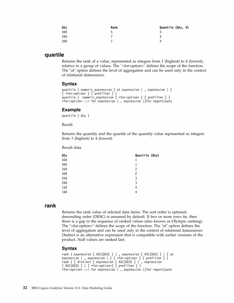
Qty Rank Quantile (Qty, 4)400 5 3200 7 4200 7 4

quartileReturns the rank of a value, represented as integers from 1 (highest) to 4 (lowest),relative to a group of values. The "<for-option>" defines the scope of the function.The "at" option defines the level of aggregation and can be used only in the contextof relational datasources.

Syntaxquartile ( numeric_expression [ at expression { , expression } ][ <for-option> ] [ prefilter ] )quartile ( numeric_expression [ <for-option> ] [ prefilter ] )<for-option> ::= for expression { , expression }|for report|auto

Examplequartile ( Qty )

Result

Returns the quantity and the quartile of the quantity value represented as integersfrom 1 (highest) to 4 (lowest).

Result data

Qty Quartile (Qty)450 1400 1350 2300 2250 3200 3150 4100 4

rankReturns the rank value of selected data items. The sort order is optional;descending order (DESC) is assumed by default. If two or more rows tie, thenthere is a gap in the sequence of ranked values (also known as Olympic ranking).The "<for-option>" defines the scope of the function. The "at" option defines thelevel of aggregation and can be used only in the context of relational datasources.Distinct is an alternative expression that is compatible with earlier versions of theproduct. Null values are ranked last.

Syntaxrank ( expression [ ASC|DESC ] { , expression [ ASC|DESC ] } [ atexpression { , expression } ] [ <for-option> ] [ prefilter ] )rank ( [ distinct ] expression [ ASC|DESC ] { , expression[ ASC|DESC ] } [ <for-option>] [ prefilter ] )<for-option> ::= for expression { , expression }|for report|auto


Examplerank ( Sales 98 )

Result

For each row, returns the rank value of sales for 1998 that is attributed to eachsales representative. Some numbers are skipped when a tie between rows occurs.

Result data

Employee Sales 98 RankGibbons 60000 1Flertjan 50000 2Cornel 50000 2Smith 48000 4

tertileReturns the rank of a value as High, Middle, or Low relative to a group of values.

Syntaxtertile ( expression [ auto ] )tertile ( expression for [ all|any ] expression { , expression } )tertile ( expression for report )

Exampletertile ( Qty )

Result

Returns the quantity, the quantile rank value of the quantity as broken down intotertiles, and the quantile rank label as broken down into tertiles.

Result data

Qty Quantile (Qty, 3) Tertile (Qty)800 1 H700 1 H500 2 M400 2 M200 3 L200 3 L

totalReturns the total value of selected data items. Distinct is an alternative expressionthat is compatible with earlier versions of the product.

Syntaxtotal ( [ distinct ] expression [ auto ] )total ( [ distinct ] expression for [ all|any ] expression { ,expression } )total ( [ distinct ] expression for report )


Exampletotal ( Sales )

Result

Returns the total value of all Sales values.

Business Date/Time FunctionsThis list contains business functions for performing date and time calculations.

_add_secondsReturns the time or datetime, depending on the format of "time_expression", thatresults from adding "integer_expression" seconds to "time_expression".

Syntax_add_seconds ( time_expression, integer_expression )

Example 1_add_seconds ( 13:04:59 , 1 )

Result

13:05:00

Example 2_add_seconds ( 2002-04-30 12:10:10.000, 1 )

Result

2002-04-30 12:10:11.000

Example 3_add_seconds ( 2002-04-30 00:00:00.000, 1/100 )Note that the secondargument is not a whole number. This is supported by some databasetechnologies and increments the time portion.

Result

2002-04-30 00:00:00.010

_add_minutesReturns the time or datetime, depending on the format of "time_expression", thatresults from adding "integer_expression" minutes to "time_expression".

Syntax_add_minutes ( time_expression, integer_expression )

Example 1_add_minutes ( 13:59:00 , 1 )

Result


14:00:00

Example 2_add_minutes ( 2002-04-30 12:59:10.000, 1 )

Result

2002-04-30 13:00:10.000

Example 3_add_minutes ( 2002-04-30 00:00:00.000, 1/60 )Note that the secondargument is not a whole number. This is supported by some databasetechnologies and increments the time portion.

Result

2002-04-30 00:00:01.000

_add_hoursReturns the time or datetime, depending on the format of "time_expression", thatresults from adding "integer_expression" hours to "time_expression".

Syntax_add_hours ( time_expression, integer_expression )

Example 1_add_hours ( 13:59:00 , 1 )

Result

14:59:00

Example 2_add_hours ( 2002-04-30 12:10:10.000, 1 )

Result

2002-04-30 13:10:10.000,

Example 3_add_hours ( 2002-04-30 00:00:00.000, 1/60 )Note that the secondargument is not a whole number. This is supported by some databasetechnologies and increments the time portion.

Result

2002-04-30 00:01:00.000

_add_daysReturns the date or datetime, depending on the format of "date_expression", thatresults from adding "integer_expression" days to "date_expression".


Syntax_add_days ( date_expression, integer_expression )

Example 1_add_days ( 2002-04-30 , 1 )

Result

2002-05-01

Example 2_add_days ( 2002-04-30 12:10:10.000, 1 )

Result

2002-05-01 12:10:10.000

Example 3_add_days ( 2002-04-30 00:00:00.000, 1/24 )Note that the secondargument is not a whole number. This is supported by some databasetechnologies and increments the time portion.

Result

2002-04-30 01:00:00.000

_add_monthsAdds "integer_expression" months to "date_expression". If the resulting month hasfewer days than the day of month component, then the last day of the resultingmonth is returned. In all other cases the returned value has the same day of monthcomponent as "date_expression".

Syntax_add_months ( date_expression, integer_expression )

Example 1_add_months ( 2012-04-15 , 3 )

Result

2012-07-15


Result

2012-03-29

Example 3_last_of_month ( _add_months ( 2012-02-29 , 1 ) )

Result


2012-03-31


Result

2012-02-29

Example 5_add_months ( 2002-04-30 12:10:10.000 , 1 )

Result

2002-05-30 12:10:10.000

_add_yearsAdds "integer_expression" years to "date_expression". If the "date_expression" isFebruary 29 and resulting year is non leap year, then the resulting day is set toFebruary 28. In all other cases the returned value has the same day and month as"date_expression".

Syntax_add_years ( date_expression, integer_expression )

Example 1_add_years ( 2012-04-15 , 1 )

Result

2013-04-15

Example 2_add_years ( 2012-02-29 , 1 )

Result

2013-02-28

Example 3_add_years ( 2002-04-30 12:10:10.000 , 1 )

Result

2003-04-30 12:10:10.000

_ageReturns a number that is obtained from subtracting "date_expression" from today'sdate. The returned value has the form YYYYMMDD, where YYYY represents thenumber of years, MM represents the number of months, and DD represents thenumber of days.

Syntax_age ( date_expression )


Example_age ( 1990-04-30 ) (if today’s date is 2003-02-05)

Result

120906, meaning 12 years, 9 months, and 6 days.

current_dateReturns a date value representing the current date of the computer that thedatabase software runs on.

Syntaxcurrent_date

Examplecurrent_date

Result

2003-03-04

current_timeReturns a time with time zone value, representing the current time of the computerthat runs the database software if the database supports this function. Otherwise, itrepresents the current time of the IBM Cognos Analytics server.

Syntaxcurrent_time

Examplecurrent_time

Result

16:33:11.354+05:00

current_timestampReturns a datetime with time zone value, representing the current time of thecomputer that runs the database software if the database supports this function.Otherwise, it represents the current time of the server.

Syntaxcurrent_timestamp

Examplecurrent_timestamp

Result

2003-03-03 16:40:15.535+05:00


_day_of_weekReturns the day of week (1 to 7), where 1 is the first day of the week as indicatedby the second parameter (1 to 7, 1 being Monday and 7 being Sunday). Note thatin ISO 8601 standard, a week begins with Monday being day 1.

Syntax_day_of_week ( date_expression, integer )

Example_day_of_week ( 2003-01-01 , 1 )

Result

3

_day_of_yearReturns the day of year (1 to 366) in "date_ expression". Also known as Julian day.

Syntax_day_of_year ( date_expression )

Example_day_of_year ( 2003-03-01 )

Result

61

_days_betweenReturns a positive or negative number representing the number of days between"date_expression1" and "date_expression2". If "date_expression1" <"date_expression2", then the result will be a negative number.

Syntax_days_between ( date_expression1 , date_expression2 )

Example_days_between ( 2002-04-30 , 2002-06-21 )

Result

-52

_days_to_end_of_monthReturns a number representing the number of days remaining in the monthrepresented by "date_expression".

Syntax_days_to_end_of_month ( date_expression )


Example_days_to_end_of_month ( 2002-04-20 14:30:22.123 )

Result

10

_end_of_dayReturns the end of today as a timestamp.

Syntax_end_of_day

Example_end_of_day

Result2014-11-23 23:59:59

_first_of_monthReturns a date or datetime, depending on the argument, by converting"date_expression" to a date with the same year and month but with the day set to1.

Syntax_first_of_month ( date_expression )

Example 1_first_of_month ( 2002-04-20 )

Result

2002-04-01

Example 2_first_of_month ( 2002-04-20 12:10:10.000 )

Result

2002-04-01 12:10:10.000

_from_unixtimeReturns the unix time specified by an integer expression as a timestamp with timezone.

Syntax_from_unixtime ( integer_expression )

Example_from_unixtime ( 1417807335 )

Result2014-12-05 19:22:15+00:00


_hourReturns the value of the hour field in a date expression.

Syntax_hour( date_expression )

Example_hour ( 2002-01-31 12:10:10.254 )

Result12

_last_of_monthReturns a date or datetime, depending on the argument, that is the last day of themonth represented by "date_expression".

Syntax_last_of_month ( date_expression )

Example 1_last_of_month ( 2002-01-14 )

Result

2002-01-31

Example 2_last_of_month ( 2002-01-14 12:10:10.000 )

Result

2002-01-31 12:10:10.000

_make_timestampReturns a timestamp constructed from "integer_expression1" (the year),"integer_expression2" (the month), and "integer_expression3" (the day). The timeportion defaults to 00:00:00.000 .

Syntax_make_timestamp ( integer_expression1, integer_expression2,integer_expression3 )

Example_make_timestamp ( 2002 , 01 , 14 )

Result

2002-01-14 00:00:00.000

_minuteReturns the value of the minute field in a date expression.


Syntax_minute( date_expression )

Example_minute ( 2002-01-31 12:10:10.254 )

Result10

_monthReturns the value of the month field in a date expression.

Syntax_month( date_expression )

Example_month ( 2003-03-01 )

Result3

_months_betweenReturns a positive or negative integer number representing the number of monthsbetween "date_expression1" and "date_expression2". If "date_expression1" is earlierthan "date_expression2", then a negative number is returned.

Syntax_months_between ( date_expression1, date_expression2 )

Example_months_between ( 2002-04-03 , 2002-01-30 )

Result

2

_secondReturns the value of the second field in a date expression.

Syntax_second( date_expression )

Example_second ( 2002-01-31 12:10:10.254 )

Result10.254

_shift_timezoneShifts a timestamp value from one time zone to another time zone. This functionhonors the Daylight Savings Time when applicable. If the first argument is of type"timestamp", then the second and third arguments represent the "from" and


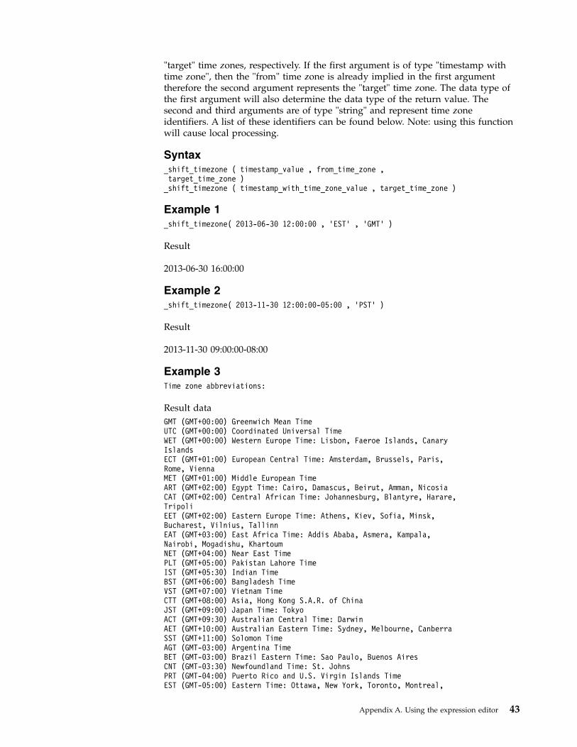
"target" time zones, respectively. If the first argument is of type "timestamp withtime zone", then the "from" time zone is already implied in the first argumenttherefore the second argument represents the "target" time zone. The data type ofthe first argument will also determine the data type of the return value. Thesecond and third arguments are of type "string" and represent time zoneidentifiers. A list of these identifiers can be found below. Note: using this functionwill cause local processing.

Syntax_shift_timezone ( timestamp_value , from_time_zone ,target_time_zone )_shift_timezone ( timestamp_with_time_zone_value , target_time_zone )

Example 1_shift_timezone( 2013-06-30 12:00:00 , ’EST’ , ’GMT’ )

Result

2013-06-30 16:00:00

Example 2_shift_timezone( 2013-11-30 12:00:00-05:00 , ’PST’ )

Result

2013-11-30 09:00:00-08:00

Example 3Time zone abbreviations:

Result dataGMT (GMT+00:00) Greenwich Mean TimeUTC (GMT+00:00) Coordinated Universal TimeWET (GMT+00:00) Western Europe Time: Lisbon, Faeroe Islands, CanaryIslandsECT (GMT+01:00) European Central Time: Amsterdam, Brussels, Paris,Rome, ViennaMET (GMT+01:00) Middle European TimeART (GMT+02:00) Egypt Time: Cairo, Damascus, Beirut, Amman, NicosiaCAT (GMT+02:00) Central African Time: Johannesburg, Blantyre, Harare,TripoliEET (GMT+02:00) Eastern Europe Time: Athens, Kiev, Sofia, Minsk,Bucharest, Vilnius, TallinnEAT (GMT+03:00) East Africa Time: Addis Ababa, Asmera, Kampala,Nairobi, Mogadishu, KhartoumNET (GMT+04:00) Near East TimePLT (GMT+05:00) Pakistan Lahore TimeIST (GMT+05:30) Indian TimeBST (GMT+06:00) Bangladesh TimeVST (GMT+07:00) Vietnam TimeCTT (GMT+08:00) Asia, Hong Kong S.A.R. of ChinaJST (GMT+09:00) Japan Time: TokyoACT (GMT+09:30) Australian Central Time: DarwinAET (GMT+10:00) Australian Eastern Time: Sydney, Melbourne, CanberraSST (GMT+11:00) Solomon TimeAGT (GMT-03:00) Argentina TimeBET (GMT-03:00) Brazil Eastern Time: Sao Paulo, Buenos AiresCNT (GMT-03:30) Newfoundland Time: St. JohnsPRT (GMT-04:00) Puerto Rico and U.S. Virgin Islands TimeEST (GMT-05:00) Eastern Time: Ottawa, New York, Toronto, Montreal,


Jamaica, Porto AcreCST (GMT-06:00) Central Time: Chicago, Cambridge Bay, Mexico CityMST (GMT-07:00) Mountain Time: Edmonton, Yellowknife, ChihuahuaPST (GMT-08:00) Pacific Time: Los Angeles, Tijuana, VancouverAST (GMT-09:00) Alaska Time: Anchorage, Juneau, Nome, YakutatHST (GMT-10:00) Hawaii Time: Honolulu, TahitiMIT (GMT-11:00) Midway Islands Time: Midway, Apia, Niue, Pago Pago

Example 4A customized time zone identifier may also be used, using the formatGMT(+|-)HH:MM. For example, GMT-06:30 or GMT+02:00.A more completelist of time zone idenfitiers (including longer form identifiers suchas "Europe/Amsterdam") may be found in the "i18n_res.xml" file fromthe product’s configuration folder.

_start_of_dayReturns the start of today as a timestamp.

Syntax_start_of_day

Example_start_of_day

Result

2014-11-23 00:00:00

_week_of_yearReturns the number of the week of the year of "date_expression" according to theISO 8601 standard. Week 1 of the year is the first week of the year to contain aThursday, which is equivalent to the first week containing January 4th. A weekstarts on Monday (day 1) and ends on Sunday (day 7).

Syntax_week_of_year ( date_expression )

Example_week_of_year ( 2003-01-01 )

Result

1

_timezone_hourReturns the value of the timezone hour field in a date expression.

Syntax_timezone_hour( date_expression )

Example_timezone_hour ( 2002-01-31 12:10:10.254-05:30 )

Result


5

_timezone_minuteReturns the value of the timezone minute field in a date expression.

Syntax_timezone_minute( date_expression )

Example_timezone_minute ( 2002-01-31 12:10:10.254-05:30 )

Result30

_unix_timestampReturns the unix time specified by an integer expression as a timestamp with timezone.

Syntax_unix_timestamp

Example_unix_timestamp

Result1416718800

_yearReturns the value of the year field in a date expression.

Syntax_year( date_expression )

Example_year ( 2003-03-01 )

Result2003

_years_betweenReturns a positive or negative integer number representing the number of yearsbetween "date_expression1" and "date_expression2". If "date_expression1" <"date_expression2" then a negative value is returned.

Syntax_years_between ( date_expression1, date_expression2 )

Example_years_between ( 2003-01-30 , 2001-04-03 )

Result


1

_ymdint_betweenReturns a number representing the difference between "date_expression1" and"date_expression2". The returned value has the form YYYYMMDD, where YYYYrepresents the number of years, MM represents the number of months, and DDrepresents the number of days.

Syntax_ymdint_between ( date_expression1 , date_expression2 )

Example_ymdint_between ( 1990-04-30 , 2003-02-05 )

Result

120906, meaning 12 years, 9 months and 6 days.

Common Functions

absReturns the absolute value of "numeric_expression". Negative values are returnedas positive values.

Syntaxabs ( numeric_expression )

Example 1abs ( 15 )

Result

15

Example 2abs ( -15 )

Result

15

castConverts "expression" to a specified data type. Some data types allow for a lengthand precision to be specified. Make sure that the target is of the appropriate typeand size. The following can be used for "datatype_specification": character, varchar,char, numeric, decimal, integer, bigint, smallint, real, float, date, time, timestamp,time with time zone, timestamp with time zone, and interval. When type casting toan interval type, one of the following interval qualifiers must be specified: year,month, or year to month for the year-to-month interval datatype; day, hour,minute, second, day to hour, day to minute, day to second, hour to minute, hourto second, or minute to second for the day-to-second interval datatype. Notes:When you convert a value of type timestamp to type date, the time portion of thetimestamp value is ignored. When you convert a value of type timestamp to type


time, the date portion of the timestamp is ignored. When you convert a value oftype date to type timestamp, the time components of the timestamp are set to zero.When you convert a value of type time to type timestamp, the date component isset to the current system date. It is invalid to convert one interval datatype to theother (for instance because the number of days in a month is variable). Note thatyou can specify the number of digits for the leading qualifier only, i.e. YEAR(4) TOMONTH, DAY(5). Errors will be reported if the target type and size are notcompatible with the source type and size.

Syntaxcast ( expression , datatype_specification )

Example 1cast ( ’123’ , integer )

Result

123

Example 2cast ( 12345 , varchar ( 10 ) )

Result

a string containing 12345

ceilingReturns the smallest integer that is greater than or equal to "numeric_expression".

Syntaxceiling ( numeric_expression )

Example 1ceiling ( 4.22 )

Result

5

Example 2ceiling ( -1.23 )

Result

-1

char_lengthReturns the number of logical characters in "string_expression". The number oflogical characters can be distinct from the number of bytes in some East Asianlocales.

Syntaxchar_length ( string_expression )


Examplechar_length ( ’Canada’ )

Result

6

coalesceReturns the first non-null argument (or null if all arguments are null). Requirestwo or more arguments in "expression_list".

Syntaxcoalesce ( expression_list )

Examplecoalesce ( [Unit price], [Unit sale price] )

Result

Returns the unit price, or the unit sale price if the unit price is null.

expReturns 'e' raised to the power of "numeric_expression". The constant 'e' is the baseof the natural logarithm.

Syntaxexp ( numeric_expression )

Exampleexp ( 2 )

Result

7.389056

floorReturns the largest integer that is less than or equal to "numeric_expression".

Syntaxfloor ( numeric_expression )

Example 1floor ( 3.22 )

Result

3

Example 2floor ( -1.23 )

Result


-2

lnReturns the natural logarithm of "numeric_expression".

Syntaxln ( numeric_expression )

Exampleln ( 4 )

Result

1.38629

lowerReturns "string_expression" with all uppercase characters shifted to lowercase.

Syntaxlower ( string_expression )

Examplelower ( ’ABCDEF’ )

Result

abcdef

modReturns the remainder (modulus) of "integer_expression1" divided by"integer_expression2". "Integer_expression2" must not be zero or an exceptioncondition is raised.

Syntaxmod ( integer_expression1, integer_expression2 )

Examplemod ( 20 , 3 )

Result

2

nullifReturns null if "expression1" equals "expression2", otherwise returns "expression1".

Syntaxnullif ( expression1, expression2 )

positionReturns the integer value representing the starting position of "string_expression1"in "string_expression2" or 0 when the "string_expression1" is not found.


Syntaxposition ( string_expression1 , string_expression2 )

Example 1position ( ’C’ , ’ABCDEF’ )

Result

3

Example 2position ( ’H’ , ’ABCDEF’ )

Result

0

position_regexReturns the integer value representing the beginning or ending position of thesubstring in "string_expression" that matches the regular expression"regex_expression". The search starts at position "integer_expression1", which has adefault value of 1. The occurrence of the pattern to search for is specified by"integer_expression2", which has a default value of 1. The return option, specifiedby the first argument, specifies what is returned in relation to the occurrence. Ifyou specify "start", the position of the first character of the occurrence is returned.If you specify "after", the position of the character following the occurrence isreturned. If you don't specify a return option, "start" is implicit. Flags to set optionsfor the interpretation of the regular expression are specified by "flags_expression".Individual letters are used to define the flags, with valid values being 's', 'm', 'i',and 'x'.

Syntaxposition_regex ([ start|after ] regex_expression , string_expression[ , integer_expression1 [ , integer_expression2 [ , flags_expression ]]] )

Example 1position_regex ( ’.er’ , ’Flicker Lantern’ )

Result

5

Example 2position_regex ( after ’.er’ , ’Flicker Lantern’ )

Result

8

Example 3position_regex ( ’.er’ , ’Flicker Lantern’ , 1 , 2 )

Result


12

powerReturns "numeric_expression1" raised to the power "numeric_expression2". If"numeric_expression1" is negative, then "numeric_expression2" must result in aninteger value.

Syntaxpower ( numeric_expression1 , numeric_expression2 )

Examplepower ( 3 , 2 )

Result

9

_roundReturns "numeric_expression" rounded to "integer_expression" decimal places.Notes: "integer_expression" must be a non-negative integer. Rounding takes placebefore data formatting is applied.

Syntax_round ( numeric_expression , integer_expression )

Example_round ( 1220.42369, 2 )

Result

1220.42

sqrtReturns the square root of "numeric_expression". "Numeric_expression" must benon-negative.

Syntaxsqrt ( numeric_expression )

Examplesqrt ( 9 )

Result

3

substringReturns the substring of "string_expression" that starts at position"integer_expression1" for "integer_expression2" characters or to the end of"string_expression" if "integer_expression2" is omitted. The first character in"string_expression" is at position 1.


Syntaxsubstring ( string_expression , integer_expression1 [ ,integer_expression2 ] )

Examplesubstring ( ’abcdefg’ , 3 , 2 )

Result

cd

substring_regexReturns a substring of "string_expression" that matches the regular expression"regex_expression". The search starts at position "integer_expression1", which has adefault value of 1. The occurrence of the pattern to search for is specified by"integer_expression2", which has a default value of 1. Flags to set options for theinterpretation of the regular expression are specified by "flags_expression".Individual letters are used to define the flags, with valid values being 's', 'm', 'i',and 'x'.

Syntaxsubstring_regex ( regex_expression , string_expression [ , integer_expression1[ , integer_expression [ , flags_expression ]]] )

Example 1substring_regex ( ’.er’ , ’Flicker Lantern’)

Result

ker

Example 2substring_regex ( ’.er’ , ’Flicker Lantern’ , 1 , 2 )

Result

ter

trimReturns "string_expression" trimmed of leading and trailing blanks or trimmed of acertain character specified in "match_character_expression". "Both" is implicit whenthe first argument is not stated and blank is implicit when the second argument isnot stated.

Syntaxtrim ( [ [ trailing|leading|both ] [ match_character_expression ] , ]string_expression )

Example 1trim ( trailing ’A’ , ’ABCDEFA’ )

Result

ABCDEF


Example 2trim ( both , ’ ABCDEF ’ )

Result

ABCDEF

upperReturns "string_expression" with all lowercase characters converted to uppercase.

Syntaxupper ( string_expression )

Exampleupper ( ’abcdef’ )

Result

ABCDEF

Trigonometric functions

arccosReturns the arc cosine of the argument, where the argument is in the range of -1 to1 and the result is a value expressed in radians.

Syntaxarccos ( numeric_expression )

Examplearccos ( -1 )

Result

3.1415

arcsinReturns the arc sine of the argument, where the argument is in the range of -1 to 1and the result is a value expressed in radians.

Syntaxarcsin ( numeric_expression )

Examplearcsin ( 0 )

Result

3.1415

arctanReturns the arc tangent of the argument, where the argument is in the range of -1to 1 and the result is a value expressed in radians.


Syntaxarctan ( numeric_expression )

Examplearctan ( 0 )

Result

3.1415

cosReturns the cosine of the argument, where the argument is expressed in radians.

Syntaxcos ( numeric_expression )

Examplecos ( 0.3333 * 3.1415 )

Result

0.5

coshypReturns the hyperbolic cosine of the argument, where the argument is expressed inradians.

Syntaxcoshyp ( numeric_expression )

Examplecoshyp ( 0 )

Result

1

sinReturns the sine of the argument, where the argument is expressed in radians.

Syntaxsin ( numeric_expression )

Examplesin ( 0.1667 * 3.1415 )

Result

0.5

sinhypReturns the hyperbolic sine of the argument, where the argument is expressed inradians.


Syntaxsinhyp ( numeric_expression )

Examplesinhyp ( 0 )

Result

0

tanReturns the tangent of the argument, where the argument is expressed in radians.

Syntaxtan ( numeric_expression )

Exampletan ( 0.25 * 3.1415 )

Result

1

tanhypReturns the hyperbolic tangent of the argument, where the argument is expressedin radians.

Syntaxtanhyp ( numeric_expression )

Exampletanhyp ( 0 )

Result

0


Appendix B. About this guide

This document is intended for use with IBM Cognos Analytics. Cognos Analyticsintegrates reporting, modeling, analysis, dashboards, metrics, and eventmanagement so you can understand your organization's data, and make effectivebusiness decisions.

To find product documentation on the web, including all translateddocumentation, access IBM Knowledge Center (http://www.ibm.com/support/knowledgecenter).

Accessibility features

Accessibility features help users who have a physical disability, such as restrictedmobility or limited vision, to use information technology products successfully. Forinformation on accessibility features in Cognos Analytics, see the Cognos AnalyticsAccessibility Guide.

Forward-looking statements

This documentation describes the current functionality of the product. Referencesto items that are not currently available may be included. No implication of anyfuture availability should be inferred. Any such references are not a commitment,promise, or legal obligation to deliver any material, code, or functionality. Thedevelopment, release, and timing of features or functionality remain at the solediscretion of IBM.

Samples disclaimer

The Sample Outdoors Company, Great Outdoors Company, GO Sales, anyvariation of the Sample Outdoors or Great Outdoors names, and Planning Sampledepict fictitious business operations with sample data used to develop sampleapplications for IBM and IBM customers. These fictitious records include sampledata for sales transactions, product distribution, finance, and human resources.Any resemblance to actual names, addresses, contact numbers, or transactionvalues is coincidental. Other sample files may contain fictional data manually ormachine generated, factual data compiled from academic or public sources, or dataused with permission of the copyright holder, for use as sample data to developsample applications. Product names referenced may be the trademarks of theirrespective owners. Unauthorized duplication is prohibited.


http://www.ibm.com/support/knowledgecenter

Notices

This information was developed for products and services offered worldwide.

This material may be available from IBM in other languages. However, you may berequired to own a copy of the product or product version in that language in orderto access it.

IBM may not offer the products, services, or features discussed in this document inother countries. Consult your local IBM representative for information on theproducts and services currently available in your area. Any reference to an IBMproduct, program, or service is not intended to state or imply that only that IBMproduct, program, or service may be used. Any functionally equivalent product,program, or service that does not infringe any IBM intellectual property right maybe used instead. However, it is the user's responsibility to evaluate and verify theoperation of any non-IBM product, program, or service. This document maydescribe products, services, or features that are not included in the Program orlicense entitlement that you have purchased.

IBM may have patents or pending patent applications covering subject matterdescribed in this document. The furnishing of this document does not grant youany license to these patents. You can send license inquiries, in writing, to:

IBM Director of LicensingIBM CorporationNorth Castle DriveArmonk, NY 10504-1785U.S.A.

For license inquiries regarding double-byte (DBCS) information, contact the IBMIntellectual Property Department in your country or send inquiries, in writing, to:

Intellectual Property LicensingLegal and Intellectual Property LawIBM Japan Ltd.19-21, Nihonbashi-Hakozakicho, Chuo-kuTokyo 103-8510, Japan

The following paragraph does not apply to the United Kingdom or any othercountry where such provisions are inconsistent with local law: INTERNATIONALBUSINESS MACHINES CORPORATION PROVIDES THIS PUBLICATION "AS IS"WITHOUT WARRANTY OF ANY KIND, EITHER EXPRESS OR IMPLIED,INCLUDING, BUT NOT LIMITED TO, THE IMPLIED WARRANTIES OFNON-INFRINGEMENT, MERCHANTABILITY OR FITNESS FOR A PARTICULARPURPOSE. Some states do not allow disclaimer of express or implied warranties incertain transactions, therefore, this statement may not apply to you.

This information could include technical inaccuracies or typographical errors.Changes are periodically made to the information herein; these changes will beincorporated in new editions of the publication. IBM may make improvementsand/or changes in the product(s) and/or the program(s) described in thispublication at any time without notice.


Any references in this information to non-IBM Web sites are provided forconvenience only and do not in any manner serve as an endorsement of those Websites. The materials at those Web sites are not part of the materials for this IBMproduct and use of those Web sites is at your own risk.

IBM may use or distribute any of the information you supply in any way itbelieves appropriate without incurring any obligation to you.

Licensees of this program who wish to have information about it for the purposeof enabling: (i) the exchange of information between independently createdprograms and other programs (including this one) and (ii) the mutual use of theinformation which has been exchanged, should contact:

IBM Software GroupAttention: Licensing3755 Riverside Dr.Ottawa, ONK1V 1B7Canada

Such information may be available, subject to appropriate terms and conditions,including in some cases, payment of a fee.

The licensed program described in this document and all licensed materialavailable for it are provided by IBM under terms of the IBM Customer Agreement,IBM International Program License Agreement or any equivalent agreementbetween us.

Any performance data contained herein was determined in a controlledenvironment. Therefore, the results obtained in other operating environments mayvary significantly. Some measurements may have been made on development-levelsystems and there is no guarantee that these measurements will be the same ongenerally available systems. Furthermore, some measurements may have beenestimated through extrapolation. Actual results may vary. Users of this documentshould verify the applicable data for their specific environment.

Information concerning non-IBM products was obtained from the suppliers ofthose products, their published announcements or other publicly available sources.IBM has not tested those products and cannot confirm the accuracy ofperformance, compatibility or any other claims related to non-IBM products.Questions on the capabilities of non-IBM products should be addressed to thesuppliers of those products.

All statements regarding IBM's future direction or intent are subject to change orwithdrawal without notice, and represent goals and objectives only.

This information is for planning purposes only. The information herein is subject tochange before the products described become available.

This information contains examples of data and reports used in daily businessoperations. To illustrate them as completely as possible, the examples include thenames of individuals, companies, brands, and products. All of these names arefictitious and any similarity to the names and addresses used by an actual businessenterprise is entirely coincidental.


If you are viewing this information softcopy, the photographs and colorillustrations may not appear.

Depending upon the configurations deployed, this Software Offering may usesession and persistent cookies that collect each user'sv namev user namev password

for purposes ofv session managementv authenticationv enhanced user usabilityv single sign-on configurationv usage tracking or functional purposes other than session management,

authentication, enhanced user usability and single sign-on configuration

These cookies cannot be disabled.

If the configurations deployed for this Software Offering provide you as customerthe ability to collect personally identifiable information from end users via cookiesand other technologies, you should seek your own legal advice about any lawsapplicable to such data collection, including any requirements for notice andconsent.

For more information about the use of various technologies, including cookies, forthese purposes, see IBM's Privacy Policy at http://www.ibm.com/privacy andIBM's Online Privacy Statement at http://www.ibm.com/privacy/details in thesection entitled "Cookies, Web Beacons and Other Technologies" and the "IBMSoftware Products and Software-as-a-Service Privacy Statement" athttp://www.ibm.com/software/info/product-privacy.

Trademarks

IBM, the IBM logo and ibm.com are trademarks or registered trademarks ofInternational Business Machines Corp., registered in many jurisdictions worldwide.Other product and service names might be trademarks of IBM or other companies.A current list of IBM trademarks is available on the Web at “ Copyright andtrademark information ” at www.ibm.com/legal/copytrade.shtml.

Notices 61

http://www.ibm.com/privacy

http://www.ibm.com/privacy/details

http://www.ibm.com/software/info/product-privacy



Index

Ccleaning

columns in modules 15

Eediting modules 9

undo and redo actions 9user interface 9validation errors 20

expression editorBusiness Date/Time Functions 34Common Functions 46Statistical functions 28Summaries 28Trigonometric functions 53

Ffilters

adding 18removing 18

Hhiding

tables and columns 19

Mmodeling user interface 9

modulescleaning data 15editing 9, 15hiding tables and columns 19validating 20

Nnavigation groups

creating 17deleting 17

navigation pathsnavigation groups 17

Rredo

editing modules 9

Uundo

editing modules 9

Vvalidating

modules 20


companies. a curr ent list of ibm trademarks is available ... · curr ent_time ... cast ..... . 46...

Documents